Lecture 9: Training Neural Networks I
9.1 Introduction to Training Neural Networks
Starting this lecture, we have covered nearly all the essential components required to train neural networks effectively. However, several finer details can significantly improve training efficiency, allowing practitioners to train models like experts. This chapter, along with the following one, will focus on these details to ensure a comprehensive understanding of practical deep learning techniques. This discussion is especially crucial before introducing further advancements over ResNets and new types of CNN architectures.
9.1.1 Categories of Practical Training Subjects
We can broadly classify the subjects related to training into three categories:
-
One-Time Setup: Decisions made before starting the training process, including:
- Choice of activation functions
- Data preprocessing
- Weight initialization
- Regularization techniques
-
Training Dynamics: Strategies employed during the training process, such as:
- Learning rate scheduling
- Large-batch training
- Hyperparameter optimization
-
Post-Training Considerations: Techniques applied after training is complete:
- Model ensembling
- Transfer learning (e.g., reusing pretrained feature extractors while fine-tuning only the task-specific layers)
This chapter will primarily focus on one-time setup, while the next chapter will cover training dynamics and post-training considerations.
9.2 Activation Functions
The presence of activation functions in a neural network is critical. Without them, the representational power of the network collapses dramatically, reducing to a single linear transformation. This chapter explores various activation functions, beginning with the historically significant but ultimately ineffective sigmoid function.
9.2.1 Sigmoid Activation Function
One of the earliest activation functions used in neural networks was the sigmoid function, defined as:
\[ \sigma (x) = \frac {1}{1 + e^{-x}} \]
The sigmoid function is named for its characteristic ”S”-shaped curve. Historically, it was widely used due to its probabilistic interpretation, where values range between \( [0,1] \), suggesting the presence or absence of a feature. Specifically:
- \( \sigma (x) \approx 1 \Rightarrow \) Feature is strongly present
- \( \sigma (x) \approx 0 \Rightarrow \) Feature is absent
- \( \sigma (x) \) represents an intermediate probability
Issues with the Sigmoid Function
Despite its intuitive probabilistic interpretation, the sigmoid function suffers from three critical issues that make it unsuitable for modern deep learning:
- 1.
- Saturation and Vanishing Gradients: The sigmoid function has
saturation regions where gradients approach zero, significantly
slowing down training. This issue occurs because the derivative of the
sigmoid function is:
\[ \sigma '(x) = \sigma (x)(1 - \sigma (x)) \]
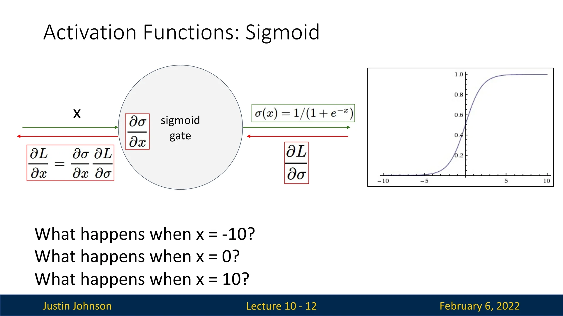
Figure 9.1: Sigmoid function visualization, highlighting gradient behavior at \( x = -10, 0, 10 \). Gradients are near zero at extreme values, causing vanishing gradients. Since \( \sigma (x) \) asymptotically approaches 0 for large negative values and 1 for large positive values, the derivative \( \sigma '(x) \) tends toward zero as well. This means that when activations reach extreme values, the network effectively stops learning due to near-zero gradients.
This effect compounds across layers in deep networks. Since gradient backpropagation involves multiplying local gradients, the product of many small values leads to an exponentially diminishing gradient, preventing effective weight updates in earlier layers.
- 2.
- Non Zero-Centered Outputs and Gradient Behavior: The sigmoid
function produces only positive outputs, \( \sigma (x) \in (0,1) \), leading to an imbalance in
weight updates. Consider the pre-activation computation at layer
\( \ell \):
\[ h_i^{(\ell )} = \sum _j w_{i,j}^{(\ell )} \sigma \left (h_j^{(\ell -1)}\right ) + b_i^{(\ell )} \]
where:
- \( h_i^{(\ell )} \) is the pre-activation output of the \( i \)-th neuron at layer \( \ell \).
- \( w^{(\ell )} \) and \( b^{(\ell )} \) are the weight matrix and bias vector at layer \( \ell \).
Since \( \sigma (x) \) is always positive, the gradient of the loss with respect to the weights at layer \( \ell \) follows:
\[ \frac {\partial L}{\partial w_{i,j}^{(\ell )}} = \frac {\partial L}{\partial h_i^{(\ell )}} \cdot \sigma \left (h_j^{(\ell -1)}\right ) \]
The key observation here is that all weight gradients \( \frac {\partial L}{\partial w_{i,j}^{(\ell )}} \) will have the same sign as the upstream gradient \( \frac {\partial L}{\partial h_i^{(\ell )}} \), because \( \sigma (h_j^{(\ell -1)}) \) is strictly positive. This introduces a significant issue:
- If the upstream gradient is positive, all weight updates will increase in the same direction.
- If the upstream gradient is negative, all weight updates will decrease in the same direction.
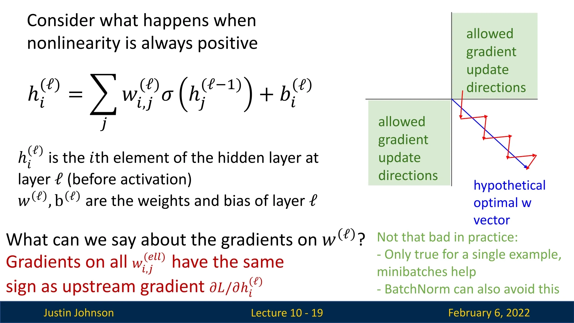
Figure 9.2: Gradient updates when using sigmoid activation: all gradients with respect to the weights have the same sign, leading to inefficient learning dynamics and potential oscillations. This behavior results in inefficient learning dynamics, where gradient descent updates are constrained in their movement, leading to oscillations and suboptimal convergence.
While using mini-batch gradient descent alleviates this issue somewhat—since different samples may introduce varying gradient directions, it remains an unnecessary limitation on the optimization process.
- 3.
- Computational Cost: The sigmoid function requires computing an
exponential function, which is computationally expensive, particularly on
CPUs. While when working with GPUs this increase of computation is
rather insignificant, as copying things onto the GPU to perform the
computation takes more time than this operation itself, the computational
overhead remains unnecessary compared to simpler alternatives
such as the ReLU function, which only requires a thresholding
operation.
Additionally, sigmoid’s computational inefficiency becomes more relevant when deploying models on edge devices or low-power hardware where efficiency is critical and GPU is not always at hand.
Among these issues, the vanishing gradient problem is the most critical, making sigmoid impractical for deep networks. The next section explores alternative activation functions that address these challenges.
The Tanh Activation Function
A closely related alternative to the sigmoid function is the hyperbolic tangent (\(\tanh \)) activation function, defined as:
\[ \tanh (x) = \frac {e^x - e^{-x}}{e^x + e^{-x}} \]
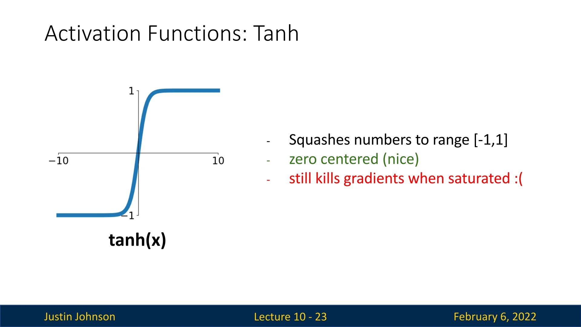
Unlike sigmoid, which outputs values in the range \((0,1)\), \(\tanh (x)\) squashes inputs to the range \((-1,1)\), making it zero-centered.
This addresses one of the issues of sigmoid—the fact that its outputs are strictly positive—allowing gradient updates to have both positive and negative directions, thereby reducing inefficient learning dynamics.
However, despite its advantage over sigmoid in terms of zero-centering, \(\tanh (x)\) still exhibits saturation effects. In the extreme positive or negative regions (\( x \gg 0 \) or \( x \ll 0 \)), \(\tanh (x)\) asymptotically approaches \(\pm 1\), causing its derivative to diminish:
\[ \tanh '(x) = 1 - \tanh ^2(x) \]
Since \(\tanh (x)\) approaches 1 or -1 in these regions, its derivative tends toward zero, leading to the vanishing gradient problem. This issue remains a major limitation for deep networks.
Due to this problem, \(\tanh (x)\) has also become an uncommon choice in modern deep learning architectures. The next sections introduces activation functions that better preserve gradients, enabling more stable training in deep networks.
9.2.2 Rectified Linear Units (ReLU) and Its Variants
The Rectified Linear Unit (ReLU) is a widely used activation function in modern deep learning due to its simplicity and effectiveness. It is defined as:
\[ f(x) = \max (0, x) \]
ReLU has several advantages over sigmoid and tanh:
- Computational Efficiency: It is the cheapest activation function, requiring only a sign check.
- Non-Saturating in Positive Regime: Unlike sigmoid and tanh, ReLU does not saturate for positive inputs, avoiding vanishing gradients when \( x > 0 \).
- Faster Convergence: Empirical results suggest that ReLU converges significantly faster than sigmoid or tanh (e.g., up to 6x faster in some cases).
However, ReLU is not without its drawbacks.
Issues with ReLU
Despite its advantages, ReLU has several notable weaknesses that can impact training stability and model performance:
- 1.
- Not Zero-Centered: Like sigmoid, ReLU outputs are strictly non-negative, leading to a gradient imbalance issue. Since negative inputs always map to zero, weight gradients for neurons processing only non-negative activations share the same sign, reducing the efficiency of gradient updates.
- 2.
- The ”Dead ReLU” Problem: If a neuron consistently receives
negative inputs, its activation is always zero, and its gradient remains
zero, effectively preventing any updates—this is known as a ”dead
ReLU.”
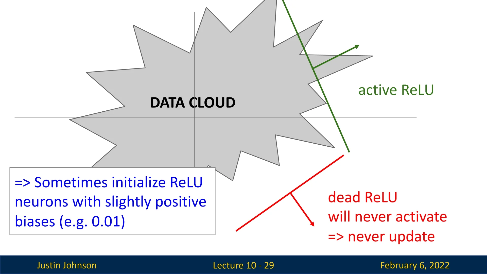
Figure 9.4: ReLU activation function and its failure cases. When inputs are negative, ReLU neurons become inactive, leading to dead ReLUs. This problem is particularly prevalent when using high learning rates or poor weight initialization. If all training samples produce negative pre-activations for a neuron, it remains inactive throughout training.
- 3.
- Exploding Activation Variance: In deeper networks, ReLU activations can cause an increase in activation variance due to their unbounded positive outputs. This can lead to instability during training, particularly when combined with high learning rates.
Mitigation Strategies for ReLU Issues
Several strategies exist to address these issues, some of which will be discussed in greater detail in later sections:
- Proper Weight Initialization: Using He initialization [216] ensures that ReLU neurons receive diverse activations at the start of training, reducing the likelihood of dead neurons.
- Lower Learning Rates with Batch Normalization: Applying batch normalization before or after the activation function helps control activation variance and stabilizes gradient updates, mitigating exploding activations.
- Alternative Activation Functions: Other activation functions such as Leaky ReLU, Parametric ReLU (PReLU), and Exponential Linear Unit (ELU) address some of ReLU’s limitations by modifying how negative inputs are handled. We will explore these alternatives in a later section.
While ReLU remains a popular activation function due to its simplicity and computational efficiency, understanding and addressing its limitations is crucial for designing stable and robust deep learning architectures.
Leaky ReLU and Parametric ReLU (PReLU)
A modification to ReLU, called Leaky ReLU, prevents neurons from completely dying by introducing a small negative slope for negative inputs:
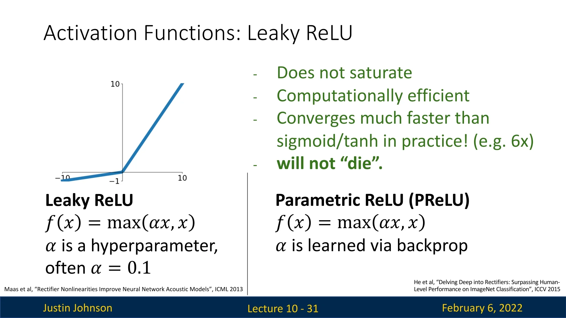
\(f(x) = \max (0.01x, x)\) This variant ensures that neurons never entirely deactivate, preserving gradient flow while maintaining computational efficiency. A further improvement, called Parametric ReLU (PReLU) [216], makes the negative slope \(\alpha \) a learnable parameter:
\[ f(x) = \max (\alpha x, x) \]
This means that during training, \(\alpha \) is updated alongside the other network parameters. It can be:
- A single shared \(\alpha \) across all layers.
- A unique \(\alpha \) per layer, learned independently.
While PReLU is an improvement over standard ReLU, it introduces a non-differentiable point at \( x = 0 \), making theoretical analysis more complex. However, in practice, this non-differentiability is rarely an issue.
Exponential Linear Unit (ELU)
Exponential Linear Units (ELU) [110] aim to address both the zero-centered output issue and dead ReLU problem. ELU is defined as:
\[ f(x) = \begin {cases} x, & x > 0 \\ \alpha (e^x - 1), & x \leq 0 \end {cases} \]
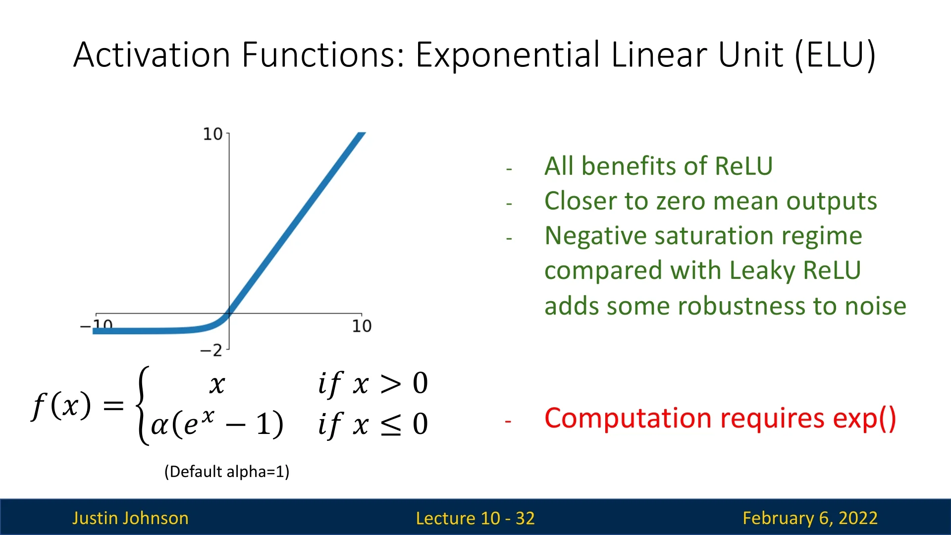
ELU has several advantages:
- Zero-Centered Outputs: Unlike ReLU, ELU allows negative activations, leading to a mean output closer to zero. This reduces the gradient imbalance issue present in ReLU, where all activations are strictly non-negative. Since the weight updates in gradient descent depend on the activation sign, having outputs symmetrically distributed around zero helps avoid directional bias in weight updates, leading to more stable and efficient learning.
- No Dead Neurons: The negative exponential ensures that neurons always receive a nonzero gradient, preventing dead neurons (a problem in ReLU where negative inputs always map to zero, leading to zero gradients). With ELU, even if a neuron’s input is negative, it will still produce a small nonzero gradient due to the exponential term, allowing learning to continue.
- Robustness to Noise: The negative saturation regime in ELU makes it more resistant to small input perturbations compared to ReLU. This is because for highly negative inputs, the ELU function approaches a stable asymptotic value instead of continuing to decrease indefinitely. As a result, small variations in input values within the negative region cause only minimal changes in activation, reducing sensitivity to minor input noise and improving generalization.
The main drawback of ELU is its computational cost, as it requires computing \( e^x \) for negative values, making it more expensive than ReLU on some hardware.
Scaled Exponential Linear Unit (SELU)
Building on the Exponential Linear Unit (ELU), the Scaled Exponential Linear Unit (SELU) [310] was designed to produce self-normalizing neural networks—models whose activations naturally converge toward zero mean and unit variance as signals propagate through layers. This self-stabilizing behavior helps prevent the vanishing or exploding activations that commonly arise when layer outputs drift in scale through deep compositions.
SELU introduces two fixed constants, \(\alpha \approx 1.6733\) and \(\lambda \approx 1.0507\), in its formulation: \[ \mbox{SELU}(x) = \lambda \begin {cases} x, & x > 0 \\ \alpha (e^x - 1), & x \leq 0 \end {cases}. \] The positive branch (\(\lambda x\)) slightly amplifies activations to preserve variance, while the negative branch (\(\lambda \alpha (e^x - 1)\)) pushes the mean back toward zero. Together, they form a feedback mechanism that keeps the activation distribution close to equilibrium—acting like an internal “thermostat” for layer statistics and sustaining healthy gradient flow by keeping neurons within their responsive range.
Self-Normalization Principle The self-normalizing property arises from a fixed-point analysis of how the mean and variance evolve through layers. Assuming approximately independent, zero-mean, unit-variance Gaussian inputs, SELU was derived so that its expected output statistics satisfy \[ \mathbb {E}[y] = 0, \quad \mathrm {Var}(y) = 1, \] and small deviations from these values contract back toward equilibrium over depth. The constants \(\alpha \) and \(\lambda \) were solved analytically to satisfy these fixed-point equations and verified via the Banach fixed-point theorem, ensuring that even very deep feedforward networks maintain stable activation and gradient magnitudes without explicit normalization layers such as Batch Normalization. Empirically, this allows training hundreds of fully connected layers with minimal degradation.
Requirements and Practical Use For SELU to exhibit true self-normalization, several conditions must hold:
- Initialization: Weights should follow LeCun normal initialization, \(\mathcal {N}(0, 1/n_{\mbox{in}})\), matching the fixed-point variance assumption.
- Architecture: The theory assumes fully connected, feedforward layers with approximately independent activations. Correlated or skip-connected structures (e.g., CNNs, RNNs, or ResNets) may violate these assumptions and weaken the effect.
- Regularization: Standard dropout disrupts mean and variance; AlphaDropout must be used instead, which maintains SELU-compatible activation statistics.
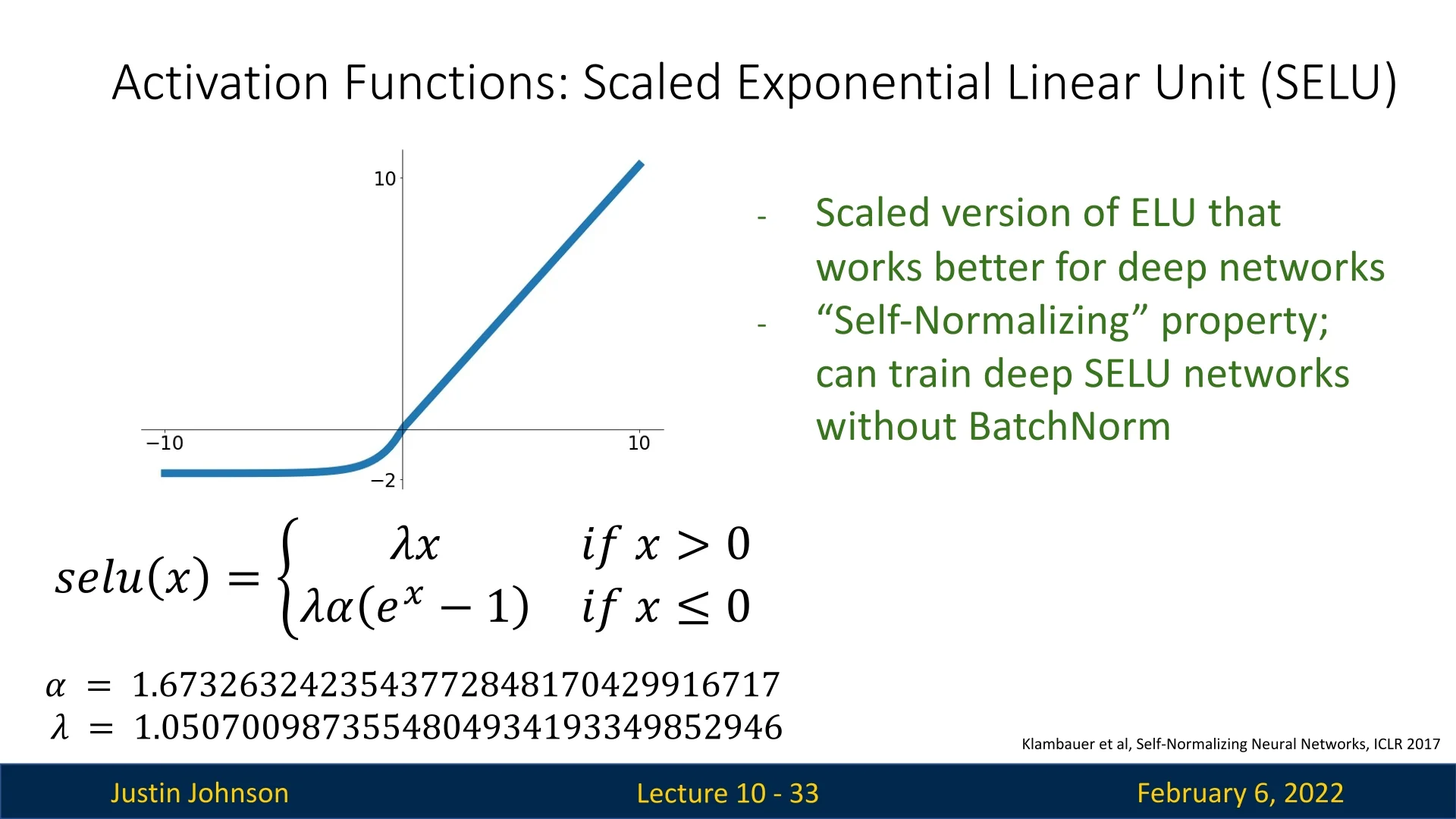
Advantages and Limitations SELU offers an elegant theoretical route to stable activations and consistent gradient flow without normalization layers. However, its guarantees depend on strict conditions, and its exponential term adds modest computational cost. In modern architectures, ReLU or GELU combined with Batch Normalization provides comparable stability with fewer constraints. Nonetheless, for deep fully connected networks trained under proper initialization and regularization, SELU remains a theoretically grounded and practically effective choice.
Gaussian Error Linear Unit (GELU)
The Gaussian Error Linear Unit (GELU) is an activation function introduced by Hendrycks and Gimpel [224], designed to provide smoother, more data-dependent activation compared to ReLU. Unlike standard piecewise linear activations, GELU applies a probabilistic approach, allowing smoother transitions and improved gradient flow.
Definition The GELU activation function is defined as:
\[ \mbox{GELU}(x) = x P(X \leq x) = x \cdot \frac {1}{2} \left (1 + \mbox{erf} \left ( \frac {x}{\sqrt {2}} \right ) \right ), \]
where \(\mbox{erf}(\cdot )\) is the Gaussian error function.
This formulation can be interpreted as applying element-wise stochastic regularization, where smaller values of \( x \) are more likely to be suppressed, while larger values pass through more freely.
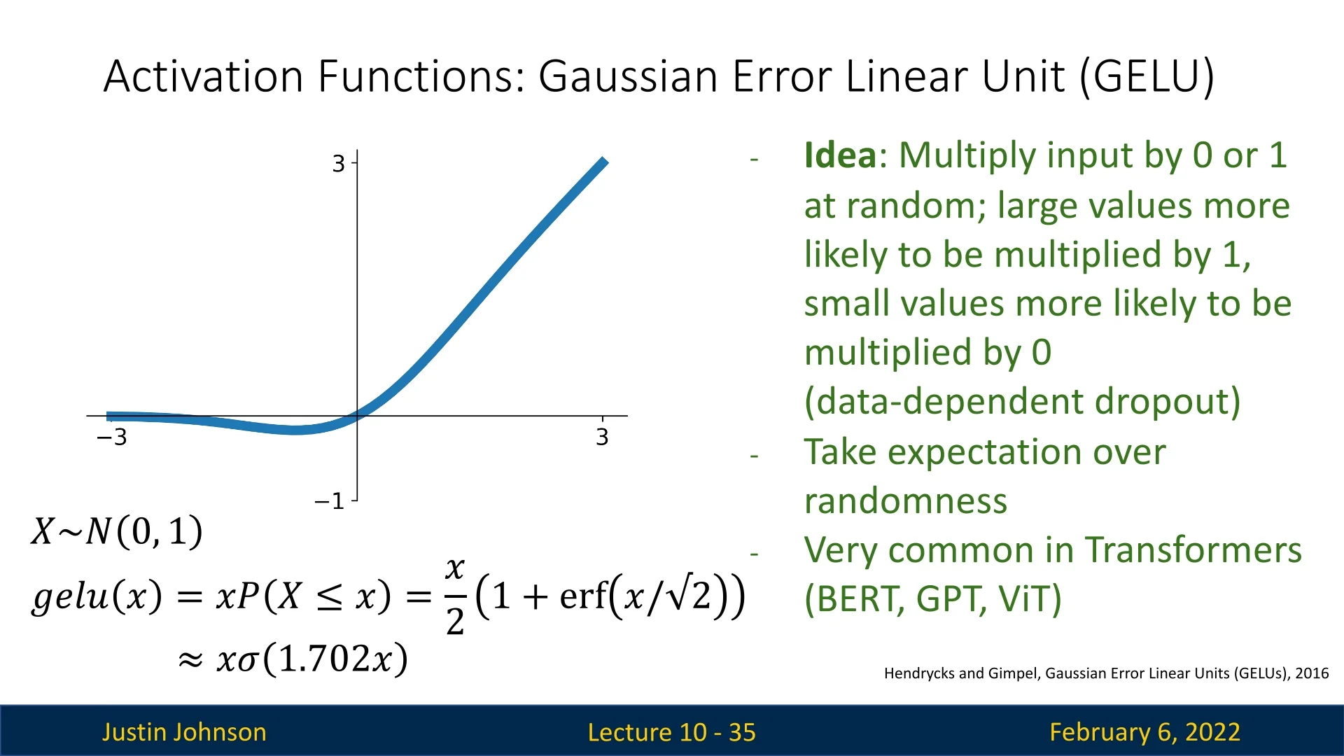
For computational efficiency, GELU is often approximated as:
\[ \mbox{GELU}(x) \approx 0.5 x \left ( 1 + \tanh \left ( \sqrt {\frac {2}{\pi }} \left (x + 0.044715 x^3 \right ) \right ) \right ). \]
This approximation is commonly used in deep learning frameworks to avoid directly computing the error function, which can be expensive.
- Smooth Activation Improves Gradient Flow Rather than a hard cutoff at zero, GELU gradually suppresses negative inputs. This softer transition helps maintain stable gradients throughout training, mitigating “dead neurons” seen in ReLUs.
- Adaptive, Data-Dependent Sparsity GELU provides a continuous relaxation of dropout: smaller inputs are more likely to be dampened, while larger inputs pass largely intact. This implicit stochasticity can enhance regularization and robustness, especially in noisy data regimes.
- Richer Expressiveness Both ELU and GELU allow negative inputs to contribute to the output, but they do so in different ways. ELU applies a fixed exponential decay to negative values, causing them to saturate toward a constant (typically \(-\alpha \)) for very low inputs. In contrast, GELU multiplies the input by a smooth probability factor, \( \Phi (x) \), derived from the Gaussian cumulative distribution. This means that GELU scales negative inputs in a continuous and data-dependent manner rather than compressing them to a fixed value. As a result, GELU can preserve subtle variations in the negative range, offering a more nuanced transformation that improves the network’s ability to model complex patterns.
- Empirical Performance Gains Studies report that models employing GELU frequently converge faster and generalize better, notably in NLP tasks (BERT, GPT) and vision tasks (ViT). This benefit is attributed to GELU’s smoother gradient flow and retention of meaningful negative signals.
- ReLU: Although ReLU is computationally simpler, it “zeroes out” negative inputs entirely, risking dead neurons and abrupt gradient cutoffs. In contrast, GELU keeps certain negative inputs partially active, fostering more informative gradients.
- ELU: ELU reduces saturation for negative values by an exponential term, but still imposes a fixed shape for negative activations. GELU instead adjusts activation magnitudes continuously based on their magnitude, preserving a more natural, data-driven activation profile.
Computational Considerations The primary drawback of GELU is its computational cost. The use of the \(\mbox{erf}(\cdot )\) function introduces additional complexity compared to simpler activations like ReLU. However, its empirical success in large-scale models, particularly in NLP and vision tasks, often justifies the added computational overhead.
In summary, GELU is a powerful activation function that enhances model expressiveness and stability, particularly in architectures relying on self-attention mechanisms. Its widespread adoption in modern deep learning models, including Transformers, highlights its practical advantages over traditional activation functions.
Enrichment 9.2.3: Swish: A Self-Gated Activation Function
Swish, introduced by [520], is a smooth, non-monotonic activation function defined as:
\[ f(x) = x \cdot \sigma (\beta x) = x \cdot \frac {1}{1 + e^{-\beta x}} \]
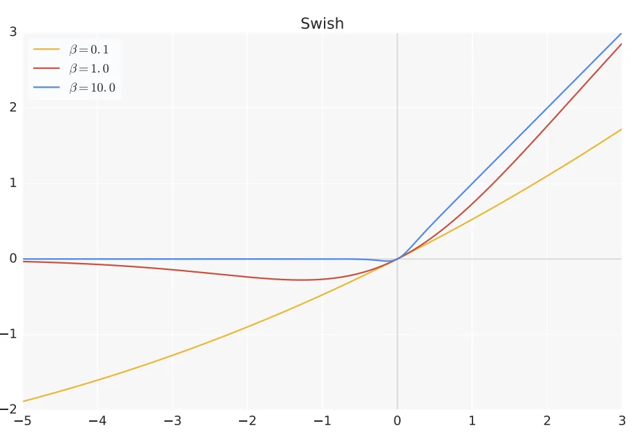
where \(\sigma (\beta x)\) is the standard sigmoid function, and \(\beta \) is a parameter that controls the shape of the activation. In the simplest case, \(\beta = 1\), resulting in:
\[ f(x) = x \cdot \sigma (x) = \frac {x}{1 + e^{-x}} \]
Unlike ReLU, Swish is self-gated, meaning the activation dynamically scales itself based on its input. This property leads to several advantages in deep learning.
Advantages of Swish
Swish exhibits a combination of desirable properties that make it a strong alternative to ReLU-based activations:
-
Smooth Activation: Unlike ReLU, Swish is continuously differentiable, which helps maintain stable gradient flow and improves optimization dynamics.
- Non-Monotonicity: Swish does not strictly increase or decrease across its domain. This allows it to capture more complex relationships in the data compared to monotonic functions like ReLU, potentially enhancing feature learning.
- No Dead Neurons: Unlike ReLU, which can lead to permanently inactive neurons (when weights drive activations below zero), Swish ensures that even negative values contribute to learning, as \(\sigma (x)\) never completely zeroes them out.
- Improved Expressiveness: The self-gating property allows the function to act as a smooth interpolation between linear and non-linear behavior, adapting dynamically across different network layers.
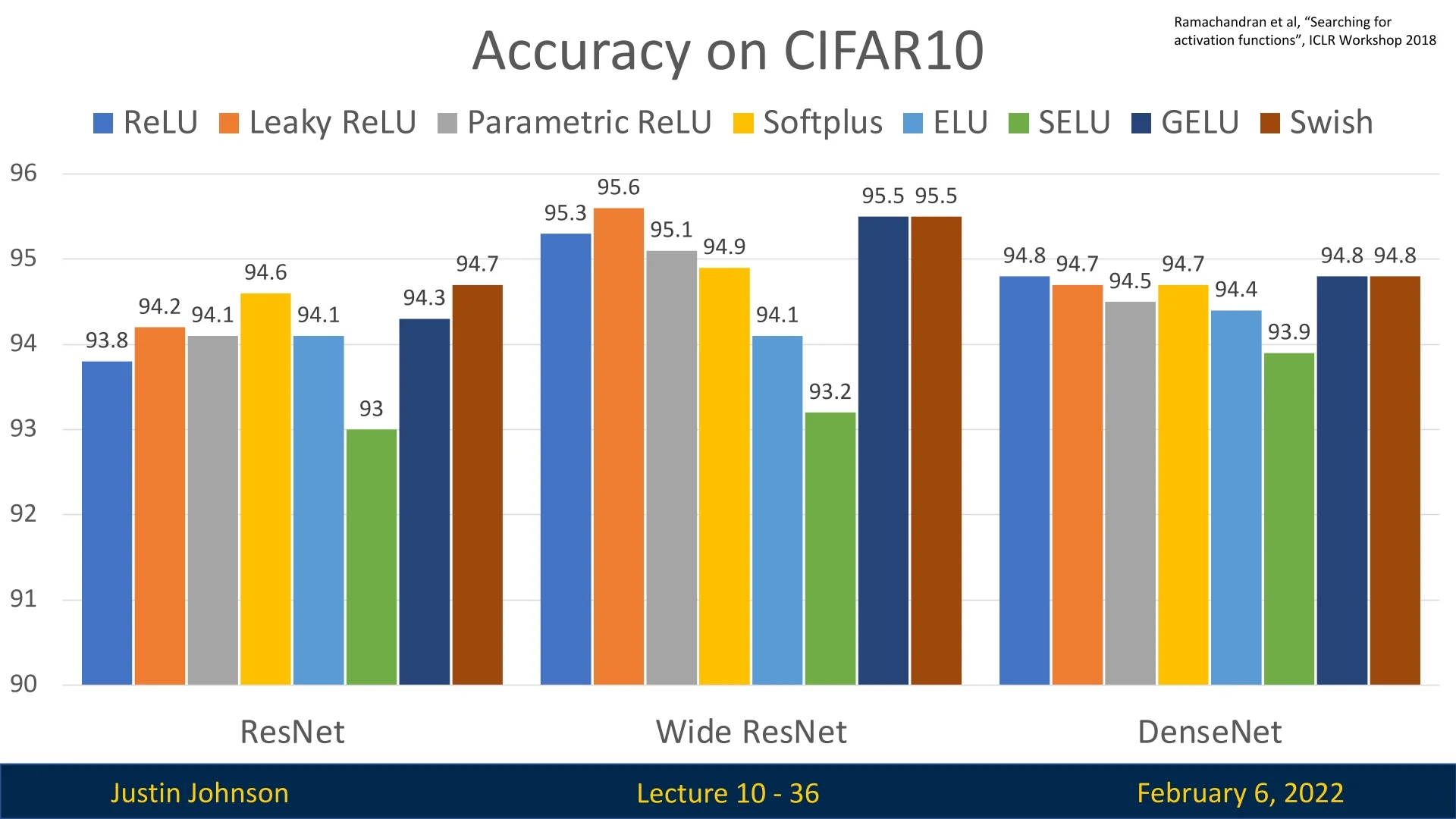
- State-of-the-Art Performance: Swish has been empirically shown to outperform ReLU in large-scale models like EfficientNet, where careful architecture optimization is crucial [621].
Disadvantages of Swish
Despite its strengths, Swish has some drawbacks:
- Higher Computational Cost: The sigmoid function \(\sigma (x)\) requires computing an exponential, making Swish computationally more expensive than ReLU. This can be a limiting factor in resource-constrained environments like mobile or edge devices.
- Lack of Widespread Adoption: Although Swish has shown improvements in performance, ReLU remains dominant due to its simplicity and efficiency, particularly in standard architectures.
- Sensitivity to \(\beta \): While \(\beta \) can be a learnable parameter, tuning it effectively across different architectures is not always straightforward.
Comparison to Other Top-Tier Activations
Swish competes with other top-tier activation functions like GELU, ELU, and SELU. The following comparisons highlight where Swish stands:
- Swish vs. GELU: Both are smooth and non-monotonic, making them superior to ReLU in terms of expressiveness. GELU is particularly useful in Transformer models, while Swish has been optimized for CNNs. Swish has a learnable component (\(\beta \)), whereas GELU is entirely data-driven.
- Swish vs. ELU: ELU is zero-centered and smooth, making it more stable than ReLU. However, it enforces a sharp exponential decay in the negative regime, while Swish allows a more gradual transition. Swish generally performs better in deep networks, especially when \(\beta \) is optimized.
- Swish vs. SELU: SELU is explicitly designed for self-normalization and aims to remove the need for BatchNorm. While SELU works well in fully connected architectures, Swish is more versatile and better suited for CNNs and Transformers.
- Swish vs. ReLU: ReLU remains the fastest and most commonly used activation function. Swish generally outperforms ReLU in deeper architectures, but the computational cost of the sigmoid component makes ReLU preferable in most applications.
Conclusion
Swish is a promising activation function that builds upon ReLU’s strengths while mitigating some of its weaknesses. It has been particularly effective in CNNs such as EfficientNet and remains a viable alternative for deep learning models. However, due to its increased computational cost and lack of widespread adoption, ReLU continues to dominate in many architectures. Nevertheless, as neural networks become deeper and more complex, Swish presents a compelling option for researchers seeking improved optimization and expressiveness.
9.2.3 Choosing the Right Activation Function
The choice of activation function plays a crucial role in deep learning, impacting gradient flow, convergence speed, and final performance. However, in most cases, ReLU is sufficient and a reliable default choice.
General Guidelines for Choosing an Activation Function
Based on empirical findings, the following recommendations can guide activation function selection:
- ReLU is usually the best default choice: It is computationally efficient, simple to implement, and provides strong performance across various architectures.
- Consider Leaky ReLU, ELU, SELU, GELU or Swish when seeking marginal gains: These activations can help squeeze out small improvements, particularly in deeper networks.
- Avoid Sigmoid and Tanh: These functions cause vanishing gradients, leading to poor optimization dynamics and slower convergence.
- Some recent architectures use GELU instead of ReLU, but the gains are minimal: GELU is commonly found in Transformer-based models like BERT and GPT, but its improvements over ReLU are typically small.
9.3 Data Pre-Processing
Before feeding data into a neural network, it is crucial to perform pre-processing to make it more suitable for efficient training. Proper pre-processing ensures that input features are well-behaved, leading to improved optimization stability and faster convergence.
9.3.1 Why Pre-Processing Matters
Neural networks operate in high-dimensional spaces, and poorly scaled inputs can significantly hinder learning. The key goals of pre-processing are:
- Centering the Data: Bringing the data closer to the origin by subtracting the mean.
- Rescaling Features: Ensuring that all features have similar variance to prevent dominant features from overpowering others during training.
Without pre-processing, different input features may exist at vastly different scales, making optimization challenging. By ensuring that inputs have a mean of zero and similar variances, gradient updates become more consistent across all features.
9.3.2 Avoiding Poor Training Dynamics
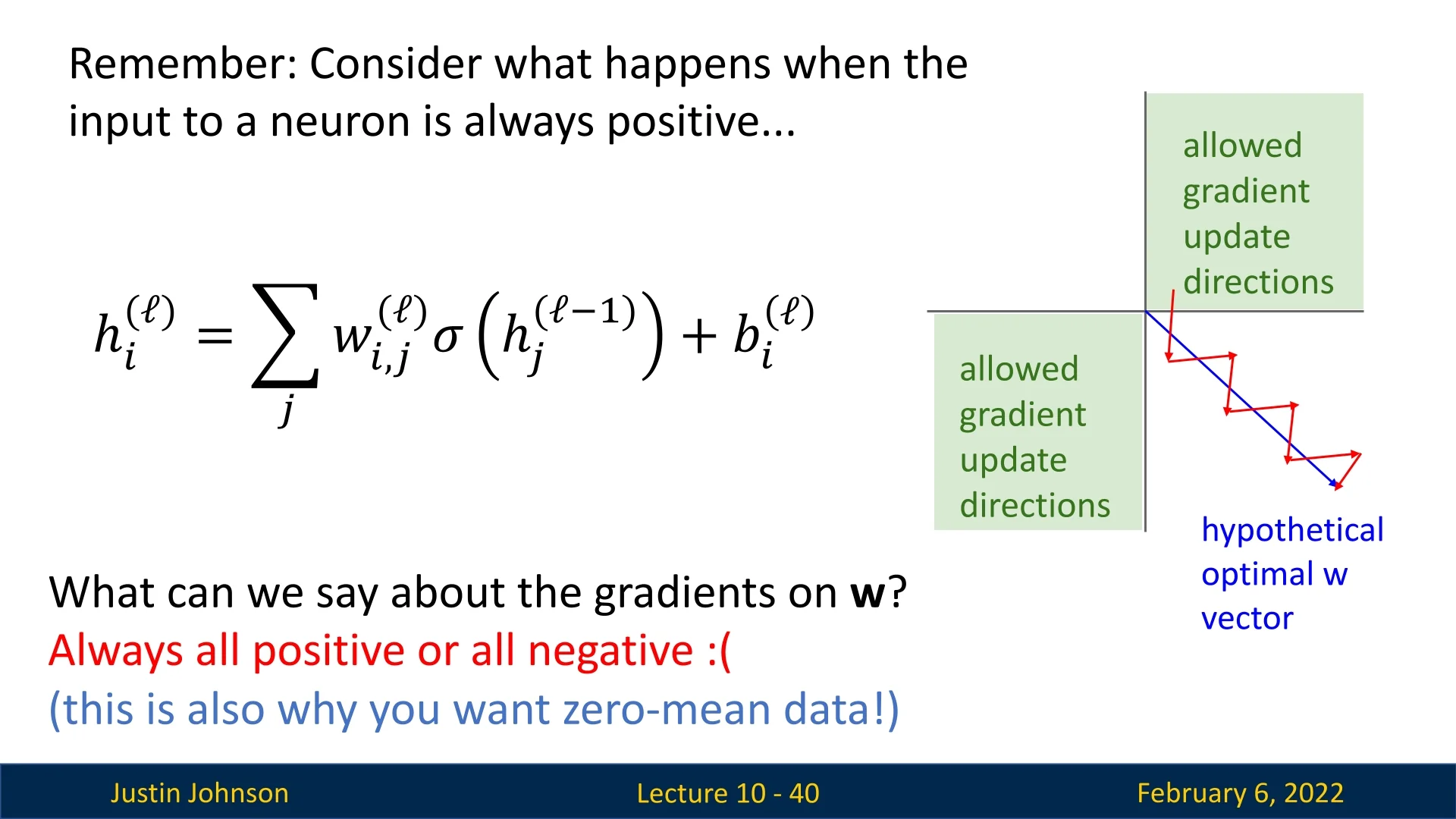
Pre-processing mitigates unstable or inefficient training by keeping neuron inputs well-centered and scaled. When inputs are biased to one side of zero or have widely varying magnitudes, activation functions respond unevenly—causing gradients to become correlated or vanish. For instance, if all inputs to a ReLU layer are positive, every neuron operates in its linear regime, and all weight gradients share the same sign. This restricts the optimizer to move in a single direction, producing inefficient zig-zag dynamics where updates oscillate rather than progress directly toward the optimum.
Centering inputs around zero introduces both positive and negative activations, allowing gradients to vary in sign and direction. Scaling to unit variance keeps pre-activations within the responsive range of nonlinearities (e.g., avoiding saturation in sigmoid or tanh), ensuring gradients remain balanced and optimization proceeds smoothly.
9.3.3 Common Pre-Processing Techniques
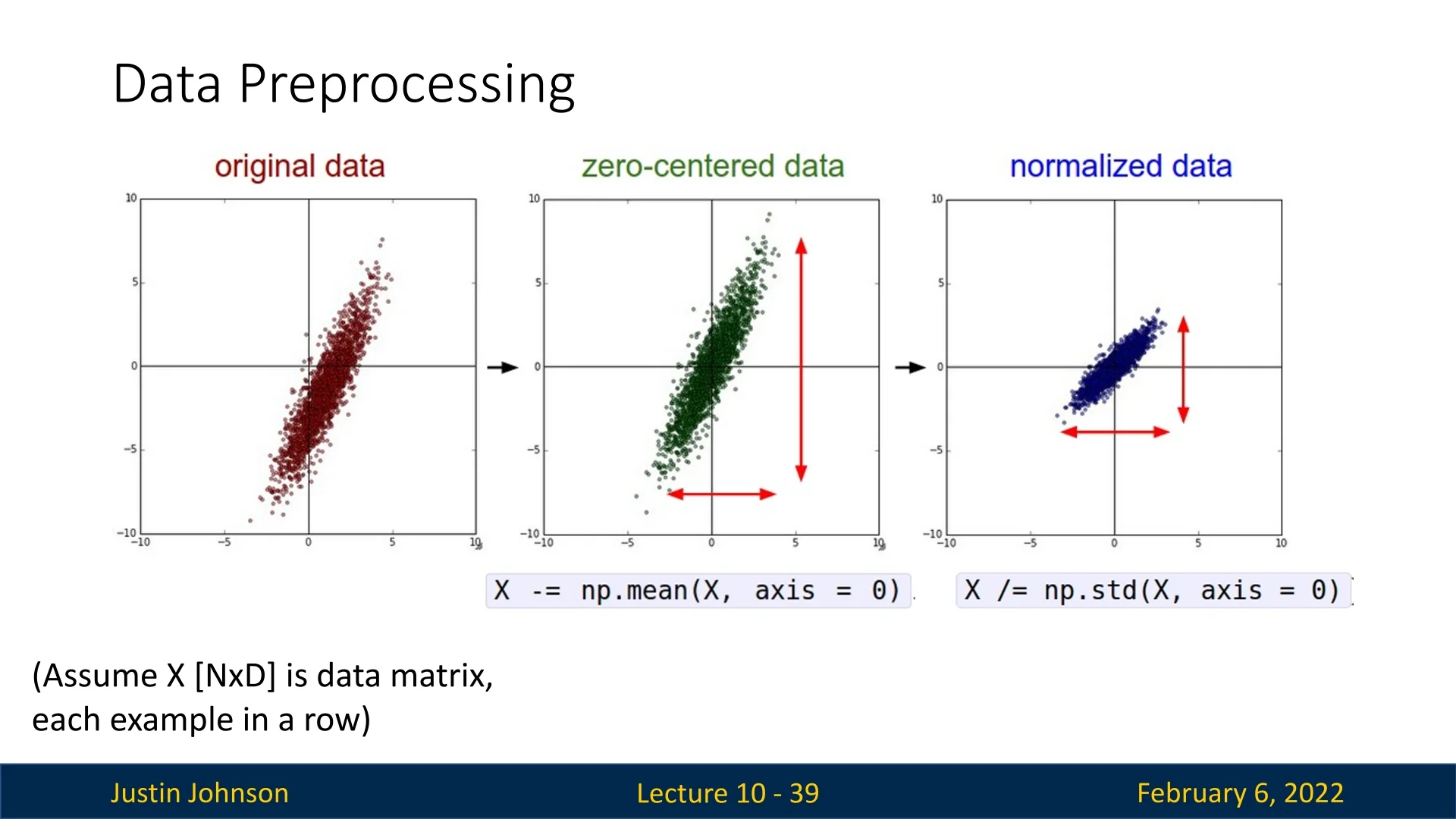
For images, a widely used technique is Mean Subtraction and Standardization: Compute the mean and standard deviation of pixel values across the training dataset, subtract the mean, and divide by the standard deviation.
Less ideal but still very common pre-processing technique for images is simply dividing each pixel value by 255 to keep them in the range \([0,1]\).Other data types, such as low-dimensional vectors, may require more sophisticated transformations beyond simple mean subtraction and scaling. Two common techniques are:
- Decorrelation: This process transforms the data so that its covariance matrix becomes diagonal, meaning that the features become uncorrelated with each other. Many machine learning algorithms, particularly those relying on linear operations, work more efficiently when the input features are independent. Removing correlations between features can make optimization more stable and improve convergence rates.
- Whitening: A further step beyond decorrelation, whitening transforms the data such that its covariance matrix becomes the identity matrix. This means that not only are features uncorrelated, but they also have unit variance. Whitening ensures that all features contribute equally to learning, preventing some from dominating due to larger magnitudes. A common way to achieve whitening is through ZCA (Zero-phase Component Analysis), a variant of PCA that applies an orthogonal transformation to maintain the structure of the original data while normalizing its covariance.
Why are these techniques less common for images? While decorrelation and whitening can be beneficial in feature-based learning systems, they are rarely used in deep learning for image data. This is because convolutional neural networks (CNNs) inherently learn hierarchical feature representations, making the manual decorrelation of input features less necessary. Additionally, images exhibit strong local correlations (e.g., neighboring pixels tend to have similar intensities), which CNNs are designed to exploit rather than eliminate. Whitening could disrupt these spatial patterns, potentially harming the model’s ability to recognize meaningful structures.
However, for structured datasets, tabular data, or domains like speech recognition, where input features may exhibit high redundancy, applying decorrelation and whitening can significantly improve model performance.
A fundamental tool in this domain is Principal Component Analysis (PCA), which helps in both pre-processing and visualization of high-dimensional embeddings. PCA identifies the principal axes of variation in the data, allowing us to decorrelate features and, if desired, apply whitening. A good introduction to PCA can be found in this video by Steve Brunton.
9.3.4 Normalization for Robust Optimization
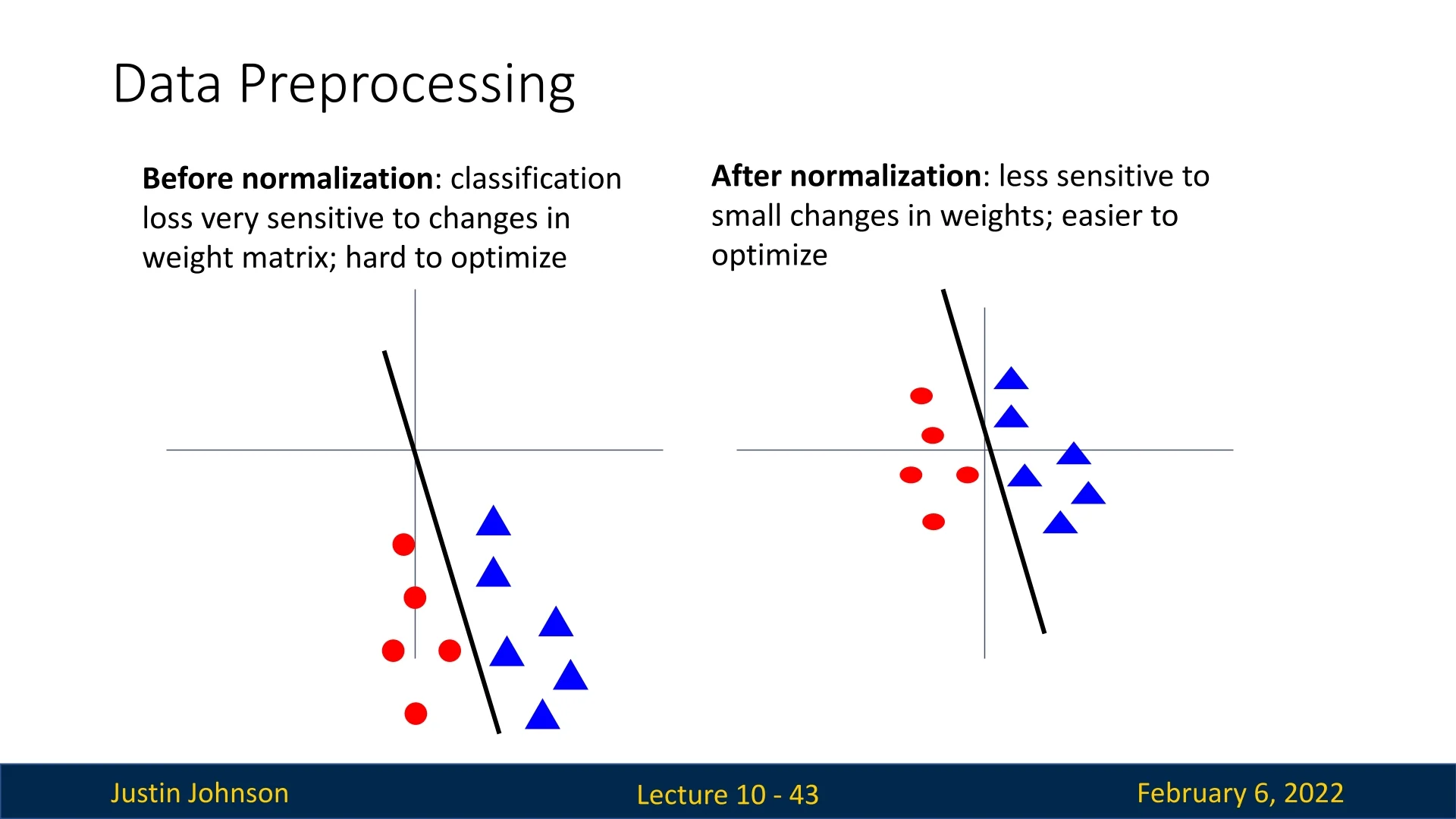
Another intuitive way to understand the benefits of normalization is by examining how it impacts the learning process. When input data is unnormalized:
- The classification loss becomes highly sensitive to small changes in weight values.
- Optimization becomes difficult due to erratic updates.
Conversely, after normalization:
- Small changes in weight values produce more predictable adjustments.
- The learning process becomes more stable and easier to optimize.
9.3.5 Maintaining Consistency During Inference
A critical point in pre-processing is ensuring that the same transformations applied during training must be applied during inference. If the test data is not normalized in the same way as the training data, the network will fail to generalize correctly.
9.3.6 Pre-Processing in Well-Known Architectures
Different deep learning architectures employ various pre-processing techniques:
- AlexNet: Subtracts the mean image computed across the dataset.
- VGG: Normalizes each color channel separately by subtracting the mean RGB value.
- ResNet: Normalizes pixel values using dataset-wide mean and standard deviation.
9.4 Weight Initialization
Choosing an appropriate weight initialization strategy is crucial for training deep neural networks effectively. Poor weight initialization can lead to problems such as vanishing gradients, exploding gradients, and symmetry issues, ultimately hindering optimization. In this section, we explore different initialization techniques, highlighting their advantages and limitations.
9.4.1 Constant Initialization
A naive approach to weight initialization is to assign all weights the same constant value, such as zero or one. While this may appear harmless, it fundamentally breaks the diversity required for effective learning. Regardless of the chosen constant, this strategy leads to the symmetry problem: all neurons in a layer compute identical outputs, receive identical gradients, and therefore evolve identically. The network fails to learn diverse features, effectively collapsing each layer to a single neuron.
There are two primary cases to consider: zero initialization and nonzero constant initialization.
Zero Initialization
Initializing all weights and biases to zero represents the most extreme form of the symmetry problem. When every neuron in a layer begins with identical parameters, they compute the same outputs, receive identical gradients, and update in exactly the same way—preventing any neuron from learning a distinct feature. In effect, the entire layer collapses into a single neuron.
Forward Pass If all weights and biases in a layer are initialized to zero, then for every neuron \( i \): \[ z_l^{(i)} = \sum _j a_{l-1}^{(j)} \cdot 0 + 0 = 0, \qquad a_l^{(i)} = g(0). \] This means all neurons produce the same activation value, regardless of input. For activations where \( g(0) = 0 \), such as ReLU and \(\tanh \), every neuron outputs zero. For sigmoid, \( g(0) = 0.5 \), yielding a constant activation across the entire layer.
Backward Pass and Gradient Collapse The weight gradient for a given neuron is \[ \frac {\partial \mathcal {L}}{\partial W_l^{(i,j)}} = \frac {\partial \mathcal {L}}{\partial a_l^{(i)}} \cdot g'(z_l^{(i)}) \cdot a_{l-1}^{(j)}. \] Since all \( z_l^{(i)} \) and \( a_l^{(i)} \) are identical, the local derivative \( g'(z_l^{(i)}) \) and the upstream gradient \( \frac {\partial \mathcal {L}}{\partial a_l^{(i)}} \) are also identical across neurons. Consequently, all weights receive the same update: \[ \Delta W_l^{(i,j)} \propto g'(0) \cdot a_{l-1}^{(j)}. \] For ReLU, \( g'(0) = 0 \), so all weight updates vanish completely: \[ \frac {\partial \mathcal {L}}{\partial W_l} = 0. \] The network cannot learn at all. Even for sigmoid, where \( g'(0) = 0.25 \), the gradients are nonzero but identical across neurons, so symmetry persists—each neuron evolves identically and no specialization occurs.
Intuitive View Zero initialization is like asking every neuron to start with the same opinion and learn from identical feedback: none will ever disagree or diverge. Without differences in their initial parameters, all neurons in a layer respond the same way to every input and gradient, leaving the network incapable of learning complex, varied representations.
Conclusion Zero initialization causes both symmetry and gradient collapse:
- Neurons produce identical activations (\(a_l^{(i)} = a_l^{(k)}\) for all \(i,k\)).
- Gradients vanish for ReLU/tanh or remain uniform for sigmoid.
- The network fails to break symmetry, effectively reducing each layer to a single unit.
Nonzero Constant Initialization
Even when all weights are initialized to a nonzero constant value, such as \( c = 1 \), the symmetry problem remains—though gradients no longer vanish, neurons still evolve identically.
Forward Pass For any constant \( c \) and bias \( d \): \[ W_l^{(i,j)} = c, \quad b_l^{(i)} = d. \] Then each neuron’s pre-activation is identical: \[ z_l^{(i)} = \sum _j a_{l-1}^{(j)} c + d, \] yielding the same activation \( a_l^{(i)} = g(z_l) \) for all \( i \). Thus, every neuron processes inputs in the same way, eliminating feature diversity.
Backward Pass During backpropagation, \[ \frac {\partial \mathcal {L}}{\partial W_l^{(i,j)}} = \frac {\partial \mathcal {L}}{\partial a_l^{(i)}} \cdot g'(z_l^{(i)}) \cdot a_{l-1}^{(j)}. \] Since \( a_l^{(i)} \) and \( g'(z_l^{(i)}) \) are identical across neurons, all gradients are equal. The update step applies uniformly to all weights: \[ W_l^{(i,j)} \leftarrow W_l^{(i,j)} - \alpha \cdot \mbox{constant} \cdot a_{l-1}^{(j)}. \] The weights remain identical over time, and the layer continues to behave as a single neuron.
Summary Whether initialized to zero or any other constant, all neurons in a layer start in perfect symmetry. Since they receive identical gradients, they remain symmetric, preventing meaningful learning.
To avoid this collapse, symmetry must be broken through random initialization, where small differences in initial weights allow neurons to learn distinct features. Randomized schemes such as Xavier and He initialization achieve this by preserving activation variance while ensuring statistical diversity—a topic explored next.
9.4.2 Breaking Symmetry: Random Initialization
To prevent the symmetry problem, weights must be initialized with randomness. A simple approach is to sample them from a uniform or normal distribution:
\[ w_{i,j} \sim U\left (-\frac {1}{\sqrt {n}}, \frac {1}{\sqrt {n}}\right ) \quad \mbox{or} \quad w_{i,j} \sim N(0, \sigma ^2), \]
where \( n \) is the number of inputs to the neuron (in case of FC networks, the number of neurons in the previous layer). This ensures slight variations between neurons, allowing them to learn different features.
However, naive random initialization is not sufficient. Without controlling variance, deep networks may suffer from:
- Vanishing Gradients: Small weights lead to progressively smaller activations, causing gradients to shrink during backpropagation.
- Exploding Gradients: Large weights amplify activations, leading to unstable updates and divergence.
- Inefficient Optimization: Poor initialization can make optimization highly sensitive to learning rate selection.
These issues arise because errors accumulate across layers, affecting gradient flow and optimization stability.
9.4.3 Variance-Based Initialization: Ensuring Stable Information Flow
In deep networks, information must flow through many layers during both the forward and backward passes. If the magnitude of activations or gradients changes dramatically across layers, learning becomes unstable: some layers dominate while others effectively stop learning. Variance-based initialization aims to prevent this by designing weight distributions that keep the scale of signals statistically consistent throughout the network.
Key Requirements for Stable Propagation For stable learning, we want the variance of both forward activations and backward gradients to remain roughly constant across layers: \[ \forall l, \quad \operatorname {Var}[z^l] \approx \operatorname {Var}[z^{l+1}], \qquad \forall l, \quad \operatorname {Var}\!\left [\frac {\partial \mathcal {L}}{\partial W^l}\right ] \approx \operatorname {Var}\!\left [\frac {\partial \mathcal {L}}{\partial W^{l+1}}\right ]. \] Here:
- \( z^l = W^l a^{l-1} + b^l \) denotes the pre-activation at layer \( l \), before applying the nonlinearity.
- \( a^{l-1} = g(z^{l-1}) \) is the previous layer’s activation output.
- \( \frac {\partial \mathcal {L}}{\partial W^l} \) represents the gradient of the loss with respect to the weights at layer \( l \).
These two stability conditions correspond to the two directions of signal flow in a network:
- Forward variance preservation ensures that activations maintain a consistent scale across layers, preventing values from exploding or vanishing as they move deeper into the network.
- Backward variance preservation ensures that gradients maintain a consistent magnitude as they propagate backward during training, allowing each layer to receive meaningful updates.
Intuitively, forward propagation is about how information travels through the model’s neurons, while backward propagation is about how learning signals travel back through its weights. If either direction suffers distortion—amplification or attenuation—training can collapse.
Why This Matters When these variances are not balanced, deep networks exhibit one of two well-known failure modes:
- Exploding Gradients: If activations grow across layers (\( \operatorname {Var}[z^l] \gg 1 \)), backpropagated gradients accumulate multiplicatively, producing massive updates and numerical instability (e.g., NaN weights).
- Vanishing Gradients: If activations shrink (\( \operatorname {Var}[z^l] \ll 1 \)), gradients decay exponentially as they move backward, starving early layers of useful learning signals.
These problems compound with depth: even small imbalances in variance per layer can produce exponential growth or decay across dozens of layers. Hence, proper initialization acts like a “pressure regulator,” keeping signal magnitudes stable so that gradients remain in a trainable range.
Understanding the Forward Requirement Forward stability determines how information propagates through depth. Each neuron aggregates its inputs via the weights and transforms them through a nonlinearity. For neuron \( i \) in layer \( l \): \[ z_l^{(i)} = \sum _j W_l^{(i,j)} a_{l-1}^{(j)} + b_l^{(i)}. \] Assuming independent, zero-mean activations \( a_{l-1}^{(j)} \) with variance \( \sigma _a^2 \) and weights \( W_l^{(i,j)} \) drawn with zero mean and variance \( \sigma _w^2 \), the pre-activation variance becomes: \[ \operatorname {Var}[z_l^{(i)}] = n_{\mbox{in}} \cdot \sigma _w^2 \cdot \sigma _a^2, \] where \( n_{\mbox{in}} \) (the fan-in) is the number of inputs per neuron.
If \( \sigma _w^2 \) is too large, \( \operatorname {Var}[z_l] \) grows exponentially with depth—causing exploding activations: neurons saturate (sigmoid/tanh) or output excessively large values (ReLU), both of which degrade gradients and destabilize training. If \( \sigma _w^2 \) is too small, \( \operatorname {Var}[z_l] \) decays exponentially—causing vanishing activations: layer outputs collapse toward zero, losing representational diversity and producing near-zero gradients. Thus, controlling forward variance is essential not just for numerical stability but to keep activations within their informative regime, where \( g'(z) \) remains nonzero and gradients can flow.
Understanding the Backward Requirement Backward stability governs how error signals propagate during gradient descent. Each weight gradient depends on both the upstream error and the local activation: \[ \frac {\partial \mathcal {L}}{\partial W_l^{(i,j)}} = \frac {\partial \mathcal {L}}{\partial z_l^{(i)}} \cdot a_{l-1}^{(j)}. \] Consequently, the variance of weight gradients satisfies: \[ \operatorname {Var}\!\left [\frac {\partial \mathcal {L}}{\partial W_l}\right ] \propto \operatorname {Var}\!\left [\frac {\partial \mathcal {L}}{\partial z_l}\right ] \cdot \operatorname {Var}[a_{l-1}]. \] If the forward pass amplifies activations, gradients magnify as well—eventually exploding. If activations diminish, gradients vanish, leaving early layers effectively frozen. Hence, the forward and backward requirements are inseparable: stable gradient flow depends on maintaining balanced activation variance, and vice versa.
Variance-preserving initialization methods, such as Xavier and Kaiming, are explicitly derived to satisfy both conditions simultaneously—choosing \( \sigma _w^2 \) so that neither activations nor gradients drift in scale as signals traverse the network.
Challenges in Practice Achieving both forward and backward stability simultaneously is difficult because nonlinear activation functions distort the signal. For example:
- Nonlinearities like ReLU or tanh change the distribution of activations and their variance.
- The number of input and output connections (fan-in and fan-out) differs across layers.
- Small deviations accumulate multiplicatively in deep networks, amplifying drift.
As a result, ideal variance preservation can only be approximated through careful scaling of the initial weight distribution.
Toward Practical Solutions Variance-based initialization provides the foundation for all modern initialization schemes. The upcoming methods—Xavier (Glorot) and Kaiming (He) initialization—are mathematical realizations of this principle. Each derives a formula for the optimal weight variance that balances the two propagation conditions described above, under specific assumptions about the activation function:
- Xavier Initialization: Derived for symmetric, bounded activations like sigmoid and tanh, balancing forward and backward variance using both the layer’s fan-in and fan-out.
- Kaiming Initialization: Derived for ReLU, which zeros out roughly half of its inputs; it scales weights by fan-in only, compensating for the lost variance in the negative half.
These initialization schemes exemplify how theoretical variance analysis translates into practical design. By tuning the weight distribution to the network’s activation behavior, they preserve stable signal propagation—ensuring that deep networks remain trainable from the very first iteration.
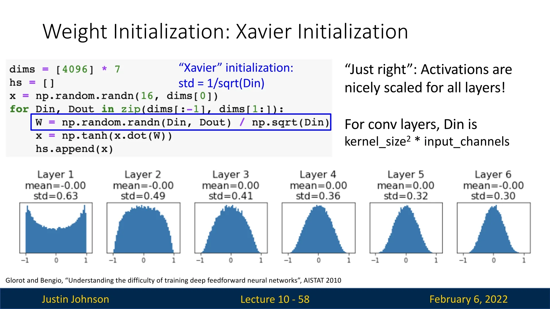
9.4.4 Xavier Initialization
The Xavier Initialization (also known as Glorot Initialization), proposed by Glorot and Bengio [184], is one of the foundational variance-based initialization techniques in deep learning. Its goal is to maintain stable signal propagation—ensuring that both activations and gradients preserve a consistent scale across layers. This approach is especially effective for networks with symmetric activation functions (e.g., sigmoid, tanh), but less suited to asymmetric rectifiers such as ReLU, which require a different scaling strategy (addressed later with Kaiming initialization).
Motivation
For deep networks to train effectively, information must propagate through many layers without numerical or statistical distortion. Ideally, both activations (forward signals) and gradients (backward signals) should maintain consistent magnitudes across depth—neither exploding nor vanishing. If activations grow layer by layer, they saturate nonlinearities and destabilize gradients; if they decay, neurons receive near-zero inputs, halting learning.
To prevent this, weight initialization must ensure that the variance of signals remains approximately constant in both directions of propagation: \[ \operatorname {Var}[s^i] \approx \operatorname {Var}[s^{i-1}], \qquad \operatorname {Var}\!\left [\frac {\partial \mathcal {L}}{\partial s^i}\right ] \approx \operatorname {Var}\!\left [\frac {\partial \mathcal {L}}{\partial s^{i+1}}\right ]. \] The first condition preserves the dynamic range of activations in the forward pass, while the second keeps gradient magnitudes stable during backpropagation. When both hold, each layer transmits information with a unit signal gain, preventing cumulative distortion as depth increases.
The central idea of Xavier Initialization is to analytically determine the appropriate weight variance \( \operatorname {Var}[W^i] \) that simultaneously satisfies these two requirements under reasonable statistical assumptions about the data and activation function. This principle—balancing forward and backward variance—forms the mathematical core of variance-preserving initialization schemes.
Mathematical Formulation
Consider a fully connected layer that transforms input activations \( z^{i-1} \in \mathbb {R}^{n^{i-1}} \) into output activations \( z^{i} \in \mathbb {R}^{n^{i}} \): \[ s^{i} = z^{i-1} W^{i} + b^{i}, \qquad z^{i} = f(s^{i}), \] where \( W^{i} \in \mathbb {R}^{n^{i-1} \times n^{i}} \) is the weight matrix, \( b^{i} \in \mathbb {R}^{n^{i}} \) the bias vector, and \( f(\cdot ) \) a nonlinear activation function applied element-wise.
At initialization, we seek a choice of \( \operatorname {Var}[W^{i}] \) that maintains stable variance through the network: \[ \operatorname {Var}[s^{i}] = \operatorname {Var}[s^{i-1}] = \mbox{constant}. \] Since each pre-activation \( s^{i}_k = \sum _j W^{i}_{j,k} z^{i-1}_j + b^{i}_k \) aggregates \( n^{i-1} \) independent inputs, its variance can be expressed as a function of the fan-in, fan-out, and activation statistics. By equating forward and backward variance terms, Xavier initialization derives an optimal scaling factor for \( \operatorname {Var}[W^{i}] \), yielding weights that preserve signal magnitude in both passes. This derivation follows under the assumptions detailed next.
Assumptions
The derivation of Xavier initialization relies on the following key assumptions:
-
Assumption 1: The activation function is odd with a unit derivative at 0. This means that: \begin {equation} f^{\prime }(0) = 1, \quad f(-x) = -f(x). \end {equation} This assumption is satisfied by the tanh function but not by ReLU, which does not have a well-defined derivative at 0.
- Assumption 2: Inputs, weights, and biases at initialization are independently and identically distributed (iid). This ensures that no correlation skews the variance calculations.
- Assumption 3: Inputs are normalized to have zero mean, and the weights and biases are initialized from a distribution centered at 0. This implies: \begin {equation} \mathbb {E}\left [z^0\right ] = \mathbb {E}\left [W^i\right ] = \mathbb {E}\left [b^i\right ] = 0. \end {equation}
Given these assumptions, we proceed to derive the initialization method.
Derivation of Xavier Initialization
The derivation of Xavier initialization is based on analyzing how variance propagates through both the forward and backward passes of a neural network. The goal is to ensure that the variance of activations and gradients remains stable across layers, preventing vanishing or exploding signals during training. A more detailed step-by-step derivation can be found in [231]. Here, we summarize the key results.
Forward Pass: Maintaining Activation Variance In the forward pass, the activations at layer \( i \) are computed as: \begin {equation} s^i = z^{i-1} W^i + b^i. \end {equation} Applying the activation function \( f(\cdot ) \), we obtain: \begin {equation} z^i = f(s^i). \end {equation}
Our objective is to ensure that the variance of activations remains constant across layers: \begin {equation} \operatorname {Var}[z^i] = \operatorname {Var}[z^{i-1}]. \end {equation} To analyze this, we assume that \( z^{i-1} \) and \( W^i \) are independent and zero-centered, giving: \begin {equation} \operatorname {Var}[s^i] = \operatorname {Var}[z^{i-1} W^i] = n^{i-1} \operatorname {Var}[W^i] \operatorname {Var}[z^{i-1}]. \end {equation}
Setting \( \operatorname {Var}[z^i] = \operatorname {Var}[z^{i-1}] \), we solve for \( \operatorname {Var}[W^i] \):
\begin {equation} \operatorname {Var}[W^i] = \frac {1}{n^{i-1}}. \end {equation}
This means that choosing weights with this variance (depending on the number of neurons in the previous layer \(n^{i-1}\), for each layer \(i\)) ensures that the activations do not shrink or explode as they propagate through the network.
Backward Pass: Maintaining Gradient Variance During backpropagation, the gradient of the loss function with respect to the pre-activation \( s^i \) at layer \( i \) is given by: \begin {equation} \frac {\partial \operatorname {Cost}}{\partial s^i} = \frac {\partial \operatorname {Cost}}{\partial z^i} f'(s^i). \end {equation} The gradients are then propagated backward using: \begin {equation} \frac {\partial \operatorname {Cost}}{\partial z^{i-1}} = W^i \frac {\partial \operatorname {Cost}}{\partial s^i}. \end {equation}
To ensure stable gradient flow, we want to maintain constant variance across layers: \begin {equation} \operatorname {Var} \left ( \frac {\partial \operatorname {Cost}}{\partial s^i} \right ) = \operatorname {Var} \left ( \frac {\partial \operatorname {Cost}}{\partial s^{i+1}} \right ). \end {equation}
Since \( W^i \) and \( \frac {\partial \operatorname {Cost}}{\partial s^i} \) are independent and zero-centered, we get:
\begin {equation} \operatorname {Var} \left ( \frac {\partial \operatorname {Cost}}{\partial s^i} \right ) = n^i \operatorname {Var}[W^i] \operatorname {Var} \left ( \frac {\partial \operatorname {Cost}}{\partial s^{i+1}} \right ). \end {equation}
Setting \( \operatorname {Var} \left ( \frac {\partial \operatorname {Cost}}{\partial s^i} \right ) = \operatorname {Var} \left ( \frac {\partial \operatorname {Cost}}{\partial s^{i+1}} \right ) \), we solve for \( \operatorname {Var}[W^i] \):
\begin {equation} \operatorname {Var}[W^i] = \frac {1}{n^i}. \end {equation}
This ensures that the gradients do not shrink or explode as they propagate backward.
Balancing Forward and Backward Variance The variance conditions obtained from the forward and backward pass derivations are: \begin {equation} \operatorname {Var}[W^i] = \frac {1}{n^{i-1}}, \quad \mbox{(from forward pass)} \end {equation} \begin {equation} \operatorname {Var}[W^i] = \frac {1}{n^i}, \quad \mbox{(from backward pass)} \end {equation}
These two conditions are equal only when \( n^{i-1} = n^i \), meaning all layers have the same number of neurons. However, in most architectures, layers do not have identical sizes, making it impossible to satisfy both conditions simultaneously.
To resolve this, Glorot and Bengio proposed taking the average of the two results:
\begin {equation} \operatorname {Var}[W^i] = \frac {2}{n^{i-1} + n^i}. \end {equation}
This balances the variance of activations and gradients across layers. Although it isn’t proven/guaranteed that this initialization will work, in practice it appears to usually work, making this a common weight initialization approach.
Final Xavier Initialization Formulation
The final Xavier initialization scheme follows the computed variance. The weights are sampled from either:
- A normal distribution: \begin {equation} W^i \sim \mathcal {N} \left ( 0, \frac {2}{n^{i-1} + n^i} \right ). \end {equation}
- A uniform distribution: \begin {equation} W^i \sim U \left ( -\sqrt {\frac {6}{n^{i-1} + n^i}}, \sqrt {\frac {6}{n^{i-1} + n^i}} \right ). \end {equation}
These choices ensure stable propagation of activations and gradients, improving the convergence of deep networks.
Limitations of Xavier Initialization
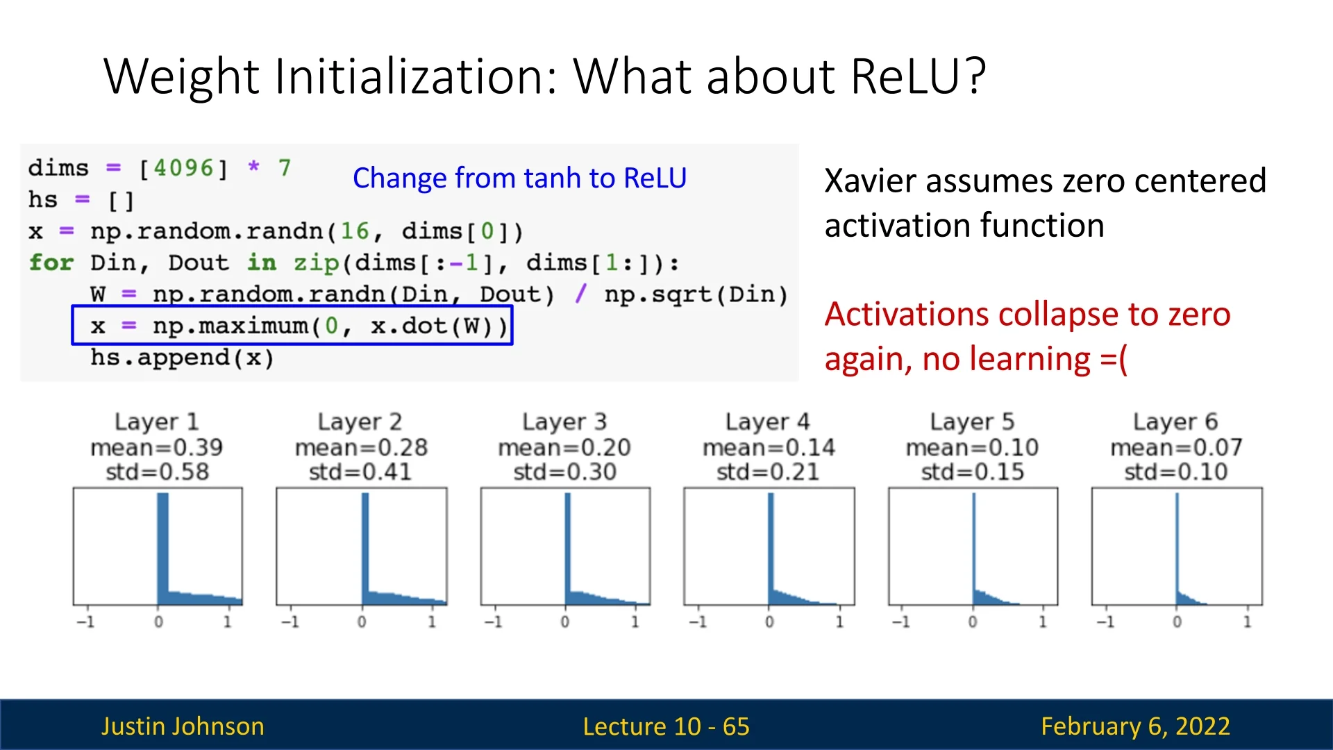
While Xavier initialization improves stability in training deep networks, it is primarily suited for activations like sigmoid and tanh. However, for ReLU-based networks, which are more common nowadays as ReLU and its variants are more suitable activation functions for deep learning, as they do not satisfy the odd symmetry assumption, a different method—Kaiming He Initialization is more appropriate [216].
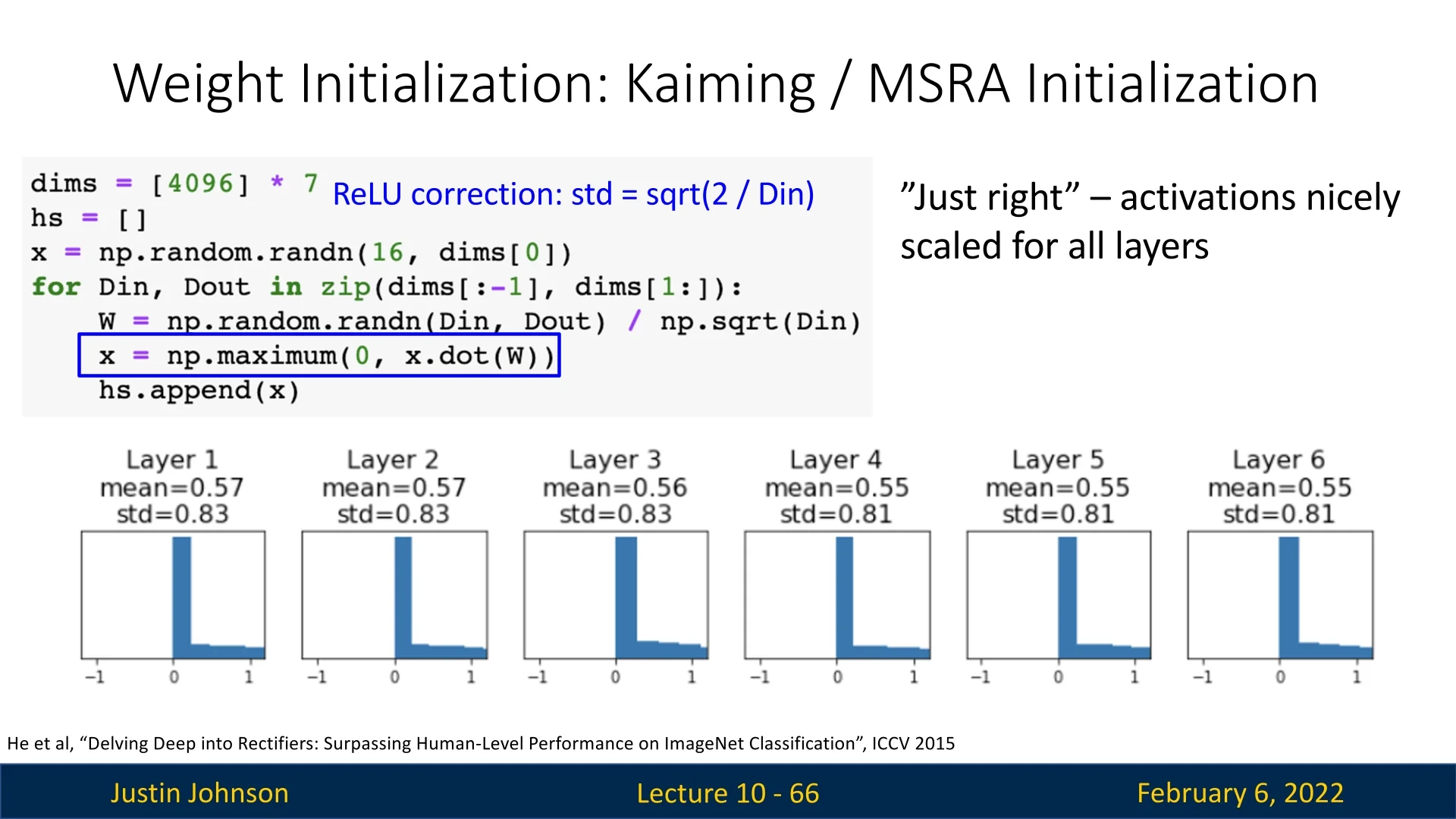
9.4.5 Kaiming He Initialization
Xavier initialization was derived assuming symmetric activation functions such as tanh and sigmoid. However, modern deep networks frequently use ReLU and its variants, which introduce asymmetry due to their non-negative outputs. To address this, Kaiming He initialization [216] was designed specifically for ReLU-based networks.
A more detailed mathematical derivation can be found in [230]. Here, we summarize the key results.
Motivation
The ReLU function is defined as: \begin {equation} \operatorname {ReLU}(x) = \max (0, x). \end {equation} Unlike tanh or sigmoid, ReLU has a zero-negative property, meaning half of the activations become zero. This effectively reduces the variance of activations by a factor of \( 2 \), requiring an adjustment in the weight initialization.
Similar to Xavier initialization, the goal is to ensure stable variance across both forward and backward passes while considering ReLU’s characteristics.
Mathematical Notation We define a neural network layer with the following variables:
- Weight matrix: \( W_k \in \mathbb {R}^{n_k \times n_{k+1}} \)
- Bias vector: \( b_k \in \mathbb {R}^{n_{k+1}} \)
- Input activations: \( x_k \in \mathbb {R}^{n_k} \)
- Pre-activation outputs: \( y_k = x_k W_k + b_k \)
- Post-activation outputs: \( x_{k+1} = f(y_k) \), where \( f(x) \) is the ReLU activation function.
- The network’s loss function is denoted by \( L \).
- Gradients of the loss function w.r.t. activations: \( \Delta x_k = \frac {\partial L}{\partial x_k} \).
Assumptions
The derivation relies on the following key assumptions:
- 1.
- ReLU activation: Defined as: \begin {equation} f(x) = \operatorname {ReLU}(x) = \max (0, x), \end {equation} with its derivative: \begin {equation} f'(x) = \begin {cases} 1, & x > 0 \\ 0, & x \leq 0. \end {cases} \end {equation} This means that, on average, only half of the inputs contribute to the signal.
- 2.
- Independent and identically distributed (iid) initialization: Inputs, weights, and gradients are assumed to be iid at initialization.
- 3.
- Zero-mean initialization: Inputs and weights are drawn from a zero-centered distribution: \begin {equation} \mathbb {E}[x_0] = \mathbb {E}[W_k] = \mathbb {E}[b_k] = 0. \end {equation}
Forward and Backward Pass Derivation
To determine an appropriate variance for weight initialization, we ensure that variance remains stable across layers during both forward and backward propagation. If the variance is too high, activations and gradients explode, leading to instability. If it is too low, activations and gradients vanish, slowing down learning.
The challenge with ReLU is that it sets all negative inputs to zero, effectively discarding half of the activation values. This requires adjusting the variance to prevent it from shrinking as it propagates through layers.
Forward Pass Analysis The goal is to determine the weight variance that maintains constant variance across layers during forward propagation: \begin {equation} \operatorname {Var}[y_k] = \operatorname {Var}[y_{k-1}]. \end {equation}
Since the transformation follows: \begin {equation} y_k = x_k W_k + b_k, \end {equation} applying the variance operator:
\begin {equation} \operatorname {Var}[y_k] = \operatorname {Var}[x_k W_k] + \operatorname {Var}[b_k]. \end {equation}
Assuming \( b_k = 0 \) at initialization: \begin {equation} \operatorname {Var}[y_k] = \operatorname {Var}[x_k W_k]. \end {equation}
Given independence between \( x_k \) and \( W_k \): \begin {equation} \operatorname {Var}[y_k] = n_k \operatorname {Var}[W_k] \operatorname {Var}[x_k]. \end {equation}
Since ReLU eliminates half the activations, the expected variance is: \begin {equation} \operatorname {Var}[x_k] = \frac {1}{2} \operatorname {Var}[y_{k-1}]. \end {equation}
Substituting this: \begin {equation} \operatorname {Var}[y_k] = n_k \operatorname {Var}[W_k] \frac {1}{2} \operatorname {Var}[y_{k-1}]. \end {equation}
Setting \( \operatorname {Var}[y_k] = \operatorname {Var}[y_{k-1}] \): \begin {equation} \operatorname {Var}[W_k] = \frac {2}{n_k}. \end {equation}
Backward Pass Analysis Similar reasoning applies to backpropagation, ensuring that gradient variance remains stable: \begin {equation} \operatorname {Var}[\Delta x_k] = \operatorname {Var}[\Delta x_{k+1}]. \end {equation}
The gradient follows: \begin {equation} \Delta x_k = \Delta y_k W_k^T. \end {equation}
Applying the variance operator: \begin {equation} \operatorname {Var}[\Delta x_k] = \operatorname {Var}[\Delta y_k W_k^T]. \end {equation}
Using independence: \begin {equation} \operatorname {Var}[\Delta x_k] = n_k \operatorname {Var}[W_k] \operatorname {Var}[\Delta y_k]. \end {equation}
ReLU’s gradient is 1 for positive inputs and 0 otherwise: \begin {equation} \operatorname {Var}[\Delta y_k] = \frac {1}{2} \operatorname {Var}[\Delta x_{k+1}]. \end {equation}
Substituting: \begin {equation} \operatorname {Var}[\Delta x_k] = n_k \operatorname {Var}[W_k] \frac {1}{2} \operatorname {Var}[\Delta x_{k+1}]. \end {equation}
Setting \( \operatorname {Var}[\Delta x_k] = \operatorname {Var}[\Delta x_{k+1}] \): \begin {equation} \operatorname {Var}[W_k] = \frac {2}{n_k}. \end {equation}
Final Kaiming Initialization Formulation
Unlike Xavier initialization, which averages forward and backward variance conditions, Kaiming He initialization naturally satisfies both simultaneously due to the ReLU-specific factor of \( 2 \). The final weight initialization is:
- Normal distribution: \begin {equation} W_k \sim \mathcal {N} \left ( 0, \frac {2}{n_k} \right ). \end {equation}
- Uniform distribution: \begin {equation} W_k \sim U \left ( -\sqrt {\frac {6}{n_k}}, \sqrt {\frac {6}{n_k}} \right ). \end {equation}
Implementation in Deep Learning Frameworks
Kaiming He initialization is widely supported in deep learning libraries such as PyTorch:
import torch.nn as nn
nn.init.kaiming_uniform_(layer.weight, mode=’fan_in’, nonlinearity=’relu’)
For normal distribution:
nn.init.kaiming_normal_(layer.weight, mode=’fan_in’, nonlinearity=’relu’)This method ensures stable variance and effective training for ReLU-based deep networks.
Initialization in Residual Networks (ResNets)
Residual Networks (ResNets) introduce skip connections, which allow the network to learn residual functions instead of direct mappings. While this architectural design helps address vanishing gradients, it also violates the assumptions of Kaiming (MSRA) initialization [216].
Why Doesn’t Kaiming Initialization Work for ResNets? In standard Kaiming initialization, the goal is to maintain a stable variance across layers, ensuring that: \begin {equation} \operatorname {Var}[F(x)] = \operatorname {Var}[x]. \end {equation} However, in ResNets, the output of each block is computed as: \begin {equation} x_{l+1} = x_l + F(x_l), \end {equation} where \( F(x_l) \) is the residual mapping.
If we apply Kaiming initialization naively, we get: \begin {equation} \operatorname {Var}[x_{l+1}] = \operatorname {Var}[x_l] + \operatorname {Var}[F(x_l)]. \end {equation} Since \( \operatorname {Var}[F(x_l)] = \operatorname {Var}[x_l] \), this leads to: \begin {equation} \operatorname {Var}[x_{l+1}] = 2 \operatorname {Var}[x_l]. \end {equation} This causes the variance to grow with each residual block, leading to exploding activations and gradients, which disrupts training.
Fixup Initialization To address this issue, Fixup Initialization [790] proposes a modification to the initialization strategy:
- The first convolutional layer in each residual block is initialized using Kaiming (MSRA) initialization.
- The second convolutional layer in the residual block is initialized to zero.
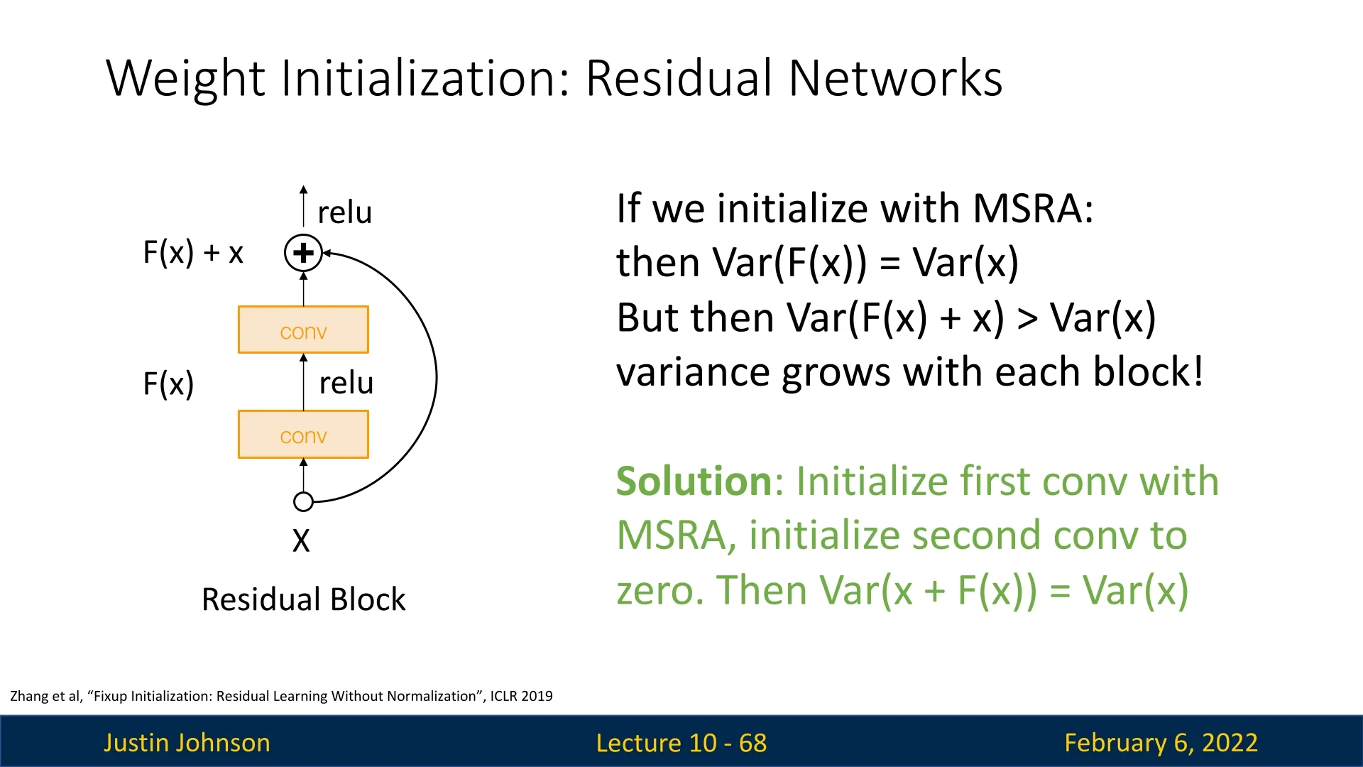
This ensures that at initialization: \begin {equation} \operatorname {Var}[x_{l+1}] = \operatorname {Var}[x_l], \end {equation} meaning the variance remains stable across layers at the start of training.
This simple adjustment ensures that deep ResNets can be trained effectively without batch normalization or layer normalization, making Fixup particularly useful in certain settings.
9.4.6 Conclusion: Choosing the Right Initialization Strategy
Weight initialization plays a critical role in stabilizing training dynamics, preventing vanishing or exploding gradients, and improving optimization efficiency in deep neural networks. The choice of initialization depends on the network architecture and the activation functions used. Below, we summarize the most widely adopted initialization strategies and their appropriate use cases:
- Xavier (Glorot) Initialization [184]: Best suited for networks using symmetric activation functions such as tanh or sigmoid, where maintaining equal variance across layers is crucial.
- Kaiming (He) Initialization [216]: Specifically designed for ReLU and its variants (Leaky ReLU, PReLU, etc.), accounting for their asymmetric nature by scaling variance accordingly to prevent dying neurons.
- Fixup Initialization [790]: Designed for Residual Networks (ResNets), where skip connections alter the variance accumulation dynamics, requiring an adaptation of Kaiming initialization to prevent activation and gradient explosion.
- T-Fixup Initialization [258]: Developed for Transformer models, which do not use batch normalization and suffer from unstable training due to layer normalization effects. T-Fixup provides an alternative scaling strategy that allows deep Transformers to be trained without learning rate warm-up.
Ongoing Research and Open Questions
While the above techniques are widely used, weight initialization remains an active area of research due to several challenges:
- Deeper Architectures: As networks grow deeper, traditional initialization methods may become insufficient. Methods such as Scaled Initialization [53] and Dynamically Normalized Initialization are being explored.
- Transformers and Non-Convolutional Architectures: Transformers and other architectures differ significantly from CNN-based models, requiring specialized initialization strategies such as T-Fixup.
- Self-Supervised Learning and Sparse Networks: Recent advances in sparse training and self-supervised learning suggest that certain initialization methods may benefit from adjustments tailored to these paradigms.
- Adaptive Initialization: Some research explores dynamically adjusting initialization during training instead of relying on fixed heuristics.
Weight initialization remains a crucial component of deep learning optimization. While methods like Kaiming and Fixup work well for standard deep networks, ongoing research continues to refine initialization strategies for emerging architectures. The field is evolving toward more specialized and adaptive initialization schemes to address challenges posed by depth, architecture type, and optimization dynamics.
9.5 Regularization Techniques
We have previously discussed L1/L2 regularization (weight decay) and how batch normalization (BN) can act as an implicit regularizer. However, in some cases (usually with less modern architectures, like VGG or AlexNet), these methods are insufficient to prevent overfitting. In such cases, even when a model successfully fits the training data, it may generalize poorly to unseen test samples (hence, over-fitting). This issue is typically observed when the validation loss increases while the training loss continues to decrease during training.
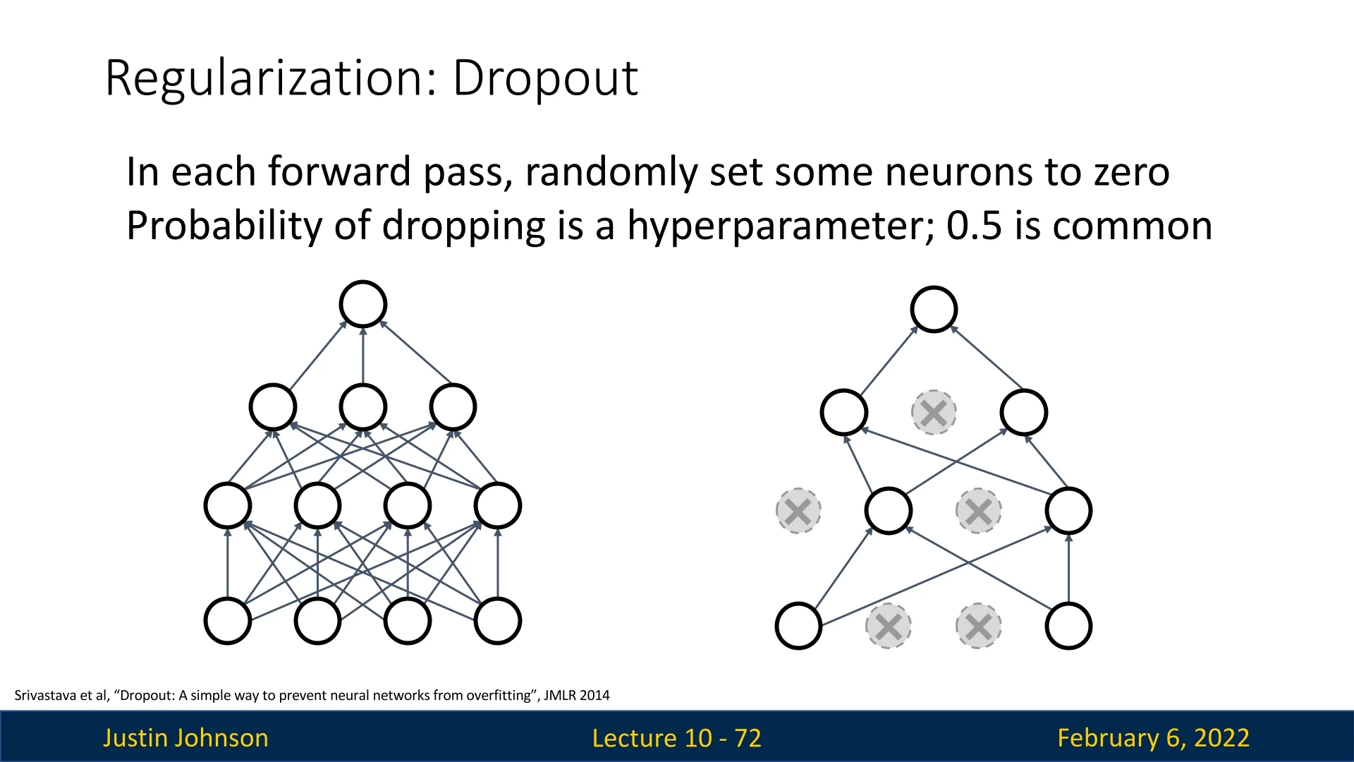
9.5.1 Dropout
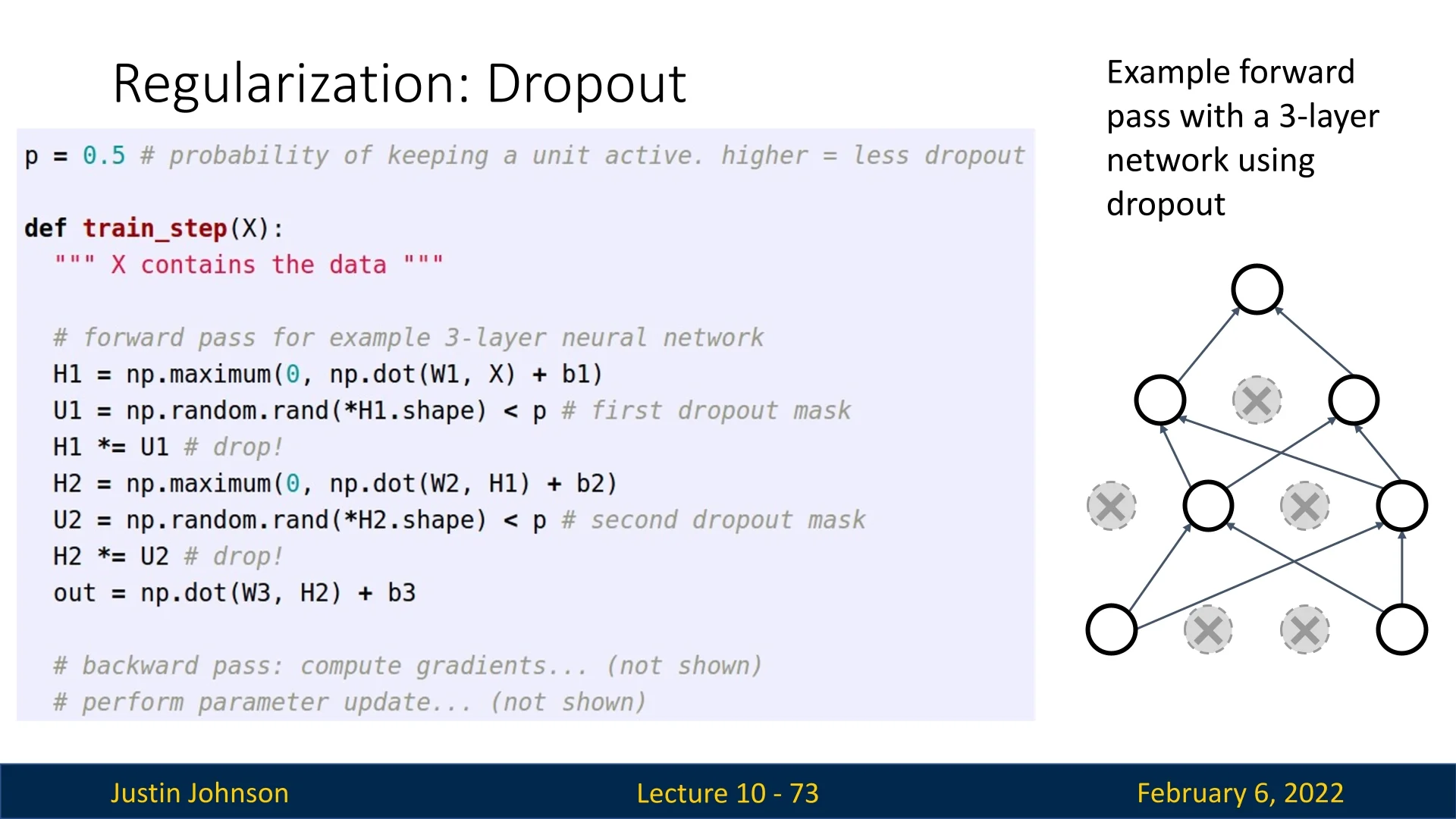
A widely used regularization technique to combat overfitting is dropout [607]. The key idea behind dropout is to randomly set some neurons in each layer to zero during the forward pass, with a probability \( p \) (commonly set to \( 0.5 \)). This stochastic behavior forces the network to learn redundant representations, improving generalization.
Dropout is simple to implement and has proven to be an effective regularization method in deep networks.
Why Does Dropout Work?
One way to understand the effectiveness of dropout is by considering its impact on feature representation learning. By forcing the network to function even when certain neurons are randomly deactivated, dropout encourages the learning of multiple redundant representations, reducing the reliance on specific neurons or sets of neurons. This helps prevent co-adaptation of features, resulting in more robust and generalizable representations.
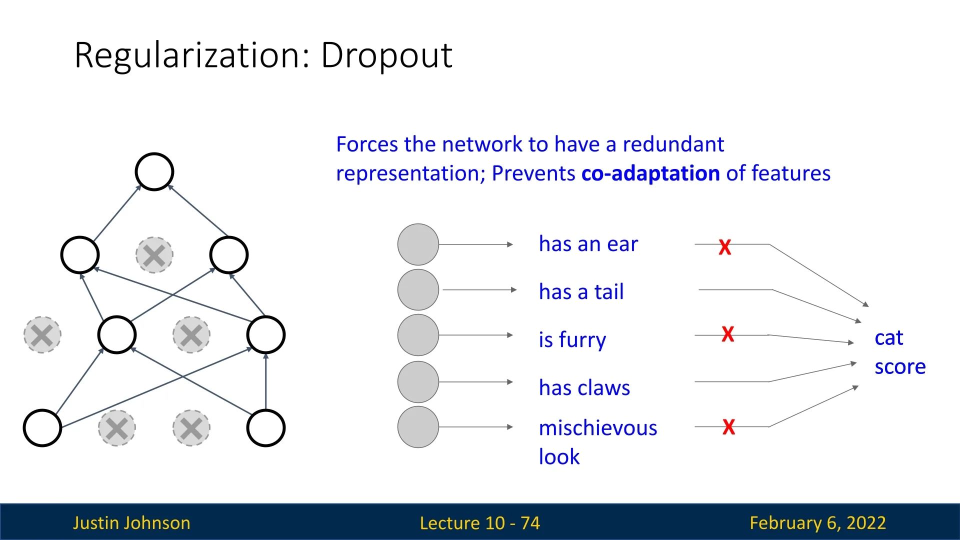
Consider a classification network trained to recognize cats. Without dropout, the network may learn to identify a cat based on a small, specific set of neurons that respond to features such as ”has whiskers” or ”has pointy ears.” If these neurons fail to activate (e.g., due to occlusion in an image), the model may fail to classify the image correctly.
With dropout, the network is forced to distribute its learned representations across multiple neurons. For instance, one subset of neurons may respond to features such as ”has a tail” and ”is furry”, while another may respond to ”has whiskers” and ”has claws.” Because dropout randomly deactivates neurons during training, the network learns to rely on multiple sets of features instead of a single subset. This redundancy ensures that even if some neurons are missing at test time, the network still has enough information to classify the image correctly.
In essence, dropout forces the model to learn diverse and distributed feature representations, making it more robust to missing or occluded features in unseen images.
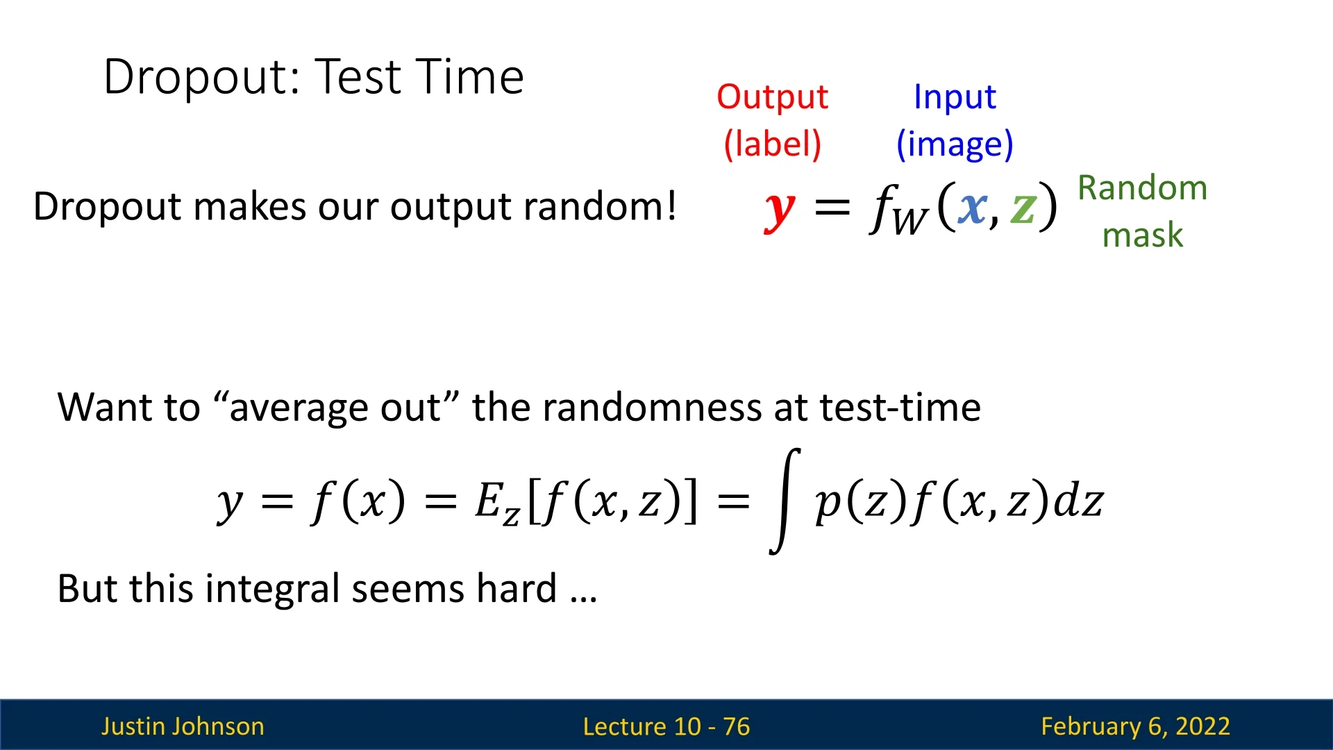
Dropout at Test Time
During training, dropout introduces randomness into the network, which is beneficial for regularization. However, at test time, we require a deterministic model to ensure consistent and reliable predictions. If we were to apply dropout at test time, different subsets of neurons would be randomly deactivated on each forward pass, making the model’s output highly inconsistent.
Why is a stochastic model at inference problematic? Consider an autonomous vehicle that uses a neural network to recognize traffic signs. If dropout were applied at test time, different neurons could be randomly dropped with each forward pass. As a result, the model might predict ”Stop Sign” on one pass and ”Speed Limit 60” on another, leading to highly inconsistent and potentially dangerous decisions.
Another example is medical diagnosis. Suppose a deep learning model is used to analyze medical images for detecting tumors. If dropout were applied at test time, the model’s prediction for the presence of a tumor might vary between different forward passes. A doctor using the model would see conflicting results, making it impossible to rely on the system for accurate medical diagnoses.
To prevent this, we rewrite the network as a function of two inputs: the input tensor \( x \) and a random binary mask \( z \), drawn from a predefined probability distribution:
\begin {equation} y = f(x, z). \end {equation}
To obtain a stable output at test time, we seek the expected value of \( y \), marginalized over all possible values of \( z \):
\begin {equation} \mathbb {E}_z[f(x, z)] = \int p(z) f(x, z) dz. \end {equation}
However, computing this integral analytically is infeasible in practice, requiring an approximation.
Consider a single neuron receiving two inputs \( x \) and \( y \) with corresponding weights \( w_1 \) and \( w_2 \). During training, with dropout probability \( p = 0.5 \), the expected activation is:
\begin {equation} \mathbb {E}[a] = \frac {1}{4} (w_1 x + w_2 y) + \frac {1}{4} (w_1 x + 0y) + \frac {1}{4} (0x + 0y) + \frac {1}{4} (0x + w_2 y). \end {equation}
Simplifying, we obtain:
\begin {equation} \mathbb {E}[a] = \frac {1}{2} (w_1 x + w_2 y). \end {equation}
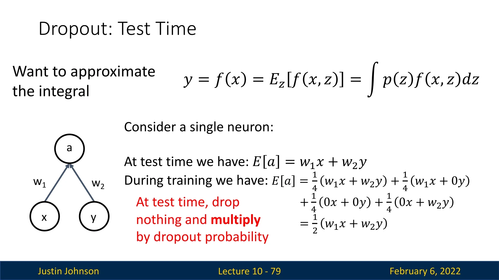
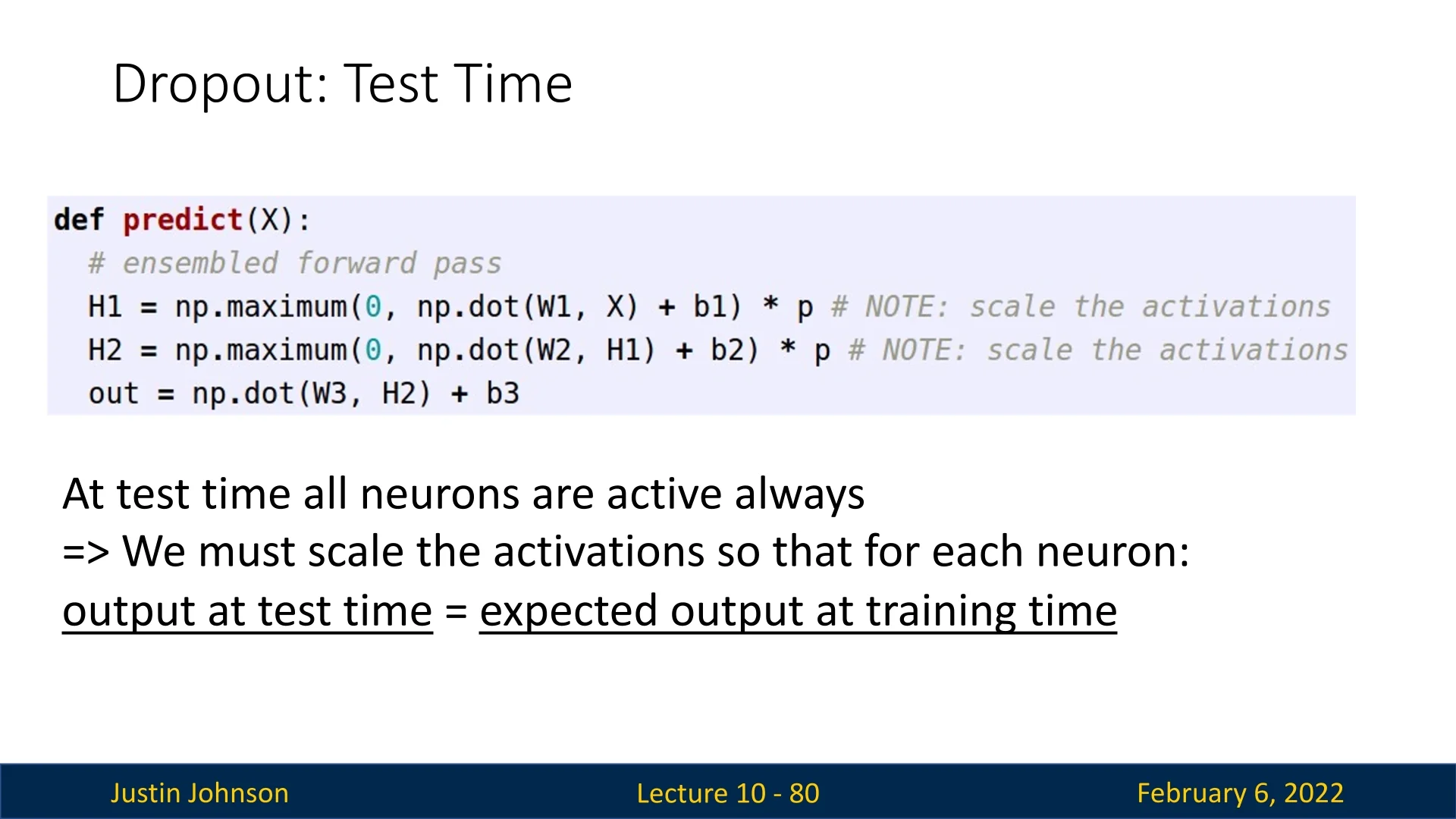
Generalizing this result, at test time, we compensate for the randomness introduced during training by scaling each output by the dropout probability \( p \). That is, at test time, all neurons are active, but their activations are scaled by \( p \) to match the expected output seen during training.
Inverted Dropout
A more common implementation of dropout, known as inverted dropout, simplifies the test-time scaling process by incorporating it into training. Instead of scaling activations at test time, we scale them during training. This is achieved by dividing the retained activations by \( p \) during training, ensuring that the expected activations at test time remain the same without any need for post-processing.
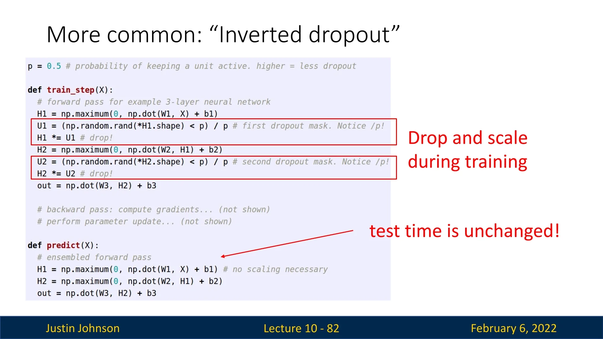
Formally, during training:
\begin {equation} a' = \frac {a}{p}. \end {equation}
At test time, all neurons remain active, and no additional scaling is required.
Where is Dropout Used in CNNs?
In early CNN architectures such as AlexNet and VGG16, fully connected layers (MLPs) were stacked at the end of the network. Dropout was commonly applied to these layers to prevent overfitting. However, in modern architectures, fully connected layers have been largely replaced by global average pooling (GAP) followed by a single fully connected layer. This transition has made dropout less commonly used in CNNs.
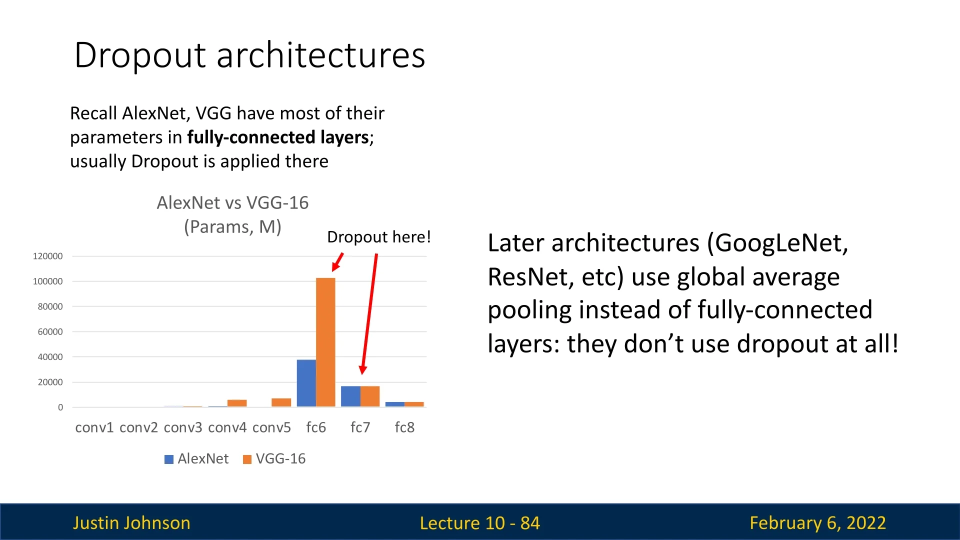
Back in 2014, Dropout was an essential component for training neural networks, often succeeding in reducing overfitting, allowing deeper models to train and provide improved results over shallower ones. While dropout remains a useful technique in some deep networks, its necessity has diminished in architectures that rely less on FC layers, or ones incorporating other alternative regularization mechanisms.
Enrichment 9.5.2: Ordering of Dropout and Batch Normalization
Dropout and Batch Normalization (BN) are commonly used regularization techniques, but their order in the computational pipeline affects their effectiveness. This section examines the impact of their ordering and why BN is typically placed before Dropout.
Enrichment 9.5.2.1: Impact of Dropout Placement on BN
The placement of Dropout relative to Batch Normalization (BN) can significantly affect training stability and performance. If Dropout is applied before BN, it modifies activations stochastically, leading to inconsistent batch statistics: \[ \mu _B = \mathbb {E}[\mathbf {m} \odot \mathbf {u}], \quad \sigma _B^2 = \mathbb {E}[(\mathbf {m} \odot \mathbf {u})^2] - \mathbb {E}[\mathbf {m} \odot \mathbf {u}]^2. \] Here, \(\mathbf {m}\) is a binary mask sampled independently per batch. Since different neurons are randomly dropped each forward pass, the estimated mean \(\mu _B\) and variance \(\sigma _B^2\) fluctuate across iterations, affecting BN’s ability to normalize effectively. This results in:
- Unstable batch statistics: BN normalizes activations using batch-wide estimates of \(\mu _B, \sigma _B^2\). With Dropout applied first, the expected value of activations varies unpredictably due to random masking, introducing variance into these estimates. Mathematically, since \(\mathbb {E}[\mathbf {m}] = p\), where \(p\) is the Dropout retention probability, BN effectively normalizes over \(\mathbf {m} \odot \mathbf {u}\), distorting the expected statistics.
- Inconsistent normalization: BN aims to stabilize activations across training by ensuring a consistent distribution. However, when Dropout precedes BN, the latter adapts to a distribution affected by stochastic sparsity rather than the actual underlying feature distribution, leading to erratic normalization behavior.
- Reduced Dropout effectiveness: BN rescales activations based on mini-batch statistics. If Dropout zeros out activations before BN, BN may adjust its normalization parameters such that previously zeroed activations are shifted back to nonzero values. This undermines Dropout’s intended function of inducing sparsity and reducing co-adaptation between neurons.
Enrichment 9.5.2.2: Why BN Before Dropout is Preferred
To maintain stable normalization while preserving Dropout’s regularization benefits, BN should be applied before Dropout:
\[ \mathbf {x} \;\xrightarrow {\quad \mathrm {Linear}\quad }\; \mathbf {u} \;\xrightarrow {\quad \mathrm {BN}\quad }\; \widehat {\mathbf {u}} \;\xrightarrow {\quad \phi (\cdot )\quad }\; \mathbf {z} \;\xrightarrow {\quad \mathrm {Dropout}\quad }\; \mathbf {\tilde {z}}. \]
This ordering ensures:
- Reliable batch statistics: BN operates on unperturbed pre-activations, maintaining consistent estimates of \(\mu _B, \sigma _B^2\). Since BN relies on these running statistics for inference, applying it before Dropout prevents artificially induced variance that could degrade model stability.
- Preserved Dropout effect: Dropout is applied after BN, ensuring that zeroed activations remain zeroed, rather than being rescaled. This allows Dropout to function as intended, improving regularization without interference from BN’s normalization step.
- Smoother convergence: When Dropout follows BN, the added stochasticity occurs after stable normalization, preventing erratic gradient updates while still regularizing the network.
The optimal placement of BN and Dropout can vary depending on the network architecture and task:
- In CNNs, Dropout may be omitted entirely since BN alone can sufficiently regularize.
- In Transformers, Dropout is typically applied to attention weights.
- In large-scale datasets (e.g., ImageNet [265]), Dropout is often used only in deeper layers where BN alone may not provide enough regularization.
9.5.2 Other Regularization Techniques
The idea behind dropout introduces a common pattern seen in various regularization techniques:
- Training: Introduce some form of randomness (e.g., Dropout with a random binary mask \( z \), where \( y = f_W(x, z) \)).
- Testing: Average out the randomness (sometimes approximately), ensuring stable deterministic predictions: \[ y = f(x) = E_z[f_W(x, z)] = \int p(z) f_W(x, z) \, dz. \]
Batch Normalization (BN) also follows this trend. During training, BN normalizes activations using statistics computed from the mini-batch, making the output of each sample dependent on others in the batch (which are chosen randomly). At test time, BN uses fixed statistics to remove the randomness. Thus, BN also fits into this broader category of techniques that introduce randomness during training but stabilize at test time.
Interestingly, with modern architectures like ResNets and their variants, explicit regularization techniques such as Dropout are often unnecessary. Instead, regularization is typically achieved through weight decay (L2 regularization) and BN.
Data Augmentation as Implicit Regularization
Another form of regularization, often not explicitly classified as such, is data augmentation. It introduces controlled randomness into training data by applying transformations that should not alter the desired output (e.g., for classification, shouldn’t change the class identity). These augmentations expand the effective training set size and help improve generalization.
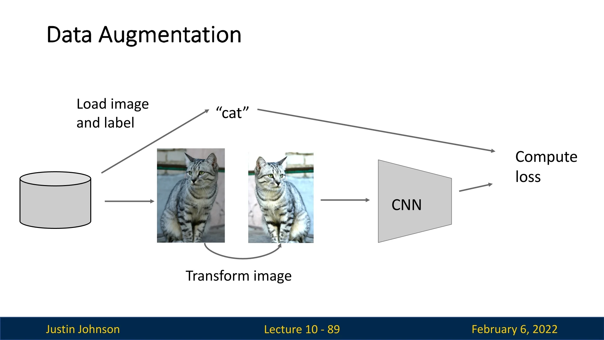
Common augmentation techniques for images include:
- Horizontal flipping (mirroring an image).
- Color jittering (adjusting brightness, contrast, and saturation).
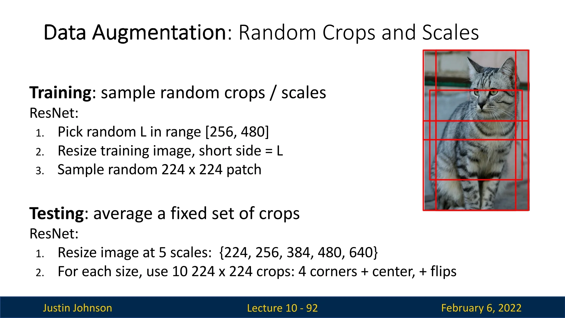
- Random cropping and scaling.
Since augmentations introduce randomness at training time, test-time predictions must be stabilized. One approach is to apply a fixed set of augmentations during inference and average the results.
Augmentation strategies depend on the task and dataset. For example:
- Translation, rotation, shearing, and stretching are useful for robust feature learning.
- Lens distortions may help models adapt to different camera setups.
-
Domain-specific augmentations: Some augmentations are only useful for certain tasks. For example:
- If distinguishing between left and right hands, horizontal flipping should not be applied.
- For classifying cats vs. dogs, flipping is reasonable since a flipped cat/dog is still a cat/dog (class doesn’t change).
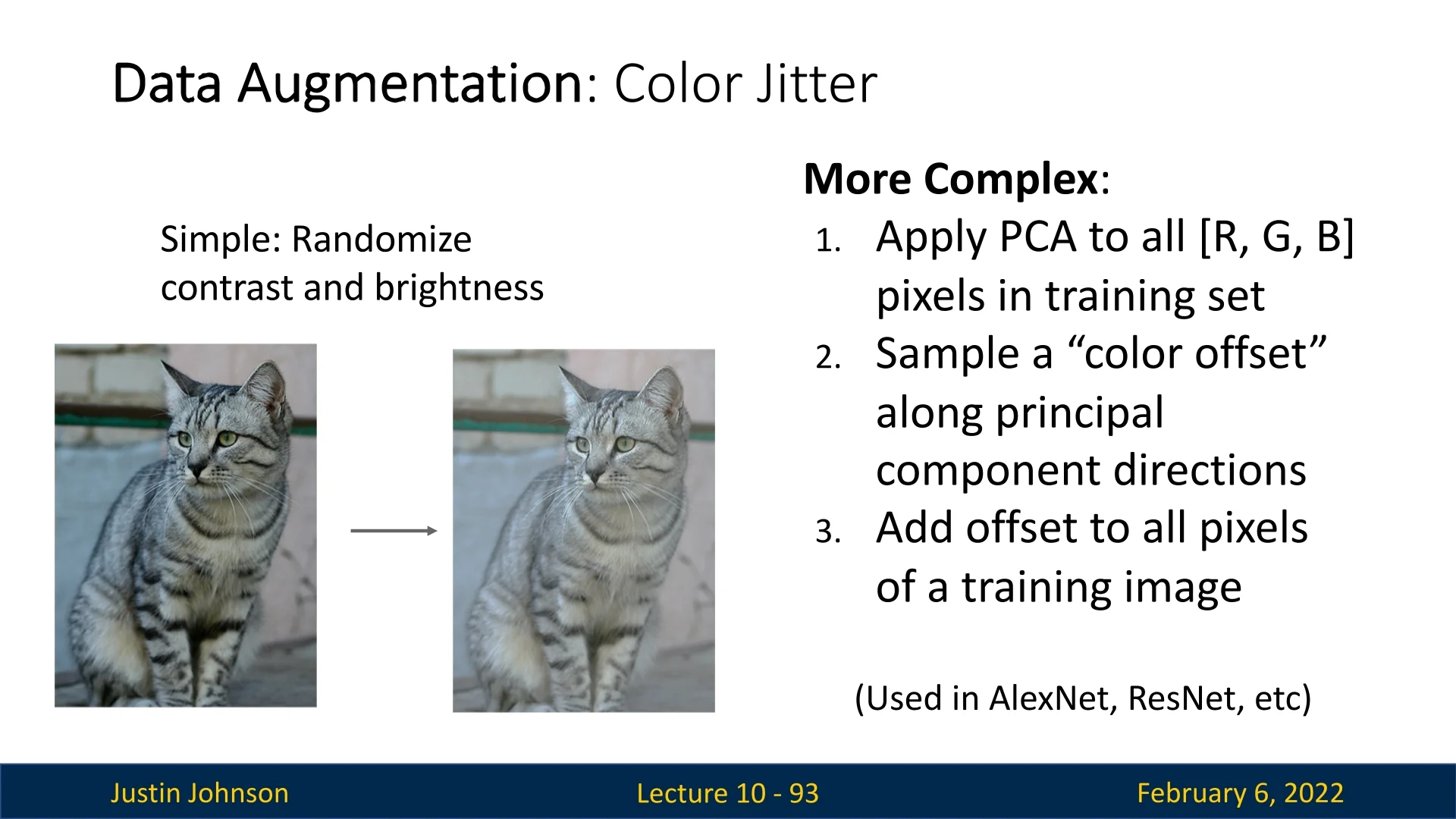
In summary, augmentation is a powerful regularization tool that introduces structured randomness, forcing models to learn robust representations.
DropConnect
DropConnect [675] is a regularization technique similar to Dropout, but instead of randomly setting activations to zero, it randomly drops connections (weights) during the forward pass. This means that rather than deactivating entire neurons, individual weights are set to zero, producing a sparser and more dynamic network during training.
The key equation for DropConnect is:
\begin {equation} y = f((W \odot M) x + b), \end {equation}
where \( M \) is a binary mask with the same shape as \( W \), with entries sampled from a Bernoulli distribution.
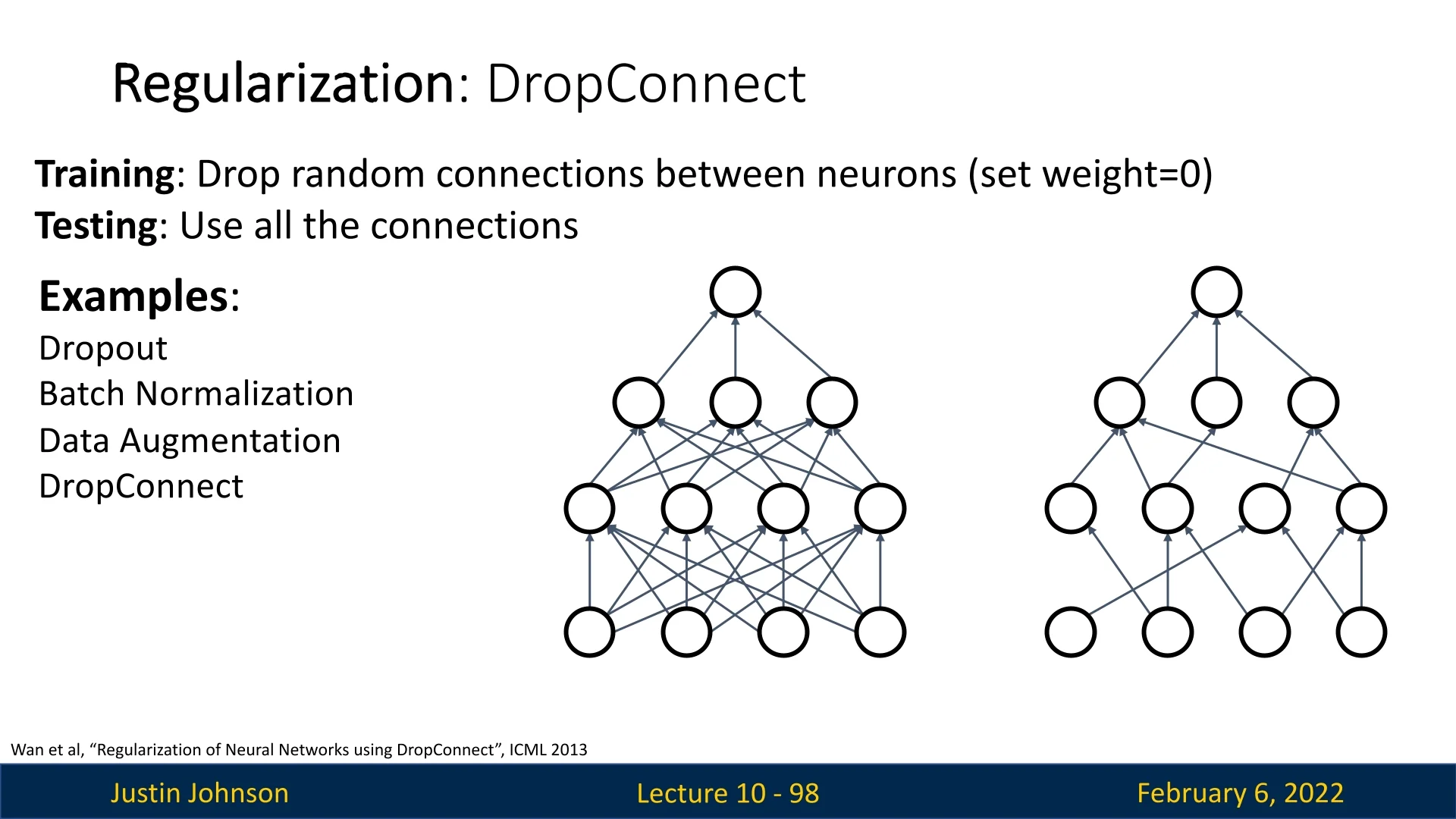
Dropout vs. DropConnect: Comparing Granularities of Randomness
Both Dropout and DropConnect are regularization techniques designed to combat overfitting by introducing stochasticity during training. They both encourage networks to learn robust and redundant representations that do not rely excessively on any single neuron or connection. Their key difference lies in what they randomly disable during training: Dropout removes entire neuron outputs, whereas DropConnect removes individual weights.
Intuitive Analogy Imagine a layer as a team of workers collaborating to complete a complex task:
- Dropout is like randomly telling some workers to take the day off. The remaining team must learn to accomplish the task without them, promoting redundancy and resilience.
- DropConnect, in contrast, keeps all workers on duty but removes a random subset of their tools. Each worker must still perform, but with limited resources, encouraging more distributed and adaptive problem-solving strategies.
This difference in “granularity” fundamentally shapes how each method regularizes the network.
Mechanism and Mathematical View
- Dropout (Neuron-level masking): During training, each neuron’s output activation is set to zero with probability \( p \): \[ a_l^{(i)} \leftarrow a_l^{(i)} \cdot m^{(i)}, \quad m^{(i)} \sim \mbox{Bernoulli}(1 - p). \] This disables entire activations, forcing other neurons in the layer to develop complementary features. Dropout is particularly effective in fully connected layers where neurons tend to co-adapt.
- DropConnect (Weight-level masking): Instead of masking activations, DropConnect randomly sets individual weights to zero before computing pre-activations: \[ z_l^{(i)} = \sum _j \big ( m^{(i,j)} W_l^{(i,j)} a_{l-1}^{(j)} \big ), \quad m^{(i,j)} \sim \mbox{Bernoulli}(1 - p). \] This produces a more fine-grained regularization: each neuron still outputs a value but based on a random subset of its incoming connections. The result is a smoother, more nuanced form of noise injection that preserves partial signal flow.
Effectiveness and Practical Differences
- Dropout: Best suited for dense, fully connected layers or smaller convolutional heads, where deactivating full neurons is an effective way to reduce overfitting. It is simple, efficient, and widely used as a default regularizer in classification networks.
- DropConnect: More appropriate for very deep or heavily parameterized models (e.g., large Transformers or RNNs), where eliminating entire activations would excessively disrupt information flow. By randomly masking individual weights, DropConnect preserves partial contributions while encouraging robustness at a finer scale.
Inference-Time Behavior At test time, both techniques remove randomness and replace it with expected scaling:
- For Dropout, activations are scaled by the retention probability \( (1 - p) \).
- For DropConnect, the same scaling applies to the weights.
Modern implementations often use inverted dropout, performing this scaling during training instead—ensuring inference remains deterministic and efficient.
Summary Dropout and DropConnect share the same goal—improving generalization through stochastic regularization—but differ in their level of intervention:
- Dropout: Coarse-grained; disables entire neuron outputs to break co-adaptation.
- DropConnect: Fine-grained; disables individual weights to enforce distributed, resilient connectivity.
In essence, Dropout acts like “turning off” entire neurons, while DropConnect acts like “cutting random wires” between them. Both prevent overfitting by making the network less dependent on specific units or connections, though DropConnect provides a subtler and often more computationally demanding form of regularization.
Fractional Max Pooling
Traditional max pooling operations in CNNs use fixed receptive field sizes (e.g., \(2 \times 2\) or \(3 \times 3\)) to downsample feature maps. Fractional Max Pooling [189] introduces randomized pooling regions, where the size of the pooling regions varies across different neurons and different forward passes.
Instead of a fixed pooling size, each neuron is assigned a pooling region that is sampled randomly. For example, some neurons may have a \(2 \times 2\) region, while others may have a \(1 \times 1\) region. On average, each neuron receives a fractional pooling region (e.g., \(1.35\) receptive field size on average).
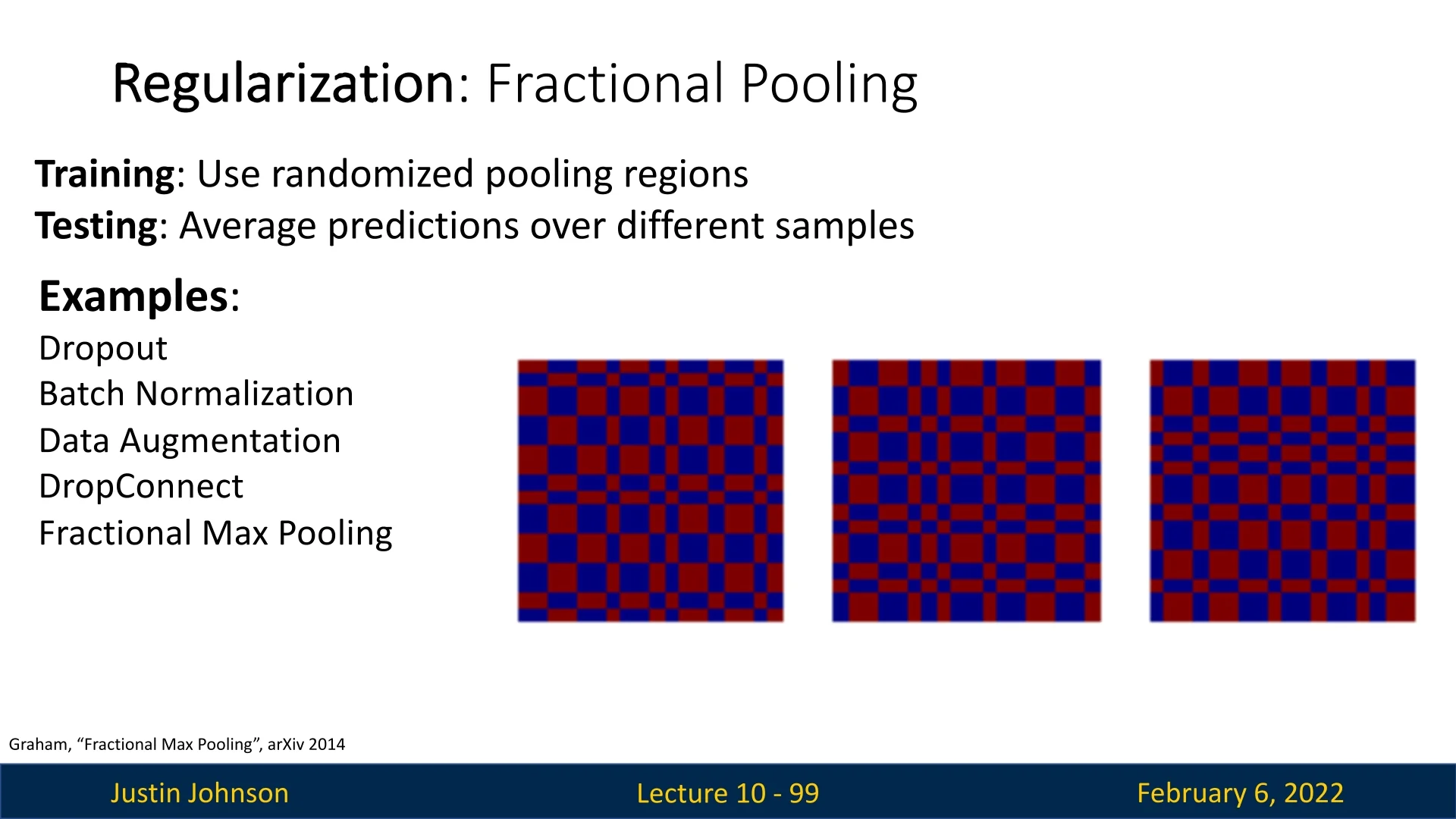
Effectiveness and Test-Time Strategy:
- This technique increases robustness to slight spatial distortions in input images by introducing controlled randomness in pooling.
- At test time, instead of using randomized pooling, we take the average of multiple forward passes to remove randomness while preserving the learned representations.
Stochastic Depth
Stochastic Depth [252] is a regularization technique designed for very deep networks, such as ResNets with hundreds of layers. Instead of using all layers during every forward pass, it randomly skips certain layers during training.
Why is this useful?
- It prevents deep networks from overfitting by creating an implicit ensemble of models.
- It allows gradients to flow more easily during backpropagation, reducing the vanishing gradient problem in extremely deep networks.
During training, each residual block is kept active with probability \( p_l \), meaning that the network effectively learns multiple sub-networks. At test time, all blocks are used, but each block’s contribution is scaled by its probability of survival \( p_l \), ensuring consistent behavior across training and inference.
The forward pass update rule for stochastic depth is:
\begin {equation} H^{\mbox{test}}_l = \mbox{ReLU}(p_l f(H^{\mbox{test}}_{l-1}; W_l) + H^{\mbox{test}}_{l-1}). \end {equation}
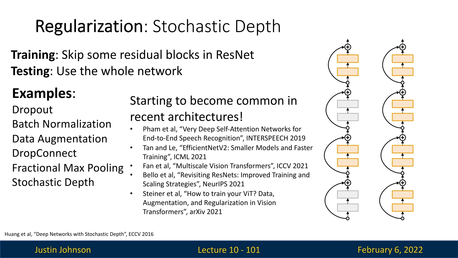
CutOut
CutOut [122] is a data augmentation technique that removes contiguous sections of input images. Unlike dropout, which randomly removes activations in intermediate layers, CutOut modifies the input space directly by masking out regions.
- It forces the network to learn robust representations by making it focus on the remaining visible parts of the image.
- This improves generalization, especially for small datasets, by preventing reliance on specific visual features.
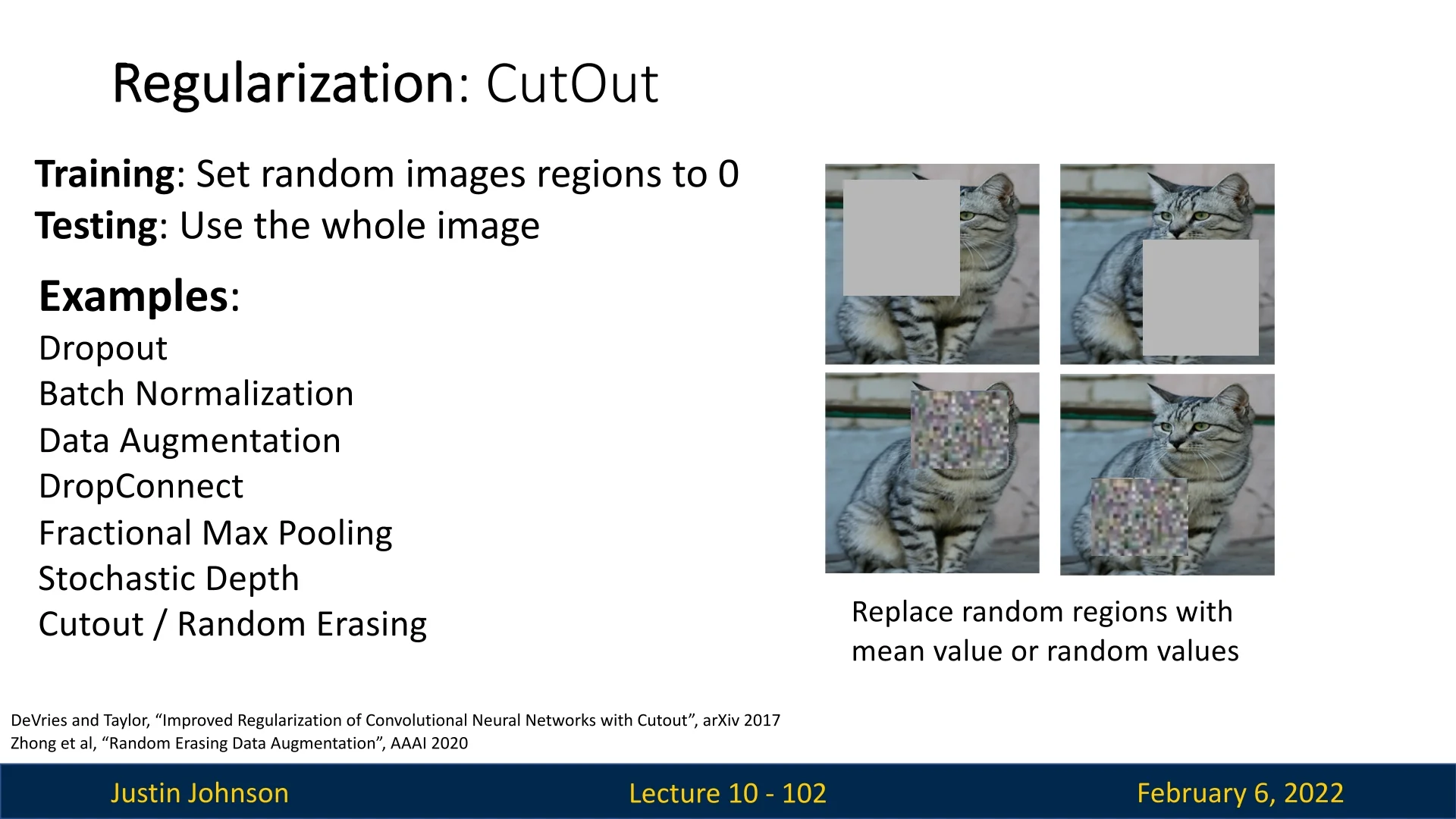
CutOut is closely related to denoising autoencoders and context encoders, as it forces the network to understand images in a global rather than local sense.
MixUp
MixUp [791] is a technique that improves generalization by training a network on convex combinations of input images and their labels.
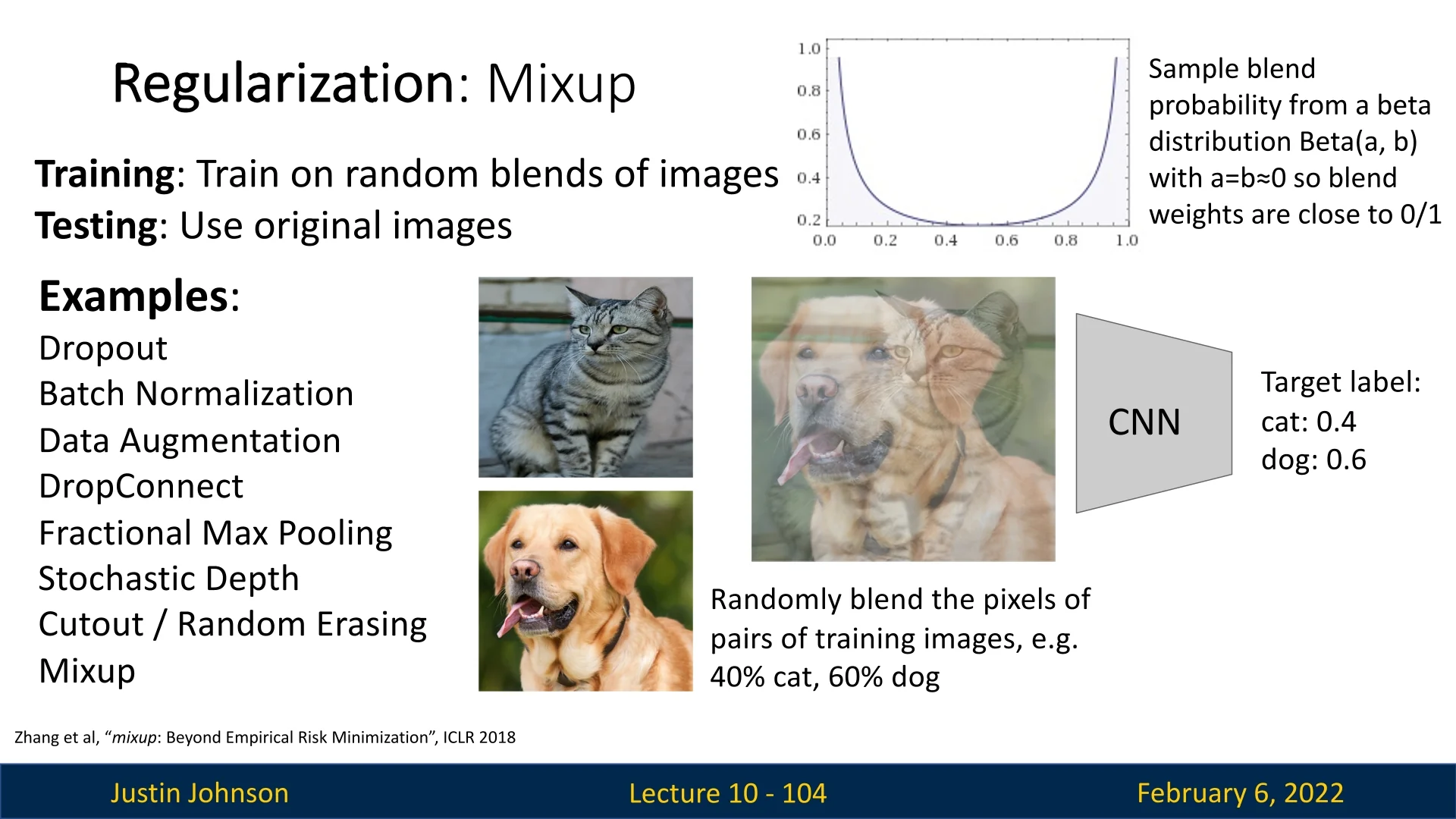
Instead of feeding original training samples, the model is trained with blended inputs:
\begin {equation} x' = \lambda x_i + (1 - \lambda ) x_j, \end {equation}
\begin {equation} y' = \lambda y_i + (1 - \lambda ) y_j. \end {equation}
where \( \lambda \) is drawn from a Beta distribution \( \mbox{Beta}(a, b) \). Usually \(a=b\approx 0\), making the weights close to 0/1 (e.g., 0.9cat, 0.1dog). This improves the results of using this regularization technique, in comparison with normal distribution (we are less likely to encounter situations of 0.5cat, 0.5dog, which can make it too hard for the model to learn sometimes).
Why does MixUp work?
- Encourages linear behavior between samples, reducing sharp decision boundaries that can lead to overfitting.
- Forces the model to learn representations that interpolate well between classes.
- Particularly effective for small datasets, where augmenting the diversity of training samples significantly improves generalization.
Summary and Regularization Guidelines
To summarize, different regularization techniques are useful in different scenarios:
- Use dropout in fully connected layers of deep networks.
- Batch normalization and augmentations (e.g., flips, color jittering) are almost always useful if appropriate for the task.
- CutOut and MixUp are particularly effective for small datasets, improving generalization.
- Stochastic depth is valuable for extremely deep architectures, such as ResNets with over 100 layers.