Lecture 18: Vision Transformers
18.1 Bringing Transformers to Vision Tasks
The Transformer architecture, built upon the foundation of self-attention, has revolutionized natural language processing by enabling models to capture long-range dependencies and contextual relationships in sequences. Given this success, researchers have sought to adapt self-attention mechanisms to computer vision tasks. However, unlike text, images are structured as two-dimensional grids with spatially correlated features, presenting unique challenges in directly applying self-attention.
This chapter explores how self-attention has been progressively integrated into vision models, beginning with augmenting traditional convolutional neural networks (CNNs) and ultimately evolving into fully attention-driven architectures. The goal is to understand how self-attention has transformed vision modeling—from enhancing existing CNNs to fully replacing convolutions with transformer-based structures.
We will explore three key approaches that highlight this progression:
- 1.
- Adding Self-Attention Layers to Existing CNN Architectures: The initial step involves integrating self-attention into standard CNN backbones (e.g., ResNet). This hybrid approach aims to enhance long-range dependency modeling within convolutional frameworks while preserving the spatial locality and efficiency of convolutions.
- 2.
- Replacing Convolution with Local Self-Attention Mechanisms: Moving beyond hybrid models, this approach eliminates convolutions by replacing them with local self-attention operations. While still constrained by locality, these models offer more flexible and dynamic feature aggregation than fixed convolution kernels.
- 3.
- Eliminating Convolutions Entirely with Fully Attention-Based Models: The final stage is the development of pure transformer architectures for vision, such as Vision Transformers (ViT) and their efficient variants. These models discard convolutions entirely, leveraging global self-attention to capture long-range relationships while benefiting from high parallelism and scalability.
Each approach builds upon the limitations of the previous, progressively leveraging the strengths of self-attention to overcome the constraints of convolutional architectures.
We begin by exploring the first approach: how self-attention layers were initially introduced into existing CNN frameworks to enhance their representational capacity.
18.2 Integrating Attention into Convolutional Neural Networks (CNNs)
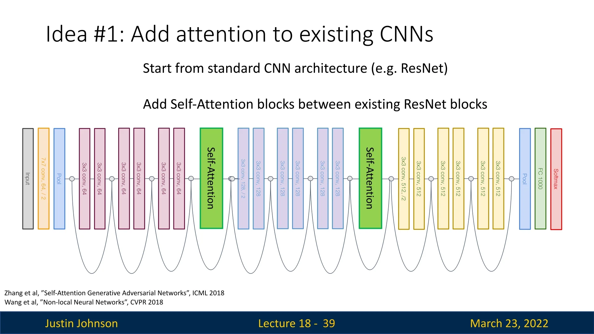
One of the earliest attempts to bring attention mechanisms into computer vision involved inserting self-attention layers into standard convolutional architectures such as ResNet. The idea is simple: take a well-established CNN and enhance it with attention layers at strategic points to improve its ability to model long-range dependencies.
This approach was explored in works such as:
- Self-Attention Generative Adversarial Networks (SAGAN) [784], which used self-attention in GANs to improve the quality of generated images.
- Non-Local Neural Networks [697], which introduced non-local operations that enable each pixel to aggregate information from distant regions in the image.
18.2.1 How Does It Work?
In these architectures, self-attention layers are inserted between standard convolutional blocks. These layers allow the network to selectively focus on relevant regions of the image, improving its ability to model long-range dependencies that are difficult for local convolutions (as it relies on limited receptive fields throughout most of the model).
18.2.2 Limitations of Adding Attention to CNNs
While augmenting CNNs with attention mechanisms enhances their ability to capture global context, it comes with several drawbacks:
- Increased Computational Cost: Adding attention layers increases the number of parameters and computation compared to standard CNNs. The pairwise attention computation scales quadratically with the number of pixels, making it inefficient for high-resolution images.
- Limited Parallelization: Convolution operations benefit from highly optimized implementations on modern hardware. Mixing convolutions with self-attention introduces irregular computations, reducing efficiency compared to fully convolutional models.
- Still Convolution-Dependent: Despite improvements, these models still rely on convolutions as their primary feature extractors. Attention enhances representations, but the model does not fully leverage the advantages of self-attention likes Transformers do in the use-case of sequence modeling.
To address these challenges, researchers explored an alternative approach: replacing convolutions with local self-attention mechanisms, aiming to enhance flexibility and dynamic feature aggregation while offering an efficiency improvement in comparison with the first idea (full self-attention layers throughout existing CNN architectures).
18.3 Replacing Convolution with Local Attention Mechanisms
Traditional convolutional layers in vision models apply fixed, learned kernels to aggregate local information across spatial locations. This approach is highly effective and hardware-efficient for capturing local patterns, but the aggregation weights are static at inference time: once training is complete, the same learned filter template is applied everywhere, regardless of the specific content within each local neighborhood.
Local self-attention offers a dynamic alternative [521]. Instead of applying a fixed kernel, the model computes data-dependent aggregation weights within a local window, allowing each spatial position to selectively emphasize the most relevant nearby features. This section introduces the mechanism, clarifies the representational trade-offs relative to convolution, and explains why local attention served as a stepping stone toward global attention in Vision Transformers.
18.3.1 Mechanism of Local Self-Attention
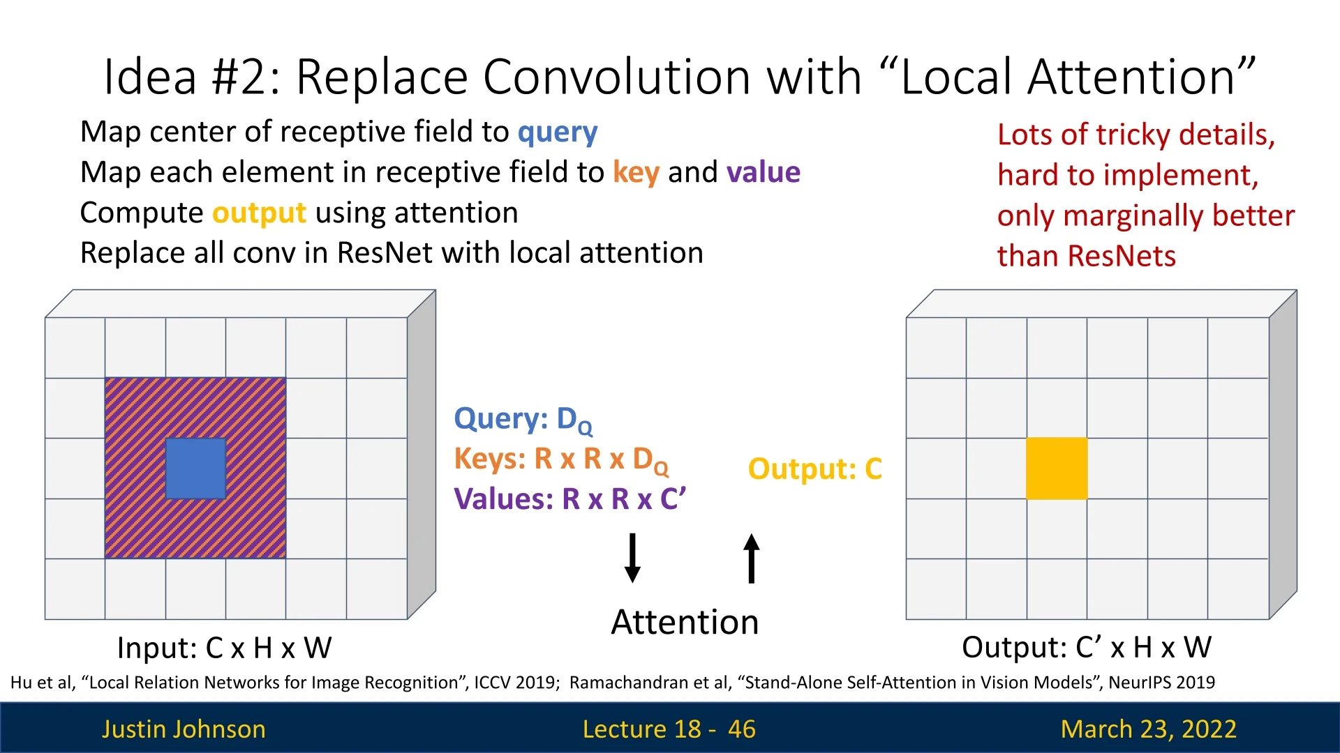
Local attention applies the standard query–key–value mechanism within a restricted spatial neighborhood. Consider an input feature map of shape \(C \times H \times W\). For each spatial location \((h,w)\), we define a \(K \times K\) window centered at \((h,w)\). The attention computation follows three steps:
- 1.
- Projection. The center feature vector is linearly projected to form a query \(q_{h,w} \in \mathbb {R}^{D}\). All vectors in the \(K \times K\) neighborhood are projected to keys \(k_{h',w'} \in \mathbb {R}^{D}\) and values \(v_{h',w'} \in \mathbb {R}^{C'}\), where \((h',w')\) ranges over the local window.
- 2.
- Local similarity scoring. The model computes dot-product similarities between the query and each local key: \[ \alpha _{(h,w)\rightarrow (h',w')} = \mbox{softmax}\!\left ( \frac {q_{h,w}^\top k_{h',w'}}{\sqrt {D}} \right ), \] where the softmax is taken over the \(K^2\) neighbors in the window.
- 3.
- Content-dependent aggregation. The output at \((h,w)\) is the weighted sum of local values: \[ y_{h,w} = \sum _{(h',w') \in \mathcal {N}_{K}(h,w)} \alpha _{(h,w)\rightarrow (h',w')} \, v_{h',w'}. \]
The resulting output feature map has shape \(C' \times H \times W\). The critical distinction from convolution is that the aggregation weights \(\alpha \) are computed from the input features themselves for each location, rather than being fixed parameters shared across all locations.
18.3.2 Why Local Attention Can Be More Adaptive than Convolution
Local self-attention and convolution both operate on sliding windows, but they differ in how they choose which information within the window matters most.
- Dynamic vs. fixed aggregation. A convolutional layer applies the same learned weighting pattern to every spatial window. Local attention computes a distinct weighting pattern for each query position. In a portrait, for example, local attention can assign higher weight to nearby edge-like features that define the jawline while down-weighting homogeneous skin regions, depending on the local content.
- Selective emphasis within the same window size. Even when the receptive field size \(K \times K\) matches a convolutional kernel, local attention can treat different neighbors as more or less relevant based on query–key similarity. This gives the model a principled way to suppress locally irrelevant structure without requiring a different kernel for each context.
These advantages are primarily representational. Whether they translate into practical gains depends on the task, model scale, and implementation efficiency, as discussed next.
18.3.3 Computational Considerations
Although convolution and local attention are both local-window operators, their cost profiles differ due to parameter sharing and memory access patterns.
Convolutional complexity A standard 2D convolution with kernel size \(K \times K\), input channels \(C_{\mbox{in}}\), and output channels \(C_{\mbox{out}}\) applied over a feature map of size \(H \times W\) has complexity: \begin {equation} \mathcal {O}\!\left ( H W \cdot C_{\mbox{in}} C_{\mbox{out}} \cdot K^2 \right ). \label {eq:chapter18_conv_complexity} \end {equation} The key efficiency driver is weight sharing: the same kernel parameters are reused across all \(HW\) locations. This regular computation pattern is also heavily accelerated in modern libraries and hardware.
Local attention complexity Local self-attention treats each location as a query token of dimension \(D\) and attends to \(K^2\) neighbors: \begin {equation} \mathcal {O}\!\left ( H W \cdot D \cdot K^2 \right ). \label {eq:chapter18_local_attn_complexity} \end {equation} The dominant operations are the local dot products for attention scores and the weighted aggregation of values.
Why local attention can be slower in practice Even when the asymptotic arithmetic looks comparable under rough dimension matching, local attention often incurs higher latency:
- Position-specific weights. Attention weights are computed uniquely for each location, reducing opportunities for reuse.
- Less regular memory access. Implementations must gather features from local neighborhoods to form keys and values. These gather-style operations are typically less cache-friendly than the contiguous access patterns of convolution.
18.3.4 From Local Attention to Vision Transformers
Empirical results in early studies indicated that local self-attention could match or slightly improve on comparable convolutional baselines on standard benchmarks, but the gains were often modest relative to the added implementation complexity and runtime overhead [521].
More importantly, restricting attention to local windows retains a fundamental limitation shared with convolution: long-range dependencies emerge only after stacking many layers. This motivated the next step in the design trajectory. Rather than replacing convolution with a different local operator, the Vision Transformer family replaces the local sliding-window paradigm with global self-attention over image tokens. By processing patch embeddings as a sequence and applying standard Transformer blocks globally, ViTs allow long-range interactions from the earliest layers, setting the stage for the architectural shift explored in the next sections.
18.4 Vision Transformers (ViTs): From Pixels to Patches
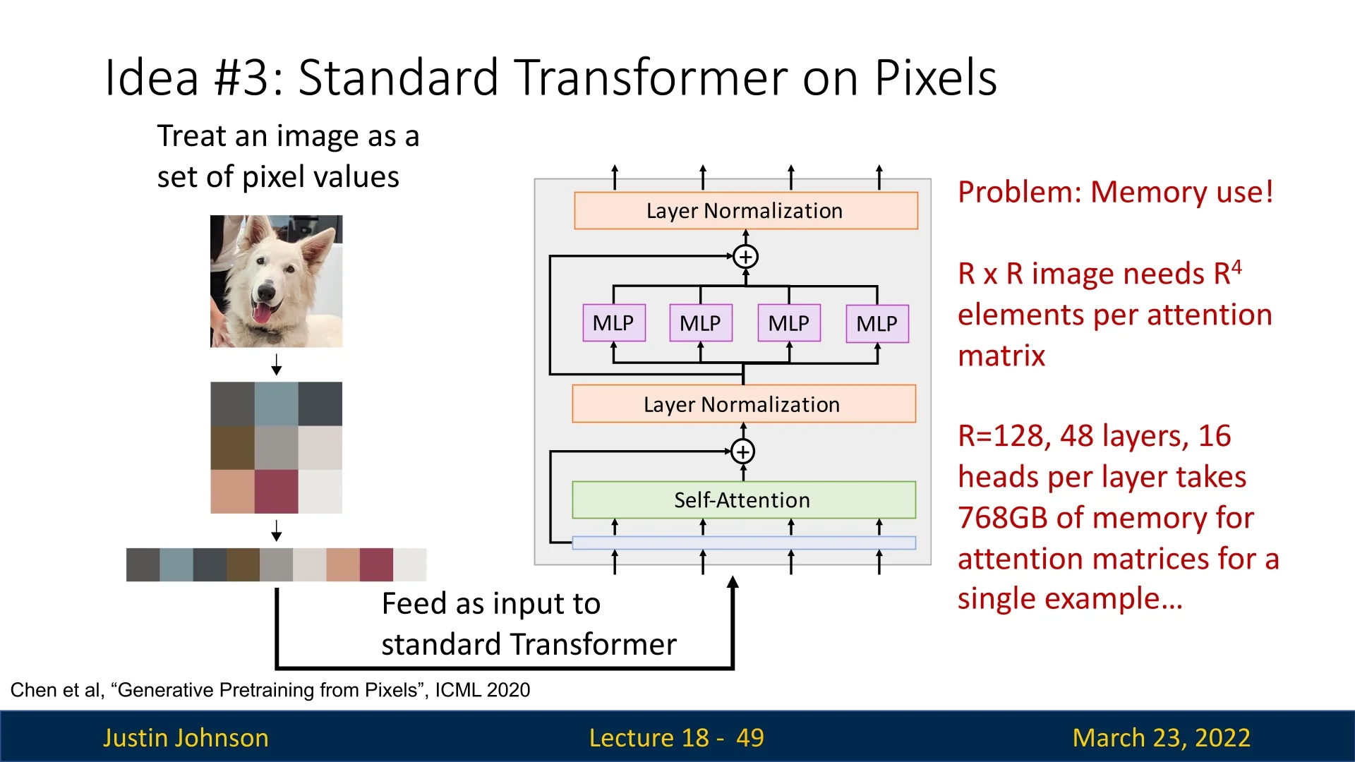
While global self-attention in ViTs enables long-range dependency modeling, applying standard transformers directly to image pixels presents a severe memory bottleneck. This approach, explored in [84], suffers from quadratic complexity with respect to image size. Specifically, for an \( R \times R \) image, the self-attention mechanism requires storing and computing attention weights for \( O(R^4) \) elements, making it impractical for high-resolution images. For instance, an image with \( R = 128 \), using 48 transformer layers and 16 heads per layer, requires an estimated 768GB of memory just for attention matrices—far exceeding typical hardware capacities.
To address this, Vision Transformers (ViT) [134] proposed a novel idea: processing images as patches instead of raw pixels. This drastically reduces the number of tokens, making global self-attention computationally feasible.
18.4.1 Splitting an Image into Patches
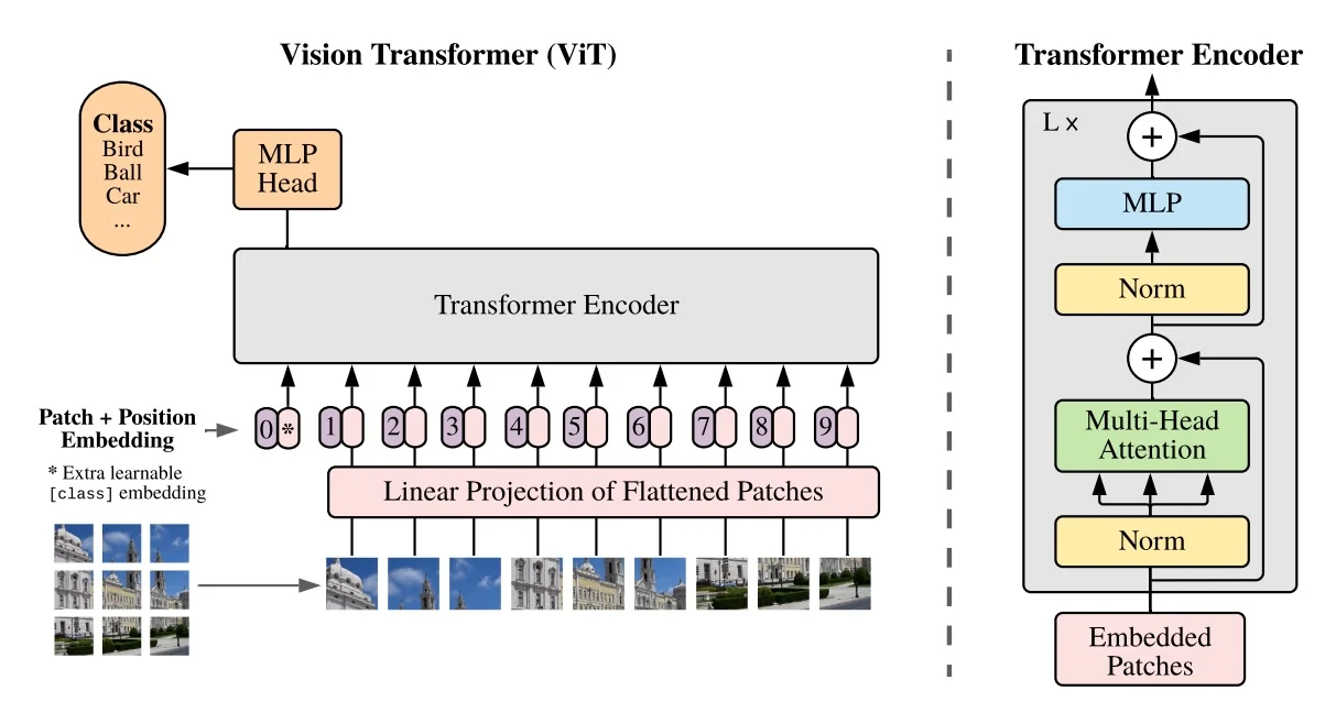
The Vision Transformer (ViT) applies the standard Transformer encoder to images with minimal modifications. Instead of processing raw pixels, it treats images as sequences of fixed-size patches, significantly reducing computational complexity compared to pixel-level attention.
To transform an image into a sequence of patches:
- 1.
- The image is divided into non-overlapping patches of size \( P \times P \).
- 2.
- Each patch, originally of shape \( P \times P \times C \), is flattened into a vector of size \( P^2C \).
- 3.
- A linear projection layer maps this vector into a \( D \)-dimensional embedding: \begin {equation} \mathbf {z}_i = W \cdot \mbox{Flatten}(\mathbf {x}_i) + b, \quad \mathbf {z}_i \in \mathbb {R}^D. \end {equation}
This transformation is essential because:
- It allows the model to learn how to encode image patches into a meaningful, high-level representation.
- Unlike raw pixel values, the learned embedding provides a semantic abstraction, grouping visually similar patches closer together.
- It reduces redundancy by filtering out unimportant pixel-level noise before processing by the Transformer.
The input image can be patched using a convolutional layer by setting the stride equal to the patch size. This ensures the image is partitioned into non-overlapping patches that are then flattened and processed as tokens.
18.4.2 Class Token and Positional Encoding
ViT introduces a learnable classification token ([CLS]), similar to BERT, to aggregate global image information. This token is prepended to the sequence of patch embeddings and participates in self-attention, enabling it to encode high-level features from all patches. The self-attention mechanism allows [CLS] to attend to all tokens, condensing the sequence into a fixed-size representation optimal for classification or regression.
- The [CLS] token acts as an information sink, gathering contextual features across all patches.
- It ensures a consistent, fixed-size output regardless of the input length.
- Unlike selecting an arbitrary patch for classification, using [CLS] avoids position-related biases and stabilizes training.
- Since [CLS] is trainable, it progressively refines its representation over multiple attention layers.
Additionally, since self-attention is permutation equivariant (i.e., it treats input elements as an unordered set), positional embeddings are added to the patch embeddings to preserve spatial order.
For a \( 224 \times 224 \times C \) image (where \( C \) is the number of channels), dividing it into \( 16 \times 16 \) patches: \begin {equation} N = \frac {224}{16} \times \frac {224}{16} = 14 \times 14 = 196. \end {equation}
Each patch is then flattened and projected into an embedding space before being processed by the Transformer.
18.4.3 Final Processing: From Context Token to Classification
Once the image patches and class token have been processed through the transformer encoder, we obtain the final encoded representation \( C \). The output of the encoder consists of the processed patch embeddings, along with the updated class token embedding \( c_0 \). This class token serves, as we mentioned, as a context vector that aggregates information from all patches through self-attention.
For classification tasks, we are only interested in the class token \( c_0 \), which is passed through a final MLP head to produce the output prediction (e.g., in the case of classification, the final probability vector is computed using a softmax layer).
18.4.4 Vision Transformer: Process Summary and Implementation
Vision Transformer Processing Steps
- 1.
- Image Patch Tokenization: Divide the input image into non-overlapping patches of size \(P \times P\). Each patch is flattened into a vector of size \(P^2 \, C\), where \(C\) is the number of channels.
- 2.
- Linear Projection of Patches: Map each flattened patch into a high-dimensional embedding space of dimension \(D\). This “patch embedding” transforms raw pixels into meaningful feature vectors.
- 3.
- Appending the Class Token: Prepend a learnable [CLS] token to the sequence of patch embeddings. This token will aggregate global context after the Transformer encoder.
- 4.
- Adding Positional Embeddings: Since self-attention alone lacks spatial awareness, add learned positional embeddings to each token to preserve patch-order information.
- 5.
- Transformer Encoder: Pass the token sequence through multiple stacked
Transformer blocks, each containing:
- Multi-Head Self-Attention: Allows patches to share information across the entire sequence.
- Feed-Forward Network (FFN): Enriches each token’s representation independently.
- Residual Connections and Layer Normalization: Stabilize training and improve gradient flow.
- 6.
- Class Token Representation: After processing, the [CLS] token encodes a global summary of the image.
- 7.
- Final Classification via MLP Head: Feed the final [CLS] representation into a small MLP head to obtain classification outputs (e.g., class probabilities).
PyTorch Implementation of a Vision Transformer
Below is an illustrative PyTorch example that shows how an image is divided into patches, passed through stacked Transformer blocks, and finally classified. Each portion of the code is explained to clarify the rationale behind the patching process, positional embeddings, Transformer blocks, and [CLS] token usage.
class VisionTransformer(nn.Module):
    """
    Inspired by:
    - https://github.com/lucidrains/vit-pytorch
    - https://github.com/jeonsworld/ViT-pytorch

    Args:
    image_size: (int) input image height/width (assuming square).
    patch_size: (int) patch height/width (assuming square).
    in_channels: (int) number of channels in the input image.
    hidden_dim: (int) dimension of token embeddings.
    num_heads: (int) number of attention heads in each block.
    num_layers: (int) how many Transformer blocks to stack.
    num_classes: (int) dimension of final classification output.
    mlp_ratio: (float) factor by which hidden_dim is expanded in the MLP.
    dropout: (float) dropout rate.
    """

    def __init__(
    self,
    image_size: int = 224,
    patch_size: int = 16,
    in_channels: int = 3,
    hidden_dim: int = 768,
    num_heads: int = 12,
    num_layers: int = 12,
    num_classes: int = 1000,
    mlp_ratio: float = 4.0,
    dropout: float = 0.0
    ):
        super().__init__()

        assert image_size % patch_size == 0, "Image dimensions must be divisible by the patch size."

        self.image_size = image_size
        self.patch_size = patch_size
        self.in_channels = in_channels
        self.hidden_dim = hidden_dim
        self.num_heads = num_heads
        self.num_layers = num_layers
        self.num_classes = num_classes

        # ----------------------------------------------------
        # 1) Patch Embedding
        # ----------------------------------------------------
        # Flatten each patch into patch_dim = (patch_size^2 * in_channels).
        # Then project to hidden_dim.
        patch_dim = patch_size * patch_size * in_channels
        self.num_patches = (image_size // patch_size) * (image_size // patch_size)

        self.patch_embed = nn.Linear(patch_dim, hidden_dim)

        # ----------------------------------------------------
        # 2) Learnable [CLS] token
        # ----------------------------------------------------
        # shape: (1, 1, hidden_dim)
        self.cls_token = nn.Parameter(torch.zeros(1, 1, hidden_dim))

        # ----------------------------------------------------
        # 3) Positional Embeddings
        # ----------------------------------------------------
        # shape: (1, num_patches + 1, hidden_dim)
        # +1 for the [CLS] token.
        self.pos_embedding = nn.Parameter(torch.zeros(1, self.num_patches + 1, hidden_dim))

        # ----------------------------------------------------
        # 4) Dropout (Optional)
        # ----------------------------------------------------
        self.pos_drop = nn.Dropout(dropout)

        # ----------------------------------------------------
        # 5) Transformer Blocks
        # ----------------------------------------------------
        self.blocks = nn.ModuleList([
        TransformerBlock(embed_dim=hidden_dim,
        num_heads=num_heads,
        mlp_ratio=mlp_ratio,
        dropout=dropout)
        for _ in range(num_layers)
        ])

        # ----------------------------------------------------
        # 6) Final LayerNorm and Classification Head
        # ----------------------------------------------------
        self.norm = nn.LayerNorm(hidden_dim)
        self.head = nn.Linear(hidden_dim, num_classes)

        # Optionally initialize weights here
        self._init_weights()

    def _init_weights(self):
        """
        A simple weight initialization scheme.
        """
        for m in self.modules():
            if isinstance(m, nn.Linear):
                nn.init.xavier_uniform_(m.weight)
            if m.bias is not None:
                nn.init.zeros_(m.bias)
            elif isinstance(m, nn.LayerNorm):
                nn.init.ones_(m.weight)
                nn.init.zeros_(m.bias)

    def forward(self, x):
        """
        Forward pass:
        x: shape (B, C, H, W) with:
        B = batch size
        C = in_channels
        H = W = image_size
        """
        B = x.shape[0]

        # ----------------------------------------------------
        # (A) Create patches: (B, num_patches, patch_dim)
        # ----------------------------------------------------
        # Flatten patches: each patch is patch_size x patch_size x in_channels
        # We’ll use simple .view or rearranging. Below uses .unfold (similar).
        # For clarity, here’s a naive approach with reshape:

        # 1) Flatten entire image: (B, C, H*W)
        # 2) Reshape to group patches: (B, num_patches, patch_dim)
        #    patch_dim = patch_size^2 * in_channels
        # This works if patch_size divides H and W exactly
        # but requires reordering in row-major patch order.

        # A simpler approach is:
        patches = x.unfold(2, self.patch_size, self.patch_size)\
        .unfold(3, self.patch_size, self.patch_size)  # (B, C, nH, nW, pH, pW)
        # nH = H / patch_size, nW = W / patch_size
        patches = patches.permute(0, 2, 3, 1, 4, 5)                # (B, nH, nW, C, pH, pW)
        patches = patches.reshape(B, self.num_patches, -1)         # (B, num_patches, patch_dim)

        # ----------------------------------------------------
        # (B) Patch Embedding
        # ----------------------------------------------------
        tokens = self.patch_embed(patches)  # (B, num_patches, hidden_dim)

        # ----------------------------------------------------
        # (C) Add the [CLS] token
        # ----------------------------------------------------
        cls_tokens = self.cls_token.expand(B, -1, -1)  # (B, 1, hidden_dim)
        tokens = torch.cat([cls_tokens, tokens], dim=1)  # (B, num_patches+1, hidden_dim)

        # ----------------------------------------------------
        # (D) Add learnable positional embeddings
        # ----------------------------------------------------
        tokens = tokens + self.pos_embedding[:, : tokens.size(1), :]
        tokens = self.pos_drop(tokens)

        # ----------------------------------------------------
        # (E) Pass through Transformer Blocks
        # ----------------------------------------------------
        for blk in self.blocks:
            tokens = blk(tokens)

        # ----------------------------------------------------
        # (F) LayerNorm -> Classification Head
        # ----------------------------------------------------
        cls_final = self.norm(tokens[:, 0])  # the [CLS] token output
        logits = self.head(cls_final)       # (B, num_classes)

        return logits

# --------------------------------------------------------
#  Example Usage
# --------------------------------------------------------
if __name__ == "__main__":
    # Suppose we have a batch of 8 images, each 3 x 224 x 224
    model = VisionTransformer(image_size=224,
    patch_size=16,
    in_channels=3,
    hidden_dim=768,
    num_heads=12,
    num_layers=12,
    num_classes=1000)
    dummy_images = torch.randn(8, 3, 224, 224)
    out = model(dummy_images)  # (8, 1000)
    print("Output shape:", out.shape)
Applying self-attention at the pixel level is computationally prohibitive, requiring each pixel to interact with every other pixel, resulting in an infeasible \( O(R^4) \) complexity for high-resolution images. To address this, Vision Transformers (ViT) process images as sequences of patches rather than individual pixels.
By dividing an image into fixed-size patches, ViT significantly reduces the number of tokens in self-attention while preserving global context. This enables efficient long-range dependency modeling across semantically meaningful regions with lower memory overhead.
To illustrate this advantage, we now compare the computational complexity of pixel-level self-attention versus patch-based self-attention in ViT.
18.4.5 Computational Complexity: ViT vs. Pixel-Level Self-Attention
A core challenge in applying Transformers to images is the quadratic nature of self-attention in the number of tokens. Below, we compare two approaches: directly treating every pixel as a separate token (pixel-level self-attention), versus splitting the image into larger patches (as in the Vision Transformer, ViT).
Pixel-Level Self-Attention
- An image of size \(R \times R\) contains \(R^2\) pixels.
- Self-attention compares each token (pixel) to every other token, incurring a complexity of \[ O\bigl (\underbrace {R^2}_{\mbox{tokens}} \times \underbrace {R^2}_{\mbox{all-pairs}}\bigr ) \;=\; O(R^4). \]
- As an example, for \(128 \times 128\) images with many layers and heads, Chen et al. [84] report memory usage in the hundreds of gigabytes just to store attention matrices, highlighting how quickly \(R^4\) becomes infeasible.
Patch-Based Self-Attention (ViT)
- Instead of using all \(R^2\) pixels as tokens, ViT groups the image into \(N\) non-overlapping patches, each of size \(P \times P\).
- The total number of patches is \[ N \;=\; \left (\frac {R}{P}\right )^2, \] so the self-attention complexity becomes \[ O(N^2) \;=\; O\!\Bigl (\bigl (\tfrac {R^2}{P^2}\bigr )^2\Bigr ) \;=\; O\!\Bigl (\frac {R^4}{P^4}\Bigr ). \]
- Example: \[ R = 224,\quad P = 16 \;\;\Longrightarrow \;\; R^2 = 50{,}176\;\;\mbox{(tokens if using pixels)}, \quad N = \bigl (\tfrac {224}{16}\bigr )^2 = 196. \] Thus, we reduce the token count from \(50{,}176\) to \(196\), which is a 256-fold reduction in the number of tokens. In terms of all-pairs interactions, that is a \(\,256^2\!=\!65{,}536\)-fold reduction in total attention computations.
Key Takeaways
- Pixel-level self-attention has \(O(R^4)\) complexity and quickly becomes intractable for even moderately large images.
- Patch-based self-attention (ViT) cuts down the number of tokens to \(N = (R/P)^2\), reducing complexity to \(O(N^2)\!=\!O\bigl (R^4/P^4\bigr )\). Even a modest patch size \(P\) massively lowers the computational and memory burden.
- Grouping pixels into patches retains the Transformer’s ability to capture global interactions among tokens but at a fraction of the cost compared to pixel-level processing.
Hence, ViT avoids the prohibitive \(R^4\) scaling of naive pixel-level self-attention, making Transformers viable for high-resolution imagery on modern hardware.
This shift to patch-based processing laid the foundation for scalable Vision Transformers, making them practical for real-world applications.
18.4.6 Limitations and Data Requirements of Vision Transformers
While Vision Transformers (ViTs) [134] have demonstrated state-of-the-art performance in many vision tasks, their training requirements differ significantly from Convolutional Neural Networks (CNNs). Specifically, ViTs are often described as being more data hungry, requiring much larger datasets to outperform CNNs. This section examines the factors contributing to this behavior and explores strategies to improve ViT training efficiency.
Large-Scale Pretraining is Critical
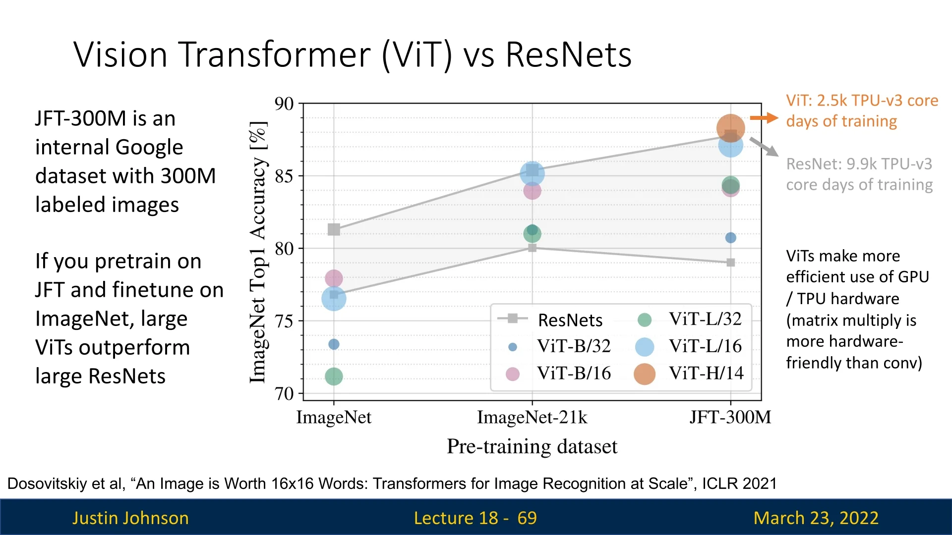
ViTs lack the spatial priors present in CNNs, such as locality and translation equivariance, which help CNNs generalize well from relatively small datasets. This difference becomes evident when comparing training performance: the ViT paper [134] found that ViTs trained from scratch on ImageNet (1.3M images) underperform compared to similarly sized ResNet models. However, when pre-trained on much larger datasets—such as ImageNet-21k (14M images, over 10× larger) or JFT-300M (300M images, over 200× larger)—ViTs surpass CNNs in accuracy. These findings suggest that ViTs require far more data to match or exceed CNN performance. Large-scale pretraining helps compensate for this by providing enough data for the model to discover robust representations from scratch.
A comparison of ImageNet Top-1 accuracy between ViTs and CNNs reveals that ViTs trained solely on ImageNet tend to underperform large ResNets. However, as dataset size increases, ViTs gradually surpass CNNs. This suggests that ViTs require substantially more data to reach competitive performance levels.
Why Do ViTs Require More Data?
Vision Transformers (ViTs) often require more data than comparable convolutional neural networks (CNNs) to reach strong performance when trained from scratch. A practical way to summarize the gap is that CNNs hard-code several useful structural constraints for images, while standard ViTs expose a more flexible modeling space and therefore rely on data and training strategy to discover the same regularities. Below we outline the main architectural and optimization factors that have been observed to contribute to this data requirement.
1. Fewer hard-coded spatial constraints CNNs enforce local connectivity: each output feature depends on a small contiguous neighborhood. This matches the empirical fact that nearby pixels are often strongly correlated. Weight sharing further ensures that the same local pattern detector is reused across all spatial positions.
In contrast, a standard ViT represents an image as a sequence of patches and applies global self-attention. While this is highly expressive, it does not automatically privilege local neighborhoods. The model can learn locality, but it must infer this preference from examples rather than receiving it as a built-in constraint. This typically increases the amount of data needed to learn stable low-level visual regularities.
2. Weaker translation handling by design Convolution applies the same filter everywhere, so the detection of a feature is naturally consistent across spatial shifts. This property reduces the number of distinct training examples required to cover the same object appearing in many positions.
ViTs share the projection matrices used to form \(Q, K, V\), but the attention patterns themselves are content-dependent and rely on positional information to represent spatial structure. As a result, the model may need more varied examples to become as robust to spatial variation as a CNN with a similar parameter budget.
3. Isotropic token processing versus explicit multi-scale pipelines Standard CNN backbones typically build a pyramidal hierarchy. Spatial resolution is reduced progressively (via pooling or strided convolutions) while feature abstraction increases. This provides a strong, stage-wise path from local edges and textures to parts and objects.
The original ViT is isotropic: it maintains a fixed token grid and a constant embedding dimension across depth. The model can learn hierarchical organization implicitly, but it is not guided by an explicit multi-scale schedule. This enlarges the space of plausible solutions, which again can increase data requirements. Later architectures that reintroduce structured locality or hierarchy (for example, windowed or multi-stage designs) can mitigate this behavior.
4. Greater dependence on explicit regularization and augmentation Because standard ViTs allow global interactions from the first layer, they often benefit substantially from strong training-time controls when data is limited. In practice, competitive ViT training on ImageNet-scale datasets typically relies on:
- Strong data augmentation (e.g., Mixup, CutMix, RandAugment).
- Stochastic depth and dropout variants.
- Careful optimization and weight decay schedules.
These techniques help constrain fitting behavior that CNNs partially regulate through their fixed local structure and weight sharing patterns.
Summary The practical takeaway is not that ViTs are inherently inferior on smaller datasets, but that their default design places more responsibility on data scale and training strategy. With sufficient pretraining data or carefully tuned augmentation and regularization, ViTs can match or exceed CNNs. When data is scarce and training is from scratch, CNN-style structural constraints still offer a reliable advantage.
18.4.7 Understanding ViT Model Variants
Vision Transformers (ViTs) come in different sizes and configurations. Each model is typically named using the format ViT-Size/Patch, where:
-
Size indicates the model capacity:
- Ti (Tiny), S (Small), B (Base), L (Large), and H (Huge).
- Patch refers to the patch resolution, such as \(16 \times 16\), \(32 \times 32\), or \(14 \times 14\), written as /16, /32, or /14.
For example, ViT-B/16 represents the base variant with a patch size of \(16 \times 16\), and is one of the most commonly used ViT configurations.
Model Configurations
Smaller patch sizes lead to longer input sequences and higher compute, but often better accuracy due to more spatial detail. Larger models (e.g., ViT-L/16 or ViT-H/14) benefit from scale when trained on sufficiently large datasets.
Transfer Performance Across Datasets
The ViT paper [134] shows that model performance scales with both dataset size and compute. For example:
- ViT-B/16 reaches 84.2% top-1 accuracy on ImageNet when pretrained on JFT-300M.
- ViT-L/16 pushes this to 87.1% with more epochs.
- ViT-H/14 achieves up to 88.1% top-1 on ImageNet and 97.5% on Oxford-IIIT Pets.
In summary, the Vision Transformer (ViT) model naming convention captures both model size and patch granularity—factors that directly influence performance, memory usage, and training time. Larger models and smaller patches typically improve accuracy, but at a significantly higher computational cost.
However, one critical limitation still looms large: ViTs struggle when trained on modest-sized datasets. Unlike CNNs, which benefit from strong inductive biases like translation equivariance and locality, ViTs require extensive data to generalize well. For example, while CNNs achieve strong results on ImageNet (\(\sim 1.3\)M images), ViTs originally required datasets 30–300 times larger to outperform them.
This raises a key question: Can we make ViTs more data-efficient and easier to train on standard-sized datasets? The following parts explore this challenge—starting with how targeted use of regularization and data augmentation can bridge the performance gap between ViTs and CNNs.
18.4.8 Improving ViT Training Efficiency
Given that ViTs require large-scale data to perform well, an important research question is: How can we make ViTs more efficient on smaller datasets? The work of Steiner et al. [611] demonstrated that regularization and data augmentation play a critical role in improving ViT training, reducing the gap between ViTs and CNNs on smaller datasets.
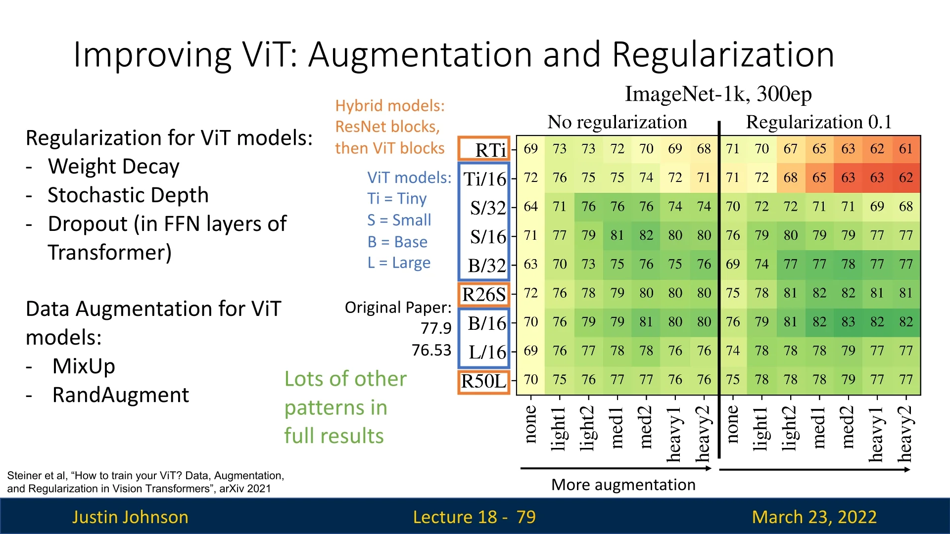
Regularization Techniques: The same regularization techniques discussed in (§18) are critical for stabilizing and improving ViT training. These techniques prevent overfitting, enhance generalization, and help ViTs converge more efficiently, even with limited training data.
- Weight Decay: Introduces an \(L_2\) penalty to the model parameters, discouraging large weights and improving generalization.
- Stochastic Depth: Randomly drops entire residual blocks during training, acting as an implicit ensemble method that reduces overfitting.
- Dropout in FFN Layers: Introduces stochasticity within the feed-forward network, preventing the model from relying too heavily on specific neurons.
Data Augmentation Strategies: As explored in [ref], data augmentation is a powerful tool for improving generalization by artificially expanding the training set with transformations that preserve class identity.
- MixUp: Blends two images and their labels, encouraging the model to learn smoother decision boundaries and avoid overconfidence.
- RandAugment: Applies a combination of randomized augmentations, exposing the model to diverse variations of the data.
Experimental results show that combining multiple forms of augmentation and regularization significantly improves ViT performance, especially on datasets like ImageNet. Figure 18.6 illustrates how adding more augmentation and regularization often improves ViT accuracy.
Towards Data-Efficient Vision Transformers: Introducing DeiT
While improving training strategies helps, a fundamental question remains: Can we design a ViT variant that is inherently more data-efficient? This question led to the development of Data-Efficient Image Transformers (DeiT) [647], which we will explore in the next section. DeiT introduces several key training improvements, allowing ViTs to match CNN performance even when trained on ImageNet-scale datasets without external pretraining.
18.5 Data-Efficient Image Transformers (DeiTs)
While Vision Transformers (ViTs) demonstrate strong performance on large-scale datasets such as ImageNet-21k or JFT-300M, their reliance on extensive pretraining limits accessibility in settings where only mid-scale labeled data are available. A canonical example is ImageNet-1k (\(\sim \)1.3M images), where early ViT training recipes lagged behind similarly sized CNNs unless supplemented with much larger external corpora.
To address this gap, Touvron et al. introduced the Data-Efficient Image Transformer (DeiT) [647]. The goal was to keep the core ViT design largely intact, while closing the ImageNet-1k performance gap through a transformer-specific training recipe and a lightweight distillation mechanism implemented inside the token sequence.
- DeiT models are trained on ImageNet-1k only, with no additional large-scale pretraining [647].
- The authors report training on a single 8-GPU node in roughly two to three days for the main models, with an optional high-resolution fine-tuning stage [647].
- With this recipe, DeiT matches or outperforms strong CNN baselines at comparable compute and parameter budgets on ImageNet-1k [647].
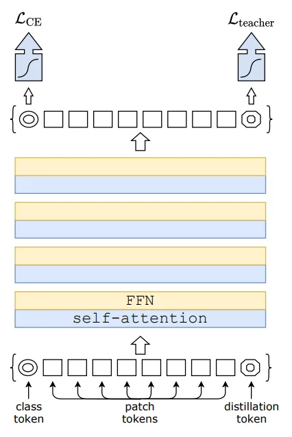
A central contribution is distillation through attention. DeiT introduces an additional learnable token, [DIST], which is trained to imitate the predictions of a strong CNN teacher. This enables a ViT student to benefit from the teacher’s mature supervision signal, while retaining the transformer architecture and avoiding extra inference-time cost beyond a second classification head.
Before presenting the distillation token mechanism, we briefly review the two losses that motivate the distinction between “hard” and “soft” distillation: cross-entropy and KL divergence.
18.5.1 Cross-Entropy and KL Divergence: Theory, Intuition, and Role in Distillation
Cross-Entropy Loss Cross-entropy (CE) is the standard objective for supervised classification. Given a predicted probability distribution \( \mathbf {p} = (p_1, \dots , p_n) \) and a one-hot target \( \mathbf {y} \), the loss is \begin {equation} \mathcal {L}_{\mbox{CE}}(\mathbf {y}, \mathbf {p}) = - \sum _{i} y_i \log p_i = -\log p_{\mbox{correct}}. \label {eq:chapter18_deit_ce} \end {equation}
Because CE depends only on the probability assigned to the correct class, it provides a strong but narrow supervision signal:
- It penalizes incorrect predictions in proportion to how small \(p_{\mbox{correct}}\) is.
- It does not distinguish between different ways of distributing probability mass among incorrect classes.
In practice, this means CE does not explicitly communicate whether the model confuses the correct class with a visually similar alternative or with an unrelated category.
KL Divergence: Full Distribution Matching Knowledge distillation often leverages the Kullback-Leibler divergence to match a full teacher distribution \(P\) with a student distribution \(Q\): \begin {equation} \mbox{KL}(P \| Q) = \sum _i P(i) \log \frac {P(i)}{Q(i)}. \label {eq:chapter18_deit_kl} \end {equation}
When used as a training signal, this objective encourages the student to reproduce the teacher’s relative preferences across classes, not merely the top-1 decision.
Illustrative Example: CE vs. KL Consider three classes cat, dog, rabbit. Suppose the teacher is unsure between cat and dog, outputting: \[ P = [0.50, 0.49, 0.01]. \] Now consider two students. Both predict the correct class (cat) with 50% probability, but distribute the remaining mass differently: \[ Q_1 = [0.50, 0.45, 0.05] \quad \mbox{(matches teacher structure)}, \] \[ Q_2 = [0.50, 0.01, 0.49] \quad \mbox{(matches top-1, but structurally wrong)}. \] Assuming cat is the ground truth, CE views both students as identical: \begin {align*} \text {CE}(Q_1) &= -\log 0.50 \approx 0.693, \\ \text {CE}(Q_2) &= -\log 0.50 \approx 0.693. \end {align*}
However, KL divergence reveals that \(Q_2\) has completely missed the teacher’s insight (that dog is the runner-up, not rabbit): \begin {align*} \text {KL}(P \| Q_1) &\approx 0.025 \quad \text {(very low)}, \\ \text {KL}(P \| Q_2) &\approx 1.862 \quad \text {(very high)}. \end {align*}
Thus, while CE treats both predictions as equally ”good” (based solely on the target class), KL imposes a heavy penalty on \(Q_2\) for failing to capture the semantic relationship between classes.
Hard vs. Soft Distillation Distillation can be implemented using either:
- Soft distillation, where the student matches the teacher’s soft probability distribution, typically via a temperature-scaled KL objective.
- Hard distillation, where the teacher’s top-1 prediction is converted into a hard label \(y_t\), and the student is trained with CE, similar to pseudo-labeling.
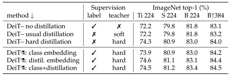
In DeiT, the authors report that hard distillation outperforms soft distillation on ImageNet-1k, especially when implemented through a dedicated distillation token [647]. This empirical result motivates the token-based design described next.
18.5.2 DeiT Distillation Token and Training Strategy
DeiT improves the data efficiency of Vision Transformers by embedding knowledge distillation inside the Transformer sequence. Concretely, the ViT input is extended by prepending two learnable tokens:
- [CLS]: supervised using the ground-truth label.
- [DIST]: supervised using a teacher model’s prediction.
Both tokens participate in all self-attention layers. This means the model does not merely receive a teacher signal at the final classifier; instead, the teacher-supervised summary token can shape intermediate representations through repeated interaction with patch tokens and with the [CLS] token.
Why a Dedicated Distillation Token?
A natural question is why DeiT needs a dedicated [DIST] token when a [CLS] token already exists. Why not (i) apply the distillation loss directly to [CLS], or (ii) add a second [CLS]-like token supervised by the ground-truth label?
The DeiT paper provides evidence that the dedicated token is not a cosmetic change but a functional separation of learning signals [647]:
- Avoiding objective interference. The ground-truth label and the teacher’s prediction can disagree on individual samples. Forcing a single token to satisfy both objectives can create conflicting gradients. Two tokens allow the model to maintain distinct summary streams for the human label and for the teacher’s decision, and to reconcile them only at the end.
- A second class token is empirically redundant. The authors explicitly tested a Transformer with two class tokens both trained with the same label objective. Even when initialized independently, the two class tokens rapidly converge to nearly identical representations (cosine similarity \(\sim 0.999\)) and provide no measurable performance gain [647]. This indicates that duplication without distinct supervision does not expand the useful hypothesis space.
- The distillation token learns complementary features. In contrast, the learned class and distillation tokens start far apart in representation space (average cosine similarity \(\sim 0.06\)), then gradually become more aligned through the network, reaching a high but not perfect similarity at the final layer (cosine \(\sim 0.93\)) [647]. This pattern is consistent with two non-identical objectives that are related but not the same.
At test time, DeiT can classify using either token head independently, but the best performance is obtained by late fusion of both heads, suggesting that the two summary embeddings encode complementary decision cues [647].
Hard Distillation: Counter-Intuitive but Effective
Standard knowledge distillation often emphasizes soft distribution matching, since a teacher’s full probability vector can encode fine-grained class relationships. DeiT reports a counter-intuitive result: for Transformers trained on ImageNet-1k, hard distillation (using only the teacher’s top-1 label) outperforms the soft KL-based alternative [647].
This holds even when distilling through only a class token, and becomes stronger with the dedicated distillation token and late fusion.
Let \(Z_{\mbox{cls}}\) and \(Z_{\mbox{dist}}\) denote the logits produced from the [CLS] and [DIST] tokens. With hard distillation, the training loss is: \begin {equation} \mathcal {L}_{\mbox{hard}} = \frac {1}{2}\mathcal {L}_{\mbox{CE}}(Z_{\mbox{cls}}, y) + \frac {1}{2}\mathcal {L}_{\mbox{CE}}(Z_{\mbox{dist}}, y_t), \label {eq:chapter18_deit_hard_distillation} \end {equation} where \(y\) is the ground-truth label and \(y_t = \arg \max _c Z_t(c)\) is the teacher’s top-1 label [647].
A plausible interpretation is that, in this data regime, the teacher’s single best decision provides a crisp auxiliary target that regularizes optimization, while avoiding sensitivity to teacher calibration differences across the long tail of classes. Empirically, the distillation embedding can even slightly outperform the class embedding when used alone, reinforcing the idea that the teacher-supervised token is not merely a redundant copy of [CLS] [647].
Overall, this design adds only a small second head and a single extra token, while providing a stable auxiliary supervision signal that complements the ground-truth objective.
Soft Distillation Objective
For completeness, the soft distillation variant uses a temperature-scaled KL term: \begin {equation} \mathcal {L}_{\mbox{soft}} = (1 - \lambda )\mathcal {L}_{\mbox{CE}}(Z_{\mbox{cls}}, y) + \lambda \tau ^2 \, \mbox{KL}\big (\psi (Z_{\mbox{dist}}/\tau ), \psi (Z_t/\tau )\big ), \label {eq:chapter18_deit_soft_distillation} \end {equation} where \(\psi \) is Softmax, \(\tau > 1\) flattens the distributions, and \(\lambda \in [0,1]\) balances the two terms [647].
Although this objective remains a principled way to transfer richer teacher uncertainty, DeiT’s evidence indicates that, for ImageNet-1k training of ViT-scale models, the simpler hard-label signal is the more effective choice when implemented through the dedicated distillation token and combined at inference by late fusion [647].
Why Use a CNN Teacher
DeiT distills from a strong CNN teacher, specifically RegNetY-16GF, which achieves high ImageNet accuracy at similar parameter scale [647]. Using a convolutional teacher is beneficial because it provides a complementary training signal shaped by years of mature CNN optimization and architectural refinement. In practice, this cross-family supervision appears to stabilize training and improve ImageNet-1k generalization for transformer students [647].
Learned Token Behavior
The [CLS] and [DIST] tokens evolve differently across depth. DeiT reports low similarity in early layers and substantially higher similarity near the output, indicating that the two tokens encode distinct intermediate information while converging toward consistent final predictions [647]. A control experiment adding a second unsupervised [CLS] token yields negligible gains, reinforcing that the benefit comes from the distinct teacher supervision rather than token redundancy.
Fine-Tuning at Higher Resolution
After training at \(224 \times 224\), DeiT optionally fine-tunes at higher resolution such as \(384 \times 384\) [647]. The patch size typically remains fixed, so increasing input resolution produces a finer-grained patch grid and a longer token sequence, rather than “higher-resolution patches”.
Positional Embedding Interpolation and Norm Preservation Because the token grid changes with resolution, the pretrained positional embeddings must be resized to match the new spatial layout. DeiT performs this resizing using bicubic interpolation and aims to approximately preserve the L2 norm of the positional embedding vectors to avoid magnitude shifts that would destabilize the pretrained transformer during fine-tuning [647].
Teacher Adaptation with FixRes When distillation is used during high-resolution fine-tuning, the teacher is evaluated on the same resolution regime. FixRes [645] provides a resolution-consistent evaluation and calibration procedure so the teacher remains effectively “frozen”, maintaining a reliable distillation signal at the new input size.
Consistency of the Distillation Signal DeiT maintains the same distillation paradigm during fine-tuning as in the base training stage [647]. When using hard distillation, the [DIST] token continues to be supervised by the teacher’s top-1 prediction, aligning the fine-tuning objective with the strategy that yielded the strongest ImageNet-1k results.
Why This Works in Data-Limited Settings
DeiT’s improved ImageNet-1k performance can be understood as the combination of two complementary ingredients:
- A strong transformer training recipe that narrows the gap between ViT and CNN baselines without external data.
- A token-level teacher signal that provides additional supervision beyond the ground-truth label, shaping intermediate representations through attention pathways [647].
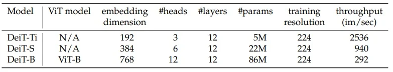
18.5.3 Model Variants
DeiT defines a small family of models that mirror ViT scaling patterns while keeping a fixed head dimension \(d=64\) [647]:
- DeiT-Ti: 192-dimensional embeddings, 3 attention heads.
- DeiT-S: 384-dimensional embeddings, 6 attention heads.
- DeiT-B: 768-dimensional embeddings, 12 attention heads (matching ViT-B).
18.5.4 Conclusion and Outlook: From DeiT to DeiT III and Beyond
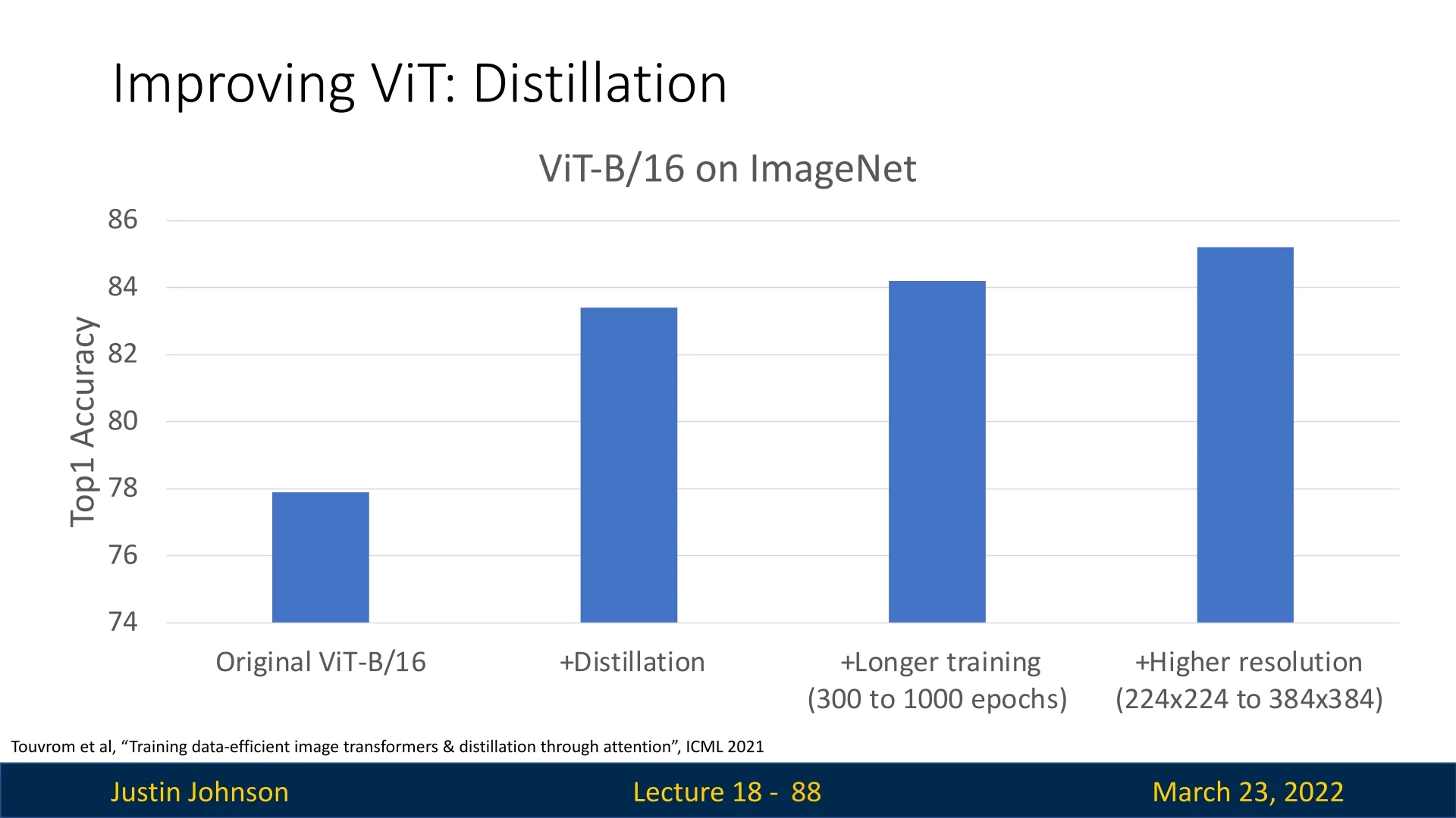
The Data-efficient Image Transformer (DeiT) marked a major milestone in bringing the Vision Transformer (ViT) architecture closer to practical utility—eliminating the need for large-scale datasets like JFT-300M or high-compute training budgets. By introducing a simple yet powerful distillation token and leveraging a CNN teacher, DeiT enabled ViTs to perform on par with convolutional networks on standard benchmarks such as ImageNet-1k, using only ImageNet-level data and modest compute (see Figure 18.10).
DeiT III: Revenge of the ViT
DeiT III [644] represents the maturation of the DeiT line. However, the naming convention benefits from a brief historical clarification that explains the apparent jump from DeiT I to DeiT III.
A Note on the Missing “DeiT II” Readers often ask where “DeiT II” fits in the sequence. There is no widely used publication explicitly titled “DeiT II”. Between the original DeiT and DeiT III, the same research group explored architectural routes for improving supervised ViTs, most notably with CaiT (Class-Attention in Image Transformers) [646]. CaiT argued that scaling and stability could benefit from targeted architectural refinements. DeiT III, subtitled “Revenge of the ViT”, returns to a vanilla ViT-style backbone and demonstrates that many of the gains attributed to architectural changes can be recovered by a sufficiently modern training recipe, without relying on a teacher or a distillation token.
The DeiT III recipe DeiT III revisits the premise of the original paper and shows that teacher-free supervised ViTs can reach state-of-the-art performance on ImageNet-1k when the training pipeline and minor stabilizing components are updated appropriately. The paper removes the distillation token entirely and closes the gap between distilled and non-distilled models through three concrete ingredients:
- LayerScale. DeiT III introduces a lightweight residual scaling mechanism: the output of each residual branch is multiplied by a learnable per-channel scale, initialized to a small value. This dampens early training dynamics in deep transformers, stabilizes optimization, and makes training from scratch more robust at ImageNet scale.
-
Binary Cross-Entropy (BCE) loss. Instead of standard Softmax cross-entropy, DeiT III formulates classification with BCE. This choice interacts more cleanly with strong data mixing augmentations such as Mixup and CutMix, where the effective target can be a convex combination of labels rather than a single exclusive class.
- 3-Augment. The authors replace heavy or learned augmentation policies with a simpler, targeted set of three operations (grayscale, solarization, and Gaussian blur). This streamlined recipe reduces tuning complexity while preserving strong generalization.
Together with longer, carefully tuned training schedules and regularization, these changes show that distillation is beneficial but not mandatory for achieving strong ImageNet-1k performance with ViT-style backbones.
What We Learn from the DeiT Evolution The progression from DeiT I to CaiT to DeiT III clarifies that the early gap between CNNs and ViTs on ImageNet-scale data was not solely a question of the backbone design. DeiT I used a teacher-guided token to provide an additional supervision channel that stabilized learning on a mid-sized dataset [647]. CaiT explored whether architectural refinements could further improve scaling and stability [646]. DeiT III then demonstrated that a modernized optimization and augmentation recipe can recover much of this advantage without requiring a teacher or specialized distillation machinery [644], helping disentangle improvements due to architecture from improvements due to training strategy.
DeiT III demonstrates that comparable stability and accuracy can also be reached by improving optimization and supervision design (LayerScale for stability, BCE for compatibility with modern augmentations, and simplified but effective augmentation). In practice, this reframes distillation as one strong option in a broader toolbox for making ViTs train well in mid-sized supervised regimes.
Open Questions Raised by DeiT Even with these training advances, the DeiT family retains the original ViT backbone. This leaves several forward-looking questions:
- How much of DeiT I’s advantage comes from teacher guidance versus the architectural choice of a second supervised token, and can token-level supervision be generalized beyond classification?
- What happens if we use multiple teachers with complementary strengths, each providing a distinct supervision channel? Can a single ViT student surpass the combined guidance it receives?
- How can we improve ViTs’ ability to capture multi-scale visual structure more efficiently, especially for dense prediction tasks where scale variation is central?
These questions set the stage for the next wave of models, which refine the vanilla ViT backbone rather than only its training recipe.
Toward Hierarchical Vision Transformers
A key architectural limitation that persists across DeiT variants is the isotropic design inherited from ViT. Unlike most CNNs, which progressively downsample spatial resolution while increasing the number of feature channels, standard ViTs maintain a constant token count and embedding dimension throughout the network (see the below figure).
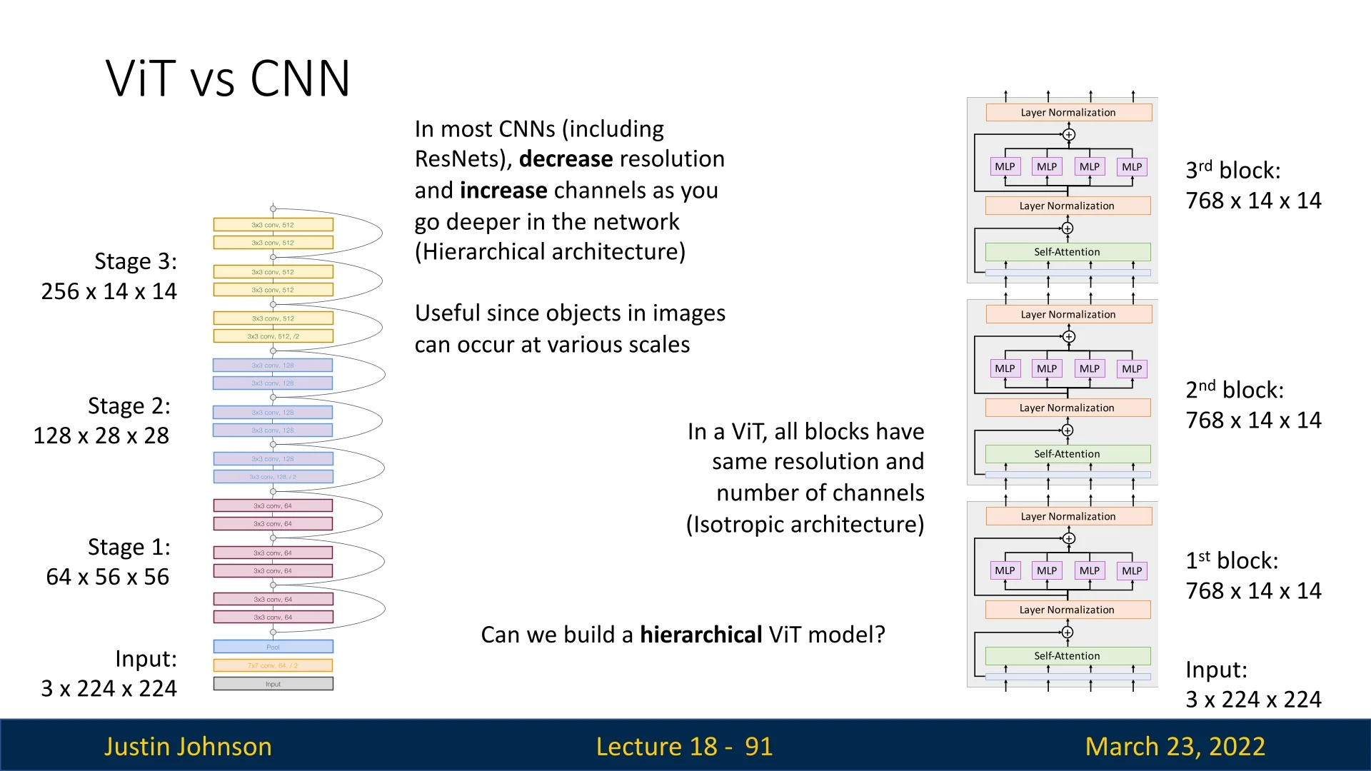
This flat structure poses two practical challenges:
- 1.
- Scaling cost at higher resolution. As input resolution increases with a fixed patch size, the number of tokens grows, making global self-attention increasingly expensive.
- 2.
- Less explicit multi-scale processing. CNNs naturally build coarse-to-fine representations through downsampling stages. DeiT-style models can learn multi-scale behavior, but they must do so without an explicit pyramid of resolutions.
This motivates hierarchical Vision Transformers that recover stage-wise resolution changes while preserving attention-based modeling. The next major step in this direction is the Swin Transformer, which introduces shifted window attention and hierarchical token merging. Swin addresses the high-resolution scaling challenge and provides a more natural foundation for detection and segmentation, while retaining the core benefits of self-attention.
In the next section, we will explore the Swin Transformer and how it resolves key architectural and scaling gaps left by vanilla ViTs and the DeiT family.
18.6 Swin Transformer: Hierarchical Vision Transformers with Shifted Windows
DeiT demonstrated that Vision Transformers can be trained effectively on ImageNet-1k when the training recipe is strengthened and, optionally, supported by a CNN teacher. However, the DeiT family retains the isotropic ViT backbone, and global self-attention remains costly when the input resolution increases. This motivates architectures that preserve Transformer flexibility while introducing hierarchical, multi-scale representations and computationally efficient attention suitable for dense prediction tasks.
The Swin Transformer (Shifted Windows Transformer) [395] addresses this challenge by introducing a hierarchical ViT architecture with two key design principles:
- Local self-attention with non-overlapping windows: Limits self-attention computation to fixed-size windows, significantly reducing computational complexity.
- Shifted windowing scheme: Enables cross-window communication, expanding the effective receptive field and improving the model’s ability to capture long-range dependencies.
This architecture narrows the gap between Vision Transformers and CNNs in terms of efficiency and scalability, enabling their use in dense prediction tasks such as object detection and segmentation. Moreover, Swin achieves strong empirical performance, surpassing earlier ViT and DeiT models on key benchmarks—while preserving linear self-attention complexity with respect to image size for a fixed window size \(M\).
Throughout the following subsections, we will break down the Swin Transformer architecture, drawing primarily on the original paper. Helpful visual intuition and animations are also available in an external walkthrough.1
18.6.1 How Swin Works
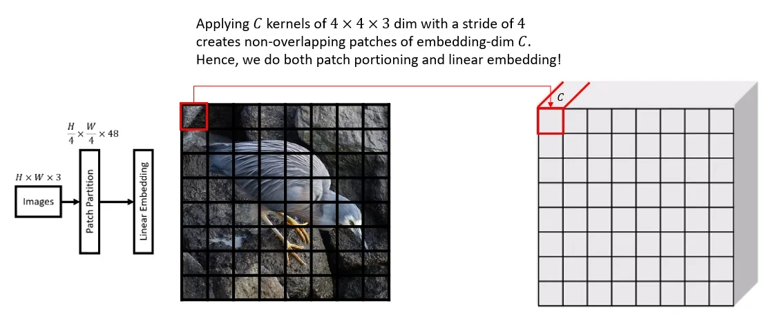
Patch Tokenization As in ViT, an image is split into non-overlapping patches. Swin uses small \(4 \times 4\) patches. Each patch is flattened and linearly projected to a fixed embedding dimension \(C\). This can be implemented efficiently using a convolution layer with:
- Kernel size: \(4 \times 4\).
- Stride: \(4\).
- Number of output channels: \(C\).
This yields a feature map of size \( \frac {H}{4} \times \frac {W}{4} \times C \), where each location corresponds to a token. Equivalently, this converts an input of shape \(H \times W \times 3\) into a token grid of shape \(\frac {H}{4} \times \frac {W}{4} \times C\).
18.6.2 Window-Based Self-Attention (W-MSA)
Instead of computing attention globally (as in ViT), Swin divides the token grid into non-overlapping windows of size \( M \times M \) (e.g., \( M = 7 \)). Within each window, self-attention is computed locally, reducing the total cost.
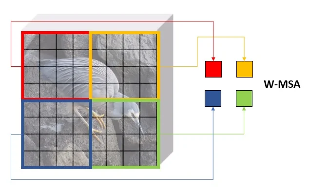
Each window performs self-attention independently:
\begin {equation} \mbox{Self-attention cost per window per layer: } \mathcal {O}(M^4 \cdot C) \end {equation}
Let \( N = \frac {H \cdot W}{16} \) be the number of tokens after \(4 \times 4\) patch embedding, i.e., \(N = \frac {H}{4}\cdot \frac {W}{4}\). The total number of windows is \( \frac {N}{M^2} \), and thus the overall complexity becomes:
\begin {align} \mathcal {O}\left ( \frac {N}{M^2} \cdot M^4 \cdot C \right ) &= \mathcal {O}(N \cdot M^2 \cdot C) \\ &= \mathcal {O}(H \cdot W \cdot C) \quad \text {(since } M \text { is constant)}. \end {align}
Hence, Swin achieves linear complexity with respect to image size.
18.6.3 Limitation: No Cross-Window Communication
While windowed self-attention is efficient, it creates a problem: tokens can only attend to others within the same window. As a result:
- Long-range dependencies across windows are not captured.
- Objects spanning multiple windows may not be modeled holistically.
- Non-adjacent image regions that are semantically linked remain disconnected.
Examples:
- A person’s face partially split across windows may have disconnected features.
- Recognizing symmetry or object boundaries requires context from adjacent or distant windows.
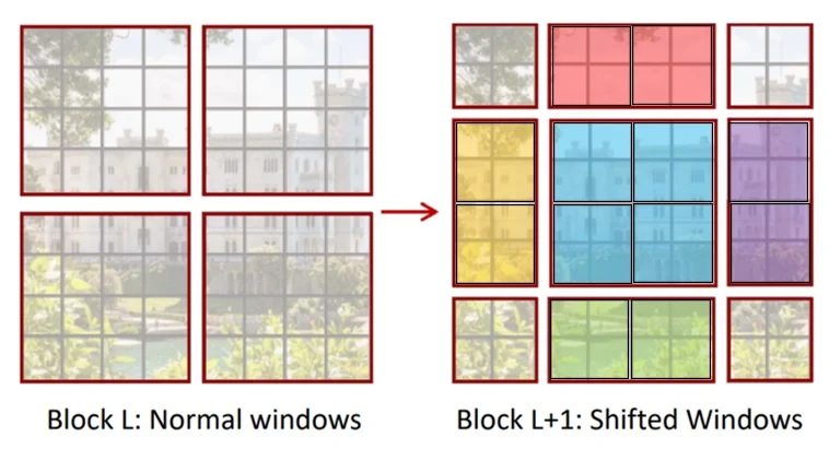
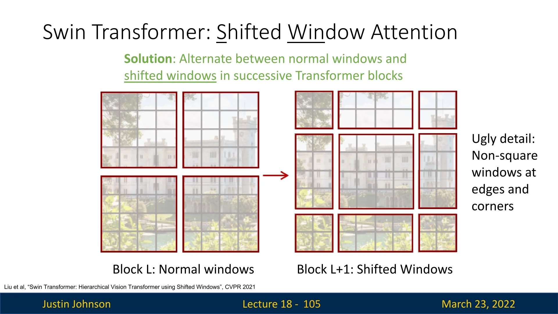
18.6.4 Solution: Shifted Windows (SW-MSA)
Building on the isolation issue of fixed window partitioning, Swin introduces Shifted Window Multi-Head Self-Attention (SW-MSA). Rather than expanding attention beyond \(M \times M\), the model redefines the window grid between consecutive blocks so that windows in the next layer overlap the boundaries of the previous layer. This preserves local attention while creating a structured pathway for cross-window information flow.
- In alternate transformer blocks, the window grid is shifted by \(\lfloor M/2 \rfloor \) patches along both spatial axes.
- The resulting \(M \times M\) windows overlap the boundaries of the previous unshifted windows, so tokens that were previously separated can become co-located.
- Self-attention remains local within each window, but token membership to windows changes across layers, creating a structured route for cross-window information exchange.
Intuitive example: the information-carrier chain To visualize why shifting expands the effective receptive field, consider three patches arranged along a single row of windows:
- Patch A: near the right edge of Window 1.
- Patch B: near the left edge of Window 2, immediately adjacent to A in the original image.
- Patch C: another token inside Window 2, for example near its right edge.
The role of Patch C is to illustrate propagation within and beyond Window 2 once Window 1 and Window 2 have been stitched together.
- 1.
- Block \(L\) (W-MSA: local summaries). Patch A attends to Window 1 and becomes a compact summary of Window 1. Patch B and Patch C attend to Window 2 and become summaries of Window 2. At this point, A does not contain information from Window 2, despite being spatially adjacent to B.
- 2.
- Block \(L{+}1\) (SW-MSA: cross-boundary mixing). After shifting, the old
boundary between Window 1 and Window 2 falls inside a shifted window.
Patch A and Patch B now belong to the same local attention region.
During attention, A and B exchange their window summaries. Ending state
for this pair:
- Patch A now carries information from both Window 1 and Window 2.
- Patch B also carries information from both windows.
- 3.
- Block \(L{+}2\) (propagation within the next local grouping). When the partitioning changes again, a token like Patch B (which now contains Window 1+2 context) can share a window with Patch C (or with a token in Window 3). Thus, B acts as an intermediate carrier: it transfers the combined context onward.
This “bucket-brigade” view explains the receptive-field expansion: tokens first summarize their local window, then exchange those summaries across shifted boundaries, then pass the combined summaries onward. The receptive field is therefore not about a single token directly attending to every distant token in one step, but about progressive context propagation over depth.
Does this achieve global context? In a purely flat windowed transformer, global context would require sufficient depth for information to traverse many window-to-window hops. If the network is too shallow relative to the image size, the effective receptive field can remain partially local.
Swin mitigates this practical limitation with its hierarchical design. Patch merging progressively reduces spatial resolution, so the number of windows shrinks at deeper stages. Consequently, the same fixed window size \(M\) covers a much larger portion of the original image, and later-stage tokens can aggregate near-global context efficiently. In this sense, global understanding in Swin is achieved by the combination of (i) W-MSA/SW-MSA alternation for cross-window connectivity and (ii) patch merging for reducing the spatial distance that context must travel.
- Cross-window communication with local attention: the shift changes token groupings so adjacent windows become connected over depth.
- Progressive context growth: over successive alternations, tokens exchange increasingly rich local summaries, leading to broad effective receptive fields without global attention.
- Linear attention complexity preserved: attention is still computed within \(M \times M\) windows, so for constant \(M\) the per-layer complexity remains \(\mathcal {O}(HWC)\).
Practical challenges of a naive shift The modeling value of SW-MSA is clear, but implementing the shift naively raises boundary and batching complications. Shifting the grid disrupts the regular window tiling near image edges, which would require either padding of irregular boundary regions or separate handling of mismatched window shapes.
These issues motivate a more efficient realization of the same SW-MSA idea, leading to the cyclic implementation described next.
18.6.5 Cyclic Shifted Window-Masked Self Attention (Cyclic SW-MSA)
Shifted windows solve the modeling problem of cross-window communication, but a naive implementation of SW-MSA is inefficient at the image boundaries. The shift disrupts the regular window grid, creating irregular edge regions that would require padding to maintain a fixed \(M \times M\) attention shape. Such padding wastes compute and reduces batching efficiency on modern accelerators.
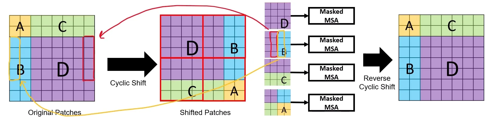
To preserve the modeling benefits of SW-MSA while keeping the computation hardware-friendly, Swin introduces Cyclic Shifted Window Multi-Head Self-Attention (Cyclic SW-MSA). The feature map is treated as toroidal: tokens that would fall beyond one border during the shift are wrapped around to the opposite side. This restores a perfectly regular tiling of \(M \times M\) windows, so shifted attention can be computed in a single efficient batch without boundary padding.
While the connectivity is the same as standard SW-MSA, the cyclic formulation yields practical benefits beyond code elegance: it reduces wasted FLOPs and memory on padded tokens, improves kernel regularity, and can allow larger batch sizes or higher-resolution training under the same compute budget. Because the cyclic roll can place distant regions into the same physical window, an attention mask is applied to ensure that tokens only attend to others that were spatially adjacent in the original, unrolled layout.
- 1.
- Cyclic shift: The token grid is logically shifted so that patches that would have fallen outside the border are wrapped around to the opposite side.
- 2.
- Regular window partitioning: After this roll, the grid can be partitioned into uniform \(M \times M\) windows without zero-padding.
- 3.
- Why masking is still needed: A window in the rolled view may contain patches that were far apart in the original layout. The attention mask prevents these semantically unrelated regions from interacting directly.
This mechanism builds on standard SW-MSA by:
- Applying a cyclic shift to the feature map prior to partitioning into windows.
- Computing attention within fixed-size windows with masking, ensuring only valid, adjacent spatial relationships are attended to.
- Reversing the shift after attention to restore the spatial layout.
Masking in SW-MSA
In SW-MSA, we conceptually want the next attention layer to use windows shifted by \(s=\lfloor M/2 \rfloor \) patches so that each shifted window bridges a boundary from the previous W-MSA partition. This is what enables cross-window information flow while keeping attention local. The subtlety is purely computational: a naive geometric shift produces irregular boundary windows that are awkward to batch. Swin resolves this by implementing the shift via a cyclic roll of the feature map, which restores a regular \(M \times M\) tiling. The price of this efficiency trick is that the rolled feature map may place false neighbors—tokens that were far apart in the unrolled coordinates—inside the same physical window. The attention mask is the mechanism that prevents this implementation device from changing the intended computation graph.
Expanded receptive fields (context reminder) With masking in place, cyclic SW-MSA is equivalent to the conceptual (non-cyclic) SW-MSA layer. Therefore, the receptive-field story is unchanged: alternating W-MSA and SW-MSA lets boundary-crossing information flow accumulate over depth, while each individual attention operation remains local.
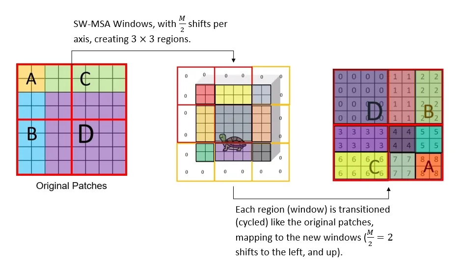
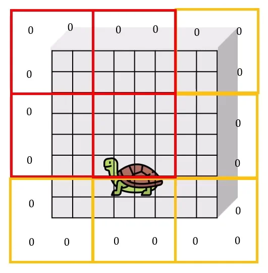
Figure 18.21 disentangles the modeling idea of shifted windows from the efficient implementation used in practice. The left panel groups the toy feature map into four patch regions \(A,B,C,D\), where each region is a set of small patches; in this unshifted layout, each region aligns with one W-MSA window (red outline). The middle panel shows the conceptual shift by \(s=\lfloor M/2 \rfloor \): patches do not move, but the window grid is offset, which logically partitions the map into \(3 \times 3\) sub-regions (IDs \(0\) through \(8\)). These IDs encode which tokens should remain mutually visible under the intended (non-cyclic) shifted-window graph. The right panel illustrates the implementation trick: a cyclic roll restores a regular \(M \times M\) window tiling without padding. Because this roll can pack tokens from different logical IDs into the same physical window, an attention mask is required to preserve the intended locality.
Why the mask is strictly necessary (vs. ViT) One might naturally ask: If Vision Transformers (ViT) allow global attention where all patches communicate, why must we suppress these cross-boundary connections in Swin?
The answer lies in the fundamental architectural difference between Swin and ViT:
- ViT is Isotropic (Global): ViT processes the image as a flat sequence. It is designed to capture global relationships immediately, so connecting any two patches is valid.
- Swin is Hierarchical (Local-to-Global): Swin is designed to mimic the behavior of CNNs. It deliberately restricts attention to local neighborhoods in early layers to capture fine-grained details, only expanding the receptive field gradually through merging and shifting.
Allowing unmasked cyclic connections would not create meaningful global context; it would inject topological noise. True global attention (as in ViT) allows a token to query all other tokens to find semantically relevant dependencies. In contrast, unmasked cyclic attention forces a hard-coded connection to a random, spatially disconnected fragment on the opposite border (e.g., the top-left sky attending to the bottom-right ground) purely as an artifact of the tensor roll. This is not a useful long-range signal; it is a false adjacency. Such arbitrary “wormholes” violate the hierarchical strategy by forcing the model to process unrelated distant regions as neighbors before it has established a coherent local understanding. The mask is therefore required to enforce the local-first logic, ensuring the network builds context step-by-step rather than via accidental implementation shortcuts.
Masked attention formulation Let \(Q,K,V \in \mathbb {R}^{M^2 \times d}\) denote the query, key, and value matrices for one \(M \times M\) window. Cyclic SW-MSA injects an additive mask \(A \in \mathbb {R}^{M^2 \times M^2}\) into the attention logits: \[ \mbox{Attention}(Q,K,V) = \mbox{softmax}\!\Bigl (\tfrac {QK^\top }{\sqrt {d}} + B + A\Bigr )V, \] where \(B\) is the relative position bias. The mask entries satisfy \(A_{ij}=0\) for valid pairs (same logical ID) and \(A_{ij}\ll 0\) for invalid pairs (different logical IDs), so the softmax suppresses attention across cyclicly induced false-neighbor boundaries.
Step-by-step construction of the mask The implementation builds \(A\) by assigning group IDs to the logical partitions induced by the shift:
- 1.
- Assign group IDs to the \(3 \times 3\) partitions.
When shifting by \(s = \lfloor M/2 \rfloor \), the feature map can be decomposed into three bands along height and three bands along width: \[ [0, H{-}M),\quad [H{-}M, H{-}s),\quad [H{-}s, H). \] Their Cartesian product yields \(3 \times 3\) regions. Each region receives a unique integer ID.
H, W = self.input_resolution
M = self.window_size
s = self.shift_size  # typically M // 2

img_mask = torch.zeros((1, H, W, 1))  # 1 x H x W x 1

h_slices = (slice(0, -M),
            slice(-M, -s),
            slice(-s, None))
w_slices = (slice(0, -M),
            slice(-M, -s),
            slice(-s, None))

cnt = 0
for h in h_slices:
    for w in w_slices:
        img_mask[:, h, w, :] = cnt
        cnt += 1
Interpretation: tokens with the same ID belong to the same logical partition in the non-cyclic shifted layout.
- 2.
- Apply the cyclic shift and partition into windows.
shifted_mask = torch.roll(img_mask, shifts=(-s, -s), dims=(1, 2))

mask_windows = window_partition(shifted_mask, M)  # nW x M x M x 1
mask_windows = mask_windows.view(-1, M * M)       # nW x M^2
After the roll, each physical \(M \times M\) window may contain multiple IDs.
- 3.
- Generate the additive attention mask.
attn_mask = mask_windows.unsqueeze(1) - mask_windows.unsqueeze(2)
attn_mask = attn_mask.masked_fill(attn_mask != 0, float(-100.0))
attn_mask = attn_mask.masked_fill(attn_mask == 0, float(0.0))
Interpretation: two tokens are allowed to attend only if their IDs match. Otherwise, the mask injects a large negative penalty.
Why \(-100.0\) is sufficient in practice In attention, \[ \mbox{softmax}(A_{ij}) = \frac {\exp (A_{ij})}{\sum _k \exp (A_{ik})}. \] With typical floating-point ranges, \(\exp (-100)\) is effectively zero, so masked pairs contribute negligible probability. This is a stable finite approximation of adding \(-\infty \).
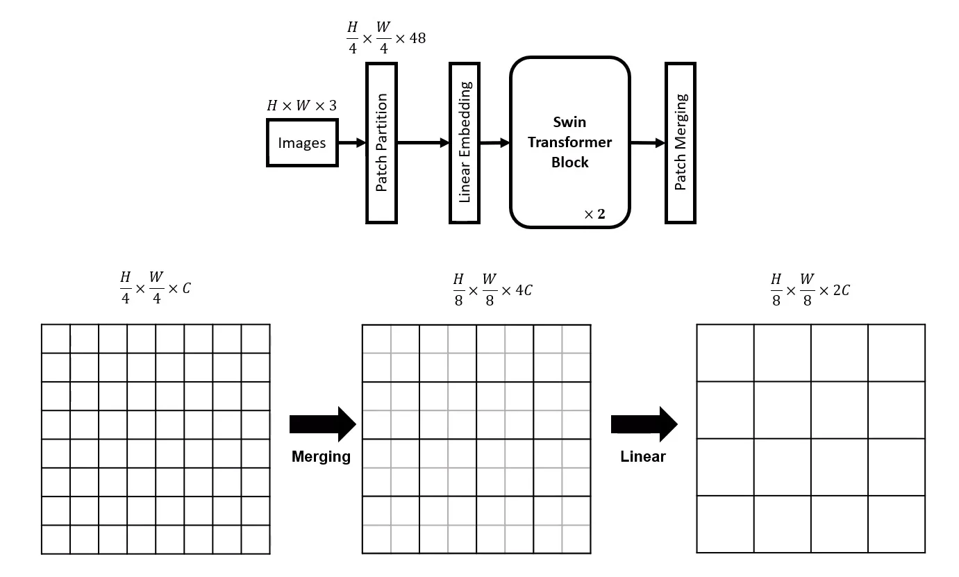
18.6.6 Patch Merging in Swin Transformers
One of the core architectural innovations in Swin Transformers is the patch merging mechanism. Unlike ViT, which maintains a fixed token resolution across all layers, Swin progressively reduces spatial resolution in a hierarchical fashion, analogous to spatial downsampling in CNNs (e.g., max pooling or strided convolutions). This allows deeper layers to operate on coarser representations, increasing both computational efficiency and receptive field.
What Happens in Patch Merging?
- The feature map is divided into non-overlapping \(2 \times 2\) spatial groups.
- The embeddings of the four patches in each group are concatenated: \[ [\mathbf {x}_1, \mathbf {x}_2, \mathbf {x}_3, \mathbf {x}_4] \in \mathbb {R}^{4C}. \]
- A linear projection reduces the dimensionality from \(4C\) to \(2C\): \[ \mathbf {y} = W_{\mbox{merge}} \cdot [\mathbf {x}_1; \mathbf {x}_2; \mathbf {x}_3; \mathbf {x}_4], \quad W_{\mbox{merge}} \in \mathbb {R}^{2C \times 4C}. \]
Benefits of Patch Merging
- Hierarchical Representation: Enables the model to learn multi-scale features across different stages, from fine details to coarse semantics—similar to CNNs.
- Context Expansion via SW-MSA: As Swin blocks are stacked, the combination of patch merging and shifted window attention allows more distant patches to interact. Even though W-MSA starts with small local windows, successive blocks expand the model’s receptive field, enabling global reasoning over time.
- Computational Efficiency: Reducing the number of tokens at deeper layers significantly lowers the cost of self-attention, especially compared to flat-resolution ViTs.
- Empirical Performance: Despite using small initial patch sizes (e.g., \(4 \times 4\)), Swin Transformers often outperform ViTs using coarser patches (e.g., \(16 \times 16\))—due to the combination of local precision and effective hierarchical abstraction.
Downsides and Considerations
- Spatial Detail Loss: Each merging step reduces spatial granularity, which may obscure fine structures—though this is often compensated for by higher-level context aggregation.
- Increased Channel Dimensionality: Doubling feature dimensions increases parameter count and projection cost.
- Less Uniform Design: Unlike ViT’s isotropic (uniform) architecture, Swin’s stage-wise structure adds design complexity and requires reasoning across multiple resolutions.
Nonetheless, this architectural shift is central to Swin’s success. The combined effect of hierarchical patch merging and shifted window self-attention enables Swin Transformers to scale efficiently and generalize well—bridging the gap between CNN-style design and transformer flexibility.
18.6.7 Positional Encoding in Swin Transformers
In standard Vision Transformers (ViTs), each patch embedding \(\mathbf {x}_i \in \mathbb {R}^{D}\) is enriched with a learnable absolute position encoding \(\mathbf {p}_i\): \[ \mathbf {z}_i = \mathbf {x}_i + \mathbf {p}_i, \] which treats each patch as having a unique coordinate in the global image grid. While effective for fixed-resolution inputs, absolute position embeddings struggle with hierarchical architectures where resolution changes, and they do not generalize well if the image size varies at inference time.
Relative Position Bias in Swin Transformers Rather than adding a global absolute positional embedding to each token, Swin encodes spatial structure locally inside each window via a relative position bias \(B\) added to the attention logits [395]. For a window of size \(M \times M\), attention is computed as: \[ \mbox{Attention}(Q,K,V) = \mbox{softmax}\!\Bigl (\frac {QK^\top }{\sqrt {C}} + B\Bigr )V. \] Here \(B\) is implemented as a learnable lookup table indexed by the relative offset \((\Delta r, \Delta c)\) between two tokens. Because attention is restricted to a local window, the set of possible offsets is finite: \[ \Delta r, \Delta c \in \{-(M-1), \ldots , (M-1)\}, \] so the table contains exactly \((2M-1)^2\) entries.
Why a lookup table? (Bias vs. Sinusoid) A learned table is a natural match for window attention:
- Finite offset domain: For a typical window size \(M=7\), there are only \(13^2 = 169\) unique relative positions. A small table is computationally efficient and sufficient to cover all possible within-window spatial relationships.
- Head-specific locality: A learnable bias allows each attention head to emphasize distinct local patterns, for example prioritizing immediate vertical neighbors while suppressing diagonals. This discrete flexibility is harder to express with the smooth functional form of sinusoidal embeddings.
Hierarchical consistency: Token-space vs. pixel-space A common source of confusion is why this fixed \(M \times M\) bias parameterization remains valid as the network gets deeper and the spatial resolution shrinks. The key is to separate two notions of distance:
- Topological distance (Tokens): Within any Swin block, self-attention is always computed over a discrete \(M \times M\) grid of tokens. The bias table is parameterized purely in this token coordinate system.
- Physical distance (Pixels): After Patch Merging, a single token represents a larger region of the original image. However, the attention mechanism is “blind” to this physical footprint and only operates on the token grid.
Intuitively, the hierarchy acts like a controlled zooming out. In early stages, “one token to the right” corresponds to a small pixel displacement and helps model fine structure. In later stages, the same topological relation links coarser, semantically richer units because each token already summarizes a larger area. Thus, the relative geometry indexed by \((\Delta r,\Delta c)\) remains a stable structural concept even as the physical receptive field grows.
Why relative position bias fits hierarchical Transformers
- Translation invariance: By conditioning attention on relative offsets \((\Delta r,\Delta c)\) rather than absolute coordinates, local interactions depend on relative spatial relationships, not on where features sit in the global image grid.
- Resolution-agnostic inference: Because the bias depends on the window size \(M\) (a hyperparameter) rather than the image size \(H \times W\), a Swin model trained on \(224 \times 224\) inputs can be applied to substantially larger images without interpolating absolute positional embeddings.
Implementation detail Internally, the bias is stored as a parameter table \(\hat {B} \in \mathbb {R}^{(2M-1)\times (2M-1)}\). To materialize the bias matrix \(B\) for a specific window, we compute all pairwise relative coordinates for the \(M^2\) tokens, shift indices to be non-negative, and map them to entries in \(\hat {B}\).
Limitation and evolution toward Swin V2 The lookup-table approach assumes a fixed window size \(M\). If we wish to transfer a model to a task that benefits from larger windows (e.g., increasing \(M\) from \(7\) to \(12\)), the discrete table lacks parameters for the new offsets. This limitation motivates Swin V2, which replaces the static table with a Log-spaced Continuous Position Bias (Log-CPB), allowing smoother extrapolation to unseen window sizes while preserving the local, hierarchical design of Swin.
18.6.8 Conclusion: The Swin Transformer Architecture and Variants
Swin Transformer introduced a compelling shift in vision transformer design by combining the benefits of self-attention with a hierarchical structure—a feature previously reserved for convolutional networks. This enables efficient multi-scale representation learning and significantly enhances the transformer’s ability to model fine-grained local and global patterns.
Overall Swin Architecture
By combining the hierarchical downsampling of CNNs with the dynamic feature interaction of Transformers, Swin bridges the gap between the two paradigms. Its backbone alternates local context aggregation (W-MSA) with cross-window mixing (SW-MSA) and inserts patch merging between stages to build a compact multi-scale feature pyramid. This design preserves strong accuracy while enabling efficient scaling to higher resolutions and dense prediction tasks.
In terms of shapes, patch merging transforms \(\frac {H}{4}\times \frac {W}{4}\times C\) tokens into \(\frac {H}{8}\times \frac {W}{8}\times 2C\).
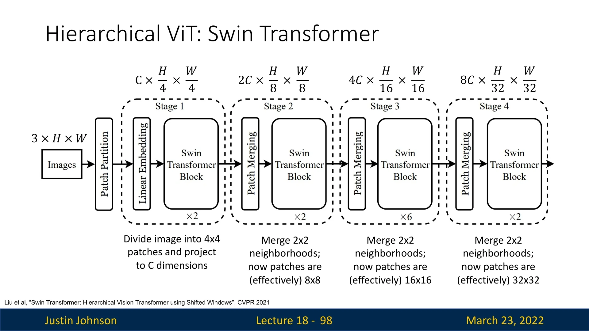
Swin Variants (T/S/B/L)
Swin Transformer comes in different sizes analogous to the ViT family (Tiny, Small, Base, and Large). The table below summarizes the architecture of each variant:
| Stage | Downsample Rate | Swin-T | Swin-S | Swin-B | Swin-L |
|---|---|---|---|---|---|
| Stage 1 | \(4\times \) (\(56\times 56\)) | dim 96 2 blocks head 3 | dim 96 2 blocks head 3 | dim 128 2 blocks head 4 | dim 192 2 blocks head 6 |
| Stage 2 | \(8\times \) (\(28\times 28\)) | dim 192 2 blocks head 6 | dim 192 2 blocks head 6 | dim 256 2 blocks head 8 | dim 384 2 blocks head 12 |
| Stage 3 | \(16\times \) (\(14\times 14\)) | dim 384 6 blocks head 12 | dim 384 18 blocks head 12 | dim 512 18 blocks head 16 | dim 768 18 blocks head 24 |
| Stage 4 | \(32\times \) (\(7\times 7\)) | dim 768 2 blocks head 24 | dim 768 2 blocks head 24 | dim 1024 2 blocks head 32 | dim 1536 2 blocks head 48 |
This hierarchical structure with progressive patch merging not only boosts accuracy but also enables efficient training and inference on dense prediction tasks.
Speed vs. Accuracy: Swin vs. DeiT and CNNs
Swin Transformers offer a compelling balance between speed and accuracy compared to other vision models such as DeiT, EfficientNet, and RegNetY. This is largely due to their hierarchical design, efficient windowed attention, and flexible scaling strategies.
Unlike vanilla ViTs and DeiT, which operate on fixed-size \(16 \times 16\) patches and maintain uniform resolution across layers (isotropic architecture), Swin operates on small \(4 \times 4\) patches and hierarchically merges them, forming a multi-resolution feature pyramid. This enables it to process both fine and coarse visual patterns efficiently.
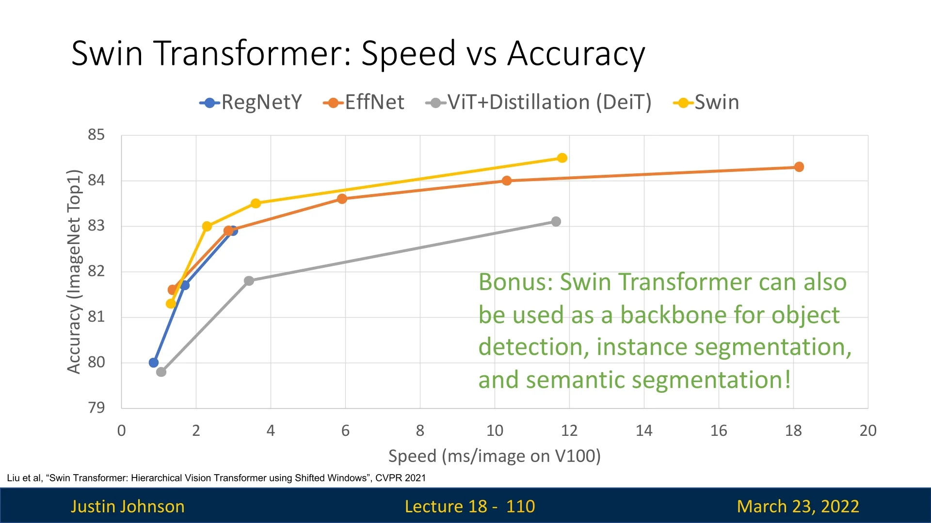
Thanks to its linear computational complexity, Swin can be scaled to higher resolutions without a quadratic memory or latency blow-up, making it suitable for dense vision tasks such as semantic segmentation, object detection, and keypoint estimation.
18.7 Extensions and Successors to Swin
The Swin Transformer’s core ideas—hierarchical feature maps, local window-based attention, and shifted window partitioning—have motivated a broad family of follow-up architectures. Among these, Swin Transformer V2 [394] is the most direct and principled evolution of the original design. Its main goal is not to change Swin’s core hierarchical, windowed recipe, but to make this recipe scale: Swin V2 targets the numerical and systems bottlenecks that emerge when we push Swin-style models to much larger capacities and much higher input resolutions.
Empirically, Swin V1 already delivers strong performance at common ImageNet-scale settings. However, naive scaling exposes two recurring issues: (1) attention logits can become excessively sharp or unstable as feature magnitudes grow with depth and width, and (2) the discrete relative-position table becomes an awkward parameterization when transferring to new window sizes or fine-tuning at substantially higher resolutions. Swin V2 addresses these issues with three architectural changes, complemented by training and implementation practices that make extreme scaling feasible.
18.7.1 Swin Evolution: Swin Transformer V2
Swin Transformer V2 [394] is a direct evolution of Swin V1 that preserves the hierarchical, windowed backbone while addressing two practical scaling barriers: unstable attention behavior when capacity grows and brittle relative-position parameterization when window size or fine-tuning resolution changes. To target these failure modes, V2 introduces three architectural adjustments that are designed to be drop-in compatible with the original Swin stages.
- Residual Post-Norm. Normalizes the residual branch output before it is added to the identity path, reducing activation drift as depth and width increase.
- Scaled Cosine Attention. Computes attention logits from cosine similarity with a learnable temperature, limiting sensitivity to the magnitude of \(Q\) and \(K\).
- Log-Spaced Continuous Position Bias (Log-CPB). Replaces the discrete relative-bias table with a small meta-network evaluated on log-spaced relative coordinates, enabling smoother transfer across window sizes.
Taken together, these modifications keep the original Swin computation pattern but make it feasible to train much larger models and to fine-tune them at substantially higher input and window resolutions.
1) Scaled Cosine Attention Within each window, Swin V1 computes scaled dot-product attention: \[ \operatorname {Attention}(Q,K,V) = \operatorname {softmax}\!\Bigl (\tfrac {QK^\top }{\sqrt {C}} + B\Bigr )V, \] where \(Q,K,V \in \mathbb {R}^{M^2 \times C}\) are the query, key, and value matrices for one \(M \times M\) window, \(C\) is the per-head channel dimension, and \(B\) is the relative position bias. At large scale, the norms of \(Q\) and \(K\) may vary widely across layers, causing logits to become overly sharp and making optimization more fragile.
Swin V2 replaces the dot-product similarity with a scaled cosine formulation: \[ \operatorname {CosineAttention}(Q,K,V) = \operatorname {softmax}\!\Bigl (\tfrac {\operatorname {cos}(Q,K)}{\tau } + B\Bigr )V, \] with the pairwise similarity defined token-wise as \[ \operatorname {Sim}(q_i,k_j) = \frac {\langle q_i,k_j\rangle }{\|q_i\|\|k_j\|}\cdot \frac {1}{\tau } + B_{ij}. \] Here \(q_i\) and \(k_j\) are rows of \(Q\) and \(K\), and \(\tau >0\) is a learnable temperature. Because cosine similarity is bounded in \([-1,1]\), the logits are no longer directly amplified by feature magnitude. The learnable \(\tau \) then provides a controlled mechanism for setting attention sharpness, rather than letting sharpness be an accidental byproduct of scale.
2) Log-Spaced Continuous Position Bias (Log-CPB) Swin V1 encodes local relative geometry using a discrete lookup table with \((2M-1)^2\) entries. This is efficient for a fixed \(M\), but when the window size changes between pretraining and fine-tuning, the table must be interpolated, which is an awkward operation for a set of categorical bias parameters.
Swin V2 introduces a continuous bias generator. For a pair of tokens with relative offset \((\Delta x,\Delta y)\), V2 first transforms the coordinates to log-space: \[ \hat {\Delta x} = \operatorname {sign}(\Delta x)\log \!\bigl (1+|\Delta x|\bigr ), \qquad \hat {\Delta y} = \operatorname {sign}(\Delta y)\log \!\bigl (1+|\Delta y|\bigr ), \] and then predicts the bias using a small MLP \(\mathcal {G}\): \[ B(\Delta x,\Delta y) = \mathcal {G}(\hat {\Delta x},\hat {\Delta y}). \] This Log-CPB parameterization follows the formulation introduced in Swin V2.
Operationally, this change:
- Reduces parameter growth. The bias no longer scales quadratically with \(M\) because it is produced by a fixed-size meta-network.
- Improves transfer across window sizes. Log-spaced coordinates reduce the effective extrapolation gap when increasing \(M\), which improves fine-tuning stability at higher resolutions.
- Encourages smooth spatial behavior. Bias values vary as a learned function of displacement rather than as unrelated table entries.
3) Residual Post-Norm A key instability observed when scaling Swin V1 is activation accumulation along residual paths. In abstract form, a V1-style pre-norm residual unit can be written as \[ x_{\mbox{out}} = x + F\!\bigl (\operatorname {LayerNorm}(x)\bigr ), \] where \(F(\cdot )\) denotes the transformation inside the residual branch. In Swin blocks, \(F\) is instantiated by either a window attention module (W-MSA or SW-MSA) or the two-layer MLP sub-block.
When capacity grows, the magnitude of the branch output \(F(\cdot )\) can drift upward across depth. Even though the identity path \(x\) is still present, repeatedly adding an uncontrolled update can inflate activation variance layer-by-layer. This inflation then feeds back into attention and MLP computations, making the training dynamics increasingly brittle.
Swin V2 addresses this with Residual Post-Norm: \[ x_{\mbox{out}} = x + \operatorname {LayerNorm}\!\bigl (F(x)\bigr ). \] This differs from the classical post-norm form \(\operatorname {LayerNorm}(x+F(x))\). Here the identity path remains unnormalized and therefore provides a stable reference signal, while the update is explicitly normalized before being merged. As a result, the scale of the residual updates is kept consistent across depth. The paper also notes that for the largest variants an additional \(\operatorname {LayerNorm}\) is inserted on the main branch every 6 Transformer blocks to further stabilize training.
4) Scaling beyond architecture: training and systems considerations The Swin V2 study emphasizes that these architectural changes are complemented by training and systems choices needed for extreme regimes, including self-supervised masked image modeling (e.g., SimMIM) and memory-aware implementations such as optimizer-state sharding, activation checkpointing, and more memory-efficient attention computation at high resolutions.
Implications and results Swin V2 answers a practical scaling question: How can we keep the hierarchical, windowed Swin recipe while pushing to far larger models and much higher resolutions? Scaled cosine attention limits logit extremes, Log-CPB removes the brittleness of a fixed lookup table, and residual post-norm constrains activation drift. Together, these changes enable stable training and effective transfer of large Swin backbones while preserving the linear-in-image-size efficiency that motivates window attention in the first place.
18.7.2 Multiscale Vision Transformer (MViT)
Multiscale Vision Transformers (MViT) [152] introduce a hierarchical Transformer backbone designed for high-resolution visual inputs, especially long video sequences where token counts can be extreme. The central idea is to build a feature pyramid inside the Transformer. Instead of preserving a single token grid throughout the network as in standard ViTs, MViT progressively reduces spatial (or spatiotemporal) resolution across stages while increasing channel capacity. This stage-wise resolution–channel tradeoff parallels the design pattern of strong CNN backbones and makes MViT particularly suitable for dense prediction pipelines that expect multi-scale features.
1. Pooling Attention (MHPA) The engine behind this hierarchy is Multi-Head Pooling Attention (MHPA). Standard self-attention operates on queries \(Q\), keys \(K\), and values \(V\) of identical sequence length \(L\), yielding an \(O(L^2)\) attention matrix. At high spatial resolution, and even more so for video with \(L \propto T \cdot H \cdot W\), this quadratic cost becomes a primary bottleneck. MHPA introduces learnable pooling operators that may downsample the three tensors: \[ Q,\, K,\, V \;\;\longrightarrow \;\; \mathcal {P}_Q(Q),\; \mathcal {P}_K(K),\; \mathcal {P}_V(V), \] yielding an attention computation of the form \[ \operatorname {MHPA}(Q,K,V) = \operatorname {softmax}\!\Bigl ( \frac { \mathcal {P}_Q(Q)\,\mathcal {P}_K(K)^\top }{ \sqrt {d} } \Bigr )\, \mathcal {P}_V(V), \] where \(d\) is the per-head dimension.
A key conceptual point is that pooling serves two distinct roles in MViT [152]:
- Resolution Downsampling (Pooling \(Q\)). Pooling the queries reduces the output token length and is therefore used to downsample the representation at the start of a new stage. This is the mechanism that creates the internal pyramid.
- Compute Reduction (Pooling \(K,V\)). Pooling the keys and values compresses the context that each query attends to, reducing the attention matrix size and memory footprint without necessarily changing the output resolution of the block.
In practice, MViT uses this separation to maintain a global receptive field. Keys and values can be pooled broadly to reduce cost, while query pooling is applied more selectively to control when and how the representation is downsampled across stages.
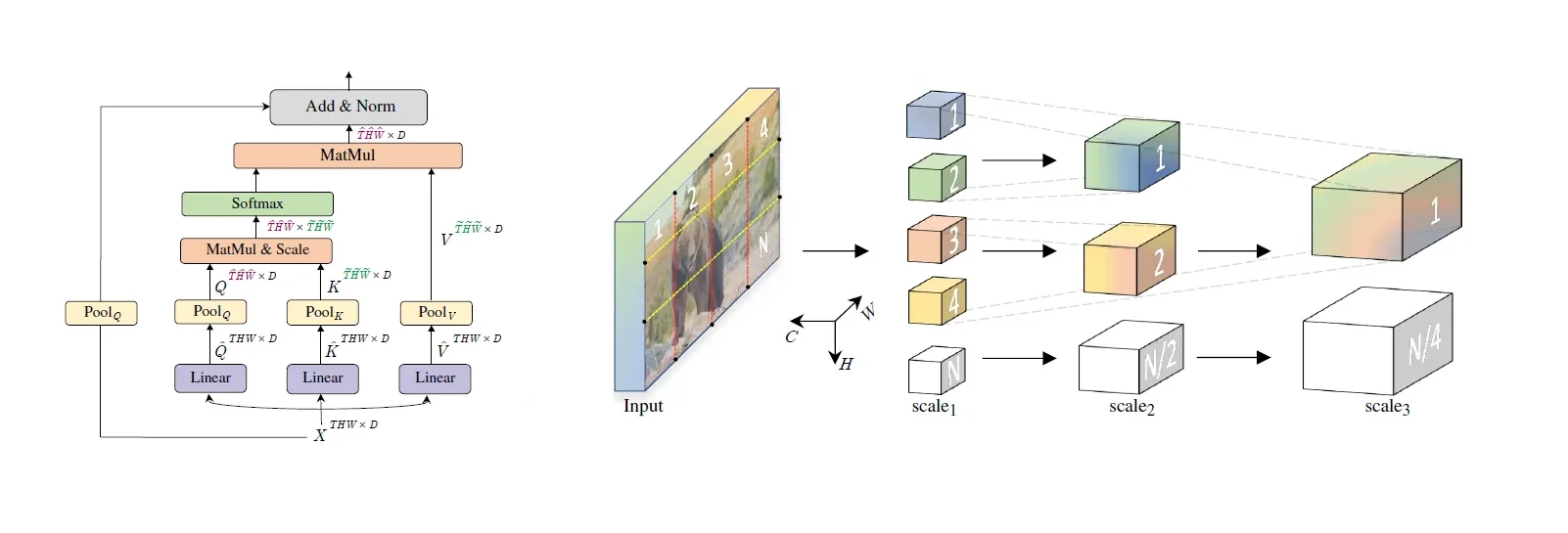
Figure 18.25 highlights that pooling is applied after projection and can be configured differently for \(Q\) versus \(K,V\). This decoupling is what allows MViT to preserve long-range interactions while still constructing a pyramidal hierarchy.
How does pooling work in space and time? Each tensor \(Q, K, V \in \mathbb {R}^{L \times D}\) can be reshaped into a 4D grid \((T, H, W, D)\), where:
- Temporal Extent \(T\). \(T\) is the number of frames for video inputs and defaults to \(1\) for images.
- Spatial Grid \(H \times W\). \(H \times W\) is the token lattice at the current stage.
- Embedding Width \(D\). \(D\) is the token channel dimension.
Pooling is typically implemented with strided, overlapping operators (often convolutional), which summarize local neighborhoods rather than discarding tokens outright. A \(3 \times 3\) kernel with stride \(2\), for example, provides a CNN-like downsampling effect while maintaining smoother information flow across adjacent regions.
2. Hierarchical token downsampling across stages Beyond per-block pooling, MViT organizes the backbone into stages. Within a stage, several Transformer blocks operate at a fixed resolution. At a stage transition, the first block applies query pooling and projection to reduce token resolution and increase channels: \[ (\mbox{Resolution}, \mbox{Channels}) \;:\; (56 \times 56, 96) \longrightarrow (28 \times 28, 192). \] This stage-wise structure yields multi-scale feature outputs that plug naturally into detector and segmenter heads.
3. Global attention with controlled token budgets Unlike Swin, which enforces locality through non-overlapping windows, MViT retains global attention as the conceptual default for its v1 design. The model manages cost by strategically reducing token counts via pooling rather than restricting the attention graph itself. This yields a clean division of labor:
- High-Resolution Early Processing. Early stages preserve dense token grids to capture fine structure.
- Low-Resolution Semantic Aggregation. Deeper stages operate on fewer tokens with higher channel capacity.
- Global Context At Each Scale. Pooling reduces quadratic cost while keeping long-range interactions feasible.
Originally designed for video, effective for images MViT was first motivated by the extreme sequence lengths of video. However, the same multiscale pooling strategy transfers well to images and provides an efficient hierarchical alternative to fixed-resolution ViTs in both classification and dense prediction settings [152].
Empirical strengths Across classification and dense benchmarks, the original MViT family demonstrates that multiscale pooling can deliver strong accuracy with substantially reduced compute at high resolutions [152]. Key practical takeaways include:
- Efficiency At Scale. Token reduction in deeper layers lowers FLOPs and memory demands for high-resolution inputs.
- Competitive Accuracy–Efficiency Tradeoffs. Pooling attention provides a strong alternative to window-restricted attention when a global receptive field is desirable.
- Natural Compatibility With Pyramid Heads. Multi-scale outputs align well with FPN-style detection and segmentation pipelines.
18.7.3 Improved Multiscale Vision Transformers: MViTv2
MViTv2 [354] refines the original design to improve training stability, reduce positional-encoding overhead, and strengthen performance on high-resolution dense tasks. The paper’s empirical ablations emphasize three complementary upgrades: Decomposed relative positional embeddings, Residual pooling connections, and a task-aware Hybrid Window Attention strategy for the largest detection regimes.
1. Decomposed relative positional embeddings
MViT v1 primarily relies on absolute positional embeddings. MViTv2 shows that absolute position provides only modest gains over no positional encoding in this architecture, in part because the convolutional pooling operators already inject spatial structure [354]. To obtain stronger shift-consistent improvements without the heavy cost of joint space–time tables, MViTv2 adopts decomposed relative positional embeddings that factor space and time into separable components.
Concretely, the relative embedding between token \(i\) and \(j\) is expressed as a sum of axis-wise terms: \[ R_{p(i), p(j)} = R^{(\mathrm {h})}_{h(i), h(j)} + R^{(\mathrm {w})}_{w(i), w(j)} + R^{(\mathrm {t})}_{t(i), t(j)}, \] with the temporal term omitted for image-only settings. This design reduces the overhead of positional modeling to a linear-in-axis form while preserving the benefits of relative geometry for dense tasks [354].
2. Residual pooling connections
Aggressive query pooling is essential for building the MViT hierarchy, but it can weaken gradient flow and feature continuity at stage transitions. MViTv2 addresses this with a residual pooling connection that adds a skip from the pooled query stream back to the attention output: \[ Z = \operatorname {Attn}(Q, K, V) + Q_{\mbox{pooled}}. \] Because the skip uses the pooled query, the tensor shapes match naturally. Ablations show that this residual path improves both ImageNet and COCO performance with negligible cost, especially when paired with the stage-wise \(Q\)-pooling design of MViTv2 [354].
3. Hybrid Window Attention (Hwin)
For very high-resolution detection, even pooling attention can become expensive. To compete directly with window-based backbones in this regime, MViTv2 introduces Hybrid Window Attention. The strategy is simple and stage-aware: most blocks in a stage use local window attention for efficiency, but the final blocks of the later stages revert to pooling attention to re-inject global context before features are exported to FPN-style heads [354]. This preserves MViT’s global-information advantage while achieving a more favorable accuracy–throughput balance at detection-scale resolutions.
Performance benefits
Overall, MViTv2 strengthens the original multiscale blueprint:
- Improved Positional Modeling. Decomposed relative embeddings provide shift-consistent gains with lower memory and faster training than joint relative schemes.
- More Stable Hierarchy Construction. Residual pooling improves stage-transition optimization and boosts accuracy on both classification and detection.
- Flexible Global–Local Tradeoffs. Hybrid Window Attention enables efficient scaling to the largest dense-resolution settings while retaining global-context refresh points.
Summary
MViTv2 refines how multiscale attention is implemented rather than departing from the MViT philosophy:
- Decompose Relative Geometry. Factor space and time biases to reduce overhead while preserving shift-consistent benefits.
- Stabilize Pooled Stages. Add residual pooling paths so aggressive \(Q\)-downsampling does not disrupt optimization.
- Mix Attention Scopes When Needed. Combine local windows with pooling attention to balance efficiency and global context for dense tasks.
Looking ahead The progression from ViT to Swin and MViT illustrates two complementary strategies for making Transformers practical for high-resolution vision: restrict the attention graph (windowed attention), or reduce the token budget (pooling attention). Both approaches recover multi-scale backbones that integrate naturally with modern detection and segmentation systems.
But what if we step away from attention altogether?
Can we design vision models that match Transformer-level performance without any attention mechanism—using only MLPs?
This idea led to the MLP-Mixer [639], a simplified architecture that removes both attention and convolutions. Instead, it alternates token-mixing and channel-mixing MLPs to enable global interaction in a purely feed-forward manner. In the next section, we examine this design and the assumptions under which such a minimal mixing mechanism can still perform competitively.
18.8 MLP-Mixer: All-MLP Vision Architecture
Until now, the architectures we have explored—ViT, DeiT, Swin, MViT, and MViTv2—rely on self-attention (or attention variants) as the key primitive for spatial information exchange. In contrast, MLP-Mixer [639] asks a deliberately minimal question: How far can we go if we remove both convolutions and attention, and keep only MLPs? The answer is an “existence proof” that competitive vision models can be built using only feed-forward blocks, provided that training scale and regularization are sufficiently strong.
18.8.1 The MLP-Mixer Architecture
MLP-Mixer follows the ViT input protocol. Given an image, we partition it into \(N\) non-overlapping patches of size \(P \times P\). Each patch is flattened and linearly projected into a \(C\)-dimensional embedding, producing an input table: \[ X \in \mathbb {R}^{N \times C}. \] Unlike standard ViTs, MLP-Mixer does not rely on a class token (‘[CLS]’) as the default aggregation mechanism. Instead, the final prediction is typically formed by global average pooling over the \(N\) tokens, followed by a linear classifier [639].
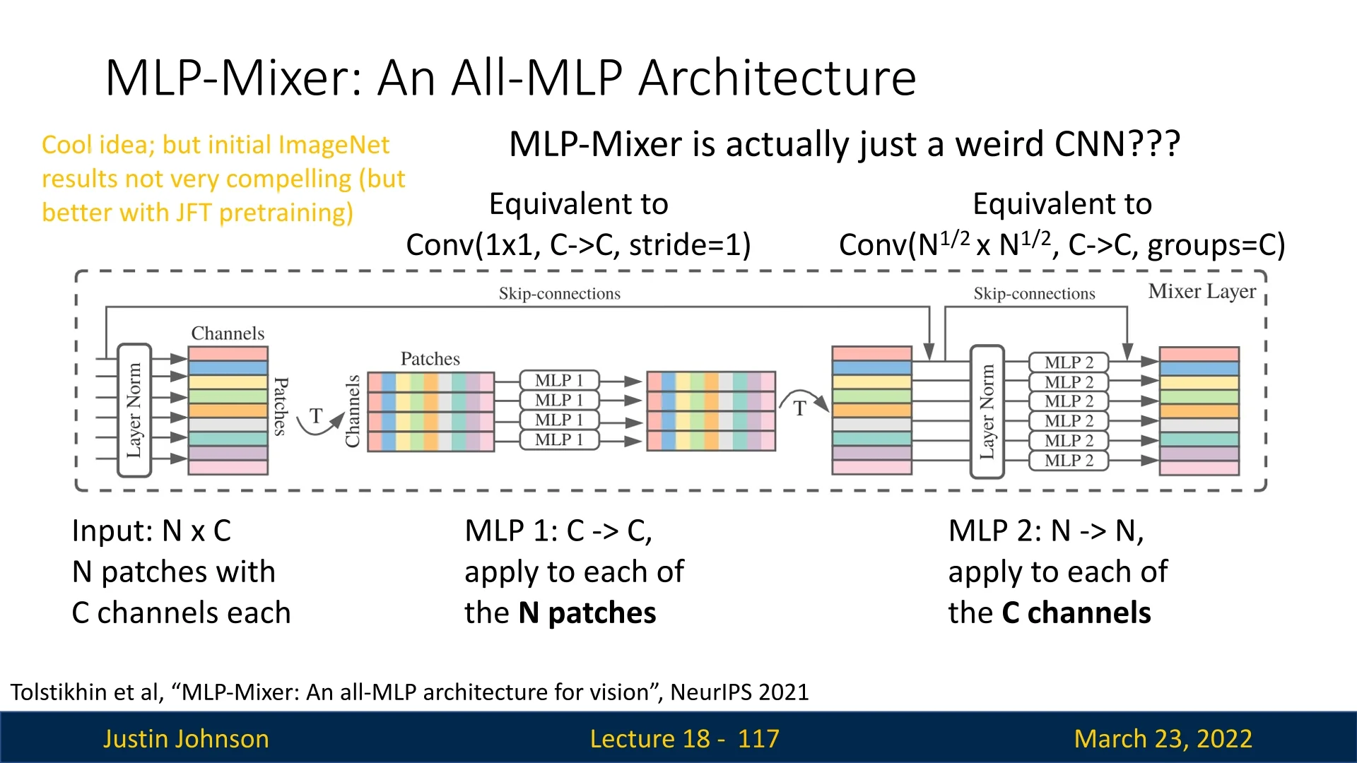
Mixer layers: separating token and channel communication
As illustrated in Figure 18.26, the Mixer layer abandons self-attention in favor of two orthogonal Multi-Layer Perceptron (MLP) blocks. The architecture treats the input strictly as a table of \(N\) patches \(\times \) \(C\) channels. The layer alternates between mixing feature information and mixing spatial information:
- 1.
- Channel-mixing MLP (MLP 1): Applied to each patch independently, mixing features \(C \to C\).
- 2.
- Token-mixing MLP (MLP 2): Applied to each channel independently, mixing spatial locations \(N \to N\).
1) Channel-mixing MLP (Feature Mixing) The first block (labeled MLP 1 in Figure 18.26) operates on the rows of the input matrix. It projects the \(C\) channels to a new feature space and back. Mathematically, for an input \(U\), this is: \begin {align} Y &= U + W_2 \cdot \sigma (W_1 \cdot \text {LN}(U)) \label {eq:channel_mix} \end {align}
where \(W_1, W_2\) act on the dimension \(C\). This operation applies the same MLP to every patch.
Intuition: This is mathematically equivalent to a standard \(1 \times 1\) convolution with stride 1, mapping \(C \to C\). It allows the model to reason about what is at a specific location (e.g., ”is this pixel red?”) but does not look at neighbors.
2) Token-mixing MLP (Spatial Mixing) The second block (labeled MLP 2 in Figure 18.26) enables spatial interaction. Because standard dense layers operate on the last dimension, the Mixer transposes the input matrix (denoted by the arrow \(T\) in the figure) to align the \(N\) patches with the MLP dimension. \begin {align} U &= X + (W_4 \cdot \sigma (W_3 \cdot \text {LN}(X)^\top ))^\top \label {eq:token_mix} \end {align}
Here, the weights \(W_3, W_4\) act on the dimension \(N\). Crucially, these weights are shared across all \(C\) channels.
Intuition: This is equivalent to a single-channel depthwise convolution (groups=\(C\)) with a receptive field covering the entire image (kernel size = image size). It allows the model to reason about where things are (e.g., ”move information from the top-left corner to the center”) using a fixed spatial pattern.
Is MLP-Mixer just a ”Weird CNN”?
The slide poses a provocative question: ”MLP-Mixer is actually just a weird CNN?”. The answer lies in the specific parameter sharing structure and kernel sizes:
- Standard CNN: Shares weights across spatial positions (translation invariance) but mixes channels locally. The kernel size is small (e.g., \(3 \times 3\)).
- MLP-Mixer: Shares weights across channels (for token mixing) and across patches (for channel mixing). The ”kernel size” for spatial mixing is effectively \(N \times N\) (global).
This comparison highlights the Mixer’s unique inductive bias:
- 1.
- Global Receptive Field: Like ViT, it sees the whole image at once.
- 2.
- Static Weights: Like CNNs, the aggregation weights are fixed after training. It does not use data-dependent attention maps.
18.8.2 Results, data regime, and limitations
Despite its simplicity, MLP-Mixer achieves competitive results, though the slide notes that ”initial ImageNet results [are] not very compelling” compared to SOTA, but performance becomes ”better with JFT pretraining”. This highlights that the architecture benefits from massive data scale to compensate for the lack of hard-coded locality priors.
Two structural limitations are worth emphasizing:
- Resolution dependence. The token-mixing MLP uses weights (\(W_3, W_4\)) of size \(N \times N\). Consequently, changing the image resolution changes the number of patches \(N\). Unlike CNNs (which slide) or ViTs (which attend to any sequence length), Mixer cannot handle variable input sizes without resizing weights.
- Weaker built-in inductive bias. Without convolutions or windowing, the model must learn spatial priors largely from data, making it less data-efficient than ConvNets in low-data regimes.
Legacy MLP-Mixer motivated a broader line of “attention-free” exploration (e.g., ResMLP, gMLP) that revisits which inductive biases are essential for strong vision backbones. Even if not the dominant architecture today, it serves as a powerful reminder: separating token and channel mixing into simple feed-forward blocks is sufficient to learn visual representations, provided enough data is available.