Lecture 21: Visualizing Models & Generating Images
Understanding the internal representations and decision processes of convolutional neural networks (CNNs) is critical for both interpretability and model development. This chapter surveys a variety of methods to visualize and analyze CNNs, structured thematically and chronologically. We begin with low-level filters and progress to abstract representations, saliency maps, and generative image synthesis techniques. Each section corresponds to landmark contributions in the field.
21.1 Visualizing Layer Filters
21.1.1 Visualizing First Layer Filters
Convolutional neural networks (CNNs) learn hierarchical representations from image data, with early layers detecting local visual patterns and deeper layers progressively capturing higher-level abstractions. To build intuition about how CNNs process visual inputs, it is instructive to begin by examining the learned filters in the first convolutional layer across several canonical architectures.
Architecture Comparison The first convolutional layer in a CNN directly operates on the input image in its raw RGB form. Consequently, the learned filters in this layer have a natural and interpretable structure. For standard 3-channel color images, the first-layer filter weights have shape \[ C_{\mbox{out}} \times 3 \times K \times K, \] where \( C_{\mbox{out}} \) is the number of output channels (i.e., the number of learned filters), and \( K \) is the spatial size of each filter (typically 7 or 11). Each individual filter thus consists of three \( K \times K \) slices—one per color channel—which can be stacked and visualized as a small RGB image. This design enables direct visual inspection of the filters to understand what patterns they are tuned to detect.
- AlexNet [318]: \(64 \times 3 \times 11 \times 11\)
- ResNet-18 / ResNet-101 [215]: \(64 \times 3 \times 7 \times 7\)
- DenseNet-121 [253]: \(64 \times 3 \times 7 \times 7\)
Despite significant differences in depth and architectural design, these models exhibit a consistent phenomenon: the filters in the first layer resemble edge detectors, oriented bars, Gabor-like wavelets, and color-sensitive blobs. These are closely aligned with known properties of early-stage neurons in the mammalian visual cortex.
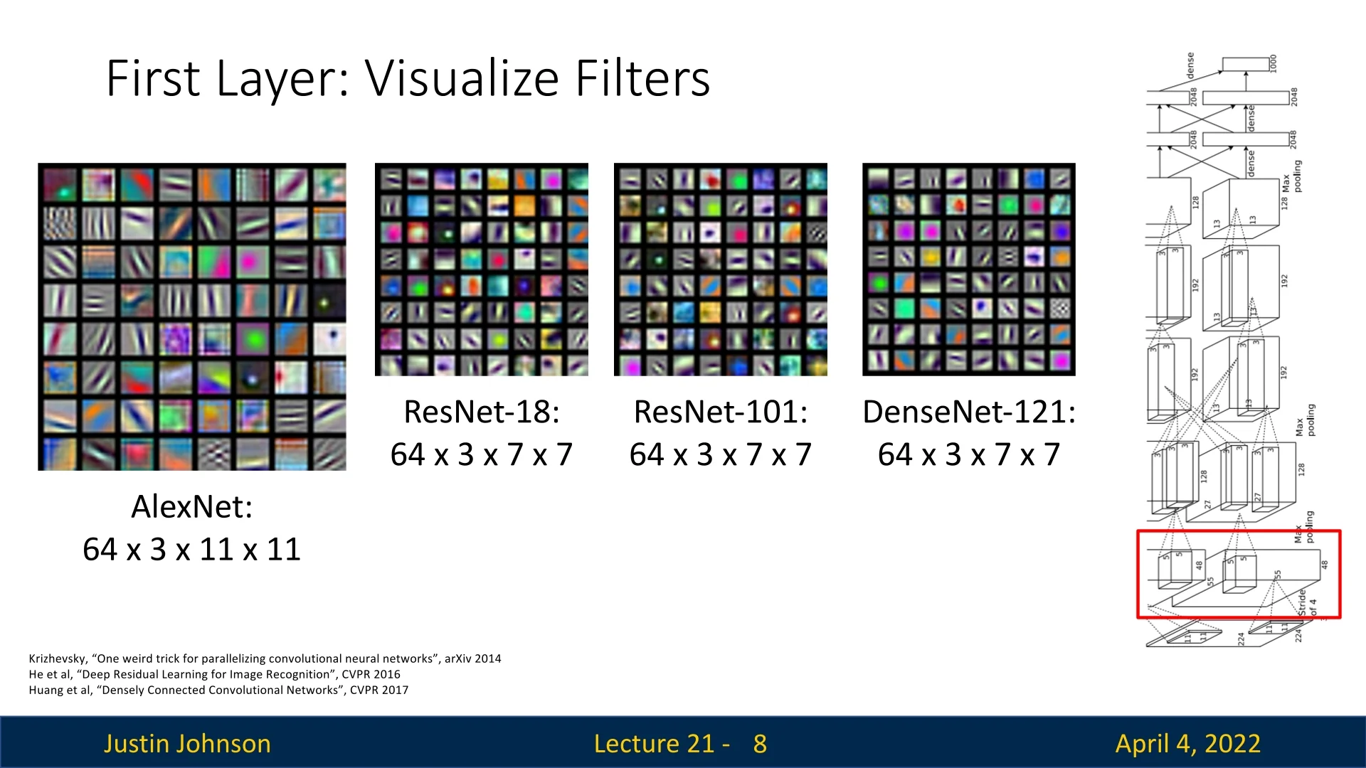
Interpretation and Limitations Because the filters in the first layer operate directly on the input image, they can be visualized straightforwardly as \(K \times K\) RGB patches, with each of the 3 channels contributing to a color composite. This makes the first layer particularly interpretable: we can ”see” what the model is looking for, such as vertical edges, red-green opponency, or high-frequency textures.
However, such visualizations only offer a limited glimpse into the model’s behavior. These filters detect purely local features and do not account for broader spatial context or higher-order semantics. As a result, visualizing the first layer alone provides only shallow insight into the network’s full representational power. To understand how a CNN constructs rich hierarchical features—capable of recognizing objects, parts, and categories—we must investigate deeper layers, where features become increasingly abstract and spatially integrated.
This motivates the exploration of visualization techniques for deeper activations and learned embeddings, which we address in the following sections.
21.1.2 Visualizing Higher Layer Filters
Understanding what deeper layers in a convolutional neural network (CNN) are learning is a central question in interpretability research. While visualizing the first convolutional layer yields intuitive insights—thanks to its direct correspondence with RGB pixel inputs—the situation becomes markedly more complex in deeper layers. These layers no longer respond to simple visual primitives but to abstract feature combinations, making direct visualization of their filters significantly less interpretable.
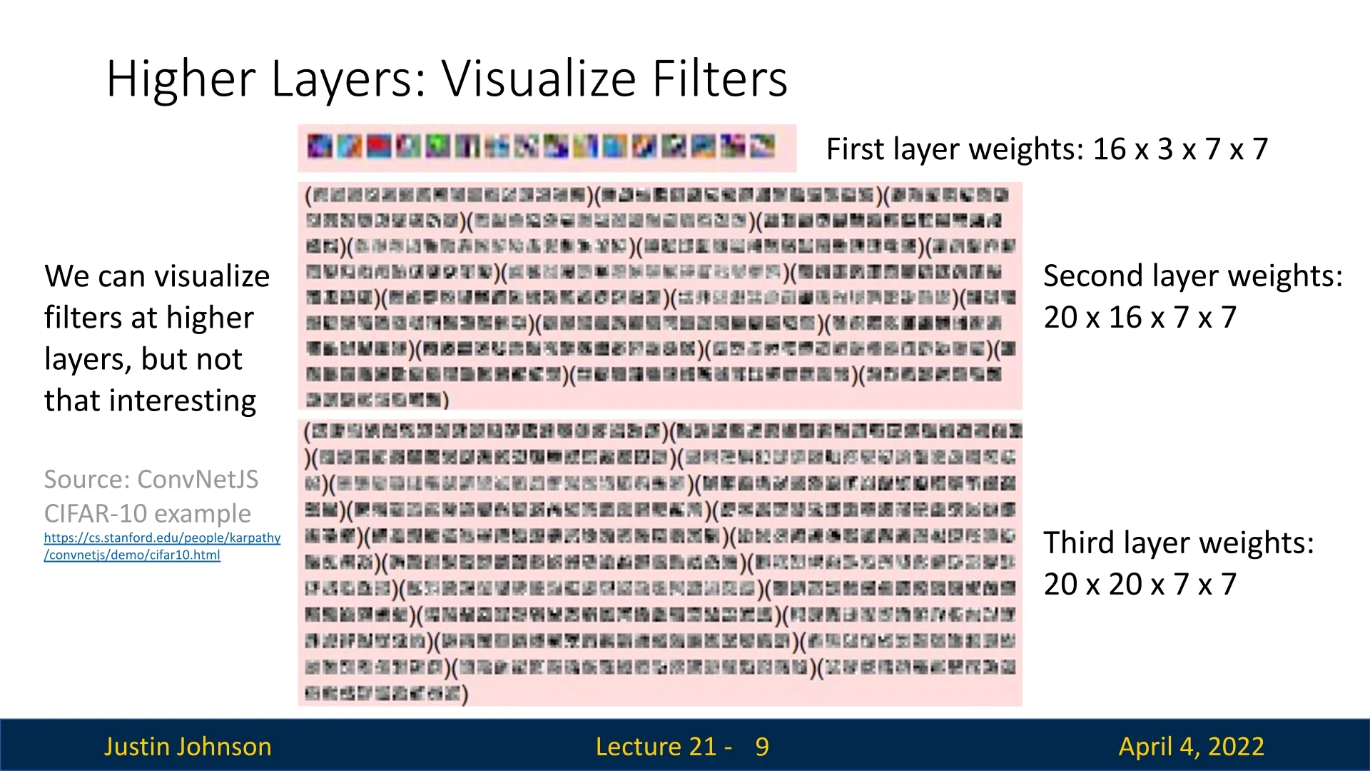
Example: ConvNetJS Visualization To illustrate this challenge, consider a toy CNN trained on CIFAR-10, as implemented in ConvNetJS [11]. The below figure visualizes the raw filter weights from the first three convolutional layers of a simple 3-layer architecture:
- Layer 1: \(16 \times 3 \times 7 \times 7\) — 16 filters applied to 3-channel RGB inputs.
- Layer 2: \(20 \times 16 \times 7 \times 7\) — 20 filters each operating on all 16 feature maps from Layer 2.
- Layer 3: \(20 \times 20 \times 7 \times 7\) — 20 filters applied to the 20 feature maps from Layer 3.
Each filter in deeper layers is a stack of \(K \times K\) slices—one per input channel—which can be visualized as a set of grayscale images. However, as shown in the below figure, while the first-layer filters exhibit recognizable edge and color-selective patterns, the filters from Layers 2 and 3 appear increasingly disorganized and abstract. This reflects a shift in representation: higher-layer filters are no longer tuned to individual pixel-level structures, but to complex combinations of previously learned features.
Interpretation and Motivation for Indirect Methods As we ascend the network hierarchy, each filter becomes sensitive to more intricate spatial compositions—such as repeated textures, curves, object parts, or category-level cues. These higher-order features are not aligned with natural image statistics or directly grounded in the RGB input space. Instead, they are formed by arbitrary nonlinear combinations of earlier-layer activations. Moreover, filters in later layers have larger effective receptive fields, meaning that their responses integrate information across wider regions of the input image.
Consequently, visualizing the raw weights of deeper filters—even as stacks of grayscale slices—fails to reveal their functional role. These weights no longer ”look for” simple patterns, but rather detect abstract configurations of patterns-of-patterns. The lack of spatial or semantic alignment makes their interpretation both difficult and potentially misleading.
To overcome this limitation, later in this chapter we will explore a suite of indirect visualization techniques—such as activation maximization, guided backpropagation, and feature inversion—which help reveal what kinds of inputs actually elicit strong activations in higher-layer units. These methods synthesize or highlight meaningful visual patterns in the input space, offering a more powerful interpretive lens than static filter weights.
Ultimately, this motivates a deeper shift in focus: rather than interpreting filters in isolation, we often care more about the representations that the network constructs—especially at its final convolutional layers. These representations are key to the model’s decision-making process and often contain high-level semantic information. In the following parts, we examine these deep features directly and explore how they encode task-relevant signals.
21.2 Last Layer Features: Nearest Neighbors, Dimensionality Reduction
The final layers of a convolutional neural network (CNN) encode compact, abstract representations that summarize the semantic content of an input image. In classification models such as AlexNet [318], the penultimate fully connected layer—commonly referred to as fc7—produces a 4096-dimensional feature vector. This layer serves as a bottleneck, compressing spatial and visual information into a high-level descriptor that feeds into the final classifier. Understanding these abstract representations is crucial for interpreting model behavior and enables a range of downstream applications beyond classification, including retrieval, clustering, and transfer learning.
21.2.1 Semantic Similarity via Nearest Neighbors
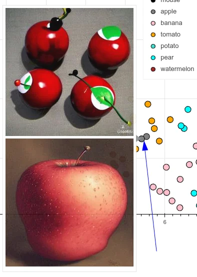
One intuitive technique to probe the quality of learned features is to compute nearest neighbors in the last layer’s (pre SoftMax) feature space. For a given query image, we extract its feature vector from the last layer (pre SoftMax) and compare it to feature vectors from a training set using \(\ell _2\) distance. This produces a ranked list of semantically similar images.
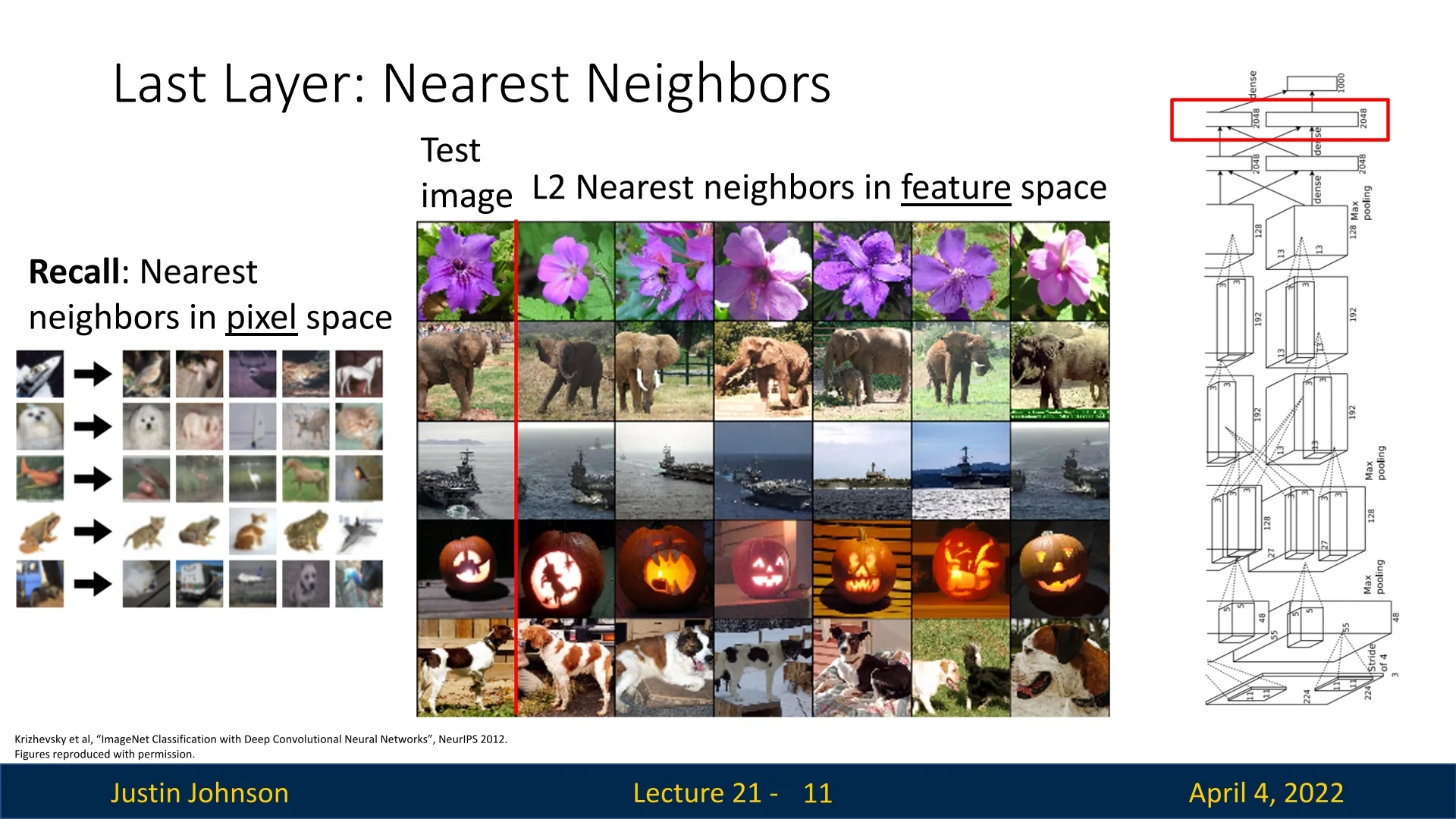
As can be seen in figure 21.3: Unlike raw pixel-space retrieval—which is highly sensitive to low-level variations such as lighting, background, or slight translations—feature-space retrieval captures more robust and semantically meaningful similarities. The features abstract away irrelevant appearance differences and instead emphasize object identity, pose, and scene context. This property makes them especially valuable for applications like image search and dataset exploration.
21.2.2 Dimensionality Reduction and Embedding Visualization
Convolutional neural networks learn to represent images in high-dimensional feature spaces—often with hundreds or thousands of dimensions. While these abstract representations are powerful for classification, similarity, and downstream tasks, they remain difficult to interpret directly. As humans, our intuition and perception are fundamentally limited to low-dimensional spaces like 2D and 3D. To bridge this gap, we turn to dimensionality reduction techniques that project complex feature vectors into interpretable lower-dimensional spaces.
By visualizing these projections, we can uncover how the network organizes inputs: which images cluster together, what semantic properties are preserved, and where decision boundaries might lie. Such visualizations are not only useful for understanding a model’s behavior but also for identifying failure cases, detecting dataset biases, evaluating the quality of artificially generated or augmented data, and exploring representation similarity between tasks.
Two widely used techniques for this purpose are:
-
Principal Component Analysis (PCA): A deterministic, linear projection method that identifies directions of maximum variance in the data. By projecting onto the leading principal components, PCA reduces dimensionality while preserving as much variability as possible. It is particularly effective at capturing global structure and identifying coarse axes of variation such as illumination, scale, or pose. For a practical and intuitive introduction to PCA including Python code and visual demonstrations, we highly recommend Steve Brunton’s excellent video series on Singular Value Decomposition and PCA from the University of Washington.
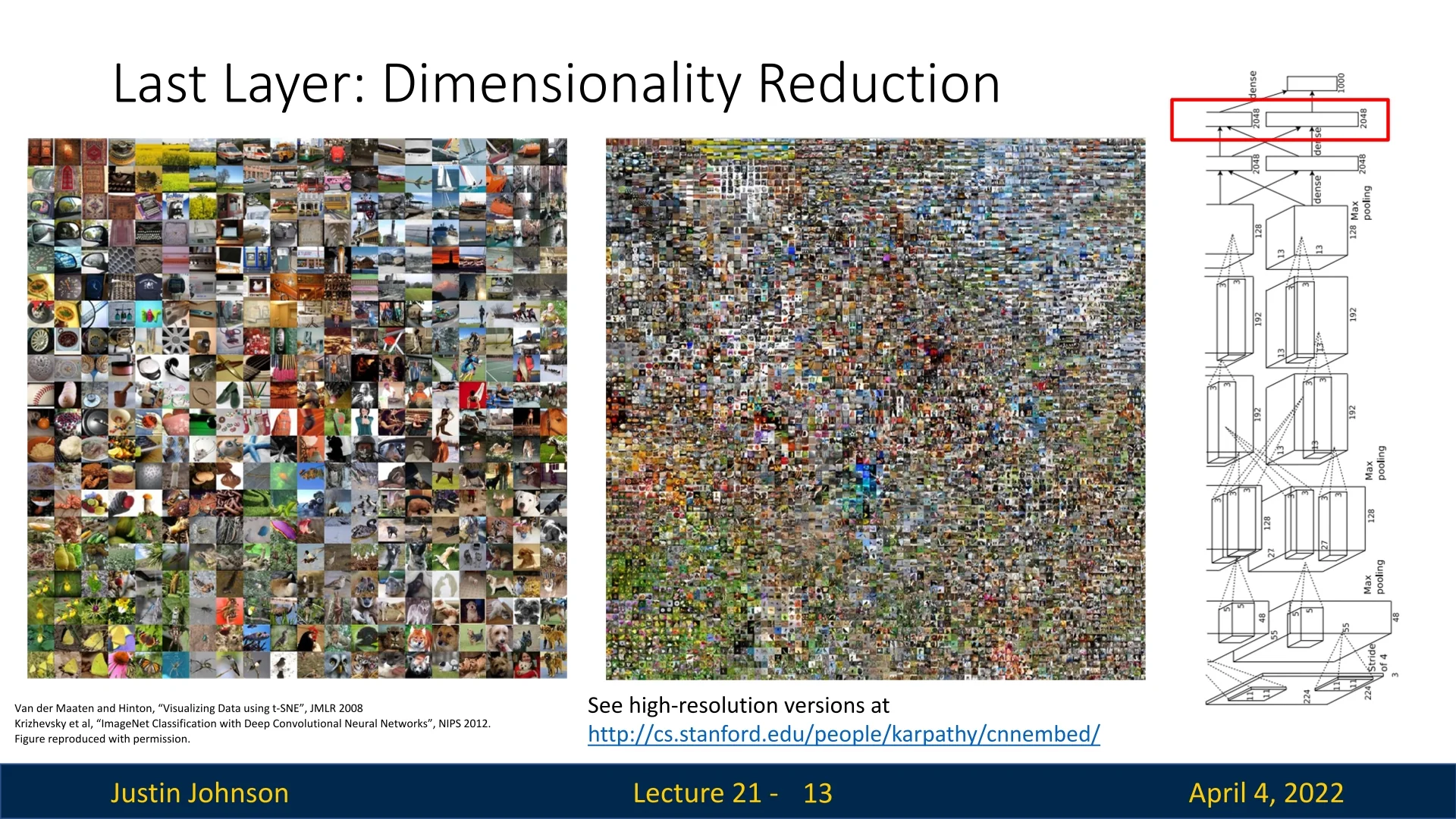
Figure 21.4: A 2D t-SNE visualization of feature vectors extracted from the final FC layer of a CNN trained on ImageNet. Each point represents a test image, positioned such that nearby points in the plot correspond to images with similar features. This nonlinear embedding preserves local neighborhoods, revealing the semantic organization of the learned representation space. For instance, in the bottom left, flower images form a coherent cluster that transitions smoothly into butterflies, illustrating how the network encodes visual similarity. Figure adapted from [422, 318]. - t-Distributed Stochastic Neighbor Embedding (t-SNE): A nonlinear, stochastic technique designed to preserve local structure in the data. Unlike PCA, t-SNE focuses on maintaining neighborhood relationships, often revealing tight semantic clusters that align with object categories, poses, or contextual cues [422]. While t-SNE may distort global distances, it is extremely effective at uncovering fine-grained groupings. For an in-depth and accessible overview of t-SNE’s mechanisms and limitations, see this annotated guide.
While PCA is computationally efficient and preserves global geometry, it often fails to expose local semantic clusters. In contrast, t-SNE is specifically tailored to emphasize local similarities, often revealing latent category structure—but at the cost of distorting distances between distant points and lacking run-to-run consistency. Both methods offer complementary perspectives on the underlying feature space and are often used in tandem for exploratory analysis.
Interpretation and Applications High-level representations such as those from a CNN’s final layers encode rich semantic attributes—ranging from object identity and viewpoint to scene layout and contextual cues. Distances in this feature space often correlate well with human judgments of visual similarity, enabling a wide array of practical applications:
- Image retrieval: Finding visually or semantically similar images in large datasets.
- Dataset visualization: Exploring the structure of labeled or unlabeled image corpora.
- Anomaly detection: Identifying outliers or data points poorly aligned with learned manifolds.
- Unsupervised clustering: Automatically grouping inputs by their learned feature similarity.
- Synthetic data evaluation: Comparing simulated or augmented images to real examples.
Moreover, these high-level embeddings are often transferable: features learned on large classification datasets can be reused in novel tasks or domains with minimal fine-tuning. This principle—central to transfer learning—demonstrates that the representations captured by deep networks are not only powerful, but also generalizable.
In sum, dimensionality reduction provides a crucial bridge between abstract neural representations and human-understandable intuition. Through methods like PCA and t-SNE, we can glimpse how deep models internally organize visual information—and use these insights to refine, audit, and better exploit our models.
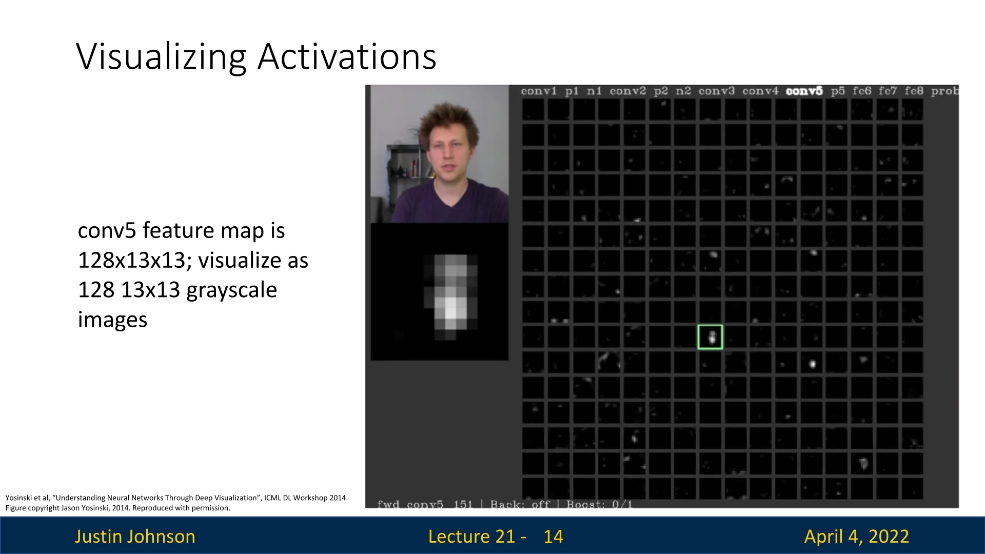
21.3 Visualizing Activations and Maximally Activating Patches
Inspecting the learned weights of a CNN provides a static snapshot of the model’s potential for pattern detection—its architectural “blueprint” for recognizing features. However, to understand what the network actually does when processing a specific input, we often examine its activations—the dynamic feature maps produced as the image flows forward through the network. These activations reveal which filters fire, and crucially, where in the input those activations occur. In this sense, weights describe capacity; activations reveal behavior.
How to Visualize Activations Each convolutional layer produces a 3D tensor of shape \( C \times H \times W \), where:
- \( C \) is the number of filters (channels),
- \( H \times W \) are the spatial dimensions of each activation map.
Each 2D slice \( A_c \in \mathbb {R}^{H \times W} \) reflects how strongly the \( c^\mbox{th} \) filter responds at each spatial location. To visualize a specific activation map:
- 1.
- Select a channel \( c \in \{1, \dots , C\} \) to isolate one filter’s response.
- 2.
- Extract the 2D activation map \( A_c \in \mathbb {R}^{H \times W} \) corresponding to that filter.
- 3.
- Normalize the values to the display range \([0, 255]\), typically via min–max scaling: \[ A'_c = 255 \cdot \frac {A_c - \min (A_c)}{\max (A_c) - \min (A_c)} \] This step is crucial because activations are real-valued and unbounded—some may be small or near-zero (especially due to ReLU), while others are large. Without normalization, these differences would be visually imperceptible.
- 4.
- Render the result as a grayscale image or heatmap. Heatmaps often provide richer visual detail by using color gradients to emphasize intensity differences, making strong responses immediately apparent.
As we move deeper into a convolutional network, filters become increasingly selective—activating only in response to highly specific patterns or abstract visual concepts. Their corresponding activation maps tend to be sparse: most values are zero due to the use of ReLU, which clips all negative responses. Even among nonzero activations, only a few regions typically ”light up.” This sparsity can be beneficial for interpretability, but also poses challenges: min–max normalization of nearly-zero maps can exaggerate noise or suppress subtle, yet semantically meaningful signals. These artifacts must be considered when interpreting visualizations.
Why Do Activation Maps Reveal Spatial Information? Despite their abstract nature, convolutional activations retain spatial structure. Each filter is applied across an input feature map using weight sharing—the same filter is convolved at every spatial position. But the output varies based on the local content in the receptive field at each position. Thus, each activation value \( A_c[h, w] \) reflects how well the filter \( c \) matched the input region centered at position \( (h, w) \).
Visualizing these 2D slices (e.g., a single \(13 \times 13\) map from a \(128 \times 13 \times 13\) tensor) highlights the spatial pattern of a filter’s response. These patterns can be overlaid on the input (via the effective receptive field [417]) to estimate where in the original image the filter was activated. However, deeper layers have increasingly large receptive fields, making it harder to attribute activations to specific image structures. As a result, spatial precision decreases, and interpretability becomes less reliable the further we advance.
What Do Activations Reveal? Activation maps offer a structured way to investigate a CNN’s learned internal representations. Specifically, they let us answer:
- Where (spatial localization): Because convolution preserves spatial arrangement, the activation map shows where in the input each filter fired. This provides coarse localization for the visual features the filter detects, even without class-specific attribution methods.
- What (feature selectivity): By examining the activation maps across many images, we can try to infer the type of feature a filter has learned to recognize. Early layers might detect edges or color gradients [775], while later layers respond to higher-order patterns like textures, object parts, or semantic categories [760, 31].
- When (context sensitivity): Activation strength across varied inputs reveals when a filter activates. Some filters are robust—firing across poses, lighting conditions, or backgrounds—while others activate only under specific circumstances. This sensitivity can indicate generalization strength or overfitting to spurious correlations.
ReLU activation plays a central role in this analysis: it promotes sparsity, simplifying interpretation by highlighting only strong, positive responses. But it also discards all negative values—even those with large magnitude—thereby removing potentially informative inhibitory signals. To recover this information, one may inspect pre-ReLU activations or experiment with nonzero-centered alternatives such as Leaky ReLU or ELU [111]. The trade-off between sparsity and representational richness remains an open research question.
What Can We Do With Activation Maps? Beyond visual intuition, activation maps support quantitative analysis and practical improvements:
- Debug unexpected behavior and expose spurious correlations: If a filter activates consistently in irrelevant regions—e.g., sky, grass, or watermarks—it may signal that the model relies on background cues rather than object-relevant features. For instance, a ”cow” detector firing primarily on grass may indicate dataset bias.
- Evaluate feature generality and specialization: By comparing activation maps across inputs, we can assess whether filters detect broad, reusable patterns (e.g., wheels across vehicle types) or overfit to narrow visual contexts (e.g., specific breeds or lighting). This aids in diagnosing underfitting, overfitting, or insufficient dataset diversity.
-
Guide architectural and training improvements:
- Pruning: Filters that remain inactive across most inputs may be redundant and removable.
- Augmentation: Overly selective filters may indicate a need for targeted data augmentation (e.g., varied viewpoints or occlusions).
- Architecture tuning: Imbalanced usage of filters across layers may suggest overparameterization or motivate the use of attention, bottlenecks, or depth adjustments.
However, it’s important to recognize the limits of activation map interpretability, leading us towards further research and hopefully better approaches. We remind the reader that in deeper layers, features become more abstract and distributed, and receptive fields cover large, overlapping regions of the input. As a result, the exact visual trigger for a given activation may no longer be clearly localized. While activation maps remain a powerful tool—especially for understanding early and mid-level representations—their utility diminishes in deeper layers, where methods like class activation mapping (CAM) or feature inversion that we’ll cover later become more appropriate.
21.3.1 Maximally Activating Patches
To gain a more concrete and intuitive understanding of what a convolutional filter has learned, an effective strategy is to examine the image regions that elicit the strongest responses from that filter. This technique, known as the maximally activating patch method, identifies the specific visual patterns that most excite a given channel or neuron across a diverse dataset. Rather than inspecting weights or abstract feature maps, we directly observe which natural image patches consistently trigger high activations—revealing the visual motifs the network has internalized.
Methodology The process consists of the following steps:
- 1.
- Select a target filter: Choose a specific convolutional layer and channel (e.g., channel 17 in conv5). This channel acts as a spatially replicated detector for a particular feature across the input.
- 2.
- Forward a dataset through the network: Pass a large collection of diverse images through the network. For each image, record the full spatial activation map of the selected channel—i.e., all values \( A_c[h, w] \) at every spatial location.
- 3.
- Aggregate and rank responses: Collect all activation values from all images and spatial positions. Identify the top-K strongest activations globally—these are the spatial locations and images where the filter responded most strongly across the dataset.
- 4.
- Extract corresponding patches: For each of these peak activations, compute the receptive field in the original input image that led to the activation. This mapping depends on the layer’s position in the network (e.g., kernel size, stride, padding, pooling). Extract that region from the input—this is the maximally activating patch for the neuron.
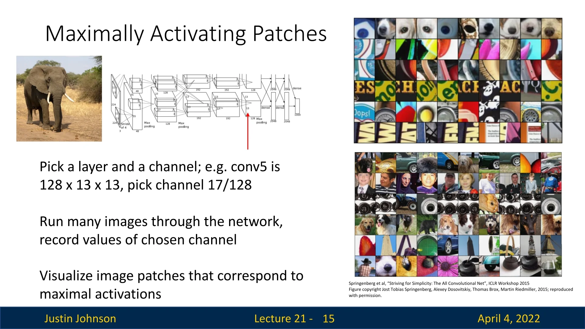
This method is most directly interpretable in fully convolutional architectures, where each spatial location in an activation map corresponds to a fixed receptive field in the input image. The spatial correspondence in CNNs enables straightforward mapping from filter activations back to the regions of the input that caused them. While exact pixel-level alignment can be imprecise—due to overlapping receptive fields, nonlinear activations, pooling layers, and stride effects—the extracted patches still reliably capture the dominant local visual stimulus that triggered the filter’s response. As such, they offer a concrete and intuitive glimpse into what the neuron has learned to detect.
Intuition and Insights This method gives us a dataset-level understanding of what a neuron ”looks for”. By observing many input patches that excite a filter, we can infer its role in the learned feature hierarchy. For example, some neurons specialize in detecting:
- Low-level cues like diagonal edges or color gradients.
- Mid-level textures such as mesh, fur, or bricks.
- High-level semantics such as eyes, animal faces, or wheels.
These patterns tend to be consistent across inputs, offering a clear visual prototype of the features the filter has internalized.
Beyond interpretability, this method supports diagnosis:
- Redundancy: If many neurons are activated by visually similar patches, it may suggest overparameterization and motivate pruning.
- Dataset bias: If a neuron fires only when a feature appears in a specific context (e.g., a texture always on green grass), it may indicate reliance on spurious correlations in the training data.
From “What It Sees” to “What It Uses” Taken together, activation maps and maximally activating patches provide complementary perspectives on the behavior of individual filters in a convolutional neural network:
- Activation maps show where in a specific input image a filter activates. They highlight the spatial regions that match the filter’s learned pattern in that image, offering localized insight into the filter’s response.
- Maximally activating patches reveal what the filter is most tuned to detect. By scanning across many inputs and extracting only the input regions that trigger the strongest responses, this method uncovers the most prototypical visual stimuli associated with that filter—regardless of their spatial position.
While activation maps offer per-image spatial footprints, maximally activating patches distill a filter’s dataset-wide preferences. The former tells us where a filter fires; the latter tells us what consistently causes it to fire.
However, both techniques are inherently class-agnostic. They tell us which features a filter responds to and where it detects them—but not whether those responses contribute positively, negatively, or at all to the model’s final decision for a specific class. In other words, they capture what the network notices, but not what it relies on to make a prediction.
To move from feature visualization to decision attribution, we need methods that explicitly measure how changes to specific input regions affect the output logits or class probabilities. This brings us to the domain of saliency methods—a family of techniques designed to reveal which parts of the input were most influential in producing a particular output. We begin this journey with one of the most direct and interpretable approaches: saliency via occlusion.
21.4 Saliency via Occlusion and Backpropagation
Saliency methods aim to identify which parts of an input image are most influential for a model’s prediction. These techniques produce spatial or pixel-level explanations by quantifying how sensitive the model’s output is to perturbations in the input—highlighting the regions that contribute most strongly to the predicted class.
21.4.1 Occlusion Sensitivity
A natural way to probe a model’s decision is to ask: “What happens if we hide part of the input?” Occlusion sensitivity [775] follows this idea in a simple, model-agnostic manner. It systematically occludes small patches of the input image—one at a time—and measures how the predicted class confidence changes. If masking a region leads to a significant drop in confidence, that region likely contains features critical to the model’s decision.
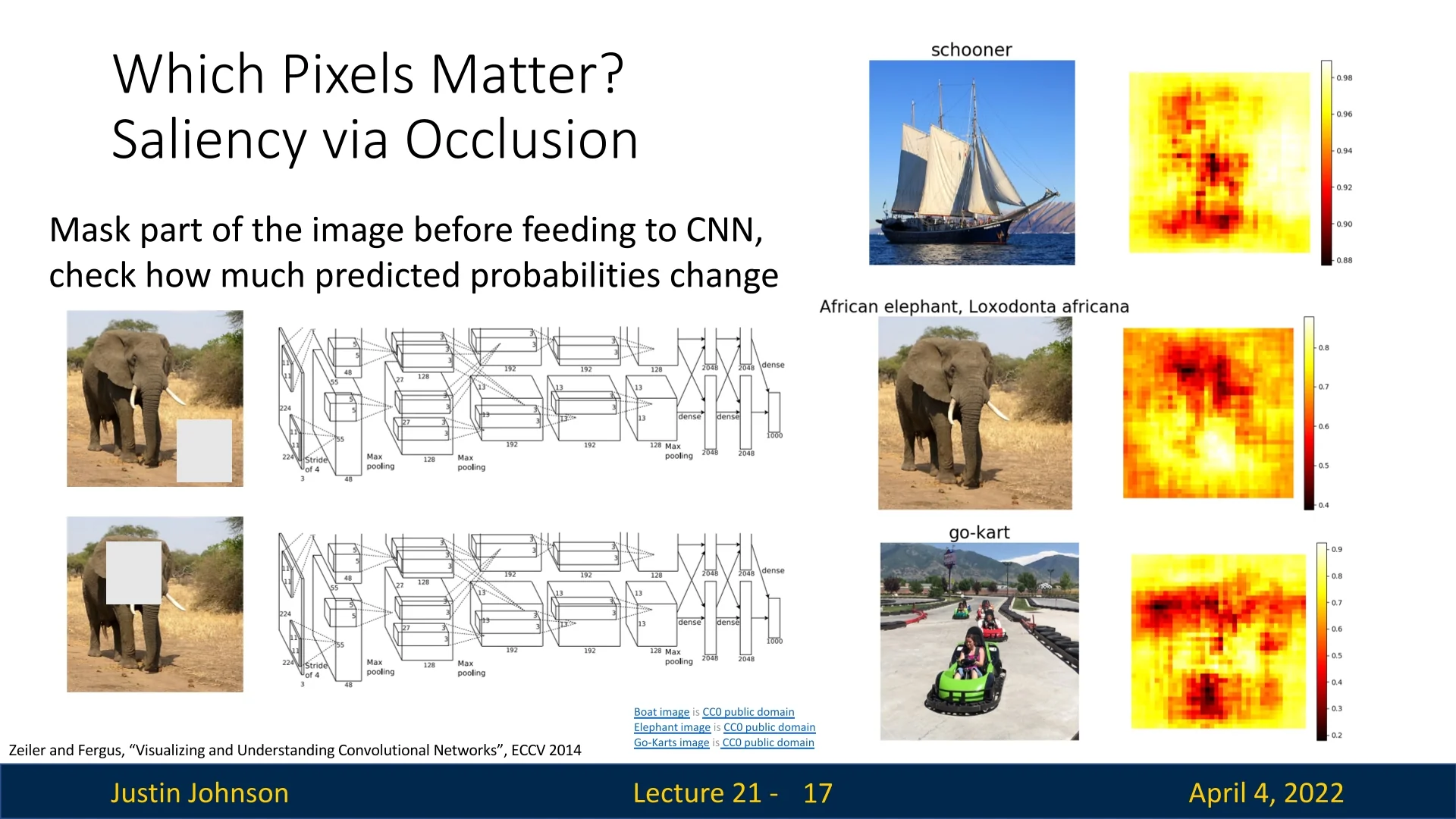
- 1.
- Define occlusion patches: Subdivide the input image into a grid of fixed-size patches (e.g., \(15 \times 15\) pixels), optionally using stride \(s\) to control overlap.
- 2.
- Mask one patch at a time: Replace each patch with a neutral baseline—commonly a gray square, blurred patch, or zero-valued block—to simulate information removal.
- 3.
- Measure impact on prediction: For each occluded image, run a forward pass through the model and compute the change in the predicted confidence score for the target class. The larger the drop, the more critical the masked region is assumed to be.
From Patch Scores to Pixel-Level Saliency This process yields a grid of scalar values, each representing the change in confidence caused by occluding a particular patch. To convert this into a smooth, pixel-level saliency map:
- Assign each patch’s score to the pixels it covered—either uniformly or centered.
- If patches overlap, aggregate the contributions to each pixel by summing or averaging over all occlusions affecting that location.
- Interpolate the resulting low-resolution grid to match the full image resolution, optionally applying smoothing to reduce blocky artifacts.
The result is a dense saliency map that visually highlights which regions of the input the model relied on most for its prediction. Note that in many visualizations, darker areas indicate stronger drops in confidence—i.e., occlusions that had the most damaging effect on classification. These regions are interpreted as the most influential for the model’s decision.
Intuition and Interpretation Occlusion sensitivity provides a direct, human-interpretable diagnostic: “If I hide this part of the input, does the model still know what it’s looking at?” By observing how the model’s confidence changes in response to occlusions, we infer which parts of the input are functionally necessary for the current prediction. Unlike gradient-based saliency, this technique does not rely on access to internal parameters or derivatives—it simply perturbs the input and watches how the output responds.
Enrichment 21.4.1.1: Advantages and Limitations of Occlusion Sensitivity
Advantages:
- Model-agnostic: Requires no access to model weights or gradients. Works with any black-box model.
- Conceptually intuitive: Its interpretation is straightforward and visual—important regions are those whose absence hurts confidence.
- Localized insight: Provides evidence tied to specific input regions, often yielding interpretable and faithful attributions.
Limitations:
- Computational cost: Requires one forward pass per patch. For high-resolution images or small stride, this becomes expensive.
- Resolution trade-off: Smaller patches improve spatial granularity but increase the number of required evaluations.
- Out-of-distribution masking: Large or abrupt occlusions may produce unrealistic inputs, potentially confusing the model.
- Mask design bias: The choice of occlusion value (e.g., gray vs. blur vs. noise) can significantly affect results.
21.4.2 Saliency via Gradient Backpropagation
A more efficient method is to compute the gradient of the output score with respect to the input pixels [590]. This produces a saliency map where each pixel’s intensity corresponds to the magnitude of its influence: \[ M_{i,j} = \max _{c \in \{R,G,B\}} \left | \frac {\partial S_y}{\partial I_{i,j,c}} \right | \] Here, \(S_y\) is the unnormalized score for the predicted class \(y\), and \(I_{i,j,c}\) is the pixel value at location \((i,j)\) and channel \(c\). The result is a single-channel map that highlights pixels with the highest influence on the model’s decision.
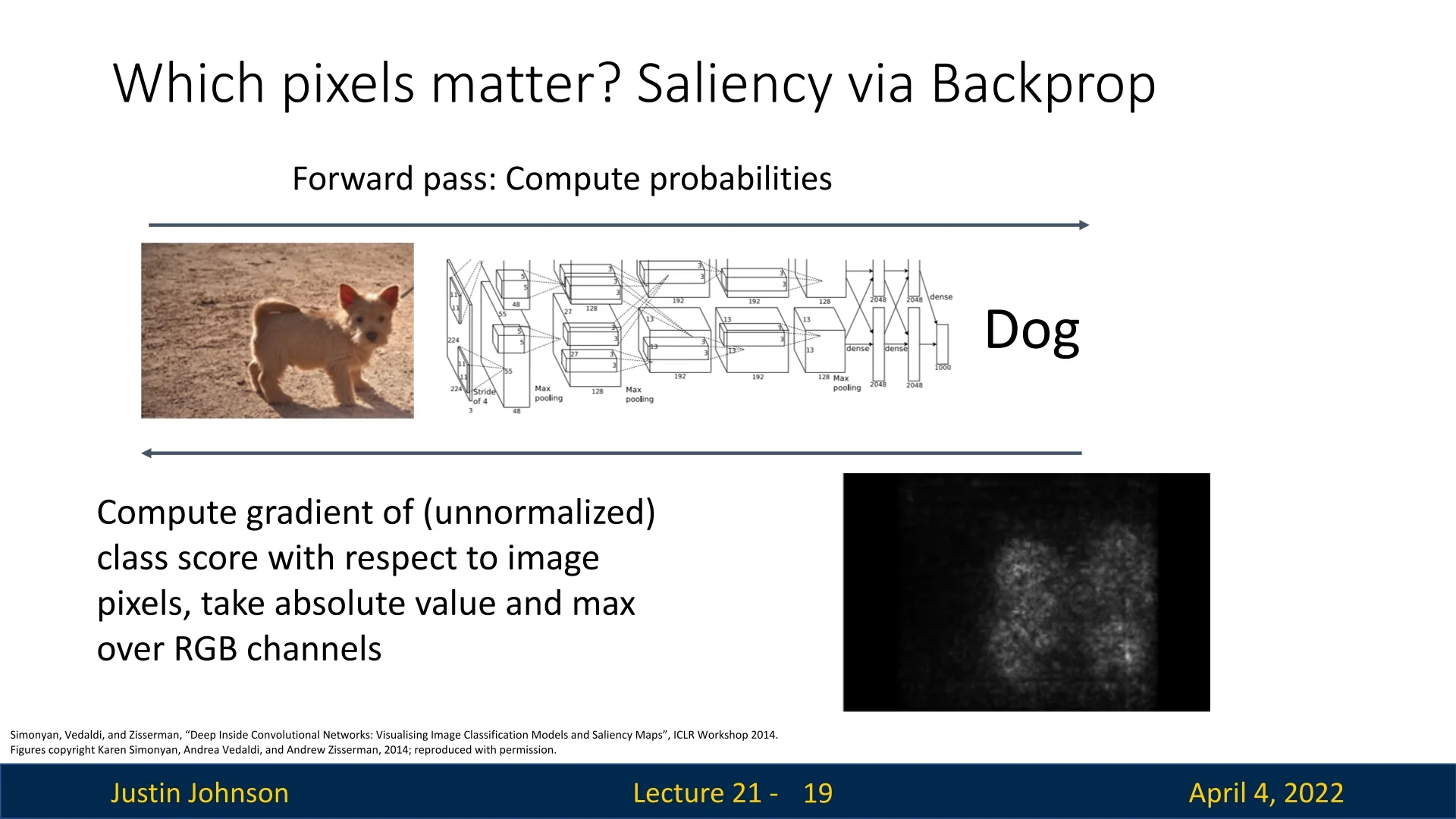
Interpretation and Use Cases Gradient-based saliency maps are useful for:
- Localizing object evidence: Which pixels most support the class prediction?
- Debugging dataset bias: Are predictions based on background cues or spurious features?
- Comparing models: How do different architectures attend to input?
Despite their appeal, gradient saliency maps can be noisy and sensitive to model initialization and ReLU saturation.
Towards Unsupervised Segmentation
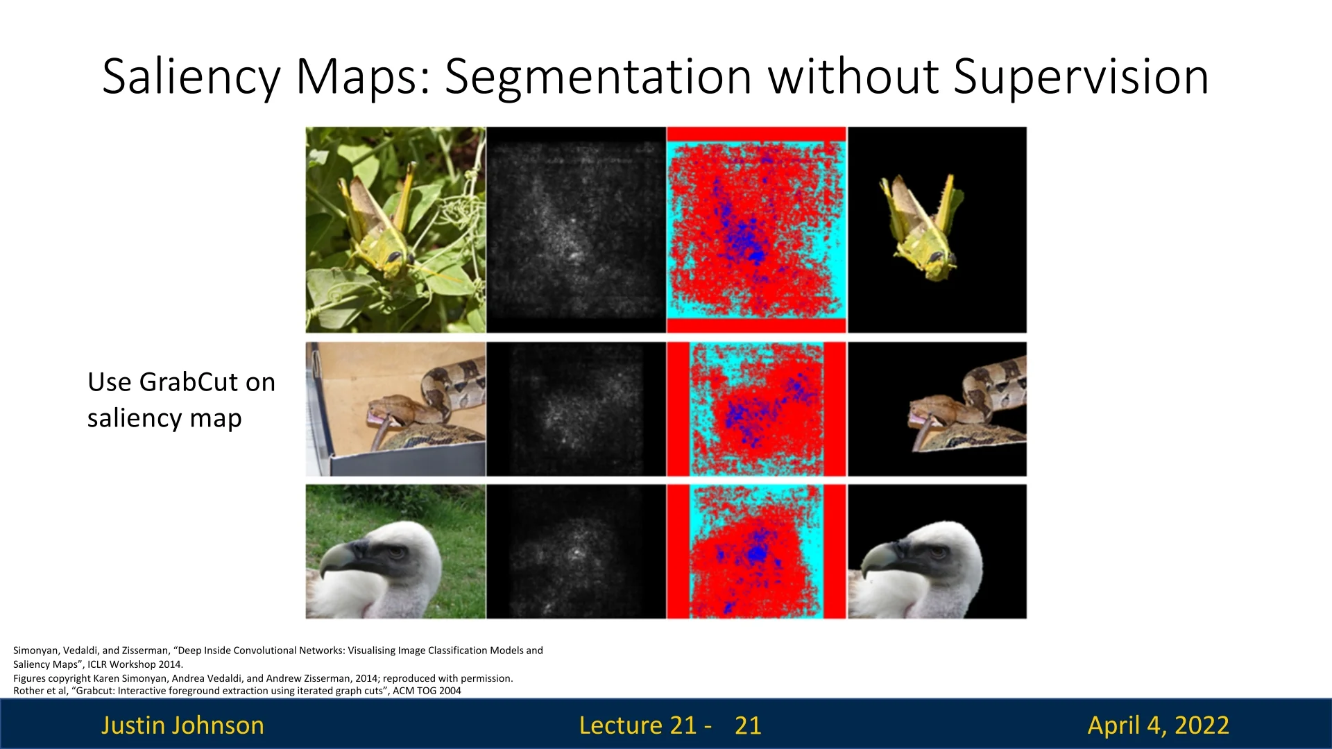
As illustrated in Figure 21.10, Simonyan et al. [590] demonstrated that applying classical segmentation algorithms such as GrabCut [552] to gradient-based saliency maps can yield surprisingly accurate foreground-background separation—even though the network was trained solely for classification. This finding underscores the spatial coherence of CNN attention: regions that most influence class predictions often align well with object boundaries.
While these examples are often cherry-picked and performance may vary considerably across diverse images and classes, the result is nonetheless striking. It suggests that high-level classification networks can implicitly acquire useful spatial priors, hinting at their potential for weakly supervised or unsupervised segmentation—without access to any ground-truth masks.
21.5 Guided Backpropagation of Intermediate Features
Gradients are typically used to update model weights during training—but they can also be repurposed for interpretability. While basic saliency maps compute the gradient of the class score with respect to input pixels, here we extend that idea: instead of analyzing the output neuron, we ask what causes a specific intermediate neuron to activate. This allows us to inspect what internal features a CNN is detecting at various depths.
21.5.1 Backpropagation to Visualize Intermediate Neurons
Given an input image, we forward it through the network and pause at an intermediate convolutional layer (e.g., conv5). This layer outputs a tensor of shape \( C \times H \times W \)—where \( C \) is the number of channels (filters), and \( H \times W \) is the spatial resolution. We select a specific neuron, defined by its channel index \( c \) and spatial location \( (h, w) \), and compute the gradient of that neuron’s activation with respect to the input image:
\[ \frac {\partial A_{c, h, w}}{\partial I} \]
This tells us which pixels in the input image most strongly influence the activation of that individual neuron. Intuitively, it shows the pattern the neuron is ”looking for”—that is, what input changes would most affect that neuron’s response.
Visualizing raw gradients of the class score with respect to input pixels often yields noisy and unintelligible maps. This noise arises primarily from how gradients propagate through nonlinear activation functions like ReLU. In particular, irrelevant negative signals can be amplified or useful contributions canceled, obscuring the underlying patterns that truly drive the model’s decision.
21.5.2 Guided Backpropagation: Cleaner Gradient Visualizations
To address this issue, guided backpropagation [606] modifies the backward pass through ReLU layers to suppress uninformative gradients and emphasize relevant, excitatory input patterns. It introduces an additional masking rule during backpropagation:
- Forward pass: ReLU behaves as usual, blocking all negative activations: \( f(x) = \max (0, x) \).
- Standard backward pass: Gradients are blocked if the forward activation was non-positive. That is, if \( x \le 0 \), then \( \frac {\partial L}{\partial x} = 0 \).
- Guided backpropagation backward pass: Gradients are blocked unless both the forward activation \( x \) and the backward gradient \( \frac {\partial L}{\partial y} \) are positive. This can be expressed as: \[ \frac {\partial L}{\partial x} = \begin {cases} \frac {\partial L}{\partial y} & \mbox{if } x > 0 \mbox{ and } \frac {\partial L}{\partial y} > 0 \\ 0 & \mbox{otherwise} \end {cases} \]
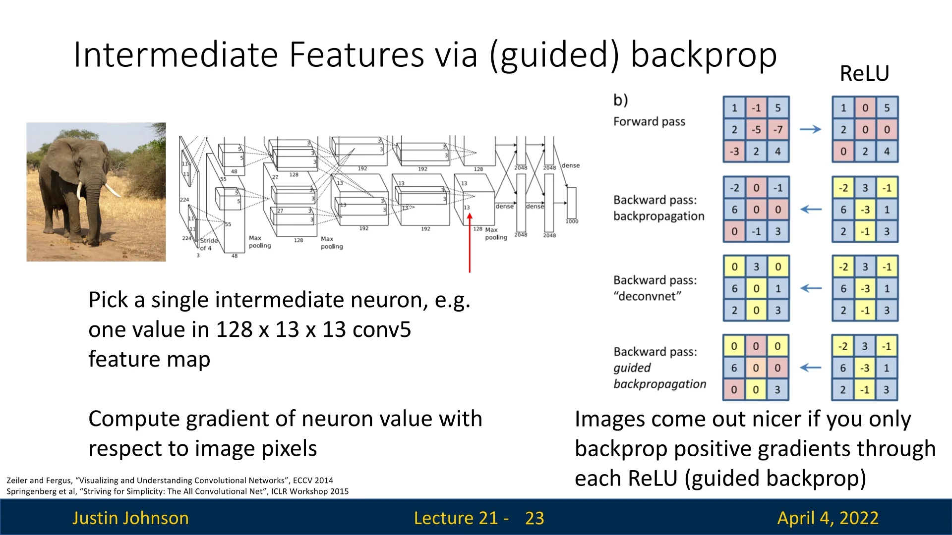
Why Does This Help? Intuition and Impact The exact reasons remain somewhat speculative. What we can empirically deduce is that guided backpropagation appears to suppress noisy or ambiguous gradient signals—particularly those that inhibit neuron activation. By allowing only positive gradients to flow through positively activated neurons, it emphasizes features that excite the network, positively supporting the prediction, filtering out suppressive or indirect influences.
21.5.3 Visualizing Intermediate Feature Detectors
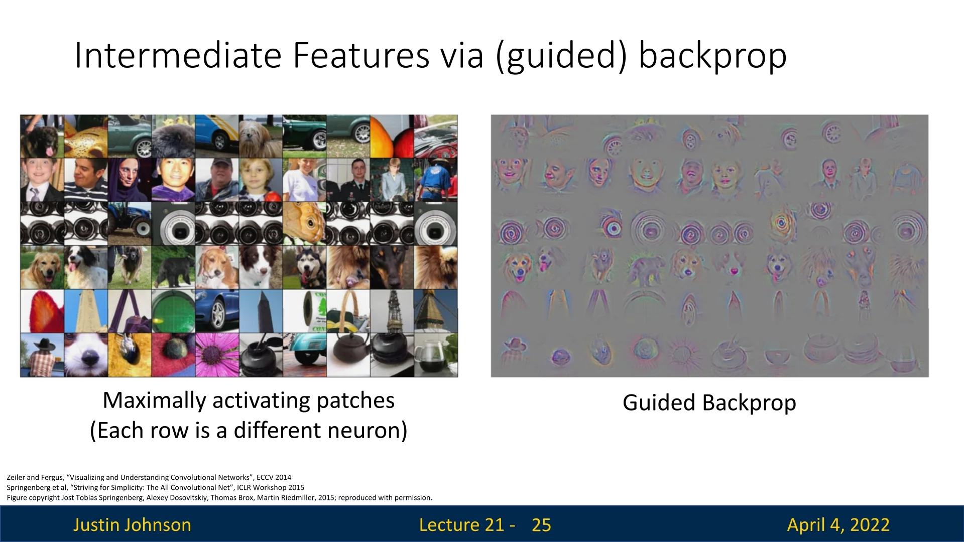
Guided backpropagation enables us to generate clear and interpretable visualizations of what each intermediate neuron responds to. For a given neuron and image, the resulting gradient map highlights which pixels in that input most strongly support that neuron’s activation.
This technique complements the maximally activating patch method ( 21.3):
- Maximal patches show what kinds of image regions trigger a neuron across the dataset.
- Guided backpropagation shows which pixels within a specific image were responsible for that neuron’s response.
Together, they offer both a global and local perspective on what each neuron represents: global preferences from real data, and fine-grained pixel attributions within those preferred regions.
From Saliency to Synthesis So far, our methods have analyzed fixed input images—identifying which parts contributed most to a class prediction or neuron activation. But we can ask a more ambitious question: What image—real or synthetic—would maximally activate a given neuron? Instead of attributing importance within a fixed input, we aim to generate an image from scratch that embodies the neuron’s ideal stimulus. This leads to the next technique: gradient ascent visualization, where we synthesize images by directly optimizing the input to activate specific neurons.
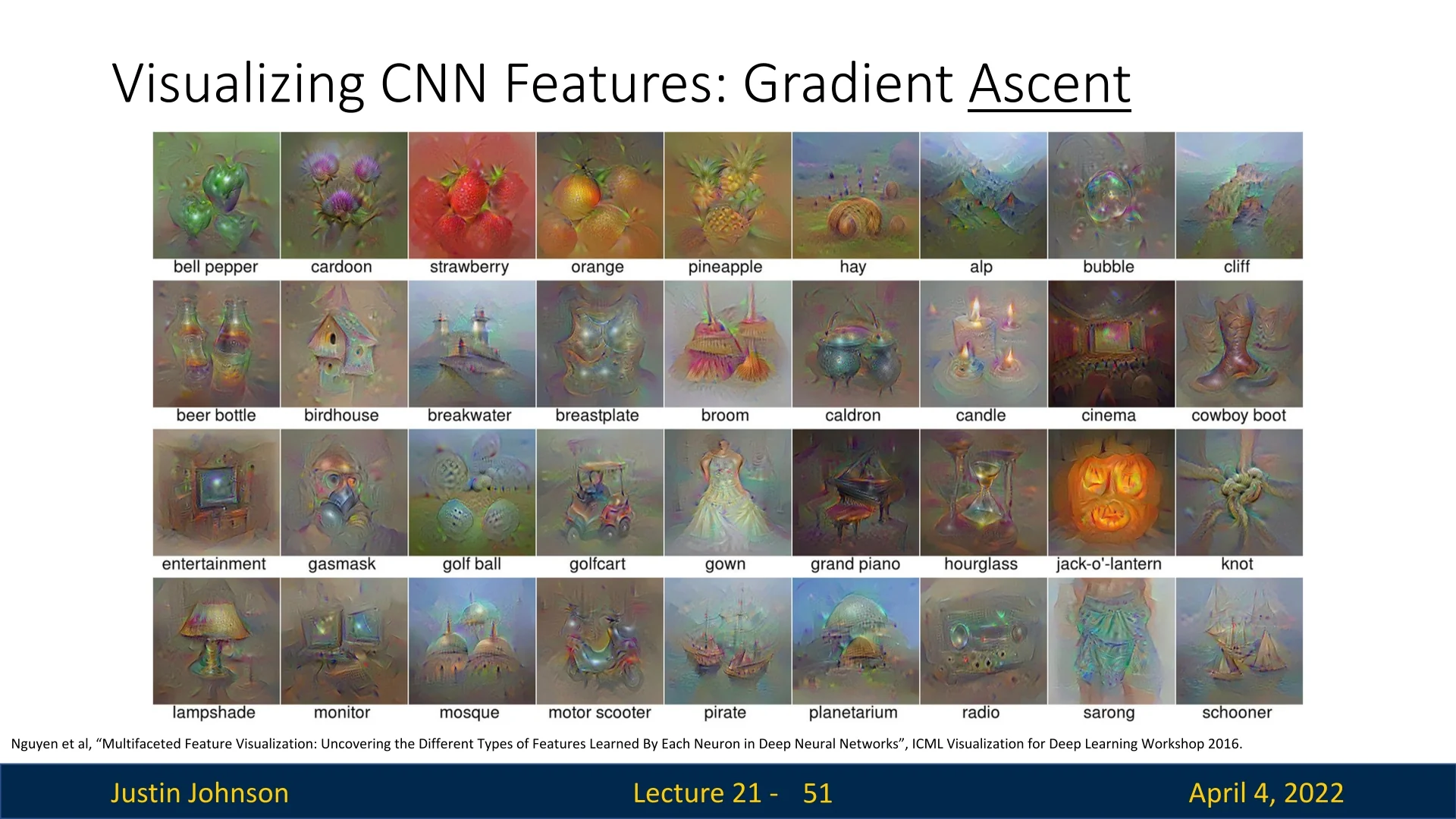
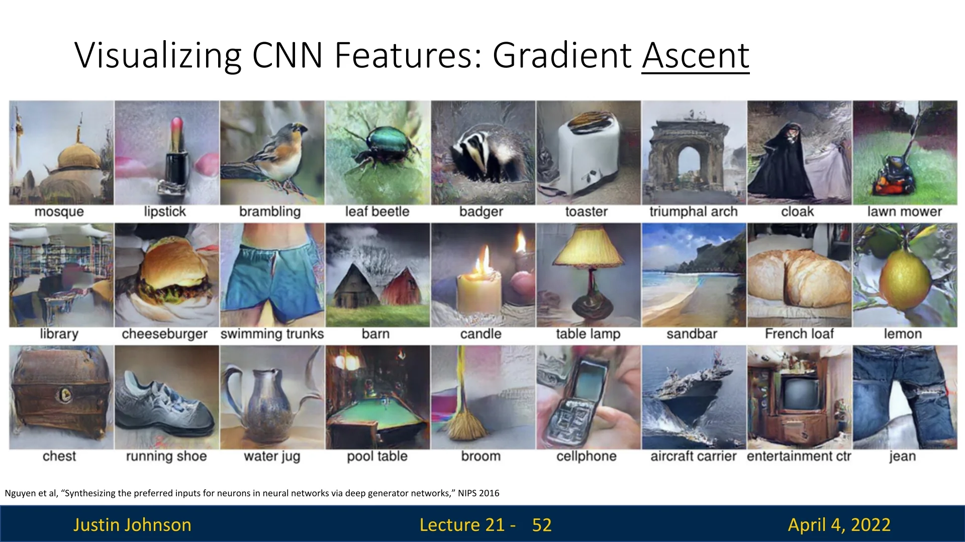
21.6 Gradient Ascent and Class Visualization
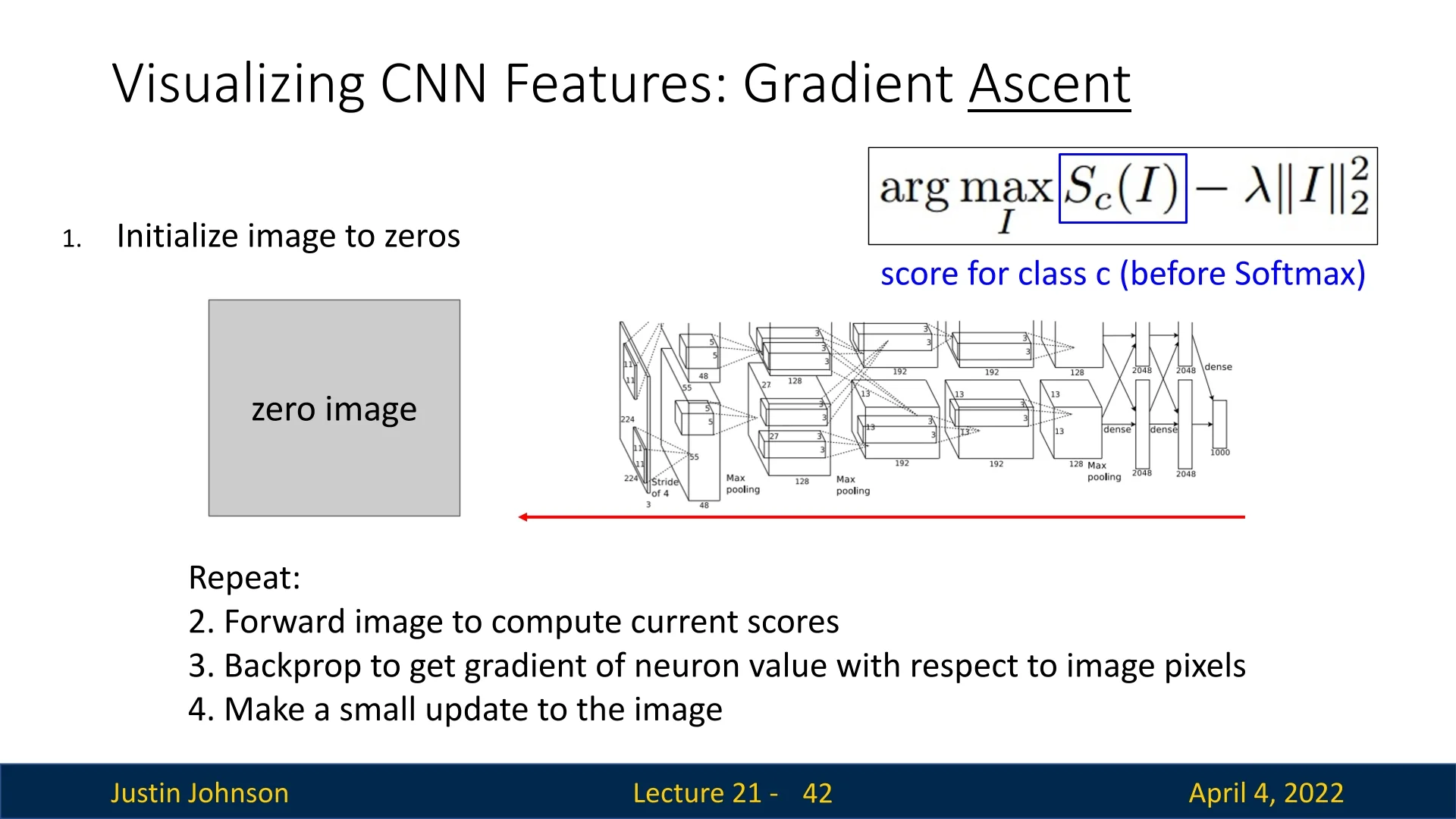
Instead of inspecting how a fixed image influences a network’s prediction, we now flip the process: we synthesize an input image that maximally activates a specific neuron. This neuron can reside in the final classification layer or any intermediate feature map. The network is treated as a frozen function \(f(I)\) with respect to input image \(I\), and our goal is to optimize the image itself.
Objective Function Formally, we wish to find an image \(I^{\ast }\) that maximizes a scalar objective function \(f(I)\)—for example, the activation of a specific neuron—while also maintaining visual plausibility: \[ I^{\ast } = \arg \max _{I} \underbrace {f(I)}_{\mbox{neuron activation}} + \underbrace {R(I)}_{\mbox{image prior regularization}} \] Here:
- \(f(I)\) is the value of the neuron we wish to maximize.
- \(R(I)\) is a regularization term that encourages the image to resemble a natural input.
Optimization via Gradient Ascent To optimize this objective, we perform gradient ascent directly on the image:
- 1.
- Initialize \(I \leftarrow 0\) (e.g., a zero image).
- 2.
- Forward propagate \(I\) through the network to compute \(f(I)\).
- 3.
- Backpropagate \(\partial f(I)/\partial I\) to obtain gradients w.r.t. the input pixels.
- 4.
- Update the image: \(I \leftarrow I + \eta \cdot \nabla _I \left ( f(I) + R(I) \right )\)
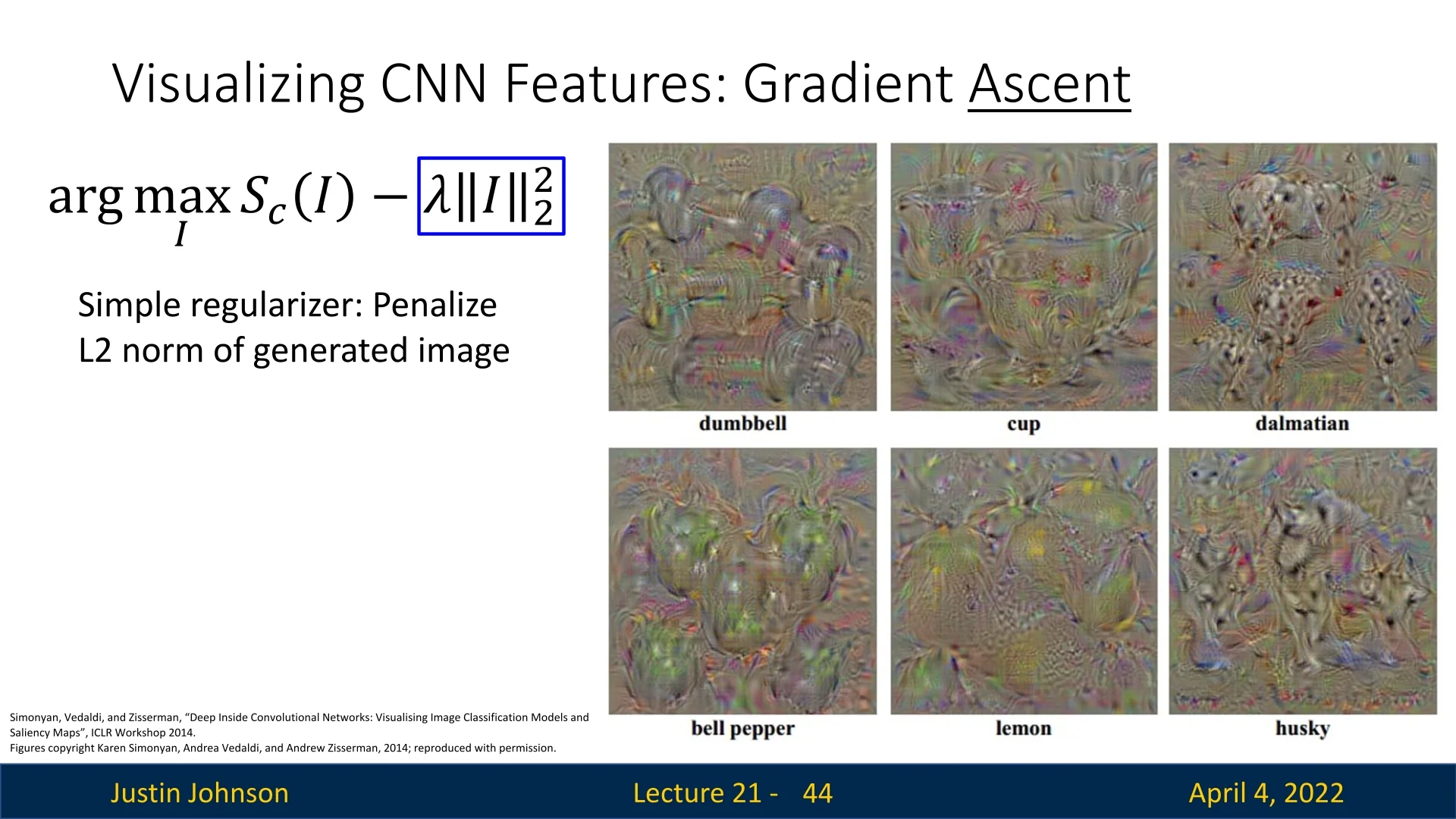
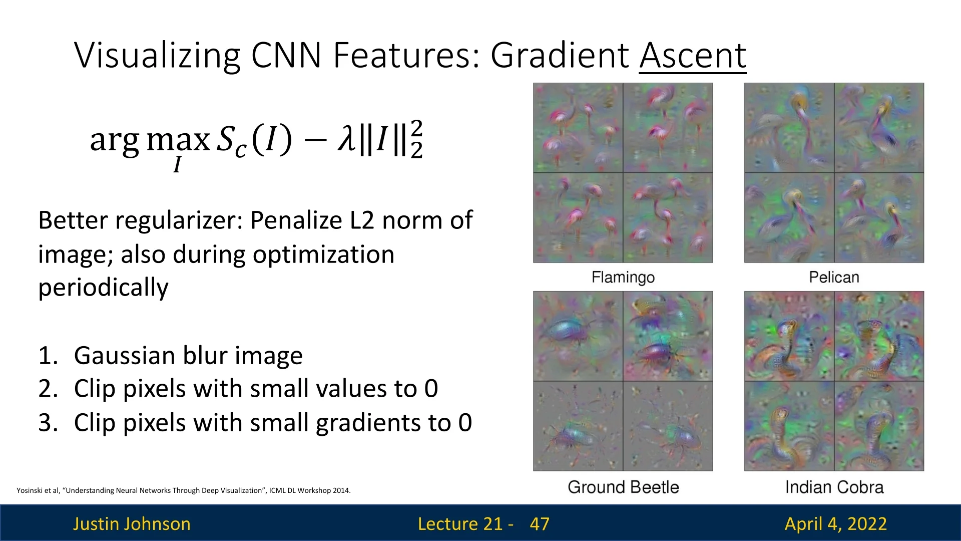
21.6.1 Regularization: Making Images Look Natural
Without regularization, the optimization typically yields noisy, high-frequency artifacts. A simple baseline is \(\ell _2\)-norm regularization [590]: \[ R(I) = -\lambda \|I\|_2^2 \] This penalizes pixel magnitudes and encourages smoother patterns.
Advanced Regularizers We can improve image realism by applying additional constraints:
- Apply Gaussian blur during optimization.
- Set small pixel values to zero (hard-thresholding).
- Set small gradients to zero (gradient masking).
These enhancements reduce noise and amplify dominant structures in the image, as shown in the below figure.
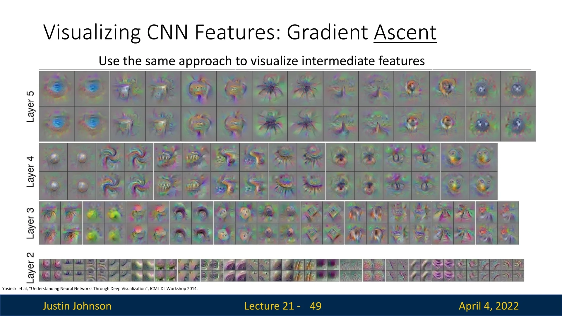
21.6.2 Visualizing Intermediate Features
We can apply the same gradient ascent technique to neurons inside hidden layers. By optimizing \(f(I)\) for a specific feature map location in a middle layer (e.g., conv3 or conv5), we uncover abstract texture patterns that these filters specialize in.
Multifaceted Feature Visualization via Generative Models
Earlier methods synthesized preferred inputs using direct gradient ascent in image space, often constrained by simple regularizers like \(\ell _2\). While interpretable to some degree, these visualizations tended to be noisy and unnatural. To generate more realistic and semantically coherent preferred inputs, Nguyen et al. [461] proposed optimizing within the latent space of a deep generative model—such as a GAN or autoencoder—pretrained to produce natural images.
By searching for latent vectors that produce images which maximally activate a given neuron, this approach yields high-quality visualizations that stay within the data distribution. Crucially, it also enables multifaceted analysis: neurons often respond to several distinct visual modes, and these can be surfaced by clustering the top activating examples and synthesizing a prototype for each cluster.
Realism vs. Fidelity While generative models produce more interpretable and visually compelling results, they also introduce a strong prior that can bias the outcome. The visualizations may reflect assumptions encoded in the generator rather than the raw, unregularized preferences of the target neuron. Simpler methods—such as direct optimization in pixel space with basic regularizers—may yield less realistic but more faithful views into the network’s internal objectives. This reflects a fundamental trade-off between interpretability and fidelity in feature visualization.
21.7 Adversarial Examples: A Deep Dive into Model Vulnerability
Adversarial examples are inputs containing subtle, human-imperceptible perturbations that cause deep neural networks to misclassify with high confidence. This phenomenon reveals a profound vulnerability in the robustness of state-of-the-art AI models, with critical implications for security-sensitive and safety-critical domains such as autonomous driving, medical diagnostics, and facial recognition.
21.7.1 Fundamental Attack Mechanisms
From a technical perspective, the crafting of adversarial examples closely mirrors the gradient-based input optimization techniques introduced earlier for model interpretation—such as saliency maps and preferred input synthesis. However, while those techniques maximize the activation of a given class to better understand what the model has learned, adversarial attacks use the same machinery to intentionally fool the model.
The generation of an adversarial input typically involves solving an optimization problem to find a minimally perturbed version \( I^{\ast } \) of a given input \( I_{\mbox{orig}} \) that causes the model to output an incorrect class label.
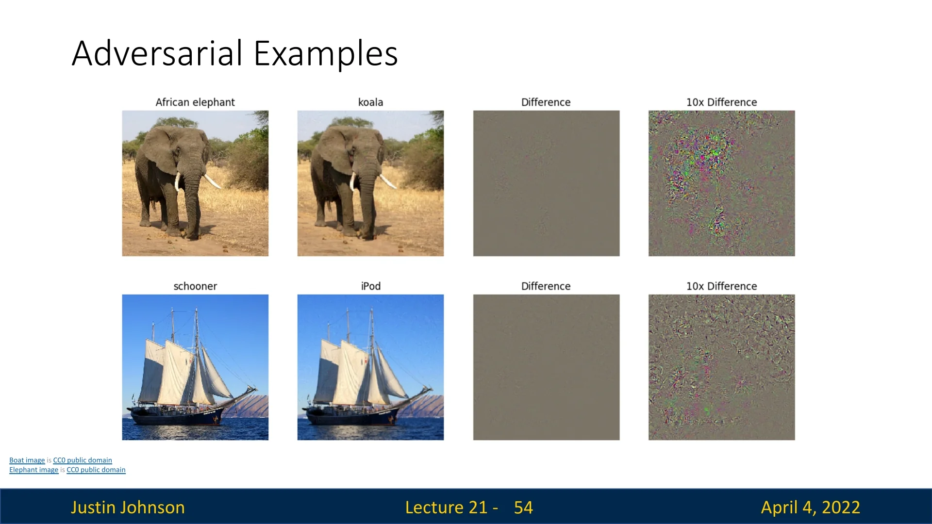
For a targeted attack (aiming to force classification into a specific wrong class \( c' \)), this objective can be formalized as: \[ I^{\ast } = \arg \max _{I} \left ( \underbrace {S_{c'}(I)}_{\mbox{target class score}} - \lambda \cdot \underbrace {\|I - I_{\mbox{orig}}\|_\infty }_{\mbox{perturbation magnitude}} \right ), \] where \( S_{c'}(I) \) is the model’s output score for the target class \( c' \), and the regularization term \( \lambda \cdot \|I - I_{\mbox{orig}}\|_\infty \) ensures that the perturbation remains small enough to be imperceptible to humans.
In essence, adversarial attacks are a malicious repurposing of the same gradient-based tools we previously used for interpretability—now aimed not at understanding the model, but at exposing its most brittle failure modes.
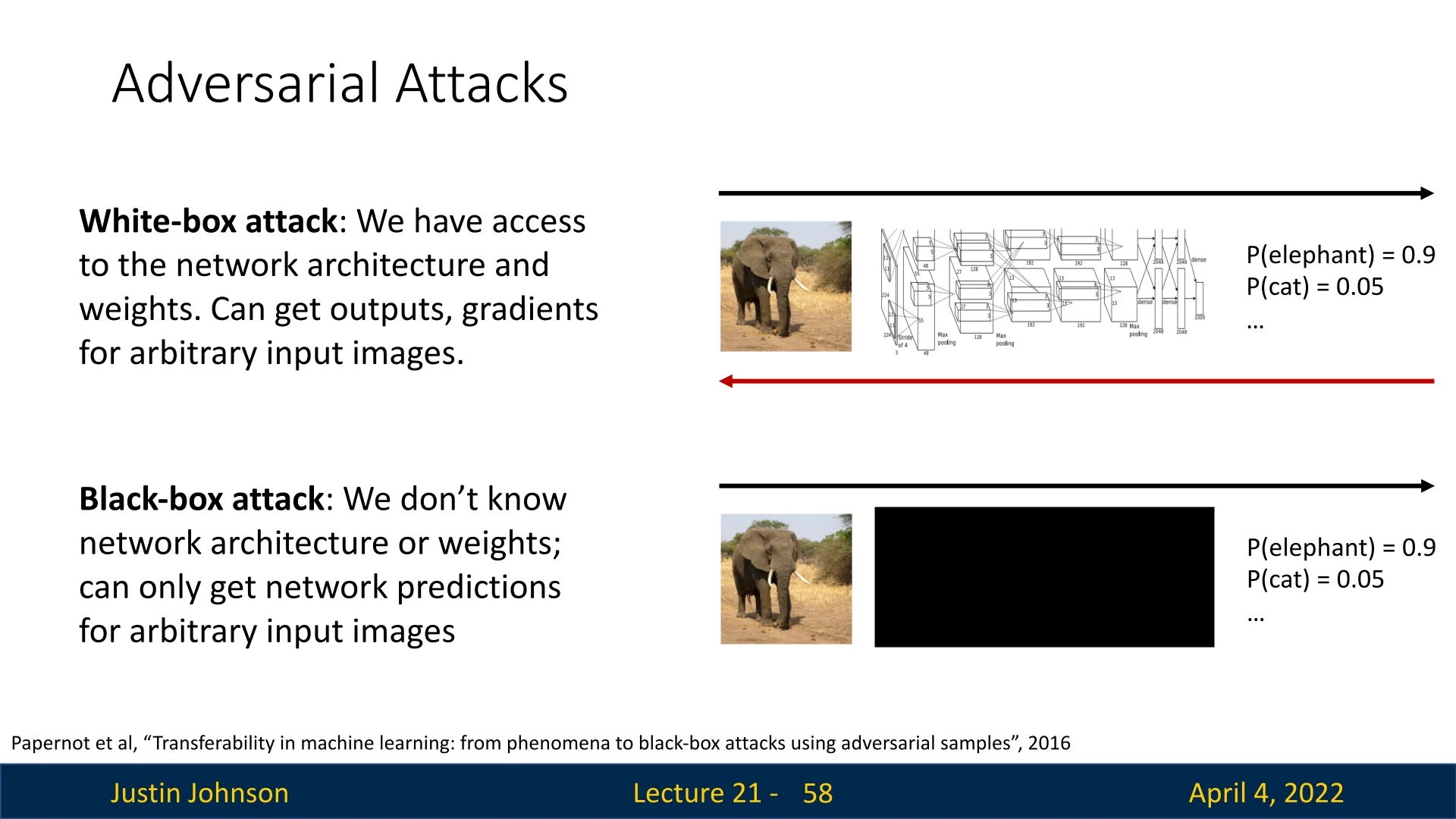
21.7.2 Taxonomy of Adversarial Attacks
White-box attacks These attacks assume full ”glass-box” visibility into the model (architecture, weights, gradients), enabling highly effective, gradient-based perturbations:
- FGSM (Fast Gradient Sign Method) [187]: One-step attack. Computes the gradient of the loss w.r.t. input once and perturbs each pixel by \(\epsilon \) in the direction that maximizes loss—fast but often coarse.
- BIM / I-FGSM (Basic / Iterative FGSM): Applies FGSM multiple times with smaller step size and clips after each step. This yields more refined perturbations under the same \(\|\cdot \|_\infty \le \epsilon \) constraint.
-
PGD (Projected Gradient Descent) [424]: Widely regarded as the strongest first-order adversary, PGD is a principled, iterative attack that maximizes model loss while strictly enforcing an imperceptibility constraint on the perturbation. It is a cornerstone of both adversarial evaluation and adversarial training [424].
- Random Initialization within the \(\epsilon \)-ball: Unlike FGSM or BIM, PGD begins not from the original input \( x_{\mbox{orig}} \), but from a randomly chosen point within the \(\ell _\infty \)-ball of radius \( \epsilon \). This random initialization allows the attack to explore more directions in the loss landscape, increasing the chance of escaping local optima and locating truly worst-case perturbations.
- Gradient Ascent + Projection Loop: PGD performs multiple steps of gradient ascent on the loss: \[ x^{(t+1)} = \Pi _{\mathcal {B}_\infty (x_{\mbox{orig}}, \epsilon )} \left ( x^{(t)} + \alpha \cdot \mbox{sign} \left ( \nabla _x \mathcal {L}(x^{(t)}, y) \right ) \right ) \] Each gradient step pushes the input in a direction that increases the loss. The projection operator \( \Pi \) then clips the result back into the \(\ell _\infty \)-ball: \[ \mathcal {B}_\infty (x_{\mbox{orig}}, \epsilon ) = \left \{ x : \|x - x_{\mbox{orig}}\|_\infty \leq \epsilon \right \} \] ensuring that no pixel is perturbed by more than \( \epsilon \). This enforces imperceptibility and validity at every step.
Why projection is crucial: Even small gradient steps can overshoot valid bounds—either violating the \( \ell _\infty \) constraint or pushing pixel values outside the allowable range (e.g., [0, 1]). The projection step acts like a tether, reeling the point back into the valid neighborhood around \( x_{\mbox{orig}} \), thus preserving visual indistinguishability.
Intuition: Imagine trying to find the highest point (worst-case misclassification) within a tiny neighborhood around your current location (the original image), while being tethered by a rope of length \( \epsilon \). PGD lets you take purposeful, uphill steps in the loss landscape—but if you stray too far, the rope snaps you back into the permissible region. This ensures that the adversarial example remains both effective and imperceptible.
PGD is not only a powerful attack—it also defines a training-time adversary in robust optimization formulations. Its widespread adoption stems from its ability to systematically approximate the worst-case error within a constrained region, making it the de facto benchmark for evaluating model robustness.
-
Carlini–Wagner (C&W) [67]: A precision attack that solves an explicit optimization problem. Instead of using sign gradients, C&W jointly minimizes:
(i) a distortion loss (e.g., \(\|\delta \|_2\)) to keep the perturbation minimal, and (ii) a classification loss that forces the model to misclassify with high confidence.
This targeted, optimization-based approach produces extremely small perturbations that often break even robust models with imperceptible changes. Unlike FGSM, which takes a single sign-based step, C&W adapts both direction and magnitude of every pixel.
Black-box attacks In these, the attacker has no access to gradients or model internals:
-
HopSkipJump [82]: A decision-based algorithm using only final class labels:
- 1.
- Initialization: Requires a starting adversarial example (any misclassified image).
- 2.
- Boundary search: Performs binary search along the line from the initial example to the original image to find the closest point on the decision boundary.
- 3.
- Gradient estimation: Samples around that boundary point, using model outputs to estimate a direction that moves toward the original image while staying adversarial.
- 4.
- Projection steps: Iteratively take steps along the estimated direction, projecting back onto the boundary, refining the adversarial example.
This boundary-walking strategy efficiently finds small perturbations with few queries.
- Transfer attacks: Utilize the fact that adversarial examples often transfer across different models. By crafting perturbations on a surrogate model (e.g., using FGSM, BIM, PGD), the attacker can often fool the target model without any queries.
-
Universal perturbations [454]: A single perturbation \(\delta \) that fools the model across many inputs:
- 1.
- Initialize \(\delta = 0\).
- 2.
- For each dataset image \(x\):
- If \(x + \delta \) is not adversarial, compute a minimal per-image perturbation \(\delta _x\).
- Update \(\delta \leftarrow \delta + \delta _x\) and project within an \(\epsilon \)-ball.
- 3.
- Repeat until \(\delta \) consistently causes misclassification across the dataset.
This demonstrates a global vulnerability—some directions in input space universally degrade model performance.
21.7.3 Milestones in Robustness Evaluation
- Carlini–Wagner attack [67]: Marked a turning point in adversarial research by defeating many proposed defenses like defensive distillation. It prompted a deep reassessment of what constitutes genuine robustness.
- Obfuscated gradients [648]: Revealed that many “robust” models only masked gradients, rather than solving the underlying problem. This discovery exposed a major flaw in evaluation protocols for robustness.
- Ensemble critique [66]: Demonstrated that naive ensembles of weak defenses do not produce strong robustness, highlighting the need for principled combinations or fundamentally stronger strategies.
- Cross-modality attacks [68]: Showed that adversarial vulnerabilities transcend modality boundaries, enabling attacks to transfer across vision and language models in multimodal architectures.
21.7.4 Defense Toolbox and Its Limitations
- Adversarial training [424]: The most empirically effective defense, achieved by injecting adversarial examples into the training loop. While it improves robustness, it significantly increases computational cost and may reduce clean accuracy. Its effectiveness is often constrained to the specific attack types seen during training.
- Input preprocessing: Simple techniques like JPEG compression, denoising, or spatial smoothing aim to “clean” adversarial noise. Though computationally cheap, they are largely ineffective against adaptive attacks designed to survive such transformations.
- Certified defenses: Provide provable guarantees that no perturbation within a given \(\ell _p\) radius can alter the model’s prediction. Techniques such as interval bound propagation and randomized smoothing are promising but face challenges in scalability and tightness of bounds.
- Architectural approaches: Aim to build inherently robust networks via design, e.g., enforcing Lipschitz continuity, smoothing activations, or using specialized robust layers. While theoretically appealing, these methods remain less mature and are still an active area of research.
21.7.5 Real-World Relevance and Persistent Risks
Adversarial examples are not just a lab curiosity—they remain adversarial even after transformations like printing, rephotographing, or 3D rendering. Notable risk areas include:
- Autonomous driving: Adversarial stop signs or lane markings can mislead onboard vision systems.
- Facial recognition: Perturbed accessories (e.g., adversarial eyeglasses) can cause identity spoofing.
- Medical imaging: Subtle modifications to radiology scans can alter diagnostic outcomes.
21.7.6 Open Challenges and Theoretical Connections
Crafting effective attacks remains easier than building robust models. Recent work connects adversarial vulnerability to phenomena like deep double descent [459], where highly overparameterized models exhibit brittle decision boundaries. Understanding and bridging this generalization–robustness gap is a central open problem in modern deep learning.
21.8 Class Activation Mapping (CAM) and Grad-CAM
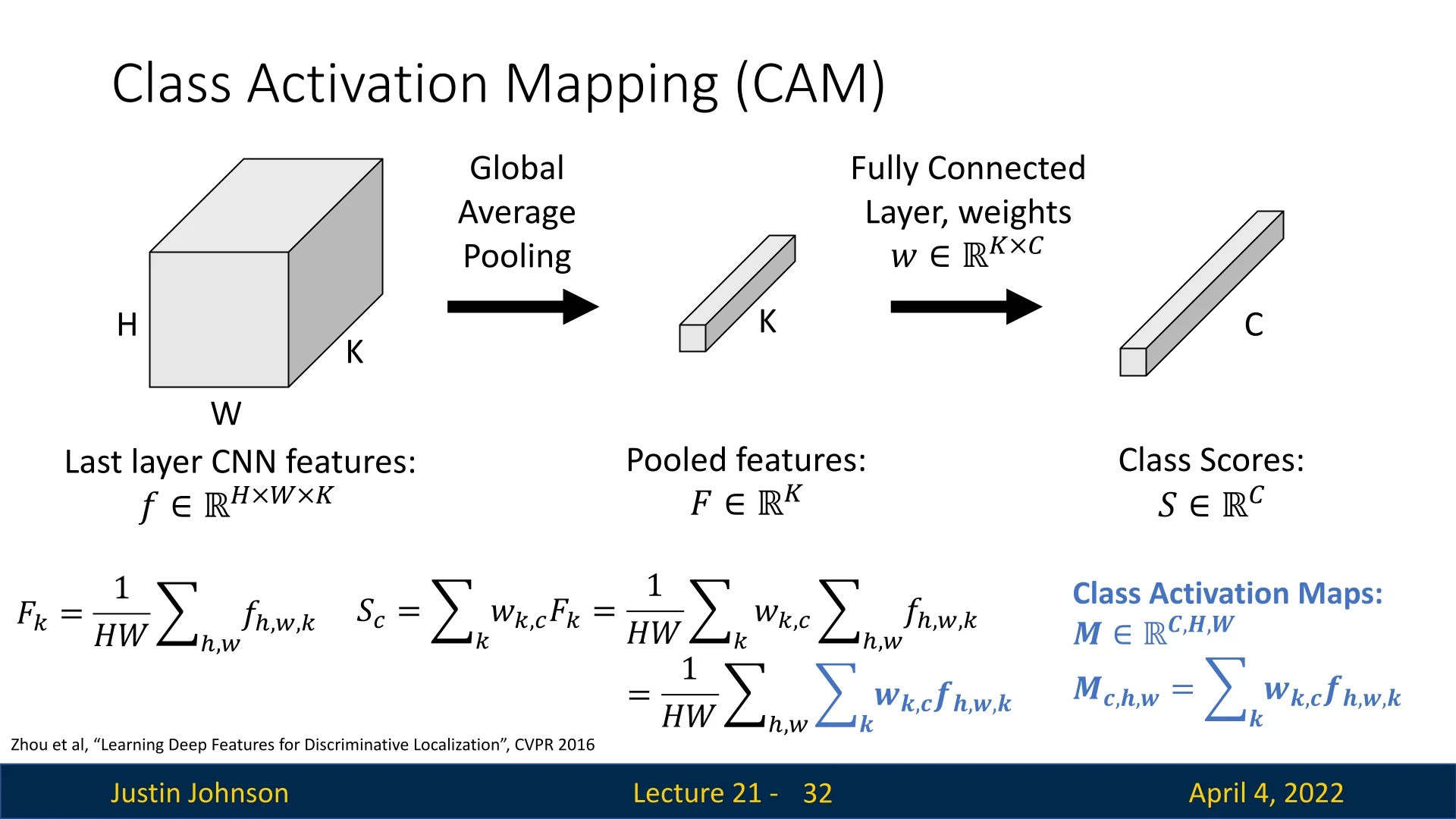
Class Activation Mapping (CAM) [816] is a visualization technique that highlights regions in an image which are important for a CNN’s classification decision. It operates by projecting the weights from the final fully connected (FC) layer back onto the feature maps of the last convolutional layer.
Mechanism of CAM Class Activation Mapping (CAM) [816] provides a way to localize the spatial regions in an image that are most influential for a CNN’s classification decision. CAM relies on a specific architectural constraint: the final convolutional layer must be followed by a global average pooling (GAP) layer and a single fully connected (FC) layer that maps directly to class scores.
Let \( f_k(x, y) \) denote the activation at spatial location \( (x, y) \) of channel \( k \) in the final convolutional layer. After global average pooling, each feature map is reduced to a scalar: \[ F_k = \frac {1}{H \cdot W} \sum _{x=1}^{H} \sum _{y=1}^{W} f_k(x, y), \] where \( H \) and \( W \) denote the height and width of the feature map. These pooled features \( \{F_k\} \) are then fed into a linear classifier: \[ S_c = \sum _k w_k^{(c)} F_k, \] where \( w_k^{(c)} \) is the learned weight connecting feature map \( k \) to class \( c \) in the final FC layer.
Substituting the definition of \( F_k \) yields: \[ S_c = \sum _k w_k^{(c)} \left ( \frac {1}{H \cdot W} \sum _{x=1}^{H} \sum _{y=1}^{W} f_k(x, y) \right ) = \frac {1}{H \cdot W} \sum _{x=1}^{H} \sum _{y=1}^{W} \sum _k w_k^{(c)} f_k(x, y). \] This formulation reveals that the class score \( S_c \) is a global sum of spatial contributions from each location \( (x, y) \). The class activation map \( M_c(x, y) \) is then defined as the pre-pooled spatial contribution for class \( c \): \[ M_c(x, y) = \sum _k w_k^{(c)} f_k(x, y). \]
This results in a low-resolution heatmap \( M_c \) that highlights the importance of each spatial location for predicting class \( c \). Since the feature maps \( f_k(x, y) \) preserve spatial structure (albeit at reduced resolution due to downsampling), the map \( M_c \) can be upsampled (e.g., via bilinear interpolation) to align with the original image, allowing visual localization of discriminative regions.
Intuition. Each convolutional channel \( k \) responds to certain visual patterns (e.g., texture, shape). The weight \( w_k^{(c)} \) indicates how important that pattern is for class \( c \). CAM computes a weighted combination of these patterns over space, producing a heatmap that reveals where the class-specific evidence appears in the image.
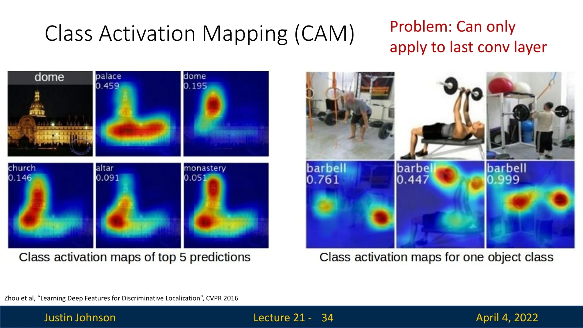
Limitations of CAM CAM is constrained by architecture: it only works with CNNs that end with a global average pooling layer directly connected to a linear classification head. This rules out many modern networks without such structure, including those with multiple FC layers or attention blocks. Moreover, CAM can only visualize the final convolutional layer, which may yield coarse localization due to its low spatial resolution. It lacks the flexibility to probe earlier layers or networks with more complex topologies. These limitations motivated the development of gradient-based generalizations such as Grad-CAM, which we now proceed to cover.
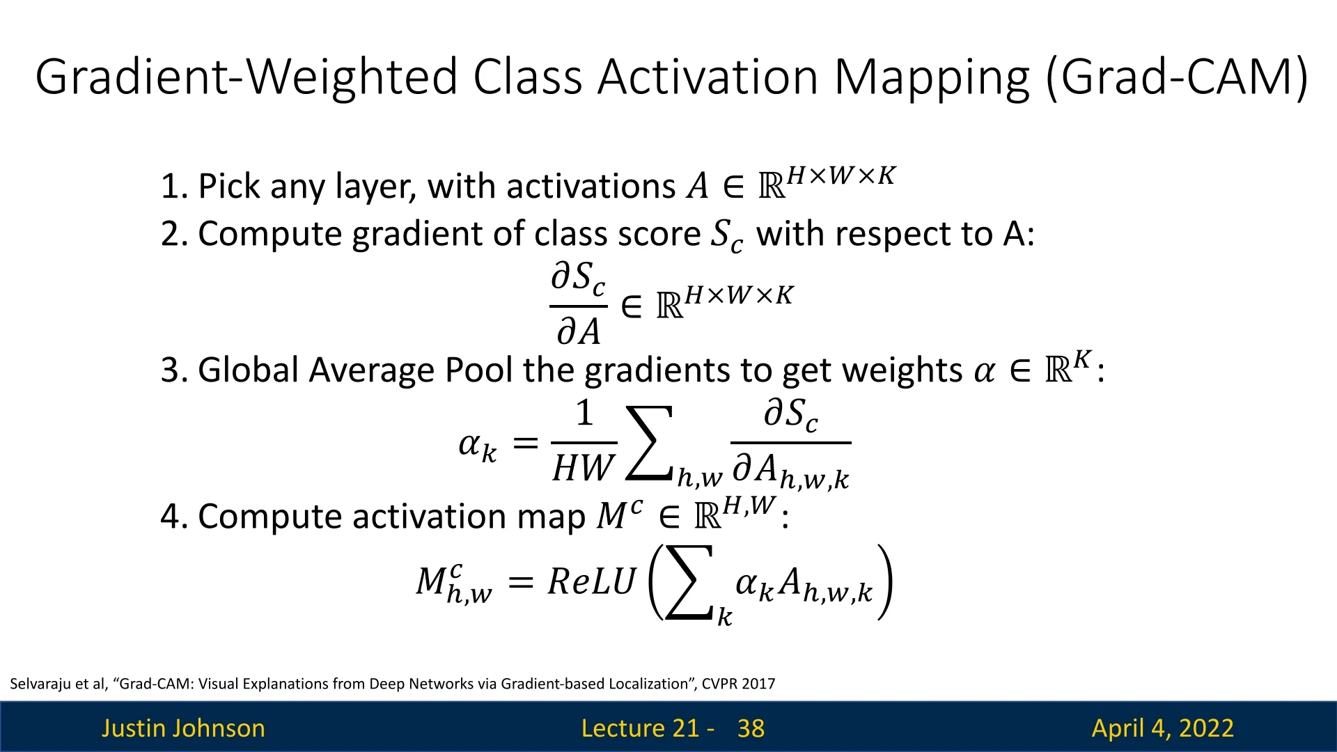
21.8.1 Generalization via Grad-CAM
Grad-CAM (Gradient-weighted Class Activation Mapping) [577] addresses these issues by using the gradients of any target class flowing into any convolutional layer to produce a localization map. The weights \( \alpha _k^c \) for each channel \( k \) are computed as: \[ \alpha _k^c = \frac {1}{Z} \sum _{i} \sum _{j} \frac {\partial S_c}{\partial A_{i,j}^k} \] where \( A^k \) is the activation map for channel \( k \), and \( S_c \) is the score for class \( c \). The final Grad-CAM map is: \[ M_c^{\mbox{Grad}} = \mbox{ReLU} \left ( \sum _k \alpha _k^c A^k \right ) \]
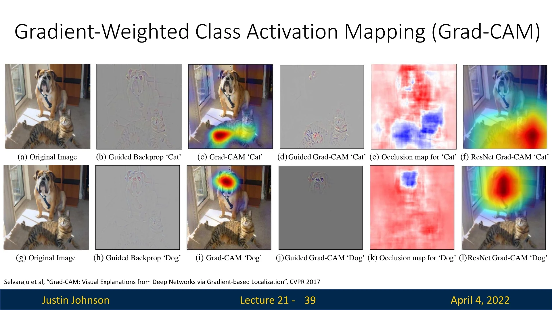
Comparative Visualization Examples Grad-CAM can be applied at any convolutional layer and in a wider range of networks. The following figure shows comparisons between guided backpropagation, Grad-CAM, and their combination for different classes (e.g., cat vs dog).
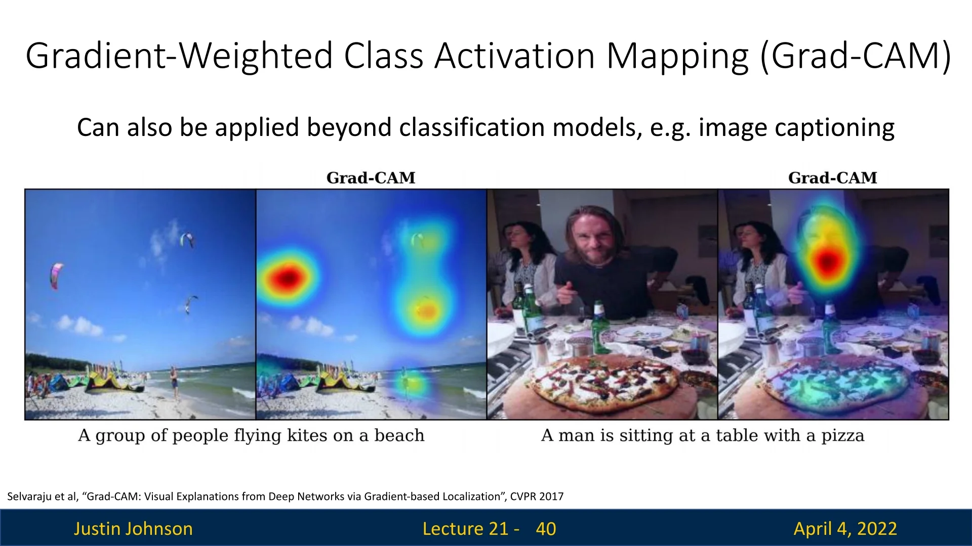
Grad-CAM is model-agnostic with respect to the output modality—it is not restricted to image classification. By leveraging the gradients flowing into any convolutional feature map, Grad-CAM can be extended to tasks like image captioning and visual question answering.
21.8.2 Comparison Between CAM and Grad-CAM
| Aspect | CAM | Grad-CAM |
|---|---|---|
| Architectural Requirement | Requires GAP before the FC classifier; limited to custom architectures. | No architectural constraints; works with standard CNNs like VGG or ResNet. |
| Weight Calculation | Uses fixed weights \( w_{k}^{(c)} \) from the final FC layer. | Computes dynamic weights \( \alpha _k^{(c)} \) via gradients of the class score. |
| Layer Applicability | Only the last conv layer before GAP. | Any convolutional layer, including early or intermediate ones. |
| Network Compatibility | Only with networks designed with GAP. | Works with any pretrained CNN without modification. |
| ReLU on Heatmap | Not explicitly applied; may include negative activations. | Applies ReLU to focus on positive class evidence. |
| Computational Cost | Low; forward pass only. | Higher; requires a backward pass to compute gradients. |
In summary, CAM introduced the concept of generating spatially localized class-specific heatmaps using fixed feature-to-class weights, but its reliance on specific architectures limited its general applicability. Grad-CAM resolved this by introducing dynamic, gradient-based weighting, allowing it to be broadly applied to modern CNNs with richer, multi-layer interpretability.
From Explanation to Synthesis: A Path Toward Feature Inversion CAM and Grad-CAM are valuable tools for interpreting neural networks by highlighting where the model looks when making a prediction. But they remain reactive—they analyze a network’s behavior given an input. What if we reversed this perspective?
Instead of asking “Where does the model look?”, we can ask “What does the model see?”. That is: can we reconstruct or synthesize an input image that would strongly activate a specific neuron, feature channel, or class output? This brings us to the domain of feature inversion—a class of methods that aim to decode and visualize the internal representations of neural networks by optimizing an input image to match hidden activations.
This generative view enables us to move beyond saliency and uncover the implicit visual concepts a model has learned, making it an essential next step in deep network interpretability.
21.9 Feature Inversion
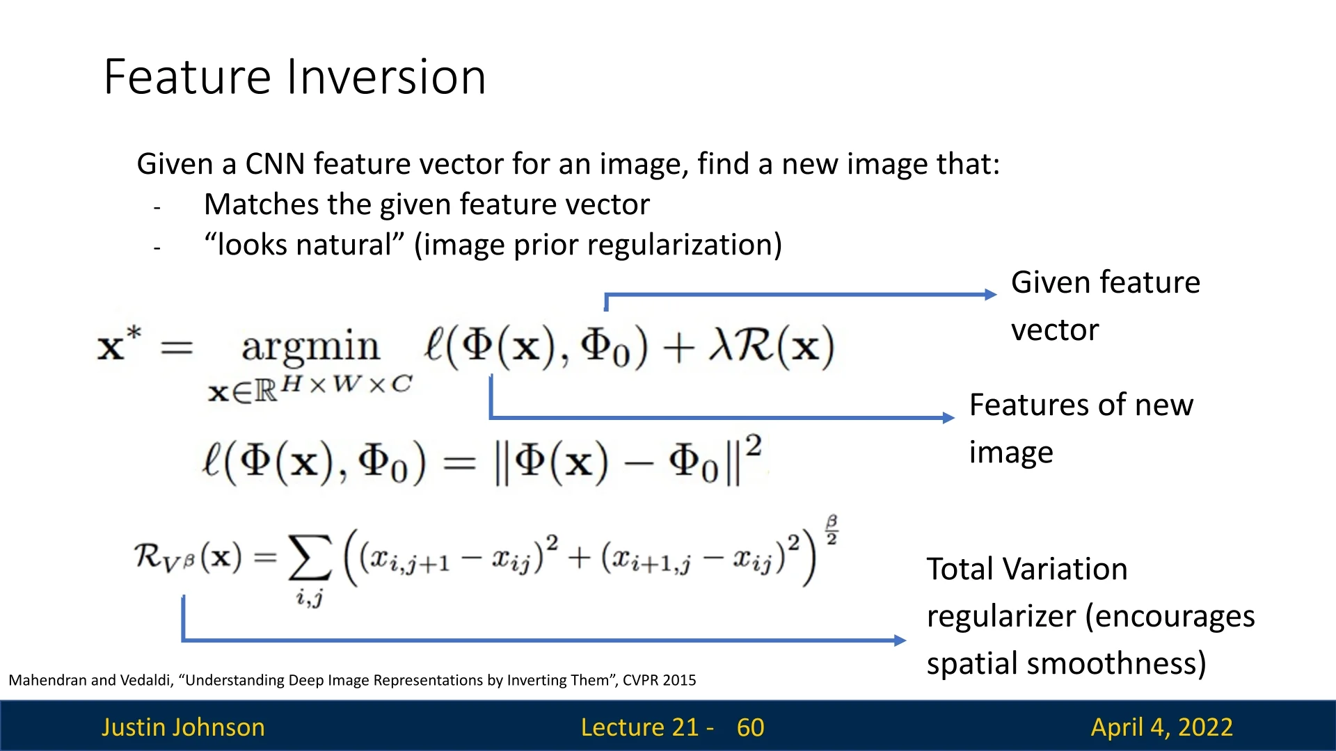
Feature inversion refers to the task of reconstructing an input image \( \mathbf {x}^* \) that corresponds to a given internal feature representation \( \Phi _0 \) extracted from a trained convolutional neural network (CNN). In contrast to gradient ascent—where we synthesize an image that maximally activates a particular neuron—feature inversion aims to recover an image whose intermediate features match those of a reference image.
Problem Formulation Let \( \Phi (\mathbf {x}) \in \mathbb {R}^d \) denote the feature vector extracted from an intermediate layer of a pretrained CNN when processing an image \( \mathbf {x} \in \mathbb {R}^{H \times W \times C} \). Given a target image \( \mathbf {x}_0 \), we define \( \Phi _0 = \Phi (\mathbf {x}_0) \). The goal is to reconstruct an image \( \mathbf {x}^* \) such that its feature embedding closely matches \( \Phi _0 \), while also ensuring that the reconstruction remains natural-looking.
\[ \mathbf {x}^* = \arg \min _{\mathbf {x} \in \mathbb {R}^{H \times W \times C}} \ell (\Phi (\mathbf {x}), \Phi _0) + \lambda \mathcal {R}(\mathbf {x}) \] \[ \ell (\Phi (\mathbf {x}), \Phi _0) = \|\Phi (\mathbf {x}) - \Phi _0\|^2 \]
Here, \( \mathcal {R}(\mathbf {x}) \) is a regularization term (e.g., total variation) that encourages spatial smoothness or other natural image priors:
\[ \mathcal {R}_{V^\beta }(\mathbf {x}) = \sum _{i,j} \left ( (x_{i,j+1} - x_{i,j})^2 + (x_{i+1,j} - x_{i,j})^2 \right )^{\frac {\beta }{2}} \]
Comparison to Gradient Ascent Feature inversion minimizes the difference between two fixed feature vectors. In contrast, gradient ascent attempts to maximize the activation of a particular neuron or class score:
\[ \mathbf {x}^* = \arg \max _{\mathbf {x}} f(\mathbf {x}) - \lambda \mathcal {R}(\mathbf {x}) \]
Thus, while gradient ascent highlights what inputs cause strong responses, feature inversion reconstructs what input could have plausibly produced a given representation.
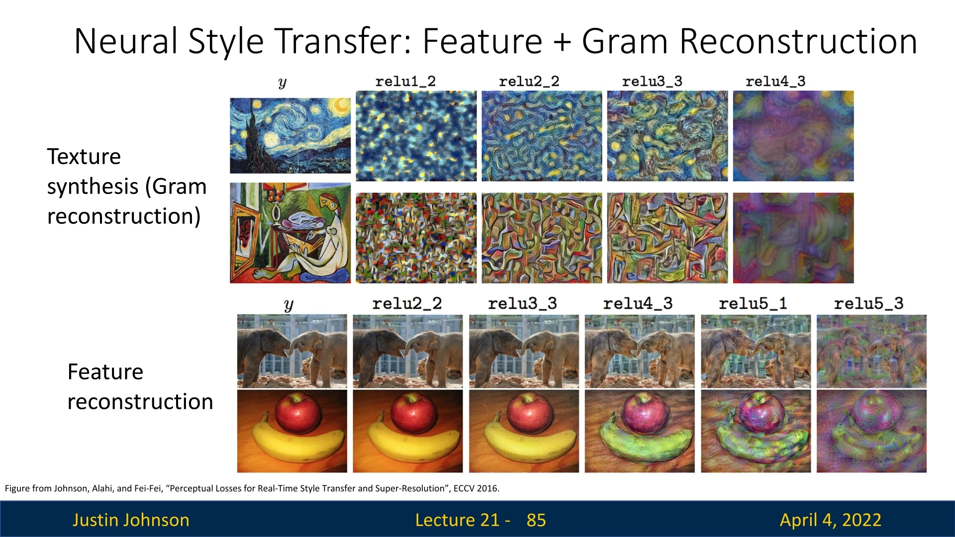
Effect of Layer Depth The fidelity of reconstructed images depends on the depth of the feature layer:
- Shallow layers: Preserve local textures, colors, and edges. Reconstructions are often nearly photorealistic.
- Deeper layers: Emphasize high-level semantics and invariance, discarding fine details. Reconstructions become abstract or blurry.
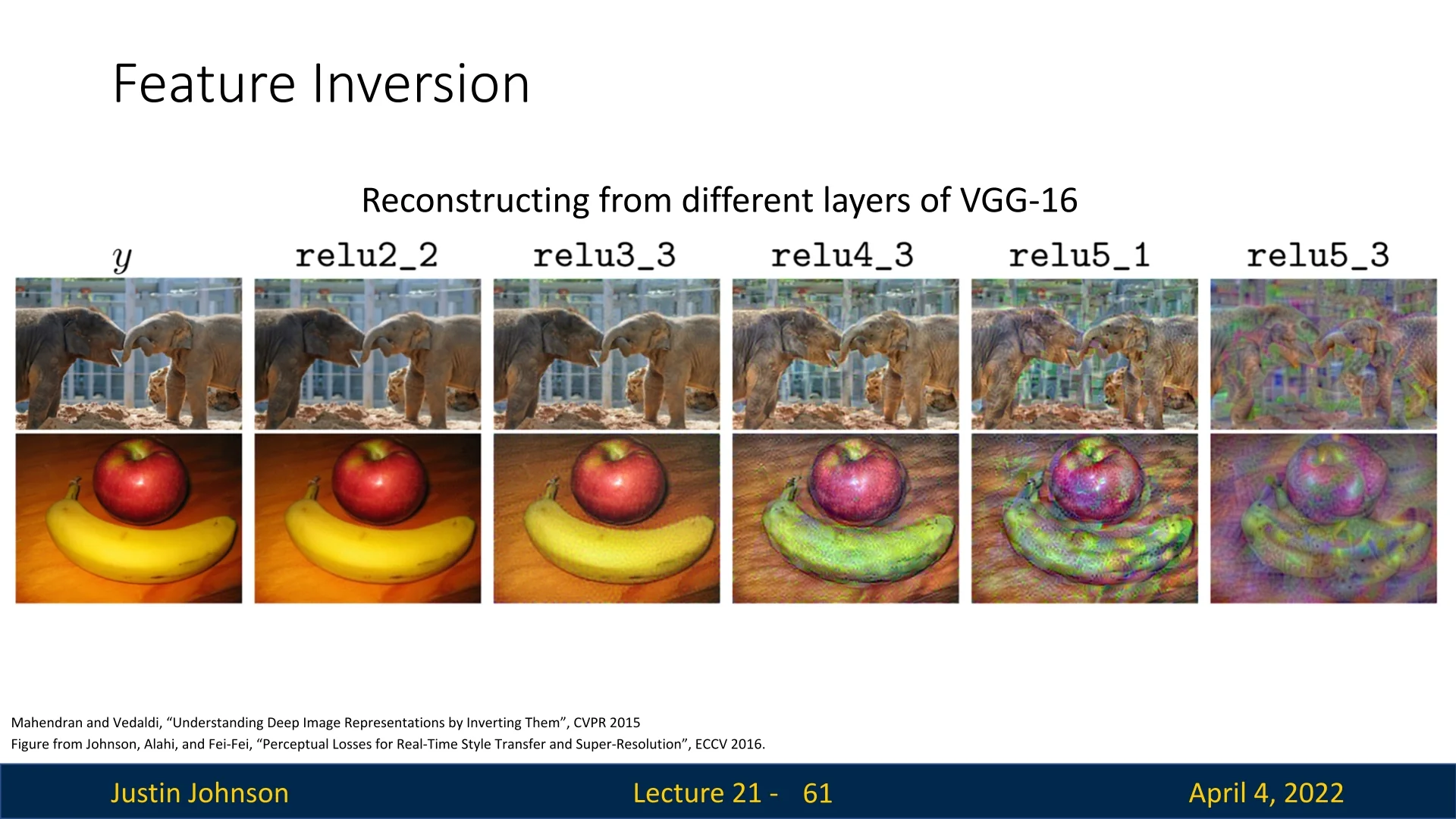
Interpretability Insights Feature inversion provides an intuitive, visual understanding of what information is preserved at each stage of processing inside a CNN. It reveals how much of the original image is retained or lost—both in low-level visual content and high-level semantic abstraction.
Applications Beyond interpretability, feature inversion has been used in:
- Visualizing latent representations in self-supervised learning.
- Debugging representations in transfer learning pipelines.
- Data-free knowledge distillation and training set recovery.
Beyond Feature Inversion While feature inversion focuses on reconstructing images that faithfully match internal representations, one can also explore how these representations transform an image when amplified. By nudging the input in directions that increase certain layer activations, the network begins to impose its learned abstractions onto the image—accentuating patterns, textures, or objects it has internalized. This approach underlies the technique popularized by Google’s DeepDream, where gradient ascent is applied iteratively on a real image to enhance the presence of specific learned features. Depending on the layer selected, the result ranges from abstract texture hallucinations to fully formed semantic motifs, offering a surreal glimpse into the model’s internal visual vocabulary.
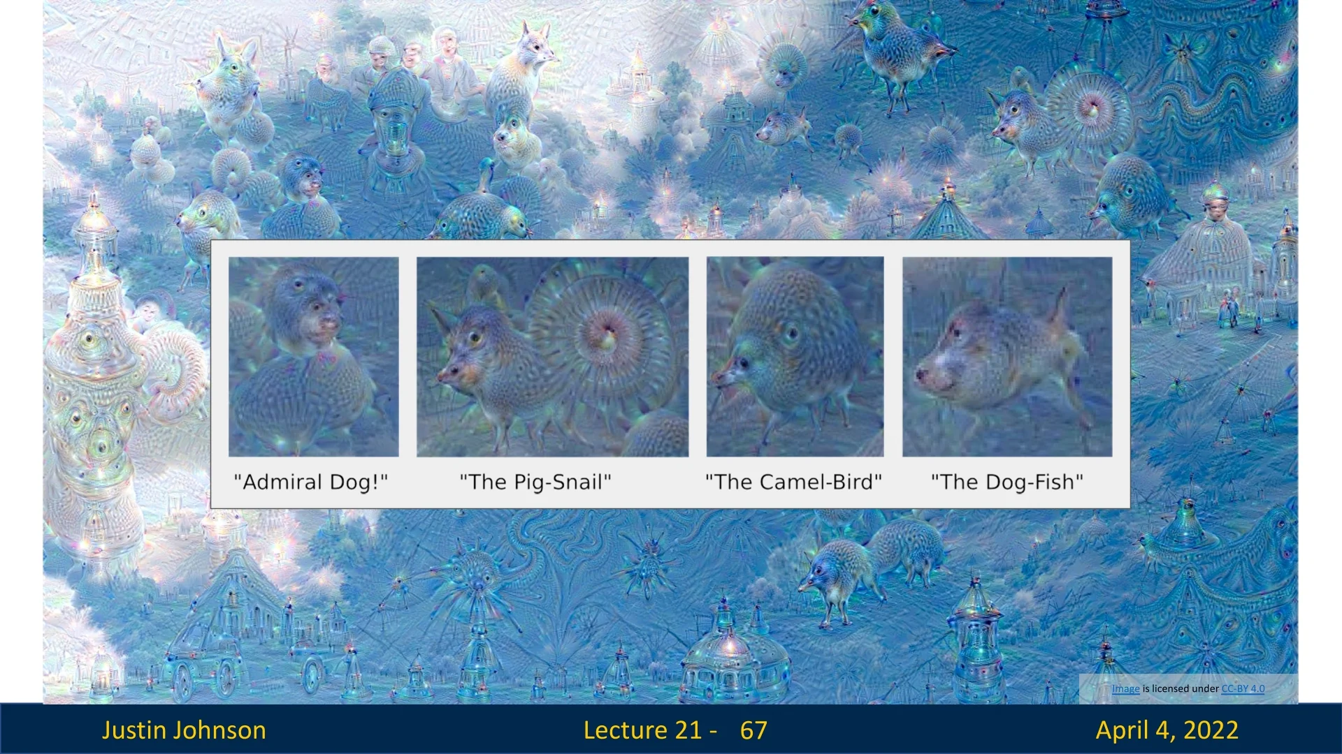
21.10 DeepDream: Amplifying Neural Perceptions
While feature inversion seeks to match internal representations of a specific image, DeepDream [455] instead aims to amplify patterns already present in a given image—revealing the ”visual concepts” that specific layers respond to. The result is often surreal and hallucinatory, reflecting the abstractions encoded within the network.
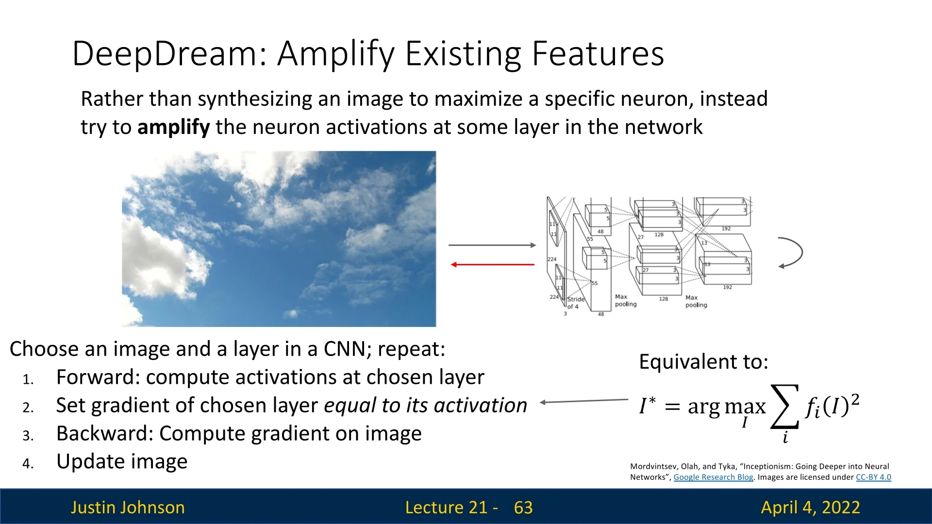
Optimization Objective Formally, given a fixed CNN and a chosen layer \( \phi \), DeepDream seeks to find an image \( I^{\ast } \) that maximizes the L2 norm of the feature activations at that layer: \[ I^{\ast } = \arg \max _I \|\phi (I)\|_2^2 + R(I) \] where \( R(I) \) denotes natural image regularization terms such as total variation, Gaussian blur, or pixel clipping. These are essential to ensure outputs remain visually coherent and human-interpretable.
Amplifying Layer-wise Semantics DeepDream acts like a feedback loop: it enhances the features already detected by a layer in the input image. The layer selected significantly influences the visual effect:
- Lower layers: Emphasize edges, colors, and textures. These effects tend to be localized and geometric.
- Higher layers: Reveal semantic abstractions—patterns resembling animals, eyes, buildings, or other high-level features.
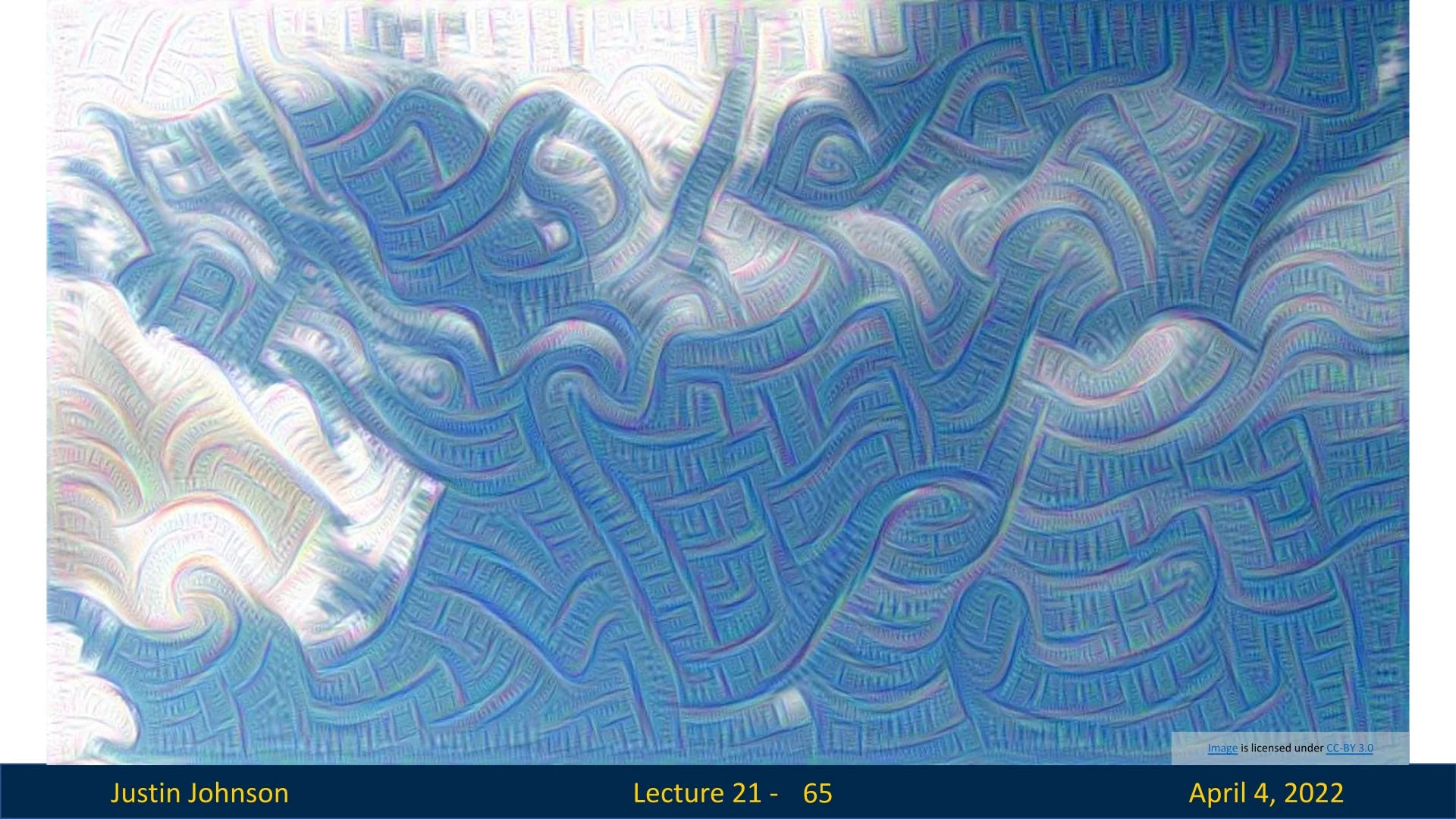
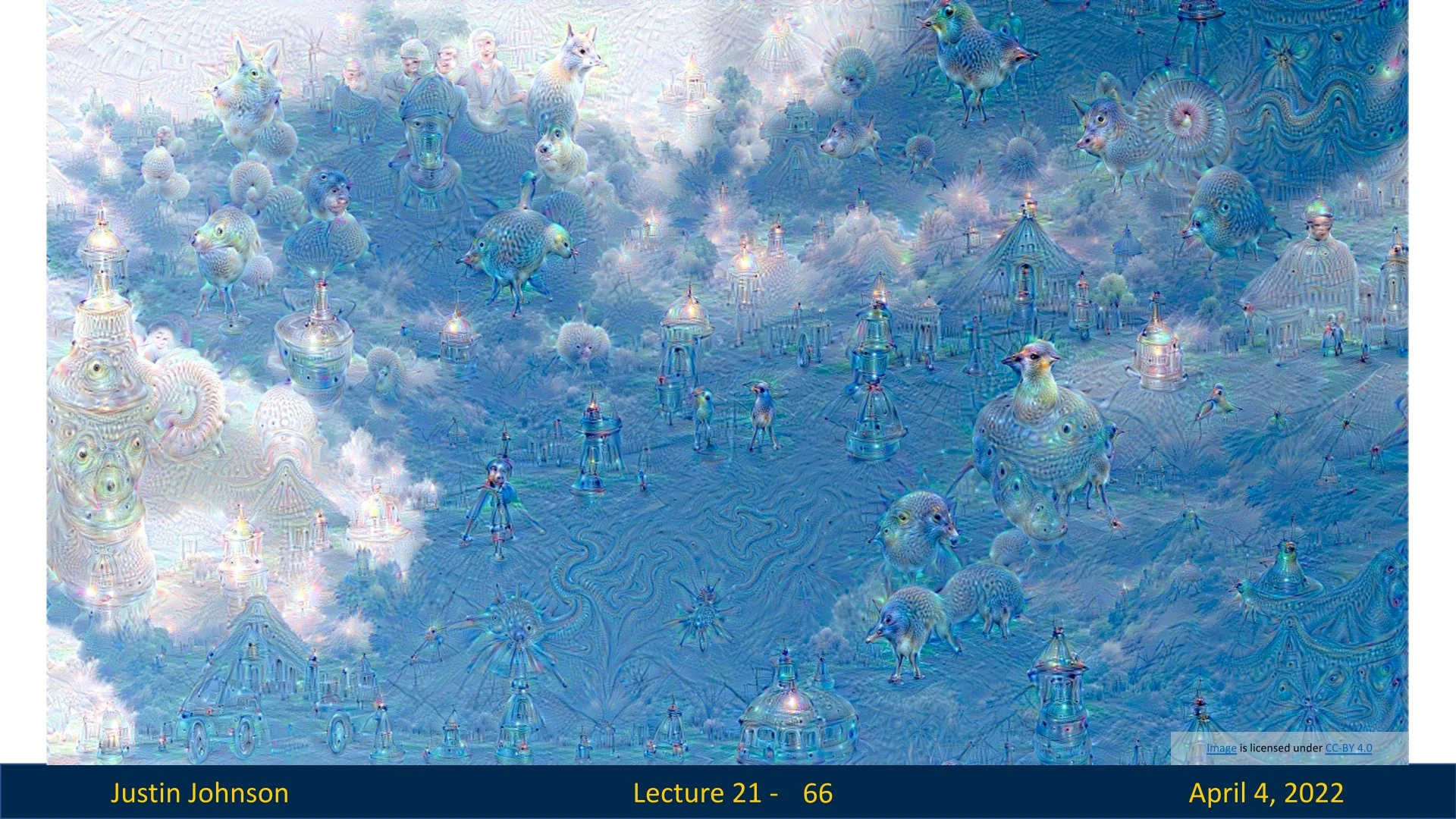
Dreaming Deeper The longer the optimization is run, the more pronounced the features become—and the farther the image drifts from its original content. In effect, the neural network is “dreaming” what it expects to see, iteratively shaping the image to match layer-wise priors.
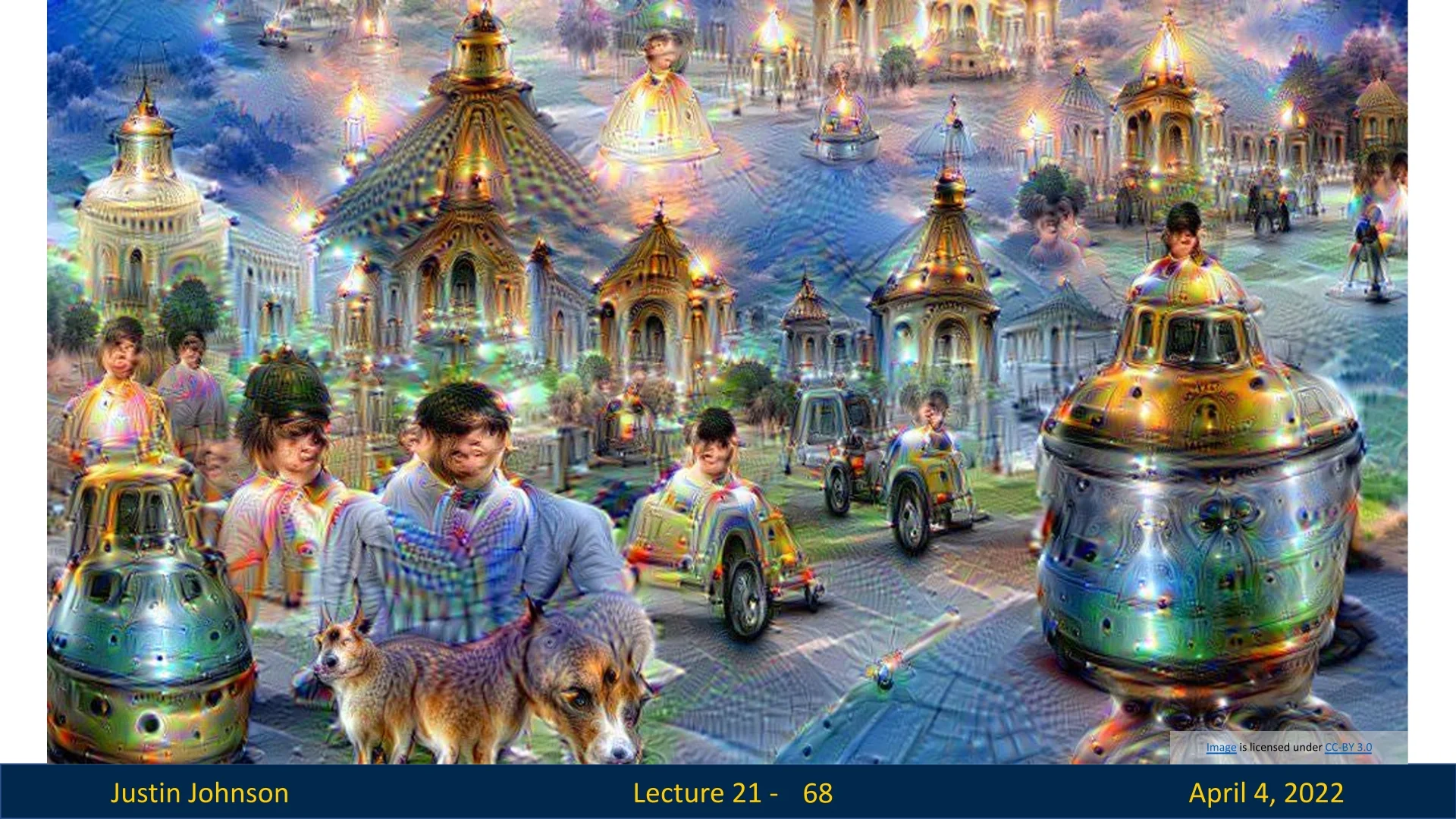
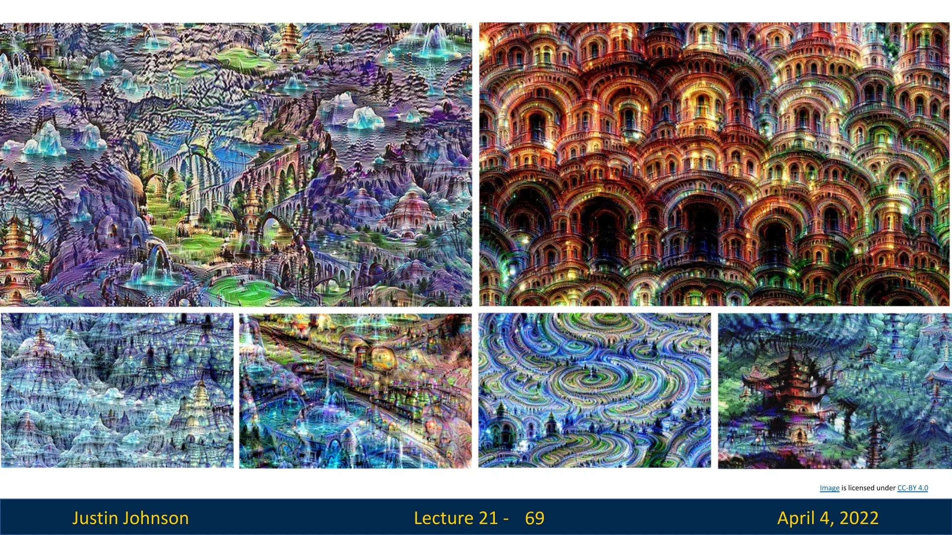
Interpretability Value Although DeepDream lacks the formal guarantees of analytical interpretability techniques, it offers a vivid and intuitive glimpse into what internal layers of a convolutional neural network are attuned to. By recursively amplifying activation patterns in natural images, it exposes the preferences of learned filters—ranging from edges and textures to object-like structures—across multiple layers of abstraction. In doing so, DeepDream serves as a creative tool that externalizes otherwise hidden visual concepts, blurring the line between model explanation and algorithmic art.
Perhaps more importantly, the emergence of repetitive motifs and rich, hallucinatory textures in DeepDream outputs reveals a key inductive bias of CNNs: their strong reliance on texture-like statistics, even in deeper semantic layers. This observation has inspired a wave of research into directly modeling such internal representations—not just for visualizing what a network has learned, but for synthesizing entirely new images governed by its internal feature distributions. Early approaches based on patch reassembly or nearest-neighbor texture transfer paved the way, but it was the work of Gatys, Ecker, and Bethge [173] that reframed texture as an optimizable property encoded in the second-order statistics (Gram matrices) of deep feature activations. This insight laid the foundation for the field of neural texture synthesis, which we explore next.
21.11 Texture Synthesis
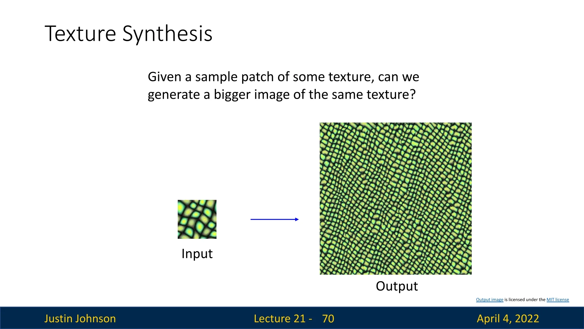
Texture synthesis aims to generate a larger image from a small input patch such that the output maintains similar local texture statistics. The goal is not to copy the input exactly, but to match its perceptual properties at the level of local patterns and structure.
Before diving into neural approaches to texture synthesis, it’s helpful to build intuition from the classical perspective. The task can be illustrated by providing a small texture sample—such as a patch of bricks or fabric—and asking the algorithm to generate a larger image that visually resembles it, without explicitly copying any region. This objective is illustrated in the below figure, followed by a classical nearest-neighbor approach that exemplifies one of the earliest and most influential strategies in this domain.
21.11.1 Classical Approaches
Early algorithms synthesize textures by directly copying pixels from a source image:
- Non-parametric sampling [141]: Grow the output image one pixel at a time in raster scan order, matching local neighborhoods using nearest-neighbor search.
- Tree-structured vector quantization [711]: Speeds up sampling using a hierarchical data structure for efficient neighborhood lookup.
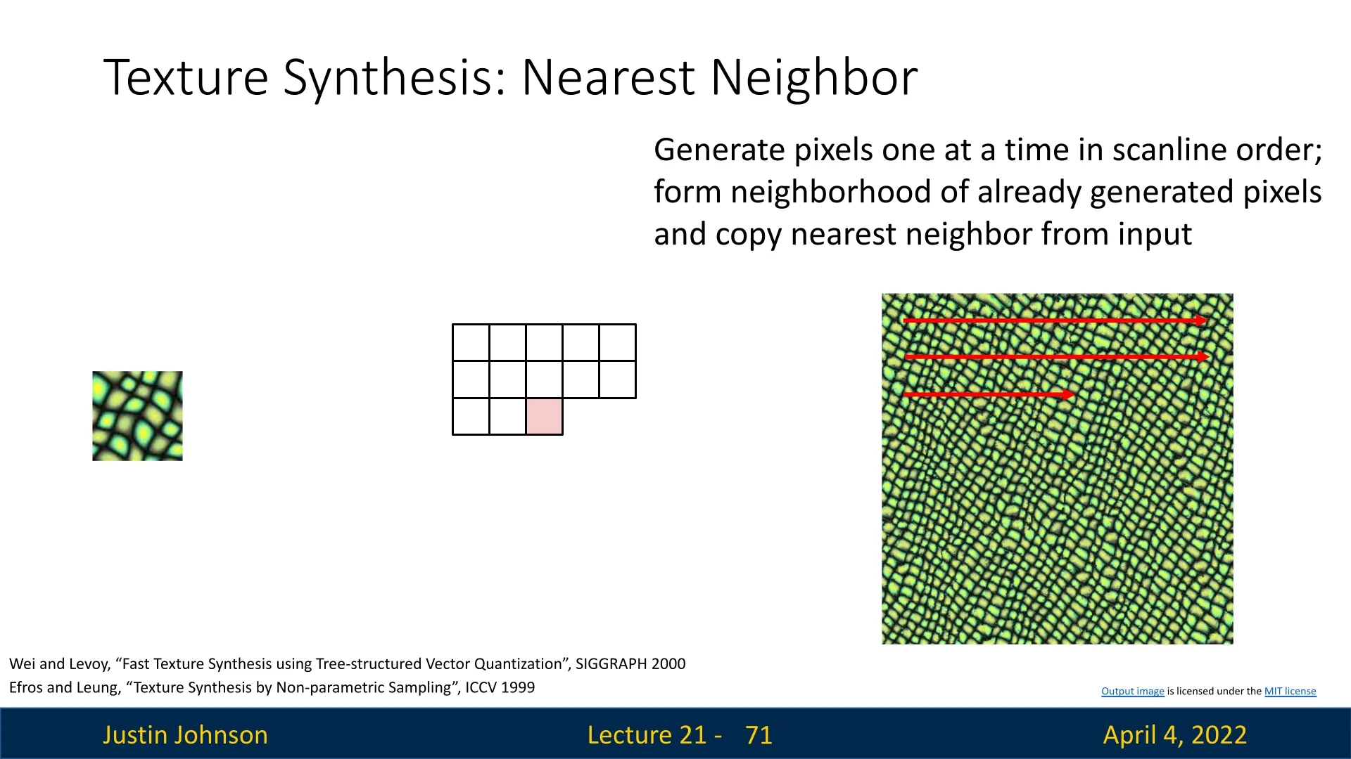
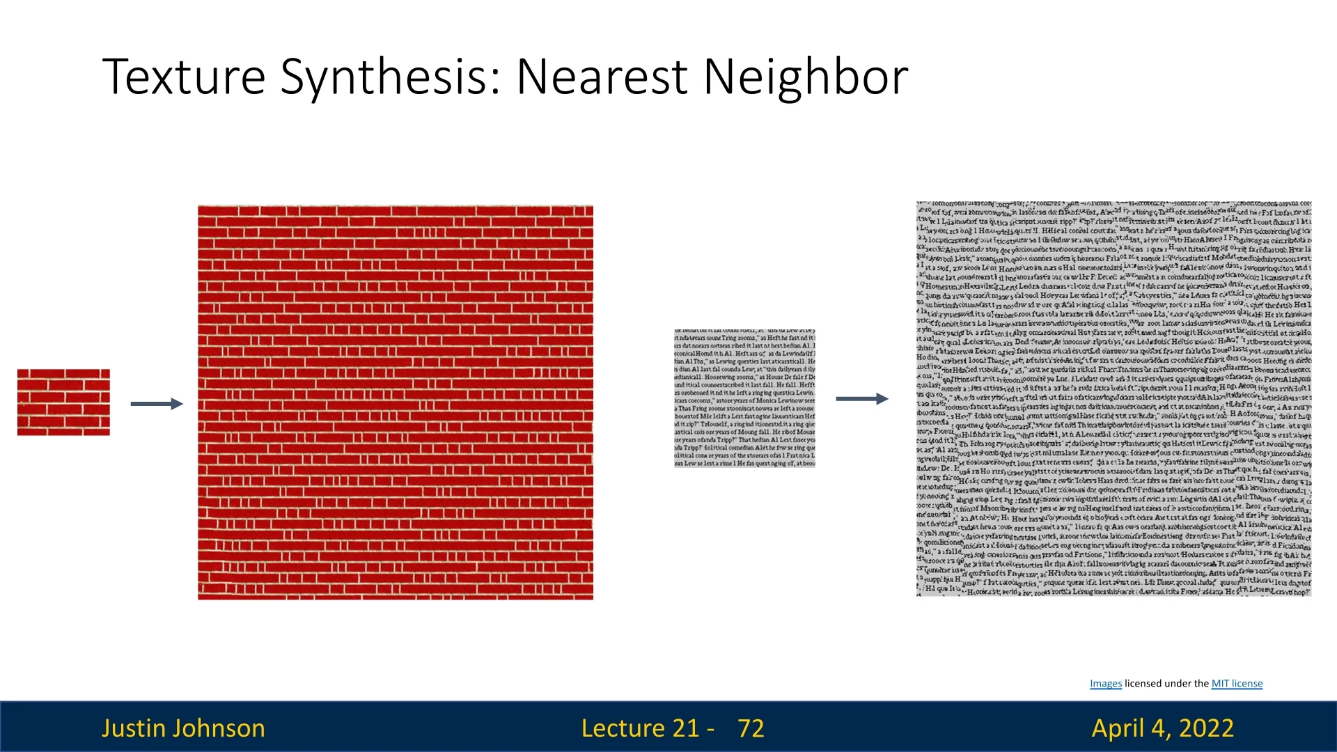
Limitations of Pixel Matching These techniques often fail on complex textures where pixel-level neighborhoods do not capture the underlying structure. They also lack flexibility for incorporating semantics or learning-based priors.
21.11.2 Neural Texture Synthesis via Gram Matrices
Gatys et al. [173] proposed a landmark approach to texture synthesis using convolutional neural networks pretrained on large-scale image datasets. Rather than matching image pixels directly, their method captures texture by aligning the second-order statistics of intermediate activations in a CNN. These statistics are encoded using Gram matrices, which measure feature co-activation patterns while discarding explicit spatial information.
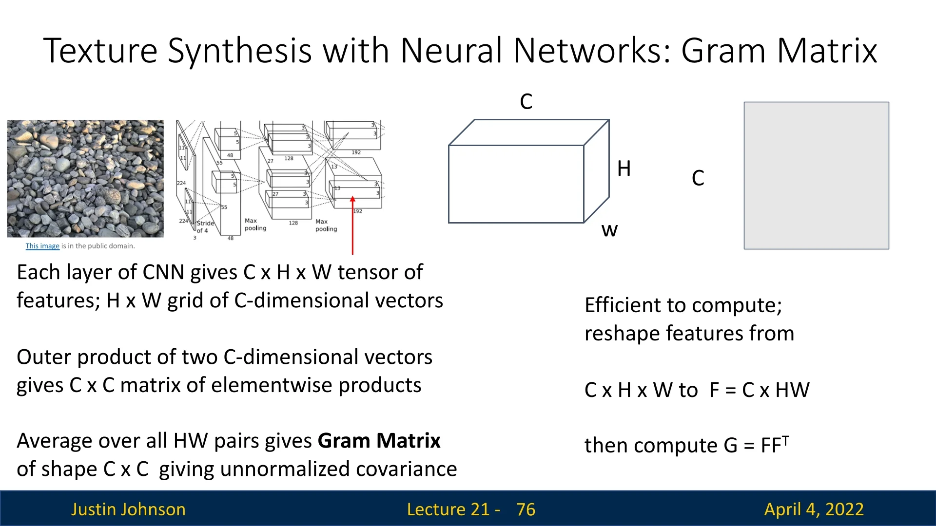
Constructing the Gram Matrix Given a feature map tensor \( F^{\ell } \in \mathbb {R}^{C_\ell \times H_\ell \times W_\ell } \) at some layer \( \ell \), we compute the corresponding Gram matrix \( G^{\ell } \in \mathbb {R}^{C_\ell \times C_\ell } \) as: \[ G^{\ell }_{c,c'} = \sum _{h,w} F^{\ell }_{c,h,w} \cdot F^{\ell }_{c',h,w} \] Each entry \( G^{\ell }_{c,c'} \) represents the inner product between feature maps \( c \) and \( c' \) across all spatial locations. This effectively measures the extent to which features \( c \) and \( c' \) co-occur in the image, averaged over space.
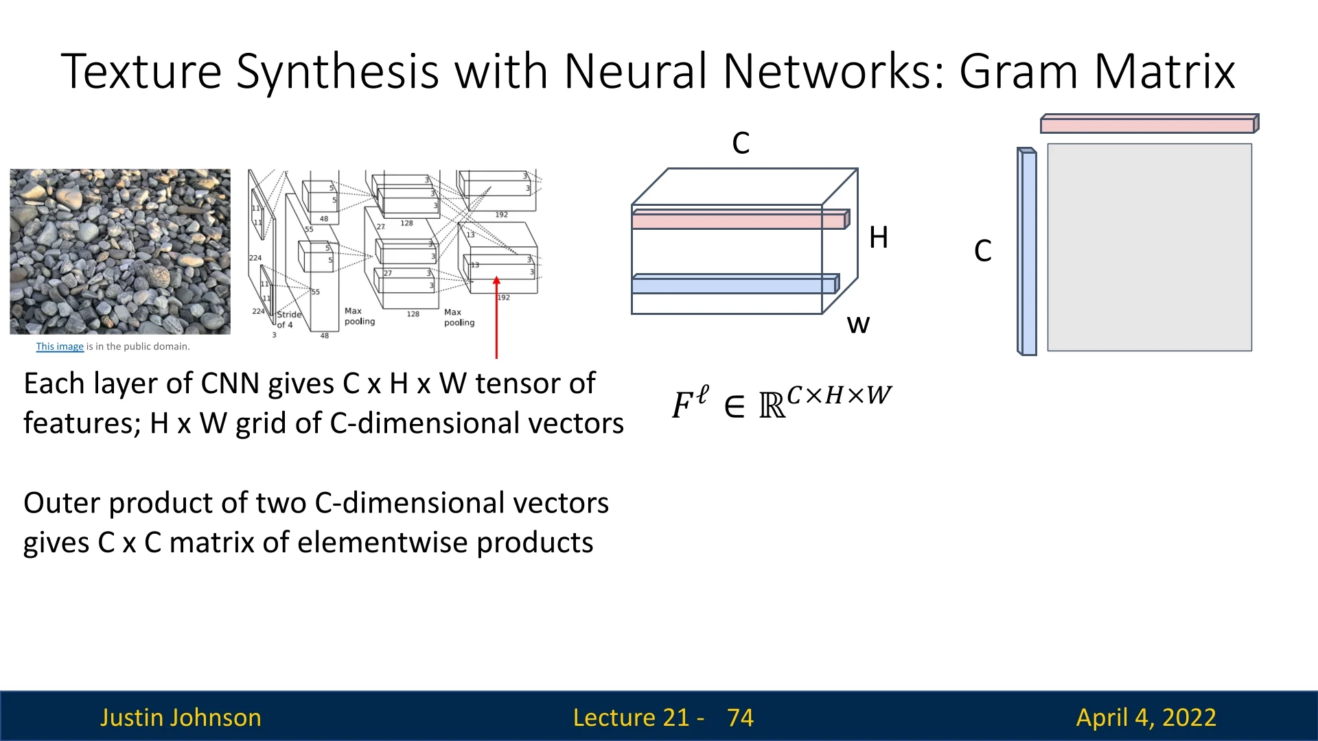
Why Gram Matrices? Textures are often characterized by the statistical relationships between local patterns rather than their precise spatial arrangement. By aggregating over spatial locations, the Gram matrix retains feature co-activation statistics while discarding spatial structure—making it ideally suited for texture modeling.
Computationally, this becomes efficient by reshaping \( F^{\ell } \) from shape \( C \times H \times W \) into a matrix \( F \in \mathbb {R}^{C \times (H W)} \), and computing: \[ G = F F^\top \in \mathbb {R}^{C \times C} \] This formulation allows fast matrix multiplication instead of nested loops, making it tractable even for deep layers with large spatial dimensions.
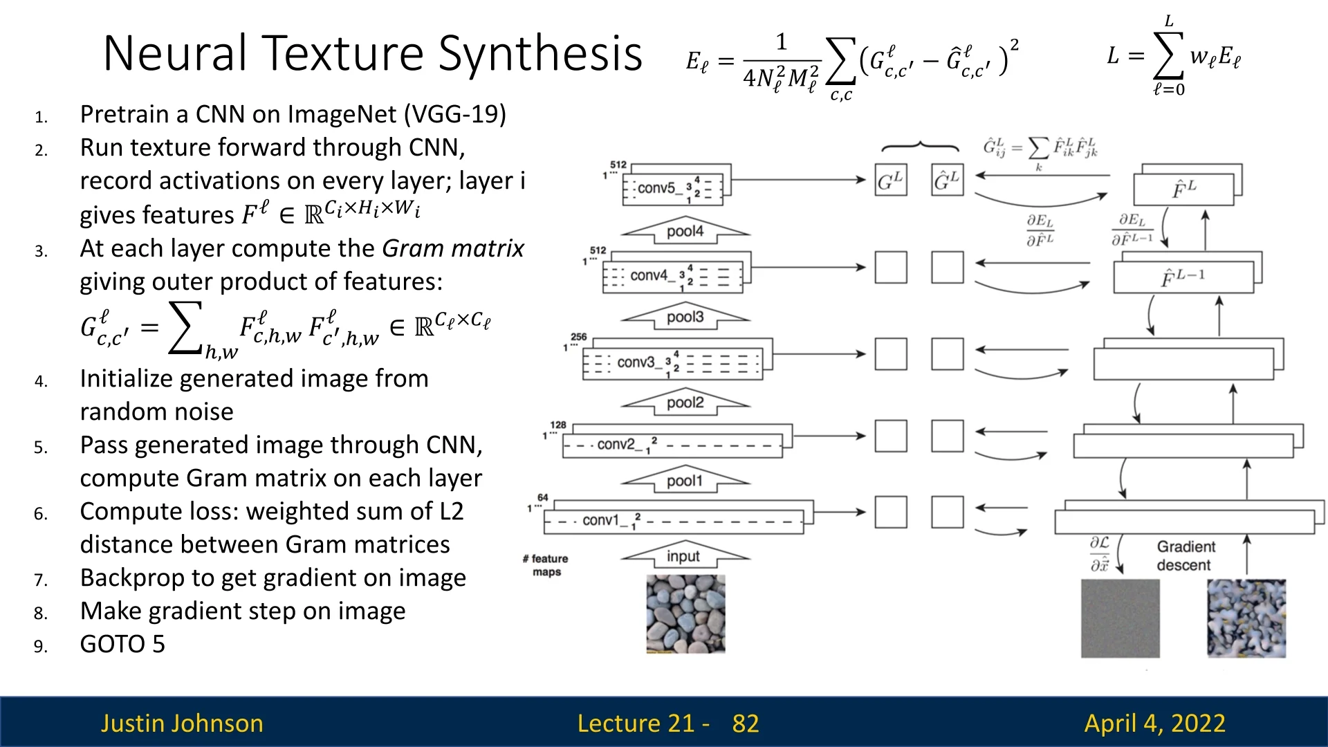
Optimization Pipeline The texture synthesis process is driven by matching the Gram matrices of a generated image to those of a reference texture image, across multiple CNN layers. The full algorithm is:
- 1.
- Use a pretrained CNN (e.g., VGG-19) and record feature activations \( F^{\ell } \) at selected layers for a given texture image.
- 2.
- Compute Gram matrices \( G^{\ell } \) from these activations.
- 3.
- Initialize the synthesized image \( I \) from white noise.
- 4.
- Iterate:
- Forward \( I \) through the CNN to compute new Gram matrices \( \hat {G}^{\ell } \).
- Compute per-layer style loss: \[ E_\ell = \frac {1}{4N_\ell ^2 M_\ell ^2} \sum _{c,c'} \left ( G^{\ell }_{c,c'} - \hat {G}^{\ell }_{c,c'} \right )^2 \]
- Aggregate across layers: \( L = \sum _{\ell } w_\ell E_\ell \)
- Backpropagate to update the image \( I \).
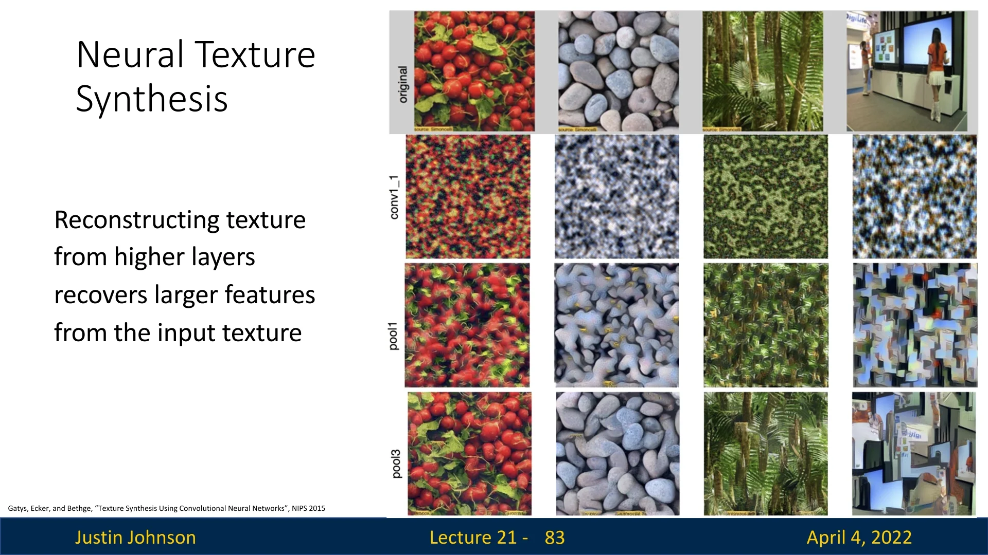
Effect of Matching Higher Layers Different layers encode different types of information: lower layers capture fine-scale patterns such as edges or color blobs, while deeper layers encode more abstract texture features. By matching Gram matrices at higher layers, the synthesized texture captures broader patterns and global structure—though precise spatial detail may be lost.
Impact and Legacy The Gram-based synthesis approach laid the foundation for two influential lines of work:
- Neural Style Transfer – Separates style (texture) and content by combining Gram matrix loss with feature reconstruction loss [172].
- Fast Style Transfer – Trains a feedforward network to approximate the optimization, enabling real-time applications using perceptual loss [279].
These models broadened the use of deep features for both artistic and functional image transformations—topics we now explore next.
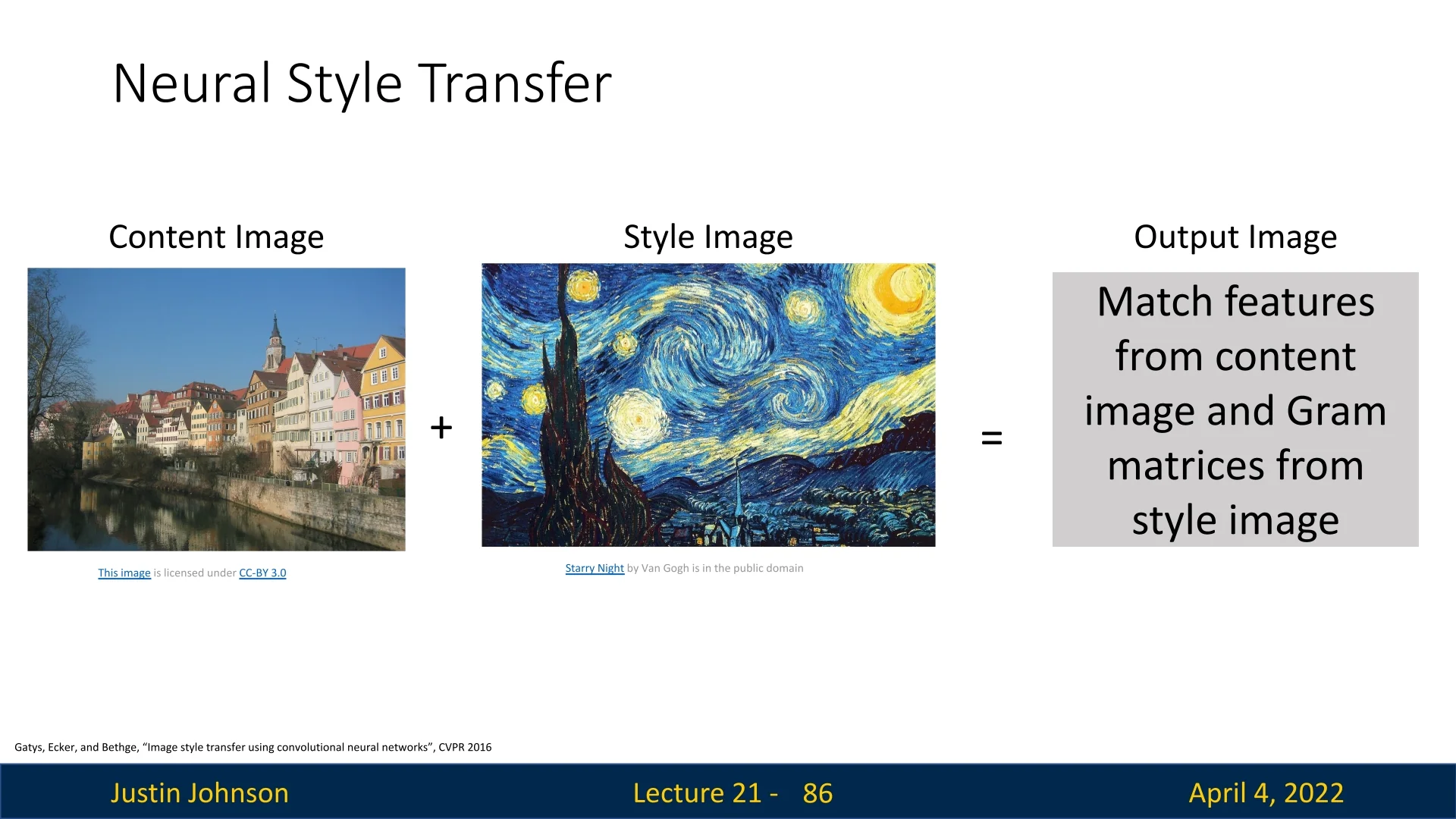
21.12 Neural Style Transfer
21.12.1 Neural Style Transfer: Content and Style Fusion
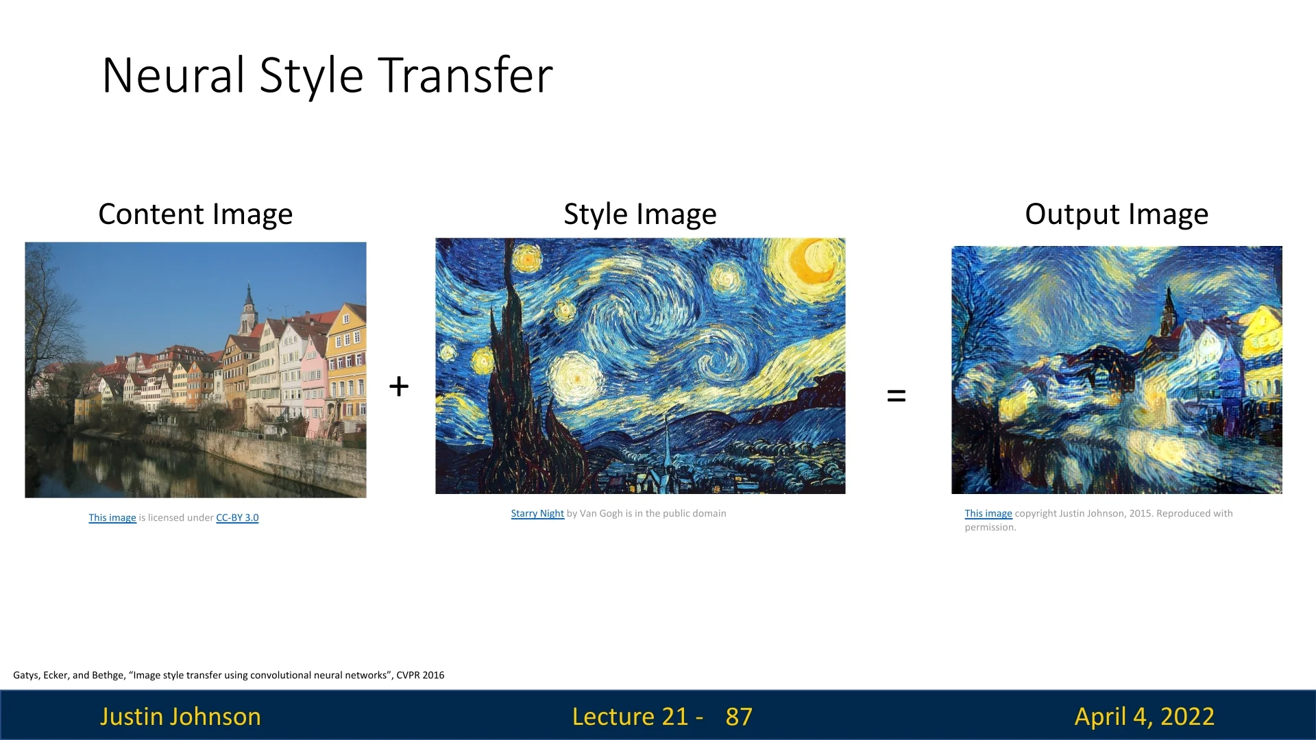
Neural Style Transfer (NST) generates a new image \( I^{\ast } \) that merges the semantic content of one image with the visual style of another. Drawing from advances in texture synthesis and feature inversion, NST formulates an optimization problem over a pre-trained convolutional network (typically VGG-19), where the goal is to make \( I^{\ast } \) simultaneously match:
- The content features of a content image \( I_c \), extracted from higher-level activations.
- The style statistics of a style image \( I_s \), encoded as Gram matrices across multiple layers.
Intuition Deep convolutional layers capture high-level abstractions—such as objects and layout—while shallow layers encode texture, edges, and color patterns. NST leverages this hierarchy by aligning \( I^{\ast } \)’s deep activations with \( I_c \)’s to preserve structure, and matching Gram matrices at multiple depths to reflect \( I_s \)’s stylistic patterns. This allows content and style to be fused in a perceptually coherent manner.
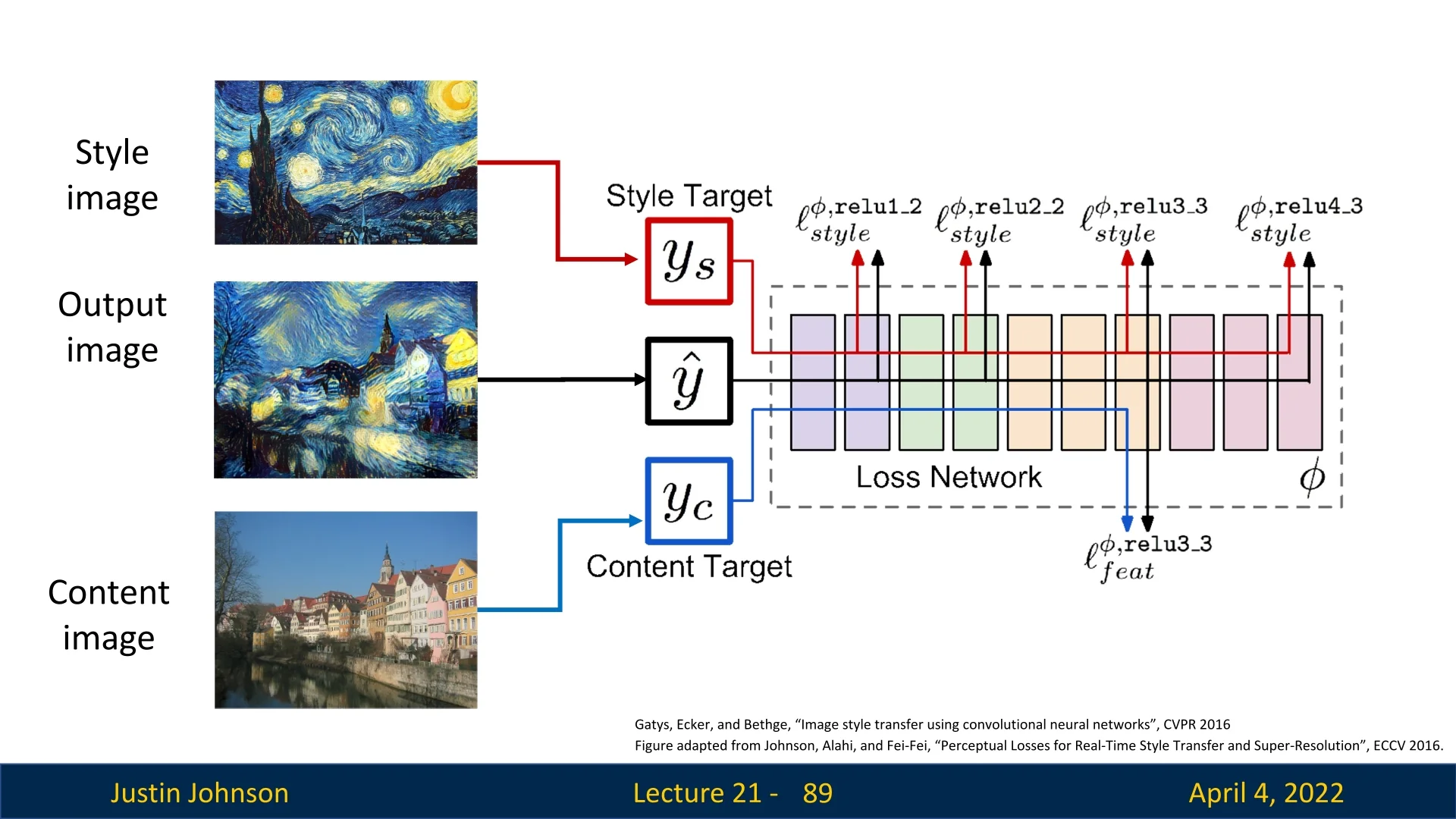
Optimization Objective The network acts as a fixed perceptual encoder. To synthesize \( I^{\ast } \), we minimize a loss combining:
- Content loss: Encourages \( I^{\ast } \) to replicate the activations of \( I_c \) at a deep layer (e.g., conv4_2), capturing object identity and layout.
- Style loss: Encourages \( I^{\ast } \) to match the Gram matrices of \( I_s \) across several layers (e.g., conv1_1 to conv5_1), encoding texture statistics at multiple spatial scales.
These losses are defined over the same network, so inputs must be compatible in resolution. Although Gram matrices are spatially invariant—aggregating across spatial locations—it is standard practice to resize \( I_c \), \( I_s \), and \( I^{\ast } \) to a common resolution for stable optimization and fair comparison of content and style representations.
Together, this dual-objective framework enables the creation of images that preserve the global structure of a scene while adopting the local visual patterns of a target artistic style.
Optimization via Gradient Descent To find the stylized image \( I^{\ast } \), we define a total loss function that balances content fidelity and style transfer: \[ \mathcal {L}_{\mbox{total}}(I^{\ast }) = \alpha \cdot \mathcal {L}_{\mbox{content}}(I^{\ast }, I_c) + \beta \cdot \mathcal {L}_{\mbox{style}}(I^{\ast }, I_s) \] where:
- Content Loss: \[ \mathcal {L}_{\mbox{content}}(I^{\ast }, I_c) = \left \| \phi _\ell (I^{\ast }) - \phi _\ell (I_c) \right \|_2^2 \] This term ensures that the synthesized image \( I^{\ast } \) matches the content features of \( I_c \) at a chosen higher layer \( \ell \) of the CNN. The function \( \phi _\ell (\cdot ) \) denotes the activations at layer \( \ell \), which encode abstract structural and semantic information.
- Style Loss: \[ \mathcal {L}_{\mbox{style}}(I^{\ast }, I_s) = \sum _j w_j \cdot \left \| G^j(I^{\ast }) - G^j(I_s) \right \|_F^2 \] This term measures the difference in style between \( I^{\ast } \) and \( I_s \) by comparing their Gram matrices \( G^j(\cdot ) \) at multiple layers \( j \). Each Gram matrix captures the pairwise correlations between feature channels, reflecting texture and visual style. The weights \( w_j \) control the relative importance of style matching across layers.
The optimization starts from a randomly initialized image—or optionally the content image itself—and iteratively updates the pixels of \( I^{\ast } \) using gradient descent. In each iteration:
- 1.
- \( I^{\ast } \) is passed through the CNN to extract content and style features.
- 2.
- The total loss \( \mathcal {L}_{\mbox{total}} \) is computed.
- 3.
- Gradients of this loss with respect to the image \( I^{\ast } \) are computed via backpropagation.
- 4.
- The image is updated to reduce the loss: \( I^{\ast } \gets I^{\ast } - \eta \cdot \nabla _{I^{\ast }} \mathcal {L}_{\mbox{total}} \), where \( \eta \) is the learning rate.
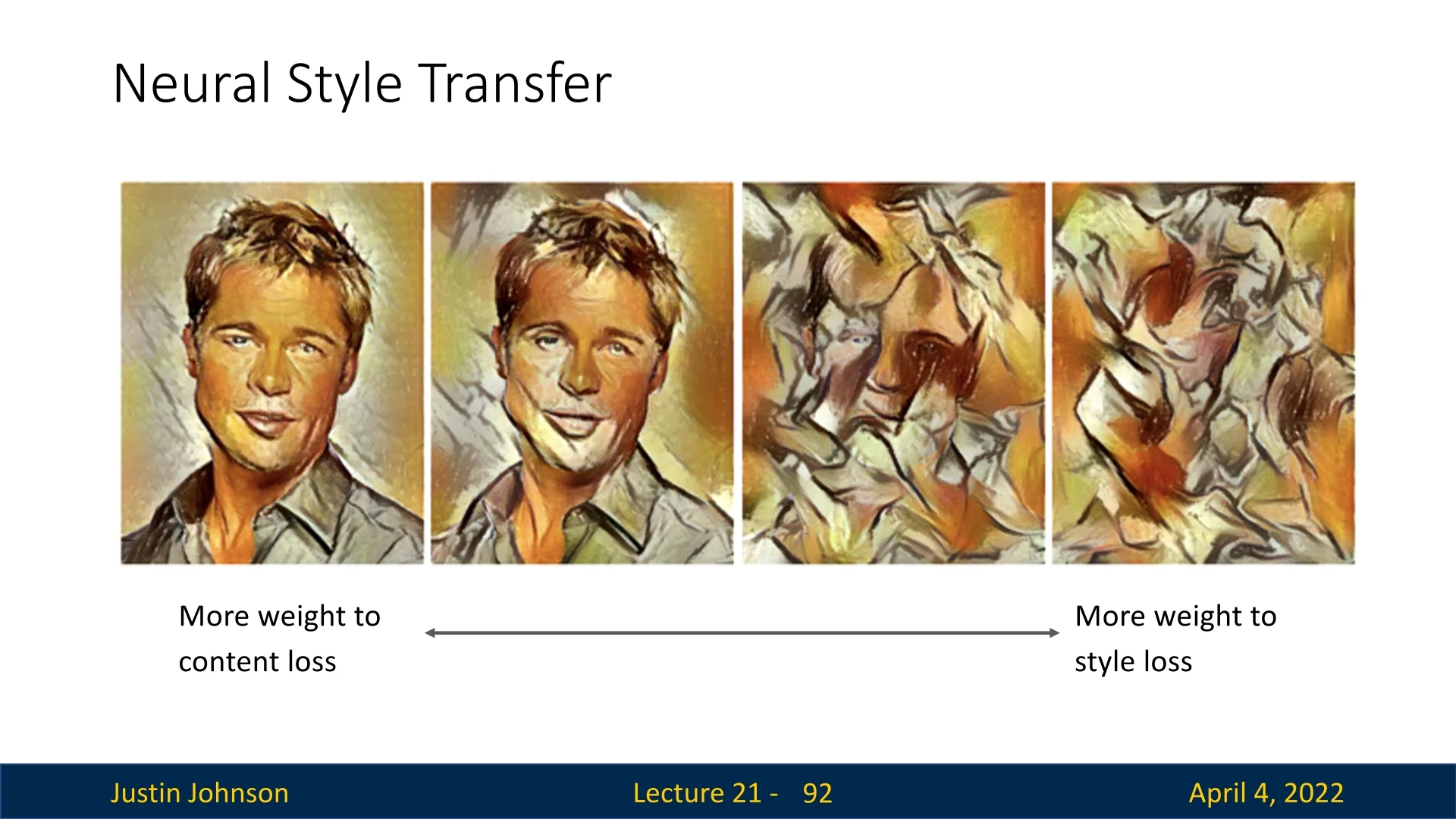
The trade-off parameters \( \alpha \) and \( \beta \) modulate the relative emphasis on content preservation versus style transfer. A higher \( \alpha / \beta \) ratio favors structural fidelity, while a lower ratio prioritizes stylization. This balance enables the method to flexibly interpolate between photorealistic and painterly outputs.
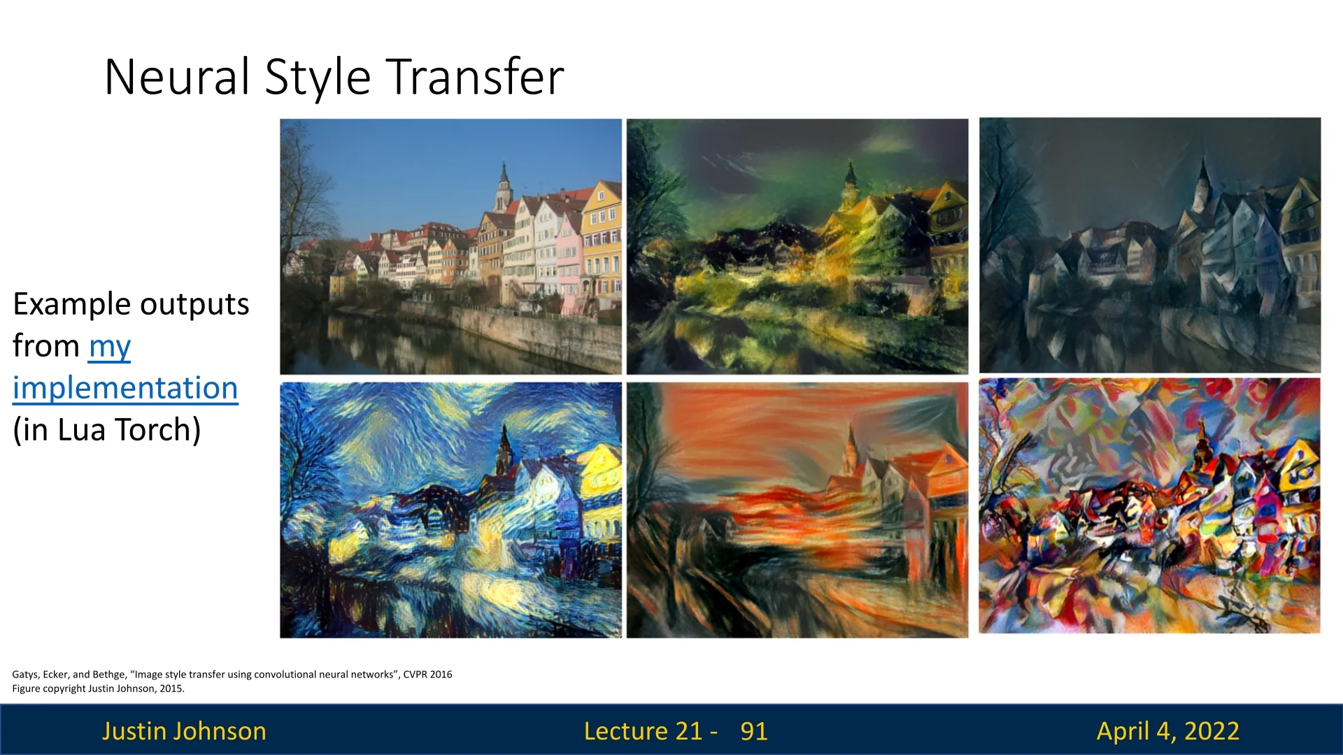
Stylization Results The outcome of this optimization is a new image that visually blends the spatial layout of the content image with the textures and patterns of the style image.
Controlling Style Intensity Adjusting the ratio \( \beta / \alpha \) enables control over how strongly the style is imposed versus how much content is preserved.
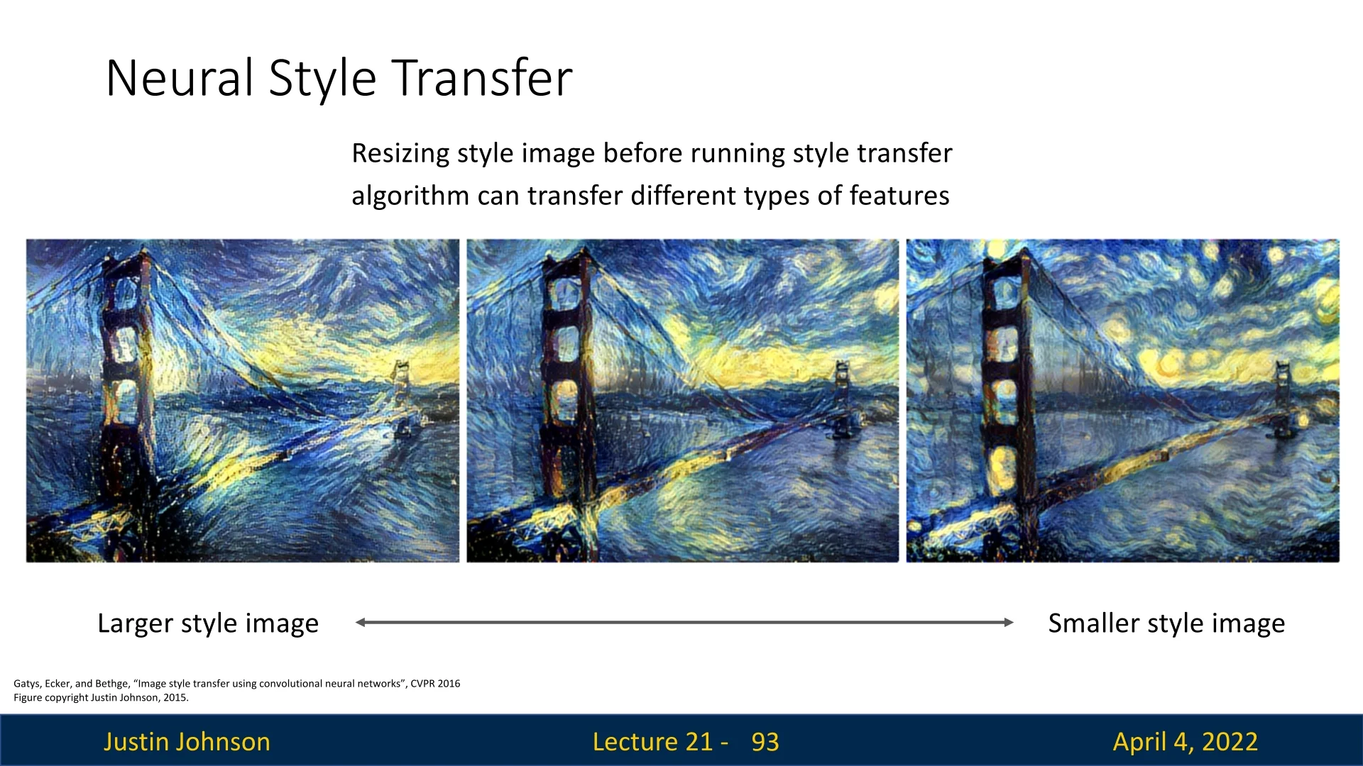
Effect of Style Image Scale Interestingly, the spatial scale of the style image affects the type of features that are transferred. Large style images encourage local brushstrokes; small images bias the transfer toward large-scale visual motifs.
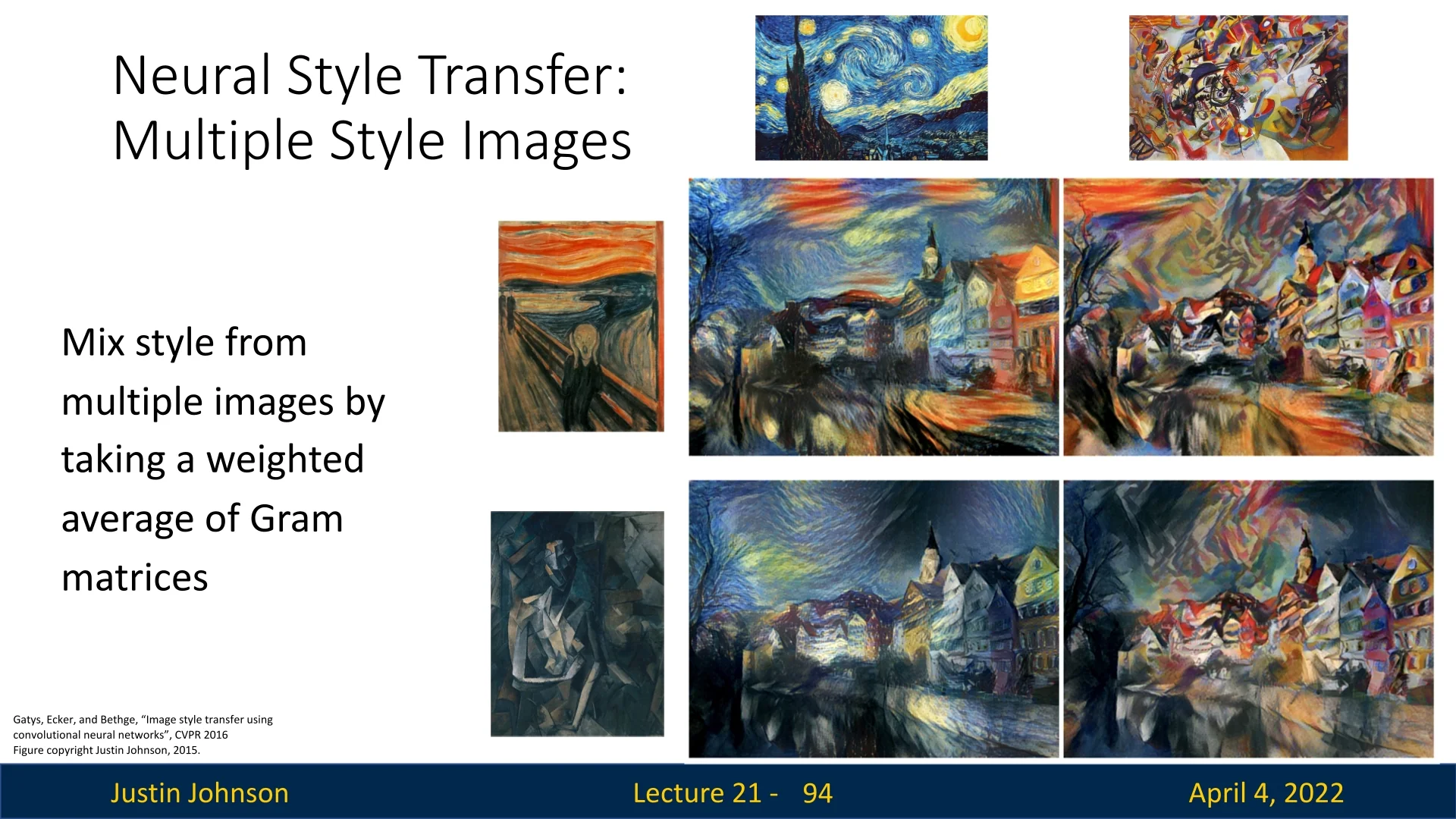
Combining Styles Neural Style Transfer can be extended to blend multiple styles by mixing the corresponding Gram matrices: \[ \mathcal {L}_{\mbox{style}}^{\mbox{combined}} = \gamma \cdot \mathcal {L}_{\mbox{style}}^{(1)} + (1 - \gamma ) \cdot \mathcal {L}_{\mbox{style}}^{(2)} \] This enables generation of novel, hybrid artistic effects.
Limitations Despite its effectiveness, this method is computationally expensive—each new stylized image requires many forward and backward passes through the CNN. This limitation motivates the development of real-time methods, discussed next.
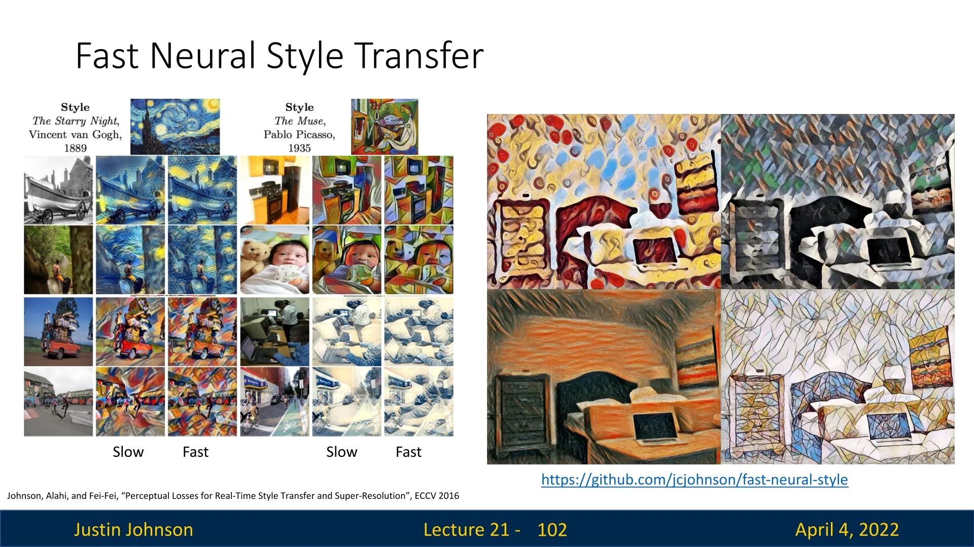
21.12.2 Fast Neural Style Transfer
While the original Neural Style Transfer algorithm produces compelling results, its reliance on iterative optimization makes it computationally expensive. Each stylized image requires dozens to hundreds of forward and backward passes through a deep network (e.g., VGG-19), making real-time applications infeasible.
To address this limitation, Johnson et al. [279] proposed an alternative: train a separate feedforward neural network to perform style transfer in a single forward pass. Once trained, this network can stylize new content images extremely efficiently—enabling real-time inference.
Training Setup The core idea is to use the same perceptual loss as before—combining content and style objectives—but apply it to train the weights of a stylization network \( T_\theta (\cdot ) \) rather than directly optimizing the image pixels.
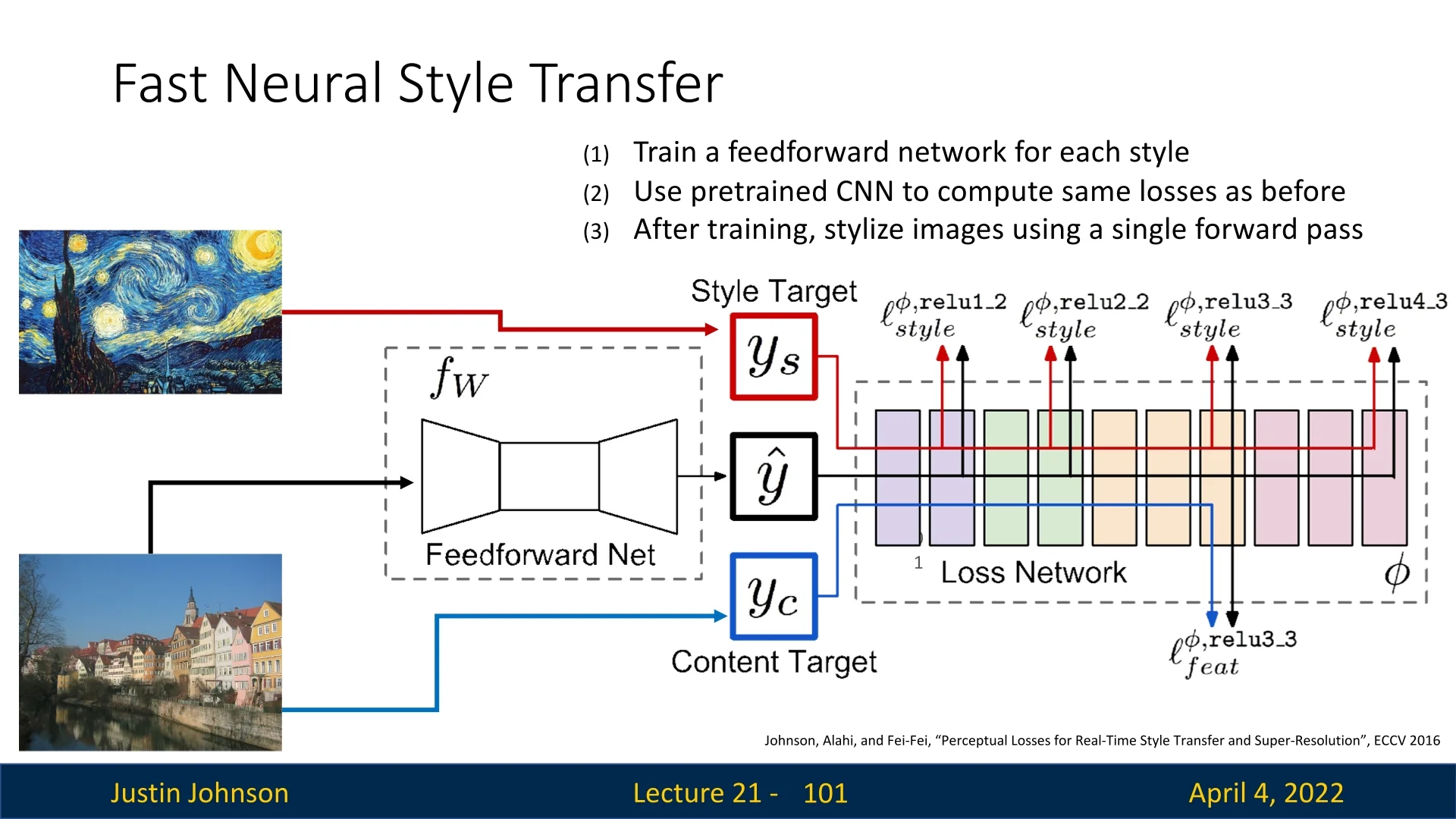
Key Insight Instead of solving: \[ \arg \min _I \; \mathcal {L}_{\mbox{content}}(I, I_c) + \mathcal {L}_{\mbox{style}}(I, I_s) \] for each new image \( I_c \), the fast method learns: \[ \arg \min _\theta \; \mathbb {E}_{I_c} \left [ \mathcal {L}_{\mbox{content}}(T_\theta (I_c), I_c) + \mathcal {L}_{\mbox{style}}(T_\theta (I_c), I_s) \right ] \] This way, the trained network \( T_\theta \) can stylize any new image without additional optimization.
Stylization Examples Once trained, the feedforward network can apply the desired style instantly.
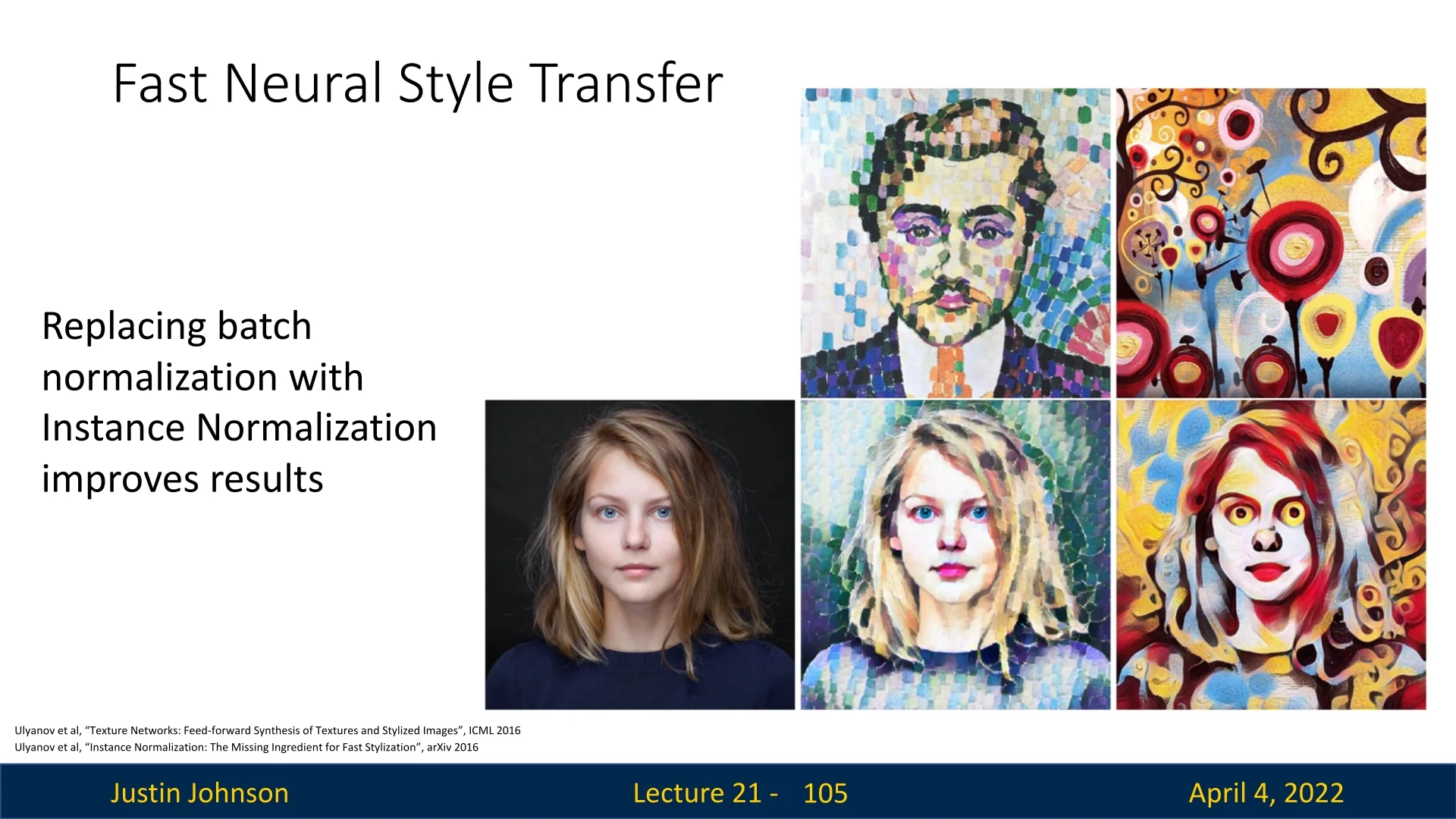
Instance Normalization Ulyanov et al. [660] discovered that replacing batch normalization with instance normalization significantly improves stylization quality. Unlike batch norm, instance norm normalizes each feature map independently for each image—preserving per-instance feature statistics critical for style representation.
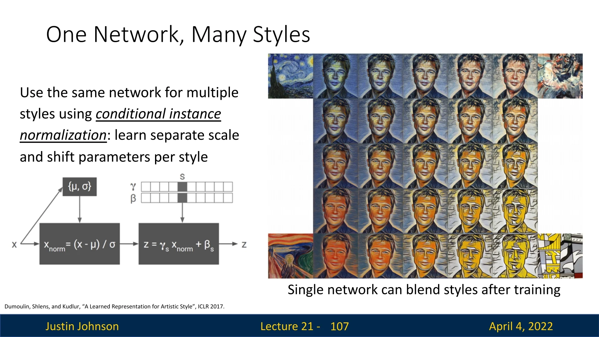
Conditional Instance Normalization for Multi-Style Transfer Training one network per style is inefficient. Dumoulin et al. [137] introduced conditional instance normalization, allowing a single network to stylize multiple styles. Each style is associated with a unique set of scale and shift parameters: \[ \mbox{IN}(x; s) = \gamma ^{(s)} \cdot \frac {x - \mu }{\sigma } + \beta ^{(s)} \] where \( s \) denotes the selected style and \( (\gamma ^{(s)}, \beta ^{(s)}) \) are learned per style. This allows:
- Fast switching between styles within one model.
- Style interpolation via blending parameters.
Summary and Emerging Directions Fast neural style transfer leverages perceptual losses to train a feedforward network that efficiently stylizes images in real time—an elegant engineering solution bridging artistic quality and speed. However, this paradigm is now being extended further by cutting-edge approaches:
- Diffusion Model Style Transfer: Recent work such as DiffeseST introduces training-free style transfer using diffusion models, leveraging DDIM inversion and spatial-textual embeddings to achieve high-fidelity stylization without per-image optimization [249].
- Self-Supervised Style Augmentation: SASSL uses neural style transfer as a data augmentation technique in self-supervised learning, improving representation quality by enhancing style diversity while preserving content semantics [547].
- Semantically-Guided Diffusion Stylization: Models like StyleDiffusion and InST apply diffusion processes with adaptive conditioning to disentangle style and content features, offering richer control in stylization [708, 803].
These advances demonstrate the ongoing evolution of style transfer—incorporating generative modeling, efficient adaptation, and semantic awareness—which promise more powerful and flexible tools in future editions of this textbook.