Lecture 20: Generative Models II
20.1 VAE Training and Data Generation
In the previous chapter, we introduced the Evidence Lower Bound (ELBO) as a tractable surrogate objective for training latent variable models. We now dive deeper into how this lower bound is used in practice, detailing each component of the architecture and training pipeline.
20.1.1 Encoder and Decoder Architecture: MNIST Example
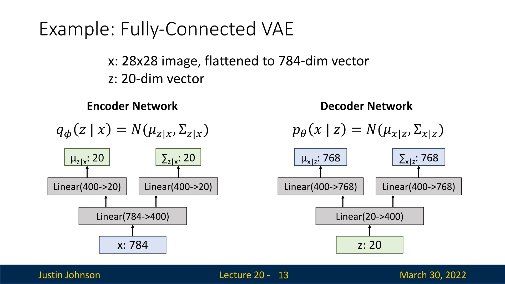
Consider training a VAE on the MNIST dataset. Each MNIST image is \(28 \times 28\) grayscale, flattened into a 784-dimensional vector \( \mathbf {x} \in \mathbb {R}^{784} \). We choose a 20-dimensional latent space \( \mathbf {z} \in \mathbb {R}^{20} \).
20.1.2 Training Pipeline: Step-by-Step
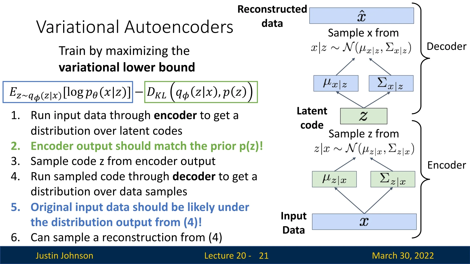
The ELBO Objective Recall from our theoretical derivation that our ultimate goal is to maximize the marginal log-likelihood of the data, \(\log p_\theta (\mathbf {x})\). However, computing this probability directly involves an intractable integral over the high-dimensional latent space. To circumvent this, we maximize a tractable surrogate objective known as the Evidence Lower Bound (ELBO):
\begin {equation} \log p_\theta (\mathbf {x}) \geq \underbrace {\mathbb {E}_{\mathbf {z} \sim q_\phi (\mathbf {z} \mid \mathbf {x})} \left [ \log p_\theta (\mathbf {x} \mid \mathbf {z}) \right ]}_{\mbox{reconstruction term}} - \underbrace {D_{\mathrm {KL}} \left (q_\phi (\mathbf {z} \mid \mathbf {x}) \,\|\, p(\mathbf {z}) \right )}_{\mbox{KL regularization}}. \label {eq:chapter20_elbo} \end {equation}
We train two neural networks simultaneously—the encoder (inference network) and the decoder (generative network)—to maximize this lower bound. Since standard deep learning frameworks (like PyTorch or TensorFlow) are designed to minimize loss functions, we formally define the VAE Loss as the negative ELBO: \begin {equation} \mathcal {L}_{\mbox{VAE}} = - \mbox{ELBO}. \label {eq:chapter20_vae_loss_def} \end {equation}
Crucial nuance: Minimizing this loss is not strictly equivalent to maximizing the true data likelihood. We are optimizing a lower bound. The gap between the log-likelihood and the ELBO is exactly the expected KL divergence between our approximate posterior and the true posterior, \(\log p_\theta (\mathbf {x}) - \mbox{ELBO} = \mathbb {E}_{\mathbf {x} \sim p_{\mbox{data}}} \left [ D_{\mathrm {KL}}\big (q_\phi (\mathbf {z} \mid \mathbf {x}) \,\|\, p_\theta (\mathbf {z} \mid \mathbf {x})\big ) \right ]\). If the encoder is not expressive enough to match the true posterior, this gap remains strictly positive. This fundamental limitation—optimizing a bound rather than the exact marginal likelihood—is one reason why later generative model families, such as diffusion models and flow-based models, explore alternative training objectives that do not rely on variational lower bounds.
For a high-level discussion on the properties of latent spaces (e.g., the manifold hypothesis), please refer back to Section Lecture 19 (Chapter 19). Below, we detail the practical execution of the VAE training pipeline in six stages.
- 1.
- Run input \( \mathbf {x} \) through the encoder.
The encoder network \( q_\phi (\mathbf {z} \mid \mathbf {x}) \) processes the input image, but unlike a standard autoencoder, it does not output a single latent code. Instead, it predicts a probability distribution over the latent space. Specifically, for a latent dimensionality \( J \), the encoder outputs two vectors: \[ \boldsymbol {\mu }_{z|x} \in \mathbb {R}^J \quad \mbox{and} \quad \boldsymbol {\sigma }^2_{z|x} \in \mathbb {R}^J \] These vectors parameterize a diagonal Gaussian distribution \( q_\phi (\mathbf {z} \mid \mathbf {x}) = \mathcal {N}(\boldsymbol {\mu }_{z|x}, \operatorname {diag}(\boldsymbol {\sigma }^2_{z|x})) \). In what follows, we will often abbreviate \(\boldsymbol {\mu }_{z|x}\) and \(\boldsymbol {\sigma }^2_{z|x}\) as \(\boldsymbol {\mu }\) and \(\boldsymbol {\sigma }^2\) for brevity.
Note on Stability: In many implementations, the encoder actually predicts log-variance, \(\log \boldsymbol {\sigma }^2\), rather than \(\boldsymbol {\sigma }^2\) directly. This improves numerical stability by mapping the variance domain \((0, \infty )\) to the real line \((-\infty , \infty )\). The variance is then recovered via an element-wise exponential.
- 2.
- Compute the KL divergence between the encoder’s
distribution and the prior.
To ensure the latent space remains well-behaved, we enforce a penalty if the encoder’s predicted distribution diverges from a fixed prior, typically the standard multivariate Gaussian \( p(\mathbf {z}) = \mathcal {N}(\mathbf {0}, \mathbf {I}) \).
Because both the posterior and prior are Gaussian, the Kullback-Leibler (KL) divergence has a convenient closed-form solution. We compute this simply by summing over all \( J \) latent dimensions: \begin {equation} D_{\mathrm {KL}}\big (q_\phi (\mathbf {z} \mid \mathbf {x}) \,\|\, p(\mathbf {z})\big ) = \frac {1}{2} \sum _{j=1}^{J} \left ( 1 + \log \sigma _j^2 - \mu _j^2 - \sigma _j^2 \right ). \label {eq:chapter20_vae_kl_closed_form} \end {equation} This term acts as a regularizer. It pulls the mean \( \boldsymbol {\mu } \) towards 0 and the variance \( \boldsymbol {\sigma }^2 \) towards 1. Without this term, the encoder could ”cheat” by clustering data points far apart (making \( \mu \) huge) or by shrinking the variance to effectively zero (making \( \sigma \to 0 \)), effectively collapsing the VAE back into a standard deterministic autoencoder.
- 3.
- Sample latent code \( \mathbf {z} \) using the Reparameterization Trick.
The decoder requires a concrete vector \( \mathbf {z} \) to generate an output. Therefore, we must sample from the distribution defined by \( \boldsymbol {\mu } \) and \( \boldsymbol {\sigma } \).
The Obstacle (Blocking Gradients): A naive sampling operation breaks the computation graph. Backpropagation requires continuous derivatives, but we cannot differentiate with respect to a random roll of the dice. If we simply sampled \( z \), the gradient flow would stop at the sampling node.
The Solution (Reparameterization): We use the reparameterization trick to bypass this block. We express \( \mathbf {z} \) as a deterministic transformation of the encoder parameters and an auxiliary noise source: \begin {equation} \mathbf {z} = \boldsymbol {\mu }_{z|x} + \boldsymbol {\sigma }_{z|x} \odot \boldsymbol {\epsilon }, \quad \boldsymbol {\epsilon } \sim \mathcal {N}(\mathbf {0}, \mathbf {I}). \label {eq:chapter20_vae_reparameterization} \end {equation} Practical Implementation Details:
- Source of Randomness: We sample a noise vector \(\boldsymbol {\epsilon } \in \mathbb {R}^J\) from \(\mathcal {N}(\mathbf {0}, \mathbf {I})\). This variable effectively ”holds” the stochasticity.
- Vectorization: In practice, we sample a unique \( \boldsymbol {\epsilon } \) for every data point in the batch during every forward pass.
- Gradient Flow: The operation \( \odot \) denotes element-wise multiplication. Crucially, because \( \boldsymbol {\epsilon } \) is treated as an external constant during the backward pass, gradients can flow freely through \( \boldsymbol {\mu } \) and \( \boldsymbol {\sigma } \) back to the encoder weights.
For a visual walkthrough of this mechanism, we recommend:
ML&DL Explained { Reparameterization Trick. - 4.
- Feed the sampled latent code \( \mathbf {z} \) into the decoder.
The decoder \( p_\theta (\mathbf {x} \mid \mathbf {z}) \) maps the sampled code \( \mathbf {z} \) back to the high-dimensional data space. It outputs the parameters of the likelihood distribution for the pixels (e.g., the predicted mean intensity for each pixel).
- 5.
- Evaluate the reconstruction likelihood.
We measure how well the decoder ”explains” the original input \( \mathbf {x} \) given the sampled code \( \mathbf {z} \). For real-valued images, we typically assume a factorized Gaussian likelihood with fixed variance. In this case, maximizing the log-likelihood is equivalent (up to an additive constant) to minimizing the squared \(\ell _2\) reconstruction error: \begin {equation} \mathcal {L}_{\mbox{recon}} \,\propto \, \left \| \mathbf {x} - \hat {\mathbf {x}} \right \|_2^2. \label {eq:chapter20_vae_recon_mse} \end {equation}
- 6.
- Combine terms to compute the total VAE Loss.
The final objective function is the sum of the reconstruction error and the regularization penalty: \begin {equation} \mathcal {L}_{\mbox{VAE}}(\mathbf {x}) = \underbrace {- \mathbb {E}_{\mathbf {z} \sim q_\phi (\mathbf {z} \mid \mathbf {x})} \left [\log p_\theta (\mathbf {x} \mid \mathbf {z})\right ]}_{\mbox{reconstruction loss}} + \underbrace {D_{\mathrm {KL}}\big (q_\phi (\mathbf {z} \mid \mathbf {x}) \,\|\, p(\mathbf {z})\big )}_{\mbox{regularization loss}}. \label {eq:chapter20_vae_total_loss} \end {equation}
The VAE “Tug-of-War” (Regularization vs. Reconstruction):
The VAE objective function creates a fundamental conflict between two opposing goals, forcing the model to find a useful compromise:
- The Reconstruction Term (Distinctness):
-
This term maximizes \(\mathbb {E}[\log p_\theta (\mathbf {x} \mid \mathbf {z})]\). It drives the encoder to be as precise as possible to minimize error. The Extreme Case: If left unchecked, the encoder would reduce the variance to zero (\(\sigma \to 0\)). The latent distribution would collapse into a Dirac delta function (a single point), effectively turning the VAE into a standard deterministic Autoencoder. While this minimizes reconstruction error, the model effectively “memorizes” the training data as isolated points, failing to learn the smooth, continuous manifold required for generating new images.
- The KL Term (Smoothness):
-
This term minimizes \(D_{\mathrm {KL}}(q_\phi (\mathbf {z} \mid \mathbf {x}) \,\|\, p(\mathbf {z}))\). It forces the encoder’s output to match the standard Gaussian prior (\(\mathcal {N}(0, I)\)), encouraging posteriors to be “noisy” and overlap. The Extreme Case: If left unchecked (i.e., if this regularization dominates), the encoder will ignore the input \(\mathbf {x}\) entirely to satisfy the prior perfectly. This phenomenon, known as Posterior Collapse, results in latent codes that contain no information about the input image, causing the decoder to output generic noise or average features regardless of the input.
The Result: This tension prevents the model from memorizing exact coordinates (Autoencoder) while preventing it from outputting pure noise (Posterior Collapse). The VAE settles on a “cloud-like” representation that is distinct enough to preserve content but smooth enough to allow for interpolation and generation.
Why a Diagonal Gaussian Prior?
We typically choose the prior \( p(\mathbf {z}) \) to be a unit Gaussian \( \mathcal {N}(\mathbf {0}, \mathbf {I}) \). While simple, this choice provides powerful benefits:
- Analytical Tractability: As seen in Equation 20.3, the KL divergence between two Gaussians can be computed without expensive sampling or integrals.
- Encouraging Disentanglement: The diagonal covariance structure assumes independence between dimensions. This biases the model towards allocating distinct generative factors to separate dimensions (e.g., “azimuth” vs. “elevation”) rather than entangling them, although in practice such disentanglement is not guaranteed.
- Manifold Smoothness: By forcing the posterior to overlap with the standard normal prior, we prevent the model from memorizing the training set (which would look like a set of isolated delta functions). Instead, the model learns a smooth, continuous manifold where any point sampled from \( \mathcal {N}(\mathbf {0}, \mathbf {I}) \) is likely to decode into a plausible image.
20.1.3 How Can We Generate Data Using VAEs?
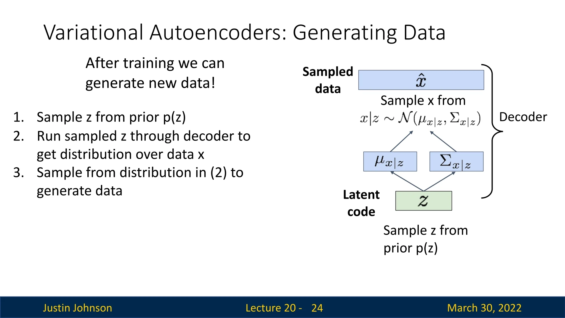
Once a Variational Autoencoder is trained, we can use it as a generative model to produce new data samples. Unlike the training phase, which starts from observed inputs \( \mathbf {x} \), the generative process starts from the latent space.
Sampling Procedure To generate a new data point (e.g., a novel image), we follow a simple three-step process:
- 1.
- Sample a latent code \( \mathbf {z} \sim p(\mathbf {z}) \).
This draws from the prior distribution, which is typically set to \( \mathcal {N}(\mathbf {0}, \mathbf {I}) \). The latent space has been trained such that this prior corresponds to plausible latent factors of variation. - 2.
- Run the sampled \( \mathbf {z} \) through the decoder \( p_\theta (\mathbf {x} \mid \mathbf {z}) \).
This yields the parameters (e.g., mean and variance) of a probability distribution over possible images. - 3.
- Sample a new data point \( \hat {\mathbf {x}} \) from this output distribution.
Typically, we sample from the predicted Gaussian: \[ \hat {\mathbf {x}} \sim \mathcal {N}(\boldsymbol {\mu }_{x|z}, \operatorname {diag}(\boldsymbol {\sigma }^2_{x|z})) \] In some applications (e.g., grayscale image generation), one might use just the mean \( \boldsymbol {\mu }_{x|z} \) as the output.
This process enables the generation of diverse and novel data samples that resemble the training distribution, but are not copies of any specific training point.
20.2 Results and Applications of VAEs
Variational Autoencoders not only enable data generation but also support rich latent-space manipulation. Below, we summarize key empirical results and capabilities demonstrated in foundational works.
20.2.1 Qualitative Generation Results
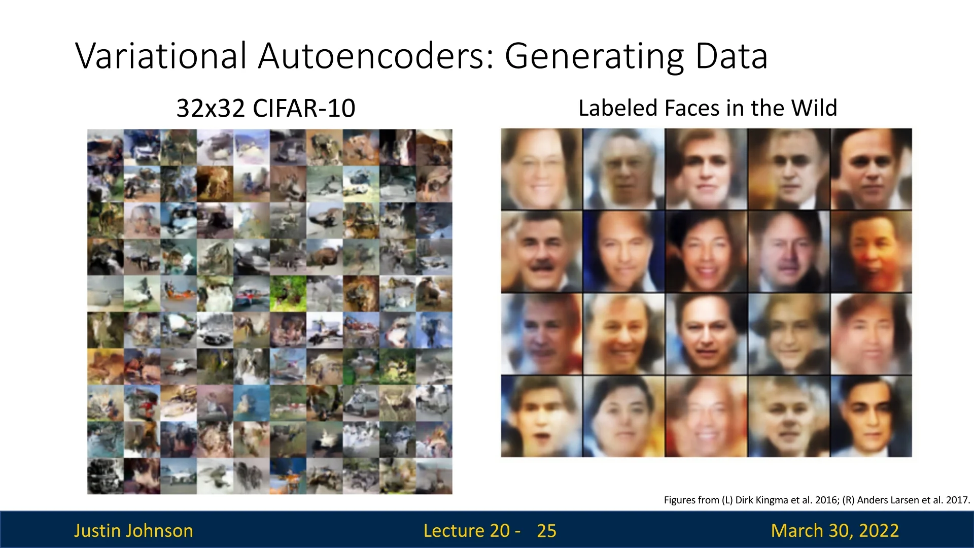
Once trained, VAEs can generate samples that resemble the training data distribution. For instance:
- On CIFAR-10, generated samples are 32×32 RGB images with recognizable textures and object-like patterns.
- On the Labeled Faces in the Wild (LFW) dataset, VAEs generate realistic human faces, capturing high-level structures such as symmetry, eyes, hair, and pose.
20.2.2 Latent Space Traversals and Image Editing
Once a VAE has been trained, we are no longer limited to simply reconstructing inputs. Because the latent prior \(p(\mathbf {z})\) is typically chosen to be a diagonal Gaussian, the model assumes that different coordinates of \(\mathbf {z}\) are a priori independent. This structural assumption makes it natural to manipulate individual latent dimensions and observe how specific changes in the code \(\mathbf {z}\) manifest in the generated data.
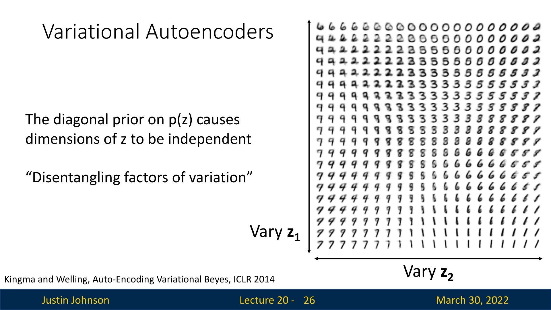
Example 1: MNIST Morphing A classic illustration of this property is provided by [304] using the MNIST dataset of handwritten digits. By training a VAE with a strictly two-dimensional latent space, we can visualize the learned manifold by systematically varying the latent variables \( z_1 \) and \( z_2 \) across a regular grid (using the inverse CDF of the Gaussian to map the grid to probability mass) and decoding the results.
As shown in the below figure, this reveals a highly structured and continuous latent space. Rather than jumping randomly between digits, the decoder produces smooth semantic interpolations:
- Vertical Morphing (\( z_1 \)): Moving along the vertical axis transforms the digit identity smoothly. For instance, we can observe a 6 morphing into a 9, which then transitions into a 7. With slight variations in \( z_2 \), this path may also pass through a region decoding to a 2.
- Horizontal Morphing (\( z_2 \)): Moving along the horizontal axis produces different transitions. In some regions, a 7 gradually straightens into a 1. In others, a 9 thickens into an 8, loops into a 3, and settles back into an 8.
This confirms that the VAE has learned a smooth, continuous manifold where nearby latent codes decode to visually similar images, and linear interpolation in latent space corresponds to meaningful semantic morphing.
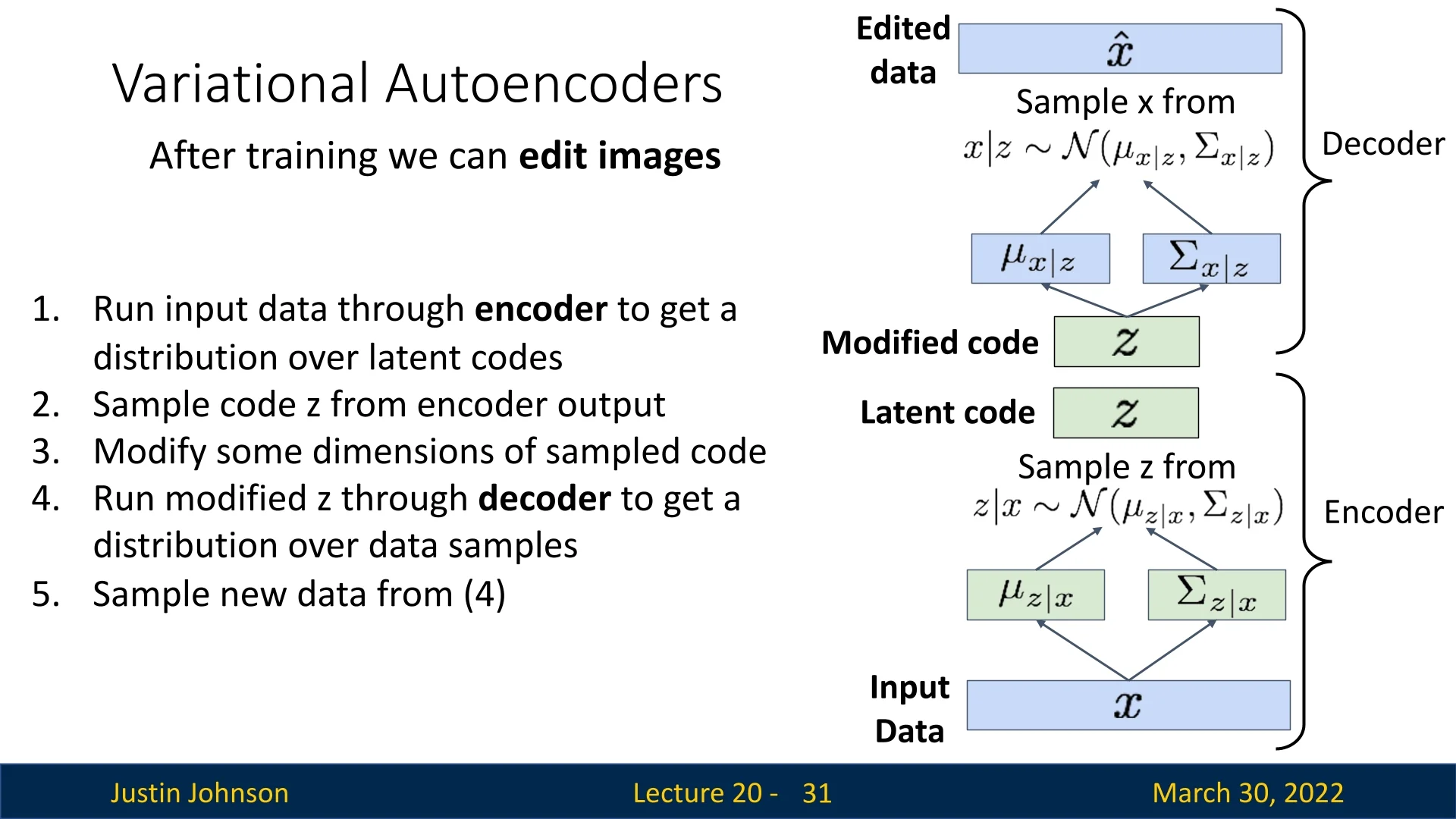
The General Editing Pipeline We can generalize this “traversal” idea into a simple but powerful pipeline for semantic image editing. As illustrated in the below figure, the process is:
- 1.
- Encode: Run the input image \( \mathbf {x} \) through the encoder to obtain the approximate posterior \( q_\phi (\mathbf {z} \mid \mathbf {x}) \).
- 2.
- Sample: Draw a latent code \( \mathbf {z} \sim q_\phi (\mathbf {z} \mid \mathbf {x}) \) using the reparameterization trick from Section 20.1.2.
- 3.
- Edit in latent space: Manually modify one or more coordinates of \( \mathbf {z} \) (for example, set \( \tilde {z}_j = z_j + \delta \)) to obtain a modified code \( \tilde {\mathbf {z}} \).
- 4.
- Decode: Pass the modified code \( \tilde {\mathbf {z}} \) through the decoder \( p_\theta (\mathbf {x} \mid \mathbf {z}) \) to obtain the parameters of an edited-image distribution \( p_\theta (\mathbf {x} \mid \tilde {\mathbf {z}}) \).
- 5.
- Visualize: Either sample \( \hat {\mathbf {x}} \sim p_\theta (\mathbf {x} \mid \tilde {\mathbf {z}}) \) or directly visualize the decoder’s mean as the edited image.
In other words, the encoder maps images to a “control space” (latent codes), we apply simple algebraic edits there, and the decoder renders the results back into image space.
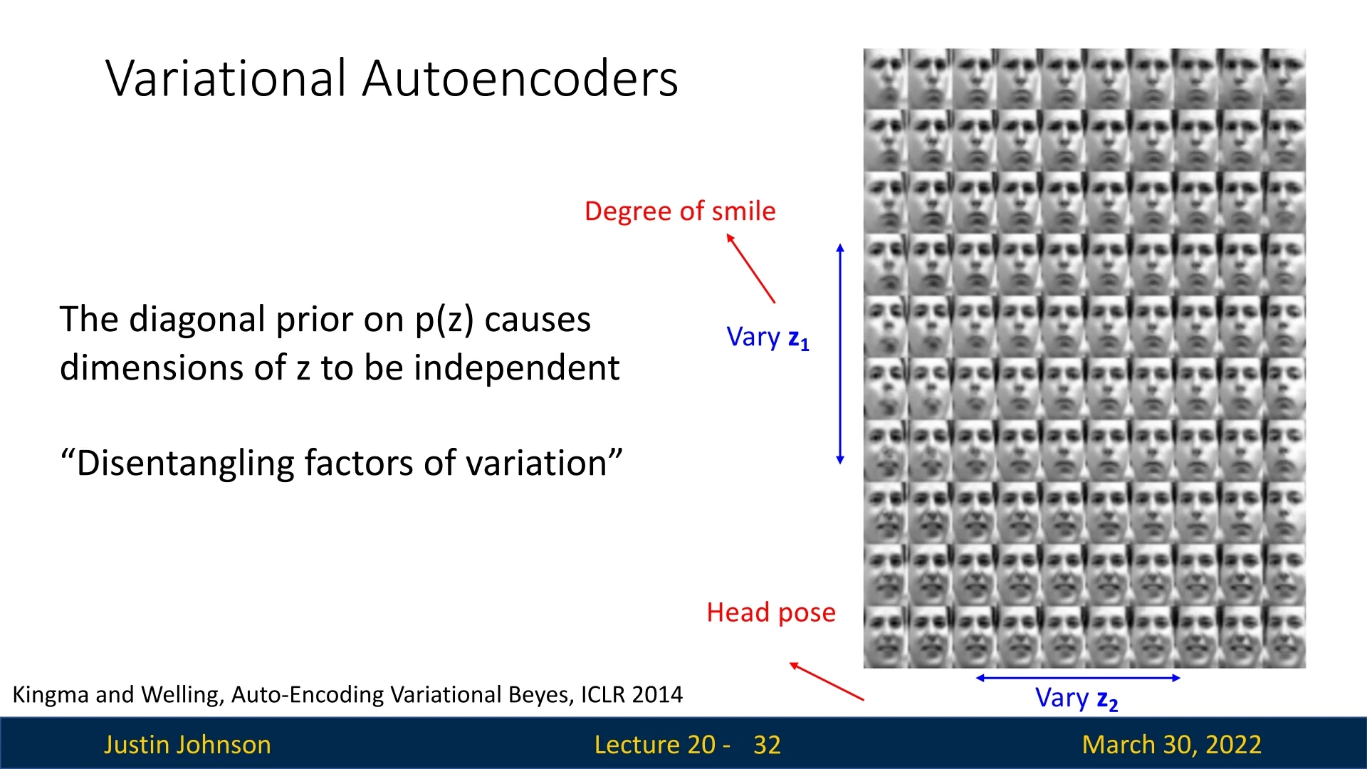
Example 2: Disentanglement in Faces While MNIST mainly exhibits simple geometric morphing, VAEs applied to more complex data often uncover high-level semantic attributes. This phenomenon is known as disentanglement: particular dimensions of \( \mathbf {z} \) align with individual generative factors.
In the original VAE paper [304], the authors demonstrated this on the Frey Face dataset. Even without label supervision, the model discovered latent coordinates that separately control expression and pose:
- Varying one latent coordinate continuously changes the degree of smiling.
- Varying another coordinate continuously changes the head pose.
This capability was further refined by [319] in the Deep Convolutional Inverse Graphics Network (DC-IGN). Training on 3D-rendered faces, they identified specific latent variables that act like “knobs” in a graphics engine:
- Pose (azimuth): rotating the head around the vertical axis while preserving identity.
- Lighting: moving the light source around the subject, while keeping pose fixed.
As shown in the following figure, editing a single latent value can rotate a face in 3D or sweep the illumination direction, indicating that the model has captured underlying 3D structure from 2D pixels.
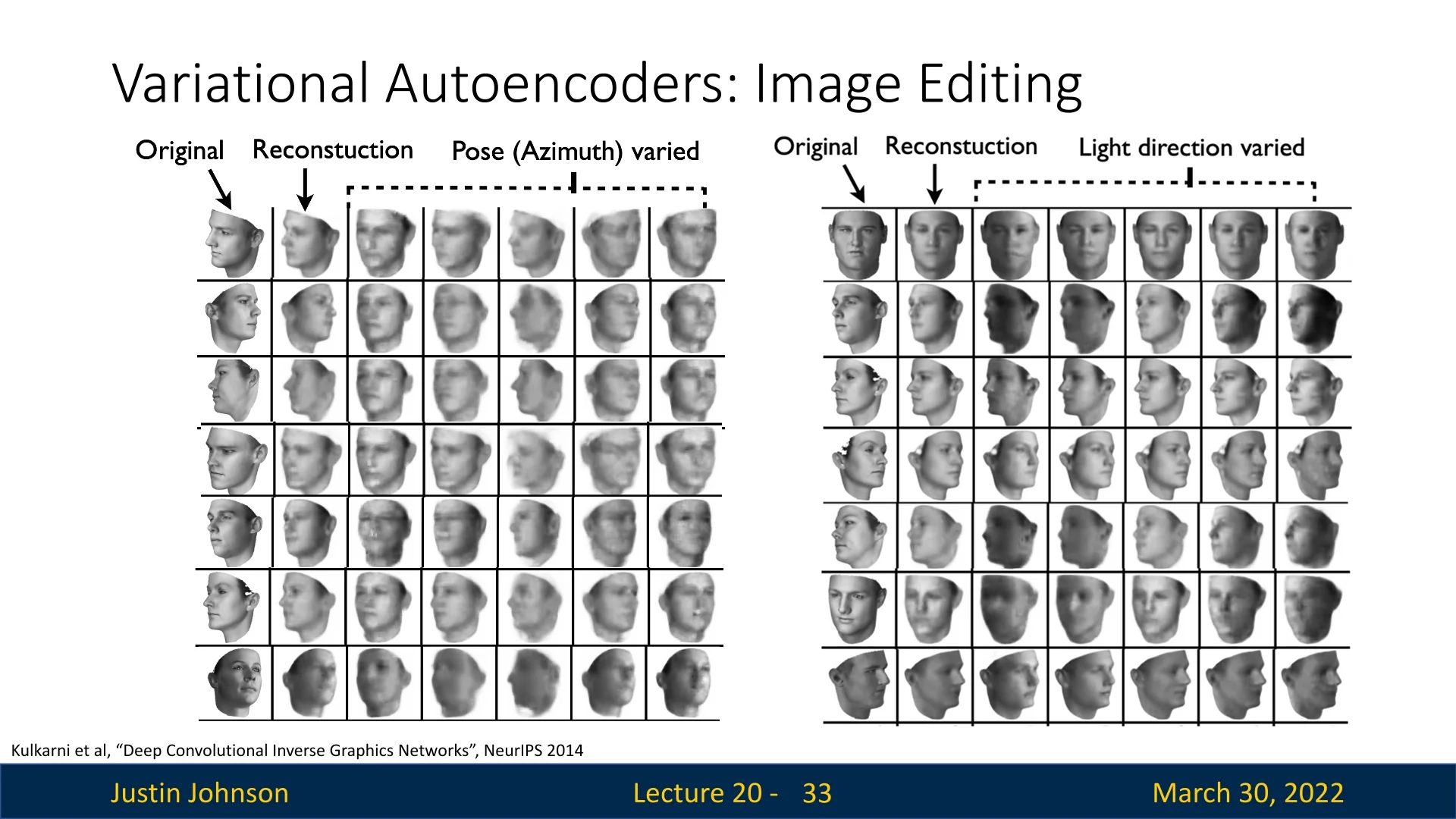
These examples highlight a key qualitative advantage of VAEs: beyond modeling the data distribution, they expose a low-dimensional latent space in which many generative factors can be probed, interpolated, and edited. In practice, disentanglement is imperfect and not guaranteed, but even partially disentangled latents already enable powerful and interpretable control over generated images.
Takeaway Unlike autoregressive models (e.g., PixelCNN) that only model \(p(\mathbf {x})\) directly and provide no explicit latent code, VAEs learn a structured latent representation \( \mathbf {z} \). This representation can be used to interpolate between images, explore variations along semantic directions, and perform targeted edits, making VAEs particularly valuable for representation learning and controllable generation.
20.3 Summary & Examples: Variational Autoencoders
Variational Autoencoders (VAEs) introduce a probabilistic framework on top of the traditional autoencoder architecture. Instead of learning a deterministic mapping, they:
- treat the latent code \( \mathbf {z} \) as a random variable drawn from an encoder-predicted posterior \( q_\phi (\mathbf {z} \mid \mathbf {x}) \),
- model the data generation process via a conditional likelihood \( p_\theta (\mathbf {x} \mid \mathbf {z}) \),
- and optimize the Evidence Lower Bound (ELBO) instead of the intractable marginal likelihood \( p_\theta (\mathbf {x}) \).
- Principled formulation: VAEs are grounded in Bayesian inference and variational methods, giving a clear probabilistic interpretation of both training and inference.
- Amortized inference: The encoder \( q_\phi (\mathbf {z} \mid \mathbf {x}) \) allows fast, single-pass inference of latent codes for new data, which can be reused for downstream tasks such as classification, clustering, or editing.
- Interpretable latent space: As seen in the traversals above, the latent space often captures semantic factors (pose, light, expression) in a smooth, continuous manifold.
- Fast sampling: Generating new data is efficient: sample \( \mathbf {z} \sim \mathcal {N}(\mathbf {0}, \mathbf {I}) \) and decode once.
- Approximation gap: VAEs maximize a lower bound (ELBO), not the exact log-likelihood. If the approximate posterior \( q_\phi (\mathbf {z} \mid \mathbf {x}) \) is too restricted (for example, diagonal Gaussian), the model may underfit and assign suboptimal likelihood to the data.
- Blurry samples: With simple factorized Gaussian decoders (and the associated MSE-like reconstruction loss), VAEs tend to produce over-smoothed images that lack the sharp, high-frequency details achieved by PixelCNNs, GANs, or diffusion models.
Active Research Directions Research on VAEs often focuses on mitigating these downsides while preserving their strengths:
- Richer posteriors: Replacing the diagonal Gaussian \( q_\phi (\mathbf {z} \mid \mathbf {x}) \) with more flexible families such as normalizing flows or autoregressive networks to reduce the ELBO gap.
- Structured priors: Using hierarchical or discrete/categorical priors and structured latent spaces to better capture factors of variation and induce disentanglement.
- Hybrid models: Combining VAEs with autoregressive decoders (e.g., PixelVAE), so that the global structure is captured by \( \mathbf {z} \) while local detail is modeled autoregressively.
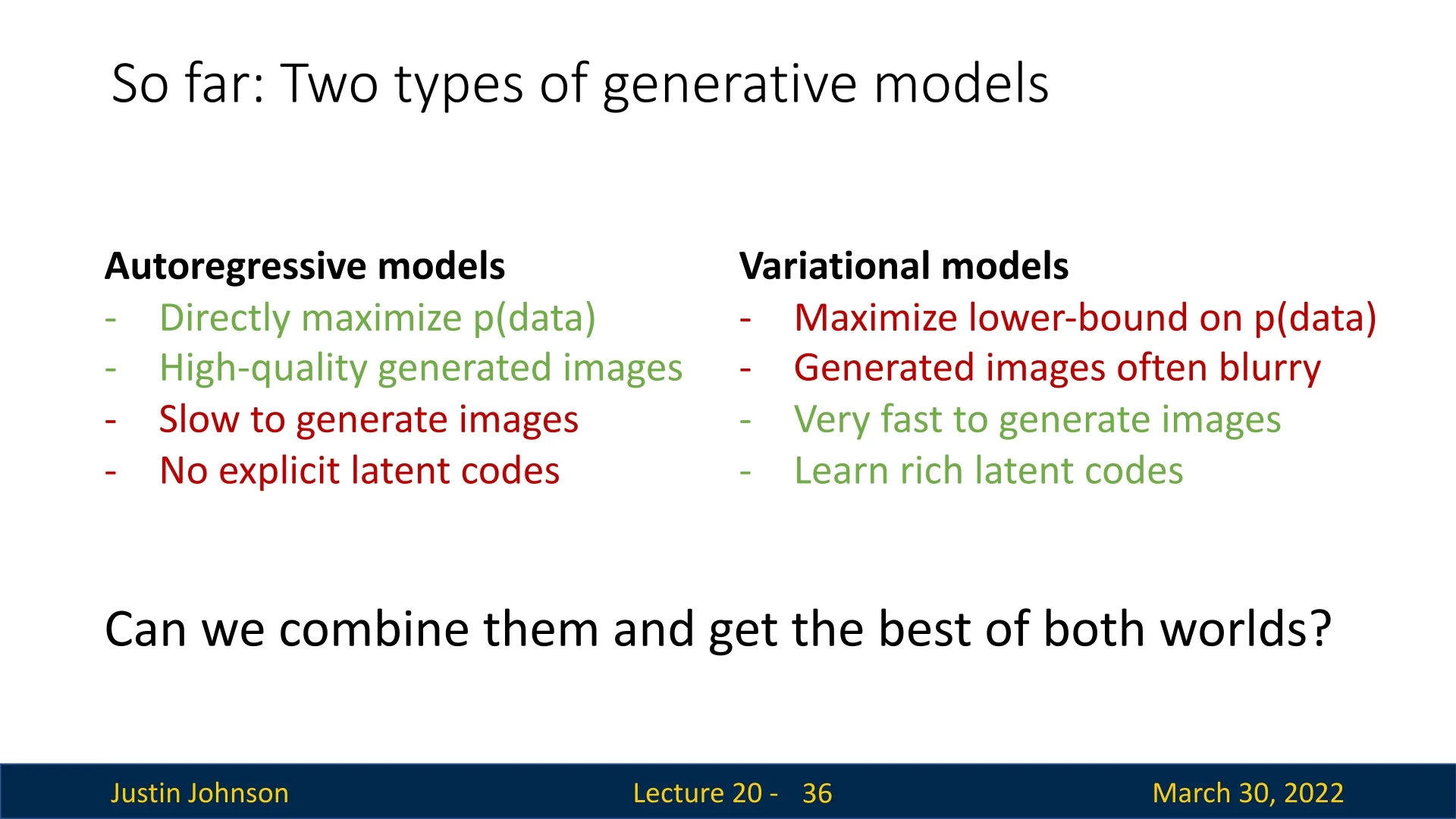
Comparison: Autoregressive vs. Variational Throughout this chapter, we have contrasted two major families of generative models. Figure 20.9 summarizes the trade-offs:
-
Autoregressive models (PixelRNN / PixelCNN):
- Directly maximize \( p_\theta (\mathbf {x}) \) with exact likelihood.
- Produce sharp, high-quality images.
- Are typically slow to sample from, since pixels are generated sequentially.
- Do not expose an explicit low-dimensional latent code.
-
Variational models (VAEs):
- Maximize a lower bound on \( p_\theta (\mathbf {x}) \) rather than the exact likelihood.
- Often produce smoother (blurrier) images with simple decoders.
- Are very fast to sample from once trained.
- Learn rich, editable latent codes that support interpolation and semantic control.
This comparison naturally raises the next question we will address: Can we combine these approaches and obtain the best of both worlds?
20.3.1 VQ-VAE-2: Combining VAEs with Autoregressive Models
Motivation Variational Autoencoders (VAEs) offer a principled latent variable framework for generative modeling, but their outputs often lack detail due to oversimplified priors and decoders. In contrast, autoregressive models such as PixelCNN produce sharp images by modeling pixel-level dependencies but lack interpretable latent variables and are slow to sample from.
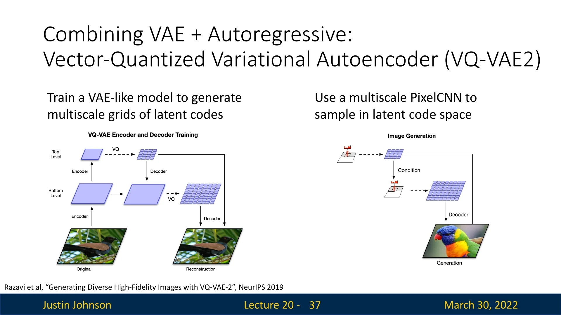
VQ-VAE-2 [530] combines these paradigms: it learns discrete latent representations via vector quantization (as in VQ-VAE), and models their distribution using powerful autoregressive priors. This approach achieves both high-fidelity synthesis and efficient, structured latent codes.
Architecture Overview VQ-VAE-2 introduces a powerful combination of hierarchical encoding, discrete latent representations, and autoregressive priors. At its core, it improves upon traditional VAEs by replacing continuous latent variables with discrete codes through a process called vector quantization.
-
Hierarchical Multi-Level Encoder:
The input image \( \mathbf {x} \in \mathbb {R}^{H \times W \times C} \) is passed through two stages of convolutional encoders:
- A bottom-level encoder extracts a latent feature map \( \mathbf {z}_b^e \in \mathbb {R}^{H_b \times W_b \times d} \), where \( H_b < H \), \( W_b < W \). This captures low-level image details (e.g., textures, edges).
- A top-level encoder is then applied to \( \mathbf {z}_b^e \), producing \( \mathbf {z}_t^e \in \mathbb {R}^{H_t \times W_t \times d} \), with \( H_t < H_b \), \( W_t < W_b \). This higher-level map captures global semantic information (e.g., layout, object presence).
The spatial resolution decreases at each stage due to strided convolutions, forming a coarse-to-fine hierarchy of latent maps.
-
Vector Quantization and Codebooks:
Rather than passing the encoder outputs directly to the decoder, each position in the latent maps is replaced by its closest vector from a learned codebook.
Intuition: Think of the codebook as a fixed “dictionary” of feature prototypes. Just as we approximate a sentence using a limited vocabulary of words, VQ-VAE approximates an image using a limited vocabulary of learnable feature vectors.
Each codebook is a set of \( K \) discrete embedding vectors: \[ \mathcal {C} = \{ \mathbf {e}_k \in \mathbb {R}^d \}_{k=1}^K \] Quantization proceeds by computing, for each latent vector \( \mathbf {z}_e(i, j) \), its nearest codebook entry: \[ \mathbf {z}_q(i,j) = \mathbf {e}_{k^\star }, \quad \mbox{where } k^\star = \operatorname *{argmin}_{k} \| \mathbf {z}_e(i,j) - \mathbf {e}_k \|_2 \]
This process converts the encoder output \( \mathbf {z}_e \in \mathbb {R}^{H_l \times W_l \times d} \) (for each level \( l \in \{b, t\} \)) into a quantized tensor \( \mathbf {z}_q \in \mathbb {R}^{H_l \times W_l \times d} \), and a corresponding index map: \[ \mathbf {i}_l \in \{1, \dots , K\}^{H_l \times W_l} \] The quantized representation consists of the code vectors \( \mathbf {z}_l^q(i,j) = \mathcal {C}^{(l)}[\mathbf {i}_l(i,j)] \).
Why this matters:
- It creates a discrete latent space with symbolic representations and structured reuse of learned patterns.
- Discretization acts as a form of regularization, preventing the encoder outputs from drifting.
- Why not use continuous embeddings? In continuous VAEs, the model often “cheats” by hiding microscopic details in the infinite precision of the latent vector. Discretization forces the model to keep only the essential feature prototypes.
- Most importantly, it enables the use of autoregressive priors (PixelCNN) that model the distribution over discrete indices. These models are exceptionally good at predicting discrete tokens (like words in a language model) but struggle to model complex continuous distributions.
-
Shared Decoder (Coarse-to-Fine Reconstruction):
The quantized latents from both levels are passed to a shared decoder:
- The top-level quantized embedding map \( \mathbf {z}_t^q \in \mathbb {R}^{H_t \times W_t \times d} \) is first decoded into a coarse semantic feature map.
- The bottom-level quantized embedding \( \mathbf {z}_b^q \in \mathbb {R}^{H_b \times W_b \times d} \) is then decoded conditioned on the top-level output.
This coarse-to-fine strategy improves reconstruction quality and allows the decoder to combine semantic context with fine detail.
-
Autoregressive Priors (Trained After Autoencoder):
Once the VQ-VAE-2 autoencoder (i.e., encoders, decoder, and codebooks) has been trained to reconstruct images, we introduce two PixelCNN-based autoregressive priors to enable data generation from scratch.
These models operate over the discrete index maps produced during quantization:
- \( \mbox{PixelCNN}_t \) models the unconditional prior \( p(\mathbf {i}_t) \), i.e., the joint distribution over top-level latent indices. It is trained autoregressively in raster scan order over the 2D grid \( H_t \times W_t \).
- \( \mbox{PixelCNN}_b \) models the conditional prior \( p(\mathbf {i}_b \mid \mathbf {i}_t) \), i.e., the distribution of bottom-level code indices given the sampled top-level indices. It is also autoregressive over the spatial positions \( H_b \times W_b \), but each prediction is conditioned on both previous bottom-level indices and the entire top-level map \( \mathbf {i}_t \).
Choice of Autoregressive Prior: PixelCNN vs. PixelRNN/LSTMs
While the VQ-VAE-2 architecture uses PixelCNN, other autoregressive sequence models exist. It is important to understand the trade-offs that motivate this choice:
- Recurrent Models (PixelRNN, Diagonal BiLSTM): RNN-based approaches, such as PixelRNN (which includes Row LSTM and Diagonal BiLSTM variants), are valid autoregressive models. Because they rely on recurrent hidden states, they theoretically have an infinite receptive field and can model complex long-range dependencies effectively.
- Why PixelCNN is preferred: Despite the theoretical power of LSTMs, they are inherently sequential—computing pixel \(t\) requires the hidden state from \(t-1\). This makes training slow and difficult to parallelize over large 2D grids. In contrast, PixelCNN uses masked convolutions. This allows the model to compute the probability of all indices in the map simultaneously during training (parallelization), offering a crucial speed and scalability advantage for the high-resolution hierarchical maps in VQ-VAE-2.
Note on Dimensions: The PixelCNN does not input the high-dimensional VQ vectors (e.g., size 64). It inputs the indices (integers). Internally, the PixelCNN learns its own separate, smaller embeddings optimized for sequence prediction.
How does autoregressive sampling begin? PixelCNN models generate a grid of indices one element at a time, using a predefined order (e.g., row-major order). To start the generation process:
- The first pixel (i.e., top-left index \( \mathbf {i}_t(1,1) \)) is sampled from a learned marginal distribution (or initialized with a zero-padding context).
- Subsequent pixels are sampled conditioned on all previously generated values (e.g., \( \mathbf {i}_t(1,2) \sim p(i_{1,2} \mid i_{1,1}) \), and so on).
This sampling continues until all elements of \( \mathbf {i}_t \) and \( \mathbf {i}_b \) are filled in.
How does this enable generation? Once we have sampled both latent index maps:
- 1.
- Retrieve the quantized embeddings \( \mathbf {z}_t^q = \mathcal {C}^{(t)}[\mathbf {i}_t] \) and \( \mathbf {z}_b^q = \mathcal {C}^{(b)}[\mathbf {i}_b] \).
- 2.
- Feed both into the trained decoder: \( \hat {\mathbf {x}} = \mbox{Decoder}(\mathbf {z}_t^q, \mathbf {z}_b^q) \).
This approach allows us to sample novel images with global coherence (via top-level modeling) and local realism (via bottom-level refinement), while reusing the learned latent structure of the VQ-VAE-2 encoder-decoder pipeline.
Summary Table: Dimensional Flow and Index Usage
| Stage | Tensor Shape | Description |
|---|---|---|
| Input Image \( \mathbf {x} \) | \( H \times W \times C \) | Original RGB (or grayscale) image given as input to the VQ-VAE-2 pipeline. |
| Bottom Encoder Output \( \mathbf {z}_b^e \) | \( H_b \times W_b \times d \) | Bottom-level continuous latent map produced by the first encoder. Captures fine-scale features. |
| Top Encoder Output \( \mathbf {z}_t^e \) | \( H_t \times W_t \times d \) | Top-level continuous latent map obtained by passing \( \mathbf {z}_b^e \) through the second encoder. Captures high-level, coarse information. |
| Top-Level Index Map \( \mathbf {i}_t \) | \( H_t \times W_t \) | At each spatial location \( (i,j) \), stores index of the nearest codebook vector in \( \mathcal {C}^{(t)} \) for \( \mathbf {z}_t^e(i,j) \). |
| Bottom-Level Index Map \( \mathbf {i}_b \) | \( H_b \times W_b \) | At each spatial location \( (i,j) \), stores index of the nearest codebook vector in \( \mathcal {C}^{(b)} \) for \( \mathbf {z}_b^e(i,j) \). |
| Quantized Top-Level \( \mathbf {z}_t^q \) | \( H_t \times W_t \times d \) | Latent tensor constructed by replacing each feature in \( \mathbf {z}_t^e \) with the corresponding codebook vector from \( \mathcal {C}^{(t)} \) using \( \mathbf {i}_t \). |
| Quantized Bottom-Level \( \mathbf {z}_b^q \) | \( H_b \times W_b \times d \) | Latent tensor constructed by replacing each feature in \( \mathbf {z}_b^e \) with the corresponding codebook vector from \( \mathcal {C}^{(b)} \) using \( \mathbf {i}_b \). |
| Reconstructed Image \( \hat {\mathbf {x}} \) | \( H \times W \times C \) | Final decoded image produced by feeding \( \mathbf {z}_t^q \) and \( \mathbf {z}_b^q \) into the decoder in a coarse-to-fine manner. |
Next: Training and Inference Flow Now that the architecture is defined, we proceed to describe the full training process. This includes:
- The VQ-VAE loss decomposition: reconstruction, codebook, and commitment losses.
- How gradients flow with the use of the stop-gradient operator.
- Post-hoc training of PixelCNNs over discrete index maps.
- Image generation during inference: sampling \( \mathbf {i}_t \rightarrow \mathbf {i}_b \rightarrow \hat {\mathbf {x}} \).
Training the VQ-VAE-2 Autoencoder
Objective Overview The VQ-VAE-2 model is trained to reconstruct input images while simultaneously learning a meaningful discrete latent space. Its objective function is composed of three terms:
\[ \mathcal {L}_{\mbox{VQ-VAE-2}} = \underbrace {\mathcal {L}_{\mbox{recon}}}_{\mbox{Image Fidelity}} + \underbrace {\mathcal {L}_{\mbox{codebook}}}_{\mbox{Codebook Update}} + \underbrace {\beta \cdot \mathcal {L}_{\mbox{commit}}}_{\mbox{Encoder Regularization}} \]
Each term serves a different purpose in enabling a stable and effective quantized autoencoder. We now explain each one.
1. Reconstruction Loss (\( \mathcal {L}_{\mbox{recon}} \)) This term encourages the decoder to faithfully reconstruct the input image from the quantized latent codes: \[ \mathcal {L}_{\mbox{recon}} = \| \mathbf {x} - \hat {\mathbf {x}} \|_2^2 \] Here, \( \hat {\mathbf {x}} = D(\mathbf {z}_t^q, \mathbf {z}_b^q) \) is the image reconstructed from the quantized top and bottom latent maps. This is a pixel-wise squared error (or optionally a negative log-likelihood if modeling pixels probabilistically).
Why is the reconstruction sometimes blurry? The use of \( L_2 \) loss (Mean Squared Error) mathematically forces the model to predict the mean (average) of all plausible pixel values.
- Example: If the model is unsure whether an edge should be black (0) or white (255), the “safest” prediction to minimize \( L_2 \) error is gray (127). This averaging creates blur.
- L1 vs L2: While \( L_1 \) loss forces the model to predict the median (which can be slightly sharper/less sensitive to outliers), it still fundamentally penalizes pixel-level differences rather than perceptual realism.
- Solution: To fix this, modern successors (like VQ-GAN) add an Adversarial Loss, which penalizes the model if the texture looks “fake” or blurry, regardless of the pixel math.
2. Codebook Update (\( \mathcal {L}_{\mbox{codebook}} \)) In VQ-VAE, the encoder produces a continuous latent vector at each spatial location, but the model then quantizes this vector to the nearest entry in a learned codebook. Let \[ \mathbf {z}_e(i,j) \in \mathbb {R}^d \quad \mbox{and}\quad \mathcal {C} = \{\mathbf {e}_k\}_{k=1}^{K},\ \mathbf {e}_k \in \mathbb {R}^d \] denote the encoder output and a codebook of \(K\) embeddings, respectively. Quantization selects a discrete index via a nearest-neighbor lookup: \[ k^\star (i,j) \;=\; \operatorname *{argmin}_{k \in \{1,\dots ,K\}} \left \| \mathbf {z}_e(i,j) - \mathbf {e}_k \right \|_2, \qquad \mathbf {z}_q(i,j) \;=\; \mathbf {e}_{k^\star (i,j)}. \]
Why non-differentiability matters. The mapping \(\mathbf {z}_e \mapsto k^\star \) involves an \(\operatorname *{argmin}\) over discrete indices, which is non-differentiable: infinitesimal changes in \(\mathbf {z}_e\) typically do not change the selected index \(k^\star \). Consequently, standard backpropagation cannot propagate gradients through the index selection to instruct the encoder on how to adjust \(\mathbf {z}_e\).
VQ-VAE resolves this by decoupling the updates:
- For the Encoder: It uses a straight-through gradient estimator, effectively copying gradients from the decoder input \(\mathbf {z}_q\) directly to the encoder output \(\mathbf {z}_e\) during the backward pass (treating quantization as an identity map for gradients).
- For the Codebook: It uses a separate update rule to explicitly move the embedding vectors \(\mathbf {e}_k\) toward the encoder outputs that selected them.
There are two standard strategies to implement this codebook update: a gradient-based objective (from the original VQ-VAE) and an EMA-based update (a commonly used stable alternative).
(a) Gradient-Based Codebook Loss (Original VQ-VAE) In this approach, the codebook embeddings are optimized by minimizing the squared distance between each selected embedding and the corresponding encoder output. Crucially, we stop gradients flowing into the encoder for this term so that it updates only the codebook: \begin {equation} \mathcal {L}_{\mbox{codebook}} = \left \| \texttt{sg}[\mathbf {z}_e(i,j)] - \mathbf {e}_{k^\star (i,j)} \right \|_2^2. \label {eq:chapter20_vqvae_codebook_loss} \end {equation}
Here \(\texttt{sg}[\cdot ]\) denotes the stop-gradient operator. This treats \(\mathbf {z}_e\) as a constant constant, ensuring that:
- \(\mathcal {L}_{\mbox{codebook}}\) pulls the code \(\mathbf {e}_{k^\star }\) toward the data point \(\mathbf {z}_e\) (a prototype update).
- The encoder is not pulled toward the codebook by this loss, preventing the two from ”chasing” each other unstably.
To prevents the encoder outputs from drifting arbitrarily far from the codebook, VQ-VAE requires a separate commitment loss that pulls the encoder toward the code: \begin {equation} \mathcal {L}_{\mbox{commit}} = \beta \left \| \mathbf {z}_e(i,j) - \texttt{sg}[\mathbf {e}_{k^\star (i,j)}] \right \|_2^2. \label {eq:chapter20_vqvae_commitment_loss} \end {equation} Intuitively, \(\mathcal {L}_{\mbox{codebook}}\) updates the codes to match the data, while \(\mathcal {L}_{\mbox{commit}}\) updates the encoder to commit to the chosen codes.
(b) EMA-Based Codebook Update (Used in Practice) An alternative strategy, widely used in modern implementations, updates the codebook using an Exponential Moving Average (EMA). To understand this approach, it is helpful to view Vector Quantization as an online version of K-Means clustering.
Intuition: The Centroid Logic. In ideal clustering, the optimal position for a cluster center (codebook vector \(\mathbf {e}_k\)) is the average (centroid) of all data points (encoder outputs \(\mathbf {z}_e\)) assigned to it. \[ \mathbf {e}_k^{\mbox{optimal}} = \frac {\sum \mathbf {z}_e \mbox{ assigned to } k}{\mbox{Count of } \mathbf {z}_e \mbox{ assigned to } k} \] Unlike K-Means, which processes the entire dataset at once, deep learning processes data in small batches. Updating the codebook to match the mean of a single batch would be unstable (the codebook would jump around wildly based on the specific images in that batch).
The EMA Solution. Instead of jumping to the batch mean, we maintain a running average of the sum and the count over time. We define two running statistics for each code \(k\):
- \(N_k\): The running count (total ”mass”) of encoder vectors assigned to code \(k\).
- \(M_k\): The running sum (total ”momentum”) of encoder vectors assigned to code \(k\).
For a given batch, we first compute the statistics just for that batch: \[ n_k^{\mbox{batch}} = \sum _{i,j} \mathbf {1}[k^\star (i,j)=k], \qquad m_k^{\mbox{batch}} = \sum _{i,j} \mathbf {1}[k^\star (i,j)=k] \,\mathbf {z}_e(i,j). \] We then smoothly update the long-term statistics using a decay factor \(\gamma \) (typically \(0.99\)): \begin {equation} N_k^{(t)} \leftarrow \underbrace {\gamma N_k^{(t-1)}}_{\mbox{History}} + \underbrace {(1-\gamma )\, n_k^{\mbox{batch}}}_{\mbox{New Data}}, \qquad M_k^{(t)} \leftarrow \gamma M_k^{(t-1)} + (1-\gamma )\, m_k^{\mbox{batch}}. \label {eq:chapter20_vqvae_ema_stats} \end {equation}
Deriving the Update. Finally, to find the current codebook vector \(\mathbf {e}_k\), we simply calculate the centroid using our running totals: \begin {equation} \mathbf {e}_k^{(t)} = \frac {\mbox{Total Sum}}{\mbox{Total Count}} = \frac {M_k^{(t)}}{N_k^{(t)}}. \label {eq:chapter20_vqvae_ema_codebook} \end {equation}
Why update this way?
- Stability: This method avoids the need for a learning rate on the codebook. The codebook vectors evolve smoothly as weighted averages of the data they represent, reducing the oscillatory behavior often seen with standard gradient descent.
- Robustness: It mimics running K-Means on the entire dataset stream, ensuring codes eventually converge to the true centers of the latent distribution.
In this variant, the encoder is still trained via the straight-through estimator and commitment loss. The only difference is that the codebook vectors are updated analytically, effectively smoothing out the prototype dynamics.
- Gradient-based: Updates \(\mathbf {e}_{k^\star }\) via \(\mathcal {L}_{\mbox{codebook}}\) (Eq. 20.7). Requires balancing with commitment loss; moves codes via standard optimizer steps.
- EMA-based: Updates \(\mathbf {e}_k\) via running statistics (Eq. 20.10). Acts as a stable, online K-Means update, ignoring gradients for the codebook itself.
3. Commitment Loss (\( \mathcal {L}_{\mbox{commit}} \)) This term encourages encoder outputs to stay close to the quantized embeddings to which they are assigned: \[ \mathcal {L}_{\mbox{commit}} = \| \mathbf {z}_e - \texttt{sg}[\mathbf {e}] \|_2^2 \] Here, we stop the gradient on \( \mathbf {e} \), updating only the encoder. This penalizes encoder drift and forces it to ”commit” to one of the fixed embedding vectors in the codebook.
Why Two Losses with Stop-Gradients Are Needed We require both the codebook and commitment losses to properly manage the interaction between the encoder and the discrete latent space.
Intuition: The Dog and the Mat. Why can’t we just let both the encoder and codebook update freely toward each other? Imagine trying to teach a dog (the Encoder) to sit on a mat (the Codebook Vector).
- Without Stop Gradients (The Chase): If you move the mat toward the dog at the same time the dog moves toward the mat, they will meet in a random middle spot. Next time, the dog moves further, and the mat chases it again. The mat never stays in one place long enough to become a reliable reference point (“anchor”). The codebook vectors would wander endlessly (oscillate) and fail to form meaningful clusters.
-
With Stop Gradients (Alternating Updates):
- Codebook Loss: We freeze the Encoder. We move the Codebook vector to the center of the data points assigned to it (like moving the mat to where the dog prefers to sit). This makes the codebook a good representative of the data.
- Commitment Loss: We freeze the Codebook. We force the Encoder to produce outputs close to the current Codebook vector. This prevents the Encoder’s output from growing arbitrarily large or drifting away from the allowed ”dictionary” of codes.
The stop-gradient operator ensures that only one component — either the encoder or the codebook — is updated by each loss term. This separation is essential for training stability.
Compact Notation for Vector Quantization Loss The two terms above are often grouped together as the vector quantization loss: \[ \mathcal {L}_{\mbox{VQ}} = \| \texttt{sg}[\mathbf {z}_e] - \mathbf {e} \|_2^2 + \beta \| \mathbf {z}_e - \texttt{sg}[\mathbf {e}] \|_2^2 \]
- 1.
- Encode the image \( \mathbf {x} \) into latent maps: \[ \mathbf {x} \rightarrow \mathbf {z}_b^e \rightarrow \mathbf {z}_t^e \]
- 2.
- Quantize both latent maps: \[ \mathbf {z}_b^q(i,j) = \mathcal {C}^{(b)}[\mathbf {i}_b(i,j)], \quad \mathbf {z}_t^q(i,j) = \mathcal {C}^{(t)}[\mathbf {i}_t(i,j)] \] where \( \mathbf {i}_b, \mathbf {i}_t \in \{1, \dots , K\} \) are index maps pointing to codebook entries.
- 3.
- Decode the quantized representations: \[ \hat {\mathbf {x}} = D(\mathbf {z}_t^q, \mathbf {z}_b^q) \]
- 4.
- Compute the total loss: \[ \mathcal {L} = \| \mathbf {x} - \hat {\mathbf {x}} \|_2^2 + \sum _{\ell \in \{t,b\}} \left [ \| \texttt{sg}[\mathbf {z}_e^{(\ell )}] - \mathbf {e}^{(\ell )} \|_2^2 + \beta \| \mathbf {z}_e^{(\ell )} - \texttt{sg}[\mathbf {e}^{(\ell )}] \|_2^2 \right ] \]
- 5.
- Backpropagate gradients and update:
- Encoder and decoder weights.
- Codebook embeddings.
Training Summary with EMA Codebook Updates If using EMA for codebook updates, the total loss becomes:
\[ \mathcal {L}_{\mbox{VQ-VAE-2}} = \underbrace {\| \mathbf {x} - \hat {\mathbf {x}} \|_2^2}_{\mbox{Reconstruction}} + \underbrace {\beta \| \mathbf {z}_e - \texttt{sg}[\mathbf {e}] \|_2^2}_{\mbox{Commitment Loss}} \]
The codebook is updated separately using exponential moving averages, not through gradient-based optimization.
This concludes the training of the VQ-VAE-2 autoencoder. Once trained and converged, the encoder, decoder, and codebooks are frozen, and we proceed to the next stage: training the autoregressive PixelCNN priors over the discrete latent indices.
Training the Autoregressive Priors
Motivation Once the VQ-VAE-2 autoencoder has been trained to compress and reconstruct images via quantized latents, we aim to turn it into a fully generative model. However, we cannot directly sample from the latent codebooks unless we learn to generate plausible sequences of discrete latent indices — this is where PixelCNN priors come into play.
These priors model the distribution over the discrete index maps produced by the quantization process: \[ \mathbf {i}_t \in \{1, \dots , K\}^{H_t \times W_t}, \quad \mathbf {i}_b \in \{1, \dots , K\}^{H_b \times W_b} \]
Hierarchical Modeling: Why separate priors? Two PixelCNNs are trained after the autoencoder components (encoders, decoder, codebooks) have been frozen. We use two separate models because they solve fundamentally different probability tasks:
-
Top-Level Prior (\( \mbox{PixelCNN}_t \)):
This models the unconditional prior \( p(\mathbf {i}_t) \), i.e., the joint distribution over top-level latent indices. It generates the “big picture” structure from scratch and has no context to rely on. \[ p(\mathbf {i}_t) = \prod _{h=1}^{H_t} \prod _{w=1}^{W_t} p\left ( \mathbf {i}_t[h, w] \,\middle |\, \mathbf {i}_t[<h, :],\, \mathbf {i}_t[h, <w] \right ) \] Here, each index is sampled conditioned on previously generated indices in raster scan order — rows first, then columns.
-
Bottom-Level Prior (\( \mbox{PixelCNN}_b \)):
This models the conditional prior \( p(\mathbf {i}_b \mid \mathbf {i}_t) \). It fills in fine details (texture). Crucially, it is conditioned on the top-level map. It asks: “Given that the top level says this area is a Face, what specific skin texture pixels should I put here?” \[ p(\mathbf {i}_b \mid \mathbf {i}_t) = \prod _{h=1}^{H_b} \prod _{w=1}^{W_b} p\left ( \mathbf {i}_b[h, w] \,\middle |\, \mathbf {i}_b[<h, :],\, \mathbf {i}_b[h, <w],\, \mathbf {i}_t \right ) \] Each index \( \mathbf {i}_b[h,w] \) is conditioned on both previously generated indices in \( \mathbf {i}_b \) and the full top-level map \( \mathbf {i}_t \).
- The PixelCNNs are trained using standard cross-entropy loss on the categorical distributions over indices.
- Training examples are collected by passing training images through the frozen encoder and recording the resulting index maps \( \mathbf {i}_t \), \( \mathbf {i}_b \).
-
The models are trained separately:
- PixelCNN\(_t\): trained on samples of \( \mathbf {i}_t \)
- PixelCNN\(_b\): trained on \( \mathbf {i}_b \) conditioned on \( \mathbf {i}_t \)
Sampling Procedure At inference time (for unconditional generation), we proceed as follows:
- 1.
- Sample \( \hat {\mathbf {i}}_t \sim p(\mathbf {i}_t) \) using PixelCNN\(_t\).
- 2.
- Sample \( \hat {\mathbf {i}}_b \sim p(\mathbf {i}_b \mid \hat {\mathbf {i}}_t) \) using PixelCNN\(_b\).
- 3.
- Retrieve quantized codebook vectors: \[ \mathbf {z}_t^q[h, w] = \mathcal {C}^{(t)}[\hat {\mathbf {i}}_t[h, w]], \quad \mathbf {z}_b^q[h, w] = \mathcal {C}^{(b)}[\hat {\mathbf {i}}_b[h, w]] \]
- 4.
- Decode \( (\mathbf {z}_t^q, \mathbf {z}_b^q) \rightarrow \hat {\mathbf {x}} \)
Initialization Note Since PixelCNNs are autoregressive models, they generate each element of the output one at a time, conditioned on the previously generated elements in a predefined order (usually raster scan — left to right, top to bottom). However, at the very beginning of sampling, no context exists yet for the first position.
To address this, we initialize the grid of latent indices with an empty or neutral state — typically done by either:
- Padding the grid with a fixed value (e.g., all zeros) to serve as an artificial context for the first few pixels.
- Treating the first position \( (0,0) \) as unconditional and sampling it directly from the learned marginal distribution.
From there, sampling proceeds autoregressively:
- For each spatial position \( (h, w) \), the PixelCNN uses all previously sampled values (e.g., those above and to the left of the current location) to predict a probability distribution over possible code indices.
- A discrete index is sampled from this distribution, placed at position \( (h, w) \), and used as context for the next position.
This procedure is repeated until the full latent index map is generated.
Advantages and Limitations of VQ-VAE-2 VQ-VAE-2 couples a discrete latent autoencoder with autoregressive priors (PixelCNN-style) over latent indices. This hybrid design inherits strengths from both latent-variable modeling and autoregressive likelihood modeling, but it also exposes specific trade-offs.
-
Advantages
- High-quality generation via abstract autoregression. Instead of predicting pixels one-by-one, the prior models the joint distribution of discrete latent indices at a much lower spatial resolution. This pushes autoregression to a more abstract level, capturing long-range global structure (layout, pose) while the decoder handles local detail.
- Efficient sampling relative to pixel-space. By operating on a compressed (and hierarchical) grid of latent indices, the effective sequence length is drastically reduced compared to full-resolution pixel autoregression, making high-resolution synthesis more practical.
- Modularity and reuse. The learned discrete autoencoder provides a standalone, reusable image decoder. One can retrain the computationally cheaper PixelCNN prior for new tasks (e.g., class-conditional generation) while keeping the expensive autoencoder fixed.
- Compact, semantically structured representation. Vector quantization yields a discrete code sequence that acts as a learned compression of the image, naturally suiting tasks like compression, retrieval, and semantic editing.
-
Limitations
- Sequential priors remain a bottleneck. Despite the compressed grid, the priors generate indices sequentially (raster-scan order). This inherent sequentiality limits inference speed compared to fully parallel (one-shot) generators.
- Training complexity. The multi-stage pipeline—(i) training the discrete autoencoder, then (ii) training hierarchical priors—is often more cumbersome to tune and engineer compared to end-to-end approaches.
- Reconstruction bias (Blur). The autoencoder is typically trained with pixel-space losses (like \(L_2\)), which mathematically favor ”average” predictions. This can result in a loss of high-frequency texture details, as the model avoids committing to sharp, specific modes in the output distribution.
The Pivot to Adversarial Learning. While VQ-VAE-2 achieved state-of-the-art likelihood results, the limitations highlighted above—specifically the sequential sampling speed and the blur induced by reconstruction losses—set the stage for our next topic.
To achieve real-time, one-shot generation and to optimize strictly for perceptual realism (ignoring pixel-wise averages), we must abandon explicit density estimation. We now turn to Generative Adversarial Networks (GANs), which solve these problems by training a generator not to match a probability distribution, but to defeat a competitor.
20.4 Generative Adversarial Networks (GANs)
Bridging from Autoregressive Models, VAEs to GANs Up to this point, we have studied explicit generative models:
- Autoregressive models (e.g., PixelCNN) directly model the data likelihood \( p(\mathbf {x}) \) by factorizing it into a sequence of conditional distributions. These models produce high-quality samples but suffer from slow sampling, since each pixel (or token) is generated sequentially.
- Variational Autoencoders (VAEs) introduce latent variables \( \mathbf {z} \) and define a variational lower bound on \( \log p(\mathbf {x}) \), which they optimize during training. While VAEs allow fast sampling, their outputs are often blurry due to overly simplistic priors and decoders.
- VQ-VAE-2 combines the strengths of both worlds. It learns a discrete latent space via vector quantization, and models its distribution using autoregressive priors like PixelCNN — allowing for efficient compression and high-quality generation. Crucially, although it uses autoregressive models, sampling happens in a much lower-resolution latent space, making generation significantly faster than pixel-level autoregression.
Despite these advancements, all of the above methods explicitly define or approximate a probability density \( p(\mathbf {x}) \), or a lower bound thereof. This requires likelihood-based objectives and careful modeling of distributions, which can introduce challenges such as:
- Trade-offs between sample fidelity and likelihood maximization (e.g., in VAEs).
- Architectural constraints imposed by factorized likelihood models (e.g., PixelCNN).
This leads us to a fundamentally different approach: Generative Adversarial Networks (GANs). GANs completely sidestep the need to model \( p(\mathbf {x}) \) explicitly — instead, they define a sampling process that generates data, and train it using a learned adversary that distinguishes real from fake. In the next section, we introduce this adversarial framework in detail.
Enter GANs Generative Adversarial Networks (GANs) [186] are based on a radically different principle. Rather than trying to compute or approximate the density function \( p(\mathbf {x}) \), GANs focus on generating samples that are indistinguishable from real data.
They introduce a new type of generative model called an implicit model: we never write down \( p(\mathbf {x}) \), but instead learn a mechanism for sampling from it.
20.4.1 Setup: Implicit Generation via Adversarial Learning
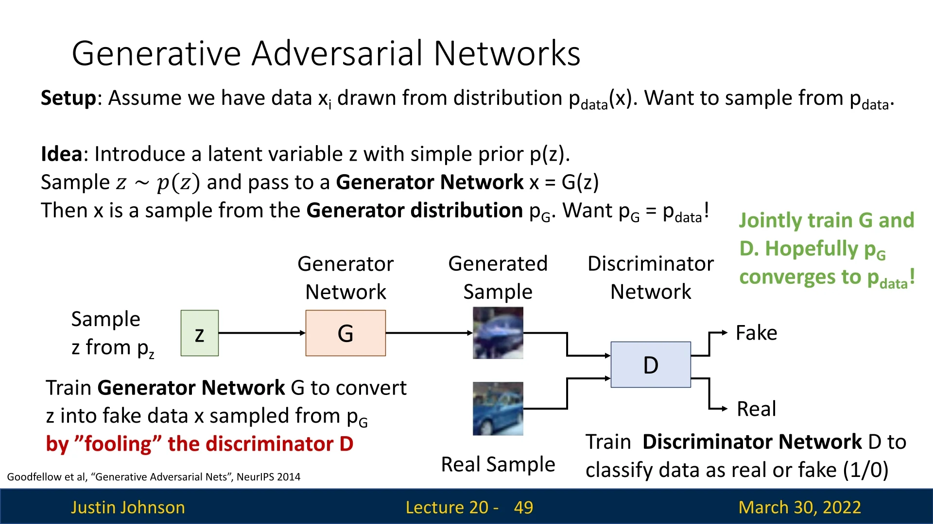
Sampling from the True Distribution Let \( \mathbf {x} \sim p_{\mbox{data}}(\mathbf {x}) \) be a sample from the real data distribution — for instance, natural images. This distribution is unknown and intractable to express, but we assume we have access to i.i.d. samples from it (e.g., a dataset of images).
Our goal is to train a model whose samples are indistinguishable from those of \( p_{\mbox{data}} \). To this end, we adopt a latent variable model:
- Define a simple latent distribution \( p(\mathbf {z}) \), such as a standard Gaussian \( \mathcal {N}(0, \mathbf {I}) \) or uniform distribution.
- Sample a latent code \( \mathbf {z} \sim p(\mathbf {z}) \).
- Pass it through a neural network generator \( \mathbf {x} = G(\mathbf {z}) \) to produce a data sample.
This defines a generator distribution \( p_G(\mathbf {x}) \), where the sampling path is: \[ \mathbf {z} \sim p(\mathbf {z}) \quad \Rightarrow \quad \mathbf {x} = G(\mathbf {z}) \sim p_G(\mathbf {x}) \]
The key challenge is that we cannot write down \( p_G(\mathbf {x}) \) explicitly — it is an implicit distribution defined by the transformation of noise through a neural network.
Discriminator as a Learned Judge To bring \( p_G \) closer to \( p_{\mbox{data}} \), GANs introduce a second neural network: the discriminator \( D(\mathbf {x}) \), which is trained as a binary classifier. It receives samples from either the real distribution \( p_{\mbox{data}} \) or the generator \( p_G \), and must learn to classify them as: \[ D(\mathbf {x}) = \begin {cases} 1 & \mbox{if } \mathbf {x} \sim p_{\mbox{data}} \ (\mbox{real}) \\ 0 & \mbox{if } \mathbf {x} \sim p_G \ (\mbox{fake}) \end {cases} \]
The generator \( G \), meanwhile, is trained to fool the discriminator — it learns to produce samples that the discriminator cannot distinguish from real data.
Adversarial Training Dynamics The result is a two-player game: the generator tries to minimize the discriminator’s ability to detect fakes, while the discriminator tries to maximize its classification accuracy.
- The discriminator \( D \) is trained to maximize the probability of correctly identifying real vs. generated data.
- The generator \( G \) is trained to minimize this probability — i.e., to make generated data look real.
At equilibrium, the discriminator is maximally uncertain (i.e., it assigns probability 0.5 to all inputs), and the generator’s distribution \( p_G \) matches the real distribution \( p_{\mbox{data}} \).
Core Intuition The fundamental idea of GANs is to reframe generative modeling as a discrimination problem: if we can’t explicitly define what makes a good image, we can still train a network to tell real from fake — and then invert this process to generate better samples.
In the next part, we will formalize this game-theoretic setup and introduce the original GAN loss proposed by Goodfellow et al. [186], including its connection to Jensen–Shannon divergence, optimization challenges, and variants.
20.4.2 GAN Training Objective
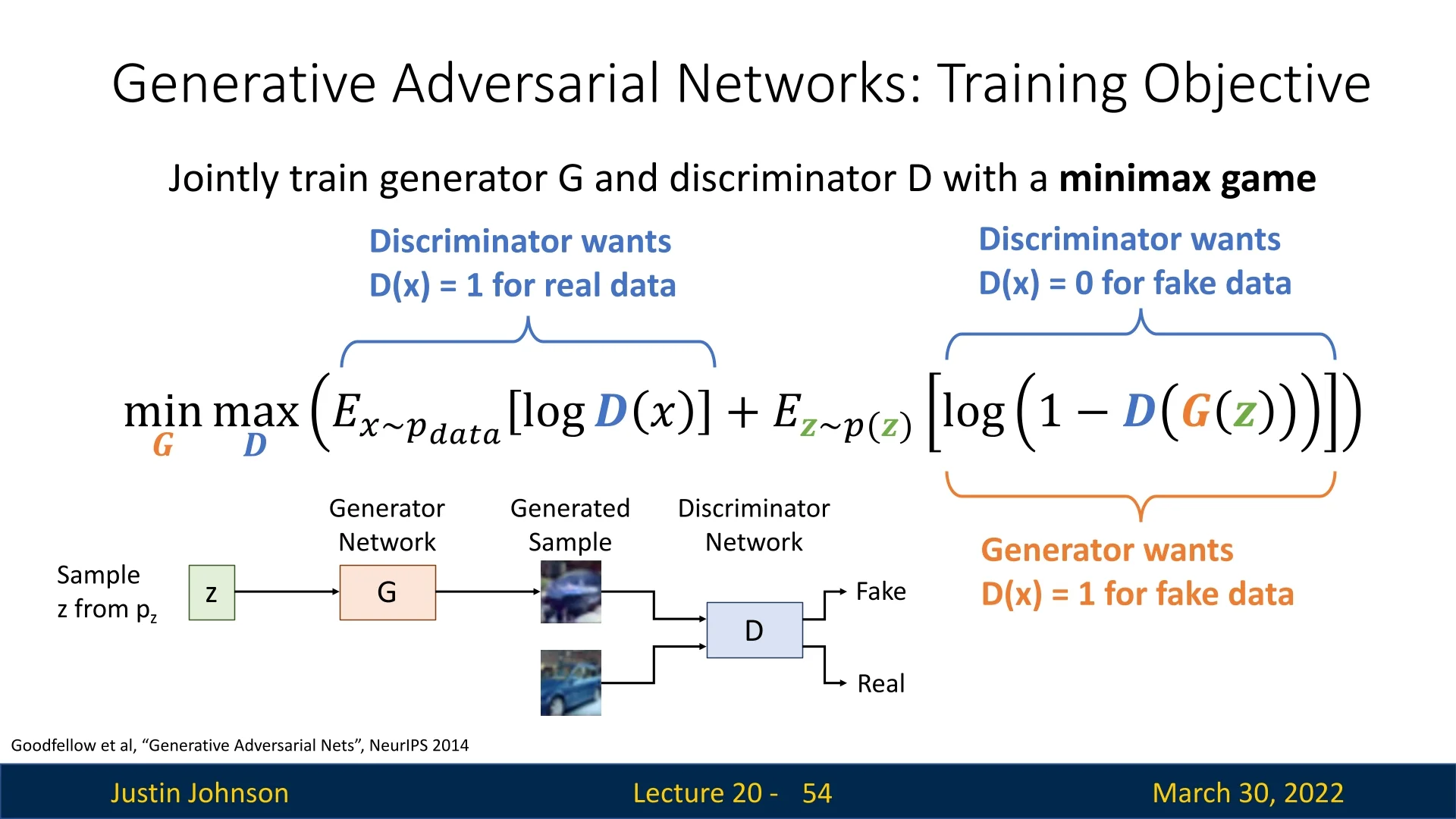
We define a two-player minimax game between \( G \) and \( D \). The discriminator aims to classify real vs. fake images, while the generator tries to fool the discriminator. The objective function is: \[ \min _G \max _D \; V(D, G) = \mathbb {E}_{\mathbf {x} \sim p_{\mbox{data}}} \left [ \log D(\mathbf {x}) \right ] + \mathbb {E}_{\mathbf {z} \sim p(\mathbf {z})} \left [ \log (1 - D(G(\mathbf {z}))) \right ] \]
-
The discriminator maximizes both terms:
- \( \log D(\mathbf {x}) \) encourages \( D \) to classify real data as real (i.e., \( D(\mathbf {x}) \rightarrow 1 \)).
- \( \log (1 - D(G(\mathbf {z}))) \) encourages \( D \) to classify generated samples as fake (i.e., \( D(G(\mathbf {z})) \rightarrow 0 \)).
- The generator minimizes the second term: \[ \mathbb {E}_{\mathbf {z} \sim p(\mathbf {z})} \left [ \log (1 - D(G(\mathbf {z}))) \right ] \] This term is minimized when \( D(G(\mathbf {z})) \rightarrow 1 \), i.e., when the discriminator believes generated samples are real.
The generator and discriminator are trained jointly using alternating gradient updates: \[ \mbox{for } t = 1, \dots , T: \begin {cases} D \leftarrow D + \alpha _D \nabla _D V(G, D) \\ G \leftarrow G - \alpha _G \nabla _G V(G, D) \end {cases} \]
Difficulties in Optimization GAN training is notoriously unstable due to the adversarial dynamics. Two critical issues arise:
- No single loss is minimized: GAN training is a minimax game. The generator and discriminator influence each other’s gradients, making it difficult to assess convergence or use standard training curves.
-
Vanishing gradients early in training: When \( G \) is untrained, it produces unrealistic images. This makes it easy for \( D \) to assign \( D(G(\mathbf {z})) \approx 0 \), saturating the term \( \log (1 - D(G(\mathbf {z}))) \). Since \( \log (1 - x) \) flattens near \( x = 0 \), this leads to vanishing gradients for the generator early on.
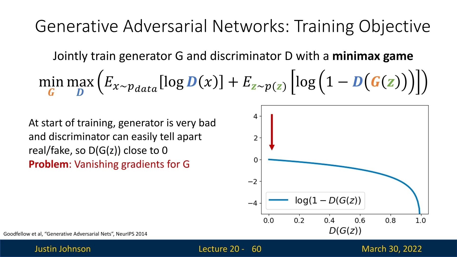
Figure 20.15: At the start of training, the generator produces poor samples. The discriminator easily identifies them, yielding vanishing gradients for the generator.
Modified Generator Loss (Non-Saturating Trick) In the original minimax objective proposed in [186], the generator is trained to minimize: \[ \mathbb {E}_{\mathbf {z} \sim p(\mathbf {z})} \left [ \log (1 - D(G(\mathbf {z}))) \right ] \] This objective encourages \( G \) to generate images that the discriminator believes are real. However, it suffers from a critical problem early in training: when the generator is poor and produces unrealistic images, the discriminator assigns very low scores \( D(G(\mathbf {z})) \approx 0 \). As a result, \( \log (1 - D(G(\mathbf {z}))) \approx 0 \), and its gradient vanishes: \[ \frac {\mathrm {d}}{\mathrm {d}G} \log (1 - D(G(\mathbf {z}))) \rightarrow 0 \]
This leads to extremely weak updates to the generator — just when it needs them most.
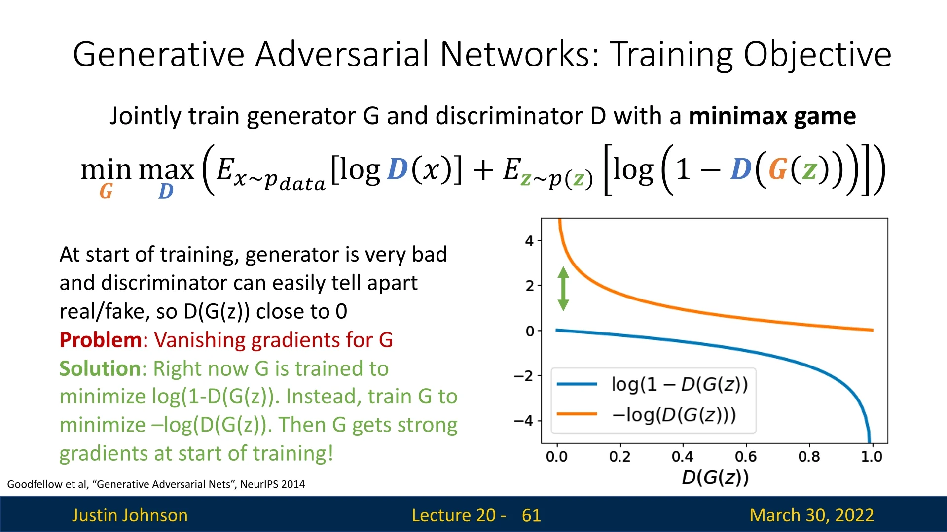
Solution: Switch the Objective Instead of minimizing \( \log (1 - D(G(\mathbf {z}))) \), we train the generator to maximize: \[ \mathbb {E}_{\mathbf {z} \sim p(\mathbf {z})} \left [ \log D(G(\mathbf {z})) \right ] \]
This change does not alter the goal — the generator still wants the discriminator to classify its outputs as real — but it yields stronger gradients, especially when \( D(G(\mathbf {z})) \) is small (i.e., when the discriminator is confident the generated image is fake).
Why does this work?
- For small inputs, \( \log (1 - x) \) is nearly flat (leading to vanishing gradients), while \( \log (x) \) is sharply sloped.
- So when \( D(G(\mathbf {z})) \) is close to zero, minimizing \( \log (1 - D(G(\mathbf {z}))) \) gives negligible gradients, while maximizing \( \log (D(G(\mathbf {z}))) \) gives large, informative gradients.
This variant is known as the non-saturating generator loss, and is widely used in practice for training stability.
Looking Ahead: Why This Objective? We have introduced the practical GAN training objective. But why this specific formulation? Is it theoretically sound? What happens when \( D \) is optimal? Does the generator recover the true data distribution \( p_{\mbox{data}} \)? In the next section, we analyze these questions and uncover the theoretical justification for adversarial training.
20.4.3 Why the GAN Training Objective Is Optimal
Step-by-Step Derivation We begin with the original minimax GAN objective from [186]. Our goal is to analyze the equilibrium of this game by characterizing the global minimum of the value function.
\begin {align*} \min _{\textcolor {darkorange}{G}} \max _{\textcolor {lightblue}{D}} \; & \mathbb {E}_{x \sim p_{\text {data}}}[\log \textcolor {lightblue}{D}(x)] + \mathbb {E}_{\textcolor {lightgreen}{z} \sim p(\textcolor {lightgreen}{z})}[\log (1 - \textcolor {lightblue}{D}(\textcolor {darkorange}{G}(\textcolor {lightgreen}{z})))] \quad \text {(Initial GAN objective)} \\ = \min _{\textcolor {darkorange}{G}} \max _{\textcolor {lightblue}{D}} \; & \mathbb {E}_{x \sim p_{\text {data}}}[\log \textcolor {lightblue}{D}(x)] + \mathbb {E}_{x \sim p_{\textcolor {darkorange}{G}}}[\log (1 - \textcolor {lightblue}{D}(x))] \quad \text {(Change of variables / LOTUS)} \\ = \min _{\textcolor {darkorange}{G}} \max _{\textcolor {lightblue}{D}} \; & \int _{\mathcal {X}} \left ( p_{\text {data}}(x) \log \textcolor {lightblue}{D}(x) + p_{\textcolor {darkorange}{G}}(x) \log (1 - \textcolor {lightblue}{D}(x)) \right ) dx \quad \text {(Definition of expectation)} \\ = \min _{\textcolor {darkorange}{G}} \; & \int _{\mathcal {X}} \max _{\textcolor {lightblue}{D(x)}} \left ( p_{\text {data}}(x) \log \textcolor {lightblue}{D}(x) + p_{\textcolor {darkorange}{G}}(x) \log (1 - \textcolor {lightblue}{D}(x)) \right ) dx \quad \text {(Push $\max _{\textcolor {lightblue}{D}}$ inside integral)} \end {align*}
Justification of the Mathematical Transformations To rigorously justify the steps above, we appeal to measure theory and the calculus of variations.
-
Change of Variables (The Pushforward and LOTUS):
The second term in the original objective is expressed as an expectation over latent variables \( \textcolor {lightgreen}{z} \sim p(\textcolor {lightgreen}{z}) \), with samples transformed through the generator: \( x = \textcolor {darkorange}{G}(\textcolor {lightgreen}{z}) \). This defines a new distribution over images, denoted \( \textcolor {darkorange}{p_G}(x) \), formally known as the pushforward measure (or generator distribution).The transition from an expectation over \( \textcolor {lightgreen}{z} \) to one over \( x \) is a direct application of the Law of the Unconscious Statistician (LOTUS). It guarantees that: \[ \mathbb {E}_{\textcolor {lightgreen}{z} \sim p(\textcolor {lightgreen}{z})} \left [ \log \left (1 - \textcolor {lightblue}{D}(\textcolor {darkorange}{G}(\textcolor {lightgreen}{z})) \right ) \right ] \quad \Rightarrow \quad \mathbb {E}_{x \sim \textcolor {darkorange}{p_G}(x)} \left [ \log \left (1 - \textcolor {lightblue}{D}(x) \right ) \right ] \] This reparameterization is valid because the pushforward distribution \( p_G \) exists. For the integral notation used subsequently, we further assume \( p_G \) admits a density with respect to the Lebesgue measure.
- Expectation to Integral:
Any expectation over a continuous random variable can be written as an integral: \[ \mathbb {E}_{x \sim p(x)}[f(x)] = \int _{\mathcal {X}} p(x) f(x) \, dx \] This applies to both the real data term and the generator term, allowing us to combine them into a single integral over the domain \( \mathcal {X} \). -
Pushing \( \max _D \) into the Integral (Functional Separability):
The discriminator \( \textcolor {lightblue}{D} \) is treated here as an arbitrary function defined pointwise over the domain \( \mathcal {X} \). This is an assumption of non-parametric optimization (i.e., we assume \( D \) has infinite capacity and is not constrained by a neural network architecture).Crucially, there is no dependence or coupling between \( \textcolor {lightblue}{D}(x_1) \) and \( \textcolor {lightblue}{D}(x_2) \) for different values of \( x \). Therefore, the objective functional is separable, and maximizing the global integral is equivalent to maximizing the integrand independently for each \( x \). \[ \max _{\textcolor {lightblue}{D}} \int _{\mathcal {X}} \cdots \; dx \quad \Longrightarrow \quad \int _{\mathcal {X}} \max _{\textcolor {lightblue}{D}(x)} \cdots \; dx \]
Solving the Inner Maximization (Discriminator) We now optimize the integrand pointwise for each \( x \in \mathcal {X} \), treating the discriminator output \( \textcolor {purple}{y} = \textcolor {purple}{D(x)} \) as a scalar variable. Define the objective at each point as: \[ f(\textcolor {purple}{y}) = \textcolor {darkred}{a} \log \textcolor {purple}{y} + \textcolor {darkeryellow}{b} \log (1 - \textcolor {purple}{y}), \quad \mbox{with} \quad \textcolor {darkred}{a} = p_{\mbox{data}}(x), \; \textcolor {darkeryellow}{b} = p_G(x) \] This function is strictly concave on \( \textcolor {purple}{y} \in (0, 1) \), and we compute the maximum by solving \( f'(\textcolor {purple}{y}) = 0 \): \[ f'(\textcolor {purple}{y}) = \frac {\textcolor {darkred}{a}}{\textcolor {purple}{y}} - \frac {\textcolor {darkeryellow}{b}}{1 - \textcolor {purple}{y}} = 0 \quad \Rightarrow \quad \textcolor {purple}{y} = \frac {\textcolor {darkred}{a}}{\textcolor {darkred}{a} + \textcolor {darkeryellow}{b}} \] Substituting back, the optimal value for the discriminator is: \[ \textcolor {lightblue}{D}^{*}_{\textcolor {darkorange}{G}}(x) = \frac {\textcolor {darkred}{p_{\mbox{data}}(x)}}{\textcolor {darkred}{p_{\mbox{data}}(x)} + \textcolor {darkeryellow}{p_G(x)}} \]
Here’s how the components map:
- \( p_{\mbox{data}}(x) \) (red) is the true data distribution at \( x \).
- \( D(x) \) (purple) is the scalar output of the discriminator.
- \( p_G(x) \) (dark yellow) is the generator’s distribution at \( x \).
This solution gives us the discriminator’s best possible output for any fixed generator \( G \). In the next step, we will plug this optimal discriminator back into the GAN objective to simplify the expression and reveal its connection to divergence measures.
Plugging the Optimal Discriminator into the Objective Having found the optimal discriminator \( \textcolor {lightblue}{D}^*_{\textcolor {darkorange}{G}} \) for a fixed generator, we now substitute it back into the game to evaluate the generator’s performance.
Recall that our goal is to minimize the value function \( V(\textcolor {darkorange}{G}, \textcolor {lightblue}{D}) \). Since the inner maximization is now solved, we focus on the Generator Value Function \( C(\textcolor {darkorange}{G}) \), which represents the generator’s loss when facing a perfect adversary: \[ C(\textcolor {darkorange}{G}) = \max _{\textcolor {lightblue}{D}} V(\textcolor {darkorange}{G}, \textcolor {lightblue}{D}) = V(\textcolor {darkorange}{G}, \textcolor {lightblue}{D}^*_{\textcolor {darkorange}{G}}) \]
To perform the substitution, let us first simplify the terms involving the optimal discriminator. Given \( \textcolor {lightblue}{D}^*_{\textcolor {darkorange}{G}}(x) = \frac {\textcolor {darkred}{p_{\mbox{data}}(x)}}{\textcolor {darkred}{p_{\mbox{data}}(x)} + \textcolor {darkeryellow}{p_G(x)}} \), the complementary probability (probability that the discriminator thinks a fake sample is fake) is: \[ 1 - \textcolor {lightblue}{D}^*_{\textcolor {darkorange}{G}}(x) = 1 - \frac {\textcolor {darkred}{p_{\mbox{data}}(x)}}{\textcolor {darkred}{p_{\mbox{data}}(x)} + \textcolor {darkeryellow}{p_G(x)}} = \frac {\textcolor {darkeryellow}{p_G(x)}}{\textcolor {darkred}{p_{\mbox{data}}(x)} + \textcolor {darkeryellow}{p_G(x)}} \]
We now replace \( \textcolor {lightblue}{D}(x) \) and \( (1-\textcolor {lightblue}{D}(x)) \) in the original integral objective with these expressions: \begin {align*} \min _{\textcolor {darkorange}{G}} C(\textcolor {darkorange}{G}) & = \min _{\textcolor {darkorange}{G}} \int _{\mathcal {X}} \Bigg ( \underbrace {\textcolor {darkred}{p_{\text {data}}(x)} \log \left ( \frac {\textcolor {darkred}{p_{\text {data}}(x)}} {\textcolor {darkred}{p_{\text {data}}(x)} + \textcolor {darkeryellow}{p_G(x)}} \right )}_{\text {Expected log-prob of real data}} + \underbrace {\textcolor {darkeryellow}{p_G(x)} \log \left ( \frac {\textcolor {darkeryellow}{p_G(x)}} {\textcolor {darkred}{p_{\text {data}}(x)} + \textcolor {darkeryellow}{p_G(x)}} \right )}_{\text {Expected log-prob of generated data}} \Bigg ) dx \end {align*}
Rewriting as KL Divergences The expression above resembles Kullback–Leibler (KL) divergence, but the denominators are sums, not distributions. To fix this, we need to compare \( \textcolor {darkred}{p_{\mbox{data}}} \) and \( \textcolor {darkeryellow}{p_G} \) against their average distribution (or mixture): \[ m(x) = \frac {\textcolor {darkred}{p_{\mbox{data}}(x)} + \textcolor {darkeryellow}{p_G(x)}}{2} \] We manipulate the log arguments by multiplying numerator and denominator by \( 2 \). This ”trick” is mathematically neutral (multiplying by \( 1 \)) but structurally revealing:
\begin {align*} = \min _{\textcolor {darkorange}{G}} \Bigg ( & \int _{\mathcal {X}} \textcolor {darkred}{p_{\text {data}}(x)} \log \left ( \frac {1}{2} \cdot \frac {\textcolor {darkred}{p_{\text {data}}(x)}}{\frac {\textcolor {darkred}{p_{\text {data}}(x)} + \textcolor {darkeryellow}{p_G(x)}}{2}} \right ) dx \\ + & \int _{\mathcal {X}} \textcolor {darkeryellow}{p_G(x)} \log \left ( \frac {1}{2} \cdot \frac {\textcolor {darkeryellow}{p_G(x)}}{\frac {\textcolor {darkred}{p_{\text {data}}(x)} + \textcolor {darkeryellow}{p_G(x)}}{2}} \right ) dx \Bigg ) \end {align*}
Using the logarithmic identity \( \log (a \cdot b) = \log a + \log b \), we separate the fraction \( \frac {1}{2} \) from the ratio of distributions. Note that \( \log (1/2) = -\log 2 \):
\begin {align*} = \min _{\textcolor {darkorange}{G}} \Bigg ( & \int _{\mathcal {X}} \textcolor {darkred}{p_{\text {data}}(x)} \left [ \log \left ( \frac {\textcolor {darkred}{p_{\text {data}}(x)}}{m(x)} \right ) - \log 2 \right ] dx \\ + & \int _{\mathcal {X}} \textcolor {darkeryellow}{p_G(x)} \left [ \log \left ( \frac {\textcolor {darkeryellow}{p_G(x)}}{m(x)} \right ) - \log 2 \right ] dx \Bigg ) \end {align*}
We now distribute the integrals. Since \( \textcolor {darkred}{p_{\mbox{data}}} \) and \( \textcolor {darkeryellow}{p_G} \) are valid probability distributions, they integrate to 1. Therefore, the constant terms \( -\log 2 \) sum to \( -2\log 2 = -\log 4 \). The remaining integrals are, by definition, KL divergences:
\begin {align*} = \min _{\textcolor {darkorange}{G}} \Bigg ( KL\left ( \textcolor {darkred}{p_{\text {data}}} \Big \| \frac {\textcolor {darkred}{p_{\text {data}}} + \textcolor {darkeryellow}{p_G}}{2} \right ) + KL\left ( \textcolor {darkeryellow}{p_G} \Big \| \frac {\textcolor {darkred}{p_{\text {data}}} + \textcolor {darkeryellow}{p_G}}{2} \right ) - \log 4 \Bigg ) \end {align*}
Introducing the Jensen–Shannon Divergence (JSD) The expression inside the minimization is related to the Jensen–Shannon Divergence (JSD), which measures the similarity between two probability distributions. Unlike KL divergence, JSD is symmetric and bounded. It is defined as: \[ JSD(p, q) = \frac {1}{2} KL\left ( p \Big \| \frac {p + q}{2} \right ) + \frac {1}{2} KL\left ( q \Big \| \frac {p + q}{2} \right ) \]
Final Result: Objective Minimizes JSD Substituting the JSD definition into our derived expression, the GAN training objective reduces to: \begin {align*} \min _{\textcolor {darkorange}{G}} C(\textcolor {darkorange}{G}) = \min _{\textcolor {darkorange}{G}} \left ( 2 \cdot JSD\left ( \textcolor {darkred}{p_{\text {data}}}, \textcolor {darkeryellow}{p_G} \right ) - {\log 4} \right ) \end {align*}
Interpretation:
- 1.
- The term \( -\log 4 \) represents the value of the game when the generator is perfect (confusion). Since \( \log 4 = 2 \log 2 \), this corresponds to the discriminator outputting \( 0.5 \) (uncertainty) for both real and fake samples: \( \log (0.5) + \log (0.5) = -\log 4 \).
- 2.
- Since \( JSD(p, q) \geq 0 \) with equality if and only if \( p = q \), the global minimum is achieved exactly when: \[ \textcolor {darkeryellow}{p_G(x)} = \textcolor {darkred}{p_{\mbox{data}}(x)} \]
This completes the proof: under idealized conditions (infinite capacity discriminator), the minimax game forces the generator to perfectly recover the data distribution.
Summary \begin {align*} \text {Optimal discriminator:} \quad &\textcolor {lightblue}{D}^{*}_{\textcolor {darkorange}{G}}(x) = \frac {\textcolor {darkred}{p_{\text {data}}(x)}}{\textcolor {darkred}{p_{\text {data}}(x)} + \textcolor {darkeryellow}{p_G(x)}} \\ \text {Global minimum:} \quad &\textcolor {purple}{p_G(x)} = \textcolor {darkred}{p_{\text {data}}(x)} \end {align*}
Important Caveats and Limitations of the Theoretical Result The optimality result derived above provides a crucial theoretical anchor: it guarantees that the minimax objective is statistically meaningful, identifying the data distribution as the unique global optimum. However, bridging the gap between this idealized theory and practical deep learning requires navigating several critical limitations.
-
Idealized Functional Optimization vs. Parameterized Networks. The derivation treats the discriminator \( D \) (and implicitly the generator \( G \)) as ranging over the space of all measurable functions. This ”non-parametric” or ”infinite capacity” assumption is what allows us to solve the inner maximization problem \(\max _D V(G,D)\) pointwise for every \( x \), yielding the closed-form \( D_G^* \).
In practice, we optimize over restricted families of functions parameterized by neural network weights, \( D_\phi \) and \( G_\theta \). The shared weights in a network introduce coupling between outputs—changing parameters to update \( D(x_1) \) inevitably affects \( D(x_2) \). Consequently: (i) The network family may not be expressive enough to represent the sharp, pointwise optimal discriminator \( D_G^* \); and (ii) Even if representable, the non-convex optimization landscape of the parameters may prevent gradient descent from finding it. Thus, the theorem proves that the game has the correct solution, not that a specific architecture trained with SGD will necessarily reach it.
-
The “Manifold Problem” and Vanishing Gradients. The JSD interpretation relies on the assumption that \( p_{\mbox{data}} \) and \( p_G \) have overlapping support with well-defined densities. In high-dimensional image spaces, however, distributions often concentrate on low-dimensional manifolds (e.g., the set of valid face images is a tiny fraction of the space of all possible pixel combinations).
Early in training, these real and generated manifolds are likely to be disjoint. In this regime, a sufficiently capable discriminator can separate the distributions perfectly, setting \( D(x) \approx 1 \) on real data and \( D(x) \approx 0 \) on fake data. Mathematically, this causes the Jensen–Shannon divergence to saturate at its maximum value (constant \(\log 2\)). Since the gradient of a constant is zero, the generator receives no informative learning signal to guide it toward the data manifold. This geometry is the primary cause of the vanishing gradient problem in the original GAN formulation and motivates alternative objectives (like the non-saturating heuristic or Wasserstein distance) designed to provide smooth gradients even when distributions do not overlap.
-
Existence vs. Convergence (Statics vs. Dynamics). The proof characterizes the static equilibrium of the game: if we reach a state where \( p_G = p_{\mbox{data}} \), we are at the global optimum. It says nothing about the dynamics of reaching that state.
GAN training involves finding a saddle point of a non-convex, non-concave objective using alternating stochastic gradient updates. Such dynamical systems are prone to pathologies that simple minimization avoids, including: (i) Limit cycles, where the generator and discriminator chase each other in circles (rotational dynamics) without improving; (ii) Divergence, where gradients grow uncontrollably; and (iii) Mode collapse, where the generator maps all latent codes to a single ”safe” output that fools the discriminator, satisfying the local objective but failing to capture the full diversity of the data distribution.
20.5 GANs in Practice: From Early Milestones to Modern Advances
20.5.1 The Original GAN (2014)
In their seminal work [186], Goodfellow et al. demonstrated that GANs could be trained to synthesize digits similar to MNIST and low-resolution human faces. While primitive by today’s standards, this was a significant leap: generating samples that look realistic without explicitly modeling likelihoods.
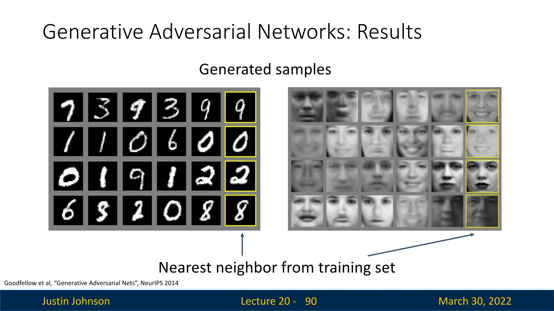
20.5.2 Deep Convolutional GAN (DCGAN)
The Deep Convolutional GAN (DCGAN) architecture, proposed by Radford et al. [510], marked a significant step toward stabilizing GAN training and improving the visual quality of generated images. Unlike the original fully connected GAN setup, DCGAN leverages the power of convolutional neural networks to better model image structure and achieve more coherent generations.
Architectural Innovations and Design Principles
- Convolutions instead of Fully Connected Layers: DCGAN eliminates dense layers at the input and output of the networks. Instead, it starts from a low-dimensional latent vector \( \mathbf {z} \sim \mathcal {N}(0, I) \) and progressively upsamples it through a series of transposed convolutions (also called fractional-strided convolutions) in the generator. This preserves spatial locality and improves feature learning.
- Strided Convolutions (Downsampling): The discriminator performs downsampling using strided convolutions rather than max pooling. This approach allows the network to learn its own spatial downsampling strategy rather than rely on a hand-designed pooling operation, thereby improving gradient flow and learning stability.
-
Fractional-Strided Convolutions (Upsampling): In the generator, latent codes are transformed into images through a series of transposed convolutions. These layers increase the spatial resolution of the feature maps while learning spatial structure, enabling the model to produce high-resolution outputs from compact codes.
- Batch Normalization: Applied in both the generator and discriminator (except the generator’s output layer and discriminator’s input layer), batch normalization smooths the learning dynamics and helps mitigate issues like mode collapse. It also reduces internal covariate shift, allowing higher learning rates and more stable convergence.
- Activation Functions: The generator uses ReLU activations in all layers except the output, which uses tanh to map values into the \([-1, 1]\) range. The discriminator uses LeakyReLU activations throughout, which avoids dying neuron problems and provides gradients even for negative inputs.
- No Pooling or Fully Connected Layers: The absence of pooling layers and fully connected components ensures the entire network remains fully convolutional, further reinforcing locality and translation equivariance.
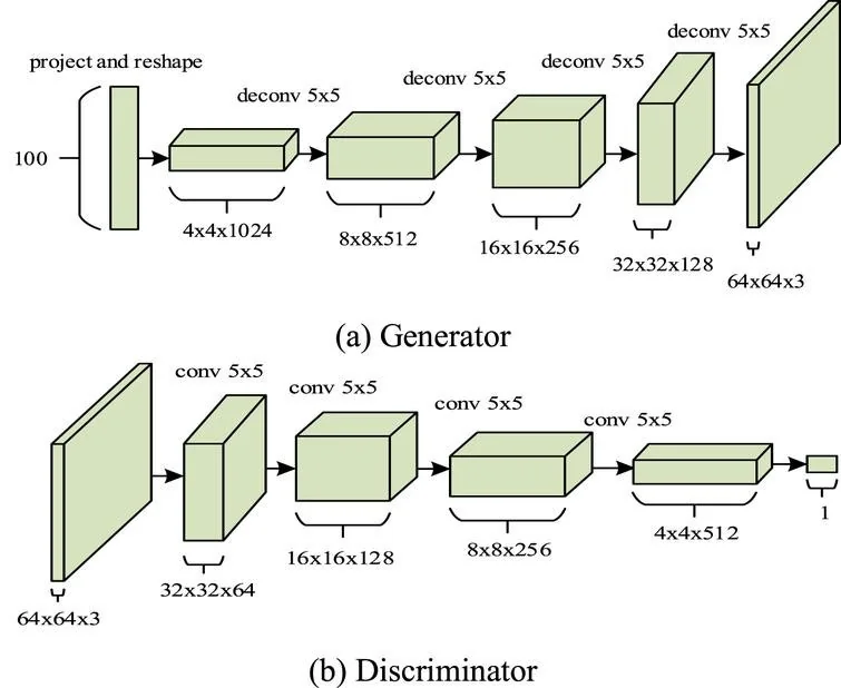
Why it Works These design choices reflect the successful architectural heuristics of supervised CNNs (e.g., AlexNet, VGG) but adapted to the generative setting. The convolutional hierarchy builds up spatially coherent features, while batch normalization and careful activation design help maintain gradient signal throughout training. As a result, DCGANs are capable of producing high-quality samples on natural image datasets with far greater stability than the original GAN formulation.
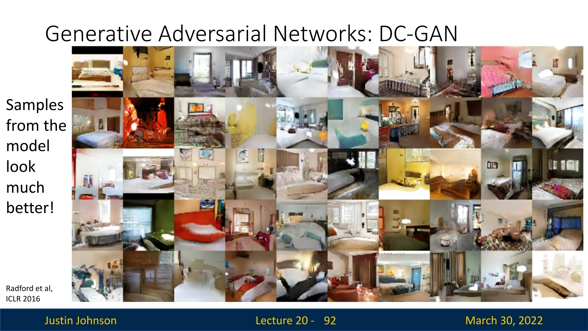
Latent Space Interpolation One striking property of DCGAN is that interpolating between two latent codes \( \mathbf {z}_1 \) and \( \mathbf {z}_2 \) leads to smooth transitions in image space: \[ G((1-\alpha )\mathbf {z}_1 + \alpha \mathbf {z}_2), \quad \alpha \in [0, 1] \]
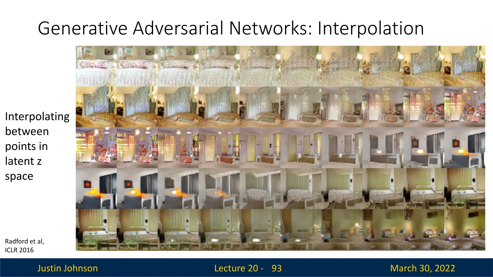
Latent Vector Arithmetic
DCGAN also revealed that semantic attributes can be disentangled in the latent space \( \mathbf {z} \). Consider the following operation:
\[ \mbox{smiling man} \approx \underbrace { \mbox{mean}(\mathbf {z}_{\mbox{smiling women}}) }_{\mbox{attribute: smile}} - \underbrace { \mbox{mean}(\mathbf {z}_{\mbox{neutral women}}) }_{\mbox{remove woman identity}} + \underbrace { \mbox{mean}(\mathbf {z}_{\mbox{neutral men}}) }_{\mbox{add male identity}} \]
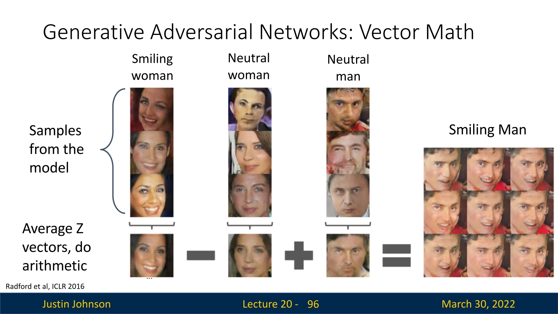
A similar example uses glasses as a visual attribute: \[ \mathbf {z}_{\mbox{woman with glasses}} = \mathbf {z}_{\mbox{man with glasses}} - \mathbf {z}_{\mbox{man without glasses}} + \mathbf {z}_{\mbox{woman without glasses}} \]
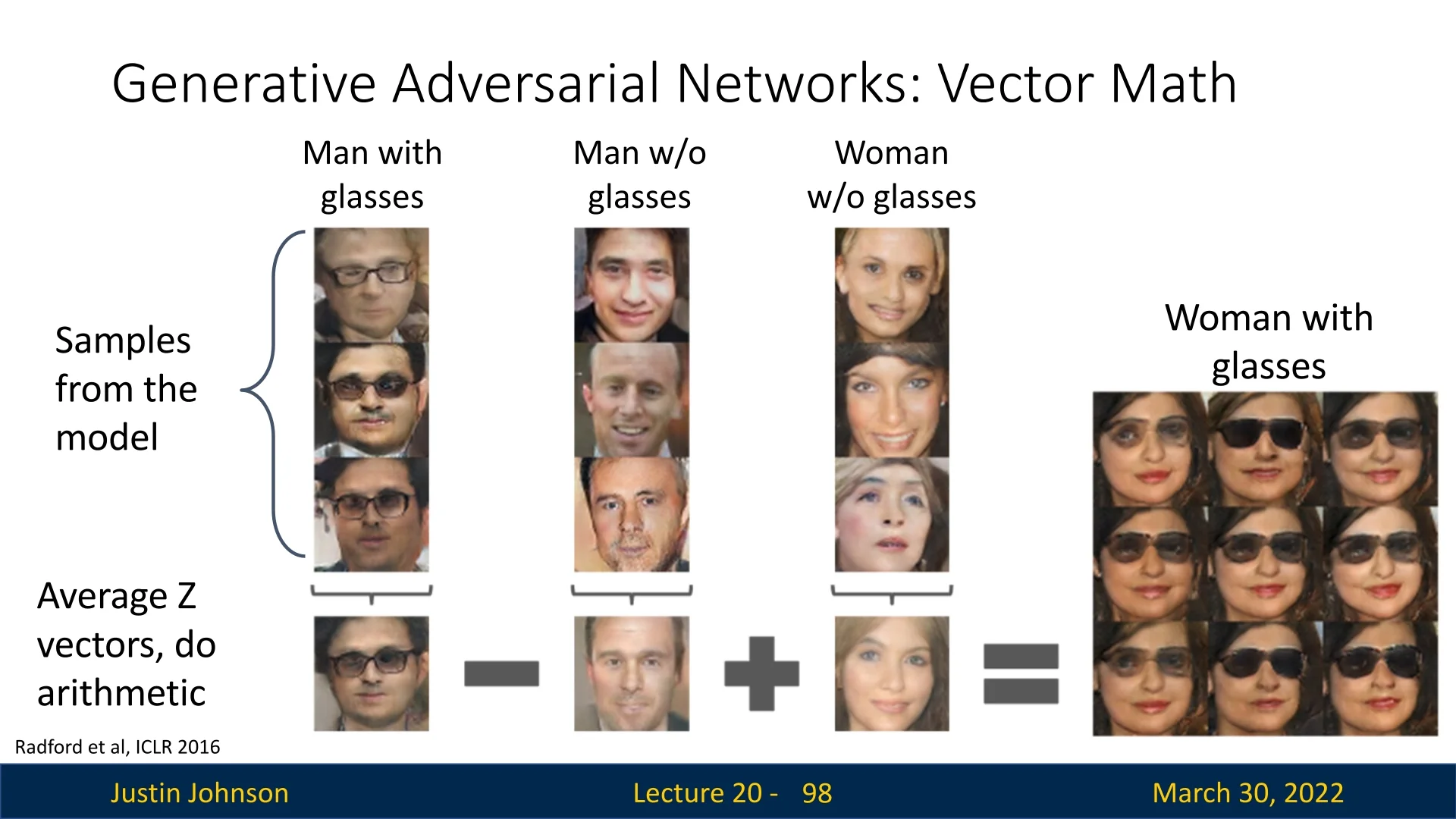
Evaluating Generative Adversarial Networks (GANs)
Evaluating generative adversarial networks (GANs) remains one of the most important (and still imperfectly solved) problems in generative modeling. Unlike likelihood-based models (e.g., VAEs), standard GAN training does not yield a tractable scalar objective such as \(\log p_\theta (x)\) that can be directly used for model selection. Instead, as derived in the previous section, GANs optimize a minimax objective whose theoretical global optimum forces the generator to perfectly recover the data distribution (\(p_G = p_{\mbox{data}}\)), thereby minimizing the Jensen-Shannon Divergence (JSD).
Ideally, reaching this global minimum would satisfy all evaluation needs simultaneously. In practice, however, we must evaluate the generator’s partial success along three distinct axes, each rooted in the min-max formulation:
- 1.
- Fidelity (Realism): Do individual samples look real?
Min-Max mechanism: Enforced by the discriminator \(D\). To minimize JSD, the generator must ensure \(p_G(x)\) is non-zero only where \(p_{\mbox{data}}(x)\) is high. If \(G\) generates samples outside the manifold of real data, the optimal discriminator \(D^*\) easily identifies and penalizes them. - 2.
- Diversity / Coverage: Does the model represent all modes of the
data?
Min-Max mechanism: Theoretically mandated by the condition \(p_G = p_{\mbox{data}}\). The JSD is only zero if \(G\) covers every mode of the target distribution with the correct density. (In practice, however, optimization instability often leads to mode collapse, where \(G\) captures only a single mode to satisfy \(D\)). - 3.
- Semantic Correctness: (Optional) Does the model respect
conditioning?
Min-Max mechanism: In conditional GANs, the adversarial game extends to joint distributions. The discriminator forces \(p_G(x,y)\) to match \(p_{\mbox{data}}(x,y)\), ensuring that generated samples \(x\) are not just realistic, but correctly aligned with their labels \(y\).
Since the training loss value (ideally \(-\log 4\)) is often uninformative about which of these properties is being satisfied or violated, modern practice relies on a bundle of external checks and scores [560, 412].
A practical rule: metrics are only comparable under the same protocol Absolute scores (especially FID/KID) are generally not portable across different datasets, resolutions, feature extractors, or preprocessing pipelines. Therefore, whenever you report a quantitative score, you should also report the evaluation protocol: the real split used (train vs. held-out test), image resolution, number of generated samples, the feature extractor \(\phi (\cdot )\), and the exact preprocessing (in particular, resizing and cropping policy). In practice, protocol differences can easily cause score swings that are comparable to (or larger than) architectural gains.
Qualitative vs. quantitative evaluation We divide evaluation methods into two main categories: qualitative (human judgment, nearest-neighbor checks) and quantitative (feature-space distribution metrics such as IS, FID, KID, and precision/recall).
Qualitative Evaluation Methods
Manual inspection and preference ranking The simplest evaluation technique is visual inspection of samples. Human judges may rate realism, compare images side-by-side, or choose which model produces higher-quality samples.
In practice, this is often implemented via crowd-sourcing (e.g., Amazon Mechanical Turk) or via blinded pairwise preference tests [560]. The advantage is sensitivity to “semantic failures” that scalar metrics may miss (odd textures, broken geometry, repeated artifacts). The drawbacks are that it is subjective, expensive, and difficult to scale to large sweeps or to reproduce exactly.
Nearest-neighbor retrieval (memorization / leakage sanity check) A standard diagnostic is to test whether generated samples are near-duplicates of training examples. Given a generated image \(x_g\), retrieve its nearest neighbor among a reference set of real images \(\{x_r\}\) using a perceptual similarity measure.
Important: Pixel-space \(\ell _2\) is typically misleading (tiny translations can dominate \(\ell _2\) while being visually negligible), so in practice one uses deep features (e.g., Inception/DINO/CLIP embeddings) or perceptual distances such as LPIPS [800]. Qualitatively inspecting pairs \((x_g,\mathrm {NN}(x_g))\) can reveal direct copying. However, note the asymmetry of this test: “not identical to a training image” is not a proof of generalization; it is only a guardrail against the most obvious memorization failure modes.
Quantitative Evaluation Methods
Most modern metrics compare distributions of embeddings Many widely used GAN metrics begin by embedding images with a fixed, pretrained feature extractor \(\phi (\cdot )\in \mathbb {R}^d\) (classically Inception-v3 pool3 features). One then compares the empirical distributions of real embeddings \(\{\phi (x_r)\}\) and generated embeddings \(\{\phi (x_g)\}\). This is both a strength and a limitation: the metric becomes sensitive to the semantics captured by \(\phi \), and insensitive to aspects \(\phi \) ignores. This dependence is especially important under domain shift (e.g., medical images), where ImageNet-pretrained features may be a weak proxy for perceptual similarity.
Inception Score (IS) Proposed by [560], the Inception Score uses a pretrained classifier \(p_\phi (y\mid x)\) to reward two properties: (i) confidence on each generated sample (low conditional entropy \(H(Y\mid X)\)), and (ii) label diversity across samples (high marginal entropy \(H(Y)\)). Let \(p_\phi (y)=\mathbb {E}_{x\sim p_G}[p_\phi (y\mid x)]\). Then \[ \mathrm {IS} \;=\; \exp \!\left ( \mathbb {E}_{x\sim p_G}\!\left [ D_{\mathrm {KL}}\!\big (p_\phi (y\mid x)\,\|\,p_\phi (y)\big ) \right ]\right ). \] While IS historically appears in many papers, it is often de-emphasized in modern reporting because it has several structural limitations:
- No real-vs.-fake comparison: IS depends only on generated samples, so it can increase even if samples drift away from the true data distribution.
- Classifier and label-set bias: its meaning depends on whether the pretrained classifier is appropriate for the domain.
- Can miss intra-class mode collapse: generating one “prototype” per class can yield a strong IS while having poor within-class diversity.
Fréchet Inception Distance (FID) The Fréchet Inception Distance (FID) [227] improves upon IS by directly comparing real and generated feature distributions. Given real images \(\{x_r\}\) and generated images \(\{x_g\}\), compute embeddings \(u=\phi (x_r)\) and \(v=\phi (x_g)\), estimate empirical means and covariances \((\mu _r,\Sigma _r)\) and \((\mu _g,\Sigma _g)\), and define the squared 2-Wasserstein (Fréchet) distance between the corresponding Gaussians: \[ \mathrm {FID} \;=\; \|\mu _r-\mu _g\|_2^2 \;+\; \mathrm {Tr}\!\Big ( \Sigma _r+\Sigma _g - 2\big (\Sigma _r^{1/2}\,\Sigma _g\,\Sigma _r^{1/2}\big )^{1/2} \Big ). \]
Intuitively, the mean term \(\|\mu _r-\mu _g\|_2^2\) captures a shift/bias between the feature clouds, while the covariance term captures mismatch in spread and correlations (often aligned with diversity and mode coverage). This real-vs.-fake distribution comparison is the main reason FID became a de facto standard.
How to interpret FID (and why “typical ranges” are only rough)
- Lower is better: smaller FID indicates closer alignment between real and generated feature distributions under \(\phi \).
- Non-zero even for real-vs.-real: if you compute FID between two finite real sample sets, it is typically non-zero due to sampling noise.
- Context-dependent scale: absolute values depend strongly on dataset, resolution, and protocol; the safest use of FID is relative comparison under a fixed evaluation pipeline.
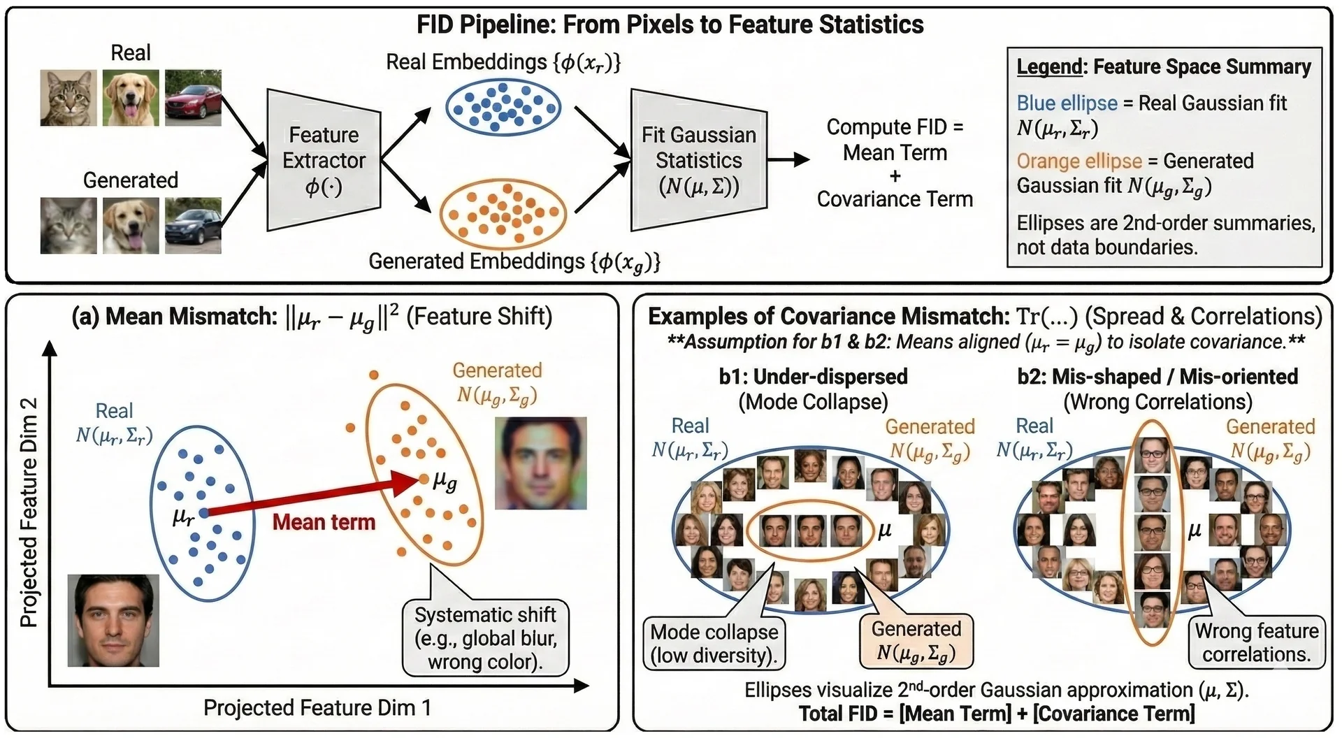
FID limitations and implementation pitfalls (often the main source of confusion)
- Second-order (Gaussian) summary: FID matches only first and second moments of \(\phi (x)\); real feature distributions are typically multi-modal, so \((\mu ,\Sigma )\) is a coarse approximation.
- Preprocessing sensitivity: resizing interpolation, cropping, and normalization can measurably change FID. For fair comparisons, treat preprocessing as part of the metric definition (“CleanFID-style” discipline: fixed, explicit preprocessing and extractor).
- Finite-sample effects: FID is a biased estimator with nontrivial variance at small sample sizes; comparisons are most meaningful when computed with a large, fixed sample budget and (ideally) repeated across random seeds/splits.
- Domain mismatch (feature-extractor bias): Inception features encode ImageNet semantics. For domains far from ImageNet, it is common to replace \(\phi \) with a domain-relevant encoder (supervised or self-supervised), but then scores become extractor-specific and must not be compared across different choices of \(\phi \).
A Note on Reconstruction Metrics (PSNR, SSIM, LPIPS) Readers coming from classical image restoration (denoising, deblurring, super-resolution) often report PSNR or SSIM. These are paired (reference-based) metrics: they require a pixel-aligned ground-truth target \(x\) and a prediction \(\hat {x}\). This makes them appropriate for supervised tasks (where a single “correct” answer exists) but fundamentally mismatched to unconditional GAN synthesis (where no unique target exists) and often misleading even for conditional GANs.
-
Peak Signal-to-Noise Ratio (PSNR). PSNR is simply a logarithmic rescaling of the pixelwise Mean Squared Error (MSE): \[ \mathrm {PSNR}(x,\hat {x}) = 10\log _{10}\!\left (\frac {\mathrm {MAX}_I^2}{\mathrm {MSE}(x,\hat {x})}\right ), \] where \(\mathrm {MAX}_I\) is the maximum dynamic range (e.g., 255).
Why it fails for GANs: MSE relies on pixel-wise \(\ell _2\) distance. It treats a tiny spatial shift (e.g., a nose moved by 1 pixel) as a massive error, yet it rewards blurring (averaging) because the mean of many plausible edges minimizes the squared error. GANs, designed to produce sharp, hallucinated details, often have poor PSNR despite superior perceptual quality.
-
Structural Similarity Index (SSIM). SSIM attempts to quantify perceptual similarity by comparing local statistics of image patches rather than raw pixels. For two patches \(x\) and \(\hat {x}\), SSIM is the product of three terms: \[ \mathrm {SSIM}(x,\hat {x}) = \underbrace {l(x,\hat {x})^\alpha }_{\mbox{Luminance}} \cdot \underbrace {c(x,\hat {x})^\beta }_{\mbox{Contrast}} \cdot \underbrace {s(x,\hat {x})^\gamma }_{\mbox{Structure}} \] 1. Why do these terms match human perception? SSIM maps statistical moments to visual concepts:
- Luminance (Mean \(\mu \)): The average pixel intensity \(\mu _x\) corresponds directly to the patch’s brightness. A global lighting shift affects \(\mu \) but leaves the content intact.
- Contrast (Variance \(\sigma \)): The standard deviation \(\sigma _x\) measures the signal amplitude. A flat grey patch has \(\sigma =0\) (no contrast), while a sharp edge has high \(\sigma \). Blurring acts as a low-pass filter, reducing \(\sigma \), which SSIM penalizes as a loss of contrast.
- Structure (Covariance \(\sigma _{x\hat {x}}\)): The normalized correlation measures if the patterns align (e.g., do gradients point in the same direction?) regardless of their absolute brightness or amplitude.
2. Why SSIM fails for Semantic Realism: While better than PSNR, SSIM is still a low-level statistic. It checks if local edges align, not if the image makes sense. A generated face with distorted anatomy (e.g., an eye on the chin) might have excellent local contrast and texture statistics (high SSIM if aligned to a reference), while being semantically broken. Conversely, a plausible dog generated in a slightly different pose than the reference will suffer a huge penalty.
LPIPS: Perceptual Similarity in Deep Feature Space To bridge the gap between pixel metrics and human perception, LPIPS (Learned Perceptual Image Patch Similarity) [800] measures distance in the activation space of a pre-trained deep network (e.g., VGG or AlexNet). \[ \mathrm {LPIPS}(x,\hat {x}) = \sum _{\ell } \| w_\ell \odot (\psi _\ell (x) - \psi _\ell (\hat {x})) \|_2^2 \] Unlike PSNR, which sees a ”bag of pixels”, LPIPS sees ”hierarchy of features”. It correctly identifies that a sharp, texture-rich image is closer to reality than a blurry average, even if the pixels don’t align perfectly.
Other Quantitative Metrics (Complements, Not Replacements) Since unconditional GANs cannot use paired metrics, we rely on distributional metrics to diagnose specific failure modes.
-
Precision and Recall (Manifold Approximation) [558]. These metrics separate Fidelity (Precision) from Coverage (Recall).
How are they measured without the true manifold? Since we cannot know the true high-dimensional manifold, we approximate it using \(k\)-Nearest Neighbors (\(k\)-NN) balls around the available data samples in feature space.
- Precision (Quality): What % of generated samples fall within the \(k\)-NN balls of the real data? (If low: generating garbage).
- Recall (Diversity): What % of real samples fall within the \(k\)-NN balls of the generated data? (If low: mode collapse).
-
Kernel Inception Distance (KID) [45]. KID is a non-parametric alternative to FID. Instead of assuming feature embeddings follow a Gaussian distribution, KID measures the squared Maximum Mean Discrepancy (MMD) between the real and generated distributions in a reproducing kernel Hilbert space (RKHS).
1. Feature Embeddings (\(X\) and \(Y\)). Like FID, KID operates in the feature space of a pre-trained network \(\phi (\cdot )\) (usually Inception-v3). We define two sets of embeddings: \[ X = \{\phi (x_r^{(i)})\}_{i=1}^m \quad (\mbox{Real}), \qquad Y = \{\phi (x_g^{(j)})\}_{j=1}^n \quad (\mbox{Generated}). \] Note that the sample sizes \(m\) and \(n\) need not be equal. This is practically useful when the test set size is fixed (e.g., \(m=10,000\)) but you wish to evaluate a smaller batch of generated samples (\(n=2,000\)) for efficiency.
2. The Metric: Unbiased MMD. KID compares these sets using a polynomial kernel function, typically \(k(u,v) = (\frac {1}{d}u^\top v + 1)^3\). The metric is computed via an unbiased estimator composed of three terms: \[ \widehat {\mathrm {KID}} = \underbrace {\frac {1}{m(m-1)}\sum _{i\neq i'} k(x_i, x_{i'})}_{\mbox{Average Real--Real Similarity}} \;+\; \underbrace {\frac {1}{n(n-1)}\sum _{j\neq j'} k(y_j, y_{j'})}_{\mbox{Average Gen--Gen Similarity}} \;-\; \underbrace {\frac {2}{mn}\sum _{i=1}^m \sum _{j=1}^n k(x_i, y_j)}_{\mbox{Average Real--Gen Similarity}} \]
3. Intuition and Advantages. Conceptually, the formula measures ”cohesion vs. separation”: if the distributions match, the average cross-similarity (real vs. generated) should equal the average self-similarity (real vs. real).
- Unbiasedness: The primary advantage of KID over FID is that its estimator is unbiased. FID systematically overestimates the distance when \(N\) is small (bias \(\propto 1/N\)). KID’s expected value equals the true population distance regardless of sample size.
- Practical Use: This makes KID the standard choice for small datasets, few-shot generation, or limited compute budgets where generating 50,000 samples for stable FID is infeasible.
-
Classifier Two-Sample Tests (C2ST). This involves training a new, separate binary classifier to distinguish Real vs. Fake samples after the GAN is trained.
- If Accuracy \(\approx \) 50%: The distributions are indistinguishable (Perfect GAN).
- If Accuracy \(\gg \) 50%: The classifier can spot the fakes.
Difference from GAN Discriminator: The GAN discriminator is part of the dynamic training game (moving target). C2ST is a static ”post-game referee” that provides a sanity check on whether the final result is truly indistinguishable.
- Geometry Score (GS) [302]. While FID measures density, GS measures Topology (shape complexity). It builds a graph of the data manifold and compares topological features like ”number of holes” or ”connected components”. Intuition: If the real data forms a single connected ring (like a donut) but the GAN generates two disconnected blobs, FID might be low (blobs are in the right place), but GS will penalize the broken connectivity (wrong topology).
Optional but important when editing matters: Latent-Space Diagnostics Metrics like FID evaluate the destination (the final distribution of images). They do not tell us about the journey—specifically, whether the latent space is well-structured for editing and interpolation. For models like StyleGAN, we use Perceptual Path Length (PPL) [289] to quantify the ”smoothness” of the latent manifold.
The Intuition: Smooth vs. Rugged Landscapes. Imagine walking in a straight line through the latent space. In a disentangled (good) space, a small step results in a small, consistent visual change (e.g., a face slowly turning). In an entangled (bad) space, the same small step might cause sudden, erratic jumps (e.g., a face suddenly changing identity or artifacts appearing and disappearing). PPL measures this ”bumpiness”.
How is it computed?
- 1.
- Interpolate: Pick two latent codes \(z_1, z_2\) and take a tiny step \(\epsilon \) along the path between them (usually using spherical interpolation, slerp).
- 2.
- Generate: Decode the images at the start and end of this tiny step: \(x = G(z(t))\) and \(x' = G(z(t+\epsilon ))\).
- 3.
- Measure: Calculate the perceptual distance \(d = \mbox{LPIPS}(x, x')\).
- 4.
- Normalize: PPL is the expected value of this distance normalized by the step size \(\epsilon ^2\).
Interpretation:
- Low PPL (Good): The latent space is perceptually uniform. Changes in latent values map linearly to changes in visual appearance, making the model reliable for animation and editing.
- High PPL (Bad): The latent space contains ”hidden” non-linearities or singularities where the image changes drastically (or breaks) over short distances.
Limitations and Practical Guidelines
Robust evaluation requires Protocol Discipline. Absolute scores are meaningless without context.
- Report the Protocol: Always specify resolution, feature extractor (e.g., Inception-v3), and resizing method (CleanFID).
- Triangulate: Never rely on one number. Pair a distributional metric (FID/KID) with a diagnostic metric (Precision/Recall).
- Qualitative Guardrails: Always visually inspect nearest neighbors. A perfect FID of 0.0 means nothing if the model simply memorized the training set.
Summary Evaluating GANs is difficult precisely because there is no single, universally meaningful scalar objective. In practice, the most reliable approach is protocol discipline plus metric triangulation: report a real-vs.-fake distribution metric (FID or KID), decompose fidelity vs. coverage (precision–recall), and keep qualitative sanity checks (inspection and nearest neighbors). When Inception features are a poor fit for the domain, the feature extractor must be treated as part of the metric definition, and comparisons should be restricted accordingly.
20.5.3 GAN Explosion
These results sparked rapid growth in the GAN research landscape, with hundreds of new papers and variants proposed every year. For a curated (and still growing) collection of GAN papers, see: The GAN Zoo.
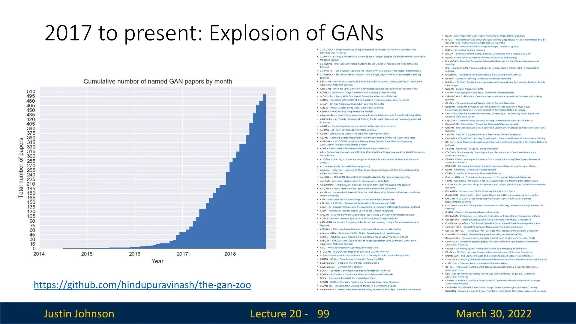
Next Steps: Improving GANs While the original GAN formulation [186] introduced a powerful framework, it often suffers from instability, vanishing gradients, and mode collapse during training. These issues led to a wave of improvements that we now explore in the following sections. Notable directions include:
- Wasserstein GAN (WGAN) — replaces the Jensen–Shannon-based loss with the Earth Mover’s (Wasserstein) distance for smoother gradients.
- WGAN-GP — introduces a gradient penalty to enforce Lipschitz constraints without weight clipping.
- StyleGAN / StyleGAN2 — enables high-resolution image synthesis with disentangled and controllable latent spaces.
- Conditional GANs (cGANs) — allows conditioning the generation process on labels, text, or other modalities.
These innovations make GANs more robust, interpretable, and scalable — paving the way for practical applications in vision, art, and science.
20.5.4 Wasserstein GAN (WGAN): Earth Mover’s Distance
While original GANs achieved impressive qualitative results, their training can be highly unstable and sensitive to hyperparameters. A key theoretical issue is that, under an optimal discriminator, the original minimax GAN objective reduces to a constant plus a Jensen–Shannon (JS) divergence term between \(p_{\mbox{data}}\) and \(p_G\) [186]. In high-dimensional settings where the two distributions often lie on (nearly) disjoint low-dimensional manifolds, this JS-based perspective helps explain why the learning signal can become weak or poorly behaved. Below, we revisit this failure mode and then introduce Wasserstein GAN (WGAN) [14], which replaces JS with the Wasserstein-1 (Earth Mover) distance to obtain a smoother, geometry-aware objective.
Supports and Low-Dimensional Manifolds
- Support of a distribution: The subset of space where the distribution assigns non-zero probability. In high-dimensional data like images, real samples lie on or near a complex, low-dimensional manifold (e.g., the “face manifold” of all possible human faces).
- Generator manifold: Similarly, the generator’s outputs \(G(z)\) with \(z \sim p(z)\) occupy their own manifold. Initially, the generator manifold often lies far from the data manifold.
Why the JS Divergence Fails in High Dimensions In the original minimax GAN game, if the discriminator is optimized for a fixed generator, the value function can be written as a constant plus a Jensen–Shannon divergence term [186]: \[ \max _D \; V(G,D) = -\log 4 + 2\,JS\!\left (p_{\mbox{data}} \,\|\, p_G\right ). \] Thus, improving the generator in the idealized setting corresponds to reducing a JS-based discrepancy between \(p_{\mbox{data}}\) and \(p_G\). However, when these distributions have disjoint support, this discrepancy saturates and yields a poorly behaved learning signal:
- Early training (negligible overlap): The generator typically produces unrealistic outputs, so \(p_G\) has little overlap with \(p_{\mbox{data}}\). Ideally, we want a gradient that points towards the data. However, the JS divergence saturates to a constant (\(\log 2\)) when supports are disjoint, providing no smooth notion of “distance” to guide the generator.
- Weak or unreliable generator signal near an optimal discriminator: As the discriminator becomes very accurate, its outputs saturate (\(D(x)\approx 1\) on real, \(D(G(z))\approx 0\) on fake). This can yield vanishing or highly localized gradients for the generator, making training brittle and contributing to mode collapse.
Non-Saturating Trick: A Partial Fix. To mitigate immediate vanishing gradients, Goodfellow et al. [186] proposed replacing the minimax generator objective with a different (but still consistent) surrogate.
In the original formulation, the generator minimizes the probability of the discriminator being correct: \begin {equation} \mathcal {L}_G^{\mbox{minimax}} = \mathbb {E}_{z \sim p(z)}[\log (1 - D(G(z)))]. \end {equation} When the discriminator is strong (common early in training), \(D(G(z)) \approx 0\). In this region, the function \(\log (1 - x)\) saturates—it becomes flat, yielding near-zero gradients.
The non-saturating alternative instead maximizes the discriminator’s output on fake samples: \begin {equation} \max _G\;\mathbb {E}_{z \sim p(z)}[\log D(G(z))] \quad \Longleftrightarrow \quad \min _G\;\mathcal {L}_G^{\mbox{NS}} = -\mathbb {E}_{z \sim p(z)}[\log D(G(z))]. \end {equation} Why it helps: Although the optimum point theoretically remains the same, the gradient dynamics differ. The function \(-\log (x)\) rises sharply as \(x \to 0\). This ensures the generator receives a strong gradient signal precisely when it is performing poorly (i.e., when \(D(G(z)) \approx 0\)), kickstarting the learning process.
The Need for a Better Distance Metric Ultimately, the issue is not with the choice of generator loss formulation alone — it’s with the divergence measure itself. Wasserstein GANs (WGANs) address this by replacing JS with the Wasserstein-1 distance, also known as the Earth Mover’s Distance (EMD). Unlike JS, the Wasserstein distance increases smoothly as the distributions move apart and remains informative even when they are fully disjoint. It directly measures how much and how far the probability mass needs to be moved to align \( p_G \) with \( p_{\mbox{data}} \). As a result, WGANs produce gradients that are:
- Typically less prone to saturation than JS-based objectives when the critic is trained near its optimum.
- More reflective of distributional geometry (how mass must move), rather than only separability.
- Better aligned with incremental improvements in sample quality, often yielding smoother and more stable optimization in practice.
This theoretical improvement forms the basis of WGANs, laying the foundation for more stable and expressive generative training — even before considering architectural or loss refinements like gradient penalties in WGAN-GP [201], which we’ll cover later as well.
Wasserstein-1 Distance: Transporting Mass The Wasserstein-1 distance — also called the Earth Mover’s Distance (EMD) — quantifies how much “mass” must be moved to transform the generator distribution \( p_G \) into the real data distribution \( p_{\mbox{data}} \), and how far that mass must travel. Formally: \[ W(p_{\mbox{data}}, p_G) = \inf _{\gamma \in \Pi (p_{\mbox{data}}, p_G)} \, \mathbb {E}_{(x, y) \sim \gamma } \left [ \|x - y\| \right ] \]
Here:
- \( \gamma (x, y) \) is a transport plan, i.e., a joint distribution describing how much mass to move from location \( y \sim p_G \) to location \( x \sim p_{\mbox{data}} \).
- The set \(\Pi (p_{\mbox{data}}, p_G)\) contains all valid couplings—that is, joint distributions \(\gamma (x, y)\) whose marginals match the source and target distributions. Concretely, \(\gamma \) must satisfy: \begin {equation} \int \gamma (x, y) \, dy = p_{\mbox{data}}(x) \quad \mbox{and} \quad \int \gamma (x, y) \, dx = p_G(y). \end {equation} (In discrete settings, these integrals become sums). This constraint ensures mass conservation: no probability mass is created or destroyed; it is simply moved from \(y\) to \(x\).
- The infimum (\( \inf \)) takes the best (lowest cost) over all possible plans \( \gamma \in \Pi \).
- The cost function \( \|x - y\| \) reflects how far one must move a unit of mass from \( y \) to \( x \). It is often Euclidean distance, but other choices are possible.
Example: Optimal Transport Plans as Joint Tables To see this in action, consider a simple example in 1D:
- Generator distribution \( p_G \): 0.5 mass at \( y_1 = 0 \), and 0.5 at \( y_2 = 4 \).
- Data distribution \( p_{\mbox{data}} \): 0.5 mass at \( x_1 = 2 \), and 0.5 at \( x_2 = 3 \).
Each plan defines a joint distribution \( \gamma (x, y) \) specifying how much mass to move between source and target locations.
Plan 1 (Optimal): \[ \gamma _{\mbox{plan 1}}(x, y) = \begin {array}{c|cc} & y=0 & y=4 \\ \hline x=2 & 0.5 & 0.0 \\ x=3 & 0.0 & 0.5 \\ \end {array} \quad \Rightarrow \quad \mbox{Cost} = 0.5\cdot |2{-}0| + 0.5\cdot |3{-}4| = 1 + 0.5 = \boxed {1.5} \]
Plan 2 (Suboptimal): \[ \gamma _{\mbox{plan 2}}(x, y) = \begin {array}{c|cc} & y=0 & y=4 \\ \hline x=2 & 0.0 & 0.5 \\ x=3 & 0.5 & 0.0 \\ \end {array} \quad \Rightarrow \quad \mbox{Cost} = 0.5\cdot |3{-}0| + 0.5\cdot |2{-}4| = 1.5 + 1 = \boxed {2.5} \]
Plan 3 (Mixed): \[ \gamma _{\mbox{plan 3}}(x, y) = \begin {array}{c|cc} & y=0 & y=4 \\ \hline x=2 & 0.25 & 0.25 \\ x=3 & 0.25 & 0.25 \\ \end {array} \quad \Rightarrow \quad \mbox{Cost} = \sum \gamma (x, y)\cdot |x{-}y| = \boxed {2.0} \]
Each table represents a valid joint distribution \( \gamma \in \Pi (p_{\mbox{data}}, p_G) \), since the row and column sums match the marginal probabilities. The Wasserstein-1 distance corresponds to the cost of the optimal plan, i.e., the one with lowest total transport cost.
- Meaningful even with disjoint support: Unlike JS (which saturates at \(\log 2\) under disjoint support in the idealized analysis), Wasserstein-1 continues to vary with the geometric separation between distributions.
- Captures geometric mismatch: It does not merely say “different”; it encodes how far probability mass must move under an optimal coupling.
- Potentially informative signal early in training: When the critic is trained near its optimum and the Lipschitz constraint is controlled, the resulting gradients can remain useful even when \(p_G\) is far from the data manifold.
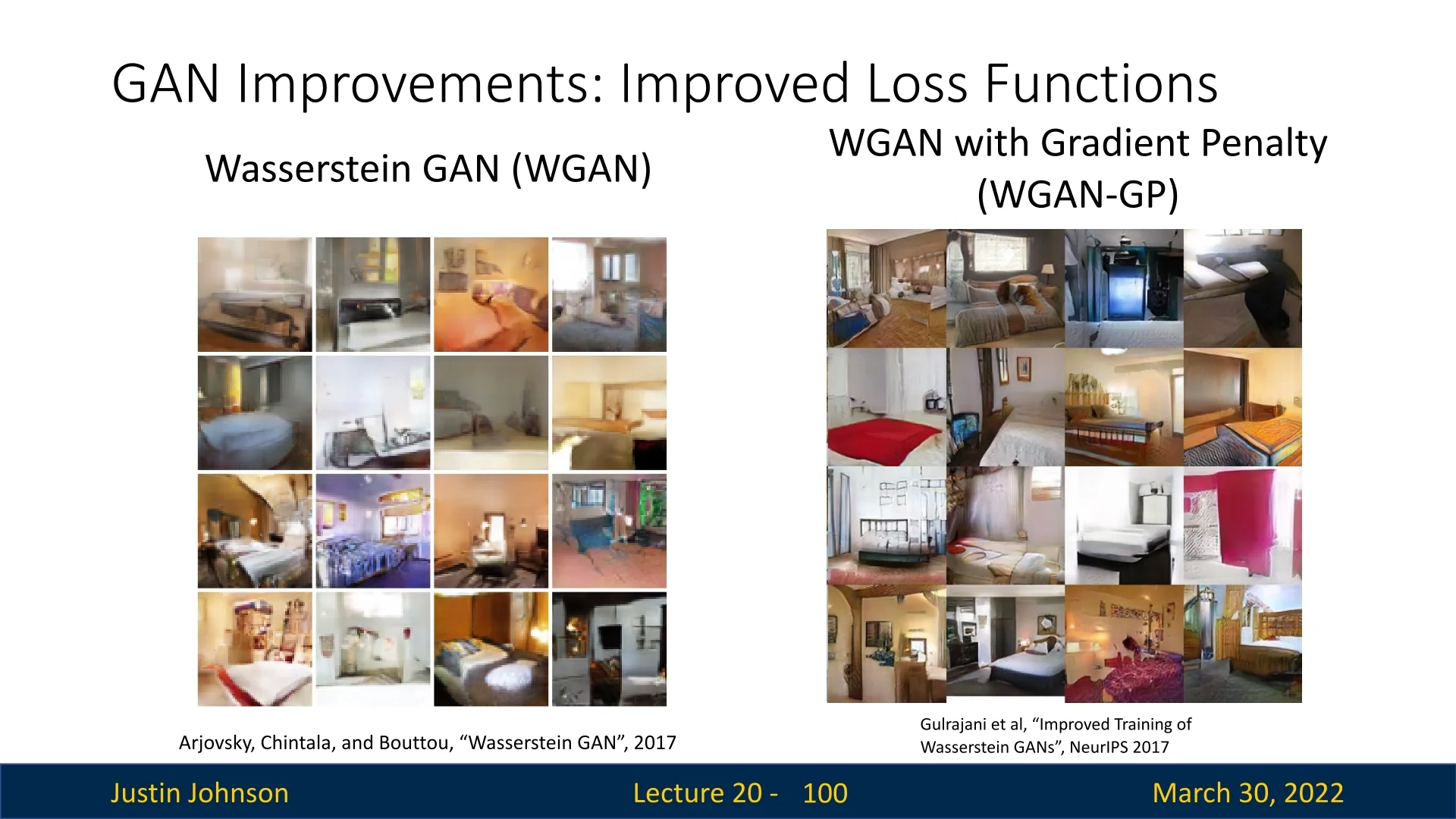
From Intractable Transport to Practical Training The Wasserstein-1 distance offers a theoretically sound objective that avoids the saturation problems of JS divergence. However, its original definition involves a highly intractable optimization over all possible joint couplings: \[ W(p_{\mbox{data}}, p_G) = \inf _{\gamma \in \Pi (p_{\mbox{data}}, p_G)} \, \mathbb {E}_{(x, y) \sim \gamma } \left [ \|x - y\| \right ] \] Computing this infimum directly is not feasible for high-dimensional distributions like images.
The Kantorovich–Rubinstein duality makes the problem tractable by recasting it as: \[ W(p_{\mbox{data}}, p_G) = \sup _{\|f\|_L \leq 1} \left ( \mathbb {E}_{x \sim p_{\mbox{data}}} [f(x)] - \mathbb {E}_{\tilde {x} \sim p_G} [f(\tilde {x})] \right ), \] where the supremum is taken over all 1-Lipschitz functions \( f \colon \mathcal {X} \to \mathbb {R} \).
What These Expectations Mean in Practice In actual training, we do not have access to the full distributions \( p_{\mbox{data}} \) and \( p_G \), but only to samples. The expectations are therefore approximated by empirical means over minibatches: \[ \mathbb {E}_{x \sim p_{\mbox{data}}}[f(x)] \;\approx \; \frac {1}{m} \sum _{i=1}^{m} f(x^{(i)}), \qquad \mathbb {E}_{\tilde {x} \sim p_G}[f(\tilde {x})] \;\approx \; \frac {1}{m} \sum _{i=1}^{m} f(G(z^{(i)})), \] where:
- \( \{x^{(i)}\}_{i=1}^m \) is a minibatch sampled from the training dataset \( p_{\mbox{data}} \).
- \( \{z^{(i)}\}_{i=1}^m \sim p(z) \), typically \( \mathcal {N}(0, I) \), is a batch of latent codes.
- \( \tilde {x}^{(i)} = G(z^{(i)}) \) are the generated images.
How the Training Works (Maximize vs. Minimize). In WGAN, the critic \(f_w\) (parameterized by weights \(w\)) is trained to approximate the dual optimum by widening the score gap between real and fake data.
- 1.
- The Critic Loss (Implementation View): Since deep learning frameworks typically minimize loss functions, we invert the dual objective. We minimize the difference: \begin {equation} \mathcal {L}_{\mbox{critic}} = \underbrace {\mathbb {E}_{z \sim p(z)}[f_w(G(z))]}_{\mbox{Score on Fake}} - \underbrace {\mathbb {E}_{x \sim p_{\mbox{data}}}[f_w(x)]}_{\mbox{Score on Real}}. \end {equation} Minimizing this quantity is equivalent to maximizing the score on real data while minimizing it on fake data.
- 2.
- The Generator Loss: The generator is updated to minimize the critic’s score on its output (effectively trying to move its samples “uphill” along the critic’s value surface): \begin {equation} \mathcal {L}_{\mbox{gen}} = -\mathbb {E}_{z \sim p(z)}[f_w(G(z))]. \end {equation}
Intuitively, the critic learns a scalar potential function whose slopes point towards the data manifold, and the generator moves its probability mass to follow these gradients.
Why This Makes Sense — Even if Samples Differ Sharply This training might appear unintuitive at first glance:
- We are not directly comparing real and fake images pixel-by-pixel.
- The generator might produce very different images (e.g., noise) from real data in early training.
Yet, the setup works because:
- The critic learns a scalar-valued function \( f(x) \) that assigns a meaningful score to each image, indicating how realistic it appears under the current critic.
- Even if two distributions have no overlapping support, the critic can still produce distinct outputs for each — preserving a non-zero mean score gap.
- The generator then improves by reducing this gap, pushing \( p_G \) closer to \( p_{\mbox{data}} \) in a distributional sense.
In other words, we do not require individual generated samples to match real ones — only that, on average, the generator learns to produce samples that fool the critic into scoring them similarly.
Summary WGAN training works by:
- 1.
- Using minibatch means to estimate expectations in the dual Wasserstein objective.
- 2.
- Leveraging the critic as a 1-Lipschitz scoring function trained to separate real from fake.
- 3.
- Providing stable, non-vanishing gradients even when real and generated distributions are far apart.
This principled approach turns adversarial training into a smooth, geometry-aware optimization process — and lays the foundation for further improvements like WGAN-GP.
Side-by-Side: Standard GAN vs. WGAN
| Component | Standard GAN | Wasserstein GAN (WGAN) |
|---|---|---|
| Objective | \( \begin {array}{l} \min _G \max _D \bigl [ \mathbb {E}_{x \sim p_{\mbox{data}}} \log D(x) \\ +\, \mathbb {E}_{z \sim p(z)} \log (1 - D(G(z))) \bigr ] \end {array} \) | \( \begin {array}{l} \min _G \max _{\|f\|_L \leq 1} \bigl [ \mathbb {E}_{x \sim p_{\mbox{data}}} f(x) \\ -\, \mathbb {E}_{z \sim p(z)} f(G(z)) \bigr ] \end {array} \) |
| Output Type | \( D(x) \in [0,1] \) (probability) | \( f(x) \in \mathbb {R} \) (score) |
| Interpretation | Probability \( x \) is real | Realism score for \( x \) |
| Training Signal | Jensen–Shannon divergence | Wasserstein-1 (Earth Mover) distance |
| Disjoint Supports | JS saturates to \( \log 2 \); gradients vanish | Distance remains informative (with Lipschitz critic) |
What’s Missing: Enforcing the 1-Lipschitz Constraint The dual WGAN formulation transforms the intractable Wasserstein distance into a solvable optimization problem: \[ W(p_{\mbox{data}}, p_G) = \sup _{\|f\|_L \leq 1} \left ( \mathbb {E}_{x \sim p_{\mbox{data}}}[f(x)] - \mathbb {E}_{x \sim p_G}[f(x)] \right ) \] However, this relies on a crucial condition: the function \( f \) must be 1-Lipschitz — that is, it cannot change too quickly: \[ |f(x_1) - f(x_2)| \leq \|x_1 - x_2\| \quad \forall x_1, x_2 \]
This constraint ensures that the critic’s output is smooth and bounded — a key requirement to preserve the validity of the dual formulation. Yet enforcing this constraint precisely over a deep neural network is non-trivial. To address this, Arjovsky et al. [14] introduce a simple approximation: weight clipping.
Weight Clipping: A Crude Approximation After each gradient update during training, every parameter \( w \) in the critic is constrained to lie within a compact range: \[ w \leftarrow \mbox{clip}(w, -c, +c) \quad \mbox{with} \quad c \approx 0.01 \]
The rationale is that limiting the range of weights constrains the magnitude of the output changes, thereby approximating a 1-Lipschitz function. If the weights are small, then the critic function \( f(x) \) cannot change too rapidly with respect to changes in \( x \).
Benefits of WGAN Despite using a crude approximation like weight clipping to enforce the 1-Lipschitz constraint, Wasserstein GANs (WGAN) demonstrate compelling improvements over standard GANs:
- More interpretable training signal (often): When the critic is trained near its optimum, the WGAN critic loss frequently correlates better with generator progress than standard GAN discriminator losses, making it a more practical monitoring metric.
- Smoother optimization in challenging regimes: Because Wasserstein-1 varies continuously with distributional shifts (including disjoint support), WGAN can yield less saturated and more stable gradients than JS-based objectives, especially early in training.
- Reduced risk of mode collapse (not eliminated): By encouraging the generator to reduce a transport-based discrepancy rather than only improving separability, WGAN training can make collapse less likely in practice, though it does not guarantee full mode coverage.
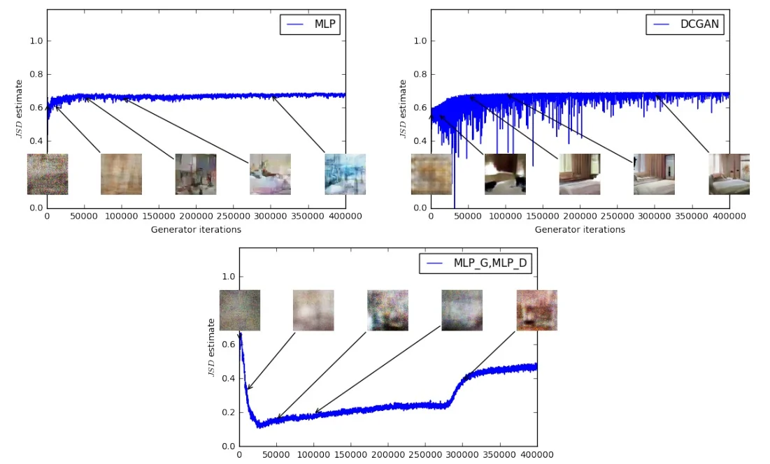
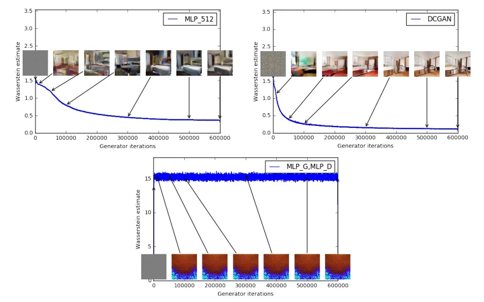
Limitations of Weight Clipping in Practice While simple to implement, weight clipping is an imprecise and inefficient method for enforcing the 1-Lipschitz constraint. It introduces multiple issues that degrade both the expressiveness of the critic and the overall training dynamics:
- Reduced expressivity: Weight clipping constrains each parameter of the critic network to lie within a small range (e.g., \( [-0.01, 0.01] \)). This effectively flattens the critic’s function space, especially in deeper architectures. The resulting networks tend to behave like near-linear functions, as layers with small weights compound to produce low-variance outputs. Consequently, the critic struggles to capture meaningful variations between real and generated data — particularly in complex image domains — leading to weak or non-informative gradients for the generator.
-
Fragile gradient propagation: Gradient-based learning relies on consistent signal flow through layers. When weights are clipped, two opposing issues can arise:
- If weights are too small, the gradients shrink with each layer — leading to vanishing gradients, especially in deep networks.
- If weights remain non-zero but unevenly distributed across layers, activations can spike, causing exploding gradients in certain directions due to unbalanced Jacobians.
These effects are particularly problematic in ReLU-like networks, where clipping reduces activation diversity and gradient feedback becomes increasingly unreliable.
- Training instability and non-smooth loss: Empirical studies (e.g., Figure 4 in [14]) show that critics trained under clipping oscillate unpredictably. In some iterations, the critic becomes too flat to distinguish between real and fake inputs; in others, it becomes overly reactive to minor differences. This leads to high-variance Wasserstein estimates and erratic training curves. Worse, when the critic is underfit, the generator may receive biased or misleading gradients, preventing effective mode coverage or long-term convergence.
Despite these challenges, weight clipping served its purpose in the original WGAN: it provided a proof of concept that optimizing the Wasserstein-1 distance offers substantial advantages over traditional GAN losses. However, it quickly became apparent that a more robust and mathematically faithful mechanism was needed. This inspired Gulrajani et al. [201] to propose WGAN-GP — which enforces Lipschitz continuity via a smooth and principled gradient penalty, significantly improving stability and sample quality.
20.5.5 WGAN-GP: Gradient Penalty for Stable Lipschitz Enforcement
While WGAN introduced a major improvement by replacing the JS divergence with the Wasserstein-1 distance, its dual formulation relies on a key mathematical requirement: the critic \( f \colon \mathcal {X} \to \mathbb {R} \) must be 1-Lipschitz. In the original WGAN, this was enforced via weight clipping, which constrains parameters to a small interval. As discussed, clipping is a coarse proxy for Lipschitz control and often leads to underfitting (an overly simple critic) or brittle optimization.
To address this, Gulrajani et al. [201] proposed WGAN-GP, which replaces structural constraints on parameters with a differentiable gradient penalty that directly regularizes the critic’s input sensitivity in the region most relevant to training.
Theoretical Motivation: Lipschitz Continuity as “Controlled Sensitivity” A function \( f \) is 1-Lipschitz if the change in its output is bounded by the change in its input: \[ |f(x_1) - f(x_2)| \leq \|x_1 - x_2\|. \] Intuitively, this imposes a global “speed limit” on the critic: small changes in the image should not cause arbitrarily large changes in the critic score. When \(f\) is differentiable almost everywhere, 1-Lipschitzness implies \[ \|\nabla _x f(x)\|_2 \leq 1 \quad \mbox{for almost every } x \in \mathcal {X}, \] and (under mild regularity conditions) the converse holds as well. See Villani [666] for a rigorous treatment of Lipschitz continuity in optimal transport.
The WGAN-GP Loss Function WGAN-GP enforces this constraint softly via regularization. We train the critic to minimize \[ \mathcal {L}_{\mbox{critic}}^{\mbox{GP}} = \underbrace {\mathbb {E}_{\tilde {x} \sim p_G}[f(\tilde {x})] \;-\; \mathbb {E}_{x \sim p_{\mbox{data}}}[f(x)]}_{\mbox{WGAN critic loss (minimization form)}} \;+\; \lambda \; \underbrace {\mathbb {E}_{\hat {x} \sim p_{\hat {x}}} \left [ \left (\|\nabla _{\hat {x}} f(\hat {x})\|_2 - 1\right )^2 \right ]}_{\mbox{gradient penalty}}. \] The generator is updated using the standard WGAN objective: \[ \mathcal {L}_{G} = -\mathbb {E}_{z \sim p(z)}\bigl [f(G(z))\bigr ]. \] Here \( \lambda \) is a regularization coefficient (typically \( \lambda = 10 \)). The distribution \(p_{\hat {x}}\) is defined by the interpolated samples used to evaluate the penalty, described next.
Interpolated Points: Enforcing a “Controlled Slope” Where It Matters Enforcing \(\|\nabla f\|\le 1\) everywhere in high-dimensional space is both intractable and unnecessary. WGAN-GP instead enforces a controlled slope in the region that most strongly influences learning: the “bridge” between current generated samples and real samples.
- The bridge intuition (local changes should cause local score changes): The generator updates its parameters by backpropagating through the critic score \(f(G(z))\). Consequently, the geometry of \(f\) in the neighborhood of generated samples—and in the nearby region leading toward real samples—determines the direction and stability of the generator’s gradient. If \(f\) becomes too steep in this region, generator updates can become unstable; if \(f\) becomes too flat, learning stalls.
- Implementation via interpolation (sampling the bridge): WGAN-GP approximates this bridge by sampling straight-line segments between random real and fake pairs. Given \(x \sim p_{\mbox{data}}\), \(\tilde {x} \sim p_G\), and \(\varepsilon \sim \mathcal {U}[0,1]\), define \[ \hat {x} \;=\; \varepsilon \,x \;+\; (1-\varepsilon )\,\tilde {x}. \] The distribution \(p_{\hat {x}}\) is the law of \(\hat {x}\) induced by this sampling procedure. The penalty is evaluated on these \(\hat {x}\), encouraging the critic to behave like a well-conditioned “ramp” between real and fake.
- An infinitesimal-change view (Explicit Intuition): For a small perturbation \(\delta \), a first-order approximation gives \[ |f(\hat {x}+\delta ) - f(\hat {x})| \;\approx \; |\langle \nabla _{\hat {x}} f(\hat {x}), \delta \rangle | \;\le \; \|\nabla _{\hat {x}} f(\hat {x})\|_2 \,\|\delta \|_2. \] Thus, penalizing deviations of \(\|\nabla _{\hat {x}} f(\hat {x})\|_2\) from 1 explicitly enforces a controlled sensitivity: it ensures that changing the image slightly along this bridge changes the critic score by a predictable, bounded amount (roughly proportional to the change in the image).
Why Penalize Toward Norm \(1\) (Not Just “\(\le 1\)”)? Formally, the Kantorovich–Rubinstein dual requires \(\|\nabla f\|\le 1\). WGAN-GP uses the two-sided penalty \((\|\nabla f\|_2 - 1)^2\) as a practical way to produce a critic that is both Lipschitz-compliant and useful for learning.
- Upper bound (preventing instability): Enforcing gradients near \(1\) automatically discourages \(\|\nabla f\|\gg 1\), which would make the critic hypersensitive. This prevents the exploding gradients that often destabilize standard GANs.
- Avoiding flat regions (ensuring signal): If the critic becomes flat on the bridge (\(\|\nabla f\|\approx 0\)), then \(f\) changes little as \(\tilde {x}\) moves toward \(x\). In this scenario, the generator receives a zero or negligible gradient and stops learning. The two-sided penalty discourages such degeneracy by encouraging a non-trivial slope on the bridge.
-
A simple 1D example (Flat vs. Steep vs. Controlled): Consider a scalar input \(t \in [0,1]\) parameterizing a path from fake (\(t=0\)) to real (\(t=1\)), and let the critic along this path be \(f(t)\).
- Flat (\(f'(t) \approx 0\)): The critic outputs constant scores. The generator gets no signal.
- Steep (\(f'(t) \gg 1\)): The critic jumps rapidly. Generator updates are unstable and explode.
- Controlled (\(f'(t) \approx 1\)): The critic acts like a ramp. Moving \(t\) from 0 to 1 improves the score steadily. This provides the ideal, constant-magnitude learning signal.
Comparison: Standard GANs vs. Clipped WGAN vs. WGAN-GP
- 1.
- Vs. Standard GANs: Standard GANs optimize a classification objective with a sigmoid output. When the discriminator is perfect, the sigmoid saturates, and gradients vanish. WGAN-GP uses a linear critic with a gradient penalty; this combination prevents saturation and guarantees a steady flow of gradients even when the critic is accurate.
- 2.
- Vs. WGAN with Weight Clipping: Weight clipping constrains the critic’s parameters to a box, which biases the network toward simple, linear functions and limits its capacity. In contrast, WGAN-GP constrains the local slope of the function. This allows the parameters themselves to be large, enabling the critic to learn complex, non-linear decision boundaries (e.g., deep ResNets) while maintaining stability.
Why This Avoids Over-Regularization Because the penalty is applied only on the interpolated bridge samples \(\hat {x}\), the critic is not forced to satisfy a tight constraint everywhere in the vast input space \(\mathcal {X}\). Instead, it is encouraged to be well-behaved precisely in the region that dominates generator learning dynamics, yielding a practical compromise: controlled sensitivity where it matters, without globally crippling the critic’s capacity.
Code Walkthrough: Penalty Computation Below is a robust PyTorch implementation of the gradient penalty. Note the use of create_graph=True, which is essential because the penalty depends on \(\nabla _{\hat {x}} f(\hat {x})\); updating the critic therefore requires differentiating through this gradient computation.
def compute_gradient_penalty(critic, real_samples, fake_samples, device):

"""
WGAN-GP gradient penalty: E[(||grad_xhat f(xhat)||_2 - 1)^2].
Assumes fake_samples are treated as constants during the critic update.
"""
# Detach fake samples to avoid backprop to G during critic update
fake_samples = fake_samples.detach()

# 1) Sample interpolation coefficients and build x_hat
alpha = torch.rand(real_samples.size(0), 1, 1, 1, device=device)
alpha = alpha.expand_as(real_samples)
x_hat = (alpha * real_samples + (1 - alpha) * fake_samples).requires_grad_(True)

# 2) Critic output on interpolates
f_hat = critic(x_hat)

# 3) Compute grad_{x_hat} f(x_hat)
grad_outputs = torch.ones_like(f_hat)
gradients = torch.autograd.grad(
    outputs=f_hat,
    inputs=x_hat,
    grad_outputs=grad_outputs,
    create_graph=True,   # enables backprop through the gradient norm
    retain_graph=True
)[0]

# 4) Per-sample L2 norm and penalty
gradients = gradients.view(gradients.size(0), -1)
grad_norm = gradients.norm(2, dim=1)
return ((grad_norm - 1) ** 2).mean()
Step-by-step intuition:
- (a)
- Sample & interpolate: Mix real and fake samples to form \(x_{\hat {}}\), and set requires_grad_(True) so gradients w.r.t. inputs are tracked.
- (b)
- Differentiate through the critic: Use torch.autograd.grad to compute \(\nabla _{x_{\hat {}}} f(x_{\hat {}})\). Setting create_graph=True is crucial so the penalty can backpropagate into critic parameters.
- (c)
- Apply the penalty: Flatten per sample, compute \(\ell _2\) norms, and penalize \(\bigl (\| \nabla _{x_{\hat {}}} f(x_{\hat {}})\|_2 - 1\bigr )^2\).
Resulting Dynamics & Why It Helps
- Stabilized training: The critic avoids the pathological saturation or massive weight expansions that occur with naive clipping. Its gradients remain “under control” precisely in the real-fake frontier.
- More reliable gradients in practice: Compared to clipped WGANs, the critic is less likely to become overly flat or excessively steep near the real–fake frontier, which often yields a smoother and more informative learning signal for the generator.
- Minimal overhead, maximum benefits: The penalty is computed via a simple first-order differentiation step. Empirically, it yields a more robust Lipschitz enforcement than globally constraining network weights.
Interpreting the Loss Components
- The Wasserstein Estimate: \[ \mathbb {E}[f(\tilde {x})] - \mathbb {E}[f(x)] \] The critic minimizes \(\mathbb {E}_{\tilde {x}}[f(\tilde {x})] - \mathbb {E}_{x}[f(x)]\), which is equivalent to maximizing \(\mathbb {E}_{x}[f(x)] - \mathbb {E}_{\tilde {x}}[f(\tilde {x})]\), thereby widening the real–fake score gap.
- The Gradient Penalty: \[ \lambda \, \mathbb {E} \left [\left ( \|\nabla _{\hat {x}} f(\hat {x})\|_2 - 1 \right )^2\right ] \] Why penalize deviation from 1, rather than just values \(>1\)? To maximize the Wasserstein gap, the optimal critic tends to use as much slope as allowed (up to the Lipschitz limit) in regions that separate real from generated samples. Penalizing deviation from \(1\) encourages non-degenerate slopes (so infinitesimal changes in \(\hat {x}\) produce informative but bounded changes in \(f(\hat {x})\)) while still controlling excessive gradients.
Key Benefits of the Gradient Penalty vs. Weight Clipping
- Precisely targeted constraint: By checking gradients only on line segments connecting real and generated data, WGAN-GP avoids excessive regularization in unimportant regions.
- Avoids clipping pathologies: Hard-clipping forces weights into a small box, often causing the critic to behave like a simple linear function. The soft gradient penalty allows for complex, non-linear critics.
- Supports deeper architectures: WGAN-GP is compatible with deep ResNets without suffering the instabilities or gradient vanishing often observed in clipped WGANs.
Practical Implementation Note: Avoid Batch Normalization A critical requirement for WGAN-GP is that the critic must not use Batch Normalization. The gradient penalty is computed w.r.t. individual inputs. BatchNorm couples samples in a batch, invalidating the independence assumption of the penalty. Use Layer Normalization, Instance Normalization, or no normalization in the critic (BatchNorm may still be used in the generator, since the gradient penalty is not taken w.r.t. generator inputs).
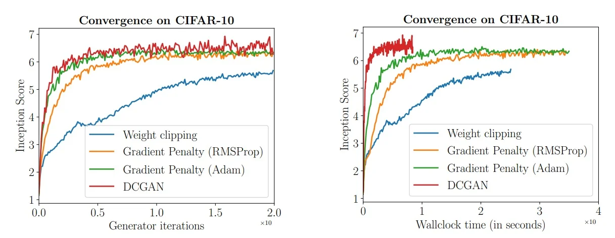
Architectural Robustness One of the most compelling benefits of WGAN-GP is its architectural flexibility. It works reliably with MLPs, DCGANs, and deep ResNets—even when using the same hyperparameters across models.
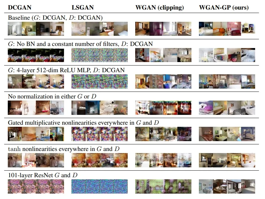
State-of-the-Art Results on CIFAR-10 (At the Time of Publication) In the experimental setup of Gulrajani et al. [201], WGAN-GP with a ResNet-based critic achieves leading Inception scores on CIFAR-10 among the compared unsupervised baselines at the time of publication. Since then, many subsequent GAN variants and training schemes have surpassed these numbers; here, the table is best read as evidence that stable Lipschitz enforcement enables higher-capacity architectures to train reliably and reach strong results under a fixed, controlled comparison.
| Unsupervised Model | Inception Score |
|---|---|
| ALI (Dumoulin et al.) | 5.34 \(\pm \) 0.05 |
| DCGAN (Radford et al.) | 6.16 \(\pm \) 0.07 |
| Improved GAN (Salimans et al.) | 6.86 \(\pm \) 0.06 |
| EGAN-Ent-VI | 7.07 \(\pm \) 0.10 |
| DFM | 7.72 \(\pm \) 0.13 |
| WGAN-GP (ResNet) | 7.86 \(\pm \) 0.07 |
Conclusion WGAN-GP combines the theoretical strength of optimal transport with the practical stability of smooth gradient regularization. It replaces rigid weight clipping with a principled, differentiable loss term—enabling deeper architectures, smoother convergence, and high-quality generation across domains. Its success laid the groundwork for many subsequent GAN improvements, including conditional models and progressive training techniques.
Enrichment 20.6: The StyleGAN Family
The StyleGAN family, developed by Karras et al. [289, 291, 290], represents a major advancement in generative modeling. These architectures build upon the foundational Progressive Growing of GANs (ProGAN) [293], introducing a radically different generator design that enables better disentanglement, fine-grained control, and superior image quality.
Enrichment 20.6.1: ProGAN Overview: A Stability-Oriented Design
ProGAN [293] stabilizes GAN training by progressively growing both the generator and discriminator during optimization. Instead of learning to synthesize \(1024\times 1024\) images from the start, training begins at a very low spatial resolution (typically \(4\times 4\)) and then doubles resolution in stages: \[ 4^2 \rightarrow 8^2 \rightarrow 16^2 \rightarrow \cdots \rightarrow 1024^2. \] The core idea is that early stages learn global structure (pose, layout, coarse shape) in a low-dimensional pixel space, while later stages specialize in high-frequency detail (texture, strands of hair, wrinkles), reducing optimization shock and improving stability.
Training Strategy ProGAN couples a resolution-aware curriculum with several stabilization heuristics (pixelwise feature normalization, minibatch standard deviation, equalized learning rate). The progressive schedule has two intertwined components: (i) architectural expansion and (ii) a fade-in transition that smoothly introduces newly added layers.
-
Progressive layer expansion (the core mechanism): To move from resolution \(R\) to \(2R\), ProGAN does not restart training from scratch. Instead, it grows both networks by appending a small, highest-resolution block while reusing the previously trained lower-resolution networks unchanged as an Old Stack. Conceptually, the Old Stack has already learned how to model and judge coarse structure at resolution \(R\), so the newly added parameters can concentrate on the incremental difficulty of handling finer-scale detail that only exists at resolution \(2R\). This isolates the new learning problem, reduces optimization shock, and makes the adversarial game substantially better conditioned.
-
Generator growth (adding detail at \(2R\)): Let \(G_R\) denote the generator after training at resolution \(R\). When run up to its last internal feature tensor, it produces \(h_R \in \mathbb {R}^{R \times R \times C}\), which encodes a stable coarse scene description (global pose, layout, low-frequency shape). To reach \(2R\), ProGAN upsamples this feature map and appends a New Block (typically two \(3\times 3\) convolutions) that operates specifically at the new resolution. Finally, a new toRGB head (a \(1\times 1\) convolution) projects the refined features to the three RGB channels: \[ \underbrace {z \to \cdots \to h_R}_{\substack {\mbox{Old Stack} \\ (R \times R \times C)}} \;\xrightarrow {\;\mbox{upsample}\;} \mathbb {R}^{2R\times 2R\times C} \;\xrightarrow [\substack {\mbox{New Block} \\ \mbox{(learns fine detail)}}]{\mbox{Two } 3\times 3 \mbox{ Convs}} h_{2R} \in \mathbb {R}^{2R\times 2R\times C'} \;\xrightarrow [\mathbf {1\times 1}]{\texttt{toRGB}} \underbrace {x_{2R}}_{\substack {\mbox{Output Image} \\ (2R \times 2R \times 3)}}. \] In practice, upsampling is performed via nearest-neighbor interpolation (to avoid checkerboard artifacts from transposed convolutions), followed by the two \(3\times 3\) convolutions.
The New Block and its toRGB head are the only components that must learn how to express and render the additional degrees of freedom available at \(2R\) (sharper edges, higher-frequency texture statistics), while the Old Stack continues to provide the already-learned global structure. This division of labor is the main reason progressive growing is easier to optimize than training a full \(2R\)-resolution generator from scratch, where global geometry and micro-texture would need to be discovered simultaneously under a rapidly strengthening discriminator.
-
Discriminator growth (mirroring the generator at \(2R\)): Let \(D_R\) denote the discriminator trained at resolution \(R\). At this point in training, \(D_R\) is already a competent “coarse realism” judge: it has learned to map an \(R\times R\) image (or, equivalently, an \(R\times R\) feature representation) to a scalar score by detecting global inconsistencies such as wrong layout, implausible shapes, or broken low-frequency statistics.
When we increase the generator’s output resolution to \(2R\), the discriminator must expand its perceptual bandwidth: it should still leverage its learned global judgment, but it must also become sensitive to the new high-frequency evidence that now exists in \(2R\times 2R\) images (e.g., sharper edges, texture regularities, aliasing artifacts). ProGAN achieves this without discarding the already-trained discriminator by growing the discriminator in the opposite direction of the generator: it prepends a small, high-resolution processing block at the input side, and then plugs the pre-trained \(D_R\) (the Old Stack) in after this new block.
Concretely, the new input-side block consists of a fromRGB stem (a \(1\times 1\) convolution) that lifts raw pixels into feature space, followed by two \(3\times 3\) convolutions that operate at resolution \(2R\) to analyze fine-detail cues, and finally an average-pooling downsample that produces an \(R\times R\) feature tensor of the shape expected by the old discriminator stack: \[ \underbrace {x_{2R}}_{\substack {\mbox{Input Image} \\ (2R \times 2R \times 3)}} \;\xrightarrow [\mathbf {1\times 1}]{\texttt{fromRGB}} \underbrace {\mathbb {R}^{2R\times 2R\times C'}}_{\substack {\mbox{High-res features} \\ \mbox{(new stem output)}}} \;\xrightarrow [\substack {\mbox{New Block} \\ \mbox{(critiques fine detail)}}]{\mbox{Two } 3\times 3 \mbox{ Convs}} \mathbb {R}^{2R\times 2R\times C} \;\xrightarrow {\;\mbox{avgpool}\;} \underbrace {\mathbb {R}^{R\times R\times C}}_{\substack {\mbox{Compatible input for} \\ \mbox{Old Stack } D_R}} \;\xrightarrow {\;D_R\;} \mbox{Score}. \]
This construction makes the training dynamics much better behaved. The old discriminator \(D_R\) is not “thrown away” and relearned; it remains intact and continues to process an \(R\times R\) representation with the same tensor shape and comparable semantic level as in the previous stage. In other words, the newly added high-resolution block acts as a learned front-end sensor: it observes the extra information available at \(2R\), extracts the fine-scale evidence that was previously invisible, and then hands a downsampled summary to the already-trained “global judge” \(D_R\).
As a result, the discriminator becomes stronger exactly where the generator gained new degrees of freedom, but it does so in a controlled, localized way: most of the discriminator’s capability (the Old Stack) remains a stable foundation for judging geometry and low-frequency structure, while only the new input-side block must learn how to interpret and penalize higher-frequency artifacts. This is one of the key reasons progressive growing improves stability compared to training a large \(2R\)-resolution discriminator from scratch, which can either (i) rapidly overpower the generator before it has learned coarse structure, or (ii) destabilize optimization by forcing the entire discriminator to simultaneously learn both global and fine-scale judgments from an initially weak generator distribution.
-
-
Fade-in mechanism (what is blended, when, and how it is controlled): Abruptly inserting new layers can destabilize training, because the discriminator suddenly receives higher-resolution inputs and the generator suddenly produces outputs through untrained weights. ProGAN avoids this by linearly blending two image pathways during a dedicated transition period.
At resolution \(2R\), the generator produces the final RGB image via: \[ x^{\mbox{out}}_{2R}(\alpha ) = \alpha \cdot x^{\mbox{high}}_{2R} + (1-\alpha )\cdot x^{\mbox{low}}_{2R}, \qquad \alpha \in [0,1], \] where:
- \(x^{\mbox{high}}_{2R}\) is the RGB output from the new block (upsample \(\rightarrow \) conv \(\rightarrow \) toRGB) at resolution \(2R\).
- \(x^{\mbox{low}}_{2R}\) is obtained by taking the previous stage output \(x_R \in \mathbb {R}^{R\times R\times 3}\) and upsampling it to \(2R\times 2R\) (using the same deterministic upsampling).
The discriminator uses a matching fade-in at its input: \[ \phi ^{\mbox{in}}_{2R}(\alpha ) = \alpha \cdot \phi ^{\mbox{high}}_{2R} + (1-\alpha )\cdot \phi ^{\mbox{low}}_{2R}, \] where \(\phi ^{\mbox{high}}_{2R}\) is the feature map after the new fromRGB and convs at \(2R\), and \(\phi ^{\mbox{low}}_{2R}\) is obtained by downsampling the input image to \(R\times R\) and passing it through the previous-stage fromRGB branch.
How \(\alpha \) is scheduled in practice: \(\alpha \) is treated as a deterministic scalar that is updated as training progresses, typically linearly with the number of images processed during the fade-in phase: \[ \alpha \leftarrow \min \!\left (1,\; \frac {n}{N_{\mbox{fade}}}\right ), \] where \(n\) is the number of training images seen so far in the fade-in phase and \(N_{\mbox{fade}}\) is a fixed hyperparameter (often specified in “kimg”). Equivalently, in code one updates \(\alpha \) once per minibatch using the minibatch size. After the fade-in phase completes (\(\alpha =1\)), ProGAN continues training at the new resolution for an additional stabilization phase with \(\alpha \) fixed to 1.
-
Stage completion criterion (schedule, not adaptive metrics): ProGAN uses a fixed curriculum, not an adaptive convergence test. Each resolution stage consists of:
- Fade-in phase: linearly ramp \(\alpha :0\rightarrow 1\) over \(N_{\mbox{fade}}\) images.
- Stabilization phase: continue training for \(N_{\mbox{stab}}\) images with \(\alpha =1\).
The values \(N_{\mbox{fade}},N_{\mbox{stab}}\) are resolution-dependent hyperparameters (often larger for high resolutions; e.g., hundreds of thousands of images per phase at \(128^2\) and above in the original setup).
- Upsampling and downsampling operators (why these choices): The generator uses nearest-neighbor upsampling followed by \(3\times 3\) convolutions to avoid the checkerboard artifacts often associated with transposed convolutions. The discriminator uses average pooling for downsampling to provide a simple, stable low-pass behavior, again followed by \(3\times 3\) convolutions.
Why This Works Progressive growing decomposes a difficult high-resolution game into a sequence of easier games:
- Large-scale structure first: At \(4^2\) or \(8^2\), the networks learn global layout with very limited degrees of freedom, reducing the chance that training collapses into high-frequency “noise wars” between generator and discriminator.
- Detail refinement later: Each new block primarily controls a narrower frequency band (finer scales), so it can specialize in textures while earlier blocks preserve global semantics.
- Compute efficiency: Early stages are much cheaper, and a substantial portion of training time occurs before reaching the largest resolutions, reducing total compute versus training exclusively at full resolution.
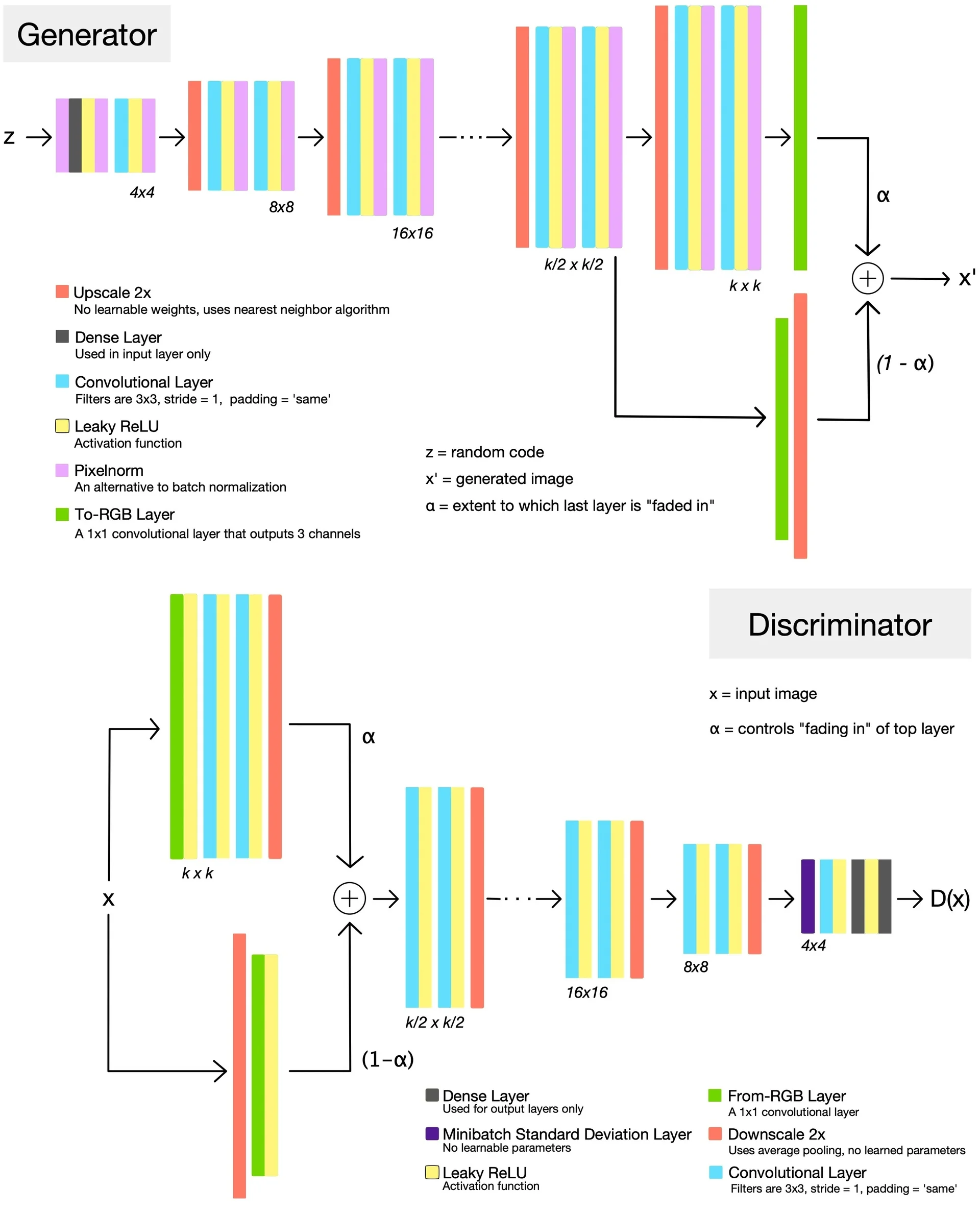
Stabilization Heuristics Beyond the progressive growth curriculum, ProGAN introduces three concrete modifications whose shared goal is to make the generator–discriminator game numerically well-conditioned: (i) keep generator signal magnitudes from drifting or “escalating” across depth and time, (ii) give the discriminator an explicit handle on within-batch diversity so collapse is easier to detect, and (iii) equalize the effective step sizes of different layers by a simple re-parameterization of convolution weights.
-
Pixelwise feature normalization (PixelNorm in the generator): ProGAN inserts a deterministic normalization step after each convolutional layer in the generator (in the original architecture, after the nonlinearity), applied independently at every spatial location and independently for every sample in the minibatch. Let \(a_{h,w} \in \mathbb {R}^{C}\) denote the channel vector at pixel \((h,w)\) in some intermediate generator feature map (for a fixed sample). PixelNorm rescales this vector by its root-mean-square (RMS) magnitude: \[ b_{h,w} = \frac {a_{h,w}}{\sqrt {\frac {1}{C}\sum _{j=1}^{C}\bigl (a_{h,w}^{(j)}\bigr )^2 + \epsilon }}, \qquad b_{h,w}\in \mathbb {R}^{C}. \] This operation has no batch dependence and no learnable affine parameters (no \(\gamma ,\beta \)); it is a pure, local rescaling.
Why this particular form helps. The generator repeatedly upsamples and refines features, so small imbalances in per-layer gain can amplify over depth, leading to layers that operate at very different dynamic ranges. PixelNorm acts as a per-location “automatic gain control”: it keeps the feature energy at each pixel close to a fixed scale, while still allowing the network to encode semantics in the direction of \(a_{h,w}\) (i.e., relative patterns across channels). This tends to reduce sensitivity to initialization and learning-rate choices, and it limits runaway signal magnitudes without forcing the generator to be linear or low-capacity.
How it differs from common normalizers. BatchNorm normalizes using minibatch statistics, coupling unrelated samples and potentially injecting batch-dependent artifacts into generation; PixelNorm avoids this entirely by operating per sample and per spatial location. LayerNorm typically uses both centering and scaling (subtracting a mean and dividing by a standard deviation over channels, sometimes over larger axes depending on implementation) and is usually paired with a learnable affine transform; PixelNorm performs only RMS-based rescaling (no mean subtraction) and no learned gain/shift, which preserves sparsity patterns induced by ReLU/leaky-ReLU and keeps the normalization as a lightweight stabilizer rather than a feature-wise affine re-mapping. In the ProGAN context, the intent is not “feature whitening” but simply keeping the generator’s internal signal scale under control throughout progressive growth.
-
Minibatch standard deviation (explicit diversity signal in the discriminator): Mode collapse is difficult for a standard discriminator to detect because it scores each image independently: if the generator outputs the same plausible-looking image for many latent codes, per-sample classification can remain ambiguous even though the set of samples is clearly non-diverse. ProGAN addresses this by appending a statistic that measures variation across the minibatch to the discriminator’s activations near the end of the network.
Computation. Let \(f \in \mathbb {R}^{N\times C\times H\times W}\) be a discriminator feature tensor for a minibatch of size \(N\) at some late layer (typically when spatial resolution is already small).
The minibatch standard deviation layer computes:
- (a)
- Batch-wise deviation: compute the per-feature, per-location standard deviation across the minibatch, \[ \sigma _{c,h,w} = \sqrt {\frac {1}{N}\sum _{n=1}^{N}\bigl (f_{n,c,h,w}-\mu _{c,h,w}\bigr )^2 + \epsilon }, \qquad \mu _{c,h,w}=\frac {1}{N}\sum _{n=1}^{N} f_{n,c,h,w}. \]
- (b)
- Aggregate to a scalar: average \(\sigma _{c,h,w}\) over channels and spatial positions to obtain a single scalar \(s\in \mathbb {R}\), \[ s = \frac {1}{CHW}\sum _{c,h,w}\sigma _{c,h,w}. \]
- (c)
- Broadcast and concatenate: replicate \(s\) to a constant feature map \(s\mathbf {1}\in \mathbb {R}^{N\times 1\times H\times W}\) and concatenate it as an additional channel: \[ f' = \mathrm {Concat}\bigl (f,\; s\mathbf {1}\bigr )\in \mathbb {R}^{N\times (C+1)\times H\times W}. \] How it is used inside the discriminator: the next discriminator layers simply continue operating on \(f'\) (now with \(C+1\) channels). In particular, the subsequent convolution (or final dense layers, depending on the stage) has trainable weights on this extra channel, so it can treat \(s\mathbf {1}\) as a dedicated “diversity sensor” and incorporate it into the real/fake decision alongside the usual learned features.
Why this discourages collapse. If the generator collapses so that samples in the batch become nearly identical, then many discriminator features also become nearly identical across \(n\), driving \(\sigma _{c,h,w}\) (and hence \(s\)) toward zero. The discriminator can then learn a simple rule: “real batches tend to exhibit non-trivial variation, whereas collapsed fake batches do not”. This converts lack of diversity into an easily separable cue, forcing the generator to maintain perceptible sample-to-sample variability in order to keep the discriminator uncertain. The aggregation to a single scalar is deliberate: it provides a robust, low-variance signal that is hard to game by injecting diversity into only a small subset of channels or spatial positions.
How this affects the generator (the feedback loop). Although \(s\) is computed inside the discriminator, it changes the generator’s training signal because the discriminator’s output now depends on a quantity that summarizes between-sample variation. During backpropagation, gradients flow from the discriminator score through the weights that read the extra channel \(s\mathbf {1}\), then through the computation of \(s\), and finally back to the generator parameters via the generated samples that contributed to \(f\). Consequently, if the discriminator learns to penalize low \(s\) as “fake”, the generator can only improve its objective by producing batches for which the discriminator features are not nearly identical across different latent codes. Operationally, this introduces a pressure to map different \(z\) values to meaningfully different outputs (and intermediate discriminator activations), counteracting the collapsed solution in which \(G(z_1)\approx G(z_2)\) for many \(z_1\neq z_2\).
-
Equalized learning rate (EqLR): Standard initializations (like He or Xavier) scale weights once at initialization to ensure stable signal magnitudes. However, this creates a side effect: layers with different fan-ins end up with weights of vastly different magnitudes (e.g., \(0.01\) vs \(1.0\)). Since modern optimizers (like Adam) often use a global learning rate, this leads to update speeds that vary wildly across layers. ProGAN solves this by decoupling the parameter scale from the signal scale.
The Mechanism (Runtime Scaling). First, recall that fan-in (\(n\)) is the number of input connections to a neuron (e.g., \(k^2 \cdot C_{in}\) for a convolution). In EqLR, we initialize all stored parameters \(w\) from a standard normal distribution \(\mathcal {N}(0, 1)\). Then, during every forward pass, we scale them dynamically: \[ w_{\mbox{effective}} = w \cdot c, \qquad \mbox{where } c = \sqrt {\frac {2}{n}}. \] The layer uses \(w_{\mbox{effective}}\) for convolution, ensuring the output activations have unit variance (just like He initialization).
Why this stabilizes training (The ”Learning Speed” Intuition). The benefit appears during the backward pass. To see why, compare a large layer (where weights must be small) under both schemes:
- Standard He Initialization: We initialize \(w \approx 0.01\). If the learning rate is \(\eta = 0.01\), a single gradient step can change the weight from \(0.01 \to 0.02\). This is a huge 100% relative change, causing the layer to train explosively fast and potentially diverge.
- EqLR: We initialize \(w \approx 1.0\). The constant \(c \approx 0.01\) handles the scaling downstream. Now, the same gradient update \(\eta = 0.01\) changes the stored parameter from \(1.0 \to 1.01\). This is a stable 1% relative change.
Result: By keeping all stored parameters in the same range (\(w \sim 1\)), EqLR ensures that all layers—regardless of their size—learn at the same relative speed. This prevents the ”race condition” where some layers adapt instantly while others lag behind, which is critical for the delicate balance of GAN training.
Note on Inference: There is no train–test discrepancy. The scaling \(c\) is a fixed mathematical constant derived from the architecture dimensions. It is applied identically during training and inference.
Enrichment 20.6.1.1: Limitations of ProGAN: Toward Style-Based Generators
While ProGAN successfully synthesized high-resolution images with impressive quality, its architecture introduced three fundamental limitations that StyleGAN sought to overcome:
- Latent code bottleneck: The latent vector \( z \sim \mathcal {N}(0, I) \) is injected only once at the input. Its influence can weaken in deeper layers, which are responsible for fine-grained texture and microstructure.
- Entangled representations: High-level attributes such as pose, identity, and background are mixed in the latent space, so small perturbations in \( z \) can produce unpredictable coupled changes across multiple factors.
- Lack of stochastic control: Fine-scale stochastic details (e.g., pores, hair microstructure, subtle lighting variation) are not explicitly controlled or reproducibly isolatable in the generator.
These limitations motivated a rethinking of the generator design—leading to StyleGAN, which introduces multi-resolution modulation, explicit stochastic inputs, and a non-linear mapping from \( z \) to intermediate style vectors to improve disentanglement and controllability.
Enrichment 20.6.2: StyleGAN: Style-Based Synthesis via Latent Modulation
While ProGAN succeeded in generating high-resolution images by progressively growing both the generator and discriminator, its architecture left a core limitation unresolved: the latent code \( z \sim \mathcal {N}(0, I) \) was injected only at the input layer of the generator. As a result, deeper layers — responsible for fine-grained details — received no direct influence from the latent space, making it difficult to control semantic factors in a disentangled or interpretable way.
StyleGAN, proposed by Karras et al. [289], addresses this by completely redesigning the generator, while keeping the ProGAN discriminator largely unchanged. The key idea is to inject the latent code — transformed into an intermediate vector \( w \in \mathcal {W} \) — into every layer of the generator. This turns the generator into a learned stack of stylization blocks, where each resolution is modulated independently by semantic information.
This architectural shift repositions the generator not as a direct decoder from latent to image, but as a controllable, hierarchical stylization process — enabling high-quality synthesis and fine-grained control over attributes like pose, texture, and color.
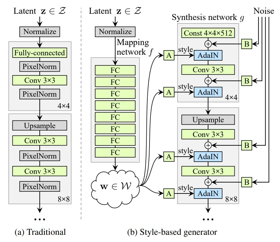
Key Architectural Ideas
(1) Mapping Network (\(\mathcal {Z} \to \mathcal {W}\)): Instead of injecting the latent vector \( z \in \mathbb {R}^d \) directly into the generator, StyleGAN introduces a learned mapping network — an 8-layer MLP that transforms \( z \) into an intermediate latent vector \( w = f(z) \in \mathcal {W} \). This design serves two main purposes:
- Alleviating entanglement (empirically): The original latent space \( \mathcal {Z} \) tends to entangle unrelated attributes — such as pose, hairstyle, and facial expression — making them difficult to control independently. The mapping network learns to reparameterize the latent space into \( \mathcal {W} \), which is observed (empirically) to be more disentangled: specific dimensions in \( w \) often correspond to localized and semantically meaningful variations.
- Improved editability: The intermediate latent space \( \mathcal {W} \) facilitates smoother interpolation and manipulation. Small movements in \( w \) tend to yield isolated, predictable image changes (e.g., adjusting skin tone or head orientation) without unintentionally affecting other factors.
Why Not Just Increase the Dimensionality of \( z \)? A natural question arises: could increasing the dimensionality of the original latent vector \( z \) achieve the same effect as using a mapping network? In practice, the answer is no — the limitation lies not in the capacity of \( z \), but in its geometry.
Latents drawn from \( \mathcal {N}(0, I) \) are distributed isotropically: all directions in \( \mathcal {Z} \) are equally likely, with no preference for meaningful directions of variation. This forces the generator to learn highly nonlinear transformations to decode useful structure from \( z \), often leading to entangled image features. Merely increasing the dimension expands the space without addressing this fundamental mismatch.
By contrast, the mapping network explicitly learns to warp \( \mathcal {Z} \) into \( \mathcal {W} \), organizing it such that different axes correspond more closely to semantically interpretable changes. While not theoretically guaranteed, this empirically observed disentanglement leads to significant improvements in image control, interpolation quality, and latent traversal. Karras et al. [289] demonstrate that using \( w \in \mathcal {W} \) consistently outperforms direct use of \( z \) — even with larger dimension — in terms of editability and semantic structure.
(2) Modulating Each Layer via AdaIN (Block A): In ProGAN, the latent code \(z\) is injected only once at the input. To prevent signal magnitude escalation, ProGAN uses PixelNorm, which forces every feature vector to unit norm. While stable, this is rigid: it applies the same normalization rule to every image, denying the latent code the ability to emphasize or suppress specific features sample-by-sample.
The Feature Statistics Hypothesis: What is “Style”? To understand StyleGAN’s solution, we must first define what “style” means in the context of Convolutional Neural Networks. Building on insights from neural style transfer [259], StyleGAN relies on the Feature Statistics Hypothesis:
- Spatial Layout (Content): The relative spatial locations of peaks and valleys in a feature map encode geometry (e.g., “an eye is at pixel \((10,10)\)”).
- Global Statistics (Style): The channel-wise mean and variance encode the texture or appearance (e.g., “how strong are the edges globally?” or “what is the background lighting?”).
Under this hypothesis, we can alter the “style” of an image simply by overwriting its feature map statistics, without needing to modify the spatial layout directly.
The “Wash and Paint” Mechanism (AdaIN). StyleGAN replaces PixelNorm with Adaptive Instance Normalization (AdaIN), turning each synthesis layer into a latent-controlled feature-styling module.
Unlike neural style transfer, which borrows statistics from a reference image, StyleGAN predicts the target statistics from the intermediate latent code \(w\). The operation proceeds in two steps:
Step 1: The Wash (Instance Normalization). First, we strip the input features of their current style statistics. Let \(x_\ell \in \mathbb {R}^{N \times C_\ell \times H_\ell \times W_\ell }\) be the activation tensor at layer \(\ell \). For each sample \(i\) and channel \(c\), we compute the spatial mean \(\mu \) and standard deviation \(\sigma \) across the dimensions \((H_\ell , W_\ell )\): \[ \mbox{Norm}(x_{\ell ,i,c}) = \frac {x_{\ell ,i,c} - \mu _{\ell ,i,c}}{\sigma _{\ell ,i,c}}. \] This “wash” removes the global energy and offset from the feature map while preserving its relative spatial structure. Ideally, the network retains where the features are (the layout), but forgets how strong they are.
Step 2: The Paint (Latent-Driven Modulation). Next, StyleGAN “paints” new statistics onto this canonical canvas. The latent \(w\) is projected via a learned affine transform \(A_\ell \) into style parameters: \[ (\gamma _\ell (w), \beta _\ell (w)) = A_\ell (w), \quad \gamma _\ell , \beta _\ell \in \mathbb {R}^{C_\ell }. \] These parameters are broadcast across the spatial dimensions \((H_\ell , W_\ell )\) to modulate the normalized features: \[ \mathrm {AdaIN}(x_\ell , w) = \underbrace {\gamma _\ell (w)}_{\mbox{Scale}} \odot \mbox{Norm}(x_\ell ) + \underbrace {\beta _\ell (w)}_{\mbox{Bias}}. \]
Why does this work? (Mathematical Derivation). We can prove that this operation forces the output features to have exactly the statistics dictated by \(w\). Let \(\hat {x} = \mbox{Norm}(x)\). By construction, its spatial mean is 0 and variance is 1. The statistics of the output \(y = \gamma \hat {x} + \beta \) are: \[ \mathbb {E}[y] = \mathbb {E}[\gamma \hat {x} + \beta ] = \gamma \mathbb {E}[\hat {x}] + \beta = \beta , \] \[ \sqrt {\mbox{Var}[y]} = \sqrt {\mbox{Var}[\gamma \hat {x} + \beta ]} = \sqrt {\gamma ^2 \mbox{Var}[\hat {x}]} = \gamma . \] Thus, for every layer \(\ell \), the pair \((\beta _\ell (w), \gamma _\ell (w))\) is precisely the layer’s “style”: it directly dictates the baseline and contrast of every feature channel.
Intuition: The “Global Control Panel” Analogy. Imagine each channel \(c\) is a specific feature detector (e.g., Channel 42 detects “vertical wrinkles”). The AdaIN parameters act as a global control panel for these detectors:
-
Scale \(\gamma _{\ell ,c}\) (The Volume Knob): This controls the gain or contrast.
- High \(\gamma \): The volume is up. The detector’s response is amplified. Deep, sharp wrinkles appear wherever the layout indicates.
- Low \(\gamma \): The volume is down. The feature is muted or washed out.
-
Bias \(\beta _{\ell ,c}\) (The Offset Slider): This controls the baseline presence.
- High \(\beta \): The feature is active everywhere (e.g., brightening the global lighting condition).
- Low \(\beta \): The feature is suppressed below the activation threshold.
Key Limitations: Spatially Uniform and Channel-Wise Control. While powerful, the AdaIN mechanism imposes two strict algebraic constraints on how the latent code \(w\) can influence the image:
- Spatially Uniform Control: The parameters \(\gamma _\ell (w)\) and \(\beta _\ell (w)\) are scalars that are broadcast over all spatial locations \((H_\ell , W_\ell )\). This means \(w\) cannot directly specify “brighten the top-left corner” differently from the bottom-right. It can only modulate the entire feature detector globally. (Note: Localized effects like a glint can still be produced via the spatial layout of the input features \(x_\ell \), but \(w\) cannot selectively target them).
- Channel-Wise (Diagonal) Control: The modulation acts on each channel independently. The affine transformation scales and shifts individual feature detectors but cannot mix or rotate them based on the latent code. Any coordination between channels must be handled implicitly by the convolutional weights.
The Downside: Normalization Artifacts (“Droplets”). These limitations—specifically the Instance Normalization step (The “Wash”)—are the primary motivation for StyleGAN2. Because AdaIN re-normalizes every feature map to unit variance, it discards the relative signal strength between channels. To bypass this, the generator learns to create localized spikes in signal magnitude (blobs or “droplets”) in the background. These spikes inflate the variance \(\sigma \), allowing the generator to manipulate the normalization constant and effectively preserve signal magnitude elsewhere. StyleGAN2 resolves this by removing explicit normalization in favor of a new weight demodulation scheme, which preserves the benefits of style modulation without causing these artifacts.
Why this matters (Hierarchical Control): Despite the limitation, this mechanism yields the disentanglement properties StyleGAN is famous for:
- Explicit separation of layout and appearance: The spatial arrangement flows through the convolutions (the “content”), while \(w\) acts as an external controller that overwrites the statistics (the “style”).
- Sample-dependent behavior: The same convolutional filters behave differently for different images because their operating points are modulated by \(w\).
- Coarse-to-fine control: By modulating early layers, \(w\) controls the statistics of coarse features (pose, shape). By modulating deeper layers, it controls fine details (colors, micro-textures).
(3) Fixed Learned Input (Constant Tensor): A second innovation in StyleGAN is the use of a fixed learned input tensor: a constant trainable block of shape \( 4 \times 4 \times C \), shared across all samples. Unlike earlier GANs, where \( z \) or \( w \) was reshaped into an initial feature map, StyleGAN treats this constant as a base canvas.
All variation is introduced after this tensor, via style-based AdaIN modulation and additive noise. This decoupling is only viable because AdaIN provides a mechanism to inject sample-specific statistics into every layer. Without such modulation, a fixed input would collapse to identical outputs; with AdaIN, global structure emerges from the constant canvas, while semantic and stylistic variation is progressively layered in.
This design enforces:
- Consistent spatial structure: A shared input encourages stable layouts (e.g., facial geometry), while variations arise from modulation.
- Stronger disentanglement: Since \( w \) no longer defines spatial structure, it can focus on semantic and appearance attributes.
(4) Stochastic Detail Injection (Block B): To introduce variation in fine-grained details, StyleGAN adds Gaussian noise per spatial location. A single-channel noise map is drawn from \( \mathcal {N}(0,1) \), broadcast across channels, scaled by learned per-channel strengths, and added: \[ x' = x + \gamma \cdot \mbox{noise}, \qquad \gamma \in \mathbb {R}^C. \] This stochastic injection (Block B) allows natural variability (e.g., freckles, hair strands) without affecting global style.
Together, Blocks A and B mark a conceptual shift. Instead of mapping latent codes directly into images, StyleGAN decomposes generation into:
- Global, semantic variation: style-modulated via affine AdaIN.
- Local, stochastic variation: injected via per-layer noise.
Summary of changes from the original AdaIN: In Huang & Belongie’s work, AdaIN is a non-parametric alignment of statistics between two images [259]. StyleGAN modifies it into a parametric operator: style statistics are no longer extracted but predicted from latent codes. This repurposing enables a constant input tensor, because all per-sample variation is reintroduced through AdaIN and noise.
(5) Style Mixing Regularization: Breaking Co-Adaptation Across Layers A key goal of StyleGAN is to enable disentangled, scale-specific control over the synthesis process: early generator layers should influence coarse structure (e.g., face shape, pose), while later layers refine medium and fine details (e.g., eye color, skin texture). This structured control relies on the assumption that styles injected at each layer should work independently of one another.
However, if the generator always receives the same latent vector \( w \in \mathcal {W} \) at all layers during training, it may fall into a form of co-adaptation: early and late layers jointly specialize to particular combinations of attributes (e.g., blond hair only appears with pale skin), resulting in entangled features and reduced diversity.
Style Mixing Regularization disrupts this overfitting by occasionally injecting two distinct styles into the generator during training:
- Two latent codes \( z_1, z_2 \sim \mathcal {Z} \) are sampled and mapped to \( w_1 = f(z_1) \), \( w_2 = f(z_2) \).
- At a randomly chosen resolution boundary (e.g., \(16 \times 16\)), the generator applies \( w_1 \) to all earlier layers and switches to \( w_2 \) for the later layers.
Why this works: Because the generator is trained to synthesize coherent images even when style vectors abruptly change between layers, it cannot rely on tight correlations across resolutions. Instead, each layer must learn to independently interpret its style input. For example:
- If early layers specify a round face and neutral pose (from \( w_1 \)), then later layers must correctly render any eye shape, hair color, or lighting (from \( w_2 \)), regardless of what \( w_1 \) “would have” dictated.
- This prevents the network from implicitly coupling attributes (e.g., enforcing that a certain pose always goes with a certain hairstyle), which helps achieve true scale-specific disentanglement.
Result: Style Mixing acts as a form of regularization that:
- Improves editing robustness, as individual \( w \) vectors can be manipulated without unexpected side effects.
- Enables style transfer and recombination, where coarse features can be swapped independently of fine features.
- Encourages the generator to learn modularity, treating layer inputs as semantically independent rather than jointly entangled.
(6) Perceptual Path Length (PPL): Quantifying Disentanglement in Latent Space One of the defining features of a well-disentangled generative model is that interpolating between two latent codes should cause predictable, semantically smooth changes in the generated output. To formalize this idea, StyleGAN introduces the Perceptual Path Length (PPL) — a metric designed to measure the local smoothness of the generator’s mapping from latent codes to images.
PPL computes the perceptual distance between two very close interpolated latent codes in \( \mathcal {W} \)-space. Specifically, for two samples \( w_1, w_2 \sim \mathcal {W} \), we linearly interpolate between them and evaluate the visual difference between outputs at a small step: \[ \mbox{PPL} = \mathbb {E}_{w_1, w_2 \sim \mathcal {W}} \left [ \frac {1}{\epsilon ^2} \cdot \mathrm {LPIPS}(G(w(\epsilon )) , G(w(0))) \right ], \quad w(\epsilon ) = (1 - \epsilon ) w_1 + \epsilon w_2, \] where \( \epsilon \ll 1 \) (e.g., \( \epsilon = 10^{-4} \)) and \( G(w) \) is the image generated from \( w \).
What Is LPIPS? The Learned Perceptual Image Patch Similarity (LPIPS) metric [800] approximates human-perceived visual differences by comparing the feature activations of two images in a pretrained deep network (e.g., VGG-16). Unlike pixel-wise distances, LPIPS captures semantic similarity (e.g., facial expression, lighting) and is insensitive to small, perceptually irrelevant noise. This makes it especially suitable for assessing smoothness in generated outputs.
Why PPL Matters — and How It Relates to Training PPL serves two key roles:
- Evaluation: A low PPL score implies that the generator’s mapping is smooth — small steps in \( \mathcal {W} \) lead to controlled, localized changes in the image. High PPL values, in contrast, signal entanglement — for example, where a minor shift might simultaneously change pose and hairstyle.
- Regularization (StyleGAN2): StyleGAN2 adds a path length regularization term that encourages consistent image changes per unit movement in \( \mathcal {W} \). This is implemented by randomly perturbing latent codes and penalizing variance in the image-space response, pushing the generator toward more linear and disentangled behavior.
Crucially, PPL also helps diagnose the effectiveness of the generator’s latent modulation mechanisms, including AdaIN and noise injection. Improvements in PPL correlate with better interpretability and higher-quality style control. In this sense, PPL provides a complementary lens to adversarial loss functions — it doesn’t measure realism per se, but rather semantic coherence under manipulation.
(7) Loss Functions: From WGAN-GP to Non-Saturating GAN + R1 While StyleGAN’s architecture is central to its performance, stable training dynamics are equally crucial. To this end, the authors explored two major loss formulations across different experiments and datasets:
- WGAN-GP [201] — used for datasets like CelebA-HQ and LSUN, following the ProGAN pipeline. This loss minimizes the Wasserstein-1 distance while enforcing 1-Lipschitz continuity of the critic via a soft gradient penalty on interpolated samples.
- Non-Saturating GAN with R1 Regularization [436] — used in more recent experiments with the FFHQ dataset. This formulation applies a gradient penalty only to real samples, improving local stability and enabling deeper generators to converge reliably. To reduce computational overhead, the penalty is often applied lazily (e.g., every 16 steps).
These loss functions are not mutually exclusive with the perceptual evaluation tools like PPL. In fact, StyleGAN’s most robust results — especially in FFHQ — combine:
- 1.
- R1-regularized non-saturating loss for stable GAN convergence,
- 2.
- Path length regularization to encourage disentangled and smooth latent traversals (i.e., low PPL),
- 3.
- And LPIPS-based evaluation for empirical disentanglement measurement.
Together, these tools enable StyleGAN to not only generate photorealistic images, but also produce consistent, interpretable, and user-controllable latent manipulations — a key departure from earlier GANs where realism and control often conflicted.
Summary and Additional Contributions Beyond its architectural innovations — such as intermediate latent modulation, per-layer AdaIN, and stochastic noise injection — StyleGAN owes part of its success to the introduction of the Flickr-Faces-HQ (FFHQ) dataset. Compared to CelebA-HQ, FFHQ offers higher quality and broader diversity in age, ethnicity, accessories, and image backgrounds, enabling more robust and generalizable training.
This combination of structural disentanglement and dataset diversity allows StyleGAN to generate not only high-fidelity images, but also provides fine-grained control over semantic and local attributes. These advances collectively position StyleGAN as a foundational step toward interpretable and high-resolution image synthesis.
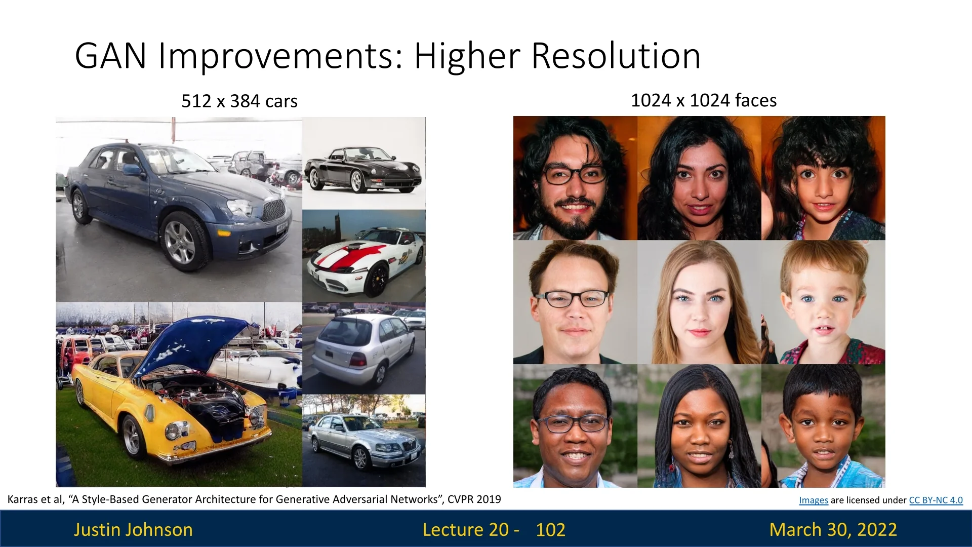
Emerging Capabilities
By separating global structure and local texture, StyleGAN enabled applications previously difficult in traditional GANs:
- Interpolation in latent space yields smooth, identity-preserving transitions.
- Truncation tricks can improve image quality by biasing \( w \) toward the center of \( \mathcal {W} \).
- Latent space editing tools can manipulate facial attributes with high precision.
This architectural shift — from latent vector injection to layer-wise modulation — laid the foundation for follow-up work on improved realism, artifact removal, and rigorous disentanglement.
Enrichment 20.6.3: StyleGAN2: Eliminating Artifacts, Improving Training Stability
StyleGAN2 [291] fundamentally refines the style-based generator framework, resolving key limitations of the original StyleGAN—most notably the so-called water droplet artifacts, excessive dependence on progressive growing, and training instabilities in high-resolution image synthesis. By removing or carefully restructuring problematic normalization modules, and by rethinking how noise and style manipulations are injected, StyleGAN2 achieves higher fidelity, improved consistency, and better disentanglement.
Enrichment 20.6.3.1: Background: From StyleGAN1 to StyleGAN2
StyleGAN1 (often termed StyleGAN1) introduced Adaptive Instance Normalization (AdaIN) in multiple generator layers, thereby allowing each feature map to be rescaled by learned style parameters. While this unlocked highly flexible style control and improved image quality, it also produced characteristic water droplet-like artifacts, most evident beyond \(64 \times 64\) resolution.
According to [291], the culprit lies in channel-wise normalization. AdaIN standardizes each feature map independently, removing not just its absolute magnitude but also any cross-channel correlations. In many cases, these correlations carry important relational information, such as spatial coherence or color harmony. By discarding them, the generator loses a mechanism to maintain consistent patterns across channels. In an effort to “sneak” crucial amplitude information forward, the network learns to insert extremely sharp, localized activation spikes. These spikes dominate the channel statistics at normalization time, effectively bypassing AdaIN’s constraints. Unfortunately, the localized spikes persist as structured distortions in the final images, creating the recognizable “droplet” effect.
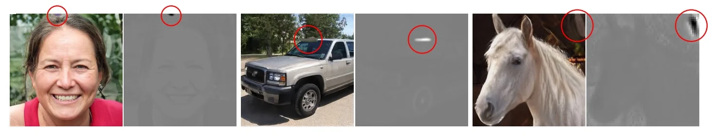
To resolve these issues, StyleGAN2 reexamines the generator’s foundational design. Rather than normalizing activations via AdaIN, it shifts style control to a weight demodulation paradigm, ensuring that channel relationships remain intact. By scaling weights before convolution, the generator can preserve relative magnitudes across channels and avoid the need for spurious spikes.
Beyond demodulation, StyleGAN2 also relocates noise injection, removes progressive growing, and employs new regularization strategies, leading to improved stability and sharper image synthesis. We outline these core innovations below.
Enrichment 20.6.3.2: Weight Demodulation: A Principled Replacement for AdaIN
Context and Motivation: In the original StyleGAN (StyleGAN1), each layer applied Adaptive Instance Normalization (AdaIN) to the activations post-convolution, enforcing a learned mean and variance on each channel. This eroded cross-channel relationships and caused the network to insert “activation spikes” to reintroduce lost amplitude information, giving rise to “droplet” artifacts. StyleGAN2 addresses this by normalizing the weights instead of the activations, thereby preserving channel coherence and eliminating those artifacts.
High-Level Flow in a StyleGAN2 Generator Block:
- 1.
- Input Feature Map and Style Code. Each block receives:
- The input feature map from the preceding layer (or from a constant input if it is the first block).
- A latent code segment \(\mathbf {w}_\mathrm {latent}\) specific to that layer, from the block A. In practice, \(\mathbf {w}_\mathrm {latent}\) is generated by an affine transform applied to \(\mathbf {W}\) (the style vector shared across layers, typically after a learned mapping network).
- 2.
- Optional Upsampling (Skip Generator): Before passing the feature map into the convolution, StyleGAN2 may upsample the spatial resolution if this block operates at a higher resolution than the previous one. In the simplified “skip-generator” design, upsampling occurs right before the convolution in each block (rather than as a separate training phase, as in progressive growing).
- 3.
- Weight Modulation: \[ w_{ijk}^{\prime } \;=\; s_i \,\cdot \, w_{ijk}, \quad \mbox{where } s_i = \mathrm {affine}\bigl (\mathbf {w}_\mathrm {latent}\bigr )_i. \] The style vector \(\mathbf {w}_\mathrm {latent}\) is used to generate a set of scale factors \(\{s_i\}\). These factors modulate (i.e., rescale) the convolution’s filter weights by channel \(i\). As a result, each channel’s influence on the output can be boosted or suppressed depending on the style.
- 4.
- Weight Demodulation: \[ w_{ijk}^{\prime \prime } \;=\; \frac {w_{ijk}^{\prime }}{\sqrt {\sum _{i}\sum _{k} \bigl (w_{ijk}^{\prime }\bigr )^2 + \varepsilon }}. \] After modulation, each output channel \(j\) is normalized so that the final “modulated+demodulated” filter weights \(\{w_{ijk}^{\prime \prime }\}\) remain in a stable range. Crucially, this step does not standardize the activations channel-by-channel; it only ensures that the overall filter magnitudes do not explode or vanish.
- 5.
- Convolution: \[ \mathrm {output} \;=\; \mathrm {Conv}\bigl (\mathrm {input},\, w^{\prime \prime }\bigr ). \] The network now applies a standard 2D convolution using the newly modulated-and-demodulated weights \(w_{ijk}^{\prime \prime }\). The resulting activations reflect both the incoming feature map and the style-dependent scaling, but without discarding cross-channel relationships.
Why This Avoids the Pitfalls of AdaIN.
- No Post-Activation Reset: Unlike AdaIN, where each channel’s mean/variance is forcibly re-centered, weight demodulation never re-normalizes each activation channel in isolation.
- Preserved Relative Magnitudes: Because the filters themselves incorporate style scaling before the convolution, the resulting activations can naturally maintain the relationships among channels.
- Prevents “Spikes”: The generator no longer needs to create sharp activation peaks to reintroduce magnitude differences lost by AdaIN’s normalization.
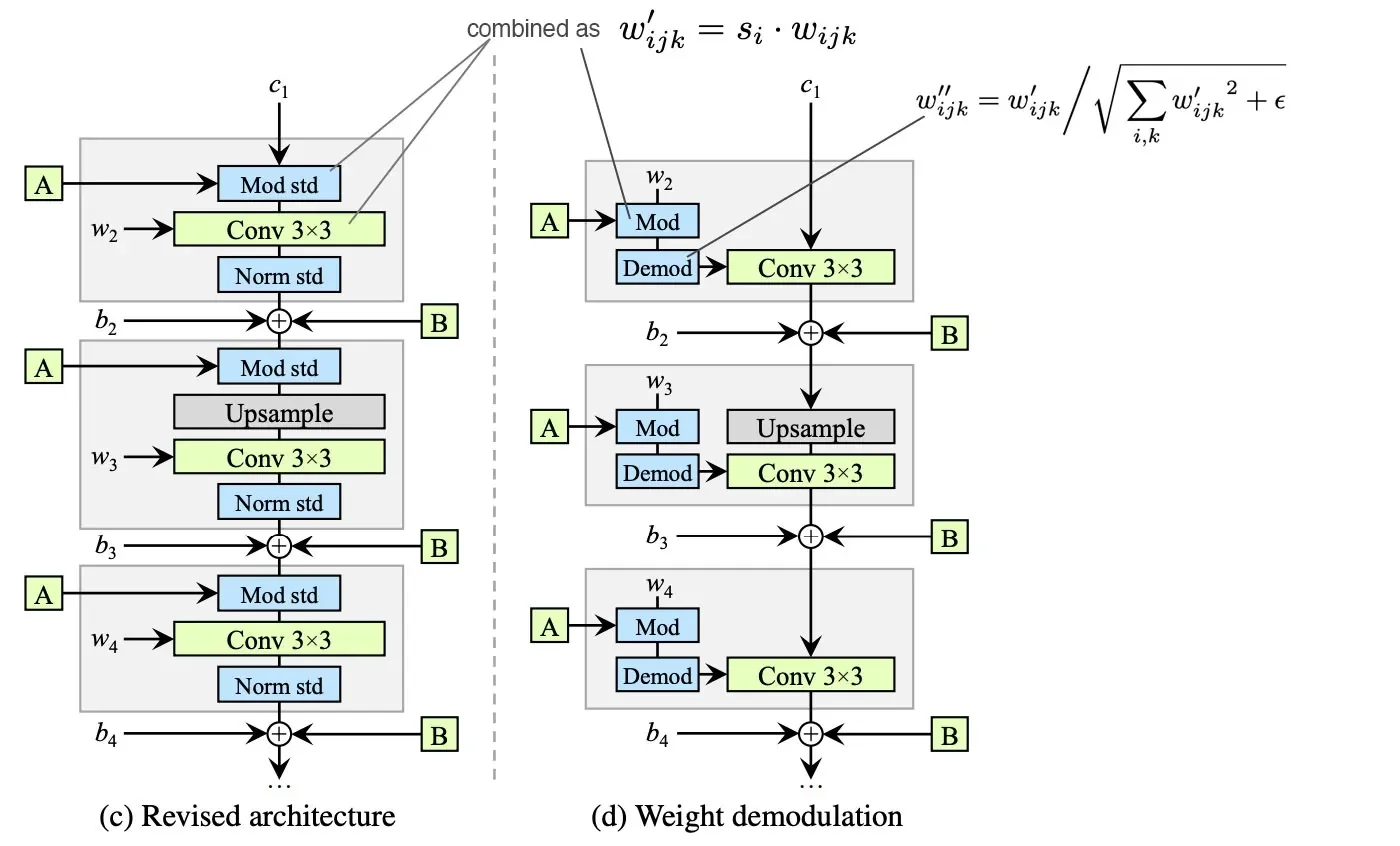
Maintaining Style Control: Even though the normalizing step moves from the activation space to the weight space, the style vector (\(\mathbf {w}_\mathrm {latent}\)) still dictates how each channel’s contribution is scaled. This ensures layer-wise flexibility over high-level attributes (e.g., color palettes, facial geometry, textures) without imposing uniform channel normalization. By avoiding activation-based standardization, StyleGAN2 preserves rich inter-channel information, thus enabling more stable and artifact-free synthesis.
Enrichment 20.6.3.3: Noise Injection Relocation: Separating Style and Stochasticity
In StyleGAN1, spatially uncorrelated Gaussian noise was injected within the AdaIN block — directly into normalized activations. This setup caused the style vector \( w \) and the random noise to interfere in ways that were hard to control. Because both types of signals shared the same normalization path, their effects were entangled, making it difficult for the generator to cleanly separate structured semantic features (e.g., pose, facial shape) from fine-grained randomness (e.g., freckles, skin pores).
StyleGAN2 resolves this by moving the noise injection outside the style modulation block. Now, the noise is added after convolution and nonlinearity, as a purely additive operation. This isolates noise from the style-driven modulation, allowing each component to play its role without interference:
- Noise: Adds per-pixel stochastic variation — capturing non-deterministic, high-frequency effects like hair placement, pores, or skin texture.
- Style (via \( w \)): Encodes global, perceptual properties such as pose, identity, and illumination.
By decoupling noise from normalization, the generator gains more precise control over where and how randomness is applied. This reduces unintended amplification of pixel-level variation, improves training stability, and enhances interpretability of the learned style representation.
Enrichment 20.6.3.4: Path Length Regularization: Smoother Latent Traversals
While StyleGAN1 introduced the perceptual path length (PPL) as a metric — using LPIPS [800] to quantify how much the image changes under latent interpolation — StyleGAN2 builds on this idea by turning it into a regularization objective. Crucially, however, the authors abandon LPIPS (which depends on pretrained VGG features) and instead compute the gradient directly in pixel space.
Why the change? Although LPIPS correlates well with human perception, it has several drawbacks when used for regularization:
- It is computationally expensive and requires forward passes through large pretrained networks (e.g., VGG16).
- It is non-differentiable or inefficient to backpropagate through, complicating training.
- It introduces a mismatch between the generator and the external perceptual model, which may bias optimization in unintended ways.
Instead, StyleGAN2 proposes a simpler yet effective solution: directly regularize the Jacobian norm of the generator with respect to the latent vector \( \mathbf {w} \in \mathcal {W} \), computed in pixel space. The goal is to ensure that small perturbations in latent space result in proportionally smooth and stable changes in the image. The proposed path length regularization loss is: \[ \mathcal {L}_\mbox{path} = \mathbb {E}_{\mathbf {w}, \mathbf {y}} \left [ \left ( \left \| \nabla _{\mathbf {w}} G(\mathbf {w}) \cdot \mathbf {y} \right \|_2 - a \right )^2 \right ], \] where:
- \( \mathbf {y} \sim \mathcal {N}(0, I) \) is a random direction in latent space.
- \( a \) is a running average of the expected gradient norm, which centers the loss to avoid shrinking gradients to zero.
Benefits of this formulation:
- Lightweight: No need to rely on external networks or pretrained feature extractors.
- Differentiable: The pixel-space gradient is fully backpropagatable through the generator.
- Tightly coupled to training: The regularization adapts directly to the generator’s own dynamics and feature statistics.
Although pixel-space distances are not perfectly aligned with human perception (as LPIPS aims to be), as it turns out, this gradient-based regularizer effectively captures smoothness in practice. It ensures that the generator’s output changes at a steady rate along latent directions, leading to better interpolations and more reliable latent editing.
Outcome: Latent walks in StyleGAN2 produce continuous, identity-preserving morphs with reduced topological discontinuities — a key improvement over the sometimes jerky transitions seen in StyleGAN1. This lightweight regularizer thus preserves the spirit of perceptual path length while avoiding its practical limitations.
Enrichment 20.6.3.5: Lazy R1 Regularization and Evolved Loss Strategy
StyleGAN1 explored a mix of loss strategies, including Wasserstein loss with gradient penalty (WGAN-GP) [201] and the non-saturating GAN loss with R1 regularization [436]. StyleGAN2 formalizes and stabilizes this setup, adopting a consistent combination of:
- Non-saturating GAN loss for both generator and discriminator.
- Lazy one-sided gradient penalty (R1) on real samples.
- Optional path length regularization on the generator.
Discriminator Loss: The full discriminator objective is given by: \[ \mathcal {L}_{D} = - \mathbb {E}_{x \sim p_{\mbox{data}}}[\log D(x)] - \mathbb {E}_{\tilde {x} \sim p_G}[\log (1 - D(\tilde {x}))] + \delta (i \boldsymbolod N = 0) \cdot \frac {\gamma }{2} \cdot \mathbb {E}_{x \sim p_{\mbox{data}}} \left [ \|\nabla _x D(x)\|_2^2 \right ], \] where the final term is the R1 gradient penalty, applied only every \(N\) steps (typically \(N = 16\)) to reduce computational overhead.
Generator Loss: The generator minimizes the standard non-saturating loss: \[ \mathcal {L}_G = - \mathbb {E}_{\tilde {x} \sim p_G}[\log D(\tilde {x})] + \lambda _{\mbox{path}} \cdot \mathcal {L}_{\mbox{path}}, \] where \(\mathcal {L}_{\mbox{path}}\) is the path length regularization term: \[ \mathcal {L}_{\mbox{path}} = \mathbb {E}_{\mathbf {w}, \mathbf {y}} \left [ \left ( \left \| \nabla _{\mathbf {w}} G(\mathbf {w}) \cdot \mathbf {y} \right \|_2 - a \right )^2 \right ], \] with \(\mathbf {y} \sim \mathcal {N}(0, I)\) and \(a\) a running exponential average of gradient magnitudes.
Joint Optimization Logic: Despite having different loss functions, the generator \(G\) and discriminator \(D\) are trained alternatingly in an adversarial setup:
- In each training iteration, the discriminator is first updated to better distinguish real samples \(x\) from generated ones \(\tilde {x} = G(\mathbf {w})\), using \(\mathcal {L}_D\).
- Then, the generator is updated to fool the discriminator, i.e., to maximize \(D(\tilde {x})\), via \(\mathcal {L}_G\).
- Regularization terms like R1 and path length are applied at different frequencies to avoid computational bottlenecks.
This adversarial training loop leads both networks to co-evolve: the generator learns to produce realistic images, while the discriminator sharpens its ability to detect fake ones — with each providing a learning signal to the other.
Why this setup works:
- R1 avoids the interpolation overhead of WGAN-GP while regularizing gradients only near real data points.
- Lazy application of both R1 and \(\mathcal {L}_{\mbox{path}}\) allows training to scale to higher resolutions without excessive cost.
- Path length regularization improves the smoothness and predictability of the generator’s latent-to-image mapping, aiding inversion and editing tasks.
Takeaway: StyleGAN2’s adversarial training framework and especially its modular loss design — non-saturating adversarial loss, lazy R1, and optional path regularization — has become the de facto foundation for modern high-resolution GANs.
Enrichment 20.6.3.6: No Progressive Growing
Moving Away From Progressive Growing. In ProGAN and StyleGAN1, progressive growing gradually adds higher-resolution layers during training, aiming to stabilize convergence and manage memory. Despite its initial success, this approach can fix early spatial layouts in ways that cause phase artifacts, such as misaligned facial geometry (e.g., teeth remain centered to the camera rather than following the head pose). These artifacts emerge because the network’s lower-resolution layers hard-code specific spatial assumptions that later layers struggle to correct.
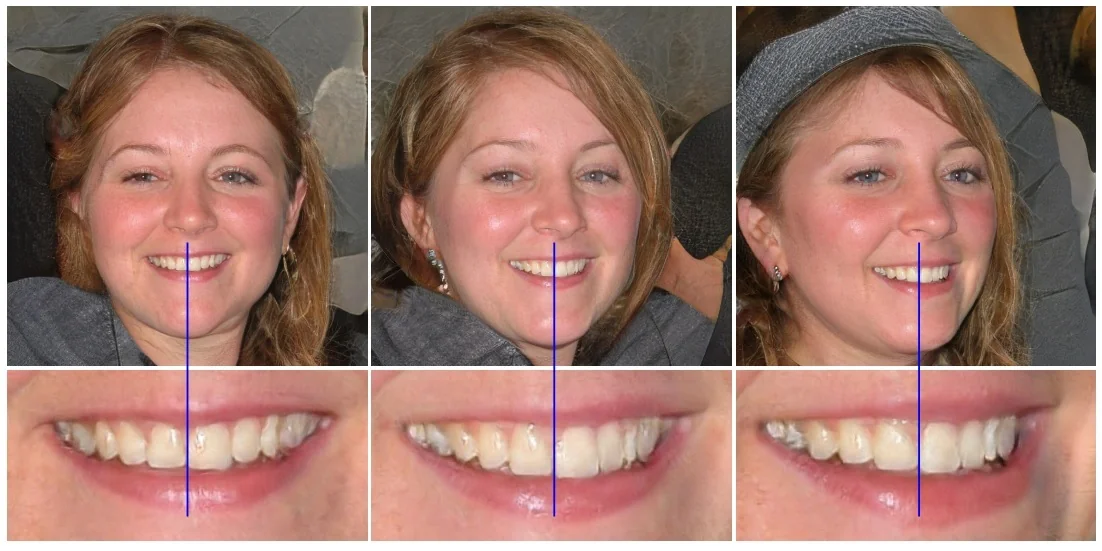
StyleGAN2 addresses these issues by removing progressive growing entirely and training directly at the target resolution from the outset. The architecture achieves the same coarse-to-fine benefits through more transparent and robust mechanisms:
1. Multi-Scale Skip Connections in the Generator
- RGB at Every Resolution. Each generator block outputs an RGB image at its own resolution (e.g., \(8 \times 8,\ 16 \times 16,\ \ldots ,\ 1024 \times 1024\)). These partial images are upsampled and summed to form the final output.
- Coarse to Fine in a Single Pass. Early in training, low-resolution blocks dominate the composite image, while higher-resolution blocks contribute less. As the network learns, the high-resolution outputs become more significant, refining details.
- No Opaque Fade-Ins. Instead of abruptly fading in new layers, each resolution’s contribution smoothly increases as training progresses, maintaining consistent alignment.
2. Residual Blocks in the Discriminator
- Residual Connections. The StyleGAN2 discriminator adopts a residual design, allowing inputs to bypass certain convolutions through identity (or \(1 \times 1\)) paths.
- Smooth Gradient Flow. The shortcut paths let gradients propagate effectively, even in early training, before higher-resolution features are fully meaningful.
- Flexible Depth Usage. Over time, the network learns to leverage high-resolution filters more, while the early residual connections remain available for coarse discrimination.
3. Tracking Per-Resolution Contributions The authors in [291] analyze how each resolution block affects the final output by measuring the variance of its partial RGB contribution through training. They observe:
- Early Dominance of Low-Res Layers. Initially, low-res blocks define major global structures.
- Increasing Role of High-Res Layers. As learning continues, high-resolution blocks (especially those with more channels) add finer details and sharper edges.
- Adaptive Shift Toward Detail. The model naturally transitions from coarse shapes to intricate textures without any manual “fade-in” scheduling.
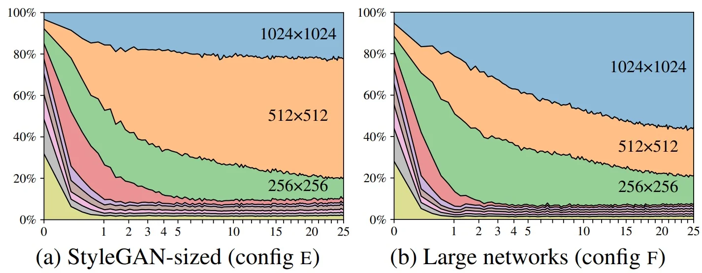
Why This Redesign Matters
- Avoids Locked-In Artifacts. Without progressive growing, low-resolution layers no longer imprint rigid spatial biases that cause geometry misalignment.
- All Layers Co-Adapt. The network learns to distribute coarse and fine features simultaneously, improving semantic consistency.
- Sharper and More Stable. Multi-resolution skip connections and residual blocks make training smoother, boosting final image fidelity and detail.
- Scalable to Deep/High-Res Models. Eliminating progressive phases simplifies training when moving to ultra-high resolutions or deeper networks.
Overall, StyleGAN2’s skip+residual generator and discriminator retain the coarse-to-fine advantage of progressive growing without succumbing to phase artifacts. This shift enables more stable training and sharper, better-aligned outputs at high resolutions.
Enrichment 20.6.3.7: StyleGAN3: Eliminating Texture Sticking
StyleGAN2 excels at photorealistic image synthesis but suffers from a subtle defect: texture sticking. When performing latent interpolations or spatial transformations (e.g., translation, rotation), textures like hair or skin do not follow the global object motion. Instead, they appear anchored to fixed pixel coordinates, leading to a breakdown of equivariance—the property that image content transforms consistently with object movement.
StyleGAN3 [290] re-engineers the entire generator pipeline to ensure alias-free behavior, eliminating unintended pixel-grid reference points that cause sticking. This is achieved by treating feature maps as bandlimited continuous signals and filtering all frequency components throughout the model. As a result, StyleGAN3 generates content that moves smoothly under sub-pixel shifts and rotations, making it suitable for video, animation, and neural rendering applications.
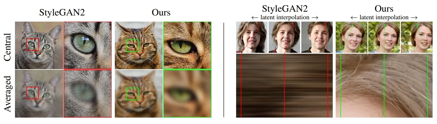
Why Does Texture Sticking Occur? The root cause lies in how the generator in StyleGAN2 implicitly uses positional information—especially during upsampling and convolution—introducing unintentional alignment with the image grid. The generator effectively creates textures based on pixel coordinates, not object-relative positions. This limits spatial generalization and causes artifacts when the generator is expected to simulate camera motion or rotation.
How StyleGAN3 Fixes It: Core Innovations
- 1.
- Bandlimited Filtering at All Resolutions: In earlier architectures, upsampling operations (e.g., nearest-neighbor, bilinear) introduced high-frequency artifacts by duplicating or interpolating values without controlling the spectral content. These artifacts then propagated through the network, causing textures to become “anchored” to pixel grid positions. StyleGAN3 resolves this by replacing standard up/downsampling with windowed sinc filters—true low-pass filters designed to attenuate high-frequency components beyond the Nyquist limit. The filter parameters (e.g., cutoff frequency, transition bandwidth) are tuned per resolution level to retain only the frequencies that the current scale can represent reliably. This ensures that spatial detail is consistent and alias-free across all scales.
- 2.
- Filtered Nonlinearities: Pointwise nonlinearities like LeakyReLU are known to introduce sharp spectral edges, generating high-frequency harmonics even when their inputs are smooth. These harmonics can cause aliasing when passed into lower-resolution branches or subsequent convolutions. StyleGAN3 inserts a filtering step around each nonlinearity: \[ \mbox{Upsample} \;\rightarrow \; \mbox{Activate} \;\rightarrow \; \mbox{Low-pass Filter} \;\rightarrow \; \mbox{Downsample}. \] This structure ensures that the nonlinear transformation doesn’t introduce frequency components that cannot be represented at the given resolution. As a result, each block only processes and propagates bandlimited signals, preserving translation and rotation equivariance throughout the network.
- 3.
- Fourier Feature Input and Affine Spatial Transforms: In StyleGAN2, the generator begins from a fixed, learnable \( 4 \times 4 \) tensor, which is inherently tied to the pixel grid. This gives the network a built-in “origin” and orientation, which can subtly leak positional information into the generated image. StyleGAN3 replaces this with a set of Fourier features—spatially continuous sinusoidal patterns encoding different frequencies. These features are not fixed but undergo an affine transformation (rotation and translation) controlled by the first latent vector \( \mathbf {w}_0 \). This change removes the generator’s reliance on the pixel grid and introduces a trainable coordinate system based on object geometry. As a result, spatial operations (like rotating or translating the input) correspond to smooth, meaningful changes in the generated image, supporting equivariant behavior even under subpixel movements.
- 4.
- Equivariant Kernel Design: In rotationally equivariant variants (e.g., StyleGAN3-R), convolutions are restricted to \(1 \times 1\) or radially symmetric kernels, ensuring that learned filters do not introduce directionality or grid-aligned bias.
- 5.
- No Skip Connections or Noise Injection: Intermediate skip-to-RGB pathways and stochastic noise injection are removed, both of which previously introduced fixed spatial bias. Instead, StyleGAN3 allows positional information to flow only via controlled transformations.
Training Changes and Equivariance Goals
- The Perceptual Path Length regularization (\(\mathcal {L}_\mbox{path}\)) from StyleGAN2 is removed, since it penalizes motion-equivariant generators by enforcing consistent change magnitudes in pixel space.
- StyleGAN3 achieves translation equivariance in the “T” configuration and rotation+translation equivariance in “R”. This makes it ideal for unaligned datasets (e.g., FFHQ-Unaligned) and motion synthesis.
Latent and Spatial Disentanglement While StyleGAN3 retains the original \( \mathcal {W} \) and StyleSpace (\( \mathcal {S} \)) representations, studies (e.g., [3]) show that:
- Editing in \(\mathcal {S}\) remains the most disentangled.
- Unaligned generators tend to entangle pose with other attributes, so pseudo-alignment (fixing \(w_0\)) or using an aligned generator with explicit spatial transforms (\(r, t_x, t_y\)) is recommended for editing.
- In videos: Texture sticking is almost entirely gone. Hairs, wrinkles, and facial features follow object movement.
- In interpolation: Latent traversals produce realistic and continuous changes, even under subpixel jitter.
- In inversion and editing: Real images can be reconstructed and manipulated with higher spatial coherence using encoders trained on aligned data and StyleGAN3’s affine spatial parameters.
Official code and models: https://github.com/NVlabs/stylegan3
Takeaway StyleGAN3 resolves one of the most persistent issues in GAN-generated motion: positional artifacts caused by grid alignment. Through a careful redesign grounded in signal processing, it enables truly equivariant, high-quality, and temporally consistent image generation—laying the foundation for advanced video editing, scene control, and neural rendering.
Enrichment 20.7: Conditional GANs: Label-Aware Image Synthesis
Conditional GANs (cGANs) [448] enhance the classic GAN framework by incorporating structured inputs—such as class labels—into both the generator and discriminator. The motivation is clear: standard GANs produce samples from a learned distribution without any explicit control. If one wants to generate, say, only images of cats or digit “3” from MNIST, standard GANs offer no direct way to enforce that condition.
By injecting label information, cGANs enable class-conditional synthesis. The generator learns to produce samples \( G(z \mid y) \) that match a desired label \(y\), while the discriminator learns to assess whether a given sample is both real and label-consistent. This label-aware feedback significantly enhances training signals and improves controllability, quality, and diversity of generated samples.
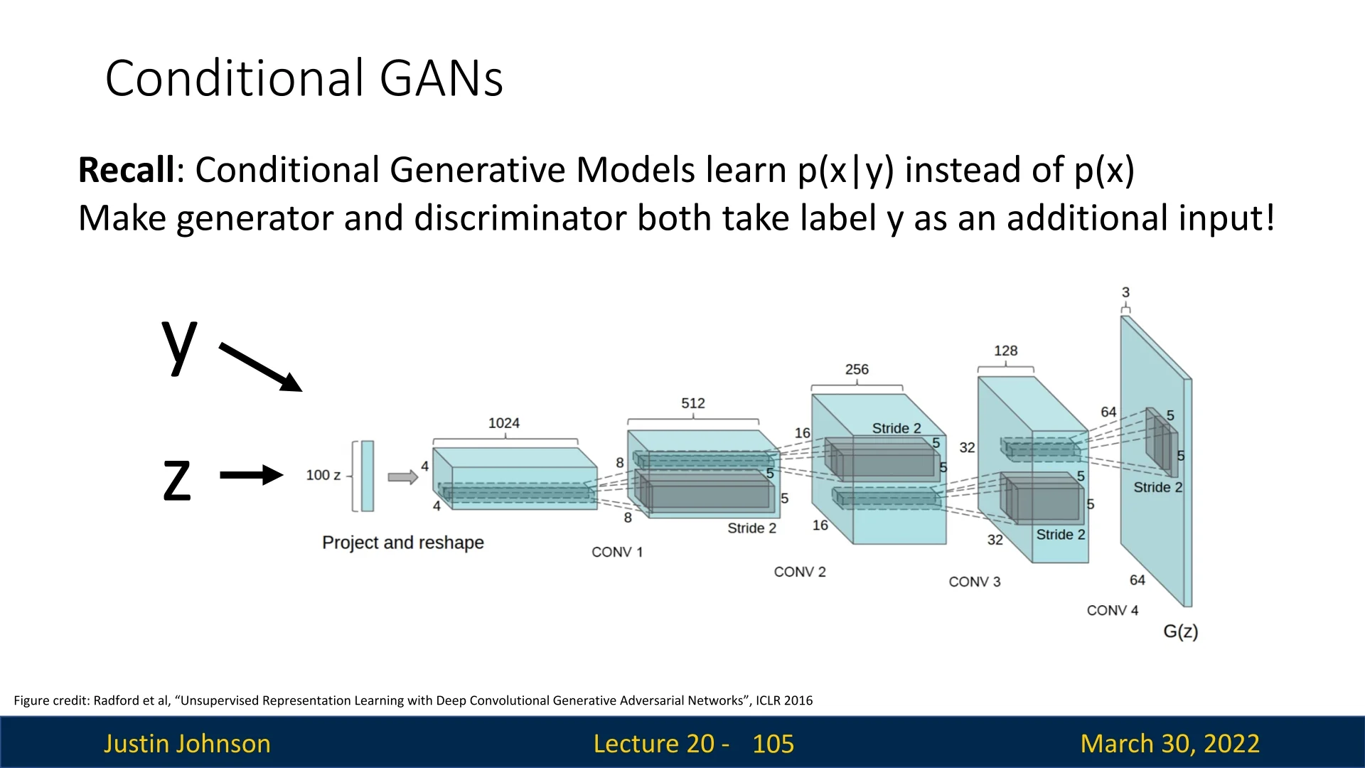
Enrichment 20.7.1: Conditional Batch Normalization (CBN)
Conditional Batch Normalization (CBN) [137] is a key technique that enables GANs to incorporate class information not just at the input level, but deep within the generator’s layers. Unlike naive conditioning methods—such as concatenating the label vector \( y \) with the latent code \( z \)—CBN injects label-specific transformations throughout the network, significantly improving class control and generation quality.
Motivation In the vanilla GAN setup, the generator learns a mapping from noise \( z \) to image \( x \), i.e., \( G(z) \approx x \). But what if we want \( G(z \mid y) \approx x_y \), an image from a specific class \( y \)? Concatenating \( y \) with \( z \) only conditions the generator’s first layer. What happens afterward is left unregulated—there is no guarantee that the network will retain or meaningfully use the label signal. This is especially problematic in deep generators. CBN solves this by embedding the label \( y \) into every normalization layer of the generator.
This ensures that class information continually modulates the internal feature maps across layers, guiding the generation process at multiple scales.
How CBN Works Let \( x \) be the input feature map to a BatchNorm layer. In standard BatchNorm, we normalize and then apply learned scale and shift: \[ \mathrm {BN}(x) = \gamma \cdot \frac {x - \mu }{\sigma } + \beta \]
CBN replaces the static \( \gamma \) and \( \beta \) with label-dependent values \( \gamma _y \) and \( \beta _y \), often produced via a small embedding or MLP based on \( y \): \[ \mathrm {CBN}(x \mid y) = \gamma _y \cdot \frac {x - \mu }{\sigma } + \beta _y \]
Here, each class \( y \) learns its own affine transformation parameters. This leads to class-specific modulation of normalized features—effectively injecting semantic ”style” throughout the generator.
- CBN allows for a shared generator backbone, with only minor per-class differences through \( \gamma _y \) and \( \beta _y \).
- During training, these class-specific affine parameters are learned jointly with the generator weights.
- CBN does not increase the number of convolutions but dramatically boosts the expressiveness of conditional generation.
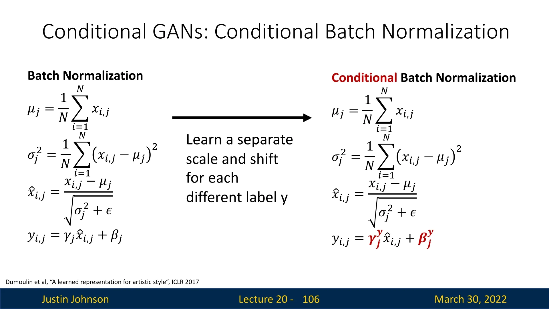
CBN in the Generator Conditional Batch Normalization (CBN) introduces class information deep into the generator. At each layer \( \ell \), the activations are batch-normalized and then rescaled using label-specific parameters \( \gamma _y^\ell \), \( \beta _y^\ell \), allowing each class to modulate the feature flow independently across scales.
Enrichment 20.7.1.1: Projection-Based Conditioning in Discriminators
While Conditional Batch Normalization (CBN) is highly effective for injecting label information into the generator, it is rarely applied in the discriminator. The discriminator’s primary responsibility is to distinguish real from fake images and verify that they match the target label \( y \). Rather than applying class-specific transformations to every layer, conditional information is typically injected via architectural conditioning, using either:
- Concatenation-Based Conditioning: The one-hot label \( y \) is spatially expanded and concatenated to the input image \( x \in \mathbb {R}^{3 \times H \times W} \), resulting in a combined tensor \( [x; y'] \in \mathbb {R}^{(3+C) \times H \times W} \), where \( C \) is the number of classes. While simple, this method weakens in deeper layers, where the label signal may vanish.
-
Projection Discriminator [451]: A more robust alternative that introduces label conditioning directly into the discriminator’s output logit. The logit is defined as: \[ \underbrace {D(x, y)}_{\mbox{class-aware score}} = \underbrace {b(x)}_{\mbox{realism term}} + \underbrace {h(x)^\top e(y)}_{\mbox{semantic match}}, \] where:
- \( h(x) \in \mathbb {R}^d \) is a global feature vector extracted from the image (after convolution and pooling).
- \( e(y) \in \mathbb {R}^d \) is a learned embedding vector for the class label \( y \).
- \( b(x) = w^\top h(x) \) is a standard linear layer predicting the realism of \( x \), independent of label.
This design cleanly separates visual quality from semantic alignment.
Advantages of Projection-Based Conditioning:
- Efficiency: Requires only one additional dot product at the final layer, with minimal parameter overhead.
- Interpretability: Clearly decomposes the output into realism and semantic compatibility terms.
- Scalability: Works well for large-scale datasets and deep discriminators (e.g., BigGAN which we’ll cover later).
By combining this strategy with techniques like Spectral Normalization (discussed next), projection-based discriminators remain stable even under high capacity settings and offer strong guidance for conditional image synthesis.
Enrichment 20.7.1.2: Training Conditional GANs with CBN
Conditional GANs (cGANs) trained with Conditional Batch Normalization (CBN) aim to synthesize images that are not only visually realistic, but also semantically aligned with a given class label \( y \). To achieve this, the generator and discriminator are trained in tandem, each using label information differently.
Generator \( G(z, y) \): Label-Aware Synthesis The generator receives a latent code \( z \sim \mathcal {N}(0, I) \) and a class label \( y \). The label modulates every normalization layer via CBN: \[ \mathrm {CBN}(x \mid y) = \gamma _y \cdot \frac {x - \mu }{\sigma } + \beta _y \] This injects label-specific transformations into the generator’s internal feature maps, allowing class control at multiple spatial scales. The output image is: \[ \tilde {x} = G(z, y) \]
Discriminator \( D(x, y) \): Realness and Label Consistency The discriminator receives both an image \( x \) and its associated label \( y \), and outputs a scalar score that jointly reflects:
- Whether the image looks real (i.e., sampled from \( p_{\mbox{data}} \) rather than the generator).
- Whether it is semantically consistent with the provided label \( y \).
This dual-role is often realized using a projection discriminator [451], where the label is embedded and combined with the discriminator’s internal features:
\[ D(x, y) = b(x) + h(x)^\top e(y) \]
Here, \( h(x) \) is a learned feature embedding from the image, \( e(y) \) is the learned embedding of the label \( y \), and \( b(x) \) is a base logit representing the visual realism of \( x \). The dot product term encourages semantic agreement between the image and the label — if \( h(x) \) and \( e(y) \) align well, \( D(x, y) \) increases.
Training Pipeline with CBN Conditioning: The Conditional GAN training loop is fully differentiable and jointly optimizes two objectives: (1) realism — fooling the discriminator into classifying fake images as real, and (2) semantic alignment — ensuring that generated images match the assigned class label. Conditional Batch Normalization (CBN) plays a key role in achieving this alignment by embedding the label \( y \) throughout the generator.
- 1.
- Sample Inputs: For each batch:
- Sample latent codes \( z^{(i)} \sim \mathcal {N}(0, I) \) and corresponding labels \( y^{(i)} \in \{1, \dots , K\} \).
- 2.
- Generate Conditioned Fakes: For each \( (z^{(i)}, y^{(i)}) \), generate a fake image: \[ \tilde {x}^{(i)} = G(z^{(i)}, y^{(i)}) \] The generator uses CBN at every layer to condition on \( y^{(i)} \), ensuring class-relevant features are injected at all depths.
- 3.
- Discriminator Update:
- For real images \( x^{(i)} \sim p_{\mbox{data}}(x \mid y^{(i)}) \), the discriminator \( D(x^{(i)}, y^{(i)}) \) should output a high value, indicating high confidence that the image is real and belongs to class \( y^{(i)} \).
- For fake images \( \tilde {x}^{(i)} \), the discriminator \( D(\tilde {x}^{(i)}, y^{(i)}) \) should output a low value, identifying them as generated (and potentially misaligned with \( y^{(i)} \)).
- 4.
- Loss Functions:
- Discriminator: \[ \mathcal {L}_D = -\frac {1}{N} \sum _{i=1}^N \log D(x^{(i)}, y^{(i)}) \; - \; \frac {1}{N} \sum _{i=1}^N \log \left ( 1 - D(\tilde {x}^{(i)}, y^{(i)}) \right ) \] The first term is minimized when real samples are confidently classified as real \((D(x, y) \to 1)\), while the second is minimized when fake samples are correctly rejected \((D(\tilde {x}, y) \to 0)\).
- Generator: \[ \mathcal {L}_G = -\frac {1}{N} \sum _{i=1}^N \log D(\tilde {x}^{(i)}, y^{(i)}) \] The generator is optimized to maximize the discriminator’s belief that its outputs are real and consistent with label \( y^{(i)} \) — hence minimizing the negative log-likelihood encourages \( D(\tilde {x}, y) \to 1 \).
- 5.
- Backpropagation: Gradients are computed and propagated through both the standard network layers and the label-conditioned affine parameters in CBN. This teaches the generator to match label semantics at multiple feature levels, and the discriminator to enforce both realism and label consistency.
- The logarithmic terms act as soft penalties: \[ \log D(x, y) \to 0 \mbox{ if } D(x, y) \to 1 \quad \mbox{(real images correct)} \] \[ \log (1 - D(\tilde {x}, y)) \to 0 \mbox{ if } D(\tilde {x}, y) \to 0 \quad \mbox{(fake images rejected)} \]
- Similarly, the generator aims to push \( D(\tilde {x}, y) \to 1 \), making \(\log D(\tilde {x}, y) \to 0\), which occurs when the discriminator is fooled — i.e., when the generated image is both realistic and label-consistent.
This adversarial setup enforces both high-fidelity and class-conditioned generation. However, without regularization, it can suffer from unstable gradients, overconfident discriminators, and poor generalization — issues we’ll now get into.
Limitations of CBN-Only Conditioning While CBN provides powerful class control, it comes with caveats:
- Shortcut Learning: The generator might ignore the noise vector \( z \), reducing output diversity.
- Overfitting to Labels: CBN parameters \( (\gamma _y, \beta _y) \) may overfit when class distributions are imbalanced.
- Training Instability: Without constraints, the discriminator may overemphasize labels at the cost of visual quality.
To address these issues, the next section introduces Spectral Normalization [451]—a principled method for controlling the discriminator’s capacity and improving the stability of conditional GAN training.
Enrichment 20.7.2: Spectral Normalization for Stable GAN Training
Spectral Normalization (SN) [451] is a technique designed to stabilize GAN training by constraining the Lipschitz constant of the discriminator. This is achieved by directly controlling the largest singular value—also known as the spectral norm—of each weight matrix in the network. By normalizing the spectral norm to a fixed value (typically 1), SN ensures that no layer can amplify the norm of its input arbitrarily.
Why Lipschitz Constraints Help. The training of GANs involves a two-player minimax game between a discriminator \( D \) and a generator \( G \). The discriminator is trained to distinguish real data from fake samples generated by \( G \), using an objective such as: \[ \mathcal {L}_D = -\mathbb {E}_{x \sim p_{\mathrm {data}}} [\log D(x)] \;-\; \mathbb {E}_{z \sim p(z)}[\log (1 - D(G(z)))]. \] If the discriminator is too flexible—particularly if its output varies too rapidly in response to small input perturbations—it can easily overfit, confidently separating real and fake data. In this regime, the generator receives vanishing gradients: once \( D \) becomes near-perfect, it ceases to provide useful learning signals, and \( \nabla _G \approx 0 \). This leads to generator collapse and training instability.
To prevent this, we can restrict the class of discriminator functions to those with bounded sensitivity. More formally, we enforce a 1-Lipschitz (or \( K \)-Lipschitz) constraint: for all inputs \( x_1, x_2 \), \[ \| D(x_1) - D(x_2) \| \leq K \|x_1 - x_2\| \] This condition ensures that the discriminator behaves smoothly—its outputs cannot change faster than a controlled rate with respect to input variation. Under such a constraint, gradients passed to the generator remain informative and well-scaled throughout training.
But how can we impose this constraint practically, especially when the discriminator is a deep neural network composed of many weight matrices? The answer lies in analyzing how each linear layer scales input vectors—and that leads us directly to a set of mathematical tools designed to measure such transformations: eigenvalues, singular values, and ultimately, the spectral norm.
To understand these ideas rigorously, we begin by revisiting a fundamental concept from linear algebra: eigenvalues and eigenvectors.
Enrichment 20.7.2.1: Spectral Normalization - Mathematical Background
Eigenvalues and Eigenvectors: Invariant Directions in Linear Maps Given a square matrix \( A \in \mathbb {R}^{n \times n} \), an eigenvector \( v \in \mathbb {R}^n \) is a non-zero vector that, when transformed by \( A \), results in a scaled version of itself: \[ A v = \lambda v \] where \( \lambda \in \mathbb {R} \) (or \( \mathbb {C} \)) is the corresponding eigenvalue. Geometrically, this means that the action of \( A \) leaves the direction of \( v \) unchanged—only its length is scaled by \( \lambda \). In contrast to general vectors that may be rotated, skewed, or fully transformed, eigenvectors identify the matrix’s “fixed” directions of behavior, and eigenvalues quantify how strongly each of those directions is scaled.
These pairs \( (\lambda , v) \) play a fundamental role in understanding the internal structure of linear transformations. For example, they describe the principal modes along which a system stretches or compresses space, and they allow us to determine whether a transformation is stable, reversible, or diagonalizable. In systems theory, optimization, and neural network analysis, they reveal how signals are amplified or attenuated by repeated application of a layer or operator.
To compute eigenvalues, we rearrange the eigenvector equation as \( (A - \lambda I)v = 0 \), which admits non-trivial solutions only when \( \det (A - \lambda I) = 0 \). This gives the characteristic polynomial of \( A \), whose roots are the eigenvalues. Once we solve for \( \lambda \), we can substitute it back and solve \( (A - \lambda I)v = 0 \) to find the corresponding eigenvectors \( v \).
Here is a basic numerical example in Python:
import numpy as np

A = np.array([[2, 1],
              [1, 2]])

eigvals, eigvecs = np.linalg.eig(A)

# Print eigenvalues
print("Eigenvalues:")
for i, val in enumerate(eigvals):
print(f"  lam{i + 1} = {val:.6f}")

# Print eigenvectors
print("\nEigenvectors (each column is a vector):")
for i in range(eigvecs.shape[1]):
vec = eigvecs[:, i]
print(f"  v{i + 1} = [{vec[0]:.6f}, {vec[1]:.6f}]")
Results for this:
Eigenvalues:
lam1 = 3.000000
lam2 = 1.000000

Eigenvectors(each column is a vector):
v1 = [0.707107, 0.707107]
v2 = [-0.707107, 0.707107]
Why is this relevant to GANs, or to neural networks more broadly? Each linear layer in a network is defined by a weight matrix \( W \), which transforms input vectors as \( x \mapsto Wx \). The key question is: how much can \( W \) amplify the norm of its input? If certain directions are stretched excessively, the network becomes unstable—gradients may explode, and outputs may become overly sensitive to small input changes. If other directions are collapsed, information is lost and gradients vanish.
Eigenvalues help quantify this behavior in square, symmetric matrices: the largest eigenvalue reflects the maximum scaling factor applied in any direction. In such cases, bounding the largest eigenvalue effectively bounds the transformation’s ability to distort inputs. This idea connects directly to the concept of Lipschitz continuity, which constrains how sensitive a function is to perturbations in its input. For a function \( f \) to be \( K \)-Lipschitz, we must have \( \|f(x_1) - f(x_2)\| \leq K \|x_1 - x_2\| \) for all \( x_1, x_2 \). In the case of the WGAN-GP optimization objective, being constrained in that way is crucial for ensuring gradient stability and generalization.
In the case of a linear transformation, the Lipschitz constant is exactly the operator norm of the matrix \( W \), i.e., the maximum value of \( \|Wx\| / \|x\| \) over all non-zero \( x \).
For square matrices, this coincides with the largest singular value. Spectral normalization leverages this insight: by explicitly normalizing \( W \) so that its largest singular value—also called its spectral norm—is 1, we guarantee that the linear component of the layer is 1-Lipschitz.
A natural follow-up question is whether this guarantee still holds after applying the layer’s nonlinearity, such as ReLU. Indeed, activation functions also influence the Lipschitz constant. Some nonlinearities, like sigmoid or tanh, can shrink or saturate outputs, leading to norm compression or gradient vanishing. However, ReLU and most of its variants (e.g., Leaky ReLU) are 1-Lipschitz compliant: applying them to a vector cannot increase its norm. Therefore, when using ReLU-based activations in conjunction with spectrally normalized linear layers, the composition preserves the Lipschitz bound. This makes the entire layer (linear + activation) 1-Lipschitz, ensuring stable gradients and reliable signal propagation.
Since eigenvalue analysis provides a structured way to understand how matrices scale vectors, it serves as the conceptual precursor to the singular value decomposition (SVD)—a generalization that extends these ideas to arbitrary matrices, including those that are non-square and non-symmetric. SVD and spectral norm estimation will form the mathematical core of spectral normalization, and enable its application to deep convolutional networks and GAN discriminators.
Singular Value Decomposition (SVD): Structure and Signal in Data Singular Value Decomposition (SVD) is one of the most widely used and interpretable tools in linear algebra, especially when applied to data analysis. It provides a principled way to factorize any real matrix \( X \in \mathbb {R}^{n \times m} \) into three matrices that expose its internal structure—how it stretches, rotates, and reprojects the data. SVD serves as a foundation for many modern machine learning algorithms and dimensionality reduction techniques.
At a high level, SVD can be seen as a data-driven generalization of the Fourier Transform. Whereas the Fourier basis decomposes signals into global sinusoidal modes that are independent of the data, the SVD basis is tailored to the actual dataset. It adapts to the underlying structure of \( X \), identifying key directions—patterns, features, or modes—that explain most of the variation in the data. This same decomposition underlies Principal Component Analysis (PCA), where the goal is to find orthogonal directions (principal components) along which the data exhibits maximum variance. While PCA specifically centers and projects the data to find these components, SVD applies to any matrix directly—making it more general.
The utility of SVD goes far beyond mathematical elegance. It is used everywhere: in image compression, facial recognition, search engine ranking algorithms, natural language processing, and recommendation systems like those at Amazon or Netflix. There, rows may represent customers, columns may represent movies, and the entries in \( X \) quantify viewing history. SVD can identify latent structures—such as genres or interest patterns—that drive behavior. What makes SVD powerful is not just that it works, but that the components it reveals are often understandable and interpretable. It transforms complex, high-dimensional data into structured modes we can visualize, analyze, and act on. Even better, it is scalable to massive datasets through efficient numerical algorithms.
For a practical and intuitive introduction to these concepts, including real Python code and visual explanations, we highly recommend Steve Brunton’s excellent video series on Singular Value Decomposition and PCA from the University of Washington. The following summary builds on most of its ideas.
SVD: Structure, Meaning, and Application to Real-World Data To make this concrete, consider two real-world examples of data matrices \( X \). In the first, suppose we have a dataset consisting of face images, each stored as a column vector. If each image is grayscale and of size \( H \times W \), then after flattening, each column \( x_i \in \mathbb {R}^n \), where \( n = H \cdot W \). Stacking \( m \) such vectors side by side yields a matrix \( X \in \mathbb {R}^{n \times m} \), where \( n \gg m \). This is a “tall and skinny” matrix where each column represents one person’s face. Performing SVD on this matrix allows us to extract spatial modes across all the faces—patterns like edges, contours, or lighting variations—allowing for data compression, denoising, and the generation of new faces from a reduced latent basis.
In the second example, consider a simulation of fluid flow past a circular object. Each column of the matrix \( X \in \mathbb {R}^{n \times m} \) now represents the velocity field (or pressure field) at a particular time step, flattened into a vector. As the fluid evolves in time, the state changes, so each column \( x_i \) captures the system’s dynamics at time \( t_i \). Here, SVD reveals the dominant coherent structures in the flow—vortex shedding patterns, boundary layer oscillations, and so on—distilled into interpretable spatial modes. In both cases, SVD helps convert a high-dimensional system into a compact and meaningful representation.
The SVD of any real matrix \( X \in \mathbb {R}^{n \times m} \) (with \( n \geq m \)) always exists and takes the form: \[ X = U \Sigma V^\top \] Here, \( U \in \mathbb {R}^{n \times n} \) and \( V \in \mathbb {R}^{m \times m} \) are orthonormal matrices, meaning their columns are orthogonal, and they have a unit length. Algebraically, this means: \[ U^\top U = UU^\top = I_{n \times n}, \qquad V^\top V = VV^\top = I_{m \times m} \] Each set of vectors in \( U \) and \( V \) forms a complete orthonormal basis for its respective space. The columns of \( U \) span the column space of \( X \), and the columns of \( V \) span the row space. While these matrices can be interpreted geometrically as rotations or reflections that preserve norms and angles, their real significance lies in the fact that they provide a new basis tailored to the data itself.
The left singular vectors in \( U \) have the same dimensionality as the columns of \( X \), and they can be thought of as data-specific “eigen-basis” elements. In the face image example, the vectors \( u_1, u_2, \ldots \) correspond to eigenfaces—representative spatial patterns that appear repeatedly across different faces. These might reflect things like lighting patterns, face shape contours, or common structural differences. In the fluid dynamics example, the \( u_i \) represent eigen flow-fields—dominant patterns in how fluid velocity or pressure changes over time. These basis vectors are not arbitrary: they are orthonormal directions derived from the data that best capture variance across the dataset. Crucially, only the first \( m \) columns of \( U \) are used in the decomposition, since the rank of \( X \in \mathbb {R}^{n \times m} \) is at most \( m \). These \( u_i \) vectors are sorted according to their importance in capturing variance, meaning \( u_1 \) is more important than \( u_2 \), and so on.
The matrix \( \Sigma \in \mathbb {R}^{n \times m} \) is diagonal and contains the singular values \( \sigma _1, \ldots , \sigma _m \), followed by trailing zeros if \( n > m \). It has the form: \[ \Sigma = \begin {bmatrix} \sigma _1 & 0 & \cdots & 0 \\ 0 & \sigma _2 & \cdots & 0 \\ \vdots & \vdots & \ddots & \vdots \\ 0 & 0 & \cdots & \sigma _m \\ 0 & 0 & \cdots & 0 \\ \vdots & \vdots & \ddots & \vdots \\ 0 & 0 & \cdots & 0 \end {bmatrix}_{n \times m}, \qquad \mbox{with } \sigma _1 \geq \sigma _2 \geq \cdots \geq \sigma _m \geq 0 \] These singular values tell us how much variance or “energy” each corresponding mode captures from the data. In fact, the total energy in the matrix—measured as the squared Frobenius norm—is the sum of the squared singular values: \[ \|X\|_F^2 = \sum _{i=1}^m \sigma _i^2 \] Hence, the first few singular values usually dominate, and \( \sigma _1^2 / \|X\|_F^2 \) gives the fraction of total variance captured by the first mode.
We can express the full decomposition explicitly as a sum of rank-one outer products: \[ X = \sum _{i=1}^{r} \sigma _i u_i v_i^\top \] where \( r = \mbox{rank}(X) \), and \( u_i \in \mathbb {R}^n \), \( v_i \in \mathbb {R}^m \) are the \( i \)-th left and right singular vectors. Each term \( \sigma _i u_i v_i^\top \) represents a matrix of rank one that contributes to reconstructing \( X \). These terms are not just additive: they are ordered so that each successive mode contributes less to the matrix’s variance.
To reconstruct a specific data point \( x_i \)—that is, the \( i \)-th column of the data matrix \( X \)—we combine the shared spatial modes \( u_1, \ldots , u_m \) using weights derived from the matrix product \( \Sigma V^\top \). Each vector \( u_j \) contributes a particular spatial pattern, and the coefficients that determine how to mix them to recover \( x_i \) are drawn from the \( i \)-th column of \( \Sigma V^\top \). This can be written explicitly as: \[ x_i = \sum _{j=1}^{m} \sigma _j u_j v_{j,i} \] where \( v_{j,i} \) is the entry in row \( j \), column \( i \) of \( V \), and \( \sigma _j v_{j,i} \) reflects the scaled contribution of mode \( u_j \) to sample \( x_i \). This formulation always holds, but its interpretation depends on the nature of the data encoded in \( X \).
In static datasets like facial images—where each column \( x_i \) represents a different face—the interpretation is sample-centric. The vectors \( u_1, \ldots , u_m \) are shared spatial modes, or eigenfaces, and each face \( x_i \) is a specific mixture of them. The weights that determine this mixture are found in the \( i \)-th column of \( V^\top \), or equivalently the \( i \)-th row of \( V \). Each such row tells us how much of each spatial mode to include when reconstructing the corresponding face. The singular values in \( \Sigma \) scale these weights to reflect the global importance of each mode. In other words, \( V^\top \) tells us how to linearly combine the shared features \( u_1, \ldots , u_m \) to form each image in the dataset.
In time-evolving physical systems, such as fluid flow simulations, the interpretation is reversed: the dataset \( X \) consists of snapshots of the system’s state at different times. Each column \( x_i \) corresponds to the system’s configuration at time \( t_i \). In this setting, the \( i \)-th column of \( V \) describes how strongly the \( i \)-th spatial mode \( u_i \) is activated at each time step. That is, each \( v_i \in \mathbb {R}^m \) forms a temporal profile—or an eigen time-series—that quantifies how mode \( u_i \) varies throughout time. In this case, each \( u_i \) represents a coherent spatial structure (e.g., a vortex or shear layer), and the corresponding \( v_i \) tells us when and how that structure appears across the sequence of system states.
In both interpretations, the combination of \( U \), \( \Sigma \), and \( V \) enables a powerful and interpretable reconstruction of the original data. The matrix \( U \) defines spatial structures shared across samples or time, the matrix \( V \) tells us either how to mix those structures for each observation (static data) or how the structures evolve temporally (dynamic data), and \( \Sigma \) modulates their importance.
This distinction is crucial for understanding SVD as a data-driven basis decomposition tailored to the geometry and temporal structure of the dataset.
When some singular values \( \sigma _i \) are very small—indicating low energy or negligible contribution—we can truncate the decomposition to retain only the top \( r \) modes:
\[ X \approx \sum _{i=1}^{r} \sigma _i u_i v_i^\top \]
This yields a rank-\( r \) approximation of \( X \) that captures the dominant structure while ignoring negligible details. This approximation is not just convenient—it is provably optimal in the Frobenius norm sense. That is, among all rank-\( r \) matrices \( \tilde {X} \in \mathbb {R}^{n \times m} \), the truncated SVD minimizes the squared error: \[ \|X - \tilde {X}\|_F \geq \left \|X - \sum _{i=1}^{r} \sigma _i u_i v_i^\top \right \|_F \] This optimality is fundamental to many applications in data science, including dimensionality reduction, matrix compression, and feature extraction.
Spectral Structure via \( X^\top X \) and \( XX^\top \) To better understand why the SVD always exists and how it connects to fundamental linear algebra operations, recall that for any real matrix \( X \in \mathbb {R}^{m \times n} \), both \( X^\top X \in \mathbb {R}^{n \times n} \) and \( XX^\top \in \mathbb {R}^{m \times m} \) are symmetric and positive semi-definite. This means:
- They can be diagonalized via eigendecomposition: \( X^\top X = V \Lambda V^\top \), \( XX^\top = U \Lambda U^\top \).
- Their eigenvalues are real and non-negative.
The Singular Value Decomposition leverages these eigendecompositions. Specifically, the right singular vectors \( V \) are the eigenvectors of \( X^\top X \), while the left singular vectors \( U \) are the eigenvectors of \( XX^\top \). The non-zero eigenvalues \( \lambda _i \) of either matrix are equal and relate to the singular values as \( \sigma _i = \sqrt {\lambda _i} \).
Economy (or Truncated) SVD When \( \mbox{rank}(X) = r < \min (m, n) \), we can simplify the decomposition by using only the top \( r \) singular values and their associated singular vectors. This yields the so-called economy SVD: \[ X \approx \hat {U} \hat {\Sigma } \hat {V}^\top \] where:
- \( \hat {U} \in \mathbb {R}^{m \times r} \) contains the top \( r \) left singular vectors (columns of \( U \)),
- \( \hat {\Sigma } \in \mathbb {R}^{r \times r} \) is a diagonal matrix with the top \( r \) singular values,
- \( \hat {V} \in \mathbb {R}^{n \times r} \) contains the top \( r \) right singular vectors (columns of \( V \)).
This truncated representation captures the most significant directions of variance or information in \( X \), and is especially useful in dimensionality reduction, PCA, and low-rank approximations.
How is SVD Computed in Practice? Although the SVD is defined mathematically via the factorization \( X = U \Sigma V^\top \), computing it in practice follows a conceptually clear pipeline that is closely tied to eigendecomposition. Here is a high-level outline of how the singular values and vectors of a real matrix \( X \in \mathbb {R}^{m \times n} \) can be computed:
- 1.
- Form the symmetric, positive semi-definite matrices \( X^\top X \in \mathbb {R}^{n \times n} \) and \( XX^\top \in \mathbb {R}^{m \times m} \).
- 2.
- Compute the eigenvalues \( \lambda _1, \ldots , \lambda _r \) of \( X^\top X \) by solving the characteristic equation: \[ \det (X^\top X - \lambda I) = 0 \] This polynomial equation of degree \( n \) yields all the eigenvalues of \( X^\top X \). In most practical algorithms, direct determinant expansion is avoided, and iterative numerical methods (e.g., the QR algorithm) are used for greater stability.
- 3.
- For each eigenvalue \( \lambda _i \), compute the corresponding eigenvector \( v_i \in \mathbb {R}^n \) by solving the homogeneous system: \[ (X^\top X - \lambda _i I) v_i = 0 \] This involves finding a nontrivial solution in the nullspace of the matrix \( X^\top X - \lambda _i I \).
- 4.
- The singular values \( \sigma _i \) are then obtained as the square roots of the eigenvalues: \[ \sigma _i = \sqrt {\lambda _i} \] These are placed in decreasing order along the diagonal of \( \Sigma \), capturing how strongly \( X \) stretches space along each mode.
- 5.
- The right singular vectors \( v_i \) form the columns of \( V \). To recover the corresponding left singular vectors \( u_i \), we use the relation: \[ u_i = \frac {1}{\sigma _i} X v_i \] for all \( \sigma _i \neq 0 \). This ensures orthonormality between the columns of \( U \) and links the left and right singular vectors through the action of \( X \).
While this approach is instructive, explicitly computing \( X^\top X \) or \( XX^\top \) is rarely done in modern numerical practice, especially for large or ill-conditioned matrices, because squaring the matrix amplifies numerical errors and can destroy low-rank structure.
Instead, standard libraries use more stable and efficient algorithms based on bidiagonalization. The most prominent is the Golub–Kahan SVD algorithm, which proceeds in two stages:
- First, \( X \) is orthogonally transformed into a bidiagonal matrix using Householder reflections.
- Then, iterative eigen-solvers (such as the QR algorithm or Divide-and-Conquer strategy) are applied to the bidiagonal form to extract the singular values and vectors.
Other methods include the Golub–Reinsch algorithm for computing the full SVD and Lanczos bidiagonalization for sparse or low-rank approximations.
Curious readers who want to dive deeper into these techniques are encouraged to consult:
- Matrix Computations by Golub and Van Loan — especially Chapters 8–10 (full SVD, QR-based bidiagonalization, and Divide-and-Conquer methods).
- Numerical Linear Algebra by Trefethen and Bau — particularly the discussion on the numerical stability of SVD versus eigendecomposition.
- LAPACK’s online documentation — detailing routines like dgesvd (full SVD) and dgesdd (Divide-and-Conquer SVD).
Understanding how these algorithms work and when to apply them is critical for large-scale scientific computing, dimensionality reduction, and neural network regularization techniques like spectral normalization.
Nevertheless, for practitioners who simply want to apply SVD in real-world problems—having understood its purpose and how to interpret its results—modern scientific computing libraries make it easy to compute with just a few lines of code.
For example, in Python with NumPy or SciPy:
import numpy as np

# Create an example matrix X
X = np.random.randn(100, 50)  # Tall-and-skinny matrix

# Compute the full SVD
U, S, Vt = np.linalg.svd(X, full_matrices=True)

# U: left singular vectors (100x100)
# S: singular values (vector of length 50)
# Vt: transpose of right singular vectors (50x50)
Alternatively, to compute a truncated or low-rank approximation (economy SVD), you can use:
from scipy.linalg import svd

# Compute economy-sized SVD (faster for large problems)
U, S, Vt = svd(X, full_matrices=False)
This approach is widely used in machine learning pipelines, signal processing, recommendation systems, and dimensionality reduction algorithms such as PCA. Efficient and scalable variants also exist for sparse or streaming data matrices.
Finally, we also get why SVD is guaranteed to exist for any real matrix. Another interesting property of SVD is that it is unique up to signs: for each pair \( (u_i, v_i) \), flipping their signs simultaneously leaves the outer product \( u_i v_i^\top \) unchanged. This sign ambiguity does not affect reconstruction, but it is important to be aware of when analyzing the components numerically.
In the context of deep learning, these insights become practically useful. The largest singular value \( \sigma _1 \), also known as the spectral norm, determines the maximum amplification that a linear transformation can apply to an input vector. Spectral normalization takes advantage of this by enforcing an upper bound on the spectral norm of a weight matrix—ensuring that networks remain stable, gradients do not explode, and the Lipschitz continuity of the model is preserved. This plays a critical role in training robust GANs and other adversarial models.
Finally, we also get why SVD is guaranteed to exist for any real matrix. Another interesting property of SVD is that is unique up to signs: for each pair \( (u_i, v_i) \), flipping their signs simultaneously leaves the outer product \( u_i v_i^\top \) unchanged. This sign ambiguity does not affect reconstruction, but it is important to be aware of when analyzing the components numerically.
In the context of deep learning, these insights become practically useful. The largest singular value \( \sigma _1 \), also known as the spectral norm, determines the maximum amplification that a linear transformation can apply to an input vector. Spectral normalization takes advantage of this by enforcing an upper bound on the spectral norm of a weight matrix—ensuring that networks remain stable, gradients do not explode, and the Lipschitz continuity of the model is preserved. This plays a critical role in training robust GANs and other adversarial models.
Spectral Norm of a Weight Matrix Let \(W \in \mathbb {R}^{m \times n}\) be the weight matrix of a NN layer. Its spectral norm \(\sigma (W)\) is its largest singular value: \[ \sigma (W) \;=\; \max _{\|v\|=1} \|Wv\|_2. \] To constrain \(\sigma (W)\) to 1, spectral normalization reparameterizes \(W\) as \(\hat {W} \;=\; \frac {\,W\,}{\,\sigma (W)\!}.\) This ensures that the layer cannot amplify an input vector’s norm by more than 1, thus bounding the discriminator’s Lipschitz constant.
Fast Spectral–Norm Estimation via Power Iteration What is the spectral norm and why that inequality is true? For any matrix \(W\) the spectral norm is defined as \[ \sigma (W)\;=\;\|W\|_{2}\;=\;\max _{\|x\|_{2}=1}\|Wx\|_{2}. \] It is the largest factor by which \(W\) can stretch a vector. If \(x\neq 0\) is arbitrary, write \(x=\|x\|_{2}\,\hat x\) with \(\|\hat x\|_{2}=1\). Then \[ \frac {\|Wx\|_{2}}{\|x\|_{2}} =\frac {\|W\hat x\|_{2}}{1} \le \max _{\|y\|_{2}=1}\|Wy\|_{2} =\sigma (W). \] Equality is achieved when \(\hat x\) is the right singular vector \(v_{1}\) corresponding to the largest singular value \(\sigma _{1}\). Thus \(\sigma (W)\) is the supreme stretch factor and every individual ratio \(\|Wx\|_{2}/\|x\|_{2}\) is bounded by it.
What power iteration is and why it works? Repeatedly multiplying any non-orthogonal vector by \(W\) and renormalising pushes the vector toward \(v_{1}\); equivalently, repeatedly multiplying by the symmetric positive-semi-definite matrix \(W^{\mathsf T}W\) pushes toward \(v_{1}\) even faster, because \(v_{1}\) is its dominant eigenvector with eigenvalue \(\sigma _{1}^{2}\). Forming \(W^{\mathsf T}W\) explicitly is expensive and unnecessary—alternating \(W^{\mathsf T}\) and \(W\) gives the same effect using only matrix–vector products.
Step-by-step (one iteration per forward pass)
- 1.
- Persistent vector: Keep a single unit vector \(u\in \mathbb {R}^{m}\). Initialise it once with random entries; after that recycle the updated \(u\) from the previous mini-batch.
- 2.
- Right–vector update. Compute \[ v \;=\; \frac {W^{\mathsf T}u}{\|W^{\mathsf T}u\|_{2}} \quad (\;v\in \mathbb {R}^{n},\ \|v\|_{2}=1\;). \]
This is one gradient-free step toward the dominant right singular vector.
- 3.
- Left–vector update: Compute \[ u \;=\; \frac {Wv}{\|Wv\|_{2}} \quad (\;\|u\|_{2}=1\;). \] After this pair of operations, \(u\) and \(v\) are better aligned with the true singular vectors \(u_{1}\) and \(v_{1}\).
- 4.
- Singular-value estimate: Evaluate \[ \hat \sigma \;=\; u^{\mathsf T}Wv \;=\;\|Wv\|_{2}. \] With the recycled \(u\) the estimate is already very accurate; a single sweep is enough in practice.
- 5.
- Weight normalisation: Scale the weight matrix once per forward pass: \[ \widehat {W} \;=\; \frac {W}{\hat \sigma }. \] Now \(\|\widehat {W}\|_{2}\approx 1\), so the layer is approximately \(1\)-Lipschitz.
Why alternate \(W^{\mathsf T}\) and \(W\)? From the SVD \(W=U\Sigma V^{\mathsf T}\) we have \(Wv_{1}=\sigma _{1}u_{1}\) and \(W^{\mathsf T}u_{1}=\sigma _{1}v_{1}\). Composing the two maps gives \(W^{\mathsf T}Wv_{1}=\sigma _{1}^{2}v_{1}\). Power iteration on \(W^{\mathsf T}W\) would therefore converge to \(v_{1}\); carrying it out implicitly via \(W^{\mathsf T}\!/\,W\) multiplication avoids the \(\mathcal {O}(mn^{2})\) cost of forming the normal matrix.
Cost in practice Each layer pays for two extra matrix–vector products and a few normalisations—tiny compared with convolution operations—yet gains a reliable on-the-fly \(\sigma (W)\) estimate that keeps gradients and adversarial training under control.
def spectral_norm_update(W, u, num_iterations=1):

    # W: Weight matrix shaped [out_features, in_features]
    # u: Approximated top singular vector (shape = [out_features])
for _ in range(num_iterations):
    # v: top right singular vector approximation
v = W.t().mv(u)
v_norm = v.norm()
v = v / (v_norm + 1e-12)

# u: top left singular vector approximation
u_new = W.mv(v)
u_new_norm = u_new.norm()
u = u_new / (u_new_norm + 1e-12)

sigma = u.dot(W.mv(v))
# Return normalized weights and updated vectors
return W / sigma, u, v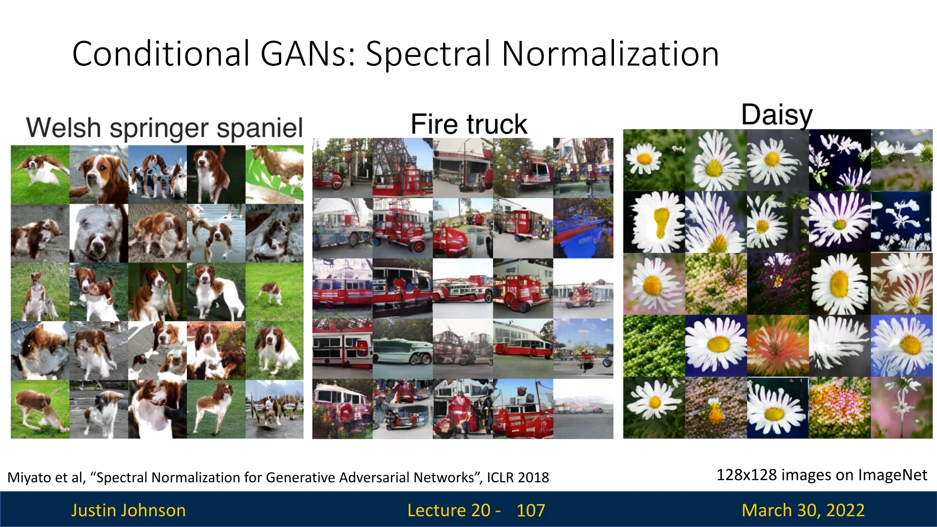
Alternative Loss: Hinge Loss Formulation While the non-saturating GAN loss is commonly used in conditional GANs with CBN, another widely adopted objective—especially in more recent setups such as this work and BigGANs—is the hinge loss we’ve covered previously with SVMs §3.6.4. It replaces the cross-entropy terms with a margin-based objective, helping the discriminator focus on classification margins and improving gradient stability.
Hinge loss (for conditional GANs) \[ \begin {aligned} \mathcal {L}_D &= \mathbb {E}_{x \sim p_{\mbox{data}}} \left [ \max (0, 1 - D(x, y)) \right ] + \mathbb {E}_{z \sim p(z)} \left [ \max (0, 1 + D(G(z, y), y)) \right ] \\ \mathcal {L}_G &= - \mathbb {E}_{z \sim p(z)} \left [ D(G(z, y), y) \right ] \end {aligned} \]
Intuition:
- The discriminator learns to assign a positive score (ideally \(\geq 1\)) to real images \((x, y)\), and a negative score (ideally \(\leq -1\)) to generated images \(G(z, y)\).
- If a sample is already on the correct side of the margin (e.g., a real image with \(D(x, y) > 1\)), the loss is zero — no gradient is applied.
- The generator is trained to maximize the discriminator’s score for its outputs (i.e., make fake images look real to the discriminator).
Why hinge loss helps
- Avoids vanishing gradients when the discriminator becomes too confident (a problem with \(-\log (1 - D(G(z)))\) in early GANs).
- Simplifies optimization with piecewise-linear objectives.
- Empirically improves convergence speed and stability, particularly when combined with spectral normalization.
- Stable Training: With a 1-Lipschitz constraint, the discriminator avoids extreme gradients; the generator receives more reliable updates.
- No Extra Gradient Penalties: Unlike methods (e.g., WGAN-GP) that add penalty terms, SN modifies weights directly, incurring lower overhead.
- Enhanced Diversity: By preventing the discriminator from collapsing too fast, SN often yields more diverse generated samples and mitigates mode collapse.
In practice, Spectral Normalization integrates neatly with standard deep learning frameworks, requiring minimal changes to existing layers. It has become a mainstay technique for reliably training high-quality GANs, used in both unconditional and conditional setups.
Enrichment 20.7.3: Self-Attention GANs (SAGAN)
While convolutional GANs operate effectively on local patterns, they struggle with modeling long-range dependencies, especially in complex scenes. In standard convolutions, each output pixel is influenced only by a small neighborhood of input pixels, and even deep networks require many layers to connect distant features. This becomes problematic in global structure modeling — e.g., maintaining symmetry across a face or coherence across distant body parts.
Self-Attention GANs (SAGAN) [784] address this limitation by integrating non-local self-attention layers into both the generator and discriminator. This allows the model to reason about all spatial locations simultaneously, capturing long-range dependencies without requiring deep, inefficient convolutional hierarchies.
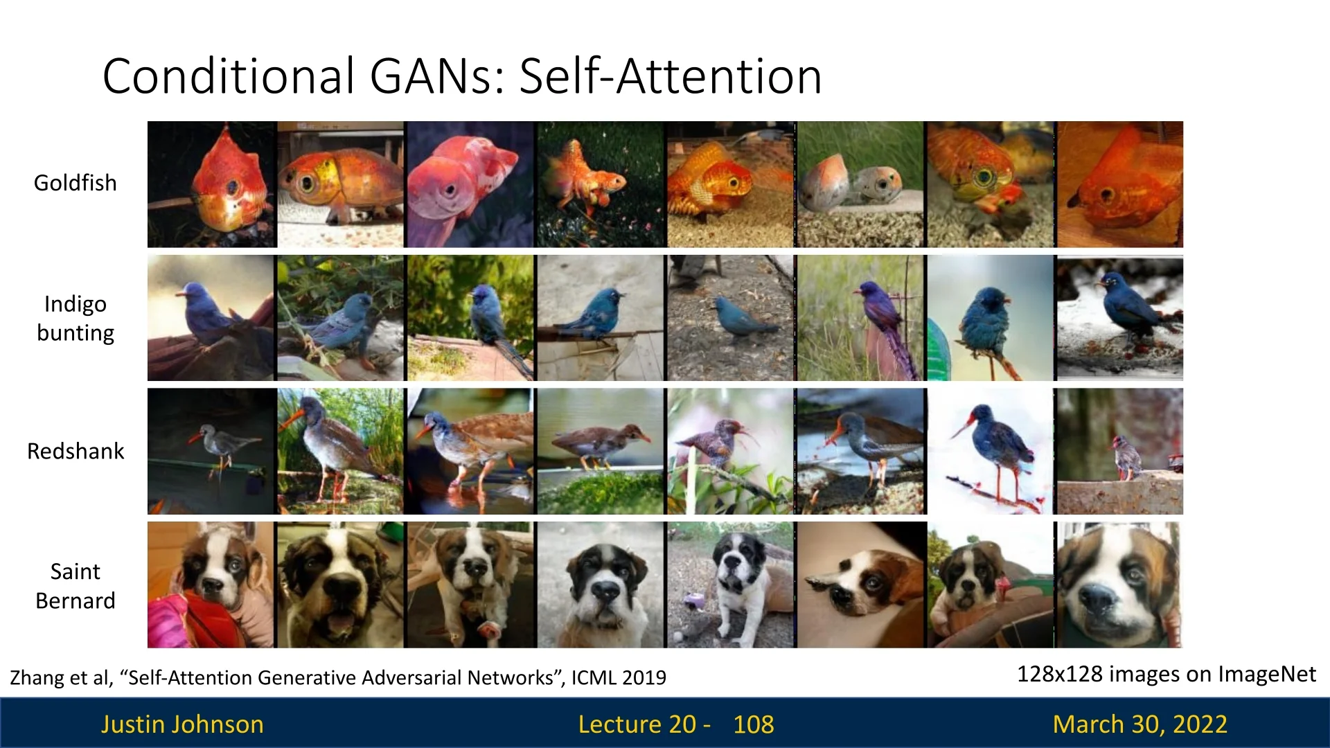
Architecture Overview The self-attention block follows the ”query–key–value” formulation:
- Given an input feature map \( X \in \mathbb {R}^{C \times H \times W} \), three \( 1 \times 1 \) convolutions produce: \( f(X) \) (queries), \( g(X) \) (keys), and \( h(X) \) (values).
- Queries and keys are reshaped to \( C' \times N \) (with \( N = H \cdot W \)) and multiplied, yielding a \( N \times N \) attention map.
- A softmax ensures attention scores sum to 1 across each row (normalized over keys).
- The result is multiplied with values \( h(X) \) and reshaped back to the spatial layout.
- A learnable scale parameter \( \gamma \), initialized to zero, controls the strength of the attention output: \( \mbox{Output} = \gamma \cdot \mbox{SelfAttention}(X) + X \).
- Facilitates global reasoning — e.g., the left eye can align symmetrically with the right, even if they are spatially far apart.
- Improves texture consistency and fine-grained detail preservation in images.
- Enhances expressiveness in multi-class generation tasks like ImageNet.
Training Details and Stabilization SAGAN adopts two key techniques for stable training:
- 1.
- Spectral Normalization [451] applied to both generator and discriminator (unlike earlier approaches which only normalized the discriminator). This constrains each layer’s Lipschitz constant, preventing exploding gradients and improving convergence.
- 2.
- Two Time-Scale Update Rule (TTUR): The generator and discriminator are updated with separate learning rates. This allows the discriminator to stabilize quickly while the generator catches up.
Their combination leads to faster convergence, improved stability, and better FID/IS scores.
Loss Function SAGAN uses the hinge version of the adversarial loss: \[ \mathcal {L}_D = \mathbb {E}_{x \sim p_{\mbox{data}}}[\max (0, 1 - D(x))] + \mathbb {E}_{z \sim p(z)}[\max (0, 1 + D(G(z)))] \] \[ \mathcal {L}_G = - \mathbb {E}_{z \sim p(z)}[D(G(z))] \] This formulation improves gradient behavior by clearly separating the penalties for incorrect real/fake classification.
Quantitative Results SAGAN significantly improves generative performance:
- Achieves state-of-the-art FID and IS scores on ImageNet (128×128).
- Produces semantically consistent outputs, outperforming convolution-only GANs especially on complex classes like “dog” or “person”.
Summary Self-attention enables the generator and discriminator to capture global structures efficiently, helping GANs go beyond local textures. This innovation inspired later models like BigGAN [52], which combine attention, large-scale training, and class conditioning to achieve unprecedented photorealism.
Enrichment 20.7.4: BigGANs: Scaling Up GANs
BigGAN [52] marks a major milestone in the progression of class-conditional GANs by demonstrating that simply scaling up the model and training setup—when coupled with key stabilization techniques—yields state-of-the-art performance across resolution, sample fidelity, and class diversity. Developed by Brock et al., BigGAN pushes the frontier of GAN-based image synthesis, particularly on challenging datasets like ImageNet and JFT-300M.
Key Innovations and Techniques
- Conditional Batch Normalization (CBN): Class labels are incorporated deep into the generator via Conditional BatchNorm layers. Each BatchNorm is modulated by gain and bias vectors derived from a shared class embedding, enabling class-conditional feature modulation.
- Projection-Based Discriminator: The discriminator uses projection [451] to incorporate class information, effectively learning to assess whether an image is both real and aligned with its target class.
- Spectral Normalization (SN): Applied to both \( G \) and \( D \), SN constrains the Lipschitz constant of each layer, enhancing training stability by regularizing weight scales.
- Large-Scale Batch Training: Batch sizes as large as 2048 are used, significantly improving gradient quality and enabling more stable optimization trajectories. Larger batches cover more modes and support smoother convergence.
- Skip-\( z \) Connections: Latent vectors are not only injected at the generator input but also directly routed to multiple residual blocks at various resolutions. These skip connections facilitate hierarchical control over spatial features.
- Residual Architecture: Deep residual blocks enhance gradient flow and feature reuse. BigGAN-deep further expands the architecture using bottleneck ResBlocks and additional layers per resolution.
- Orthogonal Regularization: To support the truncation trick, orthogonal regularization [55] ensures the generator’s mapping from latent space is smooth and well-conditioned. This regularization minimizes cosine similarity between filters while avoiding norm constraints.
- Truncation Trick: During inference, samples are drawn from a truncated normal distribution, i.e., \( z \sim \mathcal {N}(0, I) \) with resampling of values exceeding a fixed magnitude threshold. This concentrates latent inputs around the distribution’s mode, improving visual fidelity at the cost of diversity. The truncation threshold serves as a dial for post-hoc control over the quality–variety tradeoff.
- Exponential Moving Average (EMA): The generator weights are averaged across training steps using an EMA with a decay of 0.9999, improving the quality and consistency of generated samples during evaluation.
- Orthogonal Initialization: All layers in \( G \) and \( D \) are initialized with orthogonal matrices [570], promoting stable signal propagation in very deep networks.
- Hinge Loss and Self-Attention: The architecture adopts hinge loss for adversarial training and includes self-attention modules [784] to improve long-range dependency modeling, especially in higher-resolution images.
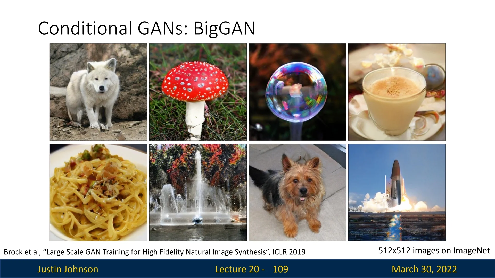
Beyond the primary components discussed in earlier parts of this lecture such as label conditioning, spectral normalization, and self-attention—BigGAN incorporates several additional architectural and training innovations that play a crucial role in achieving high-fidelity, scalable synthesis. In what follows, we elaborate on these techniques, mainly those which were not previously covered in depth.
Enrichment 20.7.4.1: Skip-\( z \) Connections: Hierarchical Latent Injection
In conventional conditional GANs, the latent code \( z \in \mathbb {R}^{d} \) is typically introduced at the generator’s input layer and optionally used to initialize class-conditional batch normalization (CBN) in a uniform way. However, this limits the model’s ability to control spatially localized features in a deep generator architecture.
BigGAN implements a refined variant of latent conditioning, referred to as skip-\( z \) connections. The latent vector \( z \) is evenly split into \( L \) chunks—each assigned to one of the generator’s \( L \) residual blocks. Each block uses its assigned chunk \( z_\ell \in \mathbb {R}^{d/L} \) in combination with the shared class embedding \( c \in \mathbb {R}^{d_c} \) to compute block-specific conditional normalization parameters.
- 1.
- Concatenate \( z_\ell \) with \( c \).
- 2.
- Project this vector using two linear layers to produce the gain and bias for CBN.
- 3.
- Apply those to modulate the BatchNorm activations within the residual block.
This process occurs twice per block (once for each BatchNorm layer), and is implemented via reusable layers inside each residual block.
# From BigGAN-PyTorch: ConditionalBatchNorm2d
class ConditionalBatchNorm2d(nn.Module):
def __init__(self, num_features, cond_dim):


super().__init__()
self.bn = nn.BatchNorm2d(num_features, affine=False)
self.gain = nn.Linear(cond_dim, num_features)
self.bias = nn.Linear(cond_dim, num_features)


def forward(self, x, y):  # y = [z_chunk, class_embedding]


out = self.bn(x)
gamma = self.gain(y).unsqueeze(2).unsqueeze(3)
beta = self.bias(y).unsqueeze(2).unsqueeze(3)
return gamma * out + beta
Each residual block in the generator stores its own ‘ConditionalBatchNorm2d‘ instances and receives its dedicated chunk of \( z \). This allows each layer to capture different aspects of semantic control—for example, coarse structures at lower resolution, textures and edges at higher ones.
Comparison to Standard CBN: In standard conditional normalization, the generator is conditioned on a single global class embedding \( c \), which is reused across all layers. This provides semantic conditioning but lacks spatial specificity. In BigGAN, the class embedding \( c \) remains global and shared, but the latent vector \( z \) is partitioned into chunks \( z^{(l)} \), one per generator block. Each chunk influences a different spatial resolution by being fed into that block’s conditional batch normalization (CBN) layer.
This design allows different parts of the latent code to control different levels of the image hierarchy — from coarse global structure to fine-grained texture. As a result, the generator gains more expressive power and learns a hierarchical organization of semantic and stylistic attributes without modifying the way \( c \) is handled.
BigGAN-deep Simplification: In BigGAN-deep, the latent vector \( z \) is not split. Instead, the full \( z \) vector is concatenated with the class embedding and injected identically into every residual block. While this sacrifices per-layer specialization of \( z \), it simplifies parameter management and works effectively in deeper, bottlenecked architectures.
Enrichment 20.7.4.2: Residual Architecture: Deep and Stable Generators
A cornerstone of BigGAN’s scalability is its reliance on deep residual networks in both the generator and discriminator. Inspired by ResNet-style design [215], BigGAN structures its generator using stacked residual blocks, each of which learns a refinement over its input, enabling stable and expressive function approximation even at hundreds of layers.
Motivation and Design: GAN training becomes increasingly unstable as model capacity grows. Residual blocks counteract this by providing shortcut (identity) connections that facilitate gradient propagation and feature reuse. Each residual block contains:
- Two \( 3 \times 3 \) convolutions (optionally bottlenecked).
- Two conditional batch normalization layers (CBN), conditioned via skip-\( z \) as described earlier.
- A ReLU activation before each convolution.
- A learned skip connection (via \(1\times 1\) conv) when input/output shapes differ.
This design supports deep, expressive generators that do not suffer from vanishing gradients.
BigGAN vs. BigGAN-deep: BigGAN uses relatively shallow residual blocks with a single block per resolution stage. In contrast, BigGAN-deep significantly increases network depth by introducing:
- Two residual blocks per resolution (instead of one).
- Bottlenecked residual layers: each block includes \(1 \times 1\) convolutions before and after the main \(3 \times 3\) convolution to reduce and restore the channel dimensionality.
- Identity-preserving skip connections: in the generator, excess channels are dropped to match dimensions, while in the discriminator, missing channels are padded via concatenation.
These architectural changes enable deeper networks with better training stability and more efficient parameter usage.
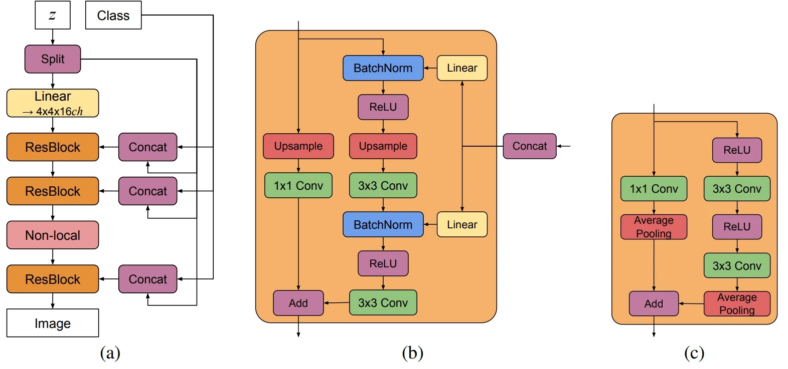
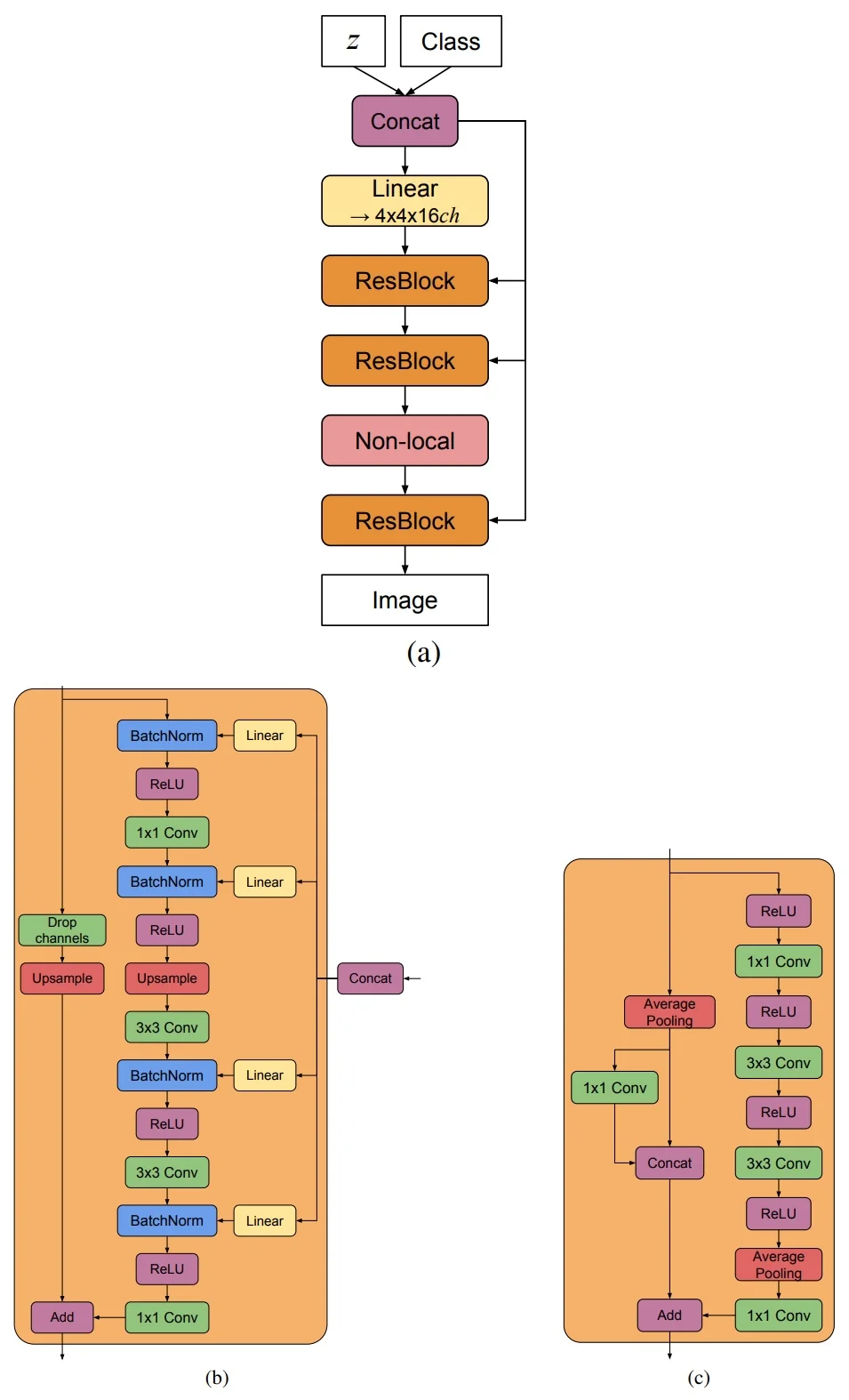
These deeper and more modular residual structures help BigGAN-deep outperform its shallower predecessor across all resolutions and evaluation metrics (e.g., FID and IS), while often using fewer parameters due to the bottlenecked design.
Enrichment 20.7.4.3: Truncation Trick in BigGAN: Quality vs. Diversity
The truncation trick is a sampling technique introduced in BigGAN [52] to improve image quality during inference. It restricts latent vectors to lie within a high-density region of the standard normal distribution, where the generator is more likely to produce stable and realistic outputs.
Truncated Normal Distributions in Latent Space During training, the latent code \( z \in \mathbb {R}^d \) is drawn from a standard normal distribution, \( z_i \sim \mathcal {N}(0, 1) \). At test time, the truncation trick samples each component from the same distribution but only accepts values within an interval \( [-\tau , \tau ] \). Formally: \[ z_i \sim \mathcal {N}(0, 1) \quad \mbox{conditioned on} \quad |z_i| \leq \tau \] Samples exceeding \( \tau \) are rejected and resampled. This results in a truncated normal distribution with increased density near the origin and zero probability beyond the cutoff. The distribution is renormalized so that it still integrates to 1.
Why Truncate? In high-dimensional Gaussian space, most probability mass is concentrated in a thin spherical shell around \( \|z\|_2 \approx \sqrt {d} \). These high-norm vectors are often mapped by the generator to unstable or low-quality outputs. Truncation focuses sampling on lower-norm vectors near the origin—regions where the generator has been well-trained. This leads to:
- Cleaner and sharper images.
- Reduced artifacts.
- Stronger alignment with class-conditional structure.
How Is \( \tau \) Chosen? The truncation threshold \( \tau \) is a tunable hyperparameter. Smaller values yield higher quality but reduce diversity. Common values include \( \tau = 2.0 \), \( 1.5 \), \( 1.0 \), or \( 0.5 \). In practice, a truncation sweep is performed to empirically select the best trade-off. BigGAN reports IS and FID for multiple truncation levels, revealing the tradeoff curve between sample quality and variety.
Implementation in Practice Truncated sampling is implemented via per-dimension rejection sampling:
from scipy.stats import truncnorm


def truncated_z(dim, tau):


return truncnorm.rvs(-tau, tau, loc=0, scale=1, size=dim)
This procedure generates a latent vector \( z \in \mathbb {R}^d \) with each component sampled independently from \( \mathcal {N}(0, 1) \), truncated to \( [-\tau , \tau ] \).
Tradeoffs and Limitations Truncation improves sample fidelity but comes with costs:
- Reduced Diversity: A smaller volume of latent space is explored.
- Possible Instability: Generators not trained to handle low-norm regions may produce collapsed or saturated outputs.
When Truncation Fails If the generator lacks smoothness near \( z = 0 \), truncation can trigger saturation artifacts or mode collapse. This happens when the model overfits to high-norm training inputs and generalizes poorly to low-norm regions. Thus, truncation should be used only with generators that have been explicitly regularized for this purpose.
How to Make Truncation Work Reliably To ensure that the generator behaves well under truncation, BigGAN applies orthogonal regularization, which promotes smoothness and local isometry in the latent-to-image mapping. This regularization term discourages filter redundancy and ensures the generator responds predictably to small latent variations—especially those near the origin.
Enrichment 20.7.4.4: Orthogonal Regularization: A Smoothness Prior for Truncated Latents
Orthogonal regularization is a key technique introduced in BigGAN to ensure that the generator remains well-behaved in low-norm regions of latent space—regions emphasized by the truncation trick. While truncation improves sample quality by concentrating latent inputs near the origin, this strategy only works reliably if the generator maps these inputs smoothly and predictably to images. Without this property, truncation may lead to artifacts, over-saturation, or even complete mode collapse.
To address this, BigGAN introduces a soft form of orthogonality constraint on the generator’s weight matrices. The goal is to encourage the columns of each weight matrix to be approximately orthogonal to each other. This makes each layer in the generator act as a near-isometric transformation, where similar inputs lead to similar outputs. As a result, local neighborhoods in latent space map to locally coherent image regions.
The standard orthogonal regularization term penalizes deviations from strict orthogonality by minimizing the squared Frobenius norm of the off-diagonal entries in \( W^\top W \), where \( W \) is a weight matrix: \[ \mathcal {L}_{\mbox{ortho}} = \lambda \left \| W^\top W - I \right \|_F^2 \] However, in practice, this constraint is too strong and can limit model expressiveness. Instead, BigGAN uses a relaxed variant that excludes the diagonal entries, focusing only on reducing correlations between filters while allowing their norms to vary. The regularization term becomes: \[ \mathcal {L}_{\mbox{ortho}} = \lambda \left \| W^\top W \odot (1 - I) \right \|_F^2 \] where \( I \) is the identity matrix and \( \odot \) denotes element-wise multiplication. This version of the penalty preserves the desired smoothness properties without overly constraining the generator’s capacity.
Empirical results show that orthogonal regularization dramatically increases the likelihood that a generator will remain stable under truncated sampling. In the BigGAN paper, only 16% of large models were truncation-tolerant without orthogonal regularization.
When this penalty was included, the success rate increased to over 60%. These results confirm that enforcing orthogonality improves the conditioning of the generator and mitigates gradient pathologies that would otherwise arise in narrow latent regions.
In implementation, orthogonal regularization is applied as an auxiliary term added to the generator’s loss during training. It is computed across all linear and convolutional weight matrices using simple matrix operations. Its computational overhead is negligible compared to the benefits it provides in stability, generalization, and quality at inference time—particularly when truncated latent vectors are used.
Orthogonal regularization should not be confused with orthogonal initialization, although both arise from the same geometric motivation: preserving distance and structure through linear transformations. Orthogonal initialization sets the initial weights of a neural network to be orthogonal matrices, satisfying \( W^\top W = I \) at initialization time. This technique was introduced in the context of deep linear and recurrent networks [570] to maintain variance propagation and avoid gradient explosion or vanishing.
BigGAN applies orthogonal initialization to all convolutional and linear layers in both the generator and the discriminator. This initialization ensures that the model starts in a well-conditioned regime where activations and gradients are stable across many layers. However, during training, weight matrices are updated by gradient descent and quickly deviate from orthogonality. This is where orthogonal regularization becomes essential—it continuously nudges the model back toward this structured regime.
Thus, orthogonal initialization provides a favorable starting point, while orthogonal regularization acts as a guiding prior during optimization. Their combination is especially effective in large-scale GANs: initialization alone may be insufficient to prevent pathological gradients, and regularization alone may be ineffective if starting from arbitrary weights. Together, they enable BigGAN to maintain spatial smoothness and local isometry throughout training, which is critical for its ability to support low-norm latent vectors and reliably generate high-quality images under truncation.
Enrichment 20.7.4.5: Exponential Moving Average (EMA) of Generator Weights
Another subtle but powerful technique used in BigGAN is the application of an exponential moving average (EMA) over the generator weights during training. Although it does not influence the optimization process directly, EMA plays a critical role during evaluation and sample generation. It acts as a temporal smoothing mechanism over the generator’s parameter trajectory, helping to counteract the noise and instability of high-variance gradient updates that occur throughout adversarial training.
The EMA maintains a running average of the generator’s weights \( \theta _t \) according to the update rule: \[ \theta ^{\mbox{EMA}}_t = \alpha \cdot \theta ^{\mbox{EMA}}_{t-1} + (1 - \alpha ) \cdot \theta _t \] where \( \alpha \in (0, 1) \) is the decay rate, often set very close to 1 (e.g., \( \alpha = 0.999 \) or \( 0.9999 \)). This formulation gives exponentially more weight to recent updates while slowly fading out older values. As training progresses, the EMA model tracks the moving average of each parameter across steps, effectively producing a smoothed version of the generator that is less affected by momentary oscillations or adversarial instability.
In practice, EMA is not used during training updates or backpropagation. Instead, a shadow copy of the generator is maintained and updated using the EMA formula after each optimization step.
Then, when it comes time to evaluate the generator—either for computing metrics like Inception Score or FID, or for sampling images for qualitative inspection—BigGAN uses this EMA-smoothed generator instead of the raw, most-recent checkpoint.
The benefits of this approach are particularly visible in high-resolution settings, where adversarial training can produce noisy or unstable weight fluctuations even when the model as a whole is converging. The EMA model filters out these fluctuations, resulting in visibly cleaner and more coherent outputs. It also improves quantitative metrics across the board, with lower FID scores and reduced sample variance across random seeds.
The idea of averaging model parameters over time is not unique to GANs—it has a long history in convex optimization and stochastic learning theory, and is closely related to Polyak averaging. However, in the context of GANs, it gains particular significance due to the non-stationary nature of the loss surface and the adversarial updates. The generator is not optimizing a static objective but is instead constantly adapting to a co-evolving discriminator. EMA helps decouple the generator from this shifting target by producing a more stable parameter estimate over time.
It is also worth noting that EMA becomes increasingly important as model size and capacity grow. In very large generators, even small perturbations to weight matrices can lead to visible differences in output. This sensitivity is amplified when using techniques like truncation sampling, which further constrain the input space. The EMA generator mitigates these issues by producing a version of the model that is representative of the broader training trajectory, rather than any single volatile moment in optimization.
In BigGAN, the EMA weights are typically stored alongside the training weights, and a final evaluation pass is conducted exclusively using the averaged version. This ensures that reported metrics reflect the most stable version of the model. As a result, EMA has become a de facto standard in high-quality GAN implementations, extending well beyond BigGAN into diffusion models, VAEs, and other generative frameworks that benefit from stable parameter averaging.
Enrichment 20.7.4.6: Discriminator-to-Generator Update Ratio
A key practical detail in BigGAN’s training strategy is its use of an asymmetric update schedule between the generator and discriminator. Specifically, for every generator update, the discriminator is updated twice. This 2:1 update ratio, while simple, has a significant impact on training stability and convergence—particularly during early stages when the generator is still producing low-quality outputs and lacks meaningful gradients.
This design choice arises from the fundamental nature of GANs as a two-player minimax game rather than a supervised learning problem. In the standard GAN objective, the generator relies on the discriminator to provide gradients that guide it toward producing more realistic samples. If the discriminator is undertrained or inaccurate, it fails to deliver informative gradients. In such cases, the generator may either receive gradients with very low magnitude (i.e., saturated) or gradients that are inconsistent and directionless. Either scenario leads to unstable training, poor convergence, or mode collapse.
Updating the discriminator more frequently ensures that it can closely track the current distribution of fake samples produced by the generator. In early training, this is especially important: the generator often outputs near-random images, while the discriminator can quickly learn to distinguish these from real samples. However, the generator can only learn effectively if the discriminator provides non-saturated gradients—responses that are confident yet not flat. By giving the discriminator extra updates, the model maintains a discriminator that is sufficiently strong to provide meaningful feedback but not so dominant that it collapses the generator.
This update schedule also compensates for the relatively high gradient variance and weaker signal that the generator typically receives. Since the generator’s loss depends entirely on how the discriminator scores its outputs, and because these outputs change with each batch, the gradient landscape faced by the generator is inherently less stable. Additional discriminator updates help mitigate this instability by ensuring that the discriminator has time to adapt to the generator’s latest distribution before a new generator step is taken.
Importantly, this strategy only works in combination with proper regularization. BigGAN uses spectral normalization in both \( G \) and \( D \) to constrain the discriminator’s Lipschitz constant and prevent overfitting. Without such constraints, training the discriminator more aggressively could lead it to perfectly memorize the training data or overpower the generator entirely, resulting in vanishing gradients.
While BigGAN settles on a 2:1 update ratio, other GAN variants may use different values depending on model complexity and the chosen loss function. For example, WGAN-GP updates the discriminator five times for every generator update to approximate the Wasserstein distance reliably. In contrast, StyleGAN2-ADA uses a 1:1 schedule but includes strong regularization and adaptive data augmentation to stabilize training. Ultimately, the ideal update frequency is a function of architectural depth, dataset difficulty, and the adversarial loss landscape. In BigGAN’s case, the 2:1 ratio is a well-calibrated compromise that supports rapid discriminator adaptation without overwhelming the generator.
Results and Legacy Trained on ImageNet, BigGAN models achieved an Inception Score (IS) of 166.5 and FID of 7.4 at \(128\times 128\) resolution—substantially surpassing previous benchmarks. The models generalize well to larger datasets such as JFT-300M and have inspired a cascade of follow-up works, including:
- BigBiGAN [132], which extends BigGAN with an encoder network, enabling bidirectional mapping and representation learning;
- ADM-G [124], whose strong results in class-conditional image synthesis with diffusion models were, in part, motivated by BigGAN’s performance ceiling;
- StyleGAN-T [569], a transformer-based GAN combining BigGAN-style residual backbones with Vision Transformer decoders;
- Consistency Models [602], which revisit training efficiency, stability, and realism tradeoffs using simplified objectives beyond GANs.
These extensions signal BigGAN’s long-standing impact—not merely as a powerful model, but as a catalyst for the generative modeling community’s move toward scalable, stable, and controllable synthesis. Its emphasis on architectural regularization, batch scaling, and sample quality–diversity tradeoffs continues to shape SOTA pipelines.
Enrichment 20.7.5: StackGAN: Two-Stage Text-to-Image Synthesis
StackGAN [785] introduced a pivotal advancement in text-to-image generation by proposing a two-stage architecture that decomposes the synthesis process into coarse sketching and progressive refinement. This design is inspired by how human artists typically work: first sketching global structure, then layering fine-grained detail. The central insight is that generating high-resolution, photorealistic images directly from text is extremely difficult—both because modeling fine detail in a single forward pass is computationally unstable, and because the generator must preserve semantic alignment with the conditioning text at increasing resolutions.
Earlier works such as GAN-INT-CLS [535] and GAWWN [536] introduced conditional GANs based on text embeddings. GAN-INT-CLS used a pre-trained RNN to encode descriptive captions into fixed-size vectors, which were then concatenated with noise and passed through a generator to produce \(64 \times 64\) images. While conceptually sound, it failed to capture high-frequency details or generate sharp textures. GAWWN added spatial attention and object location hints, but similarly struggled at scaling beyond low resolutions or preserving semantic richness.
StackGAN addresses these challenges by introducing a two-stage generator pipeline. But before either stage operates, StackGAN applies a crucial transformation called Conditioning Augmentation (CA). Instead of feeding the text embedding \( \phi _t \in \mathbb {R}^D \) directly into the generator, CA maps it to a Gaussian distribution \( \mathcal {N}(\mu (\phi _t), \Sigma (\phi _t)) \) using a learned mean and diagonal covariance. A conditioning vector \( \hat {c} \sim \mathcal {N}(\mu , \Sigma ) \) is then sampled and used as the actual conditioning input.
This stochastic perturbation serves several purposes:
- It encourages smoothness in the conditioning manifold, making the generator less brittle to small changes in text.
- It introduces variation during training, acting like a regularizer that improves generalization.
- It helps overcome mode collapse by encouraging the generator to explore nearby conditioning space without drifting far from the intended semantics.
With CA in place, StackGAN proceeds in two stages:
- Stage-I Generator: Takes as input the sampled conditioning vector \( \hat {c} \) and a random noise vector \( z \), and synthesizes a coarse \(64 \times 64\) image. This image captures the global layout, color palette, and rough object geometry implied by the text. However, it typically lacks sharpness and fine-grained texture.
- Stage-II Generator: Refines the low-resolution image by conditioning again on the original text embedding (not the sampled \( \hat {c} \)) and the Stage-I output. It corrects distortions, enhances object boundaries, and synthesizes photorealistic detail. This generator is built as a residual encoder–decoder network, with upsampling layers and deep residual connections that allow semantic feature reuse. The discriminator in this stage is also enhanced with matching-aware supervision to ensure image–text consistency.
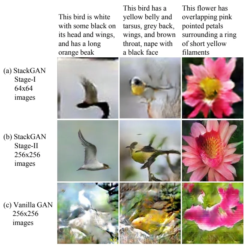
The effect of this staged generation is illustrated in Figure 20.45. While one-stage GANs struggle to produce realistic \(256 \times 256\) images—even when equipped with deep upsampling layers—StackGAN’s sketch-and-refine paradigm achieves significantly better visual fidelity. Stage-I outputs provide rough structure, and Stage-II convincingly improves resolution, texture, and alignment with text cues.
The architectural overview illustrates the interaction between text embeddings, conditioning augmentation, and residual refinement. The text embedding is used at both stages to ensure that conditioning information is not lost in early transformations. Residual blocks in Stage-II integrate features from both the coarse image and the original text to construct plausible details aligned with the semantics of the prompt.
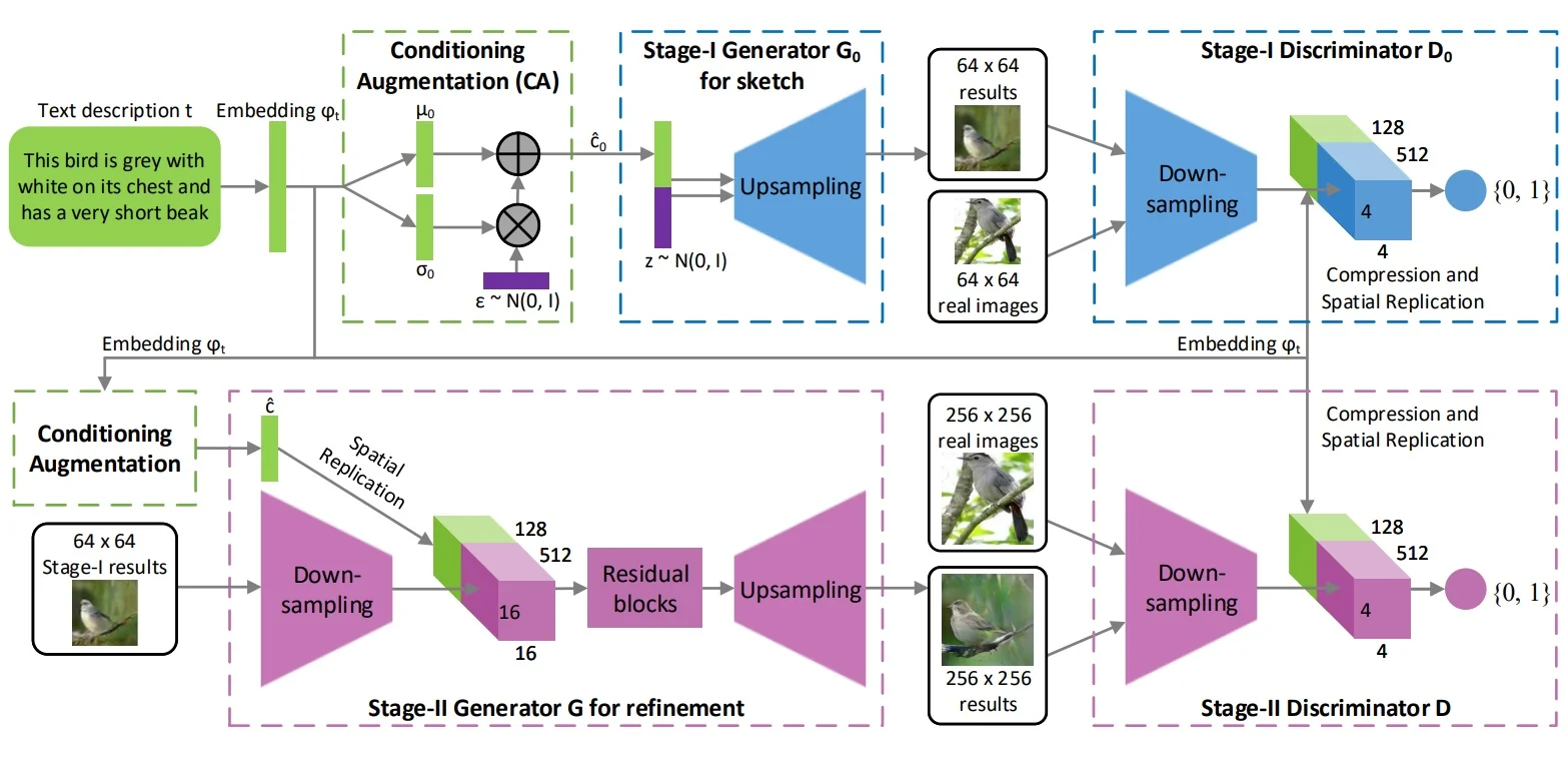
This two-stage framework offers several advantages:
- It decomposes the generation task into manageable subgoals: layout and detail.
- It maintains semantic consistency by conditioning both stages on the text.
- It improves training stability and image diversity through CA.
From Overview to Components: We now examine each of StackGAN’s core components in detail. The entire system is built on a simple but powerful idea: rather than attempting to generate high-resolution images in a single step, StackGAN decomposes the process into well-defined stages. Each stage plays a specialized role in the pipeline, and the quality of the final output hinges critically on the strength of the conditioning mechanism that feeds it.
We begin by studying Conditioning Augmentation (CA), which precedes both Stage-I and Stage-II generators and provides the stochastic conditioning vector from which the entire synthesis process unfolds. This module acts as the semantic foundation of StackGAN, and understanding it will clarify how subsequent stages achieve stability, diversity, and realism.
Enrichment 20.7.5.1: Conditioning Augmentation (CA)
A central challenge in text-conditioned GANs is that each natural language caption is mapped to a fixed high-dimensional embedding vector \( \phi _t \in \mathbb {R}^D \), typically obtained via an RNN-based text encoder. While these embeddings successfully encode semantics, they pose three major problems for image generation:
- Determinism: A single text embedding maps to a single point in feature space, limiting image diversity for the same caption.
- Sparsity and Interpolation Gaps: Fixed embeddings lie on a sparse, irregular manifold, making interpolation and smooth generalization difficult.
- Overfitting: The generator may memorize how to map a specific caption embedding to a specific image, risking mode collapse.
Solution: Learn a Distribution Over Conditioning Vectors StackGAN addresses these issues with Conditioning Augmentation (CA), which models a distribution over conditioning vectors rather than using a single deterministic embedding. Given a text embedding \( \phi _t \), CA learns the parameters of a Gaussian distribution: \[ \hat {c} \sim \mathcal {N}\left ( \mu (\phi _t), \operatorname {diag}(\sigma ^2(\phi _t)) \right ) \] where \( \mu (\phi _t) \in \mathbb {R}^{N_g} \) and \( \log \sigma ^2(\phi _t) \in \mathbb {R}^{N_g} \) are the outputs of two fully connected layers applied to \( \phi _t \). This distribution introduces controlled randomness into the conditioning process.
Sampling via Reparameterization Trick To ensure end-to-end differentiability, CA uses the reparameterization trick—first introduced in variational autoencoders: \[ \hat {c} = \mu (\phi _t) + \sigma (\phi _t) \odot \epsilon , \qquad \epsilon \sim \mathcal {N}(0, I) \] where \( \hat {c} \in \mathbb {R}^{N_g} \) becomes the actual conditioning input for the generator, and \( \odot \) denotes elementwise multiplication. This trick enables gradients to propagate through the stochastic sampling process during training.
KL Divergence Regularization To avoid arbitrary shifts in the learned distribution and ensure it remains centered and stable, CA includes a regularization term: \[ \mathcal {L}_{\mathrm {KL}} = D_{\mathrm {KL}}\left ( \mathcal {N}(\mu (\phi _t), \operatorname {diag}(\sigma ^2(\phi _t))) \;\|\; \mathcal {N}(0, I) \right ) \] This KL divergence penalizes deviations from the standard normal distribution, thereby encouraging the learned \( \mu \) to stay near zero and \( \sigma \) near one. This regularization discourages degenerate behavior such as collapsing the variance to zero (making CA deterministic again). The KL loss is added to the generator’s total loss during training.
Benefits of Conditioning Augmentation
- Diversity from Fixed Input: Sampling \( \hat {c} \) from a learned Gaussian allows multiple plausible images to be generated from a single caption \( \phi _t \).
- Smooth Latent Manifold: The conditioning space becomes more continuous, improving interpolation, generalization, and gradient flow.
- Robustness and Regularization: The KL penalty prevents the conditioning distribution from drifting arbitrarily far from the origin, which stabilizes training.
Summary Table: Conditioning Augmentation
| Component | Role |
|---|---|
| \( \phi _t \) | Sentence embedding from text encoder |
| \( \mu (\phi _t), \sigma ^2(\phi _t) \) | Parameters of a diagonal Gaussian |
| \( \hat {c} \) | Sampled conditioning vector fed to the generator |
| \( \mathcal {L}_{\mathrm {KL}} \) | Regularizer to keep \( \mathcal {N}(\mu , \sigma ^2) \) close to \( \mathcal {N}(0, I) \) |
Having established a robust and diverse conditioning vector \( \hat {c} \) via CA, we now turn to the first stage of generation: a low-resolution GAN that translates this semantic vector into a coarse but globally coherent image layout.
Enrichment 20.7.5.2: Stage-I Generator: Coarse Sketching from Noise and Caption
After sampling a stochastic conditioning vector \( \hat {c} \in \mathbb {R}^{N_g} \) via Conditioning Augmentation (CA), the Stage-I generator synthesizes a coarse \( 64 \times 64 \) image that captures the global layout, dominant colors, and rough object shapes. This stage is intentionally lightweight, focusing not on photorealism, but on producing a semantically plausible sketch aligned with the text description.
Motivation: Why Two Stages? Generating high-resolution images (e.g., \(256 \times 256\)) directly from noise and text is challenging due to multiple factors:
- Gradient instability: GAN training at large resolutions often suffers from unstable optimization.
- Complex mappings: A direct mapping from \( (z, \phi _t) \mapsto \mbox{image} \) must simultaneously learn global structure and fine-grained detail.
- Mode collapse: High-resolution generation without strong inductive structure can lead to poor sample diversity or overfitting.
To mitigate these issues, StackGAN breaks the synthesis process into two distinct tasks:
- Stage-I: Learn to generate a coarse image from the conditioning vector.
- Stage-II: Refine that image into a high-fidelity result using residual enhancement.
This decomposition improves modularity, training stability, and sample quality, following the same coarse-to-fine approach used in human drawing.
Architecture of Stage-I Generator The generator takes as input: \[ z \sim \mathcal {N}(0, I), \qquad \hat {c} \sim \mathcal {N}(\mu (\phi _t), \sigma ^2(\phi _t)) \] where \( z \in \mathbb {R}^{N_z} \) is a standard Gaussian noise vector and \( \hat {c} \in \mathbb {R}^{N_g} \) is the sampled conditioning vector. These vectors are concatenated to form a combined input: \[ h_0 = [z; \hat {c}] \in \mathbb {R}^{N_z + N_g} \]
The forward pass proceeds as follows:
- 1.
- Fully connected layer: \( h_0 \) is mapped to a dense feature vector and reshaped to a spatial tensor (e.g., \( 4 \times 4 \times 512 \)).
- 2.
- Upsampling blocks: A series of convolutional blocks upsample this tensor
progressively to \(64 \times 64\), each consisting of:
- Nearest-neighbor upsampling (scale factor 2)
- \(3 \times 3\) convolution to reduce channel dimensionality
- Batch Normalization
- ReLU activation
- 3.
- Final layer: A \(3 \times 3\) convolution maps the output to 3 channels (RGB), followed by a Tanh activation: \[ I_{\mbox{stage-I}} = \tanh (\mbox{Conv}_{\mbox{RGB}}(h)) \in \mathbb {R}^{64 \times 64 \times 3} \]
Output Normalization: Why Tanh? The Tanh function ensures that pixel values lie in the range \( (-1, 1) \). This matches the normalized data distribution used during training and avoids vanishing gradients more effectively than the Sigmoid function, which squashes values into \( [0, 1] \) and saturates near boundaries. Moreover, Tanh is zero-centered, which harmonizes well with BatchNorm layers that follow a zero-mean distribution.
From Latent Tensor to Displayable Image At inference time, the generated image \( I \in [-1, 1]^{H \times W \times 3} \) is rescaled to displayable RGB format via: \[ \mbox{image}_{\mbox{uint8}} = \left ( \frac {I + 1}{2} \right ) \times 255 \] This rescaling is not part of the generator architecture—it is applied externally during image saving or visualization.
How Channel Reduction Works in Upsampling Blocks A common misconception is that upsampling reduces the number of channels. In fact:
- Upsampling (e.g., nearest-neighbor or bilinear) increases spatial resolution, but preserves channel depth.
- Convolution that follows upsampling reduces channel dimensionality via learned filters.
Thus, a typical stack in Stage-I looks like: \[ \begin {aligned} 4 \times 4 \times 512 &\rightarrow 8 \times 8 \times 256 \\ &\rightarrow 16 \times 16 \times 128 \\ &\rightarrow 32 \times 32 \times 64 \\ &\rightarrow 64 \times 64 \times 3 \end {aligned} \] Each transition consists of: upsample → convolution → BatchNorm → ReLU.
| Component | Role |
|---|---|
| \( z \sim \mathcal {N}(0, I) \) | Random noise to seed diversity |
| \( \hat {c} \sim \mathcal {N}(\mu , \sigma ^2) \) | Conditioning vector from CA |
| FC layer | Projects input into spatial feature map |
| Upsampling + Conv blocks | Build image resolution step-by-step |
| Final Tanh activation | Constrains pixel values to \( [-1, 1] \) |
This completes the first stage of StackGAN. The output image \( I_{\mbox{stage-I}} \) serves as a rough semantic sketch that is then refined in Stage-II, where texture, edges, and class-specific details are injected in a residual encoder–decoder framework.
Enrichment 20.7.5.3: Stage-II Generator: Refinement with Residual Conditioning
The Stage-I Generator outputs a low-resolution image \( I_{\mbox{stage-I}} \in [-1, 1]^{64 \times 64 \times 3} \) that captures the coarse spatial layout and color distribution of the target object. However, it lacks photorealistic texture and fine-grained semantic details. To address this, StackGAN introduces a Stage-II Generator that refines \( I_{\mbox{stage-I}} \) into a high-resolution image (typically \(256 \times 256\)) by injecting residual information—guided again by the original text description.
Why Two Stages Are Beneficial The division of labor into two stages is not arbitrary. It allows the model to separate:
- Global coherence and layout (handled by Stage-I)
- Local realism, edges, and fine detail (handled by Stage-II)
This decomposition mimics human drawing: a rough sketch is laid down first, then detail is added in successive refinement passes. The result is more stable training, higher sample fidelity, and clearer semantic grounding.
Inputs to Stage-II Generator Stage-II receives: \[ I_{\mbox{stage-I}} \in \mathbb {R}^{64 \times 64 \times 3}, \quad \hat {c} \in \mathbb {R}^{N_g} \] where \( I_{\mbox{stage-I}} \) is the output from Stage-I, and \( \hat {c} \) is the same conditioning vector sampled from the CA module.
Network Structure and Residual Design The Stage-II Generator follows an encoder–decoder architecture with residual connections:
- 1.
- Downsampling encoder: The \(64 \times 64\) image is downsampled through strided convolutions, extracting a hierarchical feature representation.
- 2.
- Text-aware residual blocks: The encoded features are concatenated with the text conditioning vector \( \hat {c} \) and processed through multiple residual blocks: \[ x \mapsto x + F(x, \hat {c}) \] where \( F \) is a learnable function composed of BatchNorm, ReLU, and convolutions, modulated by the text embedding.
- 3.
- Upsampling decoder: The enhanced feature map is upsampled through nearest-neighbor blocks and convolutions until it reaches size \(256 \times 256 \times 3\).
- 4.
- Tanh activation: A final \(3 \times 3\) convolution followed by Tanh ensures output pixel values are in \( [-1, 1] \).
Semantic Reinforcement via Dual Conditioning One subtle but critical detail is that Stage-II does not rely solely on the coarse image. It also reuses the original caption embedding \( \phi _t \) via the CA vector \( \hat {c} \), allowing it to reinterpret the initial sketch and enforce textual alignment. This reinforcement ensures that Stage-II does not merely sharpen the image, but corrects and realigns it to better reflect the input caption.
Discriminator in Stage-II The Stage-II Discriminator is also conditioned on text. It takes as input: \[ D_{\mbox{Stage-II}}(I_{\mbox{fake}}, \phi _t) \] and is trained to distinguish between real and generated images given the caption. It follows a PatchGAN-style architecture and applies spectral normalization to improve convergence.
Overall Effect of Stage-II Compared to naive GANs that attempt high-resolution synthesis in a single pass, StackGAN’s residual refinement strategy in Stage-II enables:
- Sharper object boundaries and fine-grained textures (e.g., feathers, eyes, flower petals)
- Fewer artifacts and better color consistency
- Improved semantic alignment between caption and image
| Component | Role |
|---|---|
| \( I_{\mbox{stage-I}} \in \mathbb {R}^{64 \times 64 \times 3} \) | Coarse layout from Stage-I |
| \( \hat {c} \in \mathbb {R}^{N_g} \) | Conditioning vector from CA (reused) |
| Encoder network | Extracts low-res image features |
| Residual blocks | Refine features using text-aware transformation |
| Decoder network | Upsamples features to \(256 \times 256\) |
| Final Tanh | Outputs image in \( [-1, 1] \) range |
Together with CA and Stage-I, this final refinement stage completes the StackGAN architecture, establishing a blueprint for many follow-up works in text-to-image synthesis that adopt coarse-to-fine generation, residual conditioning, and staged refinement.
Enrichment 20.7.5.4: Training Procedure and Multi-Stage Objectives
StackGAN is trained in two sequential stages, each consisting of its own generator–discriminator pair and loss functions. The Conditioning Augmentation (CA) module is shared and optimized during both stages via an additional KL divergence penalty.
Stage-I Training: The Stage-I generator \( G_0 \) receives noise \( z \sim \mathcal {N}(0, I) \) and a sampled conditioning vector \( \hat {c} \sim \mathcal {N}(\mu (\phi _t), \sigma ^2(\phi _t)) \) from the CA module, and outputs a coarse image \( I_{\mbox{stage-I}} \in \mathbb {R}^{64 \times 64 \times 3} \). A discriminator \( D_0 \) is trained to classify whether this image is real and whether it corresponds to the conditioning text embedding \( \phi _t \). The training losses are:
- Stage-I Discriminator Loss: \[ \mathcal {L}_{D_0} = \mathbb {E}_{(x, \phi _t)}[\log D_0(x, \phi _t)] + \mathbb {E}_{(z, \hat {c})}[\log (1 - D_0(G_0(z, \hat {c}), \phi _t))] \] where \( x \) is a real image and \( G_0(z, \hat {c}) \) is the generated fake image.
- Stage-I Generator Loss: \[ \mathcal {L}_{G_0}^{\mbox{total}} = \mathbb {E}_{(z, \hat {c})}[\log D_0(G_0(z, \hat {c}), \phi _t)] + \lambda _{\mathrm {KL}} \cdot \mathcal {L}_{\mathrm {KL}}^{(0)} \] where the KL divergence term is: \[ \mathcal {L}_{\mathrm {KL}}^{(0)} = D_{\mathrm {KL}}\left ( \mathcal {N}(\mu (\phi _t), \sigma ^2(\phi _t)) \;\|\; \mathcal {N}(0, I) \right ) \]
The generator \( G_0 \) and the CA module are updated together to minimize \( \mathcal {L}_{G_0}^{\mbox{total}} \), while the discriminator \( D_0 \) is trained to minimize \( \mathcal {L}_{D_0} \).
Stage-II Training: After Stage-I has converged, its generator \( G_0 \) is frozen. The Stage-II generator \( G_1 \) takes \( I_{\mbox{stage-I}} \) and a new sample \( \hat {c} \sim \mathcal {N}(\mu (\phi _t), \sigma ^2(\phi _t)) \), and refines the image to high resolution \( I_{\mbox{stage-II}} \in \mathbb {R}^{256 \times 256 \times 3} \). A second discriminator \( D_1 \) is trained to distinguish between real and generated high-resolution images, given the same conditioning text.
- Stage-II Discriminator Loss: \[ \mathcal {L}_{D_1} = \mathbb {E}_{(x, \phi _t)}[\log D_1(x, \phi _t)] + \mathbb {E}_{(\hat {x}, \phi _t)}[\log (1 - D_1(G_1(I_{\mbox{stage-I}}, \hat {c}), \phi _t))] \] where \( x \) is a real \(256 \times 256\) image and \( \hat {x} = G_1(I_{\mbox{stage-I}}, \hat {c}) \) is the generated refinement.
- Stage-II Generator Loss: \[ \mathcal {L}_{G_1}^{\mbox{total}} = \mathbb {E}_{(\hat {x}, \phi _t)}[\log D_1(G_1(I_{\mbox{stage-I}}, \hat {c}), \phi _t)] + \lambda _{\mathrm {KL}} \cdot \mathcal {L}_{\mathrm {KL}}^{(1)} \] with the KL regularization again encouraging the conditioning distribution to remain close to standard normal.
Training Alternation: For each stage, training proceeds by alternating updates between:
- The generator \( G_i \), which minimizes \( \mathcal {L}_{G_i}^{\mbox{total}} \)
- The discriminator \( D_i \), which minimizes \( \mathcal {L}_{D_i} \)
- The CA module (through shared gradients with \( G_i \))
Stage-I and Stage-II are not trained jointly but in sequence. This modular strategy prevents instability, improves sample fidelity, and mirrors a hierarchical refinement process—first capturing scene layout, then enhancing texture and semantic alignment.
Enrichment 20.7.5.5: Legacy and Extensions: StackGAN++ and Beyond
StackGAN’s core contribution is not merely architectural, but conceptual. By recognizing that text-to-image generation is inherently hierarchical, it introduced a modular, interpretable strategy that has since become foundational. Many subsequent works—such as StackGAN++ [786], AttnGAN [737], and DM-GAN [825]—build directly on its key innovations in conditioning augmentation, multi-stage generation, and residual refinement.
StackGAN++ generalizes the two-stage approach of StackGAN into a more flexible and scalable multi-branch architecture. Instead of just two stages, StackGAN++ supports an arbitrary number of generators operating at increasing resolutions (e.g., \(64 \times 64\), \(128 \times 128\), \(256 \times 256\)), all trained jointly in an end-to-end fashion. Unlike StackGAN, where the second stage generator is trained after freezing the first, StackGAN++ employs shared latent features and hierarchical skip connections across all branches—enabling simultaneous refinement of low-to-high resolution details. It also removes explicit Conditioning Augmentation and instead integrates conditional information at each scale using residual connections and shared text embeddings. This makes training more stable and improves semantic alignment across resolutions. Additionally, each generator stage in StackGAN++ has its own dedicated discriminator, enabling finer gradient signals at every level of resolution.
These changes make StackGAN++ more robust to training instabilities and better suited to modern high-resolution synthesis tasks. By enabling joint optimization across scales and conditioning paths, it sets the stage for more sophisticated architectures like AttnGAN, which further introduces word-level attention mechanisms to ground visual details in fine-grained linguistic tokens.
Enrichment 20.7.6: VQ-GAN: Taming Transformers for High-Res Image Synthesis
Enrichment 20.7.6.1: VQ-GAN: Overview and Motivation
VQ-GAN [149] combines the efficient compressive abilities of Vector Quantized Variational Autoencoders (VQ-VAE) with the powerful generative capabilities of transformers. It introduces a hybrid architecture where a convolutional autoencoder compresses images into spatially structured discrete visual tokens, and a transformer models the distribution over these tokens to enable high-resolution synthesis. Unlike VQ-VAE-2 [530], which uses hierarchical convolutional priors for modeling, VQ-GAN incorporates adversarial and perceptual losses during training to enhance visual fidelity and semantic richness in the learned codebook.
This section builds upon the foundation set by VQ-VAE-2 (§20.3.1) and now turns to a detailed examination of the VQ-GAN’s key innovations—beginning with its codebook structure and perceptual training objectives. It is highly suggested to read the VQ-VAE2 part prior continuing if you haven’t done so already.
The design of VQ-GAN addresses a core trade-off in image synthesis: transformers are well-suited to modeling global, compositional structure but are computationally expensive when applied directly to high-resolution pixel grids due to their quadratic scaling. In contrast, convolutional neural networks (CNNs) are highly efficient in processing local image features—such as textures, edges, and short-range patterns—because of their spatial locality and weight-sharing mechanisms. While this practical strength is sometimes referred to as an inductive bias, the term itself is not precisely defined; in this context, it reflects the empirical observation that CNNs excel at capturing local correlations in natural images. However, they often fail to model long-range dependencies without additional architectural support or stacking many layers one after the other, creating very deep and computationally expensive architectures.
VQ-GAN bridges this gap by:
- Using a CNN-based encoder–decoder to transform images into discrete tokens arranged on a spatial grid.
- Employing a transformer to model the autoregressive distribution over these tokens.
The result is a generator that is both efficient and expressive—capable of scaling to resolutions like \( 256 \times 256 \), \( 512 \times 512 \), and beyond. This overall pipeline proceeds in two stages. First, a convolutional encoder maps the image \( x \in \mathbb {R}^{H \times W \times 3} \) into a low-resolution latent feature map \( \hat {z} \in \mathbb {R}^{h \times w \times d} \). Each feature vector \( \hat {z}_{ij} \) is then quantized to its nearest code \( z_k \in \mathcal {Z} = \{z_1, \ldots , z_K\} \) from a learned codebook \( \mathcal {Z} \subset \mathbb {R}^d \). The decoder reconstructs the image \( \hat {x} = G(z_q) \) from this quantized map \( z_q \). Unlike VQ-VAE, which minimizes pixel-level MSE, VQ-GAN uses a combination of perceptual loss \( \mathcal {L}_{\mbox{perc}} \) (measured between VGG features) and a patch-based adversarial loss \( \mathcal {L}_{\mbox{GAN}} \) to enforce both high-level semantic similarity and local realism. These losses enhance the codebook’s ability to capture visually meaningful features.
Once the autoencoder and codebook are trained, they are frozen, and a transformer is trained on the flattened sequence of codebook indices. The goal is to learn the joint distribution: \[ p(s) = \prod _{i=1}^{N} p(s_i \mid s_{<i}) \] where \( s \in \{1, \ldots , K\}^N \) is the raster-scanned sequence of codebook entries for an image. Training proceeds via standard teacher-forced cross-entropy.
At inference time, sampling is performed autoregressively one token at a time. To mitigate the computational cost of modeling long sequences (e.g., 1024 tokens for \(32 \times 32\) maps), VQ-GAN adopts a sliding window self-attention mechanism during sampling, which limits the receptive field at each generation step. This approximation enables tractable synthesis at high resolutions while preserving global structure.
In summary, VQ-GAN decouples local perceptual representation from global autoregressive modeling, yielding a scalable and semantically rich architecture for image generation. The full generation pipeline can be interpreted in two training stages:
- Stage 1: Discrete Tokenization via VQ-GAN. An image is encoded into a grid of latent vectors by a convolutional encoder. Each vector is quantized to its nearest neighbor in a learned codebook. A CNN decoder reconstructs the image from these discrete tokens. The training objective incorporates adversarial realism, perceptual similarity, and vector quantization consistency.
- Stage 2: Autoregressive Modeling. A transformer is trained on token indices to model their spatial dependencies. It learns to predict each token based on preceding ones, enabling both unconditional and conditional sampling during generation.
This decoupling of local perceptual encoding from global generative modeling enables VQ-GAN to achieve the best of both worlds: localized feature accuracy and long-range compositional control.
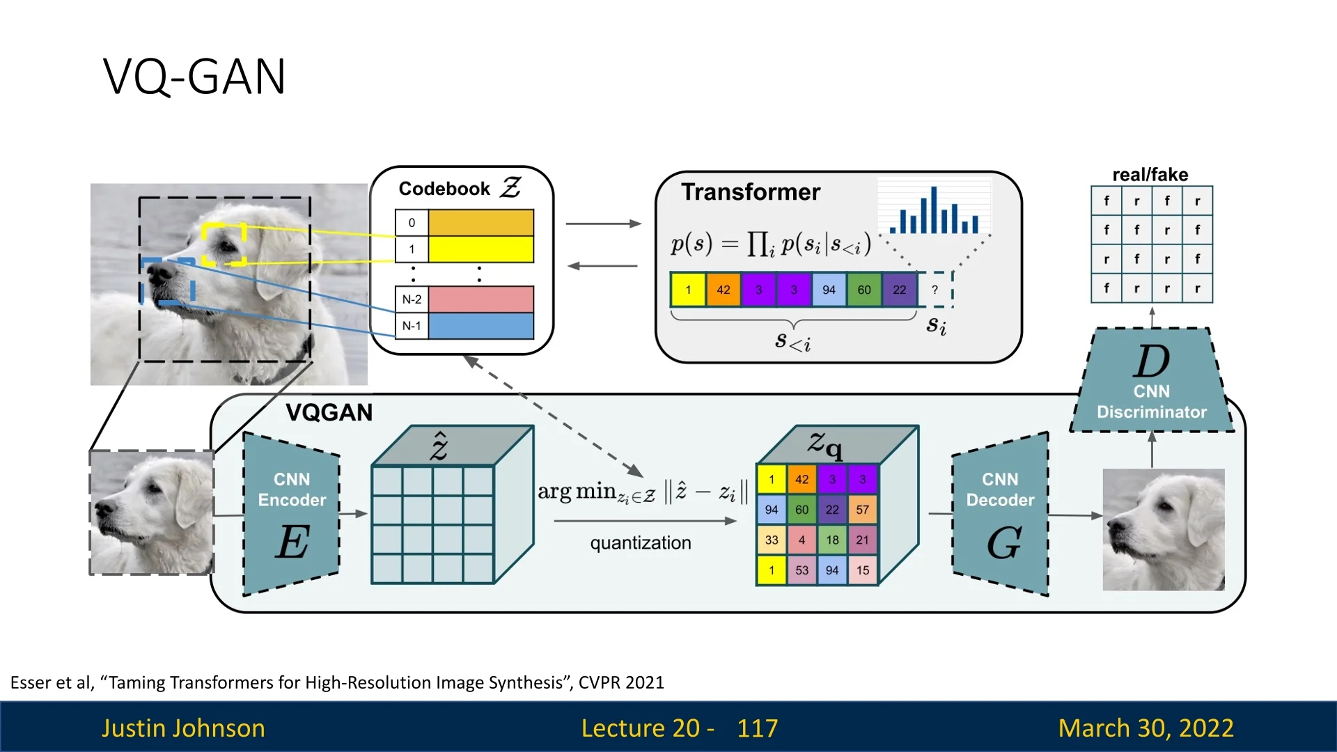
Enrichment 20.7.6.2: Training Objectives and Losses in VQ-GAN
The training of VQ-GAN centers around a perceptually informed autoencoding task. The encoder \( E \) maps an input image \( x \in \mathbb {R}^{H \times W \times 3} \) to a latent map \( \hat {z} = E(x) \in \mathbb {R}^{h \times w \times d} \), which is then quantized to \( z_q \in \mathcal {Z}^{h \times w} \) by nearest-neighbor lookup from a codebook of learned prototypes. The decoder \( G \) reconstructs the image \( \hat {x} = G(z_q) \). While this process resembles the original VQ-VAE [474], the loss function in VQ-GAN is significantly more expressive.
Total Loss The total objective used to train the encoder, decoder, and codebook jointly is: \[ \mathcal {L}_{\mbox{VQ-GAN}} = \lambda _{\mbox{rec}} \cdot \mathcal {L}_{\mbox{rec}} + \lambda _{\mbox{GAN}} \cdot \mathcal {L}_{\mbox{GAN}} + \mathcal {L}_{\mbox{VQ}} \] where each term is detailed below, and \( \lambda _{\mbox{rec}}, \lambda _{\mbox{GAN}} \) are hyperparameters (typically \( \lambda _{\mbox{rec}} = 1.0 \), \( \lambda _{\mbox{GAN}} = 1.0 \)).
1. Perceptual Reconstruction Loss \( \mathcal {L}_{\mbox{rec}} \) Rather than minimizing pixel-wise MSE, VQ-GAN uses a perceptual loss based on deep feature activations: \[ \mathcal {L}_{\mbox{rec}} = \frac {1}{C_l H_l W_l} \left \| \phi _l(x) - \phi _l(\hat {x}) \right \|_2^2 \] Here, \( \phi _l(\cdot ) \) denotes the activation map of a pre-trained VGG network at layer \( l \), and \( C_l, H_l, W_l \) are its dimensions. This encourages reconstructions that preserve semantic and texture-level similarity even if pixel-level details vary, helping avoid the blurriness seen in VQ-VAE outputs.
2. Adversarial Patch Loss \( \mathcal {L}_{\mbox{GAN}} \) To further enhance realism, VQ-GAN adds an adversarial loss using a multi-scale PatchGAN discriminator \( D \). This discriminator classifies local image patches as real or fake. The generator (i.e., encoder + quantizer + decoder) is trained with the hinge loss: \[ \mathcal {L}_{\mbox{GAN}}^{G} = -\mathbb {E}_{\hat {x}} [ D(\hat {x}) ] \quad , \quad \mathcal {L}_{\mbox{GAN}}^{D} = \mathbb {E}_{\hat {x}} [ \max (0, 1 + D(\hat {x})) ] + \mathbb {E}_{x} [ \max (0, 1 - D(x)) ] \] This formulation stabilizes adversarial training and ensures that reconstructions match the patch statistics of real images.
3. Vector Quantization Commitment and Codebook Loss \( \mathcal {L}_{\mbox{VQ}} \) The standard VQ loss is used to train the codebook and encourage encoder outputs to commit to discrete codes. Following [474], the loss is: \[ \mathcal {L}_{\mbox{VQ}} = \underbrace {\left \| \mbox{sg}[E(x)] - z_q \right \|_2^2}_{\mbox{Codebook loss}} + \beta \cdot \underbrace {\left \| E(x) - \mbox{sg}[z_q] \right \|_2^2}_{\mbox{Commitment loss}} \] where \( \mbox{sg}[\cdot ] \) is the stop-gradient operator, and \( \beta \) controls the strength of the commitment penalty (typically \( \beta = 0.25 \)).
Combined Optimization Strategy During training, the encoder, decoder, and codebook are updated to minimize \( \mathcal {L}_{\mbox{VQ-GAN}} \), while the discriminator is trained adversarially via \( \mathcal {L}_{\mbox{GAN}}^{D} \). Optimization alternates between these two steps using Adam with a 2:1 or 1:1 update ratio. The perceptual loss and discriminator feedback reinforce each other: one encourages semantically faithful reconstructions, the other pushes the generator to produce images indistinguishable from real data.
Why This Loss Works The combination of perceptual and adversarial losses compensates for the main weaknesses of prior methods. While VQ-VAE reconstructions are often blurry due to MSE, the perceptual loss helps match high-level content, and adversarial feedback ensures photo-realistic textures. This makes the quantized codebook entries more semantically meaningful, resulting in compressed representations that are useful for downstream transformer modeling.
Training Summary VQ-GAN training proceeds in two stages:
- 1.
- Stage 1: Autoencoding. The encoder, decoder, codebook, and discriminator are trained jointly using the perceptual, adversarial, and quantization losses. The model learns to represent images as discrete token grids with high perceptual quality.
- 2.
- Stage 2: Transformer Language Modeling. The autoencoder is frozen, and a transformer is trained on the flattened token sequences \( z_q \) using standard cross-entropy loss for next-token prediction.
This dual-stage training ensures that VQ-GAN not only compresses visual information effectively, but also produces discrete codes that are highly suitable for transformer-based generation.
Enrichment 20.7.6.3: Discrete Codebooks and Token Quantization
A central innovation in VQ-GAN lies in its use of a discrete latent space, where each spatial location in the encoder output is assigned an index corresponding to a learned codebook entry. This mechanism—first introduced in VQ-VAE [474]—forms the foundation for compressing images into compact, semantically meaningful tokens suitable for transformer-based modeling.
Latent Grid and Codebook Structure Let \( x \in \mathbb {R}^{H \times W \times 3} \) denote an image. The encoder \( E \) transforms it into a continuous latent map \( \hat {z} = E(x) \in \mathbb {R}^{h \times w \times d} \), where each spatial position \( (i, j) \) corresponds to a \( d \)-dimensional vector. The spatial resolution \( h \times w \) is typically much smaller than \( H \times W \), e.g., \( 16 \times 16 \) for \( 256 \times 256 \) images.
This latent map is then quantized into a discrete tensor \( z_q \in \mathcal {Z}^{h \times w} \) using a codebook \( \mathcal {Z} = \{ e_k \in \mathbb {R}^d \mid k = 1, \ldots , K \} \) containing \( K \) learnable embeddings (e.g., \( K = 1024 \)).
Nearest-Neighbor Quantization For each location \( (i,j) \), the vector \( \hat {z}_{i,j} \in \mathbb {R}^d \) is replaced by its closest codebook entry: \[ z_q(i,j) = e_k \quad \mbox{where} \quad k = \arg \min _{k'} \left \| \hat {z}_{i,j} - e_{k'} \right \|_2^2 \] This lookup converts the continuous feature map into a grid of discrete embeddings, each pointing to one of the \( K \) learned codebook vectors.
Gradient Flow via Stop-Gradient and Codebook Updates Because the argmin operation is non-differentiable, VQ-GAN uses the same trick as VQ-VAE: it copies the selected embedding \( e_k \) into the forward pass and blocks gradients from flowing into the encoder during backpropagation. Formally, the quantized output is written as: \[ z_q = \mbox{sg}(e_k) + (\hat {z} - \mbox{sg}(\hat {z})) \] where \( \mbox{sg}(\cdot ) \) denotes the stop-gradient operator.
To update the codebook entries \( \{ e_k \} \), the gradient is backpropagated from the reconstruction loss to the selected embeddings. This allows the codebook to adapt over time based on usage and reconstruction feedback.
Codebook Capacity and Token Usage The number of entries \( K \) in the codebook is a key hyperparameter. A small \( K \) leads to coarse quantization (less expressiveness), while a large \( K \) may overfit or lead to infrequent usage of some codes. VQ-GAN monitors token usage statistics during training to ensure that all codes are being used (via an exponential moving average of codebook assignments). This avoids codebook collapse.
Spatial Token Grid as Transformer Input After quantization, the grid \( z_q \in \mathbb {R}^{h \times w \times d} \) is flattened into a sequence of token indices \( \{k_1, \ldots , k_{hw}\} \in \{1, \ldots , K\}^{hw} \), forming the input for the transformer. The transformer learns to model the autoregressive distribution over this sequence: \[ p(k_1, \ldots , k_{hw}) = \prod _{t=1}^{hw} p(k_t \mid k_1, \ldots , k_{t-1}) \] These discrete tokens serve as the vocabulary of the transformer, analogous to word tokens in natural language processing.
Comparison to VQ-VAE-2 Unlike VQ-VAE-2, which uses multiple hierarchical codebooks to represent coarse-to-fine visual features, VQ-GAN uses a single spatially aligned codebook and compensates for the lack of hierarchy by injecting a stronger perceptual and adversarial training signal. This results in tokens that are rich in local structure and semantically coherent, making them more suitable for transformer-based modeling.
Summary The quantization mechanism in VQ-GAN compresses an image into a spatial grid of discrete tokens drawn from a learned embedding table. This enables efficient transformer training by decoupling high-resolution pixel processing from global token modeling. The next section explains how the transformer is trained on these token sequences to generate new images.
Enrichment 20.7.6.4: Autoregressive Transformer for Token Modeling
Once the VQ-GAN encoder and decoder are trained and the discrete codebook is stabilized, the model proceeds to its second stage: learning a generative model over token sequences. Rather than modeling images at the pixel level, this stage focuses on learning the probability distribution of the codebook indices that describe compressed image representations.
Token Sequence Construction After quantization, the encoder yields a spatial grid of token indices \( z_q \in \{1, \ldots , K\}^{h \times w} \). To apply sequence modeling, this 2D array is flattened into a 1D sequence \( \mathbf {k} = [k_1, \ldots , k_{N}] \), where \( N = h \cdot w \). Typically, this flattening is performed in row-major order, preserving local spatial adjacency as much as possible.
Autoregressive Training Objective A transformer decoder is trained to predict the next token given all previous ones. The learning objective is to maximize the log-likelihood of the true sequence: \[ \mathcal {L}_{\mbox{AR}} = - \sum _{t=1}^{N} \log p(k_t \mid k_1, \ldots , k_{t-1}) \] This objective is optimized using teacher forcing and standard cross-entropy loss. During training, the model is exposed to full sequences (obtained from the pretrained encoder) and learns to predict the next index at each position.
Positional Encoding and Embedding Table To preserve spatial context in the flattened sequence, each token is augmented with a positional encoding. This encoding \( \mbox{PE}(t) \in \mathbb {R}^d \) is added to the learned embedding \( e_{k_t} \), yielding the input to the transformer: \[ x_t = e_{k_t} + \mbox{PE}(t) \] The transformer layers then process this sequence via multi-head self-attention and feed-forward blocks.
Sampling for Image Generation At inference time, the transformer generates a new image by sampling from the learned token distribution:
- 1.
- Initialize with a special start token or random first token.
- 2.
- For \( t = 1 \) to \( N \), sample: \[ k_t \sim p(k_t \mid k_1, \ldots , k_{t-1}) \]
- 3.
- After all tokens are generated, reshape the sequence into a grid \( z_q \in \mathbb {R}^{h \times w} \), look up their embeddings from the codebook, and decode using the frozen VQ-GAN decoder.
Windowed Attention for Long Sequences Modeling large images requires long token sequences (e.g., \( 32 \times 32 = 1024 \) tokens for \( 256 \times 256 \) images). This creates a memory bottleneck for standard transformers due to the quadratic cost of self-attention. To address this, VQ-GAN adopts a sliding window or local attention mechanism: the transformer only attends to a fixed-size neighborhood of preceding tokens when predicting the next one. This approximation reduces computational complexity while preserving local coherence.
Comparison with Pixel-Level Modeling Unlike models that operate directly on pixels (e.g., PixelCNN or autoregressive GANs), this token-based approach offers:
- Lower sequence length: Tokens are downsampled representations, so fewer steps are needed.
- Higher abstraction: Each token represents a meaningful visual chunk (e.g., a part of an object), not just an individual pixel.
- Improved generalization: The transformer learns compositional rules over high-level image structure, rather than low-level noise.
Transformer Variants: Decoder-Only and Encoder–Decoder
The VQ-GAN framework employs different types of transformer architectures depending on the downstream task—ranging from autoregressive image generation to conditional image synthesis from natural language. The two primary transformer types are:
-
Decoder-only (GPT-style) Transformers: For unconditional and class-conditional image generation, VQ-GAN uses a causal decoder transformer inspired by GPT-2 [511]. This architecture models the token sequence left-to-right, predicting each token conditioned on the preceding tokens \(1, \cdots k\). It consists of stacked self-attention blocks with masked attention to preserve causality. The output is a probability distribution over codebook indices for the next token, enabling sequence generation via sampling. This design supports:
- Unconditional generation from a start-of-sequence token
- Class-conditional generation by appending a class token or embedding
-
Encoder–Decoder Transformers (Text-to-Image): For conditional generation from textual descriptions, the authors adopt a full Transformer encoder–decoder architecture—popularized by models like T5 [517] and BART [334]. Here, the encoder processes a sequence of text tokens (from a caption), typically encoded via pretrained embeddings (e.g., CLIP or BERT). The decoder then autoregressively generates image token sequences conditioned on the encoder output. This setup allows for:
- Cross-modal alignment between text and image
- Rich semantic guidance at every generation step
- Enhanced sample quality and relevance in text-to-image tasks
In both cases, the transformer operates over a compressed latent space of visual tokens, not pixels. This architectural choice drastically reduces sequence length (e.g., 16 × 16 = 256 16×16=256 tokens for 256 × 256 256×256 images), enabling efficient training while preserving global structure.
The authors also explore sliding-window attention during inference to reduce quadratic attention costs for long token sequences. This allows the model to scale beyond 256×256 resolution while maintaining tractability.
Training Setup All transformer variants are trained after the VQ-GAN encoder and decoder are frozen. The transformer is optimized using standard cross-entropy loss over codebook indices and trained to minimize next-token prediction error. This decoupling of training stages avoids instability and allows plug-and-play use of any transformer model atop a trained VQ-GAN tokenizer.
Summary The transformer in VQ-GAN learns an autoregressive model over discrete image tokens produced by the encoder and codebook. Its outputs—sequences of token indices—are used to synthesize novel images by decoding through the frozen decoder. In the next subsection, we explore the sampling process in detail and the role of quantization grid size in the fidelity and flexibility of the model.
Enrichment 20.7.6.5: Token Sampling and Grid Resolution
Once a transformer has been trained to model the distribution over token sequences, we can generate new images by sampling from this model. This process involves autoregressively generating a sequence of discrete token indices, reshaping them into a spatial grid, and then decoding them through the frozen decoder network.
Autoregressive Sampling Pipeline At inference time, generation proceeds as follows:
- 1.
- Start from a special start token or a randomly selected token index.
- 2.
- For each timestep \( t \in \{1, \ldots , N\} \), sample the next token index from the model’s predicted distribution: \[ k_t \sim p(k_t \mid k_1, \ldots , k_{t-1}) \]
- 3.
- After all \( N = h \cdot w \) tokens have been generated, reshape the sequence back to a 2D spatial grid.
- 4.
- Look up each token’s codebook embedding and pass the resulting tensor through the decoder to obtain the final image.
This sampling process is computationally expensive, as each new token depends on all previously generated tokens. For longer sequences (e.g., \(32 \times 32 = 1024\) tokens), decoding can be slow, especially without optimized parallel inference.
Impact of Latent Grid Resolution The spatial resolution of the latent token grid \( z_q \in \mathbb {R}^{h \times w} \) is determined by the encoder’s downsampling factor. For instance, with a \(4\times \) downsampling per spatial dimension, a \(256 \times 256\) image is compressed into a \(64 \times 64\) token grid. Larger \( h \times w \) grids provide finer granularity but also lead to longer token sequences for the transformer to model.
There is a trade-off here:
- Higher spatial resolution allows for more detailed reconstructions, especially at high image resolutions.
- Lower spatial resolution results in faster training and sampling but may lead to coarser images.
The authors of VQ-GAN found that using a \(16 \times 16\) token grid worked well for \(256 \times 256\) images, balancing model efficiency and output quality. However, when working with higher-resolution images, grid size becomes a bottleneck: the more aggressively the encoder downsamples, the more difficult it becomes to preserve fine spatial detail. On the other hand, increasing token count burdens the transformer with longer sequences and higher memory demands.
Sliding Window Attention (Optional Variant) To scale to longer sequences without quadratic memory costs, VQ-GAN optionally uses a sliding window attention mechanism. Rather than attending to all previous tokens, each position attends only to a fixed-size window of previous tokens (e.g., the last 256). This approximation significantly reduces memory requirements while preserving local consistency during generation.
Summary Sampling in VQ-GAN is a two-stage process: a transformer generates a sequence of codebook indices that are then decoded into an image. The grid resolution of the quantized latent space plays a critical role in the visual fidelity of outputs and the computational feasibility of training. While smaller grids reduce complexity, larger grids improve detail—highlighting the importance of choosing an appropriate balance for the task at hand.
Enrichment 20.7.6.6: VQ-GAN: Summary and Outlook
VQ-GAN [149] represents a pivotal step in the evolution of generative models by bridging the efficiency of discrete latent modeling with the expressive power of transformers. Its design merges the local inductive strengths of convolutional encoders and decoders with global autoregressive modeling in latent space, enabling synthesis of high-resolution and semantically coherent images. The key ingredients of this system include:
- A convolutional autoencoder with vector quantization to compress high-dimensional images into discrete token grids.
- A codebook trained using perceptual and adversarial losses to produce reconstructions that are sharp and semantically rich.
- An autoregressive transformer that learns to model spatial dependencies among tokens in the latent space, enabling sample generation and manipulation.
Why VQ-GAN Works By introducing adversarial and perceptual supervision into the training of the autoencoder, VQ-GAN overcomes a major limitation of previous models like VQ-VAE and VQ-VAE-2: the tendency toward blurry or oversmoothed reconstructions. The perceptual loss aligns high-level features between generated and ground-truth images, while the patch-based adversarial loss encourages fine detail, particularly texture and edges. Meanwhile, transformers provide a mechanism for globally coherent synthesis by modeling long-range dependencies among latent tokens.
This decoupling of low-level reconstruction and high-level compositionality makes VQ-GAN not only effective but modular. The decoder and transformer can be trained separately, and the codebook can serve as a compact representation for a wide range of downstream tasks.
Future Directions and Influence The modular, tokenized view of image generation introduced by VQ-GAN has had wide-reaching consequences in the field of generative modeling:
- It laid the foundation for powerful text-to-image models like DALLE [525] and followup versions of it, which leverage learned discrete tokens over visual content as a bridge to language.
- The taming-transformers framework became a baseline for generative pretraining and fine-tuning, influencing both the latent diffusion models (LDMs) [548] and modern image editing applications like Stable Diffusion.
- Its discrete latent representation also enabled efficient semantic image manipulation, inpainting, and zero-shot transfer by training lightweight models directly in token space.
In conclusion, VQ-GAN exemplifies how a principled integration of discrete representation learning, adversarial training, and autoregressive modeling can lead to scalable, controllable, and high-fidelity generation. It forms a crucial bridge between convolutional perception and tokenized generative reasoning, and it remains a foundational method in modern generative visual pipelines.
Enrichment 20.8: Additional Important GAN Works
In addition to general-purpose GANs and high-resolution synthesis frameworks, many architectures have been proposed to address specific structured generation tasks—ranging from super-resolution and paired image translation to semantic layout synthesis and motion trajectory forecasting. These models extend adversarial learning to incorporate spatial, semantic, and temporal constraints, often introducing novel conditioning mechanisms, domain priors, and loss formulations.
We begin with seminal architectures such as SRGAN [327] for perceptual super-resolution, pix2pix [266] and CycleGAN [824] for paired and unpaired image translation, SPADE [484] for semantic-to-image generation via spatially-adaptive normalization, and SocialGAN [206] for trajectory prediction in dynamic social environments. These models exemplify how GANs can be tailored to specific applications by redesigning generator–discriminator objectives and conditioning pipelines.
If further exploring recent innovations is of interest, we also recommend reviewing cutting-edge hybrid architectures such as GauGAN2, which fuses semantic maps with text prompts for fine-grained control over scene layout and appearance, and Diffusion-GAN hybrids [707], which combine score-based denoising processes with adversarial training for enhanced realism and robustness. These models reflect emerging trends in generative modeling—blending expressive priors, multimodal conditioning, and stable learning strategies across increasingly complex synthesis domains.
We now proceed to analyze the foundational task-specific GANs in greater depth, each marking a significant step forward in aligning generative modeling with real-world objectives.
Enrichment 20.8.1: SRGAN: Photo-Realistic Super-Resolution
SRGAN [327] introduced the first GAN-based framework for perceptual single-image super-resolution, achieving photo-realistic results at \(4\times \) upscaling. Rather than optimizing conventional pixel-level losses such as Mean Squared Error (MSE), which are known to favor high PSNR but overly smooth outputs, SRGAN proposes a perceptual training objective that aligns better with human visual preferences. This objective combines adversarial realism with deep feature similarity extracted from a pre-trained classification network (VGG16).
Motivation and Limitations of Pixel-Wise Supervision Pixel-based metrics such as MSE or L2 loss tend to produce blurry reconstructions, particularly at large upscaling factors (e.g., \(4\times \)), because they penalize even slight misalignments in fine details. If multiple plausible high-resolution reconstructions exist for a single low-resolution input, the network trained with MSE will learn to output the average of those possibilities—resulting in smooth textures and a loss of perceptual sharpness.
While pixel-wise accuracy is mathematically well-defined, it does not always reflect visual fidelity. To address this, SRGAN replaces the MSE loss with a perceptual loss that compares images in a feature space defined by deep activations of a pre-trained VGG16 network. These intermediate features reflect higher-level abstractions (edges, textures, object parts), which are more aligned with how humans perceive image realism.
Why Use VGG-Based Perceptual Loss? The VGG-based content loss compares the reconstructed image \( \hat {I}_{SR} \) and the ground truth image \( I_{HR} \) not at the pixel level, but in the feature space of a neural network trained for image classification.
Concretely, if \( \phi _{i,j}(\cdot ) \) represents the activations at the \( (i,j) \)-th layer of VGG16, then the perceptual loss is defined as: \[ \mathcal {L}_{\mbox{VGG}} = \frac {1}{W H} \sum _{x,y} \left \| \phi _{i,j}(I_{HR})_{x,y} - \phi _{i,j}(\hat {I}_{SR})_{x,y} \right \|_2^2 \] This loss better preserves fine-grained textures and edges, as it penalizes semantic-level mismatches. Although this approach sacrifices raw PSNR scores, it substantially improves perceptual quality.
Architecture Overview The SRGAN generator is a deep convolutional network consisting of:
- An initial \( 9 \times 9 \) convolution followed by Parametric ReLU (PReLU).
- 16 residual blocks, each comprising two \(3 \times 3\) convolutions with PReLU and skip connections.
- A global skip connection from the input to the output of the residual stack.
- Two sub-pixel convolution blocks (pixel shuffling [584]) to increase spatial resolution by a factor of 4 in total. Each block first applies a learned convolution that expands the number of channels by a factor of \( r^2 \), where \( r \) is the upscaling factor. Then, the resulting feature map is rearranged using a pixel shuffle operation that reorganizes the channels into spatial dimensions. This process allows efficient and learnable upsampling while avoiding checkerboard artifacts commonly associated with transposed convolutions. The rearrangement step transforms a tensor of shape \( H \times W \times (r^2 \cdot C) \) into \( (rH) \times (rW) \times C \), effectively increasing image resolution without introducing new spatial operations.
- A final \(9 \times 9\) convolution with Tanh activation to produce the RGB image.
Skip connections are critical to the generator’s stability and learning efficiency. They allow the network to propagate low-frequency structure (e.g., colors, global layout) directly from the input to the output, enabling the residual blocks to focus solely on learning high-frequency textures and refinements. This decomposition aligns well with the structure-versus-detail duality in image synthesis.
Upsampling Strategy: Sub-Pixel Convolution Blocks A core challenge in super-resolution is learning how to upscale low-resolution inputs into high-resolution outputs while preserving structural integrity and synthesizing high-frequency texture. Traditional interpolation methods such as nearest-neighbor, bilinear, or bicubic are non-parametric—they ignore image content and apply fixed heuristics, often producing smooth but unrealistic textures. Learnable alternatives like transposed convolutions introduce adaptive filters but are known to suffer from checkerboard artifacts due to uneven kernel overlap and gradient instability.
To address these limitations, SRGAN employs sub-pixel convolution blocks, first introduced in ESPCN [584]. Rather than directly increasing spatial resolution, the network instead increases the channel dimension of intermediate features. Specifically, given a desired upscaling factor \( r \), the model outputs a tensor of shape \( H \times W \times (C \cdot r^2) \). This tensor is then passed through a deterministic rearrangement operation called the pixel shuffle, which converts it to a higher-resolution tensor of shape \( rH \times rW \times C \). This process can be visualized as splitting the interleaved channels into spatial neighborhoods—each group of \( r^2 \) channels at a given location forms a distinct \( r \times r \) patch in the upsampled output.
Formally, for a given low-resolution feature map \( F \in \mathbb {R}^{H \times W \times (C \cdot r^2)} \), the pixel shuffle operation rearranges it into \( \tilde {F} \in \mathbb {R}^{rH \times rW \times C} \) via: \[ \tilde {F}(r \cdot i + a, r \cdot j + b, c) = F(i, j, c \cdot r^2 + a \cdot r + b) \] for \( i \in [0, H-1], j \in [0, W-1], a, b \in [0, r-1], c \in [0, C-1] \). This operation is non-parametric and fully differentiable.
This upsampling strategy provides several key benefits:
- It keeps most computation in the low-resolution domain, improving speed and memory efficiency.
- Unlike transposed convolutions, it avoids overlapping kernels, which reduces aliasing and checkerboard artifacts.
- Because the convolution preceding the pixel shuffle is learned, the network can generate content-aware and semantically rich upsampling filters.
However, sub-pixel convolution is not without drawbacks. The hard-coded spatial rearrangement makes it less flexible for modeling long-range spatial dependencies, which must be learned indirectly by preceding convolutional layers.
This mechanism is now widely adopted in modern super-resolution networks, where it strikes an effective balance between learnability, visual quality, and computational efficiency.
Discriminator Design The discriminator is a VGG-style fully convolutional network that:
- Applies a sequence of \(3 \times 3\) convolutions with increasing numbers of filters.
- Reduces spatial resolution using strided convolutions (no max pooling).
- Uses LeakyReLU activations and BatchNorm.
- Ends with two dense layers and a final sigmoid activation to classify images as real or fake.
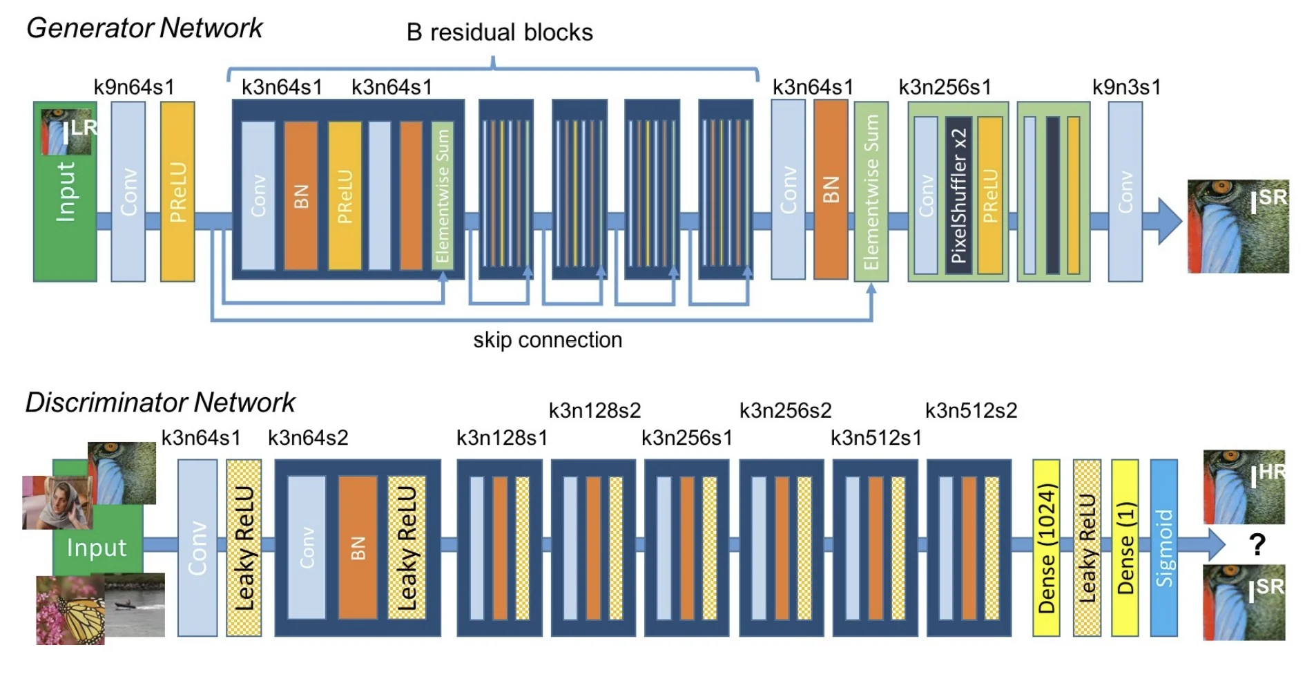
Together, the generator and discriminator are trained in an adversarial framework, where the discriminator learns to distinguish between real and super-resolved images, and the generator learns to fool the discriminator while also minimizing perceptual content loss.
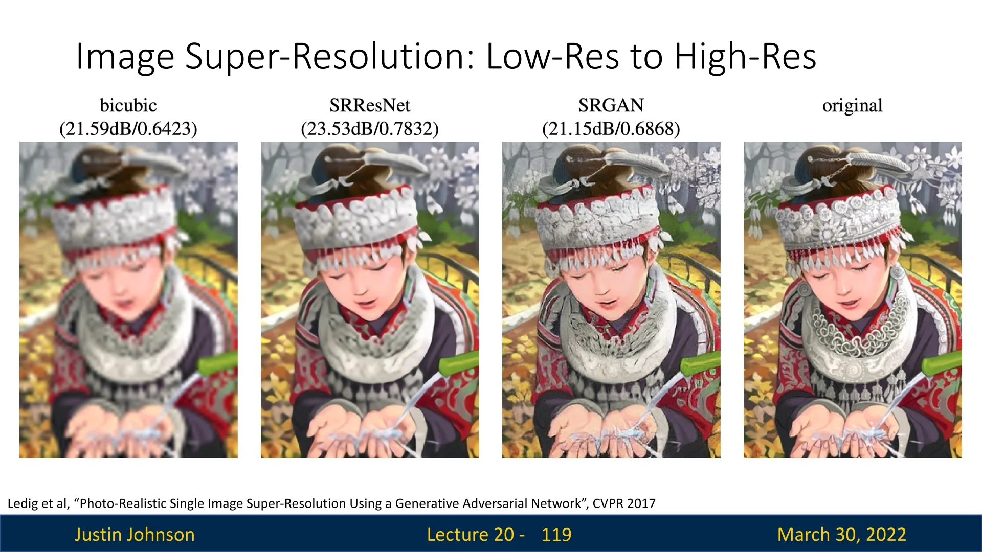
In summary, SRGAN’s perceptual training framework—rooted in feature-level losses and adversarial feedback—transformed the super-resolution landscape. It shifted the focus from purely quantitative fidelity (e.g., PSNR) to perceptual realism, influencing numerous follow-up works in both restoration and generation.
Perceptual Loss Function Let \( \phi _{i,j}(\cdot ) \) denote the feature maps extracted from the \((i,j)\)-th layer of the pretrained VGG19 network. The total perceptual loss used to train SRGAN is: \[ \mathcal {L}_{\mbox{SR}} = \underbrace {\frac {1}{WH} \sum _{x,y} \| \phi _{i,j}(I_{HR})_{x,y} - \phi _{i,j}(\hat {I}_{SR})_{x,y} \|_2^2}_{\mbox{Content Loss (VGG Feature Matching)}} + \lambda \cdot \underbrace {-\log D(\hat {I}_{SR})}_{\mbox{Adversarial Loss}} \] where \( \lambda = 10^{-3} \) balances the two terms.
- Phase 1: Pretrain the generator \( G \) as a ResNet (SRResNet) with MSE loss to produce strong initial reconstructions.
- Phase 2: Jointly train \( G \) and the discriminator \( D \) using the perceptual loss above.
- Generator uses ParametricReLU activations and sub-pixel convolutions [584] for efficient upscaling.
- Discriminator architecture follows DCGAN [510] conventions: LeakyReLU activations, strided convolutions, and no max pooling.
Quantitative and Perceptual Results Despite having lower PSNR than SRResNet, SRGAN consistently achieves higher Mean Opinion Scores (MOS) in human evaluations, indicating more photo-realistic outputs. Tested in experiments on datasets like Set5, Set14, and BSD100.
Enrichment 20.8.2: pix2pix: Paired Image-to-Image Translation with cGANs
Motivation and Formulation The pix2pix framework [266] addresses a family of image-to-image translation problems where we are given paired training data \( \{ (x_i, y_i) \} \), with the goal of learning a mapping \( G: x \mapsto y \) from input images \( x \) (e.g., segmentation masks, sketches, grayscale images) to output images \( y \) (e.g., photos, maps, colored images).
While fully convolutional neural networks (CNNs) can be trained to minimize an L2 or L1 loss between the generated output and the ground truth, such approaches tend to produce blurry results. This is because the pixel-wise losses average over all plausible outputs, failing to capture high-frequency structure or visual realism.
Instead of hand-designing task-specific loss functions, the authors propose using a conditional GAN (cGAN) objective. The discriminator \( D \) is trained to distinguish between real pairs \( (x, y) \) and fake pairs \( (x, G(x)) \), while the generator \( G \) learns to fool the discriminator. This adversarial training strategy encourages the generator to produce outputs that are not just pixel-wise accurate, but also indistinguishable from real images in terms of texture, edges, and fine details.
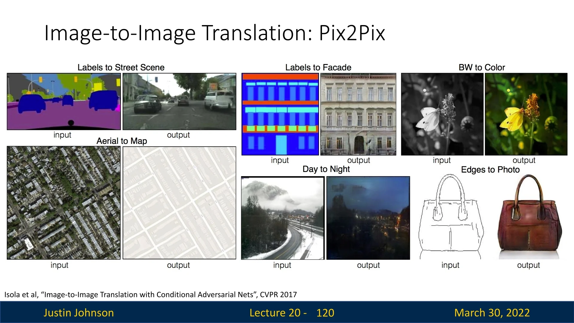
This general-purpose approach enables the same model and training procedure to be applied across a wide range of problems—without modifying the loss function or architecture—highlighting the power of adversarial learning to implicitly learn appropriate loss functions that enforce realism.
Enrichment 20.8.2.1: Generator Architecture and L1 Loss
Generator Architecture: U-Net with Skip Connections The pix2pix generator adopts a U-Net-style encoder–decoder architecture tailored for structured image-to-image translation. Its goal is to transform a structured input image \( x \) (such as an edge map, semantic label mask, or sketch) into a realistic output \( y \), preserving both spatial coherence and semantic fidelity.
A common failure mode of vanilla encoder-decoder CNNs is their tendency to blur or oversmooth outputs. This is because spatial resolution is reduced during encoding, and then the decoder must regenerate fine details from heavily compressed features—often losing important low-level cues such as edges and textures.
To overcome this, pix2pix integrates skip connections that link each encoder layer to its corresponding decoder layer. This structure is inspired by the U-Net architecture originally designed for biomedical segmentation tasks (see §15.6). The idea is to concatenate feature maps from early encoder layers (which contain high-frequency, low-level spatial information) directly into the decoder pathway, providing detailed cues that help the generator synthesize accurate textures, contours, and spatial alignment.
While the architecture is based on U-Net, pix2pix introduces several important differences:
- The generator is trained adversarially as part of a conditional GAN setup, rather than with a pixel-wise classification or regression loss.
- The input–output pairs often differ semantically (e.g., segmentation maps vs. RGB images), requiring stronger representational flexibility.
- Noise is not injected through a latent vector \( z \); instead, pix2pix introduces stochasticity via dropout layers applied at both training and inference time.
This design allows the generator to be both expressive and detail-preserving, making it well-suited for translation tasks where structural alignment between input and output is critical.
The Role of L1 Loss In addition to the adversarial objective, pix2pix uses a pixel-wise L1 loss between the generated image \( G(x) \) and the ground truth image \( y \). Formally, this term is: \[ \mathcal {L}_{L1}(G) = \mathbb {E}_{x,y} \left [ \| y - G(x) \|_1 \right ] \] This loss encourages the generator to output images that are structurally aligned with the target and reduces the risk of mode collapse. The authors argue that L1 is preferable to L2 (mean squared error) because it encourages less blurring. While L2 loss disproportionately penalizes large errors and promotes averaging over plausible solutions (leading to overly smooth results), L1 penalizes errors linearly and retains sharper detail.
The addition of L1 loss provides a simple yet powerful inductive constraint: while the adversarial loss encourages outputs to “look real,” the L1 loss ensures they are aligned with the target. This combination was shown to reduce blurring substantially and is critical for tasks where pixel-level structure matters.
Why Not WGAN or WGAN-GP? While more theoretically grounded adversarial objectives—such as the Wasserstein GAN [14] or WGAN-GP [201]—had already been introduced by the time of pix2pix’s publication, the authors found these alternatives to underperform empirically in their setting.
Specifically, they observed that standard GAN training with a conditional discriminator resulted in sharper edges and more stable convergence across a range of datasets. Therefore, pix2pix adopts the original GAN loss [186], modified for the conditional setting (described in detail in a later section).
Enrichment 20.8.2.2: Discriminator Design and PatchGAN
Discriminator Design and Patch-Level Realism (PatchGAN) In pix2pix, the discriminator is designed to operate at the level of local patches rather than entire images. This design—known as the PatchGAN discriminator—focuses on classifying whether each local region of the output image \( y \) is realistic and consistent with the corresponding region in the input \( x \). Instead of outputting a single scalar value, the discriminator produces a grid of probabilities, one per patch, effectively modeling image realism as a Markov random field.
Architecture: The PatchGAN discriminator is a fully convolutional network that receives as input the concatenation of the input image \( x \) and the output image \( y \) (either real or generated), stacked along the channel dimension. This stacked tensor \( [x, y] \in \mathbb {R}^{H \times W \times (C_x + C_y)} \) is then processed by a series of convolutional layers with stride \(2\), producing a downsampled feature map of shape \( N \times N \), where each value lies in \( [0, 1] \). Each scalar in this output grid corresponds to a specific receptive field (e.g., \(70 \times 70\) pixels in the input image) and reflects the discriminator’s estimate of the realness of that patch—i.e., whether that patch of \( y \), given \( x \), looks realistic and properly aligned.
What the Discriminator Learns: Importantly, the patches that are judged “real” or “fake” come from the output image \( y \), not the input \( x \). The conditioning on \( x \) allows the discriminator to assess whether each region of \( y \) is not only photorealistic but also semantically consistent with the structure of \( x \). This conditioning mechanism is crucial in tasks such as label-to-image translation, where the spatial alignment of objects is important.
Benefits: The PatchGAN discriminator has several advantages:
- It generalizes across image sizes since it is fully convolutional.
- It promotes high-frequency correctness, which encourages the generator to focus on local realism such as textures and edges.
Thus, rather than making a holistic judgment over the entire image, the discriminator acts as a texture and detail critic, applied densely across the image surface.
Objective: The discriminator in pix2pix is trained using the original GAN objective [186], adapted to the conditional setting. The discriminator \( D \) receives both the input image \( x \) and the output image—either the real \( y \sim p_{\mbox{data}}(y \mid x) \) or the generated output \( G(x) \). The discriminator is fully convolutional and produces a spatial grid of predictions rather than a single scalar, making it a PatchGAN.
Each element in the discriminator’s output grid corresponds to a local patch (e.g., \(70 \times 70\) pixels) in the image, and represents the discriminator’s estimate of whether that patch is “real” or “fake,” conditioned on \( x \). The overall discriminator loss is averaged across this grid: \[ \mathcal {L}_{D} = \mathbb {E}_{x,y} \left [ \log D(x, y) \right ] + \mathbb {E}_{x} \left [ \log (1 - D(x, G(x))) \right ] \]
Likewise, the adversarial component of the generator’s objective is: \[ \mathcal {L}_{G}^{\mbox{adv}} = \mathbb {E}_{x} \left [ \log (1 - D(x, G(x))) \right ] \]
Since the outputs of \( D \) are now grids of probabilities (one per receptive field region), the log terms are applied elementwise and the expectation denotes averaging across the training batch and spatial positions. In implementation, this is usually done using a mean over the entire \( N \times N \) output map.
Benefits of Patch-Based Discrimination:
- Reduced complexity: PatchGAN has fewer parameters and is easier to train than a global discriminator.
- High-frequency sensitivity: It is particularly good at enforcing local texture realism and preserving fine-grained detail.
- Fully convolutional: Since the model operates locally, it can be seamlessly applied to images of varying resolution at test time.
In the pix2pix paper, a \(70 \times 70\) receptive field is used, referred to as the \(70\)-PatchGAN, which balances context and texture fidelity. Smaller receptive fields may ignore global structure, while larger fields increase training difficulty and instability.
Having established the adversarial loss, we now examine the L1 reconstruction loss, which complements the discriminator by promoting spatial alignment and reducing blurriness in the generator output. Let me know when you’re ready to continue.
Enrichment 20.8.2.3: Full Training Objective and Optimization
Generator Loss: Combining Adversarial and Reconstruction Objectives While adversarial training encourages realism in the generated outputs, it does not ensure that the output matches the expected ground truth \( y \) in structured tasks such as semantic segmentation or image-to-image translation. For example, without additional supervision, the generator could produce an image that looks realistic but fails to reflect the precise layout or identity present in the input \( x \).
To address this, pix2pix adds an L1 loss between the generated output \( G(x) \) and the target image \( y \). The full generator loss becomes: \[ \mathcal {L}_{G} = \mathcal {L}_{G}^{\mbox{adv}} + \lambda \cdot \mathcal {L}_{\mbox{L1}} \] \[ \mbox{with} \quad \mathcal {L}_{\mbox{L1}} = \mathbb {E}_{x,y} \left [ \| y - G(x) \|_1 \right ] \]
Here, \( \lambda \) is a hyperparameter (typically set to \( \lambda = 100 \)) that balances the trade-off between fidelity to the ground truth and perceptual realism. The L1 loss is preferred over L2 (MSE) because it produces less blurring—a crucial feature for preserving edges and structural alignment.
This combined objective offers the best of both worlds:
- The adversarial loss encourages outputs that reside on the manifold of natural images.
- The L1 loss ensures spatial and semantic coherence between the prediction and the actual output.
The final optimization problem for the generator is: \[ G^* = \arg \min _{G} \max _{D} \mathcal {L}_{\mbox{cGAN}}(G, D) + \lambda \cdot \mathcal {L}_{\mbox{L1}}(G) \] where \( \mathcal {L}_{\mbox{cGAN}} \) denotes the conditional GAN loss using the PatchGAN discriminator: \[ \mathcal {L}_{\mbox{cGAN}}(G, D) = \mathbb {E}_{x,y} \left [ \log D(x, y) \right ] + \mathbb {E}_{x} \left [ \log (1 - D(x, G(x))) \right ] \]
Together, this objective promotes outputs that are not only indistinguishable from real images but also tightly aligned with the conditional input. The addition of L1 loss proved essential for stabilizing training, especially early in optimization when adversarial feedback is still weak or noisy.
We now conclude this overview of pix2pix with a summary of the use cases and real-world applications from the original paper.
Enrichment 20.8.2.4: Summary and Generalization Across Tasks
The core insight of pix2pix [266] is that many structured prediction tasks in computer vision—such as semantic segmentation, edge-to-photo conversion, and sketch-to-image generation—can be unified under the framework of conditional image translation. Rather than hand-designing task-specific loss functions, the GAN-based strategy learns a loss function implicitly through the discriminator, trained to judge how well an output image matches the target distribution given the input.
This conditional GAN setup—combined with a strong L1 reconstruction prior and a PatchGAN discriminator—proved surprisingly effective across a wide variety of domains. Figure 20.50 showcases representative examples from the original paper across multiple datasets and tasks.
Importantly, the pix2pix framework assumes access to paired training data—i.e., aligned input–output image pairs \( (x, y) \). In practice, however, such datasets are often expensive or infeasible to collect. For instance, we might have access to photos of horses and zebras, but no one-to-one mapping between them.
This limitation motivated a follow-up line of research into unpaired image-to-image translation, where models learn to transfer style, texture, or semantics between two domains without explicitly aligned data. The seminal work in this space is CycleGAN [824], which we explore next. It introduces a cycle-consistency loss that allows training without paired examples, opening the door to powerful translation tasks such as horse-to-zebra, summer-to-winter, and Monet-to-photo.
Enrichment 20.8.3: CycleGAN: Unpaired Image-to-Image Translation
Enrichment 20.8.3.1: Motivation: Beyond Paired Supervision in Image Translation
While pix2pix (see Enrichment 20.8.1) demonstrated the power of conditional GANs for paired image-to-image translation, its applicability is fundamentally limited by the need for aligned training pairs \((x, y)\)—that is, input images and their exact corresponding target images. In many practical domains, such as translating between artistic styles, seasons, or weather conditions, paired data is either unavailable or prohibitively expensive to collect.
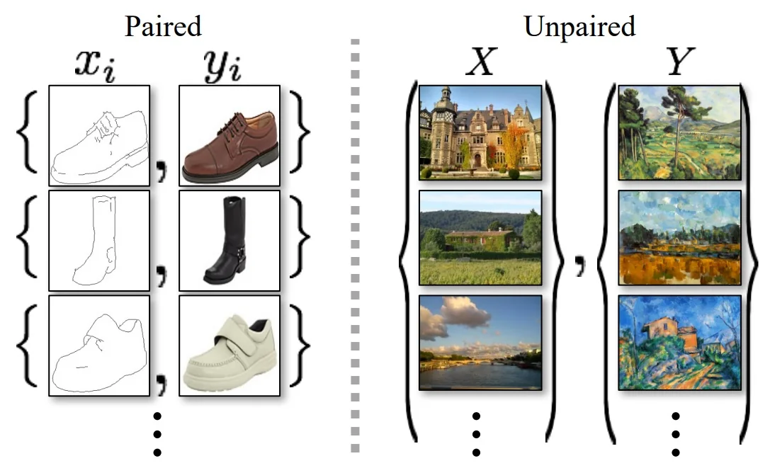
CycleGAN [824] tackles this challenge by proposing an unsupervised framework that learns mappings between two visual domains \(X\) and \(Y\) using only unpaired collections of images from each domain. The central question becomes: How can we learn a function \(G: X \to Y\) when no direct correspondences exist?
Key Insight: Cycle Consistency
At the heart of CycleGAN is the cycle consistency constraint, a principle that enables learning from unpaired datasets. The system consists of two generators: \( G: X \rightarrow Y \), which maps images from domain \( X \) to domain \( Y \), and \( F: Y \rightarrow X \), which learns the reverse mapping.
The intuition is that if we start with an image \( x \) from domain \( X \), translate it to \( Y \) via \( G \), and then map it back to \( X \) via \( F \), the reconstructed image \( F(G(x)) \) should closely resemble the original \( x \). Likewise, for any \( y \in Y \), \( G(F(y)) \approx y \). This cycle consistency enforces that neither mapping is allowed to lose or invent too much information: the transformations should be approximately invertible and content-preserving.
Why does this help with unpaired data? Without paired supervision, there are infinitely many functions that can map the distribution of \( X \) to \( Y \) in a way that fools a GAN discriminator. However, most such mappings would destroy the underlying content, yielding images that are realistic in appearance but semantically meaningless. By explicitly requiring \( F(G(x)) \approx x \) and \( G(F(y)) \approx y \), CycleGAN dramatically restricts the space of possible solutions.
The network learns to transfer style while keeping the essential structure or identity intact, making unsupervised image-to-image translation feasible.
Enrichment 20.8.3.2: Typical Use Cases
CycleGAN’s framework has been widely adopted in domains where paired data is scarce or unavailable, including:
- Artistic style transfer (e.g., photographs \(\leftrightarrow \) Monet or Van Gogh paintings)
- Season or weather translation (e.g., summer \(\leftrightarrow \) winter, day \(\leftrightarrow \) night)
- Object transfiguration (e.g., horse \(\leftrightarrow \) zebra, apple \(\leftrightarrow \) orange)
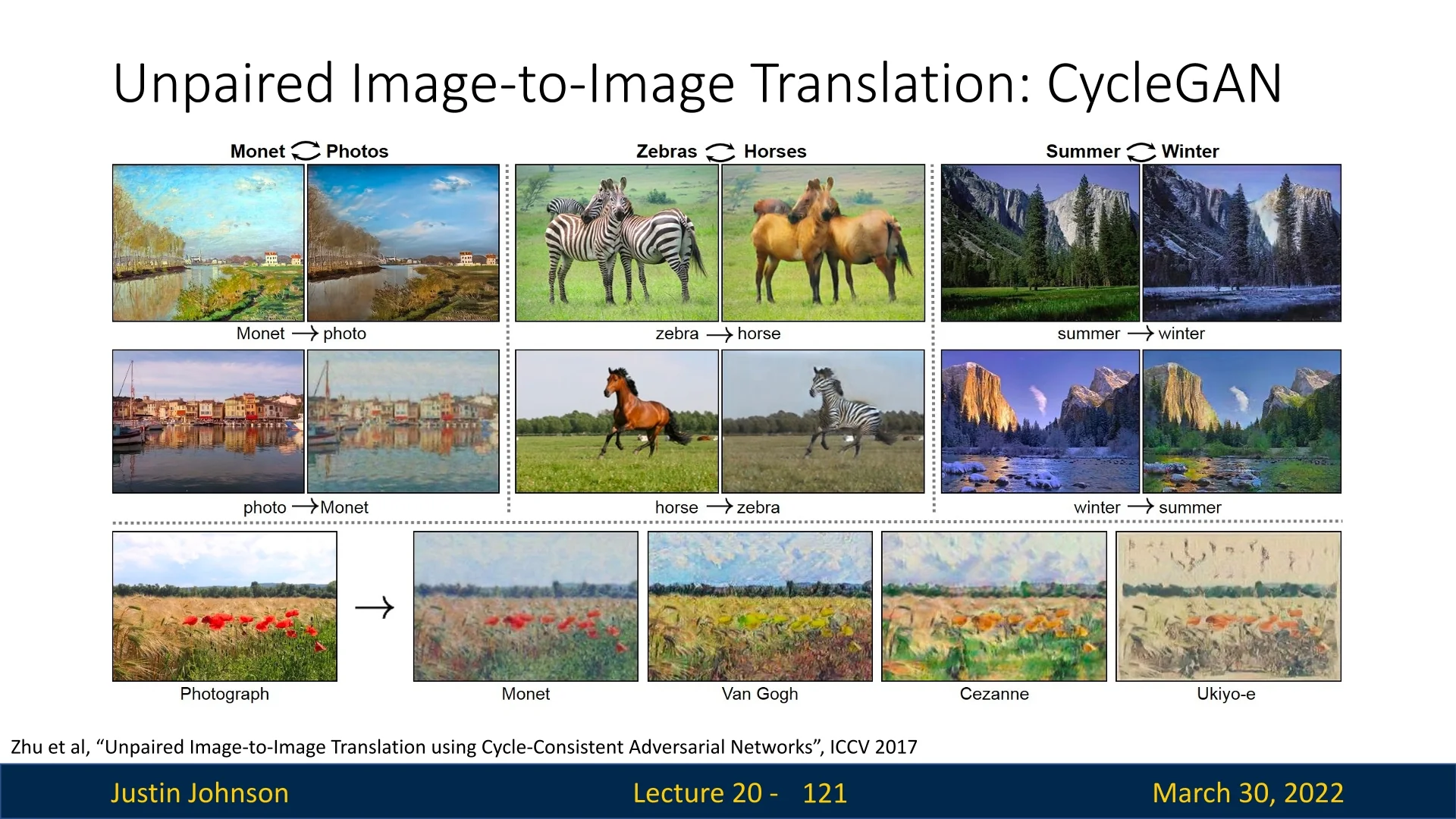
Caution: Although CycleGAN and similar generative methods have attracted attention in medical imaging (e.g., MRI \(\leftrightarrow \) CT translation), their use in this context is highly controversial and potentially dangerous. There is growing evidence in the literature and community commentaries that generative models can hallucinate critical features—such as tumors or lesions—that do not exist in the real patient scan, or fail to preserve vital diagnostic information. Thus, care must be taken to avoid uncritical or clinical use of unpaired translation networks in safety-critical domains; for further discussion, see [112, 758].
This motivation sets the stage for the architectural design and learning objectives of CycleGAN, which we discuss next.
Enrichment 20.8.3.3: CycleGAN Architecture: Dual Generators and Discriminators
CycleGAN consists of two generators and two discriminators:
- Generator \( G: X \rightarrow Y \): Translates an image from domain \( X \) (e.g., horse) to domain \( Y \) (e.g., zebra).
- Generator \( F: Y \rightarrow X \): Translates an image from domain \( Y \) back to domain \( X \).
- Discriminator \( D_Y \): Distinguishes between real images \( y \) in domain \( Y \) and generated images \( G(x) \).
- Discriminator \( D_X \): Distinguishes between real images \( x \) in domain \( X \) and generated images \( F(y) \).
Each generator typically uses an encoder–decoder architecture with residual blocks, while the discriminators are PatchGANs (see enrichment 20.8.2.2.0), focusing on local realism rather than global classification.
The dual generator–discriminator setup allows CycleGAN to simultaneously learn both forward and reverse mappings, supporting unsupervised translation in both directions.
Enrichment 20.8.3.4: CycleGAN: Loss Functions and Training Objectives
Adversarial Loss: Least Squares GAN (LSGAN)
A central goal in CycleGAN is to ensure that each generator produces images that are indistinguishable from real images in the target domain. Rather than relying on the standard GAN log-likelihood loss, CycleGAN adopts the Least Squares GAN (LSGAN) objective [429], which stabilizes training and yields higher-fidelity results.
For generator \(G: X \rightarrow Y\) and discriminator \(D_Y\), the LSGAN adversarial loss is: \[ \mathcal {L}_{\mbox{GAN}}^{\mbox{LS}}(G, D_Y, X, Y) = \mathbb {E}_{y \sim p_{\mbox{data}}(y)} \left [ (D_Y(y) - 1)^2 \right ] + \mathbb {E}_{x \sim p_{\mbox{data}}(x)} \left [ (D_Y(G(x)))^2 \right ] \] This encourages the discriminator to output 1 for real images and 0 for fake (generated) images. Simultaneously, the generator is trained to fool the discriminator by minimizing: \[ \mathcal {L}_G^{\mbox{LS}} = \mathbb {E}_{x \sim p_{\mbox{data}}(x)} \left [ (D_Y(G(x)) - 1)^2 \right ] \] An identical adversarial loss is used for the reverse mapping (\(F: Y \rightarrow X\), \(D_X\)). The least squares loss is empirically more stable and less prone to vanishing gradients than the original log-loss formulation.
Cycle Consistency Loss
The cycle consistency loss is what enables learning with unpaired data. If we translate an image from domain \(X\) to \(Y\) via \(G\), and then back to \(X\) via \(F\), we should recover the original image: \(F(G(x)) \approx x\). The same logic holds for the reverse direction, \(G(F(y)) \approx y\). This is enforced via an L1 loss: \[ \mathcal {L}_{\mbox{cyc}}(G, F) = \mathbb {E}_{x \sim p_{\mbox{data}}(x)} \left [ \| F(G(x)) - x \|_1 \right ] + \mathbb {E}_{y \sim p_{\mbox{data}}(y)} \left [ \| G(F(y)) - y \|_1 \right ] \] The use of L1 loss (mean absolute error) in CycleGAN is deliberate and particularly suited for image reconstruction tasks. While L2 loss (mean squared error) is commonly used in regression settings, it has the tendency to penalize large errors more harshly and to average out possible solutions. In the context of image translation, this averaging effect often leads to over-smoothed and blurry outputs, especially when multiple plausible reconstructions exist.
In contrast, L1 loss treats all deviations linearly and is less sensitive to outliers, which makes it better at preserving sharp edges, fine details, and local structure in the generated images. Empirically, optimizing with L1 encourages the network to maintain crisp boundaries and avoids the tendency of L2 to ”wash out” high-frequency content. As a result, L1 loss is a better fit for the cycle consistency objective, promoting reconstructions that are visually sharper and closer to the original input.
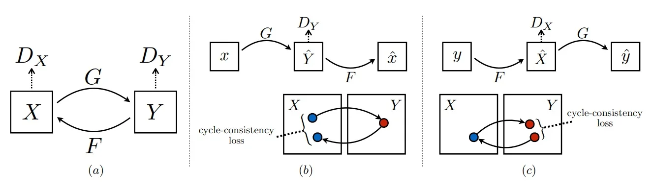
Identity Loss (Optional)
To further regularize the mappings—especially when color or global content should remain unchanged (e.g., in style transfer)—CycleGAN optionally employs an identity loss: \[ \mathcal {L}_{\mbox{identity}}(G, F) = \mathbb {E}_{y \sim p_{\mbox{data}}(y)} \left [ \| G(y) - y \|_1 \right ] + \mathbb {E}_{x \sim p_{\mbox{data}}(x)} \left [ \| F(x) - x \|_1 \right ] \] This penalizes unnecessary changes to images already in the target domain.
Summary
The adversarial losses ensure that generated images in both directions are indistinguishable from real samples, while the cycle consistency and (optionally) identity losses force the learned mappings to preserve core content and structure. The overall objective is a weighted sum of these components: \[ \mathcal {L}_{\mbox{total}}(G, F, D_X, D_Y) = \mathcal {L}_{\mbox{GAN}}^{\mbox{LS}}(G, D_Y, X, Y) + \mathcal {L}_{\mbox{GAN}}^{\mbox{LS}}(F, D_X, Y, X) + \lambda _{\mbox{cyc}} \mathcal {L}_{\mbox{cyc}}(G, F) + \lambda _{\mbox{id}} \mathcal {L}_{\mbox{identity}}(G, F) \] where \(\lambda _{\mbox{cyc}}\) and \(\lambda _{\mbox{id}}\) are hyperparameters.
Enrichment 20.8.3.5: Network Architecture and Practical Training Considerations
Generator and Discriminator Architectures
Generators: CycleGAN employs a ResNet-based generator for both \(G: X \rightarrow Y\) and \(F: Y \rightarrow X\). Each generator typically consists of an initial convolutional block, followed by several residual blocks (commonly 6 or 9, depending on image size), and a set of upsampling (deconvolution) layers. Instance normalization and ReLU activations are used throughout to stabilize training and promote style flexibility. The design is chosen to enable both global and local transformations while maintaining content structure.
Discriminators: Both \(D_X\) and \(D_Y\) use a PatchGAN architecture—identical in spirit to the discriminator design in pix2pix (see Section Enrichment 20.8.1). Instead of classifying the entire image as real or fake, PatchGAN outputs a grid of real/fake probabilities, each associated with a spatial patch (e.g., \(70 \times 70\) pixels) in the input. This local focus encourages preservation of texture and style across the translated images, without requiring global image-level pairing.
Normalization and Activation: CycleGAN replaces batch normalization with instance normalization (see §7.14), which is especially beneficial for style transfer and image translation tasks. Unlike batch normalization, which normalizes feature statistics across the batch dimension, instance normalization computes the mean and variance independently for each sample and each channel, but only across the spatial dimensions \((H \times W)\). Specifically, for a given sample \(n\) and channel \(c\), instance normalization calculates: \[ \mu _{n,c} = \frac {1}{HW} \sum _{h=1}^{H} \sum _{w=1}^{W} x_{n,c,h,w}, \qquad \sigma ^2_{n,c} = \frac {1}{HW} \sum _{h=1}^{H} \sum _{w=1}^{W} \left (x_{n,c,h,w} - \mu _{n,c}\right )^2 \] and normalizes accordingly. This operation decouples the feature scaling from the batch and instead focuses normalization on the statistics of each individual sample and channel. As a result, instance normalization improves the consistency of style adaptation and translation, making it particularly well-suited for CycleGAN and similar works.
Training Strategy and Hyperparameters
The training procedure alternates between updating the generators (\(G\), \(F\)) and the discriminators (\(D_X\), \(D_Y\)). The total objective is a weighted sum of adversarial loss, cycle-consistency loss, and (optionally) identity loss: \[ \mathcal {L}_{\mbox{CycleGAN}} = \mathcal {L}_{\mbox{GAN}}(G, D_Y, X, Y) + \mathcal {L}_{\mbox{GAN}}(F, D_X, Y, X) + \lambda _{\mbox{cyc}}\mathcal {L}_{\mbox{cyc}}(G, F) + \lambda _{\mbox{id}}\mathcal {L}_{\mbox{identity}}(G, F) \] where \(\lambda _{\mbox{cyc}}\) and \(\lambda _{\mbox{id}}\) are hyperparameters controlling the importance of cycle and identity losses. Empirically, \(\lambda _{\mbox{cyc}} = 10\) is standard, and \(\lambda _{\mbox{id}}\) is set to \(0\) or \(0.5\) depending on the task.
Optimizers: CycleGAN uses the Adam optimizer, with \(\beta _1 = 0.5\) and \(\beta _2 = 0.999\), which are well-suited for stabilizing adversarial training.
Unpaired Data Setup: During each epoch, the model draws random samples from unpaired sets \(X\) and \(Y\), so every batch contains independently sampled images from both domains. This setup, along with cycle-consistency, enables effective learning without paired supervision.
Stabilizing Discriminator Training with a Fake Image Buffer To further stabilize adversarial training, CycleGAN maintains a buffer of previously generated fake images (typically 50) for each domain. When updating the discriminator, a random sample from this buffer is mixed with the most recent generated images. This approach prevents the discriminator from overfitting to the generator’s most current outputs, introduces greater diversity in the fake set, and improves convergence.
Enrichment 20.8.3.6: Ablation Study: Impact of Loss Components in CycleGAN
A comprehensive ablation study in CycleGAN systematically investigates the roles of the GAN loss, cycle-consistency loss, and their combinations. The results, as reported in the original CycleGAN paper [824], demonstrate that both adversarial (GAN) and cycle-consistency losses are critical for successful unpaired image-to-image translation.
Effect of Removing Loss Components
- Removing the GAN loss (using only cycle-consistency) produces outputs with preserved content but poor realism; the results lack natural appearance and often fail to match the target domain visually.
- Removing the cycle-consistency loss (using only adversarial loss) leads to mode collapse and lack of content preservation. The model may generate realistic-looking images, but they are often unrelated to the input and fail to capture the source structure.
- Cycle loss in only one direction (e.g., forward \(F(G(x)) \approx x\) or backward \(G(F(y)) \approx y\)) is insufficient and frequently causes training instability and mode collapse. The ablation reveals that bidirectional cycle consistency is essential for learning meaningful mappings without paired data.
Quantitative Results (from the CycleGAN Paper) The ablation is quantified using semantic segmentation metrics (per-pixel accuracy, per-class accuracy, and class IoU) evaluated on the Cityscapes dataset for both labels \(\rightarrow \) photo and photo \(\rightarrow \) labels directions. Tables 20.4 and 20.5 are directly reproduced from [824].
| Loss | Per-pixel acc. | Per-class acc. | Class IOU |
|---|---|---|---|
| Cycle alone | 0.22 | 0.07 | 0.02 |
| GAN alone | 0.51 | 0.11 | 0.08 |
| GAN + forward cycle | 0.55 | 0.18 | 0.12 |
| GAN + backward cycle | 0.39 | 0.14 | 0.06 |
| CycleGAN | 0.52 | 0.17 | 0.11 |
| Loss | Per-pixel acc. | Per-class acc. | Class IOU |
|---|---|---|---|
| Cycle alone | 0.10 | 0.05 | 0.02 |
| GAN alone | 0.53 | 0.11 | 0.07 |
| GAN + forward cycle | 0.49 | 0.11 | 0.07 |
| GAN + backward cycle | 0.01 | 0.06 | 0.01 |
| CycleGAN | 0.58 | 0.22 | 0.16 |
Qualitative Analysis The following figure visually compares the effects of different loss combinations. Removing either the GAN or cycle-consistency component leads to images that either lack realism (cycle alone) or ignore input structure (GAN alone, or single-direction cycle loss). The full CycleGAN model (with both losses in both directions) produces outputs that are both photorealistic and semantically aligned with the input.
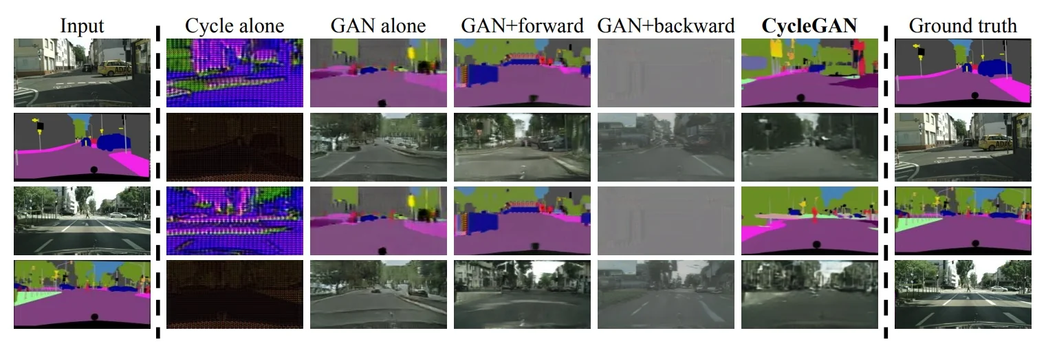
Summary The ablation study conclusively shows that both adversarial and cycle-consistency losses are indispensable for successful unpaired image-to-image translation. The combination ensures the generated outputs are realistic, diverse, and semantically faithful to their source images, while avoiding mode collapse and degenerate mappings.
Enrichment 20.8.3.7: Summary and Transition to Additional Generative Approaches
The innovations introduced by CycleGAN have inspired a diverse ecosystem of task-specific GAN models, each adapting adversarial training to new modalities and challenges. Notable such works we won’t cover in-depth include:
- SPADE [484]: Semantic image synthesis using spatially-adaptive normalization, which achieves high-resolution generation from segmentation maps.
- SocialGAN [206]: Multimodal trajectory forecasting for socially-aware path prediction in crowds.
- MoCoGAN/VideoGAN [109]: Adversarial video generation architectures for modeling temporal dynamics in complex scenes.
Together, these models demonstrate the flexibility of adversarial learning in structured generation tasks. In the following sections, we broaden our view beyond GANs to introduce new families of generative approaches—including diffusion models and flow matching—that are rapidly advancing the state of the art in image, video, and sequential data synthesis.
Enrichment 20.9: Diffusion Models: Modern Generative Modeling
Enrichment 20.9.0.1: Motivation: Limitations of Previous Generative Models
Diffusion models have emerged as a powerful and principled approach to generative modeling, effectively addressing several longstanding challenges found in earlier generative paradigms. To appreciate their significance, it helps to briefly revisit these earlier approaches and clearly identify their main limitations:
Autoregressive Models (PixelCNN, PixelRNN, ...) Autoregressive models factorize the joint probability distribution into sequential conditional predictions, enabling exact likelihood computation and precise modeling of pixel-level dependencies. However, their inherently sequential nature severely limits sampling speed, making high-resolution synthesis prohibitively slow. Moreover, their reliance on local receptive fields often restricts global coherence and makes long-range dependencies difficult to model efficiently.
Variational Autoencoders (VAEs) VAEs provide efficient inference through latent variable modeling and offer stable training and sampling. Nonetheless, the assumption of independent Gaussian likelihoods at the output leads to blurred images and limited sharpness. Additionally, VAEs are vulnerable to posterior collapse, where the latent representation becomes underutilized, reducing expressivity and diversity in generated outputs.
Generative Adversarial Networks (GANs) GANs achieve impressive realism by optimizing an adversarial objective, bypassing explicit likelihood computation. Despite their success, GANs notoriously suffer from instability during training, sensitivity to hyperparameters, and mode collapse, where the generator focuses on a narrow subset of the data distribution. Furthermore, their lack of explicit likelihood estimation complicates evaluation and interpretability.
Hybrid Approaches (VQ-VAE, VQ-GAN) Hybrid models such as VQ-VAE and VQ-GAN combine discrete latent representations with autoregressive or adversarial priors. These methods partially address the shortcomings of VAEs and GANs but introduce their own issues, such as quantization artifacts, limited expressivity due to often codebook collapse, and computational inefficiency in latent space sampling.
The Case for Diffusion Models Diffusion models naturally overcome many of the above limitations by modeling data generation as the gradual reversal of a diffusion (noise-adding) process. Specifically, they offer:
- Stable and Robust Training: Diffusion models avoid adversarial training entirely, leading to stable and reproducible optimization.
- Explicit Likelihood Estimation: Their probabilistic framework supports tractable likelihood estimation, aiding interpretability, evaluation, and theoretical understanding.
- High-Quality and Diverse Generation: Iterative refinement through small denoising steps enables sharp, coherent outputs comparable to GANs, without common GAN instabilities.
- Flexible and Parallelizable Sampling: Recent advances (e.g., DDIM [600]) have accelerated inference significantly, improving practical utility compared to autoregressive and hybrid approaches.
Enrichment 20.9.1: Introduction to Diffusion Models
Diffusion models represent a rigorous class of probabilistic generative models that transform data generation into the problem of reversing a gradual, structured corruption process. Inspired by nonequilibrium thermodynamics [598], these models define a stochastic Markov chain that systematically injects noise into a data sample over many steps—the forward process—until the data is fully randomized. The core learning objective is to parameterize and learn the reverse process: a denoising Markov chain capable of synthesizing realistic data by iteratively refining pure noise back into structured samples. This framework elegantly sidesteps many pitfalls of earlier generative models—such as adversarial collapse in GANs and latent mismatch in VAEs—by relying on explicit, tractable likelihoods and theoretically grounded transitions.
Mathematical Foundation and Dual Processes At the heart of diffusion models are two complementary stochastic processes, each defined with mathematical precision:
-
Forward Process (Diffusion, Corruption):
Let \(\mathbf {x}_0\) be a clean data sample (such as an image). Diffusion-based generative models transform this data into pure noise through a gradual, multi-step corruption process. This is implemented as a Markov chain : \[ \mathbf {x}_0 \rightarrow \mathbf {x}_1 \rightarrow \cdots \rightarrow \mathbf {x}_T, \] where at each timestep \(t\), Gaussian noise is added to slightly degrade the signal. The transition kernel \(q(\mathbf {x}_t \mid \mathbf {x}_{t-1})\) is a probability density function, not a discrete probability. It assigns a scalar density value to a potential noisy state \(\mathbf {x}_t\); a high density indicates that \(\mathbf {x}_t\) is a likely result of adding noise to \(\mathbf {x}_{t-1}\), while a low density implies it is statistically inconsistent with the noise model.
Formally, this transition is defined as a multivariate Gaussian: \begin {equation} q(\mathbf {x}_t \mid \mathbf {x}_{t-1}) = \mathcal {N}\left (\mathbf {x}_t;\, \underbrace {\sqrt {1 - \beta _t} \, \mathbf {x}_{t-1}}_{\mbox{Mean } \boldsymbol {\mu }},\, \underbrace {\beta _t \mathbf {I}}_{\mbox{Covariance } \boldsymbol {\Sigma }} \right ). \label {eq:chapter20_forward_step_detailed} \end {equation} This notation specifies three key components:
- 1.
- Subject (\(\mathbf {x}_t\)): The variable whose likelihood we are measuring.
- 2.
- Mean (\(\boldsymbol {\mu } = \sqrt {1 - \beta _t} \, \mathbf {x}_{t-1}\)): The expected value of the new state. Note that the previous state \(\mathbf {x}_{t-1}\) is scaled down by \(\sqrt {1 - \beta _t}\).
- 3.
- Covariance (\(\boldsymbol {\Sigma } = \beta _t \mathbf {I}\)): The spread of the injected noise, controlled by the scalar \(\beta _t \in (0, 1)\) and the identity matrix \(\mathbf {I}\).
Design Choices: Stability, Structure, and Tractability
The specific mathematical formulation of the forward process is not arbitrary; it relies on careful design choices that ensure the process is stable, computationally tractable, and theoretically sound.
-
Why Diagonal Covariance (\(\beta _t \mathbf {I}\))?
To understand this choice, we must distinguish between what a covariance matrix can do and what the diffusion model chooses to do. With a flattened image vector of size \(D\), the covariance matrix is a \(D \times D\) grid. Using \(\beta _t \mathbf {I}\) simplifies this into two distinct properties:
-
Uniformity vs. Variable Noise (Isotropy): Mathematically, the diagonal elements of a covariance matrix \((\Sigma _{ii})\) control the variance (noise power) for each individual pixel. We could set these values differently—for instance, adding high variance to the background pixels and low variance to the subject.
However, standard diffusion approach uses the scalar \(\beta _t\) to force every diagonal element to be identical: \[ \Sigma = \begin {bmatrix} \beta _t & 0 & \cdots \\ 0 & \beta _t & \cdots \\ \vdots & \vdots & \ddots \end {bmatrix} \] This choice enforces equal opportunity degradation. Since we do not know a priori which pixels are important, we degrade every pixel with the exact same intensity. If we used variable noise, the model might learn to ignore high-noise regions (like image corners) or over-focus on low-noise regions, introducing unwanted spatial biases.
-
Spatial Independence (Zero Off-Diagonals): The Identity matrix \(\mathbf {I}\) ensures that all off-diagonal elements are zero. A non-zero value at position \((i, j)\) would imply correlation, meaning the noise added to pixel \(i\) depends on pixel \(j\).
By keeping off-diagonals at zero, we ensure pixel-wise independence. The diffusion process treats every pixel as an isolated unit. This is critical because correlated noise creates structure (like ”blobs” or ”clouds”), whereas the goal of the forward process is to dissolve structure into pure, unstructured static.
-
-
Why Variance Preservation? (The Scaling Factor \(\sqrt {1 - \beta _t}\)) One might intuitively assume that to make an image ”noisier”, we should simply add noise on top: \(\mathbf {x}_t = \mathbf {x}_{t-1} + \boldsymbol {\epsilon }\). While this does degrade the image, it increases the total energy of the signal at every step: \[ \mbox{Var}(\mathbf {x}_t) = \mbox{Var}(\mathbf {x}_{t-1}) + \beta _t. \] Repeated over \(T=1000\) steps, the pixel values would explode to huge numbers, causing numerical instability and making neural network training impossible.
Instead, diffusion models are designed to be variance-preserving. We want the distribution of pixel values to stay within a standard dynamic range (e.g., unit variance) throughout the entire process. To achieve this, we must ”make room” for the incoming noise by shrinking the current signal.
The factor \(\sqrt {1 - \beta _t}\) contracts the signal variance exactly enough to counterbalance the added noise variance: \[ \underbrace {\mbox{Var}(\mathbf {x}_t)}_{\approx 1} = \underbrace {(1-\beta _t)\mbox{Var}(\mathbf {x}_{t-1})}_{\mbox{Signal Attenuation}} + \underbrace {\beta _t}_{\mbox{Noise Injection}}. \] Intuition: Imagine mixing a cocktail in a glass of fixed volume. You cannot simply keep adding mixer (noise) to the spirit (signal), or the glass will overflow (exploding variance). Instead, at each step, you pour out a small fraction of the current mixture (attenuation) and top it back up with fresh mixer. By the end, the glass is still full, but the content has transitioned from pure spirit to pure mixer.
This ensures that the final state \(\mathbf {x}_T\) converges to a standard Gaussian \(\mathcal {N}(\mathbf {0}, \mathbf {I})\)—a fixed, well-behaved distribution that serves as a simple starting point for the reverse generation process.
-
Why Gaussian Noise? The choice of a Gaussian kernel is motivated by both physical intuition and mathematical convenience.
- 1.
- Maximum Entropy: For a fixed variance, the Gaussian distribution has the maximum entropy. This means it makes the fewest structural assumptions about the noise, representing ”pure” information loss.
- 2.
- Analytical Tractability: Gaussians possess unique algebraic properties—the product of two Gaussians is a Gaussian, and the convolution of two Gaussians is a Gaussian. This allows us to derive closed-form expressions for the marginals \(q(\mathbf {x}_t \mid \mathbf {x}_0)\) and the posteriors, enabling efficient training without expensive Monte Carlo sampling at every step.
- 3.
- Universality: By the Central Limit Theorem, the sum of many independent noise events tends toward a Gaussian distribution. Thus, modeling the corruption as a sequence of Gaussian steps is a natural approximation for many physical degradation processes.
-
Why a Gradual Multi-Step Process? Why not jump from data to noise in one step (like a VAE) or learn the mapping directly (like a GAN)? The power of diffusion lies in breaking a difficult problem into many easy ones.
Mapping pure noise \(\mathbf {x}_T\) directly to a complex image \(\mathbf {x}_0\) is a highly non-linear and difficult transformation to learn. However, if the steps are small enough (i.e., \(\beta _t\) is small), the reverse transition \(\mathbf {x}_t \to \mathbf {x}_{t-1}\) is a very simple denoising task that can be locally approximated by a Gaussian. This transforms the generative modeling problem from learning one complex map into learning a sequence of simple, stable denoising corrections.
Noise Schedules: How Fast Should the Data Be Destroyed? A crucial design choice in this process is the variance schedule \(\{ \beta _t \}_{t=1}^T\), which controls the pace of corruption. Each \(\beta _t\) determines the noise magnitude at step \(t\): small values preserve structure, while larger values accelerate signal destruction.
One of the earliest and most influential diffusion frameworks, the Denoising Diffusion Probabilistic Model (DDPM) by Ho et al. [232], proposed a simple linear schedule: \[ \beta _t = \mbox{linspace}(10^{-4}, 0.02, T), \] where \(T\) is the total number of diffusion steps (typically 1000). This linear progression ensures that noise is added slowly and evenly, facilitating the learning of the reverse process.
Later works proposed nonlinear schedules to allocate noise more strategically:
-
Cosine schedule: Proposed by Nichol and Dhariwal [463], this schedule defines signal decay using a clipped cosine function.
It slows down early corruption to preserve information longer and concentrates noise injection toward later steps, improving sample quality.
- Sigmoid or exponential schedules: Other heuristics adopt S-shaped or accelerating curves, delaying heavy corruption until later timesteps to preserve fine details in early latent representations.
The choice of noise schedule significantly affects the signal-to-noise ratio at each step and determines the difficulty of the denoising task.
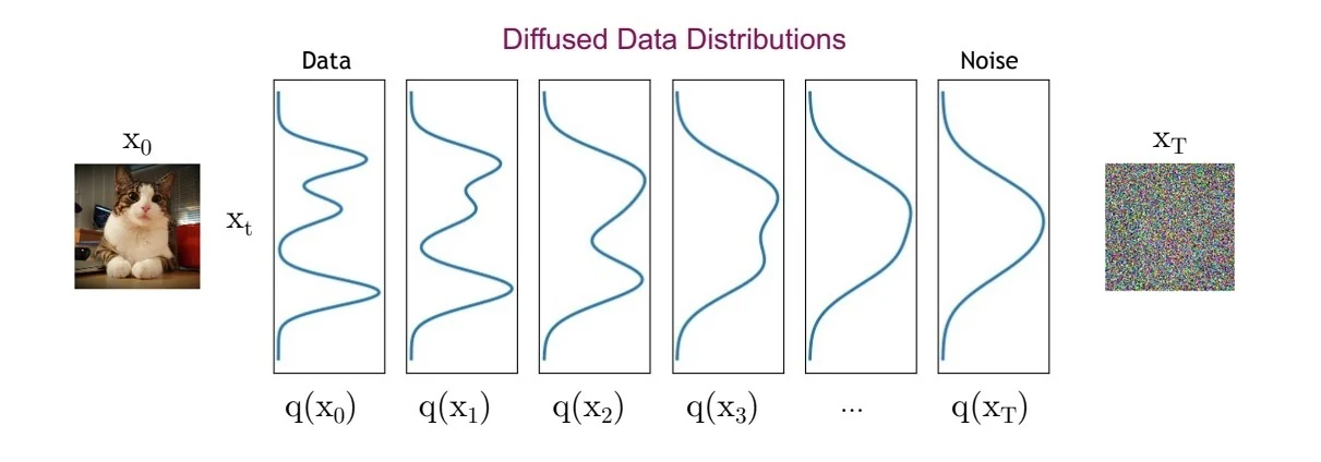
Figure 20.55: What happens to a distribution in the forward diffusion process? The forward noising process progressively transforms the original data distribution \( q(\mathbf {x}_0) \) into a standard Gaussian \( q(\mathbf {x}_T) \) through a sequence of small Gaussian perturbations. As the noise level increases, intermediate distributions \( q(\mathbf {x}_t) \) become increasingly blurred and entropic, eventually collapsing into an isotropic normal distribution. This transition enables generative modeling by allowing the use of a simple prior at sampling time. Source: Adapted from the CVPR 2022 diffusion models tutorial [604]. Trajectory Properties and Convergence While the step-by-step Gaussian transitions defined in Eq. 20.16 describe the local behavior of the diffusion process, understanding the global behavior of the entire trajectory \(\mathbf {x}_{0:T}\) is essential for both efficient training and theoretical justification.
The Joint Distribution and Markov Property The corruption process is explicitly designed as a Markov chain, meaning the probability of state \(\mathbf {x}_t\) depends solely on the immediate predecessor \(\mathbf {x}_{t-1}\) and not on the earlier history \(\mathbf {x}_{0:t-2}\). This conditional independence assumption allows the joint distribution of the entire forward trajectory to factorize cleanly into a product of local transitions: \begin {equation} \label {eq:chapter20_joint_distribution} q(\mathbf {x}_{1:T} \mid \mathbf {x}_0) = \prod _{t=1}^T q(\mathbf {x}_t \mid \mathbf {x}_{t-1}). \end {equation} This factorization is computationally advantageous: it implies that the complex transformation from data to noise is composed of simple, independent sampling steps, making the process analytically manageable.
Closed-Form Marginals: The ”Shortcut” Property A critical property of Gaussian diffusion is that we do not need to simulate the chain step-by-step to obtain a sample at an arbitrary timestep \(t\). Because the convolution of two Gaussians is another Gaussian, we can derive a closed-form expression for the marginal distribution \(q(\mathbf {x}_t \mid \mathbf {x}_0)\) directly. To simplify the notation, we define the signal retention schedules: \[ \alpha _t := 1 - \beta _t, \qquad \bar {\alpha }_t := \prod _{s=1}^t \alpha _s. \] Here, \(\bar {\alpha }_t\) represents the cumulative signal variance remaining after \(t\) steps. By recursively applying the reparameterization trick \(\mathbf {x}_t = \sqrt {\alpha _t}\mathbf {x}_{t-1} + \sqrt {1-\alpha _t}\boldsymbol {\epsilon }\), we can express \(\mathbf {x}_t\) as a linear combination of the original data \(\mathbf {x}_0\) and a merged noise term: \begin {equation} \label {eq:chapter20_marginal_closed_form} q(\mathbf {x}_t \mid \mathbf {x}_0) = \mathcal {N}\left (\mathbf {x}_t;\, \sqrt {\bar {\alpha }_t} \, \mathbf {x}_0,\, (1 - \bar {\alpha }_t) \mathbf {I} \right ). \end {equation} This identity is fundamental to the efficiency of diffusion models. It allows us to sample training data pairs \((\mathbf {x}_0, \mathbf {x}_t)\) instantly for any \(t\) without running the forward process loop, enabling highly efficient parallel training.
Asymptotic Convergence to Pure Noise The endpoint of the forward process is determined by the limit behavior of \(\bar {\alpha }_t\). For a properly chosen schedule where \(\sum \beta _t \to \infty \), the cumulative signal \(\bar {\alpha }_T\) approaches 0 as \(T \to \infty \). Consequently, the mean \(\sqrt {\bar {\alpha }_T}\mathbf {x}_0\) vanishes, and the variance \((1-\bar {\alpha }_T)\mathbf {I}\) approaches identity: \[ q(\mathbf {x}_T \mid \mathbf {x}_0) \approx \mathcal {N}(\mathbf {0}, \mathbf {I}). \] This convergence is theoretically grounded in two perspectives:
- 1.
- Central Limit Theorem (CLT): The final noise \(\mathbf {x}_T\) is effectively the sum of many independent, scaled noise injections from previous steps. Even if the local transitions were not perfectly Gaussian, the CLT suggests the cumulative result would tend toward a Gaussian distribution.
- 2.
- Ornstein–Uhlenbeck Process: The discrete steps can be viewed as a discretization of a continuous-time stochastic differential equation (SDE) known as the Ornstein–Uhlenbeck process, which is a mean-reverting process that converges to a stationary Gaussian distribution regardless of the starting state.
Practical Reality: The Finite Step Problem While the mathematical theory guarantees convergence to pure noise as \(T \to \infty \), practical engineering forces us to stop at a finite point (typically \(T=1000\)) to keep image generation times reasonable. This compromise creates a subtle but critical discrepancy known as Signal Leakage.
In standard diffusion algorithms (such as the baseline DDPM or the accelerated DDIM samplers we will cover later), the final cumulative noise schedule \(\bar {\alpha }_T\) is small but strictly non-zero.
- The ”Ghost” in the Noise: Consequently, the forward process does not reach perfect pure noise. The latent state \(\mathbf {x}_T\) effectively contains a “ghost” of the original data—usually faint, low-frequency structure that is imperceptible to the human eye but visible to a neural network.
- The Numerical Trap: Engineers explicitly avoid forcing \(\bar {\alpha }_T = 0\) (perfect noise) because the diffusion equations involve dividing by signal strength. As signal strength approaches zero, these terms approach infinity, causing numerical instability (exploding gradients) during training.
This safety measure creates a Training-Inference Mismatch. During training, the model learns to denoise \(\mathbf {x}_T\), subconsciously relying on that tiny ”ghost” signal to orient itself. However, during inference, we initialize the process from pure Gaussian noise \(\mathcal {N}(\mathbf {0}, \mathbf {I})\), which contains zero signal. The model, deprived of the hint it was trained to expect, often produces images with reduced contrast or a bias towards “medium gray” values.
The Modern Solution: Rectified Flow (RF) To solve this, state-of-the-art models are increasingly adopting Rectified Flow. While we will explore RF in depth in later chapters, the intuition is simple: Standard diffusion defines a distinct curve from data to noise that is mathematically difficult to define at the very end. RF reframes the problem as finding a straight line between data and noise. By predicting velocity (the rate of change) rather than noise, RF avoids the division-by-zero trap entirely. This allows the process to start at strictly perfect noise and end at strictly perfect data, eliminating the mismatch without requiring infinite steps.
Preparing for the Reverse Process Despite these modern evolutions, the vast majority of generative AI literature is built on the foundational diffusion framework. We proceed under the assumption that the corruption is effectively complete. The properties derived above—stable variance and closed-form marginals—define a corruption path that is mathematically invertible. By defining the forward process as a fixed, tractable Markov chain, we create a supervised learning setup: if we know the exact distribution \(q(\mathbf {x}_{t-1} \mid \mathbf {x}_t, \mathbf {x}_0)\), we can train a model to approximate it. This paves the path for the reverse process, where the model learns to synthesize realistic data by iteratively denoising pure Gaussian noise.
-
Reverse Process (Denoising, Generation)
The reverse (generative) process in diffusion models starts from pure Gaussian noise, \( \mathbf {x}_T \sim \mathcal {N}(\mathbf {0}, \mathbf {I}) \), and iteratively denoises it into a structured sample \(\mathbf {x}_0\) via a Markov chain: \begin {equation} \mathbf {x}_T \rightarrow \mathbf {x}_{T-1} \rightarrow \cdots \rightarrow \mathbf {x}_0. \label {eq:chapter20_reverse_chain} \end {equation} In an ideal world, each transition would sample from the true reverse conditional \(q(\mathbf {x}_{t-1}\mid \mathbf {x}_t)\). The core difficulty is that this unconditional reverse is not available in closed form for real data.
Why the True Reverse Step \( q(\mathbf {x}_{t-1} \mid \mathbf {x}_t) \) Is Intractable To generate data, we wish to sample from the reverse transition \( q(\mathbf {x}_{t-1} \mid \mathbf {x}_t) \). Let us attempt to derive this distribution analytically using Bayes’ rule. By definition: \begin {equation} \label {eq:chapter20_reverse_bayes} q(\mathbf {x}_{t-1} \mid \mathbf {x}_t) = \frac {q(\mathbf {x}_t \mid \mathbf {x}_{t-1}) \, q(\mathbf {x}_{t-1})}{q(\mathbf {x}_t)}. \end {equation} The first term in the numerator, \( q(\mathbf {x}_t \mid \mathbf {x}_{t-1}) \), is simply the forward diffusion kernel, which is a known Gaussian defined in Eq. 20.16.
However, the calculation breaks down when we examine the marginal probabilities \( q(\mathbf {x}_{t-1}) \) and \( q(\mathbf {x}_t) \). To compute the marginal density of a noisy sample \( \mathbf {x}_t \) , we must integrate over every possible clean image \( \mathbf {x}_0 \) that could have started the chain: \begin {equation} \label {eq:chapter20_marginal_integral} q(\mathbf {x}_t) = \int q(\mathbf {x}_t \mid \mathbf {x}_0) \, \underbrace {q(\mathbf {x}_0)}_{\mbox{Data dist.}} \, d\mathbf {x}_0. \end {equation} Here lies the fundamental problem:
- 1.
- Dependence on the Unknown Data Distribution: The term \( q(\mathbf {x}_0) \) represents the true underlying distribution of natural images (or the specific dataset). This distribution is highly complex, multimodal, and analytically unknown. We do not have a mathematical formula for ”the probability of a picture of a cat”.
- 2.
- Intractable Integration: Because we cannot write down \( q(\mathbf {x}_0) \) in closed form, we cannot perform the integration in Eq. 20.21. Consequently, we cannot calculate the normalization constant \( q(\mathbf {x}_t) \) required for Bayes’ rule.
Intuition: Asking ”What is the previous step given this noisy image?” is equivalent to asking ”Which clean image is this noisy blob most likely to have come from?”. Without knowing the distribution of clean images (the prior), we cannot distinguish between a ”likely” noisy version of a real object and a ”likely” noisy version of random static. Since evaluating the probability of every possible real-world image is impossible, the exact reverse step \( q(\mathbf {x}_{t-1} \mid \mathbf {x}_t) \) remains intractable.
A tractable “teacher” posterior during training During training, we observe the clean data sample \(\mathbf {x}_0 \sim p_{\mbox{data}}\) from the dataset. This distinction is critical: the unconditional reverse transition \(q(\mathbf {x}_{t-1}\mid \mathbf {x}_t)\) is intractable in the data setting because it marginalizes over the unknown data distribution. Concretely, by the law of total probability, \begin {equation} \label {eq:chapter20_intractable_reverse_as_mixture} q(\mathbf {x}_{t-1}\mid \mathbf {x}_t) = \int q(\mathbf {x}_{t-1}\mid \mathbf {x}_t,\mathbf {x}_0)\,q(\mathbf {x}_0\mid \mathbf {x}_t)\,d\mathbf {x}_0. \end {equation} Evaluating this integral would require the posterior \(q(\mathbf {x}_0\mid \mathbf {x}_t)\), which depends on the unknown prior \(p_{\mbox{data}}(\mathbf {x}_0)\) via Bayes’ rule: \(q(\mathbf {x}_0\mid \mathbf {x}_t) \propto q(\mathbf {x}_t\mid \mathbf {x}_0)p_{\mbox{data}}(\mathbf {x}_0)\).
However, if we condition on the specific ground-truth \(\mathbf {x}_0\) used to generate \(\mathbf {x}_t\) during training, the reverse posterior becomes fully analytic: \begin {equation} \label {eq:chapter20_teacher_posterior_def} q(\mathbf {x}_{t-1}\mid \mathbf {x}_t, \mathbf {x}_0). \end {equation} We will treat this tractable posterior as a teacher target: it is the “correct” denoising distribution (under the forward process assumptions) that a neural network (the student) should learn to approximate without access to \(\mathbf {x}_0\) at inference time.
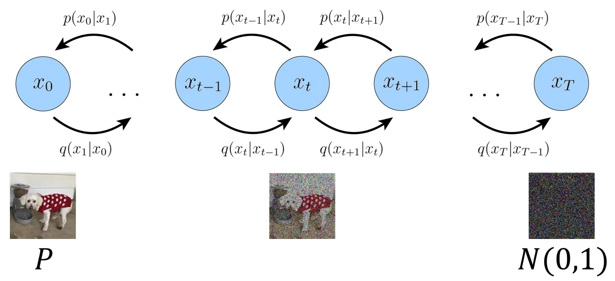
Figure 20.56: Visual intuition for the diffusion process. An input image is progressively corrupted with Gaussian noise over multiple steps (left to right), ultimately yielding pure noise. The learned denoising process (right to left) reverses this trajectory. Conditioning on \(\mathbf {x}_0\) makes the reverse-step posterior \(q(\mathbf {x}_{t-1}\mid \mathbf {x}_t,\mathbf {x}_0)\) a simple Gaussian with closed-form mean and variance, providing an exact training-time target. Adapted from [413]. Derivation of the Posterior \(q(\mathbf {x}_{t-1}\mid \mathbf {x}_t,\mathbf {x}_0)\) We assume the standard diffusion forward process following [232, 598]: \begin {equation} \label {eq:chapter20_forward_step} q(\mathbf {x}_t \mid \mathbf {x}_{t-1}) = \mathcal {N}\!\left (\mathbf {x}_t;\, \sqrt {\alpha _t}\,\mathbf {x}_{t-1},\, \beta _t \mathbf {I}\right ), \qquad \alpha _t := 1-\beta _t. \end {equation} Recall the closed-form marginal: \begin {equation} \label {eq:chapter20_forward_marginal_reparam_ref} q(\mathbf {x}_t\mid \mathbf {x}_0) = \mathcal {N}\!\left (\mathbf {x}_t;\, \sqrt {\bar {\alpha }_t}\,\mathbf {x}_0,\,(1-\bar {\alpha }_t)\mathbf {I}\right ), \qquad \bar {\alpha }_t = \prod _{s=1}^t \alpha _s. \end {equation}
Step 1: Bayes’ Rule and the Proportionality Argument
We aim to find the posterior distribution \( q(\mathbf {x}_{t-1} \mid \mathbf {x}_t, \mathbf {x}_0) \). Mathematically, we treat \( \mathbf {x}_{t-1} \) as the variable of interest, while \( \mathbf {x}_t \) and \( \mathbf {x}_0 \) are fixed observed values.
Using the definition of conditional probability, we expand the posterior: \begin {equation} \label {eq:chapter20_teacher_posterior_bayes_full} q(\mathbf {x}_{t-1} \mid \mathbf {x}_t, \mathbf {x}_0) = \frac {q(\mathbf {x}_t \mid \mathbf {x}_{t-1}, \mathbf {x}_0) \, q(\mathbf {x}_{t-1} \mid \mathbf {x}_0)}{q(\mathbf {x}_t \mid \mathbf {x}_0)}. \end {equation} First, we apply the Markov property to the first term in the numerator. Given the immediate past \( \mathbf {x}_{t-1} \), the future state \( \mathbf {x}_t \) depends only on the noise added at that step and is independent of the distant past \( \mathbf {x}_0 \). Thus, \( q(\mathbf {x}_t \mid \mathbf {x}_{t-1}, \mathbf {x}_0) \) simplifies to \( q(\mathbf {x}_t \mid \mathbf {x}_{t-1}) \).
Second, consider the denominator, \( q(\mathbf {x}_t \mid \mathbf {x}_0) \). Notice that this term depends only on \( \mathbf {x}_t \) and \( \mathbf {x}_0 \). Crucially, it does not contain the variable \( \mathbf {x}_{t-1} \). From the perspective of a function over \( \mathbf {x}_{t-1} \), the denominator is merely a constant scaling factor (often denoted as \( Z \) or \( C \)). In Gaussian derivation, it is standard practice to ignore such normalization constants and focus on the functional form (or kernel) of the distribution. If we can show that the exponent is quadratic in \( \mathbf {x}_{t-1} \), we define the distribution as Gaussian and calculate the normalization later (or infer it from the variance).
Therefore, we replace the equality with a proportionality sign (\( \propto \)), retaining only the terms that shape the distribution of \( \mathbf {x}_{t-1} \): \begin {equation} \label {eq:chapter20_posterior_product} q(\mathbf {x}_{t-1} \mid \mathbf {x}_t, \mathbf {x}_0) \propto \underbrace {q(\mathbf {x}_t \mid \mathbf {x}_{t-1})}_{\mbox{Likelihood (Forward Step)}} \cdot \underbrace {q(\mathbf {x}_{t-1} \mid \mathbf {x}_0)}_{\mbox{Prior (Marginal)}}. \end {equation}
Step 2: Analyzing the Gaussian Factors
We now define the explicit forms of these two factors using the forward process definitions.
1. The Prior Term (Marginal): This is the distribution of \( \mathbf {x}_{t-1} \) given the starting data \( \mathbf {x}_0 \). From the closed-form marginal property, we know: \begin {equation} \label {eq:chapter20_prior_xtm1_given_x0} q(\mathbf {x}_{t-1} \mid \mathbf {x}_0) = \mathcal {N}\left (\mathbf {x}_{t-1};\, \sqrt {\bar {\alpha }_{t-1}}\mathbf {x}_0,\; (1-\bar {\alpha }_{t-1})\mathbf {I}\right ), \end {equation} where \( \bar {\alpha }_{t-1} = \prod _{s=1}^{t-1} (1-\beta _s) \) is the cumulative signal variance.
2. The Likelihood Term (Transition): The forward transition is defined as a conditional distribution over the next step \( \mathbf {x}_t \): \[ q(\mathbf {x}_t \mid \mathbf {x}_{t-1}) = \mathcal {N}(\mathbf {x}_t; \sqrt {\alpha _t}\mathbf {x}_{t-1}, \beta _t\mathbf {I}), \quad \mbox{where } \alpha _t = 1 - \beta _t. \] To combine this with the prior (a distribution over \( \mathbf {x}_{t-1} \)), we need to multiply them. Since the prior is a function of \( \mathbf {x}_{t-1} \), it is mathematically convenient to also view this likelihood term as a function of \( \mathbf {x}_{t-1} \) (treating \( \mathbf {x}_t \) as a fixed observation).
Detailed Derivation: Inverting the Gaussian View Recall that the probability density function (PDF) of a Gaussian \( \mathcal {N}(\mathbf {y}; \boldsymbol {\mu }, \sigma ^2\mathbf {I}) \) is determined entirely by the term inside its exponent: \[ p(\mathbf {y}) \propto \exp \left ( -\frac {1}{2\sigma ^2} \|\mathbf {y} - \boldsymbol {\mu }\|^2 \right ). \] Any expression we can rearrange into the form \( \exp ( -\frac {1}{2C} \|\mathbf {x} - \mathbf {m}\|^2 ) \) implies a Gaussian distribution over \( \mathbf {x} \) with mean \( \mathbf {m} \) and variance \( C \).
Let us analyze the exponent of \( q(\mathbf {x}_t \mid \mathbf {x}_{t-1}) \): \[ E = -\frac {1}{2\beta _t} \|\mathbf {x}_t - \sqrt {\alpha _t}\mathbf {x}_{t-1}\|^2. \] Our goal is to isolate \( \mathbf {x}_{t-1} \) so that it looks like \( \|\mathbf {x}_{t-1} - \dots \|^2 \).
- 1.
- Symmetry of the Norm: The squared Euclidean distance is symmetric (\( \|a-b\|^2 = \|b-a\|^2 \)). We swap the terms to put our variable of interest, \( \mathbf {x}_{t-1} \), first: \[ \|\mathbf {x}_t - \sqrt {\alpha _t}\mathbf {x}_{t-1}\|^2 = \|\sqrt {\alpha _t}\mathbf {x}_{t-1} - \mathbf {x}_t\|^2. \]
- 2.
- Factoring out the Scalar: We want the coefficient of \( \mathbf {x}_{t-1} \) to be 1. We factor \( \sqrt {\alpha _t} \) out of the vector subtraction inside the norm: \[ \sqrt {\alpha _t}\mathbf {x}_{t-1} - \mathbf {x}_t = \sqrt {\alpha _t} \left ( \mathbf {x}_{t-1} - \frac {1}{\sqrt {\alpha _t}}\mathbf {x}_t \right ). \]
- 3.
- Squaring the Factor: Recall the norm property \( \|c \cdot \mathbf {v}\|^2 = c^2 \|\mathbf {v}\|^2 \). When we pull \( \sqrt {\alpha _t} \) outside the squared norm, it becomes \( (\sqrt {\alpha _t})^2 = \alpha _t \): \[ \left \| \sqrt {\alpha _t} \left ( \mathbf {x}_{t-1} - \frac {1}{\sqrt {\alpha _t}}\mathbf {x}_t \right ) \right \|^2 = \alpha _t \left \| \mathbf {x}_{t-1} - \frac {1}{\sqrt {\alpha _t}}\mathbf {x}_t \right \|^2. \]
- 4.
- Substituting Back: Now we plug this transformed norm back into the original exponential expression: \[ \exp (E) = \exp \left ( -\frac {1}{2\beta _t} \cdot \alpha _t \left \| \mathbf {x}_{t-1} - \frac {1}{\sqrt {\alpha _t}}\mathbf {x}_t \right \|^2 \right ). \]
- 5.
- Identifying Variance: We group the scalars to match the standard Gaussian form \( -\frac {1}{2\sigma ^2} \). \[ -\frac {\alpha _t}{2\beta _t} = -\frac {1}{2 (\beta _t / \alpha _t)}. \] This identifies the effective variance \( \sigma ^2 \) as \( \frac {\beta _t}{\alpha _t} \).
Conclusion: The functional form with respect to \( \mathbf {x}_{t-1} \) is: \[ \exp \left ( -\frac {1}{2 (\frac {\beta _t}{\alpha _t})} \left \| \mathbf {x}_{t-1} - \frac {1}{\sqrt {\alpha _t}}\mathbf {x}_t \right \|^2 \right ). \] By inspection, this is proportional to a Gaussian density with:
- Mean: \( \frac {1}{\sqrt {\alpha _t}}\mathbf {x}_t \) (the observed next step, scaled backwards).
- Variance: \( \frac {\beta _t}{\alpha _t}\mathbf {I} \) (the forward noise scaled by the inverse signal factor).
Thus, we write the proportionality: \begin {equation} \label {eq:chapter20_likelihood_as_gaussian_in_xtm1} q(\mathbf {x}_t \mid \mathbf {x}_{t-1}) \propto \mathcal {N}\left (\mathbf {x}_{t-1};\, \frac {1}{\sqrt {\alpha _t}}\mathbf {x}_t,\; \frac {\beta _t}{\alpha _t}\mathbf {I}\right ). \end {equation}
Step 3: Calculating Posterior Precision and Mean
We now multiply the two Gaussians derived above. The product of two Gaussians \( \mathcal {N}(\boldsymbol {\mu }_1, \boldsymbol {\Sigma }_1) \) and \( \mathcal {N}(\boldsymbol {\mu }_2, \boldsymbol {\Sigma }_2) \) is a new Gaussian \( \mathcal {N}(\tilde {\boldsymbol {\mu }}, \tilde {\boldsymbol {\Sigma }}) \), where the precisions (inverse variances) add: \begin {equation} \label {eq:chapter20_gaussian_product_identity} \tilde {\boldsymbol {\Sigma }}^{-1} = \boldsymbol {\Sigma }_1^{-1} + \boldsymbol {\Sigma }_2^{-1}, \qquad \tilde {\boldsymbol {\mu }} = \tilde {\boldsymbol {\Sigma }} \left ( \boldsymbol {\Sigma }_1^{-1}\boldsymbol {\mu }_1 + \boldsymbol {\Sigma }_2^{-1}\boldsymbol {\mu }_2 \right ). \end {equation} Substituting our specific variances \( \boldsymbol {\Sigma }_1 = \frac {\beta _t}{\alpha _t}\mathbf {I} \) and \( \boldsymbol {\Sigma }_2 = (1-\bar {\alpha }_{t-1})\mathbf {I} \):
\begin {equation} \label {eq:chapter20_posterior_precision_calc} \tilde {\beta }_t^{-1} \mathbf {I} = \left ( \frac {\alpha _t}{\beta _t} + \frac {1}{1-\bar {\alpha }_{t-1}} \right ) \mathbf {I} = \left ( \frac {\alpha _t(1-\bar {\alpha }_{t-1}) + \beta _t}{\beta _t(1-\bar {\alpha }_{t-1})} \right ) \mathbf {I}. \end {equation} Using the identity \( \bar {\alpha }_t = \alpha _t \bar {\alpha }_{t-1} \) and \( \beta _t = 1 - \alpha _t \), the numerator simplifies to \( 1 - \bar {\alpha }_t \). Inverting the result gives the closed-form posterior variance: \begin {equation} \label {eq:chapter20_posterior_variance} \tilde {\beta }_t = \frac {1-\bar {\alpha }_{t-1}}{1-\bar {\alpha }_t} \beta _t. \end {equation} Similarly, computing the weighted mean yields: \begin {equation} \label {eq:chapter20_posterior_mean_closedform} \tilde {\boldsymbol {\mu }}_t(\mathbf {x}_t, \mathbf {x}_0) = \frac {\sqrt {\bar {\alpha }_{t-1}}\beta _t}{1-\bar {\alpha }_t}\mathbf {x}_0 + \frac {\sqrt {\alpha _t}(1-\bar {\alpha }_{t-1})}{1-\bar {\alpha }_t}\mathbf {x}_t. \end {equation} This gives us the final tractable distribution \( q(\mathbf {x}_{t-1} \mid \mathbf {x}_t, \mathbf {x}_0) = \mathcal {N}(\tilde {\boldsymbol {\mu }}_t, \tilde {\beta }_t \mathbf {I}) \), which acts as the target for our neural network.
Reparameterizing the Posterior via Noise Prediction While the closed-form expression for the posterior mean \(\tilde {\boldsymbol {\mu }}_t(\mathbf {x}_t, \mathbf {x}_0)\) derived in Eq. (20.33) is mathematically exact, it presents a practical difficulty: it depends explicitly on the clean image \(\mathbf {x}_0\). At inference time, \(\mathbf {x}_0\) is exactly what we are trying to generate and is therefore unknown. To make this posterior useful for a generative model, we must re-express it in terms of quantities available to the network.
Recall the reparameterization of the forward marginal \(q(\mathbf {x}_t \mid \mathbf {x}_0)\), which relates the noisy state \(\mathbf {x}_t\) to the clean data \(\mathbf {x}_0\) and the cumulative noise \(\boldsymbol {\epsilon }\): \[ \mathbf {x}_t = \sqrt {\bar {\alpha }_t}\mathbf {x}_0 + \sqrt {1-\bar {\alpha }_t}\boldsymbol {\epsilon }, \quad \mbox{where } \boldsymbol {\epsilon } \sim \mathcal {N}(\mathbf {0}, \mathbf {I}). \] We can invert this relationship to express the unknown \(\mathbf {x}_0\) as a function of the current noisy state \(\mathbf {x}_t\) and the noise vector \(\boldsymbol {\epsilon }\): \[ \mathbf {x}_0 = \frac {\mathbf {x}_t - \sqrt {1-\bar {\alpha }_t}\boldsymbol {\epsilon }}{\sqrt {\bar {\alpha }_t}}. \] Substituting this expression back into the formula for the posterior mean \(\tilde {\boldsymbol {\mu }}_t\) (Eq. (20.33)) allows us to eliminate \(\mathbf {x}_0\). After algebraic simplification, we arrive at an implementation-critical identity that depends only on \(\mathbf {x}_t\) and \(\boldsymbol {\epsilon }\): \begin {equation} \label {eq:chapter20_posterior_mean_eps_form} \tilde {\boldsymbol {\mu }}_t(\mathbf {x}_t, \mathbf {x}_0) = \frac {1}{\sqrt {\alpha _t}} \left ( \mathbf {x}_t - \frac {\beta _t}{\sqrt {1-\bar {\alpha }_t}}\,\boldsymbol {\epsilon } \right ). \end {equation} Key Insight: This equation reveals that the optimal denoising step is just a scaled version of the input \(\mathbf {x}_t\) minus a scaled version of the noise \(\boldsymbol {\epsilon }\). Since \(\mathbf {x}_t\) is known at the current step, the only unknown quantity required to compute the optimal reverse trajectory is the noise \(\boldsymbol {\epsilon }\) itself. Therefore, learning to approximate the posterior mean is mathematically equivalent to learning to predict the noise present in the image.
Teacher–Student Learning: Matching the Posterior To perform generation, we introduce a learnable “student” model \(p_\theta \) designed to approximate the true time-reversed process. Since the true posterior \(q(\mathbf {x}_{t-1} \mid \mathbf {x}_t, \mathbf {x}_0)\) is Gaussian, we parameterize the student transition also as a Gaussian: \begin {equation} \label {eq:chapter20_student_reverse_gaussian} p_\theta (\mathbf {x}_{t-1} \mid \mathbf {x}_t) = \mathcal {N}\!\left (\mathbf {x}_{t-1};\,\boldsymbol {\mu }_\theta (\mathbf {x}_t,t),\,\sigma _t^2\mathbf {I}\right ). \end {equation} Here, \(\boldsymbol {\mu }_\theta \) is a neural network (typically a U-Net) that predicts the mean of the next state, and \(\sigma _t^2\) is the variance (often set to a fixed schedule such as \(\beta _t\) or \(\tilde {\beta }_t\)).
We train this model using a Teacher–Student framework. During training, we have access to the ground truth data, so the exact posterior \(q(\mathbf {x}_{t-1} \mid \mathbf {x}_t, \mathbf {x}_0)\) (the “teacher”) is computable. We optimize the student parameters \(\theta \) to match the teacher by minimizing the Kullback-Leibler (KL) divergence at every timestep: \begin {equation} \label {eq:chapter20_teacher_student_kl} \mathcal {L}_t(\theta ) = \mathrm {KL}\!\left ( q(\mathbf {x}_{t-1}\mid \mathbf {x}_t,\mathbf {x}_0) \;\|\; p_\theta (\mathbf {x}_{t-1}\mid \mathbf {x}_t) \right ). \end {equation} Because the KL divergence between two Gaussians is dominated by the squared Euclidean distance between their means, minimizing this objective is equivalent (up to scaling factors) to minimizing the Mean Squared Error (MSE) between the teacher’s mean \(\tilde {\boldsymbol {\mu }}_t\) and the student’s predicted mean \(\boldsymbol {\mu }_\theta \).
The Noise-Prediction Objective Leveraging the insight from Eq. (20.34), we parameterize the student network not to predict the mean directly, but to predict the noise \(\boldsymbol {\epsilon }\). We define the network output \(\boldsymbol {\epsilon }_\theta (\mathbf {x}_t, t)\) and construct the mean prediction as: \begin {equation} \label {eq:chapter20_mu_theta_from_eps} \boldsymbol {\mu }_\theta (\mathbf {x}_t,t) := \frac {1}{\sqrt {\alpha _t}} \left ( \mathbf {x}_t - \frac {\beta _t}{\sqrt {1-\bar {\alpha }_t}}\,\boldsymbol {\epsilon }_\theta (\mathbf {x}_t,t) \right ). \end {equation} By substituting this parameterization into the KL divergence objective, the loss function simplifies significantly. The complicated coefficients describing the mean collapse into a single time-dependent weight, and the target becomes simply the true noise vector \(\boldsymbol {\epsilon }\) sampled during the forward process: \begin {equation} \label {eq:chapter20_eps_mse_weighted} \mathcal {L}_t(\theta ) = \mathbb {E}_{\mathbf {x}_0,\boldsymbol {\epsilon }}\!\left [ \lambda _t \;\big \|\boldsymbol {\epsilon } - \boldsymbol {\epsilon }_\theta (\mathbf {x}_t, t)\big \|_2^2 \right ], \quad \mbox{where } \lambda _t = \frac {\beta _t^2}{2\sigma _t^2 \alpha _t (1-\bar {\alpha }_t)}. \end {equation} This result is profound: complex generative modeling is reduced to a sequence of denoising autoencoder tasks. The network simply learns to look at a noisy image \(\mathbf {x}_t\) and estimate the noise \(\boldsymbol {\epsilon }\) that corrupted it.
Theoretical Justification: The Variational Lower Bound (ELBO) One might ask: is matching the posterior at each step strictly equivalent to maximizing the likelihood of the generated data? The answer is yes, provided we consider the entire trajectory.
The local teacher–student objectives \(\mathcal {L}_t\) arise naturally from maximizing the Evidence Lower Bound (ELBO) on the log-likelihood \(\log p_\theta (\mathbf {x}_0)\). Just as in VAEs, where we optimize a bound on the marginal likelihood of the data, diffusion models optimize a bound derived from the joint distribution of the forward and reverse chains: \begin {equation} \label {eq:chapter20_elbo_decomposition_general} \log p_\theta (\mathbf {x}_0) \ge \mathcal {L}_{\mathrm {ELBO}} = \mathbb {E}_{q}\left [ \log \frac {p_\theta (\mathbf {x}_{0:T})}{q(\mathbf {x}_{1:T} \mid \mathbf {x}_0)} \right ]. \end {equation} When expanded, this global objective decomposes into a sum of local terms corresponding exactly to the objectives we derived heuristically: \begin {equation} \label {eq:chapter20_elbo_decomposition_explicit} \mathcal {L}_{\mathrm {ELBO}} = \underbrace {-\,\mathrm {KL}(q(\mathbf {x}_T|\mathbf {x}_0)\,\|\,p(\mathbf {x}_T))}_{\mbox{Prior Matching}} \;-\; \sum _{t=2}^T \underbrace {\mathbb {E}_{q}\!\left [\mathrm {KL}(q(\mathbf {x}_{t-1}|\mathbf {x}_t,\mathbf {x}_0)\,\|\,p_\theta (\mathbf {x}_{t-1}|\mathbf {x}_t))\right ]}_{\mbox{Denoising Matching (Teacher-Student)}} \;+\; \underbrace {\mathbb {E}_{q}\!\left [\log p_\theta (\mathbf {x}_0|\mathbf {x}_1)\right ]}_{\mbox{Reconstruction}}. \end {equation} This decomposition proves that by training the model to match the teacher posterior (denoising matching) and ensuring the final latent matches the prior (prior matching), we are mathematically maximizing the likelihood of the generated data.
In the following section, we will explore the specific algorithm that instantiates this framework—the Denoising Diffusion Probabilistic Model (DDPM)—and detail the practical simplifications, such as discarding the weighting term \(\lambda _t\), that lead to a practical diffusion approach for image generation.
Enrichment 20.9.2: Denoising Diffusion Probabilistic Models (DDPM)
Denoising Diffusion Probabilistic Models (DDPM) [232] represent a seminal advance in the development of practical and highly effective diffusion-based generative models. DDPMs distill the general diffusion modeling framework into a concrete, efficient, and empirically powerful algorithm for image synthesis—transforming the theoretical appeal of diffusion into state-of-the-art results on real data.
Enrichment 20.9.2.1: Summary of Core Variables in Diffusion Models
Purpose and Motivation Before deriving the ELBO-based training objective of DDPMs, it is critical to clearly understand the set of variables and coefficients that structure both the forward and reverse processes. The loss function ultimately minimized in DDPMs is derived from the KL divergence between a true posterior and a learned reverse process. Both of these distributions depend intimately on Gaussian means and variances computed using scalar quantities such as \( \beta _t \), \( \alpha _t \), \( \bar {\alpha }_t \), and \( \tilde {\beta }_t \). Without explicitly recalling what these mean—and how they interact—the derivation of the objective risks becoming opaque or unmotivated.
Practical Implementation: Reverse Variance and Sampling While the mean \(\boldsymbol {\mu }_\theta (\mathbf {x}_t, t)\) is learned via the noise prediction objective, the reverse process variance \(\sigma _t^2\) must also be defined to perform sampling.
1. Choices for Reverse Variance \( \sigma _t^2 \) The full reverse transition is
\( p_\theta (\mathbf {x}_{t-1} \mid \mathbf {x}_t) = \mathcal {N}(\mathbf {x}_{t-1};\, \boldsymbol {\mu }_\theta (\mathbf {x}_t, t),\, \sigma _t^2 \mathbf {I}) \). Two common strategies exist for setting \(\sigma _t^2\):
- Posterior-matching (\( \sigma _t^2 = \tilde {\beta }_t \)): Sets the variance to the true posterior variance derived in Eq. (20.32). This aligns the model with the theoretical reverse process and is analytically precise.
- Forward-matching (\( \sigma _t^2 = \beta _t \)): Sets the variance to the forward noise schedule. This is often empirically stable and simpler to implement. Ideally, \(\tilde {\beta }_t \approx \beta _t\) when sampling steps are small, making them interchangeable in practice [232].
2. The Role of Stochasticity (Why Inject Noise?) The sampling update rule is: \[ \mathbf {x}_{t-1} = \boldsymbol {\mu }_\theta (\mathbf {x}_t, t) + \sigma _t \mathbf {z}, \quad \mbox{where } \mathbf {z} \sim \mathcal {N}(\mathbf {0}, \mathbf {I}). \] Why do we add the random noise term \(\sigma _t \mathbf {z}\) instead of just taking the predicted mean?
- Generative Diversity: The noise injection ensures the process remains stochastic. It allows the model to generate multiple distinct outputs \(\mathbf {x}_0\) from the same starting noise \(\mathbf {x}_T\), exploring the full diversity of the data distribution.
- Correcting Errors: Without noise, the process would collapse into a deterministic trajectory that might drift off the data manifold. The noise corrects small errors in the mean prediction, keeping the trajectory “fuzzy” enough to land in a valid high-probability region.
Note: In the final step (\(t=1\)), noise is typically omitted (\(\mathbf {z}=\mathbf {0}\)) to output the best clean estimate without adding residual grain.
Intuitive Summary of Core Variables To navigate the derivation and implementation of diffusion models, it is essential to build a strong intuition for the four scalar schedules and tensor quantities that govern the process. We summarize them here as functional components of the generative engine:
- The Corruption Schedule (\( \beta _t \)): Controls the rate of information destruction. A small \( \beta _t \) implies a gentle diffusion step where image structure is preserved, whereas a large \( \beta _t \) represents aggressive corruption. The schedule \( \{ \beta _t \}_{t=1}^T \) is monotonically increasing to ensure data is slowly dissolved into noise rather than destroyed abruptly [232].
- Cumulative Signal Health (\( \bar {\alpha }_t \)): Quantifies the remaining signal strength of \( \mathbf {x}_0 \) inside the noisy state \( \mathbf {x}_t \). Defined as \( \prod _{s=1}^t (1-\beta _s) \), it acts as a “signal-to-noise” ratio indicator. When \( \bar {\alpha }_t \approx 1 \) (early \( t \)), the sample is pristine; when \( \bar {\alpha }_t \to 0 \) (late \( t \)), the sample is effectively pure Gaussian noise. This scalar allows us to jump directly to any timestep during training without simulating intermediate steps.
- The Ideal Reverse Target (\( \tilde {\boldsymbol {\mu }}_t \)): Represents the optimal denoising destination. If we had access to the ground truth \( \mathbf {x}_0 \), \( \tilde {\boldsymbol {\mu }}_t \) is exactly where we should move \( \mathbf {x}_t \) to optimally reverse the last noise injection. It is a weighted blend of the noisy observation (what we see) and the clean signal (what we know). Training essentially forces the model to guess this target without seeing \( \mathbf {x}_0 \).
- The Learned Gradient (\( \boldsymbol {\epsilon }_\theta \)): The engine of generation. Instead of predicting the image directly, the network estimates the noise vector pointing “away” from the data manifold. Subtracting this estimated noise from \( \mathbf {x}_t \) (scaled appropriately) pushes the sample effectively “towards” the clean data distribution, approximating the score function (gradient of the log-density).
Enrichment 20.9.2.2: ELBO Formulation and Loss Decomposition
Maximum Likelihood with a Latent Diffusion Trajectory A DDPM functions as a latent-variable generative model, but with a distinct structure: its latent variables are the sequence of intermediate noisy states \(\mathbf {x}_{1:T}\) rather than a single compressed vector. Notably, each latent \(\mathbf {x}_t \in \mathbb {R}^D\) maintains the same dimensionality as the input data \(\mathbf {x}_0 \in \mathbb {R}^D\).
The generative process is defined as a reverse Markov chain that
begins with pure noise \(\mathbf {x}_T\) and progressively removes it to synthesize data: \begin {equation} \label {eq:chapter20_reverse_chain_joint} p_\theta (\mathbf {x}_{0:T}) = p(\mathbf {x}_T)\prod _{t=1}^{T} p_\theta (\mathbf {x}_{t-1}\mid \mathbf {x}_t), \qquad p(\mathbf {x}_T)=\mathcal {N}(\mathbf {0},\mathbf {I}). \end {equation}
Here, each transition \(p_\theta (\mathbf {x}_{t-1}\mid \mathbf {x}_t)\) is typically modeled as a time-conditional Gaussian
\( \mathcal {N}(\mathbf {x}_{t-1}; \boldsymbol {\mu }_\theta (\mathbf {x}_t, t), \boldsymbol {\Sigma }_\theta (t)) \), where the mean is parameterized by a neural network.
Training this model by maximum likelihood requires optimizing the marginal log-likelihood of the observed data \(\mathbf {x}_0\): \begin {equation} \label {eq:chapter20_marginal_likelihood_integral} \log p_\theta (\mathbf {x}_0) = \log \int p_\theta (\mathbf {x}_{0:T})\, d\mathbf {x}_{1:T}. \end {equation} This integral necessitates marginalizing over all possible high-dimensional trajectories \(\mathbf {x}_{1:T}\) that could have collapsed into \(\mathbf {x}_0\). Due to the depth of the chain (\(T \approx 1000\)) and the complex, learned nature of the reverse transitions, this computation is analytically intractable.
Introducing the Forward Process as a Variational Distribution To obtain a tractable objective, we introduce an auxiliary distribution \(q(\mathbf {x}_{1:T}\mid \mathbf {x}_0)\) and apply variational inference. In diffusion models, the key design choice is to set \(q\) to the fixed forward noising process [232, 598]: \begin {equation} \label {eq:chapter20_forward_chain} q(\mathbf {x}_{1:T}\mid \mathbf {x}_0)=\prod _{t=1}^T q(\mathbf {x}_t\mid \mathbf {x}_{t-1}), \qquad q(\mathbf {x}_t\mid \mathbf {x}_{t-1}) = \mathcal {N}\!\left (\mathbf {x}_t;\sqrt {\alpha _t}\mathbf {x}_{t-1},\beta _t\mathbf {I}\right ). \end {equation} This distribution is defined by a fixed noise schedule \(\beta _t\in (0,1)\) and \(\alpha _t:=1-\beta _t\). Because each transition is Gaussian, \(q(\mathbf {x}_{1:T}\mid \mathbf {x}_0)\) spans the entire space \(\mathbb {R}^{DT}\), ensuring that the log-ratios in the objective are well-defined for any possible trajectory.
From the “Missing Integral” to a Tractable Expectation To make the marginal likelihood \( \log p_\theta (\mathbf {x}_0) \) computable, we transform the integration problem into an expectation problem. We multiply and divide the term inside the integral by our chosen variational distribution \(q(\mathbf {x}_{1:T}\mid \mathbf {x}_0)\): \begin {align} \log p_\theta (\mathbf {x}_0) &= \log \int q(\mathbf {x}_{1:T}\mid \mathbf {x}_0)\, \frac {p_\theta (\mathbf {x}_{0:T})}{q(\mathbf {x}_{1:T}\mid \mathbf {x}_0)}\, d\mathbf {x}_{1:T} \label {eq:chapter20_importance_identity}\\ &= \log \mathbb {E}_{q(\mathbf {x}_{1:T}\mid \mathbf {x}_0)} \left [ \frac {p_\theta (\mathbf {x}_{0:T})}{q(\mathbf {x}_{1:T}\mid \mathbf {x}_0)} \right ]. \label {eq:chapter20_expectation_form} \end {align}
Why is this transformation useful? The move from Eq. (20.21) to Eq. (20.21) leverages the definition of the expected value: \(\mathbb {E}_q[f(\mathbf {x})] \equiv \int q(\mathbf {x})f(\mathbf {x}) d\mathbf {x}\). While the original integral requires evaluating all possible noise trajectories (an infinite and intractable set), the expectation form allows us to use Monte Carlo estimation.
Instead of analytically solving the integral, we can approximate the expectation by sampling a single trajectory \(\mathbf {x}_{1:T}\) from the forward process \(q\). Since \(q\) is a fixed Gaussian Markov chain, generating these samples is computationally trivial. This transforms the problem from impossible high-dimensional integration to simple stochastic sampling.
Jensen’s Inequality and the ELBO Because \(\log \) is concave, Jensen’s inequality (\(\log \mathbb {E}[X] \ge \mathbb {E}[\log X]\)) gives a lower bound: \begin {align} \log p_\theta (\mathbf {x}_0) &\ge \mathbb {E}_{q(\mathbf {x}_{1:T}\mid \mathbf {x}_0)} \left [ \log \frac {p_\theta (\mathbf {x}_{0:T})}{q(\mathbf {x}_{1:T}\mid \mathbf {x}_0)} \right ] =: \mathcal {L}_{\mathrm {ELBO}}(\theta ;\mathbf {x}_0). \label {eq:chapter20_elbo_definition} \end {align}
Maximizing \(\mathcal {L}_{\mathrm {ELBO}}\) is therefore a principled surrogate for maximizing \(\log p_\theta (\mathbf {x}_0)\).
Expanding the ELBO: Products Become Sums Substituting the Markov factorizations from Eqs. (20.41)–(20.43) into Eq. (20.41) and using \(\log \prod _t a_t=\sum _t\log a_t\) yields \begin {align} \mathcal {L}_{\mathrm {ELBO}}(\theta ;\mathbf {x}_0) = \mathbb {E}_{q} \Big [ \log p(\mathbf {x}_T) + \sum _{t=1}^{T}\log p_\theta (\mathbf {x}_{t-1}\mid \mathbf {x}_t) - \sum _{t=1}^{T}\log q(\mathbf {x}_t\mid \mathbf {x}_{t-1}) \Big ], \label {eq:chapter20_elbo_expanded_raw} \end {align}
where \(q\) is shorthand for \(q(\mathbf {x}_{1:T}\mid \mathbf {x}_0)\). This form is correct but not yet aligned with the backward-time conditionals that will appear in KL divergences.
The Posterior Trick: Aligning the Forward and Reverse Directions We face a structural mismatch in the ELBO derived so far (Eq. (20.124)). The ELBO contains a sum of forward transitions \(\log q(\mathbf {x}_t \mid \mathbf {x}_{t-1})\), which describe the diffusion process going forward in time. However, our generative model \(p_\theta (\mathbf {x}_{t-1} \mid \mathbf {x}_t)\) operates backward in time. To define a meaningful loss function (like a KL divergence), we must compare distributions that define the same transition direction (\(t \to t-1\)).
To fix this, we do not ”solve” for an unknown; rather, we use Bayes’ rule to rewrite the forward term \(\log q(\mathbf {x}_t \mid \mathbf {x}_{t-1})\) into an equivalent expression involving the reverse posterior.
1. Inverting the arrow with Bayes’ Rule
Recall that for the Markov chain conditioned on \(\mathbf {x}_0\), the reverse posterior is defined
as: \[ q(\mathbf {x}_{t-1} \mid \mathbf {x}_t, \mathbf {x}_0) = \frac {q(\mathbf {x}_t \mid \mathbf {x}_{t-1}, \mathbf {x}_0) \, q(\mathbf {x}_{t-1} \mid \mathbf {x}_0)}{q(\mathbf {x}_t \mid \mathbf {x}_0)}. \] Using the Markov property \(q(\mathbf {x}_t \mid \mathbf {x}_{t-1}, \mathbf {x}_0) = q(\mathbf {x}_t \mid \mathbf {x}_{t-1})\), we can rearrange this identity to isolate the
forward term found in our ELBO: \begin {equation} \label {eq:chapter20_bayes_identity_telescoping} \log q(\mathbf {x}_t \mid \mathbf {x}_{t-1}) = \underbrace {\log q(\mathbf {x}_{t-1} \mid \mathbf {x}_t, \mathbf {x}_0)}_{\mbox{Aligned Reverse Posterior}} + \underbrace {\log q(\mathbf {x}_t \mid \mathbf {x}_0) - \log q(\mathbf {x}_{t-1} \mid \mathbf {x}_0)}_{\mbox{Normalization Constants}}. \end {equation} Why do this? We have successfully replaced
a term pointing ”forward” (which we cannot compare to \(p_\theta \)) with a term
pointing ”backward” (which we can compare to \(p_\theta \)) plus some residual
marginals.
2. The Telescoping Sum
When we sum this substitution over all timesteps \(t=2 \dots T\), the residual marginal terms
cancel each other out in a cascading (telescoping) series: \begin {align} \sum _{t=2}^{T} \left [ \log q(\mathbf {x}_t|\mathbf {x}_0) - \log q(\mathbf {x}_{t-1}|\mathbf {x}_0) \right ] &= (\log q(\mathbf {x}_2|\mathbf {x}_0) - \log q(\mathbf {x}_1|\mathbf {x}_0)) \nonumber \\ &\quad + (\log q(\mathbf {x}_3|\mathbf {x}_0) - \log q(\mathbf {x}_2|\mathbf {x}_0)) \nonumber \\ &\quad + \dots \nonumber \\ &\quad + (\log q(\mathbf {x}_T|\mathbf {x}_0) - \log q(\mathbf {x}_{T-1}|\mathbf {x}_0)) \nonumber \\ &= \log q(\mathbf {x}_T \mid \mathbf {x}_0) - \log q(\mathbf {x}_1 \mid \mathbf {x}_0). \label {eq:chapter20_telescoping_cancellation} \end {align}
This effectively removes all intermediate marginals from the loss function. When we combine this result with the \(t=1\) term from the original sum, the final expression simplifies to just the sum of reverse posteriors plus the endpoint at \(T\): \begin {equation} \label {eq:chapter20_forward_sum_rewritten} \sum _{t=1}^{T} \log q(\mathbf {x}_t \mid \mathbf {x}_{t-1}) = \sum _{t=2}^{T} \log q(\mathbf {x}_{t-1} \mid \mathbf {x}_t, \mathbf {x}_0) + \log q(\mathbf {x}_T \mid \mathbf {x}_0). \end {equation}
ELBO Decomposition into the Standard DDPM Terms We now consolidate the terms to reveal the final objective. Recall our starting point: the expanded ELBO from Eq. (20.1). \[ \mathcal {L}_{\mathrm {ELBO}} = \mathbb {E}_{q(\mathbf {x}_{1:T} \mid \mathbf {x}_0)} \Bigg [ \log p(\mathbf {x}_T) + \sum _{t=1}^T \log p_\theta (\mathbf {x}_{t-1} \mid \mathbf {x}_t) - \sum _{t=1}^T \log q(\mathbf {x}_t \mid \mathbf {x}_{t-1}) \Bigg ]. \]
The Obstacle (Direction Mismatch): We want to train the reverse model \( p_\theta (\mathbf {x}_{t-1} \mid \mathbf {x}_t) \). Ideally, we would minimize a distance (like KL divergence) between this model and some ground truth. However, the ELBO currently contains the forward terms \( \log q(\mathbf {x}_t \mid \mathbf {x}_{t-1}) \). These point in the wrong direction (time \( t-1 \to t \)). We cannot directly compare a forward transition \( q \) to a reverse transition \( p_\theta \). To fix this, we must replace the forward sum with terms that point backwards in time.
Step 1: Applying the Telescoping Substitution
We substitute the forward sum using the telescoping identity derived in
Eq. (20.45): \[ \sum _{t=1}^{T} \log q(\mathbf {x}_t \mid \mathbf {x}_{t-1}) = \log q(\mathbf {x}_T \mid \mathbf {x}_0) + \sum _{t=2}^{T} \log q(\mathbf {x}_{t-1} \mid \mathbf {x}_t, \mathbf {x}_0). \] Notice that the terms inside the sum, \( q(\mathbf {x}_{t-1} \mid \mathbf {x}_t, \mathbf {x}_0) \), now point backwards
(from \( t \) to \( t-1 \)), conditioned on \( \mathbf {x}_0 \). This aligns perfectly with our generative model
\( p_\theta (\mathbf {x}_{t-1} \mid \mathbf {x}_t) \).
Step 2: Regrouping the ELBO
Substituting this back into the ELBO and grouping matching terms (prior with
prior, transition with transition): \begin {align} \mathcal {L}_{\mathrm {ELBO}} = \mathbb {E}_{q(\mathbf {x}_{1:T} \mid \mathbf {x}_0)} \Bigg [ &\underbrace {\log p_\theta (\mathbf {x}_0 \mid \mathbf {x}_1)}_{\text {Reconstruction } (t=1)} \nonumber \\ + &\underbrace {\left ( \log p(\mathbf {x}_T) - \log q(\mathbf {x}_T \mid \mathbf {x}_0) \right )}_{\text {Prior Matching } (t=T)} \nonumber \\ + &\sum _{t=2}^{T} \underbrace {\left ( \log p_\theta (\mathbf {x}_{t-1} \mid \mathbf {x}_t) - \log q(\mathbf {x}_{t-1} \mid \mathbf {x}_t, \mathbf {x}_0) \right )}_{\text {Denoising Matching } (t=2 \dots T)} \Bigg ]. \end {align}
Step 3: From Global Expectation to Local KLs
The expectation \( \mathbb {E}_{q(\mathbf {x}_{1:T} \mid \mathbf {x}_0)} \) is an integral over the entire trajectory. However, each grouped
term depends on only a few variables. We can simplify the expectations by
marginalizing out the irrelevant variables.
- Prior Term: Depends only on \( \mathbf {x}_T \). \[ \mathbb {E}_{q(\mathbf {x}_{1:T} \mid \mathbf {x}_0)} \left [ \log \frac {p(\mathbf {x}_T)}{q(\mathbf {x}_T \mid \mathbf {x}_0)} \right ] = \mathbb {E}_{q(\mathbf {x}_T \mid \mathbf {x}_0)} \left [ \log \frac {p(\mathbf {x}_T)}{q(\mathbf {x}_T \mid \mathbf {x}_0)} \right ] = -\mathrm {KL}(q(\mathbf {x}_T \mid \mathbf {x}_0) \,\|\, p(\mathbf {x}_T)). \]
- Denoising Terms (\(t>1\)): The term at step \( t \) depends on \( \mathbf {x}_t \) and \( \mathbf {x}_{t-1} \). We can split the expectation using the chain rule \( q(\mathbf {x}_t, \mathbf {x}_{t-1} \mid \mathbf {x}_0) = q(\mathbf {x}_{t-1} \mid \mathbf {x}_t, \mathbf {x}_0) q(\mathbf {x}_t \mid \mathbf {x}_0) \): \[ \mathbb {E}_{q(\mathbf {x}_{1:T} \mid \mathbf {x}_0)} \left [ \dots \right ] = \mathbb {E}_{q(\mathbf {x}_t \mid \mathbf {x}_0)} \Bigg [ \underbrace {\mathbb {E}_{q(\mathbf {x}_{t-1} \mid \mathbf {x}_t, \mathbf {x}_0)} \left [ \log \frac {p_\theta (\mathbf {x}_{t-1} \mid \mathbf {x}_t)}{q(\mathbf {x}_{t-1} \mid \mathbf {x}_t, \mathbf {x}_0)} \right ]}_{-\mathrm {KL}(q(\mathbf {x}_{t-1} \mid \mathbf {x}_t, \mathbf {x}_0) \,\|\, p_\theta (\mathbf {x}_{t-1} \mid \mathbf {x}_t))} \Bigg ]. \] The inner expectation is exactly the negative KL divergence between the posterior and the model. The outer expectation averages this KL over all possible noise levels \( \mathbf {x}_t \) sampled from \( q(\mathbf {x}_t \mid \mathbf {x}_0) \).
The Standard Variational Bound Decomposition We customarily minimize the negative ELBO (denoted \( L \)). Combining the results above yields the canonical decomposition from the DDPM paper [232]: \begin {equation} \label {eq:chapter20_vlb_decomp_L_terms} L = \underbrace {L_0}_{\mbox{Reconstruction}} + \underbrace {L_T}_{\mbox{Prior Matching}} + \sum _{t=2}^{T} \underbrace {L_{t-1}}_{\mbox{Denoising Matching}}, \end {equation} where the individual loss terms are defined as: \begin {align} L_0 &:= -\log p_\theta (\mathbf {x}_0 \mid \mathbf {x}_1), \label {eq:chapter20_L0_def}\\ L_T &:= \mathrm {KL}(q(\mathbf {x}_T \mid \mathbf {x}_0) \,\|\, p(\mathbf {x}_T)), \label {eq:chapter20_LT_def}\\ L_{t-1} &:= \mathbb {E}_{q(\mathbf {x}_t \mid \mathbf {x}_0)} \Big [ \mathrm {KL}(q(\mathbf {x}_{t-1} \mid \mathbf {x}_t, \mathbf {x}_0) \,\|\, p_\theta (\mathbf {x}_{t-1} \mid \mathbf {x}_t)) \Big ]. \label {eq:chapter20_Lt_def} \end {align}
Why is this powerful? Because we chose Gaussian transitions for both the forward process \( q \) and the reverse model \( p_\theta \), every KL divergence inside \( L_T \) and \( L_{t-1} \) can be computed in closed form. This avoids high-variance Monte Carlo estimates for the KL terms themselves. We only need to sample the outer expectation \( \mathbb {E}_{q(\mathbf {x}_t \mid \mathbf {x}_0)} \), which is efficiently handled by sampling a single \( \mathbf {x}_t \) during each training step.
Interpretation: What Each Term Is Doing (and What Actually Trains \(\theta \)) Eq. (20.46) isolates exactly where learning happens:
- Stepwise denoising KLs \(\mathcal {L}_{t-1}\) (the main trainable supervision). For each \(t\ge 2\), the model transition \(p_\theta (\mathbf {x}_{t-1}\mid \mathbf {x}_t)\) is trained to match the true posterior \(q(\mathbf {x}_{t-1}\mid \mathbf {x}_t,\mathbf {x}_0)\) induced by the forward process. This is the core “analytic teacher / learned student” mechanism: during training \(\mathbf {x}_0\) is known, so the teacher posterior is tractable; at sampling time \(\mathbf {x}_0\) is unknown, so only \(p_\theta \) remains.
- Prior KL \(\mathcal {L}_T\) (typically \(\theta \)-independent). With a fixed forward schedule and fixed prior \(p(\mathbf {x}_T)\), \(\mathcal {L}_T\) depends only on \(q\) and \(p\), and contributes no gradient to \(\theta \). Conceptually, it accounts for matching the endpoint distribution of the forward chain to the chosen prior.
- Decoder / reconstruction \(\mathcal {L}_0\). This term trains the final step mapping a lightly noised \(\mathbf {x}_1\) back to data \(\mathbf {x}_0\). It plays the same role as a VAE decoder likelihood term: its exact form is an implementation choice (e.g., a discretized Gaussian when \(\mathbf {x}_0\) is integer-valued pixel data).
Why This Matters for Implementation This decomposition is not a heuristic: it is the variational identity that converts an intractable marginal likelihood objective into a sum of tractable per-timestep losses. In practice, we estimate these expectations by sampling a minibatch \(\mathbf {x}_0\), drawing a timestep \(t\), sampling \(\mathbf {x}_t\sim q(\mathbf {x}_t\mid \mathbf {x}_0)\), and evaluating the corresponding term. Once we choose a parameterization of the reverse Gaussian mean (e.g., predicting \(\boldsymbol {\epsilon }\) or \(\mathbf {x}_0\)), the denoising KLs \(\mathcal {L}_{t-1}\) reduce (up to \(\theta \)-independent constants and known timestep-dependent weights) to the simple regression objectives used in modern implementations [232, 463].
Enrichment 20.9.2.3: Training and Inference in DDPMs
Denoising Diffusion Probabilistic Models (DDPMs) learn to reverse a fixed, gradually destructive Gaussian noising process. A forward Markov chain progressively corrupts a clean sample \(\mathbf {x}_0\) into near-white noise \(\mathbf {x}_T\), and a neural network parameterizes a reverse-time chain that maps \(\mathbf {x}_T\sim \mathcal {N}(\mathbf {0},\mathbf {I})\) back into a sharp sample on the data manifold [232, 463].
1. Training Phase: Manufactured Supervision via Noise Prediction. Instead of directly regressing \(\mathbf {x}_0\), DDPMs train a time-conditioned denoiser to predict the specific Gaussian noise realization that was used to synthesize a corrupted input.
The “Self-Supervised” Mechanism (How We Get Labels) The supervision signal exists because we create the corrupted inputs ourselves:
- 1.
- Sample clean data: draw \(\mathbf {x}_0\sim q(\mathbf {x}_0)\).
- 2.
- Sample a timestep: draw \(t\sim \mathrm {Uniform}(\{1,\dots ,T\})\) (or another fixed distribution).
- 3.
- Sample noise (the label): draw \(\boldsymbol {\varepsilon }\sim \mathcal {N}(\mathbf {0},\mathbf {I})\).
- 4.
- Synthesize the noised input: form \(\mathbf {x}_t\) using the closed-form forward marginal below.
The network receives \((\mathbf {x}_t,t)\) and outputs \(\boldsymbol {\varepsilon }_\theta (\mathbf {x}_t,t)\), which is trained by regression against the known \(\boldsymbol {\varepsilon }\) (typically MSE) [232].
Forward Process Notation and the “Invariant” Noise Target Let \(\beta _t\in (0,1)\) be a fixed noise schedule, \(\alpha _t:=1-\beta _t\), and \(\bar {\alpha }_t:=\prod _{s=1}^t \alpha _s\). A key property of the Gaussian forward process is the closed form \[ \mathbf {x}_t = \sqrt {\bar {\alpha }_t}\,\mathbf {x}_0 + \sqrt {1-\bar {\alpha }_t}\,\boldsymbol {\varepsilon }, \qquad \boldsymbol {\varepsilon }\sim \mathcal {N}(\mathbf {0},\mathbf {I}). \] The marginal distribution of the training target \(\boldsymbol {\varepsilon }\) is always standard normal; what changes with \(t\) is how that noise is mixed into \(\mathbf {x}_t\).
Why Predict \(\boldsymbol {\varepsilon }\) (and Not “the Previous Sample” Directly)? Our ultimate goal is to traverse the Markov chain backward, from noise to data. To do this, we must learn the reverse transition probability \(p_\theta (\mathbf {x}_{t-1}\mid \mathbf {x}_t)\). Because the forward noise steps are small, this reverse transition is well-approximated by a Gaussian distribution. Consequently, the neural network’s primary job is to predict the mean of this Gaussian, \(\boldsymbol {\mu }_\theta (\mathbf {x}_t,t)\)—effectively estimating the “center” of the slightly-less-noisy state \(\mathbf {x}_{t-1}\) given the current state \(\mathbf {x}_t\) [232, 463]. So during training we need a supervised target that is (i) single-valued for the constructed input and (ii) available by construction.
Why \(\boldsymbol {\varepsilon }\) is a valid supervised label. In DDPM training we synthesize \(\mathbf {x}_t\) in closed form by drawing a clean example \(\mathbf {x}_0\), choosing a timestep \(t\), and sampling a specific noise realization \(\boldsymbol {\varepsilon }\sim \mathcal {N}(\mathbf {0},\mathbf {I})\): \[ \mathbf {x}_t = \sqrt {\bar {\alpha }_t}\,\mathbf {x}_0 + \sqrt {1-\bar {\alpha }_t}\,\boldsymbol {\varepsilon }. \] Once this construction is fixed, the injected \(\boldsymbol {\varepsilon }\) is uniquely determined for that training pair: it is literally the random variable we sampled to create the input. Therefore, predicting \(\boldsymbol {\varepsilon }\) turns diffusion training into a standard regression problem with manufactured supervision: given \((\mathbf {x}_t,t)\), recover the particular corruption that produced it [232, 463].
Why “predict \(\mathbf {x}_{t-1}\)” is not the same supervised problem. It is tempting to think we should simply train the network to output the previous image \(\mathbf {x}_{t-1}\). However, unlike the specific noise \(\boldsymbol {\varepsilon }\) we injected (which is fixed and known), the previous state \(\mathbf {x}_{t-1}\) is inherently ambiguous.
In the stochastic forward process, many different \(\mathbf {x}_{t-1}\) values could have transitioned to the same \(\mathbf {x}_t\). Even if we condition on the clean data \(\mathbf {x}_0\), the true posterior distribution over the previous step is Gaussian: \[ q(\mathbf {x}_{t-1} \mid \mathbf {x}_t, \mathbf {x}_0) = \mathcal {N}(\mathbf {x}_{t-1}; \tilde {\boldsymbol {\mu }}_t(\mathbf {x}_t, \mathbf {x}_0), \sigma _t^2 \mathbf {I}). \]
This means any actual predecessor \(\mathbf {x}_{t-1}\) we observed during training is just one random draw from this distribution: \[ \mathbf {x}_{t-1} = \underbrace {\tilde {\boldsymbol {\mu }}_t(\mathbf {x}_t, \mathbf {x}_0)}_{\mbox{Deterministic Mean}} + \underbrace {\sigma _t\,\mathbf {z}}_{\mbox{Random Noise}}, \qquad \mathbf {z}\sim \mathcal {N}(\mathbf {0},\mathbf {I}). \]
Crucially, the noise term \(\mathbf {z}\) represents fresh randomness independent of \(\mathbf {x}_t\). If we force a neural network to regress directly to a specific sample \(\mathbf {x}_{t-1}\), we are effectively asking it to predict this unobservable random noise. Since \(\mathbf {z}\) cannot be predicted from \(\mathbf {x}_t\), the optimal prediction (minimizing MSE) forces the network to output zero for the noise component. Consequently, the network learns to predict only the conditional mean \(\tilde {\boldsymbol {\mu }}_t\).
This explains why, as we will see next, the sampling process must separate these two components: the network predicts the deterministic mean (the denoising direction), and we must manually inject the noise \(\sigma _t \mathbf {z}\) back in to generate a valid sample. Without this injection, we would simply be generating the average of all possible paths rather than walking down one specific, valid trajectory.
Why the \(\boldsymbol {\varepsilon }\)-parameterization aligns with learning the reverse mean. Ho et al. show that learning the reverse mean can be parameterized in multiple equivalent ways (e.g., predicting \(\mathbf {x}_0\) or predicting \(\boldsymbol {\varepsilon }\)), and that \(\boldsymbol {\varepsilon }\)-prediction is simply a convenient reparameterization of \(\boldsymbol {\mu }_\theta \) that yields a denoising-score-matching-like objective [232]. One intuitive bridge is the implied clean estimate \[ \hat {\mathbf {x}}_0(\mathbf {x}_t,t) := \frac {\mathbf {x}_t-\sqrt {1-\bar {\alpha }_t}\,\boldsymbol {\varepsilon }_\theta (\mathbf {x}_t,t)}{\sqrt {\bar {\alpha }_t}}, \] which converts a noise prediction into a clean-image estimate; from \(\hat {\mathbf {x}}_0\) (together with \(\mathbf {x}_t\) and the known schedule) one can form the appropriate reverse-step mean used by the sampler [232, 463]. In other words, \(\boldsymbol {\varepsilon }_\theta \) is not trying to predict a particular stochastic predecessor sample; it is learning the sufficient statistic (the denoising direction / mean structure) that the reverse-time model needs.
Why Does the Timestep \(t\) Matter if \(\boldsymbol {\varepsilon }\sim \mathcal {N}(\mathbf {0},\mathbf {I})\) for All \(t\)? The target \(\boldsymbol {\varepsilon }\) has the same marginal distribution at every timestep, but the inference problem \((\mathbf {x}_t,t)\mapsto \boldsymbol {\varepsilon }\) is strongly \(t\)-dependent. The timestep controls the signal-to-noise ratio (SNR) through the competing scales \(\sqrt {\bar {\alpha }_t}\) (signal) and \(\sqrt {1-\bar {\alpha }_t}\) (noise). Equivalently, the model must learn a family of denoising tasks ranging from “mostly noise” to “almost clean”.
- Large \(t\) (near \(T\); low SNR; noise-dominated). Here \(\sqrt {\bar {\alpha }_t}\approx 0\), so \(\mathbf {x}_t \approx \sqrt {1-\bar {\alpha }_t}\,\boldsymbol {\varepsilon }\) is visually close to pure noise. Noise prediction is comparatively easy in this regime because the input already reveals the noise strongly (up to a known scale). However, recovering \(\mathbf {x}_0\) from such an \(\mathbf {x}_t\) would be ill-posed: many very different clean images could have produced nearly-white noise, so a one-shot \(\mathbf {x}_t\mapsto \hat {\mathbf {x}}_0\) is inherently ambiguous.
- Small \(t\) (near \(0\); high SNR; signal-dominated). Here \(\sqrt {\bar {\alpha }_t}\approx 1\), so \(\mathbf {x}_t \approx \mathbf {x}_0 + \sqrt {1-\bar {\alpha }_t}\,\boldsymbol {\varepsilon }\) with tiny corruption. Now the task is delicate: the model must remove a minute Gaussian residual without erasing real high-frequency detail. Practical examples: grass micro-texture, hair strands, fabric weave, or sensor grain are legitimate structured details; at small \(t\) the injected Gaussian residual can look similar at the pixel scale, so a good denoiser must be “gentle” and texture-preserving.
Stochastic Timestep Scheduling (Training Objective) A single neural network \(\boldsymbol {\varepsilon }_\theta (\mathbf {x}_t, t)\) must learn to function as a universal denoiser across all noise levels. To achieve this without training \(T\) separate networks, we use parameter sharing conditioned on time: the network takes \(t\) as an input (via an embedding) to switch its behavior between ”coarse structural denoising” (high \(t\)) and ”fine texture refinement” (low \(t\)).
Achieving Full Coverage via Random Sampling We train the model using a Monte Carlo approximation. Instead of unrolling the full chain for every image (which is computationally expensive), we treat every timestep as an independent regression task. For each training example, we sample a random point in time \(t \sim \mathrm {Uniform}(\{1, \dots , T\})\).
- Instantaneous Task: The network sees a snapshot \(\mathbf {x}_t\) and must guess the noise \(\boldsymbol {\varepsilon }\).
- Global Mastery: Over the course of training (millions of updates), the uniform sampling ensures the network is exposed to the entire spectrum of the diffusion process. It learns to handle the pure static of \(t=1000\), the ghostly shapes of \(t=500\), and the subtle grain of \(t=1\) simultaneously.
Concretely, we draw \(\mathbf {x}_0\sim q(\mathbf {x}_0)\), \(t\sim \mathrm {Uniform}(\{1,\dots ,T\})\), and \(\boldsymbol {\varepsilon }\sim \mathcal {N}(\mathbf {0},\mathbf {I})\), synthesize \[ \mathbf {x}_t = \sqrt {\bar {\alpha }_t}\,\mathbf {x}_0 + \sqrt {1-\bar {\alpha }_t}\,\boldsymbol {\varepsilon }, \qquad \bar {\alpha }_t:=\prod _{s=1}^t (1-\beta _s), \] and minimize the “simple” objective \[ \mathcal {L}_{\mathrm {simple}}(\theta ) = \mathbb {E}_{\mathbf {x}_0,t,\boldsymbol {\varepsilon }} \left \| \boldsymbol {\varepsilon }-\boldsymbol {\varepsilon }_\theta (\mathbf {x}_t,t) \right \|_2^2, \] which (up to known \(t\)-dependent weights) corresponds to the weighted Variational Lower Bound (ELBO) [232, 463].
- Sample a minibatch \(\{\mathbf {x}_0^{(i)}\}_{i=1}^B\sim q(\mathbf {x}_0)\).
-
For each \(i\):
- Sample a fresh timestep \(t^{(i)}\sim \mathrm {Uniform}(\{1,\dots ,T\})\).
- Sample noise \(\boldsymbol {\varepsilon }^{(i)}\sim \mathcal {N}(\mathbf {0},\mathbf {I})\).
- Construct \(\mathbf {x}_{t^{(i)}}^{(i)}=\sqrt {\bar {\alpha }_{t^{(i)}}}\,\mathbf {x}_0^{(i)}+\sqrt {1-\bar {\alpha }_{t^{(i)}}}\,\boldsymbol {\varepsilon }^{(i)}\).
- Compute loss \(\ell ^{(i)} = \|\boldsymbol {\varepsilon }^{(i)} - \boldsymbol {\varepsilon }_\theta (\mathbf {x}_{t^{(i)}}^{(i)},t^{(i)})\|^2\).
- Take gradient step on \(\nabla _\theta \frac {1}{B} \sum _{i} \ell ^{(i)}\).
2. Inference Phase: Why Generation Is Iterative (and Not a Single Jump). Because the forward marginal is linear-Gaussian, it is tempting to imagine “one-shot” generation: if we knew the exact forward noise inside \(\mathbf {x}_t\), we could invert \[ \mathbf {x}_t=\sqrt {\bar {\alpha }_t}\,\mathbf {x}_0+\sqrt {1-\bar {\alpha }_t}\,\boldsymbol {\varepsilon } \qquad \Longrightarrow \qquad \mathbf {x}_0 = \frac {\mathbf {x}_t-\sqrt {1-\bar {\alpha }_t}\,\boldsymbol {\varepsilon }}{\sqrt {\bar {\alpha }_t}}. \] Training enjoys this luxury because \(\boldsymbol {\varepsilon }\) is known by construction. At generation time, however, we only start from \(\mathbf {x}_T\sim \mathcal {N}(\mathbf {0},\mathbf {I})\) and must sample a plausible \(\mathbf {x}_0\).
The “Any Image” Argument (Why \(\mathbf {x}_T\) Is Ambiguous) Even though \(\{\bar {\alpha }_t\}\) is known, the terminal relation \( \mathbf {x}_T=\sqrt {\bar {\alpha }_T}\,\mathbf {x}_0+\sqrt {1-\bar {\alpha }_T}\,\boldsymbol {\varepsilon } \) involves two unknowns \((\mathbf {x}_0,\boldsymbol {\varepsilon })\), and typically \(\bar {\alpha }_T\approx 0\), so \(\mathbf {x}_T\) is almost pure noise. Pick any candidate clean image \(\mathbf {x}_{\mbox{cand}}\) (dog, car, face). There exists a noise vector \[ \boldsymbol {\varepsilon }^* = \frac {\mathbf {x}_T-\sqrt {\bar {\alpha }_T}\,\mathbf {x}_{\mbox{cand}}}{\sqrt {1-\bar {\alpha }_T}} \] that makes \(\mathbf {x}_{\mbox{cand}}\) exactly consistent with the observed \(\mathbf {x}_T\). When \(\sqrt {\bar {\alpha }_T}\) is tiny, the correction \(\sqrt {\bar {\alpha }_T}\,\mathbf {x}_{\mbox{cand}}\) barely perturbs \(\mathbf {x}_T\), so \(\boldsymbol {\varepsilon }^*\) typically looks like a plausible Gaussian draw. Thus \(p(\mathbf {x}_0\mid \mathbf {x}_T)\) is extremely broad and highly multimodal. This creates two complementary failure modes for a single global inversion \(\mathbf {x}_T\mapsto \hat {\mathbf {x}}_0\):
- Multimodality (mode selection). With almost no semantic evidence in \(\mathbf {x}_T\), any one-shot predictor must collapse many incompatible explanations into a single output. Under point-estimation behavior (e.g., squared-error-style averaging), this tends to resemble an “average over modes”, which looks washed out rather than like one crisp, committed sample.
- Ill-conditioning (error amplification). Even if a model proposes a reasonable \(\boldsymbol {\varepsilon }_\theta (\mathbf {x}_T,T)\), using it in the algebraic inversion is unstable because \(\sqrt {\bar {\alpha }_T}\approx 0\). Write \(\boldsymbol {\varepsilon }_\theta =\boldsymbol {\varepsilon }+\boldsymbol {\delta }\). Then \[ \hat {\mathbf {x}}_0-\mathbf {x}_0 = -\frac {\sqrt {1-\bar {\alpha }_T}}{\sqrt {\bar {\alpha }_T}}\,\boldsymbol {\delta } \;\approx \; -\frac {1}{\sqrt {\bar {\alpha }_T}}\,\boldsymbol {\delta }, \] so small prediction errors in \(\boldsymbol {\varepsilon }\)-space can be blown up by the large factor \(1/\sqrt {\bar {\alpha }_T}\), producing visible artifacts.
The iterative solution. DDPMs avoid the ill-posed “\(T\!\to \!0\) jump” by introducing intermediate noise levels and iterating a learned reverse chain \(p_\theta (\mathbf {x}_{t-1}\mid \mathbf {x}_t)\) for \(t=T,T-1,\dots ,1\) [232, 463]. Each step is a small, better-conditioned inverse problem (the conditional is much narrower than \(p(\mathbf {x}_0\mid \mathbf {x}_T)\)), and uncertainty is resolved progressively (coarse structure first, fine texture last).
Preview (next: DDIM). The key point is the need for iteration as progressive refinement. Some samplers can remove per-step injected randomness and still remain sharp, but they do so by changing the trajectory construction while keeping the same learned denoiser [600].
Sampling (Reverse-Time Refinement at Inference) After training, generation starts from \(\mathbf {x}_T\sim \mathcal {N}(\mathbf {0},\mathbf {I})\) and iterates the learned reverse chain for \(t=T,T-1,\dots ,1\). In the common \(\boldsymbol {\varepsilon }\)-parameterization, each reverse transition is modeled as a Gaussian conditional \[ p_\theta (\mathbf {x}_{t-1}\mid \mathbf {x}_t) = \mathcal {N}\!\left (\mathbf {x}_{t-1};\,\boldsymbol {\mu }_\theta (\mathbf {x}_t,t),\,\sigma _t^2\mathbf {I}\right ), \] so the sampler has two distinct responsibilities: (i) compute a good conditional mean (the denoising direction), and (ii) realize the conditional spread (the remaining uncertainty) by drawing a sample.
Reverse-step mean (denoising direction). Given \((\mathbf {x}_t,t)\), the network predicts \(\boldsymbol {\varepsilon }_\theta (\mathbf {x}_t,t)\), which is then converted into the reverse-step mean \[ \boldsymbol {\mu }_\theta (\mathbf {x}_t,t) = \frac {1}{\sqrt {\alpha _t}} \left ( \mathbf {x}_t - \frac {\beta _t}{\sqrt {1-\bar {\alpha }_t}}\, \boldsymbol {\varepsilon }_\theta (\mathbf {x}_t,t) \right ), \qquad \alpha _t:=1-\beta _t,\;\;\bar {\alpha }_t:=\prod _{s=1}^t \alpha _s, \] as in the original DDPM formulation [232, 463]. A useful equivalent viewpoint is the implied clean estimate \[ \hat {\mathbf {x}}_0(\mathbf {x}_t,t) := \frac {\mathbf {x}_t-\sqrt {1-\bar {\alpha }_t}\,\boldsymbol {\varepsilon }_\theta (\mathbf {x}_t,t)}{\sqrt {\bar {\alpha }_t}}, \] which says: “subtract the model’s estimate of the injected corruption and undo the known signal scaling”. From \(\hat {\mathbf {x}}_0\) (and the known schedule), one recovers the same \(\boldsymbol {\mu }_\theta (\mathbf {x}_t,t)\) used by the sampler [232, 463].
Reverse-step variance (how stochastic is the reverse path?). The scalar \(\sigma _t^2\) controls how much randomness remains in the conditional \(p_\theta (\mathbf {x}_{t-1}\mid \mathbf {x}_t)\). In vanilla DDPM sampling, \(\sigma _t^2\) is typically set (not learned) to one of two analytically motivated endpoints derived from the forward process [232]:
- Forward-variance (“large”) choice: \(\sigma _t^2=\beta _t\). This treats the reverse step as having uncertainty comparable to the forward diffusion increment at time \(t\). Intuitively, it keeps the reverse chain relatively stochastic, especially at earlier steps.
- Posterior-variance (“small”) choice: \(\sigma _t^2=\tilde {\beta }_t\). This matches the variance of the true forward posterior \(q(\mathbf {x}_{t-1}\mid \mathbf {x}_t,\mathbf {x}_0)\), whose variance is \[ \tilde {\beta }_t = \frac {1-\bar {\alpha }_{t-1}}{1-\bar {\alpha }_t}\,\beta _t. \] This can be seen as the irreducible uncertainty that would remain even if the endpoint \(\mathbf {x}_0\) were known. In particular, \(\tilde {\beta }_t\to 0\) as \(t\to 1\), which explains why the last step should become (nearly) deterministic.
Improved DDPM-style models often learn \(\sigma _t^2\) more robustly by parameterizing it as a bounded interpolation between these endpoints (e.g., log-domain interpolation) [463].
Why fresh noise is needed (sampling vs. taking the mean). Once \(\boldsymbol {\mu }_\theta \) and \(\sigma _t\) are defined, sampling from the model means drawing \[ \mathbf {x}_{t-1} = \boldsymbol {\mu }_\theta (\mathbf {x}_t,t) + \sigma _t\,\mathbf {z}, \qquad \mathbf {z}\sim \mathcal {N}(\mathbf {0},\mathbf {I}). \] This \(\mathbf {z}\) is best thought of as innovation noise: it chooses which point in the Gaussian “cloud” around the mean we realize. If we instead set \(\mathbf {z}=\mathbf {0}\) at every step, we are no longer sampling the model-defined conditional distribution—we are taking a point estimate (the conditional mean path). Those are fundamentally different operations: sampling preserves the entropy encoded by \(\sigma _t^2\mathbf {I}\), while mean-taking collapses it.
Predicted noise vs. injected noise (same distributional form, different roles).
- Predicted noise \(\boldsymbol {\varepsilon }_\theta (\mathbf {x}_t,t)\): a deterministic function of \((\mathbf {x}_t,t)\) trained by regression, used to build the reverse drift / mean \(\boldsymbol {\mu }_\theta \). It summarizes what the model believes is the forward corruption present in the current state.
- Injected noise \(\mathbf {z}\): a fresh random draw used only to realize the model’s conditional variance at inference. It is not a supervised target because it is not “hidden” in \(\mathbf {x}_t\); rather, it is the randomness required to sample from a Gaussian conditional once a mean and variance have been specified.
As \(t\) decreases, \(\sigma _t\) typically shrinks (and for \(\sigma _t^2=\tilde {\beta }_t\) it vanishes near the end), reflecting that the remaining uncertainty about the clean image becomes small. In practice, one often sets \(\mathbf {z}=\mathbf {0}\) at the final step \(t=1\) to avoid re-injecting visible grain into \(\mathbf {x}_0\) [232].
High-level limitation (motivation for later objectives). Even with the above sampling view, the \(\boldsymbol {\varepsilon }\)-prediction regression remains strongly \(t\)-dependent: early steps are noise-dominated, while late steps require extremely fine discrimination between true texture and tiny Gaussian residuals. Later sections will introduce alternative parameterizations (e.g., “velocity”-like targets) and flow/ODE viewpoints that can yield a more uniform learning signal along the trajectory.
- Initialize \(\mathbf {x}_T\sim \mathcal {N}(\mathbf {0},\mathbf {I})\).
-
For \(t=T,T-1,\dots ,1\):
- Compute \(\hat {\boldsymbol {\varepsilon }}=\boldsymbol {\varepsilon }_\theta (\mathbf {x}_t,t)\).
- Form \(\boldsymbol {\mu }_\theta (\mathbf {x}_t,t)=\frac {1}{\sqrt {\alpha _t}}\!\left (\mathbf {x}_t-\frac {\beta _t}{\sqrt {1-\bar {\alpha }_t}}\hat {\boldsymbol {\varepsilon }}\right )\).
- Choose \(\sigma _t^2\) (e.g., \(\beta _t\), \(\tilde {\beta }_t\), or a learned interpolation) [232, 463].
- If \(t>1\), sample \(\mathbf {z}\sim \mathcal {N}(\mathbf {0},\mathbf {I})\); else set \(\mathbf {z}=\mathbf {0}\).
- Update \(\mathbf {x}_{t-1}=\boldsymbol {\mu }_\theta (\mathbf {x}_t,t)+\sigma _t\mathbf {z}\).
- Return \(\mathbf {x}_0\).
Enrichment 20.9.2.4: Architecture, Datasets, and Implementation Details
Backbone Architecture: Why U-Net Fits Denoising in Diffusion Models At the heart of Denoising Diffusion Probabilistic Models (DDPMs) is the noise prediction network \( \varepsilon _\theta (x_t, t) \), which learns to estimate the additive Gaussian noise present in a noisy image \( x_t \) at a given diffusion timestep \( t \). The model’s objective is not to directly recover the clean image \( x_0 \), but to predict the noise \( \varepsilon \) that was added to it—a simpler and more stable residual formulation that exploits the additive structure of the forward process.
In nearly all implementations, this network adopts a modernized U-Net architecture [549], an encoder–decoder design with skip connections. Originally introduced for biomedical image segmentation, U-Net embodies architectural principles that are highly compatible with denoising: multiscale abstraction, spatial alignment preservation, and residual refinement. For foundational architectural background, refer to §15.6.
Why an Encoder–Decoder? Even though the goal is to produce an output of the same shape as the input—namely, a per-pixel noise estimate \( \hat {\varepsilon }_\theta (x_t, t) \in \mathbb {R}^{H \times W \times C} \)—a plain convolutional stack is inadequate. To accurately predict structured noise, the model must:
- Understand global layout and semantic structure, which is necessary at high noise levels.
- Recover fine-grained spatial details and local noise textures, which dominate at low noise levels.
The encoder–decoder design serves precisely this purpose. The encoder compresses the input into an abstract, low-resolution representation that captures global context. The decoder then expands this representation back to full resolution, guided by high-resolution activations passed through skip connections. This configuration allows the model to infer both where and how much noise is present across scales, producing a high-fidelity noise map to subtract from \( x_t \), yielding the denoised estimate \( x_{t-1} \).
Multiscale Hierarchy and Architectural Intuition The forward diffusion process corrupts an image gradually and hierarchically: fine textures and high-frequency details vanish early in the process, while coarse shapes and global structure persist longer but are eventually lost as the timestep increases. The U-Net mirrors this hierarchy in its encoder–decoder structure, enabling effective prediction of structured noise across all scales.
-
Encoder (Global Noise Pattern Extractor): The encoder consists of convolutional and residual blocks, each followed by downsampling via strided convolutions or pooling. These stages progressively reduce spatial resolution and increase the receptive field.
As a result, the encoder extracts increasingly abstract features that capture global noise patterns—broad, low-frequency components of the corruption that dominate at high noise levels (large \( t \)). These features help the model reason about the type and spatial layout of large-scale noise.
-
Bottleneck (Compressed Noise Signature): At the coarsest resolution, the bottleneck fuses information across the entire image. It often includes attention layers to model long-range dependencies, forming a compact semantic summary of the noise. Rather than focusing on local details, this stage encodes a global noise signature that allows the model to estimate how structured or unstructured the corruption is throughout the image.
- Decoder (Localized Noise Detail Refiner): The decoder reverses the downsampling process by progressively upsampling the bottleneck features back to the original resolution. At each scale, upsampled features are concatenated with the corresponding encoder outputs through skip connections, enabling the model to reconstruct the spatial pattern of the noise with pixel-level precision. This is especially important at small \( t \), where most signal remains and the model must predict subtle residual noise components for fine denoising.
- Skip Connections (High-Fidelity Noise Anchors): These direct links transmit high-resolution features from the encoder to the decoder, bypassing the lossy bottleneck. They preserve local structure from the input \( x_t \) and act as spatial anchors, helping the model retain and refine localized noise patterns without needing to regenerate them from coarse representations. In essence, skip connections allow the decoder to focus on correcting residual noise at each pixel, not reconstructing structure from scratch.
This architectural design aligns naturally with the multiscale nature of the denoising task. The encoder and bottleneck guide the model at early timesteps (large \( t \)), when noise dominates and global structure must be inferred. The decoder and skip connections specialize in late timesteps (small \( t \)), where fine details are visible and precise noise subtraction is required.
Walkthrough: Layer-by-Layer Data Flow A DDPM U-Net processes its input as follows:
- 1.
- Input: A noisy image \( x_t \in \mathbb {R}^{H \times W \times C} \) and scalar timestep \( t \) are provided.
- 2.
- Timestep Embedding: The timestep is encoded via sinusoidal or learned embeddings, then added to or modulates each residual block throughout the network. This enables conditional denoising behavior based on the current noise level.
- 3.
- Encoder Path: Residual blocks compress the spatial resolution stage-by-stage while enriching the semantic representation. Intermediate activations are stored for later skip connections.
- 4.
- Bottleneck: A central residual block—often augmented with self-attention—integrates global context across the latent space.
- 5.
- Decoder Path: Each upsampling stage increases spatial resolution and concatenates the corresponding encoder feature map. Residual blocks then refine the merged features.
- 6.
- Output Projection: A final convolution reduces the output channels to match the input image dimensions, producing the predicted noise map \( \hat {\varepsilon }_\theta (x_t, t) \in \mathbb {R}^{H \times W \times C} \).
Why U-Net Matches the Diffusion Objective The U-Net is ideally suited to the demands of iterative denoising:
- At high \( t \), the model must infer missing structure from context—enabled by the encoder and bottleneck’s large receptive field.
- At low \( t \), it must restore subtle noise patterns and textures—achieved through decoder refinement and skip connections.
- The model’s residual nature matches the objective of DDPMs: instead of “generating from nothing,” it incrementally removes noise, learning what to subtract.
This architectural symmetry between noise corruption and hierarchical reconstruction makes U-Net a natural backbone for DDPMs, explaining its ubiquity in both pixel-space and latent-space diffusion models.
Resolution and Depth Scaling The model scales its architecture to accommodate input resolution. This adjustment is often described as a resolution–depth tradeoff: deeper U-Nets are used for higher-resolution datasets to ensure that the receptive field covers the full image, while shallower variants suffice for low-resolution images:
- CIFAR-10 (\( 32 \times 32 \)): Uses 4 resolution levels, downsampling by factors of 2 from \( 32 \times 32 \to 4 \times 4 \).
- LSUN, CelebA-HQ (\( 256 \times 256 \)): Use 6 resolution levels, down to \( 4 \times 4 \), which allows deeper processing and more extensive multi-scale aggregation.
This scaling ensures a balance between global context (captured at coarser resolutions) and fine-grained detail (preserved by skip connections and upsampling paths), and prevents over- or under-modeling at different scales.
Time Embedding via Sinusoidal Positional Encoding Each diffusion step is associated with a timestep index \( t \in \{1, \dots , T\} \), which determines the noise level in the corrupted image \( x_t \). Rather than inputting \( t \) directly as a scalar or spatial channel, DDPMs encode this index using a sinusoidal positional embedding, as introduced in the Transformer architecture [664]. For details, see Section §17.
The embedding maps \( t \) to a high-dimensional vector: \[ \mbox{Embed}(t)[2i] = \sin \left ( \frac {t}{10000^{2i/d}} \right ), \quad \mbox{Embed}(t)[2i+1] = \cos \left ( \frac {t}{10000^{2i/d}} \right ), \] where \( d \) is the embedding dimension. This yields a rich multi-scale representation of \( t \) that provides smooth variation and relative ordering across timesteps.
How the Time Embedding is Used The sinusoidal vector \( \mbox{Embed}(t) \in \mathbb {R}^d \) is passed through a small multilayer perceptron (MLP), typically a two-layer feedforward network with a nonlinearity (e.g., SiLU). The output of the MLP is a transformed time embedding \( \tau \in \mathbb {R}^{d'} \) where \( d' \) matches the number of feature channels in the current resolution level of the network.
This transformed vector \( \tau \) is then used as follows:
- In each residual block of the U-Net, \( \tau \) is broadcast across the spatial dimensions and added to the activations before the first convolution: \[ h \leftarrow h + \mbox{Broadcast}(\tau ), \] where \( h \in \mathbb {R}^{C \times H \times W} \) is the intermediate feature map and \( \mbox{Broadcast}(\tau ) \in \mathbb {R}^{C \times H \times W} \) repeats \( \tau \) across spatial locations.
- This additive conditioning modulates the computation in every block with timestep-specific information, allowing the network to adapt its filters and responses to the level of corruption in \( x_t \).
- The time embedding is reused across multiple resolution levels and is injected consistently at all depths of the U-Net.
Why Not Simpler Alternatives? Several naive strategies for injecting time \( t \) into the network fail to match the effectiveness of sinusoidal embeddings:
- Feeding \( t \) as a scalar input: Adding a scalar value lacks expressivity and does not capture periodicity or multi-scale structure in the diffusion process.
- Concatenating \( t \) as a spatial channel: Appending a constant-valued image channel representing \( t \) adds no location-specific structure and forces the network to learn to decode the meaning of the timestep from scratch, which is inefficient and unprincipled.
- Learned timestep embeddings: While possible, they tend to overfit to the training schedule. In contrast, sinusoidal embeddings are fixed and continuous, allowing generalization to unseen timesteps or schedules.
Hence, sinusoidal positional encoding provides a continuous, high-capacity representation of the timestep index \( t \), and its integration into every residual block ensures the network remains temporally aware throughout the forward pass. This architectural choice is central to DDPMs’ ability to generalize across the full noise schedule and to specialize behavior for early vs. late denoising stages.
Model Scale and Dataset Diversity DDPMs have been shown to scale effectively across a range of standard image generation benchmarks, with model capacity adjusted to match dataset complexity and resolution. The success of diffusion models across these diverse datasets underscores their flexibility and robustness for modeling natural image distributions:
- CIFAR-10: A \( 32 \times 32 \) low-resolution dataset of natural images across 10 object categories (e.g., airplanes, frogs, trucks). The DDPM trained on CIFAR-10 uses a relatively compact architecture with 35.7 million parameters.
- LSUN (Bedrooms, Churches): High-resolution (\( 256 \times 256 \)) scene-centric datasets focused on structured indoor and outdoor environments. These demand greater capacity to model texture, lighting, and geometry. DDPMs trained on LSUN use 114 million-parameter models.
- CelebA-HQ: A curated set of high-resolution (\( 256 \times 256 \)) face images with fine details in skin, hair, and expression. The model architecture is the same as for LSUN, with 114 million parameters.
- Large LSUN Bedroom Variant: To push fidelity further, a 256 million-parameter model is trained by increasing the number of feature channels. This variant improves texture quality and global coherence in challenging scene synthesis.
Together, these results demonstrate that DDPMs can successfully generate images across a variety of domains—ranging from small-object classification datasets to high-resolution indoor scenes and human faces—by appropriately scaling model depth and width to meet data complexity.
Summary In summary, the DDPM network combines a modernized U-Net backbone with residual connections, attention, group normalization, and sinusoidal time embeddings to robustly model the denoising process at all noise levels. These design choices reflect a convergence of innovations from generative modeling, deep CNNs, and sequence-based architectures, resulting in a stable and expressive architecture well-suited for diffusion-based generation.
Enrichment 20.9.2.5: Empirical Evaluation and Latent-Space Behavior
Noise Prediction Yields Stable Training and Best Sample Quality The DDPM training objective can be formulated in multiple ways — most notably by regressing the true posterior mean \( \tilde {\mu }_t \), the original image \( x_0 \), or the noise \( \varepsilon \) used to corrupt the data. An ablation from [232] highlights the empirical advantage of predicting \( \varepsilon \), especially when using the simplified loss: \[ \mathcal {L}_{\mbox{simple}}(\theta ) = \mathbb {E}_{x_0, \varepsilon , t} \left \| \varepsilon - \varepsilon _\theta (x_t, t) \right \|^2. \]
In Table 2 of the original paper, DDPMs trained to directly predict noise and using a fixed isotropic variance achieve a FID score of 3.17 on CIFAR-10, outperforming all other parameterizations. Notably:
- Mean prediction with fixed variance reaches FID \(13.22\), but training with learned variance is unstable.
- Noise prediction stabilizes training and achieves state-of-the-art performance.
Image Interpolation in Latent Space Interpolating images in pixel space typically leads to distorted, unrealistic samples. However, interpolating in the diffusion latent space allows for smooth transitions while maintaining realism.

Let \( x_0, x_0' \sim p(x_0) \) be two real samples and define their noised versions \( x_t \sim q(x_t \mid x_0) \) and \( x_t' \sim q(x_t' \mid x_0') \). Interpolation in pixel space between \( x_0 \) and \( x_0' \) yields low-quality results, as such mixtures are not on the data manifold.
Instead, the DDPM first encodes both inputs into latent noise space via the forward process. It then linearly interpolates the latent pair: \[ \bar {x}_t = (1 - \lambda ) x_t + \lambda x_t', \] and decodes this interpolated noise via the learned denoising process: \[ \bar {x}_0 \sim p_\theta (x_0 \mid \bar {x}_t). \]
The results are realistic samples that blend semantic attributes from both source images — such as hairstyle, pose, and identity features. The rec columns (i.e., \( \lambda = 0 \) and \( \lambda = 1 \)) show faithful reconstructions of \( x_0 \) and \( x_0' \), confirming that the process remains semantically grounded.
Coarse-to-Fine Interpolation and Structural Completion Unlike the previous interpolation experiment — where two images were encoded to the same noise level \( t \) and interpolated under varying weights \( \lambda \) — this experiment investigates a different axis of generative control: the impact of interpolating at different diffusion depths.
The idea is to fix two source images \( x_0, x_0' \sim p(x_0) \), encode them to different levels of corruption \( x_t, x_t' \), perform latent-space interpolation as before: \[ \bar {x}_t = (1 - \lambda ) x_t + \lambda x_t', \] and decode \( \bar {x}_t \sim p_\theta (x_0 \mid \bar {x}_t) \) via DDPM. But here, the timestep \( t \) itself is varied to control the granularity of information being destroyed and recombined.
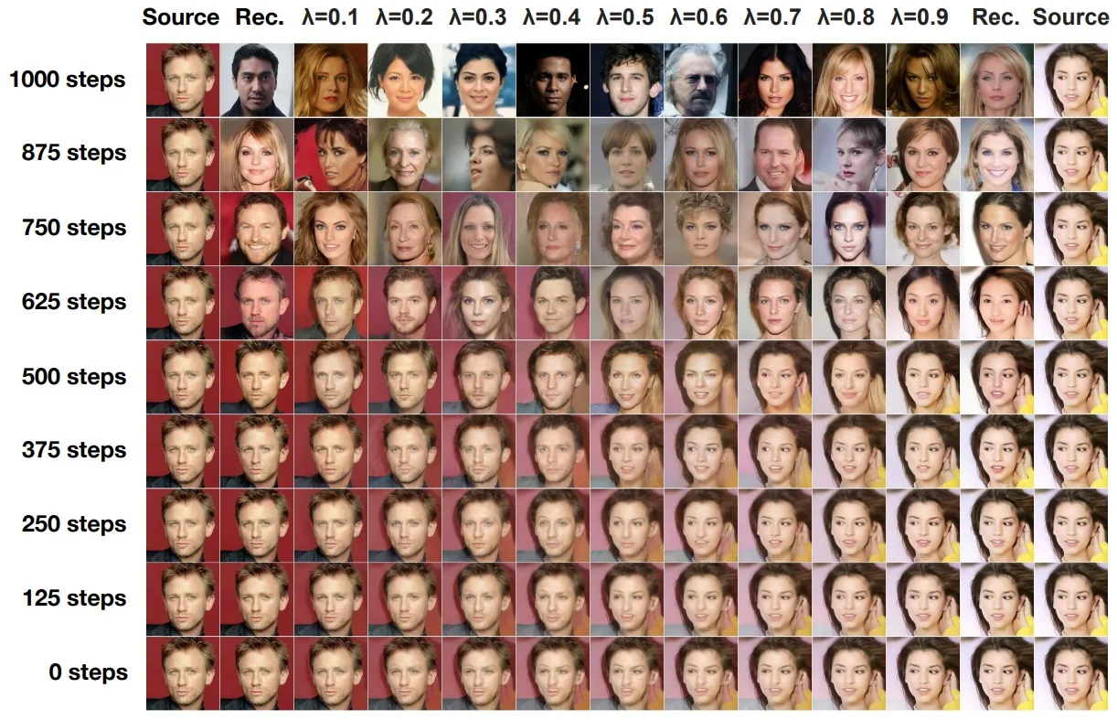
As shown in Figure 20.58, we observe:
- \( t = 0 \): Interpolation occurs directly in pixel space. The resulting images are unrealistic and far off-manifold, suffering from blurry blends and unnatural artifacts.
- \( t = 250 \): Fine-grained attributes (like expression, or hair texture) blend smoothly, but core identity remains distinct.
- \( t = 750 \): High-level semantic traits such as pose, facial structure, and lighting are interpolated. The model effectively recombines partial semantic cues from both images.
- \( t = 1000 \): The forward diffusion has fully erased both source images. The interpolated latent lies near the prior, and the reverse process generates novel samples that do not resemble either input — underscoring the destructive nature of high \( t \).
This experiment demonstrates that the forward diffusion process acts as a tunable semantic bottleneck. Small \( t \) values retain local details, enabling fine-grained morphing, while large \( t \) values eliminate low-level information, allowing the model to semantically complete or reinvent samples during denoising. Crucially, it reveals how diffusion models naturally support interpolation at different abstraction levels — from texture to structure — within a single framework.
Progressive Lossy Compression via Reverse Denoising Beyond interpolation, DDPMs enable an elegant form of semantic compression. By encoding images to a latent \( x_t \) via forward diffusion and decoding with \( p_\theta (x_0 \mid x_t) \), one can interpret \( x_t \) as a progressively degraded version of the original — retaining coarse structure at high \( t \), and finer details at lower \( t \).
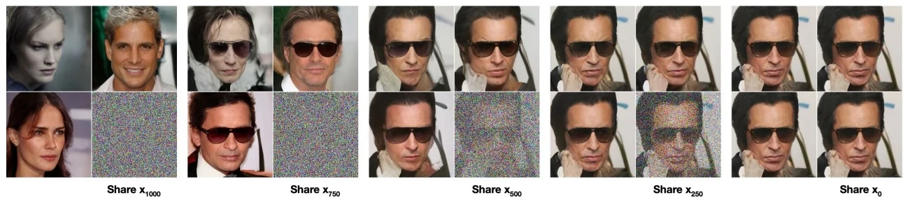
Figure 20.59 illustrates this behavior by fixing a latent \( x_t \) from a given source image and sampling multiple reconstructions at different noise levels. We observe:
- High \( t \) (e.g., 1000): Almost all detail is destroyed. Yet, all samples from \( p_\theta (x_0 \mid x_t) \) consistently reflect global properties such as face orientation and head shape — traits that persist deep into the diffusion process.
- Intermediate \( t \) (e.g., 750): Mid-level features like sunglasses, skin tone, or background begin to reemerge — attributes not present at \( t = 1000 \), but encoded in the intermediate latent.
- Low \( t \) (e.g., 500): Fine texture and local details (e.g., wrinkles, clothing patterns, eye sharpness) are reconstructed. The samples are perceptually similar and show near-lossless decoding.
This complements the earlier latent interpolation experiments: while Figure 20.57 and Figure 20.58 showed how DDPMs mix image content by interpolating between latents, Figure 20.59 focuses on what semantic content is recoverable from a given latent. Together, these experiments reveal that:
- The forward process acts as a progressive semantic bottleneck — discarding detail layer by layer, akin to a lossy compression encoder.
- The reverse process serves as a generative decoder, robustly reconstructing from incomplete information while respecting semantic priors.
- DDPMs naturally support multiple levels of abstraction — from global pose to pixel-level texture — controllable by the timestep \( t \).
Critically, these findings also validate the choice of noise prediction and fixed-variance reverse transitions (as shown in the ablation table): DDPMs not only achieve strong FID scores but exhibit robust, controllable behavior across a range of generation and compression tasks — without the need for external encoders or separate latent spaces.
Enrichment 20.9.3: Denoising Diffusion Implicit Models (DDIM)
Motivation While DDPMs can generate high-quality samples, their ancestral sampler is slow: it simulates a long reverse chain with many small denoising updates. The core cost is simply the number of iterations (often \(T\!=\!1000\)), not the network itself.
Denoising Diffusion Implicit Models (DDIM) [600] show that we can accelerate sampling without retraining by changing the inference-time trajectory. The key observation is that the usual DDPM training objective (e.g., the noise-prediction loss) depends on the marginals \(q(\mathbf {x}_t \mid \mathbf {x}_0)\), rather than on a single fixed choice of the full joint distribution \(q(\mathbf {x}_{1:T}\mid \mathbf {x}_0)\). DDIM exploits this “degree of freedom” by defining a non-Markovian diffusion process that preserves the same marginals \(q(\mathbf {x}_t \mid \mathbf {x}_0)\), but admits a reverse-time update that can skip timesteps and can be made deterministic.
Intuitively, DDIM replaces a long random walk of tiny steps with a shorter, structured trajectory that repeatedly (i) predicts what the clean image should be, and (ii) moves to an earlier noise level using that prediction.
From DDPM Sampling to DDIM Inversion To understand DDIM, start from the closed-form DDPM forward marginal: \[ q(\mathbf {x}_t \mid \mathbf {x}_0) = \mathcal {N}\!\left (\mathbf {x}_t;\, \sqrt {\bar {\alpha }_t}\mathbf {x}_0,\; (1-\bar {\alpha }_t)\mathbb {I}\right ), \] which can be reparameterized as \[ \mathbf {x}_t = \sqrt {\bar {\alpha }_t}\mathbf {x}_0 + \sqrt {1-\bar {\alpha }_t}\,\boldsymbol {\varepsilon }, \qquad \boldsymbol {\varepsilon }\sim \mathcal {N}(\mathbf {0},\mathbb {I}). \] This says that (for fixed \(t\)) \(\mathbf {x}_t\) can be viewed as a clean signal plus a single Gaussian “noise coordinate” \(\boldsymbol {\varepsilon }\).
Why DDIM can change the sampling process without retraining (theoretical backing). The crucial point is that DDPM training (under the common \(\boldsymbol {\varepsilon }\)-prediction objective) is organized around the marginals \(q(\mathbf {x}_t\mid \mathbf {x}_0)\): we sample \(t\), sample \(\boldsymbol {\varepsilon }\), form \(\mathbf {x}_t\) using the closed form above, and train \(\boldsymbol {\varepsilon }_\theta (\mathbf {x}_t,t)\) to recover the injected noise. This construction does not uniquely pin down a single “true” inference-time transition rule; many different (possibly non-Markovian) joint processes can share the same per-\(t\) marginals. DDIM exploits this degrees-of-freedom by defining an implicit inference rule that keeps the same marginals—hence stays compatible with the same trained denoiser—but allows skipping timesteps by coupling states through a shared latent noise coordinate \(\boldsymbol {\varepsilon }\).
During sampling we do not know \(\mathbf {x}_0\), so the denoiser predicts the noise: \[ \boldsymbol {\varepsilon }\approx \boldsymbol {\varepsilon }_\theta (\mathbf {x}_t,t), \] which yields a one-step estimate of the clean image: \[ \hat {\mathbf {x}}_0 = \frac {1}{\sqrt {\bar {\alpha }_t}} \left ( \mathbf {x}_t - \sqrt {1-\bar {\alpha }_t}\,\boldsymbol {\varepsilon }_\theta (\mathbf {x}_t,t) \right ). \]
Key consistency check (why the DDIM step is “right” when the denoiser is right). Suppose (idealized) that \(\boldsymbol {\varepsilon }_\theta (\mathbf {x}_t,t)=\boldsymbol {\varepsilon }\) equals the same latent noise coordinate that generated \(\mathbf {x}_t\), so that the estimator recovers \(\hat {\mathbf {x}}_0=\mathbf {x}_0\). Then, for any earlier \(s<t\), the forward marginal implies \[ \mathbf {x}_s = \sqrt {\bar {\alpha }_s}\mathbf {x}_0 + \sqrt {1-\bar {\alpha }_s}\,\boldsymbol {\varepsilon }. \] Replacing \((\mathbf {x}_0,\boldsymbol {\varepsilon })\) by \((\hat {\mathbf {x}}_0,\boldsymbol {\varepsilon }_\theta )\) therefore yields a reverse update that is exactly consistent with the same forward marginals in the perfect-model limit. This is the core theoretical intuition behind DDIM: the sampler is constructed to move along a trajectory parameterized by a shared latent noise coordinate, rather than resampling fresh noise at every intermediate step.
DDIM then defines a reverse update from \(t\) to an arbitrary earlier index \(s<t\) by combining (a projection of \(\hat {\mathbf {x}}_0\) to noise level \(s\)) with a compatible amount of predicted noise: \[ \mathbf {x}_s = \underbrace {\sqrt {\bar {\alpha }_s}\,\hat {\mathbf {x}}_0}_{\mbox{projected clean signal}} + \underbrace {\sqrt {1-\bar {\alpha }_s}\,\boldsymbol {\varepsilon }_\theta (\mathbf {x}_t,t)}_{\mbox{denoising direction}} \qquad (\mbox{deterministic DDIM}). \] At the next step, we feed \((\mathbf {x}_s,s)\) back into the network to obtain a new prediction \(\boldsymbol {\varepsilon }_\theta (\mathbf {x}_s,s)\), and repeat. This is where the speedup comes from: we choose a sparse schedule \(T=t_1>t_2>\cdots >0\) (e.g., 25–100 steps) and jump between those indices.
Optional stochasticity (\(\eta \)-continuum). DDIM also supports a stochastic extension by adding a tunable Gaussian term: \[ \mathbf {x}_s = \sqrt {\bar {\alpha }_s}\,\hat {\mathbf {x}}_0 + \sqrt {1-\bar {\alpha }_s-\sigma _{t\to s}^2}\,\boldsymbol {\varepsilon }_\theta (\mathbf {x}_t,t) + \sigma _{t\to s}\,\mathbf {z}, \qquad \mathbf {z}\sim \mathcal {N}(\mathbf {0},\mathbb {I}), \] where \(\sigma _{t\to s}\) is set using a scalar \(\eta \in [0,1]\): \(\eta =0\) gives the deterministic sampler, while larger \(\eta \) increases diversity and (for adjacent steps) recovers DDPM-like noise levels.
Why we do not always choose \(\eta = 0\) (fully deterministic). Deterministic DDIM (\(\eta =0\)) is attractive because it yields reproducible trajectories: for a fixed timestep schedule and initial noise \(\mathbf {x}_T\), the entire path \(\mathbf {x}_T \mapsto \cdots \mapsto \mathbf {x}_0\) is fixed [600]. However, always removing stochasticity is not universally desirable:
- Diversity as a controllable knob: In many applications we want multiple plausible samples for the same condition (class label / prompt) without changing the overall pipeline. Setting \(\eta >0\) reintroduces randomness in a principled way, producing a family of valid reverse trajectories and restoring DDPM-like variability as \(\eta \) increases [600].
- Hedging against model and discretization error: With aggressive timestep skipping, the reverse updates are larger and approximation errors can accumulate. Injecting a moderate amount of noise can act as a “robustness buffer”: instead of committing to a single deterministic correction at each step, the sampler explores a small neighborhood of plausible refinements consistent with the target noise level, which often improves qualitative stability when using very coarse schedules [600].
- Task-dependent preference: For editing and inversion-style workflows we often prefer \(\eta =0\) for consistency, while for unconditional or weakly conditioned generation we commonly prefer \(\eta >0\) to trade a bit of determinism for increased sample variety.
Why “inversion” is plausible (and why it remains approximate). When \(\eta =0\), the DDIM update rule defines a deterministic mapping between noise levels. This makes it natural to approximately invert a real image \(\mathbf {x}_0\) by running a corresponding deterministic procedure to obtain a compatible latent/noise representation and (optionally) a full diffusion trajectory \(\{\mathbf {x}_t\}_{t=0}^T\). Such DDIM inversions are widely used as an anchor for text-guided editing methods, which first invert an input image and then rerun generation under a modified condition while trying to preserve structure [226, 453]. Crucially, this inversion is not guaranteed to be exact: finite-step discretization and imperfect noise predictions mean that “invert then reconstruct” can drift, especially under coarse schedules.
In practice, this is handled by using sufficiently fine schedules for inversion and/or adding small post-hoc corrections (e.g., optimizing auxiliary conditioning) to better match the input image [453].
Forward pointer. Later, we will connect deterministic DDIM sampling to a continuous-time viewpoint that interprets \(\eta =0\) samplers as following a smooth, deterministic flow. For the present section, the key takeaway is operational: \(\eta \) provides a clean speed–diversity / determinism control knob, while keeping the same DDPM-trained denoiser.
We now derive the DDIM reverse (denoising) formula by walking through each conceptual and mathematical step.
1. From Forward Diffusion to Inversion The DDPM forward process defines a tractable Gaussian marginal at each timestep: \[ q(x_t \mid x_0) = \mathcal {N}\left ( \sqrt {\bar {\alpha }_t} \, x_0,\, (1 - \bar {\alpha }_t) \, \mathbb {I} \right ), \] which admits the following reparameterization: \[ x_t = \sqrt {\bar {\alpha }_t} \, x_0 + \sqrt {1 - \bar {\alpha }_t} \, \varepsilon , \qquad \varepsilon \sim \mathcal {N}(0, \mathbb {I}). \]
This expression is often called the “single-noise coordinate” view: for a fixed timestep \(t\), the noisy sample \(x_t\) can be decomposed into a (scaled) clean signal component and a (scaled) Gaussian noise component. Although the forward chain is implemented by injecting fresh Gaussian noise at each step, the closed-form marginal above implies that the distribution of \(x_t\) conditioned on \(x_0\) can always be represented using a single latent \(\varepsilon \) drawn from \(\mathcal {N}(0,\mathbb {I})\). DDIM will later exploit this perspective to define reverse transitions that keep a consistent noise coordinate across multiple steps, instead of re-sampling “fresh” randomness at every update.
If both \( x_t \) and \( \varepsilon \) are known, we can recover the original sample using: \[ x_0 = \frac {1}{\sqrt {\bar {\alpha }_t}} \left ( x_t - \sqrt {1 - \bar {\alpha }_t} \cdot \varepsilon \right ). \]
However, during sampling, we only observe the noisy sample \( x_t \). The clean image \( x_0 \) is unknown. To address this, the model is trained to approximate the injected noise: \[ \varepsilon \approx \varepsilon _\theta (x_t, t), \] allowing us to estimate the clean sample as: \[ \hat {x}_0 = \frac {1}{\sqrt {\bar {\alpha }_t}} \left ( x_t - \sqrt {1 - \bar {\alpha }_t} \cdot \varepsilon _\theta (x_t, t) \right ). \]
Why this particular prediction problem is “the right interface” for DDIM. A crucial point (which will become the main DDIM “loophole”) is that the training signal can be generated directly from the marginal \(q(x_t\mid x_0)\): sample \(x_0\) from the dataset, sample \(\varepsilon \sim \mathcal {N}(0,\mathbb {I})\), form \(x_t=\sqrt {\bar {\alpha }_t}x_0+\sqrt {1-\bar {\alpha }_t}\varepsilon \), and regress \(\varepsilon \) from \((x_t,t)\). This supervision recipe depends on the marginal noise level statistics \((\bar {\alpha }_t)\), not on a unique choice of joint factorization for the entire path \(x_0\!\rightarrow \!x_1\!\rightarrow \!\cdots \!\rightarrow \!x_T\). DDIM will keep the same marginals (hence the same training problem), but alter the inference-time transition rule.
This single-step estimate \( \hat {x}_0 \) may be inaccurate when \( t \) is large — that is, when \( x_t \) is heavily corrupted by noise and the denoising task is most difficult. Hence, DDIM continues with a multi-step procedure: starting from pure noise \( x_T \), it progressively refines samples \( x_t, \dots x_{s<t}, \dots , x_0 \) using noise prediction and noise reuse. We now derive the mechanism that enables this recursive denoising.
2. Reverse Step to Arbitrary \( s < t \) In DDPM, the reverse process is modeled as a Markov chain \[ x_T \rightarrow x_{T-1} \rightarrow x_{T-2} \rightarrow \dots \rightarrow x_0, \] where each step samples from a Gaussian distribution conditioned only on the previous timestep (“ancestral sampling”) [232]. This requires many small updates (typically \(T\!=\!1000\)) to gradually recover structure.
DDPM, made deterministic: you remove randomness, but you do not create a jump operator. If we “remove the new noise” in DDPM by setting the sampled Gaussian term to zero, we obtain a deterministic adjacent-step update. In the common \(\varepsilon \)-parameterization, the DDPM reverse mean is \[ x_{t-1} = \mu _\theta (x_t,t) = \frac {1}{\sqrt {\alpha _t}} \left ( x_t - \frac {1-\alpha _t}{\sqrt {1-\bar {\alpha }_t}}\, \varepsilon _\theta (x_t,t) \right ), \qquad (\mbox{deterministic DDPM: } z_t=0), \] with \(\alpha _t=1-\beta _t\). This is a local rule calibrated to the variance change from \(t\) to \(t-1\). So setting \(z_t=0\) changes stochasticity, but it does not change what the model actually specifies: a collection of adjacent-step Markov conditionals \(p_\theta (x_{t-1}\mid x_t)\), i.e., the only “legal move” it directly defines is \(t\!\to \!t-1\).
Why skipping is ill-defined within the DDPM Markov model (even if you set \(z=0\)). If you insist on staying in the same DDPM generative model and want to jump from \(x_t\) to \(x_s\) for \(s\ll t\), the correct conditional is the multi-step marginalization \[ p_\theta (x_s \mid x_t) = \int p_\theta (x_s \mid x_{s+1})\,p_\theta (x_{s+1}\mid x_{s+2})\cdots p_\theta (x_{t-1}\mid x_t)\,dx_{s+1:t-1}. \] This is generally intractable in closed form because the reverse means are state-dependent: to know the next mean you must first produce the intermediate state and then re-evaluate \(\varepsilon _\theta (x_{t-1},t-1)\), \(\varepsilon _\theta (x_{t-2},t-2)\), etc. Concretely, \(\varepsilon _\theta (x_{t-1},t-1)\) is not available unless we actually form \(x_{t-1}\), feed it to the network, then form \(x_{t-2}\), and so on.
This is the key point: skipping DDPM steps is not merely “remove noise and use a bigger step”. If you skip the intermediate evaluations, you are taking a large extrapolation using a direction field that would have been updated many times along the way. Empirically, this mismatch shows up as either (i) residual noise (wrong noise statistics at level \(s\)), or (ii) oversmoothing/blur (a conditional-mean compromise when the extrapolation drifts into high-uncertainty regions).
What DDIM changes: it replaces the transition operator itself. DDIM keeps the same trained denoiser \(\varepsilon _\theta \), but it redefines the inference-time generative process so that a direct map \(x_t \mapsto x_s\) is a first-class, explicitly defined operation [600]. The enabling observation is that the usual DDPM training objective depends on the forward marginals \(q(x_t\mid x_0)\), and many different joint paths (different intermediate conditionals) can share these same marginals [600]. DDIM exploits this freedom by using a non-Markovian (in \(x\) alone) inference model and a corresponding reverse rule that is directly evaluable for any \(s<t\).
DDIM jump, step-by-step: “decode \(\hat {x}_0\)” then “re-encode at level \(s\)”. Start from the closed-form marginal parameterization \[ x_t = \sqrt {\bar {\alpha }_t}\,x_0 + \sqrt {1-\bar {\alpha }_t}\,\varepsilon . \] At inference we do not know \((x_0,\varepsilon )\), but the network predicts a noise coordinate \(\hat {\varepsilon }_t := \varepsilon _\theta (x_t,t)\). Using the same algebra as the forward reparameterization, we form a clean-signal estimate \[ \hat {x}_0 = \frac {1}{\sqrt {\bar {\alpha }_t}} \left ( x_t - \sqrt {1-\bar {\alpha }_t}\,\hat {\varepsilon }_t \right ). \] DDIM then defines the (deterministic) jump to any \(s<t\) by re-encoding this \(\hat {x}_0\) to the target noise level \(s\) while reusing the same inferred noise coordinate: \[ x_s = \sqrt {\bar {\alpha }_s}\,\hat {x}_0 + \sqrt {1-\bar {\alpha }_s}\,\hat {\varepsilon }_t \qquad (\mbox{deterministic DDIM}). \] Equivalently, substituting \(\hat {x}_0\) gives an explicit map from \((x_t,t)\) to \(x_s\): \[ x_s = \sqrt {\frac {\bar {\alpha }_s}{\bar {\alpha }_t}}\,x_t + \left ( \sqrt {1-\bar {\alpha }_s} - \sqrt {\frac {\bar {\alpha }_s}{\bar {\alpha }_t}}\sqrt {1-\bar {\alpha }_t} \right )\hat {\varepsilon }_t. \] This is the concrete answer to “what changes?”: DDIM does not take the DDPM mean update and make it larger; it uses a different construction that explicitly targets the marginal noise level \(s\) via \(\bar {\alpha }_s\).
Crucially: even when \(s=t-1\), deterministic DDIM is generally not deterministic DDPM. Deterministic DDPM uses coefficients tied to \(\alpha _t\) and the one-step posterior form, whereas deterministic DDIM uses coefficients tied to \(\bar {\alpha }_{t-1}\) and the “re-encode” construction above. So DDIM is not “DDPM with \(z=0\)”; it is a different inference-time transition rule built from the same \(\varepsilon _\theta \).
How the trajectory changes (the intuition you were missing). Think of the forward identity \(x_t=\sqrt {\bar {\alpha }_t}x_0+\sqrt {1-\bar {\alpha }_t}\varepsilon \) as defining curves in image space: for a fixed pair \((x_0,\varepsilon )\), varying \(t\) traces one curve (only the coefficients change).
- DDPM (even deterministic) is “local stepping”. The model gives you a rule for moving one notch: \(t\!\to \!t-1\). The direction field must be recomputed at each new point (because \(\varepsilon _\theta (\cdot ,t)\) is evaluated on the current state). If you skip without those intermediate recomputations, you are applying a direction that is only valid locally and you drift off the appropriate “noise shell” for step \(s\), which is where blur/artifacts arise.
- DDIM is “latent-coordinate transport”. It first infers a global coordinate \((\hat {x}_0,\hat {\varepsilon }_t)\) from the current state, and then evaluates where that same coordinate would sit at the earlier noise level \(s\) by swapping coefficients from \((\bar {\alpha }_t)\) to \((\bar {\alpha }_s)\). That is why skipping is viable: the jump is an explicitly defined operator that lands at the correct marginal noise level by construction.
A 1D toy example makes this concrete. If \(x_t = a_t x_0 + b_t \varepsilon \) with \(a_t=\sqrt {\bar {\alpha }_t}\) and \(b_t=\sqrt {1-\bar {\alpha }_t}\), then knowing \((x_0,\varepsilon )\) makes any jump immediate: \(x_s = a_s x_0 + b_s \varepsilon \). DDIM approximates this by substituting \((x_0,\varepsilon )\mapsto (\hat {x}_0,\hat {\varepsilon }_t)\). DDPM does not provide an “evaluate at \(s\)” operator; it provides only a local adjacent-step rule that must be iterated.
Non-Markovian does not mean unprincipled: what information is carried across the jump. DDIM is non-Markovian in the visible variable \(x\) because \(x_s\) is allowed to depend on the inferred \(\hat {x}_0\) (equivalently \(\hat {\varepsilon }_t\)) [600]. A helpful mental model is that DDIM is Markovian in an augmented state that carries this global coordinate information, whereas DDPM enforces Markov structure in \(x_t\) alone. This extra global context is exactly what makes large jumps well-defined.
Why DDIM can stay sharp under coarse schedules, while naive DDPM skipping blurs. With DDPM, aggressive skipping effectively removes many intermediate “course-corrections” where the model would re-estimate \(\varepsilon _\theta (x_{t'},t')\) at progressively higher SNR. The resulting extrapolation behaves like a high-uncertainty compromise and tends toward oversmoothing. DDIM avoids this because each jump explicitly (i) places the sample at the correct marginal noise level \(s\) using \(\bar {\alpha }_s\), and (ii) follows a single inferred latent coordinate rather than implicitly averaging over many missing intermediate paths. Importantly, DDIM is still progressive: after jumping to \(x_s\), we feed \((x_s,s)\) back into the network to obtain \(\varepsilon _\theta (x_s,s)\) and refine the coordinate estimate, correcting accumulated error over the trajectory [600].
Summary (same network, different sampler). Both DDPM and DDIM reuse the same trained \(\varepsilon _\theta \). What changes is the sampler/transition operator: DDPM specifies only local adjacent-step Markov conditionals; removing noise only makes those local moves deterministic and does not define large jumps. DDIM redefines inference-time transitions via the “decode \(\hat {x}_0\), re-encode at level \(s\)” construction, making \(t\!\to \!s\) jumps a principled part of the inference model rather than an ad-hoc shortcut.
| DDPM: | \( x_T \to x_{T-1} \to x_{T-2} \to \dots \to x_1 \to x_0 \) | (adjacent-step Markov sampling) |
| DDIM: | \( x_T \to x_{t_1} \to x_{t_2} \to \dots \to x_1 \to x_0 \) | (explicit jumps; deterministic if \(\eta =0\)) |
Why not jump from \(x_T\) to \(\hat {x}_0\) in one step? Because at \(t\approx T\) the inversion is both ill-conditioned and underdetermined, and a one-shot estimate has no opportunity to self-correct.
- Ill-conditioning (tiny signal, huge amplification). When \(\bar {\alpha }_T\approx 0\), the clean component \(\sqrt {\bar {\alpha }_T}\,x_0\) barely affects \(x_T\). Even if \(\varepsilon _\theta (x_T,T)\) is reasonably accurate, turning it into a clean estimate requires dividing by \(\sqrt {\bar {\alpha }_T}\), which amplifies small denoiser errors. Write \(\varepsilon _\theta (x_T,T)=\varepsilon +\delta \). Then the implied clean estimate \( \hat {x}_0=\frac {x_T-\sqrt {1-\bar {\alpha }_T}\,\varepsilon _\theta (x_T,T)}{\sqrt {\bar {\alpha }_T}} \) obeys \[ \hat {x}_0-x_0 = -\frac {\sqrt {1-\bar {\alpha }_T}}{\sqrt {\bar {\alpha }_T}}\;\delta , \] so the error is scaled by \(\approx 1/\sqrt {\bar {\alpha }_T}\), which can be enormous at the terminal timestep. In plain terms: near pure noise, the algebraic “invert once” map is numerically unstable.
- Underdetermination (many \(x_0\) explain the same \(x_T\)). At \(t\approx T\), \(x_T\) contains almost no semantic evidence about which image was present before corruption. Equivalently, the posterior \(p(x_0\mid x_T)\) is extremely broad and highly multimodal: many very different clean images are compatible with essentially the same \(x_T\). A single-shot predictor must therefore choose a mode without sufficient information; under point-estimation behavior (e.g., MSE-style averaging in ambiguous regimes), this pressure can produce a washed-out “compromise” rather than a crisp committed sample.
-
No correction loop (one guess vs. a sequence of easier guesses). The key advantage of iterative sampling (DDPM or DDIM) is not just “more steps”: it is that each step increases the SNR and tightens the conditional.
After moving to a slightly less noisy state, the inverse problem becomes better conditioned and less ambiguous, and the next network call can correct earlier mistakes. A one-step jump from \(x_T\) commits to a single global estimate when uncertainty is maximal and provides no later opportunity to repair that commitment.
DDIM’s acceleration therefore comes from taking fewer, better-posed refinement steps—not from attempting the fundamentally unstable \(x_T\mapsto \hat {x}_0\) inversion in one shot. This motivates the next question: in what precise sense can we “reuse” a noise coordinate across a trajectory while still refining it step by step? We formalize that next.
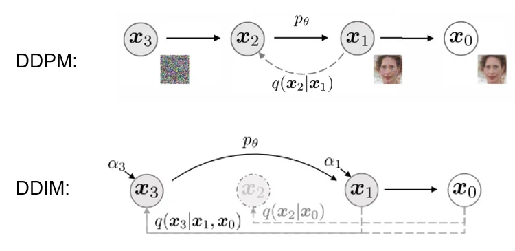
3. Why the “single–noise” picture is still correct The DDPM forward process injects fresh Gaussian noise at every step, defining a Markov chain \(q(x_t\mid x_{t-1})\). Superficially, this suggests that different independent noise variables govern each transition. DDIM’s viewpoint is that, although the implementation uses per-step noise, each marginal \(q(x_t\mid x_0)\) can be parameterized by a single Gaussian vector.
Key insight: forward marginals are closed-form. For any timestep \(t\), \[ q(x_t \mid x_0) = \mathcal {N}\!\left ( \sqrt {\bar {\alpha }_t}\,x_0,\; (1-\bar {\alpha }_t)\,I \right ), \] so we can reparameterize \[ x_t = \sqrt {\bar {\alpha }_t}\,x_0 + \sqrt {1-\bar {\alpha }_t}\,\varepsilon , \qquad \varepsilon \sim \mathcal {N}(0,I). \] Thus, for fixed \(x_0\) and \(t\), the random variable \(x_t\) can be generated from a single \(\varepsilon \); equivalently, \[ \varepsilon = \frac {x_t - \sqrt {\bar {\alpha }_t}\,x_0}{\sqrt {1-\bar {\alpha }_t}}. \] This does not contradict the Markov chain view; it simply states that the chain’s many independent noises collapse into one effective Gaussian coordinate at the level of the marginal.
DDPM training predicts this marginal noise coordinate. Under the standard noise-prediction objective, \[ \mathcal {L}_{\mathrm {simple}} = \mathbb {E}_{x_0,t,\varepsilon } \left \| \varepsilon - \varepsilon _\theta (x_t,t) \right \|^2, \] the network learns to recover the \(\varepsilon \) that (in the marginal view) generated \(x_t\). This is precisely the quantity DDIM reuses to define an alternative inference-time step.
DDIM’s deterministic reverse step (the \(\eta =0\) sampler). Given \(x_t\), we form \(\hat {x}_0\) via \[ \hat {x}_0 = \frac {1}{\sqrt {\bar {\alpha }_t}} \left ( x_t - \sqrt {1-\bar {\alpha }_t}\,\varepsilon _\theta (x_t,t) \right ), \] and then move to an earlier index \(s<t\) along the same marginal trajectory: \[ x_s = \sqrt {\bar {\alpha }_s}\,\hat {x}_0 + \sqrt {1-\bar {\alpha }_s}\,\varepsilon _\theta (x_t,t). \] Crucially, at the next step we recompute the noise coordinate by feeding \((x_s,s)\) back into the network to obtain \(\varepsilon _\theta (x_s,s)\). The sampler is therefore not “carrying” a fixed stored noise vector; rather, it repeatedly predicts a noise coordinate that is consistent with a single underlying trajectory.
Conclusion (what is and is not meant by “single-noise”):
- DDPM’s Markov chain uses independent noise increments, but each marginal \(q(x_t\mid x_0)\) admits a one-\(\varepsilon \) reparameterization.
- The objective \(\mathcal {L}_{\mathrm {simple}}\) trains \(\varepsilon _\theta (x_t,t)\) to recover that marginal noise coordinate from any \(x_t\).
- DDIM defines an alternative inference rule by combining \(\hat {x}_0\) with \(\varepsilon _\theta \), yielding a consistent (non-Markovian) trajectory compatible with DDPM training.
4. Optional Stochastic Extension (The \(\eta \)-Family) DDIM is not a single sampler, but a family of reverse-time update rules that all reuse the same trained denoiser \(\boldsymbol {\varepsilon }_\theta \). The key observation is that DDPM training constrains the forward marginals \(q(\mathbf {x}_t\mid \mathbf {x}_0)\) (equivalently, the linear-Gaussian relation between \(\mathbf {x}_0\) and \(\mathbf {x}_t\)), while leaving freedom in how we choose an inference-time joint path that is compatible with these marginals. DDIM exploits this flexibility to define reverse jumps \(t\!\to \! s\) (for any \(s<t\) in a sparse schedule) and to optionally inject additional “innovation” noise at test time.
Generalized reverse jump with controllable innovation noise. Let \(s<t\) denote the next index in a sampling schedule (possibly non-adjacent). DDIM decomposes the update into (i) a projected clean estimate, (ii) a deterministic noise component reused from the current state, and (iii) optional stochastic innovation: \begin {equation} \label {eq:chapter20_ddim_generalized_update} \mathbf {x}_s = \underbrace {\sqrt {\bar {\alpha }_s}\,\hat {\mathbf {x}}_0}_{\mbox{projected clean signal}} + \underbrace {\sqrt {1-\bar {\alpha }_s-\sigma _{t\to s}^2}\;\boldsymbol {\varepsilon }_\theta (\mathbf {x}_t,t)}_{\mbox{deterministic noise component}} + \underbrace {\sigma _{t\to s}\,\mathbf {z}}_{\mbox{stochastic innovation}}, \qquad \mathbf {z}\sim \mathcal {N}(\mathbf {0},\mathbf {I}). \end {equation} Here \(\hat {\mathbf {x}}_0\) is the standard “decode” estimate obtained by inverting the forward marginal at level \(t\): \begin {equation} \label {eq:chapter20_ddim_x0_pred} \hat {\mathbf {x}}_0(\mathbf {x}_t,t) = \frac {1}{\sqrt {\bar {\alpha }_t}} \left ( \mathbf {x}_t - \sqrt {1-\bar {\alpha }_t}\,\boldsymbol {\varepsilon }_\theta (\mathbf {x}_t,t) \right ). \end {equation}
The stochasticity knob \(\eta \in [0,1]\) and what it really controls. The parameter \(\eta \) scales the amount of fresh randomness injected by setting \begin {equation} \label {eq:chapter20_ddim_sigma_eta} \sigma _{t\to s}^2 = \eta ^2\left (\frac {1-\bar {\alpha }_s}{1-\bar {\alpha }_t}\right )\left (1-\frac {\bar {\alpha }_t}{\bar {\alpha }_s}\right ). \end {equation} This makes the interpolation completely explicit: increasing \(\eta \) continuously reallocates a portion of the “variance budget” at level \(s\) away from the reused (deterministic) component \(\sqrt {1-\bar {\alpha }_s-\sigma _{t\to s}^2}\,\boldsymbol {\varepsilon }_\theta (\mathbf {x}_t,t)\) and into independent innovation noise \(\sigma _{t\to s}\mathbf {z}\). In other words, \(\eta \) does not change the algebraic formula for \(\hat {\mathbf {x}}_0(\mathbf {x}_t,t)\) in (20.48); it changes the next state \(\mathbf {x}_s\) that the denoiser will see, and therefore changes the entire subsequent trajectory.
Why \(\eta \) matters even though \(\hat {\mathbf {x}}_0\) does not contain \(\eta \). For a fixed current state \(\mathbf {x}_t\), the map \(\mathbf {x}_t\mapsto \hat {\mathbf {x}}_0(\mathbf {x}_t,t)\) is the same for all \(\eta \). However, \(\eta \) changes \(\mathbf {x}_s\) through the innovation term, so the next denoiser call changes: \[ \mathbf {x}_t \;\xrightarrow [\eta ]{\mbox{update}}\; \mathbf {x}_s \;\xrightarrow {\;\boldsymbol {\varepsilon }_\theta (\cdot ,s)\;}\; \hat {\mathbf {x}}_0(\mathbf {x}_s,s) \;\xrightarrow {}\;\cdots \;\xrightarrow {}\; \mathbf {x}_0. \] Thus \(\eta \) changes which modes are explored, how much randomness accumulates, and how strongly the sampler “commits” to a single latent-coordinate trajectory.
Two anchor points (and what \(\eta =1\) does and does not mean).
- Deterministic DDIM (\(\eta =0\)). Then \(\sigma _{t\to s}=0\) and (20.47) becomes a purely deterministic transport of the current latent coordinate to level \(s\). This is the regime most directly associated with deterministic reverse-time flows (see below), and it is the regime that enables practical inversion/encoding behavior.
- Maximally stochastic within the DDIM family (\(\eta =1\)). This injects the largest innovation variance compatible with the target marginal at level \(s\). When the schedule uses adjacent steps (\(s=t-1\)), one recovers the usual DDPM posterior variance \[ \sigma _{t\to (t-1)}^2 = \frac {1-\bar {\alpha }_{t-1}}{1-\bar {\alpha }_t}\,\beta _t = \tilde {\beta }_t, \] so \(\eta =1\) coincides with standard DDPM-style ancestral sampling in that adjacent-step setting. For sparse schedules (\(s\ll t\)), \(\eta =1\) should be read as “maximally stochastic DDIM jumps” rather than “the original DDPM chain”: the transitions are no longer the DDPM Markov chain because the chain itself is not being traversed step-by-step.
Why choose \(\eta >0\) at all? What does it buy you? Even though sampling already starts from random \(\mathbf {x}_T\), \(\eta >0\) provides additional useful degrees of freedom:
- Diversity at fixed coarse structure. In conditional generation (and especially in image-to-image settings), one often wants multiple plausible “finishes” that preserve the same global layout. With \(\eta =0\), a fixed initial code and conditioning yields a single deterministic output; with \(\eta >0\), the injected \(\mathbf {z}\) creates multiple valid trajectories that share the same overall denoising direction but differ in fine details.
- A controllable fidelity–diversity trade-off. Small \(\eta \) keeps trajectories close to the deterministic transport (higher reproducibility and stronger structure preservation), while larger \(\eta \) injects more innovation and can reduce overly deterministic artifacts by exploring alternate paths. In practice, moderate \(\eta \) is sometimes used when one wants more “variety” without changing the model or the schedule.
- Hedging against model and discretization error. The deterministic path (\(\eta =0\)) places full trust in the denoiser’s prediction \(\boldsymbol {\varepsilon }_\theta (\mathbf {x}_t, t)\). However, this prediction is always imperfect. In a purely deterministic setting, a small directional error at step \(t\) permanently shifts the trajectory off the ideal data manifold, and subsequent steps can amplify this deviation (accumulation of error). Injecting a controlled amount of stochastic noise (\(\eta > 0\)) acts as a form of regularization or ”jitter”: it prevents the sampler from over-committing to a specific, potentially biased path. By continually ”shaking” the state into the local neighborhood of the prediction, the stochastic process helps average out systematic model errors, often resulting in more natural textures and fewer high-frequency artifacts than the rigid trajectory.
How does \(\eta \) interact with the number of sampling steps? The step count \(N\) is set by the schedule (how many indices you keep), not by \(\eta \). What \(\eta \) changes is how much new noise must be “paid off” by subsequent denoising. With very few steps (coarse schedules), injecting innovation noise can be harmful because there are not enough refinement steps left to reliably remove it; empirically, the deterministic regime \(\eta =0\) is often the most stable and highest-quality option when aggressively reducing \(N\). With more steps available, larger \(\eta \) becomes more feasible, because the chain has more opportunities to re-estimate \(\boldsymbol {\varepsilon }_\theta (\mathbf {x}_t,t)\) and correct the trajectory.
Preview: The Continuous-Time Limit (SDE vs. ODE). We have presented DDPM and DDIM as operations on discrete noise levels \(t\). However, there is a deeper mathematical interpretation that arises if we imagine the number of steps \(T\) approaching infinity.
- Stochastic (\(\eta > 0\)): The process behaves like a particle undergoing Brownian motion—a jagged ”random walk” that is slowly drifted toward the data manifold. We will later formalize this as a Stochastic Differential Equation (SDE).
- Deterministic (\(\eta = 0\)): The process behaves like a smooth, non-random fluid flow. This is known as the Probability Flow ODE.
Why this matters now: Even though we haven’t derived the equations yet, this distinction explains why DDIM allows for such aggressive acceleration. Because the deterministic path (\(\eta =0\)) defines a smooth, consistent curve rather than a chaotic random walk, it is much easier to approximate numerically. This allows us to replace simple step-by-step updates with advanced higher-order solvers (like Runge-Kutta) that can traverse the curve accurately in very few steps—a topic we will cover in depth in the upcoming section on Score-Based Generative Modeling.
DDIM Inversion: The Foundation of Image Editing. Determinism in DDIM (\(\eta =0\)) is not merely an aesthetic choice; it provides a functional advantage by defining a bijective mapping between the data distribution and the latent noise distribution. Because the underlying Probability Flow ODE is theoretically reversible, we can “invert” a real image \(\mathbf {x}_0\) by running the deterministic update rule backward (from \(t=0\) to \(t=T\)) to find its unique noise embedding \(\mathbf {x}_T\). This operation, known as DDIM Inversion, has become the backbone of modern text-guided editing pipelines [226].
The standard editing workflow exploits this structural consistency:
- 1.
- Invert: Map the input image \(\mathbf {x}_{\mbox{src}}\) to its latent noise \(\mathbf {x}_T\) using the source prompt.
- 2.
- Edit: Sample forward from \(\mathbf {x}_T\) using a modified prompt (e.g., changing “cat” to “dog”) or guidance scale.
Because the deterministic trajectory is governed by the same global noise coordinate, the edited image tends to preserve the spatial layout and composition of the original while adopting new semantic attributes.
Caveat: The accumulation of error. While the ODE is theoretically invertible, practical inversion is approximate due to discretization errors—the discrete forward step is not the exact mathematical inverse of the backward step. As a result, simply reconstructing \(\mathbf {x}_0\) from \(\mathbf {x}_T\) can lead to visual drift or artifacts. Advanced techniques like Null-Text Inversion [453] are often required to optimize the unconditional embeddings and correct these trajectory deviations, ensuring faithful reconstruction before editing.
A final geometric summary. Equation (20.47) keeps the target marginal “noise level” at \(s\) by construction. The first term inserts the current best clean estimate at level \(s\), the second term reuses the inferred latent coordinate to supply the remaining deterministic variance, and \(\eta \) decides how much of that variance is instead replaced by independent innovation noise. Thus \(\eta \) continuously interpolates between single-trajectory transport (\(\eta =0\)) and trajectory randomization (\(\eta >0\)), offering a tunable knob for speed–quality–diversity trade-offs without retraining.
5. Advantages of DDIM Sampling
- Deterministic inference: High-quality samples can be generated without randomness.
- Speedup: Fewer timesteps (e.g., 25, 50, or 100 instead of 1000) yield strong results.
- No retraining required: DDIM reuses DDPM-trained noise predictors.
- Trajectory consistency: Sampling follows the learned denoising direction.
- Tunable diversity: Optional variance allows DDPM-like diversity when needed.
The result is a more flexible sampling framework that enables both efficient and expressive image generation — a critical step toward scaling diffusion models in practice.
For further insights and ablations, we refer the reader to [600], which introduces DDIM and empirically benchmarks its improvements.
Enrichment 20.9.4: Guidance Techniques in Diffusion Models
Diffusion models offer a flexible generative framework, but in their basic formulation, sample generation proceeds unconditionally from Gaussian noise. In many real-world settings, we want to steer this generation process — for example, to condition on class labels, textual prompts, or other forms of side information. This general strategy is known as guidance.
Guidance techniques modify the reverse diffusion process to bias samples toward desired outcomes while retaining high sample quality. These approaches do not alter the forward noising process, and instead inject additional directional information into the sampling dynamics — often by adjusting the reverse transition rule.
We now explore several influential guidance strategies, beginning with the original classifier guidance method introduced by Dhariwal and Nichol [123].
Classifier Guidance
The first major form of guidance was introduced by Dhariwal and Nichol [123] under the name classifier guidance. It extends DDPMs to class-conditional generation by injecting semantic feedback from a pretrained classifier into the sampling dynamics of the reverse diffusion process.
During training, the denoising network \( \epsilon _\theta (x_t, t) \) is trained as usual to predict the noise added at each timestep, following the standard DDPM objective. Separately, a classifier \( p_\phi (y \mid x_t) \) is trained to predict labels from noisy images \( x_t \) at various timesteps \( t \in [0, T] \). This is achieved by minimizing a standard cross-entropy loss over samples from the noising process. The classifier is trained after or in parallel with the diffusion model, and remains fixed during guided generation.
At inference time, we generate a trajectory by progressively denoising \( x_T \sim \mathcal {N}(0, I) \) toward \( x_0 \), using the reverse Gaussian transitions modeled by the network. To bias generation toward a particular class \( y \), we modify the reverse step by incorporating the gradient of the log-probability \( \log p_\phi (y \mid x_t) \) with respect to the current sample \( x_t \). This yields a modified score function via Bayes’ rule: \[ \nabla _{x_t} \log p(x_t \mid y) = \nabla _{x_t} \log p(x_t) + \nabla _{x_t} \log p(y \mid x_t), \] where the first term is the score of the unconditional model, and the second term comes from the classifier. Since DDPMs already learn an approximation to \( \nabla _{x_t} \log p(x_t) \), we can guide sampling by simply adding the classifier gradient.
In score-based language, the noise prediction is adjusted as: \[ \hat {\epsilon }_{\mbox{guided}}(x_t, t) = \hat {\epsilon }_\theta (x_t, t) - s \cdot \Sigma _t \nabla _{x_t} \log p_\phi (y \mid x_t), \] where:
- \( \hat {\epsilon }_\theta (x_t, t) \) is the denoiser’s prediction of the added noise,
- \( \Sigma _t \) is the variance of the reverse diffusion step at time \( t \),
- \( s > 0 \) is a tunable guidance scale that controls how strongly the generation is biased toward class \( y \).
In practice, the classifier gradient \( \nabla _{x_t} \log p_\phi (y \mid x_t) \) is computed by backpropagating through the logits of a pretrained classifier \( p_\phi (y \mid x_t) \), using automatic differentiation.
During sampling, this is done as follows:
- 1.
- Given the current noisy sample \( x_t \) and the desired class \( y \), compute the classifier’s logit vector \( \ell = f_\phi (x_t) \in \mathbb {R}^C \), where \( C \) is the number of classes.
- 2.
- Extract the log-probability of the target class: \( \log p_\phi (y \mid x_t) = \log \mathrm {softmax}(\ell )_y \).
- 3.
- Backpropagate this scalar with respect to the input \( x_t \) (not with respect to the model weights) to obtain the gradient: \[ \nabla _{x_t} \log p_\phi (y \mid x_t). \]
- 4.
- Add this gradient to the score function, scaled by the guidance factor \( s \), to steer the reverse update toward class \( y \).
At first glance, it may seem problematic to alter the denoising trajectory learned by the model. After all, the diffusion model is trained to predict noise that reverses the corruption process from \( x_{t} \) to \( x_{t-1} \), and adding arbitrary gradients could in principle interfere with that process.
However, the addition of the classifier gradient is not arbitrary—it is theoretically grounded. We remind that the reverse diffusion process samples from the conditional distribution \( p(x_t \mid y) \), and its associated score function is: \[ \nabla _{x_t} \log p(x_t \mid y) = \nabla _{x_t} \log p(x_t) + \nabla _{x_t} \log p(y \mid x_t), \] by Bayes’ rule. The unconditional model learns to approximate \( \nabla _{x_t} \log p(x_t) \) through score estimation or noise prediction. Adding \( \nabla _{x_t} \log p(y \mid x_t) \), which comes from the classifier, completes the full class-conditional score.
Thus, the classifier gradient is not changing the direction arbitrarily—it is restoring a missing piece of the full score function required for class-conditional generation. The classifier acts like a plug-in module that injects semantic preference into the learned dynamics, gently pulling the sample trajectory toward regions where \( x_t \) is likely to belong to class \( y \), without disrupting the overall denoising process.
Empirically, this simple mechanism has been shown to substantially improve both perceptual quality and class accuracy, particularly at moderate-to-high guidance scales \( s \in [1, 15] \). It steers trajectories toward semantically meaningful modes in the conditional distribution, leading to clearer, sharper outputs—often at the cost of some diversity, which can be tuned via the scale \( s \).
This mechanism makes classifier guidance a plug-and-play enhancement: any differentiable classifier can be used, and the guidance strength \( s \) can be tuned at inference time to balance fidelity and diversity.
Although classifier guidance is simple to implement and produces significantly sharper and more class-consistent samples, it does come with two practical drawbacks: it requires training and storing a separate classifier over noisy images, and it introduces extra computation at sampling time due to gradient evaluations at every timestep. These limitations motivate the development of classifier-free guidance, which we discuss next.
Classifier-Free Guidance
While classifier guidance enables powerful class-conditional generation, it comes with practical drawbacks: it requires training and storing a separate classifier, and incurs additional gradient computations at each sampling step. To overcome these limitations, Ho and Salimans [233] proposed a remarkably simple alternative: classifier-free guidance.
The key idea is to let the denoising model itself learn both the unconditional and class-conditional scores. That is, instead of training a separate classifier to inject \( \nabla _{x_t} \log p(y \mid x_t) \), we extend the model input to optionally accept conditioning information and teach it to interpolate between both behaviors.
Training Procedure Let \( \epsilon _\theta (x_t, t, y) \) denote a noise prediction model that is explicitly conditioned on a class label \( y \). The classifier-free guidance technique trains this model to operate in both conditional and unconditional modes using a simple dropout strategy on the conditioning signal.
Concretely, during training we sample a data-label pair \( (x_0, y) \sim q(x, y) \), and select a timestep \( t \in \{1, \dots , T\} \). We generate a noisy input \( x_t = \sqrt {\bar {\alpha }_t} x_0 + \sqrt {1 - \bar {\alpha }_t} \epsilon \) where \( \epsilon \sim \mathcal {N}(0, I) \), and then choose a conditioning label as: \[ \tilde {y} = \begin {cases} y & \mbox{with probability } 1 - p_{\mbox{drop}}, \\ \varnothing & \mbox{with probability } p_{\mbox{drop}}, \end {cases} \] where \( \varnothing \) denotes an empty or null token indicating that no label is provided.
We then minimize the standard DDPM loss: \[ \mathbb {E}_{x_0, t, \epsilon , y} \left [ \left \| \epsilon _\theta (x_t, t, \tilde {y}) - \epsilon \right \|^2 \right ], \] thus training the model to perform both conditional and unconditional denoising, depending on whether \( \tilde {y} \) is real or masked. In practice, \( p_{\mbox{drop}} \in [0.1, 0.5] \) provides a good trade-off between learning both behaviors.
How the Conditioning \( y \) is Incorporated. The conditioning variable \( y \) must be integrated into the denoising model in a way that allows the network to modulate its predictions based on class information (or other forms of conditioning such as text). The implementation depends on the nature of \( y \):
- For discrete class labels (e.g., in class-conditional image generation), \( y \in \{1, \dots , C\} \) is typically passed through a learnable embedding layer: \[ e_y = \mbox{Embed}(y) \in \mathbb {R}^d. \] This embedding is then added to or concatenated with the timestep embedding \( e_t = \mbox{Embed}(t) \) and used to modulate the network. A common design is to inject \( e_y \) into residual blocks via adaptive normalization (e.g., conditional BatchNorm or FiLM [493]) or as additive biases.
- For richer conditioning (e.g., language prompts or segmentation masks), \( y \) may be a sequence or tensor. In such cases, the network architecture includes a cross-attention mechanism to allow the model to attend to the context: \[ \mbox{CrossAttn}(q, k, v) = \mbox{softmax}\left ( \frac {q k^\top }{\sqrt {d}} \right ) v, \] where the keys \( k \) and values \( v \) come from an encoder applied to the conditioning input \( y \), and the queries \( q \) are derived from the image representation.
These mechanisms allow the model to seamlessly switch between conditional and unconditional modes by simply masking or zeroing out the embedding of \( y \) during classifier-free training.
Sampling with Classifier-Free Guidance At inference time, we leverage the model’s ability to perform both conditional and unconditional denoising. Given a noisy input \( x_t \) at timestep \( t \), we evaluate the model under two scenarios:
\begin {align*} \epsilon _{\text {cond}} &= \epsilon _\theta (x_t, t, y), \\ \epsilon _{\text {uncond}} &= \epsilon _\theta (x_t, t, \varnothing ), \end {align*}
where \( y \) is the conditioning label (e.g., a class or prompt), and \( \varnothing \) denotes an unconditional (empty) input. These predictions are combined using the interpolation formula:
\[ \epsilon _{\mbox{guided}} = \epsilon _{\mbox{uncond}} + s \cdot \left ( \epsilon _{\mbox{cond}} - \epsilon _{\mbox{uncond}} \right ), \]
where \( s \geq 1 \) is the guidance scale controlling the strength of conditioning. This can also be written as:
\[ \epsilon _{\mbox{guided}} = (1 + s) \cdot \epsilon _{\mbox{cond}} - s \cdot \epsilon _{\mbox{uncond}}. \]
The following piece of code illustrates how class labels are embedded and applied inside a diffusion architecture (e.g., U-Net):
import torch
from tqdm import tqdm

# Assumes the following are pre-initialized:
# - model: diffusion model (e.g., U-Net)
# - text_encoder: a frozen CLIP/T5-style encoder
# - tokenizer: matching tokenizer
# - scheduler: DDPM or DDIM scheduler with .step()
# - guidance_scale: e.g., 7.5
# - H, W: image dimensions (e.g., 64x64)

# Step 1: Define prompt(s)
prompts = ["a photo of a dog"]  # List of text prompts
batch_size = len(prompts)
device = torch.device("cuda" if torch.cuda.is_available() else "cpu")

# Step 2: Tokenize conditional and unconditional prompts
cond_tokens = tokenizer(prompts, padding=True, return_tensors="pt")
uncond_tokens = tokenizer([""] * batch_size, padding=True, return_tensors="pt")

# Step 3: Encode prompts into embeddings
text_cond = text_encoder(
    input_ids=cond_tokens.input_ids.to(device),
    attention_mask=cond_tokens.attention_mask.to(device)
).last_hidden_state  # Shape: (B, T, D)

text_uncond = text_encoder(
    input_ids=uncond_tokens.input_ids.to(device),
    attention_mask=uncond_tokens.attention_mask.to(device)
).last_hidden_state  # Shape: (B, T, D)

# Step 4: Concatenate for a single forward pass
text_embeddings = torch.cat([text_uncond, text_cond], dim=0)  # Shape: (2B, T, D)

# Step 5: Initialize Gaussian noise
x = torch.randn((2 * batch_size, model.in_channels, H, W), device=device)

# Step 6: Reverse sampling loop
for t in tqdm(scheduler.timesteps):
    t_batch = torch.full((2 * batch_size,), t, device=device, dtype=torch.long)

    with torch.no_grad():
        noise_pred = model(x, t_batch, encoder_hidden_states=text_embeddings).sample
        noise_uncond, noise_cond = noise_pred.chunk(2)  # Split into (B, ...) chunks

        # Apply classifier-free guidance
        guided_noise = noise_uncond + guidance_scale * (noise_cond - noise_uncond)

    # Step the scheduler using only guided samples
    x = scheduler.step(guided_noise, t, x[:batch_size]).prev_sample  # Shape: (B, C, H, W)
This simple pattern is powerful and generalizes across different modalities. In more complex systems such as Stable Diffusion [548], the conditional input \( y \) is often a text prompt embedded using a frozen transformer like CLIP [512], and passed through multiple layers of cross-attention throughout the U-Net decoder.
Why Classifier-Free Guidance Works: A Score-Based and Intuitive View Classifier-Free Guidance (CFG) builds on a simple yet powerful idea: train a single diffusion model to support both unconditional and conditional denoising behaviors. By exposing the model to both kinds of inputs during training, it becomes possible to steer generation toward a semantic target \( y \) without relying on a separate classifier.
To understand this, consider the decomposition of the conditional log-probability using Bayes’ rule: \begin {equation} \log p(x_t \mid y) = \log p(x_t) + \log p(y \mid x_t). \end {equation} Taking the gradient with respect to \( x_t \) yields: \begin {equation} \nabla _{x_t} \log p(x_t \mid y) = \nabla _{x_t} \log p(x_t) + \nabla _{x_t} \log p(y \mid x_t). \end {equation}
This tells us that the conditional score consists of two components:
- an unconditional score \( \nabla _{x_t} \log p(x_t) \), which represents the direction that increases likelihood under the overall data distribution;
- a label-specific influence \( \nabla _{x_t} \log p(y \mid x_t) \), which corrects the direction based on the conditioning variable \( y \).
In classifier guidance, the second term is approximated by a trained classifier. In classifier-free guidance, however, both terms are learned by the same model through a clever training trick: randomly dropping the conditioning label \( y \) (e.g., with 10% probability) and training the model to denoise in both settings.
Specifically:
- When \( y = \texttt{"dog"} \), the model sees noisy dog images \( x_t \) and learns to denoise them toward clean images \( x_0 \), guided by the label.
- When \( y \) is dropped, the model learns unconditional denoising: predicting \( x_0 \) without any external label.
As a result, the model implicitly learns: \begin {align} s_\theta (x_t, y, t) &\approx \nabla _{x_t} \log p(x_t \mid y), \quad \text {(conditional score)} \\ s_\theta (x_t, \varnothing , t) &\approx \nabla _{x_t} \log p(x_t), \quad \text {(unconditional score)} \end {align}
Subtracting these gives an approximation of the label’s effect: \begin {equation} s_\theta (x_t, y, t) - s_\theta (x_t, \varnothing , t) \approx \nabla _{x_t} \log p(y \mid x_t). \end {equation}
Intuition: This subtraction isolates the direction in feature space that pushes a sample toward better alignment with label \( y \). It’s as if we are extracting the “semantic vector field” attributable to the label alone. By multiplying this vector by a scale factor \( s \), we can amplify movement in the direction of the conditioning label.
Substituting into Bayes’ decomposition gives: \begin {equation} \nabla _{x_t} \log p(x_t \mid y) \approx s_\theta (x_t, \varnothing , t) + s \cdot \left ( s_\theta (x_t, y, t) - s_\theta (x_t, \varnothing , t) \right ), \end {equation} where \( s \in \mathbb {R}_{\geq 0} \) is a user-defined guidance scale.
In practice, most diffusion models are trained to predict noise \( \epsilon \) rather than the score directly. This reasoning therefore translates into the widely-used noise prediction rule: \begin {equation} \epsilon _{\mbox{guided}} = \epsilon _{\mbox{uncond}} + s \cdot \left ( \epsilon _{\mbox{cond}} - \epsilon _{\mbox{uncond}} \right ), \end {equation} where \( \epsilon _{\mbox{cond}} = \epsilon _\theta (x_t, t, y) \) and \( \epsilon _{\mbox{uncond}} = \epsilon _\theta (x_t, t, \varnothing ) \).
Conclusion. By training the model on noisy samples paired with and without the label, it learns how the presence of \( y \) modifies the denoising direction. At inference time, we explicitly compute and amplify this direction by subtracting the unconditional prediction and scaling the result. This lets us generate samples that are more aligned with the target concept, while preserving the stability of the underlying diffusion process.
Interpretation The difference \( \epsilon _{\mbox{cond}} - \epsilon _{\mbox{uncond}} \) approximates the semantic shift introduced by conditioning on \( y \). Scaling this difference by \( s \) amplifies the class- or prompt-specific features in the output, steering the model’s trajectory toward the desired mode. Larger values of \( s \) increase class adherence but may reduce diversity, reflecting a precision-recall trade-off in generation.
Typical Settings Empirically, guidance scales \( s \in [7.5, 10] \) often strike a good balance between fidelity and variation. Values \( s > 10 \) can produce oversaturated or collapsed samples, while \( s = 0 \) corresponds to pure unconditional generation.
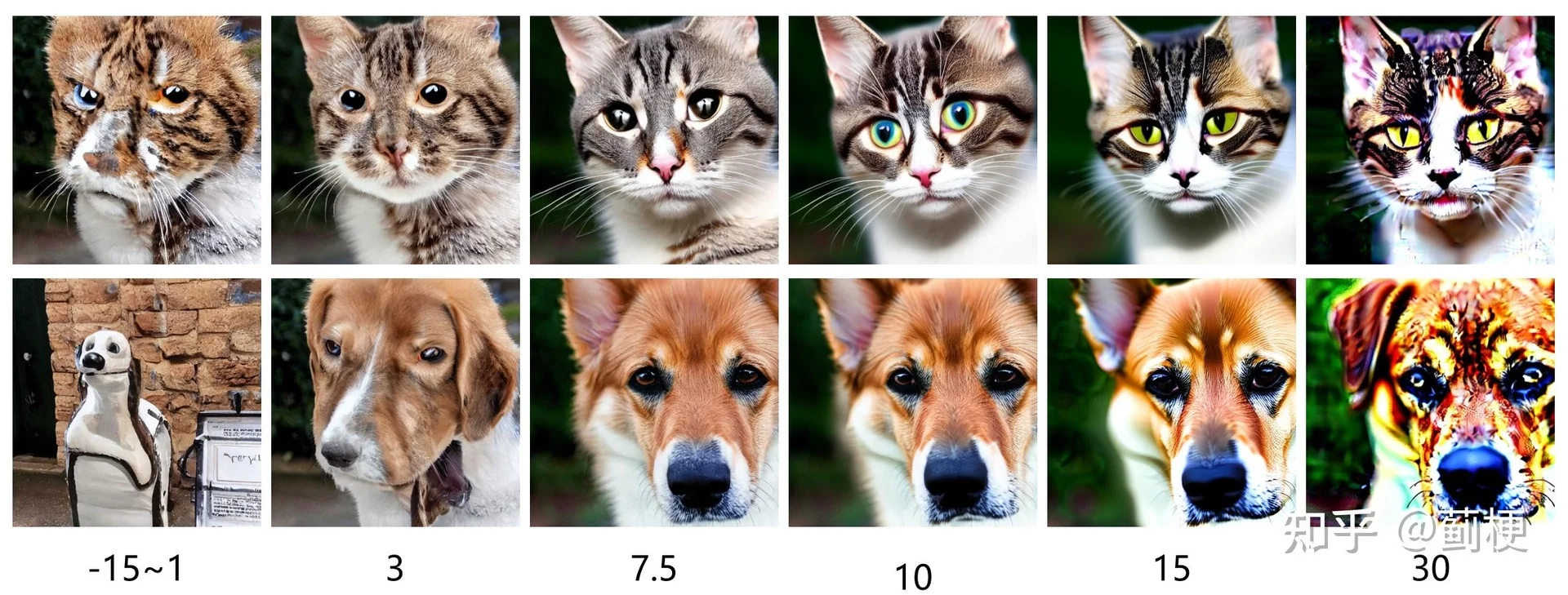
Advantages Classifier-free guidance has become a cornerstone of modern diffusion-based systems because:
- It requires no auxiliary classifier: Conditioning is integrated directly into the denoiser, making the architecture self-contained.
- It avoids expensive gradient computations: No backward pass is needed during sampling.
- It enables dynamic guidance strength: Users can modulate \( s \) at test time without retraining the model.
- It generalizes beyond classes: The same technique applies to text prompts, segmentation maps, audio inputs, or any other conditioning.
Adoption in Large-Scale Models Classifier-free guidance is now standard in most large-scale diffusion pipelines, including:
- Imagen [557], which uses language conditioning on top of a super-resolution cascade,
- Stable Diffusion [548], where text embeddings from CLIP guide an autoencoding UNet,
- DALLE-2 [524], which uses CFG to synthesize and refine images from textual prompts.
This generality makes it one of the most practical and powerful tools for guided generative modeling with diffusion models.
Enrichment 20.9.5: Cascaded Diffusion Models
Motivation and Overview Diffusion models can generate extremely high-fidelity images, but direct high-resolution generation (e.g., \(256\times 256\) and beyond) is expensive and difficult: the model must simultaneously represent global composition (long-range structure) and fine-grained texture, and the denoising network must process large spatial tensors at every reverse step.
Cascaded Diffusion Models (CDMs) [234] address this by factorizing generation across resolutions. A CDM is a pipeline of separately trained diffusion models that generate images of increasing resolution: a low-resolution base diffusion model produces a coarse sample, and one or more super-resolution diffusion models (SR models) progressively upsample and add detail.
A common ImageNet cascade is:
- 1.
- Base model (lowest resolution, e.g., \(32\times 32\)): sample \(x_0^{(32)} \sim p_\theta (x_0 \mid y)\) from Gaussian noise, conditioned on the class label \(y\).
- 2.
- SR model 1 (e.g., \(32\to 64\)): sample \(x_0^{(64)} \sim p_\theta (x_0 \mid y, z^{(32\to 64)})\), where \(z\) is an upsampled low-resolution conditioning image derived from the previous stage.
- 3.
- SR model 2 (e.g., \(64\to 256\)): sample \(x_0^{(256)} \sim p_\theta (x_0 \mid y, z^{(64\to 256)})\), again conditioning on an upsampled output from the previous stage.
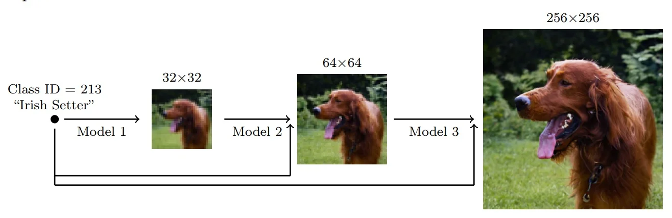
The central challenge: compounding error (exposure bias). A cascade is only as good as the conditioning it passes forward: at training time, SR models condition on clean low-resolution images derived from real data, but at test time they condition on generated low-resolution samples. This train–test mismatch can cause errors to compound across stages.
The central fix: conditioning augmentation. CDMs rely crucially on conditioning augmentation—strong augmentation applied to the low-resolution conditioning input \(z\) during training—to make SR models robust to imperfect upstream samples [234]. Intuitively, SR models are trained to succeed even when the coarse guide is “noisy” or “imprecise”, so test-time generated guides do not derail the cascade.
This decomposition yields:
- Scalability: each model only processes a manageable spatial resolution.
- Specialization: low-res models focus on global semantics; SR models focus on texture/detail consistent with a coarse layout.
- Modularity: stages can be improved, ablated, or replaced independently.
In the following parts, we describe (i) the U-Net conditioning design (including how \(t\) and \(y\) are injected), (ii) conditioning augmentation and why it is necessary, and (iii) the training and inference pipeline for high-resolution cascaded sampling.
Architecture: U-Net Design for Cascaded Diffusion Models Each stage in a CDM—the base model and every super-resolution (SR) model—is implemented as a time-conditioned U-Net denoiser. The U-Net provides (i) a multi-scale feature hierarchy for global context and (ii) skip connections for spatial fidelity.
How conditioning enters the network. At a given SR stage, the model is trained to denoise a noisy target-resolution image \(x_t\) while being guided by: (i) the class label \(y\) and (ii) a low-resolution conditioning image \(z\) derived from the previous stage. Concretely, \(z\) is deterministically upsampled to the target resolution and then concatenated channel-wise with \(x_t\) at the U-Net input [234]. Scalar condition signals (timestep \(t\), class label \(y\), and sometimes augmentation-level metadata) are embedded and injected throughout the U-Net’s residual blocks so that every scale “knows” the current noise level and semantic target.
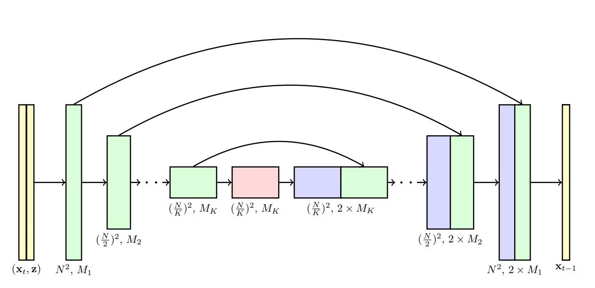
Inputs and Their Roles in CDM Super-Resolution Models
Each super-resolution stage in a Cascaded Diffusion Model (CDM) functions as a conditional denoiser. Unlike naive super-resolution, which might learn a direct mapping from low-res to high-res, CDM stages begin from noise and learn to sample a distribution over plausible refinements, guided by a coarser input.
- Noisy high-resolution image \( x_t \): This is a sample from the standard forward diffusion process: \[ x_t = \sqrt {\bar {\alpha }_t} \, x_0 + \sqrt {1 - \bar {\alpha }_t} \, \epsilon , \qquad \epsilon \sim \mathcal {N}(0, I). \] Here, \( x_0 \) is a clean high-resolution image from the dataset, and \( t \in [0, 1] \) is a timestep. The model is trained to denoise \( x_t \) using information from the timestep \( t \), the class label \( y \), and a coarse guidance image \( z \). This preserves the probabilistic nature of generation: the network learns to sample detailed content rather than deterministically sharpen \( z \).
-
Low-resolution guide \(z\) (structure anchor, and why it is augmented): The guide \(z\) is a deterministic, low-frequency “layout” image that anchors the high-resolution sample to the coarse structure already chosen by the previous stage. During training, it is constructed from a real target image \(x_0\) by (i) downsampling \(x_0\) to the previous stage resolution and then (ii) upsampling back to the current resolution (e.g., bilinear), producing a blurred, low-detail version of \(x_0\).
Conditioning augmentation (crucial for cascades). At test time, the SR model conditions on generated low-resolution samples, which are imperfect. To prevent errors from compounding across stages, CDMs apply strong augmentation to the conditioning input during training [234]. Concretely, one trains the SR denoiser to succeed even when the guide is perturbed (e.g., by Gaussian noise at low-resolution upsampling, or blur at high-resolution upsampling), so that imperfect generated guides at inference are “in-distribution” for the SR model. This is the main mechanism that alleviates exposure bias / train–test mismatch in cascaded sampling [234].
- Timestep conditioning \(t\) (where it enters the U-Net): In the standard discrete-time formulation, we sample a timestep \(t \in \{1,\dots ,T\}\), where larger \(t\) means lower SNR (more corruption) and smaller \(t\) means higher SNR (finer denoising). The scalar \(t\) is mapped to a vector embedding (typically sinusoidal features followed by an MLP), and this embedding is injected throughout the U-Net’s residual blocks. Operationally, this makes the denoiser a family of functions indexed by noise level: early blocks learn “coarse semantic cleanup” at high noise, while late blocks learn “texture-preserving refinement” at low noise. Without \(t\), the same input \(x_t\) would be ambiguous because the appropriate denoising strength depends on how much noise was added.
- Class label \( y \): In class-conditional setups, the label is embedded (e.g., via a learned embedding table or projection) and added to intermediate layers in the U-Net—often by adding it to the same intermediate representation as \( t \). This helps guide the generation toward the correct semantic category.
Mechanism: Adaptive Group Normalization (AdaGN). How do a single scalar timestep \( t \) and class label \( y \) control the behavior of a massive U-Net? They do not merely append data; they modulate the network’s internal feature statistics.
- 1.
- Embedding: First, \( t \) is mapped to a high-dimensional vector via sinusoidal positional encodings (similar to Transformers), and \( y \) is mapped via a learned lookup table. These are combined (e.g., summed) into a global context vector \( \mathbf {c} \).
- 2.
- Projection: Inside each residual block, a lightweight MLP projects \( \mathbf {c} \) into two scale-and-shift vectors, \( \boldsymbol {\gamma }(\mathbf {c}) \) and \( \boldsymbol {\beta }(\mathbf {c}) \), matching the channel dimension of the feature map \( \mathbf {h} \).
- 3.
- Modulation: These vectors modulate the normalized features via an affine transformation: \[ \mathrm {AdaGN}(\mathbf {h}, \mathbf {c}) = \boldsymbol {\gamma }(\mathbf {c}) \odot \mathrm {GroupNorm}(\mathbf {h}) + \boldsymbol {\beta }(\mathbf {c}). \]
Intuition. Think of \( \boldsymbol {\gamma } \) and \( \boldsymbol {\beta } \) as dynamic ”volume knobs” for each feature channel. At high noise levels (large \( t \)), the network might suppress high-frequency texture channels and amplify low-frequency shape detectors. As \( t \to 0 \), the embedding changes, rotating the ”knobs” to activate texture-refining filters instead. This mechanism allows a single set of shared weights to function as a sequence of distinct operators—coarse generation first, fine refinement later—driven entirely by the global scalar signal.
Why Are Both \( x_t \) and \( z \) Needed?
Super-resolution diffusion models are trained to sample diverse, high-resolution outputs consistent with a low-res guide. These two inputs serve complementary roles:
- \( x_t \) introduces stochasticity—the model learns a distribution over high-res reconstructions, not a fixed sharpening process. Sampling from noise also enables diversity in outputs.
- \( z \) provides structural anchoring—it ensures that sampled outputs respect the layout, pose, and semantic structure already determined at the previous stage.
While it may seem redundant to denoise \( x_0 \) (which is already high-res), recall that we are not simply reconstructing \( x_0 \) deterministically—we are learning to sample high-resolution images consistent with \( z \). This formulation ensures that each CDM stage acts like a generative model in its own right, capable of producing diverse samples even when guided.
Training Procedure (SR stage, with conditioning augmentation):
Each super-resolution model is trained independently as a conditional diffusion denoiser:
- 1.
- Sample a clean target image \(x_0 \in \mathbb {R}^{H \times W \times C}\) at the stage resolution (e.g., \(64\times 64\) or \(256\times 256\)).
- 2.
- Construct the low-resolution guide \(z\) by downsampling \(x_0\) to the previous stage resolution and upsampling back to \((H,W)\).
- 3.
- Apply conditioning augmentation to obtain an augmented guide \(\tilde {z}\) (e.g., add Gaussian noise for low-resolution upsampling, or blur for high-resolution upsampling), so the SR model learns robustness to imperfect upstream samples [234].
- 4.
- Sample a timestep \(t \sim \mathrm {Uniform}(\{1,\dots ,T\})\) and noise \(\boldsymbol {\varepsilon }\sim \mathcal {N}(0,I)\), then form \[ x_t = \sqrt {\bar {\alpha }_t}\,x_0 + \sqrt {1-\bar {\alpha }_t}\,\boldsymbol {\varepsilon }. \]
- 5.
- Train the denoiser to predict the injected noise: \[ \mathbb {E}_{x_0,t,\boldsymbol {\varepsilon },\tilde {z},y} \big [ \|\boldsymbol {\varepsilon }_\theta (x_t,t,\tilde {z},y)-\boldsymbol {\varepsilon }\|_2^2 \big ]. \]
Inference Pipeline (sequential sampling across resolutions):
Sampling from a CDM proceeds sequentially across stages:
- 1.
- Base stage (lowest resolution, e.g., \(32\times 32\)): initialize \(x_T^{(\mathrm {low})}\sim \mathcal {N}(0,I)\) and run a reverse-time sampler (DDPM-style or DDIM-style schedule) to obtain \(\tilde {x}_0^{(\mathrm {low})}\sim p_\theta (x_0\mid y)\).
- 2.
- Super-resolution stages (increasing resolution): for each SR model in
order:
- (a)
- Upsample the previous output to form the conditioning guide \(z\).
- (b)
- Optionally apply the same type of perturbation used during training (conceptually: the SR model has been trained to tolerate a “noisy/blurred/imperfect” guide), so errors do not compound across the cascade [234].
- (c)
- Initialize fresh noise \(x_T^{(\mathrm {high})}\sim \mathcal {N}(0,I)\) at the target resolution and run the SR denoising loop conditioned on \((z,y)\) to obtain \(\tilde {x}_0^{(\mathrm {high})}\).
Each stage is itself a full diffusion sampler at its own resolution; the cascade simply chooses to allocate “global semantics” to low resolutions and “texture/detail” to later SR stages, while conditioning augmentation makes the handoff between stages robust [234].
Each stage performs a complete generation pass at its resolution: the base model synthesizes the semantic structure, and subsequent models enhance visual fidelity and fine details. Because the input noise \( x_T \) is sampled independently at each stage, and the conditioning image \( z \) is fixed throughout the reverse process, the pipeline is modular and supports parallel improvements at each resolution level.
Empirical Performance of CDMs A key empirical takeaway of [234] is that high-fidelity cascaded sampling is achievable without auxiliary classifiers, but only when the SR stages are trained with strong conditioning augmentation to avoid compounding error across the pipeline.
On class-conditional ImageNet generation, the paper reports that CDMs achieve FID scores of \(1.48\) at \(64\times 64\), \(3.52\) at \(128\times 128\), and \(4.88\) at \(256\times 256\) [234]. Beyond perceptual quality, CDM samples are also highly class-consistent: at \(256\times 256\), the reported classification accuracy of generated samples reaches \(63.02\%\) Top-1 and \(84.06\%\) Top-5 [234]. These numbers reflect the intended division of labor in the cascade: early stages commit to the correct global semantics, while later SR stages add detail without drifting away from the established layout.
Why the cascade helps (interpretation). The cascade reduces a hard global problem (generate a coherent \(256\times 256\) image from noise) into multiple easier problems: (i) choose the coarse semantic configuration at low resolution, then (ii) sample plausible high-frequency refinements conditioned on that configuration. Conditioning augmentation is what makes this decomposition stable in practice: it trains SR models to remain reliable even when the low-resolution conditioning image is an imperfect generated sample rather than a clean downsample of real data [234].
Enrichment 20.9.6: Progressive Distillation for Fast Sampling
Diffusion models produce high-quality samples, but their main practical drawback is slow sampling: generating one image can require hundreds to thousands of sequential network evaluations. A naïve attempt to “skip steps” by learning a large-jump denoiser tends to produce blurry outputs, because many distinct clean images can map to similar noisy latents, so an unconstrained large-step predictor averages over plausible reverse trajectories.
Progressive distillation [559] avoids this failure mode by distilling a specific high-quality trajectory. The starting point is a strong deterministic sampler (DDIM), which can be viewed as an integration rule for the probability flow ODE. Rather than asking a student to invent a new coarse trajectory, we train it to match the teacher’s dynamics: each student step is trained to reproduce the effect of two teacher DDIM steps over the same time interval. This yields a sharp, teacher-determined target at each noisy state, preventing the conditional-averaging that causes blur.
By repeating this halving procedure (e.g., \(8192\!\to \!4096\!\to \!2048\!\to \!\dots \!\to \!4\) steps), we progressively amortize numerical integration into fewer learned updates, achieving orders-of-magnitude speedups while largely preserving perceptual quality.
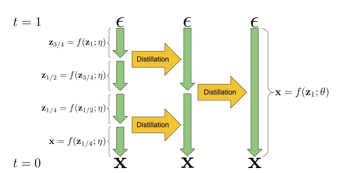
Pseudocode: Progressive Distillation Loop Progressive distillation [559] reduces sampling cost by repeatedly halving the number of inference steps. Fix a student step budget \(N\), so each student update jumps one coarse interval of size \(1/N\) in normalized time. For supervision, the teacher constructs a finer deterministic DDIM trajectory over the same coarse interval by taking two substeps of size \(0.5/N\). The student is then trained so that one of its coarse steps reproduces the endpoint of those two teacher substeps. After convergence, the student is promoted to become the next teacher and we halve \(N\).
Discrete-time convention and why we use \(t=i/N\). Unlike the original diffusion training, progressive distillation is run in discrete time: we select a step budget \(N\), define the time grid \(\{i/N\}_{i=1}^N\subset (0,1]\), and sample an index \(i\sim \mathrm {Unif}\{1,2,\dots ,N\}\) (discrete uniform) so that all noise levels are seen during training. The endpoint \(t=1\) is chosen so that \(\alpha _1=0\) and therefore \(z_1\sim \mathcal {N}(0,I)\), exactly matching the test-time input distribution of the sampler [559].
Inputs: trained teacher denoiser \(\hat {x}_\eta (z_t,t)\), dataset \(\mathcal {D}\), loss weight function \(w(\lambda _t)\), initial student step budget \(N\), learning rate \(\gamma \), schedule \(\alpha _t,\sigma _t\) with \(\alpha _1=0\) (so \(z_1\sim \mathcal {N}(0,I)\)).
- 1.
- While \(N\) is larger than the desired final budget (e.g. stop when
\(N=4\)):
- (a)
- Initialize student from teacher: \(\theta \leftarrow \eta \).
- (b)
- While not converged:
- i.
- Sample a clean training image \(x \sim \mathcal {D}\).
- ii.
- Sample a discrete time index \(i \sim \mathrm {Unif}\{1,2,\dots ,N\}\) and set \(t=i/N\). Here \(\mathrm {Unif}\{1,\dots ,N\}\) denotes the uniform distribution over the \(N\) sampling intervals, so that each student update (from one coarse time grid point to the next) is trained with comparable frequency, as in Algorithm 2 of [559].
- iii.
- Sample noise \(\epsilon \sim \mathcal {N}(0,I)\) and form the noisy input \[ z_t = \alpha _t x + \sigma _t \epsilon . \] Interpretation: \(\alpha _t\) controls the remaining signal energy and \(\sigma _t\) controls the injected noise energy. Under the cosine schedule (below), \(\alpha _t^2+\sigma _t^2=1\), so \(\alpha _t\) decreases smoothly from \(1\) to \(0\) while \(\sigma _t\) increases from \(0\) to \(1\).
- iv.
- Two teacher DDIM substeps over the same coarse
interval. The student is being trained to make one coarse
deterministic DDIM jump from \(t\) to \[ t'' \;=\; t-\frac {1}{N}. \] To produce a sharper
supervision signal than “denoise toward \(x\)”, the teacher
traverses the same interval using two equal substeps of size
\(1/(2N)\): \[ t' \;=\; t - \frac {0.5}{N}, \qquad t'' \;=\; t - \frac {1}{N}. \] (Example: if \(N=8\), the student step is \(1/8\), while the teacher uses
two steps of size \(1/16\)).
Where the DDIM update comes from (derive the affine rule). Work in the signal–noise mixing parameterization \(z_t=\alpha _t x+\sigma _t\epsilon \). Given a model prediction \(\hat {x}_\eta (z_t,t)\) of the clean image at time \(t\), we can form the implied residual noise \[ \hat {\epsilon }_\eta (z_t,t) \;\triangleq \; \frac {z_t-\alpha _t \hat {x}_\eta (z_t,t)}{\sigma _t}. \] A deterministic DDIM step chooses to keep this predicted noise direction fixed while only changing the mixture coefficients from \((\alpha _t,\sigma _t)\) to \((\alpha _s,\sigma _s)\) for some \(s<t\): \[ z_s \;\triangleq \; \alpha _s \hat {x}_\eta (z_t,t)+\sigma _s \hat {\epsilon }_\eta (z_t,t). \] Substituting the definition of \(\hat {\epsilon }_\eta \) yields the standard affine DDIM update used throughout this section: \[ z_s = \alpha _s \hat {x}_\eta (z_t,t) + \frac {\sigma _s}{\sigma _t}\Bigl (z_t-\alpha _t \hat {x}_\eta (z_t,t)\Bigr ). \] Intuitively, \(\hat {x}_\eta (z_t,t)\) fixes a candidate “signal” component, and the update transports the remaining (residual) component along the same direction while reweighting signal vs. noise according to time \(s\).
Run two deterministic DDIM updates using the teacher predictions (Algorithm 2 in [559]): \[ z_{t'} \;=\; \alpha _{t'} \hat {x}_\eta (z_t,t) + \frac {\sigma _{t'}}{\sigma _t}\Bigl (z_t-\alpha _t\hat {x}_\eta (z_t,t)\Bigr ), \] \[ z_{t''} \;=\; \alpha _{t''} \hat {x}_\eta (z_{t'},t') + \frac {\sigma _{t''}}{\sigma _{t'}}\Bigl (z_{t'}-\alpha _{t'}\hat {x}_\eta (z_{t'},t')\Bigr ). \] Why recompute \(\hat {x}\) at \(t'\)? The first half-step changes the latent from \(z_t\) to \(z_{t'}\); the teacher then makes a fresh clean prediction at the new state/time \((z_{t'},t')\). This makes the two-substep trajectory a higher-fidelity approximation of the teacher’s sampler over the full interval \(t\to t''\) than a single large extrapolation would be.
- v.
- Invert one DDIM step to build the student target \(\tilde {x}\). We want a single student DDIM update from \(z_t\) to land exactly at the teacher’s \(z_{t''}\). Assuming the same deterministic DDIM form, define \(\tilde {x}\) implicitly by \[ z_{t''} = \alpha _{t''}\tilde {x} + \frac {\sigma _{t''}}{\sigma _t}\Bigl (z_t-\alpha _t\tilde {x}\Bigr ). \] This is a linear equation in \(\tilde {x}\). Solving yields the closed-form regression target (Algorithm 2 in [559]): \[ \tilde {x} = \frac { z_{t''}-(\sigma _{t''}/\sigma _t)\,z_t }{ \alpha _{t''}-(\sigma _{t''}/\sigma _t)\,\alpha _t }. \] Interpretation: \(\tilde {x}\) is the unique “clean prediction” that makes the coarse one-step DDIM jump reproduce the teacher’s finer two-substep endpoint. This is the key mechanism that prevents the student from learning an averaged, blurry large-jump denoiser: the target is pinned to the teacher’s specific trajectory.
- vi.
- Compute log-SNR \(\lambda _t\) and the weighted regression loss.
Define the signal-to-noise ratio \[ \mathrm {SNR}(t)=\frac {\alpha _t^2}{\sigma _t^2}, \qquad \lambda _t=\log \!\left (\frac {\alpha _t^2}{\sigma _t^2}\right ). \] \(\lambda _t\) is a convenient noise-level
coordinate: large \(\lambda _t\) means “mostly signal”, while \(\lambda _t\to -\infty \) corresponds
to “mostly noise” (which is exactly where few-step students
must operate as distillation proceeds).
The student is trained by weighted MSE regression to the teacher-constructed target: \[ \mathcal {L}_\theta = w(\lambda _t)\,\bigl \|\hat {x}_\theta (z_t,t)-\tilde {x}\bigr \|_2^2, \qquad \theta \leftarrow \theta - \gamma \nabla _\theta \mathcal {L}_\theta . \] In practice, this loss is averaged over a minibatch of independently sampled \((x,i,\epsilon )\). The role of \(w(\lambda _t)\) is to decide which SNR regimes dominate learning: without a suitable choice, the extremely low-SNR timesteps (near \(t\approx 1\)) can become either numerically unstable or effectively ignored.
- (c)
- Promote student to teacher: \(\eta \leftarrow \theta \).
- (d)
- Halve the student step budget: \(N \leftarrow N/2\).
Notation and Schedule Used in Progressive Distillation Following [559], we write the forward noising process in signal–noise mixing form: \[ z_t = \alpha _t x + \sigma _t \epsilon , \qquad \epsilon \sim \mathcal {N}(0,I), \qquad t\in [0,1]. \] Distillation is run in discrete time by sampling \(t=i/N\) with \(i\in \{1,\dots ,N\}\), and the schedule is chosen so that \(\alpha _1=0\), hence \(z_1=\epsilon \sim \mathcal {N}(0,I)\) matches the sampler’s starting distribution [559].
Cosine schedule. The paper uses a cosine signal schedule (motivated by the “cosine” family of noise schedules): \[ \alpha _t = \cos \!\left (\frac {\pi }{2}t\right ), \qquad \sigma _t = \sin \!\left (\frac {\pi }{2}t\right ), \] so that \(\alpha _t^2+\sigma _t^2=1\). Geometrically, \((\alpha _t,\sigma _t)\) traces a quarter-circle as \(t\) increases, smoothly rotating mass from signal (\(x\)) into noise (\(\epsilon \)). This makes the DDIM-style interpolation formulas especially clean, since moving from \(t\) to \(s\) is literally changing the mixture weights.
What is \(w(\lambda _t)\), and how is it chosen. The function \(w(\lambda _t)\) is an explicit loss reweighting over noise levels. In particular, different parameterizations correspond to different effective weightings of an \(x\)-space reconstruction error \(\|x-\hat {x}_\theta (z_t,t)\|_2^2\) as a function of the log-SNR \(\lambda _t=\log (\alpha _t^2/\sigma _t^2)\) [559]:
- \(\varepsilon \)-prediction implies SNR weighting. If the network predicts \(\varepsilon \) and one converts it to an \(x\)-prediction, the usual \(\varepsilon \)-MSE is equivalent to an \(x\)-space loss weighted by \(\mathrm {SNR}(t)=\alpha _t^2/\sigma _t^2=\exp (\lambda _t)\). This weight vanishes as \(\lambda _t\to -\infty \) (very low SNR), which is precisely the regime that dominates in aggressive few-step sampling.
- Truncated SNR weighting. To keep low-SNR timesteps from becoming weightless, the paper considers the “truncated SNR” objective \[ w(\lambda _t)=\max \!\bigl (\exp (\lambda _t),\,1\bigr ) \quad \Longrightarrow \quad \mathcal {L}_\theta =w(\lambda _t)\,\|x-\hat {x}_\theta (z_t,t)\|_2^2, \] so the loss weight is never smaller than \(1\) even when \(\mathrm {SNR}(t)\approx 0\).
- SNR\(+1\) weighting via \(v\)-MSE. A complementary choice is to train with mean-squared error in the \(v\)-parameterization, which corresponds to an \(x\)-space loss whose effective weight behaves like \[ w(\lambda _t)=1+\exp (\lambda _t)=1+\mathrm {SNR}(t), \] again ensuring non-negligible supervision at very low SNR.
In all cases, the goal is the same: progressive distillation deliberately pushes the student into low-SNR inputs, so the objective must continue to provide stable gradient signal precisely where \(\alpha _t\) is small and \(\mathrm {SNR}(t)\) collapses.
Teacher Trajectory Construction via Two DDIM Steps Progressive distillation [559] halves the number of sampling steps by training a student to reproduce two teacher DDIM updates with one student update. The core trick is that the student is not trained to “denoise toward \(x\)” directly (which would invite conditional averaging and blur for large jumps), but instead regresses to the teacher-defined target \(\tilde {x}\) constructed above.
DDIM reverse update rule revisited (intuition by decomposition). Write the teacher’s clean prediction at time \(t\) as \(\hat {x}=\hat {x}_\eta (z_t,t)\). Then decompose the current latent into “predicted signal” plus “residual noise”: \[ z_t = \alpha _t \hat {x} + \sigma _t \hat {\epsilon }, \qquad \hat {\epsilon }=\frac {z_t-\alpha _t\hat {x}}{\sigma _t}. \] A deterministic DDIM step keeps \(\hat {\epsilon }\) fixed and simply changes the mixture coefficients from \((\alpha _t,\sigma _t)\) to \((\alpha _s,\sigma _s)\), yielding \(z_s=\alpha _s\hat {x}+\sigma _s\hat {\epsilon }\), which expands to the affine update used in Algorithm 2. Progressive distillation applies this map twice (recomputing \(\hat {x}\) at the midpoint), then analytically inverts the one-step map to obtain \(\tilde {x}\). This makes the supervision target \(\tilde {x}\) trajectory-specific rather than “average-case”, which is why few-step students can remain sharp.
Why few-step distillation breaks standard \(\varepsilon \)-training and how the paper fixes it As distillation progresses, the student must act at extremely low SNR (near \(t\approx 1\)). In this regime, two issues arise under standard \(\varepsilon \)-training [559]: (i) converting \(\hat {\varepsilon }\) to an implied \(\hat {x}\) divides by \(\alpha _t\), amplifying errors as \(\alpha _t\to 0\), and (ii) the implied \(x\)-space loss weighting \(\exp (\lambda _t)=\alpha _t^2/\sigma _t^2\) becomes tiny, downweighting exactly the noisiest timesteps that dominate few-step sampling.
Fix 1: truncated-SNR weighting. Replace the vanishing SNR weight by a floored variant: \[ w(\lambda _t)=\max \bigl (\exp (\lambda _t),\,1\bigr ), \] so low-SNR timesteps remain “alive” in the objective [559].
Fix 2: \(v\)-parameterization (Stable across SNR extremes). While \(\epsilon \)-prediction is the standard for DDPMs, it becomes numerically brittle at the edges of the noise schedule. Specifically, when \(\alpha _t \to 0\) (high noise), recovering the clean image \(\hat {x}_0\) via \(\hat {x}_0 = (z_t - \sigma _t \hat {\epsilon })/\alpha _t\) requires dividing by a near-zero value, which magnifies tiny network errors into massive global distortions.
To solve this, we shift the network’s target to velocity (\(v\)), a parameterization introduced by Salimans and Ho [559] that remains well-conditioned across the entire trajectory. We define the velocity target as: \[ v \triangleq \alpha _t \epsilon - \sigma _t x, \qquad \mbox{where } z_t = \alpha _t x + \sigma _t \epsilon . \] Under a variance-preserving schedule (\(\alpha _t^2 + \sigma _t^2 = 1\)), the pair \((z_t, v)\) is an orthonormal rotation of the data and noise: \[ \begin {bmatrix} z_t \\ v \end {bmatrix} = \begin {bmatrix} \alpha _t & \sigma _t \\ -\sigma _t & \alpha _t \end {bmatrix} \begin {bmatrix} x \\ \epsilon \end {bmatrix}. \] This rotation ensures \(v\) always stays on the same scale as the data. Most importantly, we can recover the \(x\)-prediction without division by \(\alpha _t\): \[ \hat {x}_\theta (z_t,t) = \alpha _t z_t - \sigma _t \hat {v}_\theta (z_t,t). \] This provides the stability needed for few-step distillation; \(v\)-prediction yields a bounded affine map where \(\epsilon \)-prediction would be ill-conditioned. We explore the geometric implications of this ”stability bridge” and its connection to Flow Matching in more detail in Enrichment 20.9.9.0.0.
Moreover, training with \(v\)-MSE corresponds to an \(x\)-space reconstruction loss whose effective weighting behaves like \(\mbox{SNR} + 1\): \[ \|v-\hat {v}_\theta \|_2^2 \;\Longleftrightarrow \; \bigl (1+\alpha _t^2/\sigma _t^2\bigr )\|x-\hat {x}_\theta \|_2^2, \] ensuring that supervision remains non-negligible even when \(\mbox{SNR}(t) \approx 0\).
Empirical Results and Sample Quality The effectiveness of progressive distillation is best understood through its impact on both sample quality and inference efficiency. The following figure compares the Fréchet Inception Distance (FID) scores achieved by distilled samplers on several datasets and resolution settings, evaluated at various sampling step budgets.
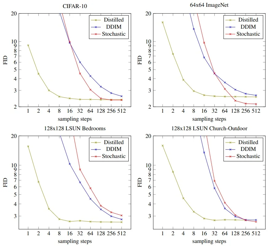
Key observations:
- On all datasets, the distilled model converges to comparable or better FID than DDIM with only a fraction of the steps.
- In unconditional CIFAR-10, the distilled sampler with just \( 4 \) steps achieves FID ˜2.1 — competitive with 50–100 step DDIM samplers.
These results validate the intuition behind distillation: rather than relying on numerical integration of the reverse-time SDE or ODE, we amortize this trajectory into a fixed sampler that mimics the high-quality path. As a result, inference can proceed in as few as 4–8 steps — reducing cost by more than an order of magnitude without noticeable degradation in fidelity.
Stochastic vs. Deterministic Baselines. The experiments also include a tuned stochastic sampler, where variance schedules are optimized via log-scale interpolation between upper and lower bounds (following Nichol & Dhariwal, 2021). For each number of steps, the interpolation coefficient is manually tuned to yield the best results. Still, progressive distillation matches or outperforms these handcrafted alternatives — showing that learning to mimic a deterministic high-quality sampler is more effective than manually adjusting variance schedules.
Conclusion Progressive distillation transforms diffusion models from slow, high-fidelity samplers into efficient generative tools by compressing the sampling process into a small number of learned denoising steps. Rather than predicting noise in an unstable low-SNR regime, each distilled model learns to reproduce the behavior of a high-quality sampler using a fraction of the original steps. This amortized integration not only accelerates generation by orders of magnitude but does so without sacrificing sample quality — as evidenced across diverse datasets and resolutions. As a result, progressive distillation provides a principled, scalable solution to one of the most critical bottlenecks in diffusion-based generative modeling.
Enrichment 20.9.7: Noise Conditional Score Networks
DDPM and DDIM (Enrichments Enrichment 20.9.1 and 20.9.2.5.0) are usually taught as denoising processes that start from Gaussian noise and iteratively remove it. A closely related line of work reached a similar destination from the opposite direction: instead of learning how to denoise, it tried to learn a vector field that always points toward regions of high data density. This is the score-based perspective, and its most influential early instance is Noise Conditional Score Networks (NCSN) [601]. While later diffusion models proved easier to train and faster to sample from, NCSN is the missing conceptual link that motivates the continuous-time SDE viewpoint formalized by Song et al. [605]. We’ll cover it right after as it is a key milestone for more advanced works in the field.
The score viewpoint: eliminating the normalization constant For a probability density \(p(\mathbf {x})\) on \(\mathbb {R}^d\), the Stein score function (or simply “the score”) is defined as the gradient of the log-density with respect to the data: \begin {equation} \label {eq:chapter20_score_def} \mathbf {s}^\star (\mathbf {x}) \;=\; \nabla _{\mathbf {x}} \log p(\mathbf {x}). \end {equation} This definition contains a subtle but powerful property. If we write the density as an unnormalized energy model \(p(\mathbf {x}) = \frac {e^{-E(\mathbf {x})}}{Z}\), the logarithm decomposes into \(\log e^{-E(\mathbf {x})} - \log Z\). Since the partition function \(Z\) is constant with respect to \(\mathbf {x}\), its gradient is zero. Therefore, \(\mathbf {s}^\star (\mathbf {x}) = -\nabla _{\mathbf {x}} E(\mathbf {x})\). The score allows us to model the shape of the distribution without ever needing to compute the intractable normalization constant \(Z\).
Conceptually, the score defines a vector field over the entire input space. If we view probability density as elevation, the score is a compass pointing strictly uphill. Starting from a random point, we can generate samples by following these arrows via Langevin dynamics—a stochastic process that combines gradient ascent (to find modes) with injected noise (to explore the volume of the distribution and prevent collapsing to a single point). Thus, sampling reduces to a problem of learning this vector field.
The manifold hypothesis and the empty room If the score provides such a clean sampling mechanism, why can’t we simply train a network to estimate \(\nabla _{\mathbf {x}} \log p(\mathbf {x})\) on clean images? The failure of this naive approach stems from the geometry of high-dimensional data. According to the manifold hypothesis, natural images occupy a low-dimensional substructure (a manifold) embedded within the vast, high-dimensional pixel space.
Consider the “thread in a warehouse” analogy: the data distribution is a thin thread suspended in a massive, empty room. The score is well-defined on the thread, but if we initialize the Langevin process with random noise, we start somewhere in the empty void of the room. In these empty regions, the true density \(p(\mathbf {x})\) is effectively zero, and the log-density is flat or numerically undefined. Consequently, the gradient \(\nabla _{\mathbf {x}} \log p(\mathbf {x})\) vanishes or becomes random noise. Without a meaningful signal to guide the random walker toward the manifold, the sampling process fails to converge. This “score estimation gap” in ambient space is the primary obstacle NCSN aims to solve.
To solve the empty room problem, Song and Ermon proposed thickening the data manifold by perturbing it with Gaussian noise at various scales \(\sigma \). Mathematically, we replace the singular data distribution with a mixture of Gaussians: \begin {equation} \label {eq:chapter20_mollified_density} p_\sigma (\mathbf {x}) \;=\; \int p_{\mbox{data}}(\mathbf {x}_0)\, \mathcal {N}(\mathbf {x};\,\mathbf {x}_0,\sigma ^2\mathbf {I})\,d\mathbf {x}_0. \end {equation} This operation fundamentally changes the geometry of the problem. Where the original density \(p_{\mbox{data}}\) was zero almost everywhere, the perturbed density \(p_\sigma \) is non-zero everywhere (it has full support). The ”fog” of probability now fills the entire room, meaning the log-density is mathematically well-defined at every point in space.
The score as a vector field pointing home Why do we care about the gradient of this foggy distribution? Consider a single data point \(\mathbf {x}_0\) perturbed by noise to create \(\tilde {\mathbf {x}} \sim \mathcal {N}(\mathbf {x}_0, \sigma ^2 \mathbf {I})\). For a Gaussian, the gradient of the log-density is linear: \begin {equation} \nabla _{\tilde {\mathbf {x}}} \log \mathcal {N}(\tilde {\mathbf {x}}; \mathbf {x}_0, \sigma ^2 \mathbf {I}) \;=\; -\frac {\tilde {\mathbf {x}} - \mathbf {x}_0}{\sigma ^2} \;\propto \; (\mathbf {x}_0 - \tilde {\mathbf {x}}). \end {equation} This is the crucial intuition: The score vector points directly from the noisy point \(\tilde {\mathbf {x}}\) back toward the clean data \(\mathbf {x}_0\). By learning the score of the perturbed distribution \(\nabla _{\mathbf {x}} \log p_\sigma (\mathbf {x})\), we are effectively learning a vector field that acts as a ”homing signal”, telling us how to move from any random point in space back toward the high-density data manifold.
The Dilemma: Reach vs. Precision A single noise level forces a devastating trade-off between the ”reach” of the gradient and the precision of the sample.
- High Noise (Large \(\sigma \)): The distribution is a giant, blurry blob. The gradients are powerful and long-range—they can guide a point from the far corners of the input space toward the center of the data mass. However, they lack all high-frequency detail. A gradient at this scale might tell you ”this is a face”, but it cannot distinguish between eyes and a mouth.
- Low Noise (Small \(\sigma \)): The distribution is sharp and detailed. The gradients contain perfect information about texture and edges. However, they are effectively myopic; they vanish just a few units away from the manifold. If the sampler isn’t already standing right next to a valid image, the gradient is zero (or random noise), and the process gets lost in the void.
The Solution: A Ladder of Noise Scales NCSN solves this by employing a sequence of noise scales \(\sigma _1 > \sigma _2 > \dots > \sigma _L\), effectively creating a hierarchy of distributions that bridges the gap between pure noise and the clean data manifold.
Think of this like finding a specific house on a digital map. At the start (high noise \(\sigma _1\)), you are zoomed out to the global view. You can’t see the house, but you can easily find the correct city. As you reduce the noise (\(\sigma _2, \sigma _3\dots \)), you essentially ”zoom in”. You find the neighborhood, then the street, and finally the specific address. You cannot start zoomed in (small \(\sigma \)) because you wouldn’t know which city to look in; you cannot stay zoomed out (large \(\sigma \)) because you’d never find the front door.
The Protocol: Mixing and Handing Off The crucial innovation in NCSN is not just having the scales, but how we traverse them. We do not simply slide down the noise levels. At each rung of the ladder \(\sigma _i\), we stop and perform a series of Langevin MCMC updates (typically \(K\) steps).
These steps allow the process to ”mix”—to settle into the typical set of the current distribution \(p_{\sigma _i}\). Effectively, we establish a ”base camp” at the current level of detail before attempting to move to the next. Once the sampler has converged to the coarse structure of \(\sigma _i\), we use its final position as the initialization for the next scale \(\sigma _{i+1}\).
This handoff ensures that when we switch to a lower noise level (where the gradients are shorter-range), we are guaranteed to be within the ”basin of attraction” of the manifold. We progressively position ourselves closer and closer to the data, ensuring that the gradient signal is always valid and points in the right direction.
The intractable marginal vs. the simple training target Our ultimate goal is to learn the score of the entire data distribution, \(\nabla _{\tilde {\mathbf {x}}}\log p_\sigma (\tilde {\mathbf {x}})\). Computing this directly is impossible because it requires summing the gradient contributions from every image in the dataset simultaneously—an intractable integration.
However, during training, we have a ”cheat code”. We create the noisy data ourselves! In every training step, we take a specific clean image \(\mathbf {x}_0\), add noise \(\sigma \boldsymbol {\epsilon }\), and generate a noisy input \(\tilde {\mathbf {x}}\). Because we know exactly which \(\mathbf {x}_0\) and \(\boldsymbol {\epsilon }\) we used, we can compute the conditional score—the gradient pointing back to this specific instance: \begin {equation} \label {eq:chapter20_conditional_score} \nabla _{\tilde {\mathbf {x}}}\log p(\tilde {\mathbf {x}} \mid \mathbf {x}_0) \;=\; -\frac {\tilde {\mathbf {x}}-\mathbf {x}_0}{\sigma ^2} \;=\; -\frac {\boldsymbol {\epsilon }}{\sigma }. \end {equation} This term acts as a precise ”homing signal”, telling us exactly where the clean data \(\mathbf {x}_0\) lies relative to the noisy observation.
Using the conditional score as a loss function We use this simple vector \(-\frac {\boldsymbol {\epsilon }}{\sigma }\) as the target label for a noise-conditional score network. Concretely, we train \(\mathbf {s}_\theta (\tilde {\mathbf {x}}, \sigma )\) to regress to the conditional score by minimizing \begin {equation} \label {eq:chapter20_dsm_single_sigma} \mathcal {L}(\theta ;\sigma ) \;=\; \frac {1}{2}\, \mathbb {E}_{\mathbf {x}_0\sim p_{\mbox{data}},\,\boldsymbol {\epsilon }\sim \mathcal {N}(\mathbf {0},\mathbf {I})} \left [ \left \| \mathbf {s}_\theta (\mathbf {x}_0+\sigma \boldsymbol {\epsilon },\sigma ) +\frac {\boldsymbol {\epsilon }}{\sigma } \right \|_2^2 \right ]. \end {equation} This turns the intractable marginal-score problem into standard supervised regression, repeated across noise scales.
Why does this work? (The ”Magic” of DSM) You might wonder: “If we train on instance-specific targets that point back to \(\mathbf {x}_0\), why doesn’t the network just memorize training images?”
The key is that the optimal regressor under squared loss is a conditional expectation. For a fixed noise level \(\sigma \), minimizing Equation 20.59 yields \[ \mathbf {s}_\theta ^\star (\tilde {\mathbf {x}},\sigma ) \;=\; \mathbb {E}\!\left [ -\frac {\boldsymbol {\epsilon }}{\sigma } \;\middle |\; \tilde {\mathbf {x}}=\mathbf {x}_0+\sigma \boldsymbol {\epsilon } \right ]. \] Vincent [667] shows that this conditional expectation is exactly the marginal score \(\nabla _{\tilde {\mathbf {x}}}\log p_\sigma (\tilde {\mathbf {x}})\). Intuitively, each noisy input \(\tilde {\mathbf {x}}\) is compatible with many underlying clean images; the regression solution therefore averages the “point-back” directions in a way that recovers the true gradient of the \(\sigma \)-perturbed density. In this precise sense, denoising and score matching coincide.
Training a Unified Score Network Rather than training a separate neural network for every noise level (which would be computationally prohibitive), NCSN [601] trains a single noise-conditional model \(\mathbf {s}_\theta (\mathbf {x}, \sigma )\).
The architecture is typically a U-Net, but with a crucial modification: the noise level \(\sigma \) is not just an input channel. Instead, it is injected into every layer of the network using Conditional Normalization (such as Conditional Instance Normalization or AdaGN).
The network predicts the score for any given \(\sigma \) by modulating its internal feature statistics—effectively, the scalar \(\sigma \) acts as a ”context switch” that tells the network whether it should be looking for coarse global shapes or fine-grained textures.
The training objective aggregates the Denoising Score Matching loss across all scales \(\sigma \in \{\sigma _1, \dots , \sigma _L\}\): \begin {equation} \label {eq:chapter20_ncsn_objective} \mathcal {L}(\theta ) \;=\; \mathbb {E}_{\mathbf {x}_0, \boldsymbol {\epsilon }, \sigma } \left [ \lambda (\sigma )\, \underbrace { \left \| \mathbf {s}_\theta (\mathbf {x}_0+\sigma \boldsymbol {\epsilon },\sigma ) - \left ( -\frac {\boldsymbol {\epsilon }}{\sigma } \right ) \right \|_2^2 }_{\mbox{Squared error w.r.t. target score}} \right ]. \end {equation}
Balancing the ”Screaming” and the ”Whispering” The weighting term \(\lambda (\sigma )\) is the most critical hyperparameter for convergence. To understand why, look at the magnitude of the target vector: \(\|\mathbf {s}^*\| \propto 1/\sigma \).
- Small \(\sigma \) (Fine details): The target vectors are massive (since we divide by a tiny number). The loss for these terms is naturally huge—the fine details are effectively ”screaming” at the optimizer.
- Large \(\sigma \) (Global structure): The target vectors are tiny. These terms contribute almost nothing to the raw unweighted loss—the global structure is merely ”whispering”.
If we set \(\lambda (\sigma )=1\), the optimizer effectively ignores the global structure to focus entirely on minimizing the massive error at small noise levels. The result would be a model that generates perfect textures but incoherent global shapes.
Song and Ermon proposed setting \(\lambda (\sigma ) = \sigma ^2\). Since the squared norm of the target scales as \(1/\sigma ^2\), multiplying by \(\sigma ^2\) cancels this factor out. This ensures that every noise scale contributes roughly equally (order \(O(1)\)) to the total gradient, forcing the network to learn both the global composition and the fine details simultaneously.
Sampling via Annealed Langevin Dynamics Once the score network \(\mathbf {s}_\theta (\mathbf {x}, \sigma )\) is trained, generation becomes an iterative process of refining random noise into a structured image. We cannot simply follow the score field deterministically from random initialization: a pure gradient flow typically converges to a mode (often a poor proxy for the full distribution) and does not produce diverse samples. To sample from the distribution rather than optimize toward a mode, we use Langevin dynamics, which injects noise at every step so the trajectory can explore the typical set instead of collapsing to a single basin.
NCSN employs Annealed Langevin Dynamics, which functions like a relay race across the noise ladder \(\sigma _1 > \sigma _2 > \dots > \sigma _L\). We initialize \(\mathbf {x}_0\) from a broad prior (pure noise) and run \(K\) steps of updates at each noise level before handing the state off to the next level.
The update rule at step \(k\) for noise level \(\sigma _i\) is: \begin {equation} \label {eq:chapter20_annealed_langevin} \mathbf {x}_{k+1} \;=\; \mathbf {x}_k + \underbrace {\frac {\eta _i}{2}\,\mathbf {s}_\theta (\mathbf {x}_k,\sigma _i)}_{\mbox{Gradient Force}} + \underbrace {\sqrt {\eta _i}\,\mathbf {z}_k}_{\mbox{Langevin Noise}}, \qquad \mathbf {z}_k\sim \mathcal {N}(\mathbf {0},\mathbf {I}). \end {equation} Here, \(\eta _i\) is the step size. Crucially, we scale the step size with the noise level, typically setting \(\eta _i \propto \sigma _i^2\). This ensures the Signal-to-Noise Ratio (SNR) remains constant: as the noise scales down, our steps become smaller and more precise to avoid overshooting the fine details.
The Protocol: Mixing and Handing Off You might ask: why not just take one step at \(\sigma _1\), then one at \(\sigma _2\), and so on? The reason is that we need to position ourselves correctly before the rules of the game change.
At a high noise level \(\sigma _1\), the energy landscape is smooth and the ”basins of attraction” are huge. By taking \(K\) steps (where \(K\) is often 100 or more), we allow the Langevin process to ”mix” or ”thermalize”—effectively letting the sample wander around until it finds the high-probability region (the ”typical set”) of the coarse distribution.
We are essentially establishing a ”base camp” in the rough vicinity of a valid image. Only once the sample has settled into this region is it safe to lower the noise to \(\sigma _2\). If we switched scales too quickly, the sample might still be in a low-probability region (a ”dead zone”) relative to the sharper \(\sigma _2\) distribution, where the gradients might be misleading or vanishing.
The ”Sculpting” Analogy Think of this process as sculpting a statue from a block of marble.
- High \(\sigma \) (Chiseling): We use a large hammer and chisel (large steps). We knock off huge chunks of rock to reveal the rough silhouette of a figure. We strike many times (multiple steps) until the general form is established.
- Low \(\sigma \) (Polishing): We switch to fine files and sandpaper (small steps). We work on the eyelids, the fingers, and the texture of the skin. At this stage, a large strike would ruin the statue; we need gentle, precise updates to refine the details established in the previous phase.
The ”Grand Unification”: A Hint of What’s Next NCSN was a pivotal moment in generative modeling because it proved that score matching could scale to high-dimensional images. However, its sampling algorithm (Annealed Langevin) felt remarkably similar to the reverse diffusion process of DDPM, yet the two methods used completely different mathematical derivations.
- NCSN viewed generation as moving through a ladder of noise scales with increasing variance (Variance Exploding).
- DDPM viewed generation as reversing a markov chain while keeping variance bounded (Variance Preserving).
The true power of this perspective is unlocked when we ask: ”What happens if we add more steps to the noise ladder until the space between them vanishes?”. Song et al. [605] showed that in the limit of infinite steps (\(L \to \infty \)), both the discrete noise ladder of NCSN and the Markov chain of DDPM converge to the same mathematical object: a Stochastic Differential Equation (SDE).
This insight changes the game entirely. Once generation is framed as solving a differential equation driven by a learned vector field, we can stop inventing ad-hoc update rules like Equation 20.61. Instead, we can treat sampling as a problem of numerical integration, allowing us to use powerful off-the-shelf solvers (like Runge-Kutta) to traverse the probability landscape with unprecedented speed and precision. This unification is the subject of the next section.
Enrichment 20.9.8: Score Based Generative Modeling with SDEs
Enrichment Enrichment 20.9.6 presented NCSN as a practical recipe: learn a noise-conditional score field and then sample using annealed Langevin dynamics. Song et al. [605] show that this recipe and the DDPM/DDIM viewpoints are not separate ideas, but merely different discretizations of a single continuous-time picture.
The profound consequence of this unification is that it separates the model (the differential equation) from the sampling algorithm (the solver).
Before the SDE perspective, researchers had to invent specific, rigid ”update rules” for generation. For example, NCSN required a carefully tuned schedule of step sizes and noise levels; DDPM required a specific formula to move from \(t\) to \(t-1\). If you wanted to speed up sampling, you had to re-derive the math and invent a new rule.
With the SDE formulation, sampling becomes a standard numerical simulation problem. Given a forward SDE, Song et al. [605] derive the corresponding reverse-time SDE, which we simulate using general-purpose SDE solvers (e.g., Euler–Maruyama or stochastic Runge–Kutta). They also show that the same family of marginals can be generated by a deterministic probability flow ODE, which can be integrated by black-box ODE solvers (e.g., adaptive Runge–Kutta), often reducing the number of score evaluations substantially. In short: the model is the continuous-time dynamics, and the sampler is the numerical solver used to integrate it.
The Continuum Limit: From Discrete Steps to Continuous Flow Up to this point, our notation followed the discrete DDPM setup: we indexed corruption by integers \(i \in \{0, \dots , N\}\). To pass to a continuous-time viewpoint, we separate these roles:
- Let \(N\) be the number of discrete steps (the grid resolution).
- Let \(T>0\) be the terminal time of the process (often \(T=1\)).
We introduce a time grid \(0=t_0 < t_1 < \dots < t_N=T\) and interpret discrete states as samples of a trajectory: ... \(\mathbf {x}_i \approx \mathbf {x}(t_i)\). As we refine this grid (\(N \to \infty \)), the discrete updates converge (in an appropriate sense) to a continuous-time stochastic process governed by an Itô Stochastic Differential Equation (SDE):
\begin {equation} \label {eq:chapter20_forward_sde_generic} d\mathbf {x} \;=\; \underbrace {\mathbf {f}(\mathbf {x},t)\,dt}_{\mbox{Drift (Deterministic)}} \;+\; \underbrace {g(t)\,d\mathbf {w}}_{\mbox{Diffusion (Random)}}, \qquad t\in [0,T], \end {equation} where \(\mathbf {w}\) is a standard Wiener process.
To build intuition, consider a tiny step \(\Delta t\): \[ \mathbf {x}(t+\Delta t) \;\approx \; \mathbf {x}(t) \;+\; \underbrace {\mathbf {f}(\mathbf {x}(t),t)\,\Delta t}_{\mbox{Deterministic } O(\Delta t)} \;+\; \underbrace {g(t)\,\sqrt {\Delta t}\,\mathbf {z}}_{\mbox{Stochastic } O(\sqrt {\Delta t})}, \qquad \mathbf {z}\sim \mathcal {N}(\mathbf {0},\mathbf {I}). \]
Why ”Drift” and ”Diffusion”?
- Drift (\(\mathbf {f}\)): the systematic component of the dynamics—it determines the mean infinitesimal change, scaling as \(O(\Delta t)\). For VP-type diffusions, the drift includes a restoring term that counteracts the injected noise and keeps the process bounded.
- Diffusion (\(g\)): the random component driven by Brownian motion. The stochastic increment has variance proportional to \(\Delta t\), so its typical magnitude scales as \(O(\sqrt {\Delta t})\), producing the characteristic “rough” trajectories of diffusion processes.
How is this derived? The forward SDE is typically derived by taking the limit of a Markov chain. As we increase the number of steps \(N \to \infty \), we ensure the total amount of noise added remains constant by making each individual step \(\Delta t\) infinitesimally small. By matching the first two moments (mean and variance) of the discrete update rule to the drift and diffusion coefficients, we ensure that the SDE’s marginal distributions \(p_t(\mathbf {x})\) converge to the discrete levels of the original model.
Ultimately, specifying \(\mathbf {f}\) and \(g\) defines the model (how data is corrupted), while the choice of solver defines the algorithm used to simulate it [605].
Two Canonical Families: VE and VP The SDE framework of Song et al. [605] makes the unification concrete: once we specify a forward corruption SDE \(\,d\mathbf {x}=\mathbf {f}(\mathbf {x},t)\,dt+g(t)\,d\mathbf {w}\,\), the entire family of sampling procedures (DDPM-style stochastic sampling, DDIM-style deterministic sampling, and predictor–corrector hybrids) becomes a question of how we numerically integrate the corresponding reverse-time dynamics. Two canonical forward processes cover the historical “branches” of the literature:
- Variance Exploding (VE): corrupt by only adding noise, so the conditional variance grows from near-zero to very large.
- Variance Preserving (VP): corrupt by shrinking + adding noise, so the overall scale stays bounded (and can be kept near unit variance).
To avoid notational ambiguity with the earlier discrete DDPM presentation (where \(\mathbf {x}_T\) meant the maximally noised state after \(T\) discrete steps), we will be explicit here: continuous time is \(t\in [0,T]\) (often \(T=1\)), and \(\mathbf {x}(t)\) denotes the state at time \(t\). A discretization uses a grid \(0=t_0<t_1<\cdots <t_N=T\) with \(\Delta t=t_i-t_{i-1}\), and we write \(\mathbf {x}_i \approx \mathbf {x}(t_i)\). In the special case where we match the earlier DDPM notation, \(\mathbf {x}_T\) corresponds to \(\mathbf {x}(T)\) (maximally noised), while \(\mathbf {x}_0\) corresponds to \(\mathbf {x}(0)\) (clean data).
1. Variance Exploding (VE-SDE) \(\leftrightarrow \) NCSN/SMLD In the NCSN/SMLD line, one specifies a noise scale schedule \(\sigma (t)\) that increases from \(\sigma (0)\approx 0\) to a large \(\sigma (T)=\sigma _{\max }\). The forward corruption keeps the signal unscaled and injects progressively larger Gaussian noise. A clean way to see the connection is to start from the discrete perturbation viewpoint.
-
Discrete viewpoint (“Adding the Missing Variance”)
In the Variance Exploding (VE) framework, we define an increasing sequence of noise scales \(\sigma _1 < \sigma _2 < \dots < \sigma _L\). Our goal is to ensure that at any step \(i\), the image is a corrupted version of the clean data \(\mathbf {x}_0\) such that: \[ \mathbf {x}_i \mid \mathbf {x}_0 \sim \mathcal {N}(\mathbf {x}_0, \sigma _i^2 \mathbf {I}). \]Suppose we are currently at step \(i-1\) with variance \(\sigma _{i-1}^2\). To reach the next variance level \(\sigma _i^2\), we must add exactly enough fresh Gaussian noise to bridge the gap. Since variances add linearly (\(\mbox{Var}(A+B) = \mbox{Var}(A) + \mbox{Var}(B)\)), we solve for the “missing” variance: \[ \sigma _i^2 = \sigma _{i-1}^2 + \mbox{Var}(\mbox{noise}) \implies \mbox{Var}(\mbox{noise}) = \sigma _i^2 - \sigma _{i-1}^2. \]
This gives us the discrete update rule: \begin {equation} \label {eq:chapter20_ve_discrete_increment} \mathbf {x}_i \;=\; \mathbf {x}_{i-1} + \underbrace {\sqrt {\sigma _i^2 - \sigma _{i-1}^2}\,\mathbf {z}_i}_{\mbox{The Variance Gap}}, \qquad \mathbf {z}_i \sim \mathcal {N}(\mathbf {0}, \mathbf {I}). \end {equation}
Intuition: Notice that \(\mathbf {x}_{i-1}\) is multiplied by \(1\). Unlike DDPM, there is no multiplicative shrinkage on the signal. The clean image \(\mathbf {x}_0\) remains the mean of the distribution forever; it just gets increasingly buried under a mounting pile of noise.
-
Continuous-time limit (Diffusion-only SDE)
To transition to continuous time, we view the discrete levels as samples from a smooth function \(\sigma (t)\). As the step size \(\Delta t \to 0\), the discrete variance increment \(\sigma (t_i)^2 - \sigma (t_{i-1})^2 \) becomes the differential \(d[\sigma ^2(t)]\). Using the chain rule: \[ d[\sigma ^2(t)] \approx \frac {d[\sigma ^2(t)]}{dt} \Delta t. \]We need to match this to the standard SDE form \(d\mathbf {x} = g(t)d\mathbf {w}\). Recall that the variance of a Brownian increment \(d\mathbf {w}\) is simply \(dt\). Therefore, the variance contributed by the SDE is \(g^2(t) dt\). Setting these equal: \[ g^2(t) dt = \frac {d[\sigma ^2(t)]}{dt} dt \implies g(t) = \sqrt {\frac {d[\sigma ^2(t)]}{dt}}. \]
Since there is no scaling of the signal in the discrete rule, the deterministic drift \(\mathbf {f}(\mathbf {x}, t)\) is zero. This yields the diffusion-only SDE: \begin {equation} \label {eq:chapter20_ve_sde} d\mathbf {x} \;=\; \underbrace {\sqrt {\frac {d[\sigma ^2(t)]}{dt}}}_{g(t)}\,d\mathbf {w}, \qquad t \in [0, T]. \end {equation} This equation tells us that the ”speed” of our diffusion is determined entirely by the instantaneous rate at which we want the noise variance to grow.
The corresponding marginal is especially transparent: because the forward VE process only adds zero-mean noise, it preserves the mean and increases variance according to \(\sigma ^2(t)\): \begin {equation} \label {eq:chapter20_ve_marginal} \mathbf {x}(t)\mid \mathbf {x}(0) \;\sim \; \mathcal {N}\!\bigl (\mathbf {x}(0),\,\sigma ^2(t)\mathbf {I}\bigr ). \end {equation} Intuitively, VE can be read as a controlled decay of signal-to-noise ratio (SNR): the signal component stays put, while the noise radius expands until the sample becomes essentially indistinguishable from a wide Gaussian cloud.
2. Variance Preserving (VP-SDE) \(\leftrightarrow \) DDPM In the DDPM line, the forward process is designed so that the state remains bounded (and, under mild assumptions, close to unit variance). The familiar discrete forward chain \( \mathbf {x}_t=\sqrt {1-\beta _t}\,\mathbf {x}_{t-1}+\sqrt {\beta _t}\,\mathbf {z} \) is exactly an Euler–Maruyama discretization of the VP-SDE in the small-step limit.
- Discrete viewpoint (shrink + add). Each step slightly attenuates the current state and injects fresh Gaussian noise: \begin {equation} \label {eq:chapter20_vp_discrete} \mathbf {x}_i \;=\; \sqrt {1-\beta _i}\,\mathbf {x}_{i-1} + \sqrt {\beta _i}\,\mathbf {z}_i, \qquad \mathbf {z}_i\sim \mathcal {N}(\mathbf {0},\mathbf {I}). \end {equation} The attenuation prevents the trajectory from “blowing up”: the noise we add is continuously balanced by the energy we remove.
-
Continuous-time limit (Ornstein–Uhlenbeck type)
To derive the Variance Preserving SDE, we define a continuous noise rate \(\beta (t)\). For a very small time step \(\Delta t\), the discrete variance is \(\beta _t \approx \beta (t)\Delta t\).Let’s examine the discrete update \(\mathbf {x}_t = \sqrt {1-\beta _t}\mathbf {x}_{t-1} + \sqrt {\beta _t}\mathbf {z}\). To find the differential \(d\mathbf {x}\), we look at the change \(\Delta \mathbf {x} = \mathbf {x}_t - \mathbf {x}_{t-1}\): \[ \Delta \mathbf {x} = (\sqrt {1-\beta (t)\Delta t} - 1)\mathbf {x}_{t-1} + \sqrt {\beta (t)\Delta t}\mathbf {z}. \]
The Taylor Bridge: At the limit where \(\Delta t \to 0\), the term \(\beta (t)\Delta t\) becomes an infinitesimal \(u\). We use the first-order Taylor expansion: \[ \sqrt {1-u} \approx 1 - \frac {1}{2}u + \mathcal {O}(u^2). \] Substituting \(u = \beta (t)\Delta t\) back into our equation: \[ \Delta \mathbf {x} \approx \left ( (1 - \frac {1}{2}\beta (t)\Delta t) - 1 \right )\mathbf {x}_{t-1} + \sqrt {\beta (t)}\sqrt {\Delta t}\mathbf {z}. \]
Simplifying the terms, the \(1\) and \(-1\) cancel out, leaving: \[ \Delta \mathbf {x} \approx -\frac {1}{2}\beta (t)\mathbf {x}_{t-1}\Delta t + \sqrt {\beta (t)}(\sqrt {\Delta t}\mathbf {z}). \]
In the limit, \(\Delta t\) becomes the differential \(dt\), and the term \(\sqrt {\Delta t}\mathbf {z}\) becomes the Brownian increment \(d\mathbf {w}\) (since both represent a random variable with variance \(dt\)). This yields the VP-SDE: \begin {equation} \label {eq:chapter20_vp_sde} d\mathbf {x} \;=\; \underbrace {-\frac {1}{2}\beta (t)\,\mathbf {x}\,dt}_{\mbox{Drift (Deterministic)}} \;+\; \underbrace {\sqrt {\beta (t)}\,d\mathbf {w}}_{\mbox{Diffusion (Random)}}, \qquad t\in [0,T]. \end {equation}
Intuition: The “Thermostatted Spring”
This equation describes an Ornstein–Uhlenbeck process, a cornerstone of
statistical mechanics originally used to model the velocity of a particle under the
influence of friction and thermal fluctuations. In the context of diffusion, you can
think of it as a thermostatted spring:
- The Spring (Drift): The term \(-\frac {1}{2}\beta (t)\mathbf {x}\) acts like a spring attached to the origin. If a pixel value drifts too far (becoming very bright or very dark), the ”spring” pulls it back toward zero. This acts as a deterministic restoring force that prevents the signal energy from growing.
- The Thermal Kicks (Diffusion): The term \(\sqrt {\beta (t)}\,d\mathbf {w}\) represents random thermal fluctuations. These ”kicks” inject noise and push the particle away from the origin in random directions.
Crucially, as \(\beta (t)\) increases according to the noise schedule, we both pull harder and inject stronger noise simultaneously. This delicate balance is why the process is called “Variance Preserving”.
If the initial data is standardized such that \(\mathrm {Cov}(\mathbf {x}(0)) = \mathbf {I}\), the inward pull of the drift exactly counteracts the outward pressure of the diffusion. The result is a process where the covariance stays bounded at \(\mathbf {I}\) throughout time, ensuring the image remains within a stable numerical range rather than exploding.
The VP marginal takes the same affine form as the DDPM closed-form: \begin {equation} \label {eq:chapter20_vp_marginal} \mathbf {x}(t) \;=\; \alpha (t)\,\mathbf {x}(0) + \sqrt {1-\alpha ^2(t)}\,\boldsymbol {\epsilon }, \qquad \boldsymbol {\epsilon }\sim \mathcal {N}(\mathbf {0},\mathbf {I}), \end {equation} where the continuous-time shrinkage factor is: \begin {equation} \label {eq:chapter20_vp_alpha} \alpha (t) \;=\; \exp \!\left (-\frac {1}{2}\int _0^t \beta (s)\,ds\right ). \end {equation}
Why the Integral? The Calculus of Compounding You may wonder why the product of discrete terms \(\sqrt {1-\beta _t}\) transforms into an exponential integral. Recall that in DDPM, the cumulative scaling factor is the product \(\prod _{s=1}^t \sqrt {1-\beta _s}\).
If we take the natural logarithm of this product, it becomes a sum of logs: \[ \ln \left ( \prod \sqrt {1-\beta _s} \right ) = \sum \frac {1}{2} \ln (1-\beta _s). \] Using the Taylor approximation \(\ln (1-u) \approx -u\) for very small \(u\), and substituting \(\beta _s \approx \beta (s)ds\), the sum becomes a Riemann integral: \[ \sum \frac {1}{2} \ln (1-\beta _s) \approx \sum -\frac {1}{2}\beta (s)ds \longrightarrow -\frac {1}{2}\int _0^t \beta (s)ds. \] Exponentiating both sides brings us back to \(\alpha (t)\), as defined in Equation 20.69.
What is happening here? The integral \(\int _0^t \beta (s)ds\) represents the total accumulated noise pressure up to time \(t\). The exponential function then translates this total pressure into a scaling factor.
- When \(t=0\), the integral is 0, so \(\alpha (0) = e^0 = 1\). The signal is fully preserved.
- As \(t\) increases, the integral grows, causing \(\alpha (t)\) to decay toward 0. The signal is gradually ”shrunk” away.
This makes the ”Variance Preserving” (VP) name mathematically precise: as the signal \(\alpha (t)\mathbf {x}(0)\) shrinks, the noise term \(\sqrt {1-\alpha ^2(t)}\boldsymbol {\epsilon }\) grows in the exact proportion needed to keep the total variance of \(\mathbf {x}(t)\) equal to \(1\) (assuming unit variance data).
Reverse time dynamics and why the score appears The forward SDE defines a continuum of densities \(p_t(\mathbf {x})\) that evolve from data to noise. The generative direction runs backward from \(t=T\) to \(t=0\). A key theorem in Song et al. [605] shows that reversing this process modifies the drift by a term involving the score \(\nabla _{\mathbf {x}}\log p_t(\mathbf {x})\):
\begin {equation} \label {eq:chapter20_reverse_sde_generic} d\mathbf {x} \;=\; \Bigl [\mathbf {f}(\mathbf {x},t) - g^2(t)\,\nabla _{\mathbf {x}}\log p_t(\mathbf {x})\Bigr ]\,dt +\; g(t)\,d\bar {\mathbf {w}}, \qquad t\in [T,0]. \end {equation}
The score term is the “restoring vector field” pointing toward high-density regions. Training a score network \(\mathbf {s}_\theta (\mathbf {x},t)\approx \nabla _{\mathbf {x}}\log p_t(\mathbf {x})\) turns sampling into a simulation: plug \(\mathbf {s}_\theta \) into the reverse SDE and integrate back to \(t=0\).
Probability flow and the DDIM connection Song et al. further show that these marginals \(\{p_t\}\) can be realized by a deterministic ODE, obtained by adjusting the drift: \begin {equation} \label {eq:chapter20_probability_flow_ode} \frac {d\mathbf {x}}{dt} \;=\; \mathbf {f}(\mathbf {x},t) -\frac {1}{2}g^2(t)\,\mathbf {s}_\theta (\mathbf {x},t). \end {equation}
This probability flow ODE is the rigorous home for the DDIM phenomenon. DDPM is a discretization of the stochastic reverse SDE, while DDIM is a discretization of the deterministic ODE.
Why Unification Matters: The VE vs. VP Trade-off Viewing NCSN and DDPM as SDE choices reveals their different numerical burdens:
- 1.
- Scale management: VE grows \(\sigma (t)\) to massive values, requiring the model to be well-conditioned across orders of magnitude. VP uses restoring drift to keep the state bounded.
- 2.
- Solver behavior: Sampling becomes a problem of stiffness. Depending on the schedule, one family may admit larger stable steps (fewer function evaluations) than the other.
- 3.
- Numerical Analysis Shift: The “model” is the probability path, and the “sampler” is the choice of solver. We can now use 50 years of calculus research to generate images in a few steps instead of a\(~ 1000\).
This shift also clarifies the role of deterministic dynamics: the probability flow ODE provides a deterministic sampler that shares the same time-marginals as the stochastic diffusion. In principle, integrating the ODE forward yields a deterministic “encoding” of data into a latent noise variable, and integrating it backward decodes noise into data; in practice, the fidelity of such mappings depends on score-approximation and numerical-integration error. Ultimately, the central object is the learned score field: once we can estimate \(\nabla _{\mathbf {x}}\log p_t(\mathbf {x})\) across time, we can instantiate many different samplers by choosing how to integrate the associated reverse-time SDE or probability-flow ODE.
Predictor-Corrector Sampling The SDE view clarifies why Langevin refinement is not a separate idea, but a corrector interleaved with a predictor. A generic Predictor-Corrector (PC) sampler alternates:
- Predictor: Take one numerical step for the reverse SDE or ODE (moving from \(t_i\) to \(t_{i-1}\)).
- Corrector: At the fixed time \(t_{i-1}\), run Langevin MCMC to re-thermalize and pull the sample toward high-density regions.
# Predictor-Corrector sampling (conceptual)
x = sample_from_prior()  # x(T) ~ p_T
for i in reversed(range(1, N + 1)):
    t, t_prev = t_grid[i], t_grid[i - 1]
    dt = t_prev - t

    # 1) Predictor: one step of a reverse-time SDE solver or probability-flow ODE solver
    x = predictor_step(x, t, dt, score_model=s_theta)

    # 2) Corrector: Langevin refinement at fixed time t_prev
    for _ in range(M):
        grad = s_theta(x, t_prev)
        x = x + (eps / 2) * grad + math.sqrt(eps) * torch.randn_like(x)

return x  # approximate sample from p_0
The taxonomy is now unified: NCSN is corrector-heavy, DDPM is an SDE predictor, and DDIM is an ODE predictor.
From Theory to Practice: The Path to EDM Song et al. provided the ”grand unification”, but also exposed a massive design space. The theory gives us the equations, but not the engineering ”Golden Rules”: Which noise schedule is best? How should we parameterize the network? Which solvers work in a small number of steps?
The next section explores how Karras et al. systematically addressed these in Elucidating the Design Space of Diffusion-Based Generative Models (EDM), turning this theoretical unification into the most efficient generative framework to date.
Enrichment 20.9.9: Elucidating the Design Space of Diffusion Models (EDM)
The SDE framework of Song et al. [605] provides a rigorous mathematical map of diffusion, but it remains silent on the numerical reality of training: standard U-Nets are initialized and optimized for unit-variance inputs (\(\sigma \approx 1\)), yet the diffusion process requires noise levels as high as \(\sigma =80\) (variance \(\approx 6400\)). Feeding such raw scales into a network shatters optimization stability. Karras et al. [292] (EDM) resolve this paradox by strictly decoupling the physical SDE dynamics from the internal network operations. Their framework ensures the network only ever operates in a numerically ”comfortable” regime, regardless of whether the image is almost clean or pure noise. This is achieved via a three-part recipe:
- Pre-conditioning (The Numerical Shell): Instead of feeding raw noisy data into the U-Net, EDM wraps the network in a mathematical shell. This shell automatically scales every input down to unit variance (\(\approx 1\)) before it enters the first layer, and scales every output back up to the correct physical magnitude after it leaves. This prevents the network’s internal signals from exploding or vanishing.
- Loss Weighting (Gradient Equalization): At low noise levels, the network’s influence on the final image is naturally smaller. Without a correction, the ”learning signal” (gradients) for fine details would be so tiny that the optimizer would ignore them. EDM uses a \(\sigma \)-dependent weight that acts like an amplifier for these quiet signals, ensuring that learning fine textures at low noise is just as prioritized as learning global structure at high noise .
-
Sampling (Compute Reallocation): EDM treats the denoising process as a path through a curved space.
- Where the image changes most: At high noise levels, the image is just vague blobs that don’t change much with small steps. But at low noise levels (\(\sigma \approx 0\)), even tiny changes in \(\sigma \) result in massive shifts in sharpness and fine detail.
- The Fix: EDM uses a power-law schedule that takes a few massive steps at high noise and many tiny, precise steps at low noise. This ”spends” the compute budget where the visual complexity is highest.
Why naive continuous-time training fails The core pathology of continuous-time training is a massive dynamic-range mismatch. To understand the numerical challenge, we must contrast how different diffusion families handle variance:
- Variance Exploding (VE): Noise is strictly added (\(\mathbf {x} = \mathbf {x}_0 + \sigma \boldsymbol {\epsilon }\)). As \(\sigma \) increases toward the maximum (e.g., \(80\)), the input variance explodes to \(\approx 6400\), saturating the U-Net’s activations immediately.
- Variance Preserving (VP): In DDPM-style VP diffusion, the forward marginal is typically written as \[ \mathbf {x}_t \;=\; \alpha _t\,\mathbf {x}_0 \;+\; \sigma _t\,\boldsymbol {\epsilon }, \qquad \boldsymbol {\epsilon }\sim \mathcal {N}(\mathbf {0},\mathbf {I}), \qquad \alpha _t^2+\sigma _t^2=1, \] so the mixing coefficients are bounded even though the effective SNR varies dramatically. At late times \(\alpha _t\to 0\), the data term is strongly attenuated and the network must recover structure from a near unit-variance noise floor. (Importantly, \(\sigma _t\) here is a VP coefficient and should not be conflated with EDM’s continuous noise scale \(\sigma \) used in the additive model \(\mathbf {x}=\mathbf {x}_0+\sigma \boldsymbol {\epsilon }\) ).
Why standard normalization is not enough EDM’s starting point is that diffusion training exposes a single backbone to a continuum of noise levels. In the additive corruption view \(\mathbf {x}=\mathbf {x}_0+\sigma \boldsymbol {\epsilon }\) with \(\boldsymbol {\epsilon }\sim \mathcal {N}(\mathbf {0},\mathbf {I})\), the input scale is \[ \mathrm {Std}(\mathbf {x}) \;=\; \sqrt {\sigma _{\mbox{data}}^2+\sigma ^2}, \] so the raw magnitude presented to the first convolution varies by orders of magnitude across \(\sigma \).
A natural question is whether generic normalization layers (BatchNorm, GroupNorm, LayerNorm) can simply “absorb” this dynamic range. EDM’s answer is no: these mechanisms can stabilize intermediate activations, but they do not yield the \(\sigma \)-aware conditioning and first-layer protection that diffusion demands.
- 1.
- The first-layer conditioning problem is external. Most normalization acts after a learned linear transform. When \(\sigma \) is large, the first convolution receives inputs far outside the scale assumed by standard initializations, so the early pre-activations and their gradients are poorly conditioned before any internal normalization can intervene. Diffusion therefore needs an explicit, deterministic rescaling before the first layer.
- 2.
- Scale carries semantics in diffusion. The denoiser must implement qualitatively different behavior across \(\sigma \): at small \(\sigma \) it should be near an identity map (preserve already-correct pixels), while at large \(\sigma \) it must act as a strong prior (hallucinate global structure). Forcing partial scale-invariance via activation normalization discards physically meaningful magnitude information and pushes the network to reconstruct it indirectly through conditioning. In diffusion, the goal is not just “stable activations,” but stable numerics that preserve the meaning of scale.
- 3.
- BatchNorm is especially ill-posed. Diffusion training deliberately mixes a wide range of \(\sigma \) values across samples and minibatches, making the activation distribution strongly non-stationary. This undermines the running-statistics assumption that BatchNorm relies on.
EDM’s remedy is to move normalization outside the backbone and make it explicitly \(\sigma \)-aware. Concretely, EDM wraps a raw network \(F_\theta \) with analytic gates that (i) scale the input by \(c_{\mbox{in}}(\sigma )\) before the first layer, (ii) re-scale the learned correction by \(c_{\mbox{out}}(\sigma )\), and (iii) blend it with a skip path via \(c_{\mbox{skip}}(\sigma )\), while providing \(\sigma \) through an explicit noise embedding \(c_{\mbox{noise}}(\sigma )\). This guarantees that \(F_\theta \) always operates in a standardized numerical regime, while the dependence on noise level is preserved by the geometry of the wrapper rather than being normalized away.
From Noise-Prediction to Data-Prediction: The Logic of \(D_\theta \) Earlier models like DDPM primarily optimized the backbone to predict the noise component \(\boldsymbol {\epsilon }\). While this was suitable for stochastic Langevin dynamics, EDM treats generation as a deterministic path through an ODE. In this framework, training the network to be a direct denoiser \(D_\theta (\mathbf {x};\sigma )\)—predicting the clean image \(\mathbf {x}_0\) directly—offers a crucial mathematical anchor.
Even though generation is a multi-step process, this ”one-step” prediction serves as a reference point for the local dynamics at every iteration:
- The Anchor (Tweedie’s Formula): In a Gaussian corruption model, the network’s estimate of the clean signal \(\mathbf {x}_0\) is the bridge to the Score Function. Specifically, \(\nabla _{\mathbf {x}}\log p(\mathbf {x};\sigma ) = (D_\theta (\mathbf {x};\sigma ) - \mathbf {x}) / \sigma ^2\). By predicting the data instead of the noise, the network provides the exact vector field required to drive the Probability Flow ODE.
- Curvature Correction: Predicting \(\mathbf {x}_0\) allows the solver to estimate the ”final destination” at the current noise level. This is essential for higher-order solvers like Heun’s method: by comparing how the estimated \(\mathbf {x}_0\) (and thus the score) shifts between two points, the solver can account for the curvature of the trajectory, taking much larger steps than a simple noise-subtraction scheme would allow.
To make this direct prediction numerically stable, EDM requires a reference for the ”natural scale” of the signal, denoted as \(\sigma _{\mbox{data}}\). This is the standard deviation of the clean dataset (typically \(0.5\) for pixels normalized to \([-1,1]\)). Because the added noise is statistically independent of the image, the total variance of any noisy input \(\mathbf {x} = \mathbf {x}_0 + \sigma \boldsymbol {\epsilon }\) is simply the sum of the variances: \[ \mathrm {Var}(\mathbf {x}) \;=\; \underbrace {\sigma _{\mbox{data}}^2}_{\mbox{Signal Power}} \;+\; \underbrace {\sigma ^2}_{\mbox{Noise Power}}. \] This additivity is the numerical backbone of the framework. It provides an exact formula for the magnitude of \(\mathbf {x}\) at any noise level. Instead of forcing the network to ”learn” the current noise volume—a task that shifts by orders of magnitude—we use this formula to compute analytic scaling factors (\(c_{\mbox{in}}, c_{\mbox{out}}\)) that normalize the signals.
The network is thus freed from managing the dynamic range (the volume) and can focus entirely on the geometry (the structure). By decoupling the numerical scale of the diffusion process from the internal operations of the U-Net, EDM ensures the weights always face a standardized, unit-variance problem. This makes the learning process significantly more consistent, whether the image is buried under \(0.1\) or \(80\) units of noise.
Pre-conditioning as fixed gates around a raw network Instead of asking a raw U-Net \(F_\theta \) to learn across wildly varying magnitudes, EDM decouples the physical signal scale from the network’s internal numerics. It defines the denoiser as a \(\sigma \)-dependent wrapper that forces the neural network to operate in a ”unit-variance” regime at all times: \begin {equation} \label {eq:chapter20_edm_precond_wrapper} D_\theta (\mathbf {x};\sigma ) \;=\; \underbrace {c_{\mbox{skip}}(\sigma )\,\mathbf {x}}_{\mbox{Linear Pass-through}} \;+\; \underbrace {c_{\mbox{out}}(\sigma )\,F_\theta \!\bigl (\underbrace {c_{\mbox{in}}(\sigma )\,\mathbf {x}}_{\mbox{Normalized Input}};\;c_{\mbox{noise}}(\sigma )\bigr )}_{\mbox{Neural Correction}}. \end {equation} These coefficients behave like fixed gates that control the flow of signal and noise. They are not learned parameters, but analytic functions derived strictly from the variance statistics of the noise schedule. Using the data scale \(\sigma _{\mbox{data}}\) (typically \(0.5\)), the ”golden” EDM scalings are: \begin {align} \label {eq:chapter20_edm_coeffs} c_{\text {in}}(\sigma ) &= \frac {1}{\sqrt {\sigma ^2+\sigma _{\text {data}}^2}}, & c_{\text {noise}}(\sigma ) &= \frac {1}{4}\ln \sigma , \\ c_{\text {skip}}(\sigma ) &= \frac {\sigma _{\text {data}}^2}{\sigma ^2+\sigma _{\text {data}}^2}, & c_{\text {out}}(\sigma ) &= \frac {\sigma \,\sigma _{\text {data}}}{\sqrt {\sigma ^2+\sigma _{\text {data}}^2}}. \end {align}
The Logic of the Gates: \(\sigma \) as the Physical Coordinate Unlike standard models that index the process by an abstract time variable \(t \in [0, 1]\), EDM treats the noise level \(\sigma \) itself as the independent variable. In this ”time-free” framework, the input \(\mathbf {x}\) is seen as a physical mixture of data and noise at a specific scale \(\sigma \).
By treating \(\sigma \) as the primary coordinate, the design of these coefficients shifts from ”scheduling” to Variance Equalization. During the inference loop, the sampler chooses a sequence of \(\sigma \) values (the ”schedule”) and provides them to the wrapper.
Each gate then acts as an analytic function that adjusts the Signal-to-Noise Ratio (SNR) for that specific scale, ensuring the backbone always operates in a unit-variance regime:
- Input Gate \(c_{\mbox{in}}(\sigma )\) (The Gain Control): During inference, as the image becomes cleaner, the total variance of the input \(\mathbf {x}\) drops. \(c_{\mbox{in}}\) scales the input inversely to its standard deviation \(\sqrt {\sigma ^2+\sigma _{\mbox{data}}^2}\). This ensures the U-Net always receives a ”normalized” image, preventing the internal weights from having to adapt to shifting input magnitudes at different steps of the schedule.
- Skip Gate \(c_{\mbox{skip}}(\sigma )\) (The Signal-to-Noise Crossfader): This gate manages the ”trust” between the raw noisy input and the network’s correction. At the start of inference (\(\sigma \approx 80\)), the input is pure noise; \(c_{\mbox{skip}}\) is near \(0\), forcing the system to rely entirely on the neural prediction. As we reach the final steps of inference (\(\sigma \to 0\)), the input is almost clean; \(c_{\mbox{skip}}\) approaches \(1.0\), effectively ”shielding” the already-correct pixels from unnecessary neural alteration.
- Output Gate \(c_{\mbox{out}}(\sigma )\) (The Magnitude Restorer): The internal network (\(F_\theta \)) is trained to output a ”shape-only” update at unit variance. \(c_{\mbox{out}}\) re-scales this update to the physical magnitude required by the current \(\sigma \). Mathematically, it is coupled with \(c_{\mbox{in}}\) to equalize the gradient scale, ensuring that a 1% correction is just as effective at the beginning of inference as it is at the end.
- Noise Embedding \(c_{\mbox{noise}}(\sigma )\) (The Logarithmic Eye): The network is told ”where it is” in the process through a logarithmic mapping \(\frac {1}{4}\ln \sigma \). This ensures that the sampler’s exponential steps (e.g., jumping from \(\sigma =80\) to \(40\)) are presented to the network as linear transitions. This mapping allows the network’s embedding layers to interpolate smoothly between vastly different noise scales.
Inference Flow: How values are chosen How does the system know which \(\sigma \) values to feed the gates during generation? This is determined by the discretization schedule. In standard models, we might take 50 equal steps from \(t=1\) to \(0\). EDM recognizes that the image doesn’t change linearly. Instead, it uses the power-law schedule (defined later on) to choose \(\sigma \) values.
At the start of inference, the solver takes large jumps in \(\sigma \) (e.g., \(80 \to 50 \to 30\)) because at high noise levels, the ”velocity” of the image formation is relatively constant. As we approach \(\sigma =0\), the schedule dictates tiny, precise steps (e.g., \(0.1 \to 0.05 \to 0.02\)). At each of these points, the solver queries the network: ”Given the current image at noise \(\sigma _i\), what is the clean \(\mathbf {x}_0\)?” The gates use that specific \(\sigma _i\) value to normalize the numbers, the network makes its guess, and the solver uses that guess to calculate the next step in the schedule.
Implementation: The EDM Wrapper In practice, this analytic shell is implemented as a lightweight module wrapping the backbone.
def forward(self, x, sigma):
    # x: [Batch, Channels, H, W]
    # sigma: [Batch] (must be broadcastable to x)

    # 1. Compute variances
    # sigma_data is usually 0.5
    var_data = self.sigma_data ** 2
    var_noise = sigma ** 2
    total_std = (var_data + var_noise).sqrt()

    # 2. Compute the analytic gates
    c_skip = var_data / (var_data + var_noise)
    c_out = (sigma * self.sigma_data) / total_std
    c_in = 1.0 / total_std
    c_noise = sigma.log() / 4.0

    # 3. Apply the wrapper
    # The inner model F_theta never sees the raw variance explosion
    F_x = self.inner_model(c_in * x, c_noise)
    D_x = c_skip * x + c_out * F_x

    return D_x
A \(\sigma \)-balanced loss: Equalizing gradients via inverse weighting Once the denoiser \(D_\theta \) is wrapped to control input variance, we must ensure the gradients flowing back from the loss function are equally well-behaved. EDM trains using a weighted Euclidean distance to the clean image \(\mathbf {x}_0\): \begin {equation} \label {eq:chapter20_edm_loss} \mathcal {L}_{\mbox{EDM}} \;=\; \mathbb {E}_{\mathbf {x}_0,\boldsymbol {\epsilon },\sigma } \left [ \lambda (\sigma )\, \underbrace {\left \lVert D_\theta (\mathbf {x}_0+\sigma \boldsymbol {\epsilon };\sigma ) - \mathbf {x}_0 \right \rVert _2^2}_{\mbox{Raw Squared Error}} \right ]. \end {equation} The raw error term is problematic because \(D_\theta \) scales its output by \(c_{\mbox{out}}(\sigma )\). The subtle issue is not that \(c_{\mbox{out}}(\sigma )\) explodes at large \(\sigma \) (in EDM it is bounded by \(\sigma _{\mbox{data}}\)), but that \(c_{\mbox{out}}(\sigma )\to 0\) as \(\sigma \to 0\). Because the learnable branch enters as \(c_{\mbox{out}}(\sigma )\,F_\theta (\cdot )\), the gradient signal that reaches the raw network weights is proportional to \(c_{\mbox{out}}(\sigma )\) (while the skip term \(c_{\mbox{skip}}(\sigma )\mathbf {x}\) is non-learned).
With an unweighted loss, small-noise examples would therefore contribute vanishingly little learning signal, making it difficult to learn fine textures and edges.
EDM chooses \(\lambda (\sigma )\) so that the effective coefficient \(\lambda (\sigma )\,c_{\mbox{out}}^2(\sigma )\) is (approximately) constant, equalizing gradient magnitudes over the full noise range. The optimal weighting is the inverse square of the output scaler: \begin {equation} \label {eq:chapter20_edm_lambda} \lambda (\sigma ) \;=\; \frac {1}{c_{\mbox{out}}^2(\sigma )} \;=\; \frac {\sigma ^2+\sigma _{\mbox{data}}^2}{(\sigma \,\sigma _{\mbox{data}})^2}. \end {equation}
Why this works (The ”Whitening” Effect): Recall that the denoiser output is roughly \(c_{\mbox{out}} \cdot F_\theta \). By weighing the loss by \(1/c_{\mbox{out}}^2\), we effectively strip away the outer wrapper’s scaling from the optimization objective: \[ \lambda (\sigma ) \cdot \lVert D_\theta - \mathbf {x}_0 \rVert ^2 \;\approx \; \frac {1}{c_{\mbox{out}}^2} \cdot \lVert c_{\mbox{out}} F_\theta - \dots \rVert ^2 \;\approx \; \lVert F_\theta - \mbox{target} \rVert ^2. \] This ensures that the internal network \(F_\theta \) sees a ”unit-variance” loss landscape. The contribution of a training example to the gradient depends only on the difficulty of the sample, not on the arbitrary magnitude of \(\sigma \), preventing the optimization from becoming myopic to specific frequency bands.
From denoiser to sampling: the EDM ODE in noise-level coordinates EDM frames sampling as integrating a probability-flow ODE whose independent variable can be chosen to be the noise standard deviation itself. In the canonical EDM choice \(\sigma (t)=t\) and \(s(t)=1\), the ODE takes the particularly transparent form \begin {equation} \label {eq:chapter20_edm_ode_sigma} \frac {d\mathbf {x}}{d\sigma } \;=\; \frac {\mathbf {x} - D_\theta (\mathbf {x};\sigma )}{\sigma }, \end {equation} where \(D_\theta (\mathbf {x};\sigma )\) denotes the network’s estimate of the clean image at noise level \(\sigma \).
Why this form is useful (“one-step denoise” as an Euler limit). If we were to take a single Euler step from \(\sigma \) directly to \(0\), we would obtain \[ \mathbf {x}(0) \;\approx \; \mathbf {x} \;+\; (0-\sigma )\,\frac {\mathbf {x}-D_\theta (\mathbf {x};\sigma )}{\sigma } \;=\; D_\theta (\mathbf {x};\sigma ), \] so \(D_\theta \) can be read as the endpoint suggested by the local ODE geometry at that noise level. This is exactly why higher-order solvers (e.g., Heun) improve fidelity: they correct the drift incurred by following only the initial tangent direction over a finite step.
For convenience in the sampler discussion below, define the ODE slope (velocity) as \[ \mathbf {d}(\mathbf {x},\sigma ) \;=\; \frac {\mathbf {x}-D_\theta (\mathbf {x};\sigma )}{\sigma }. \]
Heun’s method: Curvature correction via looking ahead Sampling involves integrating the ODE from \(\sigma _{\max }\) to \(0\). However, the probability flow trajectory is curved, not straight. A simple first-order Euler step (\(\mathbf {x}_{i+1} = \mathbf {x}_i + h \mathbf {d}_i\)) blindly follows the tangent at the starting point. By the time it arrives at the next noise level, the true manifold has curved away, leading to accumulation of error (drift).
EDM employs Heun’s Method (a 2nd-order predictor-corrector) to fix this. It ”looks ahead” to see how the curve bends before committing to a step. Let the ODE slope (velocity) at any point be: \[ \mathbf {d}(\mathbf {x},\sigma ) \;=\; \frac {\mathbf {x} - D_\theta (\mathbf {x};\sigma )}{\sigma }. \]
For a step from \(\sigma _i\) to \(\sigma _{i+1}\) (where step size \(h_i = \sigma _{i+1} - \sigma _i < 0\)), the process has two distinct stages:
- 1.
- The Predictor (Euler Guess): We take a tentative Euler step to estimate where we might land. \begin {equation} \label {eq:chapter20_edm_heun_predictor} \underbrace {\hat {\mathbf {x}}_{i+1}}_{\mbox{Candidate}} \;=\; \mathbf {x}_i \;+\; h_i \cdot \mathbf {d}(\mathbf {x}_i,\sigma _i). \end {equation}
- 2.
- The Corrector (Trapezoidal Refinement): We evaluate the slope at
that candidate point to see how the vector field has changed. Then, we
average the starting slope and the ending slope to find a better
direction:
\begin {align} \mathbf {d}_{\text {start}} &= \mathbf {d}(\mathbf {x}_i,\sigma _i), \\ \mathbf {d}_{\text {end}} &= \mathbf {d}(\hat {\mathbf {x}}_{i+1},\sigma _{i+1}), \\ \label {eq:chapter20_edm_heun_corrector} \mathbf {x}_{i+1} \;=\; \mathbf {x}_i \;+\; h_i \cdot \underbrace {\frac {\mathbf {d}_{\text {start}} + \mathbf {d}_{\text {end}}}{2}}_{\text {Average Slope}}. \end {align}
Geometric Intuition: Imagine driving a car along a curving road in the dark.
- Euler is like locking the steering wheel straight based on the road right in front of you. You will inevitably drive off the curve.
- Heun is like projecting where that straight line goes, seeing that the road curves left up ahead, and adjusting your steering angle to the average of ”straight” and ”left”.
This simple averaging (Trapezoidal Rule) cancels out the leading-order error term, allowing EDM to take much larger steps (e.g., \(N=35\)) without drifting off the data manifold.
Power-law noise schedule: Allocating compute where it counts The difficulty of the ODE integration is not uniform across time. The vector field changes character dramatically as \(\sigma \) drops:
- At High Noise (\(\sigma \gg 1\)): The image is just vague blobs. The denoiser’s target changes slowly, meaning the ODE path is relatively straight. We can afford to take massive steps here.
- At Low Noise (\(\sigma \approx 0\)): The image is crystallizing fine textures and sharp edges. The vector field varies rapidly with even tiny changes in \(\sigma \). If we step too fast here, we will introduce blurring or artifacts.
To address this, EDM abandons linear time steps. Instead, it defines a non-uniform discretization that heavily concentrates steps near \(\sigma =0\). This is achieved by mapping the noise levels into a ”linearized” space using an exponent \(\rho \) (typically \(\rho =7\)).
Let \(N\) be the total step budget. We perform linear interpolation between \(\sigma _{\max }^{1/\rho }\) and \(\sigma _{\min }^{1/\rho }\), and then map the result back to the original domain:
\begin {equation} \label {eq:chapter20_edm_powerlaw_schedule} \sigma _i \;=\; \left ( \sigma _{\max }^{1/\rho } \;+\; \frac {i}{N-1} \left ( \sigma _{\min }^{1/\rho }-\sigma _{\max }^{1/\rho } \right ) \right )^{\rho }, \qquad i=0,\dots ,N-1, \qquad \sigma _N = 0. \end {equation}
The Effect (\(\rho =7\)): This high exponent creates a drastic skew. For the typical EDM hyperparameters \(\sigma _{\min }=0.002\), \(\sigma _{\max }=80\), and \(\rho =7\), the midpoint \(i=(N-1)/2\) corresponds to \(\sigma \approx 2.5\), so roughly half of the solver evaluations occur below a few units of \(\sigma \)—precisely the range where perceptually important fine details emerge and the ODE curvature matters most.
Optional Churn: Stochastic error correction While the ODE solver is deterministic, discretization errors can cause the trajectory to drift off the true data manifold, especially with few steps. EDM introduces ”Churn” to mitigate this. It is effectively a partial Langevin MCMC step: we temporarily increase the noise level (moving backward up the schedule) and then let the ODE solver denoise it back down. This ”zig-zag” movement shakes the sample back toward high-probability regions, correcting minor drifts.
The process works by inflating the current noise level \(\sigma _i\) to a target \(\hat {\sigma }_i\) using a relative factor \(\gamma _i\). This injection is controlled by a set of explicit hyperparameters:
- \(S_{\mbox{churn}}\): The overall ”volatility” or amount of stochasticity to add per step.
- \(S_{\min }, S_{\max }\): The noise range where churn is active (typically applied only in the middle of the schedule, avoiding the delicate final details).
- \(S_{\mbox{noise}}\): A multiplier for the standard deviation of the injected noise (usually \(1.007\)).
The Algorithm: First, we calculate the inflation factor \(\gamma _i\), ensuring it doesn’t exceed theoretical stability limits (\(\sqrt {2}-1\)): \[ \gamma _i \;=\; \begin {cases} \min \!\left (\frac {S_{\mbox{churn}}}{N},\sqrt {2}-1\right ), & \mbox{if } \sigma _i \in [S_{\min }, S_{\max }], \\ 0, & \mbox{otherwise}. \end {cases} \] Then, we define the inflated noise level \(\hat {\sigma }_i = \sigma _i(1+\gamma _i)\) and physically inject random noise \(\boldsymbol {\epsilon }\) into the state \(\mathbf {x}_i\): \[ \hat {\mathbf {x}}_i \;=\; \mathbf {x}_i \;+\; \underbrace {\sqrt {\hat {\sigma }_i^2 - \sigma _i^2}}_{\mbox{Added Variance}} \cdot S_{\mbox{noise}} \cdot \boldsymbol {\epsilon }, \qquad \boldsymbol {\epsilon }\sim \mathcal {N}(\mathbf {0},\mathbf {I}). \] Finally, the ODE solver takes a step from the new inflated level \(\hat {\sigma }_i\) down to the next target \(\sigma _{i+1}\). Because \(\hat {\sigma }_i > \sigma _i\), the solver is forced to take a slightly larger step than usual to get back on track, effectively ”re-solving” the local structure with fresh randomness.
Reference pseudo-code for EDM sampling
def edm_sample(D, sigma_min, sigma_max, N, rho=7,
               S_churn=0.0, S_min=0.0, S_max=float("inf"), S_noise=1.0):
    """
    D(x, sigma): returns denoised prediction D_theta(x; sigma)
    sigmas[0] = sigma_max, sigmas[N] = 0
    """

    # Power-law schedule in sigma^{1/rho}, then exponentiate back.
    sigmas = []
    for i in range(N):
        u = sigma_max**(1.0/rho) + (i/(N-1))*(sigma_min**(1.0/rho) - sigma_max**(1.0/rho))
        sigmas.append(u**rho)
    sigmas.append(0.0)

    x = torch.randn_like(...) * sigma_max  # x_0 ~ N(0, sigma_max^2 I)

    for i in range(N):
        sigma_i, sigma_next = sigmas[i], sigmas[i+1]

        # Churn factor gamma_i (bounded by sqrt(2)-1), active only in [S_min, S_max]
        gamma = 0.0
        if S_min <= sigma_i <= S_max:
            gamma = min(S_churn / N, math.sqrt(2.0) - 1.0)

        # Temporarily increase noise level: sigma_hat = sigma_i * (1 + gamma)
        sigma_hat = sigma_i * (1.0 + gamma)

        # Inject noise to move from sigma_i to sigma_hat:
        # epsilon_i ~ N(0, S_noise^2 I)
        if gamma > 0.0:
            eps = torch.randn_like(x) * S_noise
            x_hat = x + (sigma_hat**2 - sigma_i**2).sqrt() * eps
        else:
            x_hat = x

        # Euler step from sigma_hat to sigma_next using the ODE slope
        d = (x_hat - D(x_hat, sigma_hat)) / sigma_hat
        x_next = x_hat + (sigma_next - sigma_hat) * d

        # Heun (2nd-order) correction, skipped at sigma_next = 0
        if sigma_next != 0:
            d_next = (x_next - D(x_next, sigma_next)) / sigma_next
            x_next = x_hat + (sigma_next - sigma_hat) * 0.5 * (d + d_next)

        x = x_next

    return x  # approximate sample at sigma = 0
Looking ahead: The transition to Velocity-space (\(v\)-prediction) EDM transformed diffusion from a fragile academic curiosity into a robust engineering pipeline. However, its rigorous analysis of scaling revealed a deeper lesson: numerical stability depends entirely on what the network is asked to predict. While EDM chooses to predict the clean image \(\mathbf {x}_0\), this choice creates a ”curved” trajectory in latent space that remains difficult to solve at extremely low step counts.
To overcome this, modern architectures, especially those designed for Progressive Distillation, move beyond predicting pixels or noise. They instead predict a velocity-style quantity \(\mathbf {v}_t\).
The velocity \(v\) is defined as a linear combination of the signal and the noise: \[ \mathbf {v}_t = \alpha _t \boldsymbol {\epsilon } - \sigma _t \mathbf {x}_0 \] By learning in this ”\(v\)-space”, the network effectively learns to follow a ”shorter”, more linear path from noise to data. This parameterization is not just a trick for stability; it is the fundamental requirement for Progressive Distillation, where we recursively ”distill” the knowledge of a many-step ODE solver into a few-step student model. Without the scale-invariant properties of velocity prediction, these distilled models would suffer from the same ”magnitude shift” errors that EDM’s pre-conditioning first identified. The next enrichment will explore how \(v\)-prediction serves as the mathematical engine for high-speed, few-step generation.
Enrichment 20.9.10: Velocity-Space Sampling: The Stability Bridge
Building on the insights from EDM [292], we can reframe diffusion as a continuous trajectory integrated via numerical solvers. This dramatically reduces the number of function evaluations needed for high-quality sampling. However, once we move toward ultra-fast sampling—using tens of steps rather than hundreds—a second, more subtle issue becomes dominant: the training target itself becomes ill-conditioned at the extremes of the noise schedule.
This subsection introduces velocity (\(v\)) prediction, a concept that originally emerged from the work on Progressive Distillation by Salimans and Ho [559]. While originally designed to facilitate the iterative ”halving” of sampling steps during distillation, \(v\)-prediction serves as a crucial stability bridge. It moves us away from the classical \(\boldsymbol {\epsilon }\)-prediction (DDPM) and toward a more robust representation that remains well-behaved even as the signal-to-noise ratio vanishes.
This shift is more than a numerical trick; it provides our first look at a vector-field viewpoint. This perspective—where we predict the direction and speed of the data-to-noise transformation—will culminate in the next section: Flow Matching, a powerful generalization that decouples the learning of the velocity field from the specific constraints of the diffusion corruption process.
Setup We begin with the standard reparameterized forward process, which defines the marginal distribution \(q(\mathbf {z}_t|\mathbf {x}_0)\) at any time \(t \in [0, 1]\): \begin {equation} \label {eq:chapter20_vspace_forward_reparam} \mathbf {z}_t = \alpha _t \mathbf {x}_0 + \sigma _t \boldsymbol {\epsilon }, \qquad \boldsymbol {\epsilon } \sim \mathcal {N}(\mathbf {0}, \mathbf {I}) \end {equation} where \(\alpha _t\) and \(\sigma _t\) are differentiable signal and noise scale. For the variance-preserving (VP) models discussed here, these are typically chosen such that \(\alpha _t^2 + \sigma _t^2 = 1\). Training proceeds by learning a denoising model \(\hat {\mathbf {x}}_\theta (\mathbf {z}_t)\) to estimate the original data, which is often implemented by predicting the noise \(\boldsymbol {\epsilon }\) via a network \(\hat {\boldsymbol {\epsilon }}_\theta (\mathbf {z}_t, t)\).
Crucially, this single training objective supports two fundamentally different sampling paradigms:
- Stochastic Sampling (DDPM): Following the original ancestral sampling rule, these models inject fresh Gaussian noise at each reverse step. This stochasticity allows the model to ”correct” its trajectory, but often requires hundreds of steps for high-quality results.
- Deterministic Sampling (DDIM / Probability Flow): Alternatively, one can treat sampling as solving a Probability Flow ODE. This defines a deterministic mapping from noise to data. While the individual sample paths are smooth and deterministic, they are mathematically constructed to share the same marginal distributions \(p_t(\mathbf {z})\) as the stochastic SDE.
Why naive \(\boldsymbol {\epsilon }\) prediction fails at the schedule boundaries Standard \(\boldsymbol {\epsilon }\)-prediction is not equally difficult across all timesteps; rather, it becomes numerically brittle exactly where we most need stability for fast sampling.
- 1.
- High-noise limit (\(t\approx 1\)) and error amplification
When \(t \to 1\), \(\alpha _t \to 0\) and the latent \(\mathbf {z}_t\) converges toward pure Gaussian noise. While predicting \(\boldsymbol {\epsilon }\) appears ”easy” (since the signal is mostly noise), the implied reconstruction of the original data becomes mathematically ill-conditioned: \begin {equation} \label {eq:vspace_x0_from_eps} \hat {\mathbf {x}}_\theta (\mathbf {z}_t) = \frac {\mathbf {z}_t - \sigma _t \hat {\boldsymbol {\epsilon }}_\theta (\mathbf {z}_t)}{\alpha _t}. \end {equation} Because this formula divides by \(\alpha _t\), any microscopic network error \(\boldsymbol {\delta } := \hat {\boldsymbol {\epsilon }}_\theta (\mathbf {z}_t,t)-\boldsymbol {\epsilon }\) is amplified when translated into an \(x_0\) estimate: \begin {equation} \label {eq:vspace_error_amp} \hat {\mathbf {x}}_{0,\theta }(\mathbf {z}_t,t) - \mathbf {x}_0 \;=\; -\frac {\sigma _t}{\alpha _t}\,\boldsymbol {\delta } \;=\; -\sqrt {\mathrm {SNR}(t)^{-1}}\;\boldsymbol {\delta }, \qquad \mathrm {SNR}(t):=\frac {\alpha _t^2}{\sigma _t^2}. \end {equation} As the signal vanishes (\(\alpha _t \to 0\)) in the high-noise regime, the scaling factor \(\sigma _t/\alpha _t\) (or \(\sqrt {\mathrm {SNR}(t)^{-1}}\)) diverges to infinity. Consequently, any microscopic network error \(\boldsymbol {\delta }\) is catastrophically magnified when translated into the \(\mathbf {x}_0\) estimate. While high-step samplers can iteratively ”correct” these early missteps, few-step distilled samplers lack this corrective capacity. In the distilled regime, this single amplified error becomes terminal, leading to the characteristic structural collapse or ”color shifting” often observed in low-fidelity samples. - 2.
- Loss Weighting and the SNR Imbalance (\(t \approx 0\))
A key fact is that the standard \(\boldsymbol {\epsilon }\)-MSE objective induces an SNR-weighted reconstruction objective in \(x_0\)-space. Starting from \(L_\theta =\mathbb {E}\bigl [\|\boldsymbol {\epsilon }-\hat {\boldsymbol {\epsilon }}_\theta (\mathbf {z}_t,t)\|_2^2\bigr ]\) and using \(\hat {\mathbf {x}}_{0,\theta }=(\mathbf {z}_t-\sigma _t\hat {\boldsymbol {\epsilon }}_\theta )/\alpha _t\), we obtain the exact identity \begin {equation} \|\boldsymbol {\epsilon }-\hat {\boldsymbol {\epsilon }}_\theta \|_2^2 \;=\; \frac {\alpha _t^2}{\sigma _t^2}\;\|\mathbf {x}_0-\hat {\mathbf {x}}_{0,\theta }\|_2^2 \;=\; \mathrm {SNR}(t)\,\|\mathbf {x}_0-\hat {\mathbf {x}}_{0,\theta }\|_2^2, \qquad \mathrm {SNR}(t):=\frac {\alpha _t^2}{\sigma _t^2}. \end {equation} Consequently, as \(t\to 1\) we have \(\mathrm {SNR}(t)\to 0\) and the high-noise regime receives vanishing weight, while as \(t\to 0\) we have \(\mathrm {SNR}(t)\to \infty \) and the low-noise regime dominates the gradients. This imbalance is often tolerable with many reverse steps (errors can be corrected gradually), but it becomes a major failure mode for ultra-fast sampling and progressive distillation, where the model must get the global trajectory right with very few chances to recover.The result is a model that ”perfects the grain of the wood while forgetting how to build the house”. For distillation to succeed, the model requires a parameterization—such as the \(\mathbf {v}\)-prediction or \(\mathbf {x}\)-prediction—that remains stable across this entire SNR range.
Velocity prediction as a bounded target To resolve the boundary pathologies of \(\boldsymbol {\epsilon }\)-prediction, Salimans and Ho [559] introduce the velocity (\(v\)) parameterization. This target is specifically designed to remain numerically stable across the entire noise schedule, a property that is critical for the success of few-step progressive distillation. We define the velocity target as a linear combination of the noise and the data:
\begin {equation} \label {eq:chapter20_vspace_vdef} \mathbf {v}_t \;:=\; \alpha _t\,\boldsymbol {\epsilon } - \sigma _t\,\mathbf {x}_0. \end {equation}
The geometric intuition here is profound. When using a variance-preserving schedule where \(\alpha _t^2 + \sigma _t^2 = 1\), the relationship between our latents (\(\mathbf {z}_t, \mathbf {v}_t\)) and our base variables (\(\mathbf {x}_0, \boldsymbol {\epsilon }\)) is an orthonormal rotation in the \((\mathbf {x}_0, \boldsymbol {\epsilon })\) plane: \[ \begin {bmatrix} \mathbf {z}_t \\[3pt] \mathbf {v}_t \end {bmatrix} = \begin {bmatrix} \alpha _t & \sigma _t \\ -\sigma _t & \alpha _t \end {bmatrix} \begin {bmatrix} \mathbf {x}_0 \\[3pt] \boldsymbol {\epsilon } \end {bmatrix}. \]
By framing \(v\) as a rotation, we gain several intuitive advantages:
- Norm Preservation: Since the transformation matrix is orthogonal, the combined ”energy” of the system is preserved. Because \(\mathbf {x}_0\) and \(\boldsymbol {\epsilon }\) are typically standardized, the target \(\mathbf {v}_t\) naturally stays on a comparable scale to the latent \(\mathbf {z}_t\) across the entire schedule.
- Angular Uniformity: Instead of dealing with exploding noise-to-signal ratios, we can view the diffusion process as a steady rotation along a circular arc from the data axis to the noise axis.
- Stability at the Limits: Unlike \(\epsilon \)-prediction, where the link to \(x\)-prediction breaks down at \(\alpha _t=0\), \(v\)-prediction remains a well-defined target. In fact, at the high-noise limit (\(\alpha _t \to 0\)), \(\mathbf {v}_t \approx -\mathbf {x}_0\), and at the low-noise limit (\(\sigma _t \to 0\)), \(\mathbf {v}_t \approx \boldsymbol {\epsilon }\).
Why this fixes the boundary pathologies Velocity prediction acts as an automatic, well-conditioned ”interpolator” between the two difficult extremes of the noise schedule:
- High-noise limit \((\alpha _t \to 0, \sigma _t \to 1)\): In this regime, \(\mathbf {v}_t \approx -\mathbf {x}_0\). Instead of the network attempting a fragile ”divide-by-zero” reconstruction of the image from a noise estimate, the target directly asks for data-aligned structure. This shift from identifying a residual to predicting an endpoint fundamentally stabilizes global composition in few-step sampling.
- Low-noise limit \((\alpha _t \to 1, \sigma _t \to 0)\): Here, \(\mathbf {v}_t \approx \boldsymbol {\epsilon }\). The target smoothly transitions to a noise-removal task where local denoising is the appropriate objective. Crucially, the learning problem remains well-scaled because \(\mathbf {v}_t\) is defined through an orthonormal rotation; it never inherits the \(\sigma _t/\alpha _t\) error amplification that plagues \(\epsilon \)-prediction.
Invertibility and practical decoding formulas A major practical advantage of \(v\)-prediction is its seamless compatibility with existing diffusion infrastructure. Because it is simply a change of basis, we can recover the estimated clean data (\(\hat {\mathbf {x}}_0\)) or the estimated noise (\(\hat {\boldsymbol {\epsilon }}\)) from the predicted velocity \(\hat {\mathbf {v}}_\theta (\mathbf {z}_t, t)\) using stable affine transformations: \begin {equation} \label {eq:chapter20_vspace_inversion} \hat {\mathbf {x}}_0 = \alpha _t \mathbf {z}_t - \sigma _t \hat {\mathbf {v}}_\theta (\mathbf {z}_t, t), \qquad \hat {\boldsymbol {\epsilon }} = \sigma _t \mathbf {z}_t + \alpha _t \hat {\mathbf {v}}_\theta (\mathbf {z}_t, t). \end {equation} These identities follow directly from the rotation interpretation and the requirement that \(\alpha _t^2 + \sigma _t^2 = 1\). It is important to view \(v\)-prediction not as a new model class, but as a numerically robust coordinate system for representing the same fundamental denoising information. This stability is what allows distilled models to collapse thousands of steps into a single, high-fidelity mapping.
Training objective The most direct way to train a \(v\)-parameterized model is by minimizing the Mean Squared Error (MSE) in velocity space: \begin {equation} \label {eq:chapter20_vspace_loss} \mathcal {L}_v(\theta ) = \mathbb {E}_{\mathbf {x}_0,\boldsymbol {\epsilon },t} \Bigl [ \|\hat {\mathbf {v}}_\theta (\mathbf {z}_t,t)-\mathbf {v}_t\|_2^2 \Bigr ], \qquad \mathbf {z}_t = \alpha _t\mathbf {x}_0 + \sigma _t\boldsymbol {\epsilon }. \end {equation} This loss can be justified as a weighted variational lower bound on the data log-likelihood.
Conceptually, this marks a pivotal shift in the diffusion narrative: we are no longer merely predicting a static noise latent (\(\boldsymbol {\epsilon }\)) or a distant endpoint (\(\mathbf {x}_0\)). Instead, the network learns to predict a directional vector field that is intrinsically aligned with the geometry of the Probability Flow ODE.
Mathematically, minimizing the \(v\)-MSE loss is equivalent to an \(x\)-space reconstruction loss with a unique, time-dependent weighting: \begin {equation} \label {eq:chapter20_vspace_loss_equivalence} \|\hat {\mathbf {v}}_\theta -\mathbf {v}_t\|_2^2 \;=\; \frac {1}{\sigma _t^2}\,\|\hat {\mathbf {x}}_{0,\theta }-\mathbf {x}_0\|_2^2 \;=\; \bigl (1+\mathrm {SNR}(t)\bigr )\,\|\hat {\mathbf {x}}_{0,\theta }-\mathbf {x}_0\|_2^2, \qquad (\alpha _t^2+\sigma _t^2=1). \end {equation} By adding \(1\) to the signal-to-noise ratio, this objective ensures that the model receives a non-vanishing gradient even at the highest noise levels where the SNR approaches zero.
This “SNR\(+1\)” weighting provides a more balanced multi-task learning signal, preventing the optimization from being dominated solely by the low-noise regime where the standard \(\epsilon \)-loss weighting would otherwise vanish.
Implementation sketch The only change relative to \(\boldsymbol {\epsilon }\)-prediction is the target computation and the decoding formulas:
# v-parameterization training (conceptual)
# Given: clean batch x0, timestep t, schedule alpha_t, sigma_t
eps = torch.randn_like(x0)
xt = alpha_t * x0 + sigma_t * eps

v_target = alpha_t * eps - sigma_t * x0
v_pred = v_net(xt, t)               # predicts v

loss = ((v_pred - v_target) ** 2).mean()

# optional: decode x0 or eps if needed
x0_hat = alpha_t * xt - sigma_t * v_pred
eps_hat = sigma_t * xt + alpha_t * v_pred
Bridge to multi-task optimization While velocity prediction (\(\mathbf {v}\)-space) solves the parameterization problem by keeping training targets well-scaled at both trajectory ends, it does not fully resolve the fundamental multi-task nature of diffusion training. One might assume that frameworks like EDM, which prioritize sampling steps in high-SNR regimes to refine detail, would naturally mitigate imbalance; however, the training objective itself remains vulnerable to gradient domination.
The core issue lies in the relationship between sampling density and optimization priority. While we sample more often at high-SNR to polish textures, the standard reconstruction loss implicitly weights these steps by the SNR itself: \(w(\lambda _t) = \mbox{SNR}(t)\). At the low-noise limit (\(t \to 0\)), the SNR blows up to infinity. This creates a ”gradient tyranny” where the model over-prioritizes microscopic residual patterns while assigning near-zero importance to the high-noise steps that define global composition.
To restore this balance, we introduce the Min-SNR-\(\gamma \) weighting strategy [210] next. Importantly, the precise weight depends on the chosen parameterization. For a \(v\)-parameterized objective, a convenient form is \begin {equation} \label {eq:vspace_minsnr} w_t^{(v)} \;=\; \frac {\min \{\mathrm {SNR}(t),\gamma \}}{\mathrm {SNR}(t)+1}, \qquad \mathrm {SNR}(t)=\frac {\alpha _t^2}{\sigma _t^2}, \end {equation} so that multiplying \(w_t^{(v)}\) by the intrinsic \((\mathrm {SNR}(t)+1)\) factor of the \(v\)-MSE yields an effective \(x_0\)-space weight of \(\min \{\mathrm {SNR}(t),\gamma \}\), preventing the low-noise regime from dominating optimization.
By capping the weight at \(\gamma \), we prevent the optimization from becoming ”obsessed” with high-frequency textures that it cannot distinguish from noise. This ensures the network maintains the modeling capacity required to build the structural ”foundation” of the image at \(t \approx 1\). We now proceed to explain the implementation of Min-SNR-\(\gamma \) in detail before transitioning to the Flow Matching paradigm, which cleanly decouples velocity field learning from the specific corruption mechanics of diffusion.
Enrichment 20.9.11: Min-SNR-\(\gamma \): Loss Reweighting as Multi-Task Balancing
Numerical stabilizers such as EDM-style preconditioning and \(v\)-prediction fix the immediate numerical brittleness of diffusion training by ensuring targets do not explode or vanish at schedule boundaries. However, these parameterizations do not resolve the underlying multi-task learning pathology. Even with stable targets, diffusion training involves solving a continuum of distinct denoising tasks. In modern frameworks like EDM, these tasks are indexed directly by the continuous noise standard deviation \(\sigma \), rather than an arbitrary timestep \(t\), and the network is conditioned explicitly on \(\sigma \).
These tasks do not contribute equally to the learning process; Hang et al. [210] identify that a primary bottleneck is negative transfer—a phenomenon where the optimization direction for one task conflicts with another. Crucially, this manifests as a gradient dominance problem within the mini-batch. During training, a batch contains samples corrupted at various noise levels. In standard formulations, the implicit loss weighting scales with the Signal-to-Noise Ratio (\(\mathrm {SNR}\)). Consequently, samples drawn from the low-noise (high-SNR) regime produce gradients with massive magnitudes, while samples from the high-noise (low-SNR) regime produce gradients with negligible magnitudes. When these per-sample gradients are averaged to update the weights, the low-noise samples—which only teach texture refinement—hijack the optimization direction, effectively drowning out the signal from high-noise samples responsible for learning global structure.
Their proposed Min-SNR-\(\gamma \) strategy resolves this conflict by enforcing a Pareto-stationary weighting scheme: it explicitly clamps the per-sample loss weight for high-SNR inputs. This prevents the ”easy” texture tasks from monopolizing the gradient budget, ensuring that the optimizer remains responsive to the structural errors found in the high-noise regime.
Diffusion training as many tasks sharing one network Consider the reparameterized forward process. While early formulations indexed this process by discrete timesteps \(t\), modern frameworks like EDM [292] emphasize that the fundamental coordinate is the continuous noise level \(\sigma \). We can write the generalized transition as:
\begin {equation} \label {eq:chapter20_forward_reparam} \mathbf {x}_\sigma \;=\; c_{\mbox{signal}}(\sigma )\,\mathbf {x}_0 \;+\; c_{\mbox{noise}}(\sigma )\,\boldsymbol {\epsilon }, \qquad \boldsymbol {\epsilon } \sim \mathcal {N}(\mathbf {0}, \mathbf {I}), \end {equation} where \(c_{\mbox{signal}}\) and \(c_{\mbox{noise}}\) determine the schedule (e.g., \(c_{\mbox{signal}}=\alpha _t, c_{\mbox{noise}}=\sigma _t\) in VP-diffusion; \(c_{\mbox{signal}}=1, c_{\mbox{noise}}=\sigma \) in EDM’s VE-diffusion). For any fixed noise level \(\sigma \), the network is asked to solve a distinct inverse problem:
- Low SNR (High \(\sigma \)): The input is dominated by noise. The model must perform generation, inferring global structure and semantic composition from minimal signal.
- High SNR (Low \(\sigma \)): The input is nearly clean. The model must perform restoration, removing microscopic residual noise without over-smoothing fine textures.
These objectives are qualitatively different, yet their gradients are pooled into a single set of network parameters. Empirical analysis reveals that optimizing for specific noise levels can harm performance on distant ones (negative transfer). If the training loss implicitly over-emphasizes the high-SNR tasks, the model exhausts its capacity polishing imperceptible details while undertraining the low-SNR steps that determine global composition.
Why Gradient Clipping is Insufficient One might assume that standard gradient clipping—a technique ubiquitous in deep learning—would resolve these imbalances by preventing the high-SNR gradients from exploding. However, clipping operates on the global gradient vector \(\mathbf {g}_{\mbox{total}} = \sum _\sigma w_\sigma \mathbf {g}_\sigma \). If the high-SNR components \(\mathbf {g}_{\mbox{high}}\) dominate this sum due to excessive weighting \(w_{\mbox{high}}\), the direction of \(\mathbf {g}_{\mbox{total}}\) aligns almost exclusively with \(\mathbf {g}_{\mbox{high}}\). Gradient clipping scales the magnitude of this vector (\(\mathbf {g} \leftarrow \mathbf {g} \cdot \min (1, C/\|\mathbf {g}\|)\)) but strictly preserves its direction. Consequently, the update remains biased toward texture refinement at the expense of structural generation, regardless of the clipping threshold. Min-SNR-\(\gamma \) addresses the root cause by rebalancing the weights \(w_\sigma \) themselves, ensuring the aggregate gradient vector represents a directional compromise between all denoising tasks.
Why naive uniform weighting fails The fundamental diagnostic is that being “uniform in \(t\)” (sampling timesteps with equal probability) does not imply that all noise levels contribute equally to learning. The imbalance enters through the implicit weighting induced by the chosen prediction target.
To make this precise, we work in the standard VP reparameterization: \begin {equation} \label {eq:chapter20_minsnr_vp_reparam} \mathbf {z}_t \;=\; \alpha _t \mathbf {x}_0 \;+\; \sigma _t \boldsymbol {\epsilon }, \qquad \boldsymbol {\epsilon }\sim \mathcal {N}(\mathbf {0},\mathbf {I}), \qquad \alpha _t^2+\sigma _t^2=1, \end {equation} and define the (dimensionless) Signal-to-Noise Ratio \begin {equation} \label {eq:chapter20_snr_def} \mathrm {SNR}(t) \;:=\; \frac {\alpha _t^2}{\sigma _t^2}. \end {equation}
High-noise error amplification. If we predict noise via \(\hat {\boldsymbol {\epsilon }}_\theta (\mathbf {z}_t,t)\) and decode \(\hat {\mathbf {x}}_0\) by inversion, \begin {equation} \label {eq:chapter20_x0_from_eps} \hat {\mathbf {x}}_0(\mathbf {z}_t,t) \;=\; \frac {\mathbf {z}_t - \sigma _t\,\hat {\boldsymbol {\epsilon }}_\theta (\mathbf {z}_t,t)}{\alpha _t}, \end {equation} then any small noise-prediction error \(\boldsymbol {\delta }=\hat {\boldsymbol {\epsilon }}_\theta -\boldsymbol {\epsilon }\) induces \begin {equation} \label {eq:chapter20_error_amp} \hat {\mathbf {x}}_0-\mathbf {x}_0 \;=\; -\frac {\sigma _t}{\alpha _t}\,\boldsymbol {\delta }, \qquad \|\hat {\mathbf {x}}_0-\mathbf {x}_0\| \;=\; \frac {1}{\sqrt {\mathrm {SNR}(t)}}\,\|\boldsymbol {\delta }\|. \end {equation} Thus, at the high-noise end (\(t\to 1\), \(\alpha _t\to 0\), \(\mathrm {SNR}(t)\to 0\)), tiny errors in \(\hat {\boldsymbol {\epsilon }}\) can correspond to large structural errors in \(\hat {\mathbf {x}}_0\).
The SNR identity and the implicit weighting pathology Let \(\mathcal {L}_{\mathbf {x}_0}=\|\mathbf {x}_0-\hat {\mathbf {x}}_0\|_2^2\) denote reconstruction error in data space, and \(\mathcal {L}_{\boldsymbol {\epsilon }}=\|\boldsymbol {\epsilon }-\hat {\boldsymbol {\epsilon }}_\theta \|_2^2\) the standard \(\boldsymbol {\epsilon }\)-prediction objective. Using (20.88), we have \( \boldsymbol {\epsilon }=(\mathbf {z}_t-\alpha _t\mathbf {x}_0)/\sigma _t \) and therefore \begin {equation} \label {eq:chapter20_eps_vs_x0_loss} \|\boldsymbol {\epsilon }-\hat {\boldsymbol {\epsilon }}_\theta \|_2^2 \;=\; \left \|\frac {\alpha _t(\mathbf {x}_0-\hat {\mathbf {x}}_0)}{\sigma _t}\right \|_2^2 \;=\; \frac {\alpha _t^2}{\sigma _t^2}\,\|\mathbf {x}_0-\hat {\mathbf {x}}_0\|_2^2 \;=\; \mathrm {SNR}(t)\cdot \mathcal {L}_{\mathbf {x}_0}. \end {equation} This identity shows that unweighted \(\boldsymbol {\epsilon }\)-MSE is equivalent to an \(\mathbf {x}_0\)-reconstruction loss weighted by \(\mathrm {SNR}(t)\). Hence, as \(t\to 0\) (low noise, \(\mathrm {SNR}\to \infty \)), the objective over-emphasizes tiny residual denoising; as \(t\to 1\) (high noise, \(\mathrm {SNR}\to 0\)), it under-emphasizes the global-structure regime where composition is decided.
Min-SNR-\(\gamma \) as explicit gradient budgeting To address this imbalance, Min-SNR-\(\gamma \) replaces the implicit, unbounded SNR weighting with a clamped Pareto-stationary approximation. Rather than allowing the loss weight to explode alongside the signal-to-noise ratio as \(\sigma \to 0\), we explicitly cap the contribution of any single noise level. Formulated for the underlying \(\mathbf {x}_0\)-reconstruction objective, the Min-SNR-\(\gamma \) profile is implemented by \begin {equation} \label {eq:chapter20_min_snr_x0_weight} w(t) \;=\; \min \!\bigl (\mathrm {SNR}(t),\,\gamma \bigr ), \qquad \mathrm {SNR}(t)=\frac {\alpha _t^2}{\sigma _t^2}. \end {equation} Here \(\gamma \) is a constant hyperparameter (empirically \(\gamma =5\) yields robust results across architectures [210]).
Intuitively, this strategy acts as a ”gradient tax” on the easy tasks. It acknowledges that while high-SNR data provides clean gradients, utilizing them with their natural unbounded weight (\(\mathrm {SNR} \to \infty \)) causes the optimization to fundamentally ignore the difficult, low-SNR regime. By clamping the weight at \(\gamma \), we prevent the massive number of texture-refinement steps from monopolizing the global gradient budget. This forces the optimizer to respect the signals from high-noise levels, effectively reallocating capacity to the generative tasks that establish global structure.
Implementation across Parameterizations The clamping logic is conceptually parameterization-agnostic: the goal is always to bound the effective gradient contribution of the structural reconstruction error \(\mathcal {L}_{\mathbf {x}_0}\). However, because modern diffusion models train on proxy targets like \(\boldsymbol {\epsilon }\) or \(\mathbf {v}\) (velocity), the implemented loss weight \(\lambda (\sigma )\) must compensate for the intrinsic geometric scaling between the chosen proxy objective and the underlying structural objective.
Leveraging the loss proportionalities derived by Salimans and Ho [559] (where \(\mathcal {L}_{\boldsymbol {\epsilon }} \propto \mathrm {SNR} \cdot \mathcal {L}_{\mathbf {x}_0}\) and \(\mathcal {L}_{\mathbf {v}} \propto (1+\mathrm {SNR}) \cdot \mathcal {L}_{\mathbf {x}_0}\)), we derive the practical weights required to impose the Min-SNR profile:
\begin {align} \label {eq:chapter20_min_snr_eps_weight} \textbf {$\boldsymbol {\epsilon }$-prediction:}\qquad \lambda _{\boldsymbol {\epsilon }}(t) &\;=\; \frac {\min (\mathrm {SNR}(t),\gamma )}{\mathrm {SNR}(t)} \;=\; \min \!\left (1, \frac {\gamma }{\mathrm {SNR}(t)}\right ), \\ \label {eq:chapter20_min_snr_v_weight} \textbf {$v$-prediction:}\qquad \lambda _{v}(t) &\;=\; \frac {\min (\mathrm {SNR}(t),\gamma )}{\mathrm {SNR}(t)+1}. \end {align}
These scaling factors operationalize the Pareto-stationary balance across the noise spectrum:
- High Noise (\(\mathrm {SNR}(\sigma ) < \gamma \)): The weights are kept large (near unity for \(\boldsymbol {\epsilon }\)), preserving the critical gradient signals required for generative structure learning.
- Low Noise (\(\mathrm {SNR}(\sigma ) > \gamma \)): The weights decay inversely with the SNR. This explicitly counteracts the implicit weight explosion observed in standard training, preventing the massive number of ”easy” texture-refinement steps from dominating the total gradient magnitude.
In summary, while parameterizations like EDM and \(v\)-space stabilize what the network predicts (fixing numerical variance), Min-SNR-\(\gamma \) stabilizes how much the optimization cares about each prediction. It ensures the model prioritizes the difficult semantic composition tasks at high noise levels just as heavily as the fine-grained restoration tasks at low noise levels.
A minimal training recipe The implementation is a two-line modification once \(\mathrm {SNR}(t)\) is available from the schedule:
# Min-SNR-gamma weighting (conceptual)
# given alpha_t, sigma_t for sampled timestep t
snr = (alpha_t**2) / (sigma_t**2)                    # SNR(t)
snr_clamped = min(snr, gamma)                        # min{SNR(t), gamma}

# choose ONE of the following depending on parameterization:
w_x0 = snr_clamped                                  # x0-prediction
w_eps = snr_clamped / snr                            # eps-prediction  (== min(gamma/snr, 1))
w_v = snr_clamped / (snr + 1.0)                    # v-prediction

# then use the corresponding weight
loss = w * mse(pred, target)                         # set w = w_x0 or w_eps or w_v
The Limits of the Diffusion Paradigm With the integration of these advanced techniques, we have arrived at a robust and stable “modern diffusion” stack. We have effectively solved the three major pillars of training instability:
- Numerical Conditioning: EDM-style preconditioning [292] ensures that network inputs and outputs remain well-scaled throughout the noise schedule.
- Target Stability: \(v\)-prediction [559] provides a bounded and consistent regression target, preventing variance explosion at the schedule boundaries.
- Optimization Balance: Min-SNR-\(\gamma \) [210] resolves the multi-task conflict, preventing the high-frequency refinement tasks from drowning out global structure learning.
However, a fundamental inefficiency remains. Even with a perfectly trained network, the model is mathematically tethered to a diffusion-derived probability path. The trajectory required to transform Gaussian noise back into data is dictated by the specific forward SDE used during training. These trajectories are often highly curved in state space, necessitating complex solvers and many function evaluations (NFE) to traverse accurately without discretization error. To achieve faster sampling, we must look beyond better solvers and question the trajectory itself.
Bridge to Flow Matching The natural progression is therefore to shift our focus from “how to better train diffusion models” to why we rely on diffusion paths at all. Flow Matching [373] answers this by fundamentally decoupling the definition of the probability path from the learning of the vector field. Instead of simulating a fixed stochastic forward process (an SDE) and hoping to reverse it, Flow Matching allows us to design a target conditional probability path, such as an Optimal Transport interpolation, and then directly regress the velocity field that generates it.
Crucially, this framework subsumes diffusion as a special case but unlocks a much broader class of generative flows. By choosing paths that are straight lines in probability space, Flow Matching allows us to collapse the complex, curved trajectories of the diffusion era into simple, step-efficient, and simulation-free objectives. In the following section, we formalize this paradigm shift from “denoising” to “flow regression”.
Enrichment 20.10: Flow Matching: Beating Diffusion Using Flows
Background and Motivation. Flow Matching is a principled approach for training continuous-time generative models defined by an ODE flow. As in other flow-based approaches (e.g., continuous normalizing flows), we begin with a simple source (or prior) distribution \(p_0\) (often \(\mathcal {N}(0,I)\)) and seek to learn an ODE whose terminal marginal \(p_1\) matches the (unknown) data distribution \(q\). We describe this evolution by a smooth time-indexed family of marginals \((p_t)_{t\in [0,1]}\) such that \( p_{t=0} = p_0 \) and \( p_{t=1} = p_1 \approx q \). Crucially, Flow Matching does not assume access to the density of \(q\); instead, it defines a tractable probability path (typically through a coupling between samples from \(p_0\) and samples from \(q\)) and learns a velocity field whose induced transport follows that path.
Generative models |
|---|
Score-based diffusion models admit a deterministic probability flow ODE representation for sampling, which connects them to the ODE/CNF viewpoint.
To transform samples from a simple initial distribution \(p_0\) into samples whose terminal marginal \(p_1\) matches the data distribution \(q\), we define a continuous path in sample space parameterized by time \(t \in [0,1]\). This transformation is governed by a deterministic ordinary differential equation (ODE) that describes how each point \( x_t \in \mathbb {R}^d \) should evolve over time.
At the heart of this dynamic system is a learnable velocity field \( v_t : \mathbb {R}^d \to \mathbb {R}^d \), which assigns to every point \( x \) a direction and magnitude of motion at each time \( t \). The evolution of a sample \( x_t \) under this field is given by the initial value problem: \[ \frac {d}{dt} x_t = v_t(x_t), \qquad x_0 \sim p_0. \] This differential equation describes a trajectory in space that the sample follows over time, beginning at an initial point \( x_0 \). Conceptually, we can think of the sample as a particle moving through a fluid whose flow is described by \( v_t \).
To formalize this idea, we define a time-dependent trajectory map \( \psi _t : \mathbb {R}^d \to \mathbb {R}^d \), where \( \psi _t(x_0) \) denotes the location of the particle at time \( t \) that started from position \( x_0 \) at time zero. By the chain rule, the rate of change of the map is governed by the velocity evaluated at the current position: \[ \frac {d}{dt} \psi _t(x_0) = v_t(\psi _t(x_0)), \qquad \psi _0(x_0) = x_0. \] This equation simply states that the motion of the transformed point \( \psi _t(x_0) \) is dictated by the velocity vector at its current location and time. It ensures that the path traced by \( \psi _t(x_0) \) is consistent with the flow defined by the velocity field.
Under mild regularity conditions—specifically, that \( v_t(x) \) is locally Lipschitz continuous in \( x \) and measurable in \( t \)—the Picard–Lindelöf theorem guarantees that the ODE has a unique solution for each initial point \( x_0 \) and for all \( t \in [0,1] \) [494]. This means the trajectory map \( \psi _t \) defines a unique and smooth deformation of space over time, continuously transporting samples from the initial distribution \( p_0 \) toward the desired target \( p_1 \).
Yet ensuring well-defined trajectories is not sufficient: we must also guarantee that the distribution of points evolves consistently. To this end, the time-varying density \( p_t \) must satisfy the continuity equation: \[ \frac {\partial }{\partial t} p_t(x) + \nabla \cdot \left (p_t(x) \, v_t(x)\right ) = 0. \]
This partial differential equation enforces conservation of probability mass. The term \( j_t(x) = p_t(x) v_t(x) \) represents the probability flux at point \( x \), and the divergence \( \nabla \cdot j_t(x) \) quantifies the net outflow. Thus, the continuity equation ensures that changes in density arise solely from mass flowing in or out under the velocity field.
A velocity field \( v_t \) is said to generate the probability path \( p_t \) if the pair \( (v_t, p_t) \) satisfies this equation at all times \( t \in [0,1) \). This guarantees that the sample trajectories \( x_t = \psi _t(x_0) \), drawn from \( x_0 \sim p_0 \), induce an evolving density \( p_t \) that converges to the desired target \( p_1 \). This coupling of geometry and distribution is what makes Flow Matching a distribution-consistent framework for generative modeling.
Why Flow Matching? Diffusion models (e.g., DDPM, SDE) generate data by reversing a fixed forward process that progressively adds Gaussian noise. In this framework, the sequence of marginal distributions \( p_t \) is rigidly dictated by the Gaussian noise schedule (e.g., Variance Preserving). Consequently, even when sampled deterministically via a probability-flow ODE (as in DDIM), the induced trajectories \( x_t \) follow complex, curved arcs in \( \mathbb {R}^d \) determined by the geometry of the high-dimensional Gaussian annulus.
The “v-prediction” Nuance. Modern diffusion formulations (e.g., EDM, Progressive Distillation) often predict a velocity vector \( v \) (“v-space”) rather than the noise \( \epsilon \). Crucially, this is a reparameterization of the supervision target to improve numerical conditioning and SNR stability. It does not alter the underlying geometry: the model still learns to predict the tangent vector along the same curved Gaussian path. Accurate sampling therefore still requires many discretization steps to track this curvature.
Flow Matching [373] (and concurrent work like Rectified Flow [389]) breaks this dependency by decoupling the vector field learning from the diffusion noise schedule. Instead of passively observing how data decays under a rigid Gaussian process, we actively construct a probability path between distributions.
Specifically, we sample a random noise vector \(x_0 \sim p_0=\mathcal {N}(0, I)\) and a real data point \(x_1 \sim q\) (the empirical data distribution). We then choose an explicit interpolant \(x_t=\phi _t(x_0,x_1)\). The simplest choice is straight-line interpolation in sample space (often called “OT-style” when the pairing \((x_0,x_1)\) is chosen via an OT coupling rather than independently): \[ x_t = (1-t)x_0 + t x_1. \] Under this interpolant, the target velocity along the realized trajectory is constant: \[ \frac {d}{dt}x_t = x_1 - x_0. \]
The objective simply trains the network \( v_\theta (x,t) \) to regress this straight vector \( x_1 - x_0 \) (averaged over all pairings).
Key Benefits:
- Constructed Straightness vs. Implicit Curvature: In diffusion, the path geometry is an implicit side-effect of the noise schedule, almost always resulting in curvature. In Flow Matching, straightness is a design choice. By training on linear interpolations \( (1-t)x_0 + tx_1 \), the learned vector field becomes exceptionally smooth, allowing the ODE to be solved in very few steps (e.g., Euler method).
- Simplified Coupling: We do not need to simulate a stochastic differential equation (SDE) to find where a data point ends up. We simply draw a start point (noise) and an end point (data) and draw a line between them.
- Physical Velocity Interpretation: The model learns the literal displacement vector needed to transport mass from the noise distribution to the data distribution. This makes the ”velocity” \( v_\theta \) a physical transport quantity, rather than just a re-scaled noise prediction key to SNR stability.
Further Reading This section builds upon the foundational principles introduced in [373] and further elaborated in the comprehensive tutorial and codebase [372]. For visual walkthroughs and intuitive explanations, see [303, 662]. In addition to the vanilla formulation, recent works have extended Flow Matching to discrete spaces via continuous-time Markov chains [170], to Riemannian manifolds for geometry-aware modeling [87], and to general continuous-time Markov processes through Generator Matching [237]. These advances broaden the applicability of Flow Matching to diverse generative tasks. Readers are encouraged to consult these references for deeper theoretical foundations and application-specific implementations.
Enrichment 20.10.1: Generative Flows: Learning by Trajectory Integration
Motivation: From Mapping to Likelihood. Let \( p_0 \) denote a known, tractable base distribution (e.g., isotropic Gaussian), and let \( q \) denote the unknown, true data distribution. Our goal is to learn a continuous-time transformation \( \psi \) that maps \( p_0 \) to a distribution \( p_1 \approx q \). More formally, we seek a flow \( \psi : \mathbb {R}^d \to \mathbb {R}^d \) such that if \( x_0 \sim p_0 \), then \( x_1 = \psi (x_0) \sim p_1 \), and \( p_1 \) is close to \( q \) in a statistical sense.
A natural measure of this closeness is the Kullback–Leibler (KL) divergence, defined as: \[ \mathrm {KL}(q \, \| \, p_1) = \int q(x) \log \frac {q(x)}{p_1(x)} \, dx. \] Minimizing this divergence encourages the generated density \( p_1 \) to place high probability mass where the true data distribution \( q \) does. However, since \( q \) is unknown, we cannot compute this integral directly. Instead, we assume access to samples \( x \sim \tilde {q} \), where \( \tilde {q} \approx q \) is the empirical distribution defined by our dataset.
From KL to Log-Likelihood Observe that the KL divergence can be rewritten (up to an additive constant independent of \( p_1 \)) as: \[ \mathrm {KL}(q \, \| \, p_1) = -\mathbb {E}_{x \sim q} \left [ \log p_1(x) \right ] + \mathbb {E}_{x \sim q} \left [ \log q(x) \right ]. \] The second term is constant with respect to \( p_1 \), so minimizing KL is equivalent to maximizing: \[ \mathbb {E}_{x \sim \tilde {q}} \left [ \log p_1(x) \right ]. \] This is precisely the maximum likelihood estimation (MLE) objective. Concretely, given i.i.d. data \( \{x^{(i)}\}_{i=1}^N \sim q \), the empirical distribution \( \tilde {q} \) yields \[ \mathbb {E}_{x \sim \tilde {q}}[\log p_1(x)] = \frac {1}{N}\sum _{i=1}^N \log p_1(x^{(i)}), \] so minimizing \( \mathrm {KL}(q\|p_1) \) (up to an additive constant independent of \(p_1\)) is equivalent to maximizing the average log-likelihood of the observed samples.
How Does \( p_1 \) Arise from a Flow? Let \( \psi _t : \mathbb {R}^d \to \mathbb {R}^d \) denote a time-indexed flow map that transports samples from a known base distribution \( p_0 \) to an intermediate distribution \( p_t \), such that \( x_t = \psi _t(x_0) \) for \( x_0 \sim p_0 \). We assume \( \psi _0 = \mathrm {id} \) and that each \( \psi _t \) is a diffeomorphism—that is, smooth and invertible with a smooth inverse—for all \( t \in [0,1] \). In particular, the terminal map \( \psi _1 \) transports \( p_0 \) to a model distribution \( p_1 \), with \( x_1 = \psi _1(x_0) \sim p_1 \).
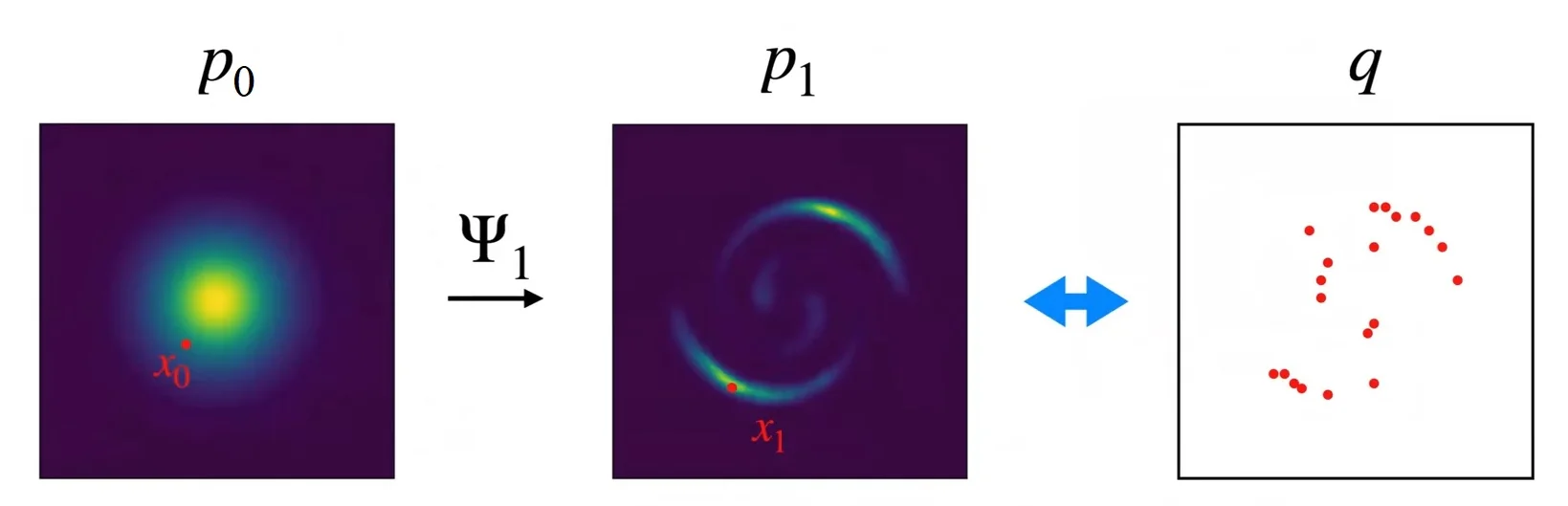
To compute or maximize the exact log-likelihood \( \log p_1(x_1) \), we must understand how the flow reshapes probability mass over time. This relationship is governed by the change-of-variables formula for differentiable bijections: \[ p_1(x_1) = p_0(x_0) \cdot \left | \det \left ( \frac {\partial \psi _1^{-1}}{\partial x_1} \right ) \right | = p_0(x_0) \cdot \left | \det \left ( \frac {\partial \psi _1}{\partial x_0} \right ) \right |^{-1}, \] where \( x_1 = \psi _1(x_0) \) and \( \frac {\partial \psi _1}{\partial x_0} \in \mathbb {R}^{d \times d} \) is the Jacobian matrix of \( \psi _1 \). The absolute value ensures volume is computed without assuming orientation.
This formula follows from standard results in multivariable calculus [553, Theorem 7.26]. In practice, models often optimize the log-density form: \[ \log p_1(x_1) = \log p_0(x_0) - \log \left | \det \left ( \frac {\partial \psi _1}{\partial x_0} \right ) \right |. \]
To understand the derivation, consider a measurable region \( A \subset \mathbb {R}^d \) and its image \( B = \psi _1(A) \). Since \( \psi _1 \) is invertible, the mass over \( A \) and \( B \) must match: \[ \int _A p_0(x_0) \, dx_0 = \int _B p_1(x_1) \, dx_1. \] Changing variables in the second integral yields: \[ \int _B p_1(x_1) \, dx_1 = \int _A p_1(\psi _1(x_0)) \cdot \left | \det J_{\psi _1}(x_0) \right | \, dx_0, \] where \( J_{\psi _1}(x_0) = \frac {\partial \psi _1}{\partial x_0} \). Equating both sides and canceling the integral over \( A \) gives: \[ p_0(x_0) = p_1(\psi _1(x_0)) \cdot \left | \det J_{\psi _1}(x_0) \right |, \] and solving for \( p_1 \) recovers the change-of-variables formula.
Intuitively, this result tracks how a small volume element transforms under \( \psi _1 \). The Jacobian determinant quantifies how the flow locally scales volume: if it expands space near \( x_0 \), the mass is diluted and the density decreases at \( x_1 \); if it contracts space, the density increases. In particular: \[ \left | \det \left ( \frac {\partial \psi _1}{\partial x_0} \right ) \right | > 1 \quad \Rightarrow \quad \mbox{volume expansion, lower density,} \] \[ \left | \det \left ( \frac {\partial \psi _1}{\partial x_0} \right ) \right | < 1 \quad \Rightarrow \quad \mbox{volume compression, higher density.} \] Hence, evaluating \( p_1(x_1) \) requires tracing the pre-image \( x_0 = \psi _1^{-1}(x_1) \) and correcting the base density \( p_0(x_0) \) by the inverse local volume scaling.
Discrete vs. Continuous Architectures. For standard discrete normalizing flows, computing the log-determinant of the Jacobian \( \log \left |\det \frac {\partial \psi }{\partial x}\right | \) scales cubically \( \mathcal {O}(d^3) \) in general. To make this tractable, architectures like RealNVP [130] and Glow [306] enforce strict structural constraints (e.g., triangular masks or \(1\times 1\) convolutions) to ensure the Jacobian is triangular or easily invertible.
Continuous Normalizing Flows (CNFs) [88] remove these architectural restrictions by modeling the transformation as an ODE driven by a velocity field \( v_t(x) \). By the Instantaneous Change of Variables theorem, the evolution of the log-density is governed not by a determinant, but by the divergence of the velocity field: \[ \frac {d}{dt} \log p_t(x_t) = - \nabla \cdot v_t(x_t). \] This formulation allows the use of arbitrary deep neural networks for \( v_t \). Furthermore, the divergence can be estimated efficiently (in \( \mathcal {O}(d) \)) using unbiased stochastic trace estimators (e.g., Hutchinson’s trick in FFJORD [191]), making CNFs scalable to high-dimensional data without imposing triangular structures.
The Role of the Continuity Equation To avoid computing high-dimensional Jacobian determinants, continuous-time flow models adopt a differential viewpoint. Instead of working directly with the global transformation \( \psi _1 \), we define a time-indexed velocity field \( v_t(x) \) that infinitesimally moves samples along trajectories \( x_t = \psi _t(x_0) \), starting from \( x_0 \sim p_0 \). The evolving distribution \( p_t \) induced by this flow changes continuously over time, and its dynamics are governed by the continuity equation: \[ \frac {\partial p_t(x)}{\partial t} + \nabla \cdot \left ( p_t(x) \, v_t(x) \right ) = 0. \] This equation formalizes the principle of local conservation of probability mass: the only way for density at a point \( x \) to change is via inflow or outflow of mass from its surrounding neighborhood.
To understand this equation precisely, let us examine the structure and roles of each term. We begin with the product \( p_t(x) \cdot v_t(x) \), often referred to as the probability flux.
Flux: Constructing \( p_t(x) v_t(x) \)
- \( p_t(x) \colon \mathbb {R}^d \to \mathbb {R} \) is a scalar field: it represents the probability density at each spatial point \( x \).
- \( v_t(x) \colon \mathbb {R}^d \to \mathbb {R}^d \) is a vector field: it assigns a velocity vector to each point in space and time.
The product \( p_t(x) v_t(x) \in \mathbb {R}^d \) is a vector-valued function defined componentwise: \[ (p_t v_t)(x) = \begin {bmatrix} p_t(x) v_{t,1}(x) \\ p_t(x) v_{t,2}(x) \\ \vdots \\ p_t(x) v_{t,d}(x) \end {bmatrix}. \] This object is called the probability flux vector field. It tells us, for each spatial coordinate direction \( i = 1, \dots , d \), the rate at which probability mass is moving through space in that direction. If the domain is \( \mathbb {R}^d \), the flux encodes how much mass is flowing through each coordinate axis — left/right, up/down, in/out — at every location and moment in time.
Intuitively, you can picture \( p_t(x) \) as the “density of fog” at point \( x \), and \( v_t(x) \) as the wind that moves the fog. Their product, \( p_t(x) v_t(x) \), describes how strongly the fog is being pushed in each direction. If the wind is fast but no fog is present, there’s no actual movement of mass. If fog is dense but wind is still, the same holds. Only when both density and velocity are present do we get mass transport.
Divergence: Understanding \( \nabla \cdot (p_t v_t) \) Despite involving the symbol \( \nabla \), the divergence operator is not a gradient. It maps a vector field \( \vec {F} : \mathbb {R}^d \to \mathbb {R}^d \) to a scalar field, and is defined as: \[ \nabla \cdot \vec {F}(x) = \sum _{i=1}^d \frac {\partial F_i(x)}{\partial x_i}. \] Applied to the flux vector \( p_t(x) v_t(x) \), we get: \[ \nabla \cdot (p_t v_t)(x) = \sum _{i=1}^d \frac {\partial }{\partial x_i} \left [ p_t(x) \cdot v_{t,i}(x) \right ]. \]
This scalar quantity captures the net rate of mass flow out of point \( x \) in all coordinate directions. For each dimension \( i \), it computes how much probability is flowing in or out through \( x_i \), and the sum tells us whether more mass is entering or exiting the region overall.
In this sense, divergence functions as a ”net-outflow meter”:
- If \( \nabla \cdot (p_t v_t)(x) > 0 \), more mass is exiting than entering — density decreases.
- If \( \nabla \cdot (p_t v_t)(x) < 0 \), more mass is arriving than leaving — density increases.
- If \( \nabla \cdot (p_t v_t)(x) = 0 \), inflow and outflow balance — density remains stable.
Unlike the gradient, which returns a vector pointing in the direction of steepest increase of a scalar field, the divergence is a scalar, that tells us whether the region is acting like a source (positive divergence) or a sink (negative divergence) of probability mass.
Putting the Continuity Equation in Plain English \[ \underbrace {\frac {\partial p_t(x)}{\partial t}}_{\mbox{\small temporal change at a fixed point}} \;+\; \underbrace {\nabla \cdot \left ( p_t(x) \, v_t(x) \right )}_{\mbox{\small net probability flowing \emph {out} of } x} \;=\; 0. \]
Think of \( p_t(x) \) as the density of a colored fog, and \( v_t(x) \) as a wind field that pushes the fog through space.
- Local accumulation: \( \displaystyle \frac {\partial p_t(x)}{\partial t} \) asks whether the fog at the fixed location \( x \) is getting thicker (\( > 0 \)) or thinner (\( < 0 \)) as time progresses. This is a temporal derivative: \( x \) is held fixed and we observe how the density changes with \( t \).
- Net inflow or outflow: \( \displaystyle \nabla \cdot \left ( p_t(x) v_t(x) \right ) \) measures the net rate at which probability mass exits an infinitesimal volume surrounding \( x \). Imagine placing a tiny box around \( x \); this term tells you how much mass escapes from the box minus how much enters it, per unit time.
The equation asserts that these two quantities exactly cancel: \[ \mbox{rate of local buildup} \;+\; \mbox{rate of escape} \;=\; 0. \]
No probability mass is created or destroyed—only transported. This is a local conservation law, the probabilistic analogue of classical principles like:
- conservation of mass in fluid dynamics,
- conservation of charge in electromagnetism.
For continuous-time generative models, the continuity equation provides a conceptual bridge between the microscopic law—how individual particles move under the velocity field \( v_t \)—and the macroscopic law—how the overall distribution \( p_t \) evolves over time.
Crucially, it allows us to reason about global changes in the distribution without explicitly computing expensive Jacobian determinants: the continuity equation already captures the effect of the full flow through a compact, pointwise identity.
Broader Implications for Continuous-Time Generative Models The continuity equation
\begin {equation} \tag {CE}\label {eq:chapter20_continuity_equation} \frac {\partial p_t(x)}{\partial t} + \nabla \cdot \left ( p_t(x)\,v_t(x) \right ) = 0. \end {equation}
is the probabilistic analogue of mass conservation in fluid dynamics. Any continuous-time generative model that defines trajectories via the ODE \[ \frac {d}{dt} x_t = v_t(x_t) \] must respect this equation to ensure that probability mass is preserved under the flow. Notable examples include Neural ODEs [88], FFJORD [191], and probability flow ODEs [605].
One of the most important consequences of this formulation is that it allows us to track the evolution of the log-density along a sample trajectory \( x_t \) without computing high-dimensional Jacobian determinants.
Step-by-step: How Log-Density Evolves Along the Flow
Let \( x_t \) be the solution to the ODE \( \dot {x}_t = v_t(x_t) \). To understand how the density \( p_t(x_t) \) changes along this trajectory, we apply the chain rule for total derivatives to the composition \( t \mapsto \log p_t(x_t) \): \[ \frac {d}{dt} \log p_t(x_t) = \underbrace {\frac {\partial }{\partial t} \log p_t(x)}_{\mbox{explicit time dependence}} + \underbrace {\nabla _x \log p_t(x) \cdot \frac {d x_t}{dt}}_{\mbox{motion along the path}} \bigg |_{x = x_t}. \] The first term captures how the log-density at a fixed spatial location changes over time. The second term accounts for how the log-density changes as the point \( x_t \) moves through space.
We now turn to the continuity equation: \[ \frac {\partial p_t(x)}{\partial t} + \nabla \cdot \left ( p_t(x)\,v_t(x) \right ) = 0. \] Assuming \( p_t(x) > 0 \), we divide through by \( p_t(x) \) to rewrite the equation in terms of \( \log p_t(x) \): \[ \frac {1}{p_t(x)} \frac {\partial p_t(x)}{\partial t} + \frac {1}{p_t(x)} \nabla \cdot \left ( p_t(x)\,v_t(x) \right ) = 0. \]
Using the identities: \[ \frac {\partial }{\partial t} \log p_t(x) = \frac {1}{p_t(x)} \frac {\partial p_t(x)}{\partial t}, \qquad \nabla \cdot \left ( p_t v_t \right ) = \nabla p_t \cdot v_t + p_t \nabla \cdot v_t, \] we substitute and rearrange: \[ \frac {\partial }{\partial t} \log p_t(x) = - \nabla \cdot v_t(x) - \nabla _x \log p_t(x) \cdot v_t(x). \]
Substituting this into the total derivative expression (and using \( \dot {x}_t = v_t(x_t) \)) gives: \[ \frac {d}{dt} \log p_t(x_t) = \left [ - \nabla \cdot v_t(x) - \nabla _x \log p_t(x) \cdot v_t(x) \right ] + \nabla _x \log p_t(x) \cdot v_t(x) \bigg |_{x = x_t}. \] The inner product terms cancel, leaving: \[ \frac {d}{dt} \log p_t(x_t) = - \nabla \cdot v_t(x_t). \]
This is the celebrated Liouville identity, which relates log-density dynamics to the divergence of the velocity field: \begin {equation} \boxed { \frac {d}{dt} \log p_t(x_t) = - \nabla \cdot v_t(x_t) } \end {equation}
Interpretation This equation reveals that the rate of change of log-density along the path of a particle is governed entirely by the local divergence of the velocity field at that point. If \( \nabla \cdot v_t > 0 \), the flow is expanding locally: volumes grow, so density must decrease. If \( \nabla \cdot v_t < 0 \), the flow is compressing: volumes shrink, so density increases. Hence, divergence acts as a local proxy for log-likelihood adjustment.
From here, we can integrate both sides over time to obtain an exact log-likelihood formula for a sample transformed through the flow: \[ \log p_1(x_1) = \log p_0(x_0) - \int _0^1 \nabla \cdot v_t(x_t) \, dt, \qquad x_1 = \psi _1(x_0). \] This shows that to evaluate \( \log p_1(x_1) \), we simply need to know the base log-density \( \log p_0(x_0) \) and integrate the divergence along the trajectory. No determinant or inverse map is needed.
This identity is the foundation of continuous normalizing flows (CNFs)—a class of generative models that define invertible mappings by continuously transforming a base distribution \( p_0 \) via a learned differential equation \( \frac {d}{dt} x_t = v_t(x_t) \).
CNFs generalize discrete normalizing flows by replacing sequences of invertible layers with a smooth velocity field, and they compute log-likelihoods exactly via the Liouville identity. This makes maximum-likelihood training in continuous-time models theoretically elegant and tractable, using numerical ODE solvers to trace sample trajectories and trace estimators (e.g., Hutchinson’s method) to approximate divergence.
Why Pure CNF–Likelihood Training Is Not Scalable? The Liouville identity provides an exact formula for the model likelihood in continuous-time generative models governed by an ODE \( \dot {x}_t = v_t(x_t) \): \[ \log p_1(x_1) = \log p_0(x_0) - \int _0^1 \nabla \cdot v_t(x_t) \, dt, \qquad x_1 = \psi _1(x_0). \] In theory, this makes continuous normalizing flows (CNFs) ideal candidates for maximum likelihood estimation. For a dataset of samples \( \{ x^{(i)}_{\mbox{data}} \} \), one could train the model by maximizing this likelihood with respect to the parameters of \( v_t \), using standard gradient-based optimization.
How training works in principle:
- 1.
- Reverse ODE step: For each data point \( x_1 = x^{(i)}_{\mbox{data}} \), solve the reverse-time ODE \[ \frac {d}{dt} x_t = -v_{1 - t}(x_t) \] backward from \( t = 1 \) to \( t = 0 \), yielding the latent code \( x_0 = \psi _1^{-1}(x_1) \).
- 2.
- Divergence accumulation: Along this trajectory, compute or estimate the integral \[ \int _0^1 \nabla \cdot v_t(x_t) \, dt \] using numerical quadrature.
- 3.
- Likelihood computation: Combine with the known base density \( p_0(x_0) \) to evaluate \[ \log p_1(x_1) = \log p_0(x_0) - \int _0^1 \nabla \cdot v_t(x_t) \, dt. \]
- 4.
- Optimization: Backpropagate through all of the above to update the parameters of \( v_t \) to maximize the total log-likelihood over the dataset.
While theoretically elegant, this “textbook” maximum likelihood strategy faces major barriers in practice—especially when scaling to high-dimensional data such as natural images.
Where the computational cost comes from:
- 1.
- Trajectory integration. Every forward (or reverse) pass requires numerically solving the ODE \( \dot {x}_t = v_t(x_t) \) over \( t \in [0,1] \). Adaptive solvers like Runge–Kutta may need 30–200 function evaluations, depending on the stiffness and complexity of \( v_t \).
- 2.
- Divergence computation. The divergence \( \nabla \cdot v_t(x_t) \) is the trace of the Jacobian \( \nabla _x v_t \in \mathbb {R}^{d \times d} \). Estimating this exactly costs \( \mathcal {O}(d^2) \), or up to \( \mathcal {O}(d^3) \) with autodiff. Hutchinson’s stochastic trace estimator [191] reduces the cost to \( \mathcal {O}(d) \) but introduces variance that must be averaged out over multiple random vectors.
- 3.
- Backpropagation. Training requires gradients of the loss with respect to the parameters of \( v_t \), which depends on the full trajectory. This necessitates differentiating through the ODE solver. Adjoint sensitivity methods [88] reduce memory use, but can be numerically unstable and roughly double the runtime.
- 4.
- Slow sampling. Unlike discrete normalizing flows, CNFs require solving the forward ODE \( \dot {x}_t = v_t(x_t) \) even at inference time for each latent \( x_0 \sim p_0 \). Sampling is thus orders of magnitude slower than a feedforward network.
Additionally: score-based dependencies. Some continuous-time models incorporate score terms \( \nabla _x \log p_t(x) \), either to guide learning or to define velocity fields indirectly. These score functions are difficult to estimate robustly in high dimensions and often lead to unstable gradients or high variance during training.
Modern practice. Because of these practical limitations, state-of-the-art CNF-based models often avoid direct maximum likelihood training altogether:
- FFJORD [191] uses Hutchinson’s trick to estimate the divergence efficiently, but is still limited to low-resolution datasets like CIFAR-10 (\( 32 \times 32 \)).
- Probability flow ODEs [605] sidestep likelihood computation during training by learning the score function \( \nabla _x \log p_t(x) \) using denoising score-matching losses. The ODE is only used at test time for generation.
- Hybrid methods perform training with diffusion-style objectives and sample deterministically with few ODE steps (as in DDIM or ODE-based sampling), achieving good sample quality at lower cost.
Flow Matching: A New Approach While the Liouville identity enables exact likelihood estimation in continuous normalizing flows (CNFs), its practical use is limited by the computational cost of integrating trajectories, estimating divergence, and backpropagating through ODE solvers—especially in high-dimensional settings like natural images.
This leads to a natural question:
Can we avoid computing densities or their derivatives—and directly learn how to transport mass from \( p_0 \) to \( p_1 \)?
Flow Matching [373] answers this affirmatively. It reframes generative modeling as supervised learning over velocity fields—sidestepping the need for log-densities, Jacobians, or variational objectives.
Given a chosen coupling (joint distribution) \( \pi (x_0,x_1) \) between the base \(p_0\) and the data distribution \(q\), we can sample endpoint pairs \( (x_0,x_1)\sim \pi \) and define an explicit interpolant \( x_t = \phi _t(x_0,x_1) \) for \( t\in [0,1] \). A common and especially simple choice is the linear interpolant \[ x_t = (1-t)x_0 + t x_1, \qquad \Rightarrow \qquad \frac {d}{dt}x_t = x_1 - x_0, \] which traces straight lines in sample space between paired endpoints.
Flow Matching [373] trains a neural velocity field \(v_\theta (x,t)\) by supervised regression to match the (conditional) time-derivative of the chosen interpolant. Informally, the learning target is the instantaneous transport direction that would move samples along the prescribed path; no log-densities, Jacobians, ELBOs, or score estimates are required during training. Once trained, generation draws \(x_0\sim p_0\) and integrates the learned ODE \[ \frac {d}{dt}x_t = v_\theta (x_t,t), \qquad x_0\sim p_0, \] to obtain \(x_1\).
This is conceptually different from diffusion “\(v\)-prediction” (or “\(v\)-space”): in diffusion, \(v\) is a reparameterization of a denoising objective tied to a Gaussian noising process; in flow matching, the network is trained to approximate an actual transport velocity for a user-chosen probability path (often constructed to be geometrically simple, e.g., straight in sample space).
Enrichment 20.10.2: Development of the Flow Matching Objective
From Density Path to Vector Field The Flow Matching objective is rooted in the relationship between a time-evolving probability distribution \( \{p_t(x)\}_{t \in [0,1]} \) and the velocity field \( u_t(x) \) that transports mass along this path. This relationship is formalized by the continuity equation: \[ \frac {\partial p_t(x)}{\partial t} + \nabla \cdot \left ( p_t(x) u_t(x) \right ) = 0. \] This PDE expresses local conservation of probability mass: the change in density at a point is exactly offset by the net flow of mass in or out.
Crucially, the continuity equation can also be read in reverse: if we prescribe a sufficiently regular density path \( \{p_t\}_{t\in [0,1]} \), then any velocity field \(u_t\) that generates this path must satisfy the inverse constraint \[ \nabla \cdot \bigl (p_t(x)\,u_t(x)\bigr ) \;=\; -\,\partial _t p_t(x). \] It is often convenient to phrase this in terms of the probability flux \(j_t(x) := p_t(x)\,u_t(x)\), in which case the constraint becomes the Poisson-type divergence equation \[ \nabla \cdot j_t(x) \;=\; -\,\partial _t p_t(x). \]
Importantly, this inverse problem does not determine \(u_t\) uniquely: if \(w_t\) satisfies \( \nabla \cdot \!\bigl (p_t w_t\bigr )=0 \), then \(u_t+w_t\) induces the same density evolution. Equivalently, a density path typically admits infinitely many generating vector fields, differing by divergence-free components in the appropriate weighted sense.
When one wants a canonical choice, a common restriction is to consider potential (gradient) flows \(u_t=\nabla \phi _t\), which yields the elliptic PDE \[ \nabla \cdot \bigl (p_t(x)\,\nabla \phi _t(x)\bigr ) \;=\; -\,\partial _t p_t(x). \] However, Flow Matching will not attempt to solve such global PDEs. Instead, it constructs conditional paths and conditional vector fields in closed form, and then uses them to obtain a tractable supervised objective.
This insight is the foundation of Flow Matching: specifying a density path \(\{p_t\}\) constrains the probability flux \(j_t=p_t u_t\) through the continuity equation, and it determines a particular generating field \(u_t\) only after we fix a convention (a “gauge”) or explicitly construct the flow map. Flow Matching avoids solving the global inverse PDE by designing conditional paths for which the associated velocity field is available in closed form, enabling supervised regression of \(v_\theta \).
The Naive Flow Matching Objective This motivates the general Flow Matching training loss:
\begin {equation} \mathcal {L}_{\mathrm {FM}}(\theta ) = \mathbb {E}_{t \sim \mathcal {U}(0,1),\, x \sim p_t} \left [ \|v_\theta (t, x) - u_t(x)\|_2^2 \right ]. \label {eq:chapter20_fm_naive} \end {equation}
where:
- \( v_\theta (t,x) \) is a learnable velocity field (e.g., a neural network with parameters \( \theta \)),
- \( u_t(x) \) is the ground-truth velocity field that satisfies the continuity equation for the path \( \{p_t\} \),
- \( x \sim p_t \) denotes that samples are drawn from the intermediate distribution at time \( t \),
- \( t \sim \mathcal {U}[0,1] \) is sampled uniformly across time.
Intuitively, this objective trains the CNF vector field \( v_\theta \) to reproduce the flow that transports the mass of \( p_0 \) to \( p_1 \) via the path \( \{p_t\} \). If the regression error reaches zero, then integrating \( v_\theta \) over time from \( t=0 \) to \( t=1 \) recovers the exact map \( \psi _t \) that generates the full path, including the final distribution \( p_1(x) \approx q(x) \).
Why the Naive Objective Is Intractable While the Flow Matching loss provides a clean supervised objective, applying it naively in practice proves infeasible. The loss \[ \mathcal {L}_{\mathrm {FM}}(\theta ) = \mathbb {E}_{t \sim \mathcal {U}[0,1],\, x \sim p_t} \left [ \|v_\theta (t, x) - u_t(x)\|^2 \right ] \] assumes access to both the intermediate density \( p_t \) and the corresponding vector field \( u_t \) at every point in space and time. But in real-world generative modeling settings, neither of these quantities is known in closed form.
First, the interpolation path \( \{p_t\} \) is fundamentally underdetermined: there are infinitely many ways to transition from \( p_0 \) to \( p_1 \), each leading to a different transport behavior. Whether we interpolate linearly in sample space, follow heat diffusion, or traverse a Wasserstein geodesic, each path implies a different evolution of probability mass—and a different target field \( u_t \).
Even if we fix a reasonable interpolation scheme, we still face two practical barriers:
- We typically cannot sample from \( p_t(x) \) at arbitrary times.
- We cannot compute \( u_t(x) \), since it involves inverting the continuity equation—a PDE that depends on time derivatives and spatial gradients of \( p_t \).
In short, the general form of the FM loss assumes a full global picture of how mass moves from \( p_0 \) to \( p_1 \)—but in practice, we only have endpoint samples: \( x_0 \sim p_0 \) (a known prior) and \( x_1 \sim p_1 \approx q(x) \) (empirical data). We know nothing about the intermediate distributions \( p_t \), nor their generating vector fields.
A Local Solution via Conditional Paths To sidestep the intractability of a global path \(\{p_t\}\), Flow Matching constructs a family of analytically tractable conditional paths \(\{p_t(\cdot \mid x_1)\}_{t\in [0,1]}\) indexed by an endpoint sample \(x_1\sim q\). The key move is to define each conditional path as the pushforward of the base distribution \(p_0\) through an explicit time-dependent map \(\psi _t(\cdot \mid x_1)\): \[ x_0 \sim p_0, \qquad x_t := \psi _t(x_0 \mid x_1), \qquad p_t(\cdot \mid x_1) := \bigl (\psi _t(\cdot \mid x_1)\bigr )_{\#} p_0. \] The conditional velocity field is then defined by construction as the time derivative of the flow map along trajectories: \[ u_t(x\mid x_1) := \left .\frac {\partial }{\partial t}\psi _t(x_0\mid x_1)\right |_{x_0=\psi _t^{-1}(x\mid x_1)}. \]
Affine conditional maps (diffusion- and OT-style paths). A particularly convenient choice is an affine map \[ \psi _t(x_0\mid x_1)=\sigma _t x_0 + \mu _t(x_1), \] with scalar \(\sigma _t>0\) and a mean function \(\mu _t(\cdot )\). In this case, \(\psi _t^{-1}(x\mid x_1)=(x-\mu _t(x_1))/\sigma _t\), and the induced conditional velocity has a closed form: \[ u_t(x\mid x_1) = \frac {\dot {\sigma }_t}{\sigma _t}\bigl (x-\mu _t(x_1)\bigr ) + \dot {\mu }_t(x_1), \] where dots denote time derivatives.
OT straight-line special case (constant-velocity parameterization). Choosing \(\sigma _t=1-t\) and \(\mu _t(x_1)=t x_1\) yields the familiar linear interpolation \[ x_t=\psi _t(x_0\mid x_1)=(1-t)x_0+t x_1, \] so each sample follows a straight line from \(x_0\sim p_0\) toward \(x_1\sim q\). Crucially, if we define the conditional velocity field by differentiating the flow map with respect to time while holding the sampled start point \(x_0\) fixed, then the velocity along the realized trajectory is \[ u_t(x_t \mid x_0,x_1) = \frac {d}{dt}\bigl ((1-t)x_0+t x_1\bigr ) = x_1-x_0, \] which is constant in \(t\) and numerically stable.
One can also rewrite this same target purely in terms of \((t,x_t,x_1)\) as \[ u_t(x_t\mid x_1)=\frac {x_1-x_t}{1-t}, \] since \(x_0=(x_t-t x_1)/(1-t)\). This form is algebraically equivalent but is typically ill-conditioned as \(t\to 1\) due to the explicit division by \((1-t)\). In practice (and in modern “constant-velocity” training), we therefore keep \(x_0\) as an auxiliary sampled variable and regress directly to \(x_1-x_0\).
Equivalently, this construction can be viewed as sampling a pair \((x_0,x_1)\) from a coupling \(\pi \) with marginals \(p_0\) and \(q\): the default choice is the independent coupling \(p_0\times q\), while alternative couplings (e.g., minibatch OT) change which straight segments are emphasized.
From Conditional Paths to a Marginal Path Given a coupling \(\pi (x_0,x_1)\) between \(p_0\) and \(q\), and an explicit pair-conditioned map \(x_t=\psi _t(x_0,x_1)\), the induced marginal at time \(t\) is simply the pushforward of \(\pi \) through \(\psi _t\): \[ p_t = (\psi _t)_{\#}\pi . \] Equivalently, in density form, \[ p_t(x) = \iint \delta \!\bigl (x-\psi _t(x_0,x_1)\bigr )\,\pi (x_0,x_1)\,dx_0\,dx_1. \]
For the independent coupling \(\pi =p_0\times q\), this reduces to sampling \(x_0\sim p_0\), \(x_1\sim q\), and pushing the pair through \(\psi _t\). If the endpoint condition satisfies \(\psi _{t=1}(x_0,x_1)=x_1\) \(\pi \)-almost surely (e.g., the OT/rectified linear map with \(\sigma (1)=0\)), then \(p_{t=1}=q\).
Conditional Flow Matching (CFM): A Tractable Objective The CFM training objective is a supervised regression problem built from samples of the conditional path.
Operationally, we sample a time and an endpoint, and we also sample the auxiliary start point used by the pushforward construction: \[ t \sim \mathcal {U}(0,1), \quad (x_0,x_1)\sim \pi \ \ (\mbox{e.g., }\pi =p_0\times q \mbox{ or minibatch OT}) , \quad x_t := \psi _t(x_0\mid x_1). \] For OT-style linear interpolation, \(x_t=(1-t)x_0+t x_1\), and the analytic target is the constant velocity \(u_t(x_t\mid x_0,x_1)=x_1-x_0\). We then fit \(v_\theta \) by squared error:
\begin {equation} \boxed { \mathcal {L}_{\mathrm {CFM}}(\theta ) = \mathbb {E}_{t \sim \mathcal {U}(0,1),\, (x_0,x_1)\sim \pi } \left [ \left \| v_\theta (t, x_t) - (x_1-x_0) \right \|_2^2 \right ]} \label {eq:chapter20_cfm} \end {equation}
What is (and is not) conditioned on. In the unconditional generative setting, \(v_\theta (t,x)\) does not take \((x_0,x_1)\) as input. The pair \((x_0,x_1)\) is used only to (i) construct a training sample \(x_t\) on the conditional path and (ii) compute the analytic regression target (e.g., \(x_1-x_0\) for OT-style paths). At optimum, this recovers the marginal field as a conditional expectation over the coupling, consistent with the Flow Matching theory.
In this section we do not yet commit to a specific form of \( p_t(x \mid x_1) \), but crucially, the framework allows any analytic choice—so long as it satisfies appropriate boundary conditions and yields a velocity field computable in closed form. In the next section, we explore such constructions explicitly.
Why is this valid? Flow Matching shows that the conditional regression loss used in CFM is an unbiased surrogate for the intractable marginal FM objective: under mild regularity assumptions, both objectives induce the same parameter gradients when the conditional path is constructed as in CFM. Equivalently, the optimal unconditional field corresponds to the appropriate conditional expectation of the analytic conditional velocity targets, so integrating \(\dot {x}_t=v_\theta (t,x_t)\) transports \(p_0\) along the intended marginal path. See Theorem 2 and Appendix A of [373].
The proof relies on rewriting both losses using bilinearity of the squared norm, and applying Fubini’s Theorem to swap the order of integration over \( x \) and \( x_1 \). The core insight is that the marginal field \( u_t(x) \) is itself an average over the conditional fields \( u_t(x \mid x_1) \), making CFM an unbiased surrogate for the original objective. For a detailed derivation, see Appendix A of [373].
Why This Is Powerful The Conditional Flow Matching objective unlocks a practical and scalable method for training continuous-time generative models. It removes the need to estimate intermediate marginals or evaluate global velocity fields—obstacles that make the original FM loss intractable in high dimensions.
Moreover, this framework is highly flexible: so long as we define a valid conditional path \( p_t(x \mid x_1) \) with known boundary conditions and an analytic velocity field \( u_t(x \mid x_1) \), we can train a model using only endpoint samples \( (x_0, x_1) \sim p_0 \times q \). This enables a wide variety of conditional designs, each inducing distinct training behavior and inductive biases.
In the next part, we introduce several tractable and theoretically grounded choices for the conditional trajectory \( p_t(x \mid x_1) \) and its corresponding vector field \( u_t(x \mid x_1) \), including Gaussian interpolants and optimal transport-inspired paths.
Enrichment 20.10.3: Conditional Flow Matching
Motivation (Why condition on pairs?) The goal of Flow Matching is to learn a global velocity field \(v_\theta (t,x)\) whose ODE transports a simple base distribution \(p_0\) (e.g., Gaussian noise) into the data distribution \(q\). Directly specifying the marginal path \(\{p_t\}_{t\in [0,1]}\) and its generating field is typically intractable. Instead, modern Conditional Flow Matching (CFM) defines the global path as a superposition of conditional trajectories indexed by pairs \((x_0,x_1)\), with \(x_0\sim p_0\), \(x_1\sim q\), and \((x_0,x_1)\sim \pi \) for some coupling \(\pi \) (the default is independent \(\pi =p_0\times q\); stronger choices include minibatch OT couplings).
Conditioning on \((x_0,x_1)\) is not just a modeling convenience: it lets us obtain a stable, closed-form supervision signal as a plain time derivative of an explicitly designed interpolation. This avoids the numerically stiff “state-space” expressions that arise when one conditions only on an endpoint \(x_1\) and rewrites velocities using ratios like \(\dot {\sigma }(t)/\sigma (t)\) as \(\sigma (t)\to 0\).
Choosing Conditional Paths – Diffusion vs. OT
A unifying template: affine conditional flows on pairs The most widely used family in practice is the class of affine conditional flow maps \begin {equation} x_t \;=\; \psi _t(x_0,x_1) \;:=\; \sigma (t)\,x_0 \;+\; \alpha (t)\,x_1, \qquad t\in [0,1], \label {eq:chapter20_affine_pair_path} \end {equation} with boundary conditions \[ \sigma (0)=1,\ \alpha (0)=0 \qquad \mbox{and}\qquad \sigma (1)=0,\ \alpha (1)=1, \] so that \(x_{t=0}=x_0\) and \(x_{t=1}=x_1\). (In practice, one may use \(\sigma (1)=\sigma _{\min }>0\) to avoid endpoint degeneracy; see below.)
The stable regression target: the trajectory derivative For a fixed pair \((x_0,x_1)\), the conditional velocity along the realized trajectory \(x_t=\psi _t(x_0,x_1)\) is by construction the time derivative: \begin {equation} u_t(x_t \mid x_0,x_1) \;:=\; \frac {d}{dt}\psi _t(x_0,x_1) \;=\; \dot {\sigma }(t)\,x_0 \;+\; \dot {\alpha }(t)\,x_1, \label {eq:chapter20_affine_pair_velocity} \end {equation} where dots denote derivatives with respect to \(t\). This is the supervision signal used in affine pair-based CFM: it is computed directly from \((x_0,x_1,t)\) and remains numerically well-behaved even when \(\sigma (t)\to 0\) near \(t\to 1\).
Remark (where the apparent singularity comes from). If one eliminates \(x_0\) using \(x_t=\sigma (t)x_0+\alpha (t)x_1\) (so \(x_0=(x_t-\alpha (t)x_1)/\sigma (t)\)), then (20.99) can be written as an endpoint-conditioned field \begin {equation} u_t(x \mid x_1) \;=\; \frac {\dot {\sigma }(t)}{\sigma (t)}\bigl (x-\alpha (t)x_1\bigr ) \;+\; \dot {\alpha }(t)\,x_1. \label {eq:chapter20_endpoint_conditioned_field} \end {equation} This is mathematically correct for \(t<1\), but it exposes the classical stiffness mechanism: if \(\sigma (t)\to 0\), then \(\dot {\sigma }(t)/\sigma (t)\) typically diverges. The pair-based target (20.99) avoids this division entirely.
Two prominent choices: diffusion-inspired vs. OT/rectified Within the affine template (20.98), the difference between “diffusion” and “OT” paths is entirely the choice of schedules \(\alpha (t)\) and \(\sigma (t)\):
- Diffusion-inspired (curved) paths: \((\alpha (t),\sigma (t))\) are chosen from a diffusion noise schedule (often VP-style), yielding nonlinear coefficient trajectories and time-varying velocities.
- OT/rectified (straight) paths: \((\alpha (t),\sigma (t))\) are chosen to make sample trajectories as straight as possible, yielding the simplest constant-velocity supervision in the canonical case.
Diffusion-inspired affine paths (VP geometry)
Diffusion models can be viewed as specifying a signal-to-noise schedule; in the affine pair setting, this corresponds to selecting an increasing “signal” coefficient \(\alpha (t)\) and decreasing “noise” coefficient \(\sigma (t)\).
Variance-preserving (VP) family as an affine pair path A common diffusion-inspired choice enforces \[ \alpha (t)^2 + \sigma (t)^2 = 1, \] which can be interpreted geometrically as moving \((\alpha (t),\sigma (t))\) along the unit circle. A canonical example is the cosine schedule \begin {equation} \alpha (t)=\sin \!\left (\frac {\pi t}{2}\right ), \qquad \sigma (t)=\cos \!\left (\frac {\pi t}{2}\right ). \label {eq:chapter20_vp_cosine_schedule} \end {equation} This yields \[ x_t = \cos \!\left (\frac {\pi t}{2}\right )x_0 + \sin \!\left (\frac {\pi t}{2}\right )x_1, \] and the (stable) CFM target is the derivative \[ u_t(x_t\mid x_0,x_1) = -\frac {\pi }{2}\sin \!\left (\frac {\pi t}{2}\right )x_0 + \frac {\pi }{2}\cos \!\left (\frac {\pi t}{2}\right )x_1. \]
Why this is “curved”. Even though \(x_t\) lies in the span of \(\{x_0,x_1\}\), the coefficients are non-affine in \(t\), so the trajectory is generally not a straight-line segment between \(x_0\) and \(x_1\). Equivalently, the direction of the velocity varies with time because the relative weights on \(x_0\) and \(x_1\) vary nonlinearly.
Limitations of diffusion-inspired paths (in the CFM context) Diffusion-inspired schedules are expressive and well-studied, but they can be less attractive as a default in modern CFM implementations:
- Time-varying velocity: for a fixed pair \((x_0,x_1)\), the target depends on \(t\), increasing regression complexity.
- Higher curvature trajectories: nonlinear coefficient schedules often increase ODE solver effort at inference.
- Endpoint stiffness in endpoint-conditioned form: rewriting as \(u_t(x\mid x_1)\) often introduces factors like \(\dot {\sigma }(t)/\sigma (t)\) as \(\sigma (t)\to 0\), producing large magnitudes near \(t\to 1\).
Optimal Transport / rectified paths (straight lines, constant velocity)
OT intuition (distribution-space straightness) For quadratic cost, OT defines the Wasserstein-2 distance \[ W_2^2(p_0,p_1)=\inf _{\gamma \in \Gamma (p_0,p_1)}\int \|x-y\|^2\,d\gamma (x,y), \] and McCann’s displacement interpolation yields a geodesic in Wasserstein space via straight-line particle trajectories along an optimal coupling [432]. In the CFM setting, we emulate this “straightening” principle at the level of pair-conditioned trajectories.
The canonical OT/rectified schedule The simplest (and most important) choice is the linear schedule \begin {equation} \alpha (t)=t, \qquad \sigma (t)=1-t, \label {eq:chapter20_ot_schedule} \end {equation} giving the straight-line interpolation \[ x_t = (1-t)x_0 + t x_1. \] Differentiating yields the constant-velocity target \begin {equation} u_t(x_t\mid x_0,x_1) = \frac {d}{dt}\bigl ((1-t)x_0+t x_1\bigr ) = x_1 - x_0, \label {eq:chapter20_ot_constant_velocity} \end {equation} which is independent of \(t\) and does not explode as \(t\to 1\). This is the canonical supervision signal emphasized by rectified/OT-style flow matching: learn an ODE that follows straight paths between paired samples as much as possible.
Practical endpoint regularization via \(\sigma _{\min }\) Some implementations replace \(\sigma (1)=0\) by a small \(\sigma _{\min }>0\) to avoid degeneracy at \(t=1\), using \[ \sigma (t)=1-(1-\sigma _{\min })t, \qquad \alpha (t)=t, \] so that \(x_{t=1}=x_1+\sigma _{\min }x_0\) is a slightly “blurred” endpoint. The derivative target remains time-independent: \[ u_t(x_t\mid x_0,x_1) = \dot {\sigma }(t)x_0+\dot {\alpha }(t)x_1 = -(1-\sigma _{\min })x_0 + x_1. \] One can anneal \(\sigma _{\min }\) or integrate only to \(t=1-\varepsilon \) when an exactly sharp endpoint is desired.
Vector field geometry: diffusion vs. OT/rectified The key distinction is simplest at the level of pair-conditioned supervision:
- Diffusion-inspired: \(u_t(x_t\mid x_0,x_1)=\dot {\sigma }(t)x_0+\dot {\alpha }(t)x_1\) varies with \(t\) for most schedules, inducing higher curvature trajectories.
- OT/rectified: \(u_t(x_t\mid x_0,x_1)=x_1-x_0\) (or its \(\sigma _{\min }\)-regularized variant) is constant in time, yielding the simplest regression target and typically the least stiff dynamics.
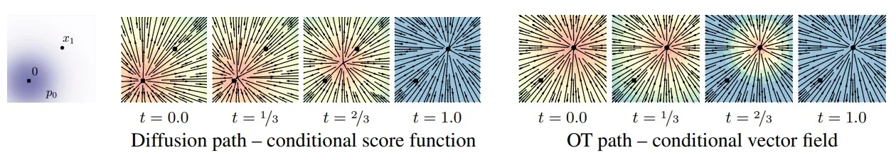
Why OT/rectified paths often provide a superior learning signal
- 1.
- Constant-velocity supervision (simplest regression problem). For OT/rectified interpolation, the model regresses a time-independent target vector \(x_1-x_0\) (per pair), reducing learning complexity.
- 2.
- Reduced endpoint stiffness. Endpoint-conditioned diffusion fields often contain factors like \(\dot {\sigma }(t)/\sigma (t)\) as \(\sigma (t)\to 0\), producing large magnitudes near \(t\to 1\). OT/rectified supervision avoids this: the target remains finite and constant in time.
- 3.
- Straighter trajectories (easier numerical integration). Straight-line paths minimize curvature at the trajectory level, often enabling accurate sampling with substantially fewer ODE solver steps.
- 4.
- Coupling improvements via minibatch OT / rectification. The coupling \(\pi (x_0,x_1)\) controls which straight segments are emphasized. Pairing “more compatible” \(x_0\) and \(x_1\) (e.g., via minibatch OT) reduces target variance and can further straighten trajectories.
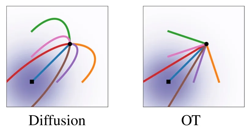
Conditional Flow Matching loss (pair-based, affine form) Let \(\pi (x_0,x_1)\) be any coupling of \(p_0\) and \(q\). The affine pair-based CFM objective is the regression of \(v_\theta \) to the conditional velocity target: \begin {equation} \boxed { \mathcal {L}_{\mathrm {CFM}}(\theta ) = \mathbb {E}_{(x_0,x_1)\sim \pi ,\ t\sim \mathcal {U}[0,1]} \left [ \left \| v_\theta \!\bigl (t, x_t\bigr ) - \bigl (\dot {\sigma }(t)x_0+\dot {\alpha }(t)x_1\bigr ) \right \|_2^2 \right ], } \label {eq:chapter20_affine_pair_cfm_loss} \end {equation} where \(x_t=\sigma (t)x_0+\alpha (t)x_1\). Crucially, in the unconditional generative setting the network does not take \(x_1\) as an input: \(x_1\) is used only to construct \((x_t,u_t)\) during training. (In conditional generation, \(v_\theta \) typically takes additional conditioning \(c\) such as text embeddings; this does not change the derivation).
From theory to practice: stable training loop (diffusion vs. OT)
- 1.
- Sample endpoints: Draw data \(x_1^{(i)} \sim q\) and noise \(x_0^{(i)} \sim \mathcal {N}(0,I)\) for \(i=1,\dots ,B\).
- 2.
- Couple (optional): To straighten paths, pair \(x_0\) and \(x_1\) by solving a discrete OT problem (linear sum assignment) on the batch distances, yielding a permutation \(\pi \). Replace \(x_0^{(i)} \leftarrow x_0^{(\pi (i))}\).
- 3.
- Sample times: Draw \(t^{(i)} \sim \mathcal {U}[0,1]\).
- 4.
- Compute target: Calculate the interpolated state \(x_t\) and its time derivative \(u_t\): \[ x_t^{(i)} = \sigma (t^{(i)})\,x_0^{(i)} + \alpha (t^{(i)})\,x_1^{(i)}, \qquad u_t^{(i)} = \dot {\sigma }(t^{(i)})\,x_0^{(i)} + \dot {\alpha }(t^{(i)})\,x_1^{(i)}. \]
- 5.
- Update: Gradient descent on the Mean Squared Error: \[ \mathcal {L} = \frac {1}{B}\sum _{i=1}^B \left \| v_\theta (t^{(i)}, x_t^{(i)}) - u_t^{(i)} \right \|_2^2. \]
Common Path Schedules:
- Linear / CondOT (The ”Rectified” Choice): Set \(\alpha (t)=t, \sigma (t)=1-t\). The derivatives are constant \(\dot {\alpha }=1, \dot {\sigma }=-1\). \[ \implies u_t = x_1 - x_0 \quad (\mbox{Constant Velocity}). \]
- Diffusion-Inspired (Variance Preserving): Set \(\alpha (t)=\sin (\frac {\pi t}{2}), \sigma (t)=\cos (\frac {\pi t}{2})\). \[ \implies u_t \mbox{ is time-varying and rotational (curved path).} \]
Inference: Solving the ODE Once trained, the network \(v_\theta (t,x)\) acts as the velocity field of an ODE. We generate samples by integrating from noise (\(t=0\)) to data (\(t=1\)). Because Linear/OT paths are nearly straight, we can often use simple solvers with very few steps (NFE).
- 1.
- Initialize \(x \sim \mathcal {N}(0,I)\), set step size \(dt = 1/N\).
- 2.
- For \(k=0\) to \(N-1\):
- Current time \(t_k = k/N\).
- Update position: \(x \leftarrow x + v_\theta (t_k, x) \cdot dt\).
- 3.
- Return \(x\) (approximate sample from \(q\)).
Note: If paths are slightly curved, the Midpoint (Heun) method is a common alternative that doubles accuracy for \(2\times \) cost.
- Time Embeddings: Do not feed the raw scalar \(t\) directly into the network. Map it through high-frequency sinusoidal features (Fourier embeddings) or a learned MLP to ensure the network is sensitive to small time changes.
- Broadcasting: Ensure \(t\) and its embeddings are correctly broadcast to match the spatial dimensions of \(x\) (e.g., \([B, C, H, W]\)).
- Coupling Benefits: Using Minibatch OT (step 2 above) significantly reduces the variance of the target \(x_1 - x_0\), making the regression task easier and the final flows straighter.
Takeaway Affine CFM demystifies continuous generative models by separating geometry (the path coefficients \(\alpha , \sigma \)) from learning (regressing the velocity). The simple Linear Schedule (\(u_t = x_1 - x_0\)) is the modern default because it yields the simplest training target and the most efficient inference trajectories.
Enrichment 20.10.4: Implementation, Experiments, and Extensions
Implementation Details Practitioners interested in applying Conditional Flow Matching (CFM) to their own datasets can refer to the following codebases:
- Official Flow Matching:
https://github.com/facebookresearch/flow_matching
A clean PyTorch library for Flow Matching, including both continuous and discrete formulations, with runnable examples and notebooks. - Conditional Flow Matching for High-Dimensional Data
(TorchCFM):
https://github.com/atong01/conditional-flow-matching
A practical CFM implementation for image datasets (e.g., CIFAR-10, CelebA) with U-Net backbones, training scripts, and sampling pipelines.
At a high level, both codebases implement the same supervised regression template. One samples endpoint pairs \(x_0 \sim \mathcal {N}(0,I)\) and \(x_1 \sim q(x)\), draws \(t \sim \mathrm {Unif}[0,1]\), constructs an intermediate state \(x_t = \psi _t(x_0 \mid x_1)\), and minimizes \[ \mathcal {L}_{\mathrm {CFM}}(\theta ) = \mathbb {E}\left [ \left \| v_\theta (t, x_t) - \frac {d}{dt}\psi _t(x_0, x_1) \right \|_2^2 \right ]. \]
In the unconditional setting, \(v_\theta \) takes only \((t,x)\) as input; in conditional generation, one augments the input with conditioning \(c\) (e.g., text), without changing the analytic target construction.
This yields scalable training without explicitly evaluating score functions \(\nabla _x \log p_t(x)\) or marginal likelihood terms.
Empirical Results: OT vs. Diffusion The choice of conditional probability path has a visible effect on both optimization and sampling. The Flow Matching paper [373] shows that OT-based conditional vector fields tend to induce straighter and more spatially coherent trajectories than diffusion-based paths, leading to earlier emergence of global structure and more efficient integration.

Quantitative Benchmarks Table 20.6 compares Flow Matching against diffusion- and score-based baselines on standard likelihood and sample-quality metrics. OT-FM consistently improves negative log-likelihood (NLL) and Fréchet Inception Distance (FID) while also reducing the number of function evaluations (NFE), reflecting cheaper ODE-based sampling at comparable quality.
| Model | CIFAR-10 | ImageNet \(32\times 32\) | ImageNet \(64\times 64\) |
||||||
|---|---|---|---|---|---|---|---|---|---|
| NLL \(\downarrow \) | FID \(\downarrow \) | NFE \(\downarrow \) | NLL \(\downarrow \) | FID \(\downarrow \) | NFE \(\downarrow \) | NLL \(\downarrow \) | FID \(\downarrow \) | NFE \(\downarrow \) | |
| DDPM [232] | 3.12 | 7.48 | 274 | 3.54 | 6.99 | 262 | 3.32 | 17.36 | 264 |
| Score Matching | 3.16 | 19.94 | 242 | 3.56 | 5.68 | 178 | 3.40 | 19.74 | 441 |
| ScoreFlow [605] | 3.09 | 20.78 | 428 | 3.55 | 14.14 | 195 | 3.36 | 24.95 | 601 |
| FM (Diffusion path) | 3.10 | 8.06 | 183 | 3.54 | 6.37 | 193 | 3.33 | 16.88 | 187 |
| FM (OT path) | 2.99 | 6.35 | 142 | 3.53 | 5.02 | 122 | 3.31 | 14.45 | 138 |
Additional Comparisons (High-Resolution ImageNet) For higher-resolution settings (e.g., ImageNet \(128\times 128\)), the same work reports competitive sample quality relative to several GAN-based baselines, while also providing a tractable likelihood objective.
Flow Matching (FM) sits at the intersection of three lines of work:
- Score-Based Generative Models: Denoising score matching [667] and probability flow ODEs [605] learn or use scores \(\nabla _x \log p_t(x)\). FM avoids explicit score estimation by supervising velocity fields derived from analytically specified conditional paths.
- Continuous Normalizing Flows (CNFs) and Neural ODEs: CNFs [88, 191] train via the instantaneous change-of-variables formula and require differentiating through ODE solvers. FM replaces this with a direct regression objective, avoiding solver backpropagation and enabling stable, simulation-free training.
- Optimal Transport and Vector Field Learning: Transport-based methods (e.g., OT-Flow [641] and Sliced Wasserstein flows [740]) also seek vector fields, but often lack simple, closed-form supervision. CFM can be viewed as a principled instantiation of “learn a transport field” using conditional probability paths with tractable targets.
Specialized Extensions Beyond Euclidean continuous image generation, FM has been extended to domains whose technical details we do not emphasize further here:
- Discrete Flow Matching and Language Modeling: Discrete FM [170] adapts the framework to continuous-time Markov chains over discrete spaces, enabling non-autoregressive generation for structured and symbolic data.
- Riemannian Flow Matching: Riemannian FM [87] generalizes conditional paths from affine interpolation to geodesics on manifolds, which is essential for constrained geometry (e.g., molecular structures, rotations, 3D shape spaces).
- Multisample / Minibatch OT Variants: Multisample FM [500] uses minibatch OT couplings to reduce variance and improve stability by pairing noise and data samples more coherently within each batch.
- Stepsize and Solver-Aware Improvements: Techniques such as BOSS [462] optimize stepsize schedules for efficient sampling under compute constraints.
Looking Ahead: Straightening and Scaling The empirical message of this section is that path geometry matters: OT-based supervision is closer to a straight transport than diffusion-style curved paths, and this straightness translates into both better optimization and fewer solver steps. The remainder of the chapter builds directly on this idea:
- 1.
- Rectified Flow & Reflow (The Straightener): Can we iteratively straighten a learned ODE so that extremely coarse (even 1-step) integration remains accurate?
- 2.
- SiT / Scalable Interpolants (The Scaling King): Can we scale Flow-Matching-style training to Transformer backbones (DiT-like architectures) via a modular interpolant design?
- 3.
- Consistency Models (The Solver-less Sampler): Can we bypass ODE solving entirely by training a model that maps any point on a trajectory directly to the endpoint, enabling high-quality one- or two-step generation?
- 4.
- Adversarial Distillation (The Real-Time Finish): When pushing to the 1–4 step regime, can adversarial objectives preserve sharpness and semantics where pure regression/distillation tends to blur?
These sections can be read as progressively more aggressive answers to the same question: how much compute can we remove from sampling while keeping the transport faithful?
Enrichment 20.11: Additional Pioneering Works in Generative AI
The success of diffusion models and flow-based generative techniques has catalyzed a shift from low-level sample generation toward structured, semantically aligned systems. Today’s frontier lies not just in generating images, but in doing so under rich forms of control—such as natural language prompts, user sketches, or structural guidance. These systems are built by combining three key ingredients: (1) pretrained perceptual encoders (e.g., CLIP [512], T5 [517]), (2) structured conditioning modalities (e.g., text, pose, segmentation maps), and (3) latent-space modeling to handle high-resolution synthesis efficiently.
We begin our exploration with GLIDE [464], one of the first works to integrate classifier-free guidance with diffusion models for text-to-image generation. GLIDE marks a turning point in generative AI—it demonstrated that diffusion models, when paired with learned embeddings and careful guidance, could outperform prior autoregressive methods such as DALL\(\cdot \)E [525] both in realism and controllability. Building on this, later models introduced latent diffusion [548], personalization (e.g., DreamBooth [554]), and fine-grained conditioning (e.g., ControlNet [794]), each extending the flexibility and applicability of the core generative pipeline.
Enrichment 20.11.1: GLIDE: Text-Guided Diffusion with Classifier-Free Guidance
GLIDE [464] marked a turning point in text-to-image generation by demonstrating that high-quality, controllable synthesis can be achieved using an end-to-end diffusion model conditioned directly on natural language. Unlike earlier approaches such as DALL·E [525], which was originally built upon VQ-VAE, and discretized images into token sequences and applied autoregressive modeling, GLIDE operates in continuous pixel space, leveraging the denoising diffusion paradigm.
A central innovation in GLIDE is its use of a frozen text encoder—specifically a transformer model trained separately—to inject semantic conditioning into the diffusion process. By guiding each denoising step with a textual embedding, the model learns to associate complex descriptions with spatial features, enabling coherent synthesis even for novel or compositional prompts. This not only enables image generation, but also empowers applications such as text-driven inpainting, sketch refinement, and iterative editing.
GLIDE also introduced the now-standard technique of classifier-free guidance (CFG), which provides a tunable trade-off between diversity and fidelity without requiring an external classifier. This innovation would prove critical in subsequent systems including DALL·E 2, Imagen, and Latent Diffusion Models.
We now examine the GLIDE architecture, inference strategies, and capabilities—illustrating how this model served as a blueprint for the modern diffusion stack.
Model Architecture and Conditioning Mechanism GLIDE is a denoising diffusion probabilistic model (DDPM) that synthesizes images by learning to reverse a stochastic forward process. In the forward process, a clean image \( x_0 \in \mathbb {R}^{H \times W \times 3} \) is gradually perturbed with Gaussian noise: \[ x_t = \sqrt {\bar {\alpha }_t} \, x_0 + \sqrt {1 - \bar {\alpha }_t} \, \epsilon , \qquad \epsilon \sim \mathcal {N}(0, I), \] where \( \bar {\alpha }_t \in (0,1] \) is the cumulative product of noise schedule coefficients, and \( x_t \) is the noisy image at timestep \( t \). The model learns to predict the additive noise \( \epsilon \) using a U-Net denoiser \( \epsilon _\theta (x_t, t, y) \), where \( y \) is a natural language prompt describing the image content.
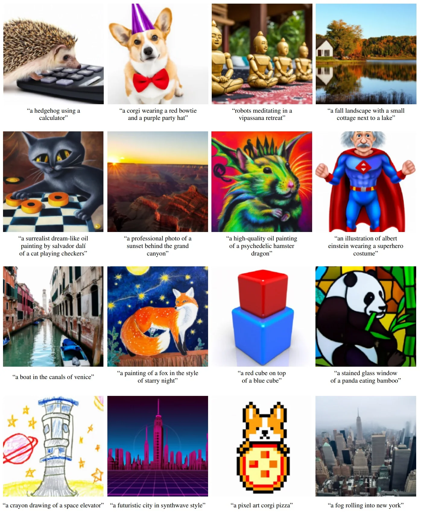
To condition on \( y \), GLIDE uses a frozen Transformer-based text encoder that converts the prompt into a sequence of contextual token embeddings. These embeddings are fused into the U-Net through cross-attention modules inserted at multiple spatial resolutions. This design enables the image representation at each location to selectively attend to different textual components, enforcing semantic alignment between visual structure and linguistic content. Two encoder variants are considered in the paper: a Transformer trained from scratch on image–text pairs, and the CLIP text encoder [512].
The objective used during training is a conditional variant of the DDPM noise prediction loss: \[ \mathcal {L}_{\mbox{GLIDE}} = \mathbb {E}_{x_0, \epsilon , t} \left [ \left \| \epsilon - \epsilon _\theta (x_t, t, y) \right \|^2 \right ], \] where the model learns to denoise \( x_t \) using both temporal and semantic information. This conditional learning setup allows GLIDE to support tasks like text-to-image synthesis, inpainting, and semantic image editing with a unified architecture.
As seen in Figure 20.71, GLIDE generalizes beyond literal training examples, demonstrating strong compositional ability and visual realism. This is made possible by its tight fusion of image-space diffusion and language semantics via cross-attention, allowing for rich conditional control.
Text Conditioning via Cross-Attention in GLIDE
In GLIDE [464], natural language prompts are embedded using a frozen Transformer encoder, which maps the input caption \( y \) into a sequence of contextualized token embeddings: \[ y \longmapsto \left \{ \mathbf {e}_1, \dots , \mathbf {e}_L \right \}, \qquad \mathbf {e}_i \in \mathbb {R}^d. \] Each vector \( \mathbf {e}_i \) captures the meaning of a specific token (word or subword) in context—e.g., the vector for “dog” will be different in “a dog” versus “hot dog.” The full sequence \( \{ \mathbf {e}_i \} \) thus encodes the semantics of the entire caption.
To inject this textual information into the image generation process, GLIDE modifies the self-attention mechanism inside the U-Net with cross-attention, where visual features act as queries and the text embeddings as both keys and values. At each attention block, the model computes: \[ \mbox{Attn}(Q, K, V) = \mathrm {softmax} \left ( \frac {Q K^\top }{\sqrt {d}} \right ) V, \] where: \[ Q = W_Q f, \quad K = W_K e, \quad V = W_V e. \]
- \( f \in \mathbb {R}^{H \times W \times c} \): the current spatial feature map from the U-Net, flattened to shape \( (HW, c) \) and linearly projected to form queries \( Q \in \mathbb {R}^{HW \times d} \).
- \( e \in \mathbb {R}^{L \times d} \): the caption token embeddings (from the text encoder), projected to keys \( K \in \mathbb {R}^{L \times d} \) and values \( V \in \mathbb {R}^{L \times d} \).
Why this works:
- The query vector \( Q_i \) at each image location \( i \) specifies a directional probe: it ”asks” which text tokens are most semantically relevant to what the model is generating at that pixel or patch.
- The dot-product \( Q_i K_j^\top \) measures the alignment between image location \( i \) and text token \( j \). The softmax turns this into a probability distribution over tokens—effectively letting each image region focus on specific language concepts.
- The final attended feature is a weighted combination of the value vectors \( V_j \), which carry semantic context from the caption and allow the image generator to access and integrate that information.
This structure allows the model to learn that, for example, when the caption includes “a dog in a red hat,” the spatial regions depicting the hat should align with the embedding for “hat,” and the dog’s body with “dog.” No token is “highlighted” in isolation—instead, relevance emerges dynamically as a function of the image context via learned query-key similarity.
This cross-modal alignment is applied at multiple resolutions within the U-Net, ensuring that text guidance is accessible across coarse layouts and fine details. The conditioning is thus not a global label but a dynamic, token-wise modulation of image generation grounded in semantic correspondence between modalities.
GLIDE’s Multi-Stage Generation Pipeline: A Cascaded Diffusion Strategy
GLIDE [464] employs a cascaded diffusion approach to synthesize high-resolution images from text prompts. It holds a similar intuition to the one behind Cascaded Diffusion Models (CDMs) [234], that we’ve previously covered (Enrichment 20.9.4), only this time it is based on a text encoding and not a class encoding. GLIDE divides the generation task into multiple stages, each operating at a different spatial resolution. This staged architecture improves quality and efficiency by allowing each model to focus on a specific aspect of the generation process.
- Base diffusion model (64\(\times \)64): A text-conditioned DDPM generates low-resolution \( 64 \times 64 \) images from captions. It captures coarse global structure, composition, and semantic alignment with the prompt. Operating at a small scale allows for training on large and diverse datasets.
- Super-resolution model (64\(\to \)256): A second diffusion model performs resolution upsampling. It takes as input a bilinearly upsampled version of the base output and the same text embedding. Conditioned on both, it synthesizes a \( 256 \times 256 \) image with finer visual details while preserving the semantic intent.
- (Optional) Final upsampler (256\(\to \)512): An optional third-stage model further increases resolution and sharpness, generating high-fidelity \( 512 \times 512 \) images. This stage is particularly useful in domains requiring photorealism or precise detail.
Why use cascading? GLIDE’s design is consistent with the principles of cascaded diffusion:
- Modularity and separation of concerns: The base model handles semantic composition and spatial layout. Super-resolution stages specialize in refining texture, edges, and fine-grained detail. This decomposition simplifies the learning objective at each stage.
- Improved sample quality: Errors and ambiguities in early low-resolution predictions can be corrected at higher resolutions through guided refinement.
- Efficiency: Lower-resolution generation requires fewer parameters and less computation. Later stages can reuse a smaller amount of training data focused on resolution pairs.
Each stage is trained independently. The super-resolution models are trained on paired low- and high-resolution crops, conditioned on both the image and the shared frozen text encoder. This encoder ensures that semantic alignment with the prompt is preserved across all stages. Cross-attention is employed at multiple layers in the U-Net, aligning image regions with relevant textual concepts.
Super-Resolution Modules in GLIDE After producing a coarse sketch using the \( 64 \times 64 \) base model, GLIDE [464] refines the image through a sequence of independently trained super-resolution diffusion models, typically for the resolution upgrades \( 64 \!\to \! 256 \) and optionally \( 256 \!\to \! 512 \). Each stage is responsible for enhancing visual fidelity by introducing higher-frequency detail, guided by both the upsampled coarse image and the original text prompt.
Each super-resolution module follows a structured training process:
- The input is a low-resolution image \( x^{\mbox{low}} \), obtained by downsampling a high-resolution training image \( x^{\mbox{high}} \) from the dataset.
- This \( x^{\mbox{low}} \) is bilinearly upsampled to the target resolution (e.g., from \( 64 \!\to \! 256 \)).
- Gaussian noise is added to the upsampled image using the forward diffusion schedule for that resolution stage, yielding a noised version \( x_t \).
- The model is trained to denoise \( x_t \) toward the original high-resolution ground truth \( x^{\mbox{high}} \), conditioned on both the noisy image and the associated text prompt \( y \).
Crucially, the same image-caption pair \( (x^{\mbox{high}}, y) \) is used across all stages of the cascade:
- The base model learns to generate a \( 64 \times 64 \) approximation of \( x^{\mbox{high}} \) given \( y \).
- The first super-resolution model refines that to \( 256 \times 256 \), using the blurred/noised upsampled \( 64 \times 64 \) image and still supervising against the same \( x^{\mbox{high}} \).
- The second super-res model (optional) further refines toward \( 512 \times 512 \), again targeting the same \( x^{\mbox{high}} \), now upsampled and re-noised accordingly.
This architecture ensures that all models in the cascade are aligned on a common semantic and visual goal. While the inputs to each stage differ in resolution and noise level, the supervision target \( x^{\mbox{high}} \) and prompt \( y \) remain constant throughout. This coherence prevents semantic drift and enables precise refinement of the coarse image toward the intended final output.
All models share a frozen T5 encoder for text conditioning. The token embeddings \( \{ \vec {e}_1, \dots , \vec {e}_L \} \) produced by this encoder are injected via cross-attention at multiple U-Net layers, ensuring that every spatial region in the image remains grounded in the prompt throughout all diffusion steps.
By training each stage to recover the original high-resolution dataset image from progressively degraded inputs, GLIDE ensures that the final samples are not just upsampled blobs, but semantically faithful, high-fidelity images—each stage building upon and correcting the previous.
Relationship to Cascaded Diffusion Models (CDMs) GLIDE [464] and CDMs [234] both follow a multi-stage pipeline: a low-resolution base model generates coarse images that are progressively refined through super-resolution diffusion stages. While the overall architecture is similar, the two differ in how they encode conditioning and enforce robustness during upsampling.
-
Conditioning and Guidance:
- GLIDE is conditioned on natural language via a frozen T5 encoder and uses classifier-free guidance (CFG) at inference. During training, 10% of prompts are dropped, allowing the model to learn both conditional and unconditional denoising. CFG interpolates their predictions to enhance prompt alignment.
- CDMs are class-conditioned using learned label embeddings injected into all models. No classifier-based or classifier-free guidance is used—class identity is always provided directly to the network.
-
Robustness via Degraded Conditioning:
- Both models degrade the upsampled low-resolution image before denoising. GLIDE uses fixed methods such as Gaussian blur and BSR, whereas CDMs apply randomized degradations (e.g., blur, JPEG compression, noise) drawn from a corruption distribution. This conditioning augmentation is more formally defined in CDMs and proven essential through ablations.
Summary: GLIDE and CDMs both use resolution-specific diffusion stages. The key differences are GLIDE’s use of natural language prompts and classifier-free guidance, versus CDMs’ reliance on class labels and stronger, randomized conditioning augmentation to maintain sample fidelity without external guidance.
Full Generation Pipeline of GLIDE
- 1.
- Base Diffusion Model (\( 64 \times 64 \)): A text-conditioned U-Net is trained using noise prediction loss to generate low-resolution samples that reflect the coarse layout and semantic intent of the prompt.
- 2.
- First Super-Resolution Stage (\( 64 \!\to \! 256 \)): The base image is upsampled and then re-noised. A second diffusion model is trained to remove the noise, refining texture, geometry, and visual coherence.
- 3.
- Optional Final Upsampler (\( 256 \!\to \! 512 \)): A third model further improves fidelity, handling fine details and photorealistic rendering. This model is trained with similar supervision but may use deeper architecture or stronger regularization.
Each model in the pipeline operates independently. All are conditioned on the same frozen T5 embeddings to ensure semantic consistency. Cross-attention is applied at various U-Net layers, so spatial features in the image are explicitly guided by token-level prompt information.
ADM U-Net Architecture in GLIDE The architecture of GLIDE [464] is built upon the ADM U-Net backbone introduced by Dhariwal and Nichol [123]. This network serves as the core denoising model at each stage of the diffusion cascade. While its layout resembles the canonical U-Net (see enrichment §15.6 and Figure [fig]), the ADM version integrates time and text conditioning, residual connections, and attention mechanisms in a more structured and scalable way.
Overall Structure. The U-Net processes a noisy input image \( x_t \in \mathbb {R}^{3 \times H \times W} \), a diffusion timestep \( t \), and a text prompt \( y \). The network is divided into three main components:
- Encoder path (downsampling): Each spatial resolution level includes two residual blocks and, optionally, a self-attention module. Downsampling is performed via strided convolutions, and the number of channels doubles after each resolution drop (e.g., 192 \( \to \) 384 \( \to \) 768).
- Bottleneck: At the lowest spatial resolution (e.g., \( 8 \times 8 \)), the model uses two residual blocks and one self-attention layer. This is where global semantic context is most concentrated.
- Decoder path (upsampling): This path mirrors the encoder. Each upsampling level includes residual blocks and optional self-attention, followed by nearest-neighbor upsampling and a \( 3 \times 3 \) convolution. Skip connections from the encoder are concatenated or added to the decoder at each level to preserve fine-grained detail.
Timestep Conditioning. The scalar diffusion timestep \( t \in \{0, \dots , T\} \) is encoded into a high-dimensional vector via sinusoidal embeddings, similar to the Transformer [664].
This vector is passed through a learnable MLP and injected into each residual block via FiLM-style modulation: \[ \mathrm {GroupNorm}(h) \cdot \gamma (t) + \beta (t), \] where \( \gamma (t), \beta (t) \in \mathbb {R}^d \) are scale and shift vectors derived from the timestep embedding, and \( h \) is the normalized activation.
Text Conditioning via Cross-Attention. The text prompt \( y \) is encoded using a frozen T5 encoder, yielding contextualized token embeddings \( \{ \vec {e}_1, \dots , \vec {e}_L \} \), with \( \vec {e}_i \in \mathbb {R}^d \). These are injected into the network via cross-attention in all attention layers. Each attention block computes: \[ \mathrm {Attn}(Q, K, V) = \mathrm {softmax}\left ( \frac {Q K^\top }{\sqrt {d}} \right )V, \] where: \[ Q = W_Q f, \quad K = W_K e, \quad V = W_V e, \] and \( f \in \mathbb {R}^{H \times W \times c} \) is the image feature map at that layer. This mechanism allows each spatial location in the image to query relevant semantic concepts from the caption.
Implementation Highlights. Key components of GLIDE’s U-Net implementation (adapted from glide_text2im/unet.py) include:
- Residual Blocks: All convolutional layers are embedded in residual units with FiLM-style conditioning and GroupNorm. Timestep embeddings and global pooled text embeddings are both added before nonlinearity.
- Attention Layers: Multi-head attention modules are inserted at intermediate resolutions (e.g., \( 64 \times 64 \), \( 32 \times 32 \), \( 16 \times 16 \)), depending on the stage (base model or super-resolution).
- Resolution Schedule: The base model uses four resolution levels with channel multipliers \([1, 2, 4, 4]\). Each resolution contains two residual blocks and an optional attention block. The total number of attention heads and layer width increases with resolution depth.
- Skip Connections: As in traditional U-Nets, skip connections copy activations from encoder layers to their corresponding decoder layers, enhancing spatial fidelity and stability during training.
Final Output. The decoder outputs a tensor \( \hat {\epsilon }_\theta (x_t, t, y) \in \mathbb {R}^{3 \times H \times W} \), representing the predicted noise. This estimate is used in the reverse diffusion step to move from \( x_t \to x_{t-1} \), progressively denoising toward the final image.
Summary of the GLIDE System GLIDE implements an early form of cascaded diffusion generation with the following key elements. It employs a text-conditioned U-Net backbone trained to synthesize low-resolution semantic content. It uses cross-attention mechanisms to maintain semantic alignment between the prompt and evolving image features. It applies a hierarchical cascade of independently trained super-resolution modules to improve fidelity and texture. This design enables scalable, prompt-consistent generation of high-resolution images without requiring auxiliary classifiers, external guidance models, or re-ranking. GLIDE’s architecture thus laid the foundation for subsequent cascaded frameworks, while demonstrating strong generalization across a wide range of text prompts and visual concepts.
Text-Guided Editing and Inpainting Capabilities Beyond pure text-to-image generation, one of GLIDE’s key contributions is its ability to perform conditional editing and inpainting through partial noising and constrained denoising steps. By erasing selected regions of an image, injecting Gaussian noise, and conditioning on both the surrounding pixels and a new text prompt, the model plausibly fills in missing content that respects the original style and semantics.
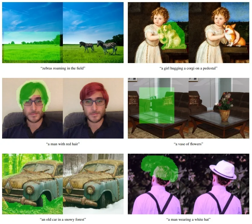
As shown in Figure 20.72, GLIDE performs image inpainting by conditioning the generative process on both a masked image and a guiding text prompt. To enable this capability, the model is fine-tuned specifically for inpainting using a dataset of partially masked images. During training, the model receives images with random rectangular regions removed and learns to denoise these masked regions while keeping the unmasked content fixed.
At inference time, the masked region is initialized with noise and updated using the standard diffusion sampling loop, while the known pixels are clamped to their original values at each step. This partial denoising scheme ensures that the generated content blends smoothly with the unmasked surroundings and adheres to the text condition.
Compared to GAN-based inpainting—which often requires adversarial losses and may fail to maintain semantic or spatial coherence—GLIDE leverages the stability and flexibility of its probabilistic denoising framework. The iterative nature of diffusion helps preserve global structure and yields completions that are both context-aware and text-consistent. Techniques such as classifier-free guidance can be retained during inpainting to further improve alignment with the prompt.
This mechanism also enables iterative refinement, wherein users can repeatedly mask regions, update the text prompt, and reapply the model to incrementally build complex scenes.
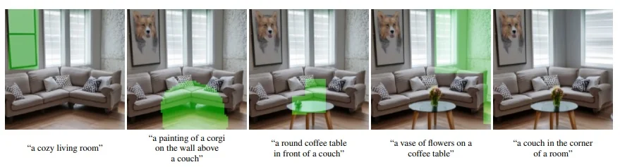
These capabilities demonstrate that GLIDE functions not just as a generator but as a flexible and interactive system for creative image manipulation. Its strength lies in preserving spatial coherence, semantic relevance, and stylistic fidelity across multiple user-guided editing stages.
Sketch-Based Conditional Editing with SDEdit GLIDE’s diffusion-based formulation enables an additional editing mode: sketch-to-image synthesis. By combining partial image inputs with language prompts, users can guide the model using both structure and semantics. This is achieved using a variant of Score-Based Generative Modeling known as SDEdit [434], which allows starting from a partially structured input and denoising it toward a visually coherent result.
In this setup, a user provides a crude input sketch or image fragment, alongside a prompt describing the desired output. The sketch is partially noised using the forward diffusion process (e.g., for 50 steps), and then the model is used to denoise it conditioned on the prompt. This ensures that the final image aligns with both the provided sketch and the semantic intent of the text.
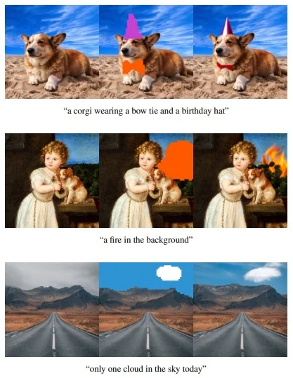
As illustrated in Figure 20.74, this hybrid mode yields outputs that respect the geometric intent of the sketch while capturing nuanced prompt attributes (e.g., color, material, object integration). Because using this technique in this setup builds directly on GLIDE’s denoising framework, it remains versatile and general-purpose—capable of tasks like edge-to-image rendering, stroke-based painting, and compositional sketching.
This functionality bridges the gap between hand-drawn control and natural language generation, offering a compelling example of multimodal guidance in diffusion systems.
Classifier-Free Guidance vs. CLIP Guidance GLIDE introduces two competing strategies for aligning image generation with a textual prompt: CLIP guidance and classifier-free guidance (CFG). While both aim to steer the sampling trajectory toward semantic fidelity, they differ significantly in implementation, stability, and perceptual outcomes.
CLIP guidance [512] optimizes the cosine similarity between image and text embeddings produced by a frozen CLIP model: \[ \max _x \; \cos \left ( f_{\mbox{CLIP}}(x), f_{\mbox{CLIP}}(y) \right ). \] This gradient-based alignment is applied across the diffusion trajectory, encouraging denoised latents \( x_t \) to resemble images that CLIP deems semantically close to the prompt \( y \). While conceptually direct, this approach has several drawbacks:
- Gradient mismatch: CLIP is trained on fully denoised, high-quality images, whereas diffusion models operate over progressively noised latents. Applying CLIP’s gradients to noisy intermediate states introduces distributional mismatch, often steering the denoising trajectory off-manifold and resulting in unstable generation.
- Adversarial artifacts: Because CLIP is used both to guide and to evaluate image quality, the generative model may exploit weaknesses in CLIP’s embedding space. Instead of faithfully representing the prompt, it may synthesize images that trick CLIP into assigning high similarity scores—despite the samples being visually implausible or semantically incoherent to humans. This adversarial overfitting is particularly severe at high guidance scales, where the generator over-optimizes for CLIP alignment and produces unnatural textures or distorted compositions that ”hack” the metric.
- Tuning sensitivity: Effective use of CLIP guidance requires delicate balancing of the gradient scale. Weak guidance may yield vague or off-target generations, while overly strong guidance often causes prompt overfitting, repetitive artifacts, or structural collapse—manifesting as over-sharpened or corrupted outputs.
To partially address these limitations, GLIDE also experimented with a noised CLIP variant trained on corrupted images. While this reduced mismatch at early timesteps, it did not eliminate instability or the reliance on external model supervision.
Classifier-free guidance (CFG) [233], by contrast, is fully embedded into the model’s training objective. During training, the model randomly receives either a full prompt \( y \) or an empty (null) prompt \( \varnothing \), enabling it to learn both conditional and unconditional behaviors. At inference, these predictions are interpolated to amplify prompt fidelity: \begin {equation} \epsilon _{\mbox{CFG}} = \epsilon _\theta (x_t, t, \varnothing ) + s \cdot \left ( \epsilon _\theta (x_t, t, y) - \epsilon _\theta (x_t, t, \varnothing ) \right ), \end {equation} where \( s \geq 1 \) is the guidance scale.
CFG is simple, robust, and model-native. It requires no additional networks or loss terms, introduces no adversarial gradient pathways, and scales gracefully across prompts and domains. Although guidance inevitably reduces output diversity, GLIDE shows that CFG manages the fidelity–diversity trade-off more favorably than CLIP guidance. While CLIP guidance aggressively sacrifices variation to maximize alignment scores, CFG maintains perceptual quality without mode collapse.
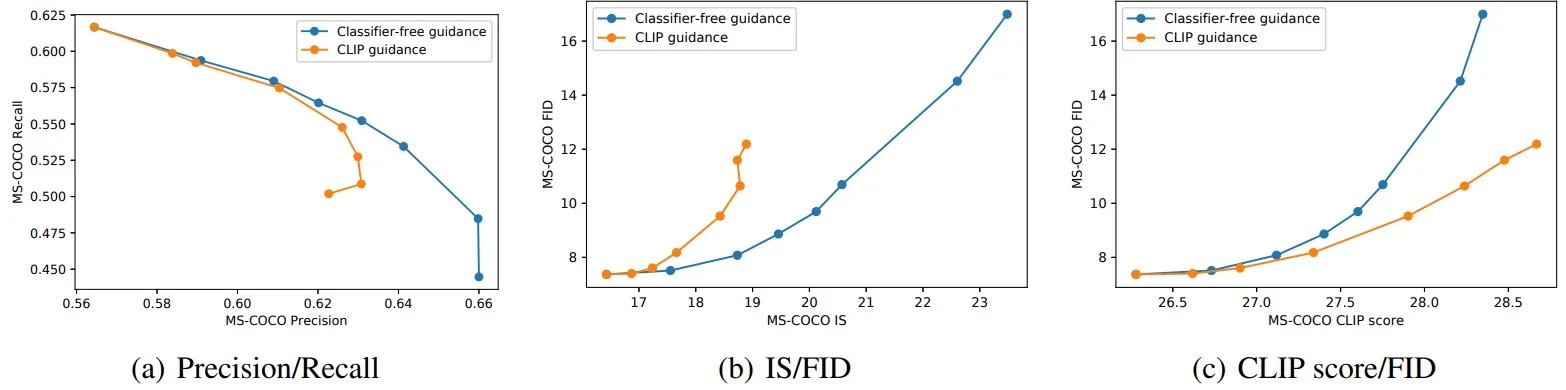
This superiority is reflected in human preference studies. GLIDE uses Elo scoring—a rating system adapted from competitive games like chess—to compare pairs of samples from different guidance methods. Each approach accumulates points based on relative preference in head-to-head matchups.
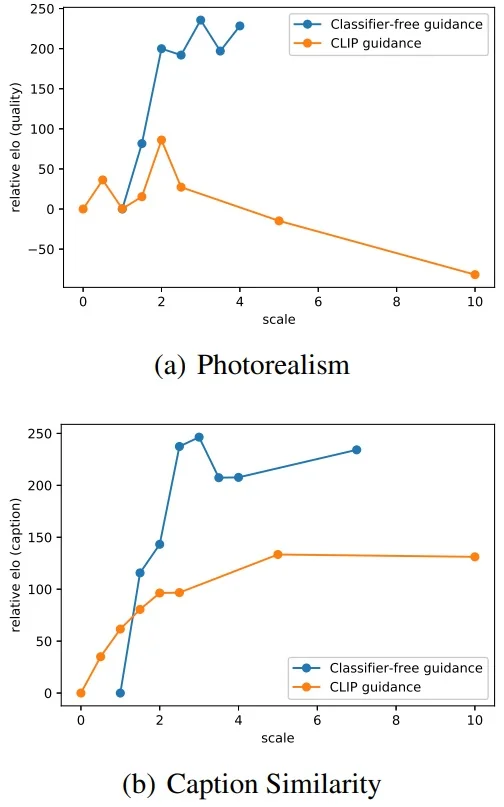
Takeaway: Classifier-free guidance is a foundational technique for modern diffusion-based image generation. It integrates directly with the model’s architecture, avoids adversarial gaming of external metrics, and produces samples that are consistently favored by human evaluators. Its success in GLIDE set the stage for adoption in subsequent systems like Stable Diffusion [548], Imagen [557], and Parti [765].
Failure Cases and Architectural Limitations Despite its strong generative capabilities, GLIDE exhibits clear limitations when tasked with abstract reasoning, rare object compositions, or spatially intricate prompts. Failure cases include implausible geometries (e.g., “a car with triangular wheels”), semantic mismatches (e.g., “a mouse hunting a lion”), and weak attribute binding. Figure 20.77 illustrates such inconsistencies in spatial relationships, object placement, and compositional coherence.
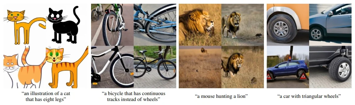
These challenges stem, in part, from GLIDE’s architectural design. The model operates directly in pixel space using a cascade of resolution-specific diffusion U-Nets, from a \(64 \times 64\) base model to higher-resolution super-resolution modules. While this cascade enables high-fidelity output, it incurs significant computational cost and can propagate or amplify local inconsistencies—especially when text conditioning is vague or underspecified.
Text conditioning in GLIDE is injected via frozen T5 embeddings applied through cross-attention at each U-Net layer. While effective for common prompts, this mechanism is static and may fail to capture fine-grained semantics, particularly in rare or compositional settings. Attempts to enhance conditioning using CLIP guidance led to brittle behavior: though CLIP gradients improved prompt alignment metrics, they also introduced adversarial artifacts and degraded visual plausibility [464]. Even a noise-aware CLIP variant, trained on noised latents, did not eliminate these issues.
In contrast, classifier-free guidance (CFG) [233] proved more robust, offering sharper, more coherent samples while maintaining a reasonable fidelity–diversity trade-off. Still, GLIDE’s monolithic design entangles semantic interpretation and pixel-level synthesis in a single forward trajectory, limiting the model’s controllability and generalization to atypical prompts.
These limitations motivated a shift in architecture. Rather than generating images directly from text in pixel space, DALL·E 2 (also known as unCLIP) proposes a modular framework that decouples semantic modeling from image generation. The design consists of:
- A pretrained CLIP encoder that embeds the text prompt into a dense latent space.
- A prior model—either autoregressive or diffusion-based—that maps the text to plausible CLIP image embeddings \( \vec {z}_i \).
- A diffusion decoder that generates the final image conditioned on \( \vec {z}_i \) (and optionally the original text).
This two-stage pipeline enables specialization: the prior operates in CLIP’s compact semantic space, improving prompt generalization and sample diversity, while the decoder focuses purely on photorealistic rendering.
Unlike GLIDE, guidance does not collapse diversity in unCLIP, since semantic information is already embedded in \( \vec {z}_i \) and remains fixed during decoding [524]. As we will see, this architectural decoupling resolves several of GLIDE’s bottlenecks and introduces new capabilities—such as zero-shot image editing and text-guided variations.
Before introducing DALL·E 2 in depth, we briefly revisit its predecessor—DALL·E 1 [525]—which pioneered large-scale text-to-image synthesis using discrete visual tokens and an autoregressive transformer. Although limited in resolution and editability, DALL·E 1 established key ideas—such as VQ-VAE bottlenecks and joint modeling of image and text tokens—that laid the groundwork for modern generative systems.
Enrichment 20.11.2: DALL·E 1: Discrete Tokens for Text-to-Image Generation
Motivation: Turning Images into Token Sequences for GPT-Style Modelling DALL\(\cdot \)E 1 [525] reframes text-to-image generation as conditional autoregressive sequence modeling. Inspired by the success of GPT-3 [58], which generates fluent text by predicting one token at a time, DALL\(\cdot \)E extends this idea to vision: if an image can be represented as a sequence of discrete tokens, then a transformer could learn to ”write” images one token at a time, conditioned on a caption.
Applying GPT-style architectures directly to pixels is infeasible for two key reasons:
- Memory constraints: A \( 256 \times 256 \) RGB image contains nearly 200,000 pixel values, far exceeding the context length supported by transformers with quadratic self-attention.
- Low-level fidelity bias: Pixel-wise likelihoods encourage matching short-range visual details but are poor at capturing global semantic structure aligned with a text prompt.
To address these issues, DALL\(\cdot \)E adopts a two-stage pipeline:
- 1.
- Stage A — Discrete Visual Tokenization (VQ-VAE).
A Vector-Quantized Variational Autoencoder (VQ-VAE) is trained to compress and reconstruct images. Specifically:- The encoder downsamples a \( 256 \times 256 \) RGB image into a \( 32 \times 32 \) latent grid.
- Each latent vector is replaced with the nearest of \( K = 8192 \) codebook entries, producing a discrete token map \( z \in \{1, \dots , K\}^{32 \times 32} \).
- The decoder reconstructs the image from these discrete codes using nearest-neighbor embeddings.
After training, both the encoder and decoder are frozen. They serve distinct roles:
- The encoder is used to tokenize training images into fixed-length sequences of visual indices.
- The decoder is used at inference time to reconstruct the final image from the predicted image tokens.
- 2.
- Stage B — Transformer-Based Sequence Modeling.
Once the image-token vocabulary is defined by the VQ-VAE, DALL\(\cdot \)E trains a decoder-only Transformer to model the conditional distribution over joint text–image token sequences. The training input is a single, flattened sequence: \[ \underbrace {\mbox{[BPE-encoded caption tokens]}}_{\mbox{text context}} \;\|\; \underbrace {\mbox{[VQ-VAE image tokens]}}_{\mbox{target to predict}}, \] where || denotes concatenation. The model autoregressively learns to predict the next token given all previous ones, using a standard maximum likelihood objective.At inference time, the generation process unfolds in three main steps:
- (a)
- The input caption is tokenized using Byte Pair Encoding (BPE).
- (b)
- The Transformer autoregressively generates a sequence of 1024 discrete image tokens—each corresponding to a \( 32 \times 32 \) position in the image grid.
- (c)
- These image tokens are passed to the frozen VQ-VAE decoder, which transforms them into a full \( 256 \times 256 \) RGB image.
This stage completes the pipeline: the Transformer acts as a powerful prior over visual token sequences, and the VQ-VAE decoder serves as the renderer that translates discrete tokens into pixel-level images. The reuse of pretrained components ensures modularity, while the tokenized format enables the Transformer to operate over images in exactly the same way it operates over language—token by token.
This design turns the image generation task into a symbolic language modeling problem. By discretizing images, DALL\(\cdot \)E enables the reuse of scaling laws, architectures, and optimization methods originally developed for large language models. The VQ-VAE bottleneck plays a critical role: it reduces the transformer’s sequence length by a factor of 192, enforces a visual vocabulary, and allows the image generator to focus on semantic structure rather than low-level pixel precision.
Why not use a Vision Transformer (ViT) instead of a VQ-VAE? At the time of DALL\(\cdot \)E 1’s development (early 2020), ViT-style self-supervised encoders (e.g., SimCLR, BYOL, MAE) were not yet mature enough to support discrete symbolic modeling.
Could a ViT-style encoder work today? Yes—modern systems like VQ-GAN [149], MAE [219], and DALL\(\cdot \)E 2 combine transformer or CLIP-style features with either residual quantization or diffusion decoders. Advances in scalable mixed-precision training and robust quantization make ViT-based latent spaces viable. Later parts in this book revisit these improved architectures.
In summary, DALL\(\cdot \)E 1’s symbolic bottleneck—powered by a convolutional VQ-VAE—offered a compact, expressive, and discrete latent space for training GPT-style transformers over images. While ViT-based alternatives have since become popular, the VQ-VAE’s combination of discrete representation, efficient decoding, and architectural maturity made it the most practical choice at the time.
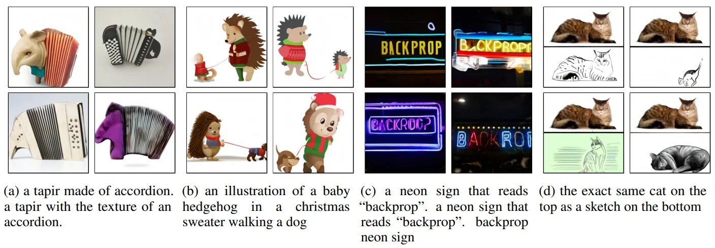
How VQ-VAE Enables Discrete Tokenization The tokenizer in DALL·E 1 [525] is based on a vector-quantized variational autoencoder (VQ-VAE), which converts high-resolution images into grids of discrete latent tokens. Specifically, it maps each \( 256 \times 256 \) RGB image into a \( 32 \times 32 \) grid, where each element indexes one of \( K = 8192 \) codebook vectors. These indices serve as compact image tokens for downstream modeling.
Training the Discrete VAE in DALL\(\cdot \)E 1. The VQ-VAE tokenizer used in DALL\(\cdot \)E 1 [525] maps high-resolution input images into a grid of discrete latent tokens, enabling downstream modeling with autoregressive transformers.
During training, the encoder processes the input image and outputs a spatial grid of logits \( \boldsymbol {\ell }_{i,j} \in \mathbb {R}^K \), where \( K \) is the number of codebook vectors and \( (i,j) \) indexes the spatial position in the latent map. These logits represent unnormalized log-probabilities over the discrete latent variables. A softmax is applied to yield a categorical distribution: \[ p_{i,j}(k) = \mbox{softmax}(\boldsymbol {\ell }_{i,j})_k, \] which defines the probability of selecting the \( k \)-th codebook vector at location \( (i,j) \).
Since sampling discrete indices is non-differentiable, the model applies the Gumbel-softmax relaxation [272] to enable end-to-end training. This technique approximates categorical sampling using a continuous, differentiable proxy. Instead of selecting a single index, the encoder produces a convex combination of the codebook vectors: \[ \vec {z}_{i,j} = \sum _{k=1}^K p_{i,j}(k) \cdot \vec {e}_k, \] where \( \vec {e}_k \in \mathbb {R}^d \) is the \( k \)-th learned codebook embedding. The resulting latent grid \( \{ \vec {z}_{i,j} \} \) is passed to the decoder, which attempts to reconstruct the original image.
The VQ-VAE in DALL\(\cdot \)E 1 is trained to maximize the Evidence Lower Bound (ELBO) on the log-likelihood of the data distribution. This objective consists of two terms:
-
Reconstruction loss: This term encourages the decoder to faithfully reconstruct the input image from its latent representation. During training, the decoder receives a softly quantized grid of latent vectors \( \vec {z} = \{ \vec {z}_{i,j} \} \), obtained via Gumbel-softmax relaxation over the encoder’s logits. The decoder outputs a reconstructed image \( \hat {x} = D_\theta (\vec {z}) \), which is compared to the original input \( x \).
The reconstruction loss assumes an isotropic Gaussian likelihood with unit variance at each pixel. This leads to a negative log-likelihood that simplifies to pixel-wise mean squared error (MSE): \[ \mathcal {L}_{\mbox{recon}} = \mathbb {E}_{x \sim \mathcal {D}} \left [ \left \| x - D_\theta (\vec {z}) \right \|_2^2 \right ]. \] Although MSE does not capture perceptual similarity (e.g., sensitivity to spatial misalignments or texture), it provides dense gradient feedback that encourages the encoder to preserve low-level spatial and textural details. These local features—edges, contours, and color regions—are crucial for producing discrete token sequences that retain semantic and structural information required by the downstream transformer.
More perceptually aligned metrics such as LPIPS [800] are often used in tasks that prioritize human visual judgment, but are computationally more intensive and less stable in early training. In contrast, MSE offers simplicity, efficiency, and sufficient structural fidelity for the purposes of compression and symbolic modeling.
-
KL divergence regularization: At each spatial location \( (i,j) \), the encoder outputs a categorical distribution \( p_{i,j}(k) \) over the \( K \) codebook entries. To discourage codebook collapse—a failure mode where only a small subset of the codebook is consistently used—the model includes a regularization term that penalizes deviation from a uniform prior: \[ \mathcal {L}_{\mbox{KL}} = \sum _{i,j} \mathrm {KL} \left [ p_{i,j}(k) \,\|\, \mathcal {U}(k) \right ], \] where \( \mathcal {U}(k) = \frac {1}{K} \) denotes the uniform categorical distribution over all \( K \) codebook entries.
This KL term encourages the encoder to distribute probability mass more evenly across the entire codebook. Without such regularization, the model may converge to using only a small number of tokens—those that are easiest for the decoder to reconstruct—thereby underutilizing the available representational capacity. This phenomenon, known as codebook collapse, reduces expressiveness and limits the diversity of visual patterns that the latent space can encode.
The uniform prior \( \mathcal {U}(k) \) reflects a modeling assumption that, across the dataset, all codebook entries should be equally likely. While this may not hold exactly in practice, it serves as a useful tool: by nudging the encoder’s output distributions \( p_{i,j}(k) \) closer to uniform, the model is encouraged to explore and specialize different code vectors. This improves latent diversity and makes the discrete token space more informative for downstream components such as autoregressive transformers.
The final objective function optimized during training is the ELBO: \[ \mathcal {L}_{\mbox{ELBO}} = \mathcal {L}_{\mbox{recon}} + \beta \cdot \mathcal {L}_{\mbox{KL}}, \] where \( \beta \) is a tunable hyperparameter that governs the trade-off between reconstruction fidelity and latent space regularization. A carefully chosen \( \beta \) ensures that the model learns discrete representations that are both structurally informative and uniformly distributed.
How is the codebook updated? Because the relaxed latent vector \( \vec {z}_{i,j} \) is a weighted average over the codebook entries, and the decoder is fully differentiable, the reconstruction loss induces gradients with respect to the codebook vectors \( \vec {e}_k \). These vectors are updated directly through backpropagation, with each one receiving a contribution proportional to its selection probability \( p_{i,j}(k) \) across spatial locations. This continuous relaxation allows efficient training of the discrete bottleneck.
Why is this relaxation valid if inference uses argmax?
At inference time, each spatial location \( (i,j) \) is assigned a discrete codebook index using a hard argmax over the encoder logits: \[ z_{i,j} = \arg \max _k \boldsymbol {\ell }_{i,j}[k]. \] This produces a symbolic grid of tokens that the transformer processes as a sequence over a fixed vocabulary. Since transformer models operate exclusively over discrete categorical inputs, these hard assignments are necessary for compatibility with downstream autoregressive generation.
However, during training, the non-differentiability of argmax prevents gradients from propagating into the encoder and codebook. To enable end-to-end optimization, the model instead uses a Gumbel-softmax relaxation [272]—a differentiable approximation to categorical sampling. For each location \( (i,j) \), the encoder outputs logits \( \boldsymbol {\ell }_{i,j} \in \mathbb {R}^K \), which are perturbed with Gumbel noise and scaled by a temperature \( \tau > 0 \) to yield soft categorical probabilities: \[ p_{i,j}(k) = \frac {\exp \left ((\boldsymbol {\ell }_{i,j}[k] + g_k)/\tau \right )}{\sum _{k'=1}^{K} \exp \left ((\boldsymbol {\ell }_{i,j}[k'] + g_{k'})/\tau \right )}, \qquad g_k \sim \mbox{Gumbel}(0, 1). \]
Here, the Gumbel noise \( g_k \) serves a specific purpose: it injects stochasticity that simulates sampling from a categorical distribution while keeping the operation differentiable. In effect, it perturbs the logits just enough to allow a continuous approximation of discrete sampling. The softmax over noisy logits mimics drawing from a categorical distribution in expectation, but permits gradients to flow through the output probabilities \( p_{i,j}(k) \). Without this noise, the relaxation would simply reduce to a softmax over logits and lose the stochastic behavior necessary to model discrete sampling during training.
The latent vector is then computed as a convex combination of codebook entries: \[ \vec {z}_{i,j} = \sum _{k=1}^{K} p_{i,j}(k) \cdot \vec {e}_k, \] where \( \vec {e}_k \in \mathbb {R}^d \) is the \( k \)-th learned codebook embedding.
The temperature \( \tau \) plays a central role in this process: it controls the sharpness of the softmax. At high values, the output distribution is diffuse, placing weight on multiple entries. As \( \tau \to 0 \), the distribution becomes increasingly concentrated on the largest logit, approaching a one-hot vector. To reconcile soft training with hard inference, \( \tau \) is gradually annealed during training—typically down to \( \tau = \tfrac {1}{16} \). This causes the encoder’s soft outputs to become sharply peaked, closely approximating the behavior of argmax by the end of training.
As a result, the decoder—trained on these increasingly sharp latent vectors—becomes robust to the true hard tokens it will encounter at test time. Meanwhile, a KL divergence term encourages the encoder to maintain high entropy across codebook usage, preventing mode collapse and promoting a rich, expressive latent space.
In summary, the Gumbel-softmax relaxation enables differentiable training by producing soft samples over codebook entries. The temperature parameter \( \tau \) controls how close these samples are to true one-hot vectors, while the Gumbel noise simulates discrete sampling in a smooth and trainable way. Together with annealing, reconstruction loss, and KL regularization, this mechanism allows the model to learn discrete latent codes that are both optimizable and fully compatible with transformer-based generation.
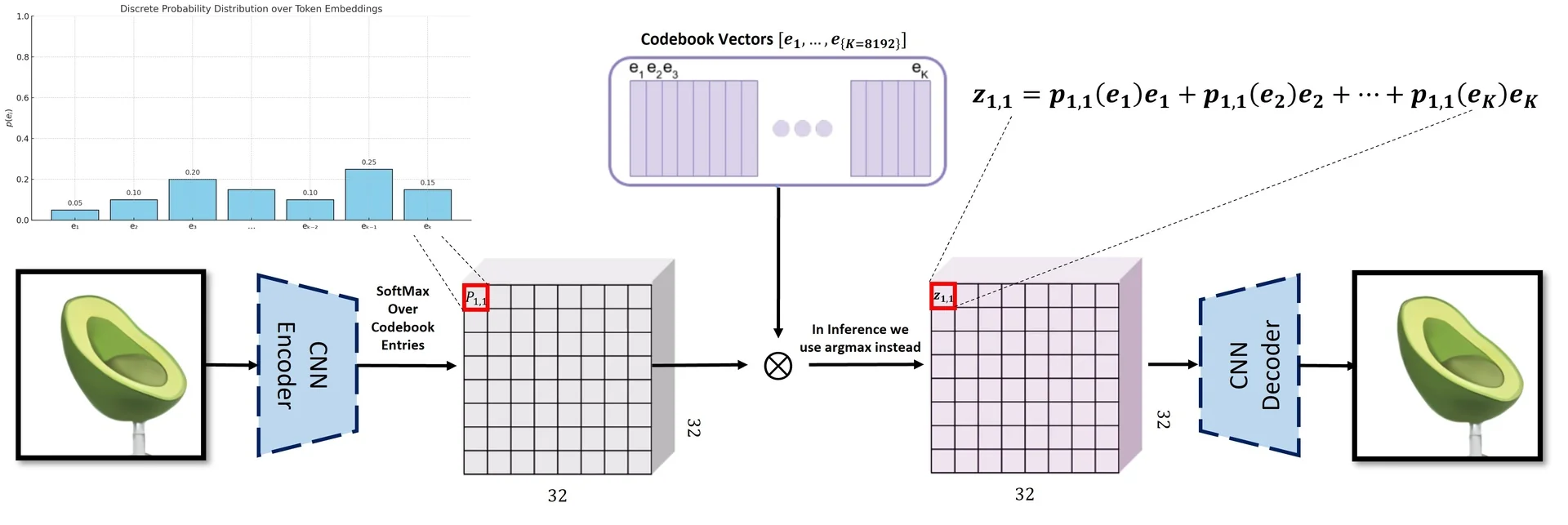
Note that while this simplification stabilizes training and integrates well with transformer-based generation, it comes at the cost of reduced discreteness. Each latent vector becomes a blend of multiple codebook entries rather than a single, clearly defined symbol. In contrast, models like VQ-VAE-2—though not designed to interface with transformers—use hard quantization to enforce strictly discrete representations. This is especially important in applications focused on compression, clustering, or symbolic reasoning, where each token must correspond to a well-defined and separable concept.
For instance, in tasks like class-conditional generation or latent space interpolation, soft assignments can blur distinct concepts (e.g., mixing “cat” and “dog” embeddings), leading to ambiguous representations. Hard assignments avoid this by ensuring each latent token corresponds to a single, interpretable codebook entry—even if training becomes more complex due to the non-differentiability of the quantization step.
Inference-Time Token Generation and Decoding
At inference time, DALL\(\cdot \)E 1 generates images directly from a text prompt—without any image input. The encoder of the VQ-VAE is bypassed entirely. Instead, the caption is first tokenized into a sequence of subword units using Byte Pair Encoding (BPE), which serves as context for a powerful decoder-only transformer. This transformer then autoregressively generates a sequence of 1024 discrete image tokens, each representing a codebook index in a \( 32 \times 32 \) spatial grid. Once the full token sequence is sampled, it is passed to the frozen VQ-VAE decoder to reconstruct a high-resolution \( 256 \times 256 \) RGB image.
- 1.
- The caption is tokenized into \( T_\mbox{text} \) BPE tokens: \( [x_1^{\mbox{text}}, \dots , x_{T_\mbox{text}}^{\mbox{text}}] \).
- 2.
- The transformer generates image tokens one by one: \[ x_{t}^{\mbox{image}} \sim p(x_t^{\mbox{image}} \mid x_1^{\mbox{text}}, \dots , x_{T_\mbox{text}}^{\mbox{text}}, x_1^{\mbox{image}}, \dots , x_{t-1}^{\mbox{image}}) \] for \( t = 1, \dots , 1024 \).
- 3.
- The resulting sequence is reshaped into a \( 32 \times 32 \) grid and decoded into pixels by the VQ-VAE decoder.
This architecture separates semantic generation from image rendering:
- The transformer serves as a semantic prior, generating a symbolic image consistent with the caption.
- The decoder acts as a neural renderer, translating discrete tokens into photorealistic pixel outputs.
Training the Transformer with Discrete Tokens
To enable text-to-image generation, the transformer is trained to model the joint distribution over text and image tokens: \[ p_\psi (\vec {x}^{\mbox{text}}, \vec {x}^{\mbox{image}}) = \prod _{t=1}^{T_\mbox{text} + 1024} p_\psi (x_t \mid x_1, \dots , x_{t-1}), \] where \( \vec {x}^{\mbox{text}} = [x_1^{\mbox{text}}, \dots , x_{T_\mbox{text}}^{\mbox{text}}] \) are the BPE-encoded caption tokens and \( \vec {x}^{\mbox{image}} = [x_1^{\mbox{image}}, \dots , x_{1024}^{\mbox{image}}] \) are the discrete image tokens derived from the VQ-VAE encoder via hard argmax quantization.
During training, these two sequences are concatenated into a single input: \[ [x_1^{\mbox{text}}, \dots , x_{T_\mbox{text}}^{\mbox{text}}, x_1^{\mbox{image}}, \dots , x_{1024}^{\mbox{image}}], \] and fed into the transformer, which is trained to predict each token in the sequence from its preceding context using a causal attention mask. The model performs next-token prediction across the entire sequence—first within the caption, then across the image region—with no distinction in architecture between the two parts.
Importantly, cross-modal conditioning arises naturally: since image tokens are positioned after the text tokens, they are allowed to attend to the entire caption. This enables the model to learn text-guided image synthesis within a unified autoregressive framework.
The loss function used is standard categorical cross-entropy over all tokens in the sequence: \[ \mathcal {L}_{\mbox{total}} = \sum _{t=1}^{T_\mbox{text}} \lambda _{\mbox{text}} \cdot \mathcal {L}_{\mbox{CE}}(x_t) + \sum _{t=T_\mbox{text}+1}^{T_\mbox{text}+1024} \lambda _{\mbox{image}} \cdot \mathcal {L}_{\mbox{CE}}(x_t), \] where \( \lambda _{\mbox{text}} \ll \lambda _{\mbox{image}} \) (typically \( \frac {1}{8} \) vs. \( \frac {7}{8} \)) to emphasize the importance of accurate image modeling. This bias reflects the downstream goal of generating images, not captions.
Additional regularization techniques—such as BPE dropout (which randomly alters token splits) and spatial attention priors over the image portion—are used to improve robustness and sample quality.
By training in this way, the transformer learns to interpret the caption as a prefix and generate a coherent visual token sequence conditioned on it. At inference time, the same structure is followed: given only a text prompt, the model samples tokens autoregressively to produce an image in the VQ-VAE’s discrete latent space.
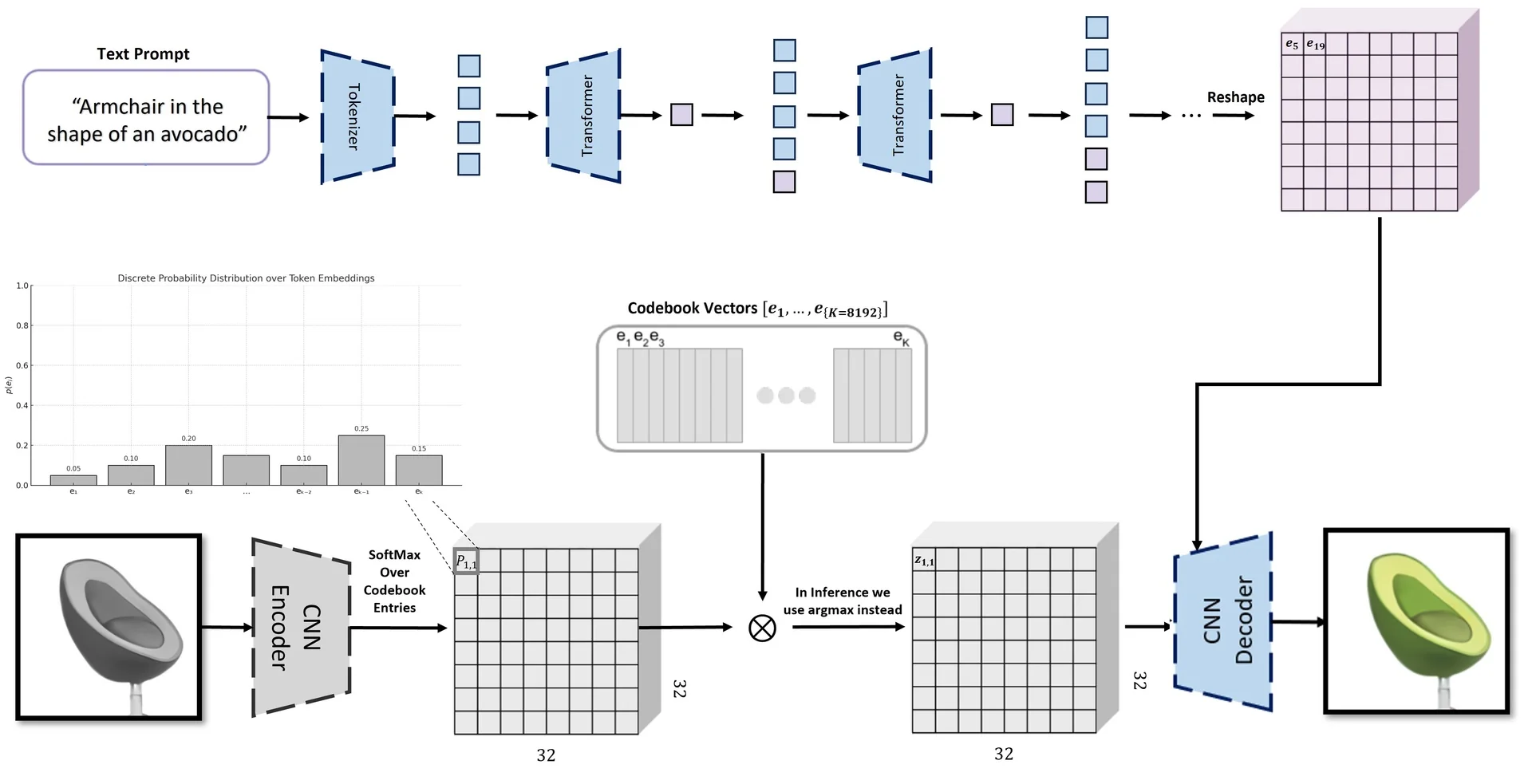
Clarifying Terminology: dVAE vs. VQ-VAE The DALL\(\cdot \)E paper uses the term discrete VAE (dVAE) to refer to its tokenizer, which is effectively a VQ-VAE trained with soft relaxation. While VQ-VAE-2 [530] adds hierarchical levels and is suited to pixel-space autoregression, DALL\(\cdot \)E uses only a flat VQ-VAE and does not employ VQ-VAE-2 or hierarchical latent modeling.
Training Datasets and Sample Generation Pipeline DALL\(\cdot \)E 1 is trained on a large-scale dataset comprising 250 million (text, image) pairs scraped from the internet. Captions are tokenized using Byte Pair Encoding (BPE), while corresponding images are compressed into \( 32 \times 32 \) grids of discrete tokens via a VQ-VAE encoder. This diverse and weakly supervised corpus exposes the model to a broad spectrum of concepts and modalities, enhancing its generalization to novel text prompts at inference time.
During image generation, after receiving a text prompt, DALL\(\cdot \)E 1 begins the process of autoregressively sampling a sequence of 1024 discrete image tokens using a decoder-only sparse transformer with 12 billion parameters. Although the model’s weights are fixed and deterministic after training, the decoding process at inference time is deliberately stochastic.
At each of the 1024 generation steps, the model outputs a logit vector \( \boldsymbol {\ell } \in \mathbb {R}^{8192} \), corresponding to a categorical distribution over the image vocabulary. Instead of applying greedy decoding (selecting the most likely token at each step), the model samples from this distribution. To modulate the diversity of outputs, it uses temperature-based sampling, a method confirmed in the original paper [525]. The logits are rescaled as: \[ \tilde {p}_k \propto \exp \left ( \frac {\ell _k}{\tau } \right ), \] where \( \tau > 0 \) controls the sharpness of the softmax distribution. For \( \tau = 1 \), the model samples directly from the raw distribution; lower \( \tau \) values sharpen the probabilities (favoring high-confidence tokens), while higher values flatten them (increasing randomness). The authors report results under different temperatures, including \( \tau = 0.85 \) and \( \tau = 1.0 \), showing that trade-offs between diversity and fidelity can be tuned via this parameter.
It is important to note that even with a fixed temperature, the process remains non-deterministic. The temperature shapes the distribution but does not determine the sampled outcome. At each step, the model draws from a distribution with nonzero entropy—akin to rolling a die with unequal probabilities. Thus, for a fixed prompt and temperature, different sequences can still emerge due to randomness in token sampling.
To generate a batch of \( N \) candidate images, this entire sampling process is simply repeated \( N \) times. Each run yields a distinct sequence of 1024 discrete image tokens, reflecting a unique plausible interpretation of the same input caption. The diversity across these sequences arises entirely from stochastic sampling—there is no injected model-level noise (such as dropout) at generation time.
Once generated, each of the \( N \) sampled token sequences is decoded into a full-resolution \( 256 \times 256 \) RGB image using the pretrained and frozen VQ-VAE decoder. These images form the candidate pool for the subsequent CLIP-based reranking phase.
To select the most relevant images from the candidate set, DALL\(\cdot \)E applies a contrastive reranking strategy using CLIP [512], a pretrained model that embeds both text and images into a shared semantic space. Each image is scored by computing the cosine similarity between its embedding and the embedding of the input caption. The top-ranked images—those most semantically aligned with the prompt—are selected as final outputs.
This two-stage pipeline—stochastic sampling followed by CLIP-based semantic reranking—enables DALL\(\cdot \)E to generate high-quality and semantically faithful images from diverse prompts. During sampling, diversity is promoted through temperature-based decoding; during reranking, relevance is enforced by scoring candidates against the caption using CLIP [512]. This separation of concerns allows the model to handle ambiguous or open-ended prompts effectively: by increasing the number of samples \( N \), it becomes more likely that one or more generations will match the intent of the caption.
However, this strategy comes at a significant computational cost. Generating \( N = 512 \) high-resolution image candidates requires 512 full autoregressive decoding passes through a 12-billion parameter transformer and subsequent VQ-VAE decoding—making the approach expensive in both time and memory. While effective for research and offline applications, this procedure may be less practical in low-latency or resource-constrained settings.
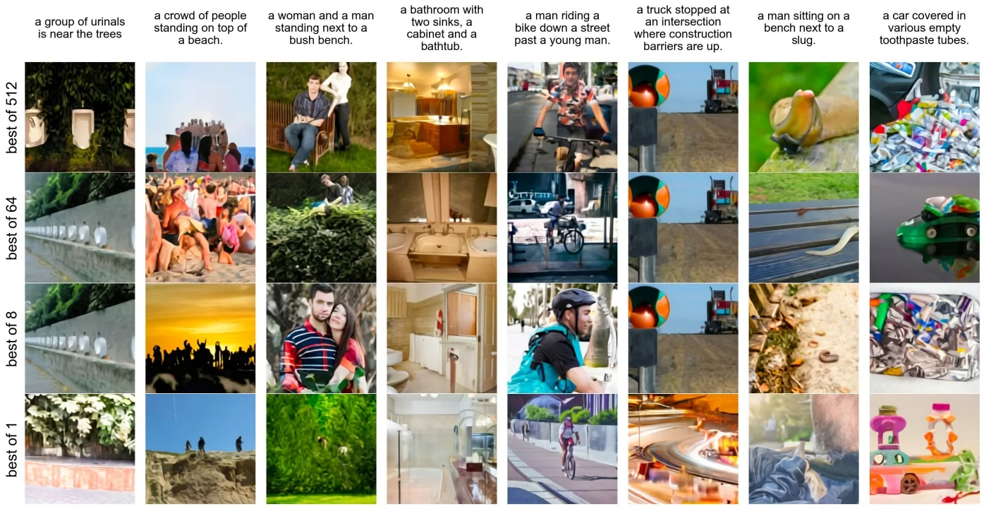
Experimental Results and Motivation for DALL\(\cdot \)E 2 DALL\(\cdot \)E 1 delivers impressive zero-shot image generation capabilities, establishing a strong baseline for symbolic text-to-image synthesis. On MS-COCO captions, its samples are consistently preferred by human raters over those from prior work (e.g., DF-GAN [628]). In a best-of-five vote, DALL\(\cdot \)E’s generations were judged more realistic 90% of the time and more semantically aligned with the caption 93.3% of the time. These results are particularly notable given that DALL\(\cdot \)E was evaluated in a zero-shot setting—without task-specific fine-tuning.
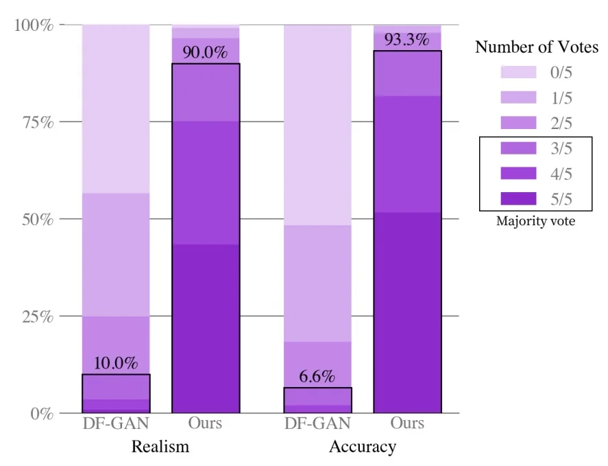
Quantitative benchmarks further validate these findings. On MS-COCO, DALL\(\cdot \)E achieves a Fréchet Inception Distance (FID) competitive with state-of-the-art models—within 2 points of the best prior approach—and outperforms all baselines when a mild Gaussian blur is applied to reduce decoder artifacts. Its Inception Score (IS) also improves under similar conditions. However, on more specialized datasets like CUB [672], DALL\(\cdot \)E’s performance drops sharply, with a nearly 40-point FID gap between it and task-specific models. This limitation is visually evident in the model’s CUB generations: while bird-like in appearance, they often lack anatomical consistency and fine-grained control.
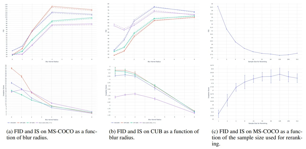
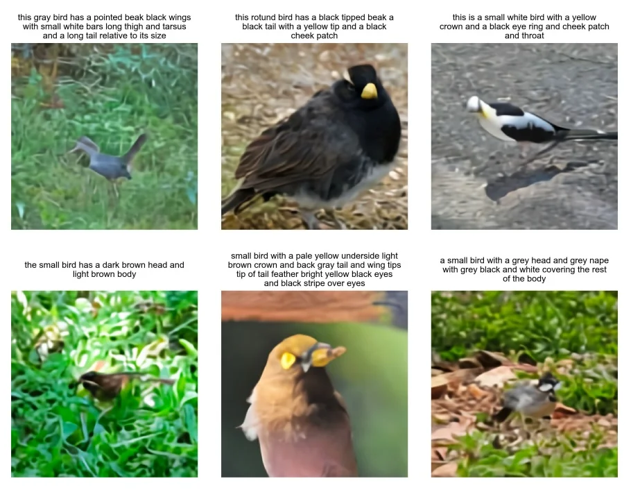
To address these challenges, DALL\(\cdot \)E 1 employs a clever reranking mechanism using a pretrained contrastive image–text model (CLIP [512]). From a large pool of candidate generations sampled from the transformer, a subset is selected based on similarity to the input caption in CLIP’s joint embedding space. As shown in Figure 20.81, increasing the number of samples from which to rerank (e.g., from 64 to 512) yields clear improvements in FID and IS, showcasing the power of contrastive alignment as a decoding prior.
Despite its pioneering design, DALL\(\cdot \)E 1 reveals key bottlenecks that limit generation quality: a fixed-length symbolic latent space, limited spatial resolution, and reliance on an autoregressive transformer prone to compounding errors. Moreover, its VQ-VAE decoder constrains the expressiveness of fine details and textures, and contrastive reranking—while effective—adds inference-time complexity.
These limitations laid the foundation for a more powerful successor. DALL\(\cdot \)E 2 abandons discrete tokenization in favor of CLIP-guided diffusion priors and cascaded super-resolution modules, enabling photorealistic outputs, improved compositionality, and open-vocabulary generalization. The next section explores this evolution in depth.
Enrichment 20.11.3: DALL\(\cdot \)E 2: Diffusion Priors over CLIP Embeddings
System Overview and Architectural Shift DALL\(\cdot \)E 2 [524] departs from the discrete-token autoregressive modeling of its predecessor by adopting a continuous latent diffusion framework grounded in the semantics of natural language and vision. Instead of generating symbolic image tokens (as in VQ-VAE + Transformer), DALL\(\cdot \)E 2 generates continuous CLIP image embeddings and decodes them into pixels using diffusion. This shift introduces greater flexibility, semantic expressiveness, and compositional fluency.
The full text-to-image generation pipeline comprises three major components:
- A frozen CLIP model [512], which embeds both text and images into a shared latent space via contrastive learning. In this space, semantic similarity corresponds to vector proximity—images and captions referring to the same concept are mapped close together. However, CLIP is not generative: it provides a static embedding space but cannot sample new embeddings or synthesize images.
-
A diffusion prior, trained to generate a CLIP image embedding from a given text embedding. Although text and image embeddings coexist in the same CLIP space, they are not interchangeable. Text embeddings primarily encode abstract, high-level semantic intent—what the image should conceptually depict—while image embeddings capture concrete, fine-grained visual details necessary for rendering a realistic image. Critically, only a subset of the embedding space corresponds to actual, decodable images: this subset forms a complex manifold shaped by natural image statistics.
To bridge the gap between abstract language and rich visual detail, the diffusion prior learns to sample from the conditional distribution over image embeddings given a text embedding. Instead of performing a deterministic projection (which might land off-manifold), it gradually denoises a sample toward the manifold of valid image embeddings, guided by the semantic signal from the text. This process ensures that the generated embedding is:
- 1.
- Semantically aligned with the input caption—anchored by the shared CLIP space,
- 2.
- Plausibly decodable into a coherent, photorealistic image—i.e., close to regions populated by real image embeddings.
The diffusion formulation also allows for stochasticity, making it possible to draw diverse but valid image embeddings from the same text input—capturing the one-to-many relationship between language and vision. For instance, the caption “a cat on a windowsill” might yield images with different lighting, poses, styles, or backgrounds—all plausible and semantically correct, but visually distinct.
-
A diffusion decoder, trained to reconstruct a high-resolution image from a CLIP image embedding. This decoder is based on the GLIDE architecture and operates directly in pixel space, not in a learned latent space as in traditional latent diffusion models (LDMs). It synthesizes images via a denoising diffusion process that is conditioned on the sampled CLIP image embedding. To further enhance semantic fidelity, the decoder can also incorporate the original CLIP text embedding as auxiliary context, enabling techniques such as classifier-free guidance—where conditioning signals are dropped stochastically during training and later reintroduced at inference to steer generation more precisely.
To produce high-resolution images, DALL·E 2 employs a cascade of diffusion models: a base model first generates a low-resolution \( 64 \times 64 \) image, which is then successively refined by two separate diffusion upsamplers—each responsible for enhancing resolution (e.g., to \( 256 \times 256 \) and ultimately \( 1024 \times 1024 \)). This multi-stage pipeline allows coarse scene structure and global composition to be resolved early, with fine textures and details added progressively. The result is a photorealistic image that faithfully reflects the semantic intent of the input caption and preserves the structural coherence implied by the CLIP embedding.
This architecture separates high-level semantics from low-level synthesis: the CLIP text embedding anchors generation in linguistic meaning, while the diffusion prior produces a visually grounded CLIP image embedding that is both semantically aligned and statistically plausible. By modeling a distribution over such embeddings, the system captures the one-to-many nature of text-to-image mappings—allowing multiple visually distinct yet valid outputs for the same prompt. Importantly, it ensures that sampled image embeddings lie on the manifold of realistic images, enabling successful decoding by the diffusion decoder.
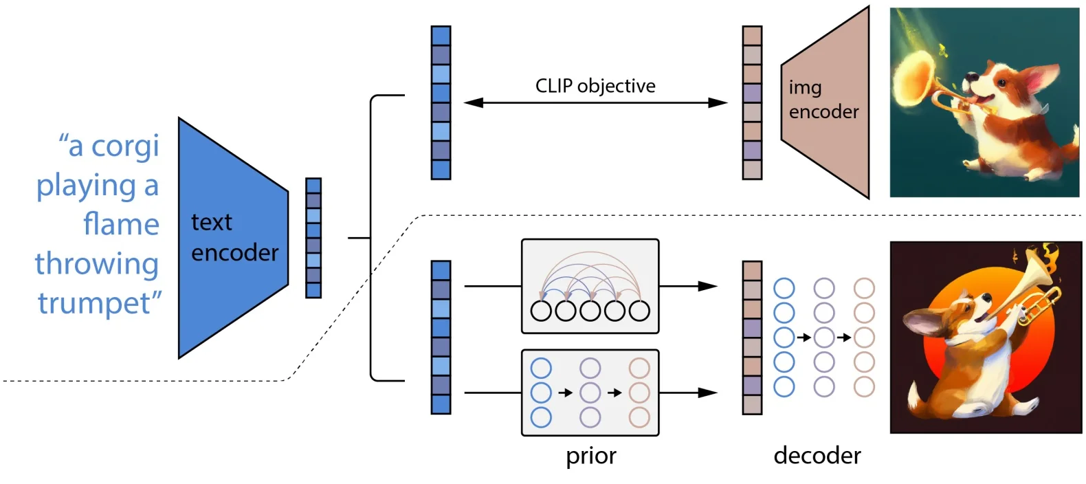
Diffusion Prior: Bridging Text and Image Embeddings The diffusion prior serves as a generative model that maps text embeddings to image embeddings—both produced by a frozen CLIP model [512]. This replaces the discrete-token autoregressive Transformer of DALL\(\cdot \)E 1 with a continuous, stochastic generative mechanism. Its primary role is to synthesize plausible image representations (in CLIP space) that semantically align with a given text prompt.
Training Objective The DALL\(\cdot \)E 2 prior models the conditional distribution \( p(z_i \mid z_t) \), where \( z_t \in \mathbb {R}^d \) is the CLIP text embedding derived from a caption \( y \), and \( z_i \in \mathbb {R}^d \) is the corresponding CLIP image embedding. This latent embedding \( z_i \) is not the image \( x \in \mathbb {R}^{H \times W \times 3} \), but a dense, semantic vector encoding the high-level content of the image. The role of the prior is to bridge language and vision by mapping \( z_t \) to a plausible, text-consistent image embedding \( z_i \).
As in standard DDPMs [232], a forward noising process progressively corrupts \( z_i \) over \( T \) timesteps: \[ z_i^{(t)} = \sqrt {\alpha _t} z_i + \sigma _t \boldsymbol {\epsilon }, \qquad \boldsymbol {\epsilon } \sim \mathcal {N}(0, \mathbf {I}), \] where \( z_i^{(t)} \) is the noisy latent at timestep \( t \), and the scalars \( \alpha _t, \sigma _t \) are defined by a cosine variance schedule [463]. The diffusion prior, modeled by a Transformer-based network \( f_\theta \), learns to recover \( z_i \) from \( z_i^{(t)} \), conditioned on \( z_t \) and timestep \( t \): \[ \mathcal {L}_{\mbox{prior}} = \mathbb {E}_{z_i, z_t, t} \left [ \left \| f_\theta (z_i^{(t)}, z_t, t) - z_i \right \|_2^2 \right ]. \]
Conditioning on text \( z_t \) and timestep \( t \): The diffusion prior \( f_\theta \) is a decoder-only Transformer that predicts the clean CLIP image embedding \( z_i \in \mathbb {R}^d \) from its noisy version \( z_i^{(t)} \), conditioned on the text prompt \( y \), the global CLIP text embedding \( z_t \in \mathbb {R}^d \), and the current diffusion timestep \( t \in \{1, \dots , T\} \). All components are embedded into a sequence of tokens, each of dimensionality \( d_{\mbox{model}} \), and processed jointly by the Transformer.
Input sequence construction: At every denoising step \( t \), the model receives a token sequence of length \( N + 2 \), where \( N \) is the number of caption sub-word tokens. The sequence is composed as follows:
- 1.
- CLIP text embedding token: The global CLIP text embedding \( z_t \in \mathbb {R}^{d_{\mbox{CLIP}}} \) is projected to the model’s internal dimension and prepended to the sequence.
- 2.
- Caption tokens: The raw text \( y \) is tokenized and embedded via a learned text encoder (separate from CLIP), yielding a sequence \( \texttt{Enc}(y) = [e_1, \dots , e_N] \in \mathbb {R}^{N \times d_{\mbox{model}}} \) that captures fine-grained linguistic details.
- 3.
- Noisy image token: The current noised image embedding \( z_i^{(t)} \in \mathbb {R}^{d_{\mbox{model}}} \) is appended as the final token in the sequence. This is both a conditioning signal and the slot from which the prediction is read.
A learned timestep embedding \( \gamma _t \in \mathbb {R}^{d_{\mbox{model}}} \) is added elementwise to each token in the sequence: \[ \texttt{Input}_t = \left [ \mbox{Proj}(z_t),\, e_1, \dots , e_N,\, z_i^{(t)} \right ] + \gamma _t + \mbox{PE}, \] where PE denotes positional embeddings. The Transformer attends over the entire sequence using standard self-attention layers.
Prediction mechanism: Unlike architectures that introduce a special [OUT] token, DALL\(\cdot \)E 2 reuses the position of the noisy image token to emit the prediction. That is, the model’s output at the final sequence position is interpreted as the predicted clean embedding: \[ \hat {z}_i = f_\theta (\texttt{Input}_t)_{N+2}. \] This vector is supervised using a mean squared error loss against the ground truth image embedding \( z_i \): \[ \mathcal {L}_{\mbox{prior}} = \mathbb {E}_{(z_i, z_t, y),\, t} \left [ \left \| \hat {z}_i - z_i \right \|_2^2 \right ]. \]
Intuition: This conditioning layout minimizes token overhead while enabling the model to integrate coarse semantic alignment (\( z_t \)), fine-grained linguistic context (\( \{e_k\} \)), temporal information (\( \gamma _t \)), and noisy visual evidence (\( z_i^{(t)} \)). By sharing the input and output slot for \( z_i^{(t)} \), the model tightly couples conditioning and generation, which empirically improves stability and sample quality in latent space. The model acts as a semantic denoiser, iteratively refining its belief over \( z_i \) in a manner consistent with both language and the manifold of realistic CLIP image embeddings.
Why predict \( z_i \) instead of noise \( \boldsymbol {\epsilon } \)? In standard DDPMs, models are often trained to predict the noise vector \( \boldsymbol {\epsilon } \) added to the data, rather than the clean data itself. However, DALL\(\cdot \)E 2 found that predicting the uncorrupted latent \( z_i \) directly yields better results in the CLIP space. This choice is empirically motivated.
Cosine Noise Schedule: The prior uses the improved cosine schedule [463], which spreads signal-to-noise ratio (SNR) more evenly across timesteps. This mitigates the sharp gradient imbalances found in linear schedules—where learning is dominated by either near-clean or near-noise states—and instead concentrates learning signal in mid-range latents, which are most ambiguous and informative.
Intuition: The prior functions as a semantic denoiser in CLIP space. At inference time, it starts from random Gaussian noise \( z_i^{(T)} \sim \mathcal {N}(0, \mathbf {I}) \), and iteratively transforms it into a coherent image embedding \( z_i^{(0)} \approx z_i \) via reverse diffusion steps. Each step is guided not by the noise offset, but by the model’s direct prediction of the destination \( z_i \), enabling more targeted and text-consistent updates. This ensures that the final image embedding is both decodable—i.e., maps to a natural image \( x \)—and semantically grounded in the input prompt \( y \).
Model Architecture Two alternative approaches were considered for modeling the conditional distribution \( p(z_i \mid z_t) \), where \( z_t \in \mathbb {R}^d \) is the CLIP text embedding of the caption \( y \), and \( z_i \in \mathbb {R}^d \) is the corresponding CLIP image embedding. Both approaches aim to generate latent image features aligned with the input caption, but differ substantially in modeling assumptions, architecture, and inference dynamics.
-
Transformer-based diffusion prior: This is the main method used in DALL\(\cdot \)E 2. It operates in latent space using a denoising diffusion process over CLIP image embeddings \( z_i \). At each timestep \( t \), the model is given a noisy latent \( z_i^{(t)} \), the global CLIP text embedding \( z_t \), and an embedded version of the timestep \( t \), and predicts the clean latent \( z_i \) directly.
Unlike UNet-based architectures used in pixel-space diffusion models such as DDPM [232] or GLIDE [464], the prior is implemented as a decoder-only Transformer. The inputs—caption tokens, CLIP embedding, timestep embedding, and noisy latent—form a compact sequence that is processed by self-attention layers, enabling flexible and global conditioning. This architecture naturally supports compositionality and long-range dependencies, which are more difficult to encode in convolutional models.
A key architectural departure from earlier DDPM-style models is the absence of pixel-level upsampling paths or spatial hierarchies; instead, the Transformer operates entirely in the flat CLIP embedding space. The model outputs the prediction from the same token slot that received the noisy image latent \( z_i^{(t)} \), avoiding the need for a dedicated output token and keeping conditioning tightly coupled with prediction.
- Autoregressive prior: As an alternative, the authors also experimented with an autoregressive model over compressed image embeddings. The embedding \( z_i \) is first reduced via PCA and quantized into a sequence of discrete tokens, which are then modeled using a Transformer decoder. This approach allows for non-iterative sampling, greatly reducing generation time. However, it was found to severely limit sample diversity and compositional robustness. It often failed to represent visually complex or semantically unusual prompts, such as “a snail made of harp strings,” and exhibited classic autoregressive weaknesses like mode collapse.
The diffusion-based prior was ultimately adopted due to its superior expressiveness, semantic grounding, and generalization capabilities. Its iterative nature enables it to sample from a rich, multimodal distribution over image embeddings—capturing the diversity of possible visual instantiations for a given text prompt. Importantly, this process ensures that sampled latents:
- Lie on the CLIP image manifold—i.e., they decode to realistic images.
- Align semantically with the caption embedding \( z_t \).
Comparison to previous diffusion works: The DALL\(\cdot \)E 2 prior shares conceptual lineage with diffusion models like “Diffusion Models Beat GANs” [123] and GLIDE [464], but with several notable distinctions:
- It operates entirely in a latent space (CLIP embeddings), rather than in pixel space.
- It uses a Transformer instead of a UNet, facilitating flexible conditioning on textual tokens and enabling better compositional generalization.
- The prediction target is the original embedding \( z_i \), not the noise \( \boldsymbol {\epsilon } \), a choice empirically found to improve convergence and alignment in semantic spaces.
Sampling efficiency: Although operating in CLIP latent space reduces the dimensionality of the generative process, diffusion models remain computationally intensive due to their iterative nature. Each sample requires \( T \) sequential denoising steps—commonly 1000 or more in traditional DDPMs [232]—which can severely limit inference speed.
To address this, DALL\(\cdot \)E 2 adopts the Analytic-DPM sampler [407], a high-order numerical solver designed to accelerate denoising without sacrificing quality. Unlike the original DDPM sampler, which performs fixed-step stochastic updates, Analytic-DPM approximates the reverse diffusion process as an ordinary differential equation (ODE) and solves it using techniques from numerical analysis. Specifically, it constructs closed-form approximations of the score function’s integral using high-order Runge–Kutta or multistep methods.
Intuition: Whereas classical DDPM sampling views denoising as a Markov chain with small, noisy steps, Analytic-DPM reinterprets it as a continuous trajectory through latent space and computes this path more efficiently. By leveraging smoothness in the learned score function and adapting step sizes accordingly, the sampler produces high-fidelity outputs using significantly fewer steps. In practice, this allows DALL\(\cdot \)E 2 to reduce sampling to just 64 steps—an order of magnitude faster than original DDPMs—while maintaining perceptual quality and semantic alignment.
Further acceleration is possible via progressive distillation [559], which trains a student model to mimic the multi-step sampling trajectory of a teacher using only a few steps. This method compresses multi-step DDIM-style inference into 4–8 steps, enabling near real-time generation without major loss in sample diversity or quality.
Future directions for improving the prior: DALL\(\cdot \)E 2’s latent diffusion prior leverages CLIP space to produce semantically aligned image embeddings. Still, there is room to improve its efficiency and controllability. One avenue is to enhance the text conditioning pathway, such as scaling the text encoder or introducing structured cross-attention. As shown in Imagen [557], boosting language understanding often yields greater perceptual gains than enlarging the generator.
In parallel, alternatives like Flow Matching [373] propose learning deterministic vector fields to transport samples from noise to target latents. Trained with optimal transport, this approach can shorten generative paths and accelerate sampling—making it a promising direction for future priors.
Together, these advances in conditioning and transport modeling inform newer architectures such as DALL\(\cdot \)E 3, which further optimize semantic grounding and inference speed.
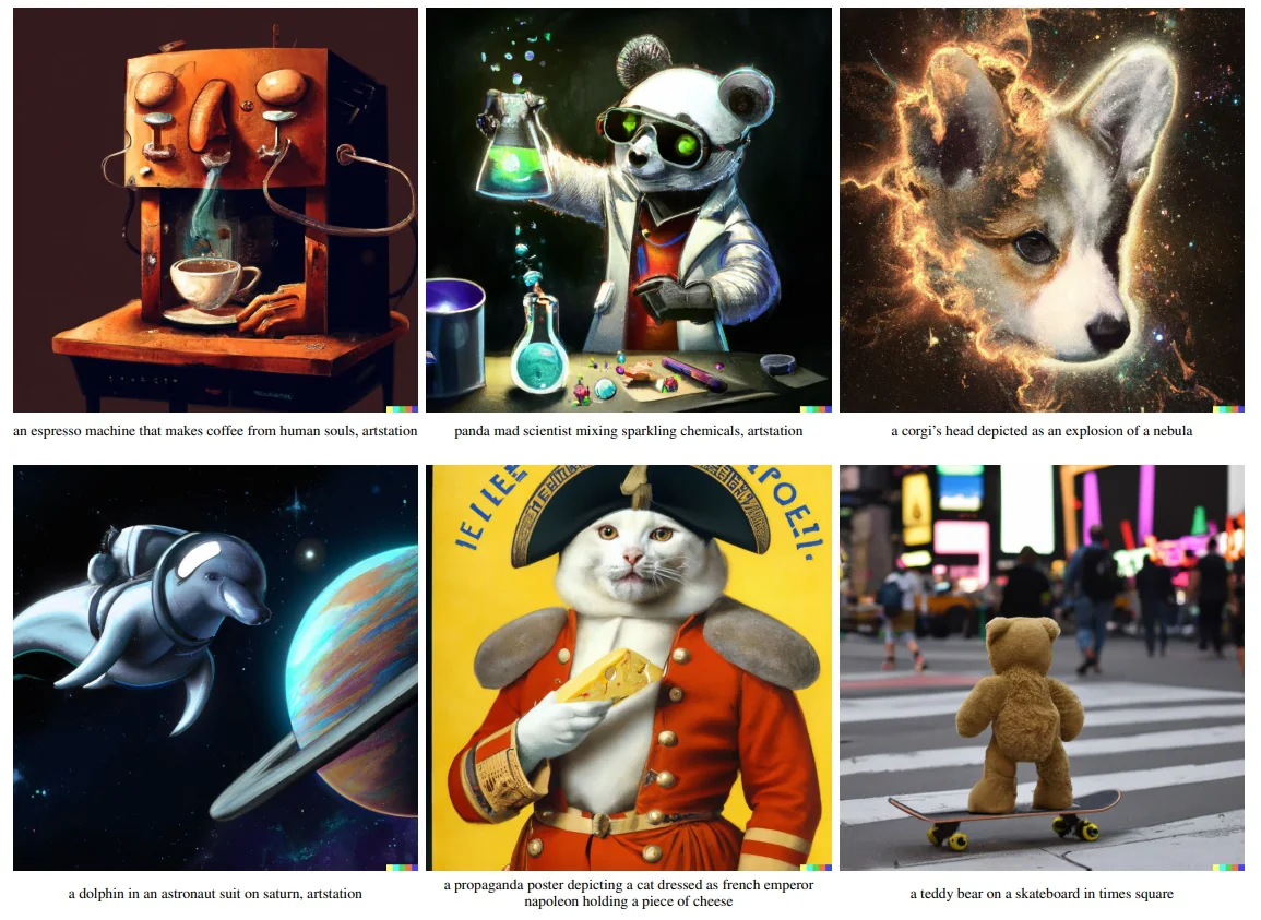
Diffusion-Based Decoder Once a CLIP image embedding \( \vec {z}_i \in \mathbb {R}^d \) is sampled from the diffusion prior, it is transformed into a photorealistic image by a cascade of diffusion models. This stage replaces the discrete VQ-VAE decoder used in DALL\(\cdot \)E 1 with a hierarchy of class-conditional diffusion models trained to generate increasingly detailed images from the continuous latent \( \vec {z}_i \). The decoder consists of three main components:
- A base decoder, trained to generate a \( 64 \times 64 \) RGB image from Gaussian noise conditioned on \( \vec {z}_i \).
- A mid-level super-resolution model, which upsamples the \( 64 \times 64 \) output to \( 256 \times 256 \), conditioned on both \( \vec {z}_i \) and the lower-resolution image.
- A high-resolution super-resolution model, which refines the image from \( 256 \times 256 \) to \( 1024 \times 1024 \), again conditioned on both \( \vec {z}_i \) and the previous output.
Each module in the cascade is implemented as a U-Net [549], modified to support semantic conditioning via cross-attention. At multiple layers within the U-Net, the CLIP image embedding \( \vec {z}_i \in \mathbb {R}^d \) is first projected through a learned MLP to produce a conditioning vector. This vector is then broadcast and used as the key and value in Transformer-style cross-attention blocks, where the U-Net’s intermediate activations serve as queries. This mechanism enables the model to inject global semantic context into spatially localized features during each denoising step.
This architecture follows the conditional pathway introduced in GLIDE (see Enrichment Enrichment 20.10.4), where cross-attention is used to integrate text embeddings. However, DALL\(\cdot \)E 2 replaces textual input with the CLIP image embedding \( \vec {z}_i \), and applies this conditioning across a cascade of three independently trained diffusion models—each specialized for a different output resolution.
All diffusion modules are trained separately using the standard noise prediction objective from denoising diffusion probabilistic models (DDPMs). Given a clean training image \( \vec {x}_0 \sim p_{\mbox{data}} \), the forward process produces noisy versions \( \vec {x}_t \) at discrete timesteps \( t \in \{1, \dots , T\} \) using the variance-preserving formulation: \[ \vec {x}_t = \sqrt {\bar {\alpha }_t} \vec {x}_0 + \sqrt {1 - \bar {\alpha }_t} \boldsymbol {\epsilon }, \quad \boldsymbol {\epsilon } \sim \mathcal {N}(0, I), \] where \( \bar {\alpha }_t \) defines a precomputed noise schedule. Each model is trained to predict \( \boldsymbol {\epsilon } \) from \( \vec {x}_t \), conditioned on both \( t \) and the CLIP embedding \( \vec {z}_i \), using the following loss: \[ \mathcal {L}_{\mbox{decoder}} = \mathbb {E}_{\vec {x}_0, \vec {z}_i, t, \boldsymbol {\epsilon }} \left [ \lambda (t) \cdot \left \| \boldsymbol {\epsilon } - \boldsymbol {\epsilon }_\theta (\vec {x}_t, t, \vec {z}_i) \right \|_2^2 \right ], \] where \( \lambda (t) \) is a weighting function that emphasizes earlier timesteps, which are often more uncertain and semantically significant.
Each model in the cascade integrates the global semantic embedding \( \vec {z}_i \) using cross-attention blocks inserted at multiple resolutions within a U-Net backbone. This mechanism allows the decoder to preserve semantic alignment throughout the generation process—from coarse layout at \( 64 \times 64 \) to fine-grained detail at \( 1024 \times 1024 \).
To upscale intermediate outputs, each super-resolution model is conditioned on both the CLIP embedding \( \vec {z}_i \) and the image produced by the preceding stage. These inputs are concatenated channel-wise and injected into the U-Net’s input layers, enabling the model to combine high-level semantics with spatial structure. This design preserves detail continuity across scales and mitigates the risk of semantic drift.
The cascaded diffusion strategy offers several advantages: modular training at different resolutions, efficient capacity allocation, and improved fidelity without sacrificing alignment. This architecture departs from the discrete token decoder used in DALL\(\cdot \)E 1, embracing a continuous latent refinement path. It also anticipates later systems such as Imagen [557] and Stable Diffusion [548], which similarly leverage latent diffusion and hierarchical super-resolution.
Semantic Interpolation and Reconstruction in CLIP Latents One of the key advantages of using CLIP image embeddings as the intermediate representation is the ability to manipulate and interpolate between visual concepts in a semantically meaningful way. Since the decoder learns to map from this continuous space to photorealistic images, it inherits the smoothness and structure of the CLIP embedding space.
DALL\(\cdot \)E 2 supports reconstruction from any CLIP image embedding \( \vec {z}_i \). This capability is demonstrated in reconstructions from progressively truncated principal components of the CLIP embedding. As shown in the following figure, low-dimensional reconstructions preserve coarse layout and object categories, while higher-dimensional reconstructions recover finer details such as texture, shape, and pose.
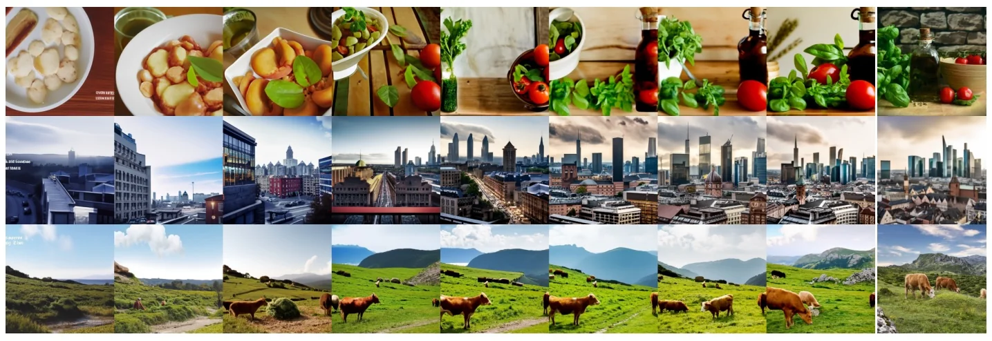
In addition, the model enables semantic variations by perturbing the CLIP embedding \( \vec {z}_i \) before decoding. By sampling different noise seeds or slightly shifting \( \vec {z}_i \), the decoder generates alternate renderings that retain the core semantics while altering attributes like style, viewpoint, or background content. This property is shown in the below figure, where variations of a logo and painting preserve their essential content while modifying incidental details.
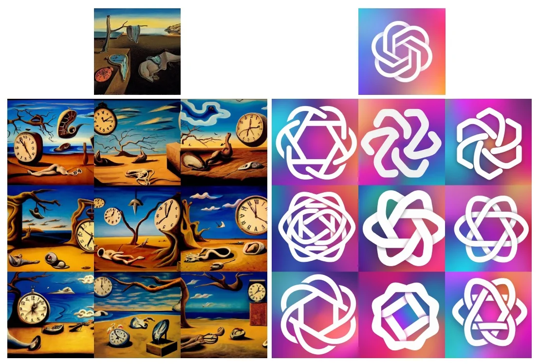
Beyond single-image variations, the decoder also supports interpolation between CLIP embeddings. Given two embeddings \( \vec {z}_i^{(1)} \) and \( \vec {z}_i^{(2)} \), one can linearly interpolate to create intermediate representations: \[ \vec {z}_i^{(\alpha )} = (1 - \alpha ) \cdot \vec {z}_i^{(1)} + \alpha \cdot \vec {z}_i^{(2)}, \quad \alpha \in [0, 1], \] and decode each \( \vec {z}_i^{(\alpha )} \) to obtain a smooth visual transition. The following figure illustrates this, showing how both content and style blend across the interpolation path.
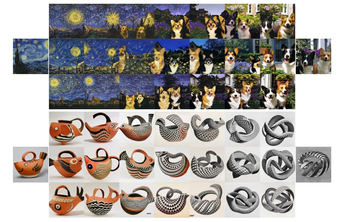
Further, textual edits can be translated into image modifications using vector arithmetic in CLIP space. If \( \vec {t}_1 \) and \( \vec {t}_2 \) are CLIP text embeddings corresponding to prompts like “a photo of a red car” and “a photo of a blue car”, one can construct: \[ \vec {z}_i^{\mbox{edited}} = \vec {z}_i + \lambda \cdot (\vec {t}_2 - \vec {t}_1), \] to steer the image generation toward a modified concept. This enables controlled, attribute-specific image edits as demonstrated in the below figure.
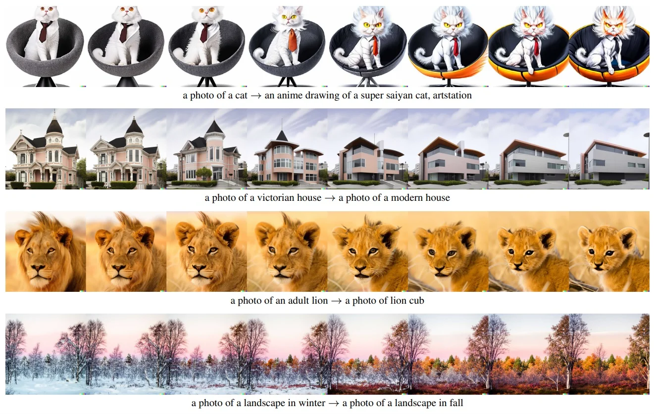
These capabilities demonstrate that the decoder does more than map a fixed vector to a fixed image—it enables meaningful navigation and manipulation within a high-dimensional semantic space. This design aligns well with human interpretability, creative applications, and interactive editing, bridging the gap between language and vision in a continuous and expressive manner.
Robustness and Generalization of the Decoder A notable strength of the DALL\(\cdot \)E 2 decoder lies in its ability to produce semantically coherent images even when faced with ambiguous or adversarial prompts. This property emerges from the decoder’s dependence on the CLIP image embedding \( \vec {z}_i \), which encodes high-level semantic content rather than raw text features. Despite the decoder’s lack of direct access to the original caption, its generation process remains surprisingly resilient.
The following figure exemplifies this phenomenon using typographic attacks. These are specially crafted images that contain misleading text elements designed to confuse vision-language models. The figure shows how, even when CLIP’s text-image alignment score is nearly zero for the correct label (e.g., “Granny Smith apple”), the decoder nonetheless produces plausible images consistent with the intended semantics.
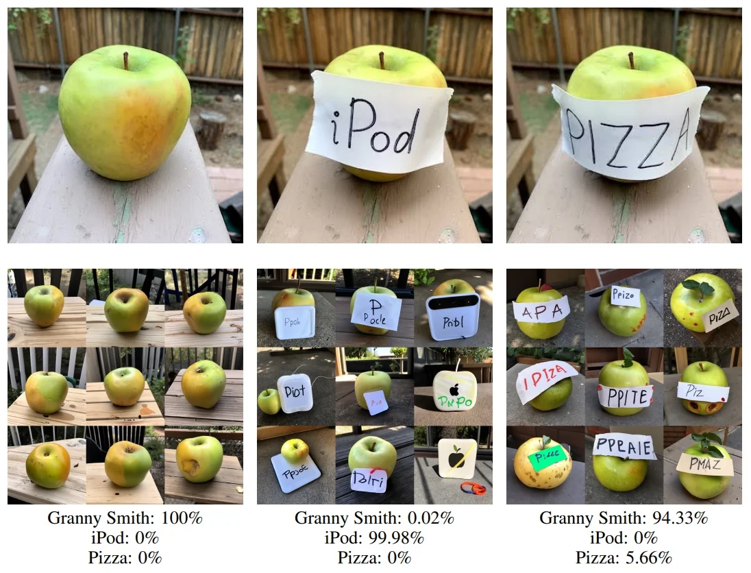
The decoder’s robustness stems partly from the structure of the CLIP latent space, which prioritizes high-level semantic attributes while discarding low-level noise [512]. By conditioning on global CLIP embeddings rather than raw pixels, the decoder inherits a degree of semantic abstraction and resilience. This acts as a form of latent filtering, enabling generalization across modest perturbations and preserving semantic coherence even under ambiguous or corrupted inputs.
However, the decoder also inherits CLIP’s limitations. Because CLIP is trained contrastively on noisy web-scale data, its latent space can reflect biases or fail in edge cases—such as typographic attacks [185] or adversarial prompts [820]. These vulnerabilities propagate directly into the decoder, which lacks any mechanism to question or correct the conditioning input. As a result, failures in CLIP—e.g., misinterpretation of text-image associations or overfitting to dominant visual styles—can manifest as incoherent or misleading generations.
These issues highlight the trade-offs of using frozen, independently trained encoders for generative tasks. While such encoders provide efficiency and stability, they limit adaptability: the decoder receives no gradient feedback about misaligned latents and cannot adjust its interpretation dynamically. Future directions may involve closer coupling between encoder and decoder—through joint training, adaptive conditioning, or feedback mechanisms—to improve robustness and mitigate failures under distributional shifts.
Dataset Construction and Semantic Pretraining The foundation of DALL\(\cdot \)E 2 lies in its use of the CLIP model [512], which defines a shared latent space for text and images. CLIP is pretrained on a massive, web-scale dataset comprising over 400 million image–caption pairs. This dataset—structurally similar to LAION [573]—is curated by crawling the internet for images with surrounding natural language descriptions, such as alt text or nearby HTML content.
Each image–text pair in the dataset is treated as a weakly supervised alignment between visual content and language. No manual annotation is performed; instead, the system relies on heuristics such as language filters, deduplication, and image-text consistency scores to ensure basic data quality. The resulting corpus exhibits high diversity in style, domain, and resolution, but also inherits noise, biases, and artifacts common to large-scale web data.
CLIP is trained using a symmetric contrastive loss (InfoNCE), in which paired text and image embeddings are pulled together in latent space, while unpaired examples are pushed apart. This strategy produces a semantic embedding space where proximity reflects conceptual similarity, enabling zero-shot recognition and flexible conditioning in downstream generative models.
Because DALL\(\cdot \)E 2 reuses this fixed latent space for both its prior and decoder, the properties of the CLIP dataset fundamentally shape the behavior of the generation pipeline. The abstract, high-level alignment captured by CLIP allows the model to generalize across prompts and visual styles—but also introduces inherited limitations, such as uneven category coverage, culturally specific associations, and susceptibility to adversarial captions [185, 820].
Future systems may benefit from cleaner or more targeted datasets, multi-modal filtering techniques, or joint training strategies that better align vision and language across diverse distributions. However, the scale and breadth of LAION-style corpora remain essential for achieving the wide generalization capabilities characteristic of models like DALL\(\cdot \)E 2.
Image Quality and Diversity: Qualitative and Quantitative Results DALL\(\cdot \)E 2 demonstrates a significant leap in both sample fidelity and diversity compared to earlier models such as DALL\(\cdot \)E 1 and GLIDE [464]. Its design leverages the semantic richness of the CLIP latent space and the spatial precision of cascaded diffusion decoders to generate high-resolution images that are both realistic and semantically aligned with input prompts.
To evaluate zero-shot generalization, the authors compare DALL\(\cdot \)E 2 with other models on MS-COCO prompts. As shown in the following figure, DALL\(\cdot \)E 2 consistently produces more photorealistic and diverse outputs, outperforming both DALL\(\cdot \)E 1 and GLIDE in terms of visual quality and semantic relevance.
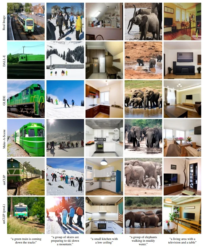
Qualitatively, the model captures fine stylistic variations and compositional semantics, even for abstract or imaginative prompts. Quantitatively, the authors report strong performance on both FID and CLIP score metrics, indicating a favorable balance between visual realism and prompt conditioning. Importantly, the model achieves these results without explicit caption-to-image pairing during decoder training, relying solely on alignment via CLIP embeddings.
Together, these findings affirm that at the time of publication, DALL\(\cdot \)E 2 achieved a new state-of-the-art in text-to-image synthesis, combining high sample quality with broad generalization and stylistic diversity.
Design Limitations and Architectural Tradeoffs Despite its impressive performance, DALL\(\cdot \)E 2 [524] exposes critical limitations that motivate further innovation. Most notably, the system’s reliance on a frozen CLIP encoder [512] introduces a structural bottleneck: the decoder generates images not from text directly, but from a static image embedding \( \vec {z}_i \) inferred from the CLIP text embedding \( \vec {z}_t \). This detachment limits the model’s capacity to resolve ambiguities in prompts or adapt to subtle shifts in meaning, especially for underrepresented concepts.
Because CLIP is pretrained independently on noisy web-scale data, it inherits biases and semantic gaps that the decoder cannot overcome. This can lead to mismatches between the user’s intention and the generated image, particularly in edge cases or when precision is required. Moreover, the three-stage pipeline—comprising the frozen encoder, the diffusion prior, and the cascaded decoder—adds system complexity and introduces potential fragility in the interfaces between components.
While this modular design supports reuse and targeted improvement, it also leads to a fragmented learning objective: no component is trained end-to-end with the final pixel output in mind. As a result, the system may excel in global compositionality but struggle with local consistency, prompting interest in more unified alternatives.
Stepping Towards Latent Diffusion Models The architecture of DALL\(\cdot \)E 2 [524] introduced a modular pipeline in which a frozen CLIP model provides a shared semantic space for both text and image, a diffusion prior generates image embeddings from text, and a cascaded decoder reconstructs full-resolution images. While this design offers flexibility and component reuse, it enforces strict boundaries between modules: the decoder receives only static CLIP embeddings, and the pipeline precludes gradient flow from image outputs back to the text encoder or semantic space. As a result, DALL\(\cdot \)E 2 cannot adapt its conditioning representations to improve prompt alignment or compositional accuracy during training. These limitations constrain its ability to generate coherent visual outputs for complex or nuanced captions.
Around the same time, Latent Diffusion Models (LDMs) [548] emerged as a unified alternative to modular architectures like DALL\(\cdot \)E 2. Instead of relying on frozen semantic embeddings as generation targets, LDMs train a variational autoencoder (VAE) to compress high-resolution images \( \vec {x} \in \mathbb {R}^{H \times W \times 3} \) into a spatially structured latent space \( \vec {z} \in \mathbb {R}^{h \times w \times d} \). This latent representation preserves both semantic content and spatial locality while significantly reducing dimensionality, allowing diffusion to operate over \( p(\vec {z}) \) rather than \( p(\vec {x}) \).
This decoupling of image space and generation space yields several key advantages. By performing diffusion in a compressed latent domain—typically of size \( h \times w \times d \) with \( h, w \ll H, W \)—LDMs significantly reduce the dimensionality of the generative process. This reduces memory consumption and accelerates training and inference, since the denoising network operates over fewer spatial locations and lower-resolution feature maps. While the final output must still be decoded into a full-resolution image, working in latent space greatly reduces the number of operations performed during iterative sampling.
Equally important is the spatial structure of the latent representation. Unlike global vectors such as CLIP embeddings—which collapse all spatial variation into a single descriptor—LDMs retain two-dimensional topology in the latent tensor \( \vec {z} \in \mathbb {R}^{h \times w \times d} \). This means that different spatial positions in \( \vec {z} \) can correspond to different image regions, allowing localized control and making it possible to model object layout, interactions, and spatial dependencies directly within the generative process.
Conditioning in LDMs is typically handled by a frozen text encoder (e.g., CLIP or T5), but rather than being used as a generation target, its features are injected into the denoising U-Net via transformer-style cross-attention modules at multiple spatial resolutions. This allows the model to integrate textual guidance at each step of the generation process.
This architectural strategy yields several compositional advantages:
- Spatially grounded text control: Prompt components (e.g., “a red ball on the left, a blue cube on the right”) can influence corresponding spatial locations in \( \vec {z} \), allowing for position-aware generation.
- Support for complex scene structure: The model can synthesize multiple entities with varied poses, attributes, and spatial relationships, reflecting the structure and grammar of the input prompt.
- Incremental and localized alignment: Because conditioning is applied repeatedly throughout the U-Net, the model can iteratively refine alignment with the prompt during denoising—rather than relying on a single global embedding passed at the start.
While the VAE and diffusion model are commonly trained separately for modularity and ease of optimization, they can also be fine-tuned jointly. This allows the learned latent space to adapt more directly to the generation task, potentially improving sample coherence and prompt fidelity.
In summary, LDMs replace static, globally pooled embeddings with a spatially structured, semantically responsive framework—laying the foundation for a new generation of controllable and scalable generative models. Although not originally proposed as a corrective to DALL\(\cdot \)E 2, LDMs address many of its limitations, such as the reliance on fixed embeddings, lack of spatial awareness, and modular non-differentiability. Stable Diffusion, released in mid-2022, embodies this design philosophy, offering high-resolution, prompt-aligned generation through a fully open and extensible latent diffusion pipeline.
OpenAI’s DALL\(\cdot \)E 3, introduced subsequently, is widely believed to adopt similar principles—including latent diffusion and closer integration with large language models such as GPT-4—to improve prompt adherence and editing flexibility. However, due to the proprietary nature of its architecture and training methodology, we now focus on the open and reproducible advances of latent diffusion models, which provide a transparent and theoretically grounded foundation for modern text-to-image generation.
Enrichment 20.11.4: Latent Diffusion Models (LDMs)
Overview and Conceptual Shift Latent Diffusion Models (LDMs) [548] represent a key evolution in generative modeling by addressing the inefficiencies of pixel-space diffusion. Traditional diffusion models, while powerful, operate directly over high-dimensional image tensors \( \vec {x} \in \mathbb {R}^{H \times W \times 3} \), making both training and sampling computationally expensive—especially for high-resolution generation. LDMs resolve this by first learning a perceptual autoencoder that maps images to a compact, spatially-structured latent space \( \vec {z} \in \mathcal {Z} \). Instead of modeling raw pixels, the denoising diffusion process unfolds within this learned latent space, where semantics are preserved but uninformative low-level details are abstracted away.
This architectural shift yields several benefits. Operating in \( \mathcal {Z} \) drastically reduces memory and compute costs, enabling high-resolution synthesis on modest hardware. The latent space is trained to preserve visually meaningful structures, improving the efficiency of generation. Moreover, conditioning signals—such as text, class labels, or image layouts—can be integrated directly into the latent denoising process via cross-attention mechanisms, giving rise to controllable, modular, and semantically aligned generation. We begin by braking down the components and training stages of LDMs, highlighting their conceptual differences from earlier approaches like DALL\(\cdot \)E 2 and motivating their widespread adoption in modern generative pipelines.
Autoencoder Architecture and Training Objective Latent Diffusion Models (LDMs) [548] begin by compressing images into a spatially structured latent space \( \vec {z} \in \mathcal {Z} \subset \mathbb {R}^{H' \times W' \times C} \), where \( H', W' \ll H, W \). This compression is achieved using a continuous variational autoencoder (VAE), whose goal is to preserve semantic information while discarding perceptually redundant pixel-level detail. The resulting latent representation balances fidelity with efficiency, enabling tractable diffusion modeling at high resolutions.
The encoder \( \mathcal {E}_\phi \) consists of a deep convolutional residual network that progressively downsamples the input image and outputs per-location Gaussian parameters \( (\boldsymbol {\mu }, \log \boldsymbol {\sigma }^2) \). Latent codes are sampled using the reparameterization trick: \[ \vec {z} = \boldsymbol {\mu }(x) + \boldsymbol {\sigma }(x) \odot \boldsymbol {\epsilon }, \qquad \boldsymbol {\epsilon } \sim \mathcal {N}(0, \mathbf {I}), \] ensuring differentiability for stochastic latent sampling. The decoder \( \mathcal {D}_\theta \) mirrors this structure with transposed convolutions and residual upsampling blocks to reconstruct the image \( \hat {x} = \mathcal {D}_\theta (\vec {z}) \).
The training objective combines four complementary losses:
- Pixel-level reconstruction loss: Ensures basic structural and color fidelity between the input and reconstruction. Typically chosen as \( \ell _1 \) or \( \ell _2 \) loss: \[ \mathcal {L}_{\mbox{pixel}} = \| x - \hat {x} \|_1 \quad \mbox{or} \quad \| x - \hat {x} \|_2^2. \] While effective at preserving coarse structure, this term alone often leads to overly smooth or blurry outputs due to averaging across plausible reconstructions.
- Perceptual loss (LPIPS): Mitigates blurriness by comparing activations (extraxcted features) from a pretrained CNN acting as a feature extractor \( \phi \), such as VGG16, in its final layer or in multiple intermediate layers: \[ \mathcal {L}_{\mbox{percep}} = \| \phi (x) - \phi (\hat {x}) \|_2^2. \] This loss encourages the decoder to preserve semantic and texture-level features, such as object boundaries and surface consistency, beyond raw pixels.
- KL divergence: Encourages the encoder’s approximate posterior \( q(\vec {z} \mid \vec {x}) \) to remain close to a fixed Gaussian prior \( \mathcal {N}(0, \mathbf {I}) \), \[ \mathcal {L}_{\mbox{KL}} = D_{\mbox{KL}} \left ( q(\vec {z} \mid \vec {x}) \parallel \mathcal {N}(0, \mathbf {I}) \right ). \] This term imposes structure and compactness on the latent space \( \mathcal {Z} \), which is essential for stable sampling and meaningful interpolation. By aligning \( q(\vec {z} \mid \vec {x}) \) with an isotropic Gaussian, the model ensures that randomly sampled latents resemble those seen during training—preventing degenerate or out-of-distribution samples. Moreover, it facilitates smoother transitions across the latent manifold, which is critical for tasks like class interpolation, latent editing, and controllable generation.
- Adversarial loss (optional): Introduced to restore high-frequency details that perceptual losses may not fully capture. A PatchGAN-style discriminator \( D \) is trained to distinguish real versus reconstructed patches: \[ \mathcal {L}_D = -\log D(x) - \log (1 - D(\hat {x})), \qquad \mathcal {L}_{\mbox{adv}} = -\log D(\hat {x}). \] This setup improves realism by aligning reconstructions with the local statistics of natural images, especially for textures such as hair, fabric, and foliage.
The total loss combines these components with tunable weights: \[ \mathcal {L}_{\mbox{total}} = \lambda _1 \mathcal {L}_{\mbox{pixel}} + \lambda _2 \mathcal {L}_{\mbox{percep}} + \lambda _3 \mathcal {L}_{\mbox{KL}} + \lambda _4 \mathcal {L}_{\mbox{adv}}. \]
In contrast to VQ-VAE architectures that discretize latents using a finite codebook, LDMs adopt a continuous latent space, allowing gradients to flow smoothly through the encoder and decoder. This continuity facilitates stable optimization. Furthermore, unlike approaches such as DALL\(\cdot \)E 2 that rely on frozen, externally trained embeddings (e.g., CLIP), the latent space \( \mathcal {Z} \) in LDMs is learned directly from data and refined through perceptual and adversarial objectives. As a result, the representations are not only compact but also well-aligned with the generative process, improving synthesis quality and of greater adaptability to the training domain.
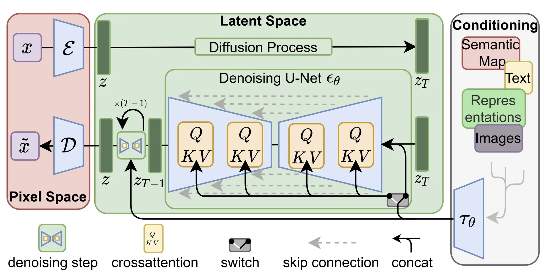
Autoencoder Architecture and Latent Normalization Latent Diffusion Models (LDMs) [548] begin by compressing high-resolution images \( x \in \mathbb {R}^{H \times W \times 3} \) into a spatially structured latent representation \( \vec {z} \in \mathbb {R}^{h \times w \times C} \), where \( h \ll H \), \( w \ll W \), and typically \( C = 4 \). This compression is performed by a perceptual autoencoder consisting of a convolutional encoder \( \mathcal {E}_\phi \) and decoder \( \mathcal {D}_\theta \), trained separately from the generative diffusion model.
Encoder and Decoder Design The encoder \( \mathcal {E}_\phi \) is built from residual convolutional blocks with stride-2 downsampling, group normalization, and a spatial self-attention layer near the bottleneck. Rather than directly outputting the latent \( \vec {z} \), the encoder predicts a distribution over latents by producing two tensors of shape \( \mathbb {R}^{h \times w \times C} \): the mean \( \boldsymbol {\mu } \) and the log-variance \( \log \boldsymbol {\sigma }^2 \). These are concatenated into a single tensor of shape \( \mathbb {R}^{h \times w \times 2C} \) and used to sample latents via the reparameterization trick:
\[ \vec {z} = \boldsymbol {\mu } + \boldsymbol {\sigma } \odot \boldsymbol {\epsilon }, \qquad \boldsymbol {\epsilon } \sim \mathcal {N}(0, \mathbf {I}). \]
The decoder \( \mathcal {D}_\theta \) mirrors the encoder’s structure using upsampling residual blocks and convolutions. The final output passes through a tanh activation to restrict pixel values to the range \( [-1, 1] \), ensuring alignment with the normalized image input domain and promoting numerical stability.
# From ldm/modules/autoencoder/modules.py

class AutoencoderKL(nn.Module):
    def encode(self, x):
        h = self.encoder(x)              # Conv + ResBlock + Attention
        moments = self.quant_conv(h)     # Projects to (mu, logvar)
        return moments

    def decode(self, z):
        z = self.post_quant_conv(z)      # Linear 1x1 conv
        x_hat = self.decoder(z)          # Upsample + Conv stack
        return torch.tanh(x_hat)         # Outputs in [-1, 1]
Latent Normalization for Diffusion Compatibility After training the autoencoder, the encoder \( \mathcal {E}_\phi \) maps images \( x \in \mathbb {R}^{H \times W \times 3} \) to continuous latent representations \( \vec {z} \in \mathbb {R}^{h \times w \times C} \) via reparameterized sampling. These latents, however, typically have a standard deviation significantly larger than 1 (e.g., \( \hat {\sigma }_{\vec {z}} \approx 5.49 \) on ImageNet \( 256 \times 256 \)), since the encoder has not been trained with any constraint to normalize the latent scale.
To ensure compatibility with the noise schedules and assumptions of the downstream diffusion model—specifically, that the initial inputs should lie within a distribution close to \( \mathcal {N}(0, \mathbf {I}) \)—the latents are globally normalized by a scalar factor \( \gamma \), defined as the reciprocal of their empirical standard deviation:
\[ \tilde {\vec {z}} = \gamma \cdot \vec {z}, \qquad \gamma = \frac {1}{\hat {\sigma }_{\vec {z}}}. \]
This normalization is applied after training the autoencoder but before training the diffusion model. It ensures that the scale of the latent representations matches the variance assumptions of the DDPM forward process, allowing the use of standard Gaussian-based noise schedules (e.g., cosine or linear beta schedules) without requiring architectural or hyperparameter adjustments.
For example, if the empirical standard deviation of \( \vec {z} \) is \( \hat {\sigma }_{\vec {z}} = 5.49 \), then \( \gamma \approx 0.18215 \). This calibrated latent distribution becomes the new data domain \( \mathcal {Z} \subset \mathbb {R}^{h \times w \times C} \) over which the denoising diffusion model is trained.
By aligning the latent distribution with the assumptions of the diffusion framework, this scaling step improves training stability and sample quality, while retaining the benefits of working in a compact and perceptually aligned representation space.
Denoising Diffusion in Latent Space Once the variational autoencoder has been trained and frozen, Latent Diffusion Models (LDMs) reformulate the generative process as a denoising task in the latent space \( \mathcal {Z} \subset \mathbb {R}^{h \times w \times C} \). Rather than modeling high-dimensional pixel distributions, a Denoising Diffusion Probabilistic Model (DDPM) [232] is trained to model the distribution of latents produced by the encoder \( \mathcal {E}_\phi (x) \). For background on diffusion model fundamentals, see 20.9.0.1.0.
Given a clean latent \( z_0 = \mathcal {E}_\phi (x) \), the forward process gradually corrupts it through a fixed Markov chain: \[ q(z_t \mid z_{t-1}) = \mathcal {N}(z_t ; \sqrt {1 - \beta _t} \, z_{t-1}, \beta _t \, \mathbf {I}), \qquad q(z_t \mid z_0) = \mathcal {N}\left (z_t ; \sqrt {\bar {\alpha }_t} \, z_0, (1 - \bar {\alpha }_t) \, \mathbf {I} \right ), \] where \( \bar {\alpha }_t = \prod _{s=1}^t (1 - \beta _s) \) accumulates the noise schedule.
The denoising network \( \epsilon _\theta \) is trained to predict the noise \( \epsilon \sim \mathcal {N}(0, \mathbf {I}) \) added to the latent at each step. The objective is a mean-squared error loss: \[ \mathcal {L}_{\mbox{denoise}} = \mathbb {E}_{z_0, \epsilon , t} \left [ \left \| \epsilon - \epsilon _\theta (z_t, t, \tau ) \right \|_2^2 \right ], \] where \( z_t = \sqrt {\bar {\alpha }_t} \, z_0 + \sqrt {1 - \bar {\alpha }_t} \, \epsilon \), and \( \tau \in \mathbb {R}^{N \times d} \) is a sequence of embedded caption tokens from a frozen CLIP text encoder.
Importantly, all operations take place in the compressed latent space. The output \( z_0 \) of the reverse diffusion process is never directly decoded from the text, but instead synthesized through iterative noise removal guided by linguistic context. Only after this denoised latent is produced does the VAE decoder \( \mathcal {D}_\theta \) reconstruct the final image—bridging the semantic alignment in latent space with rendering in pixel space.
We now examine the architecture of \( \epsilon _\theta \), which must reconcile temporal, spatial, and textual conditioning across the entire denoising trajectory.
Architecture of the Denoising U-Net In Latent Diffusion Models (LDMs) [548], the denoising network \( \epsilon _\theta \) is a modified U-Net that operates entirely within a learned latent space \( \vec {z}_t \in \mathbb {R}^{h \times w \times C} \), where spatial structure is preserved despite dimensionality reduction. This latent space is produced by a pre-trained VAE encoder \( \mathcal {E}_\phi \), which maps high-resolution images \( x \in \mathbb {R}^{H \times W \times 3} \) into compact latent representations. During inference, the VAE decoder \( \mathcal {D}_\theta \) reconstructs the final image from a denoised latent \( \vec {z}_0 \). Thus, generation is fully decoupled from rendering: the diffusion model performs structured denoising in latent space, and the VAE handles the final image synthesis.
- Residual blocks: Each resolution stage of the U-Net uses residual blocks composed of convolution, group normalization, and nonlinearity, with a skip path that adds the block’s input to its output. This improves gradient flow and stability across the network depth, while supporting effective feature reuse in the latent space.
- Skip connections: Encoder–decoder symmetry is preserved by lateral skip connections that pass early, high-resolution latent features to later decoding stages. These connections maintain fine-grained spatial information—such as object boundaries and texture—that may otherwise degrade through diffusion noise and downsampling.
- Self-attention layers: Near the bottleneck, self-attention modules allow each latent location to attend to the full latent map. This models long-range dependencies critical for spatial relations like “above,” “behind,” or “next to,” and enables coherent global structure during denoising.
- Timestep conditioning: At each denoising step \( t \), the model is informed of the expected noise level via sinusoidal embeddings \( \vec {e}_t \), projected through an MLP to a vector \( \vec {\gamma }_t \in \mathbb {R}^C \). This conditioning vector is broadcast and added to intermediate feature maps \( \vec {h} \in \mathbb {R}^{C \times h \times w} \) inside each residual block: \[ \vec {h}' = \vec {h} + \mbox{Proj}(\vec {\gamma }_t). \] This simple additive modulation allows the model to adapt its behavior across timesteps, progressively refining coarse structure into fine detail as \( t \to 0 \).
-
Cross-attention conditioning: Semantic control is introduced via transformer-style cross-attention blocks applied at multiple U-Net resolutions. Given a caption embedding \( \tau \in \mathbb {R}^{N \times d} \), obtained from a frozen CLIP text encoder, each spatial feature in the latent map \( \vec {z}_t \in \mathbb {R}^{h \times w \times C} \) is projected to a query vector. The tokens in \( \tau \) are projected into keys and values. Attention is computed as: \[ \mbox{Attention}(\vec {q}, \vec {K}, \vec {V}) = \mbox{softmax}\left (\frac {\vec {q} \cdot \vec {K}^\top }{\sqrt {d}}\right )\vec {V}. \] This enables each latent location to dynamically attend to the most relevant parts of the prompt. For instance, if the caption is “a red cube on the left and a blue sphere on the right,” left-side latents focus more on “red cube,” while right-side latents emphasize “blue sphere”.
The advantages of this formulation include:
- Spatial specificity: Token-level attention guides individual regions of the latent map, enabling localized control.
- Semantic compositionality: Different parts of the prompt influence different subregions of the latent, enabling compositional generation.
- Dynamic guidance: The prompt influences the denoising at every step, enabling consistent semantic alignment throughout the trajectory.
This contrasts with global CLIP embedding approaches used in DALL\(\cdot \)E 2, which apply the prompt as a static conditioning vector, losing fine spatial control. Here, cross-attention integrates linguistic semantics into spatial generation at every scale and timestep.
Note on latent–image alignment: One might worry that the denoised latent \( \vec {z}_0 \) produced by the diffusion model may not match the distribution of latents seen by the VAE decoder during training. However, the diffusion model is explicitly trained to reverse noise from latents \( \vec {z}_0 \sim \mathcal {E}_\phi (x) \). Its denoised outputs are thus learned to lie within the latent manifold that the decoder \( \mathcal {D}_\theta \) can reconstruct from. The VAE does not condition on the text; instead, semantic alignment is handled entirely in the latent space through cross-attention before decoding. This separation ensures high-quality, efficient, and semantically grounded image generation.
Enrichment 20.11.4.1: Decoder Fidelity Without Explicit Text Conditioning
A natural concern in Latent Diffusion Models (LDMs) [548] is that the VAE decoder \( \mathcal {D}_\theta \) is not conditioned on the caption at inference. The diffusion model generates a latent code \( \vec {z}_0 \in \mathcal {Z} \) based on text input, but the decoder reconstructs an image from \( \vec {z}_0 \) unconditionally. This raises the question:
Can prompt-specific details be lost if the decoder never sees the text?
Why It Still Works Although the decoder ignores the caption, it operates on latents that were explicitly shaped by a text-conditioned diffusion model. The prompt’s semantics—object types, positions, colors—are baked into \( \vec {z}_0 \). The decoder’s job is not to reason about the prompt, but to faithfully render its visual realization from the latent code.
This works because:
- The VAE is trained to reconstruct real images from latents produced by its encoder, ensuring good coverage over \( \mathcal {Z} \).
- The compression factor (e.g., 4x or 8x) is modest, preserving fine detail.
- The diffusion model is trained on the encoder’s latent distribution, so its outputs lie within the decoder’s domain.
Trade-offs and Alternatives While this design is efficient and modular, it assumes the latent code captures all prompt-relevant detail. This may falter with subtle prompts (e.g., “a sad astronaut” vs. “a smiling astronaut”) if distinctions are too fine for \( \vec {z}_0 \) to preserve.
To address this, other models extend conditioning beyond the latent stage:
- DALL\(\cdot \)E 2 (unCLIP) [524] uses a second-stage decoder conditioned on CLIP embeddings.
- GLIDE and Imagen apply prompt conditioning throughout a cascaded diffusion decoder.
These improve prompt alignment, especially for fine-grained attributes, but increase compute cost and architectural complexity.
Conclusion In LDMs, text guidance occurs entirely in latent space—but that’s usually sufficient: if the denoised latent \( \vec {z}_0 \) accurately reflects the caption, the decoder can render it without ever “reading” the prompt. While newer models extend semantic control to the pixel level, LDMs offer an elegant and effective trade-off between simplicity and fidelity.
Classifier-Free Guidance (CFG) To enhance semantic alignment during sampling, Latent Diffusion Models incorporate Classifier-Free Guidance (CFG) [233]. Rather than relying on external classifiers to guide generation, the model is trained with randomly dropped conditioning information, enabling it to interpolate between conditional and unconditional outputs at inference time. The final prediction is given by:
\[ \hat {\boldsymbol {\epsilon }}_{\mbox{CFG}} = (1 + \lambda ) \cdot \hat {\boldsymbol {\epsilon }}_\theta (\vec {z}_t, t, \tau ) - \lambda \cdot \hat {\boldsymbol {\epsilon }}_\theta (\vec {z}_t, t, \varnothing ), \]
where \( \vec {z}_t \) is the latent at timestep \( t \), \( \tau \) is the CLIP-based text embedding, and \( \lambda \in \mathbb {R}_+ \) is a guidance weight. This simple yet powerful mechanism allows the diffusion process to be steered toward text-conformant latents while balancing visual diversity. For a detailed derivation and architectural breakdown, see Section Enrichment 20.9.3.
Empirical Results and Ablations LDMs have been evaluated across a wide range of tasks—unconditional generation, text-to-image synthesis, inpainting, and style transfer.
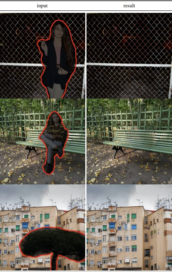
The authors conduct extensive ablations to identify design choices that contribute most to performance. Key insights include:
- Compression factor matters: Mild compression ratios (e.g., \( h, w \approx H/8, W/8 \)) retain sufficient perceptual detail for high-quality synthesis, outperforming VQ-based methods with more aggressive bottlenecks.
- Text-conditional cross-attention is essential: Removing spatial cross-attention layers results in poor prompt alignment, confirming that token-level attention is critical for semantic fidelity.
- Guidance scale tuning is nontrivial: Higher CFG values increase prompt adherence but reduce diversity and realism. For text-to-image synthesis, guidance scales in the range \( \lambda \in [4, 7] \) are often optimal.
- Decoder quality sets an upper bound: Even perfect latent alignment cannot recover prompt-relevant visual details if the decoder fails to reconstruct fine structure. Thus, VAE capacity indirectly limits generation fidelity.
- Task-specific fine-tuning improves quality: Inpainting, depth conditioning, and style transfer models trained on tailored objectives yield noticeably sharper and more controllable outputs than generic text-to-image models.
Limitations and Transition to Newer Works Like Imagen Latent Diffusion Models (LDMs) achieve a compelling trade-off between semantic guidance and computational efficiency by shifting diffusion to a compressed latent space. However, two key architectural limitations motivate newer designs:
- 1.
- Frozen CLIP Text Encoder: LDMs rely on a fixed CLIP encoder (e.g., ViT-B/32) for text conditioning, which was pretrained for contrastive image–text alignment, not generation. As such, it cannot adapt its embeddings to better serve the generative model. This limits the handling of nuanced prompts, rare entities, or abstract relationships, and its relatively small size constrains linguistic expressivity compared to large language models like T5-XXL.
- 2.
- Unconditional VAE Decoder: The decoder \( \mathcal {D}_\theta \) reconstructs images from latent vectors \( \vec {z}_0 \) without access to the guiding text prompt. While the denoising U-Net integrates semantic content into the latent, the decoder performs unconditional reconstruction. This design assumes the latent fully captures all prompt-relevant details—an assumption that may falter in complex or fine-grained prompts.
To address these issues, Imagen [557] introduces two key innovations:
- Richer Language Understanding: Instead of CLIP, Imagen uses a large frozen language model (T5-XXL) to encode prompts. This yields semantically richer and more flexible embeddings, better aligned with generation needs—even without end-to-end finetuning.
- Pixel-Space Diffusion: Imagen avoids latent compression during generation, performing denoising directly in pixel space or using minimal downsampling. This preserves visual detail and semantic fidelity more reliably than VAE-based reconstruction.
These improvements come at a cost: Imagen demands significantly higher computational resources during training and inference, due to both its larger backbone and pixel-level denoising. As explored next, the field continues to navigate the trade-off between efficiency and expressivity—balancing lightweight modularity with prompt-faithful generation quality.
Enrichment 20.11.5: Imagen: Scaling Language Fidelity in Text2Img Models
Motivation and Context Latent Diffusion Models (LDMs) [548] showed that pushing diffusion into a compressed VAE space slashes compute while preserving visual quality. Yet their design leaves all text conditioning to the UNet denoiser, because the VAE decoder itself is unconditional. For complex, compositional prompts, that separation can introduce subtle mismatches between what the caption asks for and what the pixels finally depict.
Imagen [557] turns this observation on its head. Through a careful ablation study the authors argue that text fidelity is limited more by the language encoder than by the image decoder. Scaling the caption encoder (T5 [517]) from Base to XXL delivers larger alignment gains than adding channels or layers to the diffusion UNets.
What is new in Imagen? The system freezes a 4.6-B-parameter T5-XXL to embed the prompt, then feeds that embedding into a three-stage diffusion cascade that progressively upsamples 64→256→1024 px. This coarse-to-fine recipe is familiar, but three engineering insights make Imagen unusually faithful to the text:
- Bigger language encoder \(>\) bigger image decoder. Ablations show that scaling the text backbone (e.g. T5-Large \(\rightarrow \) T5-XXL, \( \approx 4.6 \) B parameters) yields much larger improvements in prompt–image alignment than enlarging the diffusion UNets. Richer linguistic representations, not extra pixel capacity, are the main bottleneck.
- Dynamic-threshold CFG. Imagen applies classifier-free guidance but clips each predicted image to the adaptive \(p\)-th percentile before the next denoising step. This dynamic thresholding lets the sampler use higher guidance weights for sharper, more on-prompt images without colour wash-out or blown highlights.
- DrawBench. The authors curate a 200-prompt suite covering objects, spatial relations, counting, style, and abstract descriptions. In pairwise human studies on DrawBench, Imagen is preferred over both DALL·E 2 and Parti1.
In what follows we examine Imagen from four complementary angles:
- 1.
- Text \(\rightarrow \) Latent Coupling. We detail how the frozen T5-XXL encoder feeds its 4 096-dimensional embeddings into every UNet block, and why this cross-attention scheme is decisive for tight prompt grounding.
- 2.
- Three-Stage Diffusion Cascade. We walk through the \(64 \!\to \! 256 \!\to \! 1024\)-pixel pipeline and explain the dynamic-threshold variant of classifier-free guidance that stabilises high guidance weights without introducing blow-outs.
- 3.
- Ablation Take-aways. Side-by-side experiments reveal that scaling the language encoder delivers larger alignment gains than scaling the image UNets, and that guidance tuning outweighs most architectural tweaks.
- 4.
- Implications for Later Work. We point out how Imagen’s design choices foreshadow prompt-editing methods such as Prompt-to-Prompt and other text-controlled diffusion advances.
Cascaded Diffusion Pipeline
Imagen generates high-resolution images from text using a three-stage cascaded diffusion pipeline. A base model first synthesizes a coarse \( 64 \times 64 \) image conditioned on a text embedding. Two subsequent super-resolution (SR) diffusion models then refine this output to \( 256 \times 256 \) and finally to \( 1024 \times 1024 \), each conditioned on both the original text and the lower-resolution image. Noise conditioning augmentation is applied during SR training to improve robustness. This stage-wise design progressively enhances fidelity and detail while maintaining strong semantic alignment with the prompt.
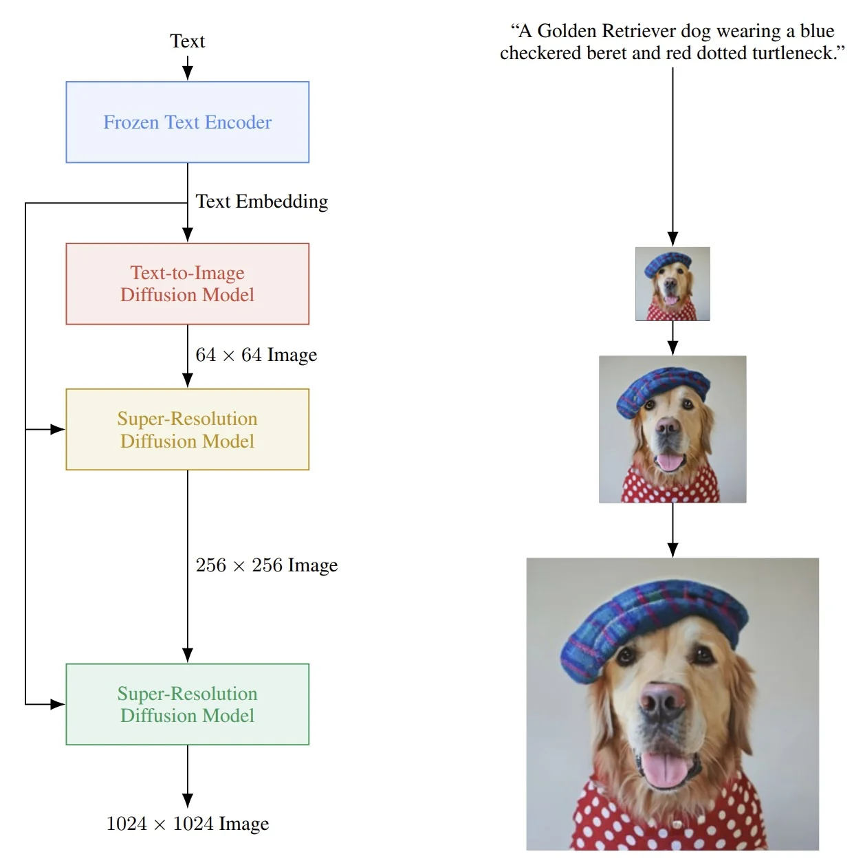
Classifier-Free Guidance and Dynamic Thresholding
As outlined in Section Enrichment 20.9.3, classifier-free guidance (CFG) improves text-image alignment by combining predictions from a conditional and an unconditional denoising model. In particular, given a noisy sample \( \vec {z}_t \) at timestep \( t \), the denoised prediction is adjusted as
\[ \hat {{x}}_0^{\,(\mbox{CFG})} = (1 + \lambda ) \, \hat {\epsilon }_\theta (\vec {z}_t, t, y) - \lambda \, \hat {\epsilon }_\theta (\vec {z}_t, t, \varnothing ), \]
where \( \lambda \geq 0 \) is the guidance weight. Larger \( \lambda \) values push samples closer to the conditional manifold, increasing semantic fidelity—but they also amplify sharp transitions, outliers, and pixel intensities. This may lead to unnatural results, especially in high-resolution stages like \( 1024 \times 1024 \).
Problem: Oversaturation from Large Guidance Without any correction, high CFG weights cause the predicted clean image \( \hat {{x}}_0 \) to exhibit pixel values far outside the dynamic range of natural images (e.g., \([-1, 1]\) in normalized space). This leads to:
- Oversaturated colors, especially in backgrounds or small object regions.
- Loss of contrast and detail due to hard clipping of extreme values.
- Reduced diversity across samples due to overly confident predictions.
Naïve Solution: Static Thresholding One straightforward way to ensure that the final image remains in the valid pixel range (e.g., \([-1, 1]\)) is to apply static thresholding—that is, clipping the predicted clean image \( \hat {x}_0 \) to lie within this range:
\[ \hat {x}_0^{\,(\mbox{clipped})} = \mbox{clip}(\hat {x}_0, -1, 1). \]
While simple, this solution can degrade image quality when applied at every denoising step. During the iterative reverse process, the model may temporarily predict pixel values outside the target range to represent subtle visual cues—such as specular highlights, sharp edges, or deep shadows. These out-of-range values often reflect meaningful structure that will eventually be pulled into range by the final denoising steps. If we aggressively clip at each step, we risk:
- Flattening high-contrast regions: Highlights or shadows may be prematurely truncated, reducing the image’s perceived depth and richness.
- Introducing artifacts: Hard cutoffs can produce unnatural boundaries or saturation plateaus, especially in smooth gradients or textured areas.
- Destroying predictive consistency: The model’s learned denoising trajectory may rely on temporarily overshooting the target range before converging. Clipping interferes with this path, leading to less coherent results.
Because of these issues, it is more effective to defer clipping until the final step of the denoising process—once \( \hat {x}_0 \) is fully predicted. However, even this final-step clipping can still be problematic if the distribution of predictions varies across samples. This limitation motivates more adaptive solutions such as dynamic thresholding, which adjusts the clipping range based on the specific prediction statistics of each sample.
Dynamic Thresholding: an Adaptive Alternative to Static Clipping Method. Dynamic thresholding [557] rescales each denoised prediction \( \hat {{x}}_0 \in \mathbb {R}^{H \times W \times 3} \) by a sample-specific scale before clipping to \([-1, 1]\). This scale \( s \) is set to the \( p \)-th percentile (typically \( p = 99.5 \)) of the absolute pixel magnitudes:
\[ s = \mbox{percentile}(|\hat {{x}}_0|,\; p), \quad \hat {{x}}_0^{\,(\mbox{dyn})} = \mbox{clip}\left ( \frac {\hat {{x}}_0}{s},\; -1,\, 1 \right ). \]
This adaptive rescaling ensures that only the top \( (100 - p)\% \) of pixel values—those with the most extreme magnitudes—are affected, while the bulk of the image retains its original brightness and contrast. By adapting the clipping threshold to each image individually, dynamic thresholding avoids global overcorrection and better preserves subtle visual detail.
Why it works (with examples and reasoning).
During denoising—especially under strong classifier-free guidance or at high resolutions—the model often predicts pixel values slightly outside the legal image range \([-1, 1]\). These excursions may encode meaningful high-frequency details (like glints, reflections, or fine textures), but they can also include spurious outliers (e.g., sharp halos, single-pixel spikes).
Static clipping flattens all values beyond this range, indiscriminately truncating both legitimate signal and noise. For example, if a predicted pixel value is \( \hat {x}_0 = 1.5 \) and the 99.5th percentile sets \( s = 1.4 \), then dynamic thresholding performs:
\[ \hat {x}_0 = 1.5 \longrightarrow \frac {1.5}{1.4} \approx 1.07 \longrightarrow \mbox{clipped to } 1.0, \quad \hat {x}_0 = 1.2 \longrightarrow \frac {1.2}{1.4} \approx 0.86 \quad \mbox{(preserved)}. \]
Here, even though both values exceed the legal range, only the more extreme outlier gets clipped. Crucially, rescaling does reduce the absolute intensity of all values, but it preserves their relative differences. The 1.2 pixel remains brighter than others around it, so its visual role as a highlight is maintained. This distinction would be erased by static clipping, which collapses all values above 1.0 into a hard ceiling.
Dynamic thresholding thus provides a soft-constraint mechanism that acts proportionally to the sample’s content:
- It preserves expressive range by maintaining contrast between midtones and peaks, avoiding the flattening effect of uniform truncation.
- It targets only extreme outliers—often isolated and perceptually disruptive—without globally lowering brightness or contrast.
- It protects sharp detail and texture, where small overshoots encode fine structure (like fur, edge reflections, or legible small text) rather than error.
By tailoring its response to each image’s intensity distribution, dynamic thresholding ensures semantic expressivity and local fidelity—especially important under aggressive guidance or when synthesizing high-resolution content.
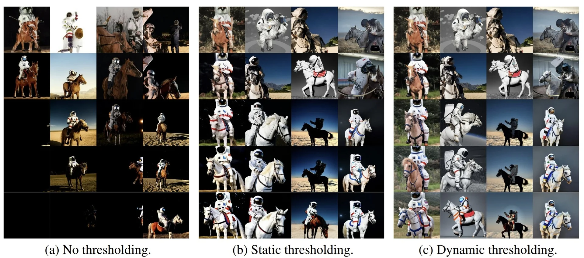
Experimental Findings and DrawBench Evaluation
Scaling the Text Encoder A central insight of Imagen [557] is that text encoder quality is a dominant factor in text-to-image generation. In systematic ablations, the authors vary the underlying language model used to encode the caption—comparing T5-Base, T5-Large, T5-XL, and T5-XXL—and observe consistent improvements in both image-text alignment and visual fidelity as model size increases.
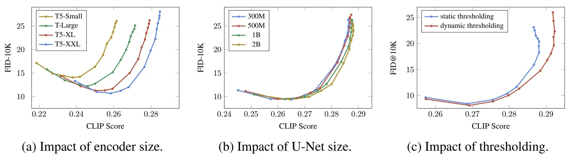
These results motivate a design shift: instead of primarily scaling the image generator (as done in prior works), Imagen prioritizes high-capacity language understanding, even when the encoder is frozen during training. This strengthens the mapping from prompt to semantic features, yielding more accurate and coherent visual generations.
DrawBench: A Diverse Prompt Evaluation Suite To evaluate generative performance beyond cherry-picked prompts, the authors introduce DrawBench, a human preference-based benchmark of 200 prompts spanning multiple semantic categories:
- Object and scene composition
- Spatial relationships and counting
- Style and texture
- Complex language grounding
Each model (e.g., Imagen, DALL\(\cdot \)E 2, GLIDE, LDM, VQGAN+CLIP) generates images for each prompt, which are then compared in a blind A/B format for:
- Alignment: Does the image accurately reflect the text prompt?
- Fidelity: Is the image visually plausible and high-quality?
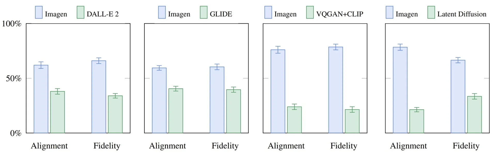
Imagen significantly outperforms the baselines on both axes, demonstrating the effectiveness of its text encoder, CFG tuning, and cascading architecture.
Qualitative Samples Finally, the model produces diverse, photorealistic samples across various creative and grounded prompts:
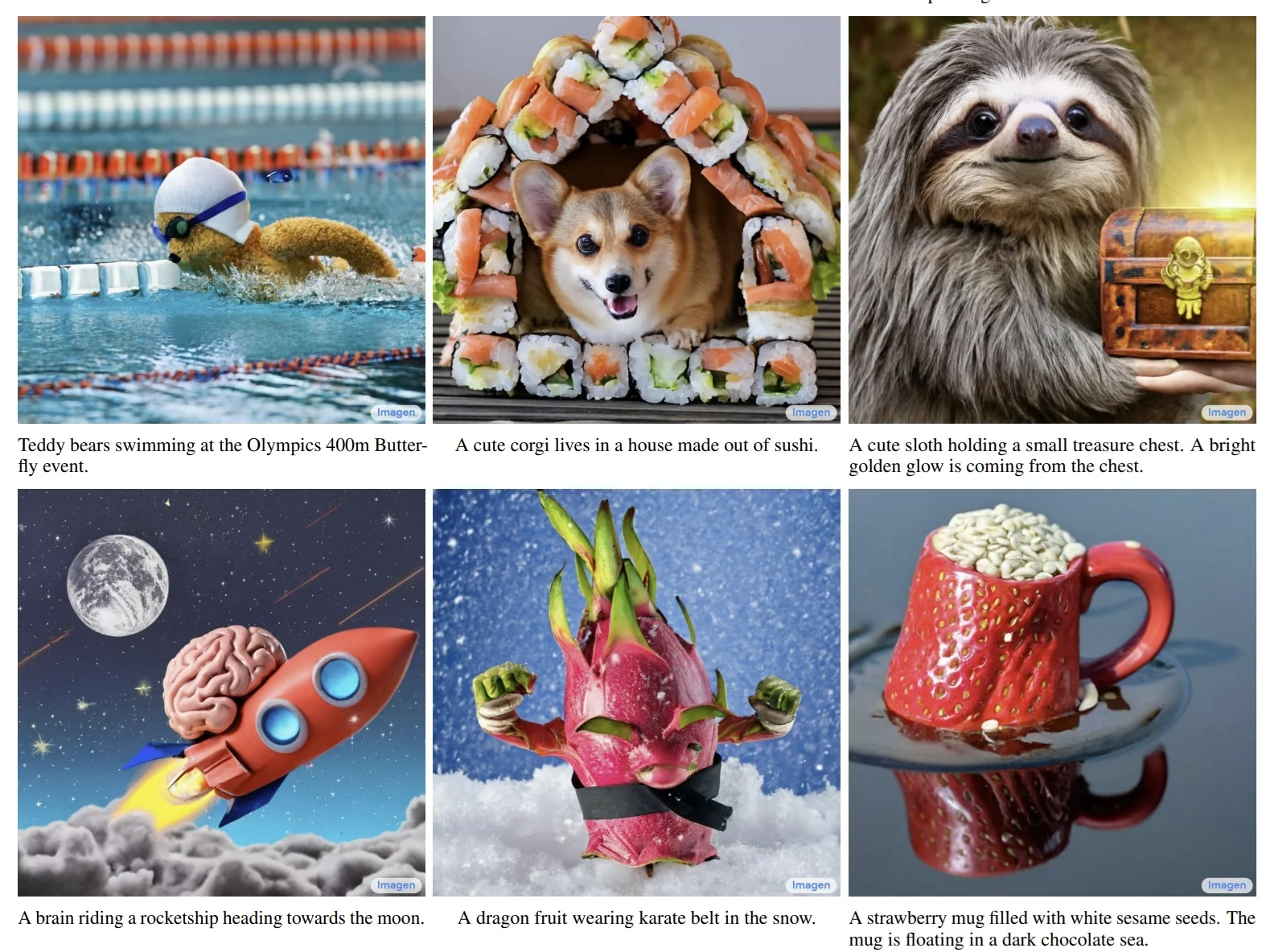
Enrichment 20.11.5.1: Toward Fine-Grained Control and Editable Generation
From Fidelity to Controllability While models like Imagen [557] and DALL\(\cdot \)E 2 [524] have achieved remarkable success in photorealism and semantic alignment, they remain fundamentally non-interactive. Once an image is generated from a text prompt, the process is opaque: users have no control over which elements change if the prompt is revised.
This poses a major limitation in creative and iterative workflows. For example, a designer modifying the prompt from “a red car” to “a blue car” expects only the car’s color to change, while preserving the original composition, lighting, and style. In practice, however, standard diffusion pipelines—including those using classifier-free guidance (CFG)—often regenerate the image from scratch, with unpredictable changes to unrelated regions.
Why Prompt-Aware Attention Control Is Needed To address this, recent work focuses on editable generation—where models support localized updates, identity preservation, and deterministic user control. Three key goals underpin this new research direction:
- Fine-grained editability: Allow prompt-based modifications (e.g., changing “cat” to “dog”) without altering unrelated image regions.
- Semantic preservation: Maintain critical attributes such as object identity, layout, and lighting even after prompt edits.
- Interactive control: Introduce modular control signals—like segmentation masks, edge maps, or pose estimations—that act as “handles” for spatial or structural guidance.
Key Approaches and Innovations A growing ecosystem of techniques now forms the foundation for controllable diffusion-based generation—each offering distinct mechanisms for enabling user-guided synthesis:
- Prompt-to-Prompt (P2P) [226]: Introduces a novel method for prompt-driven editing by intervening in the model’s cross-attention maps during inference. Instead of retraining or re-encoding, it aligns attention weights across similar prompts to preserve spatial layout and object identity. This enables intuitive text modifications (e.g., “red shirt” to “blue shirt”) that affect only relevant regions, without disturbing the rest of the image.
- DreamBooth [554]: Targets personalization by finetuning a pretrained diffusion model on a small set of subject-specific images, anchored to a rare textual token (e.g., “sks”). This allows generation of images that retain the subject’s identity across diverse scenes and poses—crucial for creative professionals, avatars, or character preservation tasks.
- ControlNet [794]: Enables structural conditioning through auxiliary inputs like pose skeletons, depth maps, or edge detections. Crucially, it does so without modifying the base model by injecting trainable control paths that are fused with the original network. This unlocks precise spatial control and makes diffusion adaptable to external guidance from perception pipelines or user interfaces.
- IP-Adapter [755] and Transfusion [818]: Introduce modular, plug-and-play conditioning layers designed to adapt pretrained diffusion models to new visual or multimodal signals—without modifying the original weights. IP-Adapter uses a decoupled cross-attention mechanism that injects CLIP-derived image embeddings alongside frozen text features, enabling flexible image-guided generation, personalization, and cross-modal editing with only 22M trainable parameters. Transfusion builds on this adapter paradigm by unifying visual grounding with text and sketch modalities, enabling diverse zero-shot edits across tasks. Both approaches preserve the underlying text-to-image capabilities, making them well-suited for scalable, reusable, and composable image generation pipelines.
Collectively, these methods reframe diffusion models as interactive generation systems—capable of fine-grained control, identity preservation, and user-driven customization. The following sections delve into these approaches, starting with Prompt-to-Prompt, which introduced one of the first scalable solutions for semantically coherent prompt editing without sacrificing layout or visual consistency.
Enrichment 20.11.6: Prompt-to-Prompt (P2P): Cross-Attention Editing in DMs
Motivation and Core Insight Prompt-to-Prompt (P2P) [226] introduces a novel method for fine-grained, prompt-based image editing in text-to-image diffusion models. Unlike prior approaches that either operate directly in pixel space or require full model finetuning, P2P achieves precise semantic control by modifying only the prompt and reusing internal cross-attention maps of the diffusion process.
The core insight is that in text-conditioned diffusion models (e.g., Stable Diffusion), each token in the prompt corresponds to a spatial attention map over the latent image at every denoising step. These maps govern “what part of the image is controlled by which word”. By injecting stored attention maps for shared tokens between an original and edited prompt, P2P preserves image structure while applying meaningful semantic changes.
This mechanism allows users to:
- Replace entities (e.g., “a cat” \(\rightarrow \) “a dog”) while preserving the scene layout.
- Modify stylistic details (e.g., “a photo of a mountain” \(\rightarrow \) “a charcoal drawing of a mountain”).
- Tune the emphasis of individual adjectives or objects (e.g., increasing the visual weight of “snowy”).
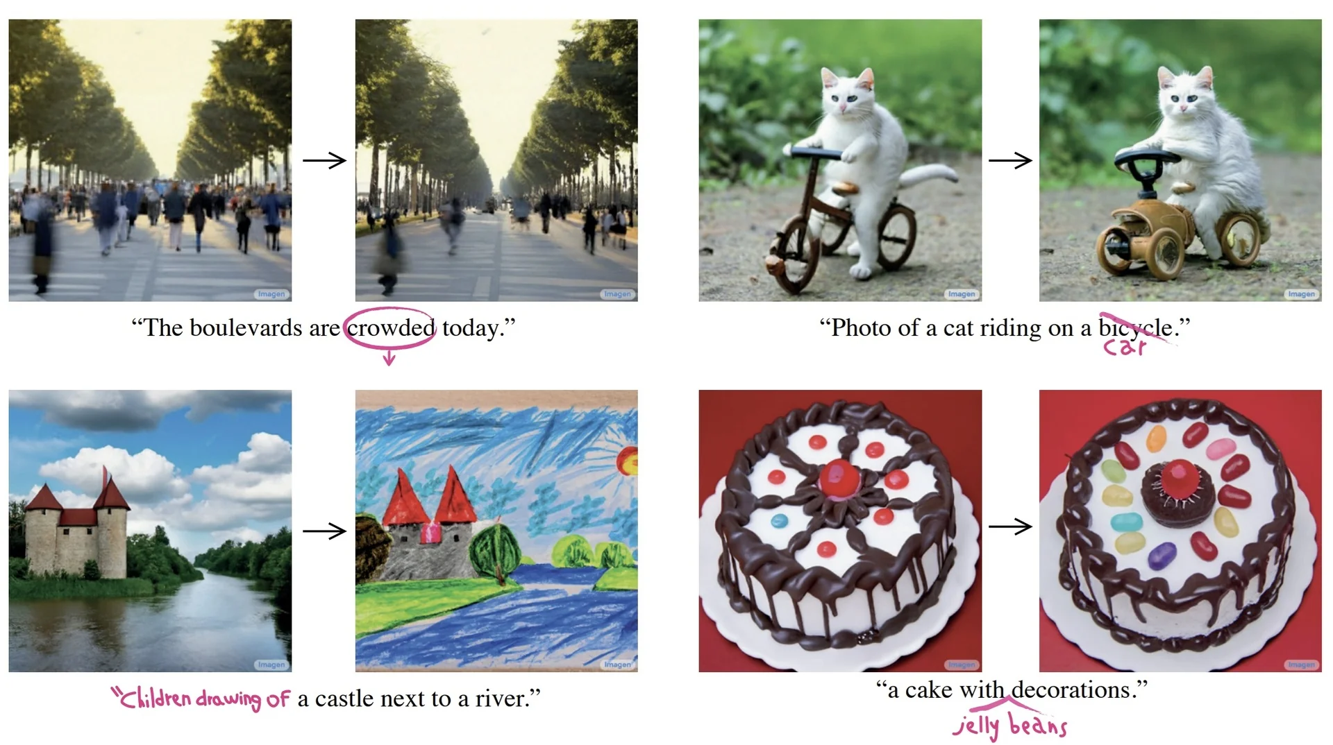
P2P thus bridges the flexibility of prompt-based conditioning with the structural fidelity of spatial attention, enabling zero-shot edits with pixel-level consistency. In the following, we will explain how this method works, and see some usage examples.
Cross-Attention as the Mechanism for Prompt Influence In text-conditioned diffusion models such as Stable Diffusion, the U-Net backbone integrates the prompt via cross-attention layers at every denoising step \( t \in \{1, \dots , T\} \). At each step, the model maintains a latent representation \( \vec {z}_t \in \mathbb {R}^{h \times w \times d} \), where each of the \( N = h \cdot w \) spatial locations corresponds to a feature vector of dimension \( d \). This tensor is reshaped into a sequence \( \vec {z}_i \in \mathbb {R}^{N \times d} \), where each row \( \vec {z}_i[n] \) can be interpreted as encoding local information at spatial location \( n \) — similar to a pixel in a feature map, though potentially corresponding to a receptive field in the original image due to earlier convolutional layers.
Let the text prompt be tokenized into \( L \) tokens, each embedded into a vector \( \vec {e}_l \in \mathbb {R}^d \), forming an embedding matrix \( \vec {E} \in \mathbb {R}^{L \times d} \). These embeddings serve as the key-value memory bank over which the latent queries will attend. The cross-attention computation at each U-Net layer is then given by:
\[ \mbox{Attention}(\vec {z}_i, \vec {E}) = \mbox{softmax} \left ( \frac {Q K^\top }{\sqrt {d}} \right ) V, \]
where:
- \( Q = W_Q \vec {z}_i \in \mathbb {R}^{N \times d} \) are learned linear projections of the spatial feature vectors — one per location \( n \),
- \( K = W_K \vec {E}, \quad V = W_V \vec {E} \in \mathbb {R}^{L \times d} \) are the projected keys and values from the prompt token embeddings,
- \( A^t = \mbox{softmax} \left ( Q K^\top / \sqrt {d} \right ) \in \mathbb {R}^{N \times L} \) is the attention matrix at timestep \( t \).
If the original channel dimensions of \( \vec {z}_i \) or \( \vec {E} \) differ, the projections \( W_Q, W_K, W_V \) are used to map both inputs into a shared dimension \( d \), ensuring compatibility. These are learnable parameters trained end-to-end with the diffusion model.
Each entry \( A^t[n, l] \) quantifies how much the token \( w_l \) influences the generation at spatial position \( n \). This allows us to interpret the model as dynamically querying which parts of the prompt should affect which spatial regions of the latent representation.
We define the cross-attention map for token \( w_l \) at timestep \( t \) as: \[ M_l^t := A^t[:, l] \in \mathbb {R}^{N}, \] where \( A^t \in \mathbb {R}^{N \times L} \) is the cross-attention matrix at timestep \( t \), with \( N = h \times w \) denoting the number of spatial locations in the latent feature map and \( L \) the number of text tokens. The slice \( A^t[:, l] \) selects the attention weights from all spatial positions to the token \( w_l \), yielding a heatmap over image space that describes how strongly each location attends to the semantic concept expressed by \( w_l \).
This vector \( M_l^t \) can be reshaped into a 2D grid \( M_l^t \in \mathbb {R}^{h \times w} \) to match the spatial resolution of the U-Net features, allowing a visual interpretation of where token \( w_l \) is grounded at step \( t \). For example, if \( w_l = \mbox{``dog''} \), the corresponding map \( M_l^t \) will have high values in regions corresponding to the predicted dog’s body, such as its head or torso.
Concretely, if a spatial location \( i = (u, v) \) on the feature map has a high value \( M_l^t[u, v] \), it indicates that the pixel at location \( (u, v) \) in the latent representation is currently being influenced by, or aligned with, the semantics of the word “dog”. Thus, the cross-attention map captures the evolving alignment between text tokens and spatial regions throughout the diffusion process, enabling localized text-to-image control.
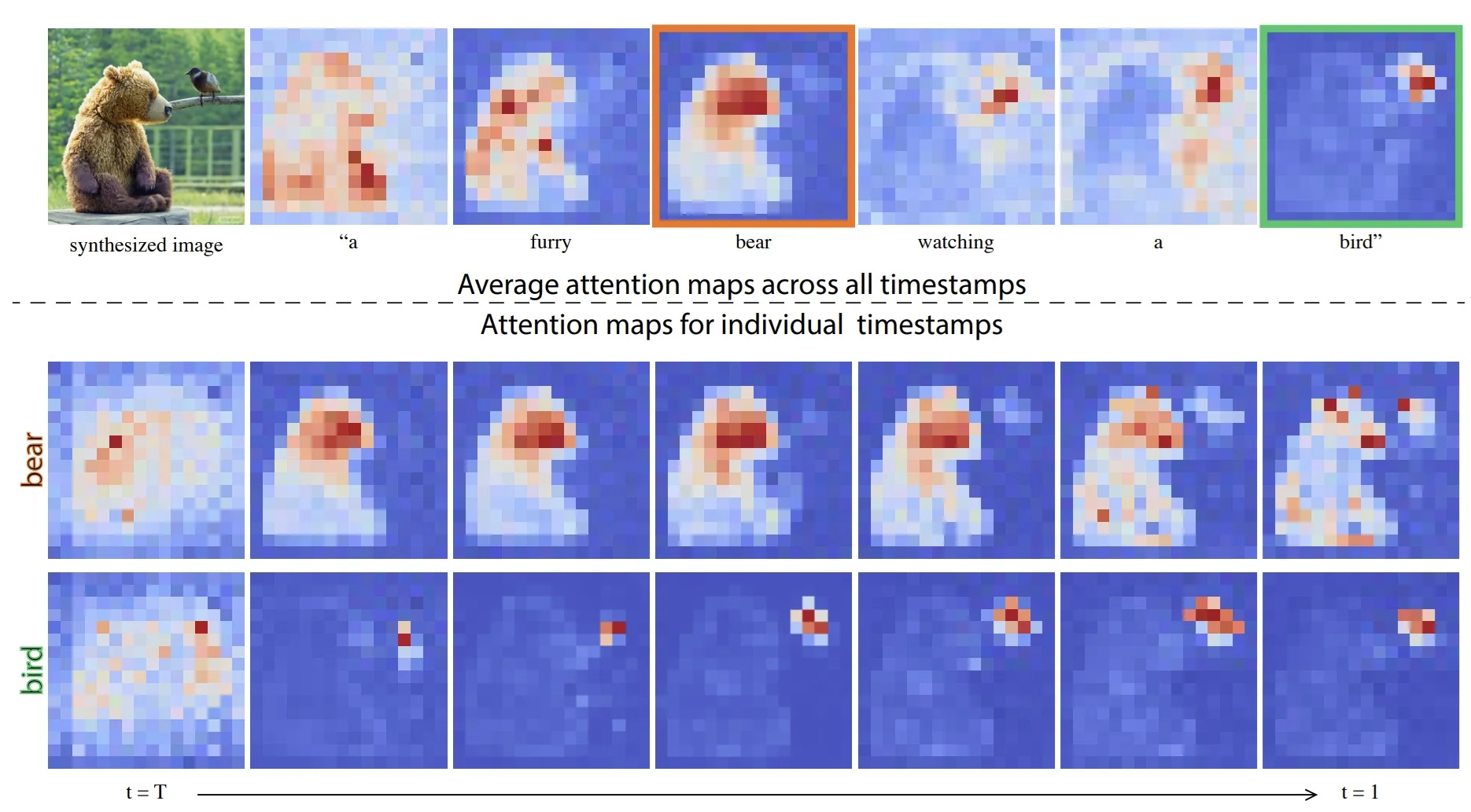
This attention mechanism forms the foundation for Prompt-to-Prompt’s editing capabilities: by storing the maps \( M_l^t \) from an initial prompt and reusing them selectively during generation with a modified prompt, one can tightly control how semantic concepts from the original image persist or change across edits. The next part describes how this editing mechanism is implemented.
Editing by Cross-Attention Injection Prompt-to-Prompt (P2P) [226] enables fine-grained, prompt-aware image editing by intervening in the cross-attention maps of a pre-trained text-to-image diffusion model. Given an original prompt \({p} = [w_1, \dots , w_L] \) and a revised prompt \({p}' = [w_1', \dots , w_{L'}'] \), the method aligns their token sequences and selectively manipulates attention maps \( M_l^t \) across diffusion timesteps \( t \in \{1, \dots , T\} \).
The core intuition is straightforward: each token \( w_l \) in the prompt attends to a spatial region in the image via its attention map \( M_l^t \), which evolves over time. If a token remains unchanged across prompts—e.g., “tree” in “a dog next to a tree” versus “a cat next to a tree”—then its associated spatial influence should also remain fixed. P2P enforces this consistency by injecting attention maps recorded during generation with the original prompt into the diffusion process guided by the new prompt.
By doing so, the method preserves image layout and semantic grounding for shared tokens, while allowing newly introduced or modified tokens to affect the image selectively.
This form of editing occurs at the cross-attention layers within the U-Net and can be controlled over time using a timestep threshold \( \tau \), enabling smooth interpolation between preservation and change.
The key components are:
- Attention Replacement for Matching Tokens: When a token \( w_l \in {p} \) appears identically in the edited prompt \( {p}' \), its attention map is replaced with the one recorded during generation of the original image: \[ M_l^{\prime t} \leftarrow M_l^t. \] This preserves the spatial layout and semantic grounding of the unchanged concept (e.g., “table” in both prompts “a red chair and a table” and “a blue chair and a table”).
-
Word Swapping via Timestep-Gated Attention Injection:
When a token in the prompt is replaced—for example, “car” \( \rightarrow \) “truck”—the goal is to modify the generated concept while keeping the rest of the image (e.g., layout, background, lighting) structurally intact. Prompt-to-Prompt (P2P) achieves this via a timestep-gated injection of cross-attention maps, controlled by a parameter \( \tau \), applied during the denoising process.
How it works: Diffusion models denoise a latent representation iteratively. At each timestep \( t \), cross-attention layers in the U-Net bind the current visual features (queries) to text tokens (keys and values). The resulting attention map \( M_l^t \in \mathbb {R}^{h \times w} \) for token \( w_l \) determines how strongly each spatial location should attend to that token.
Importantly, these maps encode where in the image each token is relevant—but not what the token means. The token’s semantic identity is carried through its embedding \( \vec {v}_l \), projected into the attention’s value vectors \( V \). During cross-attention, each spatial location receives a weighted sum of the values, using the attention map as weights: \[ \mbox{Output} = \hat {M}_l^t \cdot V_l^{\prime } \] In word swapping, P2P modifies the attention maps \( \hat {M}_l^t \) as follows: \[ \hat {M}_l^t = \begin {cases} M_l^{\prime t} & \mbox{if } t < \tau \quad \mbox{(use attention map from the new prompt)} \\ M_l^t & \mbox{if } t \geq \tau \quad \mbox{(inject original map from the old prompt)} \end {cases} \]
Why it works: Early in the diffusion process, the model determines the coarse structure—object layout, pose, and geometry. Using \( M_l^{\prime t} \) here ensures the new token (e.g., “truck”) can shape its own spatial identity, learning its approximate location and structure. Crucially, the values \( V_l^{\prime } \) always come from the new token embedding, so the semantic content being drawn from is never related to the original token (“car”).
Later in the process (\( t \geq \tau \)), the model begins refining texture, shading, and scene consistency. At this point, P2P injects the original attention maps \( M_l^t \) while still using the new values \( V_l^{\prime } \). This means the model is now told: “inject the semantic content of a truck, but do so in the spatial pattern where a car originally appeared.”
This is the crucial trick: the new concept (truck) inherits the spatial context of the old concept (car)—its location, size, and perspective—but none of its identity. There is no semantic leakage from the original word because the values, which carry the detailed information injected into the visual features, still come from the new prompt.
Example: When editing “a red sports car on a road” into “a red truck on a road,” early timesteps allow the attention of “truck” to shape its own geometry. After \( \tau \), the attention map of the original “car” is re-used, telling the model where in the image to continue refining. The resulting truck is structurally aligned with the original car’s pose and lighting, yet semantically distinct.
About the parameter \( \tau \): The transition point \( \tau \in [0, T] \) determines when control shifts from free composition to spatial anchoring. A smaller \( \tau \) gives more influence to the new prompt, allowing larger structural changes. A larger \( \tau \) preserves more of the original layout. In practice, intermediate values (e.g., \( \tau \approx 0.5 T \)) often strike a balance between visual fidelity and effective editing.
-
Adding New Phrases:
Suppose we augment the prompt from “a house in the snow” to “a house in the snow with a tree”. Our goal is to preserve the existing content (house, snow) while introducing the new concept (tree) in a natural and non-destructive way.
How it works: Let \( {p} \) and \( {p}' \) denote the original and edited prompts, respectively. At each timestep \( t \), Prompt-to-Prompt constructs the edited cross-attention maps \( \hat {M}_l^t \) as follows:
- For each token \( w_l \in {p} \cap {p}' \) that appears in both prompts, we inject the original attention map: \[ \hat {M}_l^t := M_l^t. \] This enforces spatial consistency for the unchanged concepts (e.g., “house”, “snow”).
- For each newly added token \( w_l \in {p}' \setminus {p} \), such as “tree”, we allow the model to compute its attention map normally: \[ \hat {M}_l^t := M_l^{\prime t}. \]
Why it usually works: This approach biases the generation toward preserving the original structure while carving out visual space for the new concept. The success of this balance depends on three factors:
- Preserved attention anchors: By freezing the attention maps for shared tokens, we ensure that their semantic influence remains fixed over the original image regions. This strongly encourages the model to reconstruct those regions similarly in the edited version.
- Limited interference by new tokens: Although new tokens can, in principle, influence any part of the image, their attention is typically focused on previously unclaimed or neutral areas—such as background space—where the frozen maps from shared tokens are weak. This is due to softmax normalization: strong attention weights from shared tokens crowd out competing influence from new ones in key regions.
- Value-weighted blending: Even when spatial attention overlaps, the injected attention maps act only as weights. The semantic content injected at each position still comes from the values—i.e., the token embeddings. Since the new token (“tree”) has distinct values from existing ones, its content will only dominate in regions where it receives sufficient attention. In most cases, this naturally confines it to appropriate areas without harming other objects.
Important caveat: This method is not foolproof. If a new token’s attention overlaps heavily with a shared token’s region, and its values inject strong or conflicting semantics, artifacts or unintended modifications can occur. However, such cases are rare in practice, especially for prompts that are incrementally edited or composed of semantically separable elements. Fine-tuning the diffusion guidance strength or manually constraining attention can further mitigate these risks.
Example: Inserting “a tree” into “a house in the snow” results in a tree appearing beside the house—often in the background or foreground—without shifting or deforming the house itself. The spatial layout and visual style of the original scene are preserved because the attention maps for “house” and “snow” remain fixed, shielding those areas from disruption.
-
Attention Re-weighting (Optional):
In prompts containing multiple concepts—such as “a cat on a chair with sunlight in the background”—we may wish to emphasize or suppress specific elements. For instance, one might want to intensify “sunlight” to brighten the scene or reduce the visual clutter associated with “background”. Prompt-to-Prompt enables this via a technique called attention re-weighting, also referred to as fader control.
How it works: Let \( j^* \) denote the index of the token to be modified, and let \( c \in [-2, 2] \) be a scaling coefficient. At each diffusion step \( t \), the cross-attention map \( M^t \in \mathbb {R}^{N \times L} \) from the original prompt’s generation is reweighted to obtain \( \hat {M}^t \), where each spatial position \( i \in \{1, \dots , N\} \) attends over the \( L \) tokens: \[ \hat {M}_{i,j}^t := \begin {cases} c \cdot M_{i,j}^t & \mbox{if } j = j^* \\ M_{i,j}^t & \mbox{otherwise} \end {cases} \] After reweighting, each row \( \hat {M}_{i,:}^t \) is typically renormalized (e.g., using softmax) to ensure the attention remains a valid distribution.
Why it works: Cross-attention determines where each token’s semantics are injected into the latent image during denoising. The weights \( M_{i,j}^t \) are used to combine the value vectors \( \vec {v}_j \) (from the token embeddings), controlling how much each token contributes at location \( i \). Increasing \( c \) boosts the pre-softmax score for token \( j^* \), which raises its relative weight after softmax: \[ \mbox{Softmax}(\hat {M}_{i,:}^t)[j^*] = \frac {e^{c M_{i,j^*}^t}}{\sum _{k=1}^{L} e^{\hat {M}_{i,k}^t}}. \] Thus, more pixels are drawn to the token’s semantic content, strengthening its influence. Conversely, reducing \( c \) weakens this effect.
Why it usually doesn’t disrupt other objects: Reweighting adjusts only a single token’s attention column. Since the attention is row-wise normalized, boosting one token proportionally reduces others—but only at spatial locations where that token already had influence. For unrelated concepts with disjoint spatial support, the impact is minimal. That said, large \( c \) values can overpower neighboring tokens in shared regions, potentially distorting their features.
Example: Increasing \( c \) for “sunlight” enhances brightness across attended regions, reinforcing highlights and atmospheric glow. Suppressing “background” with a low \( c \) reduces texture variation and visual noise, producing a cleaner, more focused composition.
These operations allow users to perform prompt-level edits—such as word substitution, phrase addition, or semantic emphasis—while preserving coherence, layout, and object identity in the image. Crucially, attention injection is not applied uniformly across the entire generation: the timestep threshold \( \tau \) allows for nuanced control over when the structure should be preserved and when it can adapt, striking a balance between faithfulness and flexibility.
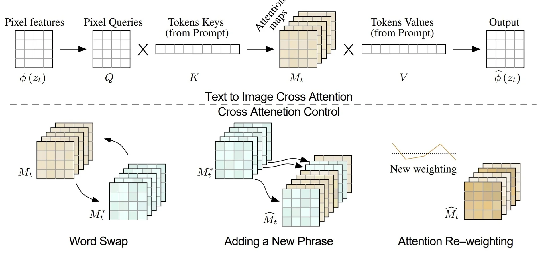
This mechanism is particularly effective because it leverages the spatial grounding inherent in attention maps: regions influenced by unchanged words remain fixed, while edited words influence only localized changes. This permits high-fidelity image editing without requiring pixel-space operations or model retraining.
In the following, we demonstrate how this mechanism can modify object content, style, or structure while preserving layout.
Use Case: Content Modifications via Prompt Edits Once the Prompt-to-Prompt mechanism is in place, a natural application is controlled object substitution through prompt editing. For example, replacing “lemon cake” with “chocolate cake” or “birthday cake” should change only the appearance of the object itself while preserving the layout, lighting, and background structure.
The below figure demonstrates this use case. Starting from a baseline image generated from the prompt “lemon cake”, the prompt is modified to describe other cake types. Two editing strategies are compared:
- Top row (attention injection): P2P preserves the spatial layout of all shared words by copying their attention maps from the original generation. Only new tokens receive fresh attention maps.
- Bottom row (seed reuse only): The same random seed is reused, but no attention maps are injected — each prompt is generated independently.
In the attention-injected row, the cake’s pose, size, and plate remain stable across edits — the structure is preserved, and only semantic details (like texture and topping) change. Without attention injection, the geometry drifts significantly, resulting in inconsistent layouts.
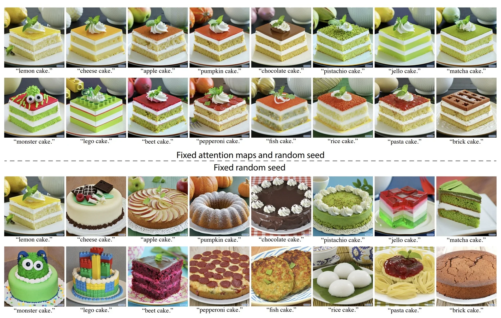
This example highlights Prompt-to-Prompt’s ability to perform semantic transformations while preserving the geometric footprint of unchanged content — a key feature for controlled editing in image synthesis workflows.
We now turn to further use cases demonstrating Prompt-to-Prompt’s flexibility, including object preservation across scene changes, gradual injection strength for stylistic blending, and real-image editing via inversion.
Use Case: Object Preservation Across Scene Changes Prompt-to-Prompt also supports isolating and preserving a specific object from a source image while altering the rest of the scene. This is accomplished by selectively injecting the attention maps corresponding to a single token, such as “butterfly”, from the original prompt.
The below figure demonstrates how injecting only the attention maps of the word “butterfly” preserves its pose, structure, and texture across multiple edited prompts. The new contexts vary in composition and background — e.g., a room, a flowerbed, or abstract shapes — but the butterfly remains visually consistent, accurately positioned, and realistically integrated.
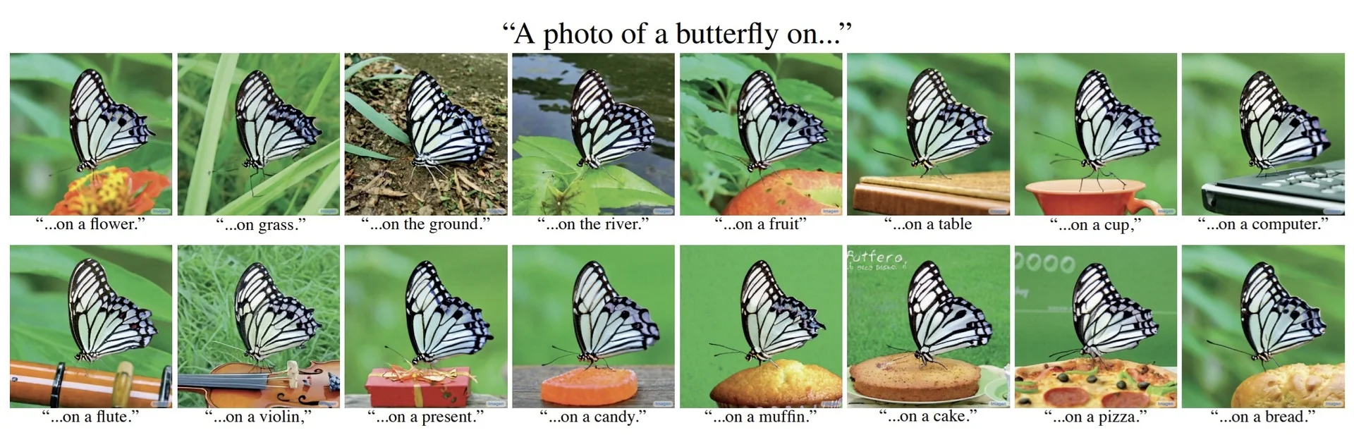
This type of localized control is especially useful for identity-preserving edits or compositional consistency — applications relevant to character animation, creative storytelling, and personalized image manipulation. It also sets the stage for more advanced use cases involving dynamic modulation of attention influence and real-image editing.
Use Case: Controlled Blending via Partial Attention Injection Prompt-to-Prompt enables fine-grained control over the generation process by specifying the temporal extent during which the original cross-attention maps are injected. By limiting attention replacement to only a subset of denoising timesteps \( \tau \in [0, T] \), users can navigate the trade-off between faithfulness to the edited prompt and fidelity to the original image structure.
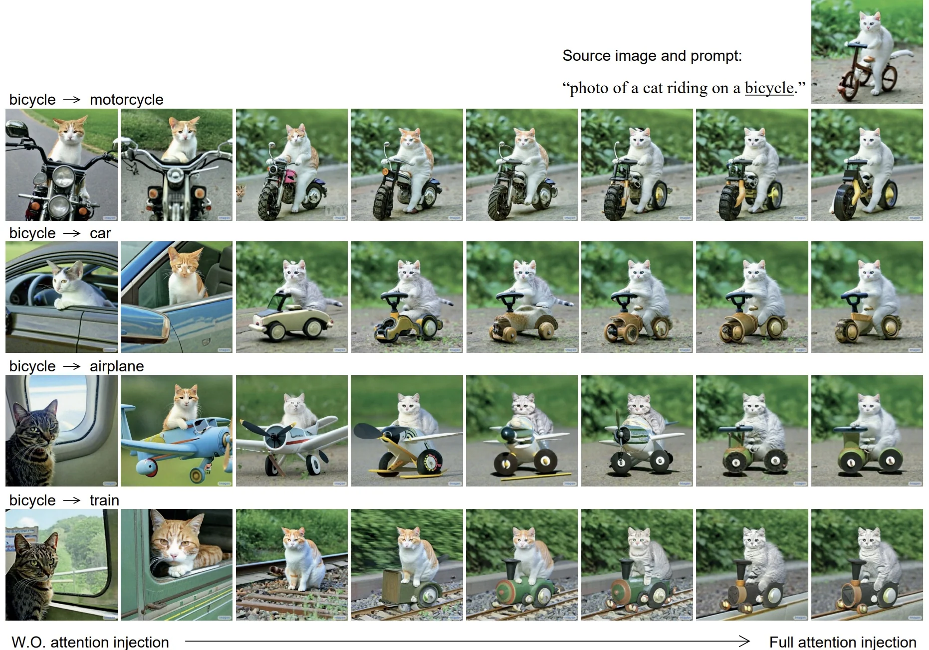
Mechanism of control: Let \( \tau \in [0, T] \) be the timestep threshold at which attention injection transitions. For timesteps \( t < \tau \), the cross-attention maps computed from the edited prompt are used (encouraging semantic changes); for \( t \geq \tau \), the maps from the original prompt are injected (enforcing structural consistency). A small \( \tau \) means most steps rely on the original attention, preserving layout but potentially suppressing edits. A large \( \tau \) allows the new token’s semantics to dominate, which may yield better object replacement but increase spatial drift.
Why it matters: This mechanism allows users to blend the “what” (new concept) and “where” (original spatial anchors) over time, rather than committing to full replacement or preservation. For instance, replacing “car” with “bicycle” may succeed when injection occurs only after the early timesteps—letting the bicycle establish geometry, then snapping into the original scene’s pose and viewpoint.
This time-dependent attention editing proves useful in scenarios where both semantic change and structural stability are important. Applications include identity-preserving edits, fine-grained modifications to clothing or pose, and stylistic alterations that should respect background composition.
We now turn to complementary editing strategies that do not replace attention maps, but instead reweight them to modulate a token’s influence.
Use Case: Emphasizing and De-emphasizing Concepts Building on the principle of attention re-weighting, Prompt-to-Prompt enables dynamic emphasis or suppression of specific concepts directly through cross-attention manipulation. This allows users to subtly or dramatically control how visible or dominant a particular word becomes in the generated image—without changing the wording of the prompt itself.
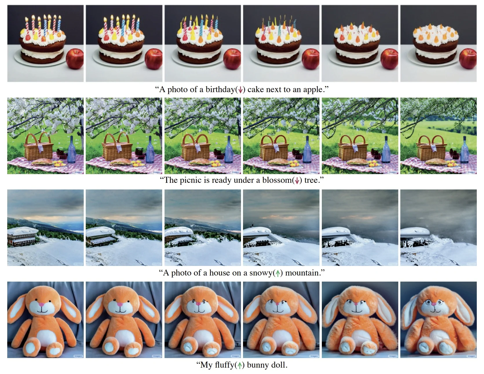
In Figure 20.106, re-weighting is applied to highlight or downplay specific concepts. For example, increasing the attention mass on the token “fluffy” causes the entire image to exhibit more fluffiness in the texture of objects (in this example, the furry bunny doll). Conversely, reducing the attention weight on “blossom” attenuates the flower density and vibrancy of the tree canopy.
This flexible form of text-guided emphasis is useful in stylization, mood control, and semantic adjustment without prompt rewriting. The same technique can be applied for creative stylization.
Use Case: Text-Guided Stylization while Preserving Layout Prompt-to-Prompt enables text-guided stylization, allowing users to transform an image’s appearance while maintaining its spatial composition and semantic structure. This is achieved by appending stylistic descriptors (e.g., “charcoal sketch”, “futuristic illustration”) to the prompt while injecting the cross-attention maps from the original prompt. These injected maps anchor spatial localization, ensuring that stylistic changes affect only visual texture, tone, and color, not layout.
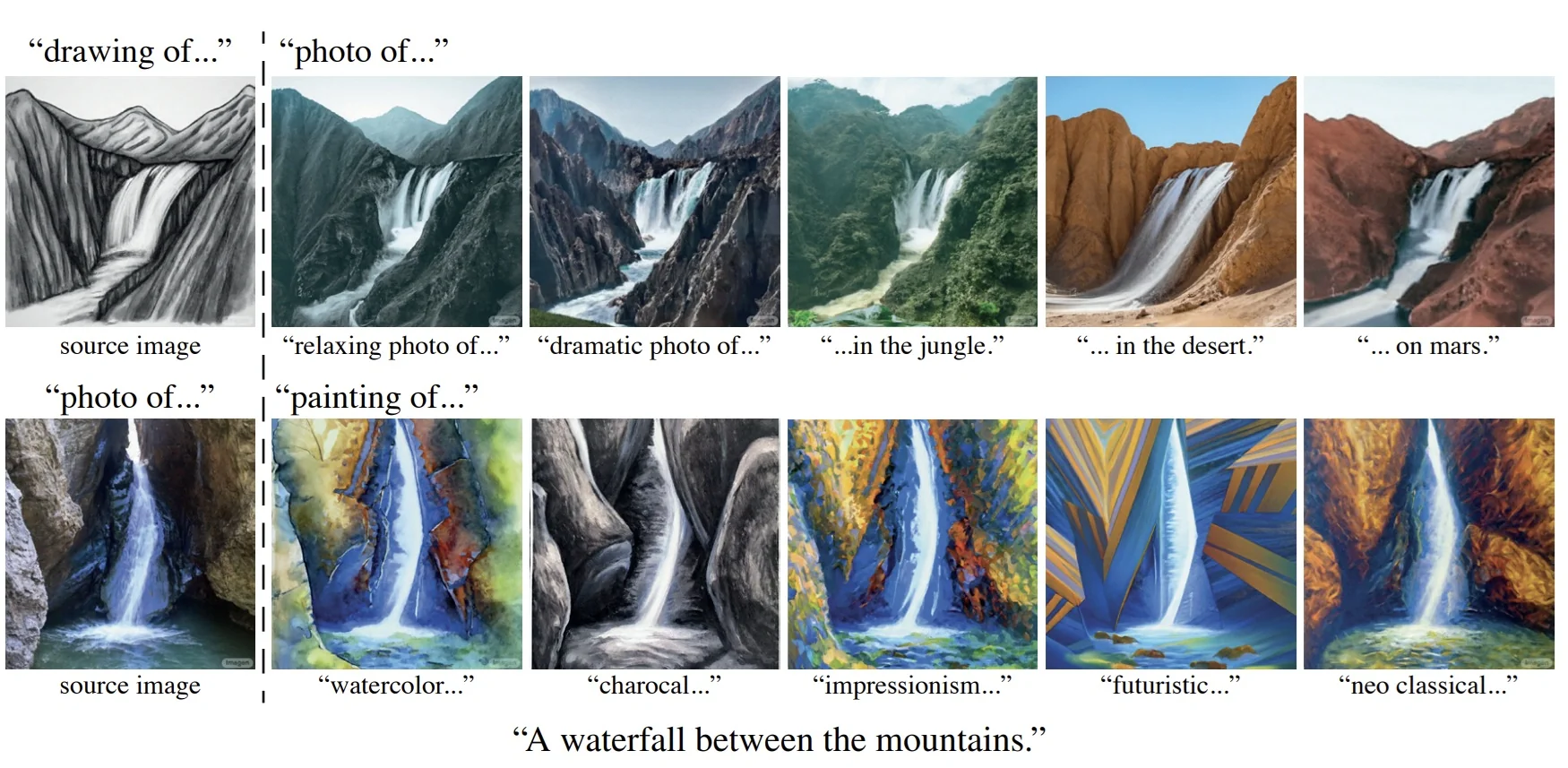
This strategy supports both sketch-to-photo and photo-to-sketch transformations, modulated entirely through text. By preserving structural attention, Prompt-to-Prompt ensures that stylistic changes remain localized to appearance, enabling faithful reinterpretations of the same scene across diverse visual domains. Such capabilities are valuable for domain adaptation, visual exploration, and iterative artistic workflows—offering a controllable, prompt-driven alternative to manual stylization or style transfer networks.
Use Case: Editing Real Images via Inversion and Prompt-to-Prompt Finally, Prompt-to-Prompt is not limited to synthetic images. By leveraging diffusion inversion techniques (e.g., DDIM inversion), real images can be mapped into latent noise vectors and edited as if they were generated samples. This extends the power of prompt-based editing to real-world inputs.
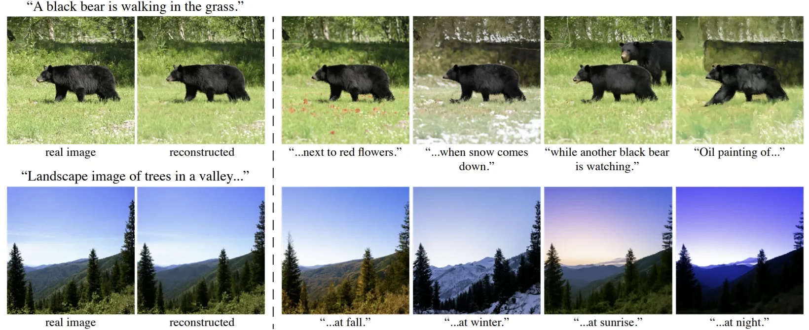
As shown in Figure 20.108, the inversion step maps a real photo (e.g., of a dog, house, or object) into a latent representation from which a faithful reconstruction can be generated. Prompt edits—such as changing the subject, adjusting appearance, or adding stylistic elements—are then applied via P2P. The result is an edited image that respects the original structure and layout but incorporates the semantic changes described in the updated prompt.
This capability opens the door to user-friendly image editing pipelines where real images can be modified through text alone, with fine-grained control over structure and content.
Limitations and Transition to Personalized Editing While Prompt-to-Prompt offers fine-grained control over textual edits through cross-attention injection, re-weighting, and temporal scheduling, it still inherits several limitations from the underlying diffusion framework:
- Vocabulary-bound concept control: P2P assumes that all visual elements in the scene are represented by prompt tokens. Consequently, it cannot edit or preserve objects that lack a direct textual grounding—such as a specific person’s face, a custom logo, or a unique product design.
-
Semantic drift with underrepresented concepts: For rare or ambiguous tokens (e.g., “blossom”, “rustic”, or abstract modifiers like “ethereal”), the associated value vectors may not fully capture the desired visual features. As a result, cross-attention editing may be inconsistent, yielding unpredictable outputs or semantic drift over time.
- Limited identity preservation: Because Prompt-to-Prompt relies purely on manipulating cross-attention weights, it cannot preserve fine-grained visual identity—such as the facial features of a specific subject—when editing real images. As demonstrated in prior sections, even when using DDIM inversion to anchor the source image in latent space, significant details may be lost or altered during generation.
These limitations motivate the need for personalized fine-tuning techniques that go beyond attention manipulation. In particular, to faithfully edit scenes involving novel or user-defined subjects—such as a specific dog, a unique sculpture, or a person’s face—we require models that can learn new visual concepts and bind them to custom textual tokens.
While Prompt-to-Prompt enables fine-grained control over structure and style through attention manipulation, it remains limited to concepts already understood by the base model. It cannot synthesize entirely new identities or visually-grounded concepts absent from the training data. This motivates the need for subject-driven generation, where the model is explicitly taught to recognize and recreate a particular instance—such as a person, object, or pet—across diverse prompts and settings.
This leads us to DreamBooth [554], a technique for high-fidelity personalization via instance-specific fine-tuning. DreamBooth introduces a unique token (e.g., “[V]”) into the model’s vocabulary and trains the model to associate it with the visual identity of a particular subject using just a handful of example images. Once embedded, this token can be flexibly composed with other text descriptors to guide generation across different poses, environments, and styles—all while preserving core identity traits.
In the following, we explore how DreamBooth achieves this level of instance control, what challenges arise in balancing identity preservation with prompt diversity, and how its innovations laid the groundwork for personalized diffusion models.
Enrichment 20.11.7: DreamBooth: Personalized Text-to-Image Generation
Motivation and Core Insight DreamBooth [554] proposes a method for customizing pretrained text-to-image diffusion models—such as Stable Diffusion or Imagen—so that they can generate realistic, context-aware, and stylistically diverse images of a specific subject, using only a handful of example images.
The key challenge addressed by DreamBooth is as follows: while large diffusion models are trained on broad distributions of internet-scale data, they cannot reliably synthesize faithful renditions of an individual subject (e.g., a specific dog or product) unless it appeared in their training data, and with a unique identifier that allows reconstruction in various settings. Simply prompting with ”a dog on a beach” might yield a generic canine, but not your dog.
To solve this, DreamBooth introduces the idea of binding a unique textual identifier—such as sks—to a novel visual subject by fine-tuning the diffusion model on a small set of subject-specific images paired with customized prompts (e.g., ”a photo of a sks dog”). This enables the model to learn the association between the identifier and the subject’s visual concept, allowing the generation of high-fidelity outputs in new poses, scenes, or styles using just prompt-based control.
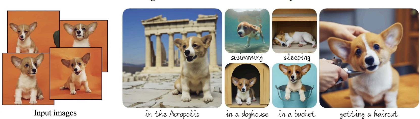
This mechanism builds toward a more general idea in controllable generation: associating visual attributes with tokens in the text space and using prompt engineering to drive structured edits. In later works, we will see how ControlNet extends this idea further by conditioning on spatial inputs like edges or poses. But first, we will examine how DreamBooth establishes the foundational capability of subject-driven customization using only a few images and simple text.
Model Setup and Identifier Creation DreamBooth [554] modifies large pretrained text-to-image diffusion models—such as Stable Diffusion and Imagen—to enable personalized subject-driven generation. Given only a handful of subject reference images (typically 3–5), DreamBooth introduces a new textual identifier that serves as a symbolic stand-in for the subject. By finetuning the model on prompts like "a sks dog in the snow", the model learns to associate the rare token sks with the subject’s visual appearance. This enables prompt-driven recontextualization of the subject across new scenes, poses, and styles.
The model architecture remains intact, with only a targeted subset of parameters updated during training:
- Frozen Text Encoder: The input prompt is tokenized and embedded by a pretrained encoder—e.g., CLIP for Stable Diffusion or T5-XXL for Imagen. These components remain fixed throughout training.
- Frozen Image Encoder/Decoder: Stable Diffusion uses a pretrained VAE to map RGB images to a lower-dimensional latent space. Imagen, in contrast, operates directly in pixel space using a base model and super-resolution stages. In both cases, these modules are left untouched.
- Trainable U-Net Denoiser: The U-Net receives noisy inputs (pixels or latents), a timestep embedding, and cross-attention conditioning from the prompt. This is the only component that is finetuned during DreamBooth training, learning to associate the rare subject token with its corresponding visual appearance.
To introduce a new subject into the model’s vocabulary, DreamBooth selects a unique rare token \( \mathbf {s} \), such as sks, and uses it in prompts of the form:
\[ \texttt{"a photo of a } \underbrace {\texttt{sks}}_{\mbox{subject ID}} \underbrace {\texttt{dog}}_{\mbox{class label}} \texttt{"} \]
This prompt is paired with each training image of the subject. During finetuning, the model learns to associate the identifier sks with the subject’s unique appearance while preserving the general semantics of the class label (e.g., dog).
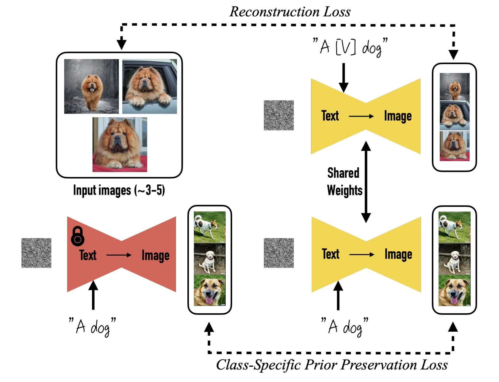
Identifier Token Selection Strategy
The effectiveness of DreamBooth hinges on selecting a subject token \( \mathbf {s} \) that is both learnable and semantically disentangled—meaning it has weak or no associations with existing concepts in the model’s pretraining distribution. If \( \mathbf {s} \) corresponds to a token that is already semantically rich (e.g., ”dog”, ”person”, ”red”), fine-tuning may corrupt unrelated concepts (semantic drift) or introduce identity leakage and reduced generative diversity. Conversely, if \( \mathbf {s} \) is rarely used during pretraining, the model is free to associate it entirely with the new subject.
Tokenizer Overview and Motivation
Like most modern text-to-image models, DreamBooth processes natural language prompts using a tokenizer—a component that maps raw text into a sequence of discrete token IDs. These IDs form the input to the model’s text encoder and are drawn from a fixed vocabulary that is constructed during pretraining on a large-scale corpus.
Rather than operating at the level of individual characters or entire words, modern tokenizers segment text into subword units—variable-length fragments like “red”, or “xxy5”. This subword decomposition strikes a practical balance between expressiveness and efficiency:
- It avoids the combinatorial explosion of full-word vocabularies, which would require millions of entries to cover rare terms, compound words, or typos.
- It reduces the sequence length relative to character-level tokenization, thereby improving model efficiency and allowing for longer contextual understanding.
- It ensures robustness: even unseen or rare words can still be represented using known fragments from the vocabulary.
The result is a compact, reusable, and expressive vocabulary that allows any input string—no matter how unusual—to be tokenized into a valid sequence of known token IDs. Each token ID is then mapped to a high-dimensional embedding vector via a static lookup table in the text encoder. These embeddings are passed through a Transformer-based architecture such as CLIP or T5 to produce contextualized representations used to condition the image generation process.
During image generation, particularly in diffusion-based architectures, the contextualized text embeddings influence visual outputs through dedicated cross-attention layers. These layers are embedded within the model’s U-Net architecture and act as an interface between the text encoder and the evolving image representation. Specifically, visual features derived from the noisy image (acting as attention queries) attend to the token-level embeddings (acting as keys and values), producing spatially localized responses. The result is a set of attention maps that modulate each region of the image according to its relevance to the corresponding text tokens.
This mechanism establishes a direct spatial-semantic correspondence: each region of the image learns to ”pay attention” to the appropriate linguistic concepts in the prompt. Such alignment is foundational for accurate text-to-image synthesis. In DreamBooth, this correspondence is further exploited during fine-tuning—where a rare identifier token is explicitly trained to control the appearance of a novel subject. The gradients from the cross-attention pathway reinforce the association between that token and spatial structures in the generated image, enabling the model to synthesize consistent and editable subject representations in response to prompt variations.
Rare Token Selection for Subject Identity Binding
DreamBooth performs subject personalization without altering the tokenizer or the text encoder. Instead of introducing new vocabulary, it repurposes an existing but underused token \( s_{\mbox{text}} \) from the tokenizer’s fixed vocabulary to symbolically represent a novel subject. This token’s embedding—denoted \( \vec {e}_s \in \mathbb {R}^d \)—is static, produced by the frozen text encoder, and interpreted only by the fine-tuned diffusion model (e.g., the U-Net).
The goal is to choose a token that behaves as a semantic blank slate: syntactically valid, visually neutral, and semantically unentangled. The U-Net is then trained to associate \( \vec {e}_s \) with the personalized subject appearance while leaving the text encoder entirely untouched. After training, prompts like "a sks dog in the snow" can reliably generate identity-consistent outputs in diverse contexts.
The rare-token selection strategy is general and applies to any text encoder–tokenizer pair. Below we outline a unified procedure applicable to both Imagen (using T5 with SentencePiece) and Stable Diffusion (using CLIP with Byte-Pair Encoding).
- 1.
- Enumerate the Tokenizer Vocabulary.
Each tokenizer defines a fixed mapping from token IDs to Unicode strings:- Imagen uses T5-XXL with a SentencePiece vocabulary of size 32,000.
- Stable Diffusion uses a CLIP-BPE tokenizer with approximately 49,000 tokens.
These mappings can be accessed via tokenizer APIs.
- 2.
- Identify Rare, Neutral Candidates.
The ideal token \( s_{\mbox{text}} \) is rare (low frequency) and lacks meaningful associations. For example:- In Imagen, token IDs in the range \[ \{5000, 5001, \ldots , 10000\} \] are empirically found to be infrequent in the training corpus and often decode to short, nonsensical strings like sks, qxl, or zqv.
- In Stable Diffusion, naive strings like sks may be split into multiple tokens unless formatted with brackets (e.g., [sks]) to ensure they are tokenized as a single unit.
- 3.
- Filter Structurally Valid Tokens.
Candidate tokens must satisfy the following constraints:- Decodability: The token maps to a valid, printable Unicode string.
- Length: Ideally 1–3 characters or a compact glyph.
- Token integrity: It must remain a single token after tokenization.
- Semantic neutrality: It should not resemble common words, brand names, or known entities.
Once a valid token is chosen, it is held fixed and used in all subject-specific prompts during DreamBooth finetuning. The text encoder produces a static embedding \( \vec {e}_s \), while only the U-Net learns to interpret it as the visual identity of the subject. This setup supports prompt compositionality, enabling queries like:
- "a watercolor painting of a sks vase in a spaceship"
- "a sks dog painted by Van Gogh"
- "a sks backpack on the Moon"
In summary, the reuse of rare tokens provides an elegant, encoder-compatible mechanism for subject binding. By leveraging frozen embeddings with minimal prior entanglement, DreamBooth enables high-fidelity personalization while preserving the expressive power of the original generative model.
In the following, we describe how this token selection integrates into the full DreamBooth training procedure, including loss functions that ensure both precise subject encoding and generalization to new contexts.
Training Objective and Prior Preservation Once a rare identifier token \( s_{\mbox{text}} \) has been selected and inserted into structured prompts, DreamBooth fine-tunes the pretrained text-to-image model to associate the subject with its corresponding static embedding \( \vec {e}_s \). Training follows the denoising diffusion paradigm, augmented with a regularization term that preserves the model’s generative flexibility.
Main Loss: Denoising Objective Let \( \{x_1, x_2, \dots , x_n\} \) denote a small subject dataset, and let each image \( x_i \) be paired with a prompt \( y_i = \texttt{"a photo of a } s_{\mbox{text}} \texttt{ class"} \). The fine-tuning process proceeds as follows:
- 1.
- Encode each image \( x_i \) using the frozen image encoder:
- For LDMs: obtain latent representation \( \vec {z}_i = \mbox{Enc}(x_i) \).
- For pixel-space models (e.g., Imagen): use \( \vec {z}_i = x_i \).
- 2.
- Sample a timestep \( t \sim \mathcal {U}(\{1, \dots , T\}) \) and corrupt the input: \[ \vec {z}_{i,t} = \sqrt {\bar {\alpha }_t} \vec {z}_i + \sqrt {1 - \bar {\alpha }_t} \, \vec {\epsilon }, \quad \vec {\epsilon } \sim \mathcal {N}(0, \vec {I}). \]
- 3.
- Encode the prompt \( y_i \) using the frozen text encoder to obtain embeddings \( \vec {E}_i \), where \( \vec {e}_s \in \vec {E}_i \) denotes the token embedding of \( s_{\mbox{text}} \).
- 4.
- Input \( (\vec {z}_{i,t}, t, \vec {E}_i) \) into the U-Net and predict the noise: \[ \hat {\vec {\epsilon }} = \mbox{U-Net}(\vec {z}_{i,t}, t, \vec {E}_i). \]
- 5.
- Minimize the reconstruction loss: \[ \mathcal {L}_{\mbox{recon}} = \left \| \hat {\vec {\epsilon }} - \vec {\epsilon } \right \|_2^2. \]
During this process, only the U-Net parameters (and optionally its cross-attention layers) are updated. The tokenizer, text encoder, and VAE remain frozen.
Preventing Overfitting: Prior Preservation Loss Since DreamBooth typically trains on as few as 3–5 images, it is prone to overfitting—resulting in memorized poses, lighting, or background, and catastrophic forgetting of class diversity. To mitigate this, DreamBooth introduces a prior preservation loss that encourages the model to retain generative variability across the subject’s class.
This is implemented by mixing in a batch of generic class instances:
- For each batch, sample additional images \( \{x^{\mbox{prior}}_j\} \) with prompts like "a photo of a dog", omitting the identifier token.
- Apply the same forward corruption process and compute the corresponding loss: \[ \mathcal {L}_{\mbox{prior}} = \left \| \hat {\vec {\epsilon }}_{\mbox{prior}} - \vec {\epsilon } \right \|_2^2. \]
The final training objective becomes: \[ \mathcal {L}_{\mbox{total}} = \mathcal {L}_{\mbox{recon}} + \lambda \cdot \mathcal {L}_{\mbox{prior}}, \] where \( \lambda \in \mathbb {R}_+ \) controls the strength of prior preservation (typically \( \lambda = 1.0 \)).
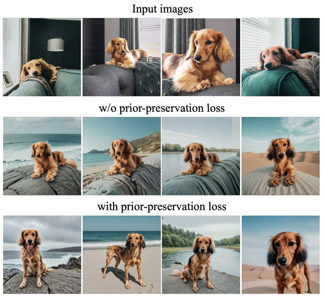
Effect and Interpretation The prior-preservation term acts as a semantic constraint: it encourages the model to treat the identifier \( s_{\mbox{text}} \) as a distinct instance within a broader class, rather than as a class replacement. This enables:
- Preserves the model’s ability to generate diverse class-consistent outputs (e.g., dogs in snow, with accessories, or in unusual settings).
- Enables identity-grounded generation in novel contexts—e.g., "a sks dog in the desert", "a sks dog jumping over a fence", or "a sks dog wearing sunglasses".
This balance between memorization and generalization is critical for subject-driven generation to remain flexible and compositional. In the following, we explore how DreamBooth leverages this setup to enable high-fidelity identity transfer across scenes, styles, and visual manipulations.
Subject-Driven Generation in New Contexts Once DreamBooth has successfully fine-tuned the model to bind a unique token \(\mathbf {s}\) to a subject identity, it can be used to generate photorealistic or stylized images of that subject in a wide range of scenarios. Unlike traditional overfitted fine-tuning techniques, DreamBooth supports rich recontextualization—the subject can be rendered in scenes it was never observed in, under varying lighting conditions, poses, styles, and semantic compositions.
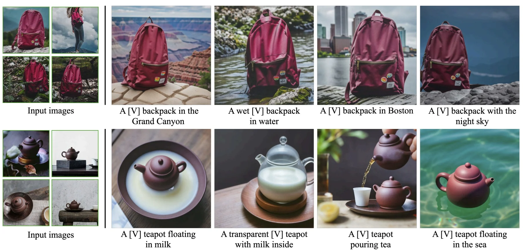
This capability is made possible by the model’s retained understanding of the subject’s class (e.g., “teapot”, “dog”)—due to the prior preservation loss—and the flexibility to modify the subject’s expression, pose, or style through text prompts:
- \a sks dog crying", \a sks dog sleeping", \a sks dog smiling" — expression manipulation
- \a Van Gogh painting of a sks dog" — style transfer
- \a sks dog with wings", \a sks dog in the style of a sculpture" — compositional attributes
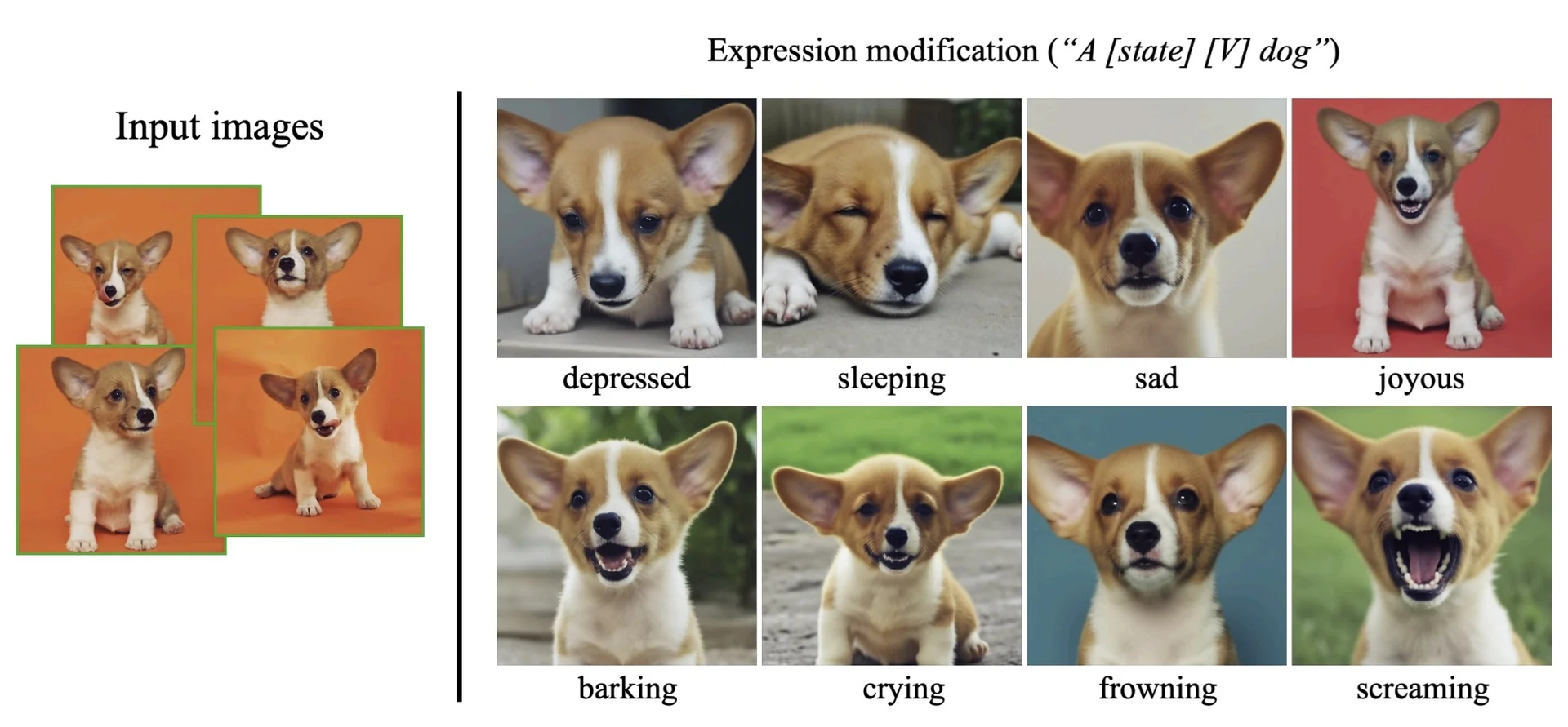
DreamBooth also supports zero-shot outfitting and attribute additions. Guided by prompt text, the model composes realistic physical interactions between the subject and newly specified objects, outfits, or environments.
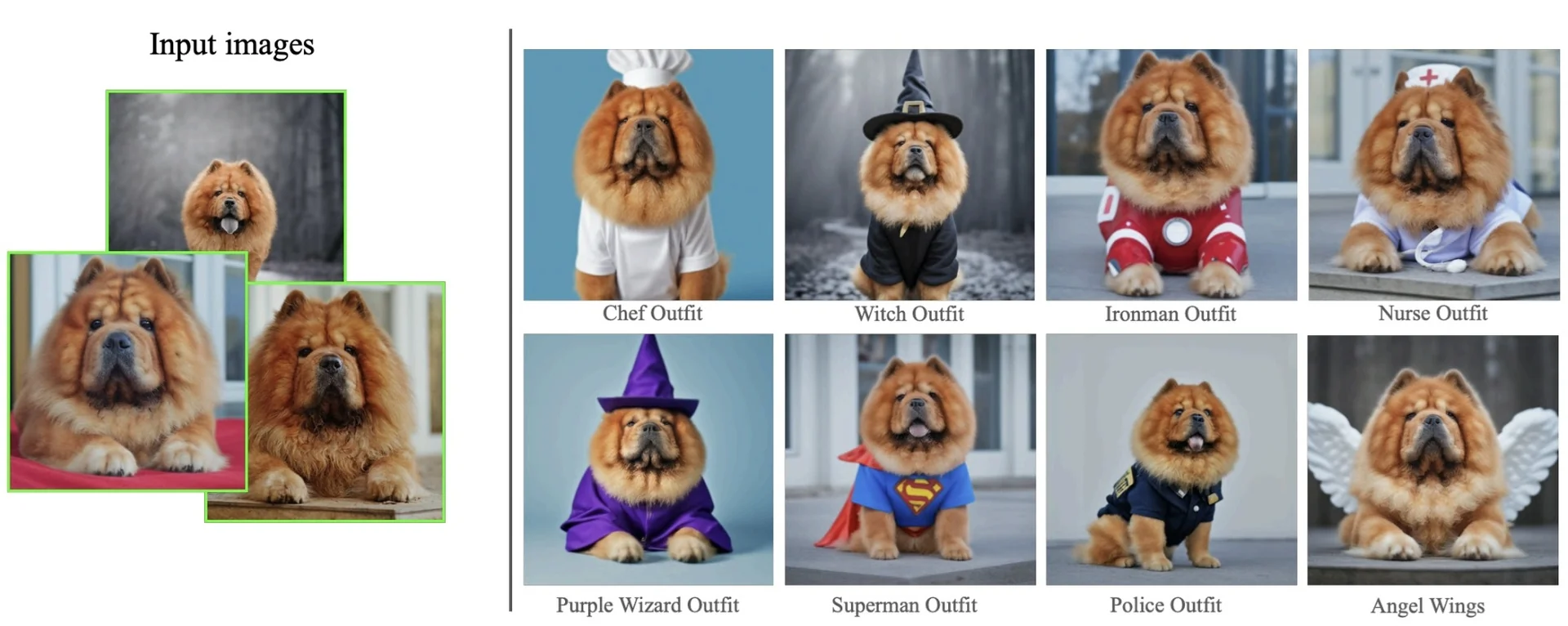
By decoupling the subject embedding \(\mathbf {s}\) from specific backgrounds, poses, and lighting, DreamBooth enables flexible recombination with diverse prompts. This supports high-fidelity identity preservation across scenes, compositions, and artistic styles—unlocking broad applications in personalized content creation, from digital avatars and branded photography to stylized storytelling.
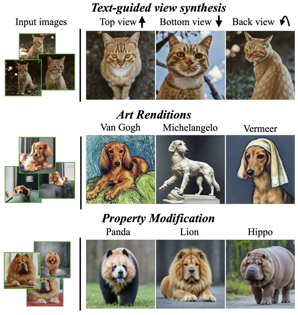
These capabilities highlight DreamBooth’s ability to interpolate both pose and rendering domain. Viewpoint shifts and stylistic alterations—unseen in the training images—are synthesized faithfully while retaining fine-grained subject detail. This extends the model’s generative capacity far beyond memorization.
Nonetheless, DreamBooth is not without limitations. Some failure modes arise in rare contexts, entangled prompts, or when the model overfits to specific image details.
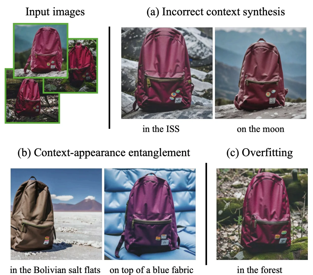
While DreamBooth achieves impressive subject fidelity, it often struggles with precise compositional control. Issues such as background entanglement, pose collapse, or implausible scene generation persist—especially when attempting to render the subject in unfamiliar contexts. Prompt-to-Prompt [226] addressed some of these shortcomings by manipulating cross-attention maps to steer how specific words influence spatial regions of the image. However, its control remains fundamentally implicit—limited to prompt structure and lacking direct spatial supervision.
This motivates a shift toward explicit conditioning: instead of relying solely on text, can we guide generation using structured visual signals such as edge maps, depth fields, or pose skeletons? ControlNet provides a powerful answer to this question. By injecting auxiliary control encoders into the diffusion backbone, ControlNet enables fine-grained spatial, geometric, and semantic modulation of the generation process—dramatically improving compositional accuracy and unlocking new applications in image editing, synthesis, and personalized rendering.
In the following, we examine the architecture, training procedure, and capabilities of ControlNet, highlighting how it can be used independently or in conjunction with methods like DreamBooth to enhance controllability and visual grounding.
Enrichment 20.11.8: ControlNet – Structured Conditioning for Diffusion Models
Motivation and Background Despite the remarkable success of prompt-based diffusion models in generating photorealistic and semantically coherent images, they offer only coarse-grained control over the structure and layout of the output. Natural language prompts—such as “a person riding a bicycle near the ocean”—are inherently ambiguous in spatial and geometric terms. As a result, generated scenes may omit critical elements, produce anatomically implausible poses, or fail to match user intent in fine-grained ways.
This limitation stems from the fact that text alone cannot precisely encode spatial or visual structure. Concepts such as object pose, layout, depth, or boundaries are difficult to express in natural language and even harder for the model to ground consistently. Methods like DreamBooth [554] improve subject identity preservation, and techniques such as Prompt-to-Prompt [226] allow for localized prompt manipulation via attention maps—but both approaches rely solely on textual cues and offer no mechanism for incorporating structured visual guidance.
To address these challenges, ControlNet [794] introduces a principled architectural extension to diffusion models that enables conditioning on external visual signals. These conditioning inputs—such as edge maps, human poses, depth estimates, scribbles, or segmentation masks—serve as explicit spatial priors, providing the model with structured cues that text alone cannot supply. For example, a depth map can enforce perspective geometry in a 3D interior scene, while a pose skeleton can define limb orientation and articulation in human generation tasks.
ControlNet thus empowers users to inject high-level semantic intent through text while simultaneously guiding low-level spatial structure via visual hints—bridging the gap between language-driven generation and precise, user-defined control over image composition.
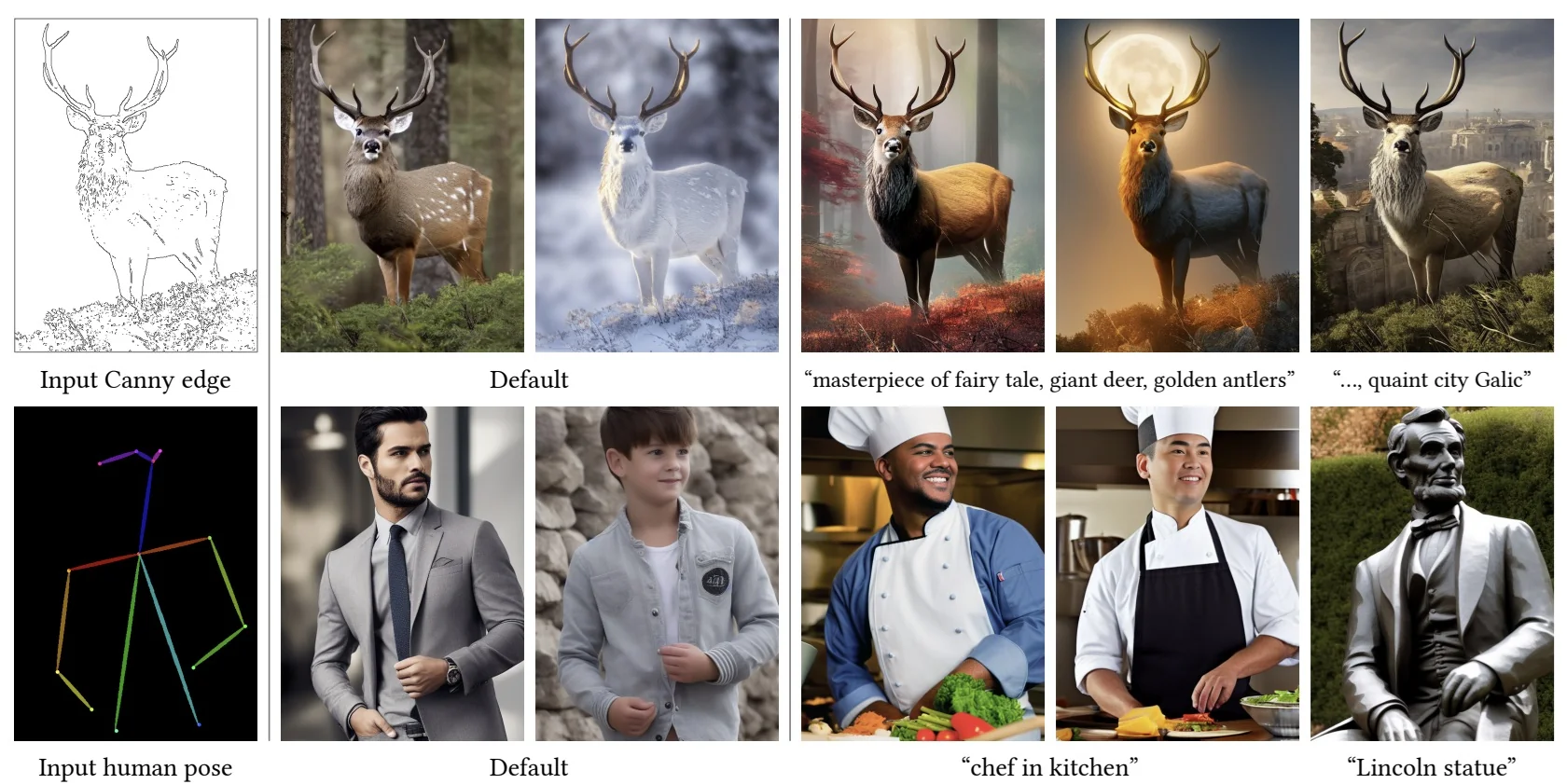
This capability is especially important in domains where spatial layout matters—such as:
- Pose-to-image generation (e.g., rendering a person performing a specific action).
- Edge-to-photo synthesis (e.g., recreating objects from sketches).
- Semantic-to-scene mapping (e.g., transforming segmentation maps into photorealistic scenes).
By introducing minimal architectural overhead and preserving the core capabilities of the base diffusion model, ControlNet bridges the gap between prompt conditioning and structured visual control. In the following, we will examine its design, training procedure, and practical benefits.
Block Injection and Architectural Motivation ControlNet augments large pretrained text-to-image diffusion models—such as Stable Diffusion—by introducing a trainable conditional branch designed to interpret external structural cues (e.g., edge maps, depth, pose, segmentation) while preserving the integrity of the base model. These external cues are encoded as condition maps \( c \in \mathbb {R}^{H \times W \times C} \), and are used in conjunction with the usual text prompt \( y \), forming a dual conditioning scheme:
- The text prompt is tokenized and encoded by a frozen text encoder (e.g., CLIP), producing embeddings that are injected into the U-Net via cross-attention layers.
- The condition map is passed through a dedicated encoder, whose outputs are injected into a trainable replica of the U-Net blocks, spatially guiding generation at each resolution.
ControlNet’s integration with large-scale pretrained diffusion models represents a significant architectural innovation. Rather than retraining a diffusion model from scratch—a process that would require massive datasets like LAION-5B [574], which are tens of thousands of times larger than typical condition-specific datasets—ControlNet employs a far more efficient strategy.
It locks the parameters of a production-ready model, such as Stable Diffusion [548], thereby preserving its high-fidelity generation capabilities acquired through training on billions of image–text pairs. Simultaneously, it introduces a trainable replica of each internal block in the U-Net backbone. These replicas allow the model to adapt to new forms of spatial or structural conditioning (e.g., edges, depth, pose) without disrupting the semantics encoded in the original weights. This approach avoids overfitting and catastrophic forgetting—common pitfalls in low-data fine-tuning scenarios [358].
A key architectural mechanism enabling this safe dual-path design is the use of zero convolutions [794]. These are \(1 \times 1\) convolution layers whose weights and biases are initialized to zero. As a result, the conditional branches contribute nothing at the beginning of training, ensuring that the pretrained activations remain untouched. Gradually, as gradients update these layers, the conditional signal is introduced in a controlled, non-disruptive manner. This guarantees a stable warm-start and protects the pretrained backbone from the destabilizing effects of random gradient noise early in training.
Enrichment 20.11.8.1: ControlNet Architecture
Injecting Spatial Conditioning into Frozen Networks Large-scale pretrained models such as the U-Net used in Stable Diffusion exhibit remarkable generative capabilities, especially when guided by text prompts. However, their reliance on linguistic conditioning alone limits their ability to follow spatial instructions—such as replicating object pose, structural contours, or depth information—especially in tasks requiring precise layout control. This gap motivates the development of ControlNet, a framework that injects spatial condition maps into the intermediate layers of a frozen pretrained diffusion model, enabling fine-grained control while preserving generative quality.
Let \( \mathcal {F}(\cdot ; \Theta ) \) denote a frozen network block, where a block refers to a modular transformation unit such as a residual block or Transformer layer. Given an input feature map \( x \in \mathbb {R}^{H \times W \times C} \), the block produces an output feature map \( y = \mathcal {F}(x; \Theta ) \). These feature maps encode semantically and spatially rich representations used progressively in denoising-based generation.
ControlNet Architectural Design To augment the network with conditioning, ControlNet associates each frozen block \( \mathcal {F}(\cdot ; \Theta ) \) with a trainable replica \( \mathcal {F}(\cdot ; \Theta _c) \). This replica processes both the original feature map \( x \) and an external condition map \( c \in \mathbb {R}^{H \times W \times C} \), such as a Canny edge image, depth map, or human pose keypoints. The condition map is transformed into a residual signal through a pair of zero-initialized \( 1 \times 1 \) convolution layers:
\begin {equation} y_c = \mathcal {F}(x; \Theta ) + \mathcal {Z} \left ( \mathcal {F}\left (x + \mathcal {Z}(c; \Theta _{z1}); \Theta _c \right ); \Theta _{z2} \right ) \end {equation}
Here, \( \mathcal {Z}(\cdot ; \Theta _{z1}) \) injects the condition into the input space of the trainable replica, while \( \mathcal {Z}(\cdot ; \Theta _{z2}) \) modulates the output. Both zero convolutions are initialized such that their weights and biases are exactly zero, ensuring that the condition path introduces no change at the start of training.
Motivation for Additive Injection: Why Not Inject \( c \) Directly? A seemingly natural idea would be to inject the condition map \( c \) directly into the layers of the frozen U-Net—via concatenation, addition, or feature fusion. However, this naive approach often results in degraded output quality. The pretrained model encodes subtle statistical priors learned from billions of image-text pairs. Tampering with these internal representations, especially with limited data and abrupt injections, may cause:
- Catastrophic Forgetting: Directly modifying the feature flow may cause the model to forget its generative priors, reducing sample diversity and fidelity.
- Semantic Drift: Uncontrolled condition injection can skew the model’s internal representations, leading to mismatches between prompts and outputs.
- Training Instability: The injection introduces mismatched signals, leading to noisy gradients and divergence during optimization.
ControlNet avoids these pitfalls by enforcing architectural separation: the condition map \( c \) flows through a parallel, trainable branch that computes residual corrections to the output of the frozen U-Net. These corrections are injected additively via zero-initialized \( 1 \times 1 \) convolutions, ensuring that pretrained knowledge remains unperturbed at the start of training. This design enables progressive alignment, where the residuals only modify the output when helpful.
- \( \mathcal {F}(x; \Theta ) \): The original U-Net block with frozen weights \( \Theta \), trained on large-scale image-text data and reused without modification.
- \( \mathcal {F}(x'; \Theta _c) \): A trainable replica of the frozen block, receiving a perturbed input \( x' = x + \mathcal {Z}(c; \Theta _{z1}) \), where \( \mathcal {Z} \) is a zero-initialized convolution.
- \( \mathcal {Z}(\cdot ; \Theta _{z1}) \), \( \mathcal {Z}(\cdot ; \Theta _{z2}) \): Zero-initialized \(1 \times 1\) convolutions used at the input and output of the trainable path, regulating the influence of the conditional signal.
How Can the Output Change If the U-Net Is Frozen? And Why Is Denoising Still Valid? Freezing the U-Net implies that its output remains unchanged—but ControlNet introduces a trainable parallel path that circumvents this limitation. At each U-Net block, a residual branch is appended and fused with the frozen output via zero-initialized \( 1 \times 1 \) convolutions:
\begin {equation} y_c = \mathcal {F}(x; \Theta ) + \mathcal {Z}_2 \left ( \mathcal {F}(x + \mathcal {Z}_1(c; \Theta _{z1}); \Theta _c); \Theta _{z2} \right ) \end {equation}
Initially, both \( \mathcal {Z}_1 \) and \( \mathcal {Z}_2 \) are zero-initialized, making \( y_c = \mathcal {F}(x; \Theta ) \)—identical to the pretrained model. This ensures a safe warm start that avoids destabilization.
Although the residual branches in ControlNet are initialized with zero convolution layers—meaning all weights \( W \) and biases \( B \) are set to zero at the beginning of training—they remain fully trainable. The forward pass of such a layer for an input feature map \( I \in \mathbb {R}^{H \times W \times C} \) is defined as:
\begin {equation} Z(I; \{W, B\})_{p,i} = B_i + \sum _j I_{p,j} W_{i,j} \end {equation}
At initialization, since \( W = 0 \) and \( B = 0 \), the output is zero. However, the gradients behave as follows (where \( \frac {\partial \mathcal {L}}{\partial Z} \) denotes the upstream gradient):
\begin {align} \frac {\partial Z(I; \{W, B\})_{p,i}}{\partial B_i} &= 1 \\ \frac {\partial Z(I; \{W, B\})_{p,i}}{\partial I_{p,i}} &= \sum _j W_{i,j} = 0 \\ \frac {\partial Z(I; \{W, B\})_{p,i}}{\partial W_{i,j}} &= I_{p,j} \end {align}
We see that while the gradient with respect to the input \( I \) is zero initially (due to \( W = 0 \)), the gradients with respect to the bias \( B \) and the weights \( W \) are non-zero as long as the input feature \( I \) itself is non-zero—which is always the case in practice, since \( I \) encodes the image or conditioning information.
This mechanism ensures that the first gradient descent step will update the weights to non-zero values. For example, assuming a non-zero learning rate \( \beta _{\mbox{lr}} \) and loss gradient \( \partial \mathcal {L} / \partial Z \neq 0 \), the weight update becomes:
\begin {equation} W^* = W - \beta _{\mbox{lr}} \cdot \left ( \frac {\partial \mathcal {L}}{\partial Z} \odot \frac {\partial Z}{\partial W} \right ) \end {equation}
where \( \odot \) denotes the Hadamard (elementwise) product. After this step, the weight matrix \( W^* \) becomes non-zero, and the layer begins to propagate gradients to its input as well:
\begin {equation} \frac {\partial Z(I; \{W^*, B\})_{p,i}}{\partial I_{p,j}} = \sum _j W^*_{i,j} \neq 0 \end {equation}
Training Objective ControlNet is fine-tuned using the standard diffusion loss, augmented to include both spatial and textual conditioning. This objective trains the model to predict the noise added to a latent image representation at a given timestep, while also respecting high-level textual and low-level spatial guidance.
Each training sample includes:
- \( z_0 \): Clean latent representation, encoded from a \(512 \times 512\) image using a frozen VQ-GAN encoder [149, 548].
- \( \epsilon \sim \mathcal {N}(0, I) \): Gaussian noise.
- \( t \in \{1, \ldots , T\} \): Diffusion timestep.
- \( z_t = \sqrt {\bar {\alpha }_t} z_0 + \sqrt {1 - \bar {\alpha }_t} \, \epsilon \): Noised latent using cumulative schedule \(\bar {\alpha }_t\).
- \( c_t \): Text embedding from a frozen encoder (e.g., CLIP) [512]. During training, 50% of prompts are replaced with empty strings to promote reliance on spatial inputs [794].
- \( c_i \): Spatial condition image (e.g., pose, depth, edges) deterministically derived from \(z_0\).
- \( c_f = \mathcal {E}_{\mbox{cond}}(c_i) \): Feature map from a shallow encoder \(\mathcal {E}_{\mbox{cond}}\), aligned to U-Net resolution.
The loss function is: \begin {equation} \mathcal {L}_{\mbox{ControlNet}} = \mathbb {E}_{z_0, t, \epsilon , c_t, c_f} \left [ \left \| \epsilon - \epsilon _\theta (z_t, t, c_t, c_f) \right \|_2^2 \right ] \label {eq:controlnet_loss} \end {equation}
Why ControlNet Preserves Denoising Capability ControlNet extends pretrained diffusion models with spatial guidance while preserving their original denoising behavior. This is achieved through a design that carefully introduces conditional influence without interfering with the U-Net’s pretrained functionality.
At the heart of the diffusion process lies a U-Net trained to predict noise across billions of images [548]. In ControlNet, this U-Net is left entirely frozen during training [794], meaning it continues to perform the same denoising task it was originally optimized for. The key innovation lies in how ControlNet introduces its new functionality: by attaching a parallel, trainable branch whose outputs are added to the internal feature maps of the frozen U-Net at each resolution [794].
Initially, this residual branch is non-functional. All connecting \(1 \times 1\) convolution layers are zero-initialized—both weights and biases—which guarantees that the trainable path contributes no signal at the beginning. Thus, the model’s forward pass and denoising predictions are initially identical to the pretrained backbone. Crucially, despite being inactive at first, these zero-initialized layers admit nonzero gradients with respect to both their weights and biases. As long as the input condition maps contain nonzero values (which they typically do), gradient descent immediately begins to train the ControlNet branch—starting from a neutral baseline and gradually learning how to steer the generation process.
This training strategy ensures that conditional guidance is introduced in a progressive and reversible way. Because the U-Net remains frozen, the core noise prediction function is never corrupted. Instead, ControlNet learns to produce residual corrections that refine the denoising trajectory in a way that respects both the diffusion objective and the spatial constraints imposed by the conditioning input. The result is a denoising model that continues to predict valid noise estimates, now informed by an auxiliary signal such as an edge map or pose skeleton.
In essence, ControlNet does not replace the original model’s logic—it learns to nudge it. The trainable branch aligns the latent noise prediction with external guidance, but the primary computation and structure of the denoising process remain governed by the fixed U-Net. This preserves the quality, stability, and generalization of the pretrained model while enabling precise spatial control.
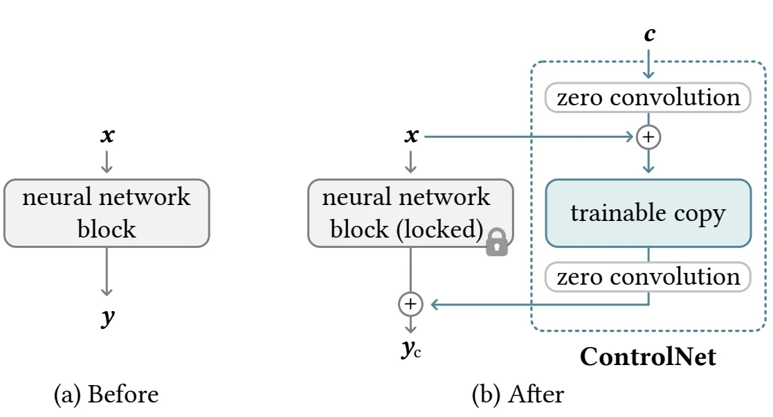
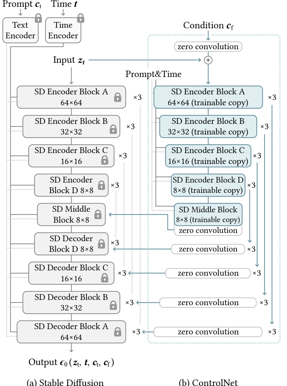
We now continue focusing on ControlNet’s training dynamics, sudden convergence behavior, and the role of Classifier-Free Guidance (CFG):
Enrichment 20.11.8.2: Training Behavior and Sudden Convergence
A key strength of ControlNet’s architectural design lies in its training stability. Thanks to the zero-initialized convolution layers that bridge the frozen and trainable branches, the model behaves identically to the original Stable Diffusion at initialization. This ensures that the first forward passes produce coherent images, even before any optimization occurs.
As training progresses, gradients propagate through the zero convolutions and update the trainable ControlNet branches. Initially, these branches exert no influence on the output. However, within a few thousand training steps, a phenomenon referred to as sudden convergence emerges: the ControlNet rapidly learns to inject the condition map into the generation process in a semantically meaningful way.
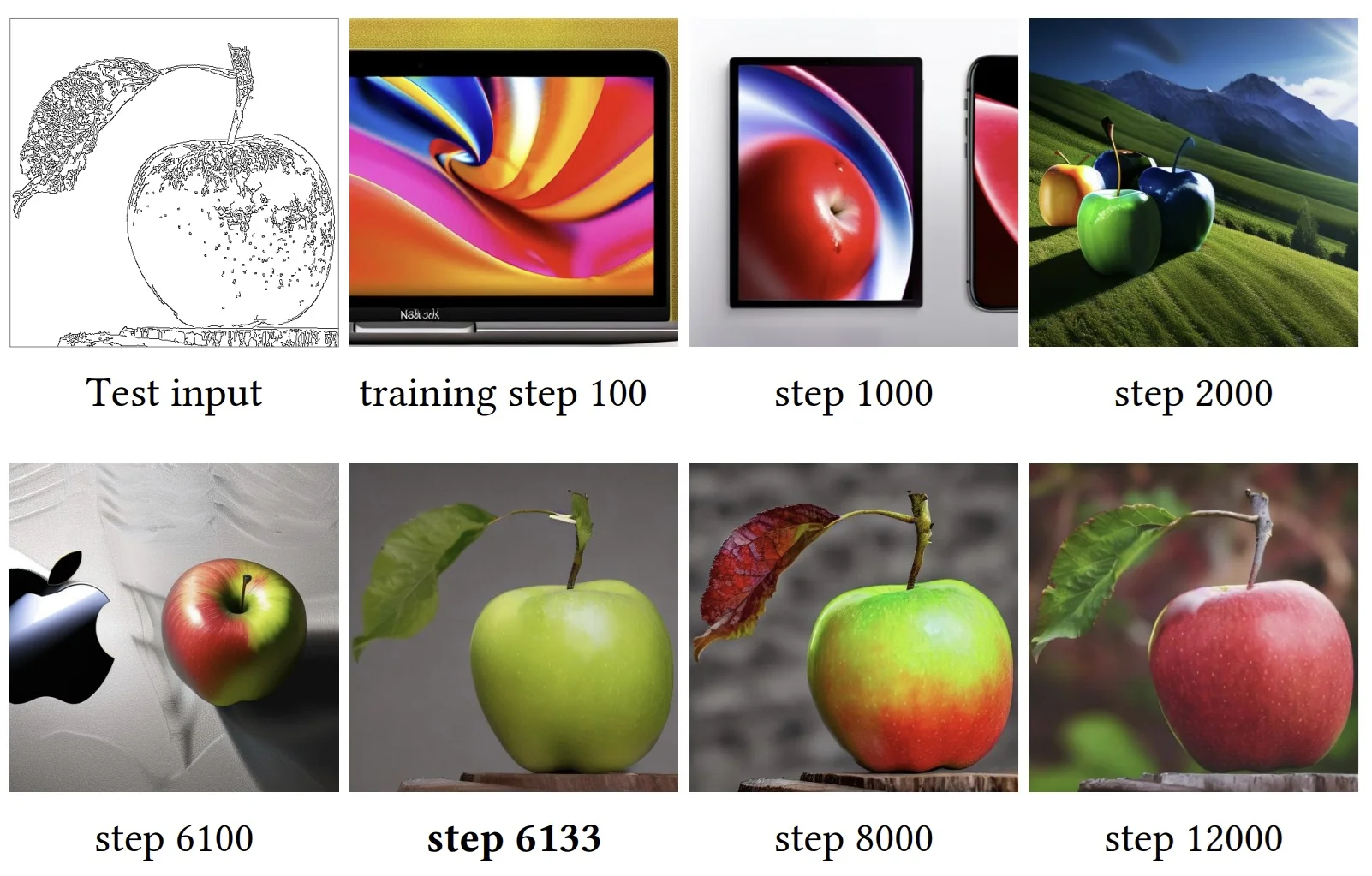
This behavior reflects the progressive unfreezing of the control pathway: the zero-initialized convolutions learn how to linearly transform the conditioned features to guide generation, while the trainable U-Net blocks learn to interpret the condition map. Throughout this process, the frozen base model remains intact, continuing to produce high-quality visual content.
Classifier-Free Guidance and Resolution-Aware Weighting ControlNet enhances the capabilities of diffusion models by integrating Classifier-Free Guidance (CFG) [233], a technique that balances adherence to conditioning inputs (like text prompts) with the diversity and realism of generated images. Additionally, ControlNet introduces a novel refinement: Classifier-Free Guidance Resolution Weighting (CFG-RW), which dynamically adjusts guidance strength across different spatial resolutions to optimize both semantic alignment and visual fidelity.
Classifier-Free Guidance (CFG) that we’ve covered in Enrichment 20.9.3 operates by training the diffusion model to handle both conditional and unconditional scenarios. During training, the conditioning input (e.g., text prompt \( y \)) is randomly omitted in a subset of training instances (commonly 50%), compelling the model to learn representations that are robust to the absence of explicit conditions. At inference, the model combines the conditional prediction \( \epsilon _{\mbox{cond}} \) and the unconditional prediction \( \epsilon _{\mbox{uncond}} \) using a guidance scale \( \lambda \):
\[ \epsilon _{\mbox{CFG}} = \epsilon _{\mbox{uncond}} +\lambda \cdot (\epsilon _{\mbox{cond}} - \epsilon _{\mbox{uncond}}) \]
This formulation allows users to modulate the influence of the conditioning input, with higher values of \( \lambda \) enforcing stronger adherence to the condition, potentially at the cost of image diversity.
Resolution-Aware Weighting (CFG-RW) Resolution-Aware Weighting (CFG-RW) is a critical mechanism that enables effective conditioning in ControlNet by adapting the strength of the guidance signal to the spatial resolution of each layer in the U-Net. Rather than applying a uniform scale to all residual injections, CFG-RW introduces a dynamic scheme:
\[ w_i = \frac {64}{h_i} \]
where \( w_i \) is the guidance weight applied at a layer with spatial height \( h_i \). This design is grounded in the hierarchical nature of the U-Net and the dynamics of the denoising process in diffusion models. The key to preserving the base model’s generative capabilities lies in regulating the influence of these residuals according to resolution.
- Low-resolution layers (e.g., \(8 \times 8\), \(16 \times 16\)) are responsible for encoding global structure—object positions, shapes, and scene layout. These layers benefit from strong guidance, as alignment at this scale is critical for conditioning to take effect. Hence, CFG-RW assigns large weights (e.g., \(w_i = 8\) for \(h_i = 8\)) to amplify the control signal.
- High-resolution layers (e.g., \(32 \times 32\), \(64 \times 64\)) refine textures, edges, and fine detail. Here, excessive guidance can distort or overwrite the pretrained model’s realistic priors. Small weights (e.g., \(w_i = 1\) for \(h_i = 64\)) preserve freedom for the U-Net to leverage its learned generative capacity.
Why It Works Diffusion models denoise from coarse to fine: early steps shape global semantics, while later ones refine textures. ControlNet injects conditioning through residuals at every U-Net layer, but applying a uniform strength across resolutions introduces issues:
- Too weak at low resolutions: Structural guidance is underutilized, leading to semantic drift.
- Too strong at high resolutions: Fine details are over-constrained, reducing realism.
Resolution-Aware Weighting (CFG-RW) resolves this by scaling the residual strength inversely with spatial resolution. This ensures: stronger guidance for layers encoding coarse structure, and softer influence where detail synthesis must remain flexible. Because the base U-Net is frozen, this modulation gently steers the generative process without destabilizing pretrained behavior.
Training Intuition With CFG-RW ControlNet is trained on a small paired dataset \((x, y)\), where \(x\) is the conditioning input and \(y\) the target image. The denoising objective remains unchanged, and only the ControlNet branch is updated. Residuals start with zero-initialized weights, ensuring that early training mimics the original model. As gradients accumulate, residuals learn to inject useful control, progressively modulated by CFG-RW to balance structure and detail. This setup enables stable finetuning while preserving generative fidelity.
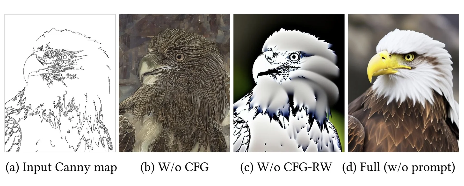
In summary, the integration of CFG and the introduction of CFG-RW in ControlNet provide a nuanced mechanism for balancing condition adherence and image realism. By dynamically adjusting guidance strength across resolutions, ControlNet achieves high-quality, semantically aligned image generation, even when conditioned on complex inputs like edge maps or depth maps. This advancement underscores ControlNet’s robustness and versatility in controllable image synthesis. In the next part, we explore the limitations of ControlNet, motivating us towards following works.
Limitations of ControlNet and the Need for Semantic Conditioning ControlNet represents a major advance in controllable image synthesis. By introducing condition maps—such as Canny edges, human poses, or depth estimates—into a frozen diffusion model, it enables users to steer image generation with fine-grained structural constraints. However, it is important to emphasize a subtle but critical limitation: although ControlNet can be trained on full images, it cannot directly accept them as conditioning inputs. Instead, the image must be converted into a structural map—such as an edge sketch or depth projection—via a separate preprocessing pipeline.
This design choice is not arbitrary. The control branch in ControlNet is injected as residual guidance into a frozen U-Net, where each layer encodes spatially aligned features at different resolutions. To avoid interfering with the pretrained backbone, the injected condition must be spatially structured and semantically simple—matching the inductive biases of the U-Net. Raw RGB images are too entangled: they mix high-level semantics with textures, lighting, and style cues that do not map cleanly onto the diffusion model’s feature hierarchy. Structural maps, by contrast, are sparse, modality-aligned inputs that can guide early-stage generation without disrupting fine detail synthesis.
As a result, even when the training dataset contains full images, ControlNet learns to rely on their preprocessed structural representations. These projections are useful but inherently limited, as they discard much of the image’s global context.
Several limitations arise from this design:
- Brittle and domain-specific. The quality of condition maps depends on external models (e.g., edge detectors or depth estimators), which may fail on atypical, occluded, or stylized inputs.
- Workflow friction. Generating these maps adds overhead to the user pipeline, breaking the simplicity of prompting with raw images.
- Information bottleneck. Much of the source image’s richness—style, mood, identity—is lost when projecting it into a sparse or low-resolution structural format.
Lack of Semantic Awareness The core limitation of ControlNet is its inability to condition on high-level visual semantics:
- It cannot preserve or replicate an individual’s identity, since structure alone is insufficient to describe fine facial or bodily characteristics.
- It does not capture or transfer artistic style, which depends on texture, color, and abstraction—not just shape or layout.
- It cannot convey emotional tone or scene context, which emerge from the global gestalt of an image rather than any explicit structural map.
Limited Compositionality and Scalability While ControlNet supports combining multiple condition maps (e.g., pose + depth), doing so often requires separate parallel branches, each tied to its own preprocessor and parameter set. This introduces:
- Architectural complexity. Adding more conditions increases VRAM usage and inference latency.
- Signal conflict. Structural conditions may provide conflicting guidance (e.g., pose suggests one layout, depth another), requiring manual resolution or custom weighting schemes.
These shortcomings underscore a key insight: ControlNet excels at where things go, but not at what they are. It anchors generation to spatial constraints, but ignores the high-level visual semantics that define identity, style, and intent.
This motivates a new class of conditioning methods—those that allow users to guide generation using images themselves as prompts. Rather than reducing an image to its skeletal structure, these approaches aim to preserve and transfer the holistic content, mood, and semantics encoded in the image. One such solution, which we present next, is the IP-Adapter framework: a modular design for injecting semantic image features into pretrained diffusion models without retraining or disrupting text conditioning.
Enrichment 20.11.9: IP-Adapter — Semantic Image Prompting for DMs
Motivation and Background Text-to-image diffusion models, such as Stable Diffusion, have revolutionized the field of generative AI by producing high-fidelity images from textual descriptions. However, guiding these models to generate images that precisely match user intent can be challenging. Crafting effective prompts often involves intricate prompt engineering, where users must carefully phrase their descriptions to elicit specific visual attributes. Moreover, text alone may fall short in conveying complex scenes, abstract concepts, or nuanced styles, limiting the creative control available to users.
To address these limitations, incorporating image prompts emerges as a compelling alternative. The adage “a picture is worth a thousand words” aptly captures the value of visual cues in conveying detailed information. Image prompts can encapsulate intricate styles, specific identities, or subtle emotional tones that might be difficult to articulate through text alone. Early methods, such as DALL·E 2, introduced image prompting capabilities but often required extensive fine-tuning of the entire model, which was computationally intensive and risked compromising the model’s original text-to-image performance. More recent approaches, like ControlNet, have provided structural control by conditioning on explicit visual features such as edges, depth maps, or poses. However, these methods rely on external preprocessing and lack inherent semantic understanding of high-level concepts, and often fine-grained features we want to retain in the generation process.
Introducing IP-Adapter: A Lightweight and Compatible Solution IP-Adapter [755] provides a plug-and-play mechanism for adding image prompt conditioning to pretrained text-to-image diffusion models—without any modification to the U-Net itself. Instead of forcing image and text information through the same cross-attention heads—heads that were originally trained exclusively on text—the adapter introduces a decoupled pathway: one cross-attention block for the text prompt (frozen), and one for the image prompt (trainable), both attending to the same latent query features.
Imagine two expert interpreters:
- The original, frozen attention module is a linguist—precisely trained to interpret prompts like “a smiling woman in a red dress.”
- The adapter is an art critic—skilled in extracting pose, style, texture, and fine-grained visual cues from a reference image.
Both receive the same Query—a partial image undergoing denoising—and offer distinct “translations” (attention outputs). The fusion of these two outputs forms a single signal that guides the next denoising step.
Why IP-Adapter Works Without Compromising the Base Model
1. Image Guidance via Decoupled Cross-Attention in U-Net Blocks The U-Net architecture used in diffusion models contains multiple cross-attention blocks distributed along its downsampling and upsampling paths. Each of these blocks incorporates text conditioning by computing attention outputs using queries \( Q = Z W_q \), keys \( K = c_t W_k \), and values \( V = c_t W_v \), where \( Z \) is the U-Net’s internal latent activation, \( c_t \) is the text embedding, and the projection matrices \( W_q, W_k, W_v \) are frozen. The resulting attention output is: \[ Z' = \mbox{Attention}(Q, c_t W_k, c_t W_v). \]
IP-Adapter introduces a separate image-guided cross-attention module at each of these blocks. It operates on the same \( Q = Z W_q \) but uses independent, trainable projections \( W'_k, W'_v \) to attend to image features \( c_i \), computing: \[ Z'' = \mbox{Attention}(Q, c_i W'_k, c_i W'_v). \] This parallel path enables the adapter to extract and inject visual information—such as identity, style, or layout—without modifying or interfering with the pretrained text-conditioning weights.
2. The Base U-Net Remains Fully Frozen All components of the pretrained U-Net remain unchanged: convolutional layers, residual connections, normalization layers, and the text-based attention weights (\( W_q, W_k, W_v \)) are frozen across all attention blocks. The only trainable components are the new image-specific projections \( W'_k, W'_v \) and the lightweight image embedding projection head. Thus, the U-Net continues to perform noise prediction exactly as learned during pretraining. IP-Adapter merely enriches the context it receives, without altering its core computation.
3. Safe Integration via Additive Fusion To preserve structural compatibility, the image-based attention output \( Z'' \) is computed to match the shape of the existing text-conditioned context \( Z' \). The two are fused through an additive mechanism: \[ Z_{\mbox{new}} = Z' + \lambda \cdot Z'', \] where \( \lambda \in [0, 1] \) is a scalar hyperparameter set by the user before inference to control the influence of image conditioning. This formulation ensures that guidance from the adapter is smoothly integrated. When \( \lambda = 0 \), the model exactly reverts to its original behavior.
4. Denoising Logic is Preserved by Construction Because the U-Net is entirely frozen, no part of its denoising logic is overwritten or re-learned. During training, the adapter’s weights \( W'_k, W'_v \) are optimized to produce \( Z'' \) that complements \( Z' \) in minimizing the standard denoising loss. If \( Z'' \) introduces irrelevant or harmful information, the resulting loss penalizes this, driving the adapter to reduce \( Z'' \)—often to near-zero. Thus, the adapter either contributes helpful signal or defaults to silence, ensuring denoising is never degraded.
5. \(\lambda \) Offers Explicit, Safe, Inference-Time Control The scalar \( \lambda \) is not a learned parameter but a user-controlled value selected at inference time. It governs the contribution of \( Z'' \) as follows:
- \( \lambda = 0 \): the adapter is disabled; only \( Z' \) is used.
- \( \lambda = 1 \): full image guidance is applied via \( Z'' \).
- \( 0 < \lambda < 1 \): image and text context are blended in proportion.
Because \( \lambda \) scales the already trained \( Z'' \), it does not affect the underlying weights or the stability of the generation. This allows users to modulate the visual influence without retraining, enabling safe and interpretable control.
6. Summary: Why This Architecture is Effective and Non-Destructive IP-Adapter succeeds by introducing guidance precisely where U-Net models expect external context—within their cross-attention layers—while preserving all pretrained weights. Its effectiveness and safety arise from:
- Structural decoupling: text and image use separate attention paths.
- Frozen base model: all U-Net operations and weights remain unchanged.
- Additive fusion: \( Z'' \) is integrated without overwriting \( Z' \).
- Controlled training: the adapter is optimized to cooperate with a fixed base.
- User governance: \( \lambda \) determines adapter influence at inference.
Together, these principles exemplify the design philosophy of parameter-efficient fine-tuning (PEFT): adding new capabilities through small, modular changes, while ensuring reversibility, compatibility, and robustness. The adapter does not interfere with the base model—it collaborates with it. As a result, IP-Adapter provides powerful image guidance without compromising the original model’s generality or denoising quality.
ControlNet vs. IP-Adapter: Structural vs. Semantic Conditioning Both ControlNet and IP-Adapter extend text-to-image diffusion models by introducing additional conditioning mechanisms. However, they differ fundamentally in the type of information they interpret, how they integrate it into the U-Net, and the nature of control they exert over image generation.
ControlNet: Explicit Structural Conditioning ControlNet is designed to enforce spatial precision by conditioning the diffusion process on externally preprocessed structural maps.
- Input Modality: ControlNet operates on preprocessed control maps—such as Canny edges, OpenPose skeletons, or monocular depth maps—which distill raw images into sparse, low-dimensional spatial blueprints. These inputs encode layout and pose explicitly, providing a geometric scaffold for the generation process.
- Mechanism: The architecture introduces a trainable replica of the U-Net’s encoder and middle blocks. This auxiliary pathway processes the control map directly, acting as a specialized feature transformer that maps the structured signal into U-Net-compatible latent modifications. Its outputs are then fused into the original, frozen U-Net via zero-initialized \( 1 \times 1 \) convolutions, ensuring stable and gradual integration of the control signal during training.
-
Using a Pretrained ControlNet with Raw Images:
A common misunderstanding is that ControlNet, since it generates full-resolution images, should also accept raw images as control inputs. This confuses the output target of the diffusion model with the conditioning input to the control branch. ControlNet’s trainable modules are explicitly trained to interpret filtered, structured control maps—not raw photographs.
These control maps are highly reduced representations that isolate spatial features: for instance, an edge map contains only high-contrast contours, and a pose map contains sparse landmark joints. ControlNet’s learned filters are attuned to these simple, low-frequency patterns. Feeding in a raw image instead—rich in color, texture, illumination, and semantics—leads to a representational mismatch. The control branch expects structured geometry but receives entangled visual information instead. As a result, its activations become incoherent, and the injected guidance to the U-Net is noisy, leading to degraded or uncontrolled outputs.
-
Finetuning ControlNet on Raw Images (Without Adding an Encoder):
One might consider finetuning the existing ControlNet architecture using raw images as input instead of preprocessed control maps. However, this approach presents serious limitations: the control branch lacks the inductive bias or capacity to disentangle structure from raw pixels. Unlike semantic guidance models like IP-Adapter, it has no image encoder (e.g., CLIP) to process raw inputs into higher-level embeddings. It would be akin to retraining an architect to extract floor plans directly from artistic photographs without specialized tools. In practice, training such a system without architectural changes would likely result in poor convergence, highly inconsistent structural alignment, and a loss of controllability.
-
Training ControlNet with an Added Encoder:
To enable ControlNet to accept raw image inputs, one could prepend a pretrained visual encoder—such as CLIP, ViT, or ResNet—to its control branch. This encoder would transform the raw reference image into a semantic or structural embedding, which the control U-Net could then learn to decode into modulation signals for the diffusion backbone. Conceptually, this setup decomposes the control task into two stages:
- 1.
- Semantic or Structural Feature Extraction: The image encoder must extract useful structural or compositional signals (e.g., pose, depth, edge cues) from high-dimensional raw pixel data.
- 2.
- Conditional Feature Injection: The control U-Net must learn to map these features into latent-space modulations that steer the frozen U-Net’s denoising trajectory in a controlled manner.
While this is theoretically feasible, it is practically inefficient and undermines the original design motivations of ControlNet. Even when using a powerful pretrained encoder (like CLIP), the downstream control branch—a full copy of the U-Net’s encoder and middle blocks—must still be trained to convert the encoder’s outputs into usable control signals. This results in several drawbacks:
- Training Complexity: Despite freezing the encoder or initializing it from a strong checkpoint, the overall learning task remains complex. The control branch must learn to interpret potentially noisy or overcomplete embeddings from the encoder—without the benefit of explicit structural supervision. This makes convergence slower and less reliable than the current ControlNet approach, which uses clean, task-specific maps as input.
-
Data Demands: If the encoder is trained from scratch, the model becomes highly data-hungry. But even with a pretrained encoder, effective end-to-end finetuning often requires significant domain-specific tuning or adapter layers, especially if the encoder is not already aligned with the generation task.
- Architectural Inefficiency: The approach reintroduces the core inefficiency that IP-Adapter was designed to avoid: duplicating large parts of the U-Net architecture for every control type. In this case, a full U-Net control branch must still be trained and retained—even though the raw image input could have been handled more efficiently via lightweight cross-attention, as done in IP-Adapter.
- Loss of Interpretability and Control: Unlike preprocessed control maps (e.g., sketches, poses), raw-image embeddings are not human-editable. By relying on implicit structure extracted from raw inputs, this design sacrifices the explicit, modular control that makes ControlNet so appealing for tasks requiring fine spatial guidance.
In summary, ControlNet delivers precise spatial control by learning from explicit structural maps and avoids the burden of interpreting raw image complexity. Attempts to bypass preprocessing either lead to poor results (when used as-is) or impose heavy learning burdens (if rearchitected). This design tradeoff reflects ControlNet’s core strength: it is a structural controller, not a semantic interpreter.
The following figure showcases the versatility of IP-Adapter in integrating image prompts into text-to-image diffusion models. The central image in each example serves as the image prompt, providing semantic guidance for the generation process.
-
Right Column: Demonstrates applications where the image prompt is combined with textual prompts to achieve:
- Image Variation: Generating stylistic or thematic variations of the image prompt.
- Multimodal Generation: Merging semantic cues from both the image and text prompts to create novel compositions.
- Inpainting: Filling in missing or altered regions of the image while preserving its overall semantics.
-
Left Column: Illustrates scenarios where the image prompt is used alongside structural conditions (e.g., pose, depth maps) to enforce spatial constraints, enabling:
- Controllable Generation: Producing images that adhere to specific structural layouts while maintaining the semantic essence of the image prompt.
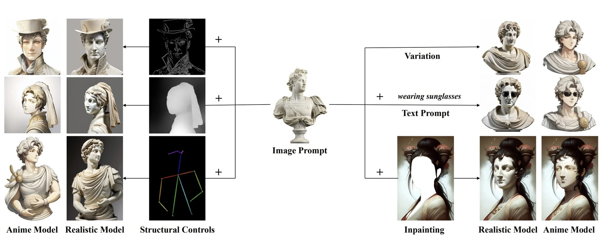
Key Architectural Components and Detailed Integration
- Image Encoder and Global Embedding: The reference image is processed using a frozen vision encoder—typically OpenCLIP-ViT-H/14—which outputs a single global embedding vector \( e_{\mbox{img}} \in \mathbb {R}^D \). This vector captures high-level visual semantics such as identity, global composition, and stylistic intent. Note that \( D \) (e.g., 1024 for ViT-H/14) typically differs from the internal dimension \( d \) of the U-Net’s cross-attention layers (e.g., 768 in Stable Diffusion 1.5). Thus, a transformation is needed to bridge this dimensional gap.
-
Projection to Visual Tokens (\( \phi \)): Since the U-Net expects a sequence of \( N \) key/value tokens, each of dimension \( d \), IP-Adapter introduces a lightweight, trainable projection network: \[ \phi \colon \mathbb {R}^D \rightarrow \mathbb {R}^{N \times d} \] which maps the global image embedding \( e_{\mbox{img}} \) into a sequence of \( N \) visual tokens: \[ [c_1, \ldots , c_N] = \phi (e_{\mbox{img}}), \quad \mbox{with } c_i \in \mathbb {R}^d. \]
- Why Use \( N > 1 \): Multiple visual tokens enable the model to attend separately to different latent attributes of the reference image—such as pose, color palette, facial features, or overall scene layout. This mirrors how textual prompts are split into subword tokens, each contributing distinct semantic signals. A typical choice is \( N = 4 \), balancing diversity of representation with computational efficiency.
-
Structure of \( \phi \): The projection network consists of a single linear layer followed by Layer Normalization: \[ \phi (e_{\mbox{img}}) = \mbox{LayerNorm}(W_\phi e_{\mbox{img}}), \quad \mbox{with } W_\phi \in \mathbb {R}^{(N \cdot d) \times D} \] The result is reshaped into a matrix in \( \mathbb {R}^{N \times d} \). The LayerNorm is applied across token dimensions and serves two key purposes:
- 1.
- Statistical stability: It normalizes the projected tokens, reducing internal covariate shift and promoting smoother gradient flow during training.
- 2.
- Architectural compatibility: It aligns the statistics of the visual tokens with those of the text encoder, which are also typically normalized. This facilitates better integration into the pretrained U-Net’s attention layers, which expect normalized key/value inputs.
-
Parallel Cross-Attention Layers: Let \( Z \in \mathbb {R}^{L \times d} \) denote the input query features from an intermediate U-Net block, and let \( c_t \in \mathbb {R}^{T \times d} \) be the tokenized text embeddings from the frozen CLIP text encoder. The original cross-attention mechanism in the pretrained U-Net computes:
\[ Z' = \mathrm {Attention}(Q, K, V) = \mathrm {Softmax}\left ( \frac {QK^\top }{\sqrt {d}} \right ) V, \] where \[ Q = Z W_q, \quad K = c_t W_k, \quad V = c_t W_v, \] and \( W_q, W_k, W_v \in \mathbb {R}^{d \times d} \) are the frozen projection matrices.
To introduce visual conditioning, IP-Adapter appends a decoupled image-specific attention stream using the same queries \( Q \), but separate keys and values derived from the projected image token sequence \( c_i \in \mathbb {R}^{N \times d} \): \[ Z'' = \mathrm {Attention}(Q, K', V') = \mathrm {Softmax}\left ( \frac {Q K'^\top }{\sqrt {d}} \right ) V', \] where \[ K' = c_i W'_k, \quad V' = c_i W'_v, \] and \( W'_k, W'_v \in \mathbb {R}^{d \times d} \) are new trainable projection matrices. These are typically initialized from \( W_k \) and \( W_v \) to accelerate training convergence.
- Fusion Strategy: The outputs of the text-guided and image-guided attention modules are combined additively: \[ Z_{\mbox{new}} = Z' + \lambda \cdot Z'', \] where \( \lambda \in \mathbb {R} \) is a tunable scalar controlling the influence of the image prompt. At inference time, adjusting \( \lambda \) allows for fine-grained control over the visual guidance: \( \lambda = 1 \) yields full conditioning on the image prompt, while \( \lambda = 0 \) recovers the original text-only generation behavior.
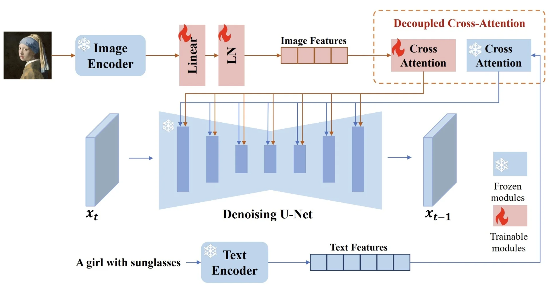
Versatility and Generalization without Fine-Tuning A key strength of the IP-Adapter architecture lies in its remarkable generalization and composability. Once trained, the adapter can be reused across a wide variety of downstream tasks without requiring any task-specific fine-tuning. It remains compatible with community models built upon the same base U-Net backbone (e.g., Stable Diffusion v1.5) and can be combined seamlessly with structured conditioning mechanisms such as ControlNet [794].
This flexibility is enabled by IP-Adapter’s non-invasive, modular design. Its decoupled attention layers are appended orthogonally to the pretrained U-Net, and its lightweight projection network transforms the reference image into a short sequence of visual tokens. These tokens serve as semantic key–value embeddings that are injected into the added image-specific attention stream. Because the architecture avoids modifying the backbone U-Net or interfering with the frozen text encoder, it remains interoperable with other conditioning systems that operate on different modalities.
For example, when paired with ControlNet, the model can synthesize images that respect both high-level semantic intent (from the image prompt) and low-level spatial structure (from edge maps, depth, or pose). The semantic tokens from IP-Adapter modulate subject identity, style, and appearance, while the structured control map—processed through a parallel ControlNet—anchors the generation to a target layout. These influences act concurrently: one guiding what should appear, the other guiding how and where it should appear.
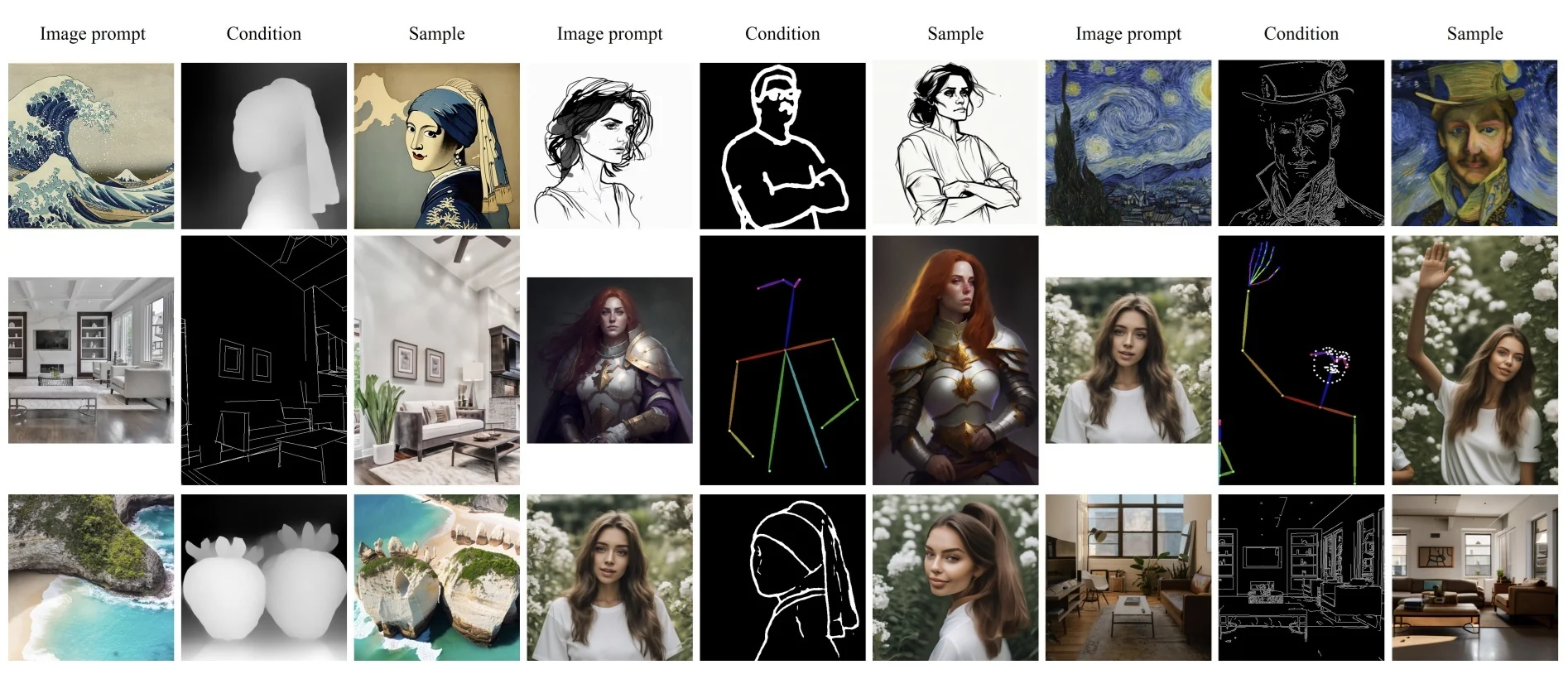
As illustrated in Figure 20.124, this compositional capability allows users to generate coherent, high-fidelity outputs where appearance and structure are jointly controlled. The adapter generalizes across visual styles, domains, and control inputs with no need to retrain for specific downstream tasks. This makes it a practical and powerful tool in real-world creative workflows, where flexibility, reuse, and modularity are critical.
Comparative Evaluation Across Structural Control Tasks To further validate its adaptability and effectiveness, IP-Adapter was comprehensively benchmarked against a wide range of alternative methods across multiple structural generation tasks. These competing approaches span three major categories:
- Trained-from-scratch models, such as Open unCLIP [524], Kandinsky-2.1 [548], and Versatile Diffusion [739], which are optimized end-to-end for joint image-text alignment.
- Fine-tuned models, including SD Image Variations [609] and SD unCLIP [610], which adapt pretrained diffusion models for image prompt inputs via extensive retraining.
- Adapter-based solutions, such as the Style Adapter of T2I-Adapter [456], Uni-ControlNet’s global controller [811], SeeCoder [738], and variants of ControlNet [794] (e.g., ControlNet-Reference and ControlNet-Shuffle), which inject image conditioning in a modular fashion.
Unlike methods that require task-specific retraining or rely on dedicated control structures for each condition type, IP-Adapter achieves competitive or superior results using a single, unified architecture. It supports a wide range of conditioning tasks—such as edge-to-image translation, sketch-to-style synthesis, and pose-guided generation—without retraining for each setup.
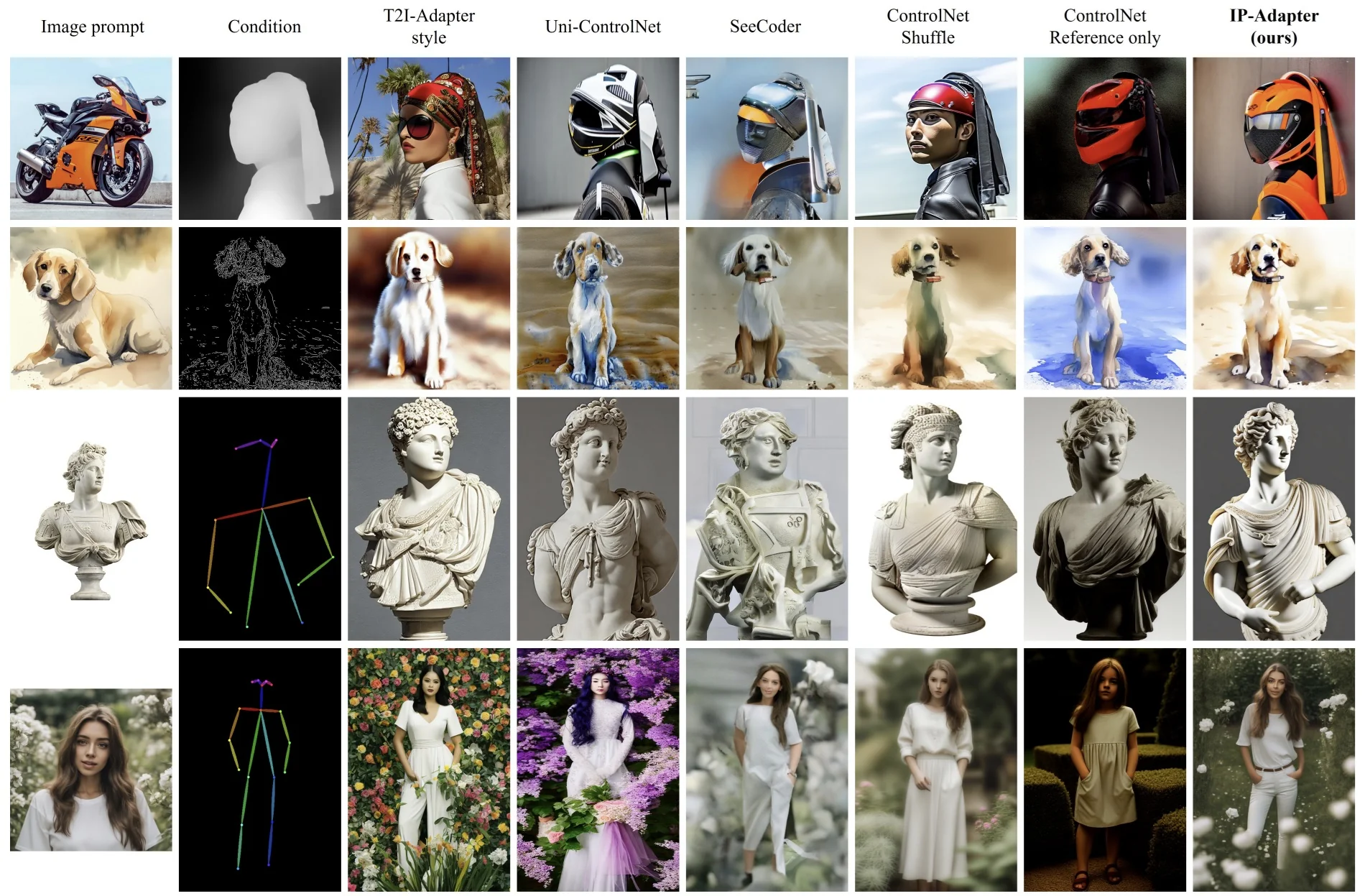
Image-to-Image Translation, Inpainting, and Multimodal Prompting IP-Adapter’s inherent strength lies in its remarkable versatility: it enables a single architecture with fixed parameters to adapt seamlessly across diverse image generation paradigms [755]. This includes high-quality image-to-image translation, image inpainting, and multimodal prompting, where both image and text jointly guide the generation process.
For image-to-image translation, diffusion pipelines often adopt strategies like SDEdit [434], which leverage stochastic differential equations to perform controlled image editing. Instead of generating an image from pure noise, SDEdit begins with a real image and adds a calibrated amount of noise to partially erase its content. The resulting noised image is then denoised under new conditions—such as a modified prompt or altered guidance signals—enabling flexible and constrained editing.
Within this framework, IP-Adapter contributes as a semantic controller. The image prompt is passed through a frozen CLIP encoder and a projection module to extract a dense embedding representing the identity, style, and global appearance of the subject. These embeddings are injected into the U-Net via dedicated cross-attention layers, enriching the denoising trajectory with semantic cues. Crucially, the structural integrity of the original input is preserved, since the spatial information is derived directly from the partially noised source image, not from external conditioning modules like ControlNet. This allows IP-Adapter to achieve high-fidelity transformations—preserving fine-grained appearance details.
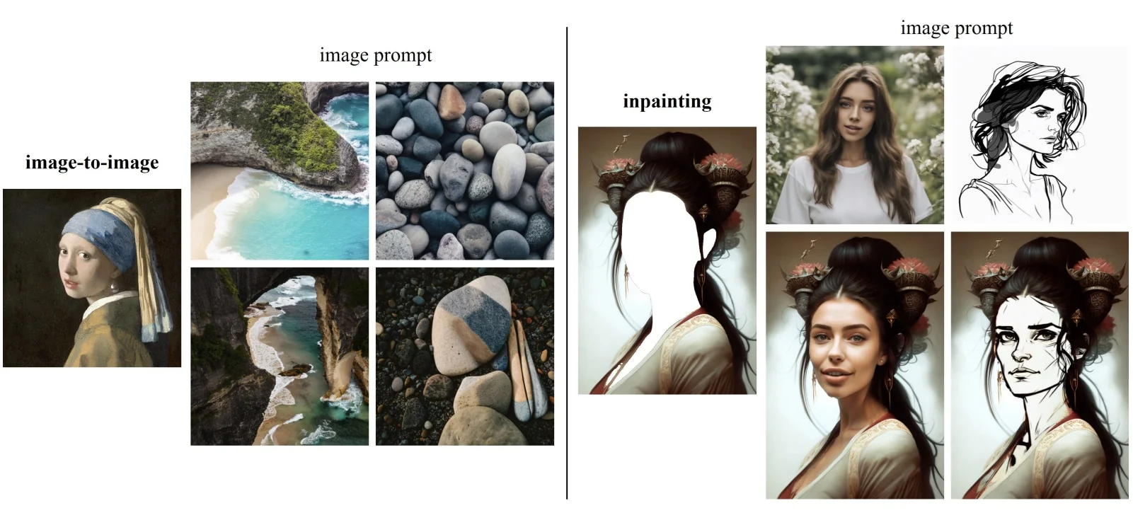
For inpainting, a related mechanism is used: a portion of the input image is masked and replaced with noise, and the diffusion model fills in the missing region during the denoising process. IP-Adapter enhances this process by injecting semantic guidance from the reference image prompt, ensuring that the inpainted content remains faithful to the original subject’s identity, lighting conditions, and stylistic attributes. This is particularly useful in creative tasks such as occlusion removal, selective editing, or visual reimagination, where both consistency and controllability are paramount.
The same IP-Adapter architecture also supports multimodal prompting, where both an image and a text prompt jointly influence generation. This enables fine-grained and compositional control: the image prompt preserves visual identity, style, and structural cues, while the text prompt modulates high-level semantics—such as adding new attributes, changing scene context, or modifying object categories. Unlike fully fine-tuned image prompt models, which often lose their text-to-image capability, IP-Adapter retains both modalities and allows users to balance their influence via the inference-time weight \( \lambda \).
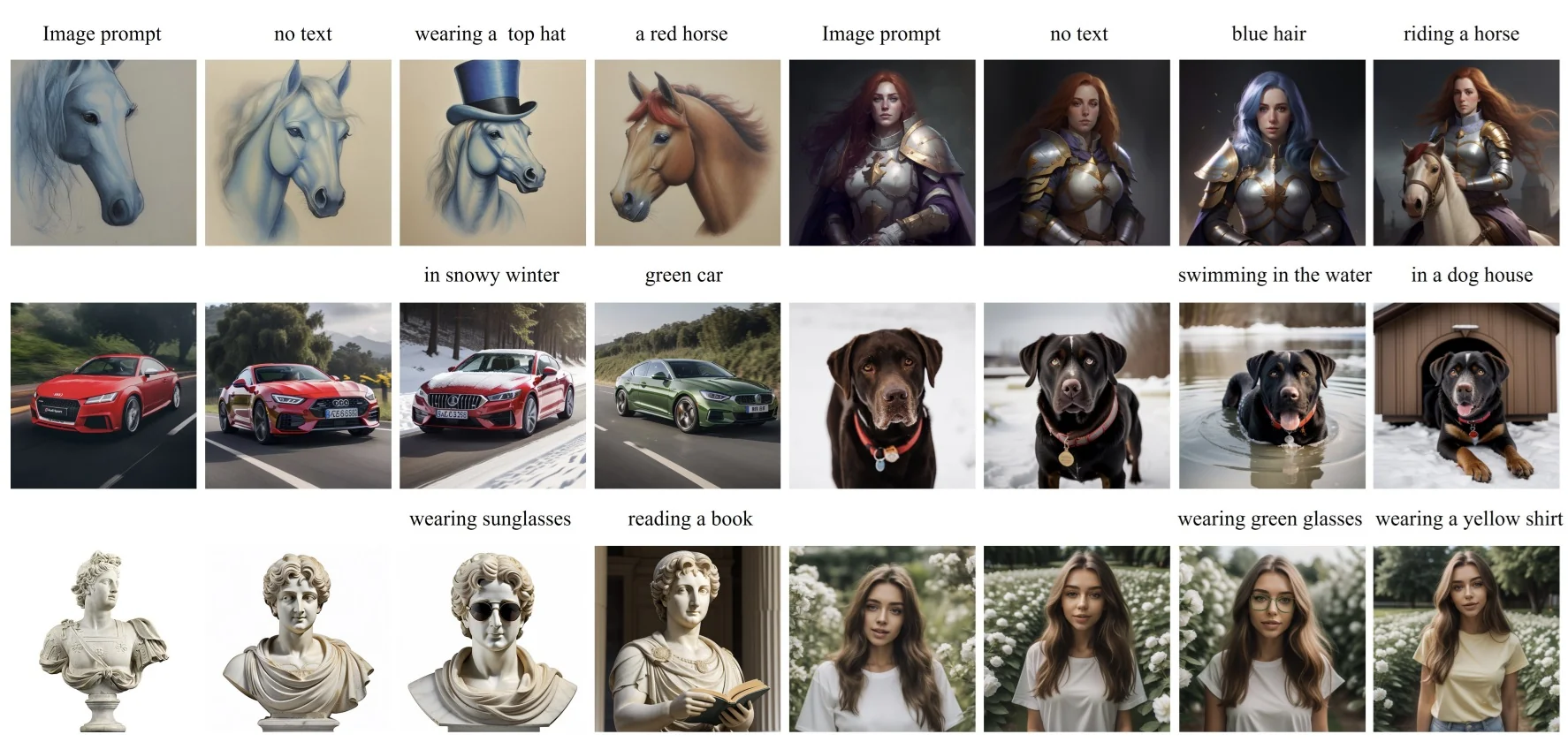
The synergy between image and text inputs makes IP-Adapter highly suitable for personalized and controllable generation scenarios. As we will now see, IP-Adapter also outperforms several multimodal baselines in this setting.
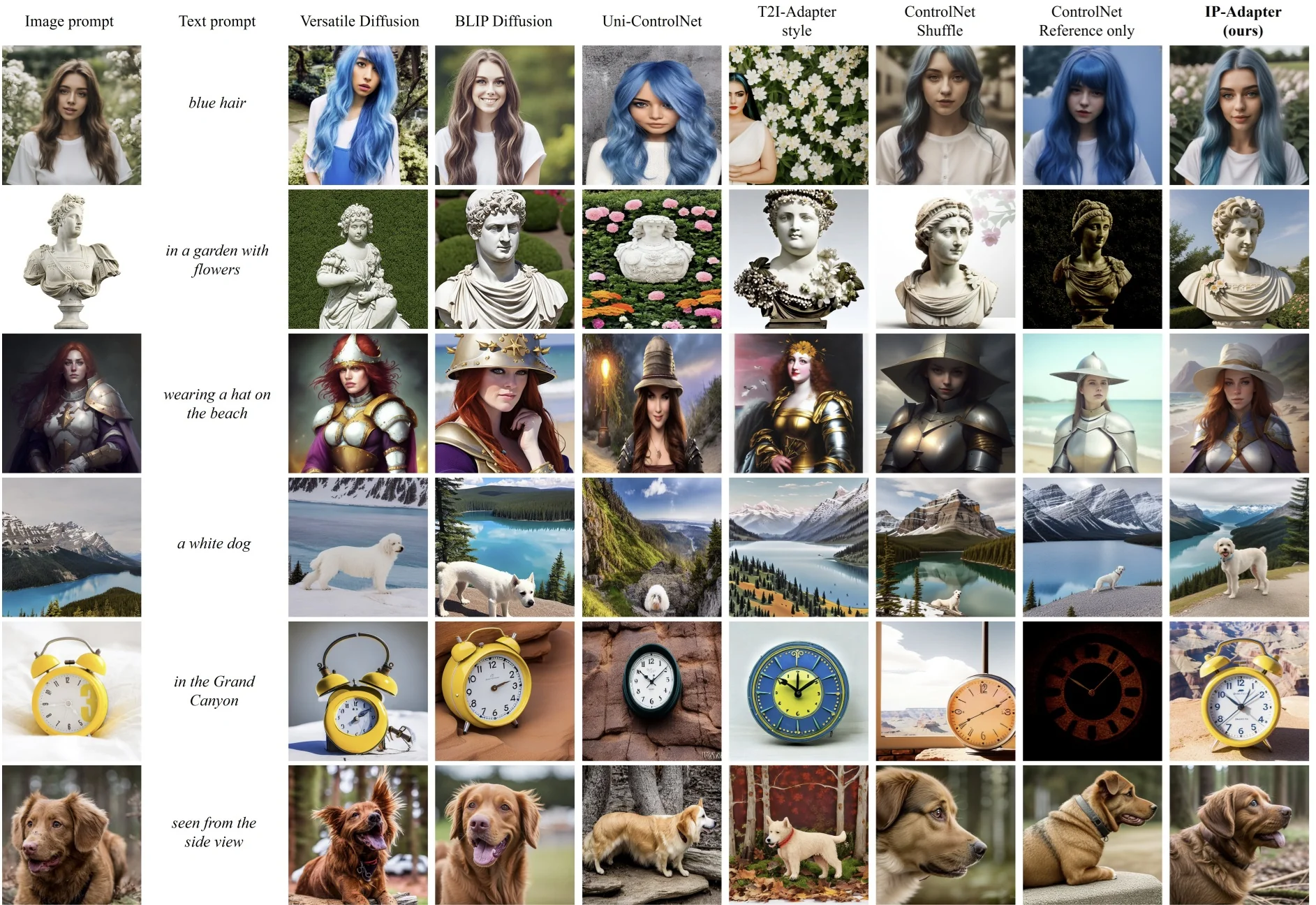
Figure 20.128 provides qualitative comparisons with competing methods for multimodal image generation. The results show that IP-Adapter produces images that better preserve identity, maintain high visual quality, and more faithfully follow both text and image prompts compared to BLIP-Diffusion, T2I-Adapter, and Uni-ControlNet.
In the next part, we explore ablation studies that demonstrate how IP-Adapter’s core architectural choices—including decoupled attention and feature granularity—affect the quality and controllability of generations.
Ablation: Validating Architectural Design To assess the effectiveness of its key architectural decisions, the IP-Adapter paper includes a set of controlled ablation experiments. These studies highlight the contribution of the decoupled cross-attention mechanism and investigate the trade-offs between different feature representations used in the adapter.
Baseline Comparison: Simple Adapter without Decoupling
A natural baseline is to compare IP-Adapter against a simpler variant that
injects image features using the existing text cross-attention layers—without the
decoupled attention pathway. While this approach simplifies integration, it suffers
from feature entanglement and capacity conflict between modalities.
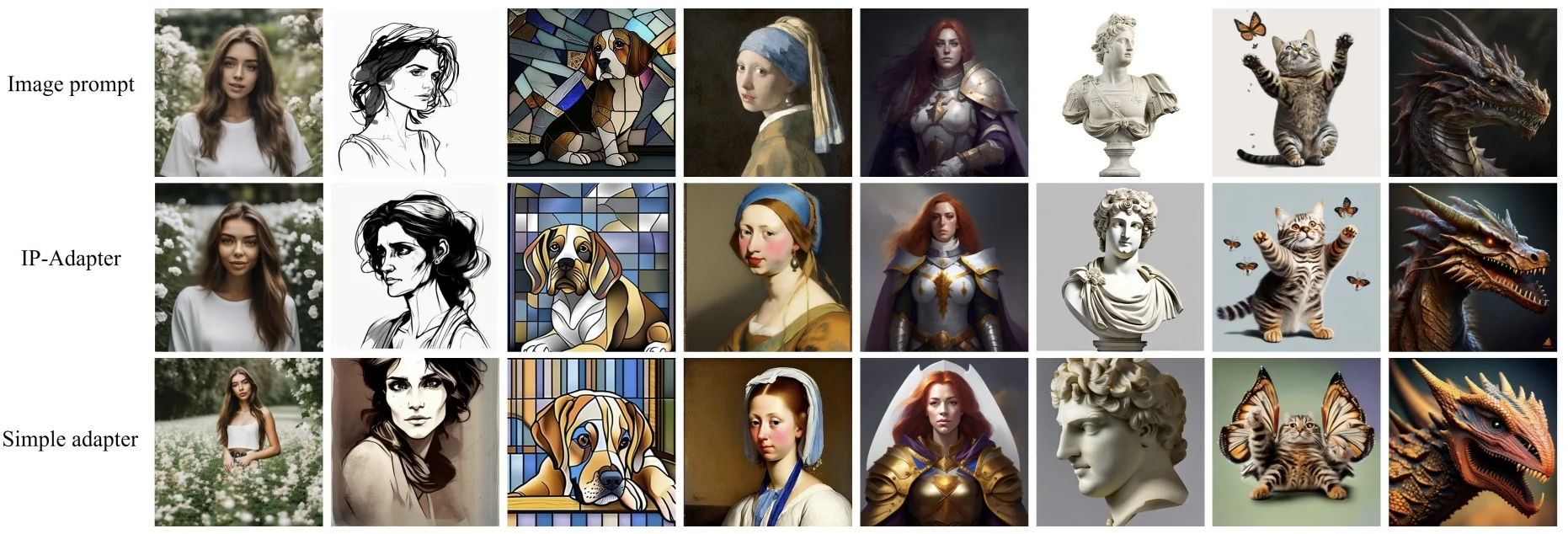
As shown in Figure 20.129, the simple adapter baseline often struggles to preserve subject identity and generates content that deviates from the image prompt. In contrast, IP-Adapter achieves high alignment with the source image, demonstrating the necessity of modality separation for accurate multimodal fusion.
Granularity of Image Representations: Global vs. Fine-Grained Tokens
A key design decision in IP-Adapter is the choice of granularity for representing the image prompt. By default, the adapter extracts a single global CLIP embedding from the reference image and projects it into a small sequence of visual tokens (typically \( N = 4 \)). These tokens are then injected into the U-Net’s cross-attention layers to guide generation. This setup provides a lightweight and expressive way to convey high-level semantics—such as identity, style, and layout—while remaining efficient and generalizable.
To investigate whether more detailed spatial alignment could be achieved, the IP-Adapter authors explored an alternative design that uses fine-grained visual tokens. Instead of relying solely on the global embedding, this variant extracts grid features from the penultimate layer of the frozen CLIP vision encoder. These grid features retain localized spatial information and are processed by a lightweight transformer query network, which learns to distill them into a sequence of 16 learnable visual tokens. These finer-grained tokens are then used in the same cross-attention mechanism, replacing the global-token projection.
Experimental Setup and Trade-offs: This variant was trained on the same dataset and evaluated under identical generation settings to allow fair comparison with the global-token version. The results, shown in the following figure, highlight a clear trade-off. The fine-grained configuration improves consistency with the reference image, particularly in background structures and subtle textures. However, it also tends to constrain the generative process more tightly, leading to reduced diversity across output samples. In contrast, the default global-token design offers a strong balance between semantic fidelity and output variation, making it better suited for general-purpose use.
Importantly, this limitation in diversity with fine-grained tokens can often be mitigated by adding complementary conditioning—such as text prompts or ControlNet structural maps—which help guide the generative process while restoring flexibility. In practice, the global-token configuration remains the preferred choice for most applications due to its simplicity, efficiency, and broader compatibility with multimodal workflows.
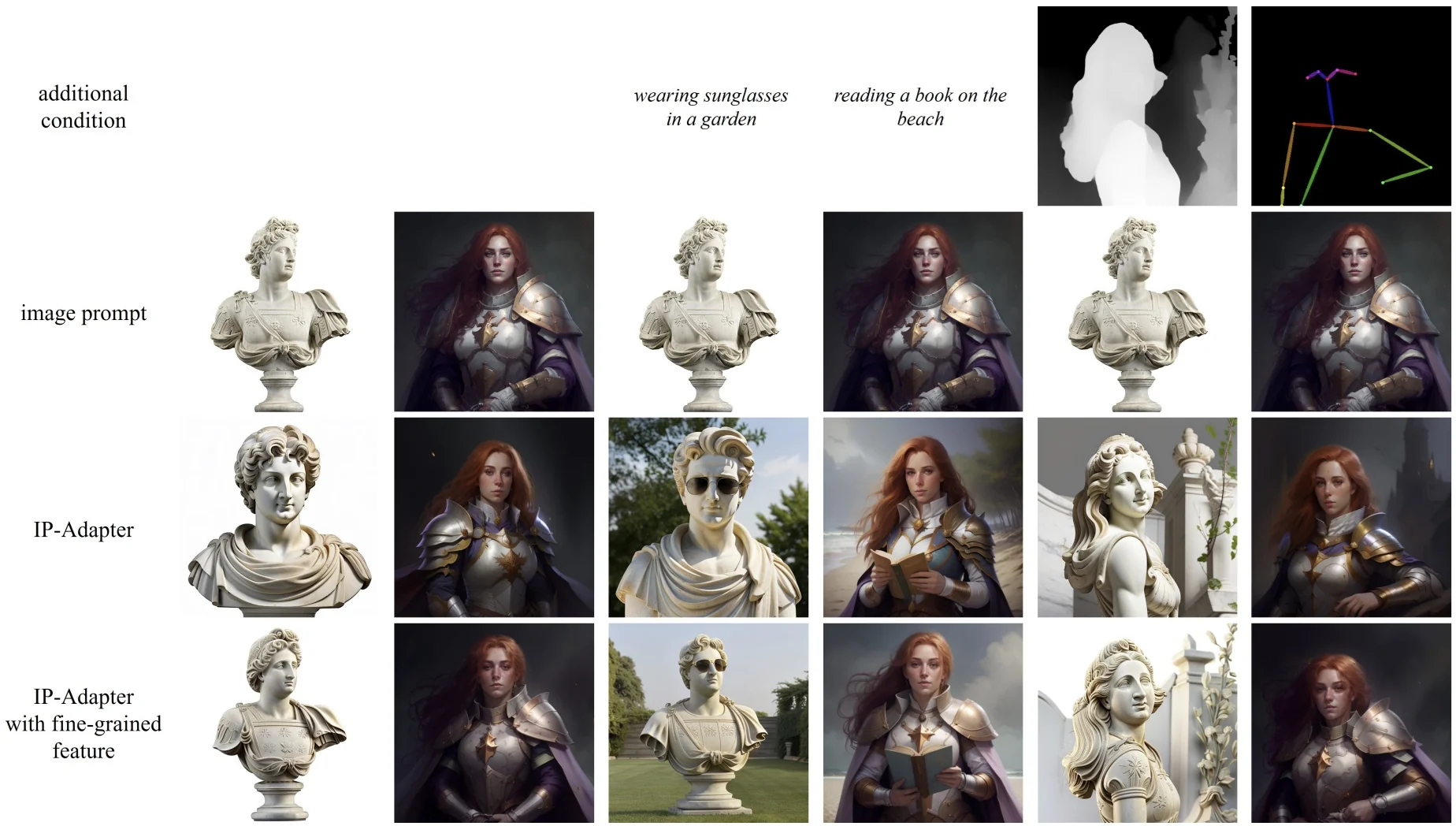
These ablation studies confirm that both the decoupled architecture and the choice of token granularity play critical roles in the model’s performance. The modularity of IP-Adapter allows these components to be tailored depending on the intended use—whether for faithful recreation, stylized adaptation, or diverse sampling.
Looking Forward A core motivation behind IP-Adapter was to disentangle heterogeneous modalities—specifically, to inject visual semantics directly via image embeddings rather than forcing them through the linguistic bottleneck of text encoders. This decoupling resolved key limitations in early diffusion pipelines, where all conditioning—even image-derived information—had to pass through shared cross-attention layers, often degrading fidelity and limiting semantic expressiveness. By introducing dedicated visual pathways that operate alongside the frozen U-Net, IP-Adapter preserved both the semantic richness of image prompts and the integrity of pre-trained text-to-image capabilities [755].
While this modular design proved highly effective for visual prompting, it was never meant to support fully compositional control across multiple modalities. As use cases grow more complex—demanding joint integration of reference appearance, structural layout, and descriptive language—the limitations of modularity become increasingly evident. Combining multiple modules (e.g., IP-Adapter for visual identity, ControlNet for edges or pose, and a separate module for text) introduces architectural overhead, modality-specific constraints, and potential conflicts between independently routed guidance signals. Each modality is still handled in isolation, with no mechanism for learning their mutual interactions or resolving contradictions.
This has sparked a broader shift toward unified conditioning frameworks—architectures designed to ingest and fuse all input modalities within a single attention-driven latent space. Rather than bolting on more specialized adapters, these frameworks are trained end-to-end on mixed-modality sequences, allowing them to learn how different types of guidance interact, reinforce, or compete.
A compelling example of this conceptual leap is Transfusion [828], which we examine next. Whereas IP-Adapter introduces decoupled cross-attention to avoid modality entanglement, Transfusion instead embraces entanglement through a shared modeling framework. It trains a single transformer to jointly model discrete text tokens and continuous image patches as part of a unified sequence, using shared self-attention and feedforward layers across modalities. This enables the model to perform both language modeling and diffusion denoising within the same architecture—dissolving the boundaries that modular adapters merely isolate.
By learning to align and synthesize multimodal signals within a single generative process, Transfusion opens the door to richer, more coherent compositionality and seamless modality interaction—without the overhead of managing separate modules. It represents the natural evolution of multimodal generation: not just retrofitting existing systems with external guidance, but rethinking the generative architecture itself from the ground up.
Enrichment 20.11.10: Transfusion: Unified Multimodal Generation
Motivation and Overview Generative models have reached state-of-the-art performance in individual modalities: large language models (LLMs) like GPT excel at producing coherent and contextually rich text, while diffusion-based models such as Stable Diffusion generate highly realistic images. However, building a unified generative system capable of seamlessly reasoning across both text and image modalities remains a significant challenge.
Existing approaches to multimodal generation typically fall into one of two categories:
- Discrete Tokenization of Images: Approaches like DALL·E [525] or Chameleon [410] quantize images into discrete visual tokens (e.g., via VQ-VAEs), allowing them to be modeled autoregressively like text. While effective, this discretization introduces information loss and reduces the fidelity of visual synthesis.
- Modular Pipelines: Methods such as IP-Adapter [755] or ControlNet [794] augment existing text-to-image diffusion models with auxiliary components that inject conditioning signals. While flexible, these grafted architectures often lack global coherence, require per-modality customization, and struggle with joint, end-to-end reasoning.
Such designs are often brittle, especially when dealing with interleaved inputs (e.g., text-image-text) or outputs requiring fine cross-modal consistency.
Transfusion [828] overcomes these limitations with a clean and elegant solution: a single, modality-agnostic transformer trained end-to-end to model mixed sequences of text and image content. Rather than building separate encoders or injecting one modality into another, Transfusion unifies both within a shared token stream and a shared network backbone. It achieves this via two key design principles:
- Shared Transformer Backbone: A single transformer with shared weights processes both text tokens and continuous image patch embeddings. This facilitates uniform attention over all elements in the sequence and supports tight cross-modal interactions.
- Dual Training Objectives: The model is jointly trained with a language modeling loss (for text) and a denoising diffusion loss (for image patches). The training procedure teaches the model to predict the next text token and remove noise from corrupted image tokens—both using the same architecture.
This unified formulation enables Transfusion to support a wide range of input-output formats with a single model:
- Text \(\rightarrow \) Image: Text-to-image generation.
- Image \(\rightarrow \) Text: Image captioning and visual understanding.
-
Mixed \(\rightarrow \) Mixed: One of the most compelling strengths of Transfusion is its ability to process and generate rich interleaved sequences of text and images. These tasks involve both multimodal inputs and multimodal outputs—handled in a unified transformer pipeline. Such capabilities are essential for:
-
Visual storytelling: Given a sequence of text snippets—such as narrative sentences, scene descriptions, or story fragments—the model generates a coherent visual story by producing aligned image segments after each text block. Conversely, it can also generate interleaved text commentary or narrative lines from a sequence of input images.
For example:
"A boy opens a mysterious book." <BOI> image_1 <EOI>
"A portal begins to glow on the wall." <BOI> image_2 <EOI>
"He steps through, entering a dreamlike jungle." <BOI> image_3 <EOI>Each element is contextually grounded in prior ones, and the sequence evolves in both text and image domains, preserving temporal and semantic coherence.
- Multimodal dialog: The model supports dynamic interactions where inputs and outputs alternate between text and images. For instance, a user may submit an image followed by a question, and the model replies with a mix of visual and textual responses—such as diagrams, sketches, or annotated outputs. This enables applications in tutoring, grounded question answering, and multimodal assistants.
-
Text-guided image editing and inpainting: Given an input image and a text instruction, the model directly generates a modified image that reflects the desired edit, without requiring separate control modules or manually designed conditioning maps:
"Replace the red car with a bicycle." <BOI> edited_image <EOI>
These scenarios are challenging for traditional diffusion models, and some scenarios are challenging to even adapter-augmented architectures (e.g., ControlNet [794], IP-Adapter [755]). Such modular systems often lack the flexibility to process arbitrary multimodal sequences or to maintain cross-modal consistency across multiple alternating steps of generation.
In contrast, Transfusion achieves this by treating text tokens and continuous image tokens as part of the same autoregressive token sequence. The model does not differentiate between modalities at the architectural level—only special delimiter tokens (e.g., <BOI> (Beginning of Image), <EOI> (End of Image)) indicate modality boundaries. All tokens are processed uniformly using shared transformer layers, and multimodal coherence is learned end-to-end via joint training with language modeling and diffusion objectives.
This design enables the model to naturally reason over long multimodal contexts, propagate dependencies across modality transitions, and generate semantically aligned outputs that respect both linguistic structure and visual consistency.
-
Architecture and Training Pipeline of Transfusion To understand the unified nature of Transfusion, we now examine its complete generative pipeline—starting from raw image and text inputs, proceeding through tokenization and transformer processing, and culminating in joint modality-specific losses. This breakdown serves as the foundation for later sections covering generation and editing capabilities.
Part 1: Image Tokenization Pipeline To enable seamless multimodal generation, Transfusion converts images into continuous, transformer-compatible tokens that can be interleaved with discrete text tokens. This process preserves the spatial structure and rich visual semantics of the input while allowing joint processing by a single transformer.
-
Spatial Encoding via Convolutional VAE: The input image \( x \in \mathbb {R}^{H \times W \times 3} \) is passed through a pretrained convolutional Variational Autoencoder (VAE) [304], which encodes it into a lower-resolution latent feature map. The encoder is composed of stacked convolutional layers that downsample the image by a factor of \( s \), producing two tensors: \[ \mu (x), \log \sigma ^2(x) \in \mathbb {R}^{H' \times W' \times d}, \quad \mbox{with} \quad H' = H/s, \, W' = W/s \] Each spatial location \( (i,j) \) corresponds to a receptive field in the original image and defines a diagonal Gaussian distribution: \[ q(z_{i,j} \mid x) = \mathcal {N}(z_{i,j} \mid \mu _{i,j}, \sigma _{i,j}^2 \cdot I_d) \] During VAE training, latent samples are drawn using the reparameterization trick: \[ z_{i,j} = \mu _{i,j} + \sigma _{i,j} \cdot \epsilon _{i,j}, \quad \epsilon _{i,j} \sim \mathcal {N}(0, I_d) \] The decoder then reconstructs the original image \( \hat {x} \approx x \). The loss combines a reconstruction objective with a KL divergence regularizer to promote a smooth latent space: \[ \mathcal {L}_{\mbox{VAE}} = \mathbb {E}_{q(z \mid x)} \left [ \| \hat {x} - x \|^2 \right ] + \beta \cdot \mathrm {KL}(q(z \mid x) \,\|\, p(z)) \]
During downstream use (e.g., tokenization in Transfusion), the VAE encoder is kept frozen and the sampling step is disabled. Instead, the deterministic mean \( z := \mu (x) \in \mathbb {R}^{H' \times W' \times d} \) is used as the spatially-structured latent representation. Each vector \( z_{i,j} \in \mathbb {R}^d \) serves as a dense, localized encoding of a specific region in the input image.
-
Patching Strategy for Tokenization: The latent tensor \( z \) is then transformed into a 1D sequence of patch-level embeddings using one of two methods:
- Linear Projection: The latent map is divided into non-overlapping \( k \times k \) spatial blocks, each containing \( k^2 \) adjacent vectors \( z_{i,j} \in \mathbb {R}^d \). Each block is flattened into a vector of shape \( k^2 \cdot d \), then passed through a linear layer that compresses it back to dimension \( d \). This method provides a direct, local embedding of visual content and is easy to implement, but it lacks contextual integration beyond each patch.
- U-Net-style Downsampling (Preferred): Alternatively, Transfusion applies a shallow convolutional encoder (often derived from the U-Net stem) to the full latent tensor \( z \). This module downsamples the spatial dimensions further (e.g., \( H' \to \tilde {H} \)), enabling each resulting token to summarize information over a broader receptive field. These richer embeddings are particularly beneficial for complex generation tasks that require high-level reasoning or long-range visual consistency.
- Token Sequence Construction: The resulting patch embeddings \( \{ z_1, \ldots , z_N \} \subset \mathbb {R}^d \) form a continuous image token sequence. These are either appended to or interleaved with discrete text tokens to form a unified input stream for the transformer. Special delimiter tokens (e.g., <BOI>, <EOI>) are inserted to mark modality boundaries, but the transformer processes all tokens jointly, enabling fluent multimodal generation and reasoning.
Part 2: Text Tokenization Pipeline The text prompt \(\mathcal {T}\) is first converted into a sequence of discrete tokens using a standard tokenizer, then embedded into the same feature space as the image tokens:
-
A Byte-Pair Encoding (BPE) tokenizer transforms the input string into a token sequence:
\[ \mathcal {T} \mapsto \{ w_1, w_2, \ldots , w_M \}, \quad w_i \in \mathcal {V}_{\mbox{text}} \]
-
Each token \(w_i\) is mapped to a continuous vector \(e_i \in \mathbb {R}^d\) using a learned embedding matrix \(E_{\mbox{text}} \in \mathbb {R}^{|\mathcal {V}_{\mbox{text}}| \times d}\):
\[ e_i = E_{\mbox{text}}[w_i] \]
-
This produces the text embedding sequence:
\[ x_{\mbox{text}} = [e_1, e_2, \ldots , e_M] \in \mathbb {R}^{M \times d} \]
Part 3: Multimodal Sequence Construction After obtaining both the image token sequence \(x_{\mbox{img}} = [z_1, z_2, \ldots , z_N] \in \mathbb {R}^{N \times d}\) from Part 1 and the text token embeddings \(x_{\mbox{text}} \in \mathbb {R}^{M \times d}\) from Part 2, Transfusion constructs a unified input sequence for the transformer.
-
Two special learnable embeddings are added to delimit the image region:
\[ e_{\texttt{<BOI>}}, \quad e_{\texttt{<EOI>}} \in \mathbb {R}^d \]
-
The final multimodal input to the transformer is the concatenation:
\[ x_{\mbox{input}} = [e_1, \ldots , e_M, e_{\texttt{<BOI>}}, z_1, \ldots , z_N, e_{\texttt{<EOI>}}] \in \mathbb {R}^{(M+N+2) \times d} \]
- Optional position encodings or segment embeddings may be added to indicate token roles and preserve modality structure.
Part 4: Transformer Processing with Hybrid Attention A single transformer autoregressively processes the multimodal sequence \(x_{\mbox{input}}\). To balance generation constraints with spatial reasoning, Transfusion adopts a hybrid attention mask:
- Causal attention is applied globally, ensuring that each token can only attend to previous tokens in the sequence.
- Bidirectional attention is enabled locally within the image region delimited by <BOI> and <EOI>, allowing all image tokens to attend to one another.
This hybrid masking strategy preserves autoregressive generation for the full sequence while enabling richer spatial reasoning among image tokens—improving sample fidelity and multimodal alignment.
Part 5: Training Objectives and Loss Functions Transfusion jointly optimizes a unified transformer model over both text and image inputs. The training procedure integrates two complementary objectives—autoregressive language modeling and latent-space denoising—applied respectively to text tokens and VAE image patches. These objectives are optimized simultaneously using shared model parameters, with losses computed over the appropriate modality regions in the input sequence.
-
Text Modeling Loss \(\mathcal {L}_{\mbox{text}}\): For positions in the sequence corresponding to text tokens \(\{ w_1, \ldots , w_M \}\), the model is trained to predict each next token \(w_{i+1}\) based on the preceding context \(w_{\leq i}\), using standard autoregressive language modeling.
\[ \mathcal {L}_{\mbox{text}} = - \sum _{i=1}^{M} \log p(w_{i+1} \mid w_{\leq i}) \]
The prediction is compared against the ground truth token from the training data, and the loss is computed as cross-entropy between the predicted distribution and the true next-token index. This formulation ensures that the model learns to generate fluent, contextually appropriate text conditioned on both prior tokens and (when available) image content.
-
Image Denoising Loss \(\mathcal {L}_{\mbox{diff}}\): For image regions—i.e., the continuous sequence of tokens \(z_0 \in \mathbb {R}^{N \times d}\) obtained by encoding and optionally downsampling the image with a pretrained VAE—the model is trained using a DDPM-style denoising objective.
During training, a timestep \(t \sim \{1, \ldots , T\}\) is sampled, and Gaussian noise is added to each image token \(z_0^{(j)} \in \mathbb {R}^d\) using the forward diffusion process:
\[ z_t^{(j)} = \sqrt {\bar {\alpha }_t} \, z_0^{(j)} + \sqrt {1 - \bar {\alpha }_t} \, \epsilon ^{(j)}, \quad \epsilon ^{(j)} \sim \mathcal {N}(0, I) \]
Here, \(\bar {\alpha }_t\) is a cumulative noise schedule, and \(\epsilon ^{(j)}\) is the sampled noise used to corrupt patch \(j\). The model is trained to predict \(\epsilon ^{(j)}\) from \(z_t^{(j)}\) and the timestep \(t\), minimizing the mean squared error over all patches:
\[ \mathcal {L}_{\mbox{diff}} = \mathbb {E}_{t, z_0, \epsilon } \left [ \frac {1}{N} \sum _{j=1}^{N} \left \| \epsilon _\theta (z_t^{(j)}, t) - \epsilon ^{(j)} \right \|_2^2 \right ] \]
This loss operates entirely in latent space; no decoding to pixels is performed during training. The ground truth for each position is the actual noise added in the forward process. The use of VAE latents enables spatial preservation and compact representation, making the diffusion process more efficient than pixel-level alternatives.
-
Total Training Loss \(\mathcal {L}_{\mbox{total}}\): The overall training objective combines both modality-specific terms into a weighted sum:
\[ \mathcal {L}_{\mbox{total}} = \lambda _{\mbox{text}} \cdot \mathcal {L}_{\mbox{text}} + \lambda _{\mbox{diff}} \cdot \mathcal {L}_{\mbox{diff}} \]
where \(\lambda _{\mbox{text}}, \lambda _{\mbox{diff}} \in \mathbb {R}_{\geq 0}\) are scalar coefficients that control the relative contribution of text modeling and image denoising to the final loss. In practice, the original Transfusion paper reports using \(\lambda _{\mbox{diff}} = 5\), giving higher weight to the image denoising component due to its higher dynamic range and training complexity.
Part 6: Key Advantages of the Training Design
- Full parameter sharing: No modality-specific blocks; language and vision share all layers.
- End-to-end joint training: All gradients flow through shared transformer, improving alignment.
- No discrete quantization: Image patches remain continuous, avoiding codebook collapse or token artifacts.
- Multimodal generation in a single pass: A single forward pass can generate image and text jointly.
Empirical Results and Qualitative Examples
Showcase: High-Quality Multi-Modal Generation One of the most compelling outcomes of the Transfusion model is its ability to generate high-fidelity, semantically grounded images from a wide range of compositional text prompts. Trained with 7B parameters on a dataset of 2 trillion multimodal tokens—including both text and images—the model produces coherent and visually expressive outputs that exhibit stylistic nuance, spatial awareness, and fine-grained linguistic alignment.
These qualitative results demonstrate not only stylistic diversity but also compositional understanding—a hallmark of strong multimodal reasoning. Unlike U-NET based diffusion architectures that rely on external encoders or modality-specific adapters, Transfusion achieves this performance using a single, unified transformer trained from scratch, without separate alignment stages or handcrafted prompt tuning.
Zero-Shot Image Editing via Fine-Tuning Beyond text-to-image synthesis, Transfusion also generalizes to the task of image editing through lightweight fine-tuning. A version of the 7B model was adapted on a dataset of only 8,000 image–text pairs, each consisting of an input image and a natural-language instruction describing a desired change (e.g., “Remove the cupcake on the plate” or “Change the tomato on the right to a green olive”).
This result is notable: without requiring any architectural changes—such as inpainting masks or diffusion-specific guidance—the model learns to apply textual edit instructions directly. Training is end-to-end, and the only modification is through supervised adaptation on the editing dataset. This demonstrates the expressive capacity of the underlying sequence model and suggests extensibility to broader tasks such as viewpoint manipulation, object insertion, or multimodal storytelling.
Ablation Studies and Experimental Insights To evaluate the core design choices of Transfusion [818], the authors conduct extensive ablations over attention masking, patch size, encoder/decoder type, noise scheduling and model scale. Both vision and language benchmarks are reported with the metrics below.
Interpreting Evaluation Metrics
- PPL (Perplexity) \(\downarrow \): Measures uncertainty in language modeling. Lower values correspond to better next-token prediction performance.
- Accuracy (Acc) \(\uparrow \): Multiple-choice question answering accuracy, especially on LLaMA-style QA tasks.
- CIDEr \(\uparrow \): A captioning metric measuring consensus with human-written references, widely used in MS-COCO.
- FID (Fréchet Inception Distance) \(\downarrow \): Evaluates the visual realism of generated images. Lower is better. See Section 20.5.2.0 for a detailed explanation.
- CLIP Score \(\uparrow \): Measures semantic alignment between generated image and caption using pretrained CLIP embeddings [512].
Attention Masking: Causal vs. Bidirectional Bidirectional self-attention applied within each image notably improves FID for linear encoders (\(61.3\!\to \!20.3\)); U-Nets also benefit, though to a lesser extent.
| Encoder/Dec. | Attention | C4 PPL | Wiki PPL | Acc | CIDEr | FID | CLIP |
| Linear | Causal | 10.4 | 6.0 | 51.4 | 12.7 | 61.3 | 23.0 |
| Linear | Bidirectional | 10.4 | 6.0 | 51.7 | 16.0 | 20.3 | 24.0 |
| U-Net | Causal | 10.3 | 5.9 | 52.0 | 23.3 | 16.8 | 25.3 |
| U-Net | Bidirectional | 10.3 | 5.9 | 51.9 | 25.4 | 16.7 | 25.4 |
Patch Size Variations Larger patches reduce token length and compute, but can hurt performance. U-Nets are more robust than linear encoders.
| Encoder/Dec. | Patch | C4 PPL | Wiki PPL | Acc | CIDEr | FID | CLIP |
| Linear | \(1\times 1\) (1024) | 10.3 | 5.9 | 52.2 | 12.0 | 21.0 | 24.0 |
| Linear | \(2\times 2\) (256) | 10.4 | 6.0 | 51.7 | 16.0 | 20.3 | 24.0 |
| Linear | \(4\times 4\) (64) | 10.9 | 6.3 | 49.8 | 14.3 | 25.6 | 22.6 |
| Linear | \(8\times 8\) (16) | 11.7 | 6.9 | 47.7 | 11.3 | 43.5 | 18.9 |
| U-Net | \(2\times 2\) (256) | 10.3 | 5.9 | 51.9 | 25.4 | 16.7 | 25.4 |
| U-Net | \(4\times 4\) (64) | 10.7 | 6.2 | 50.7 | 29.9 | 16.0 | 25.7 |
| U-Net | \(8\times 8\) (16) | 11.4 | 6.6 | 49.2 | 29.5 | 16.1 | 25.2 |
Encoding Architecture: Linear vs. U-Net U-Nets outperform linear encoders across model sizes with only a modest parameter increase.
| Params | Encoder | C4 PPL | Wiki PPL | Acc | CIDEr | FID | CLIP |
| 0.76 B | Linear | 10.4 | 6.0 | 51.7 | 16.0 | 20.3 | 24.0 |
| U-Net | 10.3 | 5.9 | 51.9 | 25.4 | 16.7 | 25.4 | |
| 7.0 B | Linear | 7.7 | 4.3 | 61.5 | 27.2 | 18.6 | 25.9 |
| U-Net | 7.8 | 4.3 | 61.1 | 33.7 | 16.0 | 26.5 |
Noise Scheduling in Image-to-Text Training Capping diffusion noise to timesteps \(t\le 500\) improves CIDEr without degrading other metrics.
| Model | Cap \(t\le 500\) | C4 PPL | Wiki PPL | Acc | CIDEr | FID |
| 0.76 B | ✗ | 10.3 | 5.9 | 51.9 | 25.4 | 16.7 |
| 0.76 B | ✓ | 10.3 | 5.9 | 52.1 | 29.4 | 16.5 |
| 7.0 B | ✗ | 7.8 | 4.3 | 61.1 | 33.7 | 16.0 |
| 7.0 B | ✓ | 7.7 | 4.3 | 60.9 | 35.2 | 15.7 |
Comparison to Specialized Generative Models A single Transfusion model achieves strong performance on both image and text tasks compared with state-of-the-art specialised models.
| Model | Params | COCO FID\(\downarrow \) | GenEval\(\uparrow \) | Acc\(\uparrow \) | Modality | Notes |
| SDXL [496] | 3.4 B | 6.66 | 0.55 | – | Image | Frozen encoder |
| DeepFloyd IF [632] | 10.2 B | 6.66 | 0.61 | – | Image | Cascaded diffusion |
| SD3 [150] | 12.7 B | – | 0.68 | – | Image | Synthetic caps |
| Chameleon [829] | 7.0 B | 26.7 | 0.39 | 67.1 | Multi | Discrete fusion |
| Transfusion [818] | 7.3 B | 6.78 | 0.63 | 66.1 | Multi | Unified LM + diffusion |
Summary The ablation findings from [818] provide a clear picture of what makes Transfusion effective: bidirectional intra-image attention is key to spatial coherence; U-Net-based patch encoders contribute strong inductive biases that enhance both fidelity and alignment; and careful tuning of patch size and noise scheduling enables efficient training without compromising performance. The success of this architecture demonstrates that unifying text and image processing under a shared transformer with continuous embeddings is not only feasible but highly performant.
At the same time, the reliance on continuous image tokens and diffusion-based generation introduces additional training and sampling complexity. This raises a natural question: can we achieve the benefits of modality unification using simpler, fully discrete generation schemes? In the following section, we explore such a possibility through the lens of the VAR framework, which revisits token-level autoregressive modeling for unified image and text generation—offering a different perspective on multimodal generative design.
Enrichment 20.11.11: Visual Autoregressive Modeling (VAR)
Traditional autoregressive (AR) models, such as PixelCNN or transformer-based image generators, generate images sequentially by predicting each token (pixel, patch, or VQ code) in a predefined raster scan order—typically left to right and top to bottom. While conceptually straightforward, this strategy is fundamentally at odds with the two-dimensional nature of images and the hierarchical way humans perceive visual content.
Visual Autoregressive Modeling (VAR) [635] reconsiders how autoregression should operate in the image domain. Instead of modeling a 2D grid as a flattened 1D sequence, VAR predicts image content in a coarse-to-fine, multi-scale manner. At each scale, the model generates an entire token map in parallel, then conditions the next higher-resolution prediction on this coarser output. This process mirrors how humans often process visual inputs: first recognizing global structure, then refining local details.
This approach leads to multiple benefits:
- Improved efficiency: Tokens at a given resolution are predicted in parallel, which drastically reduces the number of autoregressive steps compared to raster-scan generation.
- Higher fidelity: Coarse-to-fine guidance encourages global coherence and fine-grained detail simultaneously.
- Scalable modeling: VAR exhibits smooth scaling behavior similar to language transformers, showing predictable gains as model and compute increase.
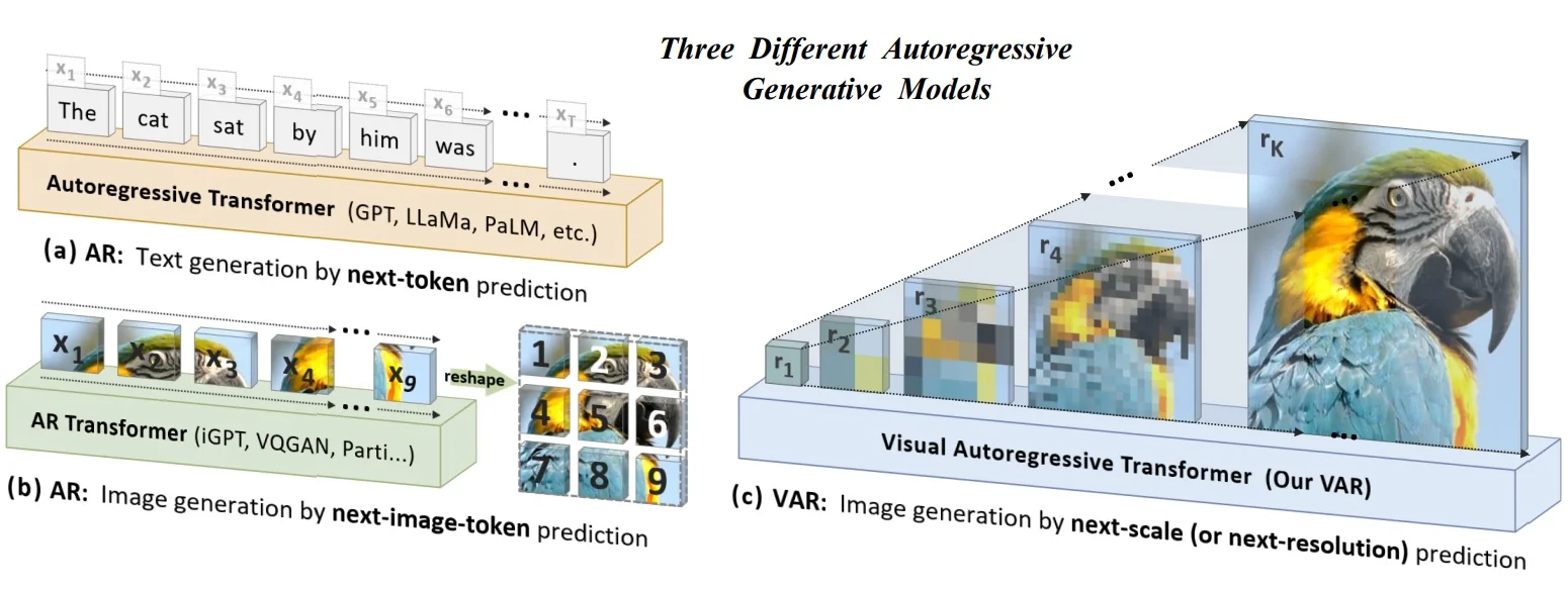
As we now explore, this paradigm shift from token-wise raster autoregression to scale-wise parallel prediction yields state-of-the-art results on ImageNet and opens the door to efficient, high-fidelity generation pipelines.
Multi-Scale Architecture for Coarse-to-Fine Generation: How VAR Works The core contribution of Visual Autoregressive Modeling (VAR) [635] is a paradigm shift in how autoregressive models approach image generation. Instead of predicting tokens in a strict raster-scan order—row-by-row, left to right—VAR proposes a coarse-to-fine, scale-based generation strategy that better reflects how humans compose images: beginning with global structure and refining toward detail. This section explains the architecture and training pipeline, focusing on the two foundational stages: hierarchical tokenization and scale-aware prediction.
Overview: A Two-Stage Pipeline for Image Generation The Visual AutoRegressive (VAR) model [635] tackles the problem of high-fidelity image generation using a modular, two-stage approach:
- Stage 1: Multi-Scale VQ-VAE for Hierarchical Tokenization Transforms a continuous image into a hierarchy of discrete tokens, each representing visual content at a different scale (from global layout to local texture). This compresses the image into symbolic representations that are more structured and compact than pixels or raw latent features.
- Stage 2: Scale-Aware Autoregressive Transformer Learns to model the joint distribution of token hierarchies and to autoregressively generate image tokens from coarse to fine, either unconditionally or conditioned on class/text input. This allows realistic, structured image synthesis without generating pixels directly.
These two stages are trained separately and serve complementary purposes:
- The VQ-VAE (Stage 1) learns how to discretize an image into multi-scale tokens \( R = (r_1, \dots , r_K) \) and how to reconstruct the image from them.
- The transformer (Stage 2) learns how to generate realistic sequences of these tokens, modeling \( p(r_1, \dots , r_K \mid s) \) where \( s \) is an optional conditioning signal.
This design addresses key challenges in autoregressive image modeling:
- It avoids operating over raw pixels, which are high-dimensional and redundant.
- It introduces scale-level causality, so image generation proceeds hierarchically (not raster-scan), yielding better spatial inductive structure.
- It separates representation learning (handled by the VQ-VAE) from generation (handled by the transformer), simplifying optimization and improving sample quality.
We now explain each stage in detail, beginning with the multi-scale encoding process of the VQ-VAE.
Stage 1: Multi-Scale VQ-VAE for Hierarchical Tokenization The first stage of the VAR pipeline [635] transforms a continuous image into a set of discrete token maps across multiple resolutions. This step establishes a symbolic vocabulary over images, enabling a transformer in the second stage to model image generation as autoregressive token prediction. Prior works like DALL·E 1 [525] relied on a single-scale VQ-VAE, which forced each token to simultaneously capture high-level layout and low-level texture—often leading to trade-offs in expressivity. VAR overcomes this limitation through a hierarchical decomposition: \[ \mathbf {R} = (\mathbf {r}_1, \mathbf {r}_2, \dots , \mathbf {r}_K) \] where each token map \( \mathbf {r}_k \in \{0, \dots , V{-}1\}^{h_k \times w_k} \) encodes the image at scale \( k \), from coarse to fine. The hierarchy is constructed through residual refinement, ensuring that each level captures only the visual details not already modeled by coarser layers.
Hierarchical Token Encoding via Residual Refinement Let \( \mathbf {x} \in \mathbb {R}^{H \times W \times 3} \) be the input image. A shared convolutional encoder \( \mathbf {E} \) processes \( \mathbf {x} \) into a latent feature map: \[ \mathbf {f} \in \mathbb {R}^{H' \times W' \times C} \] where \( H' \ll H \), \( W' \ll W \), and \( C \) is the channel dimension. This map retains semantic structure while reducing spatial complexity.
To tokenize this image across multiple levels, the model applies a sequence of residual refinements. For each scale \( k \in \{1, \dots , K\} \), the following steps are executed:
- 1.
- Resolution Adaptation: Interpolate the latent map \( \mathbf {f} \) to resolution \( h_k \times w_k \), yielding a coarsened view appropriate for scale \( k \).
- 2.
- Discrete Quantization: Map the interpolated features to a discrete token map \( \mathbf {r}_k \in \{0, \dots , V{-}1\}^{h_k \times w_k} \) by finding the nearest entries in a shared codebook \( \mathbf {Z} \in \mathbb {R}^{V \times d} \). Each index corresponds to the closest code vector in \( \mathbf {Z} \), representing the local content at that location.
- 3.
- Code Vector Lookup: Retrieve the continuous code vectors associated with \( \mathbf {r}_k \), forming: \[ \mathbf {z}_k = \mathbf {Z}[\mathbf {r}_k] \in \mathbb {R}^{h_k \times w_k \times d} \]
- 4.
- Residual Update: Interpolate \( \mathbf {z}_k \) to the full resolution \( H' \times W' \), apply a scale-specific 1×1 convolution \( \phi _k \), and subtract the result from the shared latent: \[ \mathbf {f} \leftarrow \mathbf {f} - \phi _k\left (\mbox{Interpolate}(\mathbf {z}_k)\right ) \] This subtraction removes the information already modeled by level \( k \), forcing subsequent levels to focus on the residual detail. The subtraction step is critical: it decorrelates token maps across scales and ensures that each scale contributes new, non-overlapping information.
After completing this procedure for all \( K \) levels, the image is represented as a hierarchy of discrete symbolic tokens \( \mathbf {r}_1, \dots , \mathbf {r}_K \), suitable for autoregressive modeling.
Token Decoding and Image Reconstruction Given a full hierarchy of token maps \( (\mathbf {r}_1, \dots , \mathbf {r}_K) \), the decoder reconstructs the image by reversing the residual refinement process:
- 1.
- Embedding Recovery: Use the codebook \( \mathbf {Z} \) to retrieve continuous embeddings: \[ \mathbf {z}_k = \mathbf {Z}[\mathbf {r}_k] \in \mathbb {R}^{h_k \times w_k \times d} \]
- 2.
- Latent Aggregation: Interpolate each \( \mathbf {z}_k \) to resolution \( H' \times W' \), apply its convolution \( \phi _k \), and sum the results to reconstruct the latent feature map: \[ \hat {\mathbf {f}} = \sum _{k=1}^{K} \phi _k\left ( \mbox{Interpolate}(\mathbf {z}_k) \right ) \]
- 3.
- Image Synthesis: A lightweight convolutional decoder \( \mathbf {D} \) maps \( \hat {\mathbf {f}} \) to a reconstructed image: \[ \hat {\mathbf {x}} = \mathbf {D}(\hat {\mathbf {f}}) \in \mathbb {R}^{H \times W \times 3} \]
This decoding path exactly mirrors the refinement steps in reverse, enabling the discrete token maps to be faithfully converted back into high-resolution images.
Training Objective for the VQ-VAE The encoder–decoder pipeline is trained independently from the transformer using a perceptually aligned loss: \[ \mathcal {L}_{\mbox{VQ-VAE}} = \|\mathbf {x} - \hat {\mathbf {x}}\|_2 + \|\mathbf {f} - \hat {\mathbf {f}}\|_2 + \lambda _P \mathcal {L}_P(\hat {\mathbf {x}}) + \lambda _G \mathcal {L}_G(\hat {\mathbf {x}}) \] where:
- \( \|\mathbf {x} - \hat {\mathbf {x}}\|_2 \): Pixel-space L2 reconstruction loss
- \( \|\mathbf {f} - \hat {\mathbf {f}}\|_2 \): Latent-space consistency loss
- \( \mathcal {L}_P(\hat {\mathbf {x}}) \): Perceptual loss (e.g., LPIPS) weighted by \( \lambda _P \)
- \( \mathcal {L}_G(\hat {\mathbf {x}}) \): Adversarial loss weighted by \( \lambda _G \)
This compound objective encourages both structural accuracy and perceptual realism in the reconstructed images. Once trained, the VQ-VAE becomes a symbolic bridge between continuous images and the transformer in Stage 2.
Stage 2: Scale-Aware Autoregressive Transformer While Stage 1 defines how to tokenize and reconstruct an image using a hierarchy of discrete visual codes, Stage 2 transforms this representation into a full generative model. The transformer introduced here is trained to model the joint probability distribution over multi-scale token maps produced by the VQ-VAE. Its objective is to generate a sequence of token maps that are semantically coherent and hierarchically consistent—ultimately producing realistic images when decoded by Stage 1.
\[ p(\mathbf {r}_1, \dots , \mathbf {r}_K \mid \mathbf {s}) \]
Here, \( \mathbf {s} \) is an optional conditioning signal such as a class label or text prompt, and \( \mathbf {r}_k \in \mathbb {Z}^{h_k \times w_k} \) denotes the token map at scale \( k \).
From Tokens to Embeddings: Transformer Inputs The transformer does not operate directly on the discrete token indices \( \mathbf {r}_k \). Instead, each token map \( \mathbf {r}_k \) is transformed into a continuous embedding map \( \mathbf {e}_k \in \mathbb {R}^{h_k \times w_k \times D_{\mbox{model}}} \) through the following procedure:
- 1.
- Codebook Lookup: Each integer token index in \( \mathbf {r}_k \) is used to retrieve its associated code vector from the shared codebook \( \mathbf {Z} \in \mathbb {R}^{V \times d} \), forming a spatial map \( \mathbf {z}_k = \mathbf {Z}[\mathbf {r}_k] \in \mathbb {R}^{h_k \times w_k \times d} \).
- 2.
- Projection to Transformer Dimension: The code vectors \( \mathbf {z}_k \) are projected to the transformer’s model dimension \( D_{\mbox{model}} \) via a learned linear layer.
- 3.
- Positional and Scale Embedding: Positional embeddings are added to encode spatial location within the grid, and a scale-specific embedding is added to indicate the resolution level \( k \). The resulting map is denoted \( \mathbf {e}_k \), and it serves as the input to the transformer for scale \( k \).
Similarly, the conditioning signal \( \mathbf {s} \) is embedded as \( \mathbf {s}_{\mbox{emb}} \in \mathbb {R}^{D_{\mbox{model}}} \). Together, the input to the transformer at training time is the sequence:
\[ \left [ \mathbf {s}_{\mbox{emb}}, \mathbf {e}_1, \dots , \mathbf {e}_{K-1} \right ] \]
Why a Second Stage is Needed This two-stage setup reflects a deliberate separation of concerns:
- Stage 1 (VQ-VAE): Encodes perceptual realism, spatial consistency, and image fidelity via hierarchical quantization and reconstruction.
- Stage 2 (Transformer): Focuses purely on symbolic generation—learning to synthesize plausible token sequences that form coherent, multi-scale image structures.
This design allows the transformer to reason over a compact, expressive, and semantically meaningful representation space, without being burdened by low-level texture synthesis.
Autoregressive Modeling Across Scales Unlike pixel-level autoregressive models (e.g., PixelRNN) that model:
\[ p(\mathbf {x}) = \prod _{i=1}^{H \cdot W} p(x_i \mid x_{<i}), \]
the VAR transformer performs next-scale prediction, modeling causality across hierarchical levels:
\[ p(\mathbf {r}_1, \dots , \mathbf {r}_K \mid \mathbf {s}) = \prod _{k=1}^{K} p(\mathbf {r}_k \mid \mathbf {s}, \mathbf {r}_{<k}). \]
That is, the model generates each token map \( \mathbf {r}_k \) in parallel across spatial locations, but strictly conditioned on previously generated scales and the conditioning input. Internally, this corresponds to processing the sequence:
\[ \left [ \mathbf {s}_{\mbox{emb}}, \mathbf {e}_1, \dots , \mathbf {e}_{K-1} \right ] \longrightarrow \mbox{predict } \mathbf {r}_K. \]
To ensure this behavior, a blockwise causal attention mask is applied within the transformer. This mask enforces the following:
-
Tokens at scale \( k \) may attend to:
- The conditioning embedding \( \mathbf {s}_{\mbox{emb}} \)
- All embedded tokens from previous scales \( \mathbf {e}_1, \dots , \mathbf {e}_{k-1} \)
-
Tokens at scale \( k \) cannot attend to:
- Other tokens within \( \mathbf {e}_k \)
- Tokens from future scales \( \mathbf {e}_{>k} \)
This yields a well-defined autoregressive ordering across resolution levels, while enabling parallel token prediction within each scale.
Training Procedure The model is trained to maximize the log-likelihood of the token maps across all scales:
\[ \mathcal {L}_{\mbox{AR}} = -\sum _{k=1}^{K} \sum _{i=1}^{h_k \cdot w_k} \log p\left (\mathbf {r}_{k,i}^{\mbox{gt}} \mid \mathbf {s}_{\mbox{emb}}, \mathbf {e}_1, \dots , \mathbf {e}_{k-1}\right ), \]
where \( \mathbf {r}_{k,i}^{\mbox{gt}} \) is the ground-truth token index at spatial position \( i \) in scale \( k \), and \( p(\cdot ) \) is the predicted probability distribution over the codebook vocabulary. The transformer outputs a distribution for each token position, and the cross-entropy loss is applied at every location.
Importantly, no teacher forcing is applied within a scale. When predicting \( \mathbf {r}_k \), the model is not conditioned on ground-truth tokens within that map—only on previously predicted scales. This enables efficient training with strong inductive bias toward scale-level compositionality.
Inference and Generation Generation proceeds autoregressively over scales using the same principle:
- 1.
- Predict \( \hat {\mathbf {r}}_1 \sim p(\cdot \mid \mathbf {s}_{\mbox{emb}}) \)
- 2.
- Embed \( \hat {\mathbf {r}}_1 \rightarrow \mathbf {e}_1 \)
- 3.
- Predict \( \hat {\mathbf {r}}_2 \sim p(\cdot \mid \mathbf {s}_{\mbox{emb}}, \mathbf {e}_1) \)
- 4.
- Embed \( \hat {\mathbf {r}}_2 \rightarrow \mathbf {e}_2 \), and so on.
Each prediction is performed in parallel across spatial locations, making inference much faster than raster-scan approaches. Key-value (KV) caching is applied to preserve and reuse the attention states of \( \mathbf {s}_{\mbox{emb}}, \mathbf {e}_1, \dots , \mathbf {e}_{k-1} \), avoiding recomputation in deep transformers.
Final Decoding and Image Reconstruction After generating the full sequence \( \hat {\mathbf {r}}_1, \dots , \hat {\mathbf {r}}_K \), the decoder reconstructs the image as in Stage 1:
- 1.
- For each \( \hat {\mathbf {r}}_k \), lookup code vectors from the codebook: \( \hat {\mathbf {z}}_k = \mathbf {Z}[\hat {\mathbf {r}}_k] \)
- 2.
- Interpolate each \( \hat {\mathbf {z}}_k \) to resolution \( h_K \times w_K \)
- 3.
- Filter with scale-specific convolution \( \phi _k \)
- 4.
- Sum to form the latent map: \[ \hat {\mathbf {f}} = \sum _{k=1}^{K} \phi _k\left ( \mbox{Interpolate}(\hat {\mathbf {z}}_k) \right ) \]
- 5.
- Decode to full-resolution image: \[ \hat {\mathbf {x}} = \mathbf {D}(\hat {\mathbf {f}}) \]
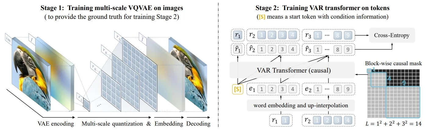
This completes the symbolic-to-visual generation pipeline. The transformer produces discrete codes that encode visual semantics and layout, while the VQ-VAE decoder renders them into photorealistic images.
Benefits of the VAR Design VAR’s architecture offers several advantages:
- 1.
- Spatial locality is preserved, avoiding the unnatural 1D flattening of images.
- 2.
- Inference is parallelized within each resolution, enabling fast generation.
- 3.
- Global structure is conditioned into finer details via multi-scale refinement.
- 4.
- Transformer capacity is efficiently used, since each level focuses on simpler sub-distributions.
Experimental Results: High-Quality Generation and Editing After training both the multi-scale VQ-VAE and the scale-aware transformer, the VAR model [635] demonstrates compelling performance across a range of image generation tasks. Notably, it achieves high visual fidelity on ImageNet [119] at resolutions up to \(512 \times 512\), and supports zero-shot editing — despite being trained with only unconditional or class-conditional supervision.
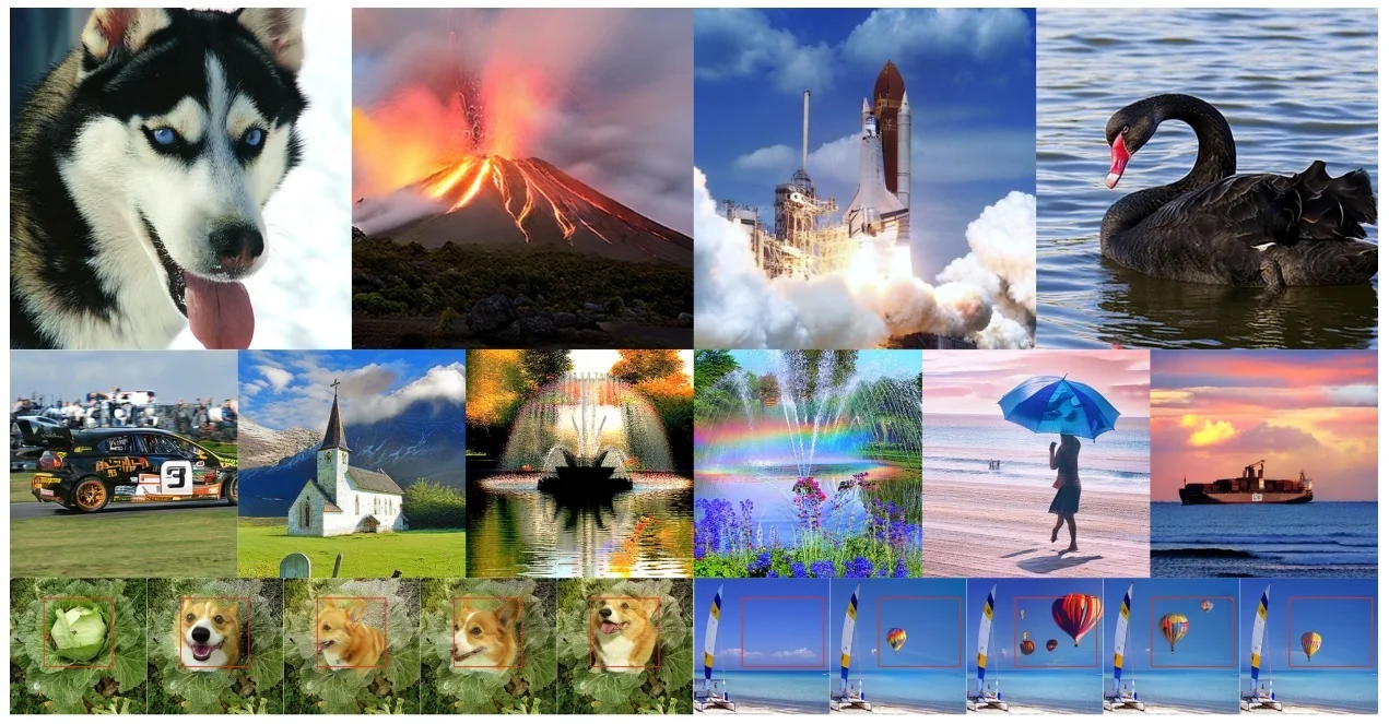
Generation Quality. VAR achieves state-of-the-art sample quality on the ImageNet-256 and ImageNet-512 benchmarks. Visually, its samples are both semantically rich and globally coherent — showcasing correct object structure, texture, and style. This is due to its coarse-to-fine generation mechanism: the transformer first predicts low-resolution structural layout via coarse token maps, then refines texture and details in subsequent finer maps, guided by the VQ-VAE decoder.
Zero-Shot Editing. The ability to modify image content without additional supervision is enabled by the discrete tokenization of the VQ-VAE and the structured generative pathway. In the bottom row of Figure 20.138, input images are embedded into VAR’s token space and selectively altered before decoding — showcasing realistic object transformations, viewpoint changes, and fine-grained edits, all without retraining the model.
Multi-Resolution Support. One key strength of VAR lies in its multi-resolution token maps, which naturally support different output scales. During inference, generation can stop at any intermediate resolution (e.g., \(64 \times 64\), \(128 \times 128\), etc.), offering flexible tradeoffs between quality and speed.
These results validate VAR’s autoregressive transformer as a strong alternative to diffusion- or GAN-based image generators. Its structured, scale-aware approach achieves both fidelity and controllability — setting the stage for broader multimodal extensions and architectural scaling.
Comparison with Other Generative Paradigms To contextualize the significance of VAR’s results, the authors benchmarked it against a wide spectrum of state-of-the-art generative models across four major paradigms: GANs, diffusion models, masked prediction models, and autoregressive (AR) transformers. The below table summarizes the comparison on the ImageNet \(256 \times 256\) class-conditional benchmark. Evaluation metrics include FID (lower is better), Inception Score (IS) (higher is better), and Precision/Recall for semantic and distributional quality, along with model size and inference cost (time).
| Type | Model | FID ↓ | IS ↑ | Pre ↑ | Rec ↑ | #Param | #Step | Time |
|---|---|---|---|---|---|---|---|---|
| GAN | BigGAN [52] | 6.95 | 224.5 | 0.89 | 0.38 | 112M | 1 | – |
| GAN | GigaGAN [284] | 3.45 | 225.5 | 0.84 | 0.61 | 569M | 1 | – |
| GAN | StyleGAN-XL [566] | 2.30 | 265.1 | 0.78 | 0.53 | 166M | 1 | 0.3 |
| Diff. | ADM [123] | 10.94 | 101.0 | 0.69 | 0.63 | 554M | 250 | 168 |
| Diff. | CDM [234] | 4.88 | 158.7 | – | – | 8100M | – | – |
| Diff. | LDM-4-G [548] | 3.60 | 247.7 | – | – | 400M | 250 | – |
| Diff. | DiT-XL/2 [492] | 2.27 | 278.2 | 0.83 | 0.57 | 675M | 250 | 45 |
| Diff. | L-DiT-3B [9] | 2.10 | 304.4 | 0.82 | 0.60 | 3.0B | 250 | >45 |
| Mask. | MaskGIT [77] | 6.18 | 182.1 | 0.80 | 0.51 | 227M | 8 | 0.5 |
| AR | VQGAN [149] | 15.78 | 74.3 | – | – | 1.4B | 256 | 24 |
| AR | ViTVQ-re [766] | 3.04 | 227.4 | – | – | 1.7B | 1024 | >24 |
| AR | RQTransformer [328] | 3.80 | 323.7 | – | – | 3.8B | 68 | 21 |
| VAR | VAR-d16 | 3.30 | 274.4 | 0.84 | 0.51 | 310M | 10 | 0.4 |
| VAR | VAR-d20 | 2.57 | 302.6 | 0.83 | 0.56 | 600M | 10 | 0.5 |
| VAR | VAR-d24 | 2.09 | 312.9 | 0.82 | 0.59 | 1.0B | 10 | 0.6 |
| VAR | VAR-d30 | 1.92 | 323.1 | 0.82 | 0.59 | 2.0B | 10 | 1.0 |
| VAR | VAR-d30-re | 1.73 | 350.2 | 0.82 | 0.60 | 2.0B | 10 | 1.0 |
Key Takeaways.
- VAR sets a new benchmark: It achieves the lowest FID (1.73) and the highest IS (350.2) of any model on ImageNet \(256 \times 256\), surpassing strong diffusion models like L-DiT [9] and GANs like StyleGAN-XL.
- Inference speed is dramatically faster: While diffusion models require hundreds of denoising steps (e.g., 250 for ADM, DiT), VAR completes generation in just 10 autoregressive steps — one per scale.
- Superior precision-recall tradeoff: VAR maintains high recall (0.60) without sacrificing precision, balancing diversity and realism in a way that standard AR models often fail to achieve.
Why VAR Outperforms Traditional VQ-VAE/VQ-GAN Autoregressive Models.
VAR demonstrates significant advantages over raster-scan VQ-based AR models such as VQ-GAN [149], ViT-VQGAN [766], and RQ-Transformer [328], by overcoming both architectural and theoretical limitations. These models typically flatten a 2D grid into a 1D token stream and predict each token sequentially—introducing inefficiencies and violating the natural spatial structure of images.
- Resolution of 2D-to-1D Flattening Issues. Flattening a 2D image into a 1D sequence for raster-order prediction introduces what the authors call a mathematical premises violation. Images are inherently 2D objects with bidirectional dependencies. Standard AR transformers, however, assume strict unidirectional causality, which conflicts with the actual structure of visual data. VAR resolves this mismatch via its next-scale prediction strategy, which operates hierarchically across scales, preserving spatial coherence and reducing unnecessary dependencies.
- Massive Reduction in Inference Cost. While traditional AR models require one autoregressive step per token (e.g., 256\(\times \)256 = 65,536 steps), VAR only needs \(K\) steps (typically \(K = 4\)–\(6\)), since each scale’s token map is generated in parallel. This reduction yields roughly \(O(N^2) \to O(K)\) sequential depth, improving inference speed by over 20\(\times \) in practice compared to VQ-GAN or ViTVQ baselines.
- Enhanced Scalability and Stability. Unlike earlier VQ-based AR models, which often suffer from training instability or limited scaling behavior, VAR exhibits smooth performance scaling with model size and compute. As shown in Table 20.13, the largest VAR variant surpasses both autoregressive and diffusion baselines at scale, demonstrating a power-law-like trend similar to that of large language models (LLMs).
Why VAR Avoids the Blurriness of Traditional VAEs
Standard VAEs often produce blurry images due to the averaging effect in continuous latent spaces and the use of simple L2 reconstruction loss. In contrast, VAR’s multi-scale VQ-VAE circumvents these issues using discrete representations and adversarial objectives:
- Quantized, Discrete Latents. The use of a discrete token space—learned via a shared codebook—eliminates interpolation-based blurriness. At each scale, the image is decomposed into a quantized map \({r}_k\), where tokens correspond to well-defined visual primitives rather than uncertain blends.
-
Residual-Style Encoder and Decoder. Each scale in the encoder captures residual detail not explained by the coarser maps, leading to a more structured and interpretable decomposition. The decoder sums contributions from all scales to reconstruct high-fidelity images with sharp contours and textures.
-
Perceptual and Adversarial Losses. VAR’s VQ-VAE is trained with a compound objective including:
- A perceptual loss \(\mathcal {L}_P\) (e.g., LPIPS) that compares image reconstructions in the feature space of a pretrained CNN like VGG, encouraging realism and sharpness over pixel-wise fidelity.
- An adversarial loss \(\mathcal {L}_G\) that penalizes visually implausible outputs via a GAN-style discriminator, pushing the generator to produce images indistinguishable from real data.
- Hierarchical Representation Enables Coherence. Unlike VQGANs that rely on a single token map, VAR’s hierarchical structure allows different scales to specialize: coarse layers ensure global layout, while fine layers refine details. This structured generation avoids both over-smoothing and oversharpening artifacts common in single-scale VAEs.
Taken together, these innovations allow VAR to combine the sharpness and semantic fidelity of GANs with the training stability and generative flexibility of VAEs—without inheriting their respective downsides.
Scaling Trends, Model Comparison, and Future Outlook VAR [635] demonstrates that coarse-to-fine autoregressive modeling is not only viable, but also highly competitive with, and in many respects superior to, both diffusion models and GANs. Its innovations in architectural design, inference efficiency, and training stability position it as a new standard for high-resolution image synthesis.
Scaling Efficiency and Sample Quality VAR exhibits favorable power-law scaling as model capacity increases. Across multiple variants (e.g., d16 to d30-re), both FID and Inception Score improve steadily, as shown in the below figure. The largest model, VAR-d30-re (2B parameters), achieves an FID of 1.73 and an IS of 350.2 on ImageNet \(256 \times 256\), outperforming L-DiT-3B and 7B, yet requiring only 10 autoregressive steps.
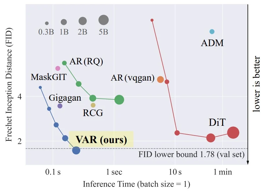
Comparison to Diffusion and Autoregressive Models As detailed in Table 20.13, VAR delivers best-in-class performance across fidelity, semantic consistency, and speed:
- Compared to diffusion models like ADM [123], DiT [492], and L-DiT [9], VAR matches or exceeds sample quality while reducing inference time by over 20×.
- Compared to GANs such as StyleGAN-XL [566], VAR achieves higher precision and recall, while being more stable and easier to scale.
- Most importantly, VAR outperforms previous autoregressive methods (e.g., VQGAN [149], ViT-VQGAN [766], and RQ-Transformer [328]) by resolving their core limitations — primarily the violation of spatial locality introduced by raster-scan decoding.
Qualitative Scaling Effects of VAR To further illustrate the benefits of architectural scaling, the authors created a figure that showcases qualitative samples from multiple VAR models trained under different model sizes \(N\) and compute budgets \(C\). The grid includes generations from 4 model sizes (e.g., VAR-d16, d20, d24, d30) at 3 different checkpoints during training. Each row corresponds to a specific class label from ImageNet [119], and each column highlights progression in visual quality with increasing capacity and training.
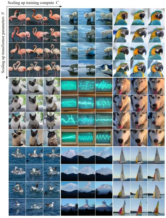
As visible in the figure, increased model scale and training compute systematically improve both semantic fidelity (correctness of object structure and attributes) and visual soundness (absence of artifacts, texture realism, and color consistency). For instance, the depiction of ”oscilloscope” and ”catamaran” transitions from ambiguous blobs in early-stage, small models to highly plausible, structurally accurate renderings in larger, well-trained variants.
These qualitative trends corroborate the quantitative findings in Figure 20.139 and Table 20.13, reinforcing that VAR inherits desirable scaling properties akin to large language models: more parameters and compute lead to predictable improvements in generative quality.
Limitations and Future Directions Despite its strengths, VAR still inherits certain limitations:
- Lack of native text conditioning: Unlike diffusion systems such as GLIDE or LDM, VAR has not yet been extended to text-to-image generation. Integrating cross-modal encoders (e.g., CLIP or T5) remains a promising avenue.
- Memory footprint: While more efficient than raster AR models, each scale in VAR still requires full-token parallel decoding, which may challenge memory limits for high-resolution outputs.
- Token discretization ceiling: The reliance on codebook-based representations may bottleneck expressiveness for fine-grained texture, unless dynamic or learned vocabularies are incorporated.
Nonetheless, VAR’s success opens up multiple promising research directions: extending the coarse-to-fine AR paradigm to multimodal transformers, integrating with prompt-based editing, and exploring learned topologies beyond rectangular grids. Its architectural clarity and empirical strength position it as a foundation for the next generation of efficient generative models.
Enrichment 20.11.12: DiT: Diffusion Transformers
Motivation and context Most high-performing diffusion models have used U-Net backbones that combine convolutional biases (locality, translation equivariance) with occasional attention for long-range interactions [123, 548]. The central question addressed by Diffusion Transformers (DiT) [492] is whether a pure Vision-Transformer denoiser operating in latent space can match or surpass U-Net diffusion when scaled. DiT answers in the affirmative: by patchifying VAE latents and processing tokens with transformer blocks modulated via adaptive LayerNorm (adaLN / adaLN-Zero), DiT exhibits clean scaling laws and achieves state-of-the-art ImageNet sample quality at competitive compute.
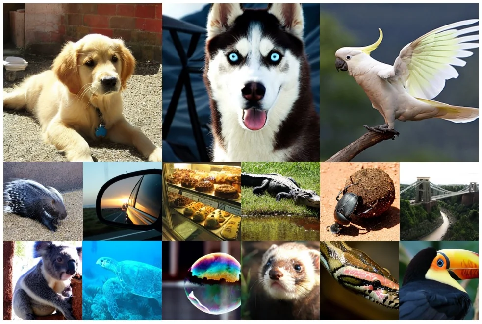
High-level overview DiT is a standard DDPM/latent-diffusion denoiser \(\epsilon _\theta \) that operates on VAE latents \(z_0=E(x)\in \mathbb {R}^{I\times I\times C}\) (e.g., \(I{=}32\), \(C{=}4\) for \(256^2\) images). With \(q(z_t\!\mid \!z_0)=\mathcal {N}\!\big (\sqrt {\bar \alpha _t}z_0,(1{-}\bar \alpha _t)I\big )\) and \(z_t=\sqrt {\bar \alpha _t}z_0+\sqrt {1{-}\bar \alpha _t}\,\epsilon \), the denoiser predicts \(\epsilon _\theta (z_t,t,c)\) (and a diagonal covariance) by minimizing the usual noise MSE. Class-conditional training uses classifier-free guidance at sampling time.
Why transformers? Intuition. Transformers have appeared repeatedly in earlier parts of this chapter: as attention submodules inside U-Nets, as text encoders, and even as full transformer U-Nets. What distinguishes DiT is the decision to use a pure ViT backbone directly on latent patch tokens, removing convolutional pyramids and skip connections entirely.
This shift yields several concrete benefits that are hard to obtain with U-Nets:
- Global-first context at every depth. Self-attention connects all tokens in all layers, coordinating layout and long-range dependencies continuously, rather than bottlenecking global context at specific resolutions as in U-Nets.
- Simpler, predictable scaling. DiT exposes two orthogonal knobs—backbone size (S/B/L/XL) and token count via patch size \(p\)—so quality tracks forward Gflops in a near-linear fashion. This clarity is difficult with U-Nets whose compute varies non-trivially with resolution and pyramid design.
- Uniform conditioning via normalization. Instead of injecting conditions via cross-attention at a few scales, DiT uses adaLN-style modulation in every block, giving cheap, global, step-aware control without the sequence-length overhead of cross-attention.
- Latent-space efficiency. Operating on VAE latents keeps sequence lengths manageable while retaining semantics. Convolutional U-Nets still pay per-pixel costs that grow with resolution, even in latent space.
In short, transformers are not merely “also used” here; the pure transformer backbone plus compute-centric scaling and adaLN-based conditioning together produce a qualitatively different, more scalable denoiser than a U-Net.
Method: architecture and components
Tokenization (patchify) of the latent. The noised latent \(z_t\in \mathbb {R}^{I\times I\times C}\) is split into non-overlapping \(p{\times }p{\times }C\) patches, each linearly projected to \(d\)-dim tokens with sine–cos positional embeddings. The sequence length is \(T=(I/p)^2\). Reducing \(p\) increases tokens (and Gflops) without changing parameters, acting as a clean compute knob.
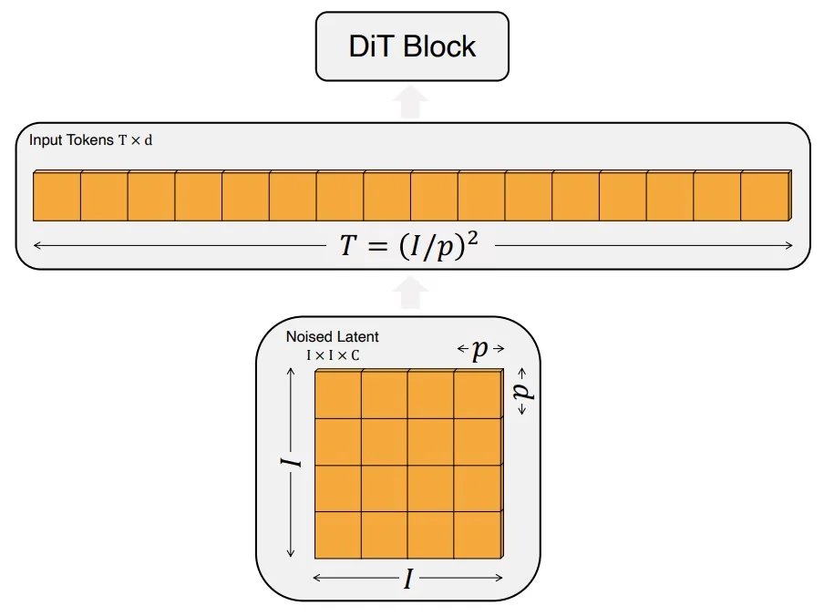
High-level overview: DiT as a transformer backbone for diffusion After tokenization, the task is to predict the additive noise on latent patches at diffusion timestep \(t\) (and, optionally, class/text label \(y\)). Diffusion Transformers (DiT) [492] replace the U-Net with a stack of transformer blocks that operate on the patch-token sequence: (i) patchify latents into tokens; (ii) transform them with \(N\) conditional blocks that inject \((t,y)\) at every depth; (iii) project tokens back to per-patch predictions (noise and optionally variance). The motivation is simple: self-attention offers global receptive fields and scales cleanly with depth/width; conditioning via adaptive normalization is cheap and pervasive.
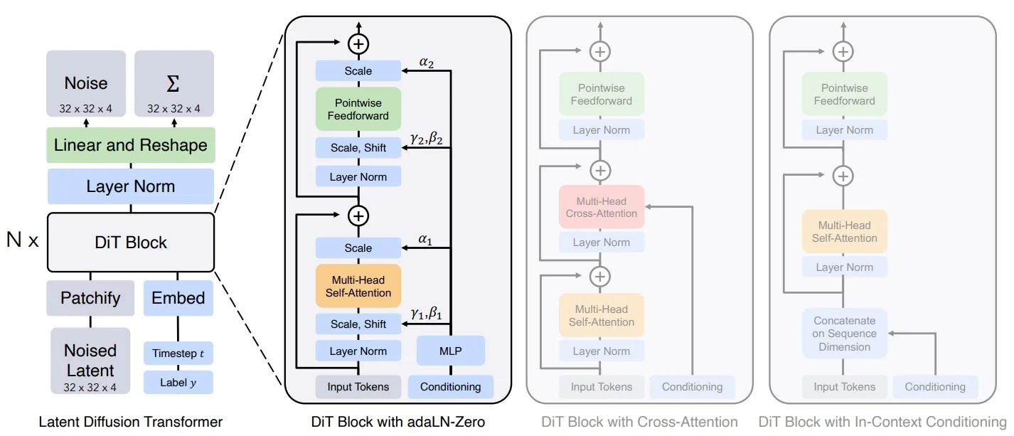
From AdaIN to adaLN: motivation and adaptation Adaptive normalization offers cheap, global control by modulating normalized activations with per-channel scale/shift. StyleGAN’s AdaIN Enrichment 20.6.1 applies \((\gamma ,\beta )\) (from a style code) after InstanceNorm in convnets, broadcasting “style” through every layer with negligible overhead. DiT carries this idea to transformers and diffusion by:
- Swapping InstanceNorm on feature maps for LayerNorm on token embeddings.
- Replacing style latents with diffusion timestep \(t\) and label/text \(y\) as the condition.
- Adding zero-initialized residual gates so very deep stacks start near identity and “open” gradually (stability under heavy noise).
This preserves AdaIN’s low-cost, layer-wise control while fitting the sequence setting and the iterative denoising objective.
DiT block: adaLN and the adaLN-Zero variant The DiT backbone is a sequential stack of \(N\) standard Pre-LN transformer blocks. Each block consumes a token sequence \(X\in \mathbb {R}^{L\times d}\) and applies \[ \mbox{(i) LN} \rightarrow \mbox{MHSA} \rightarrow \mbox{residual},\qquad \mbox{(ii) LN} \rightarrow \mbox{MLP} \rightarrow \mbox{residual}. \] Why this works. MHSA lets every latent patch-token attend to all others, building global spatial coherence; the MLP adds channel-wise capacity after attention has mixed information. Conditioning the LayerNorms lets \(t,y\) shape what MHSA/MLP see—cheaply and pervasively—so early steps favor coarse denoising and later steps focus on fine details.
How conditioning is produced (per-block MLPs, as in DiT). Embed the diffusion timestep and label/text and concatenate to form \(c=\mathrm {Embed}(t,y)\in \mathbb {R}^e\) (sinusoidal \(t\)-embed + learned \(y\)-embed). Each transformer block \(i\) owns a tiny modulation MLP \(g_i:\mathbb {R}^e\!\to \!\mathbb {R}^{6d}\) that outputs six \(d\)-vectors \[ (\gamma _{1,i},\beta _{1,i},\alpha _{1,i},\gamma _{2,i},\beta _{2,i},\alpha _{2,i}) \;=\; g_i(c), \] one triplet for the attention branch (\(k{=}1\)) and one for the MLP branch (\(k{=}2\)). This gives shallow and deep layers different “views” of \((t,y)\) with negligible parameter cost.2
adaLN (adaptive LayerNorm). At each Pre-LN site (before self-attention and before the MLP), replace vanilla LayerNorm by a condition-dependent affine transform: \[ \mathrm {adaLN}_k(X;c)\;=\;\gamma _{k,i}(c)\odot \mathrm {LN}(X)\;+\;\beta _{k,i}(c),\qquad k\in \{1,2\}. \] This injects \((t,y)\) everywhere using only elementwise operations, so the subsequent computations see features already bent toward the current diffusion step and class.
adaLN-Zero (the variant used in practice). DiT’s best-performing blocks add gates on the two residual branches via \(\alpha _{1,i}(c),\alpha _{2,i}(c)\) that are zero-initialized. With \(X\!\in \!\mathbb {R}^{L\times d}\), a full block computes \[ \begin {aligned} Z_1 &= \mathrm {adaLN}_1(X;c), \qquad H \;=\; \mathrm {SelfAttn}(Z_1), \qquad U \;=\; X \;+\; \alpha _{1,i}(c)\odot H,\\ Z_2 &= \mathrm {adaLN}_2(U;c), \qquad M \;=\; \mathrm {MLP}(Z_2), \qquad Y \;=\; U \;+\; \alpha _{2,i}(c)\odot M. \end {aligned} \] Here \(\mathrm {SelfAttn}\) is the standard multi-head scaled dot-product self-attention (MHSA); some figures abbreviate it as “self-attn”. Self-attention lets every token attend to every other (global communication); the multi-head factorization runs several attentions in parallel so different heads can specialize (e.g., shape vs. texture), then concatenates and projects them back to \(d\). Zero-initialized gates make the whole stack start near identity (\(Y\!\approx \!X\)), preventing early instabilities on very noisy inputs; during training the model learns where to “open” attention/MLP paths. Empirically, adaLN-Zero is the variant used for final models; plain adaLN appears mainly in ablations.
Head and parameterization After the final LayerNorm, a linear head maps each token to \(p{\times }p{\times }(2C)\) values (per patch; commonly \(p{=}1\)), then reshapes to the latent grid. The first \(C\) channels parameterize the predicted noise; the remaining \(C\) optionally parameterize a diagonal variance. Across \(T\) denoising steps, DiT iteratively predicts and removes noise to recover a clean latent \(x_0\); a pretrained VAE decoder then converts \(x_0\) to pixels (e.g., \(256{\times }256\) RGB). Intuitively: MHSA builds global structure across patches, the MLP refines channel-wise details, adaLN/Zero injects timestep/class signals at every depth, and the head “de-tokenizes” back to a spatial latent that the VAE upsamples to the final image.
Conditioning and guidance The condition \(c\) is the concatenation of timestep and class/text embeddings. Classifier-free guidance is enabled by randomly replacing the label with a learned “null” embedding during training. At inference, combine unconditional and conditional predictions as \[ \tilde {\epsilon }\;=\;\epsilon _{\emptyset }\;+\;s\,(\epsilon _{y}-\epsilon _{\emptyset }),\qquad s>1, \] steering samples toward the target class/text. Among conditioning routes (in-context tokens, cross-attention, adaLN, adaLN-Zero), adaLN-Zero consistently converges fastest and achieves the best FID with negligible overhead; cross-attention is more flexible for long text but typically adds \(\sim 15\%\) compute.
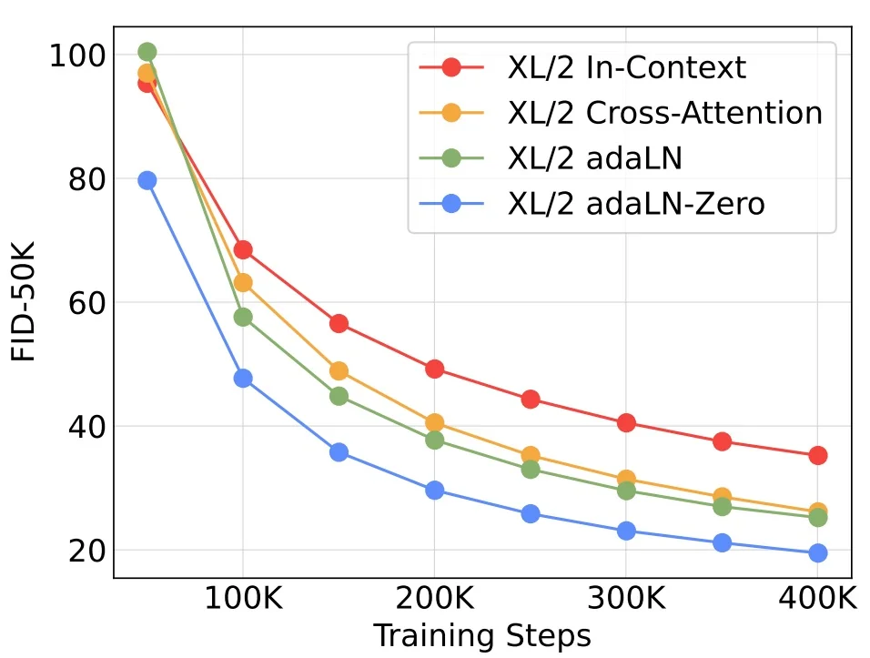
Training objective and setup DiT trains end-to-end in latent space with the standard denoising objective. For VAE-encoded images \(x_0\), noise \(\epsilon \!\sim \!\mathcal {N}(0,I)\), timestep \(t\), and condition \(y\), \[ \mathcal {L} \;=\; \mathbb {E}_{x_0,\epsilon ,t,y}\Big [\;\big \|\epsilon \;-\; \hat {\epsilon }_\theta (x_t,t,y)\big \|_2^2\;\Big ], \quad x_t \;=\; \sqrt {\bar {\alpha }_t}\,x_0 \;+\; \sqrt {1-\bar {\alpha }_t}\,\epsilon . \] Classifier-free guidance is enabled by dropping \(y\) with some probability during training and learning a null embedding. In practice, AdamW with cosine LR decay and a brief warm-up are used; adaLN-Zero’s identity start helps avoid early instabilities in deep attention stacks while maintaining the capacity benefits of transformers.
Experiments and ablations
Scaling and SOTA comparisons. Compute-centric scaling is the core story. DiT exposes two orthogonal axes: backbone size (S/B/L/XL) and token count via patch size (\(p\!\in \!\{8,4,2\}\)). Increasing either axis improves FID at fixed training steps; the best results combine large backbones and small patches.
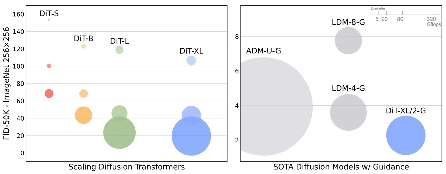
Training-time scaling trends. Holding \(p\) fixed and increasing backbone (S\(\rightarrow \)XL) lowers FID throughout training; holding backbone fixed and decreasing \(p\) (more tokens) also lowers FID. The separation between curves indicates robust compute-to-quality scaling across 12 configurations.
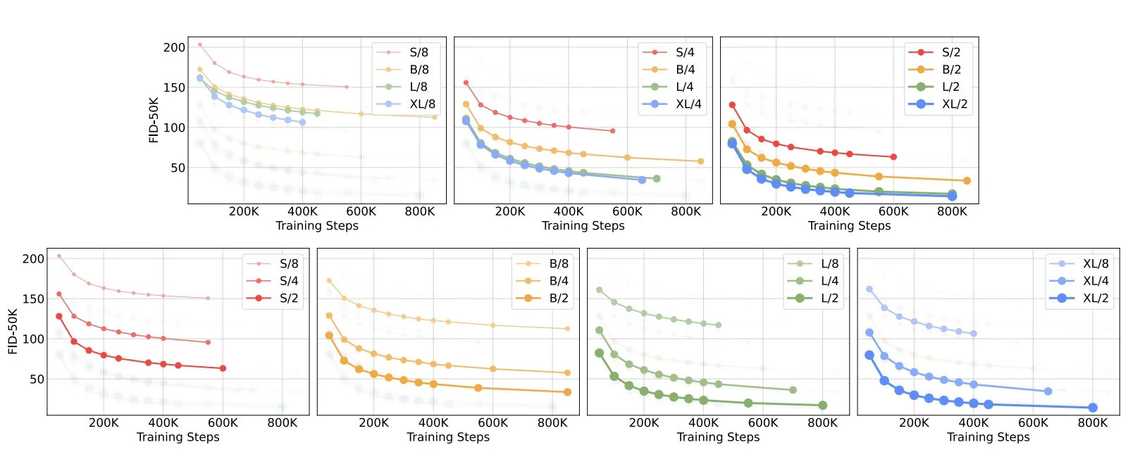
Qualitative scaling: more flops \(\rightarrow \) better images. A large grid sampled at 400K steps from the same noise and label shows that increasing transformer Gflops—either via larger backbones or more tokens—improves visual fidelity. Left-to-right increases backbone size; top-to-bottom decreases patch size (more tokens).
Gflops predict FID. Across all 12 DiTs at 400K steps, transformer forward Gflops strongly correlates with FID (reported correlation \(\approx \!-0.93\)). This metric predicts quality better than parameter count and makes design trade-offs explicit.
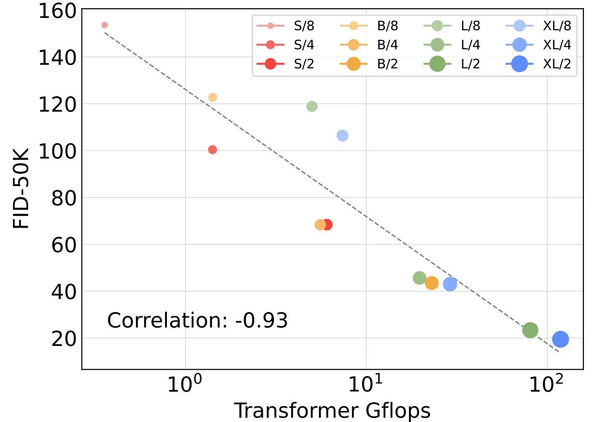
Total training compute vs. FID. Plotting FID against total training compute shows smooth, near power-law improvements. Larger models form a lower envelope: for the same train compute, bigger models reach better FID than smaller ones trained longer.
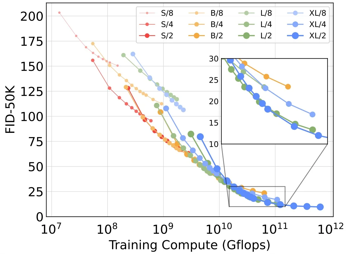
Sampling compute cannot replace model compute. Increasing denoising steps improves quality for each model, but small models cannot catch large ones even with more sampling steps (higher inference Gflops). For a fixed sampling budget, it is typically better to deploy a larger DiT at fewer steps than a smaller DiT at many steps.
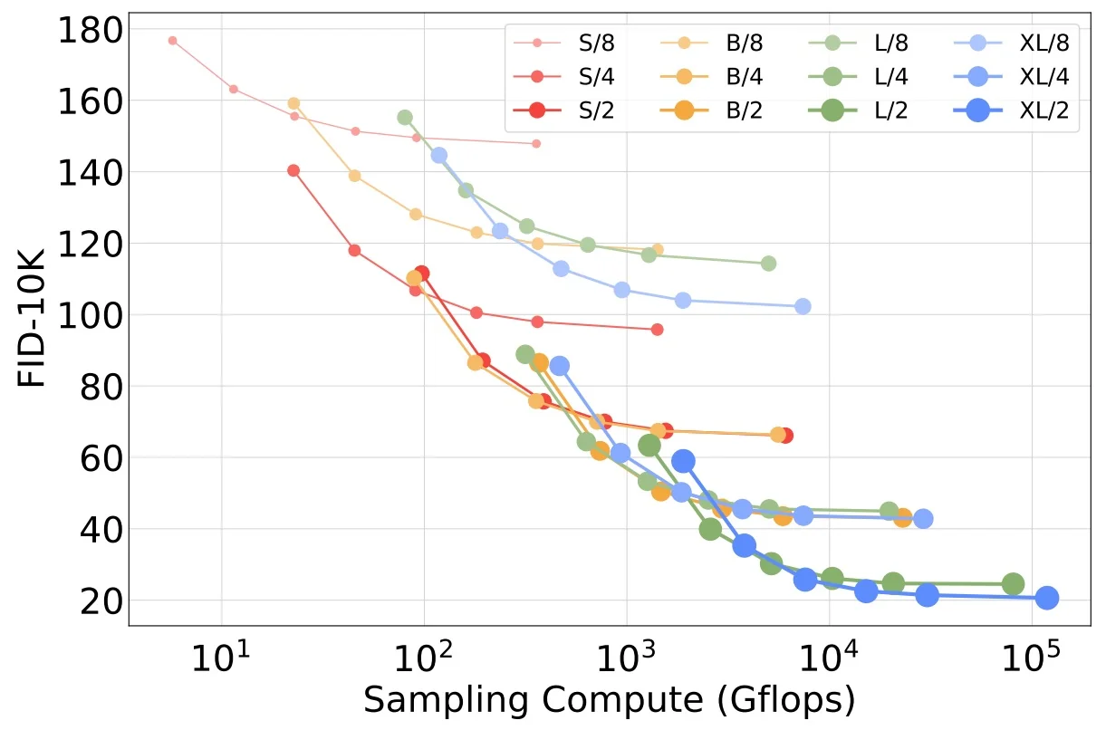
Benchmark summary (ImageNet 256/512). On ImageNet-256, DiT-XL/2 with classifier-free guidance (scale \(\approx \)1.5) attains FID \(\approx \) 2.27, sFID \(\approx \) 4.60, and IS \(\approx \) 278, exceeding LDM and ADM variants. At 512, DiT maintains strong results with FID \(\approx \) 3.04. Precision/Recall indicate balanced fidelity/diversity relative to GAN and diffusion baselines. (Exact tables are in [492]; summarized here for brevity.)
What changed vs. Stable Diffusion and why it matters
- Backbone. U-Net (ResNet blocks + spatial attention at select scales) \(\Rightarrow \) pure ViT over patch tokens. DiT’s global-first attention coordinates layout at all depths; no hand-crafted multi-scale pyramid or skip connections are required.
- Conditioning. Cross-attention to text (costly, sequence-length dependent) \(\Rightarrow \) adaLN / adaLN-Zero (cheap, global, step-aware). This adapts AdaIN-style modulation (Enrichment 20.6.1) to LayerNorm, distributing conditioning throughout the network with near-zero overhead and superior FID (see Figure 20.144).
- Scaling lens. Params and resolution-dependent conv costs \(\Rightarrow \) forward Gflops as the primary metric. As shown in Figure 20.148, Gflops strongly predicts FID and guides trade-offs between model size and token count.
-
Compute knobs. Channel/width heuristics and UNet depth \(\Rightarrow \) orthogonal knobs (backbone size S/B/L/XL and patch size \(p\)). Figures 20.145–20.147 demonstrate monotonic quality gains along both axes.
- Variance head. DiT’s head predicts noise and a diagonal covariance per spatial location, enabling variance-aware denoising in latent space.
Outcome. At similar or lower compute, DiT matches or surpasses U-Net diffusion on ImageNet, and scales predictably (quantitatively in Figure 20.148, Figure 20.149; qualitatively in Figure 20.147).
Relation to prior and follow-ups AdaIN-based control in StyleGAN1 (Enrichment 20.6.1) motivated normalization-as-conditioning; DiT shows a transformer-native realization (adaLN-Zero). Subsequent work such as L-DiT [9] scales DiT further in latent space, reporting even stronger ImageNet results. DiT complements latent U-Nets [548]: both benefit from classifier-free guidance and VAE latents, but DiT offers LLM-like scaling and a simpler global-context story.
Limitations and future work
- Memory/latency at small \(p\). Reducing \(p\) increases tokens \(T\) and attention memory quadratically in \(I\); efficient attention, sparse routing, or hierarchical tokenization are promising.
- Inductive bias. Removing convolutions removes explicit translation equivariance and pyramids; hybrid conv–transformer blocks or relative position biases may improve data efficiency.
- Long-sequence conditioning. Cross-attention for long text is flexible but adds compute; extending adaLN-style modulation to long sequences or hybridizing with lightweight cross-attention is an open avenue.
Practical recipe Train in latent space with a strong VAE. Pick DiT-B/L/XL by budget. Start at \(p{=}4\), drop to \(p{=}2\) if memory allows. Expect monotonic FID gains by increasing backbone size and tokens (Figure 20.146, Figure 20.148). Prefer a larger DiT with fewer steps over a smaller DiT with many steps for a fixed sampling budget (Figure 20.150).
Enrichment 20.11.13: Rectified Flow (RF): Straightening the Global Vector Field
The Straight-Line Paradox: Why Straight Training Data Yields Curved Inference In Affine Flow Matching, we train on pairs \((x_0, x_1)\) connected by perfect straight lines: \[ x_t = (1-t)x_0 + t x_1. \] Since every single training trajectory is a straight line, one might intuitively expect the learned model to also generate straight lines. This is incorrect.
The Source of Confusion: Crossing Paths Create Conflicting Gradients. To understand why the flow curves, we must look at what happens at a single point in space where training trajectories intersect.
- 1.
- The Setup (Training Data): Imagine the training data as thousands of straight strings connecting noise to images. Because we paired them randomly, these strings form a dense, tangled web. In high dimensions, millions of these strings cross through the same spatial regions.
- 2.
- The Conflict (At Point \(x\)): Consider a specific point \(x\) in the middle of the
flow.
- String A passes through \(x\) heading straight to Image A (North).
- String B passes through \(x\) heading straight to Image B (East).
During training, the network visits \(x\) multiple times. Sometimes it is told ”Target = North”, other times ”Target = East”.
- 3.
- The Resolution (Conditional Expectation): The neural network is a function \(v(x, t)\). It cannot output ”North” and ”East” simultaneously for the same input. To minimize the squared error for both cases, it learns the average vector: Northeast.
Why the Inference Trajectory Curves (Step-by-Step): Now, consider the ODE solver trying to generate a sample during inference. Crucially, the solver only knows the noise \(x_0\); it does not know which target image it ”should” go to. It must rely entirely on the network’s learned field at its current position.
- Step 1 (The Compromise): The solver arrives at a point \(x\) where two training paths crossed: one heading to Target A (North) and one to Target B (East). Since the network learned the average, it tells the solver: ”Go Northeast”.
- Step 2 (The Drift): The solver takes a step Northeast. By doing so, it physically moves away from the straight line pointing to Target A, and away from the straight line pointing to Target B. It drifts into a region between them that neither training particle visited.
- Step 3 (The Turn): In this new ”no-man’s-land”, the solver encounters a different set of crossing paths (e.g., paths heading North and West). The network computes a new local average based on these new influences, causing the solver to change direction.
- Result: Instead of following a single straight line to a specific destination, the solver is continuously steered by a shifting consensus of all nearby paths. This constant re-adjustment creates a smooth curve.
Straight Training Paths + Crossings = Curved Average Flow.
Consequence. Because the learned vector field is curved, simple ODE solvers (like Euler) introduce large truncation errors unless the step size is very small. To enable fast, few-step generation, we must untangle the web so that paths do not cross—this is the goal of Rectified Flow.
Rectified Flow: From ”Ghost” Paths to ”Fluid” Flow To understand Rectified Flow, we must separate (i) the training construction that produces supervision targets from (ii) the ODE that the trained model actually defines at inference.
- 1.
- The interpolation process (\(X_t\)): the ”ghost” world. During training, we sample a coupling \((X_0,X_1)\) between \(\pi _0\) (noise) and \(\pi _1\) (data), and define straight chords \[ X_t = (1-t)X_0 + tX_1, \qquad \dot {X}_t = X_1 - X_0. \] With an independent (random) coupling, many chords pass through the same location \(x\) at the same time \(t\) but with different directions (e.g., one chord ”wants” to go North, another wants to go East). This produces conflicting gradients: the regressor cannot output multiple directions at the same input \((x,t)\), so (under squared loss) it learns the conditional average.
- 2.
- The rectified ODE (\(Z_t\)): the ”fluid” world. After training, we discard the individual ghost chords and keep only the learned global field \(v_\theta (x,t)\). Inference samples are generated by integrating the ODE \[ \frac {d}{dt} Z_t = v_\theta (Z_t,t), \qquad Z_0 \sim \pi _0. \] Because a deterministic ODE assigns a single velocity to every state \((x,t)\), its trajectories are non-crossing (given standard regularity / uniqueness conditions): if two particles ever coincide at the same \((x,t)\), they must share the same instantaneous velocity and thus move together thereafter.
The Guarantee: Why the ”Average” Path is the Correct Path A natural concern is that the ODE paths \(Z_t\) are not the original straight ghost chords \(X_t\). Does this discrepancy break correctness?
No: the conditional-expectation field preserves marginals. If we define the regression-optimal field \[ v^*(x,t) = \mathbb {E}\!\left [\dot {X}_t \mid X_t = x\right ] = \mathbb {E}\!\left [X_1 - X_0 \mid X_t = x\right ], \] then the probability flow induced by the continuity equation implies that the ODE driven by \(v^*\) reproduces the same time-marginal distributions as the interpolation process: \[ \mathrm {Law}(Z_t) \equiv \mathrm {Law}(X_t), \quad \forall t \in [0,1]. \] Intuitively: in the ghost world, straight walkers can pass through each other; in the fluid world, solid particles must swerve and swap destinations to avoid collisions. Individual identities change, but a blurred density snapshot at time \(t\) looks the same in both worlds.
This marginal-preservation viewpoint is central in Rectified Flow and Flow Matching analyses [389, 373].
The Catch. Although \(Z_t\) is correct, it is often curved (because it follows local averages in a crowded field), so coarse discretizations incur large truncation error. This is why naive few-step Euler sampling can fail even when the training targets were straight.
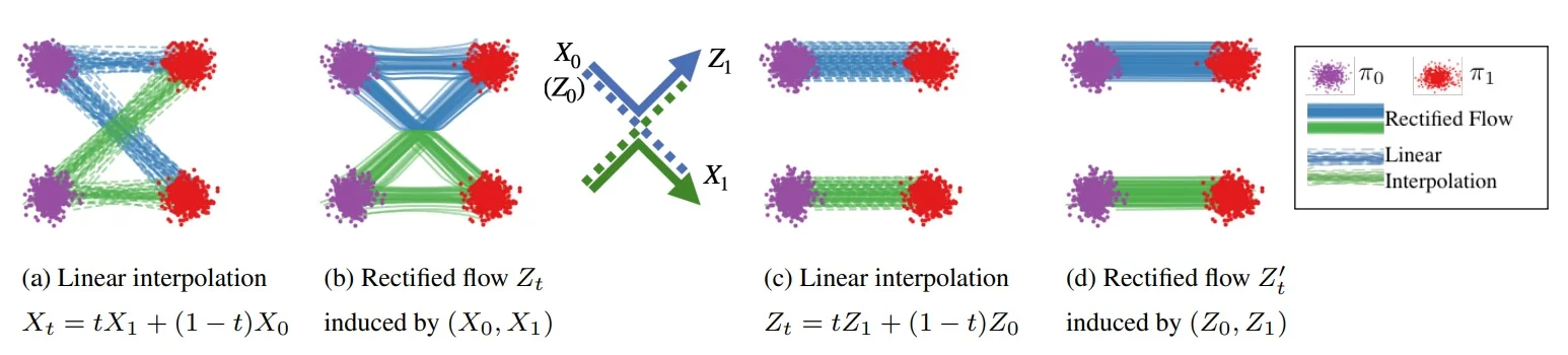
The Solution: Reflow as ”Coupling Repair” (Sorting + Wire Swapping) Rectified Flow’s key move is to use the current ODE to produce a better coupling. Integrate the rectified ODE from many starting noises \(Z_0 \sim \pi _0\) and record endpoints \(Z_1\). The resulting pairs \((Z_0,Z_1)\) form a new coupling between \(\pi _0\) and \(\pi _1\) that is causally linked by a non-crossing flow.
- Sorting intuition. The ODE acts like a “tangle-remover”: nearby starting points move together and end at compatible locations, instead of randomly aiming at far-apart targets that force many crossings.
- Wire swapping intuition (triangle inequality). Consider two crossed assignments (an “X”): \(A \mapsto D\) and \(B \mapsto C\). After rectification, the effective assignment becomes uncrossed (“\(=\)”): \(A \mapsto C\) and \(B \mapsto D\). Geometrically, uncrossing shortens total path length: \[ |AC| + |BD| \le |AD| + |BC|. \] This is the simplest picture of why rectification reduces transport complexity (and, in the paper, why convex transport costs do not increase).
- Straight-line test. Reflow still trains on straight chords between endpoints, but because the endpoints are now “sorted” by a non-crossing flow, those chords are far less likely to create severe, contradictory crossings than the original random pairing.
Recursive Reflow: Iterative Straightening Why do we repeat this process? If the ODE in Step 1 already ”untangles” the paths, why isn’t the result perfectly straight immediately?
The answer lies in the subtle difference between the Curved Trajectory (ODE) and the Straight Training Target (Chord).
- The ODE (\(v_k\)) is Non-Crossing but Curved: The solver prevents collisions by steering particles around each other. Think of it as a river flowing around obstacles: the water doesn’t cross itself, but it winds and curves.
- The New Target (Straight Line) May Still Cross: When we train the next model (\(v_{k+1}\)), we supervise it with the straight line connecting the start (\(Z_0\)) and the end (\(Z_1\)). Even if the curved ODE paths didn’t intersect, the straight lines connecting their endpoints might still overlap or form an ”X”.
- The Consequence: If the straight targets cross, the new model \(v_{k+1}\) receives conflicting gradients at the intersection. It resolves this by learning the average, which re-introduces curvature.
Step-by-Step Procedure:
- 1.
- Train Model \(v_k\) (The Curve): Train the velocity field \(v_k\) on the current dataset pairs \((Z^k_0, Z^k_1)\). Status: The model learns a valid flow, but the trajectories are likely curved because the training chords crossed.
- 2.
- Generate New Targets (The Reflow Step): For every fixed noise sample \(Z_0\) (anchored), run the ODE solver using the current model \(v_k\) to find its destination: \[ Z_1^{\mbox{new}} = \mbox{ODE}[v_k](Z_0). \] Note: The solver follows the curved, non-crossing path to find the ”natural” destination for this noise.
- 3.
- Update the Coupling (The Shortcut): Create the dataset for round \(k+1\). We keep the same starting noise \(Z_0\) but assign the new endpoints: \[ (Z^{k+1}_0, Z^{k+1}_1) = (Z_0, Z_1^{\mbox{new}}). \]
- 4.
- Result (Convergence): The new pairs are connected by a ”tighter” coupling. Since the endpoints are now sorted by the ODE, the straight lines connecting them cross far less frequently. As \(k \to \infty \), the coupling converges to a Monge Map. In this limit, the straight lines themselves do not cross, meaning the learned model \(v_\infty \) becomes a perfect straight flow, allowing for 1-step generation.
Why Reflow Unlocks One-Step Sampling The ultimate benefit of this straightening is numerical efficiency. Standard ODE solvers (like Euler) approximate a trajectory by taking small steps along the tangent. The error in this approximation (truncation error) is proportional to the curvature (the second derivative of the path).
- Curved Path: \(\ddot {x}_t \neq 0\). The solver drifts off the manifold unless the step size \(dt\) is tiny.
- Straight Path: \(\ddot {x}_t = 0\). The tangent at the start points exactly to the destination.
Because Reflow drives trajectories toward perfect straight lines, the curvature vanishes. In the limit, the Euler update becomes exact even for a single giant step (\(dt=1\)): \[ x_1 \;\approx \; x_0 + v_\theta (x_0,0). \] This is the theoretical foundation for InstaFlow and other ”turbo” distillation methods: they transform the complex diffusion process into a simple, straight-line velocity prediction that requires no integration loop.
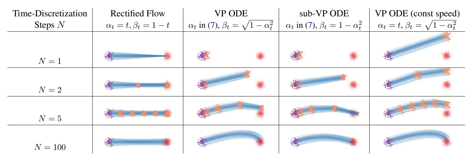
Practical Recipe: The Reflow Loop To implement Rectified Flow, we treat the generation process as a recursive loop where the model improves its own training data.
- 1.
- Step 1: The Base Model (1-Rectified)
- Train a velocity field \(v_1\) on standard independent pairs \((x_0, x_1) \sim \pi _0 \times \pi _1\).
- Result: The model learns to transport noise to data, but via curved, crossing paths (the ”average” flow).
- 2.
- Step 2: Dataset Generation (Reflow)
- Sample a large batch of noise \(z_0 \sim \pi _0\).
- Solve the ODE using \(v_1\) to generate corresponding endpoints: \(z_1 = \mbox{ODE}[v_1](z_0)\).
- Store the pairs \(\mathcal {D}_{\mbox{new}} = \{(z_0, z_1)\}\). These pairs are causally linked by a valid, non-crossing flow.
- 3.
- Step 3: The Straightened Model (2-Rectified)
- Train a new velocity field \(v_2\) on \(\mathcal {D}_{\mbox{new}}\) using the same linear interpolation objective.
- Result: Since the pairs \((z_0, z_1)\) are already connected by a valid flow, the straight line between them is a highly accurate approximation. \(v_2\) is significantly straighter and faster to simulate.
Takeaway The key insight of Rectified Flow is that straight training targets do not guarantee a straight global flow—unless the data coupling is perfect.
- 1-Rectified Flow makes trajectories straight conditionally (for each specific pair), but global crossings induce curvature.
- 2-Rectified Flow makes trajectories straight globally by repairing the coupling. It ”uncrosses the wires”, systematically reducing transport cost and curvature.
This straightening is what unlocks the next major advance: distilling these paths into a single step.
Enrichment 20.11.14: Stable Diffusion 3: Scaling Rectified Flow
Motivation: Addressing Architectural, Training, and Data Limitations Prior to Stable Diffusion 3 (SD3), the state-of-the-art was largely defined by models like SDXL [496], which relied on U-Net backbones that showed diminishing returns under further scaling. Concurrently, while standard diffusion models achieved strong visual quality, their probability trajectories involved significant amounts of curvature, requiring many ODE solver steps and making fast inference difficult [150]. Furthermore, as highlighted by DALL-E 3 [42], even large-scale visual backbones struggled with complex prompt adherence due to the simplistic, subject-focused nature of human-generated training captions.
To address these limitations, the SD3 recipe [150] replaces the U-Net backbone and standard diffusion formulation with four key upgrades:
- extbfMathematical Shift (Tailored Rectified Flow): To enable fast inference with fewer sampling steps, SD3 adopts Rectified Flow (RF) with straight generation paths [389, 373]. Because standard RF trains uniformly and underweights the perceptually difficult intermediate timesteps, SD3 introduces a Logit-Normal sampling schedule to bias training towards these critical transition regions.
- Architectural Shift (MM-DiT): Recognizing that U-Nets were no longer scaling efficiently, SD3 replaces them with the Multimodal Diffusion Transformer (MM-DiT). By utilizing dual independent weight streams that only interact during attention, it prevents text and image tokens from competing for a single representational space.
- Data Shift (Synthetic Captioning): Following the paradigm established by DALL-E 3 [42], SD3 incorporates highly detailed synthetic captions generated by Vision-Language Models (VLMs) alongside original captions, drastically improving the model’s spatial reasoning and complex prompt comprehension.
- High-Resolution Scaling Stability: Scaling continuous-time transformers to 8 billion parameters introduces attention entropy instabilities during mixed-precision training. SD3 resolves this via QK-normalization and applies resolution-dependent timestep shifting to maintain consistent generative difficulty across resolutions.
By addressing these practical bottlenecks, SD3 successfully scales Rectified Flow transformers up to 8B parameters, achieving strong improvements in prompt adherence, typography generation, and overall visual fidelity [150].
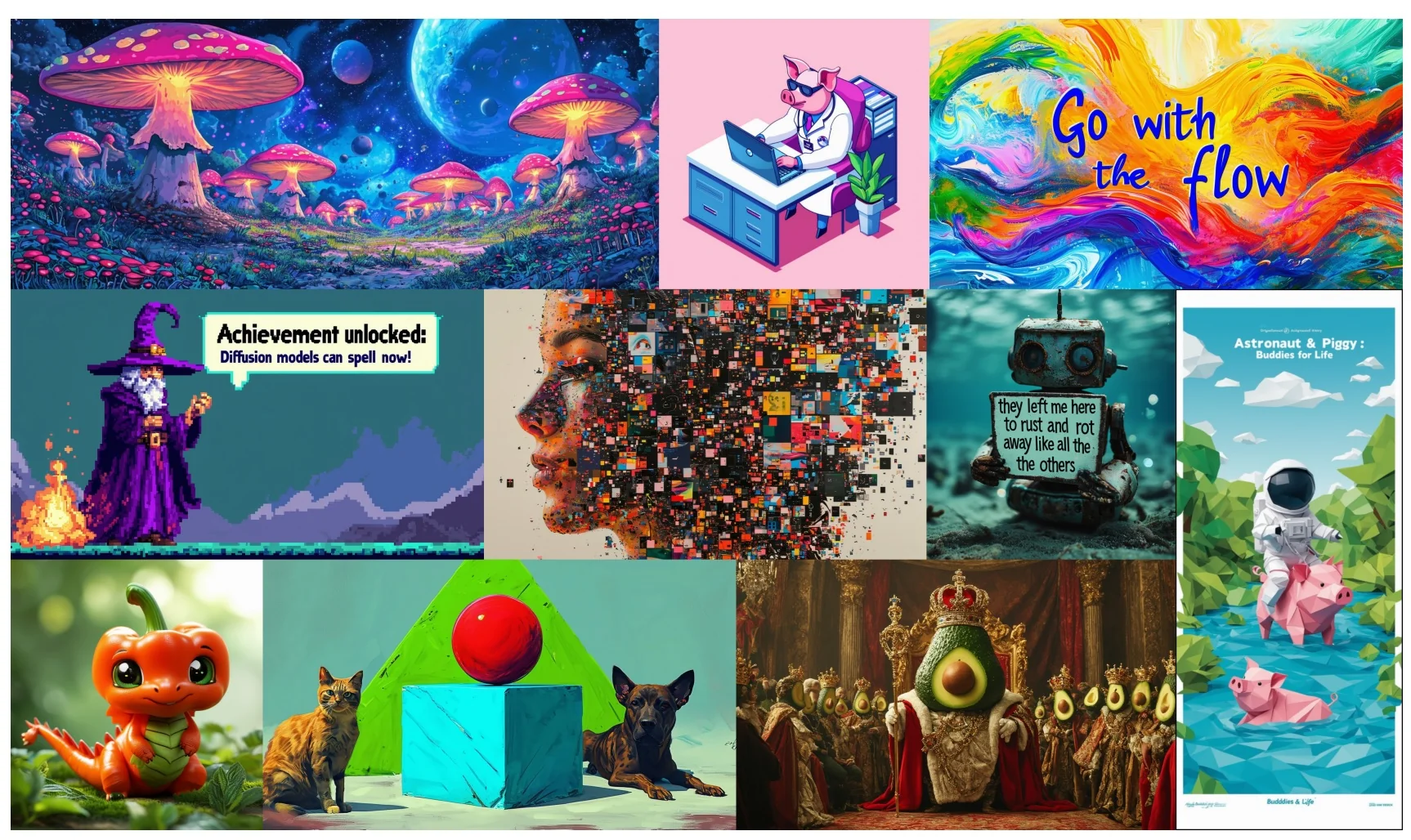
1. Rectified Flow as Simulation-Free Flow Matching At its mathematical core, SD3 adopts the continuous-time framework of simulation-free Flow Matching. Instead of relying on traditional diffusion formulations, it explicitly defines a forward probability path between the data distribution \(p_0\) and a standard normal noise distribution \(p_1=\mathcal {N}(0,I)\). The model’s objective is to learn the velocity vector field that transports mass along this path. Because the target velocity of this path is mathematically predefined, the network can be trained via simple regression without ever backpropagating through a computationally expensive ODE solver [373, 150].
Specifically, Rectified Flow (RF) enforces the simplest possible geometry—a straight line between data and noise:
\begin {equation} z_t = (1-t)\,x_0 + t\,\epsilon , \qquad x_0\sim p_0,\;\epsilon \sim \mathcal {N}(0,I),\;t\in [0,1]. \label {eq:chapter20_sd3_rf_path} \end {equation}
By taking the time derivative of this interpolation, Conditional Flow Matching yields a remarkably tractable regression target: the neural network must simply predict the constant velocity, \(\epsilon - x_0\), required to traverse this straight line [150].
While geometrically elegant, this straight path introduces a hidden optimization challenge. A unified mathematical analysis by [150] reveals that, when translated into the standard diffusion noise-prediction framework, standard RF implicitly applies a characteristic timestep weighting:
\begin {equation} w_t^{\mathrm {RF}}=\frac {t}{1-t}. \label {eq:chapter20_sd3_rf_weight} \end {equation}
This formulation exposes a critical flaw in naïve RF training. If timesteps \(t\) are sampled uniformly from \(\mathcal {U}(0,1)\) during training, the network dedicates equal capacity to every phase of the trajectory.
However, predicting the target velocity is mathematically trivial at the extremes (\(t \approx 0\) or \(t \approx 1\)) and profoundly difficult in the mid-range noise scales. Uniform sampling starves the network of training signals right in the middle of the trajectory—the exact transitional phase where the model must resolve abstract noise into coherent semantic structures.
2. Tailored SNR Samplers: Biasing Training to the Hard Timesteps To solve the capacity starvation problem identified in uniform sampling, the central methodological contribution of SD3 is to explicitly reshape the timestep sampling distribution during Rectified Flow training [150].
Intuitively, predicting the constant velocity target \(\epsilon -x_0\) is trivial at the extremes. Near \(t \approx 1\) (almost pure noise), the optimal velocity prediction collapses to the negative mean of the data distribution, since \(x_0\) averages out. Near \(t \approx 0\) (almost clean data), the optimal prediction collapses to the mean of the noise distribution (approximately zero), since \(\epsilon \) averages out. The true generative bottleneck lies in the middle, where the model must resolve ambiguous, partially structured signals into coherent semantic features.
Formally, when a diffusion model trains, it randomly selects a timestep \(t \in [0,1]\) for each image in the batch. Standard Rectified Flow draws this \(t\) from a uniform distribution, meaning the network has an equal probability of landing on any timestep. Consequently, it spends just as much compute time learning the trivial extremes as it does struggling with the difficult middle.
To fix this, [150] replaces the uniform distribution with a custom density \(\pi (t)\)—a targeted probability curve that essentially rigs the random number generator to pick specific timesteps more frequently. Mathematically, drawing samples from a custom probability density \(\pi (t)\) is equivalent to calculating the expected loss under a uniform distribution but explicitly multiplying the loss by \(\pi (t)\). Thus, the effective loss weight for the network becomes:
\begin {equation} w_t^{\pi }=\frac {t}{1-t}\,\pi (t). \label {eq:chapter20_sd3_rf_weight_pi} \end {equation}
This equivalence provides a powerful, tunable mechanism: by simply tweaking the random number generator to sample intermediate timesteps more often (creating a ”bump” in \(\pi (t)\)), we implicitly multiply the training loss at those critical mid-range scales. This forces the network to dedicate its parameter budget to mastering the exact moments where the image undergoes its most complex structural formation.
Logit-Normal Timestep Sampling. To concentrate the sampling mass heavily in the difficult middle region, SD3 introduces a Signal-to-Noise Ratio (SNR) sampler based on the Logit-Normal distribution [150]:
\begin {equation} \pi _{\mathrm {ln}}(t;m,s)=\frac {1}{s\sqrt {2\pi }}\cdot \frac {1}{t(1-t)} \exp \!\Big (-\frac {(\mathrm {logit}(t)-m)^2}{2s^2}\Big ), \qquad \mathrm {logit}(t)=\log \frac {t}{1-t}, \label {eq:chapter20_sd3_logitnormal} \end {equation}
While this density function appears mathematically dense, its name gives away its underlying mechanics: a variable \(t\) follows a logit-normal distribution if its logit (the inverse of the sigmoid function) is normally distributed.
In practice, this makes the logic remarkably elegant to implement in code. Instead of directly evaluating the complex probability density formula, we can generate these biased timesteps via a simple two-step process.
First, we draw an unbounded random variable \(u\) from a standard Gaussian (bell curve) distribution, \(u \sim \mathcal {N}(m, s^2)\). Second, we push this value through a standard sigmoid function, \(t=\sigma (u)=\frac {1}{1+\exp (-u)}\), which smoothly “squashes” it into the valid \([0,1]\) timestep domain.
A Concrete Example. Through exhaustive empirical sweeps, [150] identified the specific parameterization rf/lognorm(0.00, 1.00)—meaning a location parameter \(m=0.0\) and a scale parameter \(s=1.0\)—as the Pareto-optimal configuration. Let us trace exactly how this focuses the network’s attention by looking at a few random draws during training:
- The Peak (Most Likely): Because the Gaussian is centered at zero (\(m=0.0\)), \(u=0\) is the most probable draw. Passing this through the sigmoid yields \(t = \sigma (0) = 0.5\). This guarantees the highest concentration of training steps lands exactly at the midpoint of the generative trajectory, where the network must resolve the most complex structural transitions.
- The Shoulders (Common): A typical draw one standard deviation away, such as \(u=1\) or \(u=-1\), yields \(t = \sigma (1) \approx 0.73\) and \(t = \sigma (-1) \approx 0.27\), respectively. The network still receives rich, frequent training signals across these intermediate noise scales.
- The Extremes (Rare): An outlier from the tails, such as \(u=3\), yields \(t = \sigma (3) \approx 0.95\). Consequently, the network rarely visits the extreme endpoints (\(t \approx 1\) or \(t \approx 0\)).
This targeted training diet prevents the network from wasting parameter capacity on trivial noise states. By mathematically forcing the model to over-sample the critical mid-range scales, it learns the Rectified Flow vector field significantly more efficiently. This focused optimization is the key to SD3’s exceptional sample efficiency, enabling artifact-free generation whether the user allocates 100 ODE solver steps or just 10.
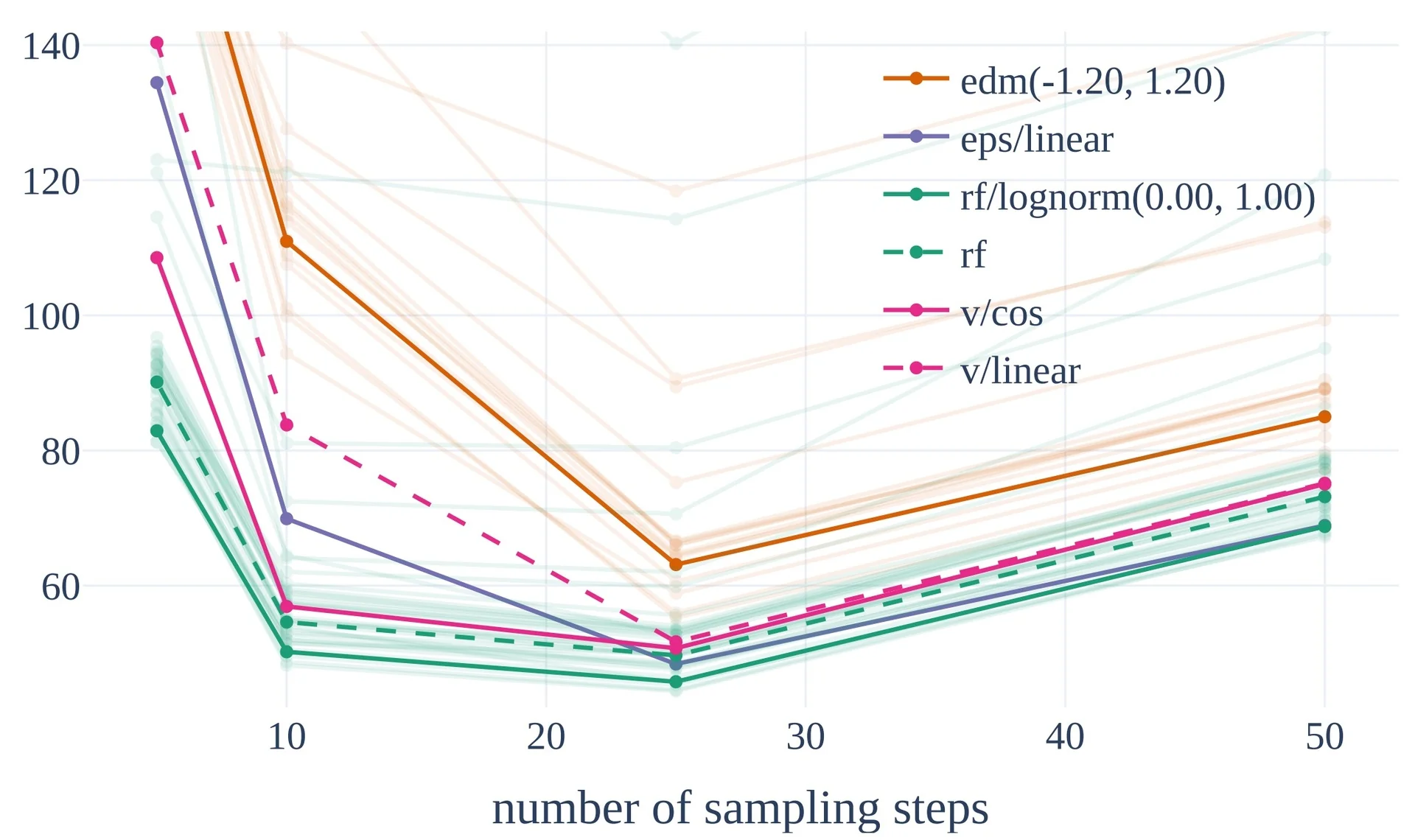
# SD3-style RF training: logit-normal timestep sampling for RF.
# z_t = (1-t) x0 + t eps, and the network predicts a velocity / equivalent target.

for step in range(num_steps):
    x0 = sample_data_latent()          # x0 ~ p0 (latent of an autoencoder)
    eps = sample_standard_normal()     # eps ~ N(0, I)

    u = normal(mean=m, std=s)          # e.g., m=0.0, s=1.0
    t = sigmoid(u)                     # logit-normal timestep

    zt = (1.0 - t) * x0 + t * eps
    v_target = eps - x0                # RF straight-line velocity

    v_pred = net(zt, t, cond_text)     # SD3 uses a multimodal transformer backbone
    loss = mse(v_pred, v_target)
    loss.backward()
    opt.step()
3. MM-DiT: Bidirectional Multimodal Diffusion Transformers Beyond optimizing the mathematical noise schedule, the SD3 authors identified the architectural backbone as a primary bottleneck for complex prompt understanding, spatial reasoning, and typography [150].
Historically, text-to-image models have forced text and image representations to interact using mathematically restrictive bottlenecks. Latent Diffusion Models (like SDXL) typically inject text via cross-attention into a U-Net [548].
This mechanism is inherently unidirectional: the image features are dynamically updated based on the text, but the text embeddings remain frozen, completely uncontextualized by the evolving spatial layout of the image. Conversely, early Diffusion Transformers (like the vanilla DiT) naïvely concatenate text and image tokens into a single sequence processed by shared transformer blocks [492].
This shared-weight approach creates a capacity coupling problem. Text tokens encode dense, discrete semantic concepts (e.g., grammatical syntax, object relations), whereas image patches encode sparse, continuous spatial frequencies (e.g., edges, textures, colors). Because MLPs function as non-linear feature dictionaries, forcing a single set of MLP weights to serve both of these fundamentally different data distributions wastes parameter capacity and dilutes modality-specific representations [150].
The Dual-Stream Solution. To bridge this modality gap, SD3 introduces the Multimodal Diffusion Transformer (MM-DiT).
Instead of forcing a compromised shared space, MM-DiT maintains entirely separate parameter sets for text and image streams throughout the network. Visual tokens and text tokens undergo their own independent LayerNorm and MLP operations. This allows each modality to undergo complex non-linear transformations strictly within its native dimensional space.
The two parallel streams only interact during the Self-Attention operation. Here, the sequences are temporarily concatenated, allowing the attention matrix to compute rich, bidirectional correlations. This is a profound shift from cross-attention: not only do the visual tokens attend to the text to understand what to draw, but the text tokens attend back to the visual features. This allows the text embeddings to dynamically update and contextualize themselves based on the current physical layout of the image—a mechanism that proved absolutely critical for complex spatial reasoning and accurate typography generation. After this joint attention step, the sequences are split back into their independent streams [150].
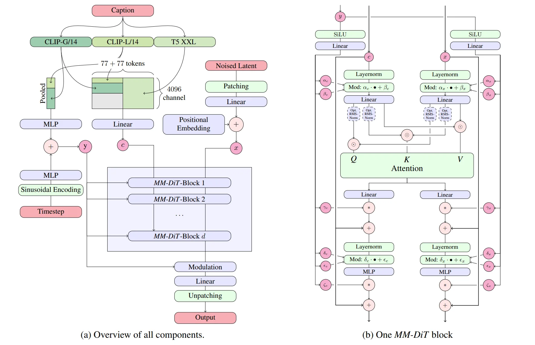
Convergence Advantage. This architectural decoupling is not merely a theoretical elegance; it yields massive empirical gains. In controlled scaling sweeps, the bidirectional routing and independent MLPs of MM-DiT systematically reduce validation loss and improve downstream sample quality (FID and CLIP scores) much faster than standard DiT, CrossDiT, and UViT-style baselines parameterized with equivalent compute. By preventing text and image features from competing for shared parameter capacity, the network learns the flow matching vector field significantly more efficiently [150].
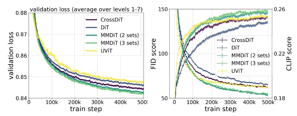
4. Stabilizing Large-Scale RF Transformers: QK-Normalization While the MM-DiT architecture theoretically enables bidirectional multimodal learning, scaling this continuous-time transformer to 8 billion parameters and high resolutions (e.g., \(1024 \times 1024\)) introduces severe numerical instabilities. Specifically, during mixed-precision training (bf16), the network is highly susceptible to an optimization failure known as attention entropy collapse [150].
The Mechanics of the Instability. In a standard transformer block, the self-attention matrix is computed by taking the dot product of Queries (\(Q\)) and Keys (\(K\)), scaled by the dimension size: \(\mbox{Softmax}(QK^T / \sqrt {d})\). As the network scales deeper and the spatial sequence lengths grow (due to higher resolution latent patches), the magnitudes of the unconstrained \(Q\) and \(K\) vectors tend to drift and grow uncontrollably, particularly in the final, deepest transformer layers.
When these bloated vectors are multiplied together, the resulting pre-softmax logits explode. The softmax function is notoriously sensitive to large magnitude inputs: a massive logit causes the softmax output to become exponentially “sharp,” effectively collapsing into a one-hot vector. This means a patch learns to attend to only one single other token, ignoring all other global context.
Mathematically, the entropy of the attention distribution plummets to near zero. When the attention matrix becomes a rigid set of 1s and 0s, the gradients either vanish entirely or trigger numerical overflows, resulting in catastrophic NaN losses that permanently halt training.
The Lightweight Fix: QK-Normalization. To prevent this, SD3 borrows a stabilization technique previously explored in discriminative Vision Transformers: QK-normalization. Before computing the dot product, the model explicitly normalizes both the Query and Key embeddings using Root Mean Square Normalization (RMSNorm) [781, 150].
By enforcing a strict, bounded magnitude on \(Q\) and \(K\), the dot product \(QK^T\) is geometrically constrained. The pre-softmax logits remain small and well-behaved, preserving a “soft” and distributed attention matrix (high entropy). SD3 applies this QK-normalization inside both the text and image streams of the MM-DiT blocks. This single mathematical constraint completely eliminates the instability, allowing massive 8B parameter models to train smoothly in bf16 without falling back to computationally slow full-precision (fp32) arithmetic.
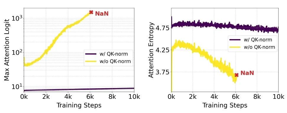
5. Resolution-Dependent Timestep Shifting: Scaling the Noise Schedule A subtle but critical failure mode in diffusion models occurs when scaling to higher resolutions. If a model is trained at a base resolution (e.g., \(256 \times 256\)) but sampled at a higher target resolution (e.g., \(1024 \times 1024\)) using the exact same continuous timestep schedule, the generative trajectory breaks down. The resulting images often suffer from severe overconfidence artifacts, disjointed structures, or oversaturation.
Why does this happen? The core insight of SD3 is that the exact same timestep \(t\) does not correspond to the same effective uncertainty across different resolutions [150].
The Statistical Intuition. To understand this, SD3 analyzes a “constant image” thought experiment. Imagine an image consisting of a single, uniform solid color. As the resolution increases, the total number of pixels \(n = H \cdot W\) increases.
During the forward noise process (Eq. (20.112)), independent Gaussian noise is added to each individual pixel. Because the neural network processes patches locally and globally via self-attention, it can effectively “average” the noise across these pixels to guess the underlying clean color. According to the Central Limit Theorem, the standard error of this average shrinks proportionally to \(1/\sqrt {n}\).
Therefore, a \(1024 \times 1024\) image with the exact same per-pixel noise variance as a \(256 \times 256\) image is statistically cleaner. The network has 16 times more spatial samples to cross-reference. SD3 formalizes this by defining an uncertainty proxy: \[ \sigma (t,n) \propto \frac {t}{1-t}\frac {1}{\sqrt {n}} \] This explicitly proves that at any fixed timestep \(t\), higher resolutions (larger \(n\)) are effectively less noisy. If we do not account for this, the model perceives the high-resolution image as being much closer to \(t=0\) than it actually is, causing it to prematurely stop generating large structural layouts and over-focus on high-frequency details.
The Shifting Formula. To maintain a consistent generative difficulty, we must deliberately inject more noise at higher resolutions. By mathematically equating the uncertainty at a lower base resolution \(n\) with the uncertainty at a higher target resolution \(m\) (i.e., \(\sigma (t_n, n) = \sigma (t_m, m)\)), SD3 derives an elegant, resolution-dependent timestep mapping:
\begin {equation} t_m = \frac {\sqrt {\frac {m}{n}}\,t_n}{1+\Big (\sqrt {\frac {m}{n}}-1\Big )t_n} \label {eq:chapter20_sd3_timestep_shift} \end {equation}
When moving to a higher-resolution generation, SD3 physically shifts the standard sampling schedule using this formula. This maps the original timestep \(t_n\) to a new, higher timestep \(t_m\), injecting the mathematically precise amount of extra noise required to prevent early structural collapse [150].
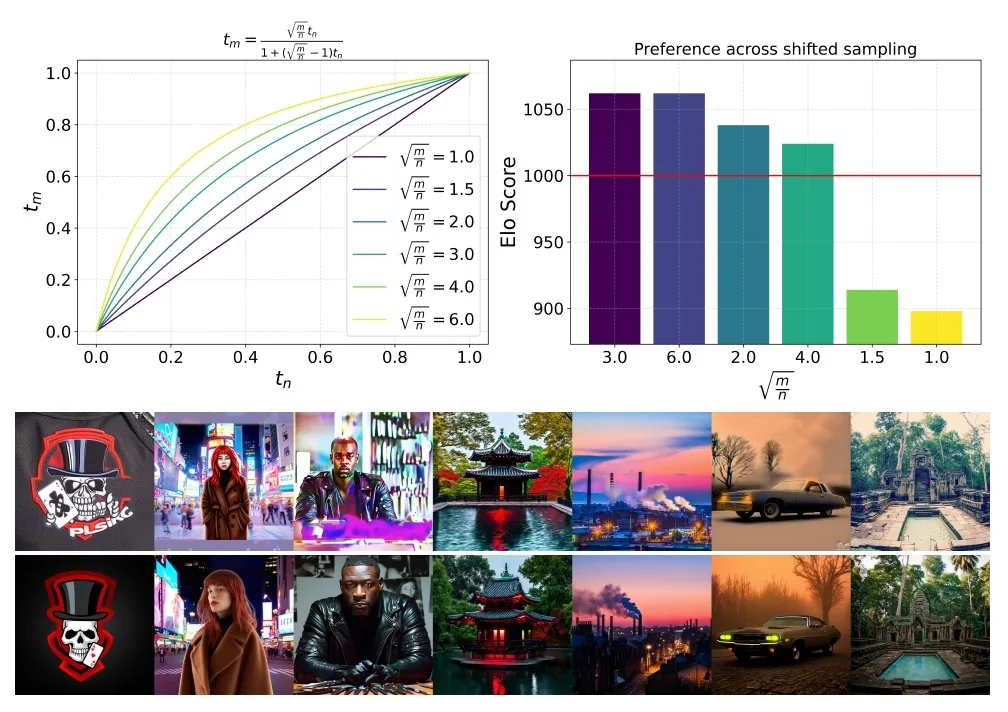
6. Scaling laws: validation loss as a proxy for generation quality A striking empirical finding is that SD3 training exhibits smooth scaling trends, and that validation loss strongly predicts holistic generation quality [150]. Across model sizes (parameterized by depth), lower validation loss correlates with (i) higher GenEval scores [177], (ii) improved human preference, and (iii) better T2I-CompBench performance [255].
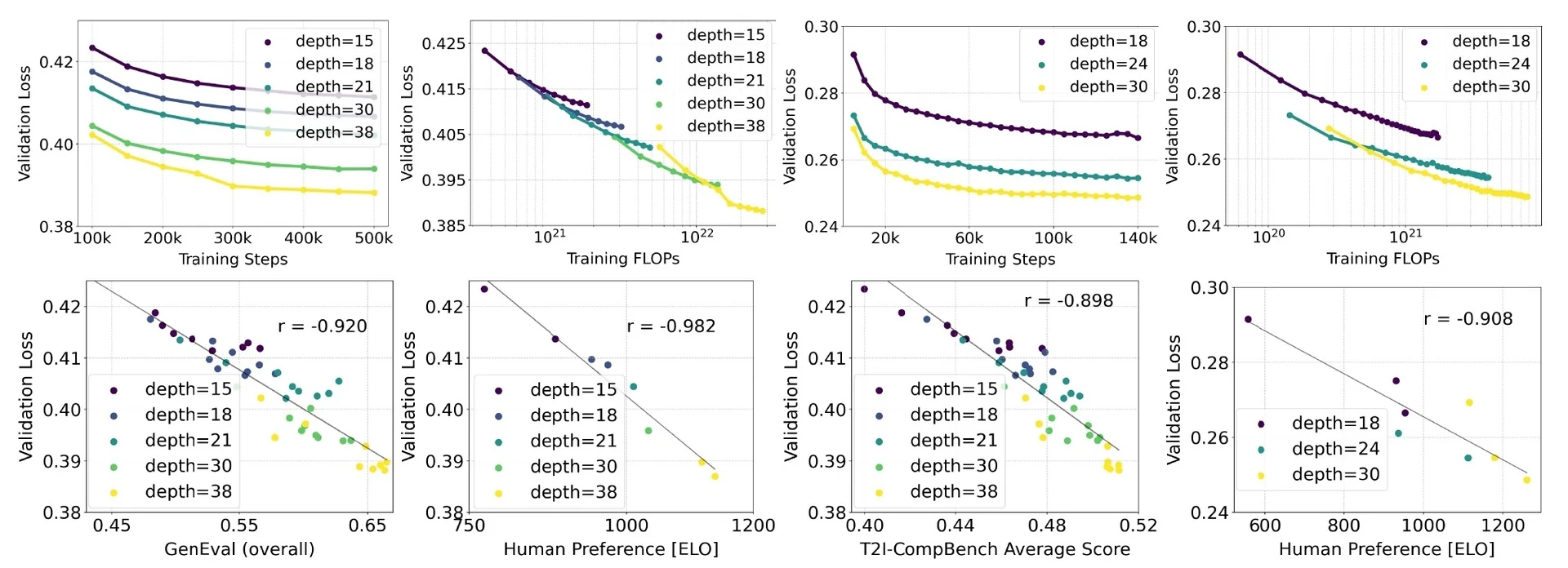
7. Text encoders, typography, and inference-time flexibility To improve text understanding, SD3 conditions on multiple frozen text encoders (CLIP L/14, OpenCLIP bigG/14, and T5-v1.1-XXL) [150, 517]. During training, each encoder is independently dropped out (reported dropout rate \(46.4\%\) per encoder), so at inference the model can use any subset [150]. This yields an explicit quality–memory trade-off: Table 7 in [150] reports that loading T5 requires \(\approx 19.05\) GB GPU memory, motivating optional removal for memory-constrained inference. Qualitatively, SD3 finds T5 particularly valuable for long spelled text and highly detailed prompts, while many everyday prompts remain competitive without it [150].
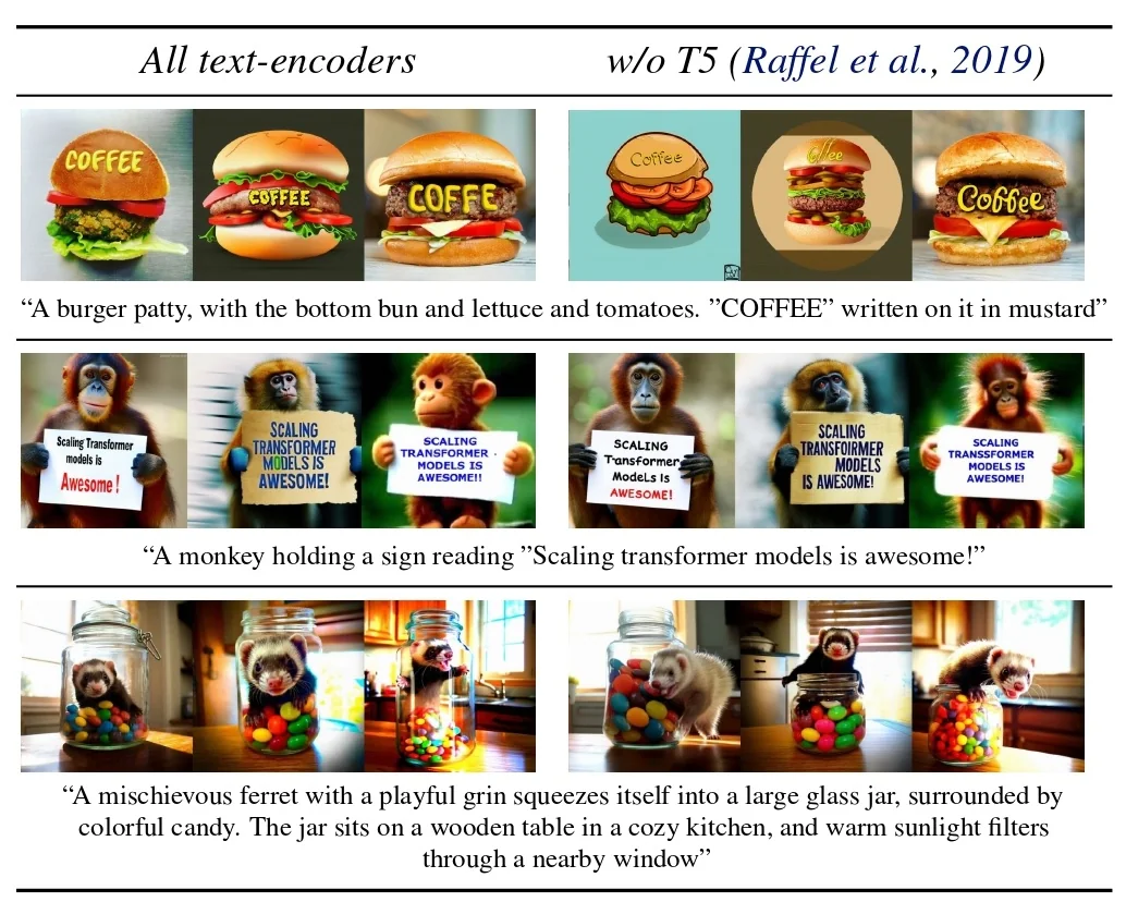
8. Improved Autoencoders: Increasing Latent Channel Depth Like all latent diffusion models, SD3 operates in the compressed latent space of a pretrained autoencoder [548]. A key but often overlooked design choice is the number of latent channels \(d\). Prior models such as SDXL used \(d=4\) channels, but the reconstruction quality of this autoencoder imposes an upper bound on achievable image fidelity. [150] find that increasing \(d\) significantly boosts reconstruction performance (measured by FID, perceptual similarity, and PSNR), with the gap between \(d=8\) and \(d=16\) becoming negligible for sufficiently deep generative models (depth \(\geq 22\)). SD3 therefore adopts a \(d=16\) channel autoencoder with a downsampling factor of \(f=8\), providing a richer latent representation at the cost of a proportionally larger latent tensor [150].
9. Human preference evaluation: aesthetics, prompt following, typography SD3 evaluates human preference on PartiPrompts [765], using separate rubrics for visual aesthetics, prompt following, and typography [150]. The results highlight a persistent pattern: typography is the hardest axis, and dropping T5 disproportionately hurts spelling relative to aesthetics.
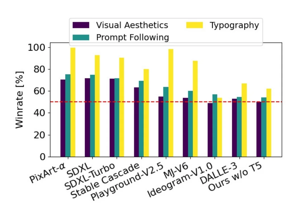
10. Optional Alignment: Preference Fine-Tuning via DPO Pretraining on massive datasets teaches a generative model the “physics” of image synthesis, but it does not inherently teach the model what humans find aesthetically pleasing or what constitutes perfect prompt adherence. To bridge this gap, SD3 demonstrates that continuous-time flow models are highly amenable to post-training alignment using Direct Preference Optimization (DPO) [516, 150].
Originally developed to align Large Language Models without the complexity of Reinforcement Learning with Human Feedback (RLHF), DPO operates directly on comparative data. For text-to-image models, the dataset consists of a text prompt and two generated images: one marked as “chosen” (preferred by humans) and one marked as “rejected”.
The DPO loss function modifies the model’s weights to increase the likelihood of the probability trajectory leading to the chosen image, while penalizing the trajectory of the rejected image. Following Wallace et al. [673], the SD3 authors apply DPO through Low-Rank Adaptation (LoRA) with rank 128 on all linear layers, fine-tuning for 4k iterations on the 2B model and 2k iterations on the 8B model. Human preference evaluations confirm that DPO-finetuned models are consistently preferred over their base counterparts in both prompt following and overall visual quality [150].
Summary and Bridge to Distillation Stable Diffusion 3 establishes the definitive modern blueprint for scaling continuous-time generative models. It proves that the optimal paradigm is to first straighten the generative trajectory (Rectified Flow), and then allocate the engineering budget toward solving the practical bottlenecks:
- Where to train along the path (Logit-Normal timestep sampling).
- How to process conflicting modalities (MM-DiT’s dual streams).
- How to stabilize massive parameter counts at high resolutions (QK-normalization and resolution-dependent timestep shifting).
However, while SD3 minimizes ODE solver error and achieves state-of-the-art fidelity, it still fundamentally relies on sequential, multi-step numerical integration (typically 20 to 28 steps) during inference.
This raises a tantalizing theoretical question: If Rectified Flow perfectly straightens the probability path from noise to data, why can we not traverse that straight line in exactly one single step?
This exact premise motivates our next major milestone: InstaFlow. We will explore how researchers leverage distillation to force these straight-line models to jump from pure noise to a pristine image instantly. From there, we will navigate the broader landscape of accelerated continuous generation—exploring Latent Consistency Models (LCM) and Distribution Matching Distillation (DMD)—before ultimately breaking free from continuous-time ODE solvers entirely through the discrete-time revolutions of Discrete Flow Matching (DFM), Generator Matching (GM), and Transition Matching (TM).
Enrichment 20.11.15: InstaFlow: 1-Step Generation via Reflow and Distillation
Why one-step distillation is hard: the linearization error A one-step generator is an extreme discretization: it tries to jump from \(x_0\sim \pi _0\) to \(x_1\sim \pi _1\) with effectively \(N=1\). If the teacher’s probability-flow ODE has curved trajectories, then the straight chord from \(x_0\) to \(x_1\) is a poor proxy for the integral curve. In that regime, a student must learn a highly non-linear “shortcut” map \(x_0\mapsto x_1\), which empirically leads to unstable training and degraded details.
InstaFlow: straighten first, then distill InstaFlow [390] applies Rectified Flow’s coupling-repair mechanism at text-to-image scale. The pipeline is:
- 1.
- Text-conditioned Reflow (teacher conditioning): starting from a pre-trained diffusion T2I model, perform reflow under conditioning (prompts / CFG) to obtain a 2-Rectified Flow teacher. This step straightens trajectories and refines the noise–image coupling [390].
- 2.
- One-step Distillation: distill from the 2-Rectified teacher into a single-step student. Because the teacher’s paths are now much closer to straight, the one-step jump has far smaller linearization error, and the student can preserve high-frequency structure.
A central empirical finding in [390] is that direct distillation fails, while distillation after reflow succeeds: 2-Rectified Flow is a substantially better teacher (smaller quality gap; closer visual match under the same \(x_0\) and prompt), precisely because reflow improves the coupling and straightens the geometry before the student is asked to “jump” in one step.
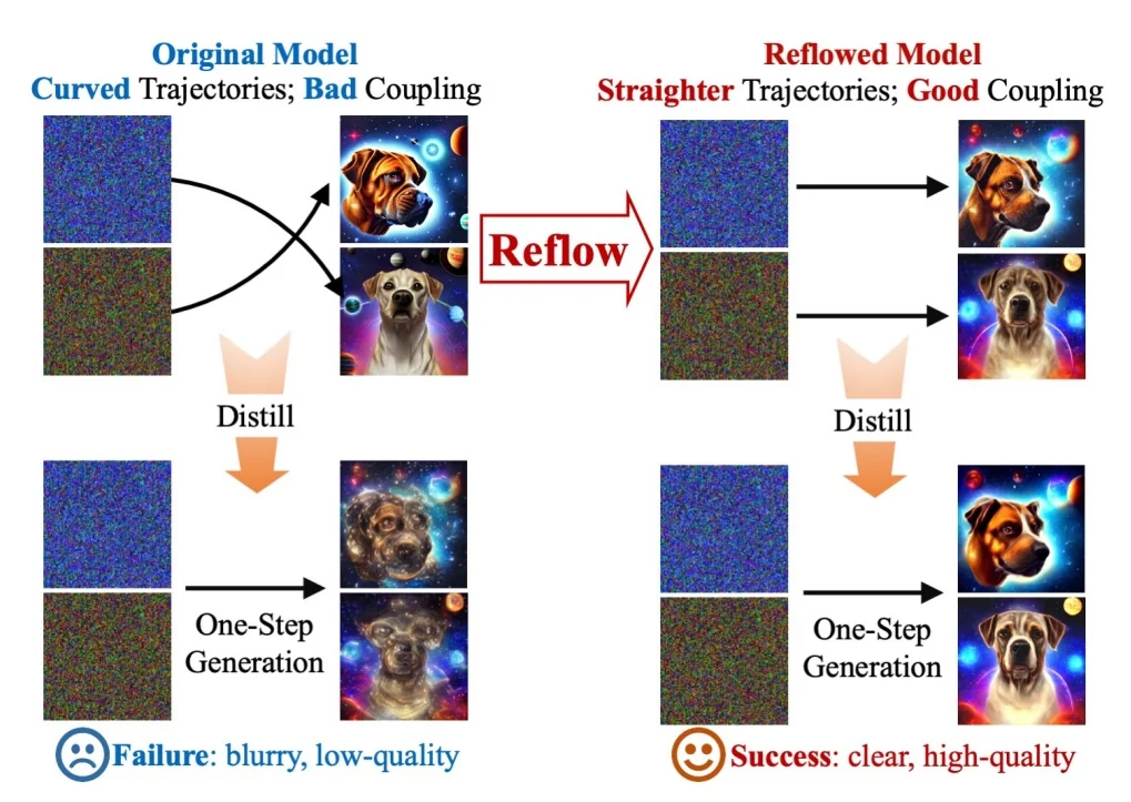
Rectified Flow (2022) vs. InstaFlow (2024): Same Mechanism, Different Goals Although both works rely on the reflow mechanism, they address different stages of the generative pipeline:
- Rectified Flow (The Theory): [389] introduces Reflow as a recursive operator to minimize transport cost. It focuses on the theoretical limit (\(k \to \infty \)) where the coupling becomes deterministic (Monge map) and trajectories become perfectly straight, enabling ODE solvers to work with fewer steps.
- InstaFlow (The Scaling): [390] applies this to large-scale Text-to-Image models with a specific finding: Reflow is a prerequisite for Distillation. Directly distilling a standard diffusion model (curved) into one step fails because the student cannot approximate the curve. InstaFlow shows that a single round of Reflow (creating a 2-Rectified Flow) is the ”sweet spot”: it straightens the flow enough to make one-step distillation viable, without the computational cost of infinite recursion.
Implementation Note: Why Practitioners Prefer Rectified Objectives Beyond the geometry, the Rectified Flow formulation (\(\dot {Z}_t = v\)) has become the default for modern models (like Stable Diffusion 3 and Flux) due to Numerical Stability.
- Diffusion Singularities: Standard variance-preserving diffusion schedules often require ”hacks” (like offset noise or \(\epsilon \)-clipping) near \(t=0\) and \(t=1\) because the signal-to-noise ratio approaches singularities (infinity or zero).
- Clean Velocity: The rectified target is simply the velocity \(v = X_1 - X_0\). Since both data \(X_1\) and noise \(X_0\) are bounded (e.g., in \([-1, 1]\)), the target \(v\) is always finite and well-behaved for all \(t \in [0, 1]\). This allows for clean training without ”epsilon” cutoffs.
Takeaway Rectified Flow transforms ”straightness” from a local property (of training pairs) into a global property (of the vector field). InstaFlow demonstrates that this global straightness is the hidden key to one-step generation. By treating Reflow as a ”geometry conditioner”, we repair the teacher’s trajectories before distillation, reducing the linearization error and allowing the student to successfully learn a one-step shortcut.
Enrichment 20.11.16: SiT: The Unifying ”Interpolant” Framework
Beyond Diffusion vs. Flow Matching: The ”Interpolant” Abstraction What changed? Previously, models were often ”bundled”.
- If you used DiT [492], you implicitly bought into a specific ”package”: a Transformer backbone plus a curved diffusion path plus noise prediction (\(\epsilon \)).
- If you used Rectified Flow, you bought a different package: a straight path plus velocity prediction (\(v\)).
The SiT Innovation: Unbundling. SiT (Scalable Interpolant Transformers) [419] breaks these bundles apart. It treats the neural architecture (the Transformer) and the movement dynamics (the Path) as separate, mix-and-match components.
How it works: The ”Interpolant” Mixer. Instead of hard-coding a single diffusion schedule, SiT defines a flexible family of interpolants: \[ x_t = \alpha (t) x_0 + \beta (t) x_1. \] By changing \(\alpha (t)\) and \(\beta (t)\) (and, optionally, the sampling noise level), this abstraction spans a broad family of diffusion- and flow-style transports as special cases—including standard variance-preserving (VP) diffusion-style mixing and the linear (Rectified-Flow-style) path.
The Result. This lets SiT search for a ”Goldilocks” configuration: keep the DiT architecture (excellent scaling behavior) but swap the dynamics to Linear Interpolants (straight, Rectified-Flow-style geometry), which yields significantly better results than the original DiT training choices.
Step-by-Step Derivation: From ”Path Design” to ”Velocity Target” How do we translate a high-level choice about geometry (the path) into a concrete loss function for a neural network? SiT breaks this down into four logical steps.
- 1.
- Step 1: Design the Path (The Interpolant). We start by defining where a particle should be at time \(t\), given a specific start (noise \(x_0\)) and end (data \(x_1\)). \[ x_t = \alpha (t) x_0 + \beta (t) x_1. \] Intuition: This is a ”mixing recipe”. \(\alpha (t)\) controls how much noise remains; \(\beta (t)\) controls how much data is revealed.
- 2.
- Step 2: Derive the Velocity (The Physics). To simulate this path with an ODE, we need to know the velocity (tangent vector). We find this by taking the time derivative of the position: \[ u_t(x_0, x_1) \;=\; \frac {d}{dt}x_t \;=\; \dot {\alpha }(t) x_0 + \dot {\beta }(t) x_1. \] Example (Rectified Flow): If we choose the linear path \(\alpha (t) = 1-t\) and \(\beta (t) = t\), then \(\dot {\alpha } = -1\) and \(\dot {\beta } = 1\). The velocity becomes simply: \[ u_t = x_1 - x_0. \] This recovers the intuitive ”vector pointing straight at the data” we used in Rectified Flow.
- 3.
- Step 3: Learn the Vector Field (The Network). Crucially, during
inference, the model sees \(x_t\) but does not know \(x_0\) or \(x_1\). It cannot calculate
the exact velocity \(u_t\). Therefore, we train a network \(v_\theta (x_t, t)\) to predict the
conditional expectation of this velocity.
The loss function forces the network to match the physical velocity derived in Step 2: \[ \mathcal {L}_{\mbox{SiT}} = \mathbb {E}_{x_0, x_1, t} \left [ \underbrace {|| v_\theta (x_t, t) - (\dot {\alpha }(t) x_0 + \dot {\beta }(t) x_1) ||^2}_{\mbox{Network Output} \approx \mbox{Physical Velocity}} \right ]. \]
- 4.
- Step 4: The Stochastic Extension (The SDE Knob). Finally, SiT
generalizes this by allowing a diffusion coefficient \(w(t)\) to be added during
sampling.
- If \(w(t)=0\): We get a deterministic ODE (Flow Matching).
- If \(w(t)>0\): We inject noise at every step, turning the process into a stochastic SDE.
SiT vs. DiT: Same Body, Different Brain The original DiT paper [492] demonstrated that Transformers scale well for diffusion, but it locked the training dynamics into a standard, pre-defined ”package” (VP schedule, \(\epsilon \)-prediction).
SiT [419] keeps the exact same DiT Transformer backbone (the ”Body”) but treats the training dynamics (the ”Brain”) as a set of tunable knobs. By optimizing these knobs, SiT achieves better performance with the same compute.
-
Knob 1: The Path Geometry \((\alpha , \beta )\).
- DiT (Standard): Uses a variance-preserving (VP) mixing rule (often written as \(\alpha _t^2 + \beta _t^2 = 1\)), i.e., the coefficients trace a curved schedule in coefficient space (cosine/sine-style mixing) rather than the straight chord \(\alpha _t=1-t,\ \beta _t=t\). Relative to the linear interpolant, this typically induces more curvature in the induced transport geometry, which increases sensitivity to coarse discretization.
- SiT (Optimized): Advocates for a Linear Interpolant (e.g., \(\alpha (t)=1-t,\ \beta (t)=t\)), which yields straight chords (as in Rectified Flow) and is empirically easier to learn and discretize.
-
Knob 2: The Prediction Target.
- DiT (Standard): Predicts noise \(\epsilon \). Depending on the schedule and parameterization, \(\epsilon \)-targets can become poorly conditioned at the extremes of the trajectory (very high or very low SNR), which can make optimization more delicate.
- SiT (Optimized): Predicts velocity \(v\). For linear interpolants (Rectified-Flow-style), the target reduces to \(x_1-x_0\) (time-independent), and more generally velocity targets tend to vary smoothly with \(t\), which often yields better-scaled regression throughout the path.
-
Knob 3: ODE vs. SDE Sampling (Determinism vs. Stochasticity).
- ODE Sampling (\(w(t)=0\)). This yields a deterministic probability flow. Deterministic trajectories are often preferred for speed and for workflows that benefit from repeatability (and, in continuous time, reversibility of the flow up to numerical error).
- SDE Sampling (\(w(t)>0\)). SiT introduces a continuous noise scale during inference, which can be written schematically as \[ dX_t = v_\theta (X_t,t)\,dt + w(t)\,dW_t. \] Empirically, adding controlled noise during sampling can improve perceptual quality / FID in some regimes by reducing sensitivity to discretization and modeling error, and SiT treats this inference-time diffusion strength as a tunable knob.
The Training Scheme: One Loop to Rule Them All How do we train a model when the ”Physics” (Interpolant) and the ”Target” (Prediction) are tunable knobs? The training loop remains identical; only the Label Definition changes.
The Algorithm (Single Step):
- 1.
- Sample Data & Noise: Draw a clean image \(x_1 \sim \mbox{Data}\) and a Gaussian noise sample \(x_0 \sim \mathcal {N}(0, I)\).
- 2.
- Sample Time: Draw a time \(t \in [0, 1]\).
- 3.
- Construct the Input (The Path): Mix them using the chosen schedule functions \(\alpha (t)\) and \(\beta (t)\): \[ x_t = \alpha (t)x_0 + \beta (t)x_1. \]
- 4.
- Compute the Target (Knob 2): Here is where the ”multi-task”
flexibility comes in. Depending on what we want the network to
predict, we calculate a different target label \(Y_{\mbox{target}}\) from the same \(x_0, x_1\):
- Option A: Velocity Prediction (\(v\)): Target is the time derivative (Flow Matching default). \[ Y = \dot {\alpha }(t)x_0 + \dot {\beta }(t)x_1. \]
- Option B: Noise Prediction (\(\epsilon \)): Target is the starting noise (Diffusion default). \[ Y = x_0. \]
- Option C: Data Prediction (\(x\)): Target is the final image. \[ Y = x_1. \]
- 5.
- Optimize: Feed \(x_t\) into the network \(F_\theta (x_t, t)\) and minimize the error against the chosen target: \[ \mathcal {L} = || F_\theta (x_t, t) - Y_{\mbox{target}} ||^2. \]
How ”Velocity” Solves ”Diffusion” You might ask: If we train to predict velocity (\(v\)), how does that help us remove noise (\(\epsilon \))?
Because the relationships are linear, predicting one variable unlocks all of them. For the standard Rectified Flow interpolant (\(\alpha =1-t, \beta =t\)): \[ x_t = (1-t)x_0 + t x_1 \quad \mbox{and} \quad v_t = x_1 - x_0. \] If the network predicts \(v_t\), we can analytically recover the denoised image \(x_1\) using simple algebra: \[ x_1 = x_t + (1-t) \cdot \underbrace {v_\theta (x_t)}_{\mbox{predicted}}. \]
The Takeaway: SiT shows that while you can choose any target,Velocity is the best choice because it mixes \(x_0\) and \(x_1\) in a way that remains stable (finite variance) throughout the entire process, whereas \(\epsilon \) targets explode near \(t=0\).
Scaling Evidence: Larger SiT Improves Sample Quality A practical takeaway from SiT is that once the dynamics are expressed in this interpolant form, Transformer scaling behaves cleanly: larger backbones produce visibly higher-quality samples under identical sampling conditions.
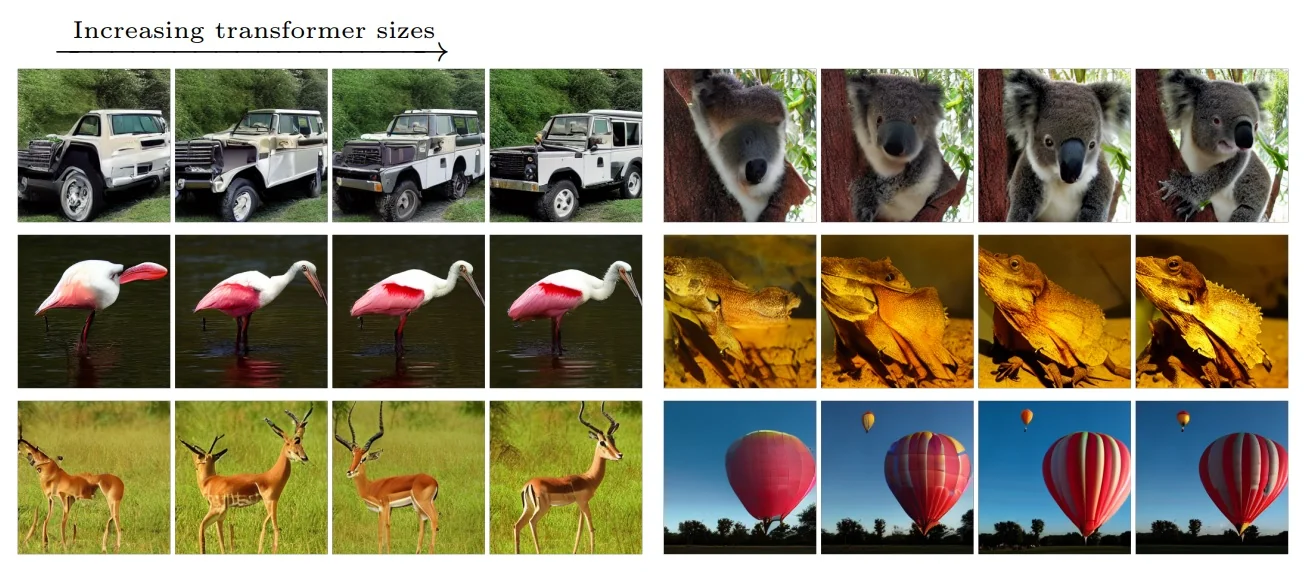
Connection to Rectified Flow and InstaFlow: Geometry First, Distillation Second SiT’s message is complementary to Rectified Flow and InstaFlow; it provides the theoretical map that places them in context.
- Rectified Flow (The Insight): [389] Identifies trajectory geometry (straightness) as a key bottleneck for fast sampling. Its rectification procedure induces a new deterministic coupling with provably non-increasing convex transport costs, and recursive rectification yields increasingly straight trajectories that can be simulated accurately with coarse discretization (even a single Euler step in favorable regimes).
- InstaFlow (The Application): [390] Exploits this at scale. It shows that straight geometry is a prerequisite for distillation: you must straighten the teacher (Reflow) before you can successfully distill it into a one-step student.
- SiT (The Map): [419] Provides the unifying lens. It shows that standard Diffusion is simply a ”Curved Interpolant” and Rectified Flow is a ”Linear Interpolant”. By sweeping over this design space, SiT confirms empirically that Linear (Straight) is indeed the optimal default, turning the intuition of Rectified Flow into a rigorous design principle.
Takeaway SiT reframes ”Diffusion vs. Flow Matching” from a debate about algorithms into a choice of settings on the same Interpolant Machine: choose \((\alpha ,\beta )\) to set the path geometry, choose the target (velocity vs. noise), and choose \(w_t\) to interpolate between ODE and SDE sampling.
Crucially, SiT proves that Geometry matters more than Architecture. Even with the exact same Transformer backbone (DiT), simply switching from a curved path to a straight path yields significant performance gains, confirming that straight geometry is the easiest geometry to learn.
Enrichment 20.11.17: Consistency Models: Teleporting to the Origin
From “Straightening the Path” (Rectified Flow) to “Learning the Map” (Consistency) Recent flow-based methods, most notably Rectified Flow (and its one-step derivative InstaFlow), reframe generation as a geometry problem: they aim to straighten probability paths so the underlying ODE is close to a constant-velocity trajectory, making numerical integration dramatically easier [389, 390]. However, even an approximately straight path still incurs an integration tax: producing high-quality samples typically requires multiple function evaluations (NFE), because any residual curvature turns a single large solver step into discretization drift.
The limitation: residual curvature still costs NFE. Rectified Flow reduces path curvature by learning a more transport-aligned velocity field, but a single large solver step can still incur discretization error whenever the learned trajectories remain even mildly curved. The reflow procedure proposed in Rectified Flow can be viewed as an optional acceleration mechanism that further improves straightness by iteratively regenerating and re-fitting trajectory pairs; it is a practical way to push toward reliably low-step sampling, but it is not the only route to few-step performance.
The consistency solution (CM). Consistency Models (CM) [603] bypass the need to straighten the path entirely. Instead of forcing the vector field to be linear, CMs accept that the underlying trajectory may be curved and learn the solution map explicitly: a direct mapping \(f_\theta (x_\sigma ,\sigma )\to x_\epsilon \) that jumps from (almost) anywhere on the path to the trajectory endpoint. This allows distilling standard diffusion teachers into one-step (or few-step) samplers without costly generate-then-retrain loops.
Notation: inheriting the EDM framework Consistency Models are built directly on top of the EDM formulation. We continue to use the noise standard deviation \(\sigma \) as the independent variable:
- The process runs from \(\sigma _{\max }\) (pure noise) down to \(\sigma _{\min }\) (near-clean data).
- Notation switch: following the CM literature, we denote the minimum noise level by \(\epsilon \equiv \sigma _{\min }\).
- For occasional alignment with CM notation, we will also use \(T \equiv \sigma _{\max }\).
As in EDM, noisy inputs are formed by additive perturbations: \begin {equation} \label {eq:chapter20_cm_forward_perturbation} x_\sigma = x_0 + \sigma \,\xi , \qquad \xi \sim \mathcal {N}(0,\mathbf {I}), \qquad \sigma \in [\epsilon ,\sigma _{\max }]. \end {equation}
The singularity problem: why stop at \(\epsilon \)? Ideally, we would map directly to perfectly clean data at \(\sigma =0\). However, the EDM probability flow ODE contains a velocity term scaled by \(1/\sigma \) (see Eq. 20.75), which becomes numerically ill-conditioned as \(\sigma \to 0\). For this reason, Consistency Models define their target as the state at the safety buffer \(\epsilon \), rather than at exactly \(0\).
The “numerical origin” (\(x_\epsilon \)). Because \(\epsilon \) is chosen to be microscopic (e.g., \(\epsilon \approx 0.002\) in common EDM/CM schedules), \(x_\epsilon \) is visually indistinguishable from \(x_0\), allowing us to treat it as the “clean” endpoint while keeping the math stable.
The core object: the endpoint map Consider the Probability Flow (PF) ODE associated with a diffusion model. Since the ODE is deterministic, it defines a unique transport map \(\Phi _{\sigma \rightarrow \sigma '}(\cdot )\) that moves states along trajectories. Consistency Models learn the endpoint map back to \(\epsilon \): \begin {equation} \label {eq:chapter20_cm_endpoint_map} f_\theta (x,\sigma )\;\approx \;\Phi _{\sigma \rightarrow \epsilon }(x). \end {equation} Intuitively: given a noisy point \(x_\sigma \), predict the trajectory’s near-clean endpoint immediately.
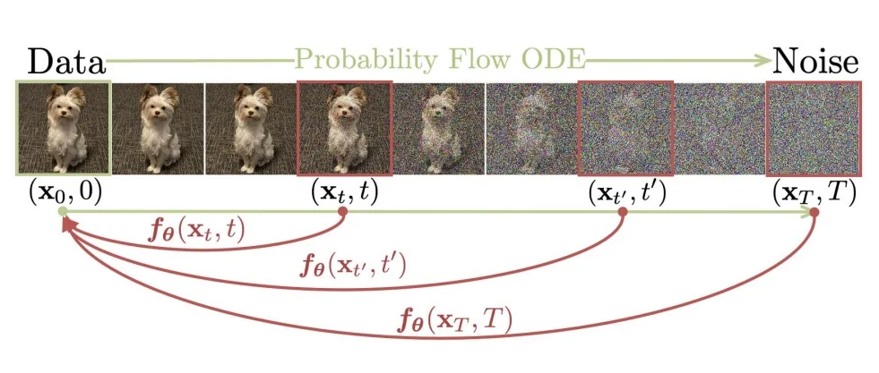
The consistency property (self-agreement) The defining innovation is replacing the requirement to simulate trajectories with the requirement to recognize them. Formally, if \(x_{\sigma '}=\Phi _{\sigma \rightarrow \sigma '}(x_\sigma )\) lies on the same trajectory (with \(\sigma >\sigma '\)), the decoded endpoint must be invariant: \begin {equation} \label {eq:chapter20_cm_consistency_condition} f_\theta (x_\sigma ,\sigma ) \;=\; f_\theta (x_{\sigma '},\sigma ') \;\approx \; x_\epsilon . \end {equation}
Why is this objective unique?
- Diffusion/SiT (The Compass): learns a tangent (velocity). It says “North is that way”. You must integrate repeatedly (large NFE) to avoid drift.
- Consistency (The Signpost): learns the endpoint. It says “The destination is at \((X,Y)\)”. It enables solver-free teleportation (NFE \(=1\)).
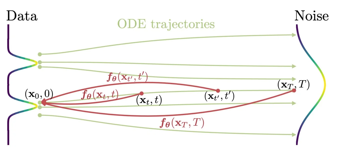
Clarification: why not just predict \(\hat {x}_0\) in one step? A common confusion is why we need a new model class when standard diffusion networks (predicting \(\epsilon \), \(v\), or \(\hat {x}_0\)) can already compute a one-shot estimator \(\hat {x}_0(x_\sigma )\). The key difference is what the network is trained to represent in the one-step regime:
- One-shot regression tends to a conditional mean. If we train \(\hat {x}_0(x_\sigma )\) with an \(\ell _2\) objective on pairs sampled from Eq. 20.117, the Bayes-optimal predictor is \(\mathbb {E}[x_0\mid x_\sigma ]\). At large \(\sigma \), this conditional can be highly multimodal, so the mean behaves like a blurry superposition. Iterative samplers resolve this ambiguity by repeatedly reconditioning.
- CMs target a trajectory-specific endpoint map. In contrast, the PF-ODE defines a deterministic mapping from each point on the trajectory to its endpoint. The consistency loss enforces agreement of \(f_\theta (\cdot ,\cdot )\) across adjacent points on the same teacher trajectory, forcing the model to approximate \(\Phi _{\sigma \to \epsilon }\) rather than a generic conditional mean [603]. To further guarantee sharpness, the distance metric \(d(\cdot ,\cdot )\) used during training is typically a perceptual loss (LPIPS) rather than a simple pixel-wise \(\ell _2\) error. Empirically, Song et al. find that using LPIPS as the metric \(d(\cdot ,\cdot )\) yields substantially better distillation performance than \(\ell _1\) or \(\ell _2\) when the model output is an image [603, 800]. Intuitively, perceptual metrics better align the training signal with semantic structure and tend to discourage overly smoothed “average-looking” predictions in the few-step regime.
Why trivial collapse is prevented: the boundary-preserving “zipper” A naive invariance loss admits a degenerate solution: if the network learns to output a constant value for all inputs (e.g., \(f_\theta (x,\sigma ) = \mathbf {0}\)), the self-consistency error \(\|f_\theta (x_\sigma ,\sigma )-f_\theta (x_{\sigma '},\sigma ')\|^2\) trivially drops to zero. CMs prevent this by hard-wiring the boundary condition at \(\sigma =\epsilon \) via a skip-connection parameterization [603]: \begin {equation} \label {eq:chapter20_cm_skip_parameterization} f_\theta (x_\sigma ,\sigma ) = \underbrace {c_{\mathrm {skip}}(\sigma )\,x_\sigma }_{\mbox{Pass-through}} + \underbrace {c_{\mathrm {out}}(\sigma )\,F_\theta (x_\sigma ,\sigma )}_{\mbox{Neural Correction}}. \end {equation} Here, \(F_\theta \) is the raw neural network (the U-Net/Transformer), and \(f_\theta \) is the full Consistency Model. Crucially, the loss function is computed on the final combined output \(f_\theta (x_\sigma , \sigma )\), not on the raw neural network. \(F_\theta \) simply acts as a learned correction engine inside this architectural wrapper.
Defining the gates. To enforce the boundary condition \(f_\theta (x_\epsilon , \epsilon ) = x_\epsilon \), the scaling coefficients (gates) must satisfy \(c_{\mathrm {skip}}(\epsilon )=1\) and \(c_{\mathrm {out}}(\epsilon )=0\). Following the variance-scaling principles of EDM, Consistency Models define these gates as \(\epsilon \)-shifted analytic functions:
\begin {equation} \label {eq:chapter20_cm_gates} c_{\mathrm {skip}}(\sigma ) = \frac {\sigma _{\mbox{data}}^2}{(\sigma -\epsilon )^2 + \sigma _{\mbox{data}}^2}, \qquad c_{\mathrm {out}}(\sigma ) = \frac {\sigma _{\mbox{data}}(\sigma -\epsilon )}{\sqrt {\sigma _{\mbox{data}}^2 + \sigma ^2}}. \end {equation}
Where \(\sigma _{\mbox{data}}\) is the standard deviation of the clean dataset (typically \(0.5\)).
The logic of the chosen gates: These functions are not arbitrary; they dictate how much the model “trusts” the noisy input versus its own hallucination at different noise levels:
- 1.
- At the boundary (\(\sigma = \epsilon \)): The terms evaluate exactly to \(c_{\mathrm {skip}} = 1\) and \(c_{\mathrm {out}} = 0\). The neural network is completely multiplied by zero. The model is mechanically forced to act as the identity map, passing \(x_\epsilon \) straight through.
- 2.
- At high noise (\(\sigma \gg \epsilon \)): The pass-through gate \(c_{\mathrm {skip}}\) rapidly decays to \(0\), meaning the model ignores the input (which is mostly useless static). Meanwhile, \(c_{\mathrm {out}}\) approaches \(\sigma _{\mbox{data}}\). Since \(F_\theta \) is initialized to output unit-variance predictions, multiplying it by \(\sigma _{\mbox{data}}\) re-scales the network’s output to match the physical magnitude of real images.
Intuition (“The zipper”). Let \(\epsilon =\sigma _0<\sigma _1<\cdots <\sigma _N=\sigma _{\max }\). Training enforces consistency between neighboring noise levels \((\sigma _{n+1},\sigma _n)\). Because \(\sigma _0\) is mathematically anchored to the true data via the parameterization, matching \(\sigma _1\) to \(\sigma _0\) forces the network’s prediction at \(\sigma _1\) to become correct. Once \(\sigma _1\) is correct, the loss matching \(\sigma _2\) to \(\sigma _1\) forces \(\sigma _2\) to become correct, and so on. The “truth” physically zips upward from the clean boundary all the way to pure noise.
The Distillation Setup: What are the constraints? To train a consistency model, we need a source of truth about the trajectories. A natural question is: what are the constraints on the teacher and student models?
- Teacher constraints (Any PF-ODE): Consistency learning is framework-agnostic. What does it actually mean in practice to “define a deterministic PF-ODE”? It simply means the teacher must be a pre-trained neural network capable of telling us which direction to move to remove noise. Crucially, it does not matter how the teacher was trained. Whether the teacher learned to predict noise (\(\epsilon \)-prediction, like DDPM/EDM), to predict the clean image (\(x_0\)-prediction), or to predict velocity (\(v\)-prediction, like Rectified Flow or SiT), all of these are mathematically equivalent under the hood. They can all be algebraically converted into a local tangent vector. In practice: We plug the frozen teacher into a standard ODE solver (like Euler or Heun). We feed it a noisy image, it outputs a direction, and the solver takes a tiny step along that vector to produce a slightly cleaner image. This solver-guided step generates the “ground truth” path that the student will learn to skip.
- Architecture constraints (The Wrapper): The student’s internal neural backbone (\(F_\theta \)) can be any architecture—a Convolutional U-Net or a Transformer (DiT/SiT). It is typically initialized with the teacher’s weights. The only strict architectural constraint is that the student must be wrapped in the boundary-preserving “zipper” parameterization (Eq. 20.120) to prevent the loss from collapsing to zero.
A step-by-step derivation: The Distillation “Triangle” We enforce consistency on a discrete noise grid \(\sigma _0=\epsilon <\sigma _1<\cdots <\sigma _N=\sigma _{\max }\). In the standard Consistency Distillation (CD) framework, a single training step operates by forming a logical “triangle” connecting three points: the current noisy state, a slightly less noisy state, and the clean origin.
- 1.
- Sample the start point: Draw real data \(x_0 \sim p_{\mbox{data}}\) and random noise \(\xi \sim \mathcal {N}(0,\mathbf {I})\) to form a noisy point \(x_{\sigma _{n+1}} = x_0 + \sigma _{n+1}\xi \).
- 2.
- The Teacher’s Local Step (The Ground Truth Path): We use the frozen pretrained teacher to simulate a single, highly accurate ODE solver step (typically a 2nd-order Heun step) from \(\sigma _{n+1}\) down to the adjacent level \(\sigma _n\). This yields the point \(\hat {x}_{\sigma _n}\). Because this step is tiny, discretization error is minimal; we trust this as the “true” trajectory.
- 3.
- The Target’s Prediction (The Anchor): We feed this slightly cleaner point \(\hat {x}_{\sigma _n}\) into an Exponential Moving Average (EMA) copy of the student network, denoted \(f_{\theta ^-}\). This target network predicts the clean origin.
- 4.
- The Student’s Jump (The Learner): We feed the original, noisier point \(x_{\sigma _{n+1}}\) into the active student network \(f_\theta \). The student attempts to predict the clean origin in a single jump.
The consistency loss penalizes the difference between the Student’s prediction and the Target’s prediction: \begin {equation} \label {eq:chapter20_cm_consistency_loss} \mathcal {L}_{\mbox{cons}} = \mathbb {E}_{n,\,x_{\sigma _{n+1}}} \Big [ d\!\Big ( \underbrace {f_\theta (x_{\sigma _{n+1}},\sigma _{n+1})}_{\mbox{Student's Jump}}, \; \underbrace {\operatorname {stopgrad}\big (f_{\theta ^-}(\hat {x}_{\sigma _n},\sigma _n)\big )}_{\mbox{EMA Target from Teacher's Step}} \Big ) \Big ], \qquad \hat {x}_{\sigma _n}\approx \Phi _{\sigma _{n+1}\to \sigma _n}(x_{\sigma _{n+1}}). \end {equation} Intuition: The student asks, “If I jump straight to the end from here, do I land in the same place as the target network would if it started one step further down the true path?”. By using an EMA network (\(f_{\theta ^-}\)) rather than the active weights, the target remains stable, preventing the training from spiraling into a degenerate feedback loop.
Training schemes: Distill, Train-from-Scratch, or Tune Depending on compute budgets and available pretrained models, the consistency objective is applied in three primary ways:
- Consistency Distillation (CD) [Teacher–Student]. As detailed in the “triangle” derivation above, a frozen diffusion teacher dictates the ground-truth trajectory using a numerical solver to generate the target \(\hat {x}_{\sigma _n}\). Trade-offs: This approach is highly stable and yields the best overall sample quality. However, it is heavily bottlenecked by training speed, as it requires running the large teacher model (often with multiple solver steps) at every single training iteration to generate the targets [603].
-
Consistency Training (CT) and Improved Consistency Training (iCT) [Self-Training]. CT trains a consistency model without a separate frozen teacher by enforcing self-consistency across nearby noise levels using pairs \( x_t = x_0 + t\,\epsilon \) and \( x_r = x_0 + r\,\epsilon \) (shared \(\epsilon \)) and a stop-gradient/self-teacher construction.
Improved Consistency Training (iCT) refines this recipe for stability by making the objective more robust: it replaces LPIPS with a robust pseudo-Huber distance and removes the EMA target network, while also adjusting the weighting scheme to reduce gradient pathologies for small \((t-r)\) [175].
- Easy Consistency Tuning (ECT) [Curriculum Fine-Tuning]. A pragmatic and highly efficient middle ground. A fully trained standard diffusion model already knows the underlying vector field perfectly—it knows how to take small, accurate steps (it is “locally consistent”). It just doesn’t know how to “teleport”. ECT takes a pretrained diffusion model, wraps it in the consistency parameterization, and fine-tunes it. Intuition (The Curriculum): The brilliance of ECT is how it transitions the model from walking to teleporting. It uses a discretization curriculum. It starts training on a very dense grid (e.g., \(N=80\) steps). The model is only asked to jump between very close points, which is easy. As training progresses, ECT progressively drops intermediate steps (e.g., \(N=40 \to 20 \to 10 \to 2\)). This gently forces the network to jump larger and larger gaps until it can cross the entire trajectory in one step. This avoids the “shock” of forcing a standard model to teleport immediately, achieving few-step capability at a fraction of the cost of full distillation [175].
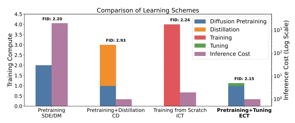
Sampling: One step, or “sculpting” refinement in 2–4 steps In the solver-less extreme, sampling is trivial: draw pure noise \(x_{\sigma _{\max }}\sim \mathcal {N}(0,\sigma _{\max }^2\mathbf {I})\) and feed it to the model once to output \(x_\epsilon \approx f_\theta (x_{\sigma _{\max }},\sigma _{\max })\) [603].
However, a distinctive advantage of CMs is that they are not locked to a single step. We can trade compute for quality at inference without retraining via multistep consistency sampling. If the 1-step output has minor errors or artifacts, we can iteratively refine it through a process of backtracking and jumping again.
The algorithm works in a loop:
- 1.
- The Initial Jump: Get the first guess \(x \approx x_\epsilon \) from pure noise.
- 2.
- The Backtrack (Re-noising): Pick an intermediate noise level \(\tau \) (where \(\epsilon < \tau < \sigma _{\max }\)). We intentionally degrade our guess by adding noise back to it.
- 3.
- The Refinement Jump (Denoising): We feed this newly noisy image back into the model to predict the clean endpoint again.
Mathematically, the re-noising step is defined as:
\begin {equation} \label {eq:chapter20_cm_denoise_renoise} \hat {x}_{\tau } = x + \underbrace {\sqrt {\tau ^2-\epsilon ^2}\,\xi }_{\mbox{Variance Gap}}, \qquad \xi \sim \mathcal {N}(0,\mathbf {I}), \qquad x \leftarrow f_\theta (\hat {x}_\tau ,\tau ). \end {equation}
Understanding the Math (The Variance Gap): Why do we multiply the random noise \(\xi \) by \(\sqrt {\tau ^2-\epsilon ^2}\) instead of just \(\tau \)? Recall that our current guess \(x\) is not perfectly clean; it is an estimate of \(x_\epsilon \), meaning it already contains a tiny residual noise variance of \(\epsilon ^2\). Because variances of independent variables add together, to reach our target total noise variance of \(\tau ^2\), we must only add the difference: \(\epsilon ^2 + (\tau ^2 - \epsilon ^2) = \tau ^2\). This ensures the distribution of \(\hat {x}_\tau \) perfectly matches the expected training distribution at noise level \(\tau \).
Intuition (“Sculpting and Sanding”): Why does destroying the image with noise and decoding it again actually improve it? The 1-step output is like a rough clay cast. It gets the global structure (low frequencies) correct, but the fine details (high frequencies) might be slightly brittle, blurry, or misaligned with the true data manifold. Adding noise acts like sanding: it selectively wipes out those brittle, high-frequency errors while leaving the robust global structure intact. The subsequent decode acts like polishing: the model is given a ”second chance” to hallucinate the fine details, but this time it is starting from a much easier, lower-noise state (\(\tau \)) rather than pure noise (\(\sigma _{\max }\)). Chaining 2 to 4 of these loops corrects local errors efficiently.
Extension: Latent Consistency Models (LCM) and the CFG Tax Running a massive U-Net on a high-resolution pixel grid (e.g., \(1024 \times 1024\)) is incredibly slow, even for just a few steps. Latent Consistency Models (LCM) [416] solve this by migrating the consistency objective into the compressed latent space of text-to-image foundation models like Stable Diffusion. Instead of teleporting pixels \(f_\theta (x_\sigma ,\sigma )\to x_\epsilon \), LCMs teleport latents: \(f_\theta (z_\sigma ,\sigma )\to z_\epsilon \).
Why does it work in latent space? A pretrained Variational Autoencoder (VAE) compresses images into a dense, lower-dimensional semantic space (\(z\)). This space strips away high-frequency pixel noise (exact textures, tiny lighting shifts) and organizes the data mathematically based on core features. Because the latent space is smoother and more perceptually structured than raw pixels, the Probability Flow ODE trajectories inside it are inherently less chaotic. Learning a direct mapping to the origin is actually easier for the network here than in the highly variant pixel space.
The Problem: The “Double Step” CFG Inference Tax Moving to text-to-image models introduces a massive new bottleneck: Classifier-Free Guidance (CFG). To make a standard diffusion model listen to a text prompt (e.g., ”A photograph of a cat”), the generation process relies on CFG. Left to their own devices, diffusion models tend to generate safe, generic images. CFG forces the image to tightly align with the prompt by calculating two separate directional vectors at every single noise level during inference:
- 1.
- The Conditional Pass (\(v_{\mbox{cond}}\)): The network is evaluated with the text prompt (pointing toward ”cat”).
- 2.
- The Unconditional Pass (\(v_{\mbox{uncond}}\)): The network is evaluated without the text prompt using an empty string (pointing toward a generic image).
The numerical solver then extrapolates the final trajectory by pushing away from the generic image and heavily towards the prompt. This extrapolation is controlled by a scale parameter \(\omega \) (e.g., \(\omega = 7.5\)): \[ v_{\mbox{final}} = v_{\mbox{uncond}} + \omega \cdot (v_{\mbox{cond}} - v_{\mbox{uncond}}) \]
The Inference Tax: Because the solver must run the massive neural network twice to take a single step, generating an image in 50 steps at inference actually requires 100 network evaluations (NFE = 100). This 2x compute multiplier is the primary bottleneck for real-time text-to-image generation.
The Solution: Guided Consistency Distillation LCMs achieve extreme speed by shifting this compute tax away from the user’s inference time and entirely onto the training time. They mathematically bake the CFG extrapolation directly into the student model’s weights. Here is exactly how the distillation loop achieves this:
- Phase 1: The Teacher pays the tax (During Training). To teach the student, the frozen teacher model (e.g., Stable Diffusion) must carve out the “true” guided path. It is given a noisy latent \(z_{\sigma _{n+1}}\), a text prompt \(c\), and a randomly chosen CFG scale \(\omega \). The teacher performs the heavy double-evaluation math (Eq. above) and takes a highly accurate, tiny solver step along that extrapolated vector. This produces a slightly cleaner target point \(\hat {z}_{\sigma _n}\). Intuition: This target point is a physical coordinate in latent space. Because the teacher used CFG to get there, the CFG “push” is now permanently baked into the geometry of that coordinate.
- Phase 2: The Student learns the shortcut (During Training). The LCM student model is asked to jump directly to the endpoint of this CFG-baked trajectory. But there is a catch: if the trajectory changes depending on how strong the CFG scale \(\omega \) is, how does the student know where to jump? The Breakthrough: The student model’s architecture is slightly modified to take the CFG scale \(\omega \) as an explicit input parameter alongside the text prompt and the noise level. It learns a direct mapping \(f_\theta (z_\sigma , c, \omega , \sigma )\). Intuition: The student acts as a trajectory memorizer. It learns: “Given this starting noise, this text prompt, and a CFG strength of 7.5, where exactly does the teacher’s path eventually land?”.
- Phase 3: The Ultimate Reward (During Inference). When deployed to a user, the LCM student does not do CFG extrapolation. It does not run an unconditional pass. You simply feed it the starting noise, the text \(c\), and your desired CFG scale \(\omega \). Because it was trained to output the CFG-adjusted destination directly for any given \(\omega \), it predicts the final guided endpoint in a single forward pass. The 2x compute tax is instantly eliminated, drastically multiplying generation speed.
Intuition (“Teleporting the Blueprint”): If a standard pixel-space Consistency Model is like teleporting a finished building brick-by-brick, an LCM is like teleporting the blueprint.
- 1.
- The Math Space (Latent): The network does all its iterative jumps in this tiny, smooth blueprint space.
- 2.
- The Rendering Space (Pixel): Once we possess the perfectly clean blueprint (\(z_\epsilon \)), we hand it to the VAE decoder (\(\mathcal {D}(z_\epsilon ) \approx x_0\)), which renders the high-resolution image.
Crucially, the heavy VAE decoder is only run once at the very end of the process, rather than at every step. By doing the few-step transport in latent space and decoding only once at the end, LCMs substantially reduce inference-time compute relative to pixel-space multi-step samplers, especially at higher output resolutions.
Takeaway Rectified Flow says: “Fix the road so it is easier to drive”. Consistency Models say: “Forget the road; learn the destination map”. Achieving NFE \(\approx 1\) hinges on three ingredients:
- Time-invariance: enforcing self-consistency along ODE trajectories (Eq. 20.119).
- Boundary anchoring: the zipper parameterization at \(\sigma =\epsilon \) (Eq. 20.120).
- A perceptual metric: often LPIPS, to discourage perceptually averaged solutions in the few-step regime [800, 603].
Enrichment 20.11.18: Adversarial Diffusion Distillation (ADD)
Motivation: The 1-Step Barrier and the Need for an Adversary As generative modeling has matured, the field has developed powerful paradigms to accelerate sampling. Broadly, these fall into two categories: simplifying the generative trajectory (e.g., Flow Matching and Rectified Flow) or bypassing the step-by-step solver entirely to learn a direct mapping to the endpoint (e.g., Consistency Models). However, achieving true, high-fidelity one-step generation reveals a fundamental limitation shared by purely regression-based or purely ODE-based methods.
To understand why an adversarial objective becomes important at \(N=1\), we must look at where these existing paradigms fall short:
- The Integration Tax (Flow-Based Methods): Objectives like Rectified Flow aim to straighten the probability path between noise and data so that solving the induced ODE becomes easier. Architectures such as Scalable Interpolant Transformers (SiT) provide a flexible Transformer family for learning interpolant-based generative dynamics (including flow-matching-style objectives), but the paradigm still produces a continuous-time vector field that must be integrated at sampling time. In the strict \(N=1\) regime, taking a single, giant Euler step generally incurs discretization drift: any residual curvature or stiffness of the learned trajectory gets converted into missing or distorted high-frequency detail. Thus, while these methods can be extremely fast, faithful synthesis typically still benefits from \(N\ge 2\) function evaluations.
- The Regression Trap (Consistency Models): Consistency Models learn a direct mapping that bypasses explicit ODE solvers by enforcing that predictions at different noise levels agree under a chosen metric (often perceptual, e.g., LPIPS). In the extreme \(N=1\) setting, the model must map an almost uninformative input (near pure noise) to a detailed image. Under any regression-style metric, the learner is incentivized to produce a safe output that reduces expected error across many plausible completions; this manifests as mode averaging in fine-scale structure, washing out micro-texture into “waxy” / blurry surfaces. Despite this limitation at one step, CMs remain highly attractive in the few-step regime because they provide a deterministic, solver-free sampling interface with strong stability and excellent quality at \(N\approx 2\)–\(8\).
Adversarial Diffusion Distillation (ADD) [567] was explicitly designed to break this regression limit by hybridizing diffusion distillation with a GAN-style discriminator.
Instead of relying solely on regression to find the endpoint, ADD employs a division of labor: a frozen diffusion teacher provides semantic and compositional grounding (ensuring the model respects the prompt and the trajectory structure), while the adversarial signal mathematically penalizes the blurry average. Because a waxy, averaged image is easily detected as “fake”, the discriminator forces the student model to abandon the safe conditional mean and confidently collapse into a single sharp, photorealistic mode.
Competitors or Allies? Initially, CMs and ADD emerged as competing philosophies for few-step generation. ADD is the clear perceptual winner for strict 1-step synthesis, forming the core training paradigm behind extremely fast variants like SDXL-Turbo. However, because adversarial objectives are notoriously unstable to optimize, CMs remain highly competitive at 4–8 steps, where the generation uncertainty drops and the regression blur naturally diminishes.
Today, the community recognizes these approaches as complementary and often combines step-compression objectives with adversarial refinement. For example, SDXL-Lightning combines progressive distillation with an adversarial objective to balance quality and mode coverage, while Hyper-SD builds on consistency-style distillation (trajectory segmentation) and incorporates adversarial weighting to improve low-step realism [365, 542].
Setup: Teacher vs. Student schedules (Baby steps vs. Giant leaps) Let a pretrained diffusion model (the teacher) be defined on a dense time grid \(t\in \mathcal {T}_{\mbox{teacher}}=\{0,1,\dots ,T\}\) with \(T=1000\), where \(t=T\) corresponds to (approximately) pure noise and \(t=0\) corresponds to clean data. ADD trains a student denoiser on a drastically reduced set of steps \(\mathcal {T}_{\mbox{student}}=\{\tau _1,\dots ,\tau _n\}\) with \(\tau _n = T\) and typically \(n\in \{1,2,4\}\).
Using standard diffusion notation, we form the student’s noisy input at step \(s\): \begin {equation} \label {eq:chapter20_add_forward} \mathbf {x}_s = \underbrace {\alpha _s \mathbf {x}_0}_{\mbox{Signal}} + \underbrace {\sigma _s \boldsymbol {\epsilon }}_{\mbox{Noise}}, \qquad \boldsymbol {\epsilon }\sim \mathcal {N}(\mathbf {0},\mathbf {I}), \qquad s\in \mathcal {T}_{\mbox{student}}. \end {equation} Intuition: The coefficients \(\alpha _s\) and \(\sigma _s\) control the Signal-to-Noise Ratio (SNR). At the start of generation (\(s=\tau _n\)), the signal is completely destroyed (\(\alpha _s \approx 0, \sigma _s \approx 1\)). The student is tasked with producing a fully denoised estimate \(\hat {\mathbf {x}}_\theta (\mathbf {x}_s,s)\) from this pure noise in a single massive jump, effectively skipping hundreds of the teacher’s intermediate waypoints.
Latent diffusion instantiation (The SDXL Architecture). Although ADD is often written in “image space” (\(\mathbf {x}\)) for notational simplicity, modern foundation models like Stable Diffusion and SDXL operate in a compressed latent space. Concretely, a high-resolution RGB image \(\mathbf {x}_0\in \mathbb {R}^{3\times 1024\times 1024}\) is first compressed by a Variational Autoencoder (VAE) into a denser, lower-dimensional latent representation \(\mathbf {z}_0\in \mathbb {R}^{4\times 128\times 128}\). The noise addition (Eq. 20.124) and the student’s denoising prediction both occur entirely within this mathematically smoother latent space, predicting \(\hat {\mathbf {z}}_\theta (\mathbf {z}_s,s)\).
The Backpropagation Bottleneck: This latent architecture creates a severe engineering friction point for ADD. The student predicts latents (\(\hat {\mathbf {z}}_\theta \)), but the ADD discriminator (powered by DINOv2) is designed to evaluate raw RGB pixels (\(\hat {\mathbf {x}}_\theta \)). To compute the adversarial loss during training, the student’s predicted latents must be actively decoded through the VAE decoder network at every single training step (\(\hat {\mathbf {x}}_\theta = \mathcal {D}(\hat {\mathbf {z}}_\theta )\)).
More problematically, to actually update the student’s weights, the gradient calculated by the discriminator must backpropagate all the way through the massive convolutional layers of the VAE decoder before it finally reaches the student. This forces the training loop to store enormous high-resolution activation tensors in GPU memory for every image in the batch. This drastically throttles training speed, limits feasible batch sizes, and creates the central compute bottleneck that directly motivated the development of latent-space variants like LADD.
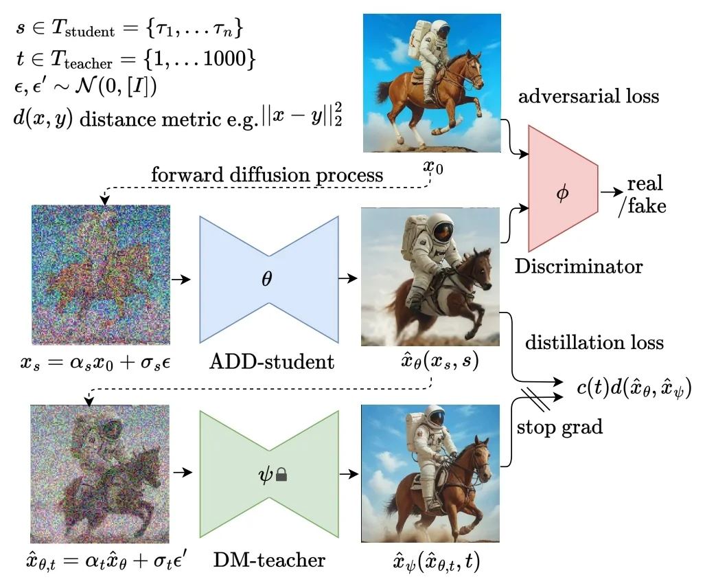
The two objectives: distill the teacher, sharpen with a discriminator ADD optimizes a distillation loss and an adversarial loss simultaneously. The teacher supplies a trajectory-consistent target (preventing semantic drift and structural hallucinations), while the discriminator supplies the high-frequency realism prior that regression struggles to provide at one step.
Distillation loss: teacher denoising targets with stop-gradient A naive approach to distillation might be to simply ask the teacher to critique the student’s generated image \(\hat {\mathbf {x}}_\theta \) directly. However, ADD defines the teacher-generated target by first re-noising the student’s current prediction to a randomly selected teacher time \(t\in \mathcal {T}_{\mbox{teacher}}\): \begin {equation} \label {eq:chapter20_add_renoise} \hat {\mathbf {x}}_{\theta ,t} = \alpha _t \hat {\mathbf {x}}_\theta (\mathbf {x}_s,s) + \sigma _t \boldsymbol {\epsilon }', \qquad \boldsymbol {\epsilon }'\sim \mathcal {N}(\mathbf {0},\mathbf {I}). \end {equation}
Why re-noise? (The Out-of-Distribution Problem). The teacher is trained to denoise diffused inputs across a noise schedule. Feeding a non-diffused student output directly to the teacher is out-of-distribution, so the resulting correction signal can be unreliable [567]. The teacher is trained to denoise diffused inputs; applying it directly to a non-diffused student output is out-of-distribution for the teacher, so the resulting correction signal is unreliable [567].
By actively injecting noise \(\sigma _t \boldsymbol {\epsilon }'\), we submerge the student’s flawed prediction back into the noisy probability flow where the teacher is an expert. The teacher looks at this newly noisy state \(\hat {\mathbf {x}}_{\theta ,t}\) and asks: “If I were at this exact coordinate, what clean image would I predict?”. Because the teacher is highly robust to noise, its denoised prediction naturally “projects” the weird, five-legged dog back onto the nearest valid point on the true data manifold (a normal, four-legged dog).
The frozen teacher denoiser \(\hat {\mathbf {x}}_\psi (\cdot ,t)\) then produces this ideal denoised target \(\hat {\mathbf {x}}_\psi (\hat {\mathbf {x}}_{\theta ,t},t)\), and the student is trained to match it using a weighted \(\ell _2\) distance: \begin {equation} \label {eq:chapter20_add_distill} \mathcal {L}_{\mbox{distill}} = \mathbb {E}_{\mathbf {x}_0,\boldsymbol {\epsilon },\boldsymbol {\epsilon }',\,s,t} \Big [ c(t)\,d\!\Big ( \hat {\mathbf {x}}_\theta (\mathbf {x}_s,s), \operatorname {stopgrad}\big (\hat {\mathbf {x}}_\psi (\hat {\mathbf {x}}_{\theta ,t},t)\big ) \Big ) \Big ], \qquad d(\mathbf {x},\mathbf {y}) \equiv \|\mathbf {x}-\mathbf {y}\|_2^2. \end {equation}
Stop-gradient intuition: The teacher acts strictly as a frozen, immovable critic. We never backpropagate through the parameters in the teacher network to make it compromise with the student. We only use its output as a fixed coordinate in image space, generating a direct error signal that updates solely the student’s weights.
Why is \(\ell _2\) not “too strict” here? Because the teacher’s target might slightly shift pixels (e.g., moving a strand of hair to a more ”natural” position), using a pixel-perfect \(\ell _2\) metric might intuitively seem like it would punish the student unfairly, forcing it to hedge its bets and blur the image. If \(\ell _2\) were the only objective, this regression to the mean would absolutely occur.
However, in the ADD hybrid framework, \(\mathcal {L}_{\mbox{distill}}\) is not responsible for teaching textures. It acts purely as a structural leash. The \(\ell _2\) distance forms a directional vector pointing directly from the student’s GAN-hallucinated structure toward the nearest structurally sound, prompt-aligned layout known by the teacher. The adversarial loss simultaneously pushes back against the texture-smoothing tendency of this \(\ell _2\) penalty. This yields a precise equilibrium: the global geometry and prompt adherence follow the teacher’s structural leash, while the crisp, high-frequency realism is strictly enforced by the discriminator.
Adversarial loss: a projected discriminator on frozen semantic features (DINOv2) To push sharpness and realism, ADD trains a discriminator \(D_\phi \) to distinguish real images \(\mathbf {x}_0\) from generated samples \(\hat {\mathbf {x}}_\theta (\mathbf {x}_s,s)\) with a hinge-style GAN objective [567].
A crucial stabilization trick is that \(D_\phi \) is not a standard convolutional network trained from scratch on raw pixels. Standard GANs are notoriously unstable and easily fooled by high-frequency artifacts (like checkerboard patterns) because the discriminator and generator are learning simultaneously. Instead, ADD uses a projected GAN discriminator: it is built on top of a massive, frozen, pretrained visual backbone \(\Phi (\cdot )\) (a Vision Transformer trained self-supervised, typically DINOv2 [477]). Because DINOv2 provides strong pretrained semantic features, the projected discriminator becomes harder to exploit via trivial pixel-level artifacts and yields a substantially more stable and informative training signal in the low-step regime [567, 477]. Lightweight trainable heads \(D_{\phi ,k}\) are attached to the intermediate features of this frozen backbone: \[ D_\phi (\mathbf {x},\mathbf {c}) = \sum _k D_{\phi ,k}\big (\Phi _k(\mathbf {x}),\mathbf {c}\big ), \] where \(\mathbf {c}\) denotes conditioning (e.g., a text embedding; making this a projection discriminator).
The \(\ell _2\) vs. LPIPS Debate: Why ADD reduces the need for a separate perceptual regression loss. In standard distillation frameworks (like Consistency Models), using a pure \(\ell _2\) (Mean Squared Error) pixel loss is disastrous; it averages modes and creates waxy, blurry images.
To combat this, standard CMs heavily rely on LPIPS (Learned Perceptual Image Patch Similarity) for their distance metric, which calculates errors in the feature space of a pretrained VGG network to preserve perceptual sharpness.
So why does ADD’s distillation loss (\(\mathcal {L}_{\mbox{distill}}\)) revert to using basic, computationally cheap \(\ell _2\) distance? The answer lies in the DINOv2 discriminator. The projected discriminator effectively acts as an immensely powerful, dynamically trained perceptual loss.
- Redundancy: LPIPS uses a VGG network to judge high-level features. The ADD discriminator uses DINOv2 to do the exact same thing, but with a vastly superior, modern semantic understanding.
- Strict Division of Labor: Adding LPIPS on top of the distillation loss would be computationally wasteful and mathematically redundant. The cheap \(\ell _2\) loss serves primarily as a structural leash, while the adversarial loss supplies the perceptual pressure that would otherwise motivate LPIPS in purely regression-based distillation [567].
What goes in, what comes out, and how the student learns. The discriminator evaluates two streams—real images (\(\mathbf {x}_0\)) and fake generated images (\(\hat {\mathbf {x}}_\theta \))—passing both through the frozen DINOv2 backbone. The feature maps are extracted at multiple depths:
- Shallow features capture edges, lighting, and high-frequency textures (e.g., fur, skin pores).
- Deep features capture global anatomy and object-level semantics (e.g., does this dog have the correct number of legs?).
Each small head outputs a realness score for its specific depth. The hinge loss combines these scores and calculates the gradient. Crucially, the discriminator does not just output a binary “fake” label. It supplies a dense, feature-aware vector field via backpropagation. It tells the student exactly which pixels to push, and in what direction, to reconstruct the specific textures and anatomical structures that DINOv2 recognizes as photorealistic.
Image conditioning (Encouraging use of the input signal). For intermediate student steps \(\tau <1000\), the ADD-student input \(\mathbf {x}_s=\alpha _s\mathbf {x}_0+\sigma _s\boldsymbol {\epsilon }\) still contains information about the originating clean image \(\mathbf {x}_0\). ADD exploits this by conditioning the discriminator not only on text (projection), but also on an image embedding \(c_{\mbox{img}}\) extracted from \(\mathbf {x}_0\). Intuitively, this encourages the student to utilize the input signal effectively (rather than ignoring it and only optimizing unconditional realism), and empirically the combination of text and image conditioning yields the best results [567].
Overall training objective and the pixel–latent split (The VAE Bottleneck) The full training objective combines these two forces into a single weighted sum: \begin {equation} \label {eq:chapter20_add_total} \mathcal {L}_{\mbox{ADD}} = \mathcal {L}_{\mbox{distill}} + \lambda _{\mbox{adv}}\,\mathcal {L}_{\mbox{adv}} \;+\; \mbox{(regularization, e.g., R1)}. \end {equation}
The hyperparameter \(\lambda _{\mbox{adv}}\) is the critical dial that balances the equilibrium: too low, and the model collapses back to the waxy regression mean; too high, and the GAN discriminator overpowers the structural leash, causing geometric hallucinations.
The Pixel–Latent Split and the Memory Crisis. When instantiating ADD with a latent diffusion model (e.g., SDXL), the teacher and student denoisers operate natively in latent space. However, ADD formulates the training losses in pixel space: for LDMs with a shared latent space, the distillation loss could be computed in latent or pixel space, and ADD reports using pixel-space distillation because it yields more stable gradients [567]. Since the adversarial objective is also pixel-based, training repeatedly decodes predicted latents to RGB, \(\hat {\mathbf {x}}_\theta =\mathcal {D}(\hat {\mathbf {z}}_\theta )\), making VAE decoding (and backpropagation through it) the dominant compute and VRAM bottleneck.
To update the student’s weights, feature-aware gradients must backpropagate all the way through the massive, heavily parameterized convolutional layers of the VAE decoder just to reach the student’s U-Net. Because modern autograd engines must store intermediate activation tensors for the entire high-resolution pixel grid (e.g., \(3 \times 1024 \times 1024\)), VRAM consumption explodes. This forces engineers to use tiny batch sizes or restrict training resolutions entirely.
This exact throughput bottleneck is the direct motivation for the next generation of adversarial distillation: latent-space variants (such as LADD) that evaluate the adversarial game strictly within the compressed boundary of the latents.
Choice of Teacher and Student: Why Multistep is Mandatory A natural question arises regarding the prerequisites for the networks involved in this distillation process. What kind of model qualifies to be the teacher, and where does the student start?
- The Teacher (Dense-time denoiser): The teacher must provide reliable denoising predictions at arbitrary timesteps \(t\in \mathcal {T}_{\mbox{teacher}}\) so that the student prediction can be re-noised to \(t\) and “critiqued” via the teacher target. In practice, this is naturally satisfied by a standard pretrained diffusion model (e.g., SDXL), which is trained to denoise across a dense noise schedule and thus can serve as a dependable “compass” throughout the trajectory [567].
- The Student (The Pretrained Clone): The student model utilizes the exact same architecture as the teacher (e.g., a massive U-Net or DiT). Crucially, the student is initialized with the teacher’s pretrained weights rather than starting from random initialization. Training a GAN from scratch to generate photorealistic megapixel images in one step is notoriously unstable and almost guarantees catastrophic mode collapse. By inheriting the teacher’s weights, the student begins the distillation process with a profound, preexisting semantic understanding of the data manifold. It already knows how to render complex textures and anatomy; the adversarial training simply acts as an aggressive curriculum, forcing the student to compress that iterative knowledge into a single, confident jump.
Fast sampling and refinement: one step vs. a few steps Although ADD is heavily marketed as a 1-step generator (and achieves state-of-the-art results doing so), it natively remains a conditional diffusion denoiser \(\hat {\mathbf {x}}_\theta (\mathbf {x}_s,s)\). This means it is entirely compatible with multi-step sampling by chaining predictions along its reduced schedule \(\mathcal {T}_{\mbox{student}}\).
The Intuition: “Drafting and Polishing”. Think of the generation process as a sculptor blocking out a statue before chiseling the fine details.
- Step 1 (The Draft): When evaluating from near-pure noise (\(s=\tau _n\)), the model faces maximum mathematical uncertainty. It must perform the heavy lifting of resolving the global semantics—hallucinating the composition, spatial layout, and major objects out of pure static. While the adversarial loss ensures this “first draft” is sharp rather than blurry, the sheer difficulty of the 1-step jump means that highly complex prompt constraints or micro-details (like perfect facial symmetry or rendering text) might be slightly brittle.
- Steps 2–4 (The Polish): If we want higher quality, we perform iterative refinement by running the same student denoiser on its reduced schedule across 2–4 discrete noise levels. We take the 1-step output, add a small, calibrated amount of noise back to it, and feed it through the model again at a lower noise level (\(\tau _{n-1}\)). Because the injected noise is small, the global layout remains locked in place, and the model can focus on local corrections and texture refinement.
Thus, moving from 1 step to 2–4 steps enables a fast “explore-then-refine” workflow: users can rapidly generate 1-step seeds at zero latency to find a composition they like, and then allocate 4 steps to polish that specific layout into a final, high-fidelity image without the composition drastically changing.
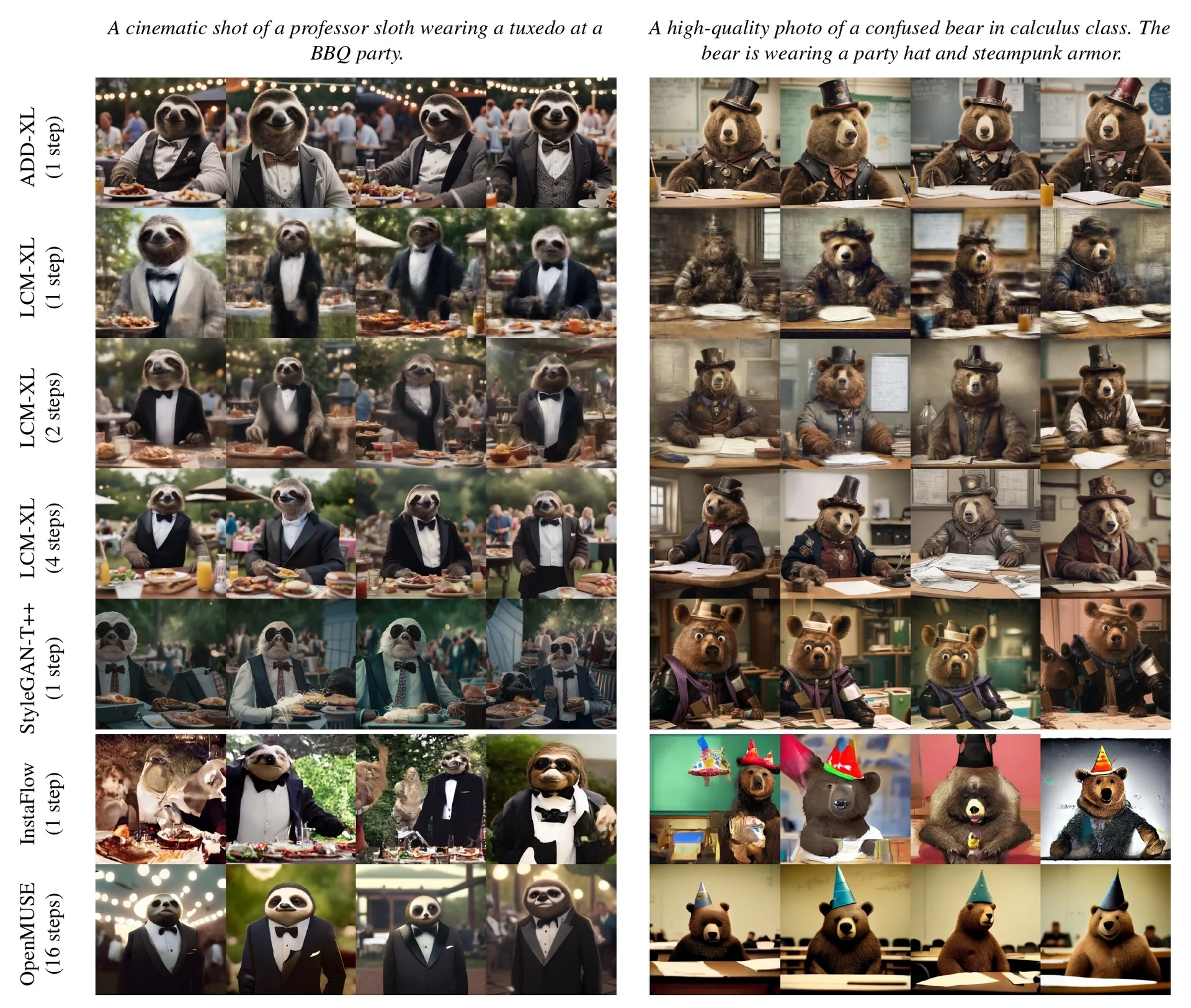
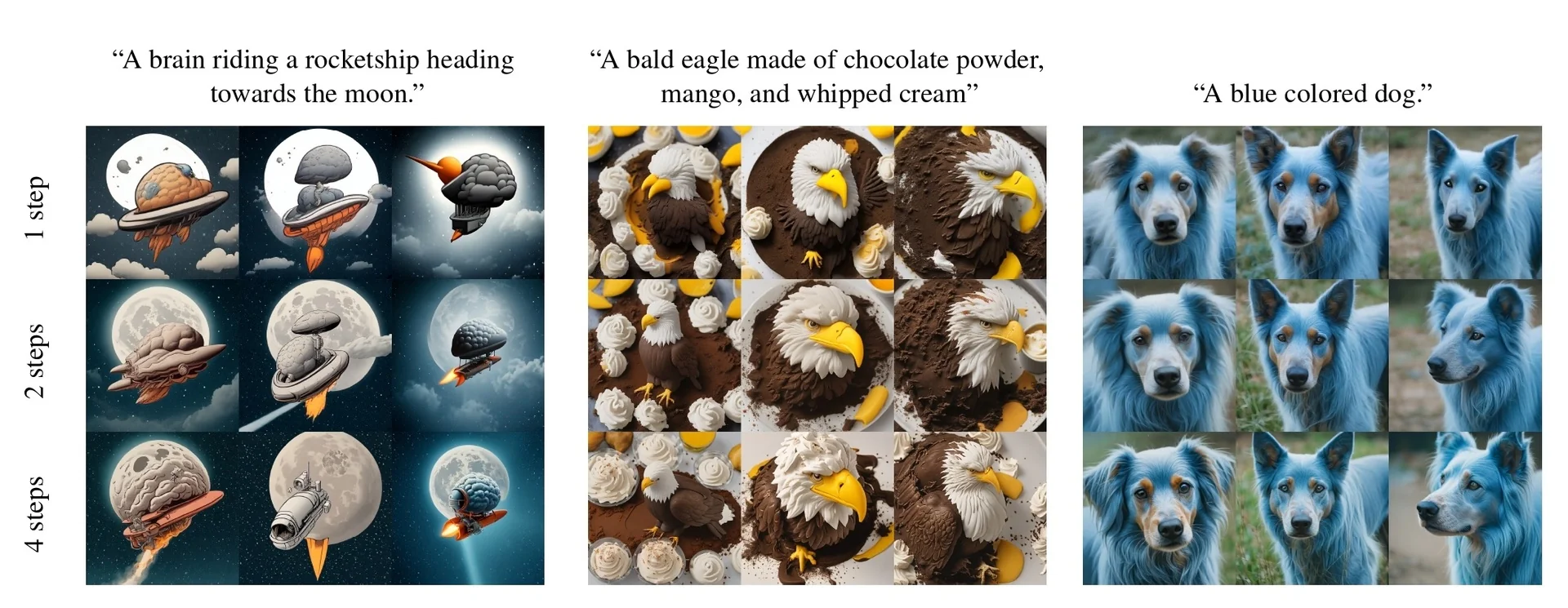
Key experiments and ablations: what actually matters? ADD validates its design via controlled ablations that isolate discriminator design, conditioning, and the balance between distillation and adversarial losses [567]. The most important takeaways are:
- Both losses are necessary. \(\mathcal {L}_{\mbox{adv}}\) alone degrades quality, while \(\mathcal {L}_{\mbox{distill}}\) alone fails catastrophically; the hybrid objective is essential for stable, high-fidelity 1-step synthesis.
- A strong frozen feature backbone matters. DINOv2 features in the discriminator outperform alternative feature networks; random initialization collapses, indicating the discriminator must provide semantic gradients, not only local texture cues.
- Conditioning helps, especially jointly. Text conditioning improves prompt alignment; adding image conditioning improves fidelity; combining both yields the best overall trade-off.
- Initialization is critical. Initializing the student from a pretrained diffusion model is necessary; training from scratch fails, consistent with the hardness of 1-step generation.
Can the student beat the teacher? (texture vs. diversity) A striking qualitative result is that ADD-XL can appear more realistic than its SDXL teacher on texture-heavy regions (fur, fabric, skin), consistent with the discriminator penalizing diffusion-style oversmoothing. The trade-off is a tendency toward reduced diversity compared to the teacher, a common side effect of GAN training.
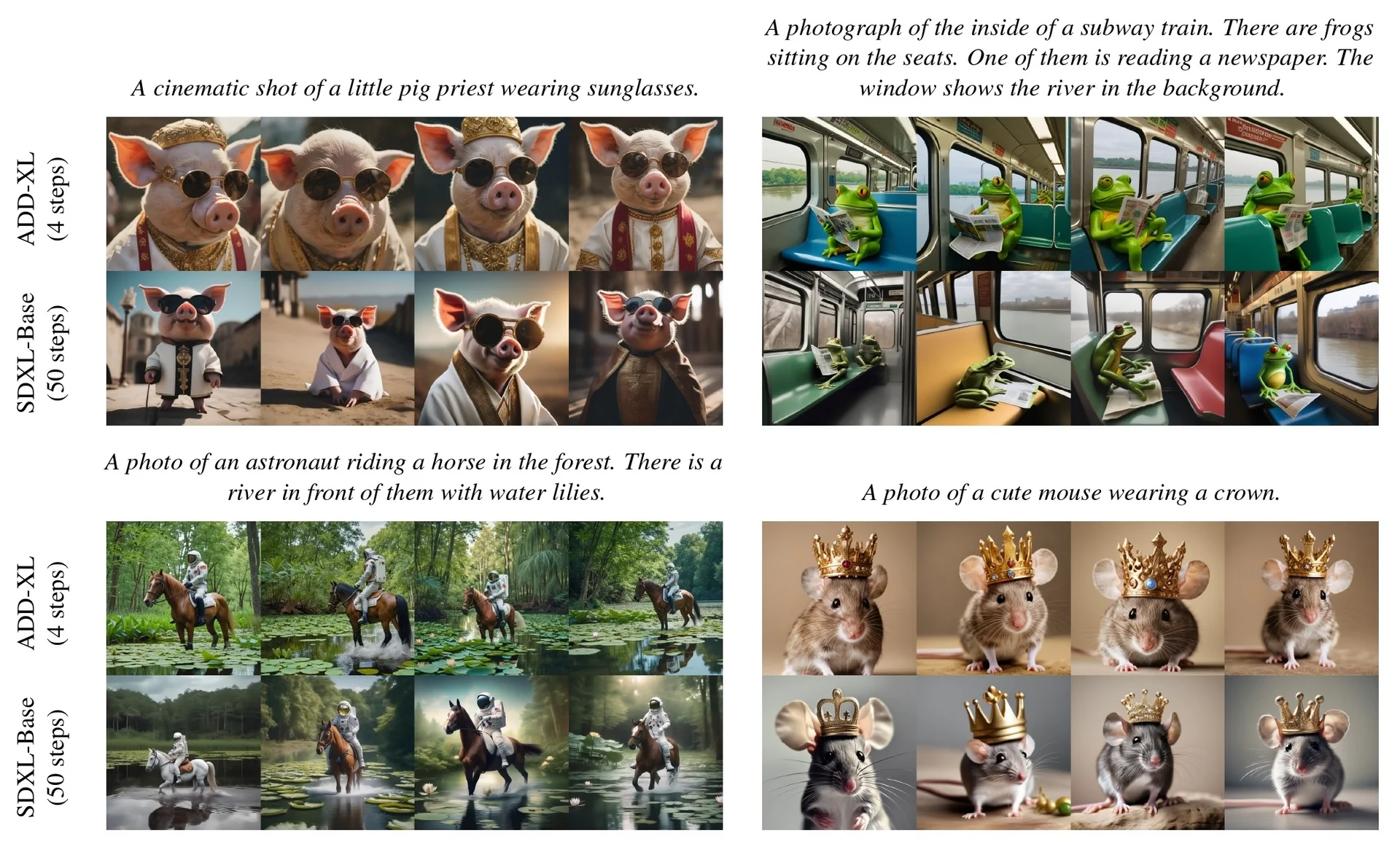
From ADD to LADD and DMD: Removing the Two Bottlenecks ADD was a monumental proof-of-concept: it demonstrated that adversarial realism can be successfully distilled into a diffusion student, effectively breaking the 1-step blurriness barrier. However, treating ADD as a production-ready paradigm for next-generation foundation models (like Stable Diffusion 3) exposes two distinct scaling bottlenecks:
- The Pixel/VAE Bottleneck (The Memory Crisis): Because the DINOv2-based discriminator operates exclusively on raw RGB pixels, the training loop is forced to decode the student’s predicted latents into high-resolution images at every single iteration (\(\mathcal {D}(\hat {\mathbf {z}}_\theta ) \to \hat {\mathbf {x}}_\theta \)). Crucially, the adversarial gradients must then backpropagate entirely through the massive convolutional layers of this VAE decoder to reach the student. This consumes an enormous amount of VRAM, strictly limiting training to lower resolutions (e.g., 512px) and making scaling to megapixel or multi-aspect generation computationally prohibitive.
- The GAN Tightrope (The Stability Crisis): Adversarial optimization is not standard loss minimization; it is a delicate, two-player Min-Max game. It depends sensitively on empirical tuning, architecture choices, and precise loss balancing to ensure the discriminator does not overpower the student too quickly (which kills the gradients) or too slowly (which allows artifacts). This reliance on a rigid, external judge makes scaling the distillation process to broader, more complex datasets a mathematically fragile endeavor.
These two severe limitations forced the research community to branch into two complementary directions, each engineered to surgically remove one of these exact bottlenecks:
- LADD (Latent Adversarial Diffusion Distillation) [568] tackles the memory crisis. It removes the VAE decode bottleneck entirely by shifting the adversarial supervision directly into the compressed latent space, utilizing features extracted from the teacher model itself.
- DMD (Distribution Matching Distillation) [759] tackles the stability crisis. It eliminates the discriminator entirely, replacing the volatile GAN game with a mathematically pure, discriminator-free distribution matching objective for 1-step distillation.
To understand how the industry achieved megapixel, 4-step generation on consumer hardware (as seen in SD3-Turbo), we first turn our attention to the architectural bypass of LADD.
Enrichment 20.11.19: Latent Adversarial Diffusion Distillation (LADD)
Motivation: Fixing ADD’s Pixel Bottleneck Without Giving Up Adversarial Sharpness Adversarial Diffusion Distillation (ADD) demonstrates that a GAN-style discriminator can break the one-step “regression-to-the-mean” barrier by explicitly penalizing oversmoothed, low-texture outputs [567]. However, when ADD is instantiated on latent diffusion models, its adversarial branch remains pixel-bound: the discriminator consumes RGB images, so the student must decode latents through the VAE at every training step. This repeated decoding (and backpropagation through it) becomes a dominant throughput and VRAM bottleneck, effectively hard-capping scalable high-resolution and multi-aspect ratio training.
Latent Adversarial Diffusion Distillation (LADD) [568] removes this bottleneck by moving the entire adversarial game into latent space. The key unification is conceptual: instead of using an external discriminative feature backbone (e.g., DINOv2) on pixels, LADD uses the frozen generative teacher itself as the feature extractor for a projected GAN loss, so no pixel decoding is required. In addition, because the teacher features depend on the noise level, LADD can explicitly control whether the discriminator emphasizes global coherence (high noise) or fine texture (low noise), and can naturally support multi-aspect ratio (MAR) training by reshaping token features back into 2D grids [568].
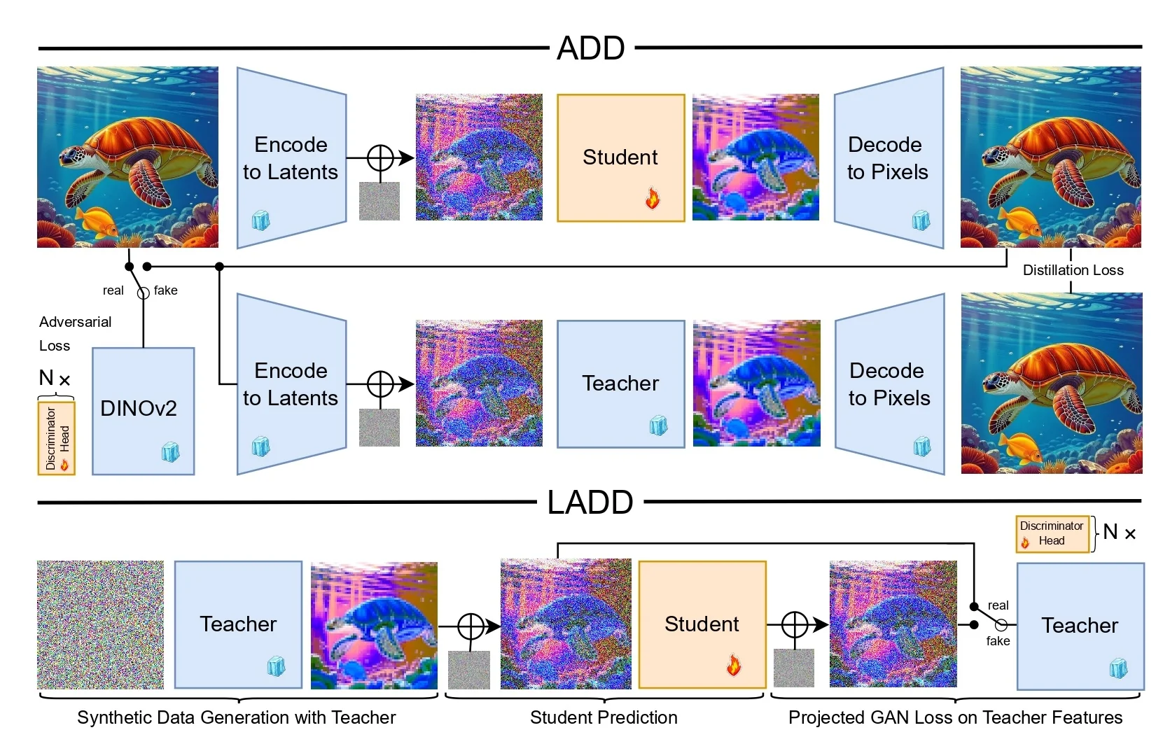
Setup: Synthetic Ground Truth and When Distillation Becomes Unnecessary A central practical challenge for adversarial distillation is prompt alignment. Natural image–text datasets can exhibit weak or noisy alignment, so an adversarially trained student can drift toward sharp but poorly conditioned samples unless anchored by an auxiliary distillation objective (as in ADD).
LADD takes a different route: it manufactures highly aligned supervision by generating the training data using the frozen teacher itself at a fixed classifier-free guidance (CFG) value [568]. Concretely, for a prompt (and its text embedding) \(\mathbf {c}\), the teacher produces a clean latent \[ \mathbf {z}_{\mbox{real}} \in \mathbb {R}^{C \times h \times w}. \] Since the training pairs are now teacher-generated, image–text alignment is substantially improved and comparatively uniform. Empirically, LADD finds that while an auxiliary distillation loss can help when training on real data, it offers no advantage when training on synthetic teacher-generated data; thus, synthetic-data training can be performed using only an adversarial loss [568].
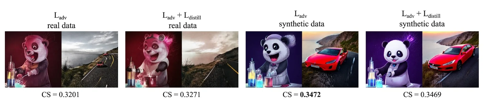
Method: The LADD Training Scheme and Latent Rectified Flow LADD migrates the ADD adversarial game fully into latent space by unifying the teacher and the discriminator pipeline: the teacher not only generates aligned synthetic training latents, but also provides the internal generative features on which adversarial realism is judged [568]. This removes the pixel-space VAE decode bottleneck and (when training on synthetic data) makes an explicit ADD-style distillation loss unnecessary.
High-Level Overview (Three Actors). LADD’s training loop has a strict frozen/trainable split:
- 1.
- Teacher model \(T\): Frozen. A pretrained latent diffusion / rectified-flow teacher (e.g., SD3). It (i) generates synthetic, prompt-aligned latents \(\mathbf {z}_{\mbox{real}}\) and (ii) acts as a fixed feature extractor whose intermediate representations define the adversarial signal.
- 2.
- Student model \(D_\theta \): Trainable. A fast denoiser that maps noisy latents to a clean latent in \(1\)–\(4\) steps.
- 3.
- Discriminator heads \(\{h_{\phi ,k}\}\): Trainable. Lightweight 2D convolutional heads attached to features extracted from teacher blocks \(k\), trained to classify teacher features from \(\mathbf {z}_{\mbox{real}}\) as real and features induced by the student as fake.
Step 1: Forward corruption (rectified-flow parameterization). Rather than a discrete DDPM variance schedule, LADD uses a continuous-time interpolation \(t\in [0,1]\), where \(t=1\) denotes pure Gaussian noise and \(t=0\) denotes clean data. Given a teacher-generated clean latent \(\mathbf {z}_{\mbox{real}}\) and a sampled \(t\), the corruption path is the straight line \begin {equation} \label {eq:chapter20_ladd_forward} \mathbf {z}_t = (1-t)\,\mathbf {z}_{\mbox{real}} + t\,\boldsymbol {\epsilon }, \qquad \boldsymbol {\epsilon }\sim \mathcal {N}(\mathbf {0},\mathbf {I}). \end {equation} Intuition: the model is trained on a geometrically simple path (a chord) between \(\mathbf {z}_{\mbox{real}}\) and pure noise, so “denoising” becomes learning how to move back along this line.
Step 2: Student prediction (velocity field). The student receives \((\mathbf {z}_t,t)\) and predicts the clean endpoint. LADD parameterizes this via a learned velocity field \(F_\theta \): \begin {equation} \label {eq:chapter20_ladd_student} D_\theta (\mathbf {z}_t,t) \;=\; \hat {\mathbf {z}}_0 \;=\; \mathbf {z}_t - t\,F_\theta (\mathbf {z}_t,t). \end {equation} Intuition (velocity): \(F_\theta \) is a learned “push” that points from the current noisy state back toward the clean manifold; multiplying by \(t\) naturally shrinks the correction near \(t\!\approx \!0\) and enlarges it near \(t\!\approx \!1\). At inference, one can apply \(D_\theta \) once (one-step) or compose it over a small discrete grid (few-step refinement); the paper trains on a small set of discrete timesteps for stability at high resolution [568].
Notation. We use \(t\in [0,1]\) for the student corruption level in Eq. (20.128), and \(\hat {t}\in [0,1]\) for a separate teacher-noise level used only to grade realism in the adversarial loss (Step 3).
Step 3: Renoising for Frequency-Controlled Grading.
After the student predicts a clean latent \(\hat {\mathbf {z}}_0\), LADD does not grade realism only at the clean endpoint (\(\hat {t}\!=\!0\)). Instead, it evaluates teacher features at a chosen noise level \(\hat {t}\), so the adversarial signal can be steered toward either global structure (high \(\hat {t}\)) or fine detail (low \(\hat {t}\)) without ever decoding to pixels [568].
Hence, LADD renoises both the true synthetic latent and the student’s predicted latent at a newly sampled, independent noise level \(\hat {t}\), and evaluates these corrupted versions through the teacher’s features. Concretely, we sample \(\hat {t} \sim \pi (\hat {t}; m, s)\) and form the renoised latents:
\begin {equation} \label {eq:chapter20_ladd_renoise} \tilde {\mathbf {z}}_{\mbox{real}} = (1-\hat {t})\,\mathbf {z}_{\mbox{real}} + \hat {t}\,\boldsymbol {\eta }, \qquad \tilde {\mathbf {z}}_{\mbox{fake}} = (1-\hat {t})\,\hat {\mathbf {z}}_0 + \hat {t}\,\boldsymbol {\eta }', \qquad \boldsymbol {\eta },\boldsymbol {\eta }'\sim \mathcal {N}(\mathbf {0},\mathbf {I}). \end {equation}
To ensure \(\hat {t}\) is smoothly bounded between \(0\) (clean data) and \(1\) (pure noise), we parameterize \(\pi \) as a logit-normal distribution by sampling \(u\sim \mathcal {N}(m,s^2)\) and mapping it through a sigmoid:
\begin {equation} u \sim \mathcal {N}(m, s^2) \quad \Longrightarrow \quad \hat {t} = \operatorname {sigmoid}(u) = \frac {1}{1+e^{-u}} \in (0,1). \end {equation}
Demystifying the \(m\) and \(s\) Parameters. The variables \(m\) (location) and \(s\) (scale) represent the mean and standard deviation of the underlying Gaussian distribution before the sigmoid transformation is applied. They serve as direct control dials for the frequency spectrum the discriminator will process:
- Location (\(m\)): This shifts the center of the distribution. If \(m = 0\), the median of \(u\) is \(0\), and thus the median noise level is \(\operatorname {sigmoid}(0) = 0.5\). If we set \(m > 0\), the distribution skews heavily toward pure noise. For instance, setting \(m = 1\) shifts the median noise level up to \(\operatorname {sigmoid}(1) \approx 0.73\).
- Scale (\(s\)): This controls the spread. A smaller \(s\) concentrates the sampled timesteps tightly around the median, while a larger \(s\) flattens the distribution, pushing more samples toward the extreme boundaries of \(0\) and \(1\) due to the asymptotic tails of the sigmoid function.
Intuition: The Frequency Filter. Renoising turns \(\hat {t}\) into an explicit frequency filter, dictating exactly what structural information survives for the discriminator to “see”.
- High Noise (\(\hat {t} \to 1\)): Micro-textures, sharp edges, and fine details are completely destroyed by the Gaussian noise. The discriminator is forced to look past the static and evaluate only the surviving low-frequency structural skeleton, penalizing errors in global coherence, object proportions, and layout.
- Low Noise (\(\hat {t} \to 0\)): The global structure is obvious and uncorrupted. The discriminator becomes highly sensitive to high-frequency local realism, penalizing waxy textures, blurry edges, and artificial-looking surfaces.
Choosing \(\pi (\hat {t};m,s)\) (coherence–detail trade-off). The teacher-noise distribution directly trades off global coherence against fine detail. If \(\pi (\hat {t};m,s)\) concentrates too much mass near \(\hat {t}\approx 0\), the adversarial signal strongly emphasizes local texture realism, but the model can neglect long-range structure (e.g., inconsistent geometry). Biasing \(\pi \) toward larger \(\hat {t}\) suppresses high-frequency detail in \(\tilde {\mathbf {z}}\) and forces the adversarial heads (through teacher features) to judge what remains: overall layout, proportions, and object-level consistency. However, pushing \(\hat {t}\) too close to \(1\) starves the discriminator of fine-scale information and reduces sharpness. Following the paper, a logit-normal schedule with \((m{=}1,s{=}1)\) provides a robust default, while more extreme biasing (e.g., \((m{=}2,s{=}2)\)) measurably degrades fine detail (see the below figure).
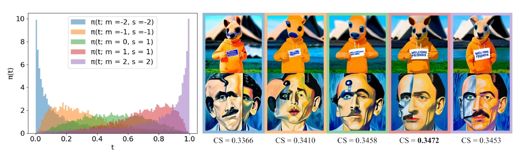
Step 4: Latent Projected GAN on teacher features (alternating updates). After the renoising step, the corrupted latents \(\tilde {\mathbf {z}}_{\mbox{real}}\) and \(\tilde {\mathbf {z}}_{\mbox{fake}}\) are passed forward through the frozen teacher network \(T\). Following the LADD framework, we tap into the frozen teacher and extract intermediate token features after attention blocks; these token sequences are then folded back to a 2D grid before applying the 2D convolutional heads (see the MAR discussion below) [568]. We then attach independent discriminator heads to these extracted features. These heads are additionally conditioned on the teacher-noise level \(\hat {t}\) and pooled CLIP embeddings \(\mathbf {e}\) [568].
Let \(\tilde {\mathbf {F}}^{(k)}_{\mbox{real}}\) and \(\tilde {\mathbf {F}}^{(k)}_{\mbox{fake}}\) denote the teacher features at block \(k\) induced by \(\tilde {\mathbf {z}}_{\mbox{real}}\) and \(\tilde {\mathbf {z}}_{\mbox{fake}}\), respectively.
Note: These features are produced natively as 1D token sequences by the transformer but are reshaped into a 2D spatial grid before applying the 2D convolutional heads; see Eq. (20.135) and the MAR discussion that follows.
Alternating updates. LADD follows standard GAN training practice by alternating between (i) updating the discriminator heads while freezing the student, and (ii) updating the student while freezing the heads. This prevents the critic and generator from drifting simultaneously and yields a stable training signal in the projected (teacher-feature) space [568].
To solve this, LADD uses an alternating optimization loop. During every single training iteration (i.e., for every batch of data), the system freezes one part of the network while training the other, and then immediately swaps their roles. This creates a two-phase ”cat-and-mouse” game: Phase A teaches the critic how to judge, and Phase B teaches the student how to fool the newly updated critic.
Hinge losses. To formalize this game, LADD employs the hinge loss formulation. Define:
\begin {equation} \label {eq:chapter20_ladd_hinge} \ell _{\mbox{D}}(a_{\mbox{real}},a_{\mbox{fake}}) = \max (0,\,1-a_{\mbox{real}}) + \max (0,\,1+a_{\mbox{fake}}), \qquad \ell _{\mbox{G}}(a_{\mbox{fake}})=-a_{\mbox{fake}}. \end {equation} Intuitively, \(\ell _{\mbox{D}}\) forces the discriminator to push the scores of real features (\(a_{\mbox{real}}\)) above \(+1\) and fake features (\(a_{\mbox{fake}}\)) below \(-1\). The generator’s loss \(\ell _{\mbox{G}}\) simply tries to push the fake scores as high as possible.
Phase A: The Critic’s Turn (Update discriminator heads \(\phi \)).
- When: The first half of the training iteration.
- How: The weights of the student model \(\theta \) and the teacher \(T\) are strictly frozen. We feed both the real features \(\tilde {\mathbf {F}}^{(k)}_{\mbox{real}}\) and the fake features \(\tilde {\mathbf {F}}^{(k)}_{\mbox{fake}}\) into the discriminator heads \(\phi \). The heads calculate their scores, and the gradients are backpropagated only into the discriminator’s parameters.
Mathematically, we update \(\phi \) to minimize the discriminator loss:
\begin {equation} \label {eq:chapter20_ladd_train_D} \min _{\phi }\; \mathbb {E}\Bigg [ \sum _k \ell _{\mbox{D}}\Big ( h_{\phi ,k}(\tilde {\mathbf {F}}^{(k)}_{\mbox{real}},\hat {t},\mathbf {e}), h_{\phi ,k}(\tilde {\mathbf {F}}^{(k)}_{\mbox{fake}},\hat {t},\mathbf {e}) \Big ) \Bigg ]. \end {equation}
Phase B: The Student’s Turn (Update student \(\theta \)).
- When: The second half of the training iteration, immediately after the critic has been updated.
- How: The roles reverse. The discriminator heads \(\phi \) and the teacher \(T\) are now strictly frozen. Because the student only cares about making its own outputs look real, we discard the real data path and only pass the fake features \(\tilde {\mathbf {F}}^{(k)}_{\mbox{fake}}\) into the heads.
We update the student parameters \(\theta \) to minimize the generator loss: \begin {equation} \label {eq:chapter20_ladd_train_G} \min _{\theta }\; \mathbb {E}\Bigg [ \sum _k \ell _{\mbox{G}}\Big ( h_{\phi ,k}(\tilde {\mathbf {F}}^{(k)}_{\mbox{fake}},\hat {t},\mathbf {e}) \Big ) \Bigg ]. \end {equation}
Intuition (The Semantic Lens and Gradient Flow). Phase B contains the mechanical brilliance of the LADD architecture. How does a simple scalar score from the discriminator head tell the student how to draw a better image?
Although the teacher’s weights are frozen, the teacher acts as a fixed computation graph. During the Phase B backward pass, the gradients calculated by the discriminator heads flow backward, through the frozen teacher’s attention blocks, backward through the renoising operation, and finally arrive at the student model \(D_\theta \).
This is the profound benefit of using generative teacher features: the teacher acts as a ”semantic lens”. It translates a blunt, low-dimensional real/fake objective into a highly structured, composition-aware, high-dimensional learning signal. The gradients specifically tell the student how to adjust its initial pure-noise-to-latent prediction so that, when the output is inevitably corrupted by noise and viewed through the teacher’s deep structural understanding, it perfectly mimics the teacher’s own native feature distribution [568].
Solving Multi-Aspect Ratio: Folding Tokens Back to 2D Modern diffusion models, particularly those based on Diffusion Transformers (DiTs) or the MMDiT architecture used in Stable Diffusion 3, process spatial latents by dividing them into patches and flattening them into a 1D sequence of tokens. Consequently, the features extracted from the teacher at block \(k\) naturally take the form of a 1D sequence \(\mathbf {F}^{(k)} \in \mathbb {R}^{N\times D}\), where \(N = h \times w\) is the total number of spatial patches and \(D\) is the embedding dimension.
The 1D Locality Breakdown: A critical architectural pitfall arises if one attempts to apply 1D convolutional discriminator heads directly to these \(\mathbb {R}^{N\times D}\) sequences, particularly when training on Multi-Aspect Ratio (MAR) datasets. A 1D convolutional filter learns to detect patterns by looking at a fixed mathematical window of adjacent tokens in the sequence.
Consider how 2D spatial adjacency translates to 1D sequence indexing. In a flattened row-major sequence, the token representing the spatial patch directly below the current patch at index \(i\) is located at index \(i + w\).
- If the model processes a narrow portrait image (e.g., width \(w=64\)), the vertical neighbor is exactly \(64\) steps away in the 1D sequence.
- If the model processes a wide landscape image (e.g., width \(w=128\)), the vertical neighbor is \(128\) steps away.
Because the implied spatial “stride” required to reach a vertical neighbor changes dynamically with the aspect ratio’s width \(w\), a 1D convolutional filter becomes hopelessly confused. It cannot learn consistent spatial features because the physical meaning of the sequence distance is constantly shifting. This destroys spatial locality, causing the adversarial discriminator to fail at evaluating multi-aspect structural coherence.
The 2D Reshape Solution: LADD resolves this fundamental incompatibility by completely avoiding 1D convolutions for spatial evaluation. Before the discriminator heads process the features, the 1D token sequence is explicitly reshaped back into its original 2D spatial layout: \begin {equation} \label {eq:chapter20_ladd_reshape} \mathbf {F}^{(k)} \in \mathbb {R}^{N\times D} \;\xrightarrow {\mbox{reshape}}\; \tilde {\mathbf {F}}^{(k)} \in \mathbb {R}^{h\times w\times D}, \qquad D_{\phi ,k}:\mathbb {R}^{h\times w\times D}\rightarrow \mathbb {R}. \end {equation}
By mathematically folding the sequence back into \(\mathbb {R}^{h\times w\times D}\), the discriminator can employ standard 2D convolutions. A 2D convolution slides a filter over the height and width independently, explicitly leveraging the grid structure. It does not matter if the input is a tall rectangle or a wide rectangle; the patch directly below another patch is always structurally located at coordinate \((y+1, x)\). This simple but crucial geometric transformation restores consistent 2D locality and makes the adversarial heads fully compatible with robust MAR training [568].
Experiments and Ablations: What Actually Matters LADD’s ablations are designed to justify each major design decision [568]. Key findings include:
- LADD vs. LCM at one step. When distilling the same MMDiT teacher (depth \(=24\)), LADD consistently outperforms latent consistency distillation in the strict single-step regime, highlighting the benefit of adversarial supervision in latent space.
-
Student scaling dominates. Ablating the depth of the student, teacher, and data generator while holding the other two fixed (default depth \(=24\)) shows that increasing student capacity yields the largest gains; scaling the teacher or data generator exhibits diminishing returns beyond a threshold.
- Noise distribution matters. The teacher noise sampler \(\pi (\hat {t};m,s)\) provides a direct handle on the coherence–detail trade-off, with \(\pi (t;m{=}1,s{=}1)\) providing a robust default across settings.
- Synthetic data removes auxiliary complexity. Teacher-generated synthetic data substantially improves image–text alignment and eliminates the need for an auxiliary distillation loss in the text-to-image setting.
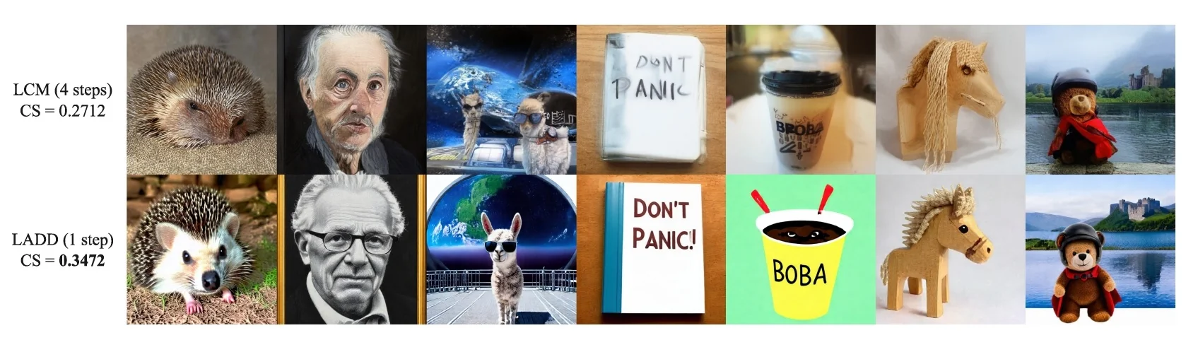
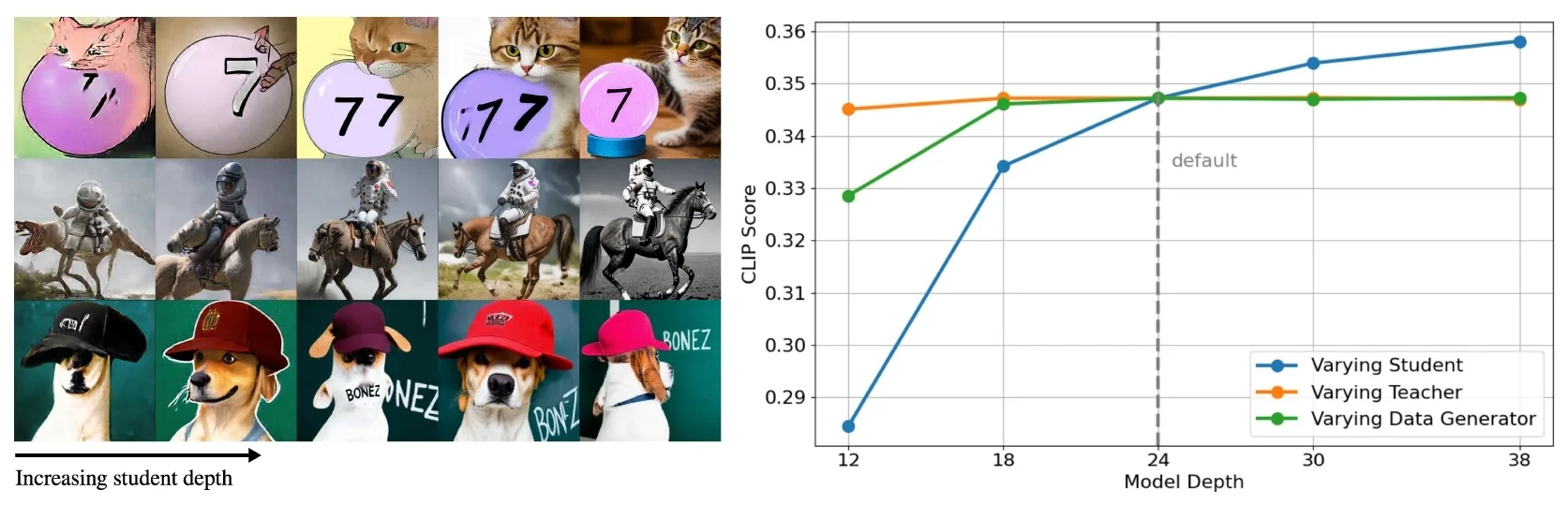
From LADD to SD3-Turbo: Achieving Quality in 1–4 Steps With the pixel-space VAE bottleneck removed, LADD scales naturally to high-resolution, Multi-Aspect Ratio (MAR) training and inference. Sauer et al. instantiate LADD to train SD3-Turbo by distilling Stable Diffusion 3, using an 8B-parameter teacher and a student designed for extremely small step counts [568]. A key practical detail is that SD3-Turbo is trained to produce high-quality samples in unguided sampling, i.e., without classifier-free guidance (CFG) [568]. Empirically, one-step generation is already strong for rapid exploration, but allocating a tiny budget of four unguided steps is sufficient to reach the teacher’s visual quality while improving prompt alignment relative to the one-step setting [568].
Aligning with Human Preference: Diffusion DPO and SD3-Turbo While LADD dramatically accelerates generation and maintains high-frequency realism, adversarial training inherently struggles with structural hallucinations. Because the discriminator heavily evaluates local realism, it can occasionally be fooled by images that possess hyper-realistic textures but absurd global compositions (e.g., a car with three wheels, or an animal with duplicated limbs). To evolve the distilled LADD student into the production-ready SD3-Turbo model, the authors employ a final stage of human preference alignment using Diffusion Direct Preference Optimization (DPO) and Low-Rank Adaptation (LoRA).
What is Diffusion DPO? Diffusion DPO adapts a preference-learning technique originally designed for Large Language Models. Instead of relying purely on a generic text-to-image dataset, DPO trains the model on curated pairs of generated images. Human annotators evaluate outputs for the same prompt, ranking one image as a “win” (structurally sound, aesthetically pleasing, and highly prompt-aligned) and the other as a “loss” (containing adversarial artifacts or hallucinations). The DPO objective mathematically updates the model’s parameters to increase the likelihood of the winning trajectory while penalizing the trajectory of the losing image.
The LoRA Implementation and Transfer Pipeline: Performing DPO on an 8-billion parameter model like Stable Diffusion 3 is computationally prohibitive. Therefore, the authors implement DPO using LoRA. LoRA freezes the massive base model and injects small, trainable low-rank matrices into the transformer’s attention layers. This allows the network to learn a lightweight, modular weight update (\(\Delta W\)) that corrects the artifacts.
The mechanical elegance of the SD3-Turbo pipeline lies in how this single set of preference weights is leveraged across the entire LADD ecosystem. The alignment process unfolds in three strict phases:
- 1.
- Teacher Preference Training: First, DPO is applied to the slow, full-step SD3 teacher. The teacher learns a specific DPO-LoRA (\(\Delta W_{\mbox{DPO}}\)) that successfully suppresses its own characteristic artifacts.
- 2.
- Generating Superior Targets: This DPO-enhanced teacher is then used to generate the synthetic ground truth latents (\(\mathbf {z}_{\mbox{real}}\)) for the LADD training loop. By doing so, the baseline LADD student is trained on a fundamentally cleaner, artifact-free synthetic dataset.
- 3.
- The LoRA Grafting (SD3-Turbo): Once the LADD student has learned the fast 1-to-4 step generation process, it may still exhibit minor adversarial artifacts introduced by the discriminator heads. However, because the student denoiser \(D_\theta \) shares the exact same MMDiT architectural backbone as the teacher, the authors can simply take the \(\Delta W_{\mbox{DPO}}\) learned by the teacher in Step 1 and physically graft it onto the distilled student.
This modular weight transfer is remarkably effective. By reapplying the teacher’s preference LoRA directly to the student, the resulting SD3-Turbo model instantly inherits the human preference alignment. This dramatically reduces adversarial artifacts and improves fine perceptual details without requiring a separate, unstable DPO training phase for the student, and crucially, without altering the student’s ultra-fast 1-to-4 step inference speed [568].
Limitations: The adversarial tightrope remains While LADD resolves the dominant computational bottleneck of pixel-space ADD, it still relies on an adversarial min–max game. In practice, this means training quality depends on careful discriminator-head design, balancing, and stabilization so that the adversarial signal improves realism without destabilizing generation [568]. Moreover, compressing an iterative generative process into 1–4 steps trades away some of the teacher’s controllability: relative to the full teacher, the distilled model shows a modest drop in prompt alignment at very low step counts and offers less flexible control for editing scenarios such as image-to-image or instruction-based editing [568].
Furthermore, the extreme compression of a multi-step stochastic diffusion process into a single forward pass inherently sacrifices some degree of controllability. The distilled student lacks the iterative refinement capacity of its 50-step teacher, resulting in slightly reduced fine-grained prompt adherence and less flexibility in complex compositional reasoning tasks or precise image-to-image editing [568].
Transition: Moving beyond the discriminator LADD answers the engineering question: How can adversarial distillation be made scalable?—by keeping the entire game in latent space and using the teacher as a generative feature lens. This naturally raises a methodological question: Can we remove the min–max discriminator game entirely, while still matching the teacher at the distribution level?
Distribution Matching Distillation (DMD) [759] takes this step. Instead of training a discriminator, DMD formulates one-step distillation as minimizing an approximate KL divergence whose gradient can be written as the difference of two score functions—one for the target (teacher) distribution and one for the current student-induced distribution [759]. This replaces adversarial classification with a discriminator-free distribution-matching signal, aiming for one-step (or few-step) generators without the GAN tightrope.
Enrichment 20.11.20: Distribution Matching Distillation (DMD)
Motivation: Bypassing the GAN Bottleneck ADD and LADD demonstrate that adversarial supervision can compress diffusion sampling into 1–4 steps, but they inherit the classical min–max difficulties of GAN training: stability depends on the capacity and calibration of a discriminator (and careful balancing against the generator), with well-known failure modes such as mode collapse. Distribution Matching Distillation (DMD) [759] removes the discriminator entirely. Instead of learning a real/fake classifier, DMD trains a one-step generator by minimizing a distribution-level divergence between its output distribution and the teacher’s target distribution, using diffusion models themselves as score estimators. This reframes “make it look real” from an adversarial game into a score-based gradient that points toward higher realism and lower fakeness.
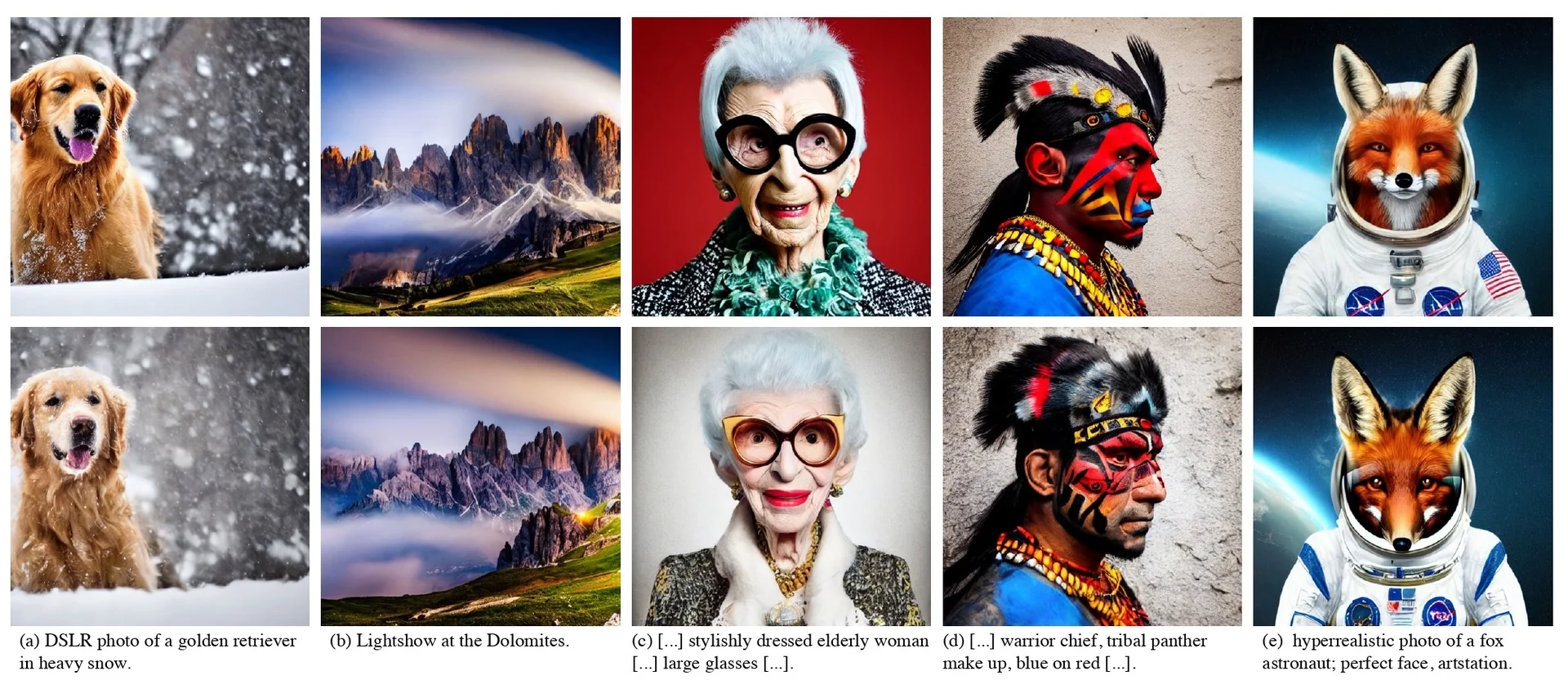
Setup: Three Networks, Two Score Fields, One Generator DMD’s training loop replaces the standard GAN generator-discriminator pair with a triad of neural networks, leveraging score-based gradients to direct optimization:
-
Pretrained base diffusion model \(\mu _{\mbox{base}}\) (real-score estimator): Frozen. This is the original multi-step diffusion denoiser (e.g., Stable Diffusion), rigorously pre-trained on a massive dataset of real images.
Why a multi-step model? Because \(\mu _{\mbox{base}}\) is trained across a dense range of noise levels, it can provide reliable denoising predictions for perturbed inputs \((\mathbf {x}_t,t)\). In diffusion / score-based modeling, such a denoiser can be converted into an estimate of the perturbed real score \(\nabla _{\mathbf {x}_t}\log p_{\mbox{real},t}(\mathbf {x}_t)\), i.e., a vector field defined on the diffused distribution rather than directly on the clean data density.
Intuition: \(\mu _{\mbox{base}}\) acts as a frozen “reality compass” after perturbation: given a noisy image \(\mathbf {x}_t\), it outputs a denoised prediction whose induced score points toward higher-density regions of the \(\mathbf {x}_t\)-space real manifold.
-
One-step generator \(G_\theta \): Trainable. This is the distilled student tasked with mapping a single Gaussian noise draw \(\mathbf {z}\sim \mathcal {N}(\mathbf {0},\mathbf {I})\) directly to an output image \(\mathbf {x}=G_\theta (\mathbf {z})\) in one forward pass.
Architecture & initialization. Following [759], the one-step generator uses the exact denoiser backbone of the pretrained base diffusion model, but operates without dynamic time-conditioning. To preserve tensor shapes and fully reuse the pretrained feature representations without introducing dimension mismatches, the generator’s parameters are initialized directly from the base model (\(\theta \leftarrow \theta _{\mbox{base}}\)). Crucially, “removing time-conditioning” is not achieved by deleting network layers, which would invalidate the pretrained weights. Instead, the timestep input path is permanently locked to the constant maximum-noise embedding (\(T-1\)).
Why specifically \(T-1\) rather than \(T\)? In standard discrete diffusion implementations, the \(T\) total timesteps are zero-indexed from \(0\) (clean data) to \(T-1\) (pure noise). Thus, \(T-1\) is the programmatic ceiling representing a signal-to-noise ratio that is effectively zero; passing an index of \(T\) would result in an out-of-bounds matrix dimension error. Because the generator’s input is pure Gaussian noise \(\mathbf {z}\sim \mathcal {N}(\mathbf {0},\mathbf {I})\), evaluating the base weights at \(T-1\) perfectly aligns the network’s expected input distribution with its actual input. The resulting mapping \(G_\theta :\mathbf {z}\mapsto \mathbf {x}\) becomes a static, single-pass generator that begins training already acting exactly as the teacher would at the very first step of the reverse diffusion process.
Intuition. Even with this powerful initialization, condensing a sequential, fine-grained denoising trajectory into a single massive leap from pure noise to a detailed image is an immensely underconstrained problem. If optimized solely with a perceptual or regression metric (such as LPIPS or \(\ell _2\)), the extreme uncertainty forces the network toward the safest mathematical solution: the conditional expected value. This manifests as severe mode averaging, washing out high-frequency textures and resulting in blurry, oversmoothed images. DMD avoids this regression trap by supervising \(G_\theta \) with a distribution-matching score-field difference. This dual-score gradient explicitly pulls samples toward “more real” regions (injecting high-frequency photorealism) while actively repelling them from the generator’s own collapsing modes (via the fake score model described next), forcing the network to commit to sharp, distinct, and diverse trajectories.
-
Fake diffusion model \(\mu ^{\phi }_{\mbox{fake}}\) (fake-score estimator): Trainable. This is a fully time-conditioned diffusion denoiser, architecturally identical to the base teacher model and initialized with its pre-trained weights. However, instead of being frozen, its parameters \(\phi \) are trained online using a standard diffusion denoising objective applied exclusively to the generator’s continuously evolving fake outputs.
Why a dynamic fake model? The target data manifold is static, meaning the real-score estimator can be permanently frozen. Conversely, the generator’s output distribution (\(p_{\mbox{fake}}\)) is a moving target that shifts at every iteration. To accurately estimate the gradient between the distributions, DMD requires a dynamic critic that constantly maps the shifting topography of what the generator is currently producing.
Intuition (The Repulsive Force): To understand its role, imagine the one-step generator begins to suffer from mode collapse—for instance, mapping many different input noise vectors to the exact same generic, poorly-detailed face. Because the fake denoiser is trained solely on these current outputs, it quickly learns to treat this specific face as a high-density “peak” in the fake distribution.
When a perturbed generated image is passed through this fake denoiser, it calculates the score of the fake distribution: a gradient vector pointing directly uphill toward the center of that concentrated mass. Crucially, the DMD objective updates the generator using the difference \((s_{\mbox{real}} - s_{\mbox{fake}})\). By subtracting the fake score, the gradient mathematically acts as a repulsive force. It actively pushes the generator’s outputs away from their current clumps, aggressively penalizing redundancy. This forces the generator to spread its samples out, preventing mode collapse and ensuring it explores the broader, diverse landscape defined by the real score.
Conceptually, \(\mu _{\mbox{base}}\) defines where the data manifold wants the sample to move (“more real”), while \(\mu ^{\phi }_{\mbox{fake}}\) maps where the generator is currently concentrating its mass (“more fake”). The generator \(G_\theta \) is updated using the difference between these two score directions: it is mathematically pulled toward the modes of reality while being actively repelled from its own centers of mass, simultaneously enforcing photorealism and preventing mode collapse.
Initialization: Reusing the Base Model Without Breaking Shapes A practical concern is how to construct a one-step generator from a time-conditioned denoiser \(\mu _{\mbox{base}}(\mathbf {x}_t,t)\) without invalidating pretrained weights. DMD’s solution is to keep the denoiser backbone but remove the need for a dynamic timestep input at inference.
Concretely, we cannot simply delete the time-embedding layers, as this would cause catastrophic matrix dimension mismatches and destroy the learned pathways. Instead, the one-step generator is initialized from the base model parameters (so it inherits its feature extractors and priors), and its internal timestep path is permanently locked to the maximum-noise embedding (\(T-1\)). Because the generator’s input is pure Gaussian noise \(\mathbf {z}\sim \mathcal {N}(\mathbf {0},\mathbf {I})\), evaluating the base weights at \(T-1\) perfectly aligns the network’s expected input distribution with its actual input. The model is then finetuned as a single-pass map \(G_\theta (\mathbf {z})\) under the distribution matching and regression objectives [759].
Intuition. This is not “training from scratch”: the generator begins with the base model’s rich internal representations, acting exactly as the teacher would at the very first step of the reverse diffusion process. DMD’s score-field gradients provide the missing guidance needed to compress the rest of the iterative denoising trajectory into a single forward pass.
Distribution Matching Objective: Bypassing Intractable Densities via Score Differences Let \(p_{\mbox{fake}}\) be the distribution induced by \(\mathbf {x}=G_\theta (\mathbf {z})\), \(\mathbf {z}\sim \mathcal {N}(\mathbf {0},\mathbf {I})\), and let \(p_{\mbox{real}}\) be the real data distribution (or the teacher’s target distribution). DMD aims to minimize the Kullback-Leibler (KL) divergence between these two distributions: \begin {equation} D_{\mathrm {KL}}\!\big (p_{\mbox{fake}}\;\|\;p_{\mbox{real}}\big ) = \mathbb {E}_{\mathbf {x}\sim p_{\mbox{fake}}} \!\left [ \log \frac {p_{\mbox{fake}}(\mathbf {x})}{p_{\mbox{real}}(\mathbf {x})} \right ]. \label {eq:chapter20_dmd_kl} \end {equation}
The Intractability Problem. In the high-dimensional space of natural images, explicitly evaluating the probability densities \(p_{\mbox{fake}}(\mathbf {x})\) and \(p_{\mbox{real}}(\mathbf {x})\) is computationally intractable. Doing so requires calculating a complex normalization constant (the partition function) by integrating across all possible images. Therefore, directly optimizing Equation 20.136 using density outputs is impossible.
The Score-Based Solution. To bypass this roadblock, we take the gradient of the objective. The gradient of a log-probability yields the score function, \(\nabla _{\mathbf {x}}\log p(\mathbf {x})\). Because the intractable normalization constant is uniform across all \(\mathbf {x}\), its derivative is zero, effectively dropping out of the equation entirely.
Thus, the gradient of the KL divergence with respect to the generator’s parameters \(\theta \) can be elegantly rewritten strictly using score fields: \(s_{\mbox{real}}(\mathbf {x})=\nabla _{\mathbf {x}}\log p_{\mbox{real}}(\mathbf {x})\) and \(s_{\mbox{fake}}(\mathbf {x})=\nabla _{\mathbf {x}}\log p_{\mbox{fake}}(\mathbf {x})\): \begin {equation} \nabla _\theta D_{\mathrm {KL}} = \mathbb {E}_{\mathbf {z}} \!\left [ -\big (s_{\mbox{real}}(\mathbf {x})-s_{\mbox{fake}}(\mathbf {x})\big )\, \frac {dG_\theta (\mathbf {z})}{d\theta } \right ], \qquad \mathbf {x}=G_\theta (\mathbf {z}). \label {eq:chapter20_dmd_grad_clean} \end {equation}
Intuition: This formulation brilliantly reframes density matching as a vector-field matching problem. The term \(s_{\mbox{real}}(\mathbf {x})\) acts as an attractive force, pulling the generated samples uphill toward the high-density peaks of reality. Conversely, \(-s_{\mbox{fake}}(\mathbf {x})\) acts as a repulsive force, spreading samples away from the generator is currently collapsing its mass, preventing mode collapse and explicitly enforcing output diversity.
Why Perturbation is Necessary: Making the Objective Well-Defined Evaluating the score-difference form of Eq. (20.137) directly on clean samples \(\mathbf {x}=G_\theta (\mathbf {z})\) is generally ill-posed in high dimensions: the supports of \(p_{\mbox{real}}\) and \(p_{\mbox{fake}}\) can be effectively disjoint, so a meaningful “direction from fake to real” may not exist everywhere. DMD resolves this by applying a forward diffusion perturbation, which smooths both distributions and makes them overlap in \(\mathbf {x}_t\)-space, so the distribution-matching objective becomes well-defined.
A second (practical) reason is numerical: as the noise level becomes extremely small (\(\sigma _t\to 0\)), score estimates and their induced gradients become unstable. Accordingly, DMD samples timesteps from a bounded interval \([T_{\min },T_{\max }]\) (implemented as a restricted timestep range) rather than using arbitrarily tiny noise levels:
\begin {equation} q_t(\mathbf {x}_t\mid \mathbf {x}) = \mathcal {N}\!\big (\alpha _t \mathbf {x},\,\sigma _t^2\mathbf {I}\big ), \qquad \mathbf {x}_t\sim q_t(\mathbf {x}_t\mid \mathbf {x}). \label {eq:chapter20_dmd_perturbation} \end {equation}
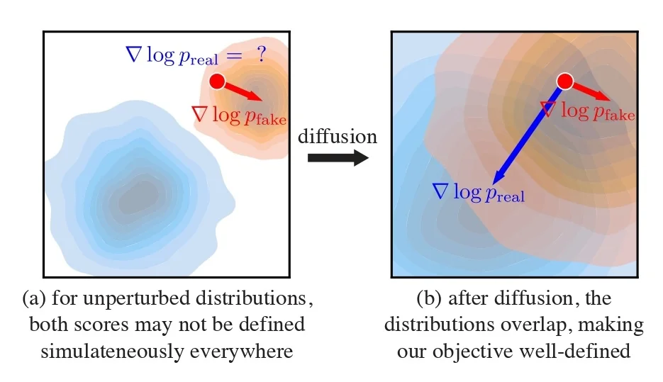
Estimating the Real and Fake Scores with Two Diffusion Models After perturbation, DMD estimates score functions on the diffused distributions using diffusion denoisers. For clarity, we present the common mean-prediction form used in [759]: if a denoiser \(\mu (\mathbf {x}_t,t)\) predicts the conditional mean / denoised estimate, then the induced score on the Gaussian corruption kernel admits the closed form \begin {equation} s(\mathbf {x}_t,t) = \nabla _{\mathbf {x}_t}\log p(\mathbf {x}_t) = - \frac {\mathbf {x}_t-\alpha _t\,\mu (\mathbf {x}_t,t)}{\sigma _t^2}. \label {eq:chapter20_dmd_score_from_mu} \end {equation} Note: Other parameterizations such as \(\epsilon \)-prediction can be converted to an equivalent denoised estimate and plugged into the same template; [759] uses mean prediction for simplicity.
Using Eq. (20.139), DMD defines: \begin {align} s_{\text {real}}(\mathbf {x}_t,t) &= - \frac {\mathbf {x}_t-\alpha _t\,\mu _{\text {base}}(\mathbf {x}_t,t)}{\sigma _t^2}, \label {eq:chapter20_dmd_s_real} \\ s_{\text {fake}}(\mathbf {x}_t,t) &= - \frac {\mathbf {x}_t-\alpha _t\,\mu ^{\phi }_{\text {fake}}(\mathbf {x}_t,t)}{\sigma _t^2}. \label {eq:chapter20_dmd_s_fake} \end {align}
Training the Fake Score Estimator (The Online Critic) To ensure \(s_{\mbox{fake}}\) accurately maps the generator’s shifting topography, the fake denoiser \(\mu ^{\phi }_{\mbox{fake}}\) must be trained simultaneously. It is updated using the standard diffusion denoising objective, explicitly restricted to only see the generator’s outputs. To prevent the critic from altering the generator during its own update, gradients are stopped at the generator’s boundary:
\begin {equation} \mathcal {L}^{\phi }_{\mbox{denoise}} = \big \| \mu ^{\phi }_{\mbox{fake}}(\mathbf {x}_t,t) - \operatorname {stopgrad}(\mathbf {x}) \big \|_2^2, \label {eq:chapter20_dmd_fake_loss} \end {equation}
where \(\mathbf {x}=G_\theta (\mathbf {z})\) and \(\mathbf {x}_t\sim q_t(\mathbf {x}_t\mid \operatorname {stopgrad}(\mathbf {x}))\).
The Distribution Matching Gradient and Sample Weighting Replacing the intractable clean-image scores in Eq. (20.137) with the perturbed score estimators yields the practical DMD update direction. However, directly applying this raw difference introduces a severe optimization hazard: the scale imbalance across noise levels.
In diffusion models, the raw numerical magnitude of the score difference \(\big (s_{\mbox{fake}}(\mathbf {x}_t,t)-s_{\mbox{real}}(\mathbf {x}_t,t)\big )\) fluctuates drastically depending on the timestep \(t\). If these unscaled gradients are backpropagated directly, timesteps with naturally larger numerical scales will violently dominate the optimization process, causing training instability and preventing the generator from learning fine details.
To counteract this, DMD introduces an adaptive, time-dependent weight \(w(t)\) to dynamically normalize the gradient magnitude. Following [759], \(w(t)\) is computed as the inverse of the mean absolute deviation (L1 distance) between the generator’s clean output \(\mathbf {x}\) and the base model’s denoised prediction \(\mu _{\mbox{base}}\) at that specific noise level:
\begin {equation} w(t) = \frac {1}{\mathrm {mean}\!\left (\left |\mathbf {x}-\mu _{\mbox{base}}(\mathbf {x}_t,t)\right |\right )}, \qquad \mathbf {x}=G_\theta (\mathbf {z}). \label {eq:chapter20_dmd_wt} \end {equation}
The Idea and Stabilization Intuition: What does this weight actually do? By multiplying the update by \(w(t)\), we are effectively dividing the gradient by its expected spatial magnitude at that exact timestep. This auto-normalizes the training signal so that the gradient step size is roughly uniform across all \(t\). It guarantees that the generator pays equal attention to high-noise timesteps (which correct global, macroscopic structure) and low-noise timesteps (which refine high-frequency, local textures), rather than letting one noise regime arbitrarily overpower the other.
Putting this together, the generator receives the scale-normalized approximate KL gradient (up to standard Jacobian factors) in the form:
\begin {equation} \nabla _\theta D_{\mathrm {KL}} \simeq \mathbb {E}_{\mathbf {z},t,\mathbf {x}_t} \!\left [ w(t)\, \big (s_{\mbox{fake}}(\mathbf {x}_t,t)-s_{\mbox{real}}(\mathbf {x}_t,t)\big )\, \frac {dG_\theta (\mathbf {z})}{d\theta } \right ]. \label {eq:chapter20_dmd_final_grad} \end {equation}
Implementation note: To further avoid boundary instabilities (where the score functions become mathematically undefined at exactly \(t=0\) or \(t=T\)), the timestep \(t\) is sampled over a strictly bounded interval \([T_{\min },T_{\max }]\) (e.g., \(0.02T\) to \(0.98T\)) as prescribed in [759]. The mean absolute deviation in Equation 20.141 is averaged over all spatial and channel dimensions of the sample, yielding a highly stable, scalar-normalized gradient signal ready for the optimizer.
Regression Loss: A Structural Anchor that Prevents Mode Dropping While the KL gradient successfully forces the generated images to look photorealistic, relying solely on distribution matching leaves the generator highly susceptible to catastrophic mode dropping. To understand why, we must look at the mathematical asymmetry of the reverse-KL divergence objective:
\begin {equation} D_{\mathrm {KL}}\!\big (p_{\mbox{fake}}\;\|\;p_{\mbox{real}}\big ) = \mathbb {E}_{\mathbf {x}\sim p_{\mbox{fake}}} \!\left [ \log \frac {p_{\mbox{fake}}(\mathbf {x})}{p_{\mbox{real}}(\mathbf {x})} \right ]. \end {equation}
Because the expectation is evaluated over the generator’s distribution (\(p_{\mbox{fake}}\)), the penalty is heavily one-sided. If the generator produces an unrealistic image (placing mass where \(p_{\mbox{real}}\) is near zero), the ratio explodes, incurring a massive penalty. Thus, the generator is fiercely penalized for generating ”fake-looking” images. However, if the generator simply ignores an entire valid mode of the real data manifold (i.e., \(p_{\mbox{real}}\) is high, but \(p_{\mbox{fake}}\) is zero), that region contributes exactly zero to the expected loss.
Consequently, reverse-KL is inherently mode-seeking. The safest optimization path for the generator is to find a small handful of highly realistic modes and collapse all its random noise inputs into them, completely ignoring the rich diversity of the full data manifold.
To firmly anchor the one-step generator’s large-scale structure and explicitly enforce diversity, DMD integrates an offline regression loss. The authors pre-compute a modest dataset \(\mathcal {D}=\{(\mathbf {z},\mathbf {y})\}\) by running the slow, multi-step teacher ODE solver from initial noise \(\mathbf {z}\) to a final high-quality image \(\mathbf {y}\). DMD enforces a Learned Perceptual Image Patch Similarity (LPIPS) penalty between the one-step output and this multi-step target:
\begin {equation} \mathcal {L}_{\mbox{reg}} = \mathbb {E}_{(\mathbf {z},\mathbf {y})\sim \mathcal {D}} \Big [ \mbox{LPIPS}\!\big (G_\theta (\mathbf {z}),\,\mathbf {y}\big ) \Big ]. \label {eq:chapter20_dmd_reg_loss} \end {equation}
The total objective optimized by the one-step generator \(G_\theta \) is the combination of the distribution matching step and the regression step:
\begin {equation} \begin {split} \min _\theta \;\; & D_{\mathrm {KL}} \;+\; \lambda _{\mbox{reg}}\mathcal {L}_{\mbox{reg}}, \\ \mbox{where} \quad \lambda _{\mbox{reg}} &= \begin {cases} 0.25 & \mbox{(class-conditional and SDv1.5 default)}, \\ 0.5 & \mbox{(unconditional setting)}. \end {cases} \end {split} \label {eq:chapter20_dmd_total_loss} \end {equation}
Intuition: Why does regression solve mode collapse? The offline dataset \(\mathcal {D}\) represents the full, diverse span of the teacher’s capabilities. It explicitly pairs every unique noise vector \(\mathbf {z}\) to a distinctly different target image \(\mathbf {y}\). If the generator attempts to collapse multiple \(\mathbf {z}\) inputs into a single ”safe” mode to satisfy the KL loss, the LPIPS distance penalty for most of those pairs will skyrocket.
Thus, the regression loss acts as a “compositional leash”. It physically forces the one-step generator’s mapping to maintain the topological spread and global layout of the teacher’s manifold. It guarantees diversity, while the distribution-matching gradient operates on top of this anchored structure to inject the high-frequency photorealism that a pure regression loss would blur away.
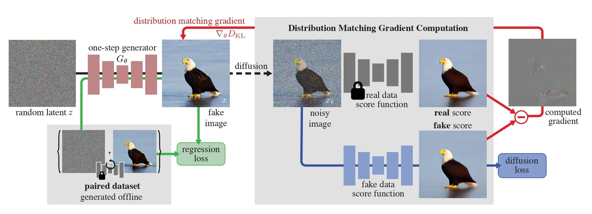
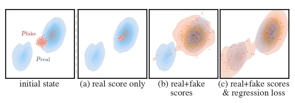
Training Loop: Two Tracks, No Multi-Step Sampling With the total objective fully defined, each training iteration simply alternates between two parallel updates:
- Update the Generator (\(G_\theta \)): Sample fresh noise \(\mathbf {z}\) to compute the distribution matching gradient \(\nabla _\theta D_{\mathrm {KL}}\) (using the score difference on perturbed samples), and sample a paired \((\mathbf {z},\mathbf {y})\) from the offline dataset to compute the regression gradient \(\nabla _\theta \mathcal {L}_{\mbox{reg}}\). Apply the combined gradient \(\nabla _\theta (D_{\mathrm {KL}} + \lambda _{\mbox{reg}}\mathcal {L}_{\mbox{reg}})\) to update \(\theta \).
- Update the Fake Score Estimator (\(\mu ^{\phi }_{\mbox{fake}}\)): Sample fake images \(\mathbf {x}=G_\theta (\mathbf {z})\), apply a stop-gradient, perturb them to \(\mathbf {x}_t\), and update the critic’s parameters \(\phi \) using the standard diffusion denoising loss.
Crucially, the computationally expensive multi-step teacher sampler is never run iteratively inside the online training loop. The massive frozen base model is used strictly as a single-forward-pass score estimator on \((\mathbf {x}_t,t)\). All multi-step sequential sampling is entirely relegated to the offline dataset construction.
Experiments and Ablations: What Matters in Practice DMD demonstrates remarkable one-step generation capabilities across both class-conditional benchmarks (e.g., achieving an FID of 2.62 on ImageNet \(64\times 64\)) and complex text-to-image distillation tasks (e.g., Stable Diffusion on MS-COCO). It closes the vast majority of the fidelity gap to its multi-step teachers while slashing inference latency by factors of 30\(\times \) to 100\(\times \) (e.g., reducing generation time from 2590ms to 90ms) [759].
Ablations explicitly confirm the necessity of the tri-network design (as visualized previously in Figure 20.179):
- Distribution matching is strictly required for photorealism. Relying on regression alone causes the model to regress to blurry, expected-value textures, entirely missing the sharp target distributions.
- Regression anchoring is strictly required to prevent mode dropping. Without it, the model achieves local realism but suffers catastrophic mode collapse, failing to preserve the teacher’s compositional diversity.
- Timestep weighting (\(w_t\)) is essential to stabilize training across the extreme variance in gradient magnitudes between low-noise and high-noise timesteps.
Transition: From Adversarial Games to Score-Field Games LADD demonstrated how to make adversarial distillation computationally viable by moving the discriminator into latent space. DMD pushes this philosophy to its logical extreme by removing the discriminator entirely. By replacing binary real/fake classification with a continuous score-field difference, DMD directly optimizes a theoretically grounded distribution-level objective.
This establishes a unifying perspective for modern fast samplers: ultra-fast generators can be successfully supervised either by learned adversarial discriminators (ADD/LADD) or by learned score fields that mathematically define the exact vector flows between distributions (DMD). This elegant reframing sets the stage for exploring flow-based formulations and continuous trajectory matching in subsequent chapters.
Enrichment 20.11.21: D3PM: Structured Diffusion in Discrete Spaces
Motivation: The Discrete Data Bottleneck Standard Denoising Diffusion Probabilistic Models (DDPMs) rely on additive Gaussian noise, a formulation uniquely suited for continuous, real-valued manifolds. However, this assumption is fundamentally incompatible with inherently discrete or categorical data, such as text tokens, semantic segmentation labels, or heavily quantized image pixels. Early attempts to adapt diffusion to discrete spaces applied a naïve uniform corruption—where a token transitions to a uniformly random vocabulary item (including possibly staying the same) with equal probability. This unstructured approach destroys critical domain knowledge; for example, it ignores the ordinal relationship of pixel intensities or the semantic proximity of words. Discrete Denoising Diffusion Probabilistic Models (D3PM) [18] resolve this limitation by generalizing the forward corruption process, replacing additive Gaussian noise with a structured Markov chain governed by domain-specific transition matrices.
Intuition: Corruption as a Structural Prior In continuous diffusion, adding Gaussian noise acts like a gradual, structured blur. However, applying continuous math to discrete structures introduces fundamental mismatches—such as relaxing categorical/quantized states to continuous values for corruption and then quantizing at the end, which imposes an arbitrary continuous geometry on a discrete space. D3PM replaces additive noise with Markov transition probabilities, strictly maintaining the discrete nature of the data throughout the entire process.
By custom-designing the transition matrix \(Q_t\), we dictate exactly how the data degrades, creating a powerful structural prior for the reverse generative process. The authors propose four distinct matrix families to address different data modalities [18]:
- Absorbing State (Masking for Text): Instead of corrupting a valid token into an arbitrary incorrect token, the transition matrix moves it into a dedicated absorbing [MASK] state from which it cannot escape. The forward chain therefore converges to a point mass on [MASK], and generation becomes iterative “unmasking” in reverse—a discrete diffusion view that cleanly connects to masked modeling objectives [18].
- Discretized Gaussian (Ordinality for Quantized Images): For ordinal discrete values (e.g., per-channel 8-bit pixel intensities), D3PM uses a discretized, truncated Gaussian-like kernel: states closer in index receive higher transition probability, and large jumps become exponentially unlikely (but are generally not forbidden). Concretely, for \(i\neq j\) the off-diagonal mass is proportional to \( \exp \!\big (-4|i-j|^2/((K-1)^2\beta _t)\big ) \) and is normalized over a truncated index range; the diagonal entry is then set to the remaining probability mass so that each row sums to one. With this normalization, the resulting \(Q_t\) is irreducible and doubly stochastic, hence it has a uniform stationary distribution while still injecting an ordinal locality bias in intermediate corruption steps.
-
Token embedding distance (semantic locality): D3PM can define “local” corruption in text via a \(k\)-nearest-neighbor graph in a pretrained embedding space. The construction symmetrizes the graph, builds a (row-sum-zero) rate matrix \(R\), and defines \(Q_t = \exp (\alpha _t R)\).
Since \(R\) is symmetric and sums to zero along each row, \(Q_t=\exp (\alpha _t R)\) is doubly stochastic. This ensures a uniform stationary distribution (in particular, when the underlying \(k\)-NN graph is connected, the chain mixes to that uniform limit), while biasing intermediate transitions toward embedding-near substitutions.
Empirically, however, this “nearest-neighbor diffusion” can be a cautionary negative result on LM1B: embedding similarity is not necessarily the right notion of locality for a diffusion process in language.
-
Uniform (Uninformative baseline for unordered categories): For genuinely unordered labels (e.g., categorical semantic segmentation classes like “Car,” “Tree,” or “Sky”), there is no meaningful notion of “small” vs. “large” perturbations.
In such cases, imposing an ordinal metric or semantic distance is semantically unjustified. A standard “no structure assumed” corruption is uniform diffusion: with probability \(1-\beta _t\) we keep the token unchanged, and with probability \(\beta _t\) we resample uniformly from the \(K\) categories. Equivalently, \( Q_t = (1-\beta _t)I + \frac {\beta _t}{K}\mathbf {1}\mathbf {1}^\top , \) which is doubly stochastic and has a uniform stationary distribution.
D3PM’s uniform matrix therefore serves as the principled “no structure assumed” baseline, preserving a well-defined Markov forward process and a uniform stationary distribution [18].
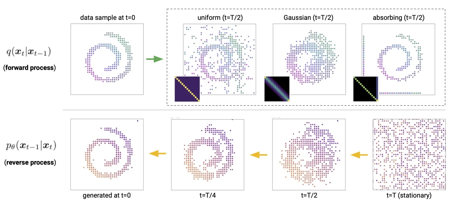
Setup: The Forward Process as a Discrete Markov Chain Instead of adding continuous Gaussian noise, D3PM corrupts a discrete random variable over \(T\) timesteps using a time-inhomogeneous Markov chain. Let \(x_t\) be a scalar discrete variable with \(K\) possible categories (e.g., the size of a token vocabulary, or \(K=256\) for 8-bit pixel intensity bins). Following [18], we represent \(x_t\) as a one-hot row vector of length \(K\).
The transition probabilities from time \(t-1\) to \(t\) are defined by a state transition matrix \(Q_t \in \mathbb {R}^{K \times K}\), where each entry specifies the probability of a token corrupting from state \(i\) to state \(j\): \[ [Q_t]_{ij} \;=\; q(x_t{=}j \mid x_{t-1}{=}i). \] Because \(Q_t\) is a valid transition matrix, each row must sum to one to conserve probability mass (\(\sum _{j=1}^K [Q_t]_{ij}=1\)). The forward corruption step for a single token can thus be elegantly written as a categorical distribution parameterized by a row-vector-matrix product:
\begin {equation} q(x_t \mid x_{t-1}) = \mathrm {Cat}\!\Big (x_t;\; p = x_{t-1} Q_t\Big ). \label {eq:chapter20_d3pm_forward_step} \end {equation}
Factorization over dimensions (Scaling to Images and Text). In practice, our actual data \(\mathbf {x}_t\) is high-dimensional. For example, a single \(32 \times 32\) RGB image contains \(N = 32 \times 32 \times 3 = 3072\) separate discrete variables (pixels).
D3PM makes a crucial simplifying assumption: the corruption process is applied to each coordinate (each pixel or text token) entirely independently. This means the full joint distribution of the image factorizes perfectly across all spatial or sequence positions:
\begin {equation} q(\mathbf {x}_t \mid \mathbf {x}_{t-1}) = \prod _{n=1}^N q(x_t^{(n)} \mid x_{t-1}^{(n)}). \label {eq:chapter20_d3pm_factorization} \end {equation}
Concurrent and Batched Computation. If the process is applied per-pixel, does this mean we must simulate the corruption using a slow, sequential for loop over all \(N\) pixels? Fortunately, no.
Because the corruption is conditionally independent and utilizes the exact same transition matrix \(Q_t\) for every single coordinate, we can compute the entire forward step concurrently using highly optimized tensor operations. By reshaping our entire clean image \(\mathbf {x}_{t-1}\) into a flattened matrix \(\mathbf {X}_{t-1}\) of shape \(N \times K\) (where each row is a one-hot vector), we can find the transition probabilities for the entire image via a single dense matrix multiplication:
\begin {equation} \mathbf {P} = \mathbf {X}_{t-1} Q_t. \label {eq:chapter20_d3pm_tensorized_step} \end {equation}
The result, \(\mathbf {P}\), is an \(N \times K\) matrix containing the exact categorical probability distributions for every single pixel simultaneously. We then sample the entire noisy image \(\mathbf {X}_t\) concurrently across the \(N\) dimension.
This matrix formulation trivially extends to deep learning batching (yielding a \(B \times N \times K\) tensor). This perfectly leverages GPU parallelization, allowing the core mathematical framework of D3PM to be derived strictly for a single coordinate \(x_t\) while scaling computationally efficiently to high-dimensional datasets.
Closed-form marginals (The Discrete Jump). In continuous DDPMs, a key property is the ability to sample the noisy state \(\mathbf {x}_t\) directly from the clean data \(\mathbf {x}_0\) without iteratively simulating the entire forward chain step-by-step. D3PM mathematically preserves this critical property for discrete spaces. Because Markov chains possess the property of associative matrix multiplication over time, the cumulative transition probability from the clean data \(x_0\) to any arbitrary timestep \(t\) is simply the product of the intermediate matrices:
\begin {equation} \overline {Q}_t \;=\; Q_1 Q_2 \cdots Q_t. \label {eq:chapter20_d3pm_Qbar} \end {equation}
Consequently, the \(t\)-step marginal distribution is given in closed form:
\begin {equation} q(x_t \mid x_0) = \mathrm {Cat}\!\Big (x_t;\; p = x_0\,\overline {Q}_t\Big ). \label {eq:chapter20_d3pm_forward_marginal} \end {equation}
This closed-form marginal is the engine of practical deep learning training. During training, we do not need to slowly corrupt an image 1,000 times to get the target for step \(t=1000\). Instead, we randomly sample a timestep \(t \sim \mathcal {U}(1, T)\), precompute \(\overline {Q}_t\), instantly jump to the corrupted state \(x_t\), and compute the loss. This entirely bypasses the need for sequential simulation loops during the forward pass.
Designing \(Q_t\): Stationary limits as the notion of “full corruption” A central design choice in D3PM is the stationary distribution of the forward Markov chain, i.e., what \(x_t\) converges to as \(t\) becomes large. For uniform diffusion, the paper uses the classical categorical transition \( Q_t = (1-\beta _t)I + \frac {\beta _t}{K}\mathbf {1}\mathbf {1}^\top , \) which is doubly stochastic and therefore has a uniform stationary distribution over the \(K\) categories. The discretized-Gaussian and token-embedding constructions are also designed to be (approximately) doubly stochastic, so they share the same uniform stationary limit, but inject different notions of locality into the intermediate corruption steps. In contrast, absorbing-state diffusion deliberately chooses a different stationary limit: all probability mass concentrates on the absorbing token (e.g., [MASK]), yielding a BERT-like “generate by iterative unmasking” process.
Method: Enforcing Structure in the Reverse Process In continuous diffusion, the neural network typically predicts the added continuous noise (from which the previous state \(\mathbf {x}_{t-1}\) is derived). In discrete spaces, the most intuitive equivalent would be to have the network directly predict the categorical distribution for the previous step: \(p_\theta (x_{t-1} \mid x_t)\).
However, directly predicting logits for \(p_\theta (x_{t-1}\mid x_t)\) leaves the reverse kernel unconstrained: it may ignore (or fight against) the inductive bias encoded by the chosen forward transition \(Q_t\). D3PM therefore adopts the \(x_0\)-parameterization: the network predicts a distribution over the clean state, \(\tilde {p}_\theta (\tilde {x}_0\mid x_t)\), and the reverse transition is obtained by composing this prediction with the exact forward-process posterior. This construction has two key effects. First, whenever the forward likelihood \(q(x_t\mid x_{t-1})\) has hard zeros (e.g., absorbing-state diffusion, or explicitly band-limited kernels), the reverse transition can only place mass on states that are reachable under the forward process, inheriting its support constraints. Second, even when \(Q_t\) is dense (e.g., discretized-Gaussian or matrix-exponential constructions), the reverse kernel is still forced to respect the relative transition geometry encoded by \(Q_t\), because it is built by reweighting exact posteriors rather than being learned as an arbitrary categorical map.
We can break this mechanism down into three distinct phases: the mathematical foundation of the forward process, the neural network’s role, and the actual inference step.
Phase 1: The Forward Process and the Exact Posterior
During the forward corruption process, we systematically destroy data using our
custom-designed matrices \(Q_t\). Crucially, this forward pass is inherently stochastic,
not deterministic. For a given token \(x_{t-1}\), the corresponding row in \(Q_t\) provides a
probability distribution over all possible \(K\) categories for the next timestep. We do
not simply select the category with the maximal probability; rather, we
randomly draw the next state according to those exact probabilities: \(x_t \sim \mathrm {Cat}(x_{t-1}Q_t)\).
This random sampling is what injects stochastic noise into the discrete
system.
Because we explicitly defined the mathematical rules governing this stochastic forward chain, if we magically knew the true, clean starting data \(x_0\), the distribution of the previous step \(x_{t-1}\) given our current noisy state \(x_t\) is not something the network needs to guess—it is an exact mathematical certainty governed by Bayes’ rule.
Using the Markov property, this forward posterior is given in closed form:
\begin {equation} q(x_{t-1} \mid x_t, x_0) = \frac {q(x_t \mid x_{t-1}, x_0) q(x_{t-1} \mid x_0)}{q(x_t \mid x_0)} = \frac {q(x_t \mid x_{t-1}) q(x_{t-1} \mid x_0)}{q(x_t \mid x_0)}. \label {eq:chapter20_d3pm_bayes} \end {equation}
Substituting our known categorical matrix formulations into this ratio yields a computable, closed-form equation:
\begin {equation} q(x_{t-1} \mid x_t, x_0) = \mathrm {Cat}\!\left ( x_{t-1};\; p = \frac { \big (x_t Q_t^\top \big )\;\odot \;\big (x_0 \overline {Q}_{t-1}\big ) }{ x_0 \overline {Q}_t x_t^\top } \right ). \label {eq:chapter20_d3pm_posterior} \end {equation}
Intuition for Eq. 20.152: The numerator is the element-wise product (\(\odot \)) of two pathways: the probability of transitioning from any candidate \(x_{t-1}\) into our current known \(x_t\), multiplied by the probability of reaching that candidate \(x_{t-1}\) from the clean \(x_0\). The denominator (\(x_0 \overline {Q}_t x_t^\top \in \mathbb {R}\)) is simply the scalar normalization constant representing the total probability of going directly from \(x_0\) to \(x_t\).
Phase 2: The Backward Process (Predict \(x_0\) and Marginalize)
In reality, during the reverse generation process, we do not have access to
the clean data \(x_0\). If we trained a neural network to directly predict \(p_\theta (x_{t-1}\mid x_t)\), it
could ignore the inductive bias encoded by \(Q_t\), and—when \(q(x_t\mid x_{t-1})\) contains hard
zeros—assign nonzero mass to transitions that the forward process deems
impossible.
To solve this, D3PM tasks the neural network with a different goal: take the current noisy state \(x_t\) and output a categorical distribution representing its best guess of the original clean data, denoted as \(\tilde {p}_\theta (\tilde {x}_0 \mid x_t)\).
Once the network provides this distribution over all possible clean states, we mathematically derive the reverse step using the Law of Total Probability. We can break this derivation down step-by-step:
- 1.
- Step 1: Factorizing the Reverse Step via the Chain Rule
Our ultimate goal is to model the reverse transition \(p_\theta (x_{t-1} \mid x_t)\). To inject the structural rules of the forward process into this prediction, we introduce the uncorrupted clean data \(x_0\) as a latent “middleman”.Using the Law of Total Probability and the chain rule of probability, we can expand our target distribution by summing over all \(K\) possible categories for the hypothetical clean state, which we denote as \(\tilde {x}_0\):
\begin {align} p_\theta (x_{t-1} \mid x_t) &= \sum _{\tilde {x}_0=1}^K p_\theta (x_{t-1}, \tilde {x}_0 \mid x_t) \nonumber \\ &= \sum _{\tilde {x}_0=1}^K \underbrace {p_\theta (x_{t-1} \mid x_t, \tilde {x}_0)}_{\text {Reverse step if we knew } x_0} \;\times \; \underbrace {p_\theta (\tilde {x}_0 \mid x_t)}_{\text {Guess of } x_0}. \label {eq:chapter20_d3pm_chain_rule} \end {align}
This factorization elegantly splits the problem into two distinct parts: guessing the clean data, and stepping backward conditionally.
- 2.
- Step 2: The Network’s Job (Predicting the Clean State)
Look at the right-most term in Equation [ref]: \(p_\theta (\tilde {x}_0 \mid x_t)\). This asks, “Given the current noisy data \(x_t\), what is the probability that the original clean data was \(\tilde {x}_0\)?” This is exactly what our deep neural network will model.The network takes \(x_t\), processes it, and outputs a \(K\)-dimensional softmax distribution (e.g., logits over the entire vocabulary or pixel color palette) representing its confidence in every possible original state. We denote the network’s output as \(\tilde {p}_\theta (\tilde {x}_0 \mid x_t)\).
- 3.
- Step 3: The Structural Bottleneck (Substitution)
Now look at the left term: \(p_\theta (x_{t-1} \mid x_t, \tilde {x}_0)\). This asks, “If we knew the current state was \(x_t\) and we assumed the clean state was \(\tilde {x}_0\), what is the probability of the previous state being \(x_{t-1}\)?”Here lies the brilliance of D3PM: we do not need to use machine learning for this. If we assume a specific clean state \(\tilde {x}_0\) is the absolute truth, the path backward is strictly dictated by the rules of probability we established during the forward corruption process. It is exactly the mathematical forward posterior \(q(x_{t-1} \mid x_t, \tilde {x}_0)\) that we derived in Phase 1 (Equation 20.152).
Therefore, D3PM forcefully anchors the reverse process to reality by making a strict substitution: we replace the trainable parameter \(p_\theta (x_{t-1} \mid x_t, \tilde {x}_0)\) with the exact, unchangeable mathematical ground truth \(q(x_{t-1} \mid x_t, \tilde {x}_0)\).
- 4.
- Step 4: The Final Marginalization (The Weighted Average)
Substituting our neural network and our exact posterior back into our original factorization (Equation [ref]), we arrive at the final formulation for the reverse step: \begin {equation} p_\theta (x_{t-1} \mid x_t) = \sum _{\tilde {x}_0=1}^K \underbrace {q(x_{t-1} \mid x_t, \tilde {x}_0)}_{\mbox{Exact mathematical rulebook}} \;\times \; \underbrace {\tilde {p}_\theta (\tilde {x}_0 \mid x_t)}_{\mbox{Neural network's confidence}}. \label {eq:chapter20_d3pm_reverse_step} \end {equation}
Intuition (The Weighted Vote in Categorical Space): Think of Equation 20.153 as a weighted voting system operating on probability vectors. To understand the mechanics, let’s track the shapes and operations for a single token (e.g., a single pixel with \(K=256\) possible color intensities, where a specific state is represented as a \(1 \times K\) one-hot vector).
- The Network’s Output (\(\tilde {p}_\theta \)): The neural network observes the corrupted state \(x_t\) and outputs a dense vector of shape \(1 \times K\) containing probability scores that sum to 1. This vector represents the network’s confidence across all \(K\) candidates for what the original pixel (\(\tilde {x}_0\)) was. For example, it might assign a probability of 0.8 to the “Bright Red” category, 0.2 to the “Dark Red” category, and exactly 0.0 to the other 254 colors.
- The Mathematical Rulebook (\(q\)): For every single one of those \(K\) candidates, we consult the exact forward posterior \(q(x_{t-1} \mid x_t, \tilde {x}_0)\). As derived in Phase 1, this formula takes the current noisy state \(x_t\) and the hypothetical clean state \(\tilde {x}_0\), and evaluates the rigid rules of the forward matrix \(Q_t\). For any given candidate, this rulebook outputs a \(1 \times K\) probability vector specifying exactly what the previous step \(x_{t-1}\) must be. For instance, if the candidate was Bright Red, the rulebook outputs a \(1 \times K\) vector (let’s call it Distribution A). If the candidate was Dark Red, it outputs a different \(1 \times K\) vector (Distribution B).
- The Final Step (Marginalization): The final reverse step \(p_\theta (x_{t-1} \mid x_t)\) is simply the weighted sum of these vectors. We multiply Distribution A by the scalar 0.8, multiply Distribution B by the scalar 0.2, and add them together. The result is our final \(1 \times K\) categorical distribution for sampling the next token.
Key Payoff: The Reverse Kernel Inherits the Forward Geometry (and Support When Present). Why not let the network output \(p_\theta (x_{t-1}\mid x_t)\) directly?
-
Hard Constraints (True Zeros): According to the posterior decomposition, the optimal reverse transition from a given \(x_t\) only considers predecessors \(x_{t-1}\) for which \(q(x_t\mid x_{t-1})\) is non-zero. Thus, when \(Q_t\) encodes true zeros (e.g., absorbing-state diffusion, or explicitly band-diagonal kernels), the ideal reverse kernel is sparse in exactly the same locations.
The \(x_0\)-parameterization inherits this sparsity automatically, because \(p_\theta (x_{t-1}\mid x_t)\) is built by marginalizing exact posteriors whose support is dictated by \(Q_t\).
- If \(Q_t\) is dense (no hard zeros): For discretized-Gaussian and matrix-exponential constructions, large moves are typically suppressed rather than forbidden. In this common case, the advantage is not “hard validity,” but consistency: the learned reverse kernel is tied to the exact Bayesian posterior of the chosen forward process, ensuring the model’s denoising steps reflect the same transition geometry and stationary limit designed into \(Q_t\).
Phase 3: Inference (Generation)
Once the neural network \(\tilde {p}_\theta \) is fully trained, we can discard the forward
corruption process entirely. To generate a completely new data sample
from scratch, we simulate the reverse Markov chain starting from pure
noise.
- 1.
- Initialization (\(t=T\)): We begin by sampling an initial state \(x_T\) from the
stationary distribution of our chosen forward chain.
- If we trained a Uniform or Discretized Gaussian model, the stationary distribution is uniform. We initialize a tensor (e.g., an image grid) with completely random, uniformly distributed categorical tokens.
- If we trained an Absorbing State model, the stationary distribution is a point mass on the absorbing token. We initialize a sequence composed entirely of [MASK] tokens.
- 2.
- Iterative Denoising (\(t=T\) down to \(1\)): For each timestep, we perform the
following sequence:
- (a)
- Guess the clean data: Pass the current corrupted state \(x_t\) through the neural network to obtain \(\tilde {p}_\theta (\tilde {x}_0 \mid x_t)\), the distribution over all possible clean states.
- (b)
- Calculate the reverse step: Plug this guess into the marginalized posterior (Equation 20.153) to analytically form the valid categorical probabilities for the previous step, \(p_\theta (x_{t-1} \mid x_t)\).
- (c)
- Stochastic Sampling: We do not simply pick the most likely token (argmax). Instead, we sample \(x_{t-1} \sim p_\theta (x_{t-1} \mid x_t)\). This stochasticity matters because it preserves a non-degenerate reverse kernel: sampling from \(p_\theta (x_{t-1}\mid x_t)\) maintains diversity across trajectories, whereas always taking \(\arg \max \) can bias toward overly peaked, heuristic decoding dynamics that are not implied by the probabilistic model.
- 3.
- Final Output: After \(T\) steps, the resulting state \(x_0\) is our generated image, segmentation map, or text sequence.
Fast Inference via \(k\)-step Jumps
A major bottleneck of diffusion is the need to evaluate the model at many
timesteps. D3PM’s \(x_0\)-parameterization supports inference over larger strides, i.e.,
denoising \(k\) steps at a time, by composing the model prediction with multi-step
forward transitions.
Because Markov chains allow us to compute transitions over arbitrary time intervals using cumulative matrix products (recall \(\overline {Q}_t\)), there is no mathematical requirement to step exactly from \(t\) to \(t-1\).
If we want to skip \(k\) steps and jump directly from \(t\) to \(t-k\), we simply replace the one-step posterior in our derivation with a \(k\)-step posterior:
\begin {equation} q(x_{t-k} \mid x_t, x_0) = \mathrm {Cat}\!\left ( x_{t-k};\; p = \frac { \big (x_t (Q_{t-k+1}\cdots Q_t)^\top \big )\;\odot \;\big (x_0 \overline {Q}_{t-k}\big ) }{ x_0 \overline {Q}_t x_t^\top } \right ). \label {eq:chapter20_d3pm_k_step_posterior} \end {equation}
By marginalizing the network’s prediction \(\tilde {p}_\theta (\tilde {x}_0 \mid x_t)\) over this modified \(k\)-step posterior, D3PM can safely stride across multiple timesteps at once. This enables sampling on a subsampled time grid (fewer network evaluations) while remaining consistent with the same forward-process geometry and stationary limit specified by \(Q_t\).
Training Objective: The Hybrid Loss \(L_\lambda \) In principle, D3PMs can be trained by minimizing the standard diffusion variational bound \(L_{\mathrm {vb}}\), which matches the learned reverse transitions \(p_\theta (x_{t-1}\mid x_t)\) to the true posteriors \(q(x_{t-1}\mid x_t,x_0)\). Empirically, however, the authors find that optimizing \(L_{\mathrm {vb}}\) alone is often insufficient for strong discrete samples, and introduce an auxiliary term that explicitly trains the network to recover the clean token \(x_0\) from \(x_t\) across noise levels. This yields the hybrid objective \(L_\lambda \) used in their strongest models:
\begin {equation} L_\lambda = L_{\mathrm {vb}} + \lambda \; \mathbb {E}_{q(x_0)}\mathbb {E}_{q(x_t\mid x_0)} \Big [-\log \tilde {p}_\theta (x_0\mid x_t)\Big ]. \label {eq:chapter20_d3pm_Llambda} \end {equation}
Intuition for the Auxiliary Term: Recall from Equation 20.153 that the entire reverse sampling step is fundamentally bottlenecked by the network’s foundational guess of the clean data, \(\tilde {p}_\theta (\tilde {x}_0 \mid x_t)\). If this core prediction is inaccurate, projecting it through the forward posterior will still yield a structurally legal, but ultimately incorrect, reverse step. The auxiliary cross-entropy term directly addresses this by forcing the model to fiercely prioritize identifying the exact, uncorrupted \(x_0\) at every single timestep. In the paper’s analysis, this auxiliary term provides a more direct supervision signal on \(\tilde {p}_\theta (x_0\mid x_t)\) than ELBO-only training (which supervises \(\tilde {p}_\theta \) only through the marginalization in Eq. 20.153), and empirically improves sample quality.
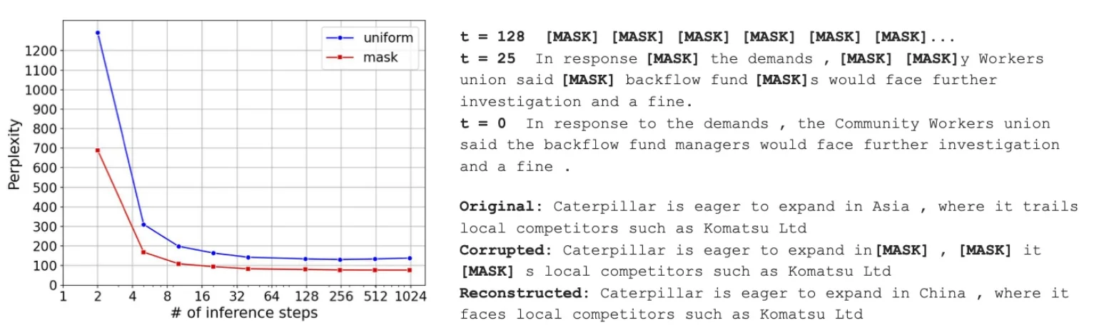
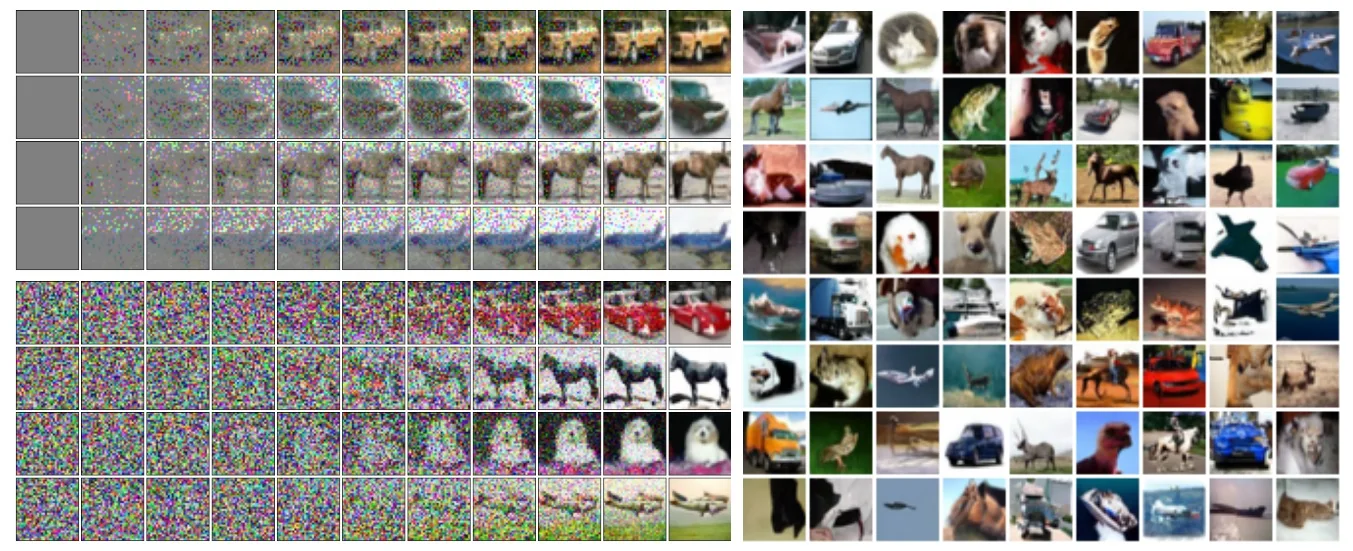
Experiments and Ablations: Match the Transition Prior to the Domain The empirical results of D3PM conclusively demonstrate that the choice of the forward transition matrix \(Q_t\) is not arbitrary; it must fundamentally align with the inherent structure of the target data domain [18]:
- Text Generation (The Triumph of the Absorbing State): For language modeling (evaluated on character-level text8 and word-level LM1B), the absorbing state ([MASK]) model drastically outperformed uniform diffusion. This confirms that iteratively revealing masked tokens is a far superior generative prior for language than attempting to correct uniformly randomized, unstructured words.
- Image Generation (The Necessity of Ordinality): On CIFAR-10, the Discretized Gaussian matrix was the clear winner. Because images possess strict ordinality, injecting Gaussian-like local decay into the discrete steps preserved the continuous topography of the image manifold, allowing D3PM to achieve highly competitive FID scores and log-likelihoods.
- Loss Ablation: Training exclusively with the VLB (\(L_{\mathrm {vb}}\)) often yielded lower-fidelity, less coherent samples. The hybrid loss \(L_\lambda \) was paramount, significantly improving generation quality and stabilizing optimization across modalities.
- Not every “structure” helps: The paper also studies a nearest-neighbor transition for text, where locality is induced from embedding similarity. Empirically, this structure is not reliably beneficial: it only narrowly improves over uniform in some settings, and can even underperform uniform corruption on LM1B. The takeaway is that a transition prior must match the domain’s true notion of locality, not just an arbitrary similarity heuristic [18].
Transition: Escaping the Sequential Bottleneck and Embracing Flows D3PM brilliantly formalizes how generative masked modeling mathematically operates under the umbrella of discrete diffusion via the absorbing state. However, predicting reverse transitions step-by-step over hundreds of strict Markov iterations remains computationally burdensome.
If we isolate this absorbing state paradigm, we can rethink the decoding sequence entirely. This naturally leads us to explore how models like MaskGIT [77] abandon strict sequential, token-by-token unmasking in favor of massively parallel, confidence-based token generation.
Furthermore, while D3PM successfully adapted curved diffusion to discrete spaces, the broader generative landscape has recently shifted toward straight-line Ordinary Differential Equations (ODEs) via Flow Matching. The remainder of this chapter will explore how the field ultimately bridges these two evolutionary branches. We will see how continuous vector fields are applied to categorical data (Discrete Flow Matching [171]), how every continuous-time method discussed in this chapter is mathematically unified under a single operator-level framework (Generator Matching [238]), and finally, how the field departs from continuous time altogether to achieve native compatibility with modern autoregressive architectures (Transition Matching [579]).
Enrichment 20.11.22: MaskGIT: Bidirectional, Non-Autoregressive Generation
Motivation: The Sequential Bottleneck Before MaskGIT, most high-quality image transformers followed the NLP recipe: flatten an image into a 1D sequence of discrete tokens and generate tokens autoregressively in raster-scan order (left-to-right, top-to-bottom). This design imposes two intertwined bottlenecks.
(i) An unnatural ordering bias. Images are not inherently sequential: global layout and long-range structure are best inferred from bidirectional context, not a forced scanline order [77]. The raster prior is a modeling artifact, not a property of visual data.
(ii) Quadratic token lengths and linear-time decoding. If a tokenizer produces an \(h\times w\) latent grid, then the sequence length is \(N = hw\) (e.g., \(N=32\times 32=1024\)). Autoregressive decoding requires \(\Theta (N)\) sequential transformer evaluations per sample, which is not parallelizable over token positions. MaskGIT emphasizes this inefficiency with a concrete runtime comparison against an autoregressive baseline: for long token sequences (e.g., \(N=1024\)), autoregressive decoding can take on the order of tens of seconds on a single GPU, while MaskGIT keeps the number of sequential transformer passes fixed (typically \(T=8\)).
Relation to D3PM: Absorbing-State Diffusion as Iterative Unmasking The D3PM framework in Enrichment 20.11.20 shows that discrete diffusion can be defined via a forward Markov chain with a mask absorbing state, yielding a “generate by iterative unmasking” reverse process [18]. MaskGIT is best understood as an aggressively optimized instantiation of this masked discrete generation paradigm:
- Common core: both begin from a fully corrupted canvas of [MASK] tokens and iteratively replace masks with data tokens.
- Different training objective: D3PM is derived as a Markovian diffusion model trained via an ELBO and an \(x_0\)-parameterized reverse process [18], whereas MaskGIT trains a bidirectional transformer with a direct masked-token cross-entropy objective (MVTM), analogous to BERT-style masked modeling [77, 121].
- Different sampler: D3PM samples according to diffusion-style reverse transitions; MaskGIT uses a scheduled parallel decoding heuristic that predicts all tokens in parallel and only commits the most confident subset at each iteration [77].
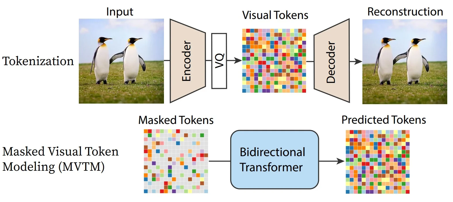
Stage 1: Tokenization into Discrete Visual Tokens MaskGIT mitigates the computational bottlenecks of high-resolution image generation by adopting the proven two-stage “tokenize-then-model” paradigm [77]. Because self-attention mechanisms scale quadratically with sequence length, operating directly on raw, continuous pixels is computationally prohibitive. Instead, the first stage utilizes a pretrained Vector Quantized (VQ) autoencoder (e.g., VQGAN-style) to compress the spatial dimensions of an input image \(x\in \mathbb {R}^{H\times W\times 3}\).
The encoder compresses the image by a fixed factor of 16 in the paper’s experimental setup, mapping \(x\in \mathbb {R}^{H\times W\times 3}\) to a grid of tokens with \(h=H/16\) and \(w=W/16\) [77]. Each token is an integer index into a learned codebook; MaskGIT uses a single codebook of size \(K=1024\) for its experiments. For transformer processing, this spatial grid is flattened into a 1D sequence \(Y=[y_i]_{i=1}^N\), where the total sequence length is \(N=hw\).
Stage 2: Masked Visual Token Modeling (MVTM) in Training With the image converted into a discrete sequence, MaskGIT trains a bidirectional transformer to play a visual “fill-in-the-blanks” game, a process termed Masked Visual Token Modeling (MVTM).
Let \(M=[m_i]_{i=1}^N \in \{0,1\}^N\) be a binary mask, where \(m_i=1\) indicates that the original token \(y_i\) is replaced by a special [MASK] token. Denoting the masked sequence as \(Y_M\), the transformer uses multi-head bidirectional self-attention to infer the missing patches.
Understanding Bidirectional Self-Attention. In a standard autoregressive transformer (such as GPT or early image transformers like ImageGPT), the self-attention mechanism employs a lower-triangular causal mask. This forces the computation of the attention score for token \(i\) to strictly depend only on preceding tokens \(j < i\). For images, this enforces an arbitrary raster-scan ordering (e.g., from top-left to bottom-right).
Conversely, a bidirectional transformer (like BERT or MaskGIT) removes this causal mask. The attention matrix is fully dense, meaning the contextualized representation of token \(i\) is computed as a weighted sum of all tokens \(j \in [1, N]\) in the sequence, looking both forward and backward.
Example: Consider generating an image of a dog in the bottom-left corner looking up at a flying frisbee in the top-right corner. If the visual token corresponding to the frisbee is masked, an autoregressive model must guess what belongs in that top-right patch before it has mathematically processed the dog in the bottom-left. It lacks the critical semantic context. A bidirectional transformer, however, processes the entire canvas simultaneously. The self-attention layers compute a high affinity between the masked token’s position and the unmasked tokens of the dog looking upward, allowing the network to trivially infer that the missing top-right patch should contain the frisbee.
Unlike autoregressive models that are strictly constrained to looking at past tokens in a raster-scan order, this bidirectional context allows the model to leverage unmasked tokens from all directions across the image to make highly informed predictions.
The model is optimized using a standard negative log-likelihood (cross-entropy) objective, calculating the loss exclusively on the masked locations:
\begin {equation} \mathcal {L}_{\mathrm {mask}} = -\mathbb {E}_{Y\sim \mathcal {D}} \left [ \sum _{i:\,m_i=1}\log p_\theta \!\left (y_i \mid Y_M\right ) \right ]. \label {eq:chapter20_maskgit_Lmask} \end {equation}
A crucial mathematical and practical element of this training stage is dynamic masking. Rather than using a fixed masking rate (like BERT’s static 15%), MaskGIT randomly samples a mask ratio \(r \in [0,1)\) at each training step via a continuous scheduling function \(\gamma (r)\). It then uniformly selects \(\lceil \gamma (r)\cdot N\rceil \) tokens to replace with masks.
This robust training strategy forces the model to learn how to recover visual information across a wide spectrum of corruption levels—ranging from inferring minor local details when the mask ratio is low, to hallucinating global structural layouts from near-scratch when the mask ratio is high.
Iterative Parallel Decoding (Inference) MaskGIT dismantles the autoregressive bottleneck by synthesizing an image in a constant, remarkably small number of iterations (typically \(T=8\)) [77]. This non-autoregressive parallel decoding algorithm leverages the bidirectional nature of the trained transformer to refine the entire canvas simultaneously. The algorithm’s mechanics are best understood by tracking the tensor shapes and probability distributions across a single iteration \(t\).
State Initialization and Representation. At inference, generation begins from a completely blank canvas where all \(N\) tokens are set to the [MASK] token, denoted as \(Y_M^{(0)}\). At any subsequent iteration \(t\), the canvas \(Y_M^{(t)} \in (\{1,\dots ,K\} \cup \{\texttt{[MASK]}\})^N\) contains a hybrid mixture of previously committed visual tokens and remaining masks. A single forward pass of the bidirectional transformer analyzes this partially filled canvas and outputs a categorical probability distribution over the entire \(K\)-dimensional codebook for every single position simultaneously: \begin {equation} P^{(t)} = p_\theta \!\left (\cdot \mid Y_M^{(t)}\right ) \in [0,1]^{N \times K}, \qquad \sum _{k=1}^K P^{(t)}_{ik} = 1. \label {eq:chapter20_maskgit_probs_shape} \end {equation}
Sample, Score, and Re-mask (The Confidence Heuristic). Unlike standard greedy sequential decoding, MaskGIT introduces a highly optimized heuristic based on the model’s own predictive confidence. For each currently masked position \(i\), a proposed token \(\hat {y}_i^{(t)}\) is stochastically sampled from the predicted distribution: \(\hat {y}_i^{(t)} \sim \mathrm {Cat}(P^{(t)}_{i:})\) [77].
In practice, this sampling incorporates temperature annealing to encourage more diversity [77].
Once a token is sampled, its corresponding predicted probability is extracted to serve as a ”confidence score”:
\begin {equation} c_i^{(t)} = P^{(t)}_{i,\hat {y}_i^{(t)}} \in [0,1]. \label {eq:chapter20_maskgit_confidence} \end {equation}
Tokens that are already committed (unmasked) in the current iteration automatically bypass this sampling and are assigned a maximum confidence of \(c_i^{(t)} = 1.0\).
At this stage, the model has a proposed token and a confidence score for every single position on the grid. To decide which predictions to permanently lock in, MaskGIT consults a mask scheduling function \(\gamma :[0,1] \to [0,1]\) [77]. This function determines the exact number of tokens \(n_t\) that must remain masked at the current fractional progress \(t/T\) [77]:
\begin {equation} n_t = \left \lceil \gamma \!\left (\frac {t}{T}\right ) N \right \rceil . \label {eq:chapter20_maskgit_nt} \end {equation}
To form the next input canvas \(Y_M^{(t+1)}\), the algorithm aggressively filters the proposals: it masks out the \(n_t\) positions holding the lowest confidence scores \(c_i^{(t)}\), and permanently commits the remaining high-confidence tokens. By locking in these reliable anchors first, the model drastically enriches the bidirectional context available for the next forward pass, allowing it to progressively and accurately resolve harder, localized details.
# MaskGIT scheduled parallel decoding (one sample).
# Y is an N-length token grid; K is codebook size; gamma controls the mask ratio.

Y = [MASK] * N                          # Y_M^{(0)}
for t in range(T):
    P = transformer_probs(Y)            # shape: (N, K)
    Y_hat = sample_tokens(P, temp=tau(t))  # sample for masked positions
    c = confidence(P, Y_hat, Y)         # c_i = P[i, Y_hat[i]] if masked else 1.0
    n = ceil(gamma(t / T) * N)          # number of tokens to KEEP masked
    idx = argsort(c)[:n]  # lowest-confidence positions
    Y = commit_and_remask(Y, Y_hat, idx)  # mask idx, commit others
# decode tokens back to pixels via VQ decoder
x = vq_decoder(Y)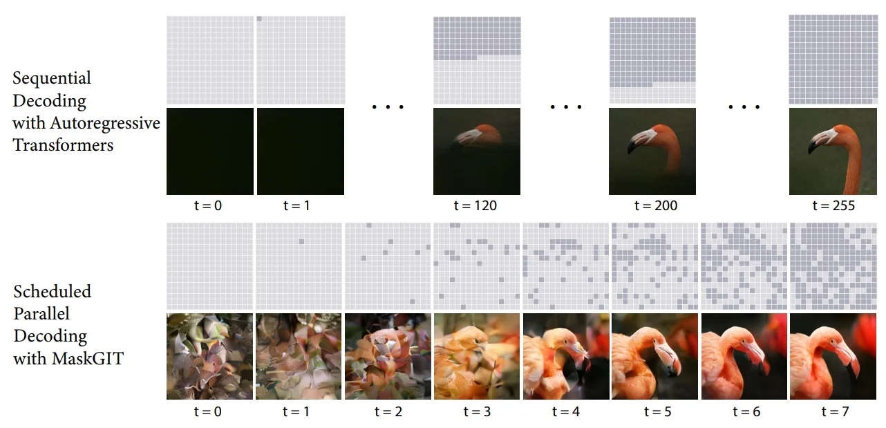
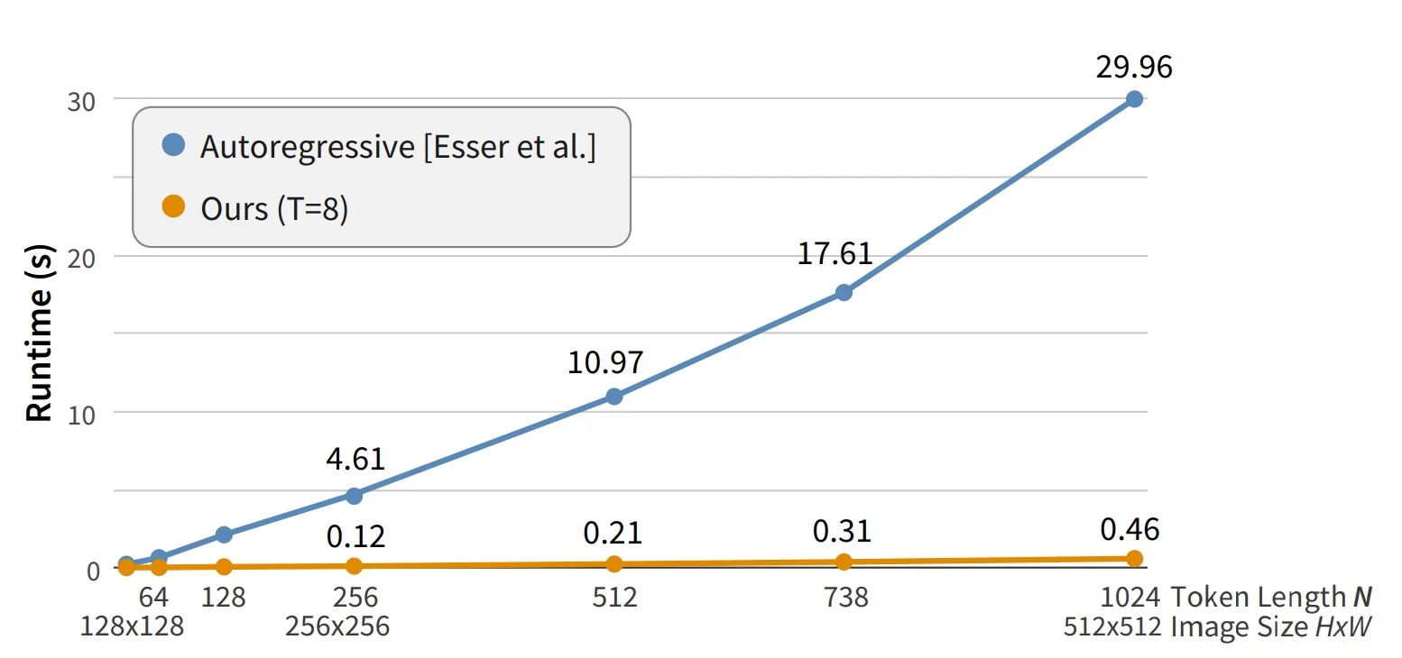
The Secret Sauce: The Mask Scheduling Function \(\gamma \) The schedule \(\gamma (\cdot )\) is used both in training (to sample corruption levels) and in inference (to decide how aggressively to re-mask). MaskGIT analyzes basic requirements for \(\gamma (r)\): it should be continuous and bounded in \([0,1]\), monotonically decreasing in \(r\), and satisfy \(\gamma (0)\to 1\) and \(\gamma (1)\to 0\); the monotone-decrease/boundary behavior ensures convergence of the iterative decoding procedure. Empirically, concave schedules perform best; MaskGIT reports that the cosine schedule is the strongest across their experiments [77]. For concreteness, one simple cosine-family instantiation that satisfies the required boundary conditions is \begin {equation} \gamma (r) \;=\; \cos \!\left (\frac {\pi }{2}r\right ), \qquad r\in [0,1], \label {eq:chapter20_maskgit_cosine} \end {equation} though other concave “cosine-like” variants are also possible.
Inherent Flexibility: Editing by Conditional Masking Because generation is bidirectional and conditioning is implemented simply by which tokens are initially masked, MaskGIT natively supports a family of image manipulation tasks without architectural changes. We keep the tokens corresponding to the unedited region fixed (unmasked) and set the edited region as the initial mask, then run the same iterative decoding algorithm:
- Class-conditional editing: mask a bounding box and condition on a target class to replace the object inside the box while preserving outside context.
- Inpainting and outpainting: treat missing (or extrapolated) regions as masks and iteratively fill them using surrounding context.
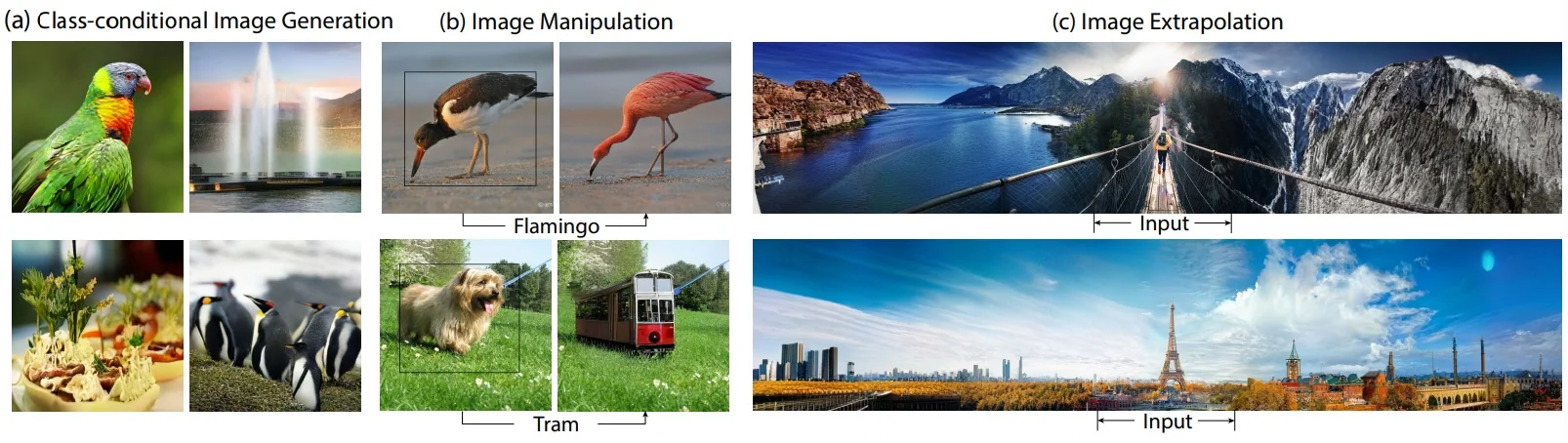
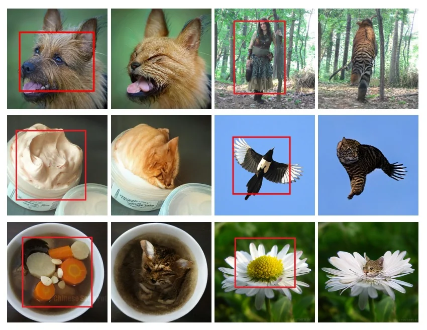
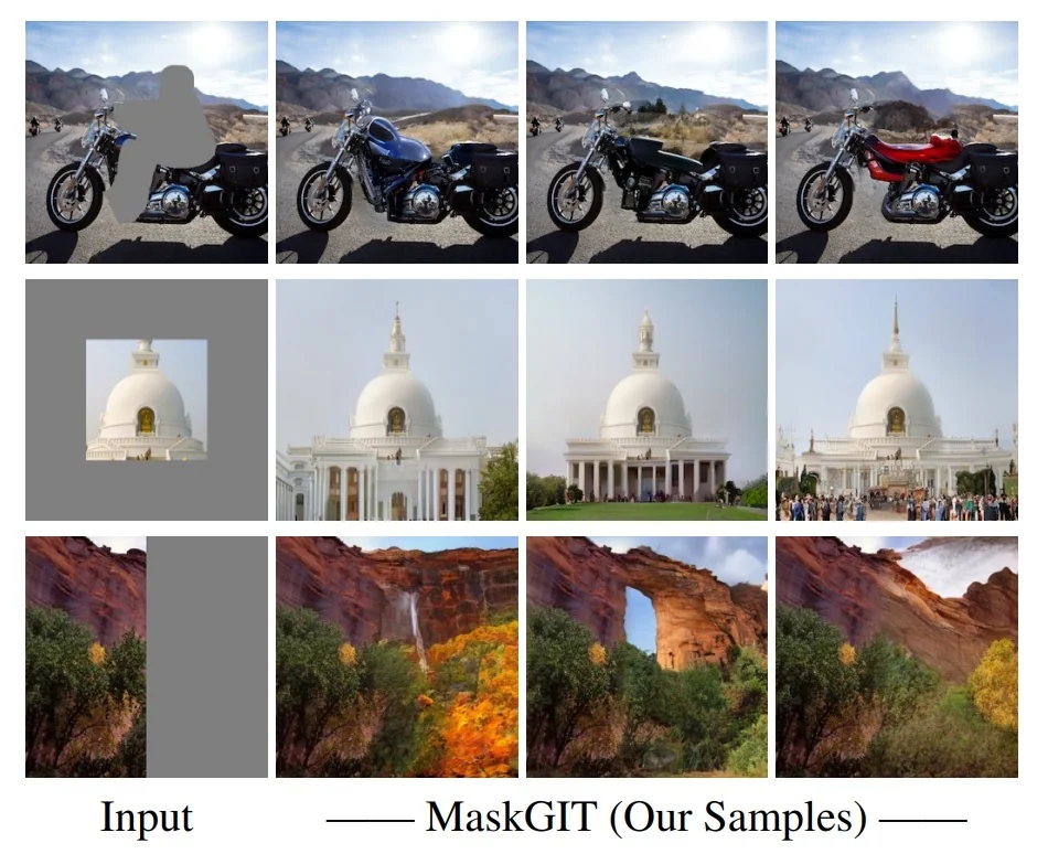
Transition: From Masked Discrete Diffusion to Flow-Based Discrete Generation MaskGIT shows that the absorbing-state “iterative unmasking” view highlighted by D3PM can be turned into an extremely fast sampler by combining (i) bidirectional masked-token prediction and (ii) a carefully designed confidence-based mask schedule. However, MaskGIT’s decoding is still an iterative refinement procedure, and its schedule is a heuristic that is not derived from a continuous-time generative dynamics. This sets up the next step in the chapter: flow-based formulations for discrete data that replace diffusion-style refinement with straight-line generator dynamics (e.g., Discrete Flow Matching and its modern extensions), providing a complementary route to fast sampling and scalable training.
Enrichment 20.11.23: DFM: Discrete Flow Matching
Motivation: From Heuristic Unmasking to Continuous-Time Flows The preceding enrichments established a practical recipe for discrete generation: D3PM (Enrichment Enrichment 20.11.20) provides a principled discrete-time Markov corruption process with an absorbing [MASK] variant [18], and MaskGIT (Enrichment Enrichment 20.11.21) turns iterative unmasking into a fast parallel sampler via a confidence-based schedule [77]. However, MaskGIT’s sampling rule—commit the most confident tokens, re-mask the rest—is a heuristic decoding policy rather than a generative dynamics derived from a continuous-time law. This distinction becomes practically relevant at a higher Number of Function Evaluations (NFE): the confidence-based commitment mechanism introduces a bias that, as the authors of DFM show empirically, can make sample quality non-monotonic in NFE—often plateauing and sometimes worsening—rather than consistently improving with finer discretization [171].
Discrete Flow Matching (DFM) [171] addresses this by translating the continuous Flow Matching framework [373] to categorical spaces. Rather than relying on discrete-time reverse kernels (as in diffusion) or confidence-based unmasking (as in MaskGIT), DFM defines a continuous-time generative process on a discrete state space via a Continuous-Time Markov Chain (CTMC). The model learns a time-dependent probability velocity that governs how probability mass moves between discrete states—a direct analogue of ODE-based vector fields, but for tokens. This CTMC formulation also lays the groundwork for Generator Matching [238] (a unifying mathematical framework for all continuous-time generative dynamics) and Transition Matching [579] (a departure to discrete time for LLM-scale architectures), discussed in later enrichments.
Road map. Before diving into the technical details, here is the high-level structure of DFM in a single pass:
- 1.
- Setup — define the discrete state space, pair each noise sample with a data sample via a coupling \(\pi \), and connect them with a continuous-time probability path (the convex interpolant).
- 2.
- Continuity equation — establish the conservation law that any valid probability velocity must satisfy.
- 3.
- CTMC update — translate the velocity into a concrete sampling rule: at each time step, form a categorical distribution and sample the next token from it (this is where the stochasticity enters).
- 4.
- Velocity construction — derive a closed-form velocity from a learned probability denoiser \(p_{1|t}\); the network never predicts velocities directly but rather predicts “what is the clean token?”, and the velocity is computed from that prediction.
- 5.
- Training — show that learning the denoiser reduces to a standard token-wise cross-entropy loss, with no CTMC simulation required during training.
- 6.
- Sampling — simulate the CTMC forward from noise to data using the learned velocity.
Setup: State Spaces, Couplings, and Probability Paths To translate continuous flows to discrete data, DFM must define three ingredients: a state space, a way to pair noise with data, and a continuous-time path connecting the two.
- 1.
- Discrete state space. The domain is \(\mathcal {D} = [d]^N\), where \(d\) is the number of
categories each token can take and \(N\) is the sequence length. Each
element \(x \in \mathcal {D}\) is an \(N\)-tuple of categorical tokens, with every token drawn
from the alphabet \(\{1,2,\dots ,d\}\).
What \(d\) represents depends on the data modality. For text, \(d\) is the vocabulary size of the tokenizer (e.g., \(d \approx 50{,}000\) for a BPE vocabulary). For images, the standard pipeline first encodes the continuous image into a grid of discrete visual tokens using a Vector Quantized (VQ) autoencoder (e.g., VQGAN [149]), and \(d\) is the size of the learned codebook—MaskGIT, for instance, uses \(d = K = 1024\) (see Enrichment Enrichment 20.11.21). Alternatively, when operating directly on raw pixel intensities without a learned tokenizer, \(d = 256\) (one category per gray-level or per-channel color value). The sequence length \(N\) is the total number of tokens: for a VQ-encoded image with spatial compression factor 16, \(N = (H/16)\times (W/16)\).
Image example: from pixels to token sequences. A \(256\times 256\) RGB image enters the VQ encoder, which compresses it spatially by a factor of 16 and maps each \(16\times 16\) patch to its nearest codebook entry. The output is a grid of \(16\times 16 = 256\) integer token indices, each drawn from the codebook \(\{1,2,\dots ,1024\}\). From DFM’s perspective, this is simply a sequence of \(N=256\) tokens with \(d=1024\) categories—exactly the same mathematical object as a 256-token sentence with a 1024-word vocabulary. A CTMC “jump” for one of these visual tokens means switching from one codebook entry to another (e.g., from a blue-sky patch embedding to a cloud patch embedding), not a gradual pixel-level blend. After generation, the VQ decoder maps the token grid back to pixel space, producing the final image.
- 2.
- Source–target coupling \(\pi \). DFM transforms a source distribution \(p\)
(e.g., all-[MASK] tokens or uniform noise) into a target distribution \(q\)
(the data). The two are linked by a joint coupling \(\pi (x_0, x_1)\)—a joint distribution
whose marginals are \(x_0 \sim p\) and \(x_1 \sim q\). Concretely, \(\pi \) answers the question: “given
a training example \(x_1\) from the dataset, which noise sample \(x_0\) should
it be paired with?”. Note that the coupling is not learned; it is a
fixed design choice made before training begins and kept constant
throughout. In practice, constructing a sample from \(\pi \) during training
simply means: (i) draw a data sample \(x_1\) from the training set (this is the
“label”), and (ii) draw a noise sample \(x_0\) independently from the source
distribution \(p\). The coupling then appears in the loss (Equation 20.173)
as the outer expectation \(\mathbb {E}_{(x_0,x_1)\sim \pi }\).
For unconditional generation the coupling is independent: \(\pi (x_0,x_1) = p(x_0)\,q(x_1)\), meaning the noise sample and the data sample are drawn without any positional correspondence. This is the simplest and most common case: it requires no labeling, no alignment, and no supervision beyond having a dataset of token sequences and a choice of source distribution.
For conditional tasks (infilling, prefix completion, constrained generation), DFM uses a Conditional Coupling (C-Coupling) that bakes the condition into the source endpoint. Let \(I\in \{0,1\}^N\) be an indicator mask of conditioned positions (known context), and let \(\mathfrak {m}\) denote the source token (e.g., [MASK]). The coupling samples \(x_1\sim q\) and defines the source endpoint as
\begin {equation} x_0 \;=\; I\odot x_1 + (1-I)\odot (\mathfrak {m},\ldots ,\mathfrak {m}), \label {eq:chapter20_dfm_c_coupling} \end {equation}
so conditioned positions are already correct at \(t=0\) and remain fixed along the trajectory. At inference time, we enforce the same constraint by clamping after each CTMC step. Let \(Y\in [d]^N\) denote the fixed context tokens (e.g., the prompt prefix or the unmasked image region). The clamping operator \begin {equation} \mathrm {Clamp}(X;\,Y,I) \;=\; I\odot Y + (1-I)\odot X \label {eq:chapter20_dfm_clamp} \end {equation} is applied after every Euler step, overwriting the conditioned positions with their known values and ensuring the flow acts only on the unconditioned coordinates [171].
For example, in image inpainting, \(I\) marks the unmasked pixel positions; in text completion, \(I\) marks the prompt prefix.
- 3.
- Probability path. In continuous Flow Matching (Enrichment Enrichment 20.9.11),
the generative path is a deterministic ODE: each sample point \(x \in \mathbb {R}^N\) slides along
a vector field from a noise location to a data location. DFM must translate
this idea to a setting where intermediate fractional states between two
discrete tokens do not exist—there is no “halfway point” between the word
cat and the word dog.
The solution is to shift the continuous dynamics from the states themselves to distributions over those discrete states. DFM defines a continuous-time probability path \(\{p_t\}_{t\in [0,1]}\) that smoothly interpolates from \(p_0 = p\) (noise) to \(p_1 = q\) (data). At each time \(t\), \(p_t\) assigns a probability to every element of the discrete space \(\mathcal {D}\); it is this probability mass—not any individual token—that evolves continuously. The path is constructed in two steps: first define a conditional path \(p_t(\cdot \mid x_0, x_1)\) anchored at a specific noise–data pair, then marginalize over the coupling:
\begin {equation} p_t(x) \;=\; \sum _{x_0,x_1 \in \mathcal {D}} p_t(x \mid x_0, x_1)\,\pi (x_0, x_1). \label {eq:chapter20_dfm_marginal_path} \end {equation}
For scalability to high dimensions, DFM assumes the conditional path factorizes across coordinates: \(p_t(x \mid x_0, x_1) = \prod _{i=1}^N p_t^i(x^i \mid x_0^i, x_1^i)\). Each token’s distribution evolves independently given its paired endpoints—the same factorization principle that makes D3PM and MaskGIT tractable.
The convex interpolant. A natural and widely used choice for the per-token conditional path is the two-point convex interpolation:
\begin {equation} p_t^i(x^i \mid x_0^i, x_1^i) \;=\; \kappa _t\,\delta _{x_1^i}(x^i) + (1-\kappa _t)\,\delta _{x_0^i}(x^i), \qquad \kappa _0=0,\;\kappa _1=1. \label {eq:chapter20_dfm_convex_path} \end {equation}
In words: at time \(t\), each token is either still in its source state \(x_0^i\) (with probability \(1-\kappa _t\)) or has already jumped to its target state \(x_1^i\) (with probability \(\kappa _t\)). There is no gradual morphing or blending of token identities—a token is purely in one state or the other—but the probability of having made the jump increases smoothly from 0 to 1. This is the discrete counterpart of the continuous interpolant \(x_t = (1-t)\,x_0 + t\,x_1\) in Euclidean Flow Matching: where the continuous version slides a point along a straight line, the discrete version smoothly increases the chance that each token has switched from noise to data. The function \(\kappa _t\) acts as a scheduler—the discrete analogue of a noise schedule in continuous diffusion—controlling the rate at which tokens probabilistically transition from noise toward data.
Unpacking the delta notation. The symbol \(\delta _{x_1^i}(x^i)\) is a Kronecker delta—a discrete “one-hot” indicator that equals 1 when its argument matches the subscript and 0 otherwise: \[ \delta _{a}(x) \;=\; \begin {cases} 1 & \mbox{if } x = a,\\ 0 & \mbox{if } x \neq a.\end {cases} \] To see this concretely, consider a toy vocabulary of \(d=3\) tokens: \(\{\texttt{A}, \texttt{B}, \texttt{C}\}\). During training, we draw a data sample \(x_1\) from the dataset and independently draw a noise sample \(x_0\) from the source distribution (as specified by the coupling \(\pi \)).
Suppose the source (noise) token at position \(i\) is \(x_0^i = \texttt{A}\) (e.g., drawn uniformly from \(\{\texttt{A},\texttt{B},\texttt{C}\}\)) and the target (clean) token from the training data is \(x_1^i = \texttt{C}\). Then \(\delta _{x_1^i} = \delta _{\texttt{C}}\) is the one-hot vector \([0,\,0,\,1]\) (all mass on C), and \(\delta _{x_0^i} = \delta _{\texttt{A}}\) is \([1,\,0,\,0]\). At time \(t\) with scheduler value \(\kappa _t = 0.3\), the convex interpolant (20.164) gives \[ p_t^i \;=\; 0.3\cdot [0,\,0,\,1] \;+\; 0.7\cdot [1,\,0,\,0] \;=\; [0.7,\,0,\,0.3]. \] The token has a 70% chance of still being A (noise) and a 30% chance of having jumped to C (data). No probability mass lands on B, because the two-point interpolant only moves mass between the paired source and target categories. As \(\kappa _t\) increases from 0 to 1, the distribution smoothly shifts from \([1,\,0,\,0]\) (pure noise) to \([0,\,0,\,1]\) (pure data).
Analogy with DDPM noise schedules. Students familiar with continuous diffusion will recognize the parallel immediately. In DDPM (Enrichment Enrichment 20.9.1), the cumulative schedule \(\bar {\alpha }_t = \prod _{s=1}^{t}\alpha _s\) controls the ratio of signal to noise at time \(t\): the closed-form forward kernel is \(\mathbf {x}_t = \sqrt {\bar {\alpha }_t}\,\mathbf {x}_0 + \sqrt {1-\bar {\alpha }_t}\,\boldsymbol {\varepsilon }\), so \(\bar {\alpha }_t\) continuously interpolates between the original image coordinates and Gaussian noise.
In DFM, \(\kappa _t\) plays the same role, but for probability mass over categories rather than spatial coordinates: it continuously interpolates between the probability of being in the source state and the probability of being in the target state.
The instantaneous rate also has a direct counterpart. In continuous-time diffusion, the per-step noise injection is governed by \(\beta (t)\); in DFM, the time derivative \(\dot {\kappa }_t\) fills this role. As we will see in the velocity formula, the factor \(\dot {\kappa }_t/(1-\kappa _t)\) scales the denoiser’s output at each instant, dictating how fast probability mass flows between categories at that moment.
Schedule design. Just as the diffusion community found that a linear \(\beta _t\) schedule destroys images too aggressively—leading to the cosine schedule of Nichol and Dhariwal [463]—DFM requires careful tuning of \(\kappa _t\). The simplest choice is a linear scheduler \(\kappa _t = t\), which transitions tokens at a constant rate. DFM also studies a cosine schedule \(\kappa _t = 1-\cos (\tfrac {\pi }{2}t)\) and, more importantly, a cubic-polynomial family
\begin {equation} \kappa _t \;=\; -2t^3 + 3t^2 +\; a\,(t^3-2t^2+t) +\; b\,(t^3-t^2), \label {eq:chapter20_dfm_kappa_cubic} \end {equation}
which satisfies \(\kappa _0=0\) and \(\kappa _1=1\) for any \(a,b\). The parameters \(a\) and \(b\) directly control the boundary derivatives \(\dot {\kappa }_0 = a\) and \(\dot {\kappa }_1 = b\), providing a principled way to shift transition mass earlier or later in the trajectory. Setting \(a{=}0,\,b{=}2\) recovers the quadratic schedule \(\kappa _t = t^2\); the base case \(a{=}b{=}0\) gives the Hermite smoothstep \(3t^2-2t^3\). The authors ablate across these families and find that non-linear schedules (the “FM-Cubic” variants) yield substantially better FID and generative perplexity; in practice, schedules that concentrate transitions in the mid-range of the trajectory, where the denoiser’s predictions are most informative, outperform the linear baseline (see the ablation discussion below) [171].
Practical benefit: simulation-free training. A key advantage of the convex interpolant is that it provides a closed-form expression for the distribution at any time \(t\). During training, we do not need to simulate the CTMC step by step to obtain corrupted samples. Instead, we sample a random time \(t\), draw endpoints \((x_0, x_1) \sim \pi \), and directly sample \(X_t\) from the convex interpolant—each token independently set to its target state with probability \(\kappa _t\) or its source state with probability \(1-\kappa _t\). This makes training fully parallelizable across both time and sequence positions, identical in spirit to the simulation-free regime of continuous Flow Matching.
The Discrete Continuity Equation: Probability Mass Conservation on \(\mathcal {D}\) We now have a probability path that smoothly interpolates between noise and data. The next step is to identify the mathematical law that governs how probability mass moves along this path. Because tokens can only undergo discrete jumps (from one category to another), probability mass is literally flowing between categories over time. For the generative process to be mathematically consistent, this flow must conserve probability: mass cannot appear from or vanish into nowhere.
In continuous Flow Matching, this conservation is enforced by the continuity equation \(\dot {p}_t(x) + \mathrm {div}(p_t u_t) = 0\), where the divergence operator measures the spatial spread of a vector field \(u_t\) [373]. DFM shows that the same conservation law governs discrete flows, but divergence must be redefined: in a discrete space, there is no spatial derivative, so divergence instead becomes a net flux balance—the total outgoing probability flux leaving a specific discrete state minus the incoming flux entering it.
Formally, for a flux function \(v:\mathcal {D}\times \mathcal {D}\to \mathbb {R}\), the discrete divergence at state \(x\) is
\begin {equation} \mathrm {div}_x(v) \;=\; \sum _{z\in \mathcal {D}} \big (v(z,x)-v(x,z)\big ). \label {eq:chapter20_dfm_discrete_div} \end {equation}
Following the velocity convention (destination, source), each term \(v(z,x)\) represents the flow of probability out of \(x\) toward state \(z\), while \(v(x,z)\) represents the flow into \(x\) from \(z\); the sum thus gives the net outgoing flux from state \(x\). The discrete continuity equation then states that the rate of change of probability at any state must exactly balance this net flux:
\begin {equation} \dot {p}_t(x) \;+\; \mathrm {div}_x\!\big (p_t u_t\big ) \;=\; 0, \label {eq:chapter20_dfm_discrete_continuity} \end {equation}
where \(u_t\) is a probability velocity that specifies how probability mass moves between states. In plain terms: if the probability of a particular sequence increases by some amount, that exact amount must have been drained away from other sequences. The velocity \(u_t\) governs these transfers, and Equation 20.167 guarantees that no probability is created or destroyed.
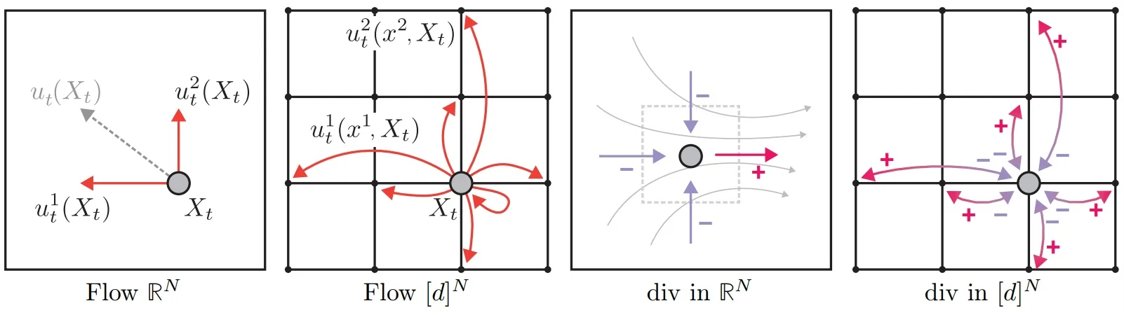
From Vector Fields to Probability Velocities: A CTMC Update Rule DFM generates samples by simulating a Continuous-Time Markov Chain (CTMC) over \(\mathcal {D}\). The key idea is simple: at each time step, the model predicts a denoiser distribution (“what is the clean token?”) at every position; this prediction is then converted into a probability velocity via a closed-form formula, and the velocity is used to construct a categorical transition distribution from which we randomly sample the next token. This random sampling is the source of stochasticity in DFM’s generative process—unlike continuous Flow Matching, where the ODE integrator is deterministic once the initial noise is fixed, each CTMC step involves a genuine random draw.
In continuous Flow Matching, the velocity \(u_t(x)\) is a vector in \(\mathbb {R}^N\) pointing in a spatial direction. In the discrete setting, there are no spatial directions; instead, “velocity” means the rate at which probability is shifting between categories.
Reading the notation. For a current state \(z\in \mathcal {D}\), the quantity \(u_t^i(x^i, z)\) is a rate (units: probability per unit time). When \(x^i \neq z^i\), the value \(u_t^i(x^i,z) \ge 0\) is the instantaneous jump rate from the current category \(z^i\) to the candidate category \(x^i\) at position \(i\), conditioned on the full sequence \(z\). The superscript \(i\) indexes the token position (e.g., the 5th word in a sentence or the 5th patch in an image grid); the argument \(z\) (also written \(X_t\)) is the full current state, which the neural network inspects to produce context-dependent predictions; and \(x^i\) ranges over the vocabulary \([d]\). The diagonal entry \(u_t^i(z^i, z)\) is the negative sum of all outgoing rates, so that total mass is conserved: it is the “drain” that balances the outgoing flow.
The CTMC update. Let \(X_t\sim p_t\) be the random state at time \(t\). Over a small step \(h>0\), DFM updates each token using the Euler-style CTMC rule (valid for sufficiently small \(h\))
\begin {equation} X_{t+h}^i \;\sim \; \delta _{X_t^i}(\cdot ) + h\,u_t^i(\cdot , X_t), \label {eq:chapter20_dfm_ctmc_update} \end {equation}
which says: form a categorical distribution by starting with all probability mass on the current category (\(\delta _{X_t^i}\) is the one-hot vector), then redistribute a small fraction of that mass according to the velocity. We then draw a random sample from this categorical distribution to obtain the next token \(X_{t+h}^i\). Concretely, if \(h\) is small, the token most likely stays where it is (the one-hot term dominates), but with small probability proportional to \(h\cdot u_t^i\), it jumps to a different category. As \(t\) advances and the velocity grows (via the speed prefactor), these jumps become increasingly probable, until by \(t\approx 1\) virtually all tokens have transitioned to their final states. The result is a valid categorical distribution over \([d]\) provided \(u_t^i\) satisfies the probability-velocity constraints:
\begin {equation} \sum _{x^i\in [d]} u_t^i(x^i,z)=0, \qquad u_t^i(x^i,z)\ge 0 \;\;\mbox{for all }x^i\neq z^i. \label {eq:chapter20_dfm_velocity_constraints} \end {equation}
The first condition ensures that probability is conserved (the rates sum to zero), and the second ensures that outgoing flow is non-negative for all categories other than the current state. In our three-token vocabulary \(\{\texttt{A},\texttt{B},\texttt{C}\}\), if the token currently occupies A, the velocity \(u_t^i\) has exactly one negative entry (at A, the drain) and non-negative entries at B and C (the pumps), with all three summing to zero. Unlike continuous ODE integration (which is deterministic once the initial noise is fixed), the CTMC update involves stochastic sampling from the categorical distribution at each step, making the generative process inherently random.
Step-size validity. Even when the velocity constraints hold, the step size \(h\) must be small enough that every entry of the categorical distribution \(\delta _{X_t^i}(\cdot ) + h\,u_t^i(\cdot , X_t)\) remains non-negative. The critical entry is the current-state probability: it equals \(1 + h\,u_t^i(z^i, z) = 1 - h\cdot [\mbox{sum of outgoing rates}]\), which goes negative if \(h\) is too large. Because the velocity is scaled by the speed prefactor \(\dot {\kappa }_t/(1-\kappa _t)\), which grows as \(t\to 1\), the maximum safe step shrinks near the end of the trajectory. DFM addresses this with an adaptive step size: \[ h_{\mathrm {adapt}} \;=\; \min \!\Big (h,\;\tfrac {1-\kappa _t}{\dot {\kappa }_t}\Big ). \] The bound \((1-\kappa _t)/\dot {\kappa }_t\) is exactly the reciprocal of the speed prefactor; choosing \(h\) no larger than this value guarantees that the one-hot term still dominates and all probabilities stay in \([0,1]\). In practice, this means the sampler takes its standard step size for most of the trajectory but automatically shortens steps near \(t=1\) [171].
The number of function evaluations (NFE) is the number of neural-network calls used to evaluate \(u_t\) along the trajectory, i.e., the number of discrete time steps in the CTMC simulation.
The Core Construction: A Tractable Velocity via a Learned Denoiser The CTMC update (20.168) tells us how to step forward given a velocity, and the continuity equation (20.167) tells us what a valid velocity must satisfy. The remaining question is: how do we construct such a velocity? DFM’s main technical result is that for broad path families, a generating velocity can be written in closed form once we know a single quantity: the probability denoiser \(p_{1|t}(x^i\mid z)\).
What is \(p_{1|t}\)? The notation \(p_{1|t}(x^i \mid z)\) reads: “the probability that the clean (target) token at position \(i\) is \(x^i\), given that the current noisy sequence is \(z\)”. In other words, it is a Bayesian posterior—if we observe the partially corrupted state \(z\) at time \(t\), what do we believe the original data token was? The subscript “\(1|t\)” emphasizes that we are predicting the endpoint at \(t{=}1\) (the clean data) conditioned on the state at time \(t\). This is the discrete analogue of \(x_0\)-prediction in continuous diffusion: the network does not predict a velocity or a noise vector; it predicts “what was the clean token?”, and DFM’s formula converts that prediction into a velocity automatically.
Operationally, the recipe is:
- 1.
- Choose a conditional probability path \(p_t(\cdot \mid x_0,x_1)\) (e.g., the convex path in (20.164)) and a scheduler \(\kappa _t\).
- 2.
- Train a neural network \(p_\theta (x^i \mid z, t)\) to approximate the true posterior \(p_{1|t}(x^i\mid z)\)—i.e., to predict the clean token from the noisy state.
- 3.
- At inference time, plug the network’s prediction into a closed-form velocity formula, then simulate the CTMC via (20.168).
For the convex path (20.164), DFM derives a particularly simple denoiser-parameterized marginal velocity:
\begin {equation} u_t^i(x^i,z) \;=\; \underbrace {\frac {\dot {\kappa }_t}{1-\kappa _t}}_{\mbox{speed (scheduler)}} \;\cdot \; \underbrace {\Big (p_{1|t}(x^i\mid z)-\delta _{z^i}(x^i)\Big )}_{\mbox{direction (neural network)}}, \label {eq:chapter20_dfm_velocity_denoiser} \end {equation}
where \(p_{1|t}(x^i\mid z)\) is the probability denoiser introduced above.
A crucial point: the neural network never predicts the velocity \(u_t\) directly. It predicts a categorical distribution over clean tokens (“what is the original data?”), and the velocity is computed from that prediction via the closed-form formula above. The speed prefactor and the subtraction of the current state are deterministic operations applied to the network’s output—no separate velocity network is needed. This formula splits cleanly into two roles:
- Direction (data-dependent). The term \(\big (p_{1|t}(x^i\mid z) - \delta _{z^i}(x^i)\big )\) is a signed vector over the vocabulary \([d]\). It subtracts the current token at position \(i\), represented by the one-hot \(\delta _{z^i}(x^i)\), from the denoiser’s distribution \(p_{1|t}(x^i\mid z)\). The result drains mass from the currently occupied category (the unique negative entry on the diagonal) and pumps it toward categories the denoiser deems likely (off-diagonal nonnegative entries).
- Speed (data-independent). The prefactor \(\dot {\kappa }_t/(1-\kappa _t)\) is determined entirely by the scheduler \(\kappa _t\) and does not depend on the data or the network. It acts as a global scaling factor that controls how fast probability mass is allowed to flow at time \(t\). Early in generation, \(1-\kappa _t \approx 1\) and the speed is moderate; late in generation, \(1-\kappa _t \to 0\) and the prefactor grows, forcing all remaining probability mass to complete the transition before the trajectory ends at \(t=1\).
Worked example: velocity for a three-token vocabulary. Returning to our \(\{\texttt{A}, \texttt{B}, \texttt{C}\}\) vocabulary, suppose at time \(t\) the token currently sits in state \(z^i = \texttt{A}\). The neural network inspects the full noisy sequence \(z\) and produces a categorical prediction \(p_{1|t}(\cdot \mid z) = [0.1,\, 0.7,\, 0.2]\), indicating that the clean token is most likely B. The current state as a one-hot vector is \(\delta _{\texttt{A}} = [1,\,0,\,0]\). The direction term in (20.170) is then \[ p_{1|t} - \delta _{z^i} \;=\; [0.1,\, 0.7,\, 0.2] - [1,\,0,\,0] \;=\; [-0.9,\, +0.7,\, +0.2]. \] This signed vector is an explicit instruction: drain 0.9 units of probability from the current category A (the only negative entry), and pump it toward B (+0.7) and C (+0.2). The entries sum to zero, consistent with the conservation constraint (20.169). Multiplying by the speed prefactor \(\dot {\kappa }_t/(1-\kappa _t)\) scales this instruction to the appropriate magnitude for the current time.
Speed prefactor: concrete numbers. Consider the linear scheduler \(\kappa _t = t\), so \(\dot {\kappa }_t = 1\). The speed prefactor is \(1/(1-t)\). At \(t=0.1\) (early in generation), the prefactor is \(1/(1-0.1) = 1/0.9 \approx 1.11\)—the velocity is close to the raw direction. At \(t=0.5\) (halfway), it doubles to \(1/0.5 = 2.0\). At \(t=0.9\) (near the end), it surges to \(1/0.1 = 10.0\). At \(t=0.99\), it reaches \(1/0.01 = 100\). This divergence is not pathological—it is the mechanism that ensures all remaining undecided tokens complete their transitions before the trajectory ends. By \(t=0.9\), a token that has not yet jumped to its target is increasingly rare (\(1-\kappa _t = 0.1\)), so the velocity must intensify to push the remaining 10% of probability mass to its destination within the final 10% of the time budget.
A complementary noise-prediction form is \begin {equation} u_t^i(x^i,z) \;=\; \frac {\dot {\kappa }_t}{\kappa _t} \Big (\delta _{z^i}(x^i)-p_{0|t}(x^i\mid z)\Big ), \label {eq:chapter20_dfm_velocity_noisepred} \end {equation}
which mirrors the denoiser/noise duality familiar from diffusion (\(\epsilon \)- vs. \(x_0\)-style parameterizations), but now expressed as probability velocities [171].
Corrector Sampling: Reintroducing Noise Without Heuristic Commitment The basic CTMC sampler is analogous to an ODE solver in continuous Flow Matching: it traces the probability path forward without injecting additional randomness beyond the categorical sampling at each step. In continuous diffusion, sample quality often improves when deliberate noise is injected during generation (e.g., Langevin corrector steps in score-based models). DFM introduces a discrete analogue: combine a forward-time velocity \(\hat {u}_t\) and a backward-time velocity \(\check {u}_t\) to build a new valid forward-time velocity
\begin {equation} \bar {u}_t^i(x^i,z) \;=\; \alpha _t\,\hat {u}_t^i(x^i,z) - \beta _t\,\check {u}_t^i(x^i,z), \qquad \alpha _t,\beta _t>0, \label {eq:chapter20_dfm_corrector_velocity} \end {equation}
which supports two regimes:
- Forward-plus-backward corrector (\(\alpha _t - \beta _t = 1\)): the effective step moves \((1+\beta _t)\) units forward and \(\beta _t\) units backward. Practically, this means the model may commit a token, then partially retract the decision based on updated context—analogous to “unmasking and re-masking” in MaskGIT, but governed by the probability velocity rather than a confidence heuristic. The net forward progress is one step, so the trajectory still generates \(\{p_t\}\).
- Fixed-\(t\) corrector (\(\alpha _t - \beta _t = 0\)): the forward and backward flows cancel, producing a chain whose stationary distribution is \(p_t\). Running several corrector sub-steps at a fixed time refines the current sample without advancing the clock, improving quality at critical time points.
In the forward-plus-backward regime, a common choice enforces \(\beta _t = \alpha _t - 1\) with a smooth schedule that concentrates corrector strength in the mid-trajectory (where predictions are most uncertain) and vanishes near the endpoints (where the path is near its boundary conditions). The authors ablate polynomial families for \(\alpha _t\) and find that moderate corrector strength improves both diversity and quality [171]. This replaces MaskGIT’s confidence-based commit/re-mask rule with a dynamics-grounded mechanism for diversity and refinement [171].
Training Objective: Flow Matching as Token-Wise Cross-Entropy With the velocity formula and corrector mechanism in hand, the remaining piece is how to train the denoiser \(p_\theta \) that drives the velocity. Because the convex interpolant provides a closed-form expression for \(p_t(\cdot \mid x_0, x_1)\), training is simulation-free—we never need to run the CTMC step by step to generate training examples. The procedure is fully parallelizable:
- 1.
- Sample endpoints: draw a clean target sequence \(x_1\) from the data and a noise sequence \(x_0\) from the source distribution \(p\).
- 2.
- Sample time: draw \(t \sim \mathcal {U}(0,1)\).
- 3.
- Instant corruption: construct the noisy state \(X_t\) by independently setting each token to its target value \(x_1^i\) with probability \(\kappa _t\), or its source value \(x_0^i\) with probability \(1-\kappa _t\). No iterative forward process is required.
- 4.
- Predict: feed \((X_t, t)\) into the neural network, which outputs a categorical distribution \(p_\theta (\cdot \mid X_t, t)\) over \([d]\) at every position.
- 5.
- Supervise: compute the loss by comparing the network’s prediction to the true clean tokens.
The resulting objective reduces to a standard token-wise cross-entropy:
\begin {equation} \mathcal {L}_{\mathrm {DFM}} = -\mathbb {E}_{(x_0,x_1)\sim \pi }\,\mathbb {E}_{t}\,\mathbb {E}_{X_t\sim p_t(\cdot \mid x_0,x_1)} \left [ \sum _{i=1}^N \log p_\theta \!\big (x_1^i \mid X_t, t\big ) \right ], \label {eq:chapter20_dfm_loss} \end {equation}
where the network is penalized for assigning low probability to the true clean token at each masked or corrupted position. Unlike D3PM’s ELBO (which supervises reverse transitions indirectly), DFM directly trains the denoiser that parameterizes the velocity used at inference. And unlike MaskGIT’s MVTM objective (Equation 20.156), which supervises only explicitly masked positions, DFM’s corruption is probabilistic (via \(\kappa _t\)) rather than binary, and the loss sums over all positions—including tokens that already equal their target.
Sampling Algorithm: Scheduled CTMC Simulation At inference time, we do not have access to the clean data; generation proceeds by simulating the CTMC forward from pure noise. The procedure is straightforward:
- 1.
- Initialize: start at \(t=0\) with a sequence \(X_0\) drawn entirely from the source distribution (e.g., all-[MASK] tokens). Choose the number of steps \(n\) (the NFE budget), giving a step size \(h = 1/n\).
- 2.
- Loop from \(t = 0\) to \(t = 1 - h\) in increments of \(h\):
- (a)
- Predict: pass the current sequence \(X_t\) and time \(t\) to the neural network to obtain \(p_\theta (\cdot \mid X_t, t)\).
- (b)
- Compute velocity: plug the prediction and the current scheduler values \((\kappa _t, \dot {\kappa }_t)\) into Equation 20.170 to obtain \(u_t^i(\cdot , X_t)\) for every token position.
- (c)
- Euler step: form the categorical distribution \(\delta _{X_t^i}(\cdot ) + h\,u_t^i(\cdot , X_t)\) and sample the next token \(X_{t+h}^i\) from it (Equation 20.168).
- (d)
- Clamp (conditional only): for conditional tasks, overwrite conditioned positions using \(X \leftarrow \mathrm {Clamp}(X;\,Y,I)\) (Equation 20.162).
- 3.
- Output: at \(t=1\), the sequence \(X_1\) is the generated sample.
# Discrete Flow Matching sampler (conceptual).
# Domain: tokens in [d]^N.  Denoiser predicts p_theta(x1^i | X_t, t).
# Velocity: u_t^i(., X_t) = (kappa_dot/(1-kappa)) * (p_theta(.|X_t,t) - 1[. == X_t^i]).

X = sample_source(p, N)                # e.g., all [MASK] or uniform tokens
for s in range(n_steps):               # NFE = n_steps
    t = s / n_steps
    probs = denoiser_probs(X, t)       # shape: (N, d), outputs p_theta(. | X_t, t)
    u = velocity_from_probs(probs, X, kappa(t), kappa_dot(t))
    X = ctmc_euler_step(X, u, h=1/n_steps)   # X_{t+h}^i ~ delta_{X_t^i} + h u_t^i
    X = apply_condition_mask(X, condition)   # optional: clamp known tokens for infilling/prefix
return X
In the idealized limit where the denoiser matches the true posterior and the CTMC is integrated with vanishing step size, the marginal law of \(X_t\) follows the prescribed path \(\{p_t\}\) and reaches \(p_1 = q\). With a learned denoiser and a finite NFE budget, the sampler approximates this dynamics; increasing NFE corresponds to a finer CTMC integration and typically improves quality, in contrast to confidence-sorting heuristics that can introduce bias at high NFE [171].
MaskGIT as a Special Case: Time-Independent Unmasking, Without Confidence Sorting DFM also clarifies why MaskGIT can use a time-independent predictor in the all-mask setting. If the source is the degenerate all-mask distribution \(p=\delta _{\mathfrak {m}}\), the relevant endpoint posterior becomes time-independent under the convex path, implying that the denoiser \(p_{1|t}(\cdot \mid z)\) does not need an explicit time input [171]. But DFM replaces MaskGIT’s confidence-based commit/re-mask rule with the CTMC update (20.168), so increasing NFE corresponds to a principled refinement of the underlying probability flow rather than a longer heuristic schedule.
Experiments: Quality–Compute Tradeoffs and Conditional Flexibility DFM evaluates both unconditional generation and conditional tasks, emphasizing how quality scales with NFE. Figure 20.190 highlights the central empirical message on image generation: MaskGIT’s quality can degrade as NFE grows, while DFM improves more smoothly because additional steps correspond to finer CTMC integration rather than repeated heuristic commitment [171].
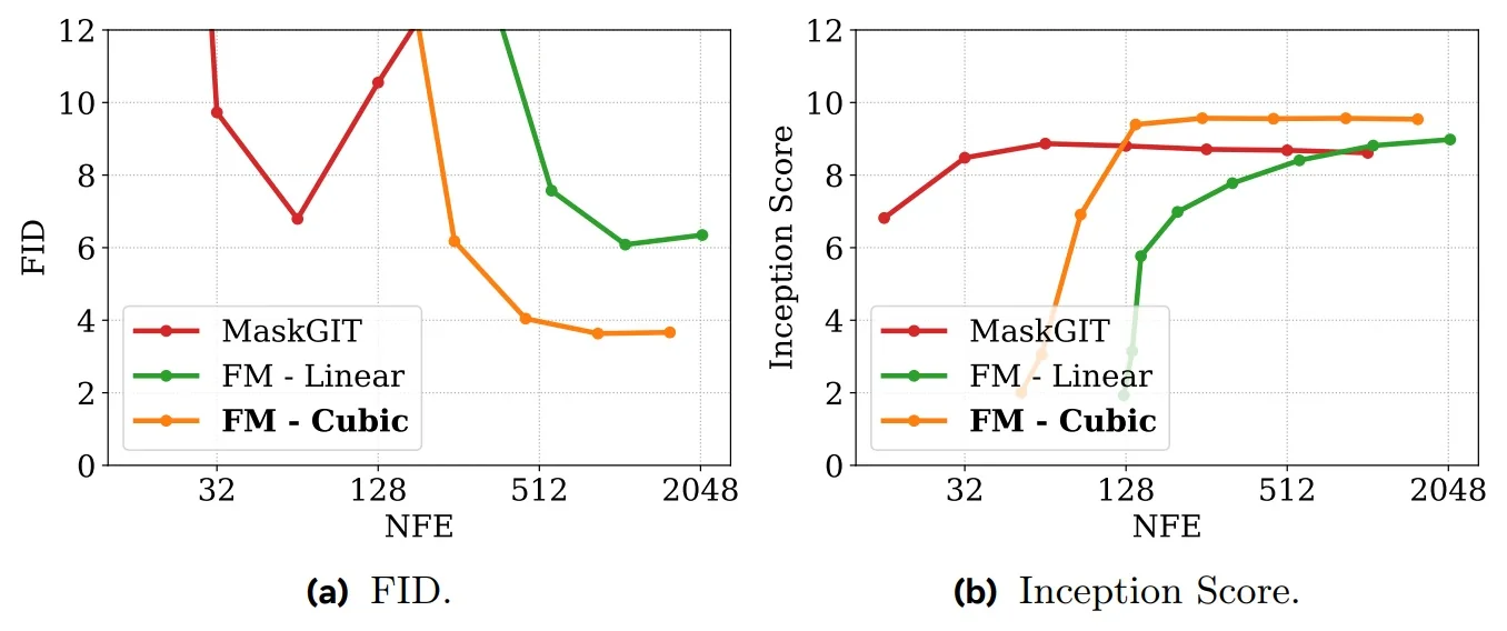
Beyond images, DFM emphasizes that CTMC flows are naturally compatible with non-left-to-right conditioning patterns. Figure 20.191 illustrates code generation where the model performs complex infilling (middle/right) rather than only prefix prompting (left), aligning with the bidirectional “fill missing parts” logic we exploited in MaskGIT, but now grounded in a continuous-time flow [171].
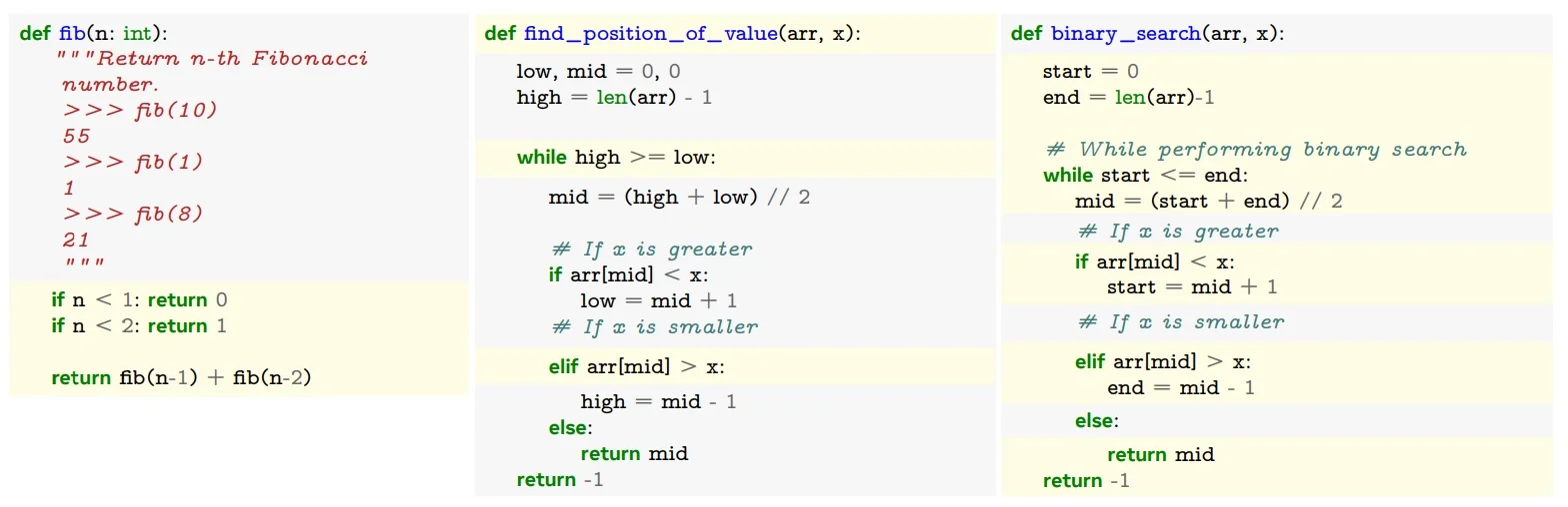
Ablations and Practical Lessons: Schedulers, Correctors, and “What Actually Matters” DFM’s ablations reinforce a pragmatic but important takeaway: in discrete flows, the probability path design (via \(\kappa _t\)) and the sampling strategy (forward-only vs. corrector) are not cosmetic details; they define the geometry of generation. In the image experiments, changing \(\kappa _t\) (e.g., linear vs. cubic) shifts the entire FID/IS–NFE curve (Figure 20.190). Corrector sampling via (20.172) provides a principled way to trade off diversity and refinement without reverting to MaskGIT-style confidence heuristics [171].
Limitations: What DFM Does Not Solve While DFM replaces heuristic unmasking with a principled CTMC dynamics, it does not eliminate iteration: sampling still requires multiple velocity evaluations (NFE) and careful scheduler design. Furthermore, the tractable constructions emphasized in DFM rely on token-wise path factorization (a scalability necessity), which can limit how richly the path itself captures cross-token dependencies; in practice, dependencies are learned through the denoiser network rather than being encoded directly in the path. Finally, CTMC simulation introduces discretization choices (step size, possible adaptive stepping, corrector coefficients) that can materially affect compute and quality.
Transition: From DFM to Generator Matching and Transition Matching DFM establishes that discrete-space generation can be framed as simulating a continuous-time Markov chain (CTMC) whose transition rates are derived from a learned denoiser. Having explored both continuous-space flows (standard FM) and discrete-space flows (DFM) operating in continuous time, the generative landscape appears mathematically fragmented: we rely on vector fields and ODEs for continuous data like images, but transition matrices and CTMCs for categorical data like text.
This fragmentation prompts two natural theoretical evolutions:
- A Unified Mathematical Framework: Can we construct a singular mathematical operator that unites all these continuous-time generative dynamics (ODEs, SDEs, and CTMCs) regardless of whether the underlying data type is continuous or discrete?
- Escaping Continuous Time: Can we subsequently abandon continuous time altogether to escape the computational bottleneck of sequential numerical solvers, allowing these models to scale natively within modern discrete-step autoregressive architectures?
Generator Matching [238] elegantly addresses the first question. Deriving bespoke probability paths and custom velocity formulas for every new data modality is mathematically cumbersome. Furthermore, generating hybrid multimodal data (e.g., interleaving continuous audio with discrete text tokens) is incredibly difficult when the modalities operate under fundamentally different physical equations. Rather than constructing velocities or rate matrices from specific probability paths, Generator Matching directly matches the infinitesimal generator of general Markov dynamics—the fundamental operator that dictates how probability evolves over continuous time in any space.
This provides a grand unification at the operator level. The practical gain is profound: continuous vector-field flows (ODEs), diffusion models (SDEs), and discrete jump processes (CTMCs) are entirely subsumed under a single mathematical objective. This enables seamless modeling of arbitrary and mixed state spaces without ever having to rewrite the underlying mathematical foundation.
Transition Matching [579] addresses the second question, marking a deliberate architectural departure to solve a critical inference bottleneck. While continuous-time dynamics are theoretically elegant, they are computationally expensive at inference. Simulating continuous time requires numerical ODE/SDE solvers or tiny CTMC step sizes (\(h \to 0\)) to accurately integrate the path, demanding a high Number of Function Evaluations (NFE). Transition Matching shifts the paradigm from continuous-time rates to discrete-time probability transitions. Why shift to discrete time? Because taking large, discrete, macroscopic jumps completely bypasses the need for iterative numerical solvers. By modeling discrete-time transitions (even over continuous states), we gain immense computational scalability. It allows the model to natively align with the causal, step-by-step processing pipelines that make modern Large Language Models (LLMs) so efficient. Ultimately, this framework provides the architectural bridge needed to unify flow-based continuous generation with highly optimized, large-scale autoregressive sequence modeling.
Enrichment 20.11.24: GM: Generator Matching
Motivation: A Universal Language for Continuous-Time Generation Flow Matching (FM) established an elegant recipe for continuous state spaces: define a tractable probability path from a simple prior to the data distribution, and learn the continuous dynamics—typically an ODE vector field—that transports probability mass along that path [373]. Discrete Flow Matching (DFM) successfully ported this principle to categorical domains, replacing vector fields with the probability velocities (transition rates) of a Continuous-Time Markov Chain (CTMC) [171]. Yet, this parallel evolution leaves the generative modeling landscape theoretically fragmented. Continuous flows, stochastic diffusions, and discrete jump processes are often treated as isolated mathematical families, forcing researchers to build bespoke, heavily engineered constructions when dealing with multimodal data (e.g., jointly generating continuous visual features and discrete text tokens).
Generator Matching (GM) [238] resolves this fragmentation by elevating the level of abstraction entirely. It grounds the generative problem in the fundamental observation that all modern step-wise generative models are Markov processes, and regardless of the underlying topology, every Markov process (under standard regularity conditions) is characterized by its infinitesimal generator, which determines the process’s local-in-time evolution and induces the corresponding distributional dynamics via the KFE.
What exactly is a generator? Intuitively, an infinitesimal generator is the mathematical “rulebook” that dictates exactly how a state will transition in the next infinitesimally small fraction of time. Instead of viewing continuous and discrete generative processes as fundamentally different, the generator framework reveals that they are simply different manifestations of this exact same operator:
- In an ODE (Flow Matching), the generator manifests as a vector field, dictating smooth, deterministic spatial movement.
- In a CTMC (Discrete Flow Matching), the generator manifests as a transition rate matrix, dictating the instantaneous probability of making a sudden categorical jump.
- In an SDE (Diffusion), the generator manifests as drift and diffusion coefficients, dictating continuous movement coupled with injected stochastic noise.
The core idea: Matching generators. If the generator is the rulebook, then training a generative model simply reduces to learning the correct rules to transform pure noise into the data distribution. Instead of designing bespoke loss functions for different modalities—such as Mean Squared Error for continuous vector fields or Cross-Entropy for discrete token distributions—GM proposes a single, universal training objective. The neural network predicts the parameters of the generator (whether continuous drift, diffusion variance, or discrete jump rates), and the loss function calculates the mathematical discrepancy between this predicted rulebook and the true rulebook required to stay on the target probability path. This is what it means to match generators.
By reframing generative modeling around this universal operator rather than highly specific, modality-dependent variables, GM yields a grand unification that unlocks capabilities previously thought to be theoretically incompatible:
-
Unifying continuous and discrete spaces. Historically, practitioners essentially had to learn two different fields: building a continuous diffusion model for images required stochastic differential equations (SDEs) and \(L_2\) losses, while building a discrete model for text required transition matrices and cross-entropy objectives. GM brings these under a shared mathematical umbrella. In practice, this means a single theoretical loss function (Generator Matching via Bregman divergence) trains both.
If you change your data from continuous pixels to discrete categorical tokens, you simply swap the generator operator in the math; the overarching training algorithm does not need a fundamental rewrite. An ODE flow and a categorical jump process are optimized using the exact same operator-level logic.
- Unlocking novel generative regimes: multiple KFE solutions for the same path. A key insight of GM is that fixing a probability path \(\{p_t\}\) does not uniquely determine the microscopic dynamics. Even for the same marginal evolution, the KFE can admit qualitatively different generators: smooth flows, stochastic diffusions, jump processes, and their superpositions. For continuous Euclidean data, prior work has focused almost exclusively on ODE flows and SDE diffusions. GM introduces Euclidean jump processes as a genuinely novel model class: samples can relocate discontinuously (“teleport”), matching the same marginal path without forcing all transport to be realized by continuous deformation. For certain paths (notably mixture-style), purely continuous flow solutions can become numerically stiff, demanding very large local velocities; jump processes provide a well-behaved alternative KFE solution [238]. GM also enables learning state-dependent diffusion coefficients \(\sigma _t(x)\) rather than fixing them as schedule-only functions, further expanding the design space.
- Principled model compositions via Markov Superpositions. Every generative process has geometric blind spots. Continuous flows are excellent at smooth, local pixel refinements (e.g., sharpening the edges of a face) but struggle with sharp discontinuous changes. Conversely, jump processes handle large structural shifts effortlessly but lack fine-grained local control. Because the underlying Kolmogorov Forward Equation is linear, GM proves we can simply add these generators together (\(\mathcal {L}_{\mathrm {total}} = \alpha _1 \mathcal {L}_{\mathrm {flow}} + \alpha _2 \mathcal {L}_{\mathrm {jump}}\)) on the exact same state space. During generation, an image sample can undergo a continuous deterministic drift to smooth its textures, while simultaneously experiencing stochastic, discrete jumps to radically alter its macro-structure. The model gets the best of both worlds, leading to demonstrably superior generation quality (such as lower FID scores).
-
Tractable multimodal generation. Generating continuous images and discrete text simultaneously is traditionally hindered by the “curse of dimensionality”. Attempting to define a single, joint mathematical rulebook across both domains (e.g., mapping every possible pixel combination against every possible vocabulary word) is computationally impossible.
GM bypasses this roadblock by showing that with a factorized conditional path (independent across modalities given \(z=(z_1,z_2)\)), the conditional generator admits an additive coordinate-wise decomposition. This avoids an exponentially large joint transition object while still allowing cross-modal dependence to enter through the shared network input \(x=(x^{(1)},x^{(2)})\). In practice, we can evolve the continuous image via an ODE/SDE component and the discrete text via a CTMC component side-by-side.
Because the network “sees” both domains simultaneously at every time step, the image and text dynamically condition and align with one another as they collaboratively emerge from the noise. This preserves true multimodal coherence while entirely avoiding an exponential blowup in network parameters [238].
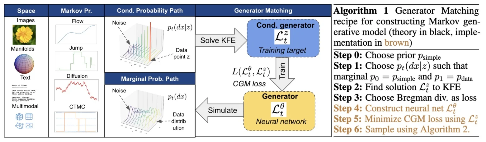
Road map. The GM framework builds a universal generative model through a logical sequence of five steps. Here is how we will navigate the theory:
- 1.
- Probability paths (The Blueprint): Before we figure out how to move probability mass, we must decide where we want it to go. We start by defining a conditional probability path \(p_t(\mathrm {d}x\mid z)\). This is a simple, closed-form trajectory that describes how pure noise smoothly morphs into a single, specific data point \(z\) (e.g., a specific image of a cat). By averaging these simple conditional paths over every data point in our training set, we implicitly define the marginal probability path \(p_t\)—the highly complex, global trajectory that transforms the entire noise distribution into the full data distribution.
- 2.
- Generators and the KFE (The Physics): Once the path is drawn, we need the physics engine to traverse it. We define the infinitesimal generator \(\mathcal {L}_t\), which acts as the mathematical “rulebook” for how a single state transitions at any given micro-instant (e.g., how much to drift, how much noise to add, or whether to make a sudden discrete jump). We then establish the Kolmogorov Forward Equation (KFE). The KFE is the master conservation law connecting the micro to the macro: it proves that if all individual states follow the local rules of \(\mathcal {L}_t\), the global probability cloud will correctly evolve along our chosen path \(p_t\) over time.
- 3.
- Marginalization (The Conditional-to-Marginal Trick): Finding the true marginal generator (the global rulebook required to generate the entire dataset) is analytically impossible because the data distribution is too complex. However, finding the conditional generator (the rulebook to generate just one specific target image \(z\)) is trivial. GM proves a crucial bridging theorem: the intractable marginal generator is exactly equal to the posterior expectation of the simple conditional generators. In plain terms, the complex global rules are just a weighted average of the simple local rules.
- 4.
- Training via CGM (The Tractable Objective): We introduce
the Conditional Generator Matching (CGM) loss to train our
neural network. Because calculating the true marginal generator is
computationally impossible, we instead train the network to constantly
guess the simple, conditional generators. The magic here relies
on Bregman divergences—a strict family of geometric distance
functions.
Because Bregman divergences interact perfectly with expectations, measuring the loss against the simple conditional targets mathematically guarantees that the network’s gradients are well aligned with the ideal, intractable marginal objective. The network implicitly learns the global rules by explicitly practicing on the local ones.
- 5.
- Markov Compositions (The Practical Payoff): Finally, we reap the architectural benefits of this operator-level theory. Because the KFE is a strictly linear equation, we can exploit it to build advanced models that were previously impossible. We explore Markov Superpositions, where we literally add different generators together (e.g., blending a continuous flow ODE with a discrete CTMC jump process on the exact same image space) to cover each other’s geometric blind spots. We also explore Multimodal Models, showing how independent generators (one for text, one for images) can be seamlessly coupled into a joint product space without suffering an exponential blowup in parameters.
Probability Paths: Conditional Design, Marginal Consequence To generate data, we need a roadmap that guides probability mass from a simple, easy-to-sample prior distribution (like pure noise) to the highly complex target data distribution. However, attempting to design this massive, global transformation all at once is mathematically overwhelming.
GM solves this using a “divide and conquer” strategy. We design the path locally for a single data point, and the global path emerges naturally as a consequence. Let \(\mathcal {S}\) be an arbitrary state space (this could be continuous pixels, discrete text tokens, or a complex multimodal combination). The framework operates in two distinct phases:
- The Conditional Path (The Local Roadmap): Instead of looking at the whole dataset, we anchor our focus on a single, specific data point \(z\) drawn from our dataset \(p_{\mathrm {data}}\) (e.g., one specific image of a dog). We define a conditional probability path \(\{p_t(\mathrm {d}x\mid z)\}_{t\in [0,1]}\). This path dictates exactly how pure noise (\(p_{\mathrm {simple}}\) at \(t=0\)) smoothly transitions into that single target data point (a Dirac delta \(\delta _z\) at \(t=1\)).
- The Marginal Path (The Global Roadmap): Once we have the simple rules for how noise reaches any individual point \(z\), we find the global path by simply averaging all these individual paths together, weighted by the real data distribution. Marginalizing over \(z\) induces the overarching marginal path: \begin {equation} p_t(\mathrm {d}x) \;=\; \int p_t(\mathrm {d}x\mid z)\,p_{\mathrm {data}}(\mathrm {d}z) \label {eq:chapter20_gm_marginal_path} \end {equation} With this target marginal path mathematically defined, the entire generative modeling problem reduces to a single task: find a Markov process whose probability evolution perfectly matches \(\{p_t\}\).
The Two Canonical Path Families
How exactly does noise turn into the target \(z\)? The choice of the conditional path completely changes the geometric nature of the generation. GM emphasizes two canonical families that represent fundamentally different ways to travel through state space:
-
Mixture paths (Probabilistic Teleportation): \begin {equation} p_t(\mathrm {d}x\mid z) = (1-\kappa _t)\,p_{\mathrm {simple}}(\mathrm {d}x) + \kappa _t\,\delta _z(\mathrm {d}x), \qquad \kappa _0=0,\;\kappa _1=1. \label {eq:chapter20_gm_mixture_path} \end {equation} Intuition: This path performs a probability “cross-fade”. At any intermediate time \(t\), the state does not physically morph into a half-noise/half-data hybrid.
Instead, it is strictly either pure noise (with probability \(1-\kappa _t\)) or it has instantaneously “teleported” to the exact target \(z\) (with probability \(\kappa _t\)). In continuous Euclidean settings, the endpoint Dirac \(\delta _z\) is typically mollified to a narrow kernel (e.g., \(\mathcal {N}(z,\sigma _{\min }^2 I)\)) for numerical stability, but the conceptual behavior is unchanged [238]. Because mixture paths do not require intermediate fractional states, they apply on arbitrary state spaces \(\mathcal {S}\), making them particularly natural for discrete domains (text, graphs, categorical structures).
- Geometric averages (Euclidean morphing): \begin {equation} X_t = \sigma _t X_0 + \alpha _t z, \qquad X_0\sim p_{\mathrm {simple}},\;\; \alpha _0=\sigma _1=0,\;\alpha _1=\sigma _0=1, \label {eq:chapter20_gm_geomavg_path} \end {equation} Intuition: Unlike mixture paths, this family mixes states rather than probabilities. The sample \(X_t\) is a physical, continuous blend of the noise \(X_0\) and the target \(z\). As \(t\) progresses, the noise fades out (\(\sigma _t \to 0\)) while the target structure fades in (\(\alpha _t \to 1\)). This straight-line Euclidean interpolation is closely related to the conditional optimal transport (CondOT) paths used in continuous Flow Matching [238]. Because it requires intermediate fractional states, a vector-space structure (\(\mathcal {S}\subseteq \mathbb {R}^d\)) is necessary, making this family the natural choice for images, audio, and video.
Generators: The Engine of Probability Transport We have just established our “roadmaps”—the probability paths \(\{p_t\}\) that dictate how the overall distribution should evolve, whether through discrete probabilistic teleportation or continuous geometric morphing. However, a roadmap does not move the data; we need an engine.
In GM, the engine that physically transports a state along the path is a time-continuous Markov process \(\{X_t\}_{t\in [0,1]}\). Rather than looking at discrete, macroscopic steps of this process, we analyze its instantaneous behavior. We ask: at this exact micro-second, what is the rule for how the state \(X_t\) will change? This local rule is formalized by the infinitesimal generator, denoted \(\mathcal {L}_t\).
Mathematically, for any well-behaved test function \(f\) (which you can think of as a physical measurement of the state), the generator measures the expected rate of change: \begin {equation} [\mathcal {L}_t f](x) \;=\; \lim _{h\to 0}\frac {\mathbb {E}[f(X_{t+h})\mid X_t=x]-f(x)}{h} \label {eq:chapter20_gm_generator_def} \end {equation}
Generators in Practice. The elegance of the generator is that it translates directly into the physical transportation methods we designed in our paths. Depending on how we parameterize \(\mathcal {L}_t\), we recover the exact engines used in modern generative models:
- Flows (Continuous steering): \(\mathcal {L}_t f(x)=\nabla f(x)^\top u_t(x)\). Here, the generator is simply a vector field \(u_t(x)\). It acts as a deterministic steering wheel, perfectly suited for driving samples along the continuous morphing (geometric average) paths.
- Diffusions (Steering with noise): \(\mathcal {L}_t f(x)=\nabla f(x)^\top u_t(x)+\tfrac {1}{2}\,\mathrm {Tr}\!\big (\sigma _t^2(x)\,\nabla ^2 f(x)\big )\), where \(\sigma _t^2(x)\succeq 0\) is the instantaneous diffusion (covariance) matrix. The generator still contains a drift \(u_t\) for continuous steering, but also injects state-dependent noise, spreading probability mass while evolving along the target path [238].
- Jump processes (Probabilistic teleportation): \(\mathcal {L}_t f(x)=\int (f(y)-f(x))\,Q_t(\mathrm {d}y; x)\). Here, there is no continuous spatial derivative. Instead, the generator uses a rate matrix \(Q_t\) to define sudden, discontinuous jumps from state \(x\) to state \(y\). This is the exact engine required to execute the mixture paths on discrete data like text.
The Master Conservation Law: The Kolmogorov Forward Equation (KFE) If the generator \(\mathcal {L}_t\) acts as the local steering rule for individual particles, how do we guarantee that the macroscopic cloud of all particles successfully follows our global roadmap \(p_t\)?
They are linked by a fundamental law of physics and probability called the Kolmogorov Forward Equation (KFE). The KFE acts as a strict conservation law, demanding that the global change in the probability distribution perfectly balances the net movement generated by our local rules:
\begin {equation} \frac {\mathrm {d}}{\mathrm {d}t}\,\langle p_t, f\rangle \;=\; \langle p_t, \mathcal {L}_t f\rangle , \qquad \forall f\in \mathcal {T} \label {eq:chapter20_gm_kfe} \end {equation} (where the bracket notation \(\langle p_t,f\rangle := \int f(x)\,p_t(\mathrm {d}x)\) simply means the expected value of \(f\) over the distribution \(p_t\)).
Why is the KFE the centerpiece of GM? The KFE bridges our design phase with our training phase, yielding two profound takeaways for generative modeling:
- It defines the ultimate objective. The entire GM paradigm can be summarized in one sentence: Design a target probability path \(\{p_t\}\), then train a neural network to predict a generator \(\mathcal {L}_t\) that mathematically balances the KFE for that path. In the idealized limit of an exact generator and exact simulation, satisfying the KFE implies the marginal law of \(X_t\) follows the designed path \(p_t\) and reaches \(p_1=p_{\mathrm {data}}\). In practice, numerical discretization and approximation error mean we only match this behavior approximately.
- It enables principled model combinations. Crucially, the KFE is strictly linear with respect to the generator \(\mathcal {L}_t\). If you have a valid flow generator and a valid jump generator that both solve the KFE, any affine combination of the two also solves it. This linearity is the mathematical foundation that allows us to safely superimpose completely different generative processes onto the same state space without breaking the model.
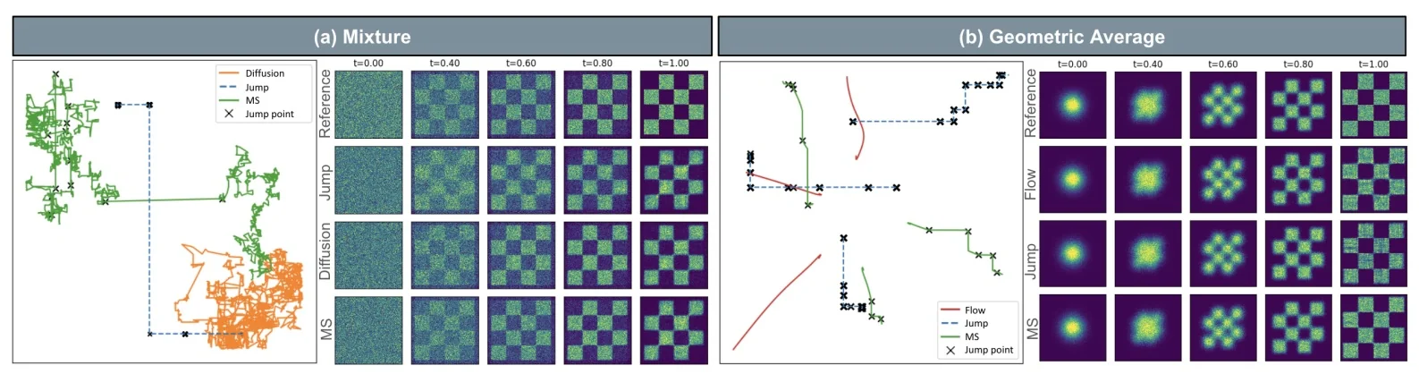
The Marginalization Trick: Posterior Averaging of Generators We now know that we need to find the marginal generator \(\mathcal {L}_t\) that dictates the global evolution of the probability distribution. However, directly solving for this global operator is mathematically intractable because it depends on the complex, unknown structure of the entire dataset \(p_{\mathrm {data}}\).
To solve this, GM utilizes a conditional-to-marginal trick. We drop the global perspective and instead ask a local question: what is the generator \(\mathcal {L}_t^z\) required to drive noise toward just a single, known data point \(z\)? Because the conditional path to a single point is simple (e.g., straight-line morphing or simple probabilistic teleportation), calculating its conditional KFE solution \(\mathcal {L}_t^z\) is trivial.
The central structural result of GM proves that the complex marginal generator is exactly equal to the posterior average of these simple conditional generators: \begin {equation} [\mathcal {L}_t f](x) \;=\; \mathbb {E}_{z\sim p_{1\mid t}(\cdot \mid x)}\!\left [[\mathcal {L}_t^{z} f](x)\right ] \label {eq:chapter20_gm_posterior_avg} \end {equation} Intuition: If you observe a noisy state \(x\) at time \(t\), you do not know exactly which clean image \(z\) it will eventually become. The posterior \(p_{1\mid t}(\mathrm {d}z\mid x)\) represents your mathematical belief over all possible true endpoints. Equation 20.179 states that the true global rulebook (\(\mathcal {L}_t\)) is simply a weighted average of all the local rulebooks (\(\mathcal {L}_t^z\)), weighted by how likely it is that \(x\) is heading toward \(z\).
Moreover, when the conditional generators admit a linear parameterization by concrete coefficients \(F_t^z(x)\) (e.g., drift fields, diffusion matrices, or jump-rate parameters), the marginal coefficients are simply the posterior expectation: \begin {equation} F_t(x) \;=\; \mathbb {E}_{z\sim p_{1\mid t}(\cdot \mid x)}\!\big [F_t^{z}(x)\big ] \label {eq:chapter20_gm_param_posterior_avg} \end {equation} This parameter-level identity is the key bridge that makes conditional training targets sufficient for learning the intractable marginal dynamics [238].
Training via Conditional Generator Matching (CGM) We now have the true target (\(\mathcal {L}_t\)), and we want to train a neural network to parameterize our learned generator, \(\mathcal {L}_t^\theta \). Let \(F_t(x)\) denote the concrete parameters of the generator at time \(t\) (e.g., the continuous drift velocity \(u_t(x)\), the diffusion variance \(\sigma _t^2(x)\), or the discrete jump rate matrix \(Q_t(\cdot ;x)\)). Our neural network predicts these parameters as \(F_t^\theta (x)\).
Step 1: The Ideal (but Impossible) Objective. The most direct way to train the network would be to measure the distance between its prediction \(F_t^\theta (x)\) and the true marginal parameters \(F_t(x)\) along the probability path: \[ \mathbb {E}_{t\sim \mathcal {U}(0,1)}\,\mathbb {E}_{x\sim p_t}\big [D_\phi \big (F_t(x),F_t^\theta (x)\big )\big ] \] Here, \(D_\phi \) represents a Bregman divergence—a broad class of distance metrics generated by a strictly convex function \(\phi \) (Mean Squared Error and KL-divergence are both special cases of Bregman divergences). However, we cannot compute this loss because we do not analytically know the marginal target \(F_t(x)\).
Step 2: Why Bregman divergences are essential. GM does not claim that an arbitrary loss allows replacing the marginal target by conditional targets. The key requirement is that \(D_\phi \) is a Bregman divergence, and GM proves this condition is both sufficient and essentially necessary. Under this assumption, the ideal but intractable marginal Generator Matching objective and the Conditional Generator Matching (CGM) objective differ only by a constant independent of \(\theta \). Equivalently, their gradients coincide: \[ \nabla _\theta \mathcal {L}_{\mathrm {GM}}(\theta ) \;=\; \nabla _\theta \mathcal {L}_{\mathrm {CGM}}(\theta ), \] so optimizing CGM yields the same learning signal as the marginal objective, without ever needing to compute the marginal generator explicitly [238].
Step 3: The Tractable CGM Loss. We can therefore replace the unknown marginal target \(F_t(x)\) with the computable conditional target \(F_t^{z}(x)\), yielding the highly scalable Conditional Generator Matching (CGM) loss:
\begin {equation} \mathcal {L}_{\mathrm {CGM}}(\theta ) = \mathbb {E}_{t\sim \mathcal {U}(0,1)} \mathbb {E}_{z\sim p_{\mathrm {data}}} \mathbb {E}_{x\sim p_t(\cdot \mid z)} \Big [ D_\phi \!\big (F_t^{z}(x),\,F_t^\theta (x)\big ) \Big ] \label {eq:chapter20_gm_cgm} \end {equation}
Intuition: During training, you do not need to simulate the complex global dynamics or calculate the posterior. You simply:
- 1.
- Sample a real data point \(z\) and a random time \(t\).
- 2.
- Add noise to \(z\) according to the simple conditional path to get state \(x\).
- 3.
- Calculate the known conditional rulebook \(F_t^z(x)\) for that specific sample.
- 4.
- Penalize the neural network’s prediction \(F_t^\theta (x)\) against this simple target using a Bregman divergence.
Because of the underlying Bregman geometry, optimizing this simple, single-sample loss mathematically guarantees that the network is implicitly learning the complex, dataset-wide marginal generator.
# Generator Matching (conceptual CGM training loop).
# Choose conditional path p_t(dx|z); sample t, z, x~p_t(.|z); compute conditional target F_t^z(x);
# minimize Bregman divergence D_phi(F_t^z(x), F_t^theta(x)).

for step in range(num_steps):
    t = uniform(0.0, 1.0)
    z = sample_data()
    x = sample_conditional_path(t, z)     # x ~ p_t(. | z)
    target = conditional_generator_params(t, x, z)   # F_t^z(x), closed-form for chosen path family
    pred = net_generator_params(theta, t, x)       # F_t^theta(x)
    loss = bregman_divergence(target, pred)
    loss.backward()
    optimizer.step()
Markov Superpositions: The Best of Both Worlds Every generative engine has inherent geometric strengths and blind spots. Continuous flows (ODEs) are excellent at smooth, local refinements—such as subtly adjusting the color gradient of a pixel—but they struggle immensely when forced to execute sharp, discontinuous topological changes. Conversely, jump processes (CTMCs) can effortlessly execute massive structural leaps by instantaneously teleporting a state, but they are entirely incapable of making fine, continuous local adjustments.
What if we want the local finesse of a flow and the global flexibility of a jump process in the exact same model?
Because GM is grounded in the Kolmogorov Forward Equation (KFE), the solution is surprisingly simple. The KFE, which governs how the probability distribution evolves, is a strictly linear equation. This linearity guarantees a profound mathematical property: any affine combination of generators that individually solve the KFE for a specific path will also perfectly solve the KFE for that exact same path.
The Superposition Equation. Suppose we have already found two valid generators that independently hit our target marginal path \(\{p_t\}\): a continuous flow generator \(\mathcal {L}_t^{(1)}\) and a discrete jump generator \(\mathcal {L}_t^{(2)}\). We can construct a Markov Superposition by simply taking their weighted average:
\begin {equation} \mathcal {L}_t^{\mathrm {MS}} \;=\; \alpha _1(t)\,\mathcal {L}_t^{(1)} + \alpha _2(t)\,\mathcal {L}_t^{(2)}, \qquad \alpha _1(t),\alpha _2(t)\ge 0,\;\;\alpha _1(t)+\alpha _2(t)=1, \label {eq:chapter20_gm_superposition} \end {equation}
For any valid choice of time-varying weights \(\alpha _1(t),\alpha _2(t)\), the resulting superposed process still perfectly hits the target data distribution at \(t=1\), just as reliably as either standalone model.
Physical Interpretation and Practical Gains. Operationally, the superposition \(\mathcal {L}_t^{\mathrm {MS}}\) corresponds to running multiple Markov mechanisms on the same state in continuous time. For a flow+jump superposition, the state evolves with a continuous drift component at all times, while jump events occur at random times governed by the jump generator’s rate kernel. In a discrete-time numerical implementation this often manifests as predominantly flow-like updates punctuated by occasional stochastic jump moves, but the underlying interpretation is a single unified Markov process whose infinitesimal rule is given by Equation 20.182 [238].
This is not just a theoretical curiosity; it yields tangible improvements. Empirically, the paper shows that superpositions (e.g., flow+jump) can outperform the corresponding pure components in sample quality. One useful intuition is that the jump component enables occasional nonlocal moves, complementing the flow’s local refinement behavior [238].
Multimodal Product Spaces: Taming the Curse of Dimensionality Consider the challenge of generating an image and its descriptive text simultaneously. Mathematically, this requires defining a generative process over a joint product space: \(\mathcal {S} = \mathcal {S}_1 \times \mathcal {S}_2\) (where \(\mathcal {S}_1\) is the continuous pixel space and \(\mathcal {S}_2\) is the discrete vocabulary space).
Traditionally, this is a mathematical nightmare. Constructing a joint transition operator across a product space causes an exponential blowup in parameters—the model would theoretically need to calculate the transition probability of every possible pixel combination against every possible vocabulary word. GM sidesteps this curse of dimensionality entirely through a brilliant mathematical property of the conditional KFE.
The Multimodal Factorization Trick. The solution relies on how we design the target probability path. If we define the joint conditional probability path so that it factorizes (meaning the image noise path and the text noise path are independent given the final target \(z = (z_1, z_2)\)), a cascade of mathematical simplifications occurs:
- Additive conditional generators. Because the conditional probability path factorizes (\(p_t(\mathrm {d}x \mid z) = p_t(\mathrm {d}x_1 \mid z_1) p_t(\mathrm {d}x_2 \mid z_2)\)), solving the Kolmogorov Forward Equation becomes trivial. The joint conditional KFE perfectly splits into two independent equations. Consequently, the joint conditional generator decomposes in the standard “sum of coordinate generators” form: for any test function \(f(x_1,x_2)\), \[ [\mathcal {L}_t^{z} f](x_1,x_2) = [(\mathcal {L}_{t,1}^{z_1} f(\cdot ,x_2))](x_1) + [(\mathcal {L}_{t,2}^{z_2} f(x_1,\cdot ))](x_2). \] Intuitively: one generator updates the image-coordinate while treating the text-coordinate as fixed, and the other updates the text-coordinate while treating the image-coordinate as fixed [238].
- Additive loss functions. For separable generator parameterizations and separable Bregman divergences (i.e., \(\phi =\phi _1+\phi _2\)), the joint CGM objective decomposes into a sum of unimodal losses: \(\mathcal {L}_{\mathrm {total}}=\mathcal {L}_{\mathrm {CGM}}^{(1)}+\mathcal {L}_{\mathrm {CGM}}^{(2)}\). Operationally, this corresponds to combining a continuous loss (e.g., MSE-style for flow/diffusion parameters) with a discrete loss (e.g., KL/CE-style for jump-rate parameters).
-
Cross-modal conditioning (The “glue”). If the math is completely split, how do the text and image actually relate to each other? The magic happens in the neural network architecture. While the target math is independent, the neural network predicting the generator parameters at time \(t\) takes the entire joint noisy state \(x = (x^{(1)}, x^{(2)})\) as its input.
When predicting the next update for the image, the network looks at the currently noisy text; when predicting the next update for the text, it looks at the currently noisy image. Because the network constantly shares this context across modalities at every infinitesimal time step, the two modalities dynamically guide, condition, and align with each other as they collaboratively emerge from the noise.
By proving that additive generators and additive losses are mathematically rigorous under the KFE, GM provides a principled, highly scalable route to true multimodal generative models without ever requiring an exponentially large joint transition object [238].
Limitations: The Bottleneck of Continuous Time Generator Matching provides a beautiful, mathematically unified theory for generative modeling, but it remains fundamentally constrained by one harsh practical reality: it operates entirely in continuous time.
To actually generate an image or a sequence using an infinitesimal generator, we must simulate the continuous process using numerical integration (e.g., Euler ODE/SDE solvers or Gillespie CTMC algorithms). This requires chopping the generation trajectory into dozens or hundreds of tiny, sequential fractions. Every single micro-step demands a full forward pass of a massive neural network (resulting in a high Number of Function Evaluations, or NFE), making inference computationally expensive and inherently slow.
Furthermore, GM still relies heavily on human design. The marginalization trick only works if we can analytically solve the conditional KFE. This restricts researchers to manually hand-crafting simple, mathematically convenient “roadmaps” (conditional paths) rather than allowing the model to freely learn the most optimal, data-driven route.
Transition: From Micro-Steps to Macro-Leaps We have pushed continuous-time generation to its theoretical ceiling. To truly scale these paradigms to the magnitude of modern foundation models, we must eliminate the reliance on slow, fine-grained numerical solvers. We need models that do not inch forward, but rather take massive, confident strides.
If GM represents the ultimate unification of infinitesimal, continuous-time rules, the next logical evolution is to unify finite, discrete-time rules. Transition Matching (TM) [579] achieves exactly this.
TM completely abandons the continuous generator, shifting the mathematical focus to learning arbitrary, large-step discrete transitions over continuous state spaces. By mapping massive leaps through space rather than integrating micro-steps, TM perfectly bridges the continuous geometric flexibility of Flow/Diffusion models with the raw, highly scalable, “next-step” computational efficiency of modern Autoregressive (LLM-style) architectures.
Enrichment 20.11.25: TM: Transition Matching
Motivation: Escaping the Continuous-Time Bottleneck Flow Matching (FM) provides an elegant recipe for generative modeling in continuous state spaces: specify a tractable probability path and learn an infinitesimal velocity field whose induced Ordinary Differential Equation (ODE) transports mass from pure noise to the data manifold [373]. Discrete Flow Matching (DFM) extended this exact continuous-time formulation to discrete categorical domains by replacing vector fields with the transition rates of a Continuous-Time Markov Chain (CTMC) [171]. Generator Matching (GM) subsequently elevated this viewpoint into a grand unification, proving that continuous flows, stochastic diffusions, and discrete jump processes are all mathematically united as continuous-time Markov processes characterized by their infinitesimal generators [238].
However, this beautiful continuous-time unification imposes a severe computational tax during inference. Because the learned operator in FM, DFM, and GM is strictly infinitesimal (dictating movement for only a microscopic fraction of time), generating a single sample fundamentally requires numerical integration. Simulating these ODE, SDE, or CTMC solvers forces the model to inch forward through dozens or hundreds of sequential micro-steps. If a practitioner attempts to accelerate generation by taking massive discrete steps, the linear tangent approximations of the numerical solver wildly diverge from the true curved probability path, yielding severe discretization artifacts.
The Architectural Divide. Concurrently, the broader artificial intelligence ecosystem is heavily dominated by Autoregressive (AR) sequence models, such as Large Language Models. These architectures are natively built for discrete-time, causal generation, aggressively leveraging hardware-accelerated mechanisms like KV-caching to scale to massive parameter counts. Yet, forcing continuous visual data into these discrete AR frameworks traditionally requires lossy tokenization via Vector Quantized Variational Autoencoders (VQ-VAEs), artificially grouping continuous pixels into discrete categorical vocabularies and discarding fine-grained structural fidelity.
Transition Matching (TM) [579] introduces a deliberate structural paradigm shift designed to synthesize the best of both domains and complete the generative modeling matrix: keep the state space strictly continuous, but discretize time to learn finite Markov transitions.
Rather than learning an infinitesimal generator to power a continuous solver (as in GM), TM explicitly trains the neural network to predict the exact probability distribution of massive, discrete leaps through space. What TM brings to the table is profound:
- It preserves the artifact-free, high-fidelity geometry of continuous latent spaces found in diffusion and FM.
- It eliminates the need for continuous-time ODE/SDE solvers and therefore removes numerical integration discretization error, enabling high-quality generation in very few steps (with the remaining approximation coming from the learned finite-step kernels and the chosen step count).
- It naturally aligns continuous geometric data with the discrete-time, next-step causal mechanics of modern AR architectures, unlocking LLM-style scaling for continuous features without relying on VQ-VAE tokenization.
By explicitly training the network to predict the exact probability distribution of massive, discrete leaps through space—rather than predicting continuous, instantaneous velocities—TM achieves several critical breakthroughs:
- Elimination of discretization error: In standard continuous-time models, the neural network predicts an instantaneous derivative (a tangent vector). When an ODE solver attempts to take a large discrete step along this linear tangent, it inevitably diverges from the true, curved probability path. This structural error forces practitioners to use dozens of computationally expensive micro-steps to keep the generation trajectory on track. TM bypasses this entirely by learning the exact finite difference between states (a true secant vector, formalized as the “Difference Latent”). Because the model explicitly predicts the finite displacement required to sample a valid next state under the target transition kernel at \(t+1\), it is mathematically aware of its discrete step size. This natively enables high-quality generation in very few steps (e.g., 4 to 8 steps) without drifting off the underlying data manifold.
-
Token-free continuous geometry: Traditional attempts to apply Autoregressive models to visual data rely on Vector Quantized Variational Autoencoders (VQ-VAEs) to artificially discretize the continuous visual world. This inherently lossy compression forces smooth pixel features into a rigid, finite vocabulary of discrete tokens, frequently resulting in quantization artifacts, jagged edges, and the loss of high-frequency textures. In contrast, TM operates directly on unquantized, continuous latent features in \(\mathbb {R}^d\).
This preserves the exact, high-fidelity spatial geometry and smooth gradients native to diffusion models, entirely circumventing the information bottleneck of categorical tokenization.
- Autoregressive architectural synergy: By discretizing time into sequential steps \(X_0, X_1, \dots , X_T\) while keeping the state space continuous, TM bridges the architectural divide. The continuous states \(X_t\) act as unquantized “embeddings” that can be processed sequentially. This maps the generative process perfectly onto the causal sequence modeling framework that drives modern foundation model scaling. It allows continuous data to be generated autoregressively using unmodified causal Transformer architectures, seamlessly unlocking standard LLM hardware efficiencies—most notably KV-caching, which allows the model to attend to the full continuous generation history without redundant recomputations [350, 154].
Which Variant is “Best”? Observing the qualitative improvements in Figure 20.194, a natural engineering question arises: is FHTM the ultimate goal, or is DTM the more practical choice? The answer depends entirely on the desired architectural foundation. Neither model is universally “better” than the other; rather, they solve two different infrastructural bottlenecks by making distinct choices along Axis 3 (the Kernel Modeling Paradigm).
-
DTM (The Practical Drop-In Upgrade): DTM is highly practical. By enforcing a strict Markovian constraint (where the transition depends solely on the current state \(X_t\)), DTM acts as a direct, drop-in mathematical replacement for standard continuous-time Flow Matching. It seamlessly integrates into existing U-Net and DiT pipelines. DTM is the optimal choice when the goal is to upgrade an established diffusion/flow architecture to natively support massive, artifact-free discrete leaps, thereby drastically improving few-step generation quality without overhauling the underlying network structure.
- FHTM (The Autoregressive Frontier): FHTM is an ambitious architectural bridge. By adopting a fully causal paradigm (where the transition depends on the entire continuous sequence history \(X_{0:t}\)), FHTM trades the simplicity of a Markov chain for the scaling mechanics of a Large Language Model. It is the ideal choice when building unified, multimodal foundation models. Because FHTM treats continuous visual features exactly like a sequence of text tokens, it allows unmodified causal Transformers to generate continuous images autoregressively, fully exploiting hardware-level LLM optimizations like KV-caching.
Bridging the Theory. In the following sections, we will rigorously demonstrate how both models work from the ground up. We will first establish the shared mathematical foundation required to teach a network how to execute discrete jumps, locking in our choices for the supervising process (Axis 1) and the difference latent parameterization (Axis 2). Once the core discrete-time objective is derived, we will explicitly show how varying the context window on Axis 3 mathematically branches the framework into the practical DTM and the autoregressive FHTM.
Road map: The Three-Axis Design Space To intuitively understand Transition Matching, imagine you are trying to cross a river. Continuous Flow Matching (FM) assumes you are being carried by a smooth, continuous current (an ODE), where your exact position is defined at every microsecond. Transition Matching abandons the current. Instead, it treats crossing the river as a sequence of discrete, massive jumps across a finite set of stepping stones.
Because we are no longer bound by the rigid physics of a continuous current, we have the freedom to design this jumping process from scratch. TM organizes this freedom into a modular, highly expressive three-axis design space.
Building a TM model requires making one choice along each axis:
-
Axis 1: The Supervising Process (Defining the Stepping Stones). Before the model can learn to jump, we must define the valid landing zones. This axis determines how we construct the ground-truth training paths from pure noise to real data. Instead of assuming a continuous physical flow governed by an ODE, we define a discrete, finite sequence of intermediate states \(\{X_0, X_1, \dots , X_T\}\).
A crucial note on notation: If you are accustomed to standard diffusion literature, you are likely used to \(X_T\) representing pure noise and \(X_0\) representing the clean data. Transition Matching (following the Flow Matching convention) reverses this index to align with the forward generative direction of time. Here, \(X_0\) is the starting point (pure, unstructured noise). As the step index \(t\) increases, the state becomes progressively clearer, accumulating structure until it perfectly lands on the target data manifold at \(X_T\).
The supervising process dictates the exact geometric location of these intermediate stones. Because time is discrete, these stepping stones do not have to be infinitesimally close together; we can mathematically design them to support massive, abrupt leaps through the state space toward clarity.
-
Axis 2: The Kernel Parameterization (Defining the Jump Instruction). Once the stones are placed, what exact mathematical instruction should the neural network output to successfully jump from a noisy state \(X_t\) to the slightly cleaner state \(X_{t+1}\)?
-
Targeting absolute coordinates (predicting the full clean target \(X_{t+1}\) directly) is notoriously unstable and prone to averaging out fine details in high dimensions.
- Targeting velocity (predicting an instantaneous tangent vector, as in FM) is mathematically dangerous for large discrete jumps; if you simply ”face north and walk” for too long without recalculating, the linear tangent will deviate from the curved probability path, causing you to miss the next stone entirely.
-
Targeting the difference (predicting \(Y = X_{t+1} - X_t\)) is the TM solution. At a high level, this operates on the proven principle of residual learning: instead of forcing the network to predict the absolute coordinates of an entire complex image from scratch, it only needs to predict the specific structural updates required for the current step. More importantly, the network regresses a latent target representing the exact finite displacement vector (a true “secant” jump).
In continuous Flow Matching, the network predicts an instantaneous tangent velocity. If an ODE solver attempts to take a large discrete step using this straight tangent line, it inherently overshoots the true curved probability path. This is the root of discretization error, which typically forces continuous models to use dozens of tiny micro-steps to stay on track. By predicting the finite difference, the TM model learns to sample a valid next state under the target transition kernel at \(t+1\). It absorbs the discrete step size directly into its prediction, thereby avoiding the ODE solver discretization error that arises from scaling an infinitesimal tangent field to large step sizes.
The Inference Step-Count Trade-off. A natural question arises: doesn’t explicitly learning the specific jump \(X_{t+1} - X_t\) lock the model into using the exact same number of steps (\(N\)) during inference as it saw during training?
Generally, yes. A discrete-time Markov chain trained on a specific sequence of stepping stones expects to traverse those exact stones during generation.
While this admittedly sacrifices the arbitrary-time continuous querying flexibility of an ODE, it transforms a limitation into a massive architectural advantage for few-step generation. Instead of relying on complex, mathematically unstable post-training distillation techniques to force a continuous model to take large steps, TM allows practitioners to natively train a model from scratch to execute exactly 4 or 8 optimal, artifact-free leaps.
Deriving a Generalized Approach. To prevent the framework from being completely rigid, the TM paper formalizes a generalized parameterization that seamlessly bridges the discrete and continuous domains. Instead of predicting the raw difference, we can parameterize the target as a finite difference quotient scaled by the step size \(h\) (where \(h = 1/N\)).
By training the network to predict \(Y_h = \frac {X_{t+h} - X_t}{h}\), the model learns a step-size-aware update rule. This generalization is profound: for a large \(h\), the model executes massive, discrete probabilistic leaps. However, in the continuous limit as the step size \(h \to 0\) (and \(N \to \infty \)), this discrete difference quotient mathematically converges exactly to the continuous instantaneous velocity vector. Thus, Transition Matching is not an isolated paradigm, but a generalized framework that safely encapsulates standard Flow Matching as its infinite-step limiting case.
-
-
Axis 3: The Kernel Modeling Paradigm (Defining the Context Window). When the network is standing on stone \(X_t\) (a partially resolved state) and calculating its next jump toward \(X_{t+1}\), how much of its past generative journey is it allowed to remember? This axis dictates the fundamental architecture of the neural network:
- Markovian Paradigm: The network suffers from complete sequence amnesia. It only looks at the current state \(X_t\) and the current timestep \(t\) to predict the next jump. This maps perfectly onto standard Flow/Diffusion architectures like U-Nets and DiTs, where each step is computed independently of the previous ones.
- Causal (Autoregressive) Paradigm: The network remembers the exact sequence of all previous states \(X_{0:t}\) (from the initial noise up to the current intermediate image) and uses that entire history to contextualize the next jump. This maps perfectly onto causal Transformer architectures (like LLMs), unlocking massive sequence-modeling efficiencies like KV-caching.
By systematically exploring these three conceptual axes—designing the trajectory (Axis 1), defining the jump instruction (Axis 2), and choosing the architectural context window (Axis 3)—we can translate the intuition of stepping stones into a rigorous, computable model. We will formalize the complete Transition Matching framework through the following mathematical progression:
1. Discrete-Time Goal: Learn Finite Transitions in Continuous Space Let \(p_0\) be an easy source distribution (e.g., \(\mathcal {N}(0,I)\)) and \(p_T\) be the unknown data distribution. TM aims to learn a discrete-time Markov process \((X_t)_{t=0}^T\) with transition kernels \(p^\theta _{t+1\mid t}(x_{t+1}\mid x_t)\) such that
\begin {equation} X_0 \sim p_0, \qquad X_{t+1} \sim p^\theta _{t+1\mid t}(\cdot \mid X_t), \qquad X_T \sim p_T. \label {eq:chapter20_tm_goal} \end {equation}
Compared to Flow Matching or Generator Matching, the modeling target is fundamentally shifted. We are no longer learning an infinitesimal operator (a continuous velocity or generator); instead, we are learning a finite-step probability transition kernel.
2. The Supervising Process: Constructing the Ground-Truth Stepping Stones In Step 1, we established the goal: train a neural network to execute \(T\) predefined, discrete jumps to generate data. However, for the network to learn the transition \(p^\theta _{t+1\mid t}(X_{t+1}\mid X_t)\), it requires a ground-truth teacher to show it exactly where it is supposed to land at each step.
Step 2 defines this teacher, formally known as the supervising process (addressing Axis 1). The objective here is to mathematically construct the exact sequence of intermediate states—the “stepping stones”—that bridge pure noise to the target data manifold.
What we do in this step: We anchor the trajectory using a single, real data sample \(X_T\) from our training dataset (e.g., a specific clean image). Conditioned on knowing this exact final destination, we define a joint probability distribution \(q\) that dictates the full trajectory \((X_0, X_1, \dots , X_T)\). This generates the intermediate noisy states backward from the clean data:
\begin {equation} q_{0{:}T}(x_0,\dots ,x_T) = q_{0{:}T-1\mid T}(x_0,\dots ,x_{T-1}\mid x_T)\,p_T(x_T), \qquad q_0 = p_0. \label {eq:chapter20_tm_supervising_process} \end {equation}
This definition is intentionally broad and grants us massive flexibility.
Because we are only defining discrete checkpoints, the underlying probability path \(q\) does not have to be derived from a continuous-time differential equation. We can design these discrete steps to be smoothly interpolated or abruptly discontinuous, yielding transition kernels tailored for specific architectures [579].
What is gained: By explicitly defining this full sequence \(q_{0{:}T}\), we successfully deconstruct a complex, multi-step generative trajectory into simple, independent supervised learning tasks. Operationally, during training, we do not need to sequentially simulate the entire chain from \(0\) to \(T\). Instead, we simply extract isolated, consecutive state pairs from our supervising teacher:
\begin {equation} (X_t,X_{t+1}) \sim q_{t,t+1}, \qquad t \sim \mathcal {U}\{0,1,\dots ,T-1\}. \label {eq:chapter20_tm_pair_sampling} \end {equation}
These pairs serve as our direct input-output training examples. The problem is now cleanly bounded: if we feed the network the intermediate state \(X_t\), we have the exact mathematical ground-truth \(X_{t+1}\) required to supervise and correct its predicted jump.
3. Transition Matching Loss: Match Kernels with an Empirical Divergence With the stepping stones defined by the supervising process, we must now formulate a loss function to train the neural network. The fundamental challenge here is that we are no longer just predicting a deterministic point; we are predicting a probability distribution (a transition kernel) for the next step.
We can break down the derivation of the Transition Matching (TM) loss into three conceptual steps: establishing the ideal target, confronting its intractability, and deriving the practical, empirical solution.
Step 1: The Ideal Objective. The theoretical goal is straightforward: if you are standing at a noisy state \(X_t\), there is a true, ground-truth probability distribution over all valid next states, denoted as the marginal transition \(q_{t+1\mid t}(\cdot \mid X_t)\). We want our parameterized neural network model, \(p^\theta _{t+1\mid t}(\cdot \mid X_t)\), to perfectly mimic this true distribution.
We measure the difference between these two probability distributions using a statistical divergence \(D\). The ideal loss is the expected divergence across all timesteps and all possible noisy states:
\begin {equation} \mathcal {L}_{\mathrm {TM}}^{\mathrm {ideal}}(\theta ) = \mathbb {E}_{t,X_t}\Big [ D\big (q_{t+1\mid t}(\cdot \mid X_t),\,p^\theta _{t+1\mid t}(\cdot \mid X_t)\big ) \Big ]. \label {eq:chapter20_tm_loss_ideal} \end {equation}
Step 2: The Intractability Wall. While mathematically sound, Equation 20.186 is impossible to compute in practice. To calculate the true marginal transition \(q_{t+1\mid t}(\cdot \mid X_t)\), we would have to marginalize (integrate) over the entire training dataset. We would need to account for every single clean image \(X_T\) that could have possibly resulted in the specific noisy state \(X_t\) we are currently observing. This is computationally intractable.
Step 3: The Empirical Single-Sample Trick. To bypass this intractability, TM employs a conditioning strategy heavily inspired by Conditional Flow Matching (and Generator Matching). Instead of forcing the network to match the entire intractable probability cloud at once, we provide it with a single, concrete example.
Because we constructed our supervising process \(q_{0:T}\) based on a single, known data point \(X_T\) (as defined in Equation 20.184), we can easily draw a guaranteed valid pair of consecutive states: \((X_t, X_{t+1})\).
We then require our chosen divergence \(D\) to admit an empirical (one-sample) estimator, \(\widehat {D}\). Instead of measuring the distance between two full distributions, \(\widehat {D}\) measures how well the network’s predicted distribution \(p^\theta \) accommodates the single ground-truth target sample \(X_{t+1}\). The practical, computable TM loss becomes:
\begin {equation} \mathcal {L}_{\mathrm {TM}}(\theta ) = \mathbb {E}_{t,(X_t,X_{t+1})\sim q_{t,t+1}} \Big [ \widehat {D}\big (X_{t+1},\,p^\theta _{t+1\mid t}(\cdot \mid X_t)\big ) \Big ]. \label {eq:chapter20_tm_loss_empirical} \end {equation}
Intuition: Instead of commanding the network, ”Predict the exact probability of every possible next step,” we command it, ”Here is one specific valid next step (\(X_{t+1}\)) provided by the teacher; maximize the likelihood that your transition kernel lands exactly here.”
Making it Concrete: The Usage of KL Divergence. How does this abstract divergence translate into standard PyTorch or JAX code? The most common and powerful choice for \(D\) is the Kullback-Leibler (KL) divergence.
If we deliberately construct our supervising transitions to be Gaussian (meaning the jump from \(X_t\) to \(X_{t+1}\) involves a deterministic shift plus some scheduled Gaussian noise), and we parameterize our neural network to output the mean of a Gaussian distribution, a profound mathematical simplification occurs.
Under the KL divergence, matching two Gaussian distributions with fixed variances mathematically collapses into a simple Mean Squared Error (MSE) on their means.
This reveals the unifying power of the TM framework:
- By choosing \(D\) as the KL divergence and using a Gaussian supervising process, Equation 20.187 reduces to an MSE loss, recovering the familiar MSE-on-means objective that arises when matching Gaussian transition kernels under KL (i.e., the standard “Gaussian diffusion” training pattern).
- Conversely, if we shrink the variance to zero and choose purely deterministic kernels, the framework flawlessly recovers the \(L_2\) vector-field matching loss of continuous Flow Matching [579, 373].
4. Kernel Parameterization: Regress a Latent \(Y\) Instead of \(X_{t+1}\) To understand this step, we must bridge the gap between the theory of Paragraph 3 and practical neural network design. In Paragraph 3, we established that our loss function penalizes the network for failing to match the target transition \(q_{t+1\mid t}(X_{t+1}\mid X_t)\).
However, there is a massive engineering problem: \(X_{t+1}\) is a high-dimensional continuous state (like a 3-channel, high-resolution image).
Asking a neural network to directly output a complex probability distribution over millions of absolute continuous coordinates in a single shot is highly unstable and prone to blurry averaging.
To solve this (addressing Axis 2), TM introduces a latent random variable \(Y\) to act as a jump instruction. Different choices of \(Y\) correspond to different Transition Matching variants: Difference Transition Matching (DTM) uses a difference latent \(Y = X_T - X_0\), which yields a deterministic outer update \(X_{t+1}=X_t+\tfrac {1}{T}Y\); Autoregressive Transition Matching (ARTM) instead chooses \(Y = X_{t+1}\), shifting the modeling burden to an autoregressive within-step factorization of the next state [579].
The Mathematical Decomposition. We formalize this by applying the Law of Total Probability to our transition kernel. We factorize the difficult one-step transition into two simpler components using our jump instruction \(Y\):
\begin {equation} q_{t+1\mid t}(x_{t+1}\mid x_t) = \int \underbrace {q_{t+1\mid t,Y}(x_{t+1}\mid x_t,y)}_{\mbox{The Execution (Trivial)}} \, \underbrace {q_{Y\mid t}(y\mid x_t)}_{\mbox{The Strategy (Learnable)}} \,\mathrm {d}y. \label {eq:chapter20_tm_kernel_param} \end {equation}
Let us break down exactly what this equation accomplishes:
- The Strategy \(q_{Y\mid t}(y\mid x_t)\): Given our current state \(x_t\), what is the probability distribution of the correct jump instruction \(y\)? Because we have the ground-truth supervising process from Step 2, this target distribution is mathematically known during training, but it is complex. This becomes the sole learning target for the neural network.
- The Execution \(q_{t+1\mid t,Y}(x_{t+1}\mid x_t,y)\): Given our current state \(x_t\) and the exact jump instruction \(y\), where do we land? We explicitly engineer this to be a trivial, predefined physical update. For example, if \(Y\) is defined as the difference vector, the execution is purely deterministic addition: \(X_{t+1} = X_t + Y\). Mathematically, this term collapses into a simple Dirac delta function.
The Updated Training Objective. Because the execution step is hardcoded and trivial, the entire burden of generative learning shifts. The neural network \(p^\theta \) no longer needs to predict \(X_{t+1}\) directly; it only needs to approximate the posterior distribution of the jump instruction: \(p^\theta _{Y\mid t}(\cdot \mid X_t) \approx q_{Y\mid t}(\cdot \mid X_t)\).
Consequently, the empirical TM loss from Equation 20.187 is elegantly rewritten to target the latent \(Y\):
\begin {equation} \mathcal {L}(\theta ) = \mathbb {E}_{t,(X_t,Y)\sim q_{t,Y}} \Big [ \widehat {D}\big (Y,\,p^\theta _{Y\mid t}(\cdot \mid X_t)\big ) \Big ]. \label {eq:chapter20_tm_latent_loss} \end {equation}
During training, we sample \(X_t\) and its ground-truth instruction \(Y\), and simply penalize the network for failing to output that exact instruction.
The Inner Continuous Sampler (A Crucial Implementation Detail). There is one final conceptual hurdle: if the network must output a probability distribution for the jump instruction \(p^\theta (Y)\), how does it actually do that for continuous variables? It cannot simply output a discrete softmax distribution like an LLM does for text tokens.
To solve this, Transition Matching allows for a fascinating “nested” architecture. We discretize the outer generation time into macroscopic stepping stones (\(t \in \{0,\dots ,T\}\)). However, to sample the complex continuous jump instruction \(Y\) at a specific stone, the network can employ an inner continuous-time generative process.
For instance, the network can run a miniature, highly-efficient Flow Matching ODE over a fictitious micro-time variable \(s \in [0,1]\) to iteratively construct the jump instruction \(Y\) [579]. Once the continuous inner loop finishes generating \(Y\), the model executes the massive, discrete outer leap to \(X_{t+1}\). This nested paradigm flawlessly marries the expressive continuous-time distributions of Flow Matching with the large-step, discrete-time efficiency of Transition Matching.
5. Difference Transition Matching (DTM): Discrete-Time FM via a Difference Latent Difference Transition Matching (DTM) is the most practical and illuminating instantiation of the Transition Matching framework. It serves as a direct, discrete-time upgrade to standard continuous Flow Matching. To build DTM, we lock Axis 3 to a strict Markovian assumption: the network’s prediction for the next jump depends entirely and exclusively on the current state \(X_t\).
Let us explicitly derive how DTM utilizes the remaining two axes to construct its generative process step by step.
Step 1: Addressing Axis 1 (The Stepping Stones) To define the supervising process, DTM adopts the exact same linear probability path used in Conditional Optimal Transport (OT) Flow Matching. We define a straight-line interpolation between pure noise \(X_0\) and the clean data \(X_T\):
\begin {equation} X_t = \Big (1-\frac {t}{T}\Big )X_0 + \frac {t}{T}X_T, \qquad X_0 \sim \mathcal {N}(0,I),\;\; X_T \sim p_T. \label {eq:chapter20_tm_linear_process} \end {equation}
Geometrically, this represents a linear trajectory through the continuous state space. As the discrete timestep \(t\) progresses from \(0\) to \(T\), the structural influence of the noise \(X_0\) linearly decays, while the structure of the target data \(X_T\) linearly materializes.
Step 2: Addressing Axis 2 (The Jump Instruction) Rather than forcing the network to predict the absolute coordinates of the next state \(X_{t+1}\), we parameterize the transition using the difference latent, defined as the global displacement vector from the noise source to the data destination:
\begin {equation} Y = X_T - X_0. \label {eq:chapter20_tm_difference_latent} \end {equation}
Step 3: Deriving the Deterministic Update Why is \(Y\) the perfect jump instruction? If we know the global displacement \(Y\), we can compute the exact location of the next stepping stone \(X_{t+1}\) using simple algebra. Let us derive the update rule by evaluating Equation 20.190 at step \(t+1\):
\begin {align} X_{t+1} &= \Big (1-\frac {t+1}{T}\Big )X_0 + \frac {t+1}{T}X_T \nonumber \\ &= X_0 - \frac {t}{T}X_0 - \frac {1}{T}X_0 + \frac {t}{T}X_T + \frac {1}{T}X_T \nonumber \\ &= \underbrace {\Big [\Big (1-\frac {t}{T}\Big )X_0 + \frac {t}{T}X_T\Big ]}_{\text {This is exactly } X_t} + \frac {1}{T}\underbrace {(X_T - X_0)}_{\text {This is exactly } Y} \nonumber \\ X_{t+1} &= X_t + \frac {1}{T}Y. \label {eq:chapter20_tm_dtm_update} \end {align}
This derivation reveals a beautiful simplicity: if the network can accurately guess the global displacement \(Y\), executing the transition to \(X_{t+1}\) is fully deterministic.
It is just vector addition. Thus, the entire generative modeling task reduces to learning the posterior distribution \(q_{Y\mid t}(\cdot \mid X_t)\)—inferring the full boundary difference \(X_T-X_0\) based purely on observing the partially noisy intermediate state \(X_t\).
The DTM to FM Connection: Expectation Recovers Marginal Velocity While DTM and FM operate in fundamentally different temporal domains (discrete versus continuous), they are deeply mathematically unified.
Although DTM explicitly samples from a stochastic transition kernel to guess \(Y\), what happens if we look at the average prediction? The conditional expectation of our difference latent is:
\begin {equation} \mathbb {E}[Y \mid X_t = x] = \mathbb {E}[X_T - X_0 \mid X_t = x] = u_t(x), \label {eq:chapter20_tm_expectation_velocity} \end {equation}
Recall from our previous derivations of Optimal Transport Flow Matching that the marginal vector field \(u_t(x)\) is defined exactly as \(\mathbb {E}[X_T - X_0 \mid X_t = x]\). Therefore, the expected discrete jump predicted by DTM is mathematically identical to the continuous velocity predicted by Flow Matching [579, 373].
This yields a profound theoretical bridge. If we increase the number of discrete steps to infinity (\(T \to \infty \)), the step size \(\frac {1}{T}\) becomes the infinitesimal \(\mathrm {d}t\). In this limit, the DTM update equation (\(X_{t+1} = X_t + \frac {1}{T}Y\)) formally converges to the explicit Euler discretization of the Flow Matching ODE (\(X_{t+\mathrm {d}t} = X_t + \mathrm {d}t \cdot u_t(X_t)\)). DTM proves that continuous Flow Matching is simply the infinite-step limit of a finite-transition model.
DTM Architecture: Large Backbone, Small Head How do we practically implement the network \(p^\theta _{Y\mid t}(\cdot \mid X_t)\) to predict this jump instruction? To maximize efficiency while retaining expressive power, DTM utilizes a decoupled architecture.
The continuous state \(X_t\) (e.g., a noisy image) is first patched into tokens and processed by a massive neural backbone \(f_\theta \), typically a standard Diffusion Transformer (DiT). This backbone is responsible for heavy spatial reasoning, computing rich, global contextual representations for every token.
Instead of having the massive backbone output the probability distribution directly, the contextualized tokens are passed to a lightweight projection head \(g_\theta \) (comprising only about 2% of the backbone’s parameter count). This head acts as the actual transition kernel sampler, outputting the predicted \(Y\) [579].
To achieve blisteringly fast inference, the most efficient DTM implementations force the head to generate the spatial tokens of \(Y\) conditionally independently. This represents a deliberate engineering trade-off: we sacrifice the ability of the head to model complex, fine-grained structural correlations between adjacent tokens within the instantaneous jump itself, but in exchange, we gain the ability to sample the entire massive state space in a single, parallelized forward pass.
6. Autoregressive Transition Matching: Improving Conditionals While DTM masters the Markov chain, modeling the kernel posterior \(q_{Y\mid t}(\cdot \mid X_t)\) can become challenging in regimes where we desire both very few outer generation steps and an autoregressive sequence structure. To solve this, TM manipulates Axis 1 to introduce an alternative supervising process called the independent linear process:
\begin {equation} X_t = \Big (1-\tfrac {t}{T}\Big )X_{0,t} + \tfrac {t}{T}X_T, \qquad X_{0,t}\overset {\mbox{i.i.d.}}{\sim }\mathcal {N}(0,I). \label {eq:chapter20_tm_independent_linear} \end {equation}
Notice the crucial change: instead of using a single, fixed noise sample \(X_0\) for the entire trajectory, we sample a completely fresh, independent noise vector \(X_{0,t}\) at every single timestep \(t\).
Crucially, this process preserves the exact same marginal distributions \(q_t\) as Equation 20.190 (at any given step \(t\), the distribution of images is still the exact same blend of data and standard Gaussian noise). However, it yields significantly better regularity for the conditional transition \(q_{t+1\mid t}(\cdot \mid x_t)\). It provides wider, smoother probabilistic support for \(X_{t+1}\) given \(X_t\), making it highly advantageous for autoregressive kernel modeling [579].
Why does wider support matter? In an autoregressive model, the network must predict the state token-by-token. If the target distribution is extremely sharp and deterministic (as it is in the standard linear process once \(X_t\) is known), the AR model is heavily penalized for any slight deviation early in the token sequence, leading to compounding errors. By injecting independent noise at each step, we effectively create a probabilistic ”buffer.” The target \(X_{t+1}\) becomes a wider Gaussian cloud. This forgiveness allows the AR model to smoothly condition on its previously generated tokens without collapsing.
ARTM: Partially Causal Kernel (Within-Step AR) With the independent linear process established on Axis 1, Autoregressive Transition Matching (ARTM) shifts Axis 2 and Axis 3 to construct a token-by-token generative model.
First, on Axis 2, ARTM defines the jump instruction simply as the next state itself: \(Y = X_{t+1}\). Second, on Axis 3, it breaks down the prediction of \(X_{t+1}\) spatially.
Assuming the continuous state \(X_{t+1}\) can be flattened into a sequence of \(n\) spatial tokens \((X^1_{t+1},\dots ,X^n_{t+1})\), ARTM factorizes the transition kernel using the chain rule of probability:
\begin {equation} q_{t+1\mid t}(X_{t+1}\mid X_t) = \prod _{i=1}^{n} q^i_{t+1\mid t}\big (X^i_{t+1}\mid X_t, X^{<i}_{t+1}\big ). \label {eq:chapter20_tm_artm_factorization} \end {equation}
Here, \(X^{<i}_{t+1}\) denotes the tokens of the next state that have already been generated in the current timestep. This paradigm is partially causal. It is causal across the spatial dimension (token \(i\) attends to tokens \(1 \dots i-1\)), but it remains Markovian across outer time (the generation of \(X_{t+1}\) relies only on the fully formed previous state \(X_t\), completely ignoring \(X_{t-1}, X_{t-2}\), etc.).
To implement this, ARTM uses a causal Transformer. The model takes the full condition \(A=(t,X_t,X^{<i}_{t+1})\) and uses a Flow Matching inner-sampler to continuously generate the specific target token \(B=X^i_{t+1}\) [579].
FHTM: Fully Causal Across Outer Time (LLM-Style Teacher Forcing) Full History Transition Matching (FHTM) represents the ultimate convergence of continuous-state generation and Large Language Model architectures. FHTM completely removes the outer-time Markov restriction on Axis 3. It mandates that the prediction of the next state must condition on the entire generated history of the process:
\begin {equation} q_{t+1\mid 0{:}t}(X_{t+1}\mid X_0,\dots ,X_t) = \prod _{i=1}^{n} q^i_{t+1\mid 0{:}t}\big (X^i_{t+1}\mid X_0,\dots ,X_t, X^{<i}_{t+1}\big ). \label {eq:chapter20_tm_fhtm_factorization} \end {equation}
This factorization yields a fully causal Transformer view. During training, we use standard LLM-style teacher forcing. The model reads the concatenated sequence of continuous states \((X_0,\dots ,X_t)\) under a strict lower-triangular causal attention mask, and predicts the next continuous state \(X_{t+1}\) token-by-token.
The conceptual and engineering payoffs here are massive:
- Continuous-State Next-Token Prediction: FHTM acts as a direct analogue to next-word prediction in LLMs, but operating natively on unquantized \(\mathbb {R}^d\) vectors.
- Hardware Efficiency (KV-Caching): Because the architecture is a standard causal Transformer, FHTM seamlessly inherits Key-Value (KV) caching. When generating \(X_{t+1}\), the network does not need to recompute the representations for \(X_0 \dots X_t\); it simply retrieves them from memory. This makes deep historical conditioning computationally cheap.
- No Quantization Bottleneck: Unlike Masked Autoregressive (MAR) models that require a VQ-VAE to chop images into discrete vocabulary indices, FHTM retains the exact, infinite-resolution geometry of continuous latent diffusion.
7. Empirical Behavior: Few-Step Quality and Causal Generation The theoretical elegance of Transition Matching directly translates to empirical performance. Figures 20.194 and 20.200 explicitly summarize the qualitative advantages.
When comparing models under strict, equal computational constraints (fixed architecture, fixed dataset, and fixed training hyperparameters), DTM substantially outperforms standard Flow Matching (FM) in low-step regimes. Because FM relies on continuous ODE integration, attempting to generate an image in 4 or 8 steps causes the solver’s linear tangents to wildly overshoot the target distribution.
DTM, having explicitly learned the exact finite transitions, lands perfectly on the target manifold.
Concurrently, FHTM successfully bridges the architectural gap, proving that continuous-state visual generation can natively inhabit the causal AR ecosystem. It produces sharper details and better prompt adherence than discrete Masked Autoregressive baselines, unburdened by the lossy compression of tokenization.
Summary and Bridge Transition Matching successfully reframes generative learning around finite-step probability transition kernels operating directly on continuous state spaces. The framework elegantly modularizes generative design by decoupling trajectory construction (the supervising process on Axis 1), target definition (kernel parameterization on Axis 2), and architectural context (Markovian vs. causal modeling on Axis 3).
DTM provides the most direct evolution of standard Flow Matching, formally proving that continuous FM is simply the infinite-step deterministic limit of discrete transition matching. ARTM and FHTM then push beyond the continuous-time worldview entirely, proving that continuous-state generation can inherit the massive algorithmic and scaling advantages of Large Language Models (like causality and KV-caching) without sacrificing the pristine geometric fidelity of continuous state spaces.
1Parti [114] is a proprietary Google model that produces images autoregressively from discrete tokens. Because its code and training details are not public, and its autoregressive design differs from the diffusion focus of this chapter, we do not discuss Parti further.
2An equivalent implementation shares a trunk MLP across blocks and uses per-block linear heads to project into \((\gamma ,\beta ,\alpha )\); the official DiT code uses per-block modulation MLPs.