Lecture 19: Generative Models I

In this chapter, we shift our attention from discriminative modeling tasks like classification and detection to a more mathematically advanced and intellectually rich problem: generating new images. This involves modeling the underlying distribution of the data and sampling from it to synthesize realistic outputs  [458]. We begin with foundational methods such as Variational Autoencoders (VAEs) and Generative Adversarial Networks (GANs), then proceed to more recent state-of-the-art techniques like diffusion models and flow matching.

19.1 Supervised vs. Unsupervised Learning

19.1.1 Supervised Learning

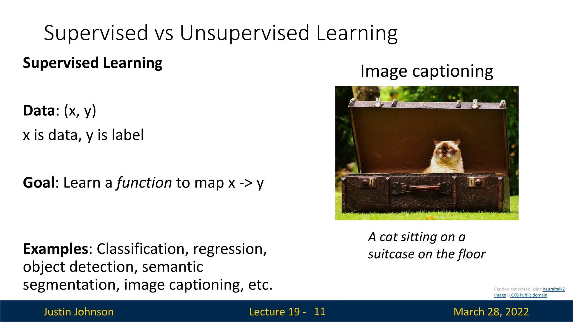
Supervised learning refers to the setting in which we are given labeled data pairs \((x, y)\), where \(x\) is the input (e.g., an image), and \(y\) is the target label (e.g., “cat”). These labels are typically human-annotated and expensive to collect at scale. This annotation burden can limit the scope of applications in data-rich but label-scarce domains.

Goal: Learn a function that maps inputs to outputs, \(f : x \rightarrow y\).

Examples: Classification, regression, object detection, semantic segmentation, image captioning.

19.1.2 Unsupervised Learning

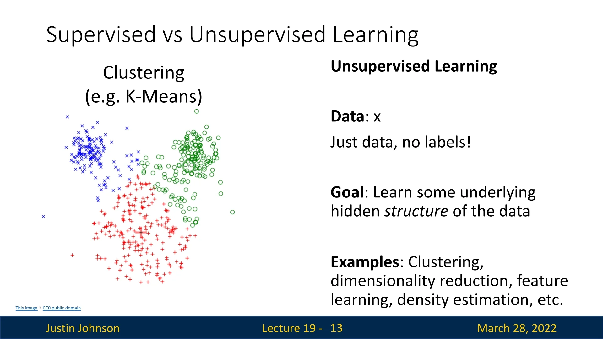
In unsupervised learning, the data comes without labels—just inputs \(x\). The goal is to extract useful structures, representations, or generative processes from the data distribution itself.

Goal: Learn a latent or hidden structure underlying the observed data.

Examples: Clustering (e.g., K-Means), dimensionality reduction (e.g., PCA), density estimation, self-supervised representation learning.

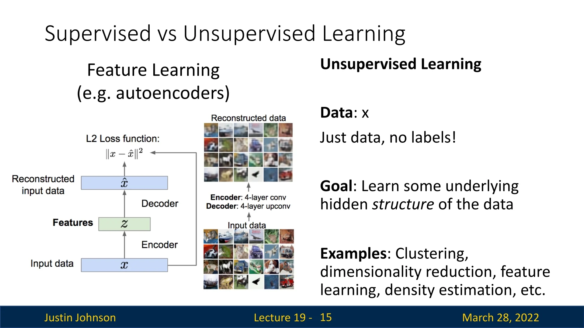
A key building block in unsupervised learning is the autoencoder, a neural network that learns to compress and reconstruct its input. By training to minimize reconstruction error, it discovers meaningful latent representations that can be used in downstream tasks [220].

Our ultimate goal is to develop methods that can learn rich and structured representations using vast amounts of unlabeled data—considered the “holy grail” of machine learning.

19.2 Discriminative vs. Generative Models

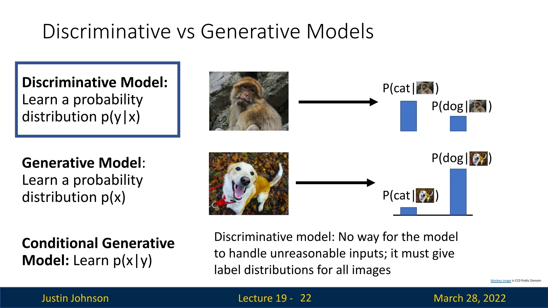
To understand the progression toward generative models, we revisit the fundamental difference between discriminative and generative modeling. Given a data point \(x\) (e.g., an image of a cat) and a label \(y\) (e.g., “cat”), we distinguish:

• Discriminative model: Learns the conditional distribution \(p(y \mid x)\).
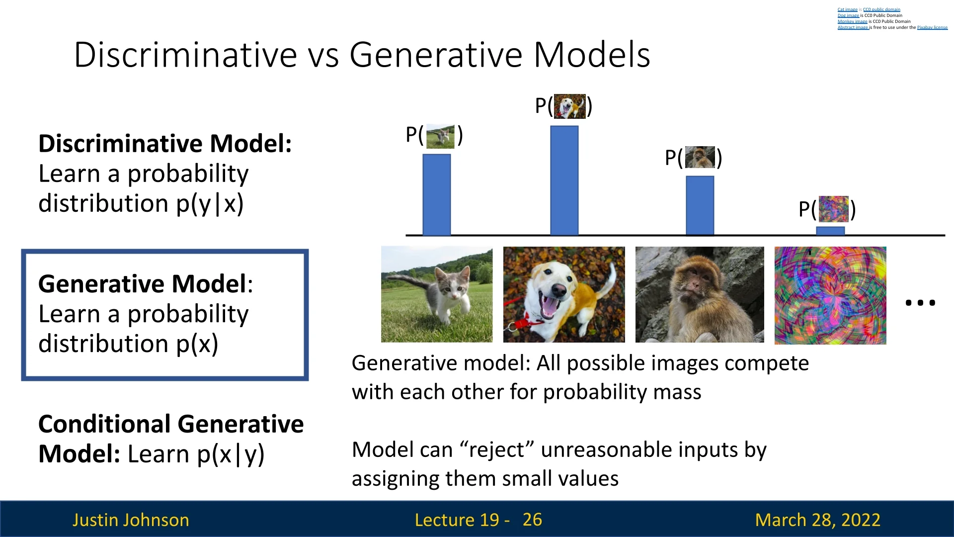
• Generative model: Learns the marginal distribution \(p(x)\).
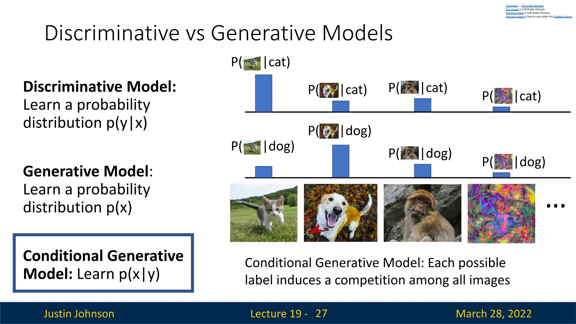
• Conditional generative model: Learns the conditional distribution \(p(x \mid y)\).

19.2.1 Discriminative Models

Discriminative models focus on classification: for a given input \(x\), what is the probability of each possible label \(y\)? The probability mass is shared among labels only—images do not compete with each other. Thus, these models are prone to confidently labeling out-of-distribution inputs.

19.2.2 Generative Models

In contrast to discriminative models, which isolate a decision boundary between classes, generative models aim to learn the full probability density \(p(x)\). This function assigns a likelihood score to every possible input configuration in the data space. This task is significantly more challenging than classification: rather than distinguishing between a finite set of labels, the model must reason over the infinite, continuous space of all possible images.

A successfully trained generative model serves two primary functions:

1.

Generation: It can synthesize new, novel samples by sampling from the learned distribution \(p(x)\).

2.

Rejection: It can detect invalid or noisy inputs by assigning them low probability density.

Because image data lies in a continuous space, the probability at any specific point is infinitesimal. Therefore, probability is only meaningful when integrated over a region. We typically evaluate likelihood-based generative models using the negative log-likelihood (NLL). For images, NLL is often reported in bits-per-dimension (bpd). A lower bpd indicates that the model assigns high density to the test data. However, high likelihood does not strictly guarantee that a sample is perceptually realistic. Generative models can sometimes assign high density to simple background textures or OOD (Out-of-Distribution) data; thus, likelihood-based anomaly detection should be used with caution.

19.2.3 Conditional Generative Models

While unconditional models learn the general concept of an image \(p(x)\), conditional generative models learn the conditional distribution \(p(x \mid y)\). Given a specific label \(y\), these models determine the likelihood of an input \(x\) belonging to that class. This offers distinct advantages over discriminative classifiers:

• Directed Synthesis: We can generate samples for a specific requested class.
• Robust Rejection: Unlike a classifier that must select the “best” label even for invalid input, a conditional generative model can reject an anomaly by assigning low likelihoods across all known labels.

19.2.4 Model Relationships via Bayes’ Rule

Our taxonomy distinguishes three complementary modeling goals:

• Discriminative: Learns \(p(y \mid x)\) (Class probability given image).
• Unconditional Generative: Learns \(p(x)\) (Image probability).
• Conditional Generative: Learns \(p(x \mid y)\) (Image probability given class).

These three families are not isolated; they are mathematically unified via Bayes’ rule:

\begin {equation} \underbrace {p(x \mid y)}_{\mbox{Conditional Gen.}} = \frac {\overbrace {p(y \mid x)}^{\mbox{Discriminative}} \cdot \overbrace {p(x)}^{\mbox{Generative}}}{p(y)}, \label {eq:chapter19_bayes_connection} \end {equation}

where \(p(y)\) represents the label prior—the frequency of each class in the dataset.

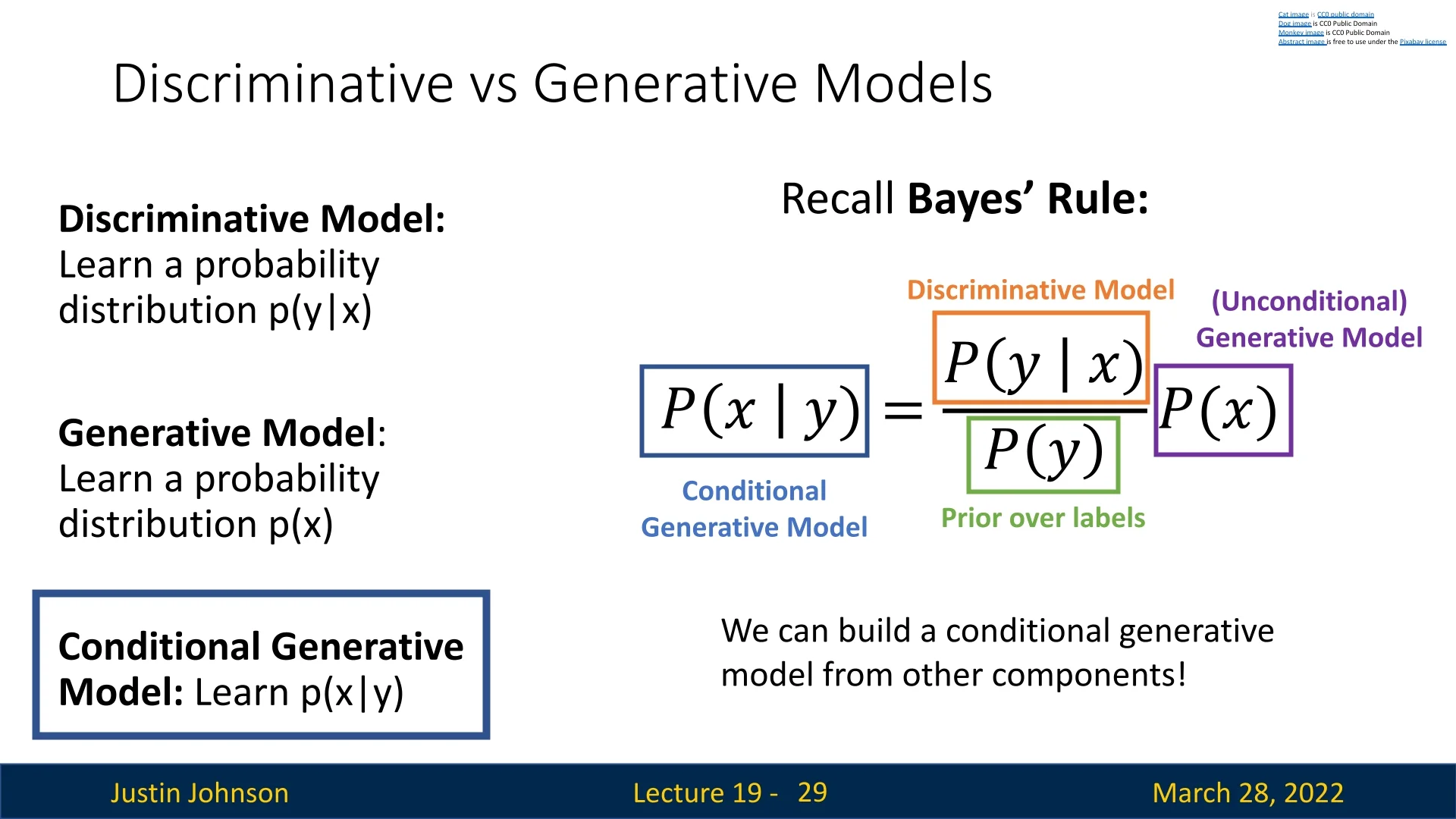
Equation 19.1 is not merely a theoretical identity; it offers concrete strategies for model construction and explains the trade-offs between different learning paradigms.

Practical Implication: Compositional Generation

The identity implies that we do not necessarily need to train a conditional generator \(p(x \mid y)\) from scratch. Instead, we can compose a conditional model from two independent components:

1.

An unconditional generator that understands realistic image statistics (\(p(x)\)).

2.

A discriminative classifier that understands semantic labels (\(p(y \mid x)\)).

This modularity is explicitly utilized in techniques such as Classifier Guidance in diffusion models, where gradients from a pre-trained classifier, \(\nabla _x \log p(y \mid x)\), are used to steer the sampling trajectory of an unconditional diffusion model toward a specific class. This allows researchers to repurpose powerful unconditional models for class-conditional tasks without expensive retraining.

Implication for Data Efficiency

The Bayesian decomposition also highlights opportunities for semi-supervised learning. Since \(p(x)\) does not require labels, the generative component can be trained on vast amounts of unlabeled data. The discriminative component \(p(y \mid x)\) can then be trained on a smaller, labeled subset. By combining them via Equation 19.1, we can construct a high-quality conditional generator \(p(x \mid y)\) even when labeled data is scarce, effectively “bootstrapping” the generation quality using the unsupervised structure learned by \(p(x)\).

In supervised settings where we model components jointly, the prior is typically approximated by empirical class frequencies: \begin {equation} \hat {p}(y) = \frac {1}{N}\sum _{i=1}^N \mathbb {I}[y_i = y]. \label {eq:chapter19_empirical_prior} \end {equation}

19.2.5 Taxonomy of Generative Models

Having established the importance of the marginal density \(p(x)\) via Bayes’ rule, we now turn to the practical challenge: how do we actually represent and learn this distribution? The space of high-dimensional images is vast, and defining a valid probability distribution over it is non-trivial.

Generative models are typically categorized based on how they approach the likelihood function \(p(x)\). The taxonomy, visualized in the below figure, distinguishes between models that explicitly define the density and those that implicitly learn to sample from it.

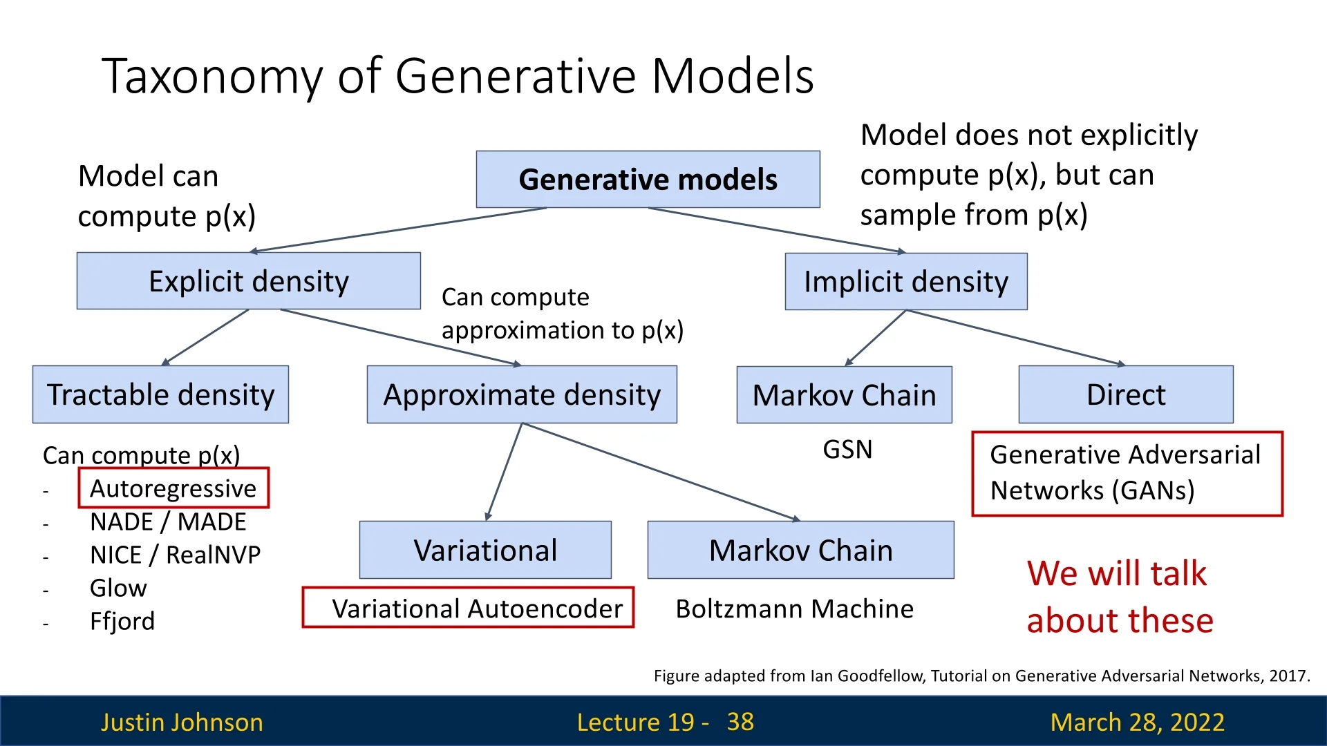
Explicit Density Models

These models construct a specific parametric function \(p_\theta (x)\) to approximate the true data distribution. They are trained by maximizing the likelihood of the training data. This family bifurcates based on mathematical tractability:

• Tractable Density: The model architecture is designed such that \(p_\theta (x)\) can be computed exactly and efficiently. This often involves imposing constraints on the model structure, such as the causal ordering in Autoregressive Models (e.g., PixelCNN) or invertible transformations in Normalizing Flows.
• Approximate Density: The model defines a density \(p_\theta (x)\) that typically involves latent variables \(z\), making the marginal likelihood \(\int p_\theta (x \mid z)p(z)dz\) intractable to compute directly. Instead, these methods optimize a proxy objective, such as the Variational Lower Bound (ELBO). Variational Autoencoders (VAEs) and Energy-Based Models (EBMs) reside here.

Implicit Density Models

In contrast, implicit models do not define an explicit likelihood function \(p_\theta (x)\) that can be evaluated. Instead, they learn a stochastic process that maps noise (e.g., \(z \sim \mathcal {N}(0, I)\)) to data space. The primary goal is to produce a sampler that generates valid data points. Generative Adversarial Networks (GANs) are the most prominent example, employing a discriminator to distinguish between real and generated samples during training.

Enrichment 19.2.6: Modern Frontiers: Diffusion and Flow Matching

The taxonomy in Figure 19.7 highlights the historical division between explicit and implicit models. However, recent state-of-the-art approaches occupy a nuanced middle ground, often described as iterative generative models or flow-based models.

Diffusion Models Diffusion Probabilistic Models (e.g., DDPM [223]) are best understood as Approximate Explicit Density models relying on Markov Chains. They define a forward process that gradually adds noise to data and learn a reverse process to denoise it. While they share the “learning to sample” spirit of implicit models (like GANs), they are mathematically grounded in optimizing a variational lower bound (ELBO) on the likelihood, placing them technically within the explicit density family.

Flow Matching Closely related are Flow Matching models [364], which unify concepts from diffusion and Continuous Normalizing Flows (CNFs). While diffusion models typically rely on stochastic differential equations (SDEs), flow matching models aim to learn a deterministic Ordinary Differential Equation (ODE) that continuously transforms a simple prior (noise) into the complex data distribution.

Unlike traditional CNFs which require expensive ODE simulation during training, flow matching employs a simulation-free objective: the model simply regresses a vector field that points along a desired probability path (often a “straight line” interpolation between noise and data). This allows for efficient training of continuous-time generative models that can compute exact likelihoods via the change of variables formula, serving as a powerful, deterministic counterpart to the stochastic diffusion framework.

Roadmap: Starting with Tractable Likelihood

Navigating this taxonomy requires building up mathematical complexity. We will begin our exploration with Autoregressive Models, which fall under the tractable explicit density category.

Autoregressive models are a natural starting point because they allow us to use the standard Principle of Maximum Likelihood without approximation. By factorizing the joint distribution of pixels into a sequence of conditional probabilities, they provide a concrete, exact mechanism for both evaluating \(p(x)\) and generating samples, serving as a foundation before we tackle the complex approximations required for VAEs and GANs.

19.3 Autoregressive Models and Explicit Density Estimation

In this section, we explore a class of generative models that aim to model the data distribution \( p_{data}(x) \) explicitly. A model is said to perform explicit density estimation when it defines a tractable density function \( p_\theta (x) \), parameterized by learnable parameters \( \theta \), which assigns a scalar likelihood to every data point \( x \).

19.3.1 Maximum Likelihood Estimation

Given a dataset \( \mathcal {D} = \{x^{(1)}, x^{(2)}, \ldots , x^{(N)}\} \) of samples drawn from the true data distribution \( p_{data} \), our goal is to find the parameters \( \theta \) such that the model distribution \( p_\theta (x) \) best approximates \( p_{data}(x) \).

To measure the closeness of these two distributions, we minimize the Kullback-Leibler (KL) divergence between the data distribution and the model: \begin {equation} D_{KL}(p_{data} \| p_\theta ) = \mathbb {E}_{x \sim p_{data}} \left [ \log p_{data}(x) - \log p_\theta (x) \right ]. \label {eq:chapter19_kl_divergence} \end {equation} Since \( \log p_{data}(x) \) is independent of \( \theta \), minimizing the KL divergence is equivalent to maximizing the expected log-likelihood of the data under the model.

The MLE Objective In practice, we do not have access to the true data distribution \( p_{data} \). Instead, we seek the parameters \( \theta \) that maximize the probability of the observed training samples under our model. This yields the principle of Maximum Likelihood Estimation (MLE): \begin {equation} \theta ^* = \arg \max _{\theta } \prod _{i=1}^N p_\theta (x^{(i)}). \label {eq:chapter19_mle_product} \end {equation} However, optimizing this product directly is rarely done in deep learning. Instead, we maximize the log-likelihood: \begin {equation} \theta ^* = \arg \max _{\theta } \sum _{i=1}^N \log p_\theta (x^{(i)}). \label {eq:chapter19_mle_log} \end {equation} Transitioning from the product in (19.4) to the sum in (19.5) is standard practice for three key reasons:

• Mathematical Validity (Monotonicity): The logarithm is a strictly monotonically increasing function. For any two values \( a \) and \( b \), if \( a > b \), then \( \log (a) > \log (b) \). Consequently, the location of the maximum is preserved: \[ \arg \max _\theta f(\theta ) = \arg \max _\theta \log (f(\theta )). \] While the value of the objective function changes, the optimal parameters \( \theta ^* \) remain identical.
• Numerical Stability: Probabilities are typically small numbers in the range \([0, 1]\). Multiplying many such values (e.g., for thousands of pixels) results in floating-point underflow, where the computer rounds the product to zero. The logarithm converts these small products into sums of negative numbers, which are numerically stable to handle.
• Optimization Efficiency: Differentiating a product of terms requires the complex product rule, leading to gradients that are difficult to compute and unstable. By converting the product to a sum, the gradient decomposes linearly (\( \nabla _\theta \sum = \sum \nabla _\theta \)), vastly simplifying backpropagation.

For explicit density models, the primary design constraint is that the function \( p_\theta (x) \) must be tractable to compute and differentiable with respect to \( \theta \), enabling us to perform this optimization efficiently.

19.3.2 Autoregressive Factorization

The joint distribution \( p(x) \) of high-dimensional data (such as an image made up of tens of thousands of pixels) is difficult to model directly due to the curse of dimensionality. Autoregressive models solve this by leveraging the chain rule of probability to decompose the joint density into a product of one-dimensional conditional distributions.

Given an input \( x \) containing \( n \) dimensions (e.g., an image with \( n \) pixels), we fix an ordering \( \{x_1, x_2, \ldots , x_n\} \). The joint probability is then factored as: \begin {equation} p_\theta (x) = \prod _{i=1}^{n} p_\theta (x_i \mid x_1, \ldots , x_{i-1}) = \prod _{i=1}^{n} p_\theta (x_i \mid x_{<i}), \label {eq:chapter19_chain_rule} \end {equation} where \( x_{<i} \) denotes all variables preceding \( x_i \) in the chosen ordering.

Raster Scan Ordering For images, a natural choice for ordering is the raster scan order (left-to-right, top-to-bottom), analogous to reading a page of text. Under this ordering, the probability of a pixel \( x_i \) is conditioned on all previously generated pixels (top-left context). This factorization transforms the problem of generative modeling into a sequence prediction task. This structure mirrors the mechanics of Recurrent Neural Networks (RNNs) in language modeling, where the network predicts the next token given the history. In the vision domain, we replace ”tokens” with ”pixel values” (typically quantized to 256 levels as in RGB images with pixel intensities ranging between 0 and 255), allowing us to apply sequence modeling architectures to image generation.

19.3.3 Recurrent Pixel Networks: Overview and Motivation

The PixelRNN framework [458] introduces a family of autoregressive models that explicitly model the joint distribution of pixels. While they differ in their internal mechanisms, they all share a unified goal: to decompose the intractable joint distribution of an image into a product of tractable conditional distributions, processed in a specific order (raster scan: row-by-row, left-to-right).

Formally, for an image \( x \) of dimensions \( H \times W \), the joint probability is factorized as: \begin {equation} p(x) = \prod _{i=1}^{H} \prod _{j=1}^{W} p(x_{i,j} \mid x_{<i, <j}), \label {eq:chapter19_pixel_factorization} \end {equation} where \( x_{<i, <j} \) denotes the context of all previously generated pixels [458].

Modeling Dependencies Between Color Channels To handle the three color channels (Red, Green, Blue), we must ensure that the generated colors within a single pixel are consistent with each other (e.g., to produce the correct hue for a specific texture). Independent prediction of channels (i.e., \(p(R)p(G)p(B)\)) would result in incoherent noise.

Therefore, we apply the chain rule of probability to split the prediction of a single pixel \( x_{i,j} \) into three sequential steps: \begin {equation} p(x_{i,j} \mid x_{<i,<j}) = p(x_{i,j}^{(R)} \mid x_{<i,<j}) \cdot p(x_{i,j}^{(G)} \mid x_{i,j}^{(R)}, x_{<i,<j}) \cdot p(x_{i,j}^{(B)} \mid x_{i,j}^{(R)}, x_{i,j}^{(G)}, x_{<i,<j}). \end {equation} This factorization is exact and ensures that the Green channel is conditioned on the Red, and the Blue is conditioned on both Red and Green [458]. While the specific order \(R \rightarrow G \rightarrow B\) is a convention (the chain rule holds for any permutation), the critical requirement is that the model captures these local inter-channel correlations.

General Architecture Pipeline

All variants in the PixelRNN family follow the same high-level processing pipeline. The architecture transforms an input image into a probability map through three stages:

1.

Input Convolution: The process begins with a \( 7 \times 7 \) masked convolution (Mask A) applied to the input image. This layer extracts low-level features while strictly enforcing causality—preventing the model from “seeing” the current pixel it is trying to predict.

2.

Core Dependency Module: This is the interchangeable component that defines the specific architecture (e.g., PixelCNN, Row LSTM). Its role is to propagate information from the spatial context \( x_{<i, <j} \) to the current position. The choice of module determines the model’s receptive field and computational efficiency.

3.

Output & Softmax: The features from the core module are projected via \( 1 \times 1 \) convolutions (Mask B) into three separate heads (one per color channel). Each head outputs a vector of 256 logits, which are passed through a Softmax function.

Why Discrete Classification? A defining feature of PixelRNN is its modeling of pixel intensities as discrete categories \( \{0, \dots , 255\} \) rather than continuous values.

Standard generative models (like VAEs) often model the conditional distribution of each pixel as a Gaussian \(\mathcal {N}(\mu , \sigma ^2)\). While VAEs typically predict a mean and variance for every pixel, the resulting distribution for any single pixel is unimodal (a single bell curve).

This restricts the model’s ability to represent ambiguous features, such as an edge that could sharply be either black (0) or white (255). A Gaussian forced to cover both possibilities must place its single peak in the middle (grey), or increase variance indiscriminately, often resulting in blurry predictions.

By treating pixel generation as a 256-way classification problem, PixelRNN can model an arbitrary multimodal distribution for each pixel. It can assign high probability to 0 and 255 simultaneously while assigning zero probability to the intermediate grey values, allowing it to generate sharp, high-frequency details without the averaging artifacts associated with unimodal continuous distributions [458].

The Architectural Landscape: Trade-offs in Context Aggregation

The PixelRNN framework proposes four specific instantiations of the Core Dependency Module, creating a spectrum of trade-offs between computational efficiency and receptive field size.

The fundamental challenge in autoregressive modeling is capturing the long-range dependencies required to generate coherent global structures (like faces or geometric shapes) while maintaining tractable training times. The paper explores this through three distinct approaches to context aggregation:

1.

Convolutional Context (PixelCNN): Uses bounded, fixed-size receptive fields via masked convolutions. This allows for massive parallelization (fast training) but restricts the model’s ability to see the “whole picture”, leading to potential blind spots.

2.

Recurrent Context (PixelRNN): Uses LSTM layers to propagate information indefinitely across the image. This theoretically captures the entire available context (infinite receptive field) but forces sequential computation, significantly slowing down training. This family splits into the Row LSTM (optimized for row-wise parallelism) and the Diagonal BiLSTM (optimized for global context).

3.

Multi-Resolution Context (Multi-Scale): An orthogonal strategy that decomposes generation into coarse and fine stages to better capture global coherence.

Enrichment 19.3.4: Legacy and Impact

While the recurrent variants (Row/Diagonal LSTM) are largely obsolete in modern practice due to their high training costs, the concepts introduced here are foundational. The analysis of blind spots in PixelCNN, the use of masked computation, and the discrete modeling of pixel values directly paved the way for the shift toward Transformer-based autoregressive models, including influential architectures like VQ-GAN [148] and ImageGPT [84].

In the following sections, we will dissect each architecture in detail, starting with the convolutional baseline before addressing its limitations with recurrent solutions.

PixelCNN

We begin our detailed study with the PixelCNN [458, 461]. While introduced alongside PixelRNN, it adopts a fully convolutional architecture. This design choice represents a significant trade-off: PixelCNN sacrifices some modeling power (due to a finite receptive field) in exchange for fast, parallel training. Unlike RNNs, which must process pixels sequentially even during training, a CNN can process the entire image at once—provided we enforce strict causality constraints.

Image Generation as Sequential Prediction Given an RGB image of size \(H \times W \times 3\), PixelCNN models the joint probability \(p(x)\) as a product of conditional probabilities over the pixels in raster-scan order (top-left to bottom-right). As defined in Eq. 19.7, this involves decomposing the joint distribution into channel-wise conditionals \(p(x_{i,j}^{(C)} \mid \dots )\).

Masked Convolutions: Enforcing Causality During training, we have access to the full ground-truth image and want to predict all conditional distributions in parallel. Standard convolutions would violate the autoregressive factorization by allowing each location to “peek” at future pixels. PixelCNN therefore uses masked convolutions that zero out any filter weights corresponding to spatial positions that are not allowed by the ordering.

The masking logic depends on the layer’s depth:

1.

Mask A (The Input Layer): The first layer involves a \(7 \times 7\) convolution applied directly to the input image [458]. Because the value at the center location \((i,j)\) in the input is the ground truth pixel we are trying to predict, strict causality requires that the filter blocks the center position. It can only access pixels strictly above or to the left.

2.

Mask B (The Residual Body): Subsequent layers (typically \(3 \times 3\)) process feature maps, not raw pixels. The feature vector at location \((i,j)\) in layer \(L\) contains aggregated information from the context of \((i,j)\) found in layer \(L-1\). To propagate this context information forward, the filter must allow access to the center position. Mask B therefore unblocks the center weight (allowing “self-connection” of features) while continuing to block all future spatial positions [458].

Channel-Aware Masking In addition to spatial masking, PixelCNN must respect the chain rule for color channels: \(p(R) \cdot p(G|R) \cdot p(B|R,G)\). PixelCNN implements this by splitting the output feature maps at every layer into three groups corresponding to R, G, and B. The masks are adjusted to enforce inter-group connectivity constraints [458]:

• Group R: Can only access context from spatial predecessors.
• Group G: Can access spatial predecessors and the current spatial position’s R features.
• Group B: Can access spatial predecessors and the current spatial position’s R and G features.

class MaskedConv2d(nn.Conv2d):


"""
Implements a convolution with a spatial mask to enforce autoregressive ordering.

Args:
mask_type (str): ’A’ for the first layer (blocks center pixel),
’B’ for subsequent layers (allows center pixel).
"""


def __init__(self, in_channels, out_channels, kernel_size, mask_type=’A’):
    super().__init__(
        in_channels, out_channels,
        kernel_size, padding=kernel_size // 2, bias=True
    )
    assert mask_type in {’A’, ’B’}
    self.mask_type = mask_type

    # Register a buffer for the mask (saved with model, but not trained)
    self.register_buffer(’mask’, torch.ones_like(self.weight))

    kH, kW = self.kernel_size
    yc, xc = kH // 2, kW // 2

    # 1. Spatial Masking: Block all future positions
    # Zero out all rows below the center
    self.mask[:, :, yc+1:, :] = 0
    # Zero out all columns to the right of the center in the center row
    self.mask[:, :, yc, xc+1:] = 0

    # 2. Center Pixel Logic (Spatial component only)
    if mask_type == ’A’:
        # In the first layer, we must not see the input pixel at all.
        self.mask[:, :, yc, xc] = 0
    else:  # mask_type == ’B’
        # In hidden layers, we can see the feature at the center
        # (which is derived from past context).
        self.mask[:, :, yc, xc] = 1

    # NOTE: This code implements the SPATIAL mask.
    # The channel-grouping mask (e.g., R->G) is typically applied
    # by manually zeroing out specific blocks of self.mask[:, :, yc, xc]
    # after initialization, or by splitting the feature maps.


def forward(self, x):
    # Apply the mask to the weights before convolution
    weight = self.weight * self.mask
    return F.conv2d(
        x, weight, self.bias,
        self.stride, self.padding, self.dilation, self.groups
    )

Trace: Processing a Sample \(4 \times 4\) Image To demystify the interaction between spatial locations and color channels, let us trace exactly how the network processes information for a specific pixel location \((2,2)\) in an image of size \(4 \times 4\) with 3 color channels.

Setup: Feature Groups and Tensor Shapes Consider a standard PixelCNN with a hidden dimension of \(h = 120\) channels. These 120 channels are not generic; they are logically divided into three groups of 40 channels each:

• Group \(h_R\) (Channels 0-39): Features dedicated to modeling the Red context.
• Group \(h_G\) (Channels 40-79): Features dedicated to modeling the Green context.
• Group \(h_B\) (Channels 80-119): Features dedicated to modeling the Blue context.

Every convolution kernel in the network has the shape \([C_{out}, C_{in}, k_H, k_W]\). The mask is a binary tensor of the same shape applied to these weights.

Step 1: The Input Layer (Mask A) The first layer transforms the raw input image \((B, 3, 4, 4)\) into the first hidden state \((B, 120, 4, 4)\).

• Input: The raw pixel at \((2,2)\) consists of 3 values: \(R, G, B\).

• Spatial Masking (The \(k_H \times k_W\) grid): Before considering color, we must enforce spatial causality. For every filter in the bank:

  • Future Rows: Weights for all rows below the center (e.g., row 3 in a \(3 \times 3\) kernel) are set to 0.
  • Future Columns: In the center row, weights for all columns to the right of the center are set to 0.
  • Past Context: Weights for rows above the center and columns to the left are set to 1 (allowed).

• Center Pixel Masking (The \(120 \times 3\) matrix): At the exact center spatial position \((1,1)\), we are left with the connections between input colors and output features. Mask A enforces the specific dependencies \(R \to G \to B\): \[ \mbox{Mask}_A = \bordermatrix { & \mbox{Input } R & \mbox{Input } G & \mbox{Input } B \cr \mbox{Out } h_R & 0 & 0 & 0 \cr \mbox{Out } h_G & 1 & 0 & 0 \cr \mbox{Out } h_B & 1 & 1 & 0 } \]

  • Row 1 (\(h_R\)): All zeros. The Red filters cannot see any current pixel value. They rely solely on the spatial context gathered from neighbors.
  • Row 2 (\(h_G\)): The column for Input R is 1. The Green filters can see the current Red value.
  • Row 3 (\(h_B\)): Columns for Input R and G are 1. The Blue filters can see current Red and Green values.
• Result: The \(h_R\) features at \((2,2)\) are derived only from spatial neighbors. The \(h_G\) features contain the exact ground truth Red value.

Step 2: The Hidden Layers (Mask B) Subsequent layers map the 120-channel hidden state to a new 120-channel hidden state.

• Spatial Masking: Identical to Step 1. We must always block future spatial positions (rows below, columns right) to prevent leakage from future pixels like \((3,0)\).

• Center Pixel Masking (The \(120 \times 120\) matrix): At the center spatial position, we must prevent information leakage between groups. \[ \mbox{Mask}_B = \bordermatrix { & \mbox{In } h_R & \mbox{In } h_G & \mbox{In } h_B \cr \mbox{Out } h_R & 1 & 0 & 0 \cr \mbox{Out } h_G & 1 & 1 & 0 \cr \mbox{Out } h_B & 1 & 1 & 1 } \]

  • Row 1 (\(h_R\)): Can read from Input \(h_R\) (1). This is safe because Input \(h_R\) from the previous layer was already blind to the current pixel. This “pass-through” allows the network to process spatial context deeply.
  • Row 1 Leaks: The Red output block must have 0s for columns corresponding to \(h_G\) and \(h_B\). If it read from \(h_G\), it would indirectly access the Red pixel value (which \(h_G\) sees), violating the masked prediction task.

Step 3: Prediction and Inference vs. Training The final layer projects the features to 256 logits for each color. The behavior here differs fundamentally between training and inference. A. During Training (Teacher Forcing) We have the full ground truth image \(X\). We feed \(X\) into the network.

• Due to Mask A/B, the Red logits at \((2,2)\) are computed without seeing \(R_{2,2}\).
• The Green logits at \((2,2)\) are computed seeing \(R_{2,2}\) (the true value) via the \(h_G\) stream.
• The Blue logits at \((2,2)\) are computed seeing \(R_{2,2}\) and \(G_{2,2}\) via the \(h_B\) stream.
• Parallelism: We can compute the loss for all 3 channels and all pixels in a single forward pass because the masks ensure that no prediction “sees itself” or its future.

B. During Inference (Autoregressive Sampling) We do not have the ground truth. We must generate it step-by-step.

1.

Predict Red: We run the network. The \(h_R\) stream predicts Red based on spatial neighbors. We sample \(r_{sim}\).

2.

Inject Red: We write \(r_{sim}\) into the input image tensor at position \((2,2)\).

3.

Predict Green: We run the network again. Now, the \(h_G\) stream (via Mask A) reads the value \(r_{sim}\) we just wrote. It predicts Green conditioned on this sampled value. We sample \(g_{sim}\).

4.

Predict Blue: We write \(g_{sim}\) into the image. The \(h_B\) stream reads both \(r_{sim}\) and \(g_{sim}\). We sample \(b_{sim}\).

This sequential injection of sampled values is why inference requires \(3 \times H \times W\) passes, whereas training requires only one.

Why is the First Pixel Random? At pixel \((0,0)\), the spatial masks block all neighbors (padding is zero).

• Training: Mask A blocks the center inputs. The network sees strictly zeros. It optimizes its weights so that \(f(\mathbf {0}) \approx P(\mbox{dataset color distribution})\).
• Inference: The network sees zeros and outputs that fixed prior distribution. The randomness comes solely from the sampling operation (e.g., torch.multinomial). If we sample a rare color, the context for \((0,1)\) changes, sending the generation down a unique path.

Inference: The Sequential Bottleneck The dependency structure imposes a strict hierarchy that dictates the generation order. We cannot generate the Red channel for all pixels first, because the Red value at position \((0,1)\) depends on the Blue value at position \((0,0)\).

Therefore, inference must proceed pixel-by-pixel in raster order, and channel-by-channel within each pixel. The complete generation sequence is:

1.

Pixel 1: Predict Red \(\to \) Sample \(\to \) Predict Green \(\to \) Sample \(\to \) Predict Blue \(\to \) Sample.

2.

Pixel 2: Predict Red (conditioned on Pixel 1) …

Consequently, generating an entire image requires \(3 \times H \times W\) sequential forward passes. Unlike training, which is fully parallelizable (\(O(1)\)), sampling scales linearly with the number of sub-pixels (\(O(N)\)), making PixelCNNs extremely slow for high-resolution synthesis.

Why Move Beyond PixelCNN? Blind Spots and Receptive Fields Despite its training efficiency, the standard PixelCNN architecture suffers from geometric flaws that limit its modeling performance:

• Limited Receptive Field: The receptive field of a CNN grows linearly with depth. To capture long-range dependencies (e.g., correlating the top of a face with the chin), the network requires a prohibitive number of layers.
• The Blind Spot Problem: As analyzed in the Gated PixelCNN work [461], simple masked convolutions suffer from a geometric “blind spot.” Due to the rectangular nature of the mask, the kernel cannot access pixels located to the right of the center in previous rows. Although these pixels are in the past (and thus valid context), the masked kernel simply cannot reach them. As layers stack, this creates a triangular region of valid context that is permanently invisible to the model, ignoring potentially crucial information.

These limitations—specifically the inability to access the full global context—motivate the use of recurrent architectures, which we explore next: the Row LSTM and Diagonal BiLSTM.

Row LSTM

The Row LSTM represents a paradigm shift from the purely feed-forward stacks of PixelCNN to a recurrent architecture. While PixelCNN attempts to build a large receptive field by stacking many fixed-size convolution layers, Row LSTM aggregates context explicitly by maintaining a state vector that propagates down the image, row by row. This design allows for the capture of vertical long-range dependencies with theoretically infinite reach, although it introduces its own geometric limitations.

Architecture Overview: From Convolution to Recurrence The single-scale Row LSTM network follows a structured pipeline designed to balance recurrent modeling with parallel efficiency [458]:

1.

Initial Feature Extraction (Mask A). The raw RGB image \(x \in \mathbb {R}^{3 \times H \times W}\) is first passed through a \(7 \times 7\) masked convolution (Mask A), producing a feature map \[ \mathbf {X} \in \mathbb {R}^{h \times H \times W}, \quad h \gg 3. \] This layer serves two purposes:

• It embeds raw pixels into a higher-dimensional feature space suitable for the LSTM (typically \(h=128\) or more).
• Its mask enforces both spatial causality (no access to pixels below or to the right) and the within-pixel \(R \to G \to B\) ordering, exactly as in PixelCNN’s first layer.

From this point onward, the Row LSTM operates on \(\mathbf {X}\) and its transformed versions; it never sees raw RGB values directly.

2.

Row-wise Recurrent Stack. The feature map \(\mathbf {X}\) is then fed into a stack of Row LSTM layers. Each Row LSTM layer treats the image as a sequence of rows, processed in order \(i = 1, \dots , H\). The row index \(i\) acts as the “time” step of the RNN.

To clarify the distinction between the “row state” (the recurrent unit) and the “pixel state” (the per-location slice), it is helpful to make the geometry of the Row LSTM completely explicit:

• Row-level state maps (the computational unit): At recurrent step \(i\) (corresponding to image row \(i\)), the Row LSTM maintains a hidden map \(\mathbf {h}_i \in \mathbb {R}^{h \times W}\) and a cell map \(\mathbf {c}_i \in \mathbb {R}^{h \times W}\). Once the previous row state \((\mathbf {h}_{i-1}, \mathbf {c}_{i-1})\) is known, the update for row \(i\) is computed in a single parallel step across all columns. There is no left-to-right recurrence within the row; horizontal coupling happens only through the convolution kernels [458].
• Pixel-level slices (the conceptual unit): The vector \(\mathbf {h}_{i,j} \in \mathbb {R}^{h}\) is simply the column-\(j\) slice of the row map \(\mathbf {h}_i\). When we say that \(\mathbf {h}_{i,j}\) depends on “neighbors” in the previous row, we mean the specific columns of \(\mathbf {h}_{i-1}\) that fall under the 1D convolution kernel. For a kernel width \(k\), the recurrent convolution \(\mathbf {K}^{ss}\) accesses the neighborhood \(\mathbf {h}_{i-1,\, j-(k-1)/2} \dots \mathbf {h}_{i-1,\, j+(k-1)/2}\) (with appropriate padding).

• Channel grouping (implementing \(R \to G \to B\)): As in PixelCNN, the \(h\) hidden channels at each spatial location are conceptually partitioned into three groups \[ \mathbf {h}_{i,j} = \big [ \mathbf {h}_{i,j}^{(R)}, \; \mathbf {h}_{i,j}^{(G)}, \; \mathbf {h}_{i,j}^{(B)} \big ]. \]

  A single Row LSTM layer thus learns all three color-conditionals jointly. The \(R \to G \to B\) dependency is enforced by masks applied to the input-to-state convolution: the connections into the gates that control \(\mathbf {h}^{(R)}\) are masked to be blind to the current pixel’s raw intensities, those into \(\mathbf {h}^{(G)}\) are allowed to see the current Red value, and those into \(\mathbf {h}^{(B)}\) are allowed to see both Red and Green. This mirrors the Mask A / Mask B logic from PixelCNN, but embedded inside the Row LSTM’s convolutional gates [458].

The Convolutional LSTM Mechanism To preserve spatial structure, the Row LSTM replaces the fully connected mappings of a standard LSTM with 1D convolutions aligned with the row direction. Following [458], the update for row \(i\) decomposes into two linear terms—an input-to-state term and a state-to-state term—followed by pointwise gate nonlinearities.

The gate pre-activations are defined as: \begin {align} [\mathbf {o}_i, \mathbf {f}_i, \mathbf {i}_i, \mathbf {g}_i] &= \underbrace {\mathbf {K}^{ss} \circledast \mathbf {h}_{i-1}}_{\mathbf {V}_i \;\text {(recurrent term)}} + \underbrace {\mathbf {K}^{is} \circledast \mathbf {x}_i}_{\mathbf {U}_i \;\text {(input term)}}, \label {eq:chapter19_rowlstm_gates} \end {align}

where:

• \(\circledast \) denotes a 1D convolution along the width of the row.
• \(\mathbf {h}_{i-1} \in \mathbb {R}^{h \times W}\) is the hidden state map of the previous row (computed in the previous step).
• \(\mathbf {x}_i \in \mathbb {R}^{h \times W}\) is the feature map of the current row (from the previous layer or initial embedding).
• \(\mathbf {K}^{ss}\) and \(\mathbf {K}^{is}\) are convolution kernels producing \(4h\) output channels (one block of \(h\) channels per gate).

The state updates follow standard LSTM logic (applied elementwise at every position \((i,j)\)): \begin {align} \mathbf {c}_i &= \sigma (\mathbf {f}_i) \odot \mathbf {c}_{i-1} + \sigma (\mathbf {i}_i) \odot \tanh (\mathbf {g}_i), \label {eq:chapter19_rowlstm_cell} \\ \mathbf {h}_i &= \sigma (\mathbf {o}_i) \odot \tanh (\mathbf {c}_i), \label {eq:chapter19_rowlstm_hidden} \end {align}

where \(\sigma (\cdot )\) is the logistic sigmoid and \(\tanh (\cdot )\) is the hyperbolic tangent.

Decomposition and Concurrency. The computation in Eq. (19.5) is implemented in two phases to maximize GPU efficiency [458]:

1.

Input-to-state map \(\mathbf {U}\): precomputed for all rows.

• Before the recurrent loop, we apply a single masked \(k \times 1\) convolution with kernel \(\mathbf {K}^{is}\) to the entire feature map \(\mathbf {X}\) (all rows and columns at once), obtaining \(\mathbf {U} \in \mathbb {R}^{4h \times H \times W}\).
• This convolution uses Mask B to strictly enforce the autoregressive constraints.
• During the recurrent loop, we simply index \(\mathbf {U}_i\) as the input term for row \(i\).

2.

State-to-state map \(\mathbf {V}_i\): computed row-by-row.

• For each row \(i\), after \(\mathbf {h}_{i-1}\) is known, we compute \(\mathbf {V}_i = \mathbf {K}^{ss} \circledast \mathbf {h}_{i-1}\).
• This is an unmasked 1D convolution. Because row \(i-1\) is fully in the past, no causality constraints are violated, and the convolution may freely mix all channel groups (e.g., Red features in row \(i\) can read from Green/Blue features in row \(i-1\)).
• We then sum \(\mathbf {V}_i + \mathbf {U}_i\) to get the gates and update the states.

Trace: The Triangular Receptive Field (4\(\times \)4 Example) To make the geometry concrete, let us trace the dependency pattern for pixel \((2,2)\) in a \(4 \times 4\) image (using 0-based indexing: rows/columns \(0,1,2,3\)). We assume a kernel width of \(k=3\).

Step 0: How \(\mathbf {U}\) and \(\mathbf {u}_{2,2}\) are constructed.

Before the Row LSTM loop over rows begins, we precompute the input-to-state term for all rows and columns: \begin {equation} \mathbf {U} = \mathbf {K}^{is} \circledast \mathbf {X}, \end {equation} where:

• \(\mathbf {X} \in \mathbb {R}^{c_{\mbox{in}} \times H \times W}\) is the feature map produced by the initial \(7 \times 7\) Mask A convolution (or by the previous Row LSTM layer).
• \(\mathbf {K}^{is}\) is a masked convolution kernel of size \(k \times 1\), applied along the width with Mask B to enforce spatial causality and the \(R \to G \to B\) constraints.
• The result \(\mathbf {U} \in \mathbb {R}^{4h \times H \times W}\) contains, at each location \((i,j)\), the pre-activation contributions for the four LSTM gates (output, forget, input, content) for all \(h\) channels.

During the recurrent loop, we simply index into this tensor row-by-row: \begin {align*} \mathbf {U}_i &= \mathbf {U}[:, i, :] \in \mathbb {R}^{4h \times W}, \\ \mathbf {u}_{i,j} &= \mathbf {U}[:, i, j] \in \mathbb {R}^{4h}, \end {align*}

so \(\mathbf {u}_{2,2}\) is exactly the \(4h\)-dimensional vector stored at row \(i=2\), column \(j=2\) of \(\mathbf {U}\). It encodes all contributions to the gates at \((2,2)\) coming from the current-row features \(\mathbf {x}_2\).

Because \(\mathbf {U}\) was computed via a masked \(k \times 1\) convolution along the width, the input-to-state term at \((2,2)\) depends only on a local horizontal neighborhood of the current row: \begin {equation} \mathbf {u}_{2,2} = \big (\mathbf {K}^{is} \circledast \mathbf {x}_2\big )_{:, 2} \quad \Rightarrow \quad \mathbf {u}_{2,2} \mbox{ is a function of } \{\mathbf {x}_{2,1}, \mathbf {x}_{2,2}, \mathbf {x}_{2,3}\}, \end {equation} for kernel width \(k=3\) and appropriate causal masking.

Step 1: Row-level dependency (vertical recurrence).

Inside the Row LSTM loop, each row \(i\) is updated using the decomposition \begin {align*} [\mathbf {o}_i, \mathbf {f}_i, \mathbf {i}_i, \mathbf {g}_i] &= \mathbf {V}_i + \mathbf {U}_i, \qquad \mathbf {V}_i = \mathbf {K}^{ss} \circledast \mathbf {h}_{i-1}, \end {align*}

where \(\mathbf {K}^{ss}\) is an unmasked 1D convolution kernel of width \(k\). At step \(i=2\):

• The previous-row hidden map \(\mathbf {h}_1 \in \mathbb {R}^{h \times W}\) is already known.
• We compute \(\mathbf {V}_2 = \mathbf {K}^{ss} \circledast \mathbf {h}_1\), obtaining \(\mathbf {V}_2 \in \mathbb {R}^{4h \times W}\) for all columns \(j=0,\dots ,3\) in a single parallel operation.
• The gate pre-activations for row \(2\) are then \(\mathbf {V}_2 + \mathbf {U}_2\) and are transformed into \((\mathbf {c}_2, \mathbf {h}_2)\) via the usual LSTM nonlinearities.

Step 2: Pixel-level view at \((2,2)\): vertical expansion.

Focus now on the specific hidden vector \(\mathbf {h}_{2,2}\), the column-\(2\) slice of \(\mathbf {h}_2\). It is determined by the gate pre-activations at \((2,2)\): \begin {align*} \mathbf {v}_{2,2} &= \big (\mathbf {K}^{ss} \circledast \mathbf {h}_1\big )_{:,2}, \\ \mathbf {u}_{2,2} &= \big (\mathbf {K}^{is} \circledast \mathbf {x}_2\big )_{:,2}, \\ [\mathbf {o}_{2,2}, \mathbf {f}_{2,2}, \mathbf {i}_{2,2}, \mathbf {g}_{2,2}] &= \mathbf {v}_{2,2} + \mathbf {u}_{2,2}, \\ \mathbf {c}_{2,2} &= \sigma (\mathbf {f}_{2,2}) \odot \mathbf {c}_{1,2} + \sigma (\mathbf {i}_{2,2}) \odot \tanh (\mathbf {g}_{2,2}), \\ \mathbf {h}_{2,2} &= \sigma (\mathbf {o}_{2,2}) \odot \tanh (\mathbf {c}_{2,2}). \end {align*}

Because \(\mathbf {K}^{ss}\) is a width-\(3\) convolution, the recurrent term at \((2,2)\) aggregates information from a 3-pixel neighborhood in the previous row: \begin {equation} \mathbf {v}_{2,2} \;\mbox{depends on}\; \{\mathbf {h}_{1,1}, \mathbf {h}_{1,2}, \mathbf {h}_{1,3}\}. \end {equation} Each of these previous-row states was, in turn, computed from a similar 3-pixel neighborhood in row \(0\), and so on. As we trace this dependency upwards, the horizontal span of influencing pixels expands by roughly one column on each side per row, forming an inverted triangular receptive field above \((2,2)\).

Step 3: Horizontal limitation within row \(2\).

The key limitation is horizontal coverage within the current row:

• The Row LSTM has no left-to-right recurrence inside row \(2\). There is no direct connection \(\mathbf {h}_{2,1} \to \mathbf {h}_{2,2}\); the recurrent path runs only from \(\mathbf {h}_{1,\cdot }\) to \(\mathbf {h}_{2,\cdot }\).
• Consequently, horizontal information from row \(2\) enters \(\mathbf {h}_{2,2}\) only through the input-to-state term \(\mathbf {u}_{2,2}\), which was produced by a width-\(3\) masked convolution over \(\mathbf {x}_2\).
• For \(k=3\), the receptive field of \(\mathbf {u}_{2,2}\) in row \(2\) is limited to the local window \( \{ \mathbf {x}_{2,1}, \mathbf {x}_{2,2}, \mathbf {x}_{2,3} \}. \)
• In particular, the feature \(\mathbf {x}_{2,0}\) (or equivalently, the pixel at \((2,0)\)) lies outside this kernel window. Since there is no horizontal recurrence to propagate information from \((2,0)\) through \(\mathbf {h}_{2,1}\) to \(\mathbf {h}_{2,2}\), the current Row LSTM layer has no path for \((2,0)\) to influence \((2,2)\).

Blind-spot consequence.

Combining vertical expansion (via \(\mathbf {v}_{2,2}\)) and local horizontal access (via \(\mathbf {u}_{2,2}\)), the receptive field of \(\mathbf {h}_{2,2}\) in a single Row LSTM layer is an inverted triangle that does not cover all pixels above and to the left that are valid under the raster ordering. Concretely:

• Pixels like \((2,0)\) in the same row, which are earlier in raster order, are not reachable if they fall outside the local convolution window.
• Pixels far to the left or right in earlier rows may also fall outside the triangular region reached by repeated applications of the width-\(3\) convolution.

These unreachable regions form a blind spot in the receptive field. This geometric limitation motivates the Diagonal BiLSTM, which reorganizes computation along diagonals so that, for each pixel, the receptive field can cover all previously generated pixels [458].

Handling Color Channels: Training vs. Inference Row LSTM uses the same masking logic as PixelCNN to model RGB dependencies within each pixel using a single shared network.

A. During Training (Parallel Teacher Forcing) We feed the full ground truth image \(X\).

• The masked \(\mathbf {K}^{is}\) kernel ensures that \(\mathbf {h}^{(G)}\) is computed using the ground truth Red value from the input, while \(\mathbf {h}^{(R)}\) is computed without it.
• Because we have the ground truth, we can compute the gates and updates for all channels and all pixels in a row in parallel. The sequential operation is only row-by-row.

B. During Inference (Sequential Sampling) At test time, the ground truth is unknown, so we must generate the image one pixel at a time. Since the model treats pixel intensities as discrete categories rather than continuous values, the output for each color channel is a 256-way Softmax distribution representing the probability of every possible intensity \(v \in \{0, \dots , 255\}\).

The generation for a single pixel at \((i,j)\) proceeds in a three-step micro-sequence:

1.

Sample Red: The network outputs a 256-dimensional vector of logits for the Red channel at \((i,j)\). We apply a Softmax to obtain probabilities and sample a discrete intensity \(r\) from this categorical distribution (rather than simply taking the argmax, which would be deterministic).

2.

Sample Green: We feed the chosen value \(r\) back into the network. The masked filters allow the Green group to “see” this value, producing a new 256-way Softmax distribution for Green conditioned on Red. We sample an intensity \(g\).

3.

Sample Blue: We feed \(r\) and \(g\) back into the network. The Blue group produces a distribution conditioned on both. We sample \(b\).

This forces the generation process to be sequential both spatially (raster order) and channel-wise (\(R \to G \to B\)).

Looking Ahead To overcome this asymmetry, the Diagonal BiLSTM variant (explored next) modifies the recurrence pattern to follow image diagonals. This enables more balanced 2D coverage in a single layer — expanding the receptive field in both directions more efficiently.

Diagonal BiLSTM

The Diagonal BiLSTM addresses the geometric limitations of the Row LSTM by fundamentally changing the order in which the image is traversed. Instead of processing the image row-by-row (which creates a blind spot), it generates the image diagonal-by-diagonal. A diagonal is defined as the set of pixels where \( r + c = \mbox{const} \).

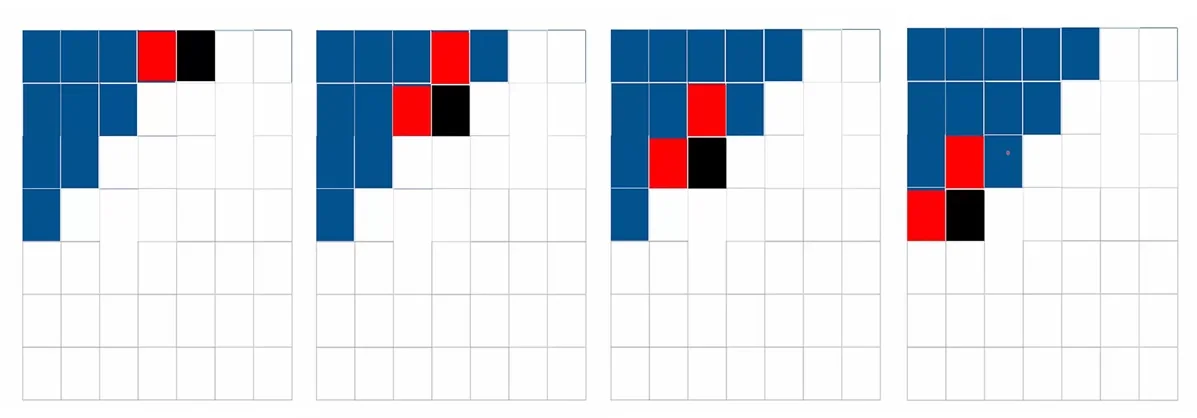
From Rows to Diagonals via Skewing Directly convolving along diagonals in a standard grid is computationally inefficient due to memory access patterns. The Diagonal BiLSTM solves this by skewing the feature map so that diagonals in the original image become vertical columns in the new map.

• The Transformation: We transform the input map \(\mathbf {X} \in \mathbb {R}^{h \times H \times W}\) into a skewed map \(\tilde {\mathbf {X}}\) by shifting each row \(i\) to the right by \(i\) positions. \[ \mbox{Original } (i, j) \quad \longrightarrow \quad \mbox{Skewed } (i, j+i) \] The resulting map has shape \(H \times (W + H - 1)\).

• Why Skewing Works: In this skewed coordinate system, the two autoregressive neighbors of pixel \((i, j)\)—its left neighbor \((i, j-1)\) and top neighbor \((i-1, j)\)—align perfectly into a vertical column:

  • Left Neighbor \((i, j-1)\): Moves to column \((j-1) + i = (i+j) - 1\). This is the previous column, same row.
  • Top Neighbor \((i-1, j)\): Moves to column \(j + (i-1) = (i+j) - 1\). This is the previous column, previous row.
• The Kernel: Because both neighbors land in the previous column of the skewed map, a simple \(2 \times 1\) convolution (height 2, width 1) applied to the previous column can capture both the Top and Left context simultaneously.

The Convolutional LSTM Mechanism Once skewed, the Diagonal BiLSTM operates like a standard LSTM where the “time” axis is the diagonal index \(d\). For each diagonal \(d\), the layer maintains hidden and cell maps \(\mathbf {h}_d, \mathbf {c}_d \in \mathbb {R}^{h \times H}\). Each column of these maps corresponds to one pixel on the diagonal after unskewing.

As in the Row LSTM, the gate pre-activations are decomposed into an input-to-state term \(\mathbf {U}_d\) (independent of recurrence) and a state-to-state term \(\mathbf {V}_d\) (recurrent along diagonals).

1.

Input-to-State Map (\(\mathbf {U}\)): Shared and Precomputed. We first compute an input tensor \(\mathbf {U}\) for all diagonals in parallel by applying a masked \(1 \times 1\) convolution to the skewed feature map \(\tilde {\mathbf {X}}\): \[ \mathbf {U} = \mathbf {K}^{is} \circledast \tilde {\mathbf {X}}. \] Since the kernel is \(1 \times 1\), this step does not mix information between diagonals or rows; it purely transforms features and applies the Mask B channel masks to enforce the \(R \to G \to B\) dependency groups. The slice \(\mathbf {U}_d\) is reused by both directional streams.

2.

State-to-State Map (\(\mathbf {V}_d\)): The \(2 \times 1\) Recurrent Convolution.

For a given direction, the recurrent contribution for diagonal \(d\) is obtained by convolving the previous diagonal’s hidden map with a vertical \(2 \times 1\) kernel: \[ \mathbf {V}_d = \mathbf {K}^{ss} \circledast \mathbf {h}_{d-1}. \] Here, we treat the skewed hidden states as a tensor \(\tilde {\mathbf {H}}\) where \(\mathbf {h}_{d-1}\) is the column corresponding to the previous time step. Applying a \(2 \times 1\) convolution to this column means:

• For each output row index \(r\) on the current diagonal \(d\), the kernel looks at a 2-pixel vertical window in the previous diagonal: the vector at row \(r\) and the vector at row \(r-1\) (with zero-padding at the top).

• Geometric Mapping: These two stacked positions correspond exactly to the spatial neighbors in the original image:

  • \(\mathbf {h}_{d-1}[r, :]\) maps to the Left neighbor \((r, c-1)\).
  • \(\mathbf {h}_{d-1}[r-1, :]\) maps to the Top neighbor \((r-1, c)\).

  Both neighbors map to column \(d-1\) in the skewed grid because \((r) + (c-1) = (r-1) + c = r+c-1 = d-1\).

Concretely, if \(\mathbf {W}^{(0)}\) and \(\mathbf {W}^{(1)}\) are the weights of the \(2 \times 1\) kernel \(\mathbf {K}^{ss}\), the pre-activation for row \(r\) is computed as: \[ \mathbf {V}_d[r, :] = \mathbf {W}^{(0)} \mathbf {h}_{d-1}[r, :] + \mathbf {W}^{(1)} \mathbf {h}_{d-1}[r-1, :]. \] This operation is unmasked because all pixels on diagonal \(d-1\) are strictly in the past relative to diagonal \(d\). Therefore, the convolution can freely mix information across all channels, allowing the Red features of the current pixel to learn from the Green and Blue features of its neighbors [458].

The gate pre-activations for diagonal \(d\) are then simply the sum \(\mathbf {U}_d + \mathbf {V}_d\), followed by the standard elementwise LSTM updates for \(\mathbf {c}_d\) and \(\mathbf {h}_d\) as in the Row LSTM case.

Bidirectionality and Causal Correction A single Diagonal LSTM stream propagates context in only one direction along the diagonals (e.g., scanning from top-left to bottom-right). While this stream covers the causal past in theory, the paths information must take are highly anisotropic. Information from the top-left flows downwards and rightwards very efficiently, whereas information from the top-right is structurally cut off or must travel through convoluted paths.

• Directional Bias (The ”Blind Spot”). Consider the current pixel \((i, j)\).

  • Top-Left Context (Easy): A pixel like \((i, j-10)\) is connected to \((i, j)\) by a direct chain of ”Right” moves (propagated via the Left-neighbor tap in the kernel). The path length is proportional to the spatial distance.
  • Top-Right Context (Hard/Zig-Zag): A pixel like \((i, j+10)\) is spatially close but topologically distant. In a forward stream that only connects to Top and Left neighbors, there is no direct link pulling information from the right. To reach \((i, j)\), a signal from \((i, j+10)\) would conceptually have to travel ”Left” (against the stream) or find a common ancestor far up in the image (e.g., at row \(0\)) and travel down. We call these hypothetical inefficient paths ”zig-zag” paths because they would require traversing deep into the past and back, which is effectively impossible in a single layer.

• The Solution (Dual Streams). Diagonal BiLSTM addresses this by running two independent LSTM streams that sweep the image in opposite directions:

  • Forward Stream (\(\mathbf {h}^{\mathrm {fwd}}\)): Scans diagonals \(0 \to D\). Its kernel connects to \((r, c-1)\) and \((r-1, c)\), efficiently capturing the Top-Left half-plane.

  • Reverse Stream (\(\mathbf {h}^{\mathrm {rev}}\)): Scans diagonals \(0 \to D\) but is geometrically oriented to carry context from the Top-Right. Even though it cannot look at the immediate Right neighbor (which is future), its hidden state at \((r-1, c)\) has already aggregated information from the Top-Right region (e.g., from \((r-2, c+1)\)).
• Result. Both streams share the input term \(\mathbf {U}_d\) but learn separate state-to-state kernels. By merging their outputs, every pixel \((i, j)\) receives a symmetric summary of the entire past half-plane, eliminating the blind spot.

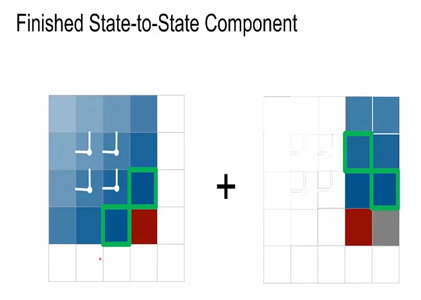
However, implementing the reverse stream is geometrically subtle. We cannot simply flip the scan order and reuse the same skew, because a naive application of the \(2 \times 1\) state-to-state kernel would read from future pixels and break autoregressiveness. To see this concretely, consider the toy configuration in the following figure.

Summarizing the logic in Figure 19.13:

• Naive reversal. With the standard skew, the reverse stream’s \(2 \times 1\) kernel is aligned so that one of its taps falls on the Right neighbor. From the perspective of the current diagonal \(d\), this neighbor belongs to diagonal \(d{+}1\) (the future). Using it would leak information from the future into the prediction.
• Causal shift. By skewing the reverse stream with an extra one-row downward offset, the geometric position of the future pixel is moved outside the kernel’s receptive field. The two taps of the \(2 \times 1\) kernel now sit entirely on blue cells that represent already-generated pixels from earlier diagonals. In other words, the kernel sees \((\mbox{past}, \mbox{past})\) instead of \((\mbox{past}, \mbox{future})\), forcing the reverse stream to aggregate information only from valid past context.

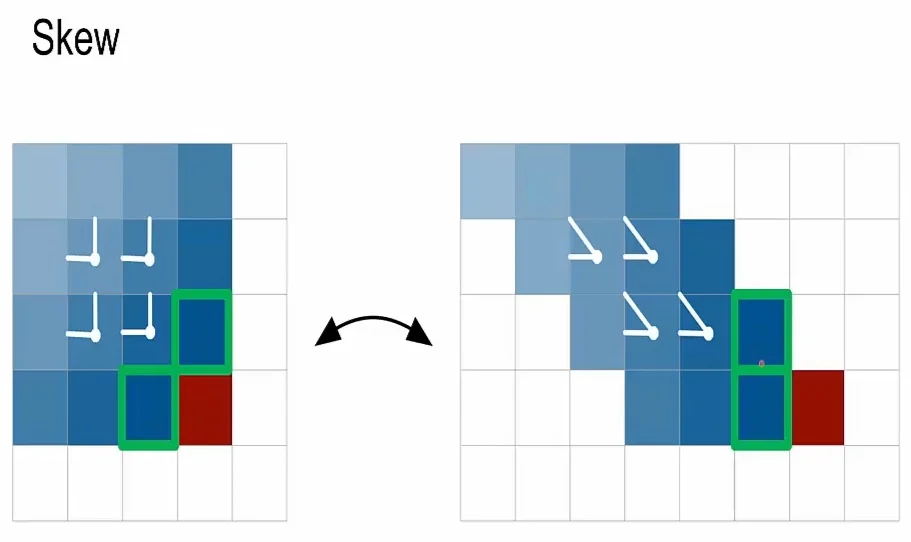
Merging the Streams After computing the hidden states for both directions, their outputs must be combined into a single feature map:

1.

Unskewing: Each stream’s output is first unskewed back to the original \(H \times W\) grid, reversing the row offsets.

2.

Shift correction (reverse stream only): The reverse stream’s output is shifted up by one row to undo the extra downward offset used to enforce causality, so that both streams are spatially aligned.

3.

Fusion: The aligned hidden maps are fused, typically by summation \[ \mathbf {h}^{\mathrm {diag}}(i,j) = \mathbf {h}^{\mathrm {fwd}}(i,j) + \mathbf {h}^{\mathrm {rev}}(i,j), \] or by concatenation followed by a \(1 \times 1\) projection. The resulting representation at each pixel \((i, j)\) encodes information from the entire past half-plane, with symmetric contributions from both sides of the image.

Why Diagonal BiLSTM is the Most Expressive Variant

• Global Context without Blind Spots: While the Row LSTM is limited to a triangular receptive field above the pixel (leaving valid ”past” pixels to the top-right unreachable), the Diagonal BiLSTM covers the entire available past. By combining the forward and reverse streams, every pixel \((i, j)\) can effectively aggregate information from all previously generated pixels \((r, c)\) where \(r+c < i+j\).
• Simultaneous Horizontal and Vertical Processing: Unlike the Row LSTM, which processes row-by-row and relies on stacking layers to slowly widen its receptive field, the Diagonal BiLSTM naturally processes both spatial dimensions at once. The skewing operation allows the \(2 \times 1\) kernel to capture vertical and horizontal neighbors simultaneously in a single layer, enabling the model to learn complex, long-range spatial dependencies more efficiently.

Residual Connections in PixelRNNs Training deep autoregressive models poses a significant challenge: gradients must propagate not only through the spatial recurrence (rows or diagonals) but also through the depth of many stacked layers. To enable the training of deep networks (e.g., 12 layers), PixelRNN wraps each LSTM layer in a residual block [206], allowing the model to learn incremental refinements while maintaining a direct path for gradient flow.

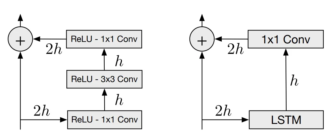
The Residual Bottleneck Design

The architecture defines a ”residual stream” with a fixed channel width of \( 2h \). This stream acts as the backbone of the network, carrying features from layer to layer. However, the internal hidden state of each LSTM layer has a smaller width of \( h \). This creates a bottleneck structure within each block (see the below figure, on its right side):

1.

Input (\(2h\)): The block receives a feature map \(\mathbf {x}\) with \(2h\) channels from the previous layer.

2.

LSTM Processing (\(h\)): The input is processed by the Row LSTM or Diagonal BiLSTM layer. Although the input-to-state convolution maps \(2h \to 4h\) (to compute the four gates), the resulting hidden state \(\mathbf {h}\) has only \(h\) channels.

3.

Output Projection (\(h \to 2h\)): To merge this state back into the residual stream, the hidden state \(\mathbf {h}\) is projected up using a \(1 \times 1\) convolution, restoring the dimension to \(2h\).

4.

Residual Addition: This projected output is added elementwise to the original input \(\mathbf {x}\).

\[ \mathbf {y} = \mathbf {x} + \mbox{Conv}_{1\times 1}(\mbox{LSTM}(\mathbf {x})) \]

This connection is between layers, distinct from the recurrent connections within a layer. It allows gradients to bypass the complex LSTM dynamics during backpropagation, stabilizing the learning process.

Looking Ahead With the residualized Row LSTM and Diagonal BiLSTM, PixelRNN achieves a receptive field that is both deep and spatially complete. The Diagonal BiLSTM, in particular, offers the most expressive spatial modeling by aggregating full diagonal contexts, though at the cost of higher computational complexity than the Row LSTM.

However, all variants discussed so far generate images at the original resolution pixel-by-pixel, which remains computationally expensive regardless of the variant. The primary limitation of single-scale models is not just speed, but their difficulty in capturing long-range global structure on large canvases. In the next section, we examine the Multi-Scale PixelRNN, which introduces a coarse-to-fine generation strategy. While this does not accelerate inference, it significantly improves global coherence and allows the model to scale effectively to higher-resolution images.

Multi-Scale PixelRNN

The Multi-Scale PixelRNN is a hierarchical extension of the standard PixelRNN framework designed to improve image coherence and scalability [458]. A single, full-resolution PixelRNN can in principle model the entire image distribution \(p(\mathbf {X}_{\mbox{high}})\) directly, but in practice, most of its capacity is spent on modeling very local correlations (textures, small edges), which dominate the likelihood loss. Gradients that encode global structure (overall shape, pose, layout) are diluted across millions of pixels, so the network may fail to fully exploit long-range dependencies.

Multi-Scale PixelRNN addresses this by making the generation explicitly coarse-to-fine. The image distribution is factorized as \[ p(\mathbf {X}_{\mbox{high}}) = p(\mathbf {X}_{\mbox{coarse}})\; p(\mathbf {X}_{\mbox{high}} \mid \mathbf {X}_{\mbox{coarse}}), \] where a low-resolution model is responsible for the global “plan”, and a second, conditional model fills in high-resolution details given that plan.

High-Level Architecture and Intuition The architecture consists of two PixelRNN networks trained jointly end-to-end to maximize the log-likelihood of the full-resolution images:

1.

Stage 1 (Coarse, Unconditional): A small PixelRNN operates on a downsampled grid \(\mathbf {X}_{\mbox{coarse}} \in \mathbb {R}^{3 \times s \times s}\) (typically \(s = n/2\)). It is an unconditional autoregressive model: given no additional input, it generates a low-resolution thumbnail pixel by pixel (and channel by channel) using the same machinery as the single-scale Row LSTM or Diagonal BiLSTM. Because the grid is small, even a shallow stack of recurrent layers already has a very large effective receptive field, so Stage 1 can devote its capacity almost entirely to modeling global layout, object placement, and coarse color composition.

2.

Stage 2 (Fine, Conditional): A full-resolution PixelRNN generates the final image \(\mathbf {X}_{\mbox{high}} \in \mathbb {R}^{3 \times n \times n}\) conditioned on \(\mathbf {X}_{\mbox{coarse}}\). Architecturally it looks like a standard PixelRNN on the \(n \times n\) grid (same masked convolutions, same recurrent geometry). The only change is that every LSTM layer receives an additional spatial bias derived from the coarse image. This stage therefore concentrates its capacity on modeling residual structure: fine textures, sharp edges, and local variations, while being guided by the global plan coming from Stage 1 rather than having to infer that plan from scratch.

Conditioning via Upsampling and Spatial Bias Fields The core design question is how to inject the coarse image \(\mathbf {X}_{\mbox{coarse}}\) into the high-resolution PixelRNN without breaking causality. PixelRNN does this by turning the coarse image into a spatially varying bias field that is fixed for the entire generation of \(\mathbf {X}_{\mbox{high}}\).

1.

Upsampling Network (Global Context Features). The generated coarse image \(\mathbf {X}_{\mbox{coarse}}\) is first passed through a convolutional decoder (a stack of deconvolution / transpose-convolution layers; see §15.2). This upsamples it to a dense feature map \(\mathbf {C}_{\mbox{up}} \in \mathbb {R}^{c \times n \times n}\). Conceptually, each coarse pixel now “paints” a soft template over its corresponding block in the high-resolution grid, encoding rough foreground/background regions, large edges, color tendencies, and other low-frequency information.

2.

Injecting the Bias into Each LSTM Layer. For each LSTM layer in Stage 2, this upsampled map is injected into the input-to-state path. Using the notation from the Row / Diagonal LSTM sections, the gate pre-activations at index \(t\) (row or diagonal) are \begin {equation} [\mathbf {o}_t, \mathbf {f}_t, \mathbf {i}_t, \mathbf {g}_t] = \underbrace {\mathbf {K}^{is} \ast \mathbf {x}_t}_{\mbox{Current local input}} \;+\; \underbrace {\mathbf {K}^{\mbox{cond}} \ast \mathbf {C}_{\mbox{up}}}_{\mbox{Global context bias}} \;+\; \underbrace {\mathbf {K}^{ss} \ast \mathbf {h}_{t-1}}_{\mbox{Recurrent state}}. \label {eq:chapter19_multiscale_gates} \end {equation} Here

• \(\mathbf {x}_t\) is the masked local input at step \(t\) (current row or diagonal), and \(\mathbf {K}^{is}\) is the usual input-to-state convolution kernel.
• \(\mathbf {h}_{t-1}\) is the previous hidden map, and \(\mathbf {K}^{ss}\) is the state-to-state kernel (e.g., a \(2 \times 1\) convolution in a Diagonal BiLSTM).
• \(\mathbf {K}^{\mbox{cond}}\) is an unmasked \(1 \times 1\) convolution that maps \(\mathbf {C}_{\mbox{up}} \in \mathbb {R}^{c \times n \times n}\) to \(\mathbb {R}^{4h \times n \times n}\), producing one \(h\)-dimensional bias vector per gate and per pixel location.

For a given image and a given layer, the tensor \(\mathbf {K}^{\mbox{cond}} \ast \mathbf {C}_{\mbox{up}}\) is computed once and reused for all steps \(t\). It is fixed in time but varies in space, so it acts like a learned prior field saying, for example, “this region is likely background, close the input gate” or “this region lies on an object boundary, keep gates open and propagate detail”. Different layers have different \(\mathbf {K}^{\mbox{cond}}\), so the coarse context can influence early, mid-level, and deep features in different ways.

Why the Conditioning is Causal (No “Cheating”) At first glance, adding a dense global map \(\mathbf {C}_{\mbox{up}}\) to every gate seems to violate the autoregressive constraint. If the network can see the entire coarse map at position \((0,0)\), isn’t it looking into the future?

The answer is no. The conditional model \(p(\mathbf {X}_{\mbox{high}} \mid \mathbf {X}_{\mbox{coarse}})\) remains perfectly causal because we must distinguish between the conditioning signal (which is fixed) and the target pixels (which are being generated).

• Stage-wise Factorization (The ”Class Label” Analogy). The joint distribution is defined as: \[ p(\mathbf {X}_{\mbox{high}}, \mathbf {X}_{\mbox{coarse}}) = p(\mathbf {X}_{\mbox{coarse}})\; p(\mathbf {X}_{\mbox{high}} \mid \mathbf {X}_{\mbox{coarse}}). \]

  During sampling, Stage 1 generates \(\mathbf {X}_{\mbox{coarse}}\) completely. By the time Stage 2 begins, \(\mathbf {X}_{\mbox{coarse}}\) is fully observed and fixed. From the perspective of the high-resolution generator, the coarse image acts exactly like a class label or a text prompt. Just as knowing the label ”Dog” doesn’t tell you exactly what the pixel at \((50, 50)\) looks like, knowing the coarse thumbnail doesn’t reveal the specific high-frequency details of the future pixels.

• Per-pixel Dependencies and Masking. To see why the math holds, let’s look at the information flow for a single high-resolution pixel \(x_t\) at step \(t\). The gate inputs are: \[ \mbox{Gates}_t = \underbrace {\mathbf {K}^{is} \ast \mathbf {x}_t}_{\mbox{Masked High-Res Input}} \;+\; \underbrace {\mathbf {K}^{ss} \ast \mathbf {h}_{t-1}}_{\mbox{Causal Recurrent State}} \;+\; \underbrace {\mathbf {K}^{\mbox{cond}} \ast \mathbf {C}_{\mbox{up}}}_{\mbox{Global Context}}. \]

  • The first two terms depend on \(\mathbf {x}_t\) and \(\mathbf {h}_{t-1}\). These are strictly governed by Mask A/B and the LSTM’s causal direction. They ensure the model cannot see high-resolution pixels \(x_{>t}\) (the true future).
  • The third term depends on \(\mathbf {C}_{\mbox{up}}\). Since \(\mathbf {X}_{\mbox{coarse}}\) contains no information about the specific high-frequency noise or texture of \(\mathbf {X}_{\mbox{high}}\), reading it does not leak the value of \(x_{>t}\).
• Conditional Distribution, Not Interpolation. Because the coarse image is a lossy summary (e.g., a \(32 \times 32\) grid representing a \(64 \times 64\) image), it cannot define the high-resolution image deterministically. The Stage 2 network must still use its autoregressive masking to model the remaining uncertainty and generate the fine details pixel-by-pixel.

Why Multi-Scale Helps This hierarchical design improves modeling in several ways:

• Global Structure: On the small \(s \times s\) grid, each recurrent layer has a receptive field that quickly covers the entire image, so Stage 1 can easily learn coherent global shapes and layouts (e.g., the outline of a digit or the rough structure of a face). A single full-resolution PixelRNN would need to be much deeper to achieve the same coverage.
• Separation of Concerns: By offloading long-range planning to the coarse stage, the fine stage can dedicate its capacity to local textures and sharp details. Gradients for global structure flow primarily through Stage 1, rather than being overwhelmed by local-error terms at the pixel level.
• Scalability and Sample Quality: Although Multi-Scale PixelRNN does not fundamentally speed up inference (pixels in \(\mathbf {X}_{\mbox{high}}\) are still generated one by one), it uses parameters more effectively. Empirically, this leads to sharper and more coherent samples on larger images than a single-scale PixelRNN with comparable capacity [458].

Results and Qualitative Samples

The original PixelRNN models were evaluated on standard image generation benchmarks, including CIFAR-10 and downsampled ImageNet at \(32 \times 32\) resolution. At the time of their release, the Row LSTM, Diagonal BiLSTM, and Multi-Scale PixelRNN variants achieved state-of-the-art negative log-likelihood (NLL) scores, significantly outperforming earlier autoregressive baselines.

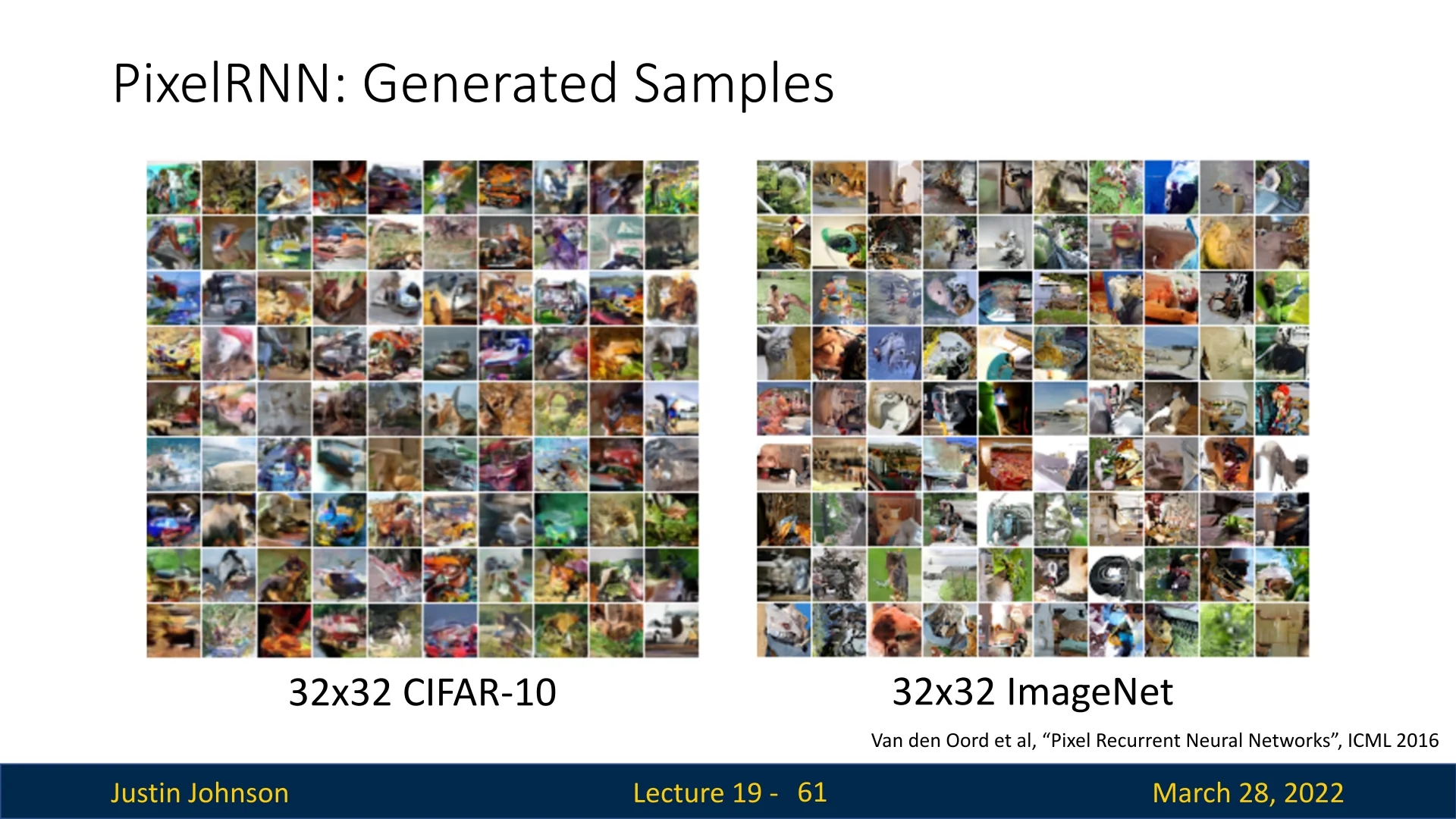
Qualitatively, the samples (Figure 19.17) illustrate the distinct characteristics of discrete autoregressive modeling:

• Sharp Local Structure: A key strength of PixelRNN is the ability to generate crisp, non-blurry textures and edges. Because the model uses a discrete 256-way softmax for pixel values (rather than a continuous Gaussian or L2 loss), it avoids the averaging effect common in Variational Autoencoders (VAEs). It can predict multi-modal distributions (e.g., ”this pixel is either black or white”) rather than producing a blurry gray average.
• Emergent Global Layout: Despite the difficulty of modeling long-range dependencies, the Diagonal BiLSTM and Multi-Scale variants capture coarse object shapes and scene layouts surprisingly well. The authors noted that models trained on ImageNet, which contains more distinct object classes, tended to learn better global structures than those trained on CIFAR-10.
• Implicit Class Priors: Although trained without class labels, the samples often exhibit semantic consistency, producing recognizable ”dream-like” approximations of animals, vehicles, and landscapes.

However, these results also highlight the inherent trade-offs of early autoregressive approaches:

• Slow Sequential Generation: The most significant drawback is inference speed. Generating an image requires passing through the network \(N^2\) times (once per pixel), making the process computationally expensive and difficult to scale to high resolutions (e.g., HD video).

• Dominance of Local Statistics: The likelihood objective function is often dominated by high-frequency details (local textures) rather than high-level semantics. As a result, the model may generate perfectly sharp textures that form incoherent objects—a ”perfect texture, wrong geometry” phenomenon. The Multi-Scale PixelRNN attempts to mitigate this by enforcing a global plan, but the tension between local detail and global structure remains a challenge.

These limitations—particularly the slow sampling time—motivate the exploration of parallelizable architectures (like PixelCNN) and alternative generative paradigms such as VAEs, GANs, and Diffusion models, which we explore in the following sections.

Enrichment 19.3.4.1: Beyond PixelRNN: Advanced Autoregressive Variants

The PixelRNN family helped catalyze a wave of progress in autoregressive image modeling. Although the original LSTM-based architectures are rarely used in modern systems, the core ideas they exemplify—strict autoregressive factorization, masked computation, and careful handling of spatial dependencies—directly informed a number of more scalable and performant successors.

Gated PixelCNN The original PixelCNN employed stacks of masked convolutions with simple pointwise nonlinearities (e.g., ReLU), which limited its expressivity and retained a ”blind spot” in the receptive field geometry [458]. Gated PixelCNN augments this design with:

• A gated activation unit that replaces ReLU with a multiplicative interaction: \[ \mathbf {y} = \tanh (\mathbf {W}_f * \mathbf {x}) \odot \sigma (\mathbf {W}_g * \mathbf {x}), \] where \(\sigma \) is the logistic sigmoid and \(*\) denotes a masked convolution.
• A decomposition into vertical and horizontal stacks of masked convolutions, with carefully designed masks so that the union of the two stacks covers the entire causal past of each pixel without leaving blind spots.

The gating provides richer, input-dependent modulation than a plain ReLU, and the vertical–horizontal decomposition fixes the receptive-field gaps of the original PixelCNN while preserving fully convolutional computation. Empirically, this yields sharper samples and better log-likelihoods than the baseline PixelCNN.

PixelCNN++ PixelCNN++ [544] further improves convolutional autoregressive models through a set of architectural and likelihood-design changes. Key contributions include:

• Replacing the discrete softmax over 256 intensity values with a discretized logistic mixture likelihood, which better matches the heavy-tailed, multi-modal statistics of natural image intensities.
• Using residual blocks, downsampling and upsampling stages, and short skip connections to ease optimization and expand the effective receptive field without requiring extremely deep purely local stacks.
• Applying regularization (e.g., dropout) and architectural tuning that together yield state-of-the-art negative log-likelihoods on benchmarks such as CIFAR-10, while remaining a purely likelihood-based model.

PixelCNN++ is often taken as the ”mature” convolutional pixel model: it retains exact likelihood and autoregressive structure but is more robust and expressive than earlier variants.

ImageGPT ImageGPT [84] lifts the autoregressive idea into the Transformer era by treating images as sequences of discrete tokens and applying a GPT-style Transformer architecture. The pipeline is conceptually simple:

• An image is tokenized (e.g., as a raster-ordered sequence of color values or codebook indices), forming a 1D sequence analogous to a sentence.
• A causal Transformer (closely related to GPT-2) models the distribution over the next token given all previous ones, using self-attention instead of convolutions.
• The model is trained with the same maximum-likelihood objective as language GPT; the learned representations can then be transferred to downstream tasks such as classification via linear probes or fine-tuning.

ImageGPT demonstrated that large-scale autoregressive pretraining on pixels can yield competitive performance on supervised vision benchmarks. However, the sequential nature of sampling remains: generating a \(64 \times 64\) or \(128 \times 128\) image requires thousands of autoregressive steps, and self-attention introduces quadratic cost in the sequence length.

Taken together, these successors illustrate the long tail of the PixelRNN lineage: they preserve the core autoregressive factorization but progressively replace LSTMs with more scalable architectures (deep residual CNNs, then Transformers) to better exploit modern compute budgets.

Looking Ahead: From Autoregressive Models to VAEs Autoregressive models such as PixelCNN, PixelRNN, and ImageGPT provide one of the most principled approaches to generative modeling in vision. Their defining property is that they represent the joint distribution over all pixels via an exact factorization: \[ p(\mathbf {x}) = \prod _{i=1}^{H \times W} p(x_i \mid x_{<i}), \] where \(x_i\) is the \(i\)-th pixel (or channel) in some fixed ordering, and \(x_{<i}\) denotes all preceding pixels. For any fully observed image, this factorization yields a tractable, normalized log-likelihood: every conditional term can be evaluated exactly by providing the ground-truth values of \(x_{<i}\) as inputs (teacher forcing).

During training, we maximize the log-likelihood on the training set. At evaluation time, we compute the same objective on unseen test images: since the entire image is known, every conditional \(p(x_i \mid x_{<i})\) is obtained in one forward pass, and their product (or sum of logs) gives an exact density value per image. This makes autoregressive models particularly attractive when:

• We care about calibrated density estimation (e.g., bits-per-dimension comparisons).
• We want a principled score for tasks such as anomaly detection or uncertainty estimation.

In contrast, GANs do not define a normalized likelihood at all, and VAEs optimize a variational lower bound (ELBO) that only approximates the true log-likelihood.

However, these strengths come with serious practical drawbacks:

• Slow sampling. Because pixels (or tokens) are generated one at a time, sampling is inherently sequential. Even with efficient implementations, generating a moderate-resolution image can require thousands of autoregressive steps; each step depends on all previous ones.
• Scaling with resolution. To model long-range dependencies at higher resolutions, autoregressive models must either become very deep or very wide, increasing memory and compute. Transformer-based variants also incur \(\mathcal {O}(T^2)\) attention cost in the sequence length \(T = H \times W\).
• Architectural rigidity. LSTM-based models like Row LSTM and Diagonal BiLSTM are typically designed and trained for a fixed spatial resolution and a specific scan geometry. Adapting them to arbitrary resolutions is non-trivial.
• Complex conditional extensions. Conditioning on labels, low-resolution images, or other modalities usually requires additional networks and masking logic—as in Multi-Scale PixelRNN—further increasing architectural complexity.

These limitations motivate latent variable models such as Variational Autoencoders (VAEs). VAEs trade exact, per-pixel autoregression for:

• A global, low-dimensional latent representation that captures coarse structure in a single vector or feature map.
• Feedforward sampling: once a latent code is drawn, an image is produced in a single pass through the decoder, enabling much faster generation at test time.
• A principled probabilistic training objective (the ELBO) that provides a lower bound on log-likelihood while allowing parallel computation over pixels.

In the next section, we will introduce VAEs, show how they define a generative model via latent variables, and compare their strengths and weaknesses against the autoregressive models discussed so far.

19.4 Variational Autoencoders (VAEs)

To address autoregressive models shortcomings, we now turn to a different family of models: Variational Autoencoders (VAEs). Unlike autoregressive models, VAEs define a joint density over observed data \(\mathbf {x}\) and latent variables \(\mathbf {z}\), but this density is typically intractable to compute or optimize directly. Instead, VAEs derive and maximize a tractable lower bound on the marginal log-likelihood of the data. By optimizing this lower bound (the ELBO), we hope to increase the true likelihood as well — even if it cannot be evaluated exactly.

Before diving into the variational formulation, we briefly introduce standard (non-variational) autoencoders to set the stage.

19.4.1 Regular (Non-Variational) Autoencoders

Autoencoders are an unsupervised learning approach designed to extract useful features (latent codes) from raw data — in our case, images. The architecture consists of two main components:

• An encoder \( f_{\theta }(\mathbf {x}) \): maps the input image \( \mathbf {x} \) to a lower-dimensional feature representation \( \mathbf {z} \).
• A decoder \( g_{\phi }(\mathbf {z}) \): attempts to reconstruct the original input \( \hat {\mathbf {x}} = g_{\phi }(f_{\theta }(\mathbf {x})) \).

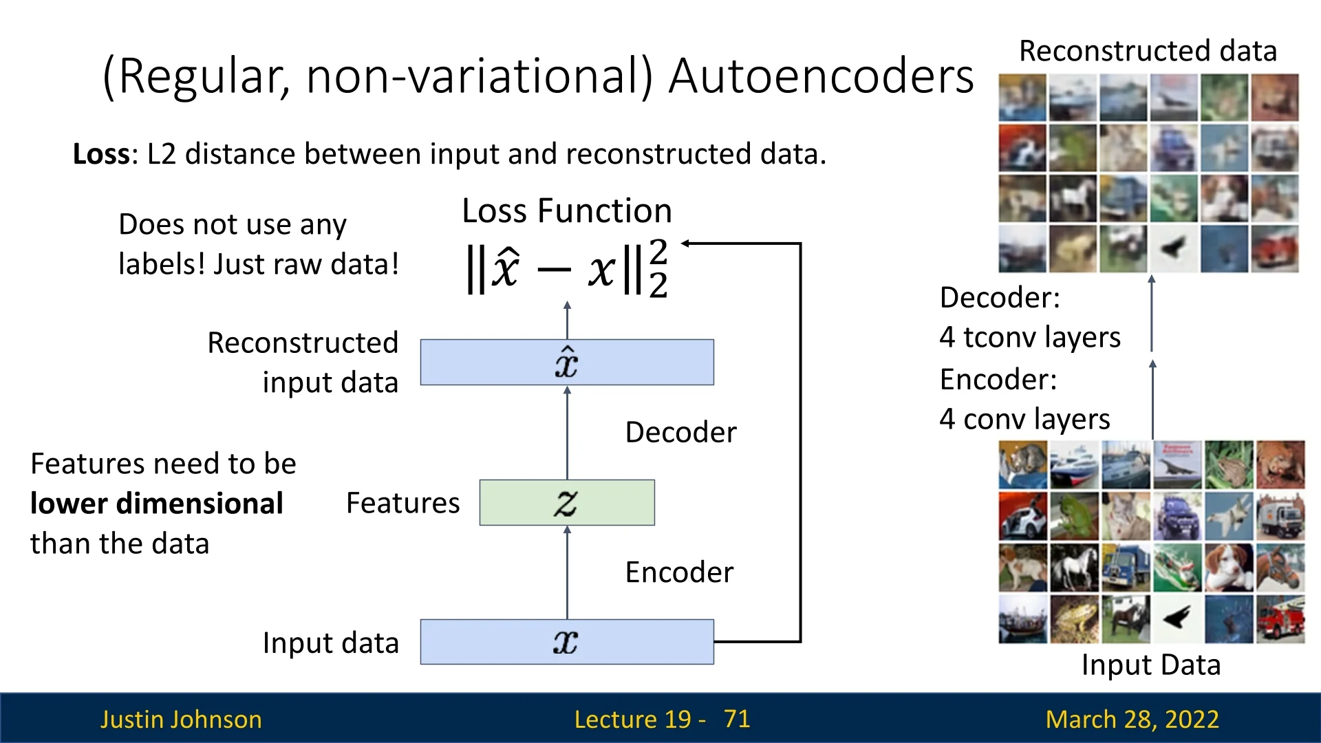
Training is unsupervised: we minimize the reconstruction loss, which is typically the squared Euclidean distance (L2 norm): \[ \mathcal {L}_{\mbox{AE}}(\mathbf {x}) = \| \mathbf {x} - g_{\phi }(f_{\theta }(\mathbf {x})) \|^2 \] Why L2? In the probabilistic view (which VAEs rely on), minimizing the squared error is equivalent to maximizing the log-likelihood of the data under a Gaussian distribution assumption (\(p(\mathbf {x}|\mathbf {z}) = \mathcal {N}(\mathbf {x}; \hat {\mathbf {x}}, \sigma ^2\mathbf {I})\)). While L1 loss is sometimes used to encourage sharper edges (as it corresponds to a Laplacian distribution), L2 is the standard choice for continuous data as it creates stable gradients and naturally fits the Gaussian generative model structure. The encoder must compress the input into a bottleneck representation \( \mathbf {z} \), forcing it to retain only the most salient features.

Usage in Transfer Learning After training, the decoder is often discarded. The encoder can be repurposed to extract features for downstream tasks (e.g., classification, segmentation), often with fine-tuning on a small labeled dataset.

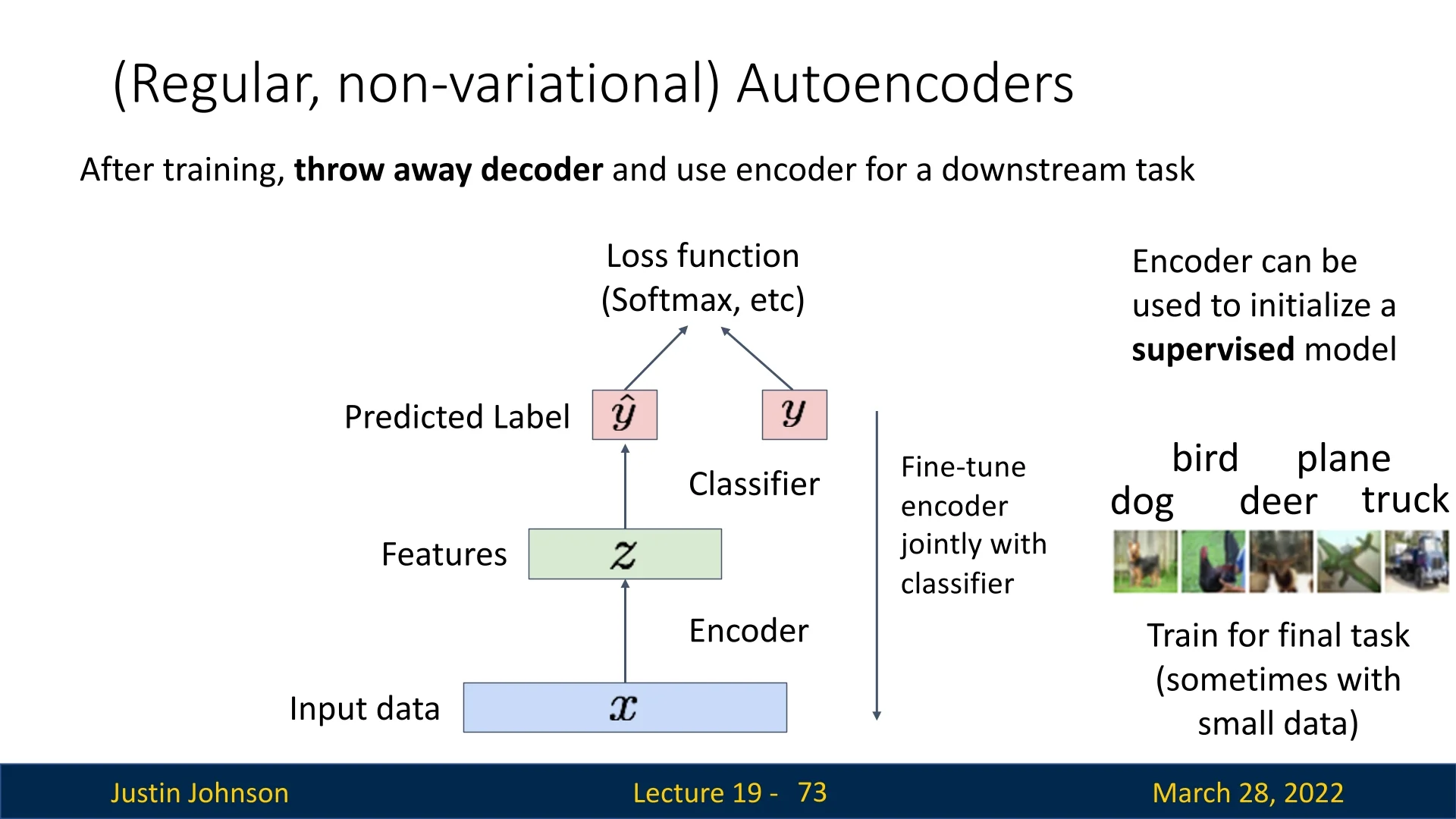
Architecture Patterns Autoencoders typically follow an encoder-decoder architecture, where:

• The encoder downsamples the input using strided convolutions, pooling layers, or other operations to produce a latent code \( \mathbf {z} \).
• The decoder upsamples \( \mathbf {z} \) using transposed convolutions, interpolation layers, or learned upsampling blocks to recover the original input resolution.

Importantly, there are no strict architectural requirements for either component: both the encoder and decoder can be implemented using convolutional neural networks (CNNs) with ReLU activations, Transformer blocks, MLPs, or any other differentiable function class. While the encoder and decoder often mirror each other structurally, this is not required and often depends on the task and data modality.

Limitations of Vanilla Autoencoders While intuitive and easy to implement, regular autoencoders suffer from two significant drawbacks:

1.

Limited generative capability: These models are not probabilistic — they learn deterministic mappings and cannot generate new samples from a learned distribution.

2.

Limited success in practice: Despite their potential, regular autoencoders rarely achieve state-of-the-art results in unsupervised representation learning or generative modeling.

To address these limitations, we now turn to a probabilistic extension: the Variational Autoencoder (VAE) — a model that will hopefully won’t only learn compact and meaningful latent representations but will also enable sampling of novel, coherent outputs from the learned distribution.

19.4.2 Introducing the VAE

Core Goals Variational Autoencoders (VAEs) aim to unify representation learning with generative modeling in a single probabilistic framework [292]. Their primary objectives are:

1.

Representation: Learn a low-dimensional latent representation \( \mathbf {z} \) from high-dimensional input data \( \mathbf {x} \) (e.g., images), capturing semantic factors like shape, pose, or object identity.

2.

Generation: Define a generative process \( p_\theta (\mathbf {x} \mid \mathbf {z}) \) that allows sampling new, synthetic data by drawing random codes from a prior \( p(\mathbf {z}) \).

Why a Latent Variable Model? We assume that the observed data \( \mathbf {x} \in \mathbb {R}^{D} \) is generated by an underlying, lower-dimensional set of unobserved factors \( \mathbf {z} \in \mathbb {R}^{n} \) (where \( n \ll D \)). Although we cannot see \( \mathbf {z} \), we model the generation process explicitly:

• 1. Sample a latent code: \( \mathbf {z} \sim p(\mathbf {z}) \). We typically choose the prior to be a standard multivariate Gaussian: \[ p(\mathbf {z}) = \mathcal {N}(\mathbf {0}, \mathbf {I}). \] This choice is widely adopted for several theoretical and practical reasons:

  • Tractability: Sampling is trivial, and the log-density is known in closed form, simplifying the training objective.
  • Smoothness and Isotropy: The standard Gaussian is isotropic (rotationally symmetric), meaning no direction in the latent space is privileged. This encourages the model to distribute information smoothly, avoiding ”holes” or discontinuous regions.
  • Compactness in High Dimensions: In high-dimensional spaces, the mass of a standard Gaussian concentrates in a ”typical set” (a thin shell) around the origin. This ensures that valid latent codes lie within a bounded region, making it easy to sample new codes that the decoder can interpret, even if they were never seen during training.
  • Semantic Interpolation: A well-trained VAE maps semantically similar data points to nearby locations in \( \mathbf {z} \)-space. As a result, linear interpolation between two latent vectors typically yields smooth semantic transitions in the output (e.g., morphing a digit ’1’ into a ’7’) rather than chaotic noise.

• 2. Generate the data: \( \mathbf {x} \sim p_\theta (\mathbf {x} \mid \mathbf {z}) \). The decoder (or generative network) takes \( \mathbf {z} \) as input and outputs the parameters of a probability distribution over the data.

  • For binary data (e.g., MNIST), the decoder might output Bernoulli probabilities for each pixel.
  • For real-valued data (e.g., natural images), it typically outputs the mean and variance of a Gaussian or the parameters of a discretized logistic mixture for each pixel.

The Inference Problem The generative story above describes how to create data from latents. However, to learn meaningful representations, we need the reverse mapping: given an image \( \mathbf {x} \), what is its latent code \( \mathbf {z} \)? This requires computing the posterior \( p_\theta (\mathbf {z} \mid \mathbf {x}) \), which is generally intractable. The ”Variational” in VAE comes from introducing an inference model (encoder) \( q_\phi (\mathbf {z} \mid \mathbf {x}) \) to approximate this posterior, a process we detail in the next section.

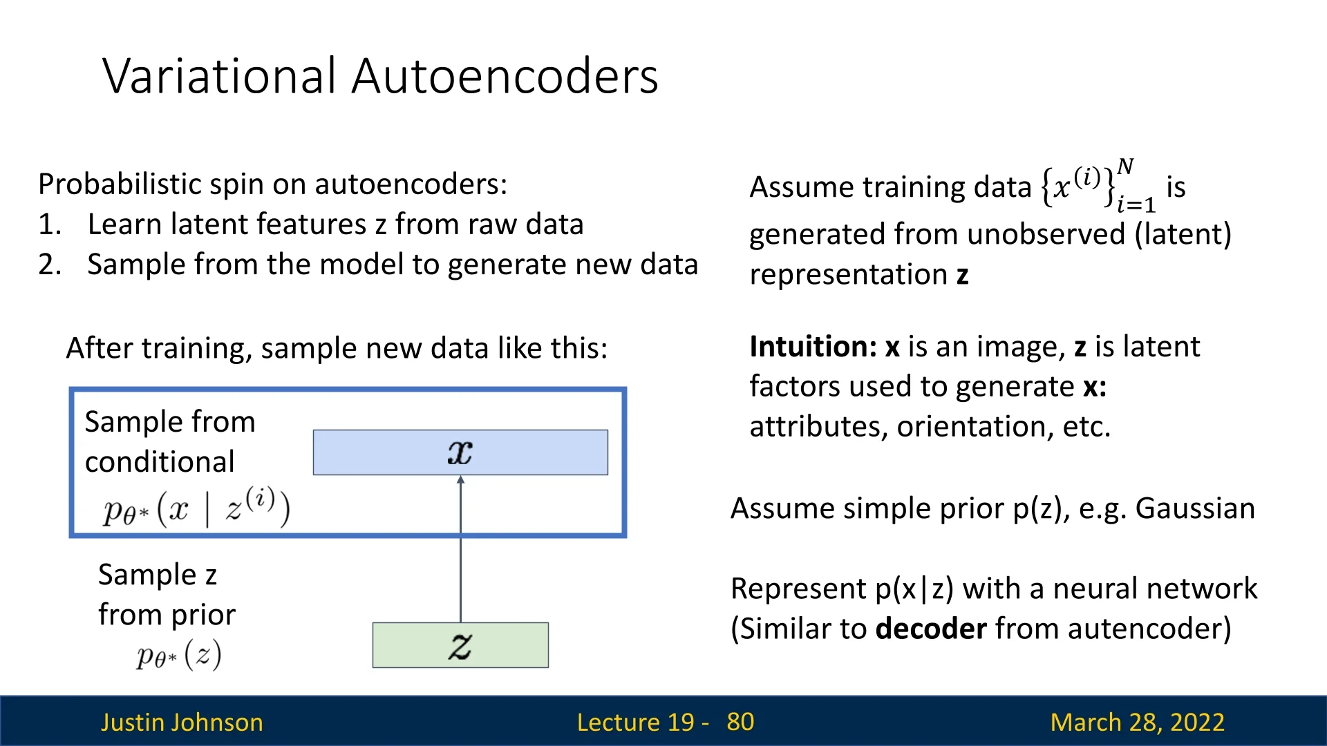
Probabilistic Decoder Unlike standard autoencoders, which reconstruct a deterministic output image, VAEs treat the decoder as a conditional distribution. For example, we assume that: \[ p_\theta (\mathbf {x} \mid \mathbf {z}) = \mathcal {N}\big (\boldsymbol {\mu }_\theta (\mathbf {z}), \operatorname {diag}(\boldsymbol {\sigma }^2_\theta (\mathbf {z}))\big ) \] That is, the decoder outputs the parameters (mean and variance) of a Gaussian distribution over all pixels. This enables stochastic sampling of images given a latent code.

• \( \boldsymbol {\mu }_\theta (\mathbf {z}) \in \mathbb {R}^{D} \): predicted mean per pixel.
• \( \boldsymbol {\sigma }^2_\theta (\mathbf {z}) \in \mathbb {R}^{D} \): predicted variance per pixel.

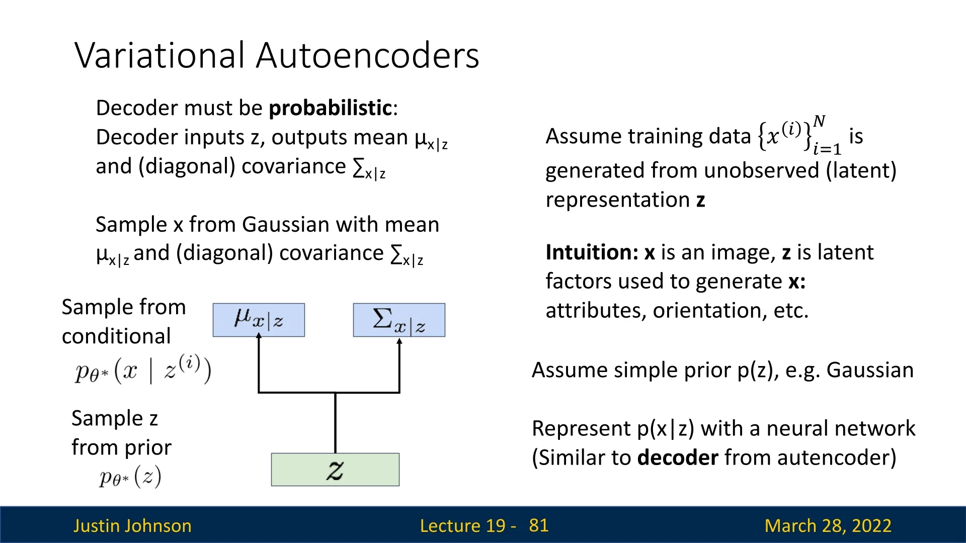
Why Not a Full Covariance Decoder? In principle, if we view the decoder as a conditional density model, we could allow it to predict a full Gaussian covariance matrix \(\boldsymbol {\Sigma }_\theta (\mathbf {z}) \in \mathbb {R}^{D \times D}\) for each latent code \(\mathbf {z}\), capturing all possible pixel-wise correlations: \begin {equation} p_\theta (\mathbf {x} \mid \mathbf {z}) = \mathcal {N}\bigl (\boldsymbol {\mu }_\theta (\mathbf {z}), \boldsymbol {\Sigma }_\theta (\mathbf {z})\bigr ), \label {eq:chapter19_vae_fullcov_decoder} \end {equation} where \(D = H \times W \times C\) is the total number of dimensions (pixels \(\times \) channels). A full covariance matrix would allow the decoder to explicitly model complex dependencies, such as ”if pixel A is red, pixel B must be red” or ”if there is an edge at A, there must be a continuation at B”.

However, this is computationally intractable for any realistic image size:

• Parameter Explosion: A modest \(512 \times 512\) grayscale image has \(D \approx 2.6 \times 10^5\) pixels. A full covariance matrix \(\boldsymbol {\Sigma }_\theta (\mathbf {z})\) contains \(D^2 \approx 6.9 \times 10^{10}\) entries. The decoder would need to output billions of values for every single image.
• Computational Cost: Evaluating the Gaussian log-likelihood requires computing the determinant \(\det (\boldsymbol {\Sigma }_\theta )\) and the inverse \(\boldsymbol {\Sigma }_\theta ^{-1}\). The cost of these operations scales cubically, \(O(D^3)\), which is impossible for \(D > 10^4\) in deep learning loops.

The Diagonal Assumption and Conditional Independence To sidestep this explosion, VAEs typically assume that the pixels are conditionally independent given the latent code \(\mathbf {z}\). This enforces a diagonal structure on the covariance matrix, \(\boldsymbol {\Sigma }_\theta (\mathbf {z}) = \mbox{diag}(\boldsymbol {\sigma }^2_\theta (\mathbf {z}))\), reducing the likelihood to a product of independent terms: \begin {equation} p_\theta (\mathbf {x} \mid \mathbf {z}) = \prod _{i=1}^{D} \mathcal {N}\bigl (x_i \mid \mu _i(\mathbf {z}), \sigma _i^2(\mathbf {z})\bigr ). \label {eq:chapter19_vae_diag_decoder} \end {equation}

This assumption drastically simplifies computation:

• The number of decoder outputs drops from \(O(D^2)\) to \(O(D)\) (just a mean and variance per pixel).
• The log-likelihood computation becomes a simple sum over pixels, parallelizable on GPUs.
• If we fix the variance \(\sigma _i^2(\mathbf {z}) = \sigma ^2\) (constant), maximizing the log-likelihood is mathematically equivalent to minimizing the \(\ell _2\) reconstruction loss (Mean Squared Error), \(\|\mathbf {x} - \boldsymbol {\mu }_\theta (\mathbf {z})\|^2\).

The Trade-Off: Blurriness vs. Autoregressive Sharpness While efficient, the conditional independence assumption introduces a critical limitation compared to the autoregressive models (like PixelRNN/CNN) discussed earlier.

• Missing Local Correlations: In an autoregressive model, the probability of a pixel depends explicitly on its neighbors: \(p(x_i \mid x_{<i})\). This allows the model to make sharp, multimodal decisions (e.g., ”the neighbor is black, so this pixel must be black to continue the line”). In a diagonal VAE decoder, \(x_i\) depends only on \(\mathbf {z}\). The decoder cannot explicitly look at neighbor \(x_{i-1}\) to decide \(x_i\). All correlation must be ”baked in” to the latent code \(\mathbf {z}\). If \(\mathbf {z}\) fails to capture the exact, pixel-perfect alignment of an edge (which is difficult due to the compression bottleneck), the decoder must hedge its bets.

• The ”Average Face” Effect (Blurriness): Consider modeling a sharp edge that could validly be at position \(x\) or \(x+1\) depending on slight variations in pose.

  • An autoregressive model captures a multimodal distribution: it puts high probability on ”edge at \(x\)” OR ”edge at \(x+1\)”, generating one sharp outcome.
  • A diagonal Gaussian decoder is unimodal. Faced with uncertainty about the exact edge location, minimizing the MSE forces the model to predict the mean of all possible edge positions. The mathematical average of ”sharp edge at \(x\)” and ”sharp edge at \(x+1\)” is a blurry edge smeared across both positions.

Consequently, VAEs often produce images that capture global structure (face, glasses, orientation) correctly due to \(\mathbf {z}\), but suffer from distinct blurriness in fine details (hair texture, eyes) where local correlations are lost to averaging.

Marginal Likelihood: What We Want to Optimize Given a dataset \( \mathcal {D} = \{\mathbf {x}^{(i)}\}_{i=1}^N \), our primary goal is to learn a generative model \( p_\theta (\mathbf {x}) \) that assigns high probability to the real data. In a VAE, we define this model using a latent-variable generative process:

• The Prior (Latent Space): We assume the data is generated from unseen latent factors \( \mathbf {z} \). We place a simple prior on these factors, typically a standard Gaussian \( \mathbf {z} \sim p(\mathbf {z}) = \mathcal {N}(\mathbf {0}, \mathbf {I}) \).
• The Decoder (Likelihood): Given a latent code \( \mathbf {z} \), a neural network (the decoder, parameterized by \( \theta \)) generates the data. This defines the conditional likelihood \( p_\theta (\mathbf {x} \mid \mathbf {z}) \).

To train this model, we want to maximize the marginal likelihood of the observed data. This is obtained by integrating out the latent variable: \[ p_\theta (\mathbf {x}) = \int p_\theta (\mathbf {x}, \mathbf {z}) \, d\mathbf {z} = \int p_\theta (\mathbf {x} \mid \mathbf {z}) \, p(\mathbf {z}) \, d\mathbf {z}. \]

The Intractability Problem. Evaluating this integral is computationally impossible for two main reasons:

1.

High Dimensionality: The latent space \( \mathbf {z} \) is high-dimensional (e.g., \(n=512\)), meaning the volume of the space is massive.

2.

Sparseness: The vast majority of random \( \mathbf {z} \) samples from the prior will decode to static noise (\( p_\theta (\mathbf {x} \mid \mathbf {z}) \approx 0 \)). The valid codes that actually look like our specific image \( \mathbf {x} \) occupy a tiny, unknown region. Finding them via naive sampling is like searching for a needle in a hyperspace haystack.

Consequently, we cannot compute \( p_\theta (\mathbf {x}) \) or its gradient directly.

The Solution: Amortized Inference. Since we cannot search the entire space, we need a mechanism to directly identify the relevant latent codes for a given image. Ideally, we would use the true posterior \( p_\theta (\mathbf {z} \mid \mathbf {x}) \), which tells us exactly which \( \mathbf {z} \)’s are likely given \( \mathbf {x} \). However, calculating this posterior via Bayes’ rule is circular—it requires dividing by the intractable marginal \( p_\theta (\mathbf {x}) \).

To break this cycle, VAEs introduce a second network: the Encoder (or inference network), parameterized by \( \phi \). \[ q_\phi (\mathbf {z} \mid \mathbf {x}) \approx p_\theta (\mathbf {z} \mid \mathbf {x}) \] Crucially, the encoder does not output a single latent vector \( \mathbf {z} \). Instead, given an input \( \mathbf {x} \), it outputs the parameters of a probability distribution (e.g., mean \( \boldsymbol {\mu } \) and variance \( \boldsymbol {\sigma }^2 \)) from which we can sample.

• This defines a density \( q_\phi (\mathbf {z} \mid \mathbf {x}) \) that is non-zero everywhere (full support).
• It allows us to focus our sampling on the tiny region of latent space that matters for \( \mathbf {x} \).

Training VAEs and Developing the ELBO

Deriving the Tractable Objective We aim to maximize the log-likelihood \( \log p_\theta (\mathbf {x}) \). Although we cannot compute it directly, we can derive a valid lower bound using our approximate posterior \( q_\phi \).

We start with the definition of conditional probability, \( p_\theta (\mathbf {z} \mid \mathbf {x}) = p_\theta (\mathbf {x}, \mathbf {z}) / p_\theta (\mathbf {x}) \). Rearranging this gives us a useful identity for the marginal likelihood: \[ p_\theta (\mathbf {x}) = \frac {p_\theta (\mathbf {x}, \mathbf {z})}{p_\theta (\mathbf {z} \mid \mathbf {x})}. \] This equation holds for any latent code \( \mathbf {z} \) where the denominator is non-zero. Taking the logarithm of both sides: \[ \log p_\theta (\mathbf {x}) = \log \frac {p_\theta (\mathbf {x}, \mathbf {z})}{p_\theta (\mathbf {z} \mid \mathbf {x})}. \] We now apply a key algebraic trick: we multiply and divide the term inside the log by our variational approximation \( q_\phi (\mathbf {z} \mid \mathbf {x}) \). Since \( q_\phi \) is a valid probability distribution (e.g., a Gaussian), it is non-zero almost everywhere, making this operation valid: \[ \log p_\theta (\mathbf {x}) = \log \left ( \frac {p_\theta (\mathbf {x}, \mathbf {z})}{p_\theta (\mathbf {z} \mid \mathbf {x})} \cdot \frac {q_\phi (\mathbf {z} \mid \mathbf {x})}{q_\phi (\mathbf {z} \mid \mathbf {x})} \right ). \] Rearranging the terms using the product rule for logarithms (\( \log ab = \log a + \log b \)): \[ \log p_\theta (\mathbf {x}) = \log \left ( \frac {p_\theta (\mathbf {x}, \mathbf {z})}{q_\phi (\mathbf {z} \mid \mathbf {x})} \right ) + \log \left ( \frac {q_\phi (\mathbf {z} \mid \mathbf {x})}{p_\theta (\mathbf {z} \mid \mathbf {x})} \right ). \] Notice that the left-hand side, \( \log p_\theta (\mathbf {x}) \), is a constant with respect to \( \mathbf {z} \). Therefore, we can take the expectation of the entire equation with respect to \( \mathbf {z} \) sampled from the encoder \( q_\phi (\mathbf {z} \mid \mathbf {x}) \): \[ \log p_\theta (\mathbf {x}) = \underbrace {\mathbb {E}_{\mathbf {z} \sim q_\phi } \left [ \log \frac {p_\theta (\mathbf {x}, \mathbf {z})}{q_\phi (\mathbf {z} \mid \mathbf {x})} \right ]}_{\mbox{Term 1}} \;+\; \underbrace {\mathbb {E}_{\mathbf {z} \sim q_\phi } \left [ \log \frac {q_\phi (\mathbf {z} \mid \mathbf {x})}{p_\theta (\mathbf {z} \mid \mathbf {x})} \right ]}_{\mbox{Term 2}}. \]

Analyzing the Terms

1.

Term 2 is the KL Divergence to the True Posterior (Intractable). The second term matches the definition of the Kullback-Leibler (KL) divergence between the approximate posterior \( q_\phi \) and the true posterior \( p_\theta \): \[ D_{\mathrm {KL}}(q_\phi (\mathbf {z} \mid \mathbf {x}) \parallel p_\theta (\mathbf {z} \mid \mathbf {x})) = \mathbb {E}_{\mathbf {z} \sim q_\phi } \left [ \log \frac {q_\phi (\mathbf {z} \mid \mathbf {x})}{p_\theta (\mathbf {z} \mid \mathbf {x})} \right ]. \] Crucially, KL divergence is always non-negative (\( D_{\mathrm {KL}} \ge 0 \)). This term represents the ”approximation gap”—the error introduced by using our simple encoder \( q_\phi \) instead of the ideal Bayesian posterior.

Why it is intractable: To compute this term, we would need to evaluate the true posterior: \[ p_\theta (\mathbf {z} \mid \mathbf {x}) = \frac {p_\theta (\mathbf {x} \mid \mathbf {z})p(\mathbf {z})}{p_\theta (\mathbf {x})}. \] The denominator, \( p_\theta (\mathbf {x}) = \int p_\theta (\mathbf {x} \mid \mathbf {z})p(\mathbf {z})d\mathbf {z} \), is the exact high-dimensional integral we identified earlier as unsolvable. Because \( p_\theta (\mathbf {x}) \) is unknown, \( p_\theta (\mathbf {z} \mid \mathbf {x}) \) cannot be computed, and thus we cannot minimize this error term directly.

2.

Term 1 is the Evidence Lower Bound (ELBO) (Tractable). Expanding the joint probability \( p_\theta (\mathbf {x}, \mathbf {z}) = p_\theta (\mathbf {x} \mid \mathbf {z})p(\mathbf {z}) \), we can rewrite the first term as the standard ELBO: \[ \mathcal {L}_{\mbox{ELBO}} = \underbrace {\mathbb {E}_{\mathbf {z} \sim q_\phi }[\log p_\theta (\mathbf {x} \mid \mathbf {z})]}_{\mbox{Reconstruction}} - \underbrace {D_{\mathrm {KL}}(q_\phi (\mathbf {z} \mid \mathbf {x}) \parallel p(\mathbf {z}))}_{\mbox{Regularization}}. \]

Why we CAN compute this term: Unlike the intractable marginal likelihood or the true posterior, every component of the ELBO is readily computable:

• Reconstruction Term (via Sampling): The encoder outputs the parameters of a distribution (e.g., \( \boldsymbol {\mu }_\phi (\mathbf {x}), \boldsymbol {\sigma }_\phi (\mathbf {x}) \)). We can efficiently draw a sample \( \hat {\mathbf {z}} \sim q_\phi (\mathbf {z} \mid \mathbf {x}) \) and pass it to the decoder. The term \( \log p_\theta (\mathbf {x} \mid \hat {\mathbf {z}}) \) is then simply the negative loss function (e.g., Negative MSE or Cross-Entropy) evaluated on the generated output. The expectation \(\mathbb {E}_{q_\phi }\) is approximated by averaging over these samples (Monte Carlo estimation).
• Regularization Term (Analytic): This is the KL divergence between the encoder’s output \( q_\phi (\mathbf {z} \mid \mathbf {x}) \) and the fixed prior \( p(\mathbf {z}) \). Since we typically choose both distributions to be Gaussians (e.g., \( q_\phi = \mathcal {N}(\boldsymbol {\mu }, \boldsymbol {\sigma }^2) \) and \( p = \mathcal {N}(\mathbf {0}, \mathbf {I}) \)), the KL divergence has a closed-form mathematical solution. We can compute it exactly using just the vectors \( \boldsymbol {\mu } \) and \( \boldsymbol {\sigma } \), without needing to sample.

Thus, while we cannot calculate the exact likelihood, we can calculate (and maximize) its lower bound. The only remaining challenge is how to backpropagate gradients through the random sampling step \(\hat {\mathbf {z}} \sim q_\phi \), which is solved by the reparameterization trick discussed in the following chapter.

The Final Objective Putting it all together, we have decomposed the intractable log-likelihood into a computable lower bound and a non-negative error term: \[ \log p_\theta (\mathbf {x}) = \mathcal {L}_{\mbox{ELBO}} + \underbrace {D_{\mathrm {KL}}(q_\phi \parallel p_\theta )}_{\ge 0}. \] Because the KL error term is non-negative, the ELBO acts as a strict lower bound on the data likelihood: \[ \log p_\theta (\mathbf {x}) \ge \mathcal {L}_{\mbox{ELBO}}. \]

This gives us a practical training strategy. By maximizing the ELBO, we simultaneously:

1.

Push up the lower bound on the true marginal likelihood \( \log p_\theta (\mathbf {x}) \), improving the generative model.

2.

Minimize the gap between the approximate posterior \( q_\phi \) and the true posterior \( p_\theta \), forcing the inference network to become more accurate.

The ELBO optimization balances two competing goals:

• Reconstruction Term: Encourages the encoder to place mass on latent codes \( \mathbf {z} \) that the decoder can accurately map back to \( \mathbf {x} \).
• KL Regularization Term: Forces the encoder’s output distribution \( q_\phi (\mathbf {z} \mid \mathbf {x}) \) to stay close to the prior \( p(\mathbf {z}) \), ensuring the latent space remains smooth, compact, and valid for sampling.

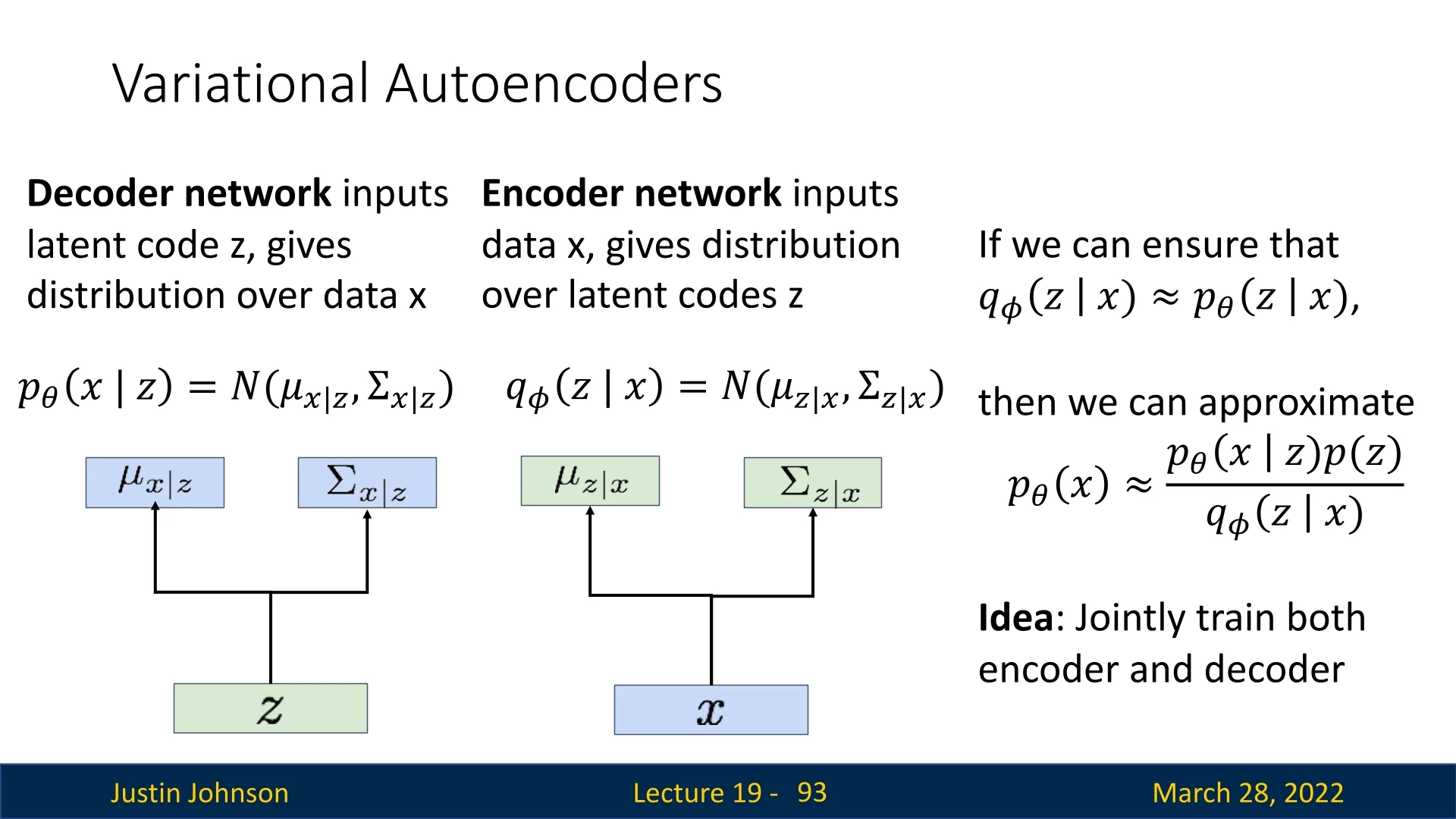
In the following sections, we will make this optimization practical (via the reparameterization trick) and then compare VAEs to alternative generative modeling approaches such as autoregressive models and GANs.