Lecture 13: Object Detection
13.1 Object Detection: Introduction
This chapter shifts our focus from image classification to object detection—the task of finding and localizing multiple objects in an image with bounding boxes. Unlike classification, which assigns a single label per image, detection must identify several objects and their positions.
In the 2022 course, object detection and segmentation are introduced earlier than in previous versions (which covered RNNs, Attention, and Transformers first). Later chapters will revisit these tasks using modern approaches like Vision Transformers, reflecting SOTA results as of early 2025.
13.1.1 Computer Vision Tasks: Beyond Classification
So far, we have primarily focused on image classification, but there exist other important tasks in computer vision:
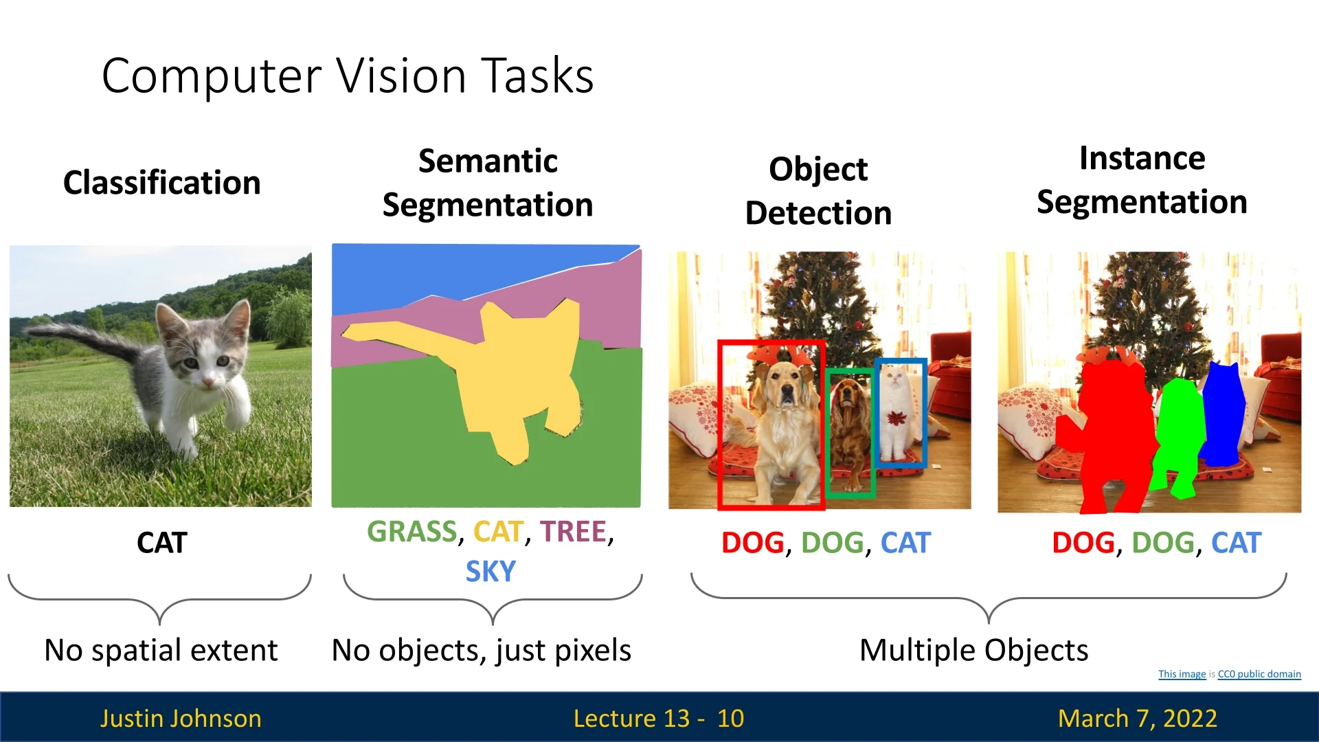
Figure 13.1 compares different object-related computer vision tasks. It starts by object classification, which we’ve covered extensively up to this point. Then proceeds with semantic segmentation, that classifies pixels without identifying individual object instances. Then, it shows object detection that assigns category labels to multiple objects while also localizing them with bounding boxes, and finishes with instance segmentation that refines detection by also delineating object boundaries.
13.1.2 What is Object Detection?
Object detection is a fundamental problem in computer vision that unifies classification (“what is it?”) and localization (“where is it?”) into a single task. Given an RGB image as input, the model outputs a set of predictions, each describing one detected object through:
- A bounding box—typically four real numbers, either \((x, y, w, h)\) for the top-left corner, width, and height, or \((c_x, c_y, w, h)\) for center coordinates.
- A category label drawn from a fixed set of known classes (e.g., the 80 categories in COCO such as “person”, “car”, “dog”).
Each prediction may also include a confidence score indicating how likely the detection is correct. Unlike image classification, which assumes a single dominant object per image, detection must handle multiple, possibly overlapping instances—each with independent localization and classification.
Closed-Set vs. Open-Set Detection Traditionally, object detection has been formulated as a closed-set problem: the detector is trained to recognize objects only from a fixed, predefined vocabulary (for example, the 20 PASCAL VOC classes or the 80 COCO classes). Classic frameworks developed throughout the 2010s—beginning with R-CNN, followed by Fast R-CNN, and later Faster R-CNN—all operate in this regime. They take a region in an image and assign it to one of the known classes (plus a “background” class), and each new version mainly improved efficiency and training integration, not the underlying assumption about the label set.
This design has an important consequence: such models can only recognize categories that were present during training. If a deployed system suddenly needs to detect a “microwave” or an “electric scooter” that was not part of the original label list, we typically must collect new annotated data and retrain or at least fine-tune the detector. In practice, this does not scale well. Real-world environments contain a very long tail of rare or domain-specific objects (industrial tools, medical devices, new product types, new traffic signs), and it is rarely feasible to anticipate and label all of them in advance. Moreover, people naturally think and communicate in language, not in class indices: a user might want to search for “all red umbrellas”, “people holding phones”, or “damaged cars”, even if such fine-grained concepts were never defined as separate classes in the training set.
These limitations motivate the move to open-set (or open-vocabulary) detection. In the open-set setting, the model is no longer restricted to predicting from a fixed list of labels. Instead, it accepts text prompts that describe what to detect, and learns to align image regions with those textual descriptions. This enables zero-shot generalization: the detector can localize objects that it has never seen as explicit labels during training, such as “a red umbrella” or “a brown horse with a rider”, by composing its learned notions of color, object type, and relationships.
This shift from closed-set to open-set detection is a conceptual breakthrough for two main reasons:
- Scalability of the vocabulary. The detectable label space is no longer hard-coded into the network; it is as rich as the language used to query it. Adding a new concept often amounts to changing the text prompt, not retraining on new bounding-box annotations.
- Natural, language-based interaction. Users can express what they are looking for in free-form text, narrowing or broadening the query as needed. This makes object detection much easier to integrate into real applications, such as interactive search in large image or video collections, without redesigning the model each time the task changes.
Representative open-set (open-vocabulary) detectors include:
- Grounding DINO [384] links image regions to free-form text descriptions by jointly training on images and captions, using a transformer-style architecture that we will encounter later in the book. This enables text-conditioned detection and phrase grounding in natural language.
- OWL-ViT [446] builds on vision transformers to align image patches and text in a shared embedding space. At test time, it can localize objects described by new text prompts (zero-shot detection), without retraining on those categories.
- OWL-ViT v2 [444] improves both efficiency and the quality of the text–region alignment, achieving stronger open-vocabulary performance on benchmarks such as COCO and LVIS.
- YOLO-World [101] adapts the fast YOLO detection family to the open-vocabulary setting, combining lightweight detection heads with text-conditioned features to support real-time, prompt-driven detection on video streams.
These models blur the boundary between object detection and visual grounding: instead of predicting from a fixed label list, they learn a shared representation for images and text and then match them at inference time. The key ingredients behind this capability—transformers, large-scale vision–language pretraining, and joint embedding spaces—will be introduced more formally in later chapters.
Scope of This Chapter In this chapter and its consequent one, we focus on the classic closed-set object detection framework: starting from region proposal methods in R-CNN, moving through Fast R-CNN and Faster R-CNN, and touching on early single-stage detectors such as YOLO. These systems form the conceptual backbone of modern detection, illustrating how detectors generate candidate regions, predict bounding boxes, refine localization, and assign class confidences. After placing these foundations, in later chapters we will briefly revisit open-set and text-driven detection to show how the same principles are extended when the fixed label vocabulary is replaced by natural-language prompts and large vision–language models.
13.1.3 Challenges in Object Detection
Compared to classification, object detection presents several unique challenges:
- Multiple objects per image: Unlike classification, where a single label is predicted, detection requires a variable number of outputs since the number of objects in an image is unknown beforehand.
- Multiple types of outputs: The model must predict both category labels (classification) and bounding box coordinates (regression).
- Large images: While classification typically works on small images (e.g., \(224 \times 224\)), object detection often requires higher resolution (\(\sim 800 \times 600\)) to detect small objects effectively.
- Objects of varying scales: A single image can contain objects of drastically different sizes, requiring multi-scale feature representations.
13.1.4 Bounding Boxes and Intersection over Union (IoU)
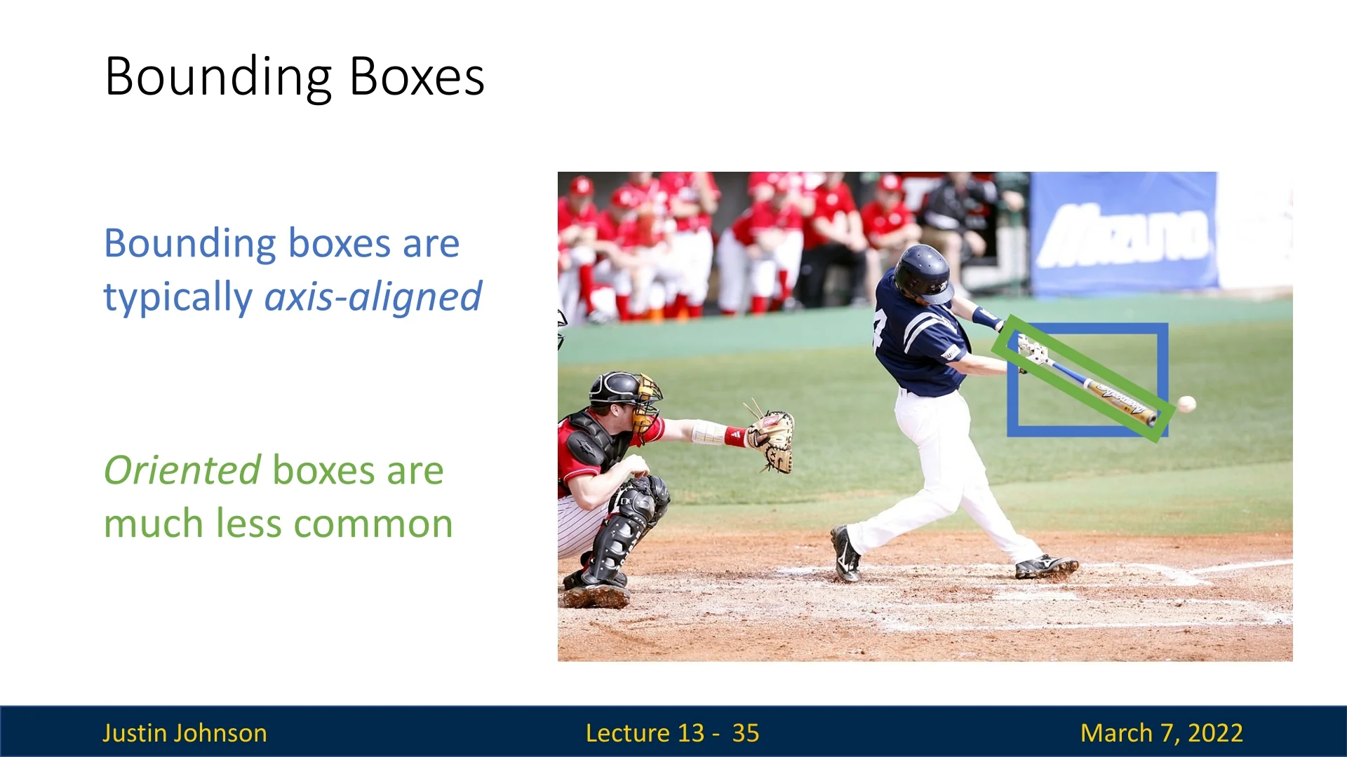
Bounding boxes are typically axis-aligned, meaning they are parallel to the image axes and not rotated. Although oriented bounding boxes (which allow rotation) can capture object shapes more precisely—especially for elongated or tilted objects—they are seldom used in general-purpose detection because they increase annotation and model complexity.
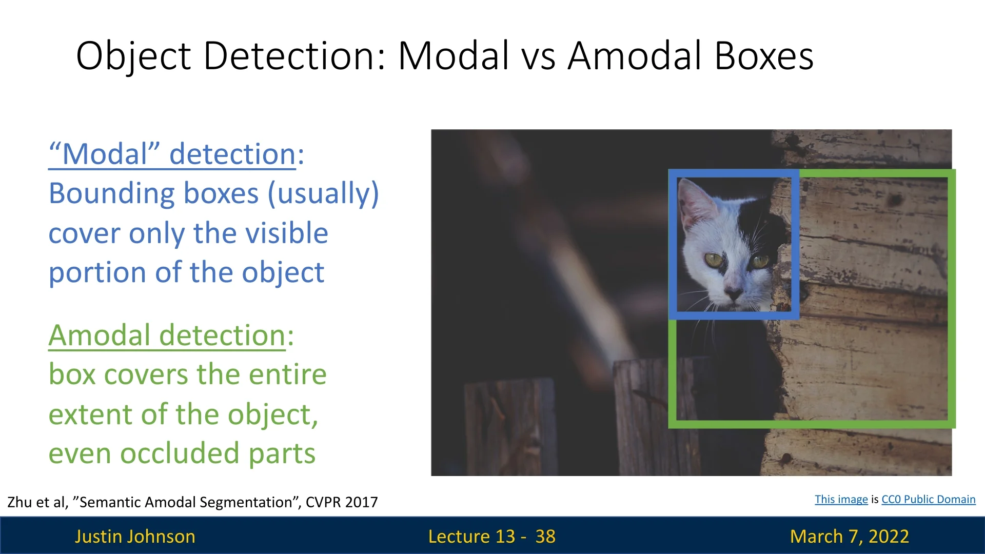
Bounding boxes can also differ in how they treat occlusion:
- Modal boxes: Enclose only the visible part of an object.
- Amodal boxes: Enclose the entire object, including occluded or truncated regions.
A crucial practical point is that the choice between modal and amodal labeling must be consistent throughout the dataset and evaluation pipeline. Metrics such as Intersection over Union (IoU) are highly sensitive to this definition: a detector trained to predict amodal boxes will systematically score lower on a benchmark annotated with modal boxes (and vice versa), even if its predictions are visually correct. Thus, maintaining clear, dataset-wide agreement on the bounding box convention is essential for meaningful training, fair comparison, and reproducible evaluation.
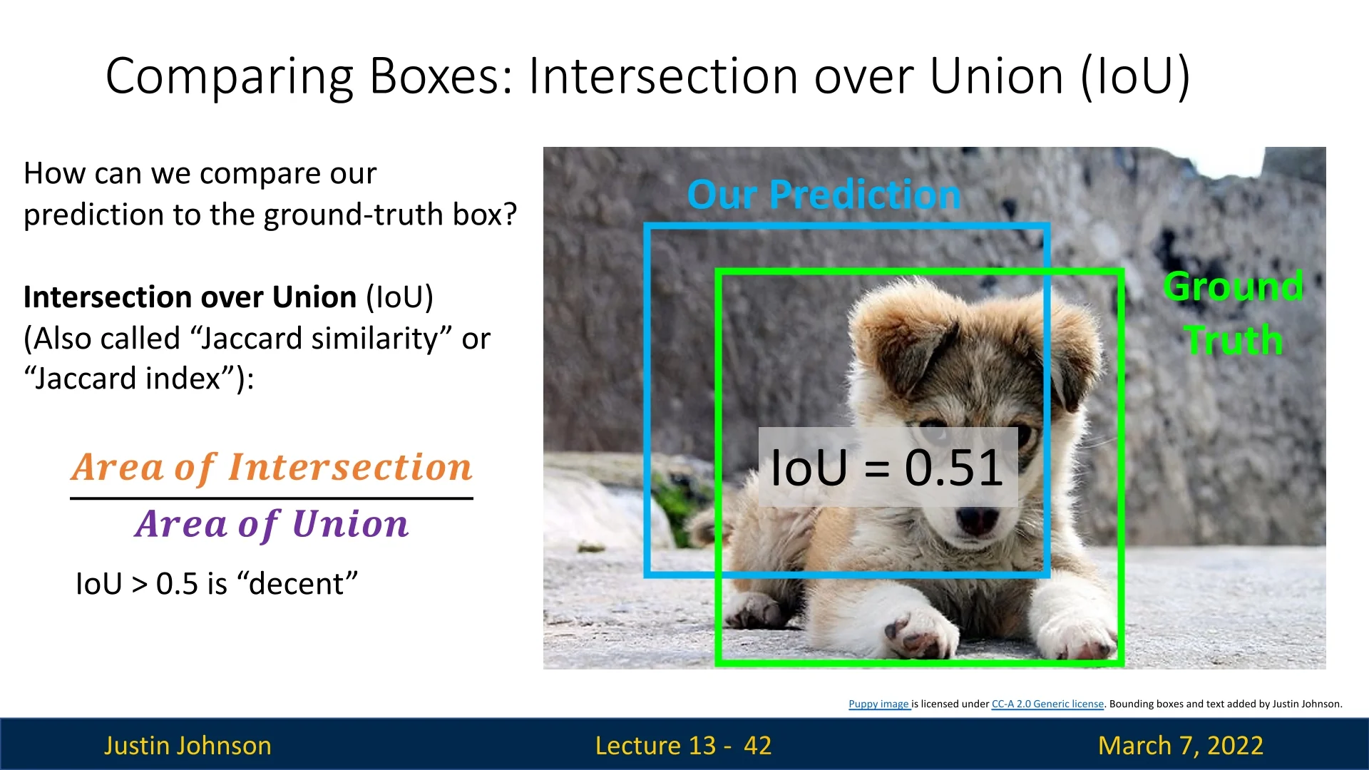
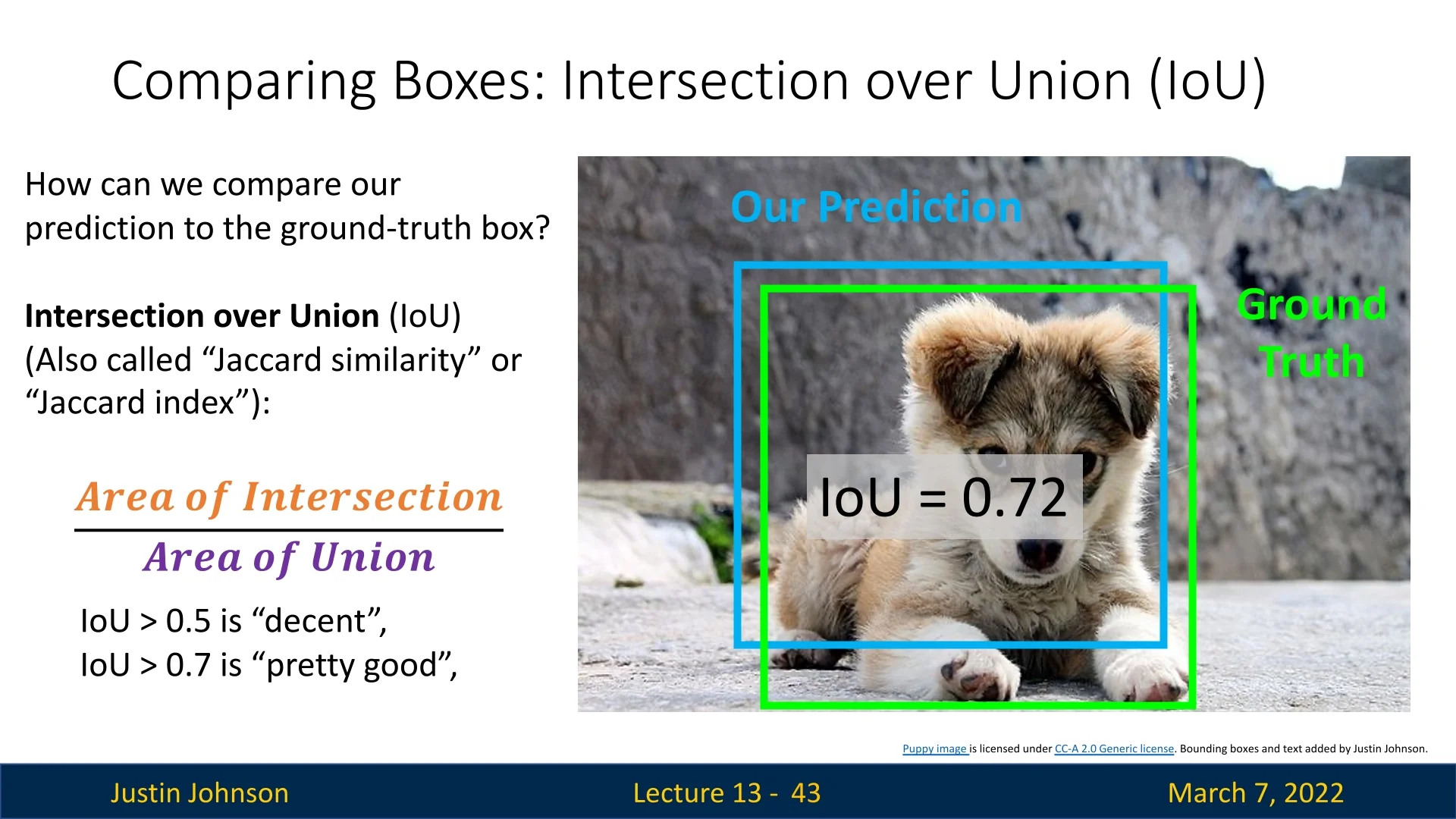
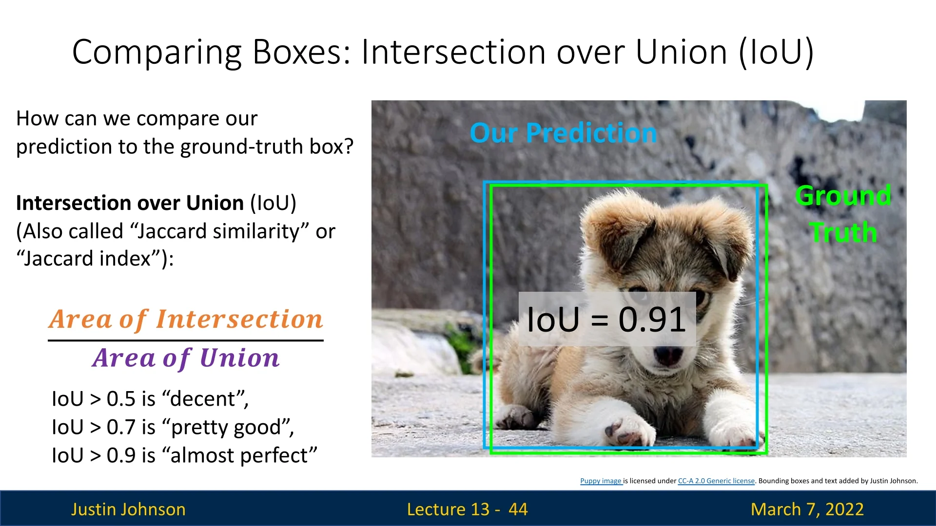
13.1.5 Evaluating Bounding Boxes: Intersection over Union (IoU)
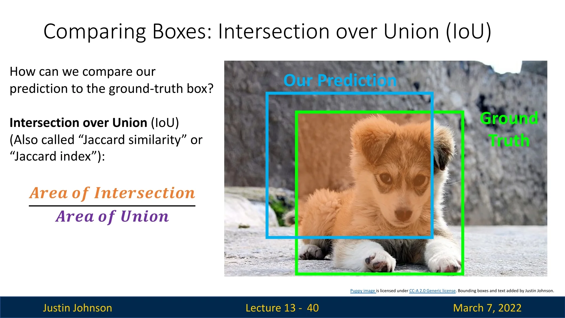
A key metric in object detection is Intersection over Union (IoU), which measures the overlap between a predicted bounding box and a ground-truth bounding box:
\[ \mbox{IoU} = \frac {\mbox{Area of Intersection}}{\mbox{Area of Union}} \]
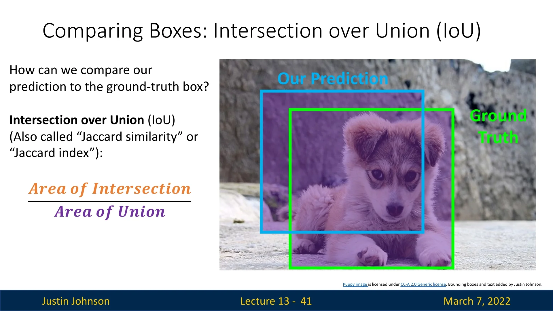
Higher IoU values indicate better localization:
- IoU ¿ 0.5: Decent detection.
- IoU ¿ 0.7: Good detection.
- IoU ¿ 0.9: Near-perfect match.
13.1.6 Multitask Loss: Classification and Regression
Object detection models must predict both class labels and bounding box coordinates, requiring a multi-task loss function. The loss is typically formulated as:
\[ \mathcal {L} = \mathcal {L}_{\mbox{cls}} + \lambda \mathcal {L}_{\mbox{reg}} \]
where:
- \(\mathcal {L}_{\mbox{cls}}\) is the classification loss (e.g., cross-entropy for category prediction).
- \(\mathcal {L}_{\mbox{reg}}\) is the regression loss (e.g., L2 loss for bounding box coordinates).
- \(\lambda \) is a weighting factor to balance classification and localization.
13.2 From Single-Object to Multi-Object Detection
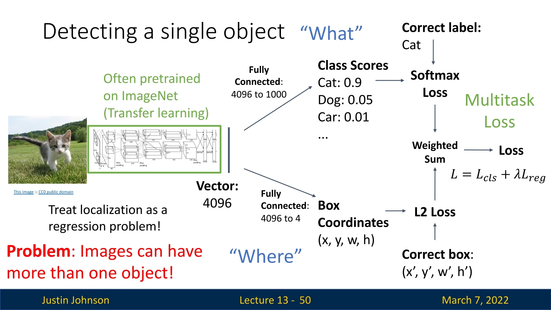
If an image contains a single object, we can extract a feature vector using a CNN (often pretrained on ImageNet) and use it for classification (category label) and regression (bounding box prediction). This works well for single-object detection but fails when multiple objects appear in an image. Hence, we need another approach in order to solve the problem in the common use-case.
13.2.1 Challenges in Detecting Multiple Objects
So far, we have focused on single-object detection. However, most real-world images contain multiple objects, making the problem significantly more challenging. This introduces key challenges:
- Variable number of outputs: The number of objects per image is unknown and must be dynamically determined.
- Multiple types of outputs: Each detected object must have both a class label and a bounding box.
- Handling overlapping predictions: The model may output multiple overlapping boxes for the same object.
To address these, early object detection models explored different solutions. In the next sections we’ll cover the progression of these solutions, starting from a naive one like sliding windows, advancing to region proposals, integrated in region-based CNNs (R-CNNs), and continue up to the more advanced solutions used in practice today.
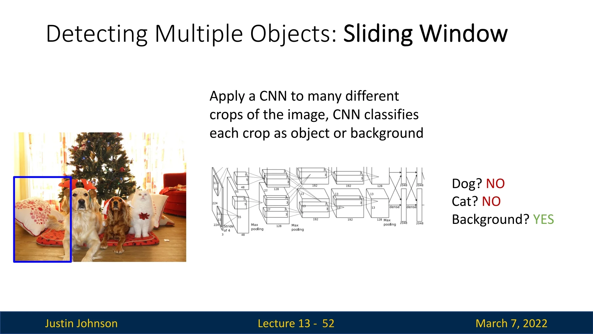
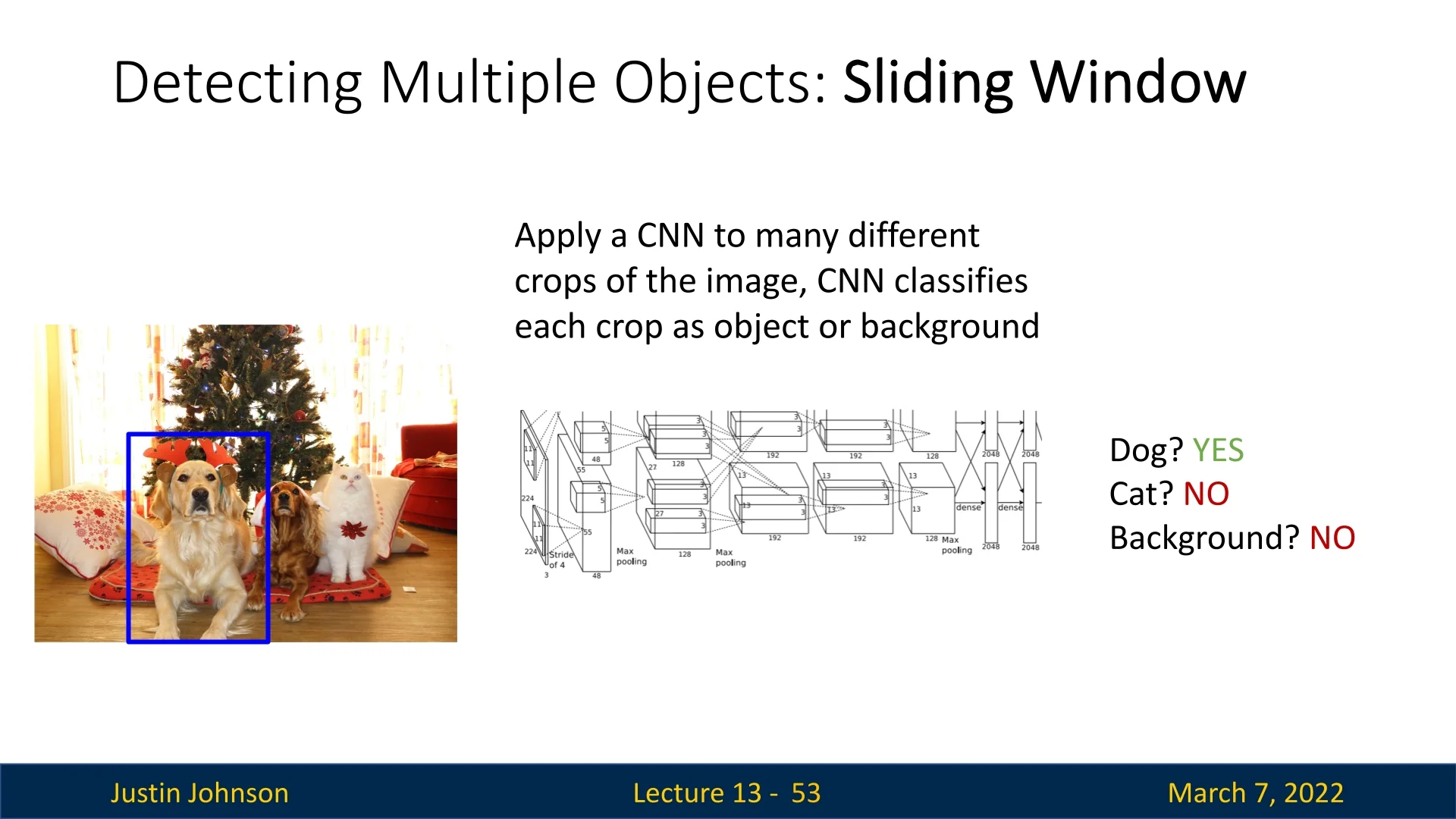
13.2.2 Sliding Window Approach
A straightforward approach is the sliding window method:
- Apply a CNN to many different crops of the image.
- Classify each crop as either an object category or background.
For example, in the below figure, we classify two different regions: one containing an object and another containing only background.
However, this approach is highly inefficient. The number of possible bounding boxes in an image of size \(H \times W\) is:
\[ \sum _{h=1}^{H} \sum _{w=1}^{W} (W - w + 1)(H - h + 1) = \frac {H(H+1)}{2} \cdot \frac {W(W+1)}{2} \]
For an \(800 \times 600\) image, this results in approximately 58 million possible boxes, making exhaustive evaluation infeasible.
13.2.3 Region Proposal Methods
To improve efficiency over sliding windows, we use region proposals, which offer several advantages:
- Efficiency: Instead of evaluating millions of possible boxes in a sliding window approach, region proposals generate a much smaller set of likely object-containing regions.
- Higher Object Coverage: These methods focus on regions that are likely to contain objects, reducing the number of unnecessary background classifications.
- Structural Awareness: Region proposals are designed to align with object boundaries better than blindly sliding fixed windows across an image.
A classical method, Selective Search, generates approximately 2000 region proposals in a few seconds on a CPU. This was a significant step forward but was still relatively slow. As deep learning advanced, heuristic-based approaches such as Selective Search were replaced by Region Proposal Networks (RPNs), which we will cover later.
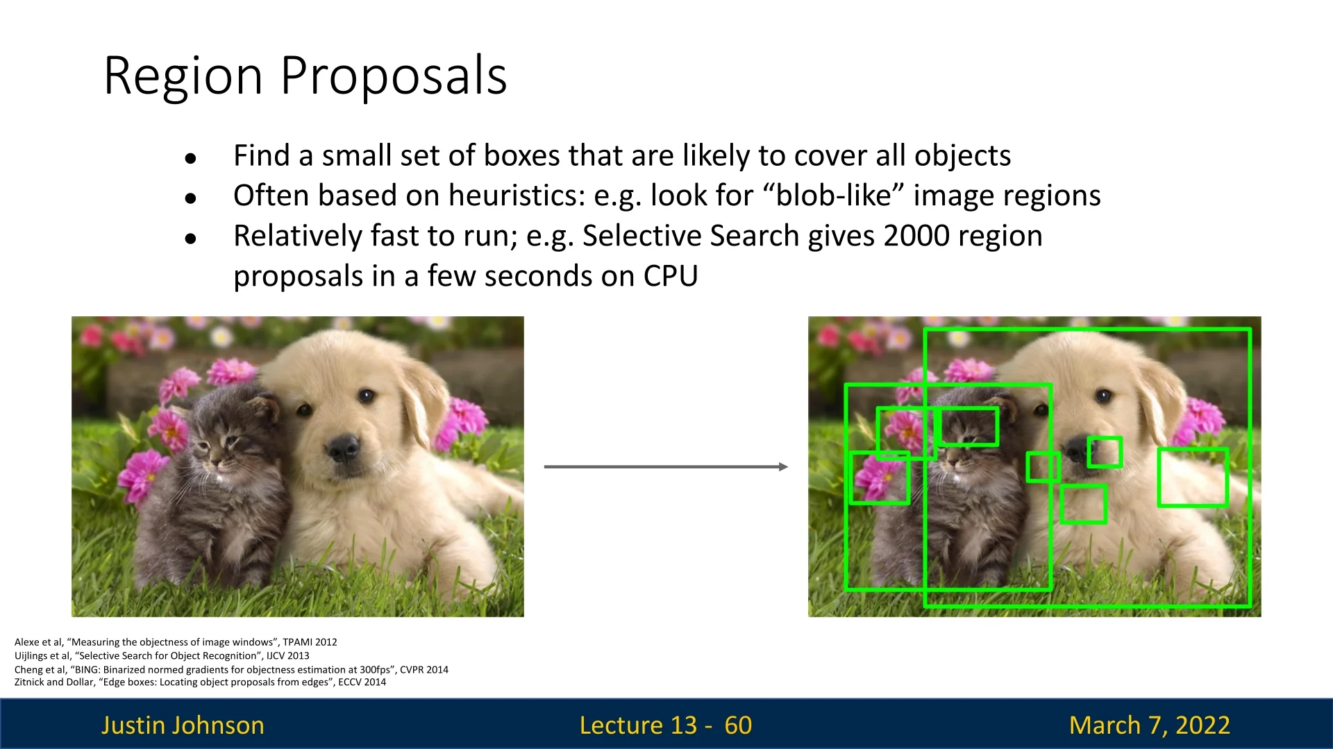
Several historical methods were used to generate region proposals:
- Alexe et al., “Measuring the objectness of image windows” (TPAMI 2012) [6]
- Uijlings et al., “Selective Search for Object Recognition” (IJCV 2013) [658]
- Cheng et al., “BING: Binarized normed gradients for objectness estimation at 300fps” (CVPR 2014) [104]
- Zitnick and Dollar, “Edge boxes: Locating object proposals from edges” (ECCV 2014) [830]
While these methods were widely used, they have since been largely replaced by faster and more accurate deep-learning-based approaches, such as Region Proposal Networks (RPNs), which we will discuss later.
13.3 Naive Solution: Region-Based CNN (R-CNN)
The first CNN-based object detection pipeline, R-CNN, was introduced by [182] in CVPR 2014. The model improved upon traditional region proposal methods by leveraging deep learning for classification and regression. The process consists of three key steps:
- 1.
- Extract region proposals: Use an external method like Selective Search to generate \(\sim \)2000 proposals per image.
- 2.
- Wrap each proposal to a fixed size: CNNs require fixed-size inputs, so each region is resized to a uniform shape (e.g., \(224 \times 224\)) to ensure consistency when passing them through the network.
- 3.
- Forward pass through a CNN: A CNN extracts features for each proposal and passes them through a classification branch to assign object labels.
- 4.
- Forward the extracted CNN features and the predicted label to a regression branch: in R-CNN, the branch takes the form of an external bounding box regressor. Each regressor was trained for a specific object label. The regressors predict transformations that refine the corresponding region proposals into accurate bounding boxes.
The reason for wrapping proposals into a fixed size is that convolutional networks are usually not ’fully’ convolutional, and hence require a consistent input resolution. Since region proposals can have varying aspect ratios and sizes, they must be resized before being processed by the CNN.
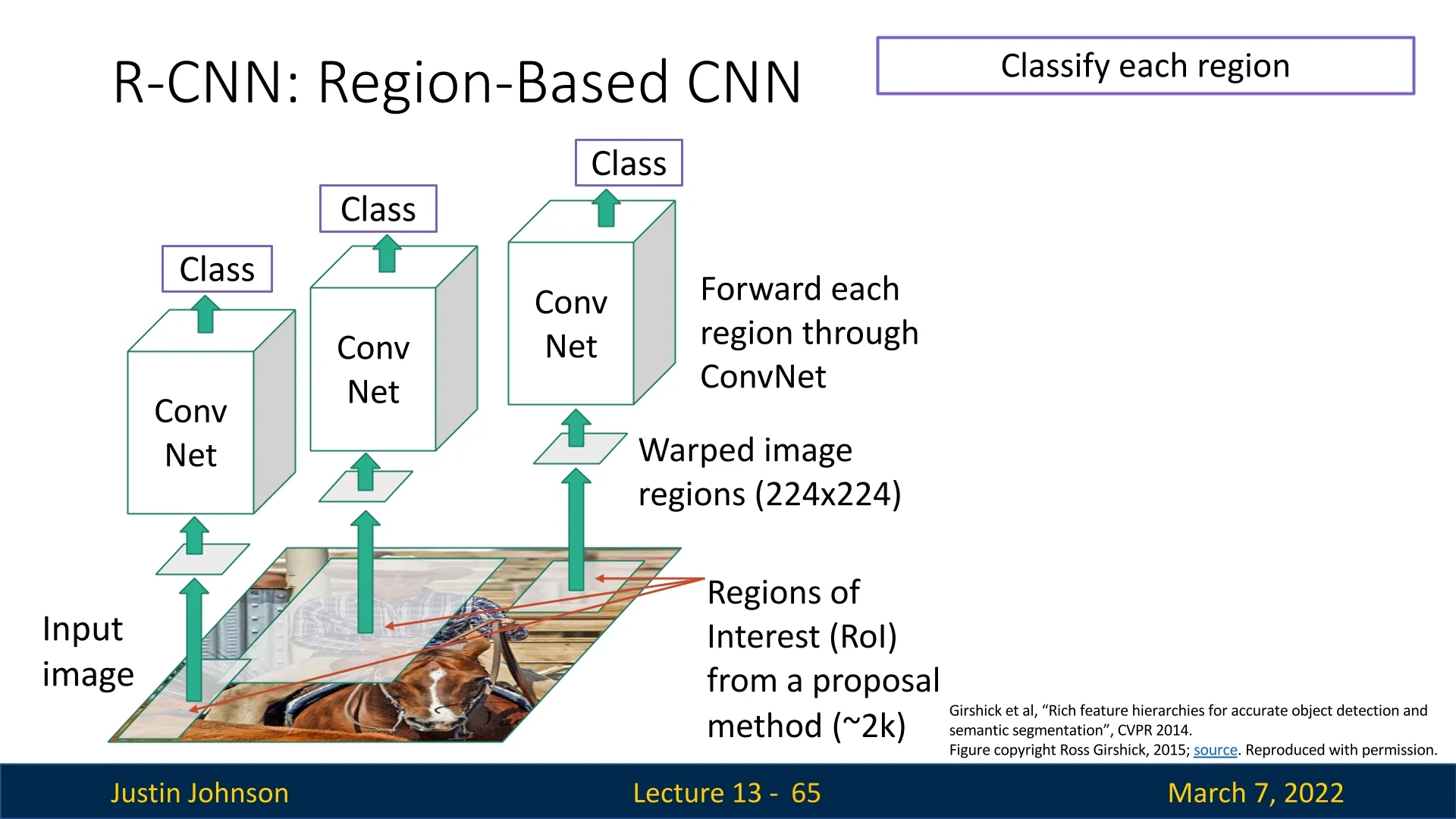
Although R-CNN improved detection speed over sliding windows by using a shared CNN for feature extraction, it remained computationally expensive because each proposal had to be passed through the CNN separately. Later models, such as Fast R-CNN, introduced optimizations to address this inefficiency, as we’ll see later.
13.3.1 Bounding Box Regression: Refining Object Localization
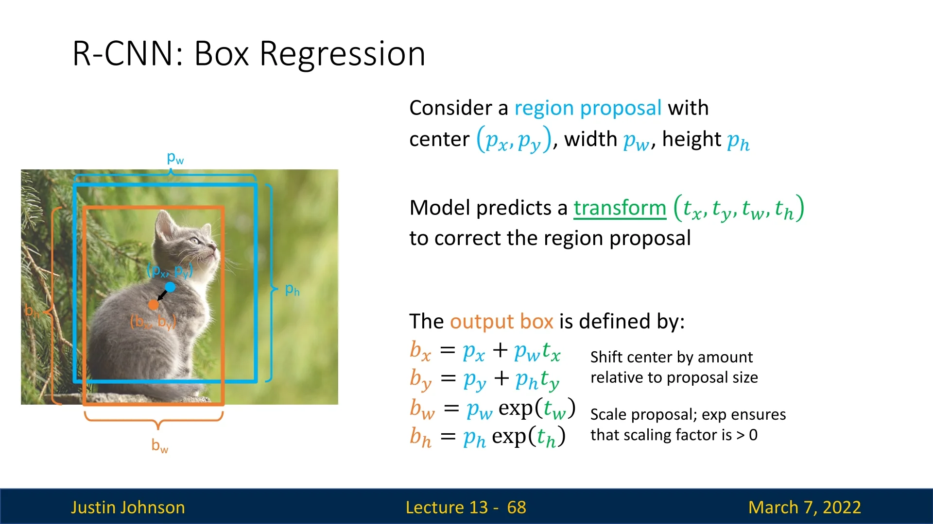
While R-CNN classifies each proposed region, the proposals themselves are generated using heuristic methods that may not precisely fit objects. To address this, R-CNN introduces bounding box regression:
- Alongside classification, an external regressor also predicts four transformation values \( (t_x, t_y, t_w, t_h) \).
- These values adjust the region proposal to better fit the object by slightly shifting and scaling the bounding box.
Refining bounding boxes is crucial because region proposals are often imprecise, covering background pixels or missing parts of the object. Without adjustments, classification accuracy may suffer, and the object localization aspect of our solution would remain inaccurate.
Bounding boxes can be represented in multiple ways. Among them, two of the most common ones are:
- Top-left notation: \((x, y, w, h)\), where \((x, y)\) is the top-left coordinate and \((w, h)\) denote width and height.
- Center notation: \((p_x, p_y, p_w, p_h)\), where \((p_x, p_y)\) is the center coordinate and \((p_w, p_h)\) denote width and height.
By tracking the center pixel movement rather than directly modifying absolute coordinates, transformations become more intuitive, as shifts are relative to the size of the proposal. This also ensures consistency across objects of different scales. Hence, the center notation is used in this case. Note that although we are using the center notation when discussing about transformations, these representations are interchangeable and can be easily converted.
With center notation, the adjusted bounding box is computed as:
\[ b_x = p_x + p_w t_x, \quad b_y = p_y + p_h t_y \]
\[ b_w = p_w e^{t_w}, \quad b_h = p_h e^{t_h} \]
Why a Logarithmic Transformation?
- Ensuring Positive Scales: Using \(\exp (t_w)\) and \(\exp (t_h)\) ensures that the width and height remain strictly positive, preventing invalid bounding boxes.
- Making Scaling Differences Linear: Object sizes vary dramatically. Predicting scale in log-space makes large differences more manageable by converting multiplicative scale factors into additive ones.
- Stabilizing Training and Gradients: Small absolute differences in large bounding boxes correspond to much smaller relative differences than in small ones. Logarithmic scaling normalizes these variations, leading to more stable gradients and easier optimization.
Given a proposal and a GT bounding box, we can solve for the transform the network should output. The model can thus be trained to minimize the difference between predicted and ground-truth boxes using regression targets:
\[ t_x = \frac {b_x - p_x}{p_w}, \quad t_y = \frac {b_y - p_y}{p_h}, \quad t_w = \log \frac {b_w}{p_w}, \quad t_h = \log \frac {b_h}{p_h} \]
Bounding box regression significantly improves object detection performance by ensuring that detected objects are properly localized. This technique is a key component of modern object detection frameworks.
13.3.2 Training R-CNN
1) Collecting Positive and Negative Examples
- Generating Region Proposals: For each training image, we run a region proposal algorithm (e.g., Selective Search) to generate roughly 2k proposals of various sizes and aspect ratios.
-
Labeling: As illustrated in the blow figure, we compare each proposal to every ground-truth bounding box.
- Positive if \(\mbox{IoU} \ge 0.5\) with some ground-truth box of a particular class.
- Negative if \(\mbox{IoU} < 0.3\) with all ground-truth boxes (i.e., sufficiently far from every GT box).
-
Neutral if \(0.3 \le \mbox{IoU} < 0.5\). Such proposals are neither clearly positive nor clearly negative, so we typically omit them from training.
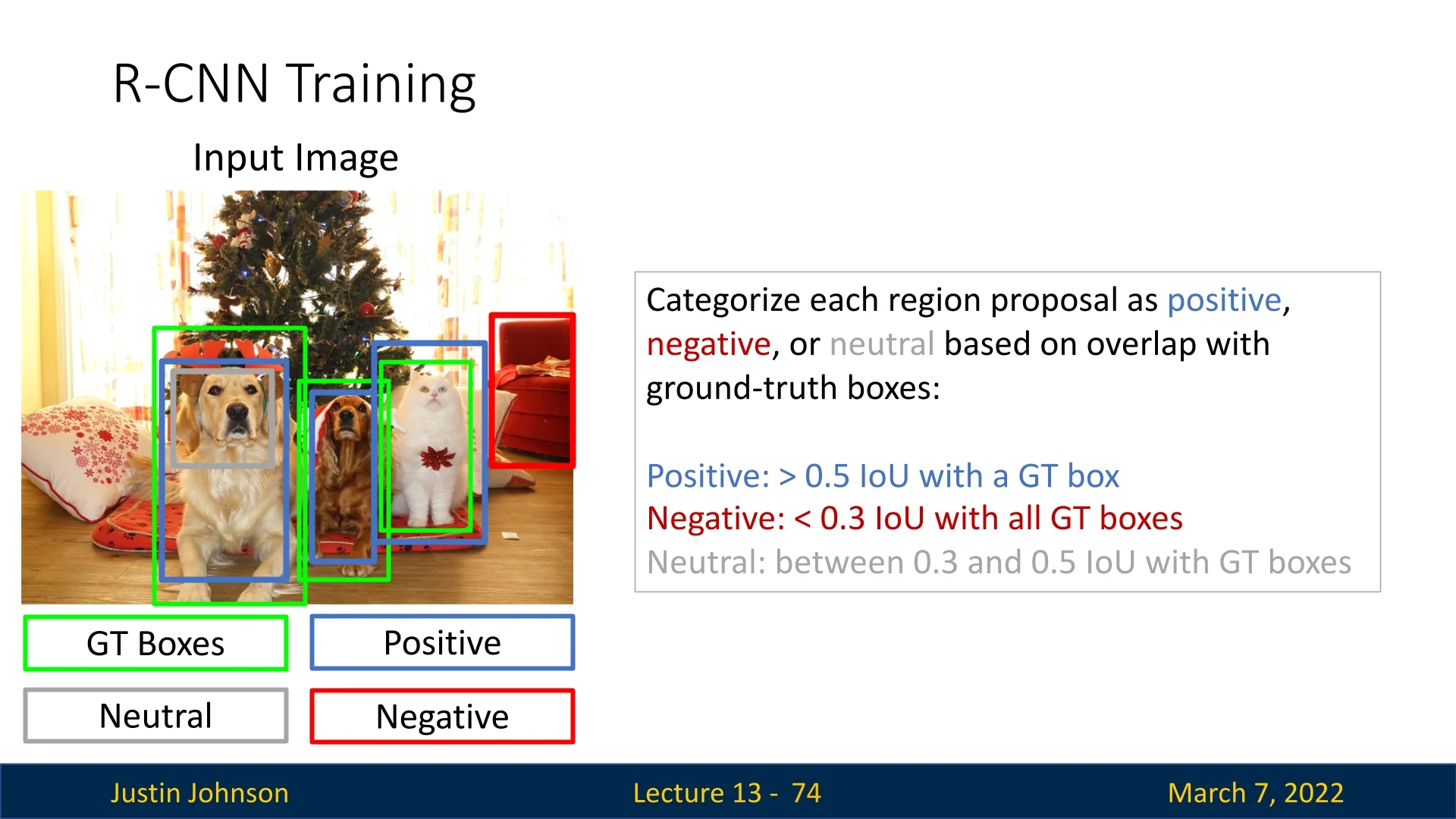
Figure 13.12: Positive vs. Negative vs. Neutral Region Proposals. An example image (green bounding boxes are ground-truth). Each region proposal is categorized as: Positive (blue) if its IoU with a ground-truth box is above 0.5, Negative (red) if its IoU is below 0.3, Neutral (gray) otherwise. Neutral proposals are typically ignored when training SVMs or fine-tuning, thus avoiding ambiguous overlap ranges.
2) Fine-Tuning the CNN on Region Proposals (Classification Only) During this stage, the CNN is adjusted to classify each region proposal into one of \(C + 1\) categories: \(C\) foreground classes plus a “background” class.
-
Training Objective:
- We replace the final fully-connected layer from the pre-trained CNN (which had been trained for ImageNet classification) with a new \((C + 1)\)-way softmax layer.
- Important: This stage only learns a classifier. We are not yet learning bounding box regression parameters here.
-
Batch Composition:
- Typically, each mini-batch is a mix of positive and negative examples.
- A common rule of thumb is to use a 1:3 or 1:4 ratio of positives to negatives. Since negatives are far more numerous, this ratio prevents them from overwhelming the training.
- Each mini-batch might pull examples from multiple training images to diversify the proposals within each batch.
-
Fine-Tuning Protocol:
- We usually start SGD at a small learning rate (e.g., \(\eta = 0.001\)), to avoid disrupting the pre-trained weights too drastically.
- In each SGD iteration, we pick a mini-batch of (say) 128 region proposals, typically containing 32 positives and 96 negatives.
- Training iterates for tens of thousands of mini-batches, often taking several hours or days depending on GPU resources and network size.
Step 3: Training the Bounding Box Regressors After fine-tuning the CNN for classification (Step 2), the final stage addresses a critical shortcoming: region proposals from Selective Search are intentionally generous—they often capture too much background or miss object boundaries. R-CNN remedies this with a lightweight yet powerful component: a bounding box regressor that learns to refine coarse proposals, nudging them closer to the true object extents.
-
Feature Source and Architecture: The R-CNN framework employs the AlexNet architecture [318], composed of five convolutional layers (conv1–conv5) followed by two fully connected layers (fc6 and fc7). The convolutional stack extracts spatially organized features such as edges and parts, while the fully connected layers distill these into high-level semantic embeddings. For each region of interest (ROI), the proposal is cropped, warped to a fixed resolution (typically \(227 \times 227\)), and fed through the network. The resulting activations from either:
- pool5 — the last pooling layer, preserving coarse spatial layout and shape.
- fc6 — a 4096-dimensional semantic representation capturing appearance and texture.
serve as the region’s feature descriptor. These same features were used by the per-class SVMs in Step 2, ensuring the regressor operates within the same feature space as classification—bridging semantic understanding and geometric adjustment.
-
Per-Class Linear Regression: For each of the \(C\) foreground classes, a separate linear model is trained to map the region’s feature vector to four transformation parameters \((t_x, t_y, t_w, t_h)\) that describe how to move and resize a proposal box \(P = (p_x, p_y, p_w, p_h)\) (center and size) toward its matching ground-truth box \(B = (b_x, b_y, b_w, b_h)\): \[ t_x = \frac {b_x - p_x}{p_w}, \quad t_y = \frac {b_y - p_y}{p_h}, \quad t_w = \ln \!\left (\frac {b_w}{p_w}\right ), \quad t_h = \ln \!\left (\frac {b_h}{p_h}\right ). \] This formulation is deliberately chosen for stability and generalization:
- Translation offsets \((t_x, t_y)\) are normalized by the proposal’s width and height, making the regression scale-invariant.
- Width and height ratios \((t_w, t_h)\) are predicted in log-space, turning multiplicative scaling (e.g., doubling width) into additive learning, which linear models handle more effectively.
In essence, the regressor learns how much to shift and stretch a box, not where to place it from scratch.
-
Training Objective: Each regressor is trained only on positive proposals—those with Intersection-over-Union (IoU) \(\ge 0.5\) with a ground-truth object. For every positive ROI:
- 1.
- Extract its feature vector (pool5 or fc6) as input.
- 2.
- Compute its ground-truth transform \((t_x, t_y, t_w, t_h)\) as the regression target.
The model minimizes an L2 loss between predicted and true transforms: \[ \mathcal {L}_\mbox{reg} = \| \hat {t} - t \|_2^2. \] Because the model is linear and the feature dimensionality is fixed (e.g., 4096 for fc6), training is efficient—often converging within minutes once features are cached. Later methods, such as Fast R-CNN, replaced this standalone regression with a smooth L1 loss integrated directly into a multi-task training objective.
- Inference: During testing, once a proposal is classified as class \(c\), the corresponding regressor outputs \(\hat {t} = (\hat {t}_x, \hat {t}_y, \hat {t}_w, \hat {t}_h)\), which are applied to the original box to compute the refined coordinates: \[ b_x = p_x + p_w \hat {t}_x, \quad b_y = p_y + p_h \hat {t}_y, \quad b_w = p_w e^{\hat {t}_w}, \quad b_h = p_h e^{\hat {t}_h}. \] The resulting bounding box \(B = (b_x, b_y, b_w, b_h)\) is a tighter, more accurate fit around the object, effectively correcting over- or under-extended proposals.
This simple yet elegant regression module—built atop AlexNet’s semantic feature layers—plays a key role in R-CNN’s success. By coupling visual appearance with geometric adjustment, it bridges classification and localization, improving mean Average Precision (mAP) by roughly 3–4 points on PASCAL VOC. The concept of decoupling classification from regression would later inspire multi-branch designs such as Fast R-CNN and Faster R-CNN, where both tasks are trained jointly within a single network.
4) Forming the Final Detector At test time:
- 1.
- Generate region proposals (e.g., Selective Search) and warp each proposal into a fixed-size CNN input.
- 2.
- Forward pass each proposal through the CNN.
- 3.
- Apply classifier SVMs or softmax on the resulting feature vector.
- 4.
- Bounding box regression is then applied to each proposal that is classified as a particular object class.
- 5.
- Non-maximum suppression (NMS) is performed per class to obtain the final object detections. We’ll explore this part in detail later.
Training Considerations for Object Detection
Hereby several factors that influence training efficacy:
- Batch Composition. Mini-batches are typically drawn from multiple images to prevent overfitting to any single image’s proposals and to ensure diverse object representations in each batch. A standard practice is to maintain a ratio of approximately 1:3 or 1:4 between positive and negative samples. Since negative proposals (background) far outnumber positive ones (actual objects), controlling this ratio ensures balanced learning, preventing the classifier from being biased toward background predictions. Additionally, ensuring that each mini-batch contains a variety of object categories helps stabilize the learning process by allowing the model to generalize across different object types.
-
Class-Specific Bounding Box Regressors. Rather than employing a single regressor for all classes, the method trains a separate bounding box regressor for each object class. This decision is motivated by several factors:
- Distinct Geometric Characteristics: Different object classes exhibit unique aspect ratios, sizes, and shapes. For instance, the ideal bounding box adjustments for a car differ from those for a person or a bicycle. By dedicating a regressor to each class, the model can learn tailored transformation parameters that more accurately capture the variations within that class.
- Simplified Regression Task: A single regressor would need to account for the wide variability in bounding box distributions across all classes, increasing the complexity of the learning task. Class-specific regressors, on the other hand, can focus on a more homogeneous set of targets, making the regression problem easier to optimize.
- Improved Localization Accuracy: Specialization allows each regressor to adapt to the statistical properties of its corresponding class, typically resulting in more precise adjustments of the region proposals and, consequently, higher overall detection performance.
These reasons, supported by empirical evidence in the R-CNN , demonstrate that the use of class-specific regressors leads to better object localization than a unified regression model would achieve.
-
Regularization and Overfitting. Due to the high degree of overlap between region proposals, models trained without proper regularization may overfit to the specific patterns of region proposals in the training set. Strategies to mitigate this include:
- Data Augmentation: Techniques such as random cropping, rotation, and color jittering introduce variability in region proposals, making the model more robust to unseen samples.
- Dropout and Weight Decay: Regularization techniques such as dropout prevent co-adaptation of neurons, while weight decay discourages overly complex solutions that may not generalize well.
- Careful Learning Rate Scheduling: A gradual decrease in learning rate stabilizes training and prevents drastic parameter updates that could lead to overfitting.
13.3.3 Selecting Final Predictions for Object Detection
Once the model has generated transformed region proposals, we must determine which subset of them to output as final detections. Several filtering strategies exist, each with trade-offs:
- Fixed Output Count: We output a fixed number of proposals (e.g., 100), selecting those with the highest confidence scores. If fewer objects exist, many proposals may be background, but this guarantees an upper bound on computational cost.
- Per-Class Thresholding: A predefined confidence threshold is set for each category. Detections exceeding this threshold are retained, while lower-confidence predictions are discarded. This ensures that only highly confident detections are considered.
- Top-K Selection: The model retains only the top-K proposals across all categories based on classification scores. This guarantees a fixed number of high-confidence detections but may introduce false positives if \(K\) is too large.
While these methods provide an initial filtering mechanism, they often produce multiple overlapping detections for the same object. To refine the final outputs, an additional step is required to eliminate redundant bounding boxes while preserving the most confident predictions.
This naturally leads us to Non-Maximum Suppression (NMS), a widely used technique that selects the best bounding boxes while removing duplicates, ensuring a clean and interpretable final detection output.
13.4 Non-Maximum Suppression (NMS)
13.4.1 Motivation: The Need for NMS
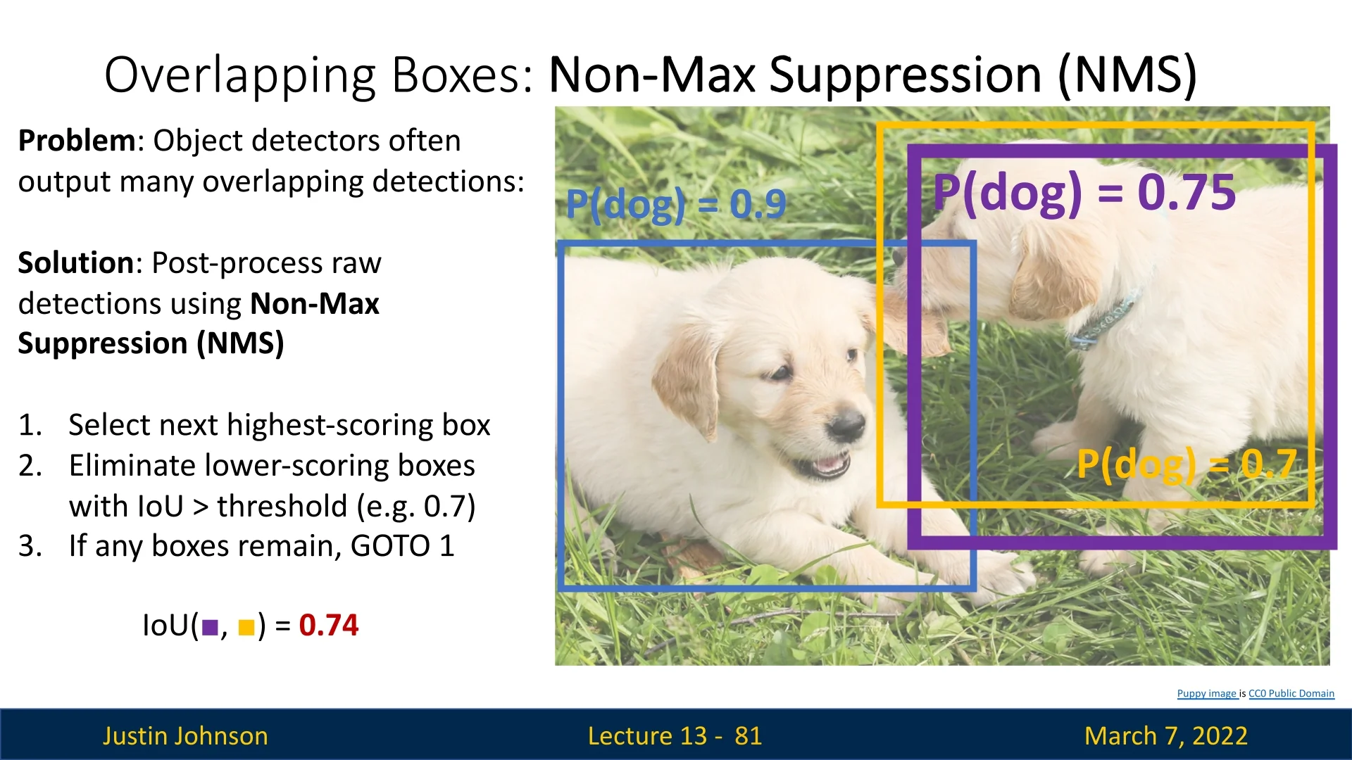
Object detectors can generate multiple, overlapping bounding boxes for a single object. This redundancy arises because:
- CNN classifiers score each region proposal independently, so similar proposals can all receive high confidence.
- Small variations in the proposals, even when they target the same object, yield multiple detections.
- Imperfections in bounding box regression can lead to slightly misaligned overlapping boxes.
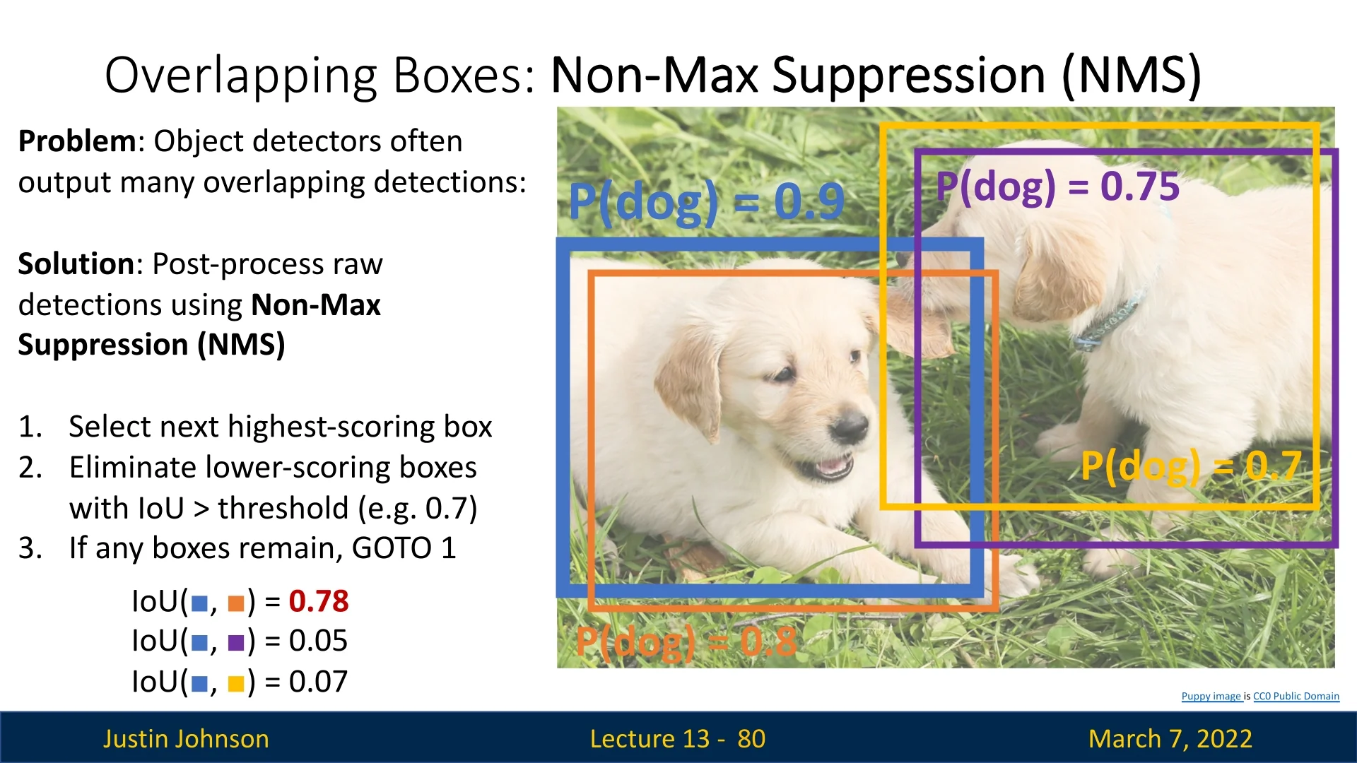
To resolve this, Non-Maximum Suppression (NMS) is applied as a post-processing step. NMS systematically removes redundant detections by retaining only the highest-scoring box among overlapping candidates, thereby improving localization accuracy and overall detection quality.
13.4.2 NMS Algorithm
Given a set of detected bounding boxes, each with a classification score, we perform NMS as follows:
- 1.
- Select the highest-scoring bounding box.
- 2.
- Compare it to all remaining boxes:
- Remove boxes with high IoU (e.g., \(\mbox{IoU} > 0.7\)) relative to the selected box.
- 3.
- Repeat until no boxes remain.
13.4.3 Example: Step-by-Step Execution
Consider the following bounding boxes predicted for a detected dog:
Now we proceed to the next highest-scoring bounding box:
No other boxes remain to be checked, so the process is finished, and we remain with the set of resultant bounding boxes to output.
13.4.4 Limitations of NMS
While Non-Maximum Suppression (NMS) is indispensable in traditional object detectors, it is ultimately a handcrafted, greedy heuristic. Its rule is simple: keep the highest-scoring box for a given object and suppress all others that overlap too much (high IoU). This approach works well when objects are well separated, but it begins to fail in crowded scenes.
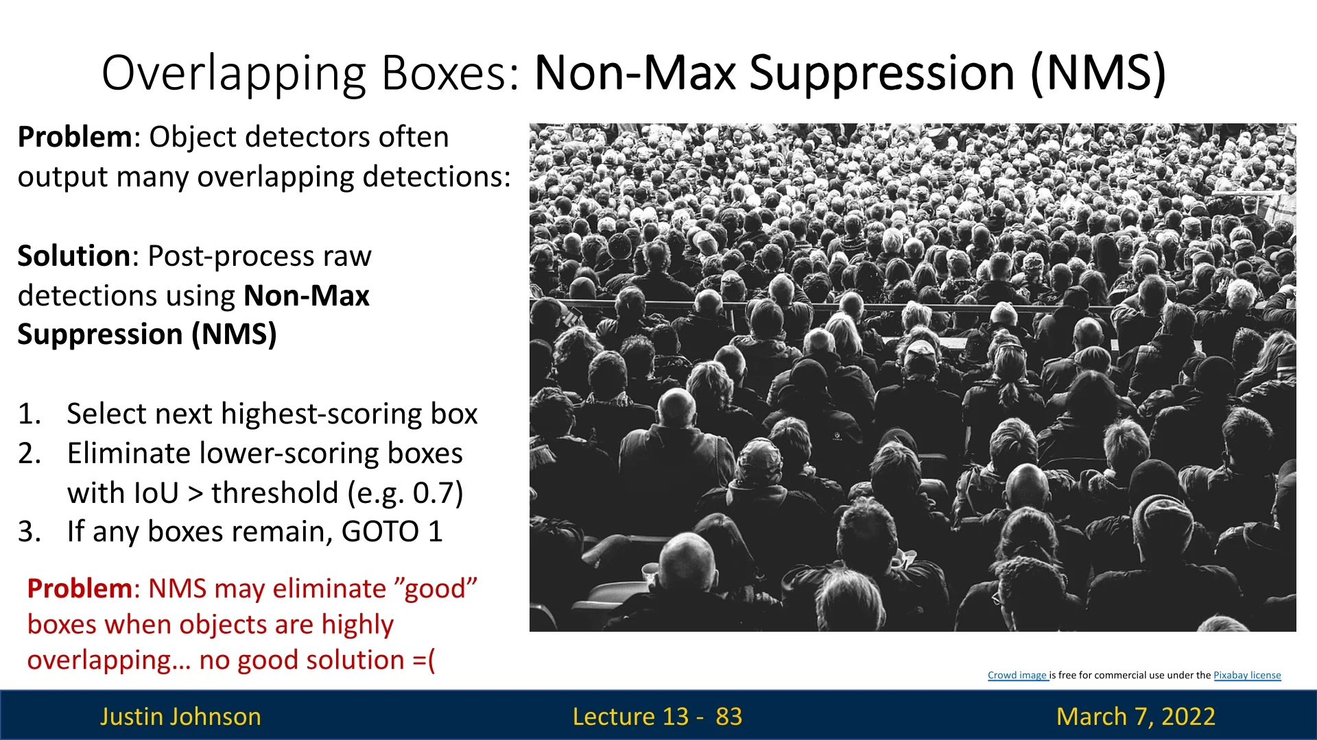
Because NMS cannot distinguish between a duplicate detection of the same object and two different objects that happen to overlap, it can wrongly remove valid boxes—for example, people standing shoulder-to-shoulder or cars in a traffic jam. Moreover, since NMS operates outside the learning process, it is not optimized jointly with the rest of the model.
These limitations have motivated a new research direction: NMS-free detection. The key idea is to design detectors that naturally produce non-redundant outputs without relying on post-processing. Instead of generating thousands of overlapping predictions, modern architectures such as DETR (DEtection TRansformer, [64]) reformulate detection as a set prediction problem. The model predicts a fixed-size set of object candidates (e.g., 100 slots), and during training, a special matching loss pairs each prediction to its corresponding ground-truth object.
This matching process is based on the Hungarian algorithm, a classic method for optimally assigning elements between two sets. Although the mathematical details are beyond the scope of this chapter, the intuition is simple: each prediction must match exactly one ground-truth object, and unmatched predictions are treated as background. By learning this one-to-one correspondence, the network inherently avoids duplicate detections—making NMS unnecessary at inference time.
These end-to-end, NMS-free detectors mark a significant conceptual shift: instead of cleaning up redundant predictions after the fact, they learn to not produce them in the first place. While such methods still face challenges (e.g., training complexity and slower convergence), they represent an important step toward fully differentiable, self-consistent detection pipelines.
13.4.5 Refining NMS for Overlapping Objects
Researchers have proposed several improvements to mitigate NMS failures:
- Soft-NMS: Instead of outright removing overlapping boxes, Soft-NMS reduces their confidence scores gradually.
- Learned NMS: Some models learn a post-processing step that dynamically adjusts suppression criteria based on object density.
- Adaptive Thresholding: Instead of using a fixed IoU threshold, we adjust it based on object size and category.
Despite these refinements, NMS and its variants remain standard in many anchor-based and dense prediction detectors because of their simplicity and efficiency, even though newer set-based, query-driven architectures such as DETR- and Grounding DINO-style models avoid NMS entirely by formulating detection as bipartite matching.
13.5 Evaluating Object Detectors: Mean Average Precision (mAP)
Evaluating object detection models is more complex than evaluating standard classification systems. In detection, we must assess both the classification of each detected object and the localization (i.e., how accurately its bounding box is predicted). Therefore, an effective evaluation metric must consider both aspects.
13.5.1 Key Evaluation Metrics
Precision and Recall Precision and recall form the foundation of object detection evaluation, quantifying how well a model balances false alarms against missed detections:
- Precision measures the proportion of correct detections among all predicted boxes: \[ \mbox{Precision} = \frac {\mbox{True Positives (TP)}}{\mbox{True Positives (TP)} + \mbox{False Positives (FP)}}. \] High precision means that most predicted boxes correspond to real objects—important in applications where false alarms are costly (e.g., automated surveillance).
- Recall measures the fraction of ground-truth objects that were successfully detected: \[ \mbox{Recall} = \frac {\mbox{True Positives (TP)}}{\mbox{True Positives (TP)} + \mbox{False Negatives (FN)}}. \] High recall indicates few missed detections—critical for safety-sensitive tasks such as pedestrian detection or medical diagnosis.
Balancing Precision and Recall Precision and recall often pull in opposite directions. Raising the detection confidence threshold improves precision (fewer false positives) but lowers recall (more misses). Different applications value different trade-offs:
- Autonomous vehicles / medical imaging: prioritize recall—better to raise false alarms than miss a pedestrian or lesion.
- Retail analytics / automated security: emphasize precision—false positives waste time or cause alert fatigue.
A single confidence threshold can reveal only one operating point on this continuum; a more complete picture requires evaluating performance across thresholds and incorporating localization accuracy.
Why the F1 Score Falls Short The F1 score, defined as the harmonic mean of precision and recall, \[ \mbox{F1} = 2 \cdot \frac {\mbox{Precision} \times \mbox{Recall}}{\mbox{Precision} + \mbox{Recall}}, \] is a useful summary in classification—but limited for object detection:
- Threshold Dependence and Limited Insight: F1 is computed at a single confidence threshold (e.g., 0.5). This snapshot hides how precision and recall trade off as we vary the threshold. In practice, a detector may perform well at high-confidence (precise but selective) or low-confidence (broad but noisy) regimes, and F1 cannot reveal these trends.
- Ignores Localization Quality: F1 counts a detection as “correct” once it passes an IoU threshold (e.g., IoU \(\ge \) 0.5) but does not reward better alignment. A slightly overlapping box and a perfectly aligned one both count equally, masking localization differences.
Hence, while F1 summarizes a single point on the precision-recall curve, it cannot characterize the full behavior of a detector or compare models robustly across varying confidence thresholds and spatial accuracies.
Precision–Recall (PR) Curve and Average Precision (AP) To capture this broader behavior, detection benchmarks use the Precision–Recall (PR) curve. It plots precision versus recall as the detection confidence threshold sweeps from high to low. The construction is as follows:
- 1.
- Sort all predicted boxes by their confidence scores in descending order.
- 2.
- Iterate over the detections: for each prediction, determine whether it
correctly matches a ground-truth box of the same class using an IoU
threshold (e.g., IoU \(\ge \) 0.5):
- If matched, mark as a True Positive (TP).
- If unmatched, mark as a False Positive (FP).
- Each ground-truth box may be matched to only one detection.
- 3.
- Compute precision and recall after each detection is added, producing a series of (Precision, Recall) pairs.
- 4.
- Plot these pairs to obtain the PR curve, which visualizes the trade-off between precision and recall as confidence decreases.
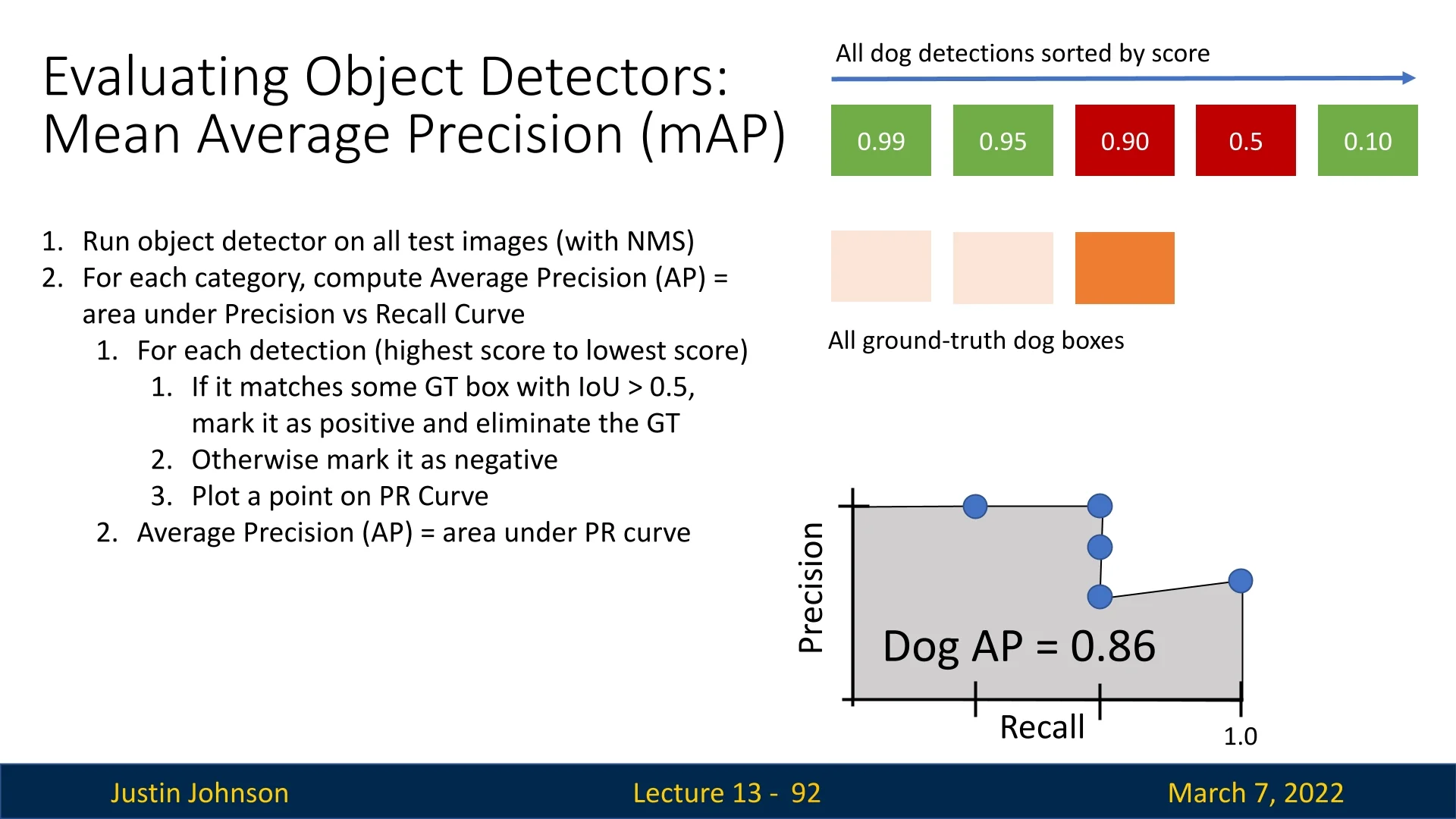
Average Precision (AP) and IoU Thresholds The Average Precision (AP) summarizes the PR curve as a single number—the area under the curve (AUC): \[ \mbox{AP} = \int _0^1 \mbox{Precision}(\mbox{Recall}) \, d(\mbox{Recall}), \] often approximated numerically (e.g., using the 11-point or all-points interpolation method). A higher AP means the model maintains good precision across a broad range of recall levels.
The subscript in AP@0.5 indicates the IoU threshold used to decide a correct match. IoU = 0.5 is the conventional standard, balancing tolerance and rigor: detections must overlap by at least 50% to count as correct. Stricter thresholds (e.g., AP@0.75) emphasize precise localization, while looser ones favor recall. Modern benchmarks like COCO report mean Average Precision (mAP) averaged over multiple IoUs (AP@[0.5:0.95]) to reflect both coarse and fine localization quality.
Why AP is Preferable to F1 AP overcomes the key shortcomings of F1:
- Comprehensive Threshold Evaluation: integrates performance over all confidence thresholds, not a single fixed point.
- Trade-off Awareness: captures the model’s entire precision–recall curve, revealing how it behaves under different operating conditions.
- Localization Sensitivity: uses IoU to determine correctness, linking classification confidence with spatial accuracy.
A perfect detector would achieve AP = 1.0—indicating flawless precision and recall at every threshold. In practice, maximizing AP (and mAP across IoUs) provides a balanced, interpretable, and widely adopted measure of object detection performance, far more revealing than single-threshold scores such as F1.
13.5.2 Step-by-Step Example: Computing AP for a Single Class
Consider the dog category with three ground-truth boxes. The process is illustrated step-by-step:
- 1.
- First detection (score: 0.99): Matches the second ground-truth box
(IoU \( > 0.5 \)).
- Precision = \( 1/1 = 1.0 \)
- Recall = \( 1/3 \approx 0.33 \)
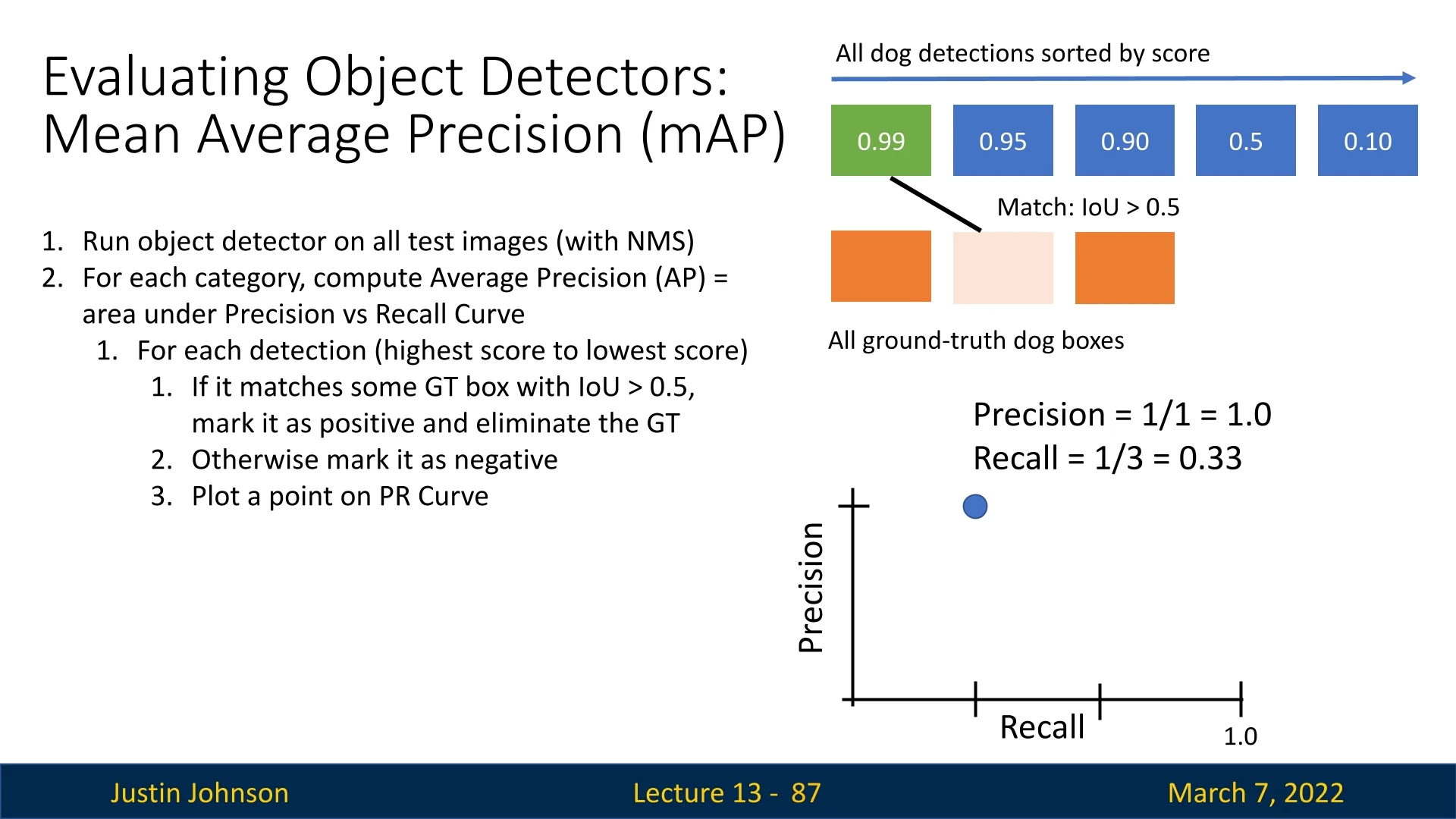
Figure 13.16: Step 1: First match. The highest-scoring detection correctly matches a ground-truth box. - 2.
- Second detection (score: 0.95): Matches the first ground-truth
box.
- Precision = \( 2/2 = 1.0 \)
- Recall = \( 2/3 \approx 0.67 \)
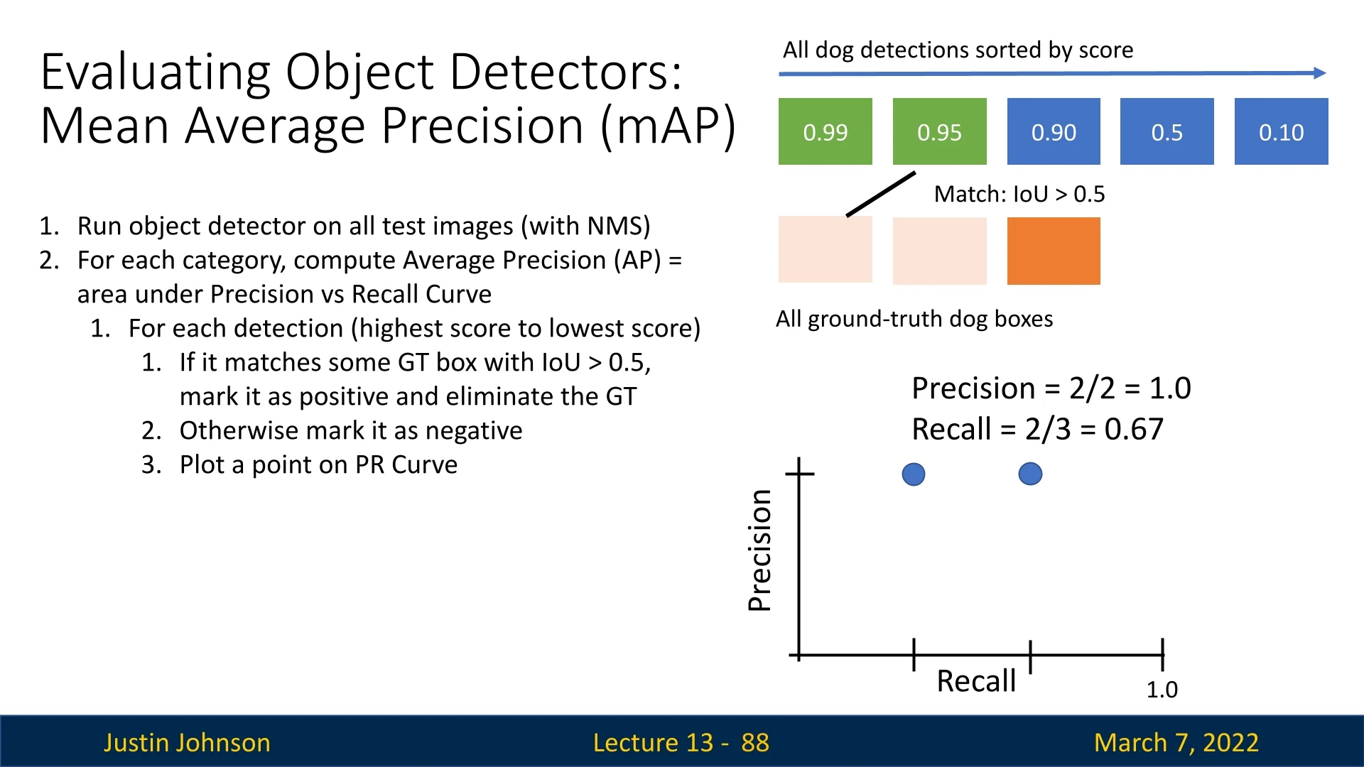
Figure 13.17: Step 2: Second match. The second highest detection correctly matches another ground-truth box. - 3.
- Third detection (score: 0.90): Does not match any ground-truth box
(False Positive).
- Precision = \( 2/3 \approx 0.67 \)
- Recall remains \( 2/3 \approx 0.67 \)
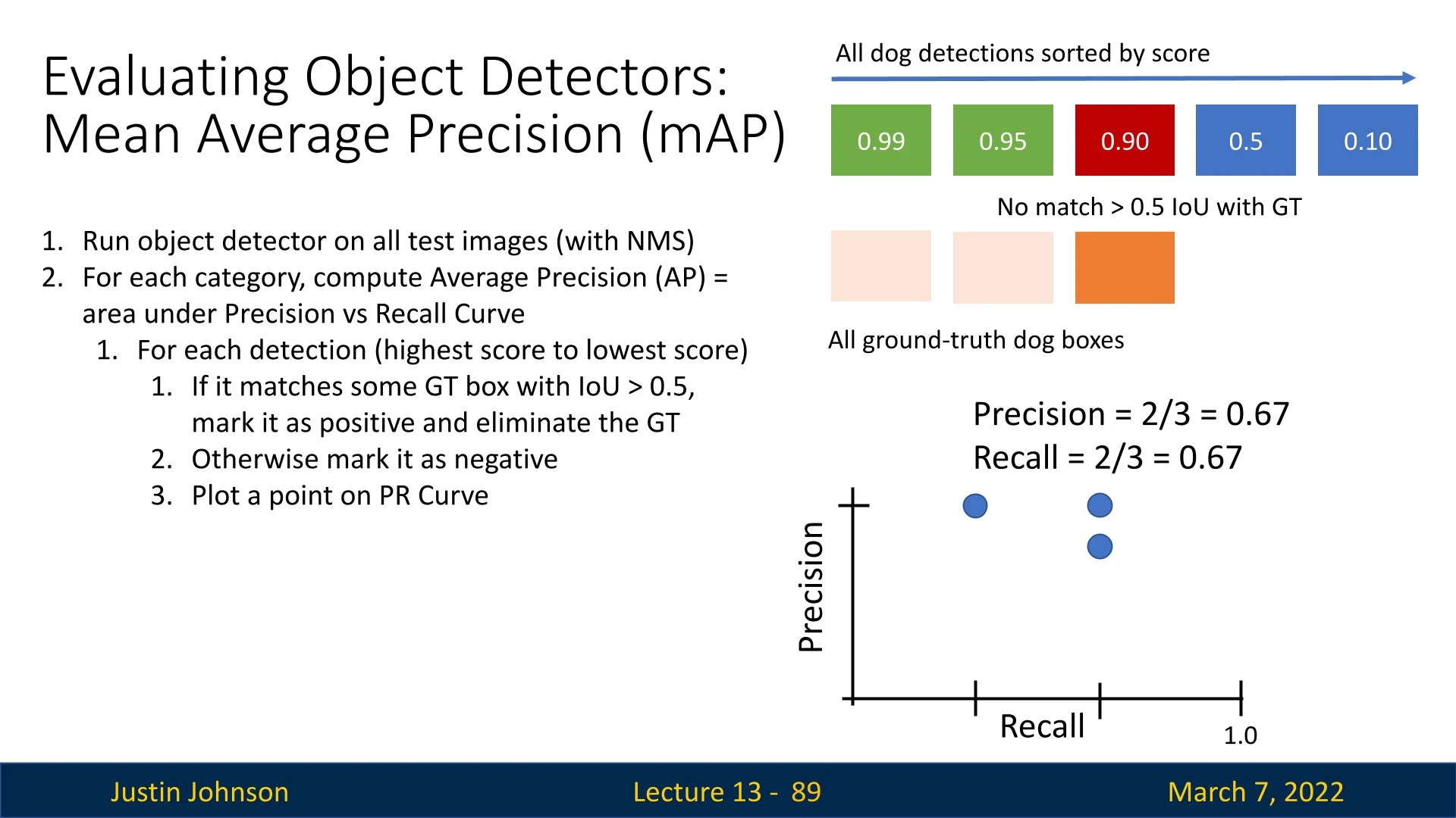
Figure 13.18: Step 3: False Positive. A detection fails to match any ground-truth box. - 4.
- Fourth detection (score: 0.85): Another false positive.
- Precision = \( 2/4 = 0.5 \)
- Recall remains \( 2/3 \approx 0.67 \)
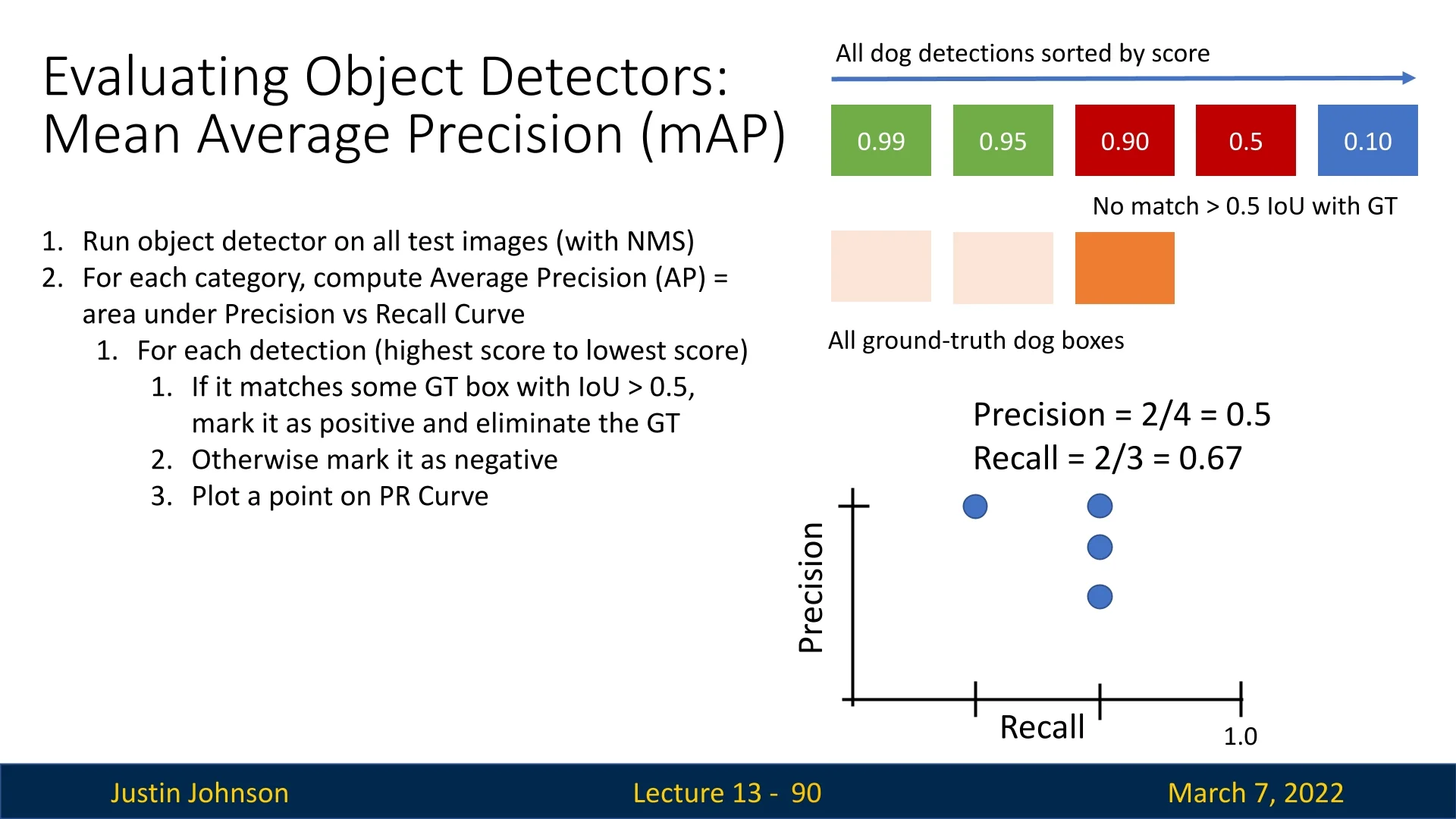
Figure 13.19: Step 4: Another False Positive. More false detections further lower precision. - 5.
- Final detection (score: 0.80): Matches the last ground-truth
box.
- Precision = \( 3/5 = 0.6 \)
- Recall = \( 3/3 = 1.0 \)
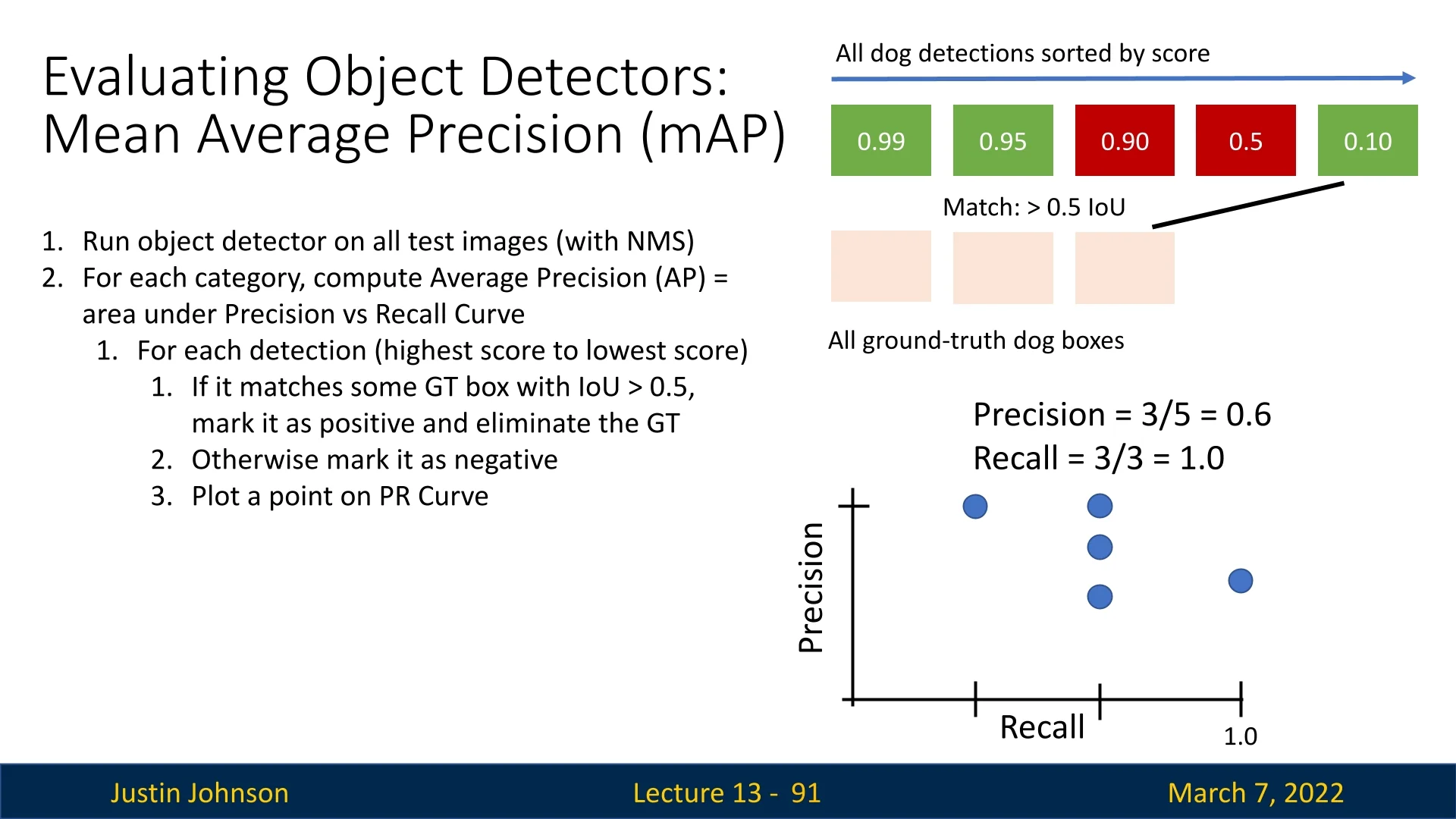
Figure 13.20: Final Step: All ground-truth boxes matched. Recall reaches 1.0, while the precision ends up being \(3/5=0.6\).
Final Result: The area under the PR curve, computed as AP@0.5, is 0.86.
13.5.3 Mean Average Precision (mAP)
To summarize performance across all object classes, we compute the mean Average Precision (mAP): \[ \mbox{mAP} = \frac {1}{N} \sum _{i=1}^{N} \mbox{AP}_i, \] where \( \mbox{AP}_i \) is the Average Precision for the \(i\)-th class, and \(N\) is the total number of classes. In our example, where we computed AP at an IoU threshold of 0.5 (i.e., AP@0.5), we have:
- \(\mbox{AP}_\mbox{dog} = 0.86\)
- \(\mbox{AP}_\mbox{cat} = 0.80\)
- \(\mbox{AP}_\mbox{car} = 0.65\)
Thus, \[ \mbox{mAP@0.5} = \frac {0.86 + 0.80 + 0.65}{3} \approx 0.77. \]
13.5.4 COCO mAP: A Stricter Measure
The COCO evaluation metric calculates mAP over a range of IoU thresholds—from 0.5 to 0.95 in increments of 0.05—as follows:
\[ \mbox{COCO mAP} = \frac {1}{10} \sum _{t=0.50}^{0.95} \mbox{AP}(t), \quad t \in \{0.50, 0.55, 0.60, \dots , 0.95\}. \]
By averaging AP values across multiple IoU thresholds, COCO mAP ensures that detectors not only identify objects but also localize them precisely. While traditional mAP@0.5 may accept loosely aligned bounding boxes, COCO mAP penalizes such cases by requiring consistently accurate localization across various levels of overlap. This makes it a more robust and stringent evaluation metric.
COCO mAP for Different Object Sizes
Object sizes in real-world scenarios can vary significantly, impacting detection performance. To capture this, the COCO evaluation framework computes mAP separately for different object scales:
- \( \mbox{COCO mAP}^\mbox{small} \) – Objects with an area \( < 32 \times 32 \) pixels.
- \( \mbox{COCO mAP}^\mbox{medium} \) – Objects with an area between \( 32 \times 32 \) and \( 96 \times 96 \) pixels.
- \( \mbox{COCO mAP}^\mbox{large} \) – Objects larger than \( 96 \times 96 \) pixels.
This breakdown is essential because different applications prioritize object sizes differently. Below is an example evaluation:
\[ \mbox{COCO mAP}^\mbox{small} = 0.25,\quad \mbox{COCO mAP}^\mbox{medium} = 0.45,\quad \mbox{COCO mAP}^\mbox{large} = 0.65. \]
When and Why Object Size-Specific mAP Matters Depending on the application, prioritizing specific object sizes is crucial:
-
Small Objects (\( \mbox{COCO mAP}^\mbox{small} \))
- Autonomous Vehicles: Detecting pedestrians at long distances is essential for safe driving.
- Aerial Surveillance: Drones must accurately detect small moving objects such as cars, people, or wildlife.
- Medical Imaging: Identifying small tumors in X-rays or CT scans can be life-saving.
-
Medium Objects (\( \mbox{COCO mAP}^\mbox{medium} \))
- Retail Analytics: Recognizing products on shelves in supermarkets.
- Autonomous Robotics: Object detection in warehouse management to identify items of various sizes.
- General-Purpose Security Systems: Detecting people and vehicles in surveillance footage.
-
Large Objects (\( \mbox{COCO mAP}^\mbox{large} \))
- Industrial Applications: Detecting machinery defects in large-scale manufacturing.
- Satellite Imagery: Identifying buildings, landscapes, and large infrastructure.
- Traffic Monitoring: Tracking entire vehicles or shipping containers in ports and highways.
Prioritizing Specific Classes in Object Detection
Beyond object sizes, many applications demand prioritization of specific classes. For example:
- Self-Driving Cars: Prioritizing pedestrians and stop signs over billboards and parked cars.
- Medical AI: Emphasizing cancerous lesions over benign anomalies.
- Surveillance Systems: Prioritizing human detection over objects like furniture.
To account for this, a weighted mAP can be used:
\[ \mbox{Weighted mAP} = \sum _{i} w_i \cdot \mbox{AP}_i, \quad \sum _{i} w_i = 1. \]
where \( w_i \) represents the importance weight for class \( i \). By applying different weights, we can ensure that models perform optimally for mission-critical object categories.
For instance, we might assign: \[ \begin {aligned} w_\mbox{Pedestrian} &= 0.4, \\ w_\mbox{Stop Sign} &= 0.3, \\ w_\mbox{Cyclist} &= 0.2, \\ w_\mbox{Billboard} &= 0.05, \\ w_\mbox{Parked Car} &= 0.05. \end {aligned} \] Using the Class AP values from the table: \[ \begin {aligned} \mbox{Weighted mAP} &= 0.4 \times 0.47 + 0.3 \times 0.72 + 0.2 \times 0.49 + 0.05 \times 0.34 + 0.05 \times 0.49 \\ &\approx 0.188 + 0.216 + 0.098 + 0.017 + 0.025 \\ &\approx 0.544. \end {aligned} \] Thus, the weighted mAP is approximately 0.54, aligning with the overall performance on mission-critical classes.
13.5.5 Evaluating Object Detectors: Key Takeaways
Object detection evaluation requires balancing classification accuracy and localization precision. Different metrics capture various aspects of model performance:
- AP measures a model’s ability to balance precision and recall using the area under the precision-recall curve.
- mAP extends AP by averaging it across object categories, providing a single metric for overall performance.
- COCO mAP improves upon standard mAP by averaging AP over multiple IoU thresholds (0.5 to 0.95), ensuring precise localization.
- Size-based COCO mAP evaluates performance on small, medium, and large objects, helping diagnose model weaknesses.
- Weighted mAP prioritizes critical object classes by assigning different importance weights, making evaluation more application-specific.
This structured approach ensures object detectors are evaluated fairly and optimized for the real-world tasks at hand. In the following parts of the document, we’ll discuss about improvements over the current R-CNN algorithm, improving both the computational overhead and speed of our object detection algorithms, along with enhanced algorithmic performance.
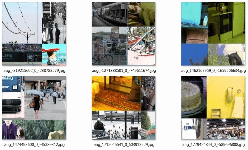
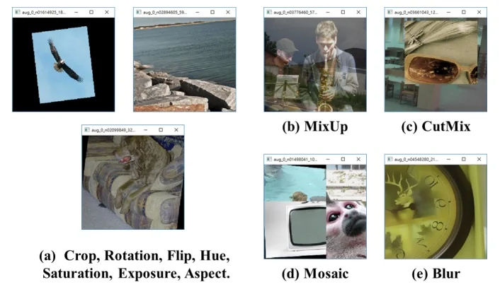
Enrichment 13.5.6: Mosaic Augmentation for Object Detection
While data augmentation techniques such as flipping, cropping, and jittering are widely used in classification, object detection introduces unique challenges: models must predict both what is in the image and where it is, using bounding boxes. This requires augmentations that preserve the structure and integrity of object locations. One popular strategy addressing this need is Mosaic augmentation, initially introduced in YOLOv4 [47] and later explored further in [84].
Motivation and Advantages Mosaic augmentation stitches together four different training images into a single \(2 \times 2\) grid, effectively constructing a new composite scene. This has several benefits:
- Scale Diversity: Objects are shown at smaller relative sizes, encouraging robustness to small object detection and training the model to recognize targets across varied resolutions.
- Context Enrichment: Different backgrounds and scene elements are juxtaposed, forcing the model to decouple object identity from a fixed or familiar context. This reduces overfitting to specific backgrounds and improves robustness to background variation at test time.
- Rare-Class Balancing: By combining object-centric and scene-centric images, Mosaic acts as a type of implicit upsampling for rare classes—helping combat class imbalance, particularly in long-tailed datasets.
Implementation Considerations Despite its power, Mosaic augmentation requires careful design:
- Coordinate Adjustment: Each original image’s bounding boxes must be re-mapped to their new locations in the mosaic coordinate system.
- Boundary Handling: Boxes crossing image seams should be clipped or filtered based on how much of the object remains visible.
- Semantic Noise: The abrupt visual seams between tiles may introduce low-level inconsistencies. While helpful for regularization, overly strong artifacts can confuse the network.
Domain-Dependent Utility Mosaic augmentation is particularly beneficial in domains where:
- Scenes contain multiple objects at varying scales.
- Small objects are common and must be localized accurately.
- Long-tailed class distributions are present.
- Robustness to background variation is essential, and training on fixed backgrounds might lead to context overfitting.
However, for tasks requiring precise geometric relationships (e.g., medical or industrial inspection), such artificial compositions might harm spatial reasoning and should be evaluated cautiously.
Advanced Usage and Scheduling in Modern Pipelines By construction, Mosaic produces highly synthetic training images that do not resemble the single-frame inputs used at inference time. As a result, modern real-time detectors rarely keep Mosaic active for the entire training run. Instead, Mosaic is used aggressively during an early or middle phase as a strong regularizer, and then disabled (or down-weighted) so that the model can refine on realistic images before convergence.
Concretely, DEIMv2 [257, 264] trains its S variant for 120 epochs but applies Mosaic only between epochs 4 and 64 with probability \(0.5\), and its ultra-lightweight variants train for 468 epochs while restricting Mosaic to epochs \(4\)–\(250\). This implements a “strong-then-mild” augmentation schedule: Mosaic drives robustness and small-object learning in the first half of training, and the last hundreds of epochs are devoted to polishing predictions on non-stitched images.
Similarly, RT-DETRv2 [418] adopts dynamic data augmentation, applying stronger augmentations early and then turning several of them off in the final epochs to better match the target domain. In the YOLO/Ultralytics ecosystem, Mosaic is controlled by a dedicated hyperparameter, and practical recipes often reduce this probability or set it to zero in the last stage of training so that the model sees only natural images near convergence [659].
Conclusion Mosaic augmentation extends traditional image-level augmentation into the object detection domain by combining multiple images into composite layouts. This promotes generalization to diverse backgrounds, improves small-object robustness, and implicitly balances class frequency. Furthermore, it enhances the model’s ability to distinguish foreground objects from noisy or unfamiliar backgrounds, reducing the risk of overfitting to scene context. In contemporary practice, Mosaic is typically used heavily during the first half of training and then disabled or down-weighted, allowing detectors such as DEIMv2 and RT-DETRv2 to fine-tune on realistic inputs before evaluation. More broadly, Mosaic exemplifies a key principle in deep learning: augmentation strategies must be tailored to the structure and demands of the task. Some tasks require additional domain-aware, label-preserving transformations, and effective augmentation therefore demands both creativity and a deep understanding of the task’s supervision signals and generalization requirements.