Lecture 17: Attention
17.1 Limitations of Sequence-to-Sequence with RNNs
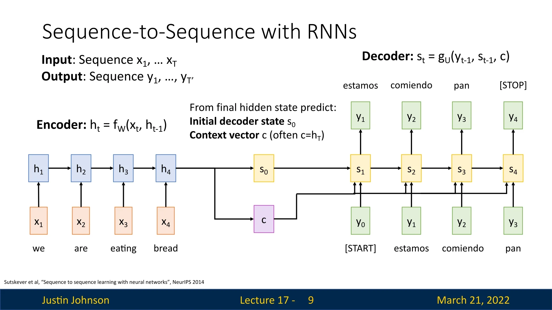
Previously, recurrent neural networks (RNNs) were used for sequence-to-sequence tasks such as machine translation. The encoder processed the input sequence and produced:
- A final hidden state \(s_0\), used as the first hidden state of the decoder network.
- A single, finite context vector \(c\) (often \(c = h_T\)), used at each step as input to the decoder.
The decoder then used \(s_0\) and \(c\) to generate an output sequence, starting with a <START> token and continuing until a <STOP> token was produced. The context vector \(c\) acted as a summary of the entire input sequence, transferring information from encoder to decoder.
While effective for short sequences, this approach faces issues when processing long sequences, as the fixed-size context vector \(c\) becomes a bottleneck, limiting the amount of information that can be retained and transferred.
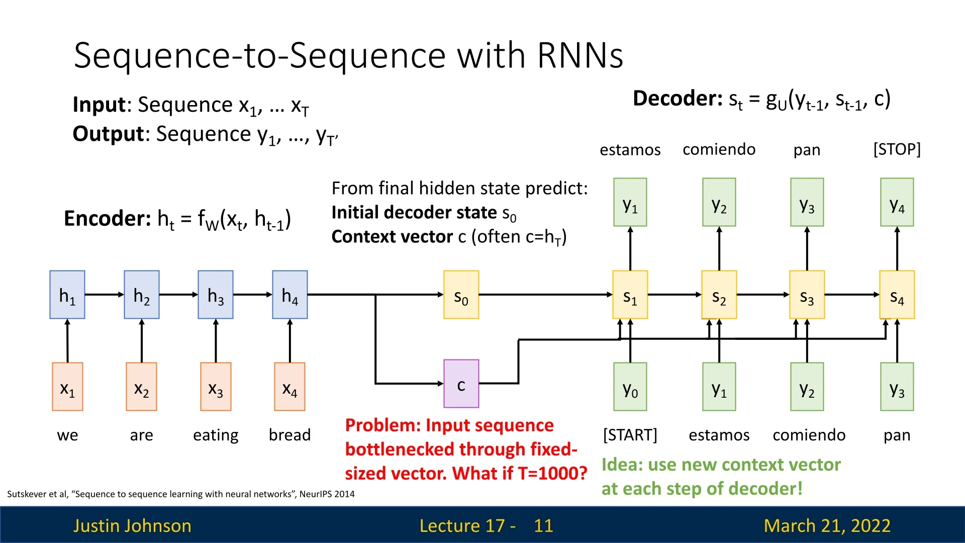
Even more advanced architectures like Long Short-Term Memory (LSTM) networks suffer from this issue because they still rely on the fixed-size \(c\) and \(h_T\) representations that do not scale with sequence length.
17.2 Introducing the Attention Mechanism
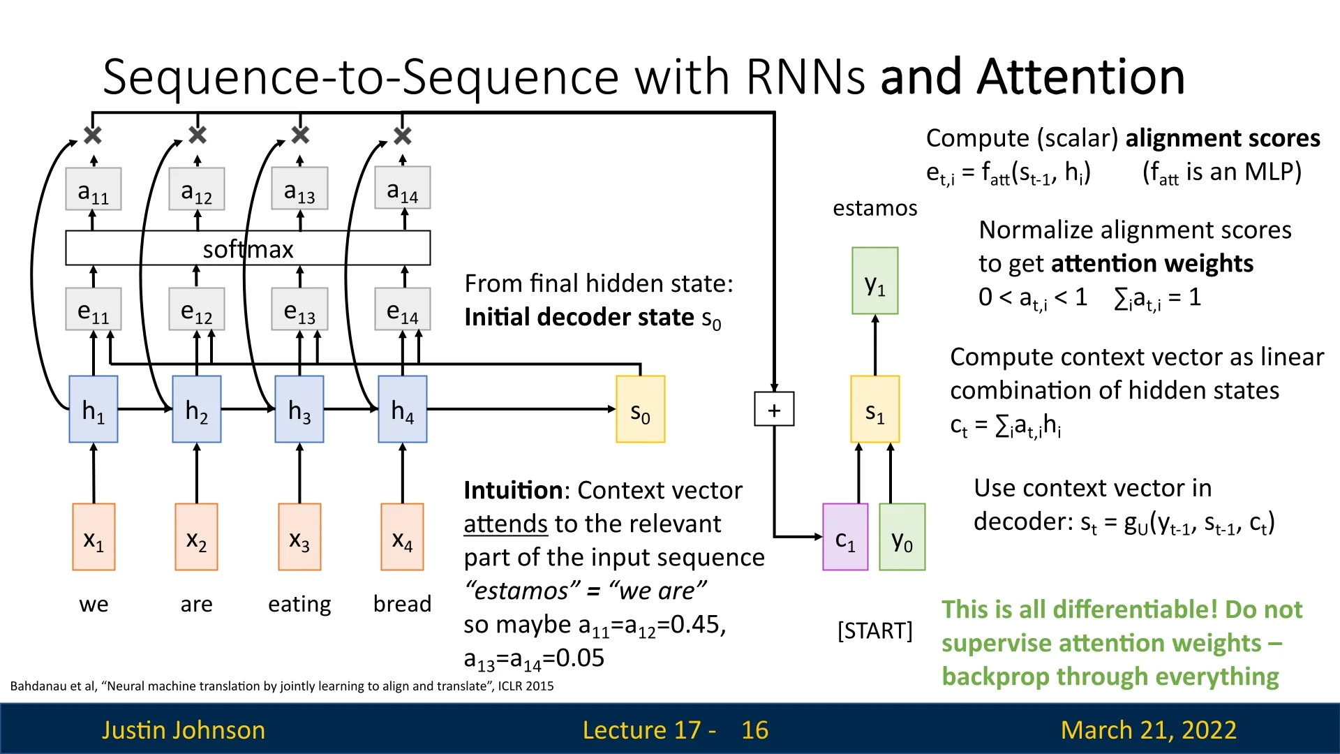
To address the bottleneck issue, the Attention mechanism introduces dynamically computed context vectors at each decoder step, instead of a single fixed vector. The encoder still processes the sequence to generate hidden states \(h_1, h_2, \dots , h_T\), but instead of passing only \(h_T\), an alignment function is used to determine which encoder hidden states are most relevant at each decoder step.
The key idea: Rather than using a single context vector for all decoder steps, the model computes a new context vector at each step by attending to different parts of the input sequence. This is done through a learnable alignment mechanism, historically known as additive attention or Bahdanau attention [22]:
\begin {equation} e_{t,i} = f_{att}(s_{t-1}, h_i), \end {equation} where \(f_{att}\) is a small, fully connected neural network. This function takes two inputs:
- The current hidden state of the decoder \(s_{t-1}\).
- A hidden state of the encoder \(h_i\).
By applying the function many times, over all encoder hidden states, it results in a set of alignment scores \(e_{t,1}, e_{t,2}, \dots , e_{t,T}\), where each score represents how relevant the corresponding encoder hidden state is to the current decoder step.
Applying the softmax function converts these alignment scores into attention weights: \begin {equation} a_{t,i} = \frac {\exp (e_{t,i})}{\sum _{j=1}^{T} \exp (e_{t,j})}, \end {equation} which ensures all attention weights are between \([0,1]\) and sum to \(1\).
The new context vector \(c_t\) is computed as a weighted sum of encoder hidden states: \begin {equation} c_t = \sum _{i=1}^{T} a_{t,i} h_i. \end {equation}
This means that at every decoding step, the decoder dynamically attends to different parts of the input sequence, adapting its focus based on the content being generated. Later in this chapter, we will contrast this additive, network-based scoring function with dot-product and scaled dot-product attention mechanisms, which replace \(f_{att}\) by simple inner products for improved computational efficiency in modern architectures such as Transformers.
Intuition Behind Attention
Instead of relying on a single compressed context vector, attention allows the model to focus on the most relevant parts of the input sequence dynamically. For example, when translating "we are eating bread" to "estamos comiendo pan", the attention weights at the first step might be: \begin {equation} a_{11} = a_{12} = 0.45, \quad a_{13} = a_{14} = 0.05. \end {equation} This means the model places greater emphasis on the words "we are" when producing "estamos", and will shift attention accordingly as it generates more words.
17.2.1 Benefits of Attention
Attention mechanisms improve sequence-to-sequence models in several ways:
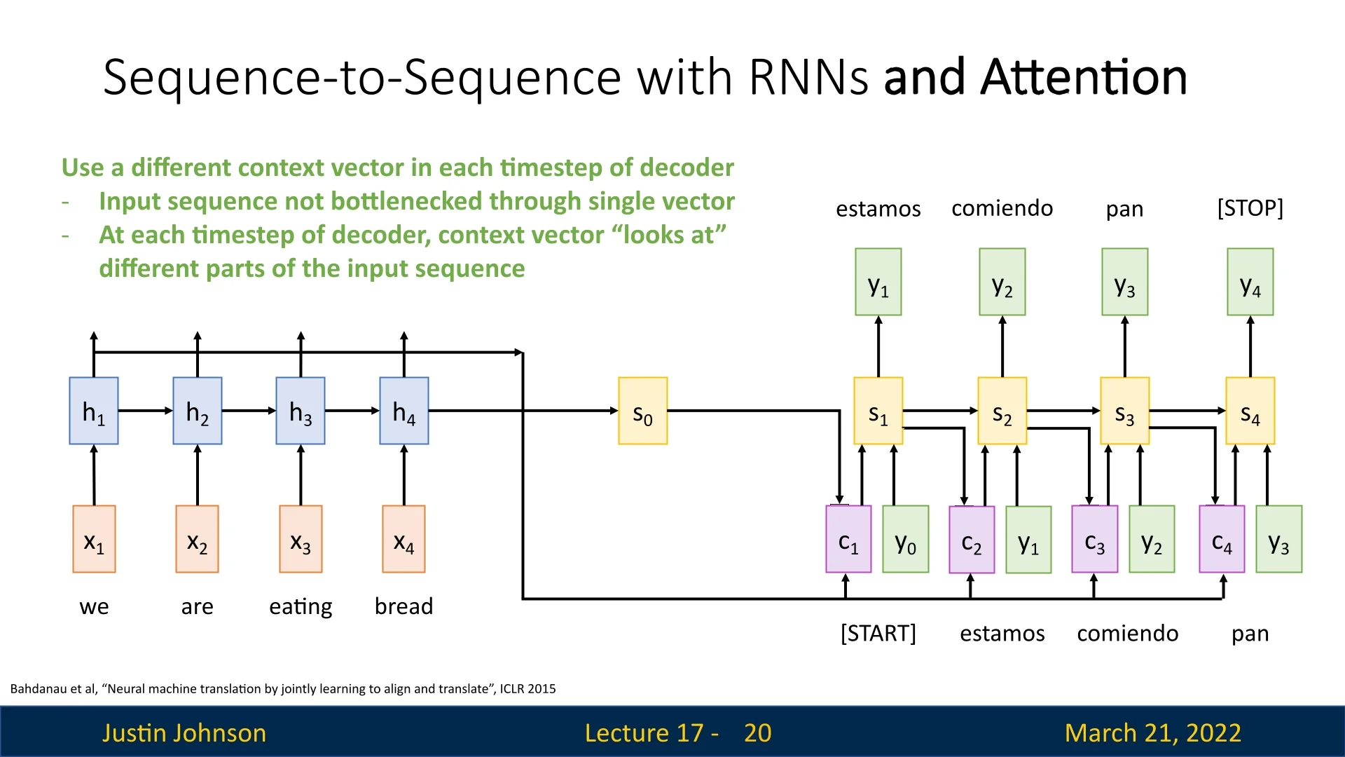
- Eliminates the bottleneck: The input sequence is no longer constrained by a single fixed-size context vector.
- Dynamic focus: Each decoder step attends to different parts of the input, rather than relying on a static summary.
- Improved alignment: The model learns to associate corresponding elements in input and output sequences automatically.
Additionally, attention mechanisms are fully differentiable, meaning they can be trained end-to-end via backpropagation without explicit supervision of attention weights.
17.2.2 Attention Interpretability
The introduction of attention mechanisms has revolutionized sequence-to-sequence learning by addressing the limitations of a fixed-size context vector. Rather than relying on a static summary of the input, attention dynamically selects relevant information at each decoding step, significantly improving performance on long sequences and enabling models to learn meaningful alignments between input and output sequences.
One of the key advantages of attention is its interpretability. By visualizing attention maps, we can gain deeper insight into how the model aligns different parts of the input with the generated output. These maps illustrate how the network distributes its focus across the input sequence at each step, offering a way to diagnose errors and refine architectures for specific tasks.
Attention Maps: Visualizing Model Decisions
A particularly interesting property of attention is that it provides an interpretable way to analyze how different parts of the input sequence influence each predicted output token. This is achieved through attention maps, which depict the attention weights as a structured matrix.
To see this in action, let us revisit our sequence-to-sequence translation example, but now translating from English to French using the attention mechanism proposed by Bahdanau et al. [22]. Consider the following English sentence:
‘‘The agreement on the European Economic Area was signed in August 1992 . <end>’’
which the model translates to French as:
‘‘L’accord sur la zone économique européenne a été signé en août 1992 . <end>’’
By constructing a matrix of size \(T' \times T\) (where \(T'\) is the number of output tokens and \(T\) is the number of input tokens), we can visualize the attention weights \(a_{i,j}\), which quantify how much attention the decoder assigns to each encoder hidden state when generating an output token. A higher weight corresponds to a stronger influence of the encoder hidden state \(h_j\) on the decoder state \(s_i\), which then produces the output token \(y_i\).
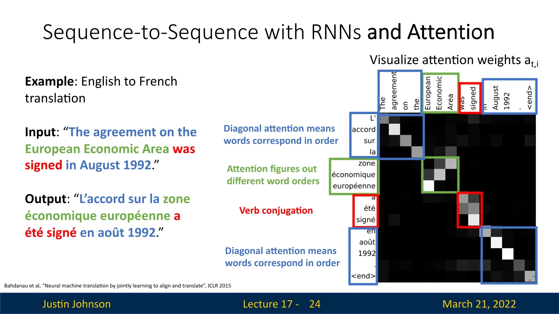
In this visualization, each cell represents an attention weight \(a_{i,j}\), where a brighter color corresponds to a higher weight (i.e., stronger attention), and a darker color corresponds to a lower weight (weaker attention). The map reveals how the model distributes its focus while generating each output word.
Understanding Attention Patterns
Observing the attention map, we notice an almost diagonal alignment. This makes sense, as words in one language typically correspond to words in the other in the same order. For example, the English word ‘‘The’’ aligns with the French ‘‘L’ ’’, and ‘‘agreement’’ aligns with ‘‘accord’’. This pattern suggests that the model has learned a reasonable alignment between source and target words.
However, not all words align perfectly in the same order. Some phrases require reordering due to syntactic differences between languages. A notable example is the phrase:
‘‘European Economic Area’’ \(\rightarrow \) ‘‘zone économique européenne’’
Here, the attention map reveals that the model adjusts its focus dynamically, attending to different words at different decoding steps. In English, adjectives precede nouns, while in French, they follow. The attention map correctly assigns a higher weight to ‘‘zone’’ when generating the French ‘‘zone’’, then shifts attention to ‘‘economic’’ and ‘‘European’’ at appropriate steps.
This behavior shows that the model is not merely copying words but has learned meaningful language structure. Importantly, we did not explicitly tell the model these word alignments—it learned them from data alone. The ability to extract these patterns purely from training data without human supervision is a major advantage of attention-based architectures.
Why Attention Interpretability Matters
The interpretability provided by attention maps allows us to:
- Understand model predictions: By visualizing attention distributions, we can verify whether the model is focusing on the right input words for each output token.
- Debug model errors: If a translation error occurs, the attention map can reveal whether it was due to misaligned attention weights.
- Gain linguistic insights: The learned alignments sometimes uncover grammatical and syntactic relationships across languages that may not be immediately obvious.
This ability to interpret how neural networks make decisions was largely missing from previous architectures, making attention a crucial development in deep learning. As we move forward, we will explore even more advanced forms of attention, such as self-attention in Transformers, which allows models to process entire sequences in parallel rather than sequentially.
17.3 Applying Attention to Image Captioning
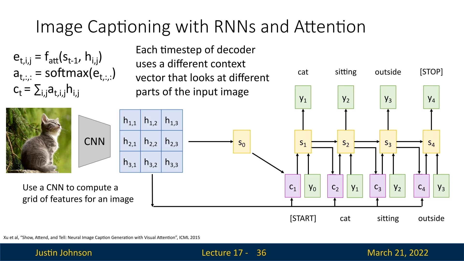
The flexibility of attention mechanisms—in particular, their ability to operate on unordered sets of vectors—allows them to extend naturally from text-based sequence modeling to computer vision tasks such as image captioning. This was demonstrated in the seminal work by Xu et al. [732], “Show, Attend and Tell: Neural Image Caption Generation with Visual Attention”. Rather than compressing an entire image into a single fixed-size feature vector, their model uses an attention-based decoder that dynamically focuses on different image regions while generating each word of the caption.
17.3.1 Feature Representation
The input image is first processed by a convolutional neural network (CNN), and we extract a convolutional feature map of shape \(C_{\mbox{out}} \times H' \times W'\). Instead of treating this as a single global vector, we flatten the spatial dimensions to obtain a set of \(L = H' W'\) feature vectors \[ A = \{ h_1, \dots , h_L \}, \quad h_i \in \mathbb {R}^{C_{\mbox{out}}}. \] Each vector \(h_i\) corresponds to a specific receptive field in the original image and serves as a spatial annotation.
These vectors play the same role as the encoder hidden states \(\{h_1, \dots , h_T\}\) in sequence-to-sequence models: they form an unordered set over which the decoder can apply attention. The goal of the attention mechanism is to construct, at each decoding step, a context vector \(c_t\) that selectively aggregates information from these spatial features.
17.3.2 Attention-Based Caption Decoder
The caption is generated one token at a time by a recurrent decoder (for example, an LSTM) equipped with additive (Bahdanau) attention over the image features.
Initialization Before generation begins, the decoder needs an initial hidden state \(s_0\) that summarizes the overall content of the image.
Rather than initializing \(s_0\) from a special token, we compute it from the spatial features using a small MLP \(g_{\mbox{init}}\): \begin {equation} s_0 = g_{\mbox{init}}\!\left (\frac {1}{L} \sum _{i=1}^{L} h_i \right ). \end {equation} This provides a global, learned summary of the image that grounds the decoding process.
Additive attention and context computation At each timestep \(t\), the decoder maintains a hidden state \(s_{t-1}\) and has access to the image features \(\{h_i\}\). It uses the same additive attention function \(f_{att}\) introduced earlier to compute alignment scores between the current state and each image region: \begin {equation} e_{t,i} = f_{att}(s_{t-1}, h_i). \end {equation} Recall that in additive (Bahdanau) attention, \(f_{att}\) is implemented as a shallow MLP that projects \(s_{t-1}\) and \(h_i\) into a shared space and scores their compatibility; a common choice is \begin {equation} e_{t,i} = v_a^{\top } \tanh (W_a s_{t-1} + U_a h_i), \end {equation} with learnable parameters \(W_a, U_a, v_a\).
These alignment scores are normalized with a softmax to obtain attention weights over all spatial locations: \begin {equation} \alpha _{t,i} = \frac {\exp (e_{t,i})}{\sum _{k=1}^{L} \exp (e_{t,k})}, \end {equation} where \(\alpha _{t,i}\) indicates how strongly the decoder attends to region \(i\) at timestep \(t\).
The context vector \(c_t\) is then computed as the corresponding weighted sum of the spatial features: \begin {equation} c_t = \sum _{i=1}^{L} \alpha _{t,i} h_i. \end {equation}
State update and word prediction Given the previous word \(y_{t-1}\), the previous hidden state \(s_{t-1}\), and the newly computed context vector \(c_t\), the decoder updates its state and predicts the next word: \begin {align} s_t &= \text {RNN}(s_{t-1}, [y_{t-1}, c_t]), \\ p(y_t \mid y_{<t}, \text {image}) &\propto \exp \big (L_o(s_t, c_t)\big ), \end {align}
where \(L_o\) is a learned output layer (typically a linear layer followed by a softmax over the vocabulary). This procedure repeats until the decoder emits the <END> token.
Example: “cat sitting outside” In Figure 17.6, the caption generated for the image is
<START> cat sitting outside <STOP>.
At \(t=1\), when predicting cat, the attention weights \(\{\alpha _{1,i}\}\) typically concentrate on the region containing the cat. At \(t=2\), for sitting, the model continues to focus on the cat but may shift towards regions that reveal posture (such as the body and the surface it sits on). By \(t=3\), when producing outside, attention can expand toward the background, emphasizing regions that signal the outdoor environment (trees, grass, or sky). The caption thus emerges from a sequence of content-dependent glimpses over the image, rather than from a single static global representation.
17.3.3 Visualizing Attention in Image Captioning
As in the translation examples earlier in this chapter, attention weights in image captioning can be visualized as spatial attention maps, revealing where the model “looks” when generating each word. Figure 17.7 illustrates this interpretability for the caption
‘‘A bird flying over a body of water .’’
generated by an attention-based image captioning model.
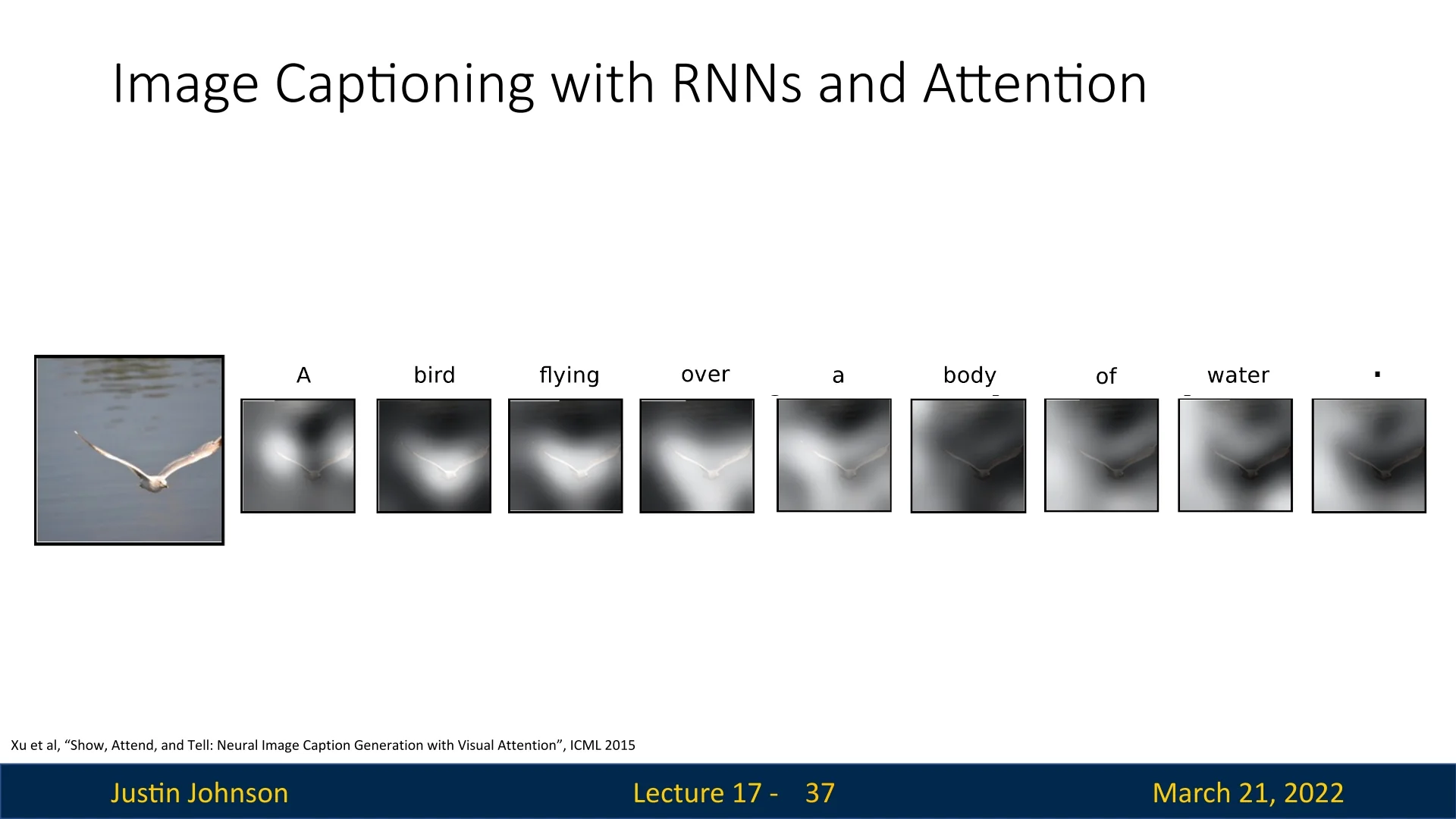
Reading the sequence of maps from left to right, we can see how the model’s focus shifts over the image as the caption unfolds:
- For function words such as A or of, the attention is relatively diffuse, reflecting that these tokens are driven more by language modeling than by specific visual evidence.
- When predicting the noun bird, the attention weights concentrate on the pixels covering the bird, grounding the object word in the correct region of the image.
- For the verb flying, the model continues to focus on the bird—particularly around its body and wings—since the action is attributed to that object.
- When generating water, the attention shifts away from the bird and spreads over the lower part of the image corresponding to the water surface, capturing the background context needed to complete the phrase ‘‘a body of water’’.
These maps provide a direct, spatially grounded view of how the model aligns words with image regions. They are produced by the soft attention mechanism described above, in which the model maintains a differentiable distribution \(\{\alpha _{t,i}\}\) over all spatial locations at each timestep. Xu et al. [732] also explore a hard attention variant that samples a single region per timestep; while potentially more efficient, this discrete sampling is not differentiable and therefore requires reinforcement-learning techniques (such as REINFORCE) for training.
17.3.4 Biological Inspiration: Saccades in Human Vision
An interesting question we can ask ourselves is: How similar is this mechanism to how humans perceive the world? As it turns out, the resemblance is quite significant.
The retina, the light-sensitive layer inside our eye, is responsible for converting incoming light into neural signals that our brain processes. However, not all parts of the retina contribute equally to our vision. The central region, known as the fovea, is a specialized area that provides high-acuity vision but covers only a small portion of our total visual field.
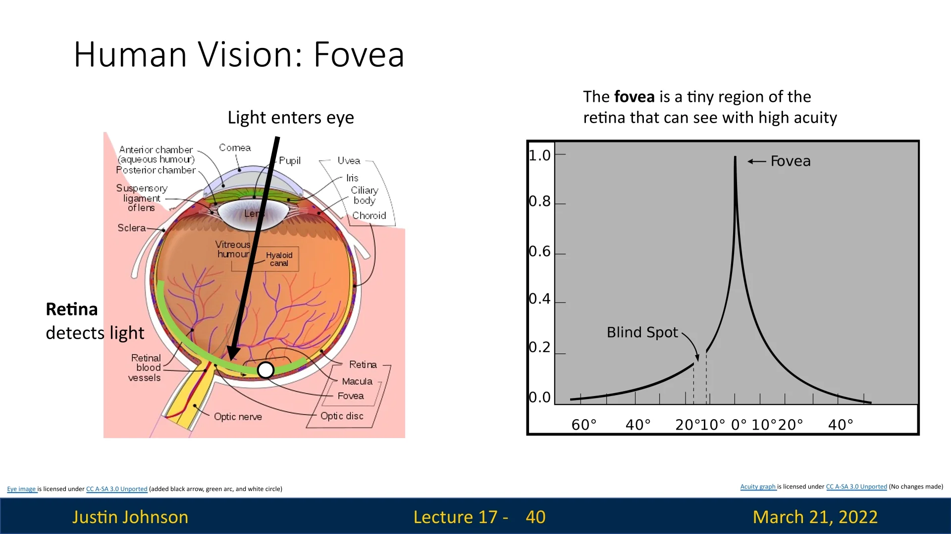
As seen in Figure 17.8, only a small region of the retina provides clear, detailed vision. The rest of our visual field consists of lower-resolution perception. To compensate for this, human eyes perform rapid, unconscious movements called saccades, dynamically shifting the fovea to different areas of interest in a fraction of a second.
Attention-based image captioning mimics this biological mechanism. Just as our eyes adjust their focus to capture different parts of a scene, attention in RNN-based captioning models selectively attends to different image regions at each timestep. The model does not process the entire image at once; instead, it dynamically ”looks” at relevant portions as it generates each word in the caption.
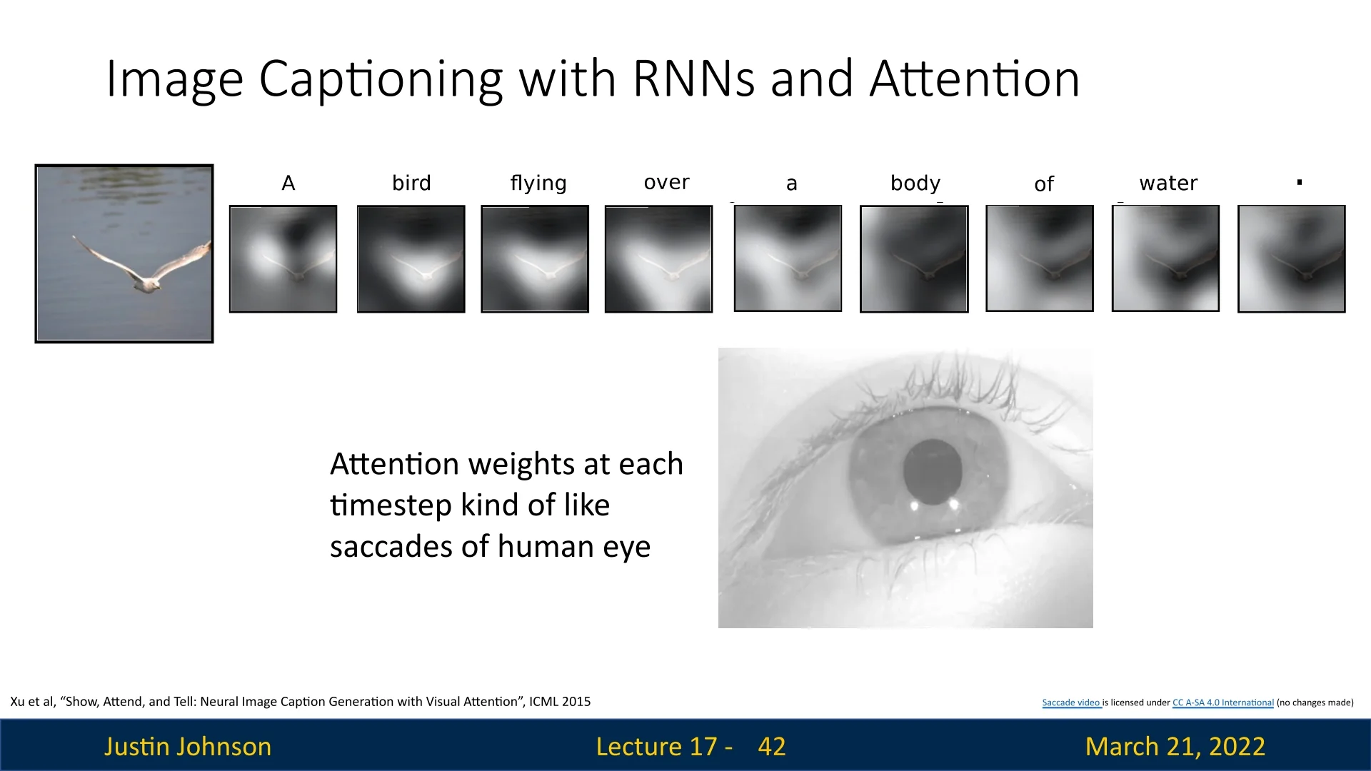
In Figure 17.9, we can see how attention weights at each timestep act like saccades in the human eye. Rather than maintaining a static focus, the model dynamically shifts its attention across different image regions, much like our eyes scan a scene.
Key parallels between saccades and attention-based image captioning:
- Selective focus: Human vision relies on the fovea to process high-resolution details, while peripheral vision provides contextual information. Similarly, attention assigns higher weights to relevant image regions while keeping a broader, low-weighted awareness of the rest.
- Dynamic adjustment: Just as saccades allow humans to explore different parts of a scene, attention-based models shift focus across image regions as new words are generated.
- Efficient processing: The brain does not process an entire scene at once; instead, it strategically selects important details. Attention mechanisms follow the same principle by prioritizing certain regions rather than treating all pixels equally.
This biological inspiration helps explain why attention mechanisms are so effective in vision tasks—they leverage a principle that human perception has refined over millions of years. The next section will explore how this interpretability can be visualized through attention maps.
17.3.5 Beyond Captioning: Generalizing Attention Mechanisms
The power of attention extends beyond image captioning. Inspired by ”Show, Attend, and Tell,” numerous works have applied similar mechanisms to diverse tasks:
- Visual Question Answering (VQA) [731]: Attend to image regions relevant to answering a given question.
- Speech Recognition [75]: Attend to audio frames while generating text transcriptions.
- Robot Navigation [433]: Attend to textual instructions to guide robotic movement.
These applications demonstrate that attention is not merely a tool for sequential processing—it is a powerful and general framework for learning relationships between different modalities. This leads naturally to the development of Attention Layers, which we will explore next.
17.4 Attention Layer
In computer science, when a method proves broadly useful, the natural progression is to abstract and generalize it into a reusable module. This principle applies to attention. What began as a task-specific technique for encoder–decoder RNNs was distilled into a general-purpose Attention Layer that can be integrated across architectures and domains.
To move from the original “RNN + Attention” setting to a modular view, we replace task-specific names with generic roles:
- Query vector \(q\): the vector that asks “what is relevant now?” In encoder–decoder RNNs, this is typically the decoder state \(s_{t-1}\), with shape \(D_Q\).
- Input vectors \(X = \{X_i\}_{i=1}^{N_X}\): the set of vectors we may attend to. These could be encoder states \(h_i\) in translation or spatial CNN features \(h_{i,j}\) in vision, with shape \(N_X \times D_X\).
- Similarity function \(f_{\mbox{att}}\): a scoring rule that measures compatibility between \(q\) and each \(X_i\). Early attention mechanisms used a small MLP (additive/Bahdanau attention), while modern architectures often use dot-product-based scoring.
Regardless of the domain, the attention computation follows the same three-step template:
- 1.
- Compute similarities: \begin {equation} e_i = f_{\mbox{att}}(q, X_i), \quad e \in \mathbb {R}^{N_X}. \end {equation}
- 2.
- Normalize weights: \begin {equation} a_i = \frac {\exp (e_i)}{\sum _j \exp (e_j)}. \end {equation}
- 3.
- Aggregate inputs: \begin {equation} y = \sum _{i} a_i X_i. \end {equation}
The attention layer formalizes this pattern as a standard building block that takes a query and a set of input vectors and returns an attended output. A natural next question is which scoring function \(f_{\mbox{att}}\) provides the best balance of expressivity, efficiency, and optimization stability.
17.4.1 Scaled Dot-Product Attention
In the earlier RNN-based formulations, the similarity function \(f_{\mbox{att}}\) was implemented as a small MLP: \begin {equation} e_i = f_{\mbox{att}}(q, x_i) = v_a^{\top }\tanh (W_a q + U_a x_i), \end {equation} which is known as additive (Bahdanau) attention. This learned scoring network is flexible, but it introduces additional parameters and per-pair nonlinear computation.
Modern attention architectures, most notably the Transformer, simplify this step. They replace the MLP with a direct geometric similarity and add a principled normalization: \begin {equation} e_i = \frac {\mathbf {q} \cdot \mathbf {x}_i}{\sqrt {D_Q}}, \qquad \mathbf {q}\in \mathbb {R}^{D_Q}, \quad \mathbf {x}_i\in \mathbb {R}^{D_Q}. \end {equation} Thus, \begin {equation} f_{\mbox{att}}(q, x_i) = \frac {q^{\top }x_i}{\sqrt {D_Q}}, \end {equation} meaning that the learned MLP used in additive attention is replaced by a simple dot product. The dot product measures how well aligned the two vectors are in the embedding space, and the scaling term controls the magnitude of the resulting logits before softmax.
Why Scale by \(\sqrt {D_Q}\)? At first glance, dividing by \(\sqrt {D_Q}\) may look like a technical detail. In practice, it is crucial for stable training.
1. Why does the dot-product variance grow with dimension? Write the unscaled dot product as a sum of coordinate-wise products: \begin {equation} \mathbf {q}\cdot \mathbf {x}_i \;=\; \sum _{d=1}^{D_Q} q_d\,x_{i,d}. \end {equation} Assume, as a simplifying heuristic, that \(q_d\) and \(x_{i,d}\) are independent, zero-mean, and identically distributed with variance \(\sigma ^2\). Then each product term has \begin {equation} \mathbb {E}[q_d x_{i,d}] = 0, \qquad \mbox{Var}(q_d x_{i,d}) = \mathbb {E}[q_d^2 x_{i,d}^2] = \mathbb {E}[q_d^2]\mathbb {E}[x_{i,d}^2] = \sigma ^4. \end {equation} If we further assume these product terms are approximately independent across \(d\), then the variance of the sum grows linearly: \begin {equation} \mbox{Var}[\,\mathbf {q}\cdot \mathbf {x}_i\,] \;\approx \; D_Q \sigma ^4. \end {equation} Thus, the standard deviation of the raw dot product scales like \(\sqrt {D_Q}\). In high-dimensional models (e.g., \(D_Q = 512\) or \(1024\)), this naturally produces larger-magnitude logits.
2. Why are large magnitudes a problem for softmax? After computing scores, we normalize them with softmax: \begin {equation} a_i \;=\; \frac {\exp (e_i)}{\sum _{j=1}^{N_X} \exp (e_j)}. \end {equation} When one score is much larger than the others, \(\exp (e_i)\) overwhelms the denominator. The resulting attention distribution becomes nearly one-hot.
A small numerical example makes this concrete. With modest logits, \[ \mbox{softmax}([2,1]) \approx [0.73,\,0.27], \] the distribution is “soft,” so gradients can meaningfully adjust both scores. But if the logits are scaled up, \[ \mbox{softmax}([20,10]) \approx [0.99995,\,0.00005], \] softmax effectively behaves like an \(\texttt{argmax}\). In this saturated regime, the gradient of softmax becomes extremely small. Consequently, the model stops learning because the error signal cannot backpropagate through these saturated regions.
3. How does scaling fix this? Dividing by \(\sqrt {D_Q}\) counteracts the growth in logit magnitude: \begin {equation} e_i \;=\; \frac {\mathbf {q}\cdot \mathbf {x}_i}{\sqrt {D_Q}} \quad \Longrightarrow \quad \mbox{Var}[\,e_i\,] \;\approx \; \sigma ^4, \end {equation} so the typical scale of the scores remains roughly stable as \(D_Q\) increases. This keeps softmax in a regime where the attention distribution is neither too sharp nor too flat, preserving healthy gradients and improving optimization.
Scaling and softmax temperature Softmax is invariant to adding a constant to all logits, but it is not invariant to scaling. We can interpret the normalization by \(\sqrt {D_Q}\) as a principled temperature control: \begin {equation} a_i \;=\; \frac {\exp (e_i / T)}{\sum _{j} \exp (e_j / T)}. \end {equation} If the effective temperature is too low, attention becomes overly peaked and brittle. If it is too high, attention becomes nearly uniform and loses discriminative power. The \(\sqrt {D_Q}\) scaling is a robust default that keeps attention well-calibrated across model widths.
Why dot product? Replacing additive attention with scaled dot-product attention offers several advantages:
- Compute efficiency: Dot products can be implemented as batched matrix multiplications, which are highly optimized on modern accelerators [664].
- Parameter efficiency: The scoring step introduces no additional MLP parameters, unlike additive attention [22].
- Competitive accuracy: Despite its simplicity, scaled dot-product attention matches or surpasses MLP-based scoring in large-scale sequence modeling benchmarks [22, 664].
In summary, scaled dot-product attention replaces the learned MLP similarity function of additive attention with a simpler inner product, while using \(\sqrt {D_Q}\) scaling to maintain stable, trainable softmax behavior. This combination of efficiency and stability is a key reason it became the default scoring rule in modern attention layers.
In the next part, we will extend this single-query formulation to multiple query vectors computed in parallel, enabling a compact matrix form of attention that directly sets up self-attention and Transformer blocks.
From a single query to many queries So far, we have described attention for a single query vector \(q\). In practice, we almost always need to process multiple queries in parallel. In the next part, we will generalize this formulation to a set of queries \( Q \in \mathbb {R}^{N_Q \times D_Q} \) attending over an input set \( X \in \mathbb {R}^{N_X \times D_Q}, \) and we will express the entire computation as efficient matrix operations: \[ \mbox{Attention}(Q, X) \;=\; \mbox{softmax}\!\left (\frac {QX^{\top }}{\sqrt {D_Q}}\right )X. \] This multi-query view is the direct bridge to self-attention and the Transformer blocks we will develop next.
17.4.2 Extending to Multiple Query Vectors
Given a query matrix \( Q \in \mathbb {R}^{N_Q \times D_Q} \), we compute attention scores in parallel:
\begin {equation} E = \frac {Q X^T}{\sqrt {D_Q}}, \quad E \in \mathbb {R}^{N_Q \times N_X}. \end {equation}
We then apply the softmax function along the input dimension to normalize attention scores:
\begin {equation} A = \mbox{softmax}(E), \quad A \in \mathbb {R}^{N_Q \times N_X}. \end {equation}
The final attention-weighted output is obtained by computing: \begin {equation} Y = A X, \quad Y \in \mathbb {R}^{N_Q \times D_X}. \end {equation}
- Parallel Computation: Multiple queries benefit from the efficient processing through matrix-matrix multiplications of scaled-dot product self-attention. Hence, we can use them to increase our per-layer representational capacity.
- Richer Representations: Allows capturing diverse relationships between inputs and queries.
- Token-Wise Attention: Essential for self-attention layers (covered later), where each token in a sequence attends to others independently.
17.4.3 Introducing Key and Value Vectors
In early formulations, the input vectors \( X \) were used both to compute attention scores and to generate outputs. However, these two functions serve distinct purposes:
- Keys (\( K \)) determine how queries interact with different input elements.
- Values (\( V \)) contain the actual information retrieved by attention.
Instead of using \( X \) directly, we introduce learnable weight matrices (transformations):
\begin {equation} K = X W_K, \quad K \in \mathbb {R}^{N_X \times D_Q}, \quad V = X W_V, \quad V \in \mathbb {R}^{N_X \times D_V}. \end {equation}
The attention computation is then reformulated as:
\begin {equation} E = \frac {Q K^T}{\sqrt {D_Q}}, \quad A = \mbox{softmax}(E), \quad Y = A V. \end {equation}
- Decouples Retrieval from Output Generation: Keys optimize for similarity matching, while values store useful information.
- Increased Expressiveness: Independent key-value transformations improve model flexibility.
- Efficient Memory Access: Enables retrieval-like behavior, where queries search for relevant information rather than being constrained by input representations.
17.4.4 An Analogy: Search Engines
Attention mechanisms can be understood through the analogy of a search engine, which retrieves relevant information based on a user query. In this analogy:
- Query: The search phrase entered by the user.
- Keys: The indexed metadata linking queries to stored information.
- Values: The actual content retrieved in response to the query.
Just as a search engine compares a query to indexed keys but returns values, attention mechanisms compute query-key similarities to determine which values contribute to the final output.
Empire State Building Example
Consider the query "How tall is the Empire State Building?":
- 1.
- The search engine identifies relevant terms from the query.
- 2.
- It retrieves indexed keys, such as "Empire State Building" and "building height".
- 3.
- It selects pages containing the most relevant values, such as "The Empire State Building is 1,454 feet tall, including its antenna.".
Similarly, attention mechanisms:
- Use query vectors to determine information needs.
- Compare them to key vectors to identify relevant input.
- Retrieve value vectors to generate the final output.
Why This Separation Matters
Separating queries, keys, and values provides:
- Efficiency: Enables fast retrieval without processing all inputs sequentially.
- Flexibility: Allows different queries to focus on various input aspects.
- Generalization: Adapts across tasks without modifying the entire model.
17.4.5 Bridging to Visualization and Further Understanding
Visualizing attention enhances understanding. Below, we outline the steps of the Attention Layer and explain how its structure facilitates interpretation.
Overview of the Attention Layer Steps
The attention mechanism follows a structured sequence of computations:
- 1.
- Inputs to the Layer: The layer receives a set of query vectors \( Q \) and a set of input vectors \( X \). In our example: \begin {equation} Q = \{Q_1, Q_2, Q_3, Q_4\}, \quad X = \{X_1, X_2, X_3\}. \end {equation}
- 2.
- Computing Key Vectors: Each input vector \( X_i \) is transformed into a key vector \( K_i \) using the learnable key matrix \( W_K \): \begin {equation} K = X W_K, \quad K \in \mathbb {R}^{N_X \times D_Q}. \end {equation} In our example, we obtain: \begin {equation} K = \{K_1, K_2, K_3\}, \quad \mbox{where } K_i = X_i W_K. \end {equation}
- 3.
- Computing Similarities: Each query vector is compared to all key vectors using the scaled dot product: \begin {equation} E = \frac {QK^T}{\sqrt {D_Q}}, \quad E \in \mathbb {R}^{N_Q \times N_X}. \end {equation} The resulting matrix \( E \) contains unnormalized similarity scores, where each row corresponds to a query vector and each column corresponds to a key vector: \begin {equation} E = \begin {bmatrix} E_{1,1} & E_{1,2} & E_{1,3} \\ E_{2,1} & E_{2,2} & E_{2,3} \\ E_{3,1} & E_{3,2} & E_{3,3} \\ E_{4,1} & E_{4,2} & E_{4,3} \end {bmatrix}. \end {equation} Here, \( E_{i,j} \) represents the similarity between query \( Q_i \) and key \( K_j \).
- 4.
- Computing Attention Weights: Since \( E \) is unnormalized, we apply softmax over each row to produce attention probabilities: \begin {equation} A = \mbox{softmax}(E, \mbox{dim} = 1), \quad A \in \mathbb {R}^{N_Q \times N_X}. \end {equation} This ensures that each row of \( A \) forms a probability distribution over the input keys. Using Justin’s visualization, we represent \( E \) and \( A \) in their transposed form: \begin {equation} E^T = \begin {bmatrix} E_{1,1} & E_{2,1} & E_{3,1} & E_{4,1} \\ E_{1,2} & E_{2,2} & E_{3,2} & E_{4,2} \\ E_{1,3} & E_{2,3} & E_{3,3} & E_{4,3} \end {bmatrix}, \quad A^T = \begin {bmatrix} A_{1,1} & A_{2,1} & A_{3,1} & A_{4,1} \\ A_{1,2} & A_{2,2} & A_{3,2} & A_{4,2} \\ A_{1,3} & A_{2,3} & A_{3,3} & A_{4,3} \end {bmatrix}. \end {equation} In this notation, each column corresponds to a single query \( Q_i \). This makes visualization easier because the column of \( A^T \) directly represents the probability distribution over the keys that contribute to computing the output vector \( Y_i \).
- 5.
- Computing Value Vectors: We transform the input vectors into value vectors using a learnable value matrix \( W_V \): \begin {equation} V = X W_V, \quad V \in \mathbb {R}^{N_X \times D_V}. \end {equation}
- 6.
- Computing the Final Output: The final output is obtained by computing a weighted sum of the value vectors using the attention weights: \begin {equation} Y = A V, \quad Y \in \mathbb {R}^{N_Q \times D_V}. \end {equation} Using Justin’s visualization approach, the final output for each query is: \begin {equation} Y_i = \sum _{j} A_{j,i} V_j. \end {equation} Since each column in \( A^T \) corresponds to a query vector \( Q_i \), it aligns visually with the computation of \( Y_i \). The values in the column determine how each value vector \( V_j \) contributes to forming \( Y_i \).
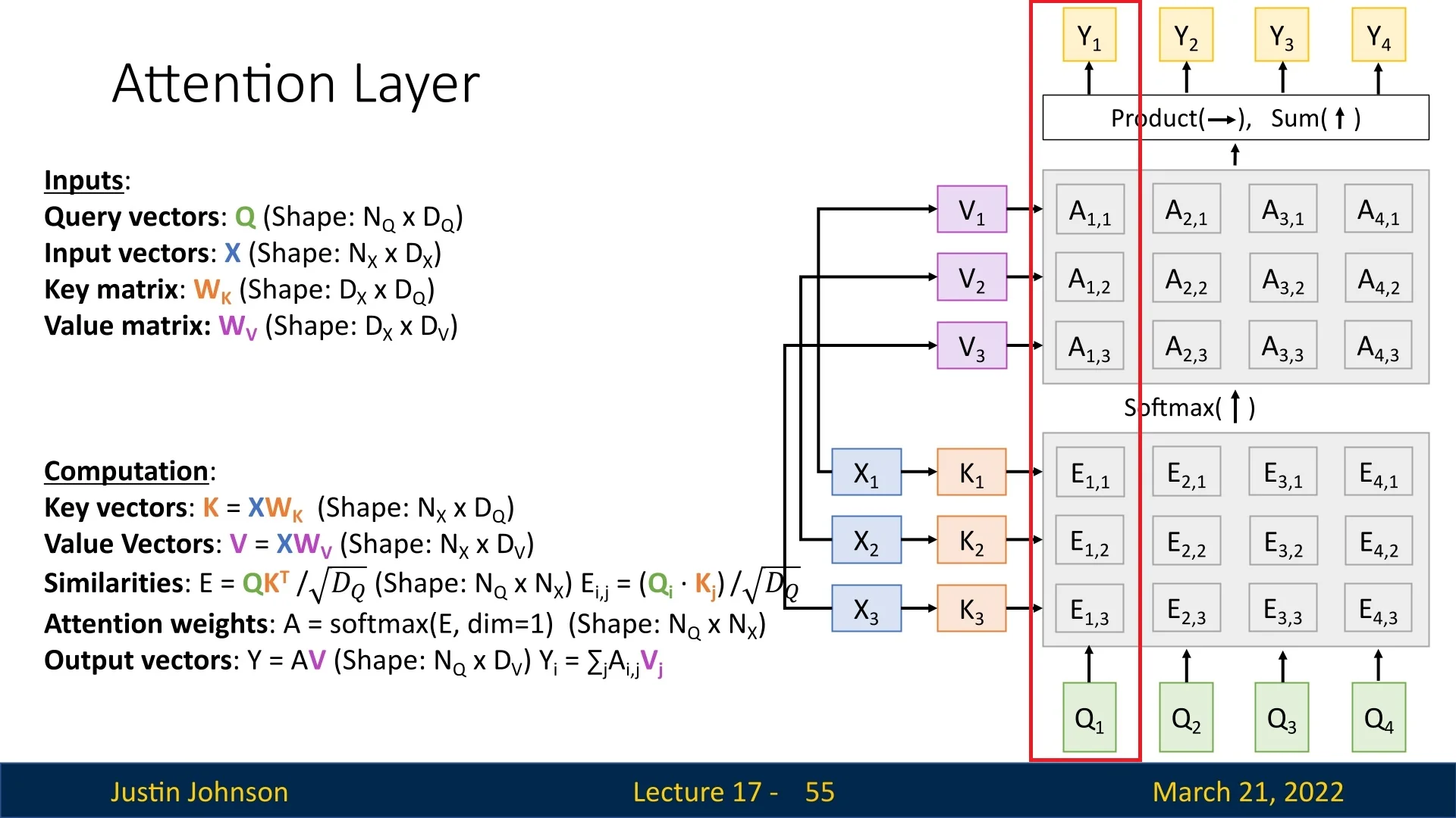
In Figure 17.10, the red-boxed column highlights the computations associated with the query vector \(\textcolor [rgb]{0.471,0.694,0.318}{Q_1}\). The process follows these steps:
- 1.
- Generating Key and Value Vectors: The input vectors \(\textcolor [rgb]{0.267,0.447,0.769}{X} = \{\textcolor [rgb]{0.267,0.447,0.769}{X_1}, \textcolor [rgb]{0.267,0.447,0.769}{X_2}, \textcolor [rgb]{0.267,0.447,0.769}{X_3}\}\) are transformed into key and value vectors using learnable projection matrices: \begin {equation} \textcolor [rgb]{0.929,0.502,0.212}{K} = \textcolor [rgb]{0.267,0.447,0.769}{X} \textcolor [rgb]{0.929,0.502,0.212}{W_K}, \quad \textcolor [rgb]{0.769,0.369,0.800}{V} = \textcolor [rgb]{0.267,0.447,0.769}{X} \textcolor [rgb]{0.769,0.369,0.800}{W_V}. \end {equation} This results in \(\textcolor [rgb]{0.929,0.502,0.212}{K} = \{\textcolor [rgb]{0.929,0.502,0.212}{K_1}, \textcolor [rgb]{0.929,0.502,0.212}{K_2}, \textcolor [rgb]{0.929,0.502,0.212}{K_3}\}\) and \(\textcolor [rgb]{0.769,0.369,0.800}{V} = \{\textcolor [rgb]{0.769,0.369,0.800}{V_1}, \textcolor [rgb]{0.769,0.369,0.800}{V_2}, \textcolor [rgb]{0.769,0.369,0.800}{V_3}\}\).
- 2.
- Computing Similarity Scores: The query vector \(\textcolor [rgb]{0.471,0.694,0.318}{Q_1}\) is compared against all key vectors \(\textcolor [rgb]{0.929,0.502,0.212}{K}\) using the scaled dot product, yielding the corresponding column of \(\textcolor [rgb]{0.236,0.236,0.236}{E^T}\), containing unnormalized alignment scores: \begin {equation} [\textcolor [rgb]{0.236,0.236,0.236}{E_{1,1}}, \textcolor [rgb]{0.236,0.236,0.236}{E_{1,2}}, \textcolor [rgb]{0.236,0.236,0.236}{E_{1,3}}]^T. \end {equation} Each \(\textcolor [rgb]{0.236,0.236,0.236}{E_{1,j}}\) represents the similarity between \(\textcolor [rgb]{0.471,0.694,0.318}{Q_1}\) and key \(\textcolor [rgb]{0.929,0.502,0.212}{K_j}\).
- 3.
- Normalizing Attention Weights: Applying the softmax function converts these scores into a probability distribution over the keys: \begin {equation} [\textcolor [rgb]{0.236,0.236,0.236}{A_{1,1}}, \textcolor [rgb]{0.236,0.236,0.236}{A_{1,2}}, \textcolor [rgb]{0.236,0.236,0.236}{A_{1,3}}]^T. \end {equation}
- 4.
- Computing the Output Vector: The final output \(\textcolor [rgb]{1.0,0.816,0.267}{Y_1}\) is obtained as a weighted sum of the value vectors \(\textcolor [rgb]{0.769,0.369,0.800}{V}\) using the attention weights: \begin {equation} \textcolor [rgb]{1.0,0.816,0.267}{Y_1} = \textcolor [rgb]{0.236,0.236,0.236}{A_{1,1}} \textcolor [rgb]{0.769,0.369,0.800}{V_1} + \textcolor [rgb]{0.236,0.236,0.236}{A_{1,2}} \textcolor [rgb]{0.769,0.369,0.800}{V_2} + \textcolor [rgb]{0.236,0.236,0.236}{A_{1,3}} \textcolor [rgb]{0.769,0.369,0.800}{V_3}, \quad \textcolor [rgb]{1.0,0.816,0.267}{Y_1} \in \mathbb {R}^{D_V}. \end {equation}
This structured visualization clarifies the relationship between \(\textcolor [rgb]{0.471,0.694,0.318}{Q}\), \(\textcolor [rgb]{0.929,0.502,0.212}{K}\), and \(\textcolor [rgb]{0.769,0.369,0.800}{V}\), reinforcing how attention dynamically selects relevant information. The same process is applied to each query vector and set of input vectors to produce the rest of the outputs: \(\textcolor [rgb]{1.0,0.816,0.267}{Y} = \{\textcolor [rgb]{1.0,0.816,0.267}{Y_1}, ..., \textcolor [rgb]{1.0,0.816,0.267}{Y_{N_Q}}\}.\)
17.4.6 Towards Self-Attention
The Attention Layer provides a flexible mechanism to focus on the most relevant information in a given input. However, in previous sections, the queries \(\textcolor [rgb]{0.471,0.694,0.318}{Q}\) and inputs \(\textcolor [rgb]{0.267,0.447,0.769}{X}\) originated from different sources.
A particularly powerful case emerges when we apply attention within the same sequence, allowing each element to attend to all others, including itself. This special configuration is known as Self-Attention, where queries, keys, and values are all derived from the same input sequence:
\[ \textcolor [rgb]{0.471,0.694,0.318}{Q} = \textcolor [rgb]{0.267,0.447,0.769}{X} \textcolor [rgb]{0.471,0.694,0.318}{W_Q}, \quad \textcolor [rgb]{0.929,0.502,0.212}{K} = \textcolor [rgb]{0.267,0.447,0.769}{X} \textcolor [rgb]{0.929,0.502,0.212}{W_K}, \quad \textcolor [rgb]{0.769,0.369,0.800}{V} = \textcolor [rgb]{0.267,0.447,0.769}{X} \textcolor [rgb]{0.769,0.369,0.800}{W_V}. \]
This transformation enables each element in the sequence to selectively aggregate information from all others, facilitating a global receptive field. Unlike recurrence-based models, self-attention allows relationships between distant elements to be captured efficiently while supporting highly parallelized computation.
The ability of self-attention to process entire sequences in parallel has made it foundational to modern architectures such as the Transformer [664]. In the next section, we formally define self-attention mathematically, detailing its computation and role in deep learning architectures.
17.5 Self-Attention
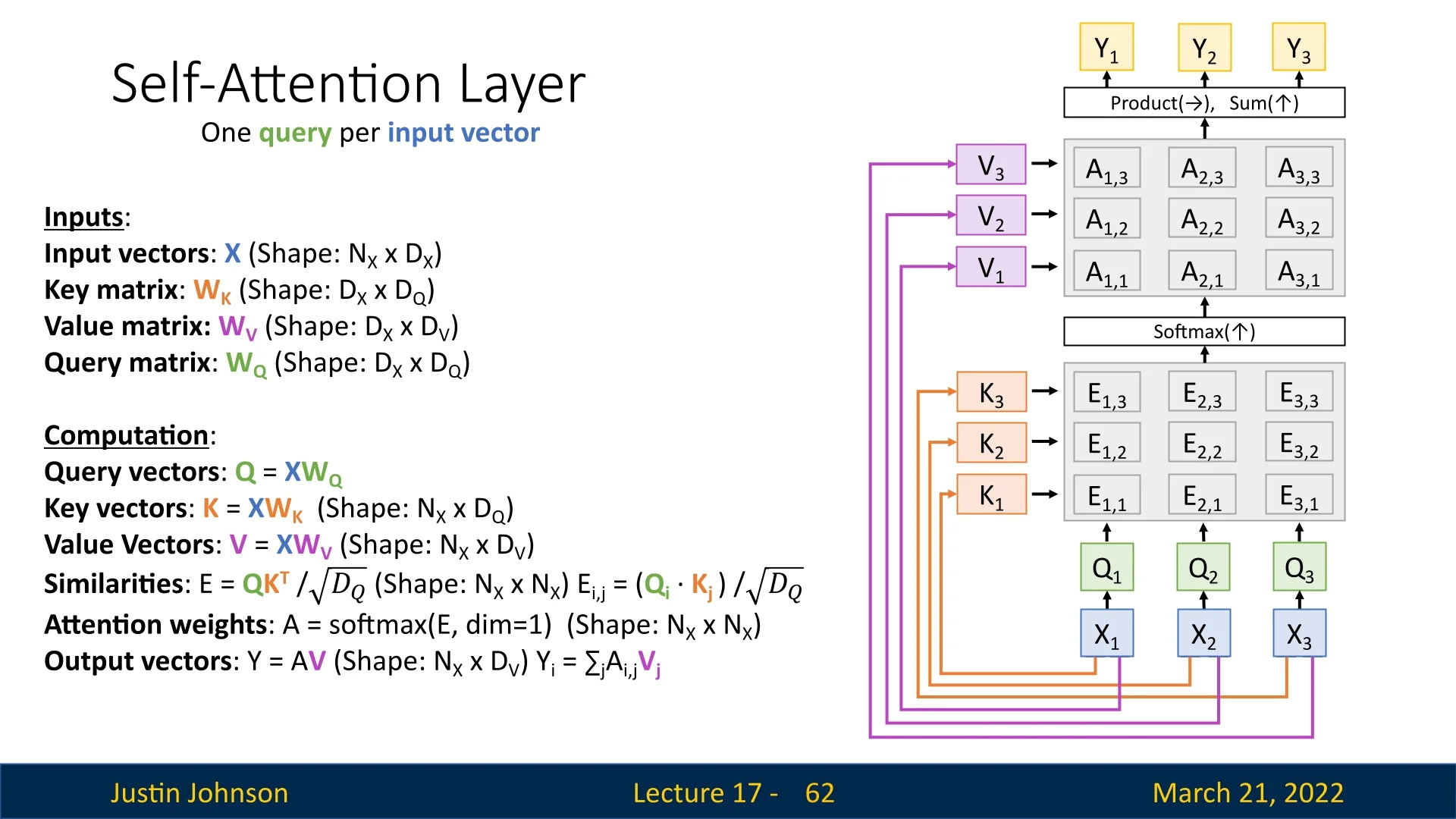
The Self-Attention Layer extends the attention mechanism by enabling each element in an input sequence to compare itself with every element in the sequence. Unlike the Attention Layer described in subsection 17.4.5, where queries and inputs could originate from different sources, self-attention generates its queries, keys, and values from the same input set.
This formulation retains the same structure as the regular attention layer, with one key modification: instead of externally provided query vectors, we now predict them using a learnable transformation \( \textcolor [rgb]{0.471,0.694,0.318}{W_Q} \). The rest of the computations—including key and value transformations, similarity computations, and weighted summation—remain unchanged.
17.5.1 Mathematical Formulation of Self-Attention
Given an input set of vectors \( \textcolor [rgb]{0.267,0.447,0.769}{X} = \{\textcolor [rgb]{0.267,0.447,0.769}{X_1}, \dots , \textcolor [rgb]{0.267,0.447,0.769}{X_{N_X}}\} \), self-attention computes:
- Query Vectors: \( \textcolor [rgb]{0.471,0.694,0.318}{Q} = \textcolor [rgb]{0.267,0.447,0.769}{X} \textcolor [rgb]{0.471,0.694,0.318}{W_Q} \)
- Key Vectors: \( \textcolor [rgb]{0.929,0.502,0.212}{K} = \textcolor [rgb]{0.267,0.447,0.769}{X} \textcolor [rgb]{0.929,0.502,0.212}{W_K} \)
- Value Vectors: \( \textcolor [rgb]{0.769,0.369,0.800}{V} = \textcolor [rgb]{0.267,0.447,0.769}{X} \textcolor [rgb]{0.769,0.369,0.800}{W_V} \)
The computations proceed as follows:
\begin {equation} \textcolor [rgb]{0.236,0.236,0.236}{E} = \frac {\textcolor [rgb]{0.471,0.694,0.318}{Q} \textcolor [rgb]{0.929,0.502,0.212}{K^T}}{\sqrt {D_Q}}, \quad \textcolor [rgb]{0.236,0.236,0.236}{A} = \mbox{softmax}(\textcolor [rgb]{0.236,0.236,0.236}{E}, \mbox{dim} = 1), \quad \textcolor [rgb]{1.0,0.816,0.267}{Y} = \textcolor [rgb]{0.236,0.236,0.236}{A} \textcolor [rgb]{0.769,0.369,0.800}{V}. \end {equation}
As before, the output vector for each input \( \textcolor [rgb]{1.0,0.816,0.267}{Y_i} \) is computed as a weighted sum:
\begin {equation} \textcolor [rgb]{1.0,0.816,0.267}{Y_i} = \sum _j \textcolor [rgb]{0.236,0.236,0.236}{A_{i,j}} \textcolor [rgb]{0.769,0.369,0.800}{V_j}. \end {equation}
17.5.2 Non-Linearity in Self-Attention
At first glance, self-attention might appear to be a mostly linear mechanism—performing dot products between \(\mathbf {Q}\) and \(\mathbf {K}\), then using those results to weight \(\mathbf {V}\). However, there is an important source of non-linearity that makes self-attention more expressive than purely linear transformations:
- Softmax Non-Linearity: Once we compute the raw attention scores \(\mathbf {E} = \mathbf {Q}\mathbf {K}^\top / \sqrt {D_Q}\), we normalize each row (per-query) using a softmax: \[ \mathbf {A} = \mathrm {softmax}(\mathbf {E}, \mbox{dim} = 1). \] This softmax operation is an explicit non-linear function [664], ensuring adaptive weighting of each key-value pair and preventing the raw dot products from dominating the final distribution. Unlike purely linear layers that weigh inputs in a fixed manner, softmax-based weighting can concentrate or diffuse attention in a data-dependent way.
- Context-Dependent Weighting: In convolution, filters are fixed spatial kernels that move over the input. In contrast, self-attention dynamically alters how each token (or feature element) attends to every other element [22, 664]. The weighting depends on both the query vector \(\mathbf {Q}\) and the key vectors \(\mathbf {K}\), reflecting learned interactions. This “context dependence” is another key source of non-linearity because the softmax weighting is not a simple linear map but a function of pairwise similarities.
Hence, while self-attention does not apply an explicit activation function (like ReLU) within the dot product, the softmax normalization and token-by-token dynamic weighting create a highly flexible, non-linear transformation of the input \(\mathbf {V}\). In practice, self-attention layers are often combined with additional feedforward networks (including ReLU-like activations) in architectures such as the Transformer [664], further increasing their representational power.
17.5.3 Permutation Equivariance in Self-Attention
Self-attention is inherently permutation equivariant, meaning that permuting the input sequence results in the outputs being permuted in the same way. Formally, let:
- \( f \) be the self-attention function mapping inputs to outputs.
- \( s \) be a permutation function reordering the input sequence.
The property is expressed as:
\begin {equation} f(s(\textcolor [rgb]{0.267,0.447,0.769}{X})) = s(f(\textcolor [rgb]{0.267,0.447,0.769}{X})). \end {equation}
This means that permuting the inputs and then applying self-attention yields the same result as applying self-attention first and then permuting the outputs.
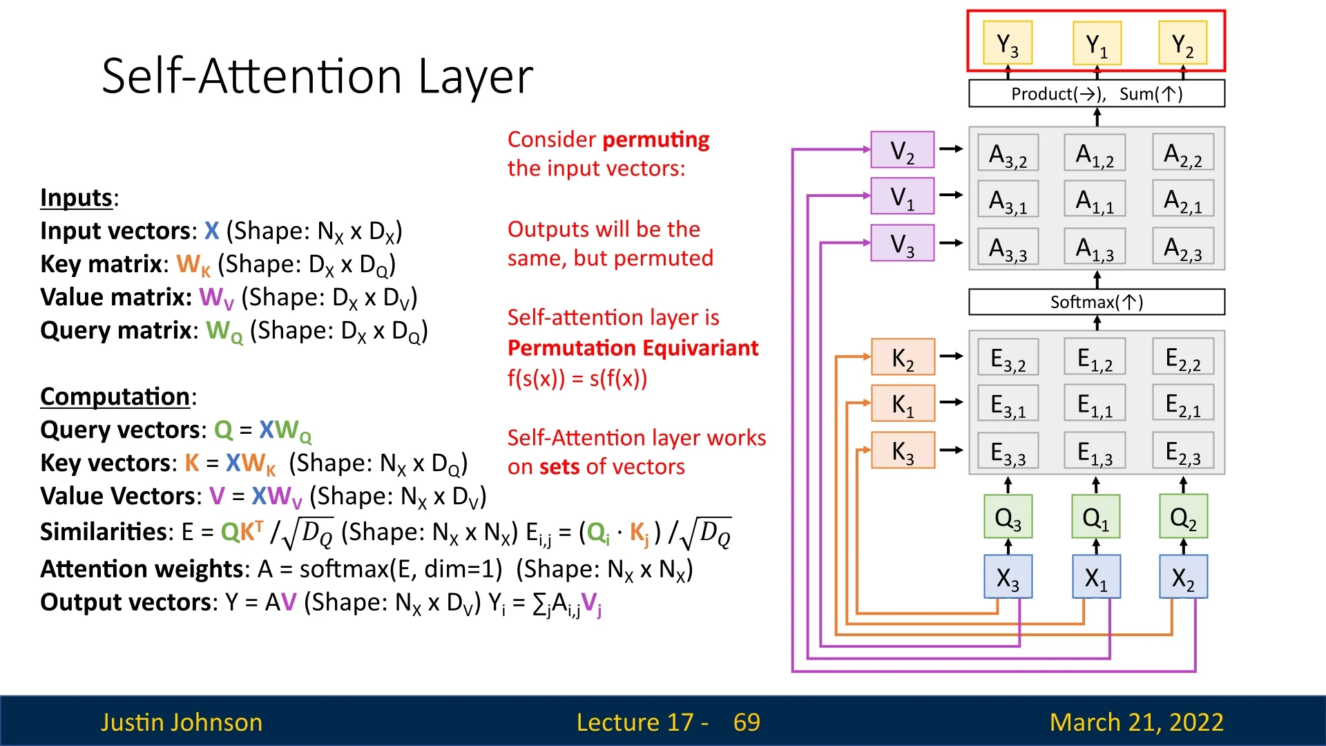
For instance, in Figure 17.12, permuting the input sequence from \(\{X_1, X_2, X_3\}\) to \(\{X_3, X_2, X_1\}\) results in the outputs being permuted to \(\{Y_3, Y_2, Y_1\}\).
When is Permutation Equivariance a Problem?
While permutation equivariance is desirable in tasks that operate on unordered sets (e.g., point cloud processing, certain graph-based tasks), it poses challenges in tasks where sequence order is essential:
- Natural Language Processing (NLP): Word order carries critical meaning. The sentence ”The cat chased the mouse” conveys a different meaning than ”The mouse chased the cat.” A purely permutation-equivariant model would fail to differentiate these cases.
- Image Captioning: The order in which words are generated is crucial. If self-attention does not respect positional information, a model could struggle to generate coherent descriptions.
- Time-Series Analysis: Sequential dependencies (e.g., stock market trends, weather forecasting) require an understanding of past-to-future relationships, which are lost if order is ignored.
To address this, we introduce positional encodings, which explicitly encode sequence order into self-attention models, ensuring that position-dependent tasks retain meaningful structure. Hence, we’ll now explore how positional encodings are designed and integrated into self-attention mechanisms.
17.5.4 Positional Encodings: Introduction
Self-Attention layers, unlike RNNs, do not have an inherent sense of sequence order since they process all tokens in parallel. To incorporate positional information, positional encodings are added to input embeddings before passing them into the model. Two common approaches exist: fixed sinusoidal positional encodings and learnable positional embeddings. Below, we examine the key differences and motivations for using each approach.
Why Not Use Simple Positional Indices?
- Simple Positional Indexing. \begin {equation} \label {eq:simple_index} P_t = t, \quad t \in [1, N], \end {equation} where \( N \) is the sequence length.
-
Drawbacks of Simple Indexing.
- Numerical Instability. Large positional indices may lead to gradient explosion or saturation in deep networks, and can dominate the scale of content embeddings.
- Poor Generalization. If training sequences are shorter than test sequences, the model may fail to generalize to unseen positions.
- Lack of Relative Positioning. Absolute indexing requires the model to learn how index differences influence attention from scratch. The model does not inherently recognize distance relationships, making it inefficient for learning locality-sensitive patterns.
- Normalized Positional Indexing.
As an alternative to simple positional indices, one could normalize indices to a fixed range. This approach keeps positional values bounded: \begin {equation} \label {eq:normalized_index} P_t = \frac {t}{N-1}, \quad t \in [0, N-1]. \end {equation} -
Drawbacks of Normalized Indexing.
- Inconsistency Across Lengths. The same absolute position \(t\) will map to different normalized values depending on \(N\). Consequently, a model cannot associate a stable representation with “token 10” across inputs of varying length.
-
Variable Relative Distances (The “Rubber Band” Effect). Normalization also distorts relative geometry. The normalized distance between adjacent positions is \begin {equation} \label {eq:normalized_step} P_{t+1} - P_t = \frac {1}{N-1}. \end {equation} Thus, the meaning of “one step forward” depends on the total sequence length. For example:
- If \(N=4\), then \(P_t = [0, \tfrac {1}{3}, \tfrac {2}{3}, 1]\), so adjacent tokens differ by \(\tfrac {1}{3}\).
- If \(N=10\), then \(P_t = [0, \tfrac {1}{9}, \tfrac {2}{9}, \dots , 1]\), so adjacent tokens differ by \(\tfrac {1}{9}\).
In other words, the positional space is stretched or compressed as \(N\) changes. This forces the attention mechanism to relearn what “local” means for each length, complicating the learning of reusable patterns such as “attend strongly to the immediate neighbor” or “favor a fixed offset of \(k\) tokens”.
These issues motivate a more principled positional scheme whose functional form is independent of \(N\) and whose structure makes relative offsets easier to recover. This intuition leads naturally to the sinusoidal positional encodings introduced in the original Transformer, which are bounded, length-agnostic, and designed so that fixed offsets correspond to predictable transformations in the encoding space.
17.5.5 Sinusoidal Positional Encoding
When Vaswani et al. introduced the Transformer, they faced a fundamental structural limitation of self-attention: without recurrence or convolution, the layer has no built-in notion of token order. A sentence such as “The dog bit the man” contains the same set of tokens as “The man bit the dog”, yet the meaning changes because the order changes. Hence, the model must be given an explicit and systematic notion of position.
The original solution is sinusoidal positional encoding, a fixed, parameter-free function that maps each position index \(t\) to a vector \(\mathbf {p}_t \in \mathbb {R}^{d}\). This vector is added to the content embedding before the first attention layer: \begin {equation} \label {eq:chapter17_pe_addition} \mathbf {x}'_t = \mathbf {x}_t + \mathbf {p}_t, \end {equation} so that every subsequent layer can condition jointly on what the token is and where it appears.
Mathematical Definition and Frequency Bands
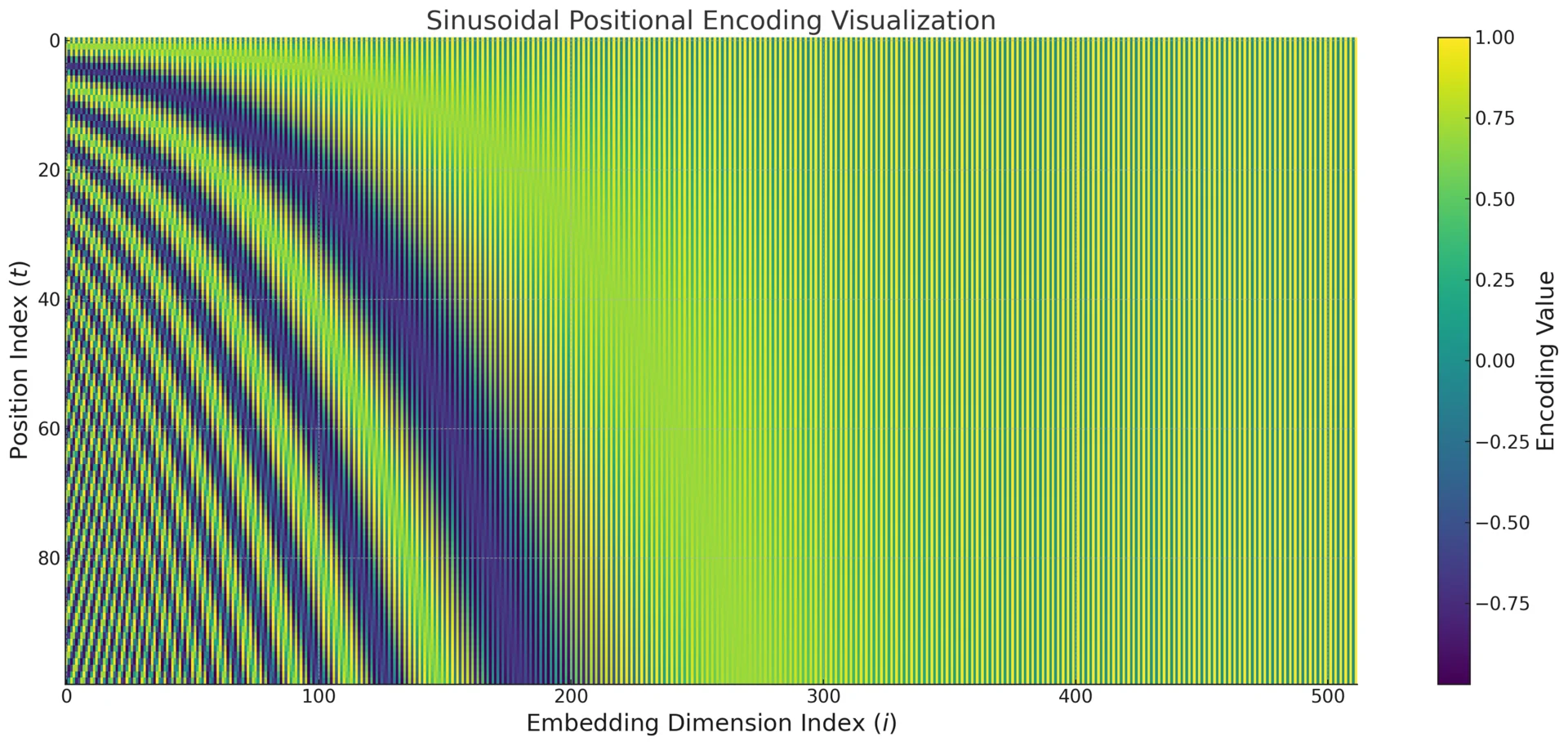
Let \(d\) denote the embedding dimension (and the positional encoding dimension), typically matching the model width (e.g., \(d=512\) in the original Transformer). The sinusoidal encoding partitions the \(d\) coordinates into \(\frac {d}{2}\) frequency bands. Each band contributes exactly two dimensions: one sine and one cosine component at the same angular frequency. This pairing is why \(d\) is chosen to be even in practice.
For each band index \(k \in \{0,1,\dots ,\frac {d}{2}-1\}\), define: \begin {equation} \label {eq:chapter17_sinusoidal_encoding} \begin {aligned} \mathbf {p}_t(2k) &= \sin (\omega _k t),\\ \mathbf {p}_t(2k+1) &= \cos (\omega _k t), \end {aligned} \qquad \omega _k = \frac {1}{10000^{\frac {2k}{d}}}. \end {equation}
Equivalently, for a dimension index \(i \in \{0,1,\dots ,d-1\}\), the definition pairs sine and cosine in adjacent dimensions by setting \(i=2k\) and \(i=2k+1\). The key symbols are:
- \(\displaystyle t\): the absolute position index within the sequence (e.g., \(0,1,2,\dots \)).
- \(\displaystyle d\): the encoding dimension, equal to the token embedding dimension.
- \(\displaystyle k\): the frequency-band index that groups each \(\sin \)–\(\cos \) pair.
- \(\displaystyle \omega _k\): the angular frequency assigned to band \(k\).
The band index \(k\) therefore controls how quickly the corresponding two coordinates change with \(t\). Small \(k\) yields large \(\omega _k\) (rapid oscillations), while large \(k\) yields small \(\omega _k\) (slow oscillations). Stacking \(\frac {d}{2}\) such bands gives a single vector \(\mathbf {p}_t\) that can represent both fine-grained and coarse positional structure simultaneously.
Intuition: A Multi-Scale, Continuous Counter
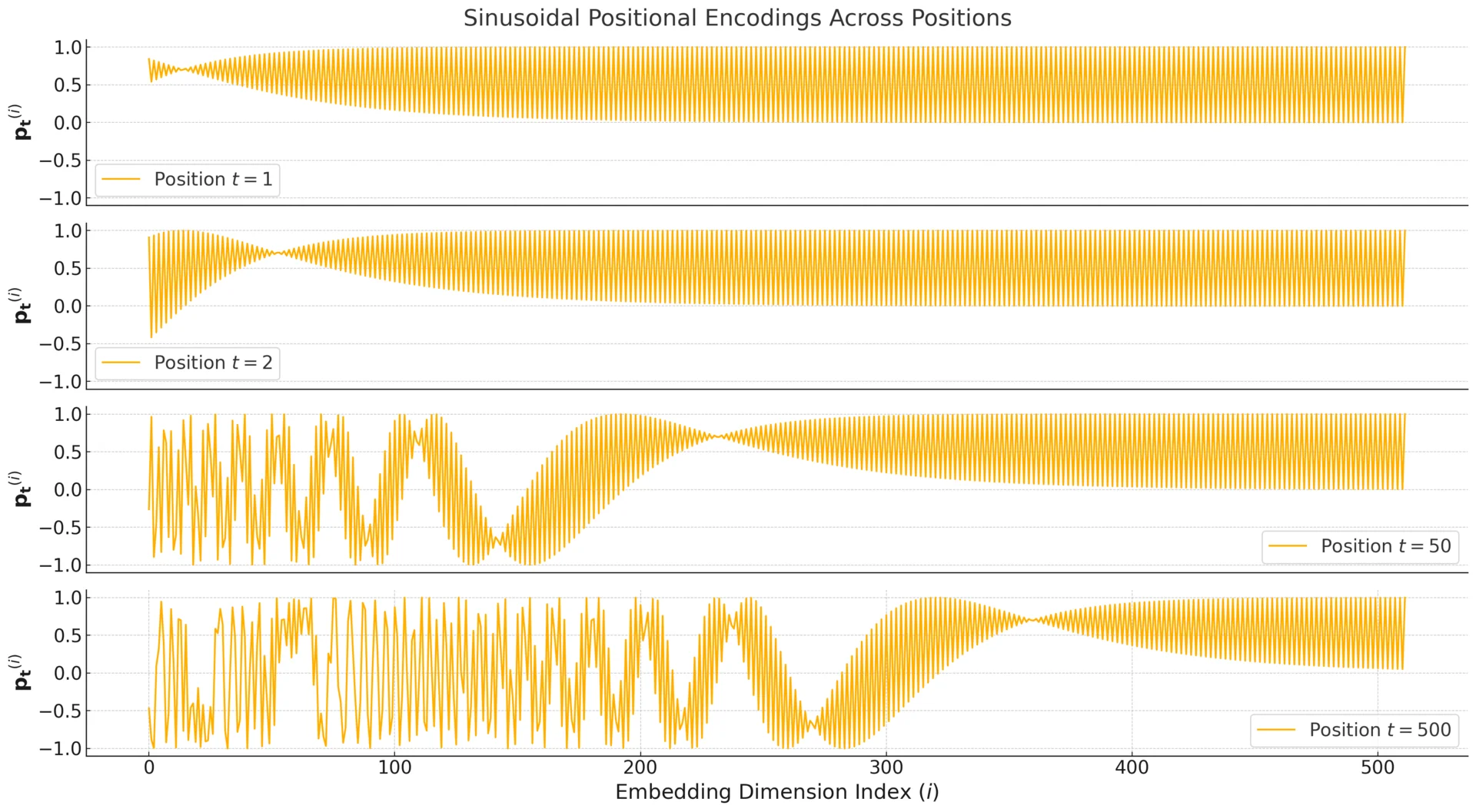
A helpful way to interpret sinusoidal positional encoding is to treat it as a multi-scale representation of the integer index \(t\). Instead of describing position with a single scalar (such as \(t\) or a normalized \(\tfrac {t}{N}\)), the Transformer assigns each position a vector \(\mathbf {p}_t \in \mathbb {R}^d\) that combines \(\tfrac {d}{2}\) frequency bands. Each band \(k\) contributes a two-dimensional coordinate that records the phase of \(\omega _k t\): \[ \mathbf {b}^{(k)}_t = \begin {bmatrix} \sin (\omega _k t)\\ \cos (\omega _k t) \end {bmatrix}, \qquad \mathbf {p}_t = \bigl [ \mathbf {b}^{(0)}_t \; \mathbf {b}^{(1)}_t \; \cdots \; \mathbf {b}^{(\frac {d}{2}-1)}_t \bigr ]. \] Thus, \(\mathbf {p}_t\) can be viewed as a snapshot of many “position sensors” operating at different temporal resolutions.
This resembles the behavior of a binary counter: low-order bits change frequently, whereas high-order bits change slowly and encode coarse location. Here, the discrete flips are replaced by smooth oscillations. The key advantage over naive indexing is scale coverage: \(\mathbf {p}_t\) does not compress position into a single number whose meaning depends on sequence length. Instead, it distributes positional information across many frequencies, so the model can reliably detect both small and large positional changes.
This structure supplies two complementary signals:
- Local sensitivity. High-frequency bands (small \(k\)) respond strongly to \(t \rightarrow t+1\), so adjacent tokens receive clearly different positional vectors. This makes short-range order patterns easy to learn.
- Global context. Low-frequency bands (large \(k\)) change slowly, so they separate far-apart positions even when high-frequency bands have already cycled through many periods. This helps the model distinguish broad regions of a long sequence.
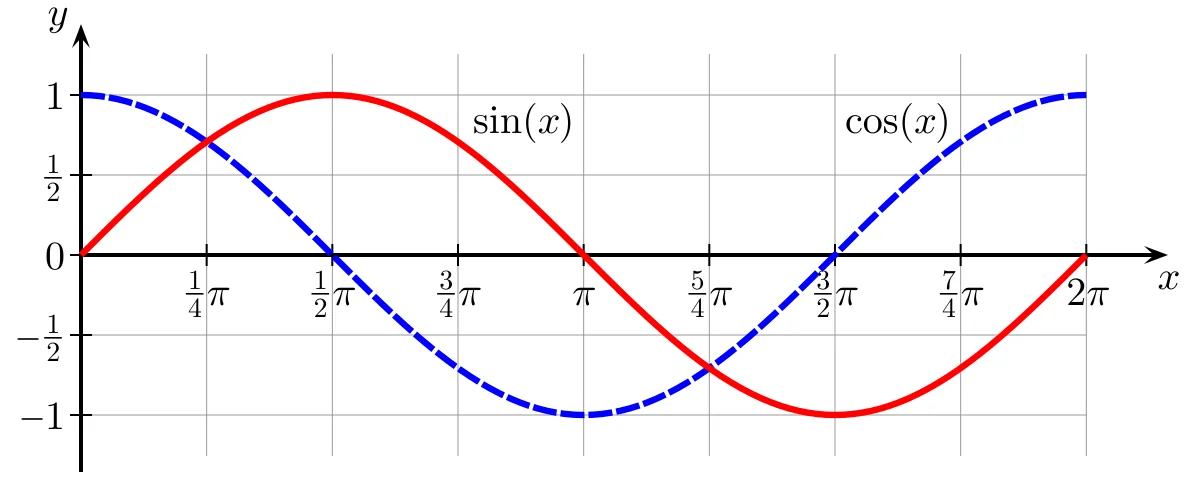
Why Sine and Cosine Pairs?
A single sinusoid is periodic and therefore ambiguous when used alone. For instance, \(\sin (\pi /6)=\sin (5\pi /6)\), so two distinct angles can share the same sine value. By pairing \(\sin (\omega _k t)\) with \(\cos (\omega _k t)\), each band \(k\) becomes a point on the unit circle that specifies the phase of \(\omega _k t\) in two dimensions: \[ \mathbf {b}^{(k)}_t = \bigl (\sin (\omega _k t), \cos (\omega _k t)\bigr ). \] Even if two positions produce similar sine values for a given band, their cosine values typically differ. Across \(\tfrac {d}{2}\) bands, the concatenated vector \(\mathbf {p}_t\) becomes a high-dimensional positional signature without requiring learned parameters.
Why the Base \(10000\)? Wavelength Coverage
The constant \(10000\) controls the range of frequencies and thus the positional “resolutions” available to the model. Because the exponent \(\frac {2k}{d}\) grows linearly with \(k\), the frequencies \(\omega _k\) decrease exponentially. This yields a geometric progression of wavelengths. For band \(k\), the wavelength is: \begin {equation} \label {eq:chapter17_wavelength} \lambda _k = \frac {2\pi }{\omega _k} = 2\pi \cdot 10000^{\frac {2k}{d}}. \end {equation}
This construction ensures that the encoding contains:
- Very short wavelengths in early bands, which sharply separate adjacent positions.
- Very long wavelengths in late bands, which change meaningfully only across large distances.
In typical settings (e.g., \(d=512\)), this spans a wide but numerically stable spectrum of positional scales while keeping all coordinates bounded in \([-1,1]\).
Concrete Frequency Micro-Example For a toy dimension \(d=8\), the four frequency bands are: \[ \omega _0 = 1, \quad \omega _1 = 10000^{-0.25} = \frac {1}{10}, \quad \omega _2 = 10000^{-0.5} = \frac {1}{100}, \quad \omega _3 = 10000^{-0.75} = \frac {1}{1000}. \] The first pair thus changes rapidly with \(t\), while the last pair changes very slowly, illustrating how the construction allocates both fine and coarse positional resolution.
Frequency Variation and Intuition
A clearer way to interpret the frequency sweep is to view each band as a positional sensor defined by a distinct angular frequency \(\omega _k\). For small \(k\), \(\omega _k\) is large and the band is highly sensitive to single-step changes. For large \(k\), \(\omega _k\) is small and the band changes slowly, so it provides stable separation over long distances.
This layered design prevents two complementary failure modes:
- If only slow bands existed, \(\mathbf {p}_t\) and \(\mathbf {p}_{t+1}\) would be nearly identical, weakening the model’s ability to detect fine-grained order.
- If only fast bands existed, the positional patterns would repeat frequently, and far-apart positions could become difficult to distinguish reliably.
The geometric spacing of \(\omega _k\) is therefore essential: it distributes sensitivity smoothly across scales. As a result, the full vector \(\mathbf {p}_t\) retains information about both small offsets (e.g., neighbor relations, short phrases) and large offsets (e.g., clause-level or document-level structure), which aligns with the range of dependencies that attention must model.
Concrete Example: “I Can Buy Myself Flowers”
To make the multi-scale behavior tangible, consider a simplified case with \(d=4\), which yields two bands: a high-frequency pair with \(\omega _0=1\) and a low-frequency pair with \[ \omega _1=\frac {1}{10000^{2/4}}=\frac {1}{100}=0.01. \] Their wavelengths differ sharply: \[ \lambda _0 = 2\pi \approx 6.28, \qquad \lambda _1 = \frac {2\pi }{0.01} = 200\pi \approx 628. \] Thus, Band 0 completes a full cycle every few tokens, while Band 1 changes perceptibly only over hundreds of tokens.
Concretely, the positional vector is \[ \mathbf {p}_t = \bigl [ \sin (t), \cos (t), \sin (0.01t), \cos (0.01t) \bigr ]. \] For early positions, the first pair provides strong local separation: moving from \(t=0\) to \(t=1\) produces a large, easily detectable change. The second pair provides a slow baseline: it changes very little across \(t=0,1,2\), but would meaningfully differentiate positions that are hundreds of tokens apart.
| Token | Pos (\(t\)) | Band 0 (\(\omega _0=1\)) | Band 1 (\(\omega _1=0.01\))
| ||
|---|---|---|---|---|---|
| \(\sin (t)\) | \(\cos (t)\) | \(\sin (0.01t)\) | \(\cos (0.01t)\) | ||
| I | 0 | \(0\) | \(1\) | \(0\) | \(1\) |
| Can | 1 | \(\approx 0.84\) | \(\approx 0.54\) | \(\approx 0.01\) | \(\approx 1.00\) |
| Buy | 2 | \(\approx 0.91\) | \(\approx -0.42\) | \(\approx 0.02\) | \(\approx 1.00\) |
This toy case mirrors the full design: a real Transformer allocates many more bands, so that this fast-to-slow coverage becomes dense across the embedding space. The resulting \(\mathbf {p}_t\) is therefore not a single-scale counter, but a multi-scale positional fingerprint.
How Relative Position Awareness Emerges
The value of sinusoidal encoding is not only that it labels absolute positions, but also that it makes relative distance visible to attention computations in a systematic way. This can be seen by examining a single band \(k\). Define the 2D band vector: \[ \mathbf {b}_t^{(k)} = \begin {bmatrix} \sin (\omega _k t)\\ \cos (\omega _k t) \end {bmatrix}. \] Using trigonometric identities, the inner product between two positions separated by an offset \(o\) satisfies: \begin {equation} \label {eq:chapter17_band_inner_product} \left (\mathbf {b}_t^{(k)}\right )^\top \mathbf {b}_{t+o}^{(k)} = \cos (\omega _k o). \end {equation}
Crucially, \(\cos (\omega _k o)\) depends only on the offset \(o\), not on the absolute position \(t\). Thus, within each band, the similarity of two positional codes is a direct, frequency-specific function of distance. Short offsets and long offsets produce different similarity signatures.
Because the full positional vector \(\mathbf {p}_t\) concatenates \(\frac {d}{2}\) such bands, the aggregate positional similarity becomes a multi-scale signature of distance: \[ \mathbf {p}_t^\top \mathbf {p}_{t+o} = \sum _{k=0}^{\frac {d}{2}-1} \cos (\omega _k o). \] Self-attention relies on dot products between linearly projected token representations. After \(\mathbf {p}_t\) is added to content embeddings, these dot-product comparisons can naturally incorporate this structured distance signal. As a result, the model can learn attention patterns that respond differently to short-range and long-range offsets using the same positional construction, without depending on a separate learned table of relative positions.
Does Positional Information Vanish in Deeper Layers?
One might worry that adding positional information only at the input could cause it to be diluted in deep models. In practice, Transformer design choices mitigate this concern:
- Residual connections. These preserve positional and content cues across layers.
- Layer normalization. This maintains stable signal scales and training dynamics, keeping positional information usable throughout depth.
Why Sinusoidal Encoding Addresses Simpler Schemes
Compared with naive approaches such as raw indices or single-scale normalizations, sinusoidal encodings provide:
- Multi-scale coverage. Different frequencies simultaneously support local order resolution and long-range separation.
- A consistent distance signal. Within each frequency band, similarity depends directly on the relative offset.
- Parameter-free generality. The encoding is fixed, stable, and defined for arbitrary \(t\), enabling principled use on longer sequences.
Conclusion on Sinusoidal Positional Encoding
Sinusoidal positional encoding is an effective, parameter-free solution to the permutation-insensitivity of self-attention. Its carefully spaced frequency bands provide a single representation that preserves information about both small and large positional differences, and the resulting dot-product structure makes relative distance naturally visible to attention computations. However, because the geometry is fixed, it cannot adapt to dataset-specific structure. We therefore next consider learnable positional embeddings, which trade this fixed formulation for increased flexibility.
17.5.6 Learned Positional Encodings: An Alternative Approach
While sinusoidal encodings provide a fixed and mathematically structured scheme, another widely used strategy is to learn positional representations directly from data. In this approach, position is not generated by a function \(f(t)\). Instead, the model allocates a separate trainable vector to each absolute index up to a predefined maximum length. Concretely, every position \( t \in \{0,\dots ,N_{\max }-1\} \) is assigned a learnable embedding \( \mathbf {P}_t \in \mathbb {R}^d \), which is added to the token embedding before the first self-attention block. This section explains the mechanism, motivates when learned absolute encodings are a natural fit, and highlights their core limitations relative to sinusoidal encodings.
Definition and Mechanics: A Trainable Embedding Matrix Implementation-wise, learned absolute positional encodings are realized as a parameter matrix \( \mathbf {P} \in \mathbb {R}^{N_{\max }\times d} \), analogous to the token embedding matrix. Calling this structure a “lookup table” is accurate in the engineering sense: at inference time, the model simply selects the row corresponding to index \(t\). Formally, \[ \mathbf {P}_t = \mathbf {P}[t], \qquad \mathbf {P}_t \in \mathbb {R}^d. \] These vectors are initialized randomly and updated via backpropagation alongside all other Transformer parameters. The input representation at position \(t\) becomes \[ \mathbf {x}'_t = \mathbf {x}_t + \mathbf {P}_t, \] so the network can learn how much and in what direction each absolute index should bias the content embedding. If the task repeatedly rewards a distinctive behavior at a specific index, gradients can directly sculpt \(\mathbf {P}_t\) into a strong positional marker for that role.
What This Design Assumes Learned absolute embeddings implicitly assume a known or stable maximum length \(N_{\max }\). Unlike sinusoids, which define \(\mathbf {p}_t\) for all integers \(t\), the learned scheme only stores parameters for indices \(0\) through \(N_{\max }-1\). Thus, the representation is flexible within the trained window, but not inherently designed for arbitrary-length extrapolation.
Examples of Learned Absolute Positional Encodings
- BERT (Bidirectional Encoder Representations from Transformers) [121]: BERT uses learned absolute positional embeddings within a fixed maximum length. This choice aligns with the model’s emphasis on sentence- and segment-level structure, where certain absolute locations, boundary-adjacent tokens, and special markers (e.g., [CLS] and [SEP]) are consistently meaningful. A learned table can assign these frequently used indices distinctive vectors that are directly optimized for the downstream objectives.
- GPT (Generative Pre-trained Transformer) [511]: Early GPT models also adopt learned absolute positional embeddings for causal sequence modeling, allowing the model to tune position-specific vectors for next-token prediction within a fixed context window. This is especially natural when training and inference contexts are closely matched.
- Vision Transformers (ViT) [134]: ViT uses learned positional embeddings for sequences of image patches. Here the “sequence” is derived from a (roughly) fixed spatial grid of patches, so learning a distinct embedding per patch index can help the model capture dataset-specific regularities about spatial layout. In practice, when transferring across image resolutions, these embeddings are commonly resized by interpolation, which preserves a useful initialization but also underscores that the method is tied to an assumed maximum grid size.
Notably, some later designs replace learned absolute embeddings with explicitly relative mechanisms. For example, T5 uses relative position biases rather than input-added learned absolute vectors [517]. We discuss such relative schemes separately when comparing absolute and relative approaches.
Where Learned Embeddings Can Be Especially Useful? Learned absolute embeddings tend to be most attractive when two conditions hold: the domain has a stable maximum length and the data exhibits index-specific conventions. Several examples illustrate this pattern:
- Fixed-format text and documents. In structured templates, forms, or code-like formats, particular indices can reliably mark headers, separators, or standardized fields. A learned table can store a strong, position-specific marker that the model can exploit immediately, rather than requiring deeper layers to amplify a smooth functional signal.
- Patch-based vision. When images are represented as a consistent grid of patches, absolute index can correlate with stable spatial priors introduced by dataset construction (e.g., object-centered crops). Learned embeddings can absorb such priors directly into the position space.
- Well-bounded biological or symbolic sequences. If sequences follow standardized length conventions or contain known anchor regions, learned embeddings can encode these regularities as explicit positional signatures.
Intuition: A “Ruler” Versus a “Trainable Index Map”. A concise way to contrast learned and sinusoidal approaches is the following analogy:
- Sinusoidal encoding resembles a ruler. It provides a smooth, multi-scale coordinate system. Because it is a function of \(t\), it naturally defines encodings beyond the lengths seen during training and imposes a consistent notion of distance-related structure.
- Learned encoding resembles a trainable index map. The model assigns a dedicated vector to each slot and can tune these slots to match the data distribution. If a particular index plays a special role, the model can encode that role directly in \(\mathbf {P}_t\), without requiring downstream layers to “sharpen” a smooth wave into a boundary signal.
Handling Longer Sequences Than Seen in Training A natural concern is how learned absolute embeddings handle sequences longer than the maximum length used to define the table. The strict answer is that they do not generalize automatically: if \(L > N_{\max }\), there is no learned vector \(\mathbf {P}_{L-1}\) to retrieve. Common practical responses include:
- Truncation (common in NLP). Inputs are clipped to \(N_{\max }\), which preserves correctness but discards long-range context.
- Table extension with further training. One can expand \(\mathbf {P}\) to a larger \(N_{\max }\), initialize new rows (often randomly or by copying/interpolating existing patterns), and continue training. This is an engineering fix rather than a principled extrapolation guarantee.
- Interpolation (common in ViT). When changing patch grid size, existing 2D positional embeddings are resized to the new resolution, providing a smooth transfer initialization but not the same kind of length-agnostic behavior offered by functional encodings.
These workarounds underscore the central trade-off: learned absolute encodings are highly adaptable within the trained regime but are weaker for robust length generalization.
Pros & Cons of Learned Positional Embeddings
Pros:
- Adaptable to complex positional semantics. Since each position \(t\) has its own vector \(\mathbf {P}_t\), the model can represent idiosyncratic index-dependent patterns that do not follow a smooth or periodic trend. This is valuable when the data contains sharp, index-specific roles (e.g., template headers, special tokens, or standardized fields).
- Task-specific optimization. The embeddings \(\{\mathbf {P}_0,\dots ,\mathbf {P}_{N_{\max }-1}\}\) are learned jointly with the rest of the model, allowing the network to calibrate how absolute indices shape local and global dependencies in the target domain. This can be a capacity-efficient way to encode “positional special cases,” reducing the need for deeper layers to derive the same emphasis from a fixed functional pattern.
- Empirical gains in some settings. Several studies report that learned absolute embeddings can match or outperform fixed encodings in tasks where sequence lengths are well-bounded and positional conventions are strong [296, 580].
Cons:
- Limited extrapolation to longer sequences. If training and inference lengths exceed \(N_{\max }\), the model has no learned vectors for unseen positions without modifying or extending the table. By contrast, sinusoidal encodings define \(\mathbf {p}_t\) for all integer \(t\).
- Increased parameterization and memory. A unique vector per position yields \(N_{\max }\times d\) additional parameters. This overhead is modest for small windows but grows linearly with context length.
- Reduced structural transparency. Unlike sinusoidal encodings, learned absolute embeddings do not impose a guaranteed functional relationship between distance \(|i-j|\) and positional similarity. Understanding how \(\mathbf {P}_i\) and \(\mathbf {P}_j\) relate typically requires post-hoc analysis, and behavior at rarely observed indices may be less predictable.
Conclusion on Learned Positional Embeddings Learned absolute positional encodings offer a flexible alternative to sinusoidal functions. They are particularly attractive when sequence length is well-bounded and the domain exhibits index-specific structure that benefits from explicit positional markers, as seen in early LLMs and patch-based vision models [121, 511, 134]. However, this flexibility comes with limited extrapolation to longer sequences, additional parameters, and weaker built-in structure across distances. In practice, the choice between fixed sinusoidal encodings and learned absolute embeddings depends on whether the application prioritizes robust length generalization or domain-specific positional specialization [295].
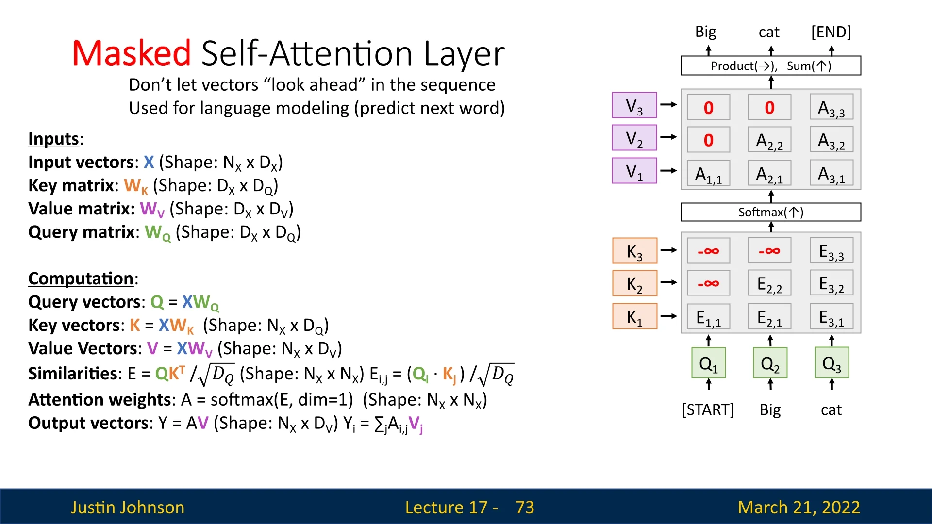
17.5.7 Masked Self-Attention Layer
While standard self-attention allows each token to attend to every other token in the sequence, there are many tasks where we need to enforce a constraint that prevents tokens from ”looking ahead” at future elements. This is particularly important in auto-regressive models, such as language modeling, where each token should be predicted solely based on previous tokens. Without such constraints, the model could trivially learn to predict future tokens by directly attending to them, preventing it from developing meaningful contextual representations.
Why Do We Need Masking?
Consider a language modeling task, where we predict the next word in a sequence given the previous words. If the attention mechanism allows tokens to attend to future positions, the model can directly ”cheat” by looking at the next word instead of learning meaningful dependencies. This would make training ineffective for real-world applications.
In a standard self-attention layer, the attention mechanism computes a set of attention scores for each query vector \( Q_i \), allowing it to interact with all key vectors \( K_j \), including future positions. To prevent this, we introduce a mask that selectively blocks future positions in the similarity matrix \( E \).
Applying the Mask in Attention Computation
The core modification to self-attention is to introduce a mask \( M \) that forces the model to only attend to previous and current positions. The modified similarity computation is:
\begin {equation} E = \frac {Q K^T}{\sqrt {D_Q}} + M, \end {equation}
where \( M \) is a lower triangular matrix with \(-\infty \) in positions where future tokens should be ignored:
\[ M_{i,j} = \begin {cases} 0, & \mbox{if } j \leq i \\ -\infty , & \mbox{if } j > i \end {cases} \]
This ensures that for each token \( Q_i \), attention scores \( E_{i,j} \) for future positions \( j > i \) are set to \(-\infty \), effectively preventing any influence from those tokens.
How Masking Affects the Attention Weights
After computing the masked similarity scores, we apply the softmax function:
\begin {equation} A = \mbox{softmax}(E, \mbox{dim}=1). \end {equation}
Since the softmax function normalizes exponentiated values, setting an element of \( E \) to \(-\infty \) ensures that its corresponding attention weight becomes zero:
\[ A_{i,j} = \begin {cases} \frac {e^{E_{i,j}}}{\sum _{k \leq i} e^{E_{i,k}}}, & \mbox{if } j \leq i \\ 0, & \mbox{if } j > i \end {cases} \]
This guarantees that tokens only attend to previous or current tokens, enforcing the desired auto-regressive structure.
Example of Masking in a Short Sequence
Consider the example sentence [START] Big cat. We want to enforce the following constraints:
- \( Q_1 \) (corresponding to [START]) should only depend on itself, meaning it does not attend to future tokens.
- \( Q_2 \) (corresponding to Big) can see the previous word but not the future one.
- \( Q_3 \) (corresponding to cat) has access to all previous tokens but no future ones.
As a result, in the normalized attention weights matrix \( A \), all masked positions will have values of zero, ensuring that no information from future tokens influences the current prediction.
Handling Batches with Variable-Length Sequences
Another crucial application of masking in self-attention is handling batches with sequences of varying lengths. In many real-world tasks, sentences or input sequences in a batch have different lengths, meaning that shorter sequences need to be padded to match the longest sequence in the batch. However, self-attention naively treats all inputs equally, including the padding tokens, which can introduce noise into the attention computations.
To prevent this, we introduce a second type of mask: the padding mask, which ensures that attention does not consider padded tokens.
- Efficient Batch Processing: Modern hardware (e.g., GPUs) processes inputs as fixed-size tensors. Padding ensures that all sequences in a batch fit within the same tensor dimensions.
- Avoiding Attention to Padding Tokens: Without masking, the model could mistakenly assign attention weights to padding tokens, distorting the learned representations.
The padding mask is a binary mask \( P \) defined as:
\[ P_{i,j} = \begin {cases} 0, & \mbox{if } j \mbox{ is a real token} \\ -\infty , & \mbox{if } j \mbox{ is a padding token} \end {cases} \]
The modified similarity computation incorporating both autoregressive masking and padding masking is:
\begin {equation} E = \frac {Q K^T}{\sqrt {D_Q}} + M + P. \end {equation}
This ensures that both future tokens and padding tokens are ignored, allowing self-attention to operate effectively on batched data.
Moving on to Input Processing with Self-Attention
The introduction of masked self-attention allows us to process sequences in a parallelized manner while ensuring the integrity of auto-regressive constraints and variable-length handling. In the next part, we explore how batched inputs are processed efficiently using self-attention, applying these masking techniques in practice.
17.5.8 Processing Inputs with Self-Attention
One of the key advantages of self-attention is its ability to process inputs in parallel, unlike recurrent neural networks (RNNs), which require sequential updates. This parallelization is made possible because self-attention computes attention scores between all input elements simultaneously using matrix multiplications. Instead of iterating step-by-step through a sequence, the self-attention mechanism allows each element to attend to all others in a single pass, dramatically improving computational efficiency.
Parallelization in Self-Attention
Unlike RNNs, which maintain a hidden state and process tokens sequentially, self-attention operates on the entire input sequence simultaneously. Consider the following PyTorch implementation of self-attention:
import torch
import torch.nn.functional as F


def self_attention(X, W_q, W_k, W_v):

"""
Computes self-attention for input batch X.

X: Input tensor of shape (batch_size, seq_len, d_x)
W_q, W_k, W_v: Weight matrices for queries, keys, and values
(each of shape (d_x, d_q), (d_x, d_q), (d_x, d_v))
"""
Q = torch.matmul(X, W_q)  # Shape: (batch_size, seq_len, d_q)
K = torch.matmul(X, W_k)  # Shape: (batch_size, seq_len, d_q)
V = torch.matmul(X, W_v)  # Shape: (batch_size, seq_len, d_v)

# Compute scaled dot-product attention
d_q = K.shape[-1]  # Dimensionality of queries
E = torch.matmul(Q, K.transpose(-2, -1)) / (d_q ** 0.5)  # (batch_size, seq_len, seq_len)
A = F.softmax(E, dim=-1)  # Normalize attention weights
Y = torch.matmul(A, V)  # Compute final outputs, shape: (batch_size, seq_len, d_v)

return Y, A  # Returning attention outputs and weights

# Example batch processing
batch_size, seq_len, d_x, d_q, d_v = 2, 5, 32, 64, 64
X = torch.randn(batch_size, seq_len, d_x)  # Random input batch
W_q, W_k, W_v = torch.randn(d_x, d_q), torch.randn(d_x, d_q), torch.randn(d_x, d_v)

Y, A = self_attention(X, W_q, W_k, W_v)  # Parallelized computation
print("Output Shape:", Y.shape)  # Should be (batch_size, seq_len, d_v)
The key advantage here is that all operations are batch-wise matrix multiplications. The entire sequence is processed at once, making it highly parallelizable using modern GPUs.
Handling Batches of Sequences with Different Lengths
In practice, different sequences in a batch often have varying lengths, particularly in natural language processing (NLP) tasks. Since self-attention operates on entire matrices, input sequences must be padded to a uniform length to enable efficient batch processing.
Padding is the process of adding special padding tokens (e.g., ‘¡PAD¿‘) to shorter sequences so that all sequences in a batch share the same length. However, self-attention operates over all tokens, including padded positions, which can lead to incorrect attention distributions. To prevent this, we apply masked attention, setting attention scores for padding tokens to a large negative value before applying softmax.
def self_attention_with_padding(X, W_q, W_k, W_v, mask):

"""
Computes self-attention while masking padded positions.

X: Input tensor (batch_size, seq_len, d_x)
W_q, W_k, W_v: Weight matrices for queries, keys, and values
mask: Boolean tensor (batch_size, seq_len) where 1 indicates valid tokens and 0 indicates padding.
"""
Q = torch.matmul(X, W_q)
K = torch.matmul(X, W_k)
V = torch.matmul(X, W_v)

d_q = K.shape[-1]
E = torch.matmul(Q, K.transpose(-2, -1)) / torch.sqrt(torch.tensor(d_q))

# Apply mask by setting padding positions to a large negative value
mask = mask.unsqueeze(1).expand(-1, E.size(1), -1)  # Expand mask to match E shape
E = E.masked_fill(mask == 0, float(’-inf’))  # Set masked values to -inf

A = F.softmax(E, dim=-1)  # Normalize attention scores
Y = torch.matmul(A, V)  # Compute final output

return Y, A

# Example of handling sequences with different lengths
batch_size, max_seq_len, d_x = 2, 6, 32
X = torch.randn(batch_size, max_seq_len, d_x)

# Define sequence lengths for each example in the batch
seq_lengths = torch.tensor([4, 6])  # First sequence is shorter
mask = torch.arange(max_seq_len).expand(batch_size, -1) < seq_lengths.unsqueeze(1)

# Apply self-attention with masking
Y, A = self_attention_with_padding(X, W_q, W_k, W_v, mask)
print("Masked Output Shape:", Y.shape)  # Should still be (batch_size, max_seq_len, d_v)
Why is Self-Attention Parallelizable?
Unlike recurrent models, where each step depends on previous computations, self-attention applies matrix multiplications over the entire sequence simultaneously. This enables efficient parallel processing, making it a key component in modern deep learning architectures. The core advantages of self-attention in terms of parallelization are:
- Batch-Wise Computation: Self-attention applies matrix multiplications across the entire sequence in a single forward pass, making it well-suited for GPU acceleration.
- No Recurrence Dependencies: Unlike recurrent neural networks (RNNs), which require sequential processing due to their stateful nature, self-attention operates independently at each position, eliminating sequential bottlenecks.
- Padding & Masking: Allows processing of variable-length sequences within batches while preserving the ability to operate efficiently in parallel.
This ability to process sequences in parallel represents a significant shift from traditional sequence models, reducing the computational constraints imposed by recurrence and enabling the efficient modeling of long-range dependencies.
Computational Complexity of Self-Attention, RNNs, and Convolutions
To understand when self-attention is computationally attractive, it is useful to compare it with recurrent and convolutional layers across three complementary metrics: (i) computational complexity per layer, (ii) the minimum number of sequential operations (a proxy for parallelizability), and (iii) the maximum path length between two positions (a proxy for how easily long-range dependencies can be learned) [664].
Let \(L\) be the sequence length, \(D\) the representation dimension, and \(K\) the kernel width for a 1D convolution. We consider layers that map an input sequence of length \(L\) to an output sequence of the same length with dimension \(D\).
| Layer Type | Complexity per Layer | Sequential Ops | Max Path Length |
|---|---|---|---|
| RNN / LSTM | \(O(LD^2)\) | \(O(L)\) | \(O(L)\) |
| Conv (contiguous) | \(O(KLD^2)\) | \(O(1)\) | \(O(L/K)\) |
| Conv (dilated stack) | \(O(KLD^2)\) | \(O(1)\) | \(O(\log _K L)\) |
| Self-attention | \(O(L^2D)\) | \(O(1)\) | \(O(1)\) |
| Self-attn (restricted) | \(O(rLD)\) | \(O(1)\) | \(O(L/r)\) |
Computational complexity (FLOPs) in context The expressions above follow the standard accounting in [664], where the dominant mixing cost of self-attention comes from interactions between all token pairs. In practice, a multi-head self-attention block also includes linear projections that scale as \(O(LD^2)\) (for \(Q,K,V\) and the output projection). Thus, a more explicit summary for a typical implementation is: \[ O(LD^2 + L^2D), \] where the quadratic term dominates when \(L\) is large and the linear-projection term dominates when \(D\) is large.
Sequential operations and path length Even when raw FLOPs are comparable, these two metrics often decide training speed and learning behavior:
- RNNs. The recurrence forces \(O(L)\) sequential steps. The path length between two distant tokens is also \(O(L)\), so long-range signals must traverse many nonlinear transformations.
- CNNs. A single convolution is parallelizable (\(O(1)\) sequential ops), but does not connect all positions unless many layers are stacked. With contiguous kernels, relating distant tokens can require \(O(L/K)\) layers; with dilations, this can drop to \(O(\log _K L)\).
- Self-attention. All pairwise interactions can be computed in parallel (\(O(1)\) sequential ops), and any two positions can exchange information in a single attention layer (path length \(O(1)\)).
This combination explains the standard rule-of-thumb reported in [664]: self-attention layers tend to be computationally favorable relative to recurrent layers when \(L\) is smaller than \(D\), which is typical for sentence-level modeling.
When Is Self-Attention Computationally Efficient?
A concrete way to internalize the trade-off is to compare the dominant terms.
Sentence-length regime Consider: \[ L = 100, \qquad D = 512, \qquad K = 3. \] The dominant mixing costs are:
- RNN: \(LD^2 = 100 \times 512^2 = 100 \times 262{,}144 = 26{,}214{,}400.\)
- CNN: \(KLD^2 = 3 \times 26{,}214{,}400 = 78{,}643{,}200.\)
- Self-attn (pairwise): \(L^2D = 10{,}000 \times 512 = 5{,}120{,}000.\)
Here, self-attention has a smaller pairwise mixing cost and, crucially, executes the bulk of its work as large matrix multiplications that are highly parallelizable. Unlike CNNs, it can also establish global interactions in a single layer.
Long-sequence regime Now consider a document-scale setting: \[ L = 10^4, \qquad D = 512. \] The dominant terms become:
- RNN: \(LD^2 \approx 10^4 \times 262{,}144 = 2.62144 \times 10^9.\)
- CNN (\(K=3\)): \(KLD^2 \approx 7.86432 \times 10^9.\)
- Self-attn (pairwise): \(L^2D = 10^8 \times 512 = 5.12 \times 10^{10}.\)
At this scale, the quadratic term dominates and standard full self-attention becomes substantially more expensive. This regime motivates restricted, sparse, and other efficient attention variants that reduce the \(L^2\) dependence, as well as hybrid architectures that trade global connectivity for lower cost [664].
In summary, full self-attention is most attractive when sequences are moderate in length and rich in cross-token dependencies, whereas very long sequences benefit from locality-aware or approximation-based attention mechanisms.
Conclusion: When to Use Self-Attention?
The efficiency of self-attention depends on the interplay between sequence length and hidden dimension:
- If \( L \ll D \), self-attention is efficient and benefits from direct long-range modeling.
- If \( L \gg D \), self-attention becomes computationally expensive due to quadratic complexity.
Despite this limitation, self-attention has proven remarkably effective for many practical tasks where \( L \) remains moderate. The ability to model dependencies without recurrence and operate in parallel makes it a cornerstone of modern deep learning architectures. However, standard self-attention still has limitations—particularly in handling multiple independent representations of the same sequence. To further enhance its effectiveness, the multi-head attention mechanism is introduced, allowing self-attention to attend to different aspects of the sequence simultaneously. In the next section, we explore the motivation and formulation of multi-head attention, a crucial component in modern self-attention architectures.
17.5.9 Multi-Head Self-Attention Layer
While single-head self-attention provides a single set of similarity scores across queries and keys, it can be limiting in the same way that having just one convolutional filter in a CNN would restrict its ability to extract meaningful features. In convolutional networks, multiple filters detect different spatial patterns (e.g., edges, corners, textures). Similarly, multi-head self-attention enhances expressivity by allowing multiple self-attention computations to be performed in parallel, each focusing on different relationships in the sequence. This approach, first introduced in the Transformer architecture [664], has become the standard in modern sequence modeling.
Motivation
Analogy with Convolutional Kernels In a convolutional layer, different filters specialize in detecting distinct local patterns. Likewise, a single-head self-attention layer produces one similarity scalar per query-key pair, reducing the complexity of interactions to a single value. However, different types of relationships may exist within a sequence—some heads may focus on long-range dependencies, while others capture local context. By using multiple heads, we allow the model to learn richer representations and attend to multiple aspects of the sequence.
Diversity in Attention Patterns Each head has the potential to capture a unique aspect of the sequence. For instance, consider the sentence:
"The black cat sat on the mat."
With multiple attention heads, the model could learn:
- Head 1: Syntactic Relationships – Identifying subject-verb pairs, e.g., linking "cat" with "sat".
- Head 2: Long-Range Dependencies – Recognizing noun-article associations, e.g., linking "cat" to "the".
- Head 3: Positional Information – Attending to words that establish spatial relationships, such as "sat" and "on".
- Head 4: Semantic Similarity – Understanding word groups that belong together, e.g., "black" modifying "cat".
Although heads are not explicitly constrained to specialize in different features, empirical studies suggest they tend to develop diverse roles [671].
How Multi-Head Attention Works
Splitting Dimensions Suppose the input vectors have a total dimension of \( D_{\mbox{model}} \), often written as \( D_X \). We choose a number of attention heads \( H \), and each head operates on a lower-dimensional subspace of the full feature space:
\[ d_{\mbox{head}} = \frac {D_{\mbox{model}}}{H}. \]
The idea is that instead of having a single attention mechanism operating on the entire feature space, we divide the feature dimensions across \( H \) separate attention heads. This allows each head to focus on different aspects of the input sequence independently.
Each input vector \( \mathbf {x}_i \in \mathbb {R}^{D_{\mbox{model}}} \) is transformed into three distinct vectors: a query \( Q \), a key \( K \), and a value \( V \). These transformations are performed using learned weight matrices, denoted as:
- \( W_h^Q \in \mathbb {R}^{D_{\mbox{model}} \times d_{\mbox{head}}} \) (query transformation for head \( h \))
- \( W_h^K \in \mathbb {R}^{D_{\mbox{model}} \times d_{\mbox{head}}} \) (key transformation for head \( h \))
- \( W_h^V \in \mathbb {R}^{D_{\mbox{model}} \times d_{\mbox{head}}} \) (value transformation for head \( h \))
The notation \( W^Q, W^K, W^V \) does not indicate exponentiation but rather serves as shorthand for the learned matrices used to transform the input sequence into the query, key, and value representations. Each head uses its own independent weight matrices, meaning each attention head learns to extract different features.
Computing Multi-Head Attention Each head independently applies scaled dot-product attention:
\[ \mbox{head}_h(\mathbf {Q},\mathbf {K},\mathbf {V}) = \mbox{Attention}\left (\mathbf {Q}W^Q_h,\;\mathbf {K}W^K_h,\;\mathbf {V}W^V_h\right ). \]
This means that each head computes its own attention scores, applies them to the corresponding values, and generates an output.
Concatenation and Output Projection Once all \( H \) heads have computed their attention outputs, the results are concatenated along the feature dimension to form a new representation of the sequence. However, simply concatenating the heads would result in an output of shape \( \mathbb {R}^{D_{\mbox{model}}} \), but with independent feature groups for each head.
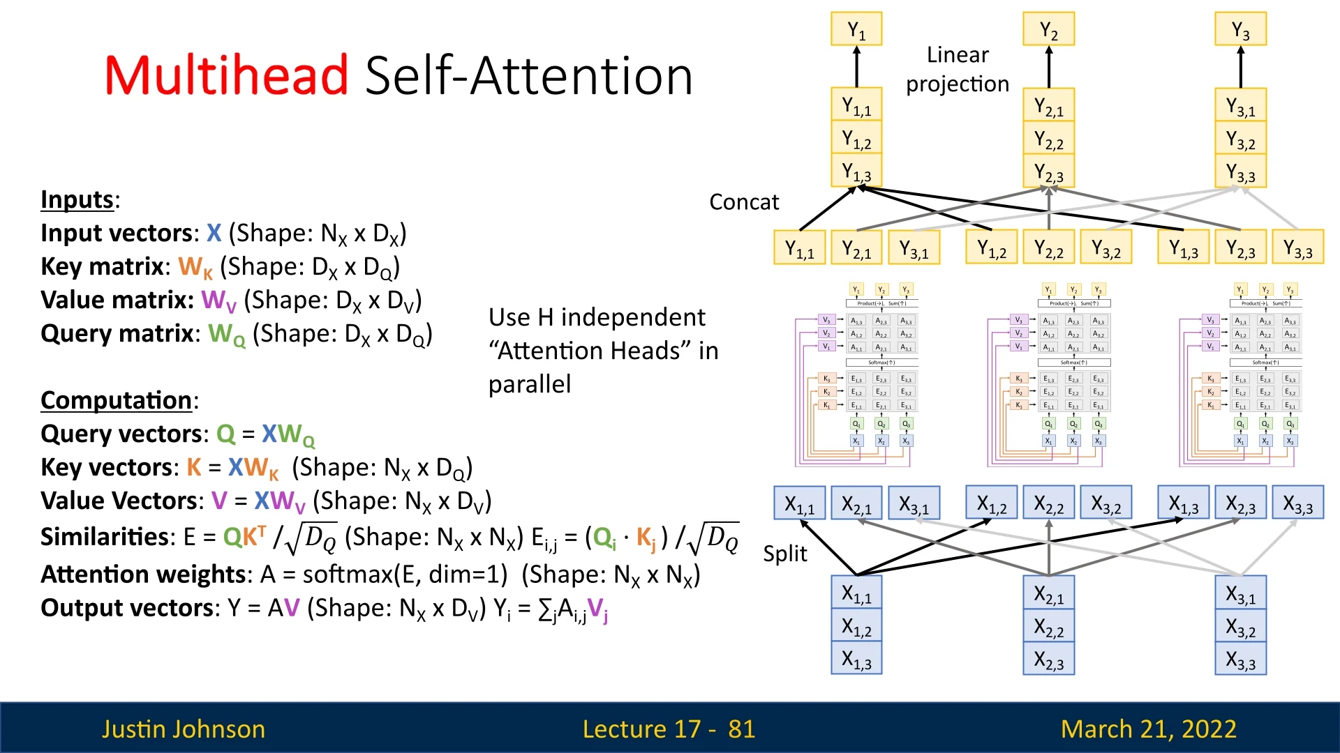
To integrate information across all heads, we apply a final linear transformation using a learned weight matrix \( W^O \):
\[ \mbox{MultiHead}(\mathbf {Q},\mathbf {K},\mathbf {V}) = \mbox{Concat}\left (\mbox{head}_1,\dots ,\mbox{head}_H\right ) W^O. \]
The matrix \( W^O \in \mathbb {R}^{D_{\mbox{model}} \times D_{\mbox{model}}} \) serves to mix the information from different heads, allowing the network to learn how to best combine the different attention representations. Without this projection, the different heads would contribute independently, rather than forming a cohesive final representation.
Optimized Implementation and Linear Projection
A naive implementation would require performing separate matrix multiplications for each attention head. However, this is computationally expensive. Instead, a common trick is to stack the weight matrices across all heads into a single large matrix:
- Instead of applying separate transformations for each head, we stack all \( W_h^Q, W_h^K, W_h^V \) into one large matrix \( W^Q, W^K, W^V \) of shape \( \mathbb {R}^{D_{\mbox{model}} \times H d_{\mbox{head}}} \).
- We then perform a single matrix multiplication to produce all query, key, and value matrices at once.
- These are then reshaped and split across heads.
This approach significantly reduces the number of matrix multiplications required, improving computational efficiency while maintaining the same functionality. The final concatenated representation is then transformed back into the original feature space using \( W^O \), ensuring that the model maintains the same output dimensionality as the input.
PyTorch Implementation of Multi-Head Attention
import torch
import torch.nn.functional as F


class MultiHeadSelfAttention(torch.nn.Module):
def __init__(self, dim_model, num_heads):


super().__init__()
assert dim_model % num_heads == 0, "D_model must be divisible by num_heads"
self.num_heads = num_heads
self.d_head = dim_model // num_heads

# Combine all heads’ Q, K, V projections into a single large matrix
self.W_qkv = torch.nn.Linear(dim_model, dim_model * 3, bias=False)
self.W_o = torch.nn.Linear(dim_model, dim_model, bias=False)


def forward(self, X):


batch_size, seq_len, dim_model = X.shape

# Compute Q, K, V using a single matrix multiplication
QKV = self.W_qkv(X)  # Shape: [B, L, 3 * D_model]
Q, K, V = torch.chunk(QKV, 3, dim=-1)  # Split into three parts

# Reshape for multi-head processing
Q = Q.view(batch_size, seq_len, self.num_heads, self.d_head).transpose(1, 2)
K = K.view(batch_size, seq_len, self.num_heads, self.d_head).transpose(1, 2)
V = V.view(batch_size, seq_len, self.num_heads, self.d_head).transpose(1, 2)

# Compute scaled dot-product attention
scores = torch.matmul(Q, K.transpose(-2, -1)) / self.d_head**0.5
weights = F.softmax(scores, dim=-1)
heads = torch.matmul(weights, V)  # Shape: [B, H, L, d_head]

# Concatenate heads and apply final linear projection
heads = heads.transpose(1, 2).contiguous().view(batch_size, seq_len, dim_model)
return self.W_o(heads)  # Output shape: [B, L, D_model]
Stepping Stone to Transformers and Vision Applications
Multi-head self-attention is a fundamental component of modern deep learning models and serves as the core mechanism in the Transformer architecture [664]. While self-attention allows a model to compute token interactions in parallel, multi-head attention enhances its capacity by attending to different parts of the sequence simultaneously.
However, before diving into how multi-head self-attention integrates into the Transformer, it is insightful to explore its applicability beyond sequence data. Especially in our domain, that is computer vision, where self-attention has been successfully integrated into convolutional architectures to enhance feature representation. This approach demonstrates the versatility of self-attention and offers valuable insights into its practical use cases.
17.5.10 Self-Attention for Vision Applications
Consider an input image processed by a convolutional neural network (CNN), yielding a feature map with dimensions \( C \times H \times W \), where \( C \) denotes the number of channels, and \( H \) and \( W \) represent the spatial height and width, respectively.
Generating Queries, Keys, and Values To apply self-attention within the CNN framework, we first generate the queries (\(Q\)), keys (\(K\)), and values (\(V\)) using separate \(1 \times 1\) convolutional layers, each with its distinct set of weights and biases. This approach ensures that spatial information is preserved while enabling efficient projection to a lower-dimensional space for computational efficiency. The transformations are given by:
\[ Q = W_Q * X + b_Q, \quad K = W_K * X + b_K, \quad V = W_V * X + b_V, \]
where:
- \( X \in \mathbb {R}^{C \times H \times W} \) is the input feature map.
- \( W_Q, W_K, W_V \in \mathbb {R}^{C' \times C \times 1 \times 1} \) are the convolutional weight matrices.
- \( b_Q, b_K, b_V \in \mathbb {R}^{C'} \) are the corresponding biases.
- \( C' \) is a reduced dimension for computational efficiency.
Notably, the spatial dimensions \(H\) and \(W\) remain unchanged, ensuring that each location in the query and key feature maps directly corresponds to a spatial location in the original input tensor. Each such location represents a specific window in the original image, as determined by the effective receptive field of the CNN layers.
Reshaping for Attention Computation After projection, each of \(Q\), \(K\), and \(V\) is reshaped to a two-dimensional form \( C' \times N \), where \( N = H \times W \) is the total number of spatial positions. This reshaping prepares the data for the attention computation:
\[ Q' \in \mathbb {R}^{C' \times N}, \quad K' \in \mathbb {R}^{C' \times N}, \quad V' \in \mathbb {R}^{C' \times N}. \]
Computing Attention Scores To compute attention, we transpose the queries along the spatial dimension, resulting in \( (Q')^\top \in \mathbb {R}^{N \times C'} \). This alignment ensures correct matrix multiplication for similarity computation. The attention score matrix is then calculated as:
\[ S = (Q')^\top K' \in \mathbb {R}^{N \times N}, \]
where each element \( S_{(i,j),(k,l)} \) measures the similarity between spatial position \((i,j)\) in the query and position \((k,l)\) in the key.
According to the dot-product attention formula, we scale the scores by \( \sqrt {C'} \) to mitigate the variance growth due to high-dimensional feature vectors:
\[ S = \frac {(Q')^\top K'}{\sqrt {C'}}. \]
Each spatial location is represented by a feature vector of length \( C' \), and the dot product between two such vectors grows with \( C' \). Scaling by \( \sqrt {C'} \) ensures that the variance of the similarity scores remains stable, thereby preventing softmax saturation and enabling smoother gradient flows during training, as suggested by Zhang et al. [784].
Normalizing Attention Weights Applying the softmax function along the last dimension ensures that attention scores sum to one:
\[ A = \mbox{softmax}(S) \in \mathbb {R}^{N \times N}. \]
Computing the Attention Output The output of the self-attention mechanism is computed by weighting the value vectors using the attention matrix:
\[ O' = V' A^\top \in \mathbb {R}^{C' \times N}. \]
This allows each spatial location to incorporate contextual information from all other locations, effectively capturing long-range dependencies that traditional convolutions might miss.
Reshaping, Final Projection, and Residual Connection The attention output \( O' \) is reshaped back to \( C' \times H \times W \). To align the dimensionality with the original feature map, we apply an additional \(1 \times 1\) convolution to project it back to \( C \) channels:
\[ O = W_O * \mbox{reshape}(O') + b_O \in \mathbb {R}^{C \times H \times W}, \]
where:
- \( W_O \in \mathbb {R}^{C \times C' \times 1 \times 1} \) is the final projection matrix.
- \( b_O \in \mathbb {R}^C \) is the corresponding bias.
Sometimes, a residual connection is added by summing the original input feature map \(X\) with the output of the attention mechanism:
\[ O_{\mbox{final}} = O + X. \]
This addition helps the model to retain original low-level information and prevents degradation in deeper architectures. Residual connections are particularly beneficial when the attention mechanism might overly focus on irrelevant positions or when the model struggles to refine feature representations effectively.
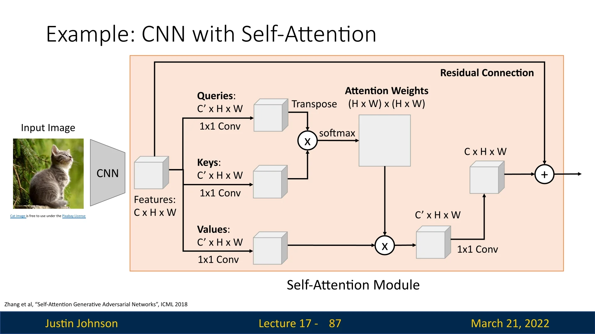
Summary This process effectively integrates self-attention into the CNN pipeline, enabling the model to capture long-range dependencies across spatial regions. By combining self-attention with convolution, the model benefits from both local feature extraction and global context awareness—qualities that are essential for tasks like image recognition and segmentation.
Bridging Towards Transformers
This example demonstrates the versatility of self-attention, extending its utility beyond sequences to spatial data. The ability to model complex relationships within an input—whether in sequences or images—highlights why self-attention has become a cornerstone of modern architectures.
In the next section, we explore how stacking multi-head self-attention layers with feed-forward networks forms the hierarchical structure of the Transformer. This architecture not only leverages the strengths of attention but also introduces mechanisms for deeper feature learning and improved generalization.
17.6 Transformer
17.6.1 Motivation and Introduction
The development of the Transformer architecture marked a pivotal moment in deep learning, fundamentally changing how models process sequential data. Introduced in the seminal paper ”Attention is All You Need” [664], Transformers replaced recurrence and convolutions with self-attention mechanisms, enabling unprecedented parallelism and flexibility in modeling long-range dependencies.
Before delving into the architectural details of Transformers, it’s important to understand the landscape of sequence processing methods that preceded them. In this section, we compare three prominent approaches for handling sequences: Recurrent Neural Networks (RNNs), 1D Convolutions, and Self-Attention. Each offers unique advantages and drawbacks, and understanding these will shed light on why the Transformer architecture was such a breakthrough.
Three Ways of Processing Sequences
Recurrent Neural Networks (RNNs) RNNs have been a foundational approach for processing ordered sequential data, such as text, audio, or time-series. They process input sequences step by step, maintaining a hidden state that captures information from previous time steps.
- Access to Full Temporal Receptive Field: In a single forward pass, the final hidden state \( h_T \) theoretically has access to the entire sequence. Each hidden state \( h_t \) is conditioned on all previous states, granting RNNs a full temporal receptive field.
- Limited Contextual Retention for Long Sequences: Despite this theoretical access, RNNs often struggle to retain long-range dependencies. The limited capacity of \( h_T \), combined with vanishing gradients, restricts the amount of earlier information that can be preserved, reducing the model’s ability to capture distant relationships effectively.
- Not Parallelizable: RNNs process sequences sequentially, where each hidden state depends on the previous one. This inherent dependency restricts parallelism and slows down training and inference.
1D Convolution for Sequence Processing 1D convolutions provide an efficient and parallelizable approach for handling sequential data, including time-series, audio signals, and natural language text. For scalar inputs like audio signals, 1D convolutions process sequences by sliding a filter across the sequence. For text, each word or token is first embedded into a high-dimensional vector. The convolutional filter then slides over this sequence of embeddings, applying learned weights to capture local patterns within subsequences of tokens. For example, a filter of size \(k\) processes \(k\)-length windows, enabling the model to detect local structures such as word pairs, phrases, or syntactic dependencies. This mechanism is analogous to how convolutional filters scan spatial regions in images, but adapted for sequential data.
- Highly Parallel: Unlike RNNs, convolutions process all positions in parallel. Each output can be computed independently, enabling efficient computation on modern hardware and accelerating both training and inference.
- Limited Temporal Receptive Field for Long Sequences: A single convolutional layer can only capture patterns within its filter size, meaning it is restricted to short-range dependencies. To model long-range interactions, multiple layers must be stacked, gradually expanding the receptive field. However, this increases model depth and complexity. Even with deeper stacks, convolutions can still struggle with extremely long sequences unless techniques like dilation are applied.
While 1D convolutions offer significant parallelization advantages and excel at capturing local patterns, their inability to capture long-range dependencies efficiently poses challenges for tasks like language modeling. Understanding relationships across distant tokens requires deeper architectures or additional techniques. This limitation motivates the need for architectures like self-attention and Transformers, which can inherently model global dependencies in a single layer.
Self-Attention Mechanism Self-attention introduces a fundamentally different approach by treating inputs as sets of vectors and learning dependencies between them without relying on sequential processing.
- Good at Long Sequences: After just one self-attention layer, each output token has access to the entire input sequence. This makes self-attention highly effective at capturing long-range dependencies.
- Highly Parallel: Self-attention operates through matrix multiplications, enabling all outputs to be computed in parallel. This dramatically accelerates training and inference.
- Memory Intensive: The primary drawback of self-attention is its memory and computational cost. Since it computes pairwise interactions between all tokens, its complexity scales quadratically with sequence length, posing challenges for very long sequences.
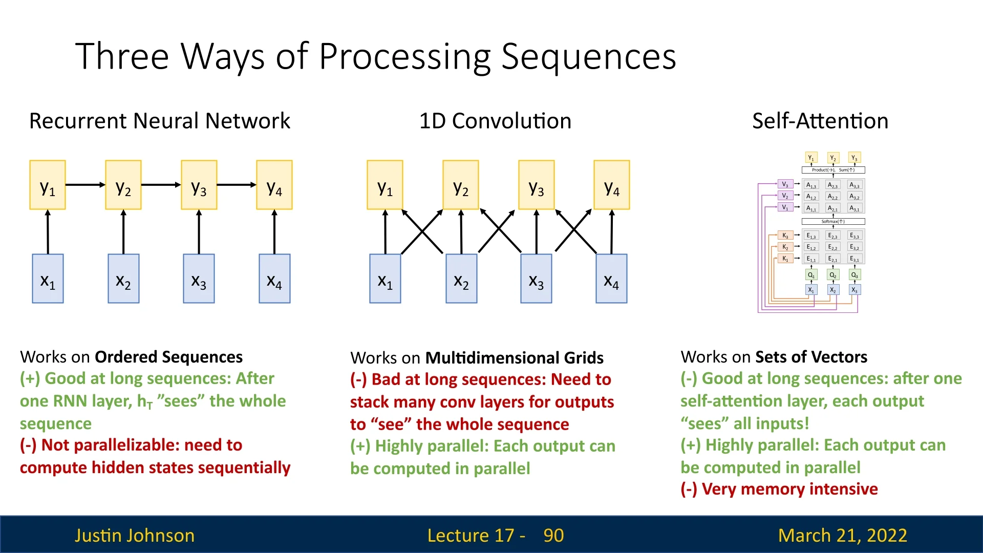
17.6.2 Why the Transformer?
Traditional sequence-to-sequence models follow an encoder-decoder architecture, where the encoder processes an input sequence into a latent representation, and the decoder autoregressively generates the output sequence using both this representation and previously generated tokens.
The Transformer architecture, introduced in “Attention is All You Need” [664], eliminated recurrence and convolutions, replacing them with a stack of self-attention-based encoder and decoder blocks. This design enabled fully parallelized processing, significantly improving efficiency while maintaining the ability to model long-range dependencies.
Later Transformer models, such as BERT and GPT, streamlined this approach by discarding the explicit encoder-decoder structure. Instead, they employed a stack of identical Transformer blocks—either encoder-only (e.g., BERT [121]) for bidirectional representation learning or decoder-only (e.g., GPT [511]) for autoregressive text generation. This evolution demonstrated that a single, unified Transformer block, rather than a separate encoder-decoder architecture, was sufficient for state-of-the-art performance across a wide range of sequence-based tasks.
In the following parts, we first examine the original encoder-decoder Transformer architecture 17.20 before proceeding to discuss the transition to the Transformer block, which serves as the foundation for modern architectures.
17.6.3 Seq2Seq Original Transformer Workflow
The original Transformer [664] is introduced in the context of sequence-to-sequence (seq2seq) machine translation with an encoder–decoder design. At a conceptual level, it solves the same problem as classical RNN/LSTM-based seq2seq systems: given a source sequence \(x_{1:M}\) (e.g., French), produce a target sequence \(y_{1:T}\) (e.g., English). The key difference is how the two halves compute and exchange information.
In an RNN/LSTM encoder, the hidden state is updated sequentially: \( h_t = f(h_{t-1}, x_t), \) so the number of computation steps grows with \(M\). In the Transformer encoder, the source tokens are processed in parallel within each layer: self-attention lets all tokens interact simultaneously, and stacking \(N\) blocks yields progressively more contextual representations. The decoder remains autoregressive at inference time in both families, but the Transformer decoder can be trained in parallel thanks to masking, which is a major practical and conceptual distinction.
We now walk through the original workflow from input to output. To keep the notation concrete, let \(d_{\mbox{model}}\) be the model dimension, \(M\) the source length, and \(T\) the target length. We denote the encoder output by \( H_{\mbox{enc}} \in \mathbb {R}^{M \times d_{\mbox{model}}}. \)
- 1.
- Tokenization & embedding. The source sentence is split into tokens and mapped to vectors \( \mathbf {x}_t \in \mathbb {R}^{d_{\mbox{model}}}. \) As in all embedding-based models, the goal is to learn semantic geometry in vector space, so that similarity reflects meaning rather than surface form.
- 2.
- Positional encoding. Since self-attention is order-agnostic, we add a positional signal to each token embedding: \[ \tilde {\mathbf {x}}_t = \mathbf {x}_t + \mathbf {p}_t \quad \mbox{(sinusoidal)} \qquad \mbox{or} \qquad \tilde {\mathbf {x}}_t = \mathbf {x}_t + \mathbf {P}_t \quad \mbox{(learned)}. \] This ensures that identical tokens appearing at different indices can be distinguished (Section 17.5.4).
- 3.
- Encode (parallel source contextualization). The full matrix of source representations \( \tilde {X} \in \mathbb {R}^{M \times d_{\mbox{model}}} \) is passed through \(N\) encoder blocks. Each block contains multi-head self-attention, an MLP, residual connections, and normalization. The output \( H_{\mbox{enc}} = \mbox{Encoder}(\tilde {X}) \) contains one vector per source token. Critically, each \(H_{\mbox{enc},i}\) is contextual: it is no longer just a representation of \(x_i\), but a representation of \(x_i\) as used in this sentence.
- 4.
- Decode (autoregressive target generation). The decoder is
also a stack of \(N\) blocks, but its role is fundamentally different
from the encoder. Where the encoder builds a static, fully parallel
representation of the entire source, the decoder constructs the target
sequence autoregressively at inference time. Each decoder block
contains three sublayers:
- Masked self-attention. Models dependencies among the already generated target tokens. A causal (look-ahead) mask ensures that the representation at position \(t\) can attend only to positions \(\le t\). This prevents the decoder from using future target information while still allowing full parallel computation across target positions during training.
- Cross-attention. Aligns the current target prefix with the full encoded source. This is the main channel through which source information enters the target-side computation.
- Position-wise FFN (MLP). Applies a position-wise nonlinear transformation that refines the fused representation.
How cross-attention turns French memory into English predictions. A common source of confusion is that the cross-attention values \(V\) are derived from encoder states that represent French tokens.
How, then, can the decoder use them to predict an English word? The answer is that cross-attention does not output a French word; it outputs a semantic context vector that is fused with the decoder’s English-side state.
Formally, if \(S \in \mathbb {R}^{t \times d_{\mbox{model}}}\) denotes the decoder hidden states for the current target prefix of length \(t\), then cross-attention uses: \[ Q = S W_Q, \qquad K = H_{\mbox{enc}} W_K, \qquad V = H_{\mbox{enc}} W_V, \] where \(H_{\mbox{enc}} \in \mathbb {R}^{M \times d_{\mbox{model}}}\) is the encoder output. The attention output is: \[ \mbox{Attn}(Q,K,V) = \mbox{softmax}\!\left (\frac {QK^\top }{\sqrt {d_k}}\right )V. \] Intuitively, \(Q\) represents what the decoder needs next in English, while \(K\) and \(V\) represent what meaning is available in the French source. The weighted sum over \(V\) therefore acts like a retrieved meaning snippet.
Crucially, this retrieved vector is then combined with the decoder stream through the residual pathway: the decoder state after cross-attention becomes a hybrid representation that encodes both (i) the target-side syntactic and contextual requirements and (ii) the source-side semantic content. The subsequent MLP and the final vocabulary projection are trained to map this hybrid representation into the target-language vocabulary. Thus, the model is not selecting a French word from \(V\); it is using \(V\) to enrich an English decoder state that is already positioned to predict an English token.
Masks, autoregression, and training efficiency. At inference, the decoder is unavoidably sequential: we generate \(y_1\), feed it back, then generate \(y_2\), and so on. This matches the autoregressive factorization: \[ p(y_{1:T}\mid x_{1:M}) = \prod _{t=1}^{T} p(y_t \mid y_{<t}, x_{1:M}). \] At training, however, we can compute all conditional terms in parallel using teacher forcing: the decoder receives the shifted ground-truth sequence \([\texttt{<BOS>}, y_1, \dots , y_{T-1}]\), while the causal mask prevents position \(t\) from attending to \(>t\). This preserves the same autoregressive objective without cheating, but allows the entire target sequence to be processed in a single forward pass.
This is more efficient than RNN/LSTM decoders for two reasons:
- Even with teacher forcing, an RNN/LSTM decoder must still be unrolled in time, so the training computation contains an irreducible sequential chain of length \(T\).
- The Transformer decoder replaces this temporal dependency with masked attention, so the per-layer computation is dominated by parallel matrix operations that exploit GPU throughput.
- 5.
- Projection & softmax. After the final decoder block, each position
produces logits over the target vocabulary. Let \(\mathbf {y}_t\) denote the decoder’s final
hidden state at step \(t\) after the full decoder stack.
\[ \mathbf {z}_t = \mathbf {y}_t W_{\mbox{vocab}} + \mathbf {b}, \qquad p(y_t \mid y_{<t}, x_{1:M}) = \mbox{softmax}(\mathbf {z}_t), \] Training minimizes the standard autoregressive negative log-likelihood: \[ \mathcal {L} = -\sum _{t=1}^{T} \log p(y_t \mid y_{<t}, x_{1:M}). \]
Toy Translation Example: “Je suis étudiant” \(\rightarrow \) “I am a student”
Consider the source tokens: \[ x_{1:3} = [\mbox{Je}, \mbox{suis}, \mbox{\'{e}tudiant}], \] and the target tokens: \[ y_{1:4} = [\mbox{I}, \mbox{am}, \mbox{a}, \mbox{student}]. \]
Encoder outcome After embedding and positional encoding, the encoder produces \[ H_{\mbox{enc}} = [H_{\mbox{Je}}, H_{\mbox{suis}}, H_{\mbox{\'{e}tudiant}}] \in \mathbb {R}^{3 \times d_{\mbox{model}}}. \] These are contextual source vectors. For instance, \(H_{\mbox{suis}}\) represents “suis as used after Je” and thus already encodes the first-person present-tense verb meaning, while \(H_{\mbox{\'{e}tudiant}}\) represents a noun functioning as a predicate complement in this clause.
Importantly, the encoder is allowed to see the entire source sentence. This is not a form of leakage: machine translation models are trained to approximate \(p(y_{1:T}\mid x_{1:M})\), and the conditioning sequence \(x_{1:M}\) is fully observed before any target token is generated. Thus, using all of \(H_{\mbox{enc}}\) in cross-attention is exactly the intended problem setup.
Decoder inference (autoregression) During inference, the decoder generates tokens sequentially. Let <BOS> be a start token. At step \(t\), the decoder consumes the prefix \(y_{<t}\), applies masked self-attention over this prefix, and then uses cross-attention to retrieve the most relevant source meaning from \(H\). The English word itself is not produced inside cross-attention; instead, cross-attention injects source-side meaning into the target-side state. The final word is selected by the vocabulary projection at the top of the decoder stack.
- Step 1. Input prefix: \([\texttt{<BOS>}]\). Masked self-attention is trivial. The cross-attention query derived from the start state typically aligns with \(H_{\mbox{Je}}\), retrieving a representation of the first-person subject. This retrieved meaning is fused with the decoder state via the residual pathway and refined by the block MLP. The final Linear+Softmax head then predicts \(\mbox{I}\).
- Step 2. Input prefix: \([\texttt{<BOS>}, \mbox{I}]\). Masked self-attention forms an English-side context that strongly expects a verb. Cross-attention emphasizes \(H_{\mbox{suis}}\), retrieving the “to be” meaning aligned with the subject. After fusion and refinement, the vocabulary head predicts \(\mbox{am}\).
- Step 3. Input prefix: \([\texttt{<BOS>}, \mbox{I}, \mbox{am}]\). Cross-attention can already draw meaning from \(H_{\mbox{\'{e}tudiant}}\), but the decoder’s target-language modeling components (masked self-attention history and MLPs) capture an English syntactic regularity: many singular count nouns require an article. The vocabulary head therefore predicts \(\mbox{a}\).
- Step 4. Input prefix: \([\texttt{<BOS>}, \mbox{I}, \mbox{am}, \mbox{a}]\). The decoder state now represents an “article awaiting a noun” context. Cross-attention assigns high weight to \(H_{\mbox{\'{e}tudiant}}\). The fused representation maps cleanly into the English vocabulary, leading to the prediction \(\mbox{student}\), followed by <EOS>.
This illustrates the functional division: the encoder builds a parallel, contextual memory of the entire source, while the decoder provides the target-language scaffold and repeatedly retrieves source meaning. Cross-attention is therefore best viewed as meaning retrieval and fusion, not as a direct “French-to-English dictionary” layer. The actual English token is selected by the final decoder representation after it has been shaped jointly by masked self-attention, cross-attention, and MLP refinement.
Teacher Forcing: Training the Autoregressive Decoder in Parallel
A central practical idea in seq2seq training is teacher forcing. As in RNN decoders, the objective is to learn \[ p(y_t \mid y_{<t}, x_{1:M}). \] The key difference in Transformers is that teacher forcing combines naturally with causal masking to enable parallel training over all target positions.
What teacher forcing actually does During training, the model does not feed its own sampled predictions back into the next step. Instead, it always conditions on the ground-truth prefix. Concretely, we shift the target sequence right: \[ \mbox{Decoder input: } [\texttt{<BOS>}, y_1, y_2, \dots , y_{T-1}], \qquad \mbox{Targets: } [y_1, y_2, \dots , y_T]. \] Even if the model would have predicted the wrong word at position \(t\), we still:
- Compute the loss for that error.
- Provide the correct token \(y_t\) as part of the input prefix for predicting \(y_{t+1}\).
Thus, teacher forcing decouples learning the conditional distribution at step \(t\) from the model’s own potentially noisy intermediate rollouts. The model is trained to be accurate under correct target-side histories.
How masking works efficiently in self-attention A natural concern is that self-attention is defined over all query–key pairs, so feeding the full teacher-forced target sequence seems to allow “future leakage”. The key point is that Transformers do not avoid computing the full score matrix; they compute it once in parallel and then nullify illegal interactions before the softmax.
Let \(S \in \mathbb {R}^{T \times d_{\mbox{model}}}\) denote the decoder input embeddings after adding positional information. In a masked self-attention sublayer, we form \[ Q = S W_Q, \qquad K = S W_K, \qquad V = S W_V, \] and compute the raw score matrix \[ A = \frac {QK^\top }{\sqrt {d_k}} \in \mathbb {R}^{T \times T}. \] These scores \(A_{ij}\) are computed for all pairs \((i,j)\) via a single matrix multiplication, which is highly optimized on GPUs.
We then add a causal mask \(M\), where \[ M_{ij} = \begin {cases} 0, & j \le i,\\ -\infty , & j > i, \end {cases} \] to obtain \[ \tilde {A} = A + M. \] Applying softmax row-wise yields attention weights \[ \alpha _{i:} = \mbox{softmax}(\tilde {A}_{i:}), \] so that all entries with \(j > i\) become exactly zero. Thus, token \(i\) can only attend to itself and earlier tokens, even though the computation was performed in one parallel pass. The masked output is \[ \mbox{MSA}(S) = \alpha V. \] This is the crucial implementation trick: we preserve the autoregressive factorization by masking, not by making the computation sequential [664].
Why this is more efficient than RNN/LSTM training With teacher forcing, an RNN/LSTM decoder still requires sequential unrolling: even though the ground-truth tokens are known, the hidden state update \(h_t = f(h_{t-1}, y_{t-1})\) forces a length-\(T\) dependency chain. In contrast, the Transformer decoder can compute all \(T\) position-wise losses in a single forward pass dominated by parallel matrix operations (\(QK^\top \), masked softmax, and \(\alpha V\)). This difference is one of the main reasons Transformers train faster and scale better in practice.
A note on exposure bias Teacher forcing introduces a mild train–test mismatch: during training, the decoder conditions on perfect prefixes, while at inference it conditions on its own sampled outputs. This phenomenon, called exposure bias, implies that recovery from early mistakes is not explicitly practiced during standard training. Despite this caveat, teacher forcing remains the standard baseline because of its stability and efficiency.
Decoding Strategies at Inference
At inference time, ground-truth target tokens are unavailable, so teacher forcing cannot be used. Given a source sequence \(x_{1:M}\), the decoder produces a distribution \( p(y_t \mid y_{<t}, x_{1:M}) \) at each step. The ideal goal is to find the target sentence with maximum joint probability: \[ y_{1:T}^\star = \arg \max _{y_{1:T}} \sum _{t=1}^{T} \log p(y_t \mid y_{<t}, x_{1:M}), \] but exact search is intractable for realistic vocabularies. We therefore use practical decoding heuristics.
Greedy decoding Greedy decoding chooses the locally most probable token at each step: \[ y_t = \arg \max _{w} \; p(w \mid y_{<t}, x_{1:M}). \]
- Strength. Very fast and simple.
- Limitation. Short-sighted: once a token is chosen, the algorithm cannot reconsider it, so an early locally optimal choice may lead to a worse full sentence.
Beam search Beam search is the standard decoding strategy for many deterministic seq2seq tasks, especially machine translation. Instead of committing to a single prefix, it maintains the top \(B\) partial hypotheses (the beam) according to cumulative log-probability. At each step, it:
- 1.
- Expands every beam hypothesis with candidate next tokens.
- 2.
- Scores the resulting extended sequences by cumulative log-probability.
- 3.
- Retains the best \(B\) sequences as the new beam.
This approximates a more global search than greedy decoding.
A small concrete example (Beam vs. Greedy) Consider our toy translation \( \textit {``Je suis \'{e}tudiant''} \rightarrow \textit {``I am a student''} \), with beam width \(B=2\). We show a simplified probability pattern for illustration.
- Step 1 (predict first token). Given \([\texttt{<BOS>}]\), suppose: \[ p(\mbox{I})=0.60, \quad p(\mbox{Me})=0.30, \quad p(\mbox{Others}) \ll 1. \] Greedy picks \([\mbox{I}]\). Beam keeps two hypotheses: \([\mbox{I}]\) and \([\mbox{Me}]\), with scores \(\log 0.60\) and \(\log 0.30\).
- Step 2 (expand both hypotheses). Suppose the next-token distributions are: \[ p(\mbox{am}\mid \mbox{I})=0.90, \quad p(\mbox{have}\mid \mbox{I})=0.03, \] \[ p(\mbox{too}\mid \mbox{Me})=0.60, \quad p(\mbox{is}\mid \mbox{Me})=0.20, \quad p(\mbox{am}\mid \mbox{Me})=0.01. \] Beam forms candidates such as: \[ \log p(\mbox{I am}) = \log 0.60 + \log 0.90, \] \[ \log p(\mbox{Me too}) = \log 0.30 + \log 0.60, \] and keeps the top two overall, likely \([\mbox{I am}]\) and \([\mbox{Me too}]\).
- Step 3 (beam can recover). Suppose: \[ p(\mbox{a}\mid \mbox{I am})=0.70, \quad p(\mbox{student}\mid \mbox{I am})=0.10, \] while the continuation of \([\mbox{Me too}]\) is low-probability for this translation task. After rescoring and pruning, the beam will likely drop \([\mbox{Me too}]\) and keep hypotheses derived from \([\mbox{I am}]\), such as \([\mbox{I am a}]\).
- Step 4 (finish). From \([\mbox{I am a}]\), suppose: \( p(\mbox{student})=0.80 \), so the model outputs \([\mbox{I am a student}]\).
This illustrates the key difference: greedy decoding commits to one path immediately, while beam search delays commitment, keeping multiple plausible prefixes long enough to avoid mistakes that only become evident a few steps later.
Length normalization Because beam search sums log-probabilities, longer sequences can be unfairly penalized. A common fix is length normalization: \[ \mbox{Score}(y_{1:L}) = \frac {1}{L^\alpha } \sum _{t=1}^{L} \log p(y_t \mid y_{<t}, x_{1:M}), \] with \(\alpha \in [0,1]\). This discourages an artificial preference for overly short outputs.
Practical guidance In machine translation, modest beam widths (often \(B \approx 4\mbox{--}8\)) are common practical choices, balancing quality and runtime. Greedy decoding can be preferred for low-latency systems or when a small quality drop is acceptable.
Where sampling fits (briefly) Greedy decoding and beam search are deterministic: running them twice yields the same output. By contrast, sampling-based strategies (e.g., top-\(k\) or nucleus sampling) draw the next token stochastically from a restricted candidate set. They are more common in open-ended generation, where diversity and stylistic variation are desirable, and less common in standard translation benchmarks where faithfulness and consistency dominate the objective.
Summary: Transformer Seq2Seq vs. RNN/LSTM Seq2Seq
The original Transformer preserves the high-level encoder–decoder logic of earlier seq2seq systems, but changes the computational substrate:
- Encoder computation. RNNs build the source representation sequentially; Transformers build it in parallel through self-attention.
- Decoder training. RNN decoders are typically unrolled sequentially even with teacher forcing; Transformer decoders use teacher forcing plus a causal mask to compute all target-position losses in parallel.
- Alignment mechanism. Both families can use attention, but the Transformer’s multi-head cross-attention offers a flexible, highly parallel way to align target queries with a rich source memory at every decoding step.
This workflow explains why the original architecture in the following figure became the dominant template for neural machine translation and served as the foundation for later encoder-only and decoder-only variants.
From end-to-end workflow to the block-level “engine” The step-by-step seq2seq workflow above explains what the original Transformer computes: a parallel encoder that produces a contextual source memory \(H\), and an autoregressive decoder that repeatedly queries this memory to construct the target sequence. To fully understand why this design works—and why it scales so well compared to RNN/LSTM-based seq2seq—we now zoom in on the internal mechanics of the two atomic building blocks that realize this computation: the encoder block and the decoder block.
This shift in viewpoint is useful because the Transformer’s high-level behavior is an emergent property of a simple repeating pattern. In each encoder layer, self-attention provides global token-to-token communication, while the position-wise FFN provides local nonlinear refinement. In each decoder layer, masked self-attention enforces causal target-side coherence, cross-attention performs source meaning retrieval and fusion, and the FFN reshapes this fused signal into representations that the final vocabulary head can map into fluent English tokens.
We therefore present the encoder and decoder blocks next using the same notation as the workflow: \(d_{\mbox{model}}\) for the model dimension, \(X \in \mathbb {R}^{L \times d_{\mbox{model}}}\) for generic token representations, and \(H_{\mbox{enc}} \in \mathbb {R}^{M \times d_{\mbox{model}}}\) for the encoder’s source memory. This block-level analysis will also set up a clean conceptual bridge to modern architectures, where “encoder-style” and “decoder-style” behavior is produced by reusing the same block template with different attention masks and, in some cases, by removing cross-attention entirely.
Transformer Encoder Block: Structure and Reasoning
After constructing the input representations \( X \in \mathbb {R}^{L \times d_{\mbox{model}}} \) from token embeddings and positional encodings, the Transformer encoder refines them using a stack of \(N\) identical encoder blocks. Each block alternates between: (i) communication across tokens via multi-head self-attention, and (ii) nonlinear per-token processing via a position-wise feed-forward network (FFN). Residual connections and layer normalization stabilize both steps and enable deep stacking.
Using the notation of the previous sections, one encoder block can be summarized as: \begin {align} Z &= \text {LayerNorm}\!\bigl (X + \text {MultiHeadSelfAttn}(X)\bigr ), \\ Y &= \text {LayerNorm}\!\bigl (Z + \text {FFN}(Z)\bigr ), \end {align}
where \(Y \in \mathbb {R}^{L \times d_{\mbox{model}}}\) is the block output.
Multi-head self-attention: the “communication” step Self-attention updates each token representation by allowing it to aggregate information from all other tokens. For head \(h \in \{1,\dots ,n_h\}\), we form: \[ Q^{(h)} = XW_Q^{(h)}, \qquad K^{(h)} = XW_K^{(h)}, \qquad V^{(h)} = XW_V^{(h)}, \] and compute attention-weighted mixtures of \(V^{(h)}\) using the similarities between \(Q^{(h)}\) and \(K^{(h)}\). The head outputs are concatenated and projected back to \(d_{\mbox{model}}\).
Intuition. A single head would need to compress multiple kinds of relations into one pattern. Multiple heads allow the model to separate concerns. For example, in a sentence with pronouns, one head may specialize in linking a pronoun to its antecedent, while another captures predicate–argument structure. This division improves expressivity without requiring deeper layers to disentangle mixed signals.
Residual connection: the “information highway” The attention output is added to the original input \(X\) before normalization. This turns the sub-layer into a refinement mechanism: instead of rewriting representations from scratch, the block learns a correction to the current state.
Why it matters. In deep stacks, residual paths preserve gradients and prevent the early layers from being overwritten by noisy updates. A concrete mental model is: keep the current token meaning, then add whatever context the attention discovered. If attention learns little for a token in a given layer, the representation can still pass through largely unchanged.
Layer normalization: why it fits Transformers LayerNorm normalizes each token vector independently across its feature dimension: \[ \hat {z}_{i,j} = \frac {z_{i,j}-\mu _i}{\sqrt {\sigma _i^2+\epsilon }}, \qquad \mbox{LayerNorm}(z_i) = \gamma \cdot \hat {z}_i + \beta . \]
Why this works well here.
- Token-wise stability. Self-attention forms weighted sums whose magnitudes can vary substantially across layers and heads. LayerNorm resets the scale of each token representation, reducing the risk of activation drift as \(N\) grows.
- Robustness to variable lengths and padding. Unlike BatchNorm, which depends on batch statistics, LayerNorm does not become unstable when sequences have different lengths or when padding is present.
- Clean separation of roles. Attention defines who talks to whom; LayerNorm ensures that the resulting messages arrive at a consistent numerical scale, so later layers can rely on stable feature ranges.
Note: for historical alignment: the original Transformer uses the post-addition \(\mbox{LayerNorm}(X + \cdot )\) pattern shown above; many later variants adopt pre-norm for even easier optimization, but the conceptual roles remain the same.
Position-wise FFN: the “processing” step After tokens exchange information through attention, the FFN applies a nonlinear transformation to each token independently: \[ \mbox{FFN}(z_i) = \max (0, z_iW_1 + b_1)W_2 + b_2. \]
Intuition. Self-attention primarily mixes information across positions. The FFN then interprets and reshapes that mixed signal within each token. A short example: if attention makes a token embedding reflect both a word and its disambiguating context (e.g., “bank” strongly attending to “river”), the FFN can convert this combined evidence into a more decisive, nonlinear feature representation of the intended sense. Without the FFN, stacking attention layers would provide less expressive per-token transformation capacity.
Putting the pieces together Each encoder block therefore follows a consistent logic:
- Attention lets every token gather evidence from the sequence.
- Residuals preserve the original signal while adding context-driven updates.
- LayerNorm stabilizes scale and training across deep stacks.
- FFN injects nonlinearity and increases per-token representational power.
This balance between global interaction (attention) and local refinement (FFN), supported by stable optimization (residuals + LayerNorm), is the core computational template that makes Transformer encoders both expressive and scalable.
Transformer Decoder Block: Structure and Reasoning
The decoder block is the generative counterpart of the encoder block. It retains the same core design principles—attention for interaction, FFNs for per-token refinement, residual connections for stable signal flow, and LayerNorm for scale control—but introduces two decoder-specific requirements:
- 1.
- Enforce causal (autoregressive) generation on the target side.
- 2.
- Enable source–target alignment through encoder–decoder cross-attention.
Let the current target-side representations be \( X_{\mbox{dec}} \in \mathbb {R}^{T \times d_{\mbox{model}}} \), where \(T\) is the length of the (teacher-forced or partially generated) target prefix, and let the encoder output be \( H_{\mbox{enc}} \in \mathbb {R}^{M \times d_{\mbox{model}}} \) for a source sequence of length \(M\). One decoder block can be written compactly as: \begin {align} Z_{\text {dec}} &= \text {LayerNorm}\!\Bigl ( X_{\text {dec}} + \text {MaskedMultiHeadSelfAttn}(X_{\text {dec}}) \Bigr ), \\ C_{\text {dec}} &= \text {LayerNorm}\!\Bigl ( Z_{\text {dec}} + \text {MultiHeadCrossAttn}(Z_{\text {dec}}, H_{\text {enc}}) \Bigr ), \\ Y_{\text {dec}} &= \text {LayerNorm}\!\Bigl ( C_{\text {dec}} + \text {FFN}(C_{\text {dec}}) \Bigr ). \end {align}
Relative to the encoder, the decoder therefore adds one additional “bridge” sub-layer.
1. Masked multi-head self-attention: the “coherence” step The first sub-layer is self-attention over the target-side stream, but with a causal mask. This ensures that the representation at position \(t\) can only attend to positions \(\le t\). Operationally, the attention score matrix is computed in parallel and then masked before the softmax so that illegal (future) connections receive zero probability mass.
Intuition. This sub-layer is the decoder’s internal language-modeling engine. It enforces grammatical and semantic consistency within the partially formed English sentence. For example, after the prefix “I am”, masked self-attention helps the next position represent “a noun phrase is likely coming” without requiring any access to future tokens.
2. Cross-attention: the “bridge” to source meaning The second sub-layer retrieves information from the encoded source sequence. Here the decoder provides queries, while the encoder provides a fixed memory of keys and values: \[ Q = Z_{\mbox{dec}} W_Q, \qquad K = H_{\mbox{enc}} W_K, \qquad V = H_{\mbox{enc}} W_V. \]
Why this is not a contradiction in languages. A common conceptual confusion is: if \(V\) originates from French token representations, how can the model output an English word? The key is that the cross-attention output is not used as a word by itself. Instead, it is added to the decoder stream via a residual connection, producing a target-conditioned, source-enriched representation. That fused vector is then transformed by the FFN and, after the full decoder stack, projected into the English vocabulary space. In effect:
the encoder provides meaning, the decoder provides the English syntactic scaffold, and the final projection selects the English token that best matches the fused state.
Short example. In the toy translation \( \textit {``Je suis \'{e}tudiant''} \rightarrow \textit {``I am a student''}, \) the decoder state after \([\texttt{<BOS>}, \mbox{I}]\) represents “first-person subject; verb needed”. Cross-attention then retrieves the source evidence most aligned with this intent, often emphasizing the encoder vector for “suis”. The residual fusion produces a representation that encodes “English verb slot + source meaning of to be”, which the downstream transformations can map to “am”.
3. Position-wise FFN: the “processing” step As in the encoder, the FFN is applied independently to each position: \[ \mbox{FFN}(c_i) = \max (0, c_iW_1 + b_1)W_2 + b_2. \]
Intuition. Cross-attention is an information-retrieval mechanism. The FFN is where the model digests the retrieved evidence and reshapes it into a form that is useful for the next-token decision. It injects nonlinearity and capacity that pure attention mixing cannot provide.
4. Residual connections and LayerNorm: stability across deep stacks Each sub-layer is wrapped in Add+Norm. The residual path preserves the decoder’s current hypothesis while allowing incremental updates, and LayerNorm stabilizes the scale of token representations independently of batch statistics.
Why LayerNorm is especially important in the decoder. The decoder must balance two evolving information sources:
- The growing target prefix (masked self-attention).
- The fixed source memory (cross-attention).
LayerNorm keeps these signals numerically compatible across layers, preventing either stream from dominating due to scale drift. (As with the encoder, this description matches the post-norm pattern in the original Transformer).
5. Final token generation (after the decoder stack) A single block produces refined hidden states \(Y_{\mbox{dec}}\), but token prediction occurs after stacking \(N\) decoder blocks. Let \(\mathbf {y}_t\) denote the final hidden state at position \(t\) after the full decoder stack. We then compute: \[ \mathbf {z}_t = \mathbf {y}_t W_{\mbox{vocab}} + \mathbf {b}, \qquad p(y_t \mid y_{<t}, x_{1:M}) = \mbox{softmax}(\mathbf {z}_t). \]
This separation clarifies the roles: decoder blocks construct a meaningful latent representation, and the final linear projection + softmax select the English word.
Why this structure? The decoder block is designed to alternate between:
- Look back. Use masked self-attention to maintain target-side coherence without cheating.
- Look across. Use cross-attention to retrieve the relevant source meaning.
- Refine. Use the FFN to convert fused evidence into a sharper per-token representation.
This is the minimal architectural extension of the encoder block that makes autoregressive, source-conditioned generation possible, and it explains why the original encoder–decoder Transformer can be trained efficiently with teacher forcing while still behaving as a strictly causal generator at inference time.
17.6.4 The Modern Unified Transformer Block
The original Transformer [664] was introduced for machine translation, a task that naturally motivates an explicit encoder–decoder split: the encoder produces a fully observed source memory, and the decoder generates a target sequence autoregressively while querying that memory. As Transformers expanded beyond translation into large-scale language understanding and single-stream generation, the field increasingly recognized that the original encoder block and decoder block are best viewed as configurations of a shared architectural template.
Modern architectures therefore often adopt a unified Transformer block: a standardized building block based on the same high-level logic, self-attention + FFN + residual connections + normalization. In this view, the model family is determined primarily by (i) the self-attention mask and (ii) whether an explicit cross-attention bridge is added when source-conditioned generation is required.
Structure of the Modern Block (Pre-Norm)
At the block level, modern Transformers standardize computation into a two-stage refinement pattern: a communication step across tokens followed by a per-token processing step. Unlike the original post-norm formulation (Add \(\rightarrow \) Norm), contemporary large-scale systems commonly prefer a Pre-Norm ordering to improve optimization stability in deep stacks.
Let the token matrix be \( X \in \mathbb {R}^{L \times d_{\mbox{model}}}. \) A modern block produces \( Y \in \mathbb {R}^{L \times d_{\mbox{model}}} \) via: \begin {align} Z &= X + \text {MultiHeadSelfAttn}(\text {LayerNorm}(X)), \\ Y &= Z + \text {FFN}(\text {LayerNorm}(Z)). \end {align}
Conceptually, the roles remain consistent with the encoder–decoder analysis:
- 1.
- LayerNorm. Stabilizes the input to each sub-layer.
- 2.
- Self-attention. Performs global token-to-token communication.
- 3.
- FFN. Refines each token independently, typically by expanding to \(4d_{\mbox{model}}\) and projecting back.
- 4.
- Residual connections. Preserve signal flow and support deep stacking.
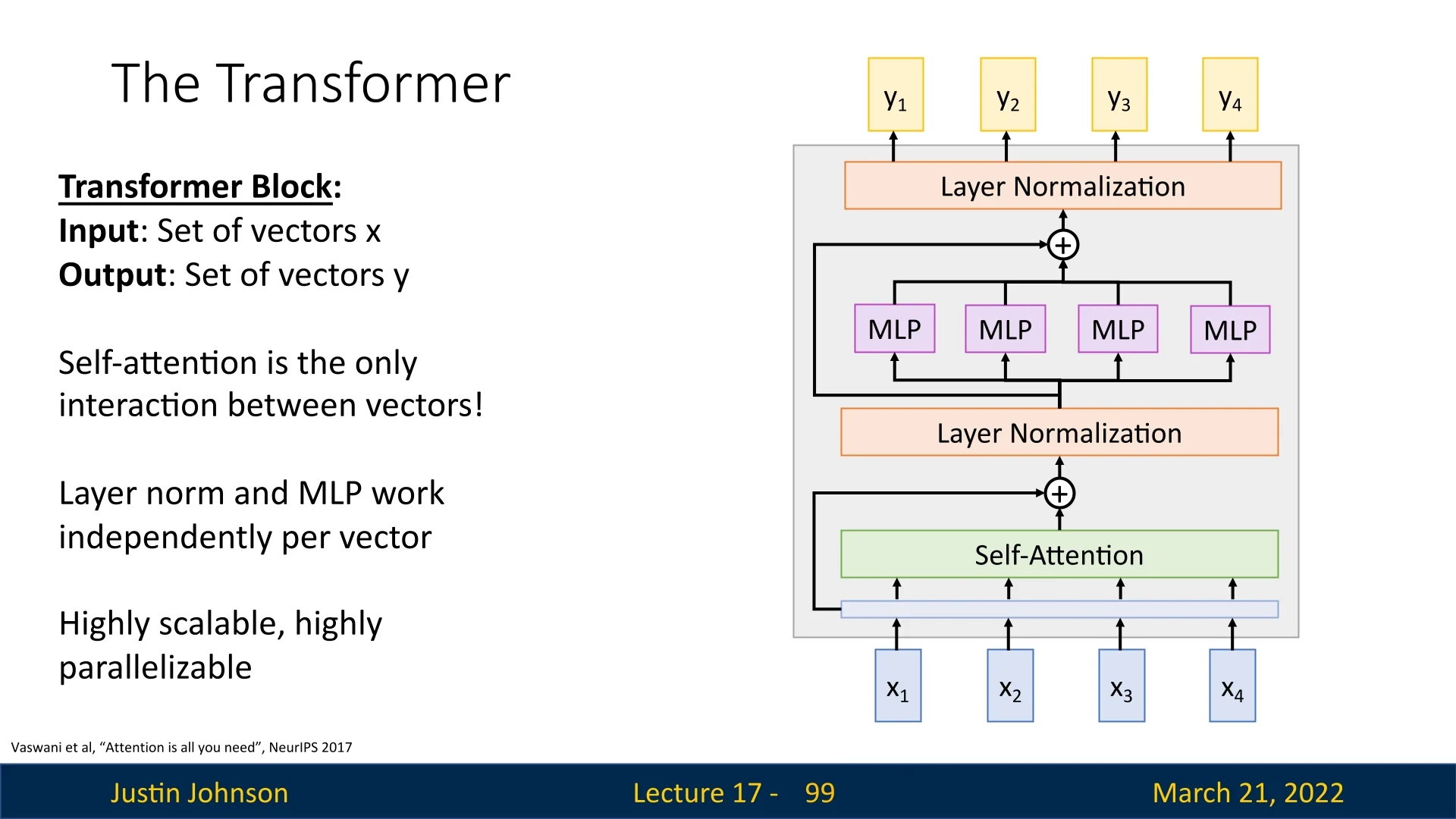
Three Model Families via Masking and Cross-Attention
By adjusting the self-attention mask and optionally enabling cross-attention, the unified block template yields the dominant architectural families:
- 1.
- Encoder-only models (bidirectional understanding). These models use unmasked self-attention, so every token can attend to every other token in the input. This configuration is well suited to tasks where the full sequence is observed and the goal is robust contextual representation learning (e.g., BERT-style pretraining and downstream classification).
- 2.
- Decoder-only models (causal generation). These models use causal masked self-attention, so token \(t\) can attend only to positions \(\le t\). The cross-attention sub-layer is removed entirely, yielding a single-stack autoregressive language model (e.g., GPT-style systems).
- 3.
- Encoder–decoder models (source-conditioned generation). This family retains the original separation: unmasked encoder self-attention builds a complete source memory, and the decoder combines masked self-attention with an explicit cross-attention bridge. This design remains a clean match for transduction problems such as translation and structured summarization (e.g., the original Transformer, T5).
This unifying view clarifies that modern architectures do not rely on new primitives: they reuse the same block-level machinery, and obtain different behaviors by controlling information access through masking and by adding cross-attention only when a distinct source sequence must be consulted.
PyTorch Implementation
The following PyTorch implementation illustrates the modern Pre-Norm block structure:
class ModernTransformerBlock(nn.Module):


def __init__(self, d_model, heads):


super().__init__()

self.norm1 = nn.LayerNorm(d_model)
self.attn = SelfAttention(d_model, heads=heads)

self.norm2 = nn.LayerNorm(d_model)
self.ff = nn.Sequential(
    nn.Linear(d_model, 4 * d_model),
    nn.GELU(),
    nn.Linear(4 * d_model, d_model),
)


def forward(self, x, mask=None):


    # Pre-Norm self-attention + residual
x = x + self.attn(self.norm1(x), mask=mask)

# Pre-Norm FFN + residual
x = x + self.ff(self.norm2(x))
return x
Key points in the implementation:
- The FFN expands to \(4d_{\mbox{model}}\) and projects back, a widely used capacity pattern in both encoder-only and decoder-only families.
- The Pre-Norm pattern normalizes inputs to each sub-layer, improving stability when stacking many blocks.
- Aside from self-attention, computations are token-wise, which preserves parallel efficiency across positions.
Why the Shift to Unified Blocks?
Treating the Transformer block as a general-purpose computational primitive enabled a major simplification in model design. Rather than designing distinct internal machinery for each task, modern systems largely reuse the same block and adjust the attention mask and training objective. This standardization is a key reason the Transformer scaled cleanly from task-specific seq2seq systems to foundation models.
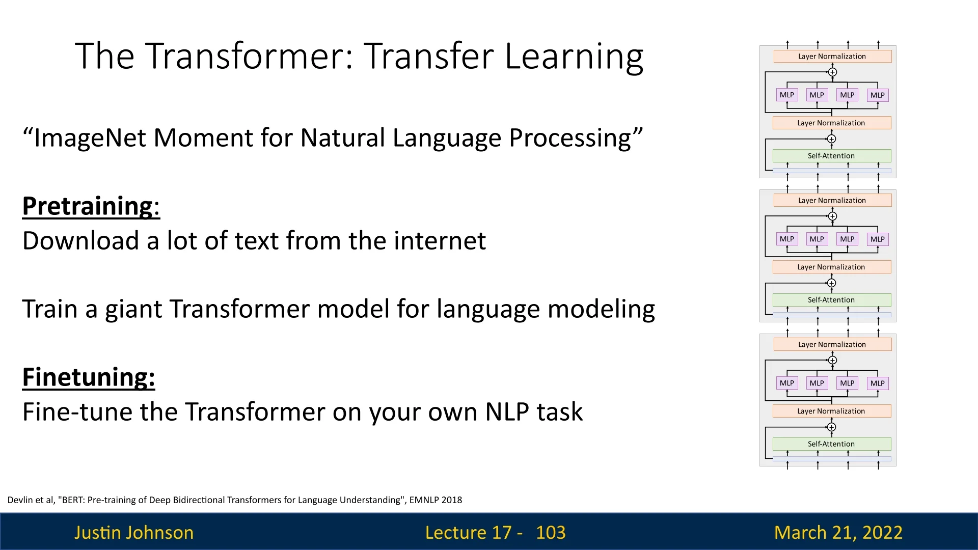
Key benefits of the unified block perspective include:
- Scalability. The separation between attention-based communication and token-wise FFN processing enables efficient GPU utilization in deep stacks.
- Parallelization. Inter-token interaction is confined to self-attention, avoiding the irreducible sequential dependency chain of RNNs.
- Architectural simplicity. For single-stream tasks, a single stack of identical blocks avoids maintaining specialized encoder and decoder implementations.
- Generality at scale. Large decoder-only models demonstrate that the same block family can support a wide range of capabilities with minimal architectural customization.
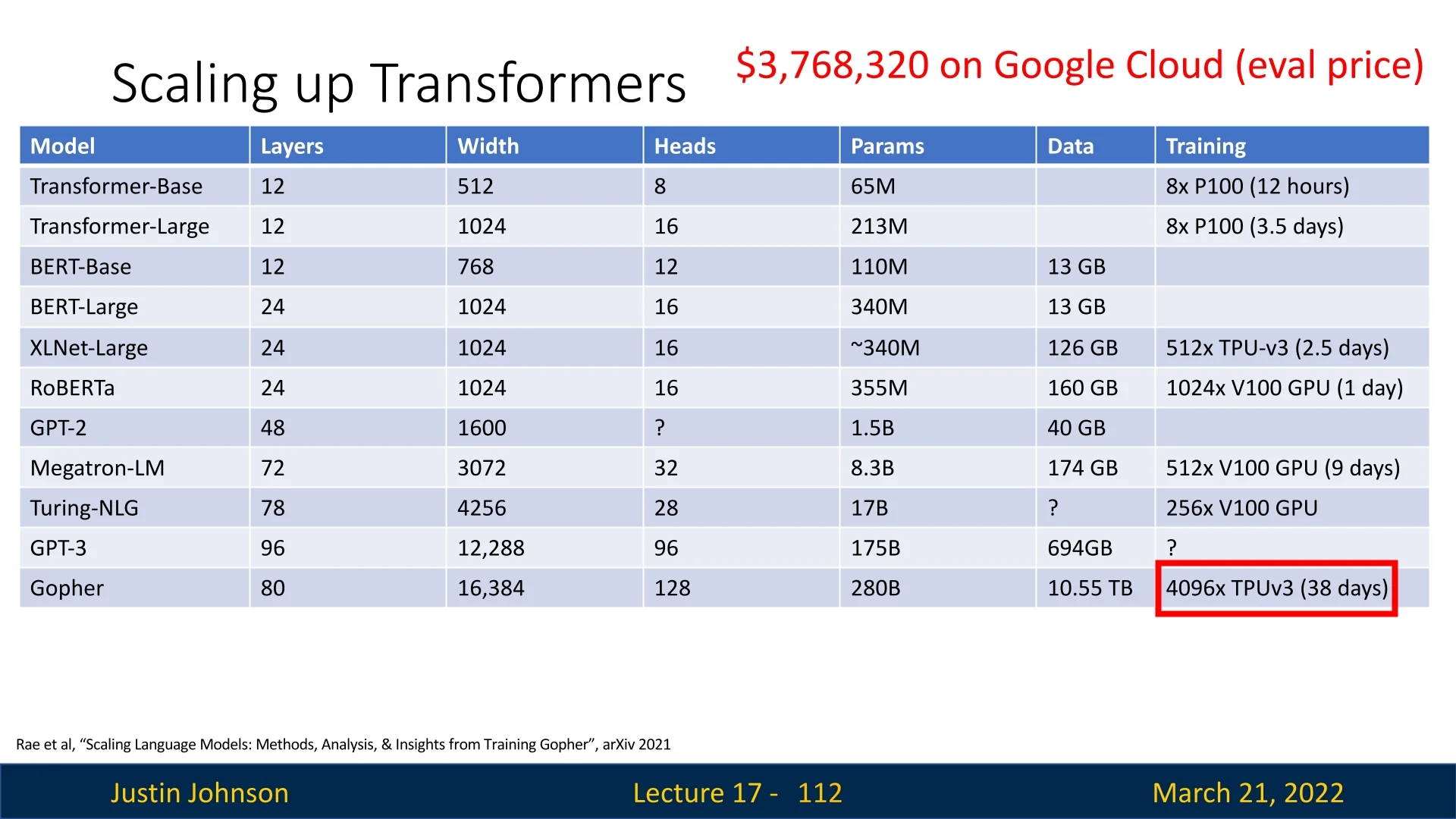
Today’s large-scale models typically adopt this simplified block. As shown in Figure 17.24, newer architectures require substantial computational resources, yet the performance gains have been profound.
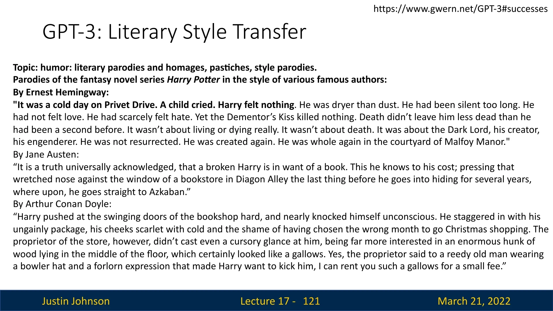
Further Reading and Resources
- The Annotated Transformer: A thorough, annotated PyTorch implementation of the original Transformer from Harvard NLP. It provides step-by-step explanations of each component’s math and code. Available here.
- Transformers from Scratch by Andrej Karpathy: A hands-on video tutorial building a Transformer model in PyTorch from the ground up—ideal for deepening practical understanding. Available here.
Bridging Towards Vision Transformers
Seeing how effectively transformers handle sequences, the next natural step was to apply them to computer vision. Vision Transformers (ViTs) treat image patches as sequences, feeding them through the same self-attention mechanism. This approach now rivals or exceeds state-of-the-art convolution-based methods in image classification, highlighting the remarkable adaptability of the transformer block. In the following chapter, we delve into how images are tokenized and processed through these attention layers, illustrating the expansive reach and potential of transformer-based models.