Lecture 10: Training Neural Networks II
10.1 Learning Rate Schedules
In this lecture, we continue our discussion on training deep neural networks, focusing on strategies to improve optimization efficiency. One of the most critical hyperparameters in training is the learning rate (\(\eta \)). Regardless of the optimizer used—SGD, Momentum, Adagrad, RMSProp, Adam, or others—the learning rate heavily influences training dynamics.
10.1.1 The Importance of Learning Rate Selection
The choice of learning rate significantly impacts the training process:
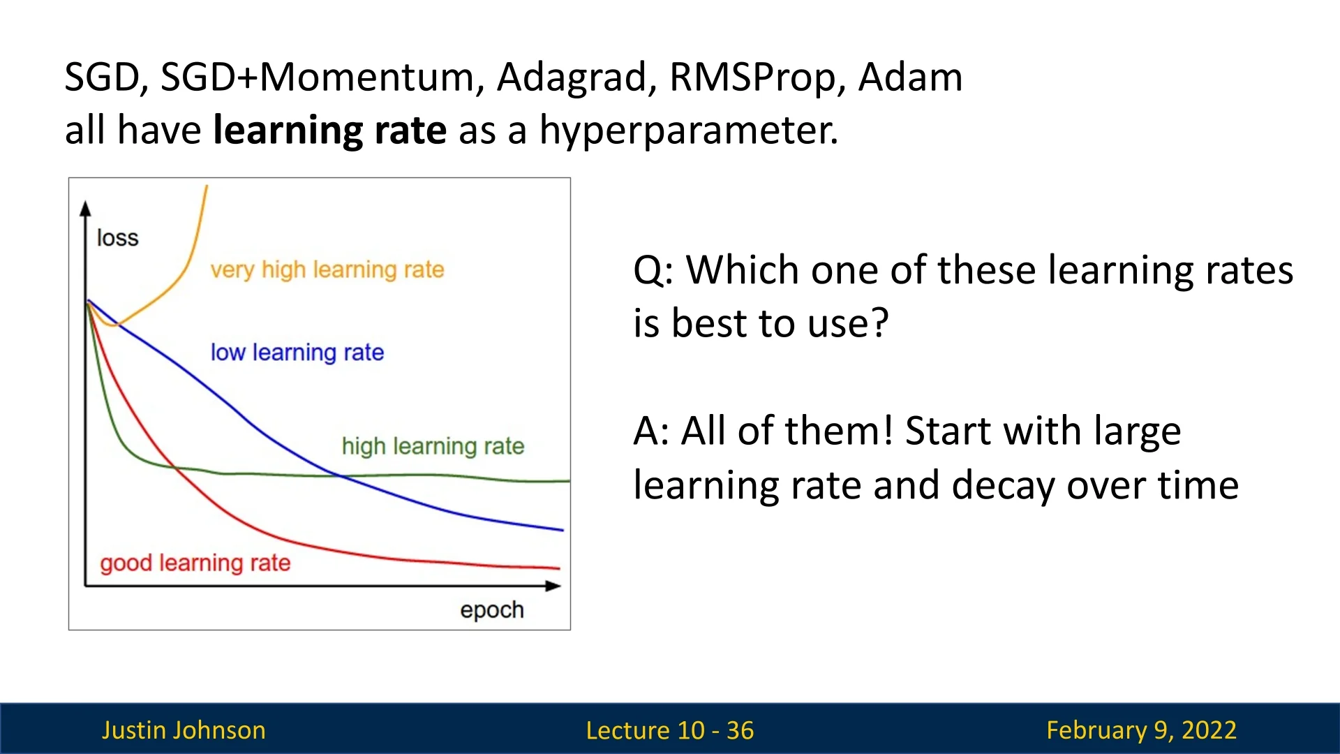
As we can see in the figure 10.1:
- If the learning rate is too high, the training process may become unstable, causing the loss to diverge to infinity or result in NaNs.
- If the learning rate is too low, training will progress extremely slowly, requiring an excessive number of iterations to reach convergence.
- A moderately high learning rate may accelerate training initially but fail to reach the optimal loss value, settling at a suboptimal solution.
- An adequate learning rate achieves a balance between fast convergence and optimal loss minimization.
Since manually choosing an optimal learning rate can be difficult, a common strategy is to start with a relatively large learning rate and decay it over time. This approach combines the benefits of rapid initial learning with stable long-term convergence.
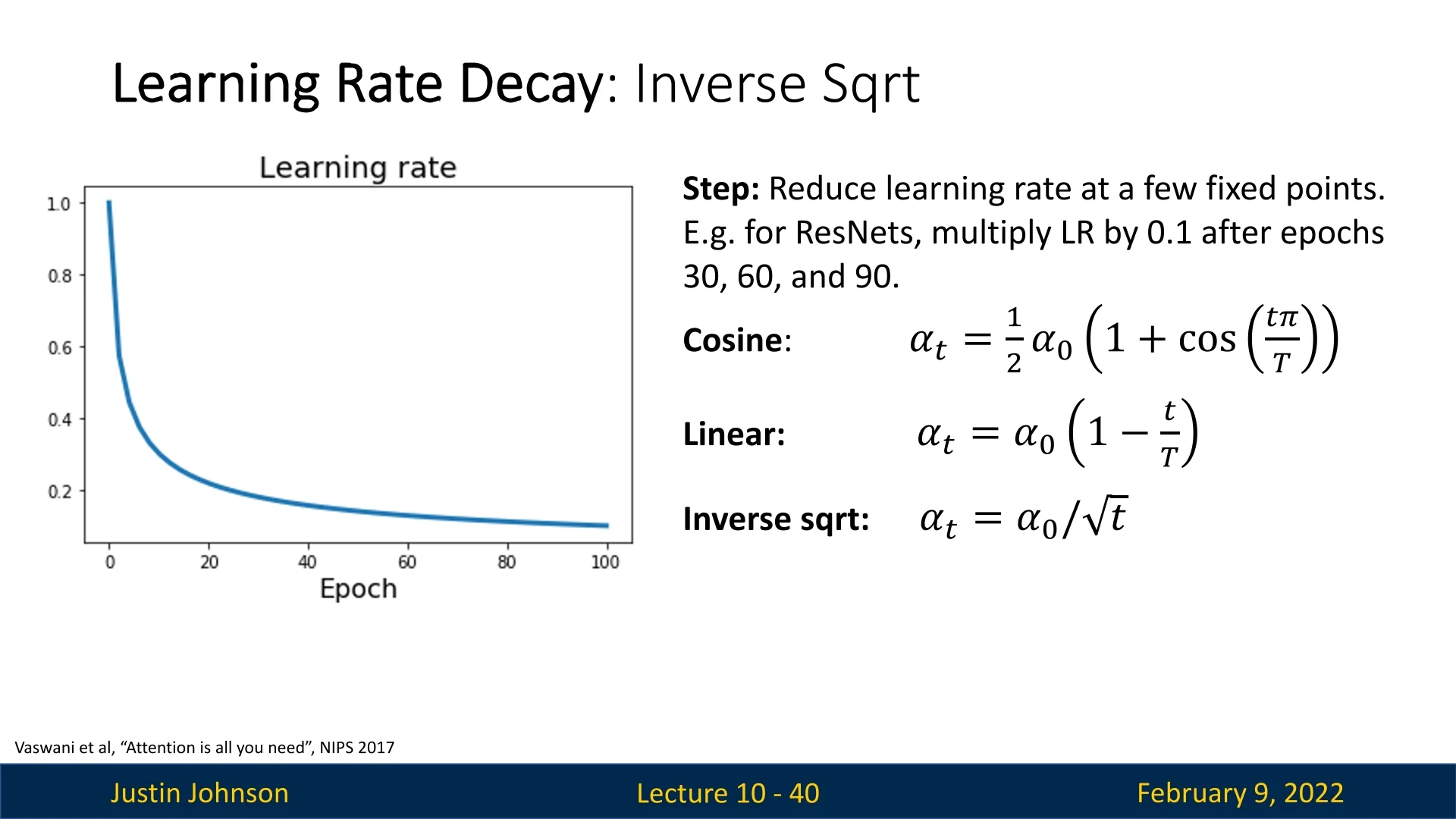
10.1.2 Step Learning Rate Schedule
A widely used method to adjust the learning rate over time is the Step Learning Rate Schedule. This strategy begins with a relatively high learning rate (e.g., \(0.1\) for ResNets) and decreases it at predefined epochs by multiplying it with a fixed factor/factors (e.g., \(0.1\)).
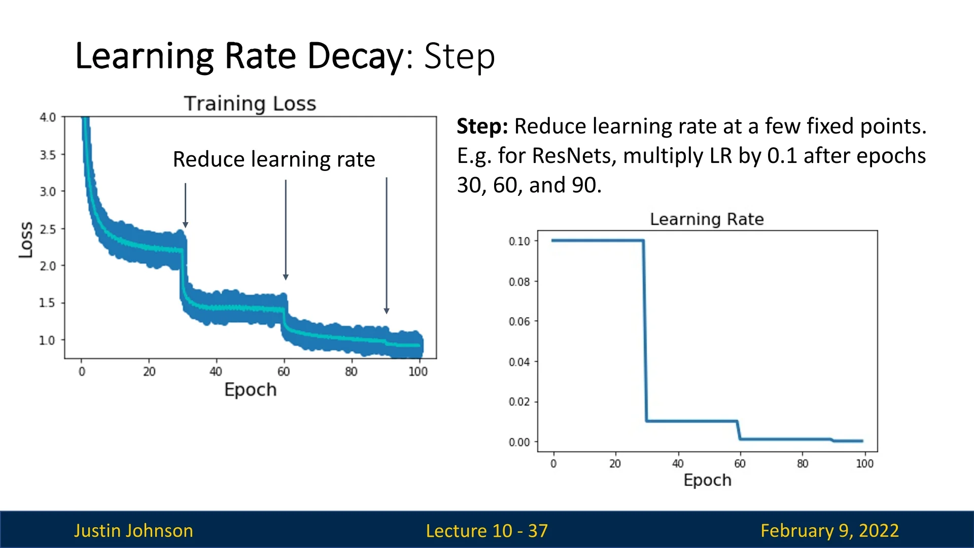
A complete pass through the training dataset is known as an epoch. The Step LR schedule is designed to exploit the exponential loss reduction phase observed in deep learning training. Initially, the loss decreases rapidly, but after a certain number of epochs, progress slows down. At this point, reducing the learning rate initiates a new phase of accelerated loss reduction. In Figure 10.2, we see that lowering the learning rate at epoch 30 causes another rapid improvement, and similar effects occur at epochs 60 and 90.
However, Step LR scheduling introduces several hyperparameters:
- 1.
- Initial learning rate (\(\eta _0\)).
- 2.
- Decay epochs (when to lower the learning rate).
- 3.
- Decay factor (by how much to reduce the learning rate).
These hyperparameters must be tuned manually, often requiring extensive trial and error.
Practical Considerations
One practical approach is to start with a high learning rate, monitor validation accuracy and loss curves, and reduce the learning rate when progress slows down (i.e., when validation accuracy plateaus or loss reduction stagnates). This method allows practitioners to adaptively set the decay points, avoiding the need for fixed schedules.
However, manually adjusting the learning rate can be time-consuming, and automatic methods for adjusting learning rates over time are often preferred. In the following sections, we explore more adaptive learning rate schedules that reduce the need for manual intervention.
10.1.3 Cosine Learning Rate Decay
While the Step LR schedule provides significant improvements over using a constant learning rate, it requires manual selection of multiple hyperparameters. A more automated approach is to use Cosine Learning Rate Decay, which gradually reduces the learning rate in a smooth and continuous manner.
Instead of reducing the learning rate at predefined epochs, as done in step decay, the Cosine Learning Rate Schedule updates the learning rate at each training step.
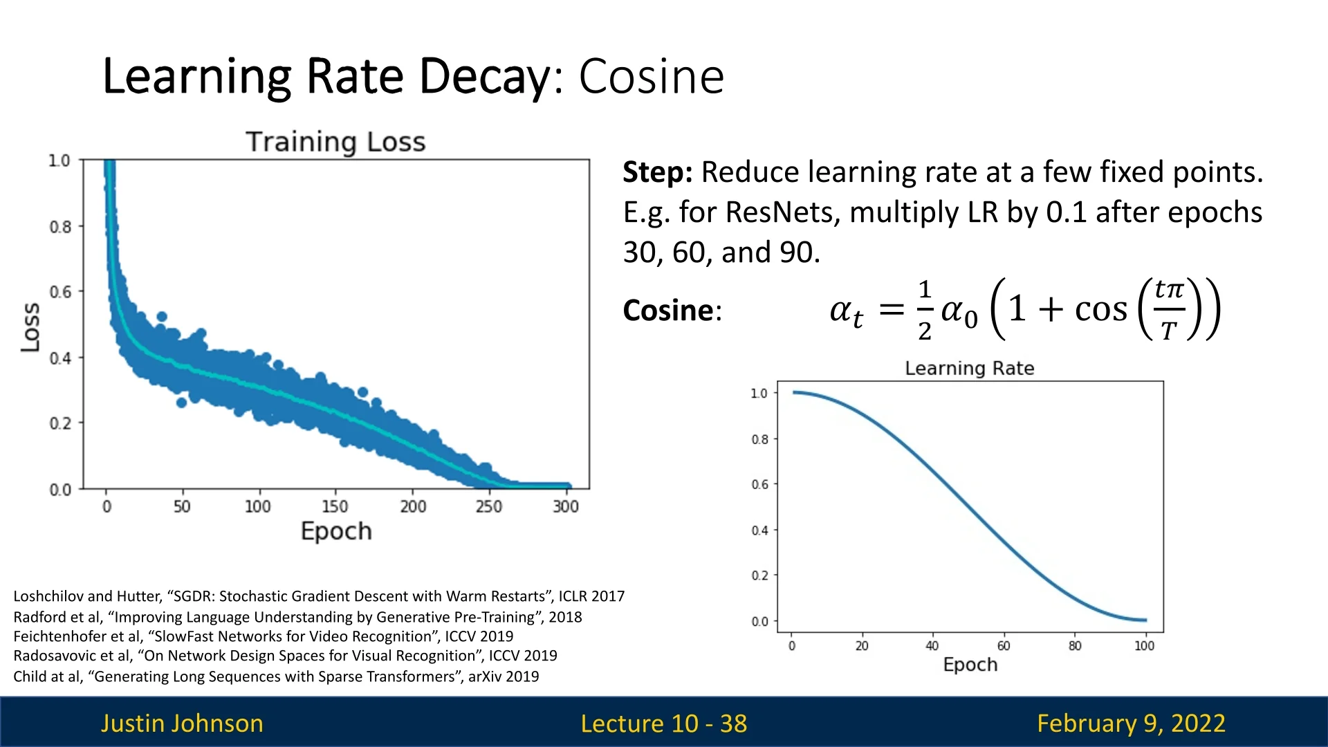
It does so using the following formula: \begin {equation} \alpha _t = \frac {1}{2} \alpha _0 \left (1 + \cos \left ( \frac {t \pi }{T} \right ) \right ), \end {equation}
where:
- \( \alpha _0 \) is the initial learning rate.
- \( t \) is the current epoch.
- \( T \) is the total number of epochs.
This function follows the shape of half a cosine wave, smoothly transitioning from the initial learning rate to near-zero over the course of training.
Advantages of Cosine Decay:
- Only requires two hyperparameters: the initial learning rate \( \alpha _0 \) and the total number of epochs \( T \).
- Both of these parameters are typically chosen in any training setup, making the approach intuitive.
Cosine LR decay has been widely adopted in recent deep learning research, appearing in many high-profile papers at conferences such as ICLR and ICCV.
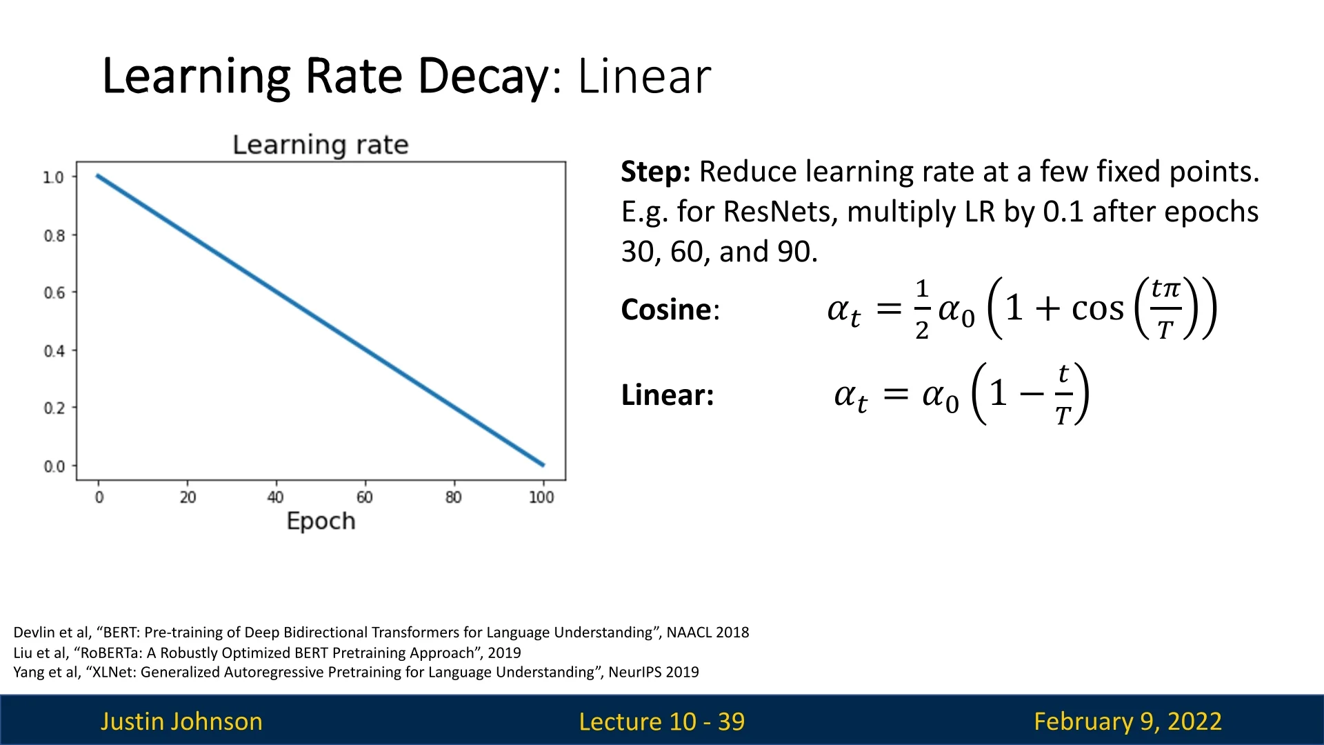
10.1.4 Linear Learning Rate Decay
The cosine decay function is just one possible shape for reducing the learning rate over time. Another simple and effective alternative is Linear Learning Rate Decay, which follows the equation:
\begin {equation} \alpha _t = \alpha _0 \left (1 - \frac {t}{T} \right ). \end {equation}
Here, the learning rate decreases linearly from \( \alpha _0 \) to zero over the training period. It’s important to note that this learning rate schedule is commonly used in the field of NLP, and is less common in popular CV papers. Nevertheless, there is no theoretical ground putting the cosine LR decay a clear winner for the CV research area, and both are applicable.
Comparison Between Cosine and Linear Decay:
- Cosine decay has a more gradual reduction at the beginning and a steeper drop toward the end, which may help with fine-tuning.
- Linear decay provides a consistent reduction rate, which can be beneficial for models that require steady adaptation.
- Both approaches have been used successfully in large-scale models, while the linear decay was even used in previous SOTA models such as BERT [121] and RoBERTa [391].
In many cases, the choice between these schedules is not critical; they are often selected based on conventions within a particular research area rather than empirical/theoretical superiority. The adoption of specific learning rate schedules is often driven by the need for fair comparisons in research rather than their inherent effectiveness.
10.1.5 Inverse Square Root Decay
Another schedule is the Inverse Square Root schedule, where the learning rate at time step \(t\) is defined as: \begin {equation} \alpha _t = \frac {\alpha _0}{\sqrt {t}}. \end {equation} Unlike schedules such as cosine or linear decay, this approach does not require specifying the total number of training epochs (\(T\)). Although less popular, it was notably used in the Transformer model [664], making it a relevant approach to mention.
One drawback of this schedule is its aggressive initial decay. The learning rate decreases rapidly at the beginning of training, meaning the model spends very little time at high learning rates. In contrast, other schedules, such as cosine or linear decay, tend to maintain a higher learning rate for a longer period, which can be beneficial for appropriate training pace.
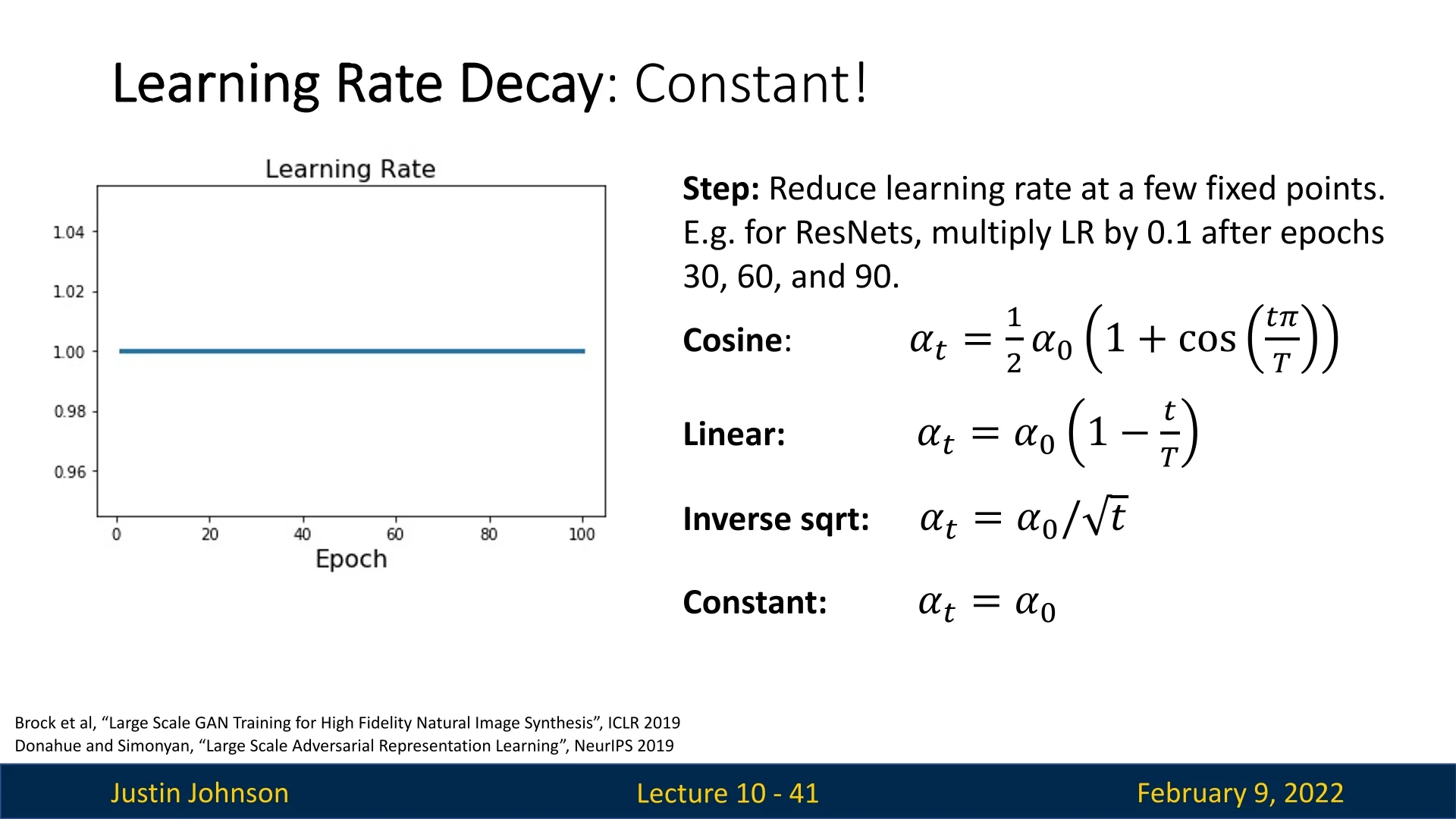
10.1.6 Constant Learning Rate
The last learning rate schedule we present is the constant learning rate, which is the simplest and most common: \begin {equation} \alpha _t = \alpha _0. \end {equation} This schedule maintains a fixed learning rate throughout training. It is often the recommended starting point, as it allows for straightforward debugging and quick experimentation before considering more sophisticated schedules. Adjusting the learning rate schedule should generally be motivated by specific needs, such as:
- Reducing oscillations or instability in training.
- Ensuring convergence towards an optimal solution without premature stagnation.
- Improving generalization performance by fine-tuning decay behaviors.
Although more advanced schedules may improve final performance by a few percentage points, they typically do not turn a failing training process into a successful one. Thus, constant learning rates provide a strong baseline for getting models up and running efficiently.
However, the choice of optimizer plays a crucial role in determining the effectiveness of different learning rate schedules. For instance, when using SGD with Momentum, a more complex learning rate decay schedule is often essential. This is because momentum accumulates gradients over time, and if the learning rate is not adjusted appropriately, the optimization process may become unstable or fail to converge efficiently.
On the other hand, adaptive optimizers such as RMSProp and Adam dynamically adjust learning rates per parameter based on past gradients. This self-adjusting nature allows these optimizers to perform well even with a constant learning rate, as they inherently account for gradient magnitudes and adapt learning rates accordingly.
10.1.7 Adaptive Learning Rate Mechanisms
Adaptive learning rate algorithms such as AdaGrad, RMSProp, and Adam attempt to improve optimization stability by adjusting the learning rate based on gradient statistics. However, relying purely on adaptive mechanisms introduces challenges. A common question is: why not create a mechanism that follows the training loss and adjusts the learning rate accordingly?
The main difficulty in implementing such an approach is the presence of numerous edge cases, such as:
- Noisy loss curves: Training loss fluctuates due to mini-batch noise, making it difficult to extract meaningful trends.
- Slow convergence: Decaying too early or too aggressively can lead to suboptimal solutions.
Despite these challenges, adaptive learning rate techniques remain an essential tool in deep learning optimization, particularly for scenarios involving complex architectures and non-stationary data distributions, in which they tend to shine and provide top-notch results.
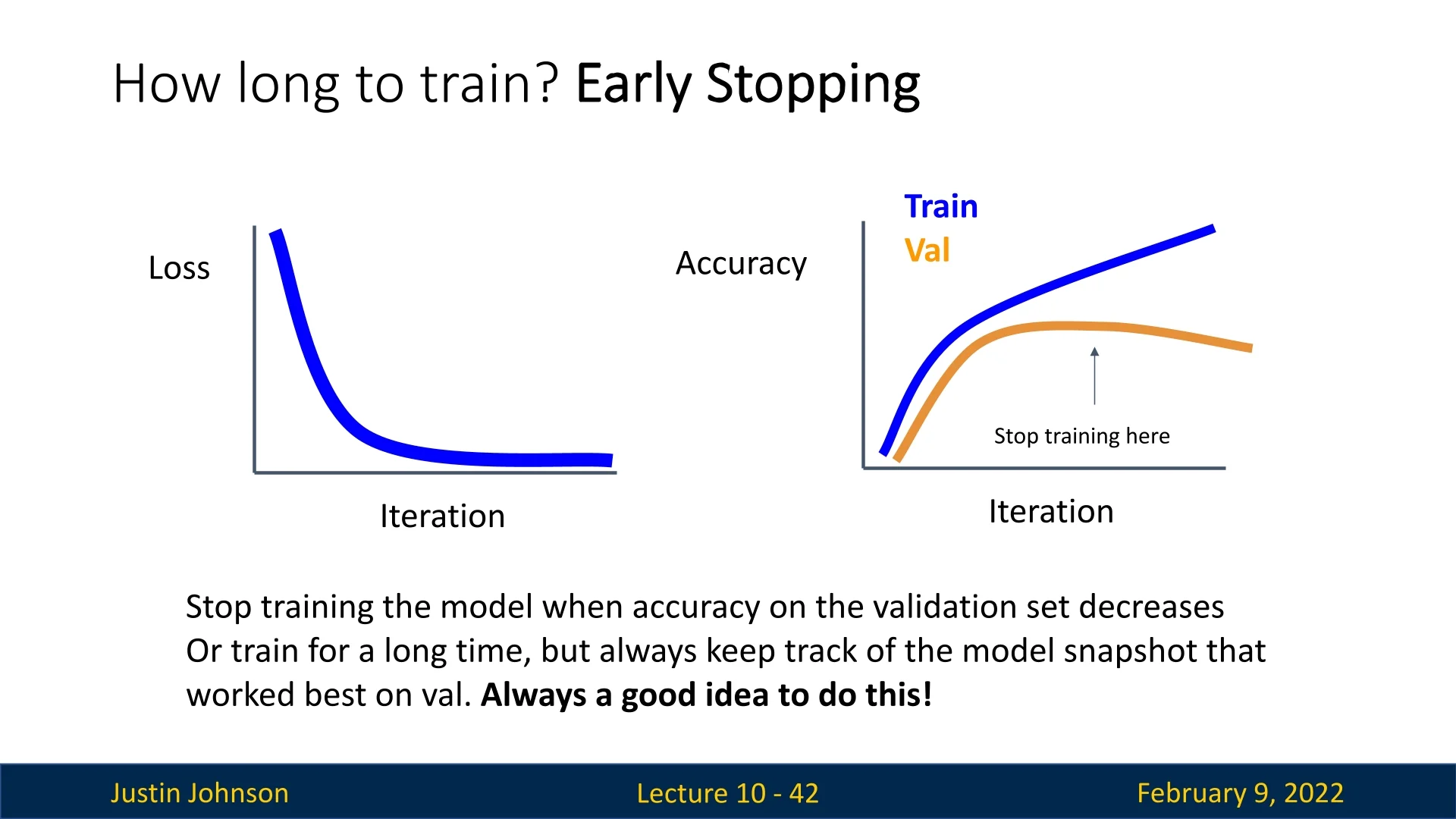
10.1.8 Early Stopping
Another crucial technique to determine when to stop training is early stopping. This method helps prevent overfitting and ensures that the model achieves optimal performance on unseen data. Early stopping relies on monitoring three key curves during training:
- Training loss: This should ideally decay exponentially over time.
- Training accuracy: Should increase steadily as the training loss decreases, indicating that the model is learning effectively.
- Validation accuracy: Should also improve, mirroring the decrease in validation loss.
The idea is to select the checkpoint where the model achieves the highest validation accuracy. During training, model parameters are periodically saved to disk. After training concludes, these checkpoints are analyzed, and the optimal one is chosen based on validation performance. This technique is an effective safeguard against overfitting.
Enrichment 10.1.9: Super-Convergence and OneCycle
Motivation Section 10.1 reviewed monotone learning-rate (LR) schedules—step (subsection 10.1.2), cosine (subsection 10.1.3), linear (subsection 10.1.4), inverse-square-root (subsection 10.1.5)—plus a constant baseline (subsection 10.1.6). These steadily decrease LR to stabilize convergence, but they often under-explore early and require hand-tuned drop epochs. OneCycle [595, 596] flips the pattern: it briefly increases LR to a large peak, then anneals for the remainder of training, while momentum varies inversely. The short high-LR burst adds beneficial stochastic regularization (escaping sharp minima); the long decay polishes in flat regions—often reaching top accuracy in roughly \(1/3\)–\(1/10\) of the epochs of conventional schedules.
Method: schedule and inverse momentum coupling
What we are scheduling (symbols at a glance) At each optimizer update \(t\) (\(t=0,1,\dots ,T\); \(T\) is the total number of updates in the cycle) we control:
- Learning rate \(\boldsymbol {\eta _t}\) (step size at update \(t\)), bounded by three anchors: start \(\eta _{\mbox{min}}\), peak \(\eta _{\mbox{max}}\) (chosen via the LR-range test; see below figure), and end \(\eta _{\mbox{final}}\) (very small, for fine polishing).
- Momentum \(\boldsymbol {m_t}\) (inertia/averaging).1 We bound it between \(m_{\mbox{min}}\) and \(m_{\mbox{max}}\) and couple it inversely to LR (low \(m_t\) when LR is high; high \(m_t\) when LR is low).
A single scalar peak fraction \(p\in (0,1)\) allocates time: the first \(pT\) updates rise to \(\eta _{\mbox{max}}\) (exploration), the remaining \((1-p)T\) decay to \(\eta _{\mbox{final}}\) (refinement).
Notation and helper ramps (defined before use) We describe each phase on its own local timeline.
- Phase lengths. Warm-up length \(L_1 := pT\); anneal length \(L_2 := (1-p)T\).
- Normalized progress. For any phase of length \(L\), set \(\tau := t/L \in [0,1]\). In Phase 1 we use \(\tau _1 = t/L_1\); in Phase 2 we use \(\tau _2 = (t-pT)/L_2\).
- Cosine building blocks. The half-cosine ramp-up \[ \mathrm {hc}(\tau ) := \frac {1-\cos (\pi \tau )}{2} \] smoothly maps \(0\mapsto 0\) and \(1\mapsto 1\) with zero slope at both ends. Its ramp-down companion is \[ \overline {\mathrm {hc}}(\tau ) := 1-\mathrm {hc}(\tau ) = \frac {1+\cos (\pi \tau )}{2}, \] which maps \(0\mapsto 1\) and \(1\mapsto 0\). Any bounds \(a\to b\) are obtained by \(a+(b-a)\,\mathrm {hc}(\tau )\) (up) or \(a+(b-a)\,\overline {\mathrm {hc}}(\tau )\) (down).
Why this shape? (intuition) Monotone decays excel at refinement but can miss broad basins. OneCycle budgets for both: a short, high-LR exploration to inject noise and cross sharp valleys, then a long, low-LR refinement to settle. Stability comes from inverse momentum: near the LR peak we lower momentum (less inertia during big steps); in the tail we raise it (more damping during tiny steps) [595, 596]. Cosine ramps give smooth, zero-slope transitions (no kinks or shocks).
Step-by-step construction of the schedules Phase 1 (exploration, \(0\le t\le pT\)). With \(\tau _1=t/L_1\), \[ \eta _t=\eta _{\mbox{min}}+(\eta _{\mbox{max}}-\eta _{\mbox{min}})\,\mathrm {hc}(\tau _1), \qquad m_t=m_{\mbox{max}}-(m_{\mbox{max}}-m_{\mbox{min}})\,\mathrm {hc}(\tau _1). \] Phase 2 (refinement, \(pT< t\le T\)). With \(\tau _2=(t-pT)/L_2\), \[ \eta _t=\eta _{\mbox{final}}+(\eta _{\mbox{max}}-\eta _{\mbox{final}})\,\overline {\mathrm {hc}}(\tau _2), \qquad m_t=m_{\mbox{min}}+(m_{\mbox{max}}-m_{\mbox{min}})\,\mathrm {hc}(\tau _2). \] Putting the two pieces together: \begin {equation} \eta _t= \begin {cases} \displaystyle \eta _{\mbox{min}}+(\eta _{\mbox{max}}-\eta _{\mbox{min}})\;\frac {1-\cos \!\big (\pi \,\tfrac {t}{pT}\big )}{2}, & 0\le t\le pT\\[8pt] \displaystyle \eta _{\mbox{final}}+(\eta _{\mbox{max}}-\eta _{\mbox{final}})\;\frac {1+\cos \!\big (\pi \,\tfrac {t-pT}{(1-p)T}\big )}{2}, & pT< t\le T \end {cases} \label {eq:chapter10_onecycle_lr} \end {equation} \begin {equation} m_t= \begin {cases} \displaystyle m_{\mbox{max}}-(m_{\mbox{max}}-m_{\mbox{min}})\;\frac {1-\cos \!\big (\pi \,\tfrac {t}{pT}\big )}{2}, & 0\le t\le pT\\[8pt] \displaystyle m_{\mbox{min}}+(m_{\mbox{max}}-m_{\mbox{min}})\;\frac {1-\cos \!\big (\pi \,\tfrac {t-pT}{(1-p)T}\big )}{2}, & pT< t\le T \end {cases} \label {eq:chapter10_onecycle_mom} \end {equation}
What this guarantees. We begin at \((\eta _{\mbox{min}},\,m_{\mbox{max}})\), pass the peak at \((\eta _{\mbox{max}},\,m_{\mbox{min}})\) with zero-slope continuity, and finish at \((\eta _{\mbox{final}},\,m_{\mbox{max}})\). Heuristically, the SGD noise scale scales like \(\eta /(1-m)\), so OneCycle makes it large early (explore) and small late (refine).
Parameterization and defaults Choose \(\eta _{\mbox{max}}\) with the LR-range test (Figure 10.8). Set \[ \begin {aligned} \eta _{\mbox{min}} &= \frac {\eta _{\mbox{max}}}{\texttt{div_factor}}, &\quad \texttt{div_factor} &\in [3,10],\\ \eta _{\mbox{final}} &= \frac {\eta _{\mbox{max}}}{\texttt{final_div_factor}},&\quad \texttt{final_div_factor}&\in [10^3,10^4]. \end {aligned} \] Use \(p\in [0.2,0.4]\) (start with \(0.3\)). For SGD or AdamW [404], robust momentum bounds are \(m_{\mbox{max}}\approx 0.95\), \(m_{\mbox{min}}\approx 0.85\).
What each hyper-parameter controls
- \(\eta _{\mbox{max}}\) (peak LR) — Exploration depth. Higher \(\Rightarrow \) bolder, noisier early steps (faster escape; higher spike risk). Lower \(\Rightarrow \) safer but under-explores. Pick just before instability in the range test.
- \(\eta _{\mbox{min}}\) via div_factor — Launch smoothness. Larger divisor (smaller start LR) \(\Rightarrow \) gentler warm-up (useful for small batches/fragile nets). Smaller \(\Rightarrow \) quicker ramp, more early jitter.
- \(\eta _{\mbox{final}}\) via final_div_factor — Endgame precision. Larger divisor (smaller end LR) \(\Rightarrow \) finer polishing, longer tail. Smaller \(\Rightarrow \) finishes sooner, slightly higher floor.
- \(p\) (peak fraction) — Explore vs. refine budget. Larger \(p\) \(\Rightarrow \) more high-LR time (often modest generalization gains; more instability). Smaller \(p\) \(\Rightarrow \) earlier refinement (safer for short/fragile runs).
- \(m_{\mbox{min}}\) (momentum dip) — Peak control. Lowering loosens control at the LR peak (bolder, riskier); raising tightens control (safer, less regularization).
- \(m_{\mbox{max}}\) (late momentum) — Tail damping. Higher smooths the anneal (fewer oscillations, slower response); lower is snappier but jittery.
Diagnostics: the LR range test
Run a short LR range test [595]: increase LR over a few epochs (linearly or exponentially), record validation loss/accuracy versus LR, and read off a usable LR band. Select \(\eta _{\mbox{max}}\) just before divergence or where accuracy peaks; choose \(\eta _{\mbox{min}}\) where the curve first improves meaningfully. This simple diagnostic removes guesswork and enables OneCycle.
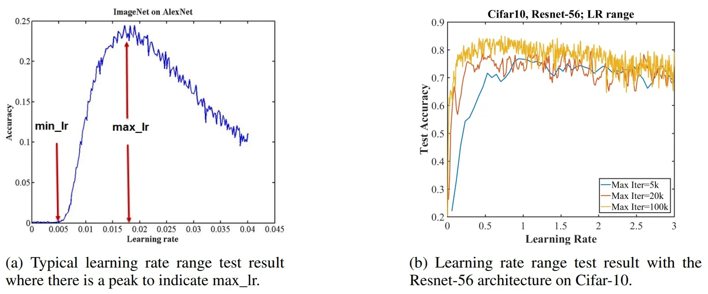
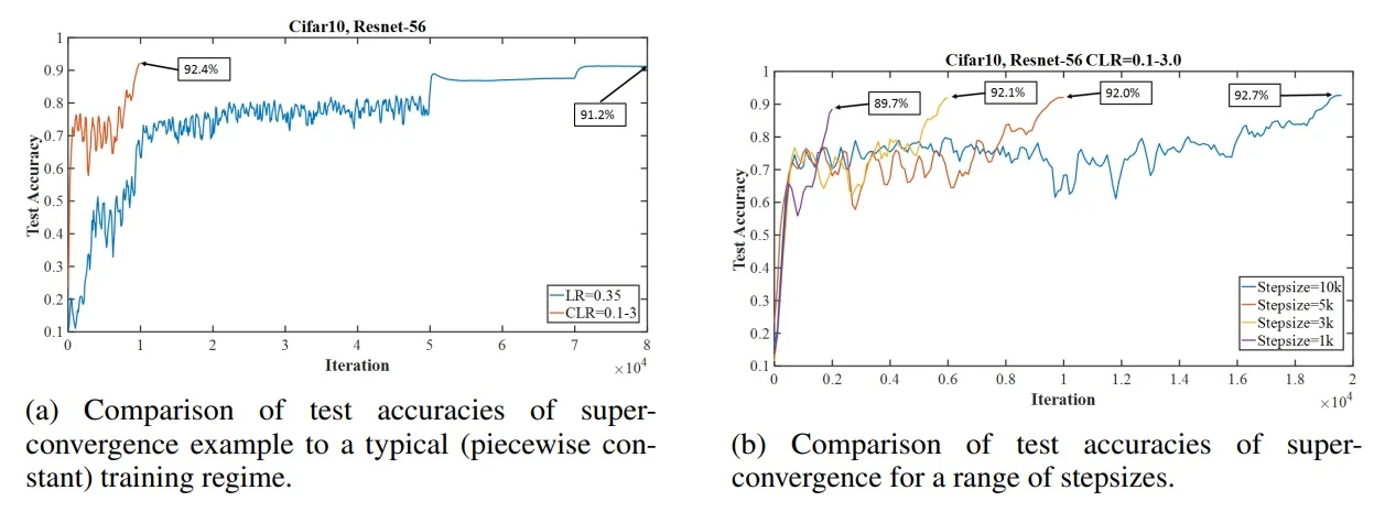
Empirical picture: CIFAR-10 and ImageNet
On CIFAR-10 with ResNet-56, using the LR band in a single-cycle schedule yields pronounced speedups and often higher accuracy. Panel (a) in Figure 10.9 contrasts a typical piecewise-constant baseline (e.g., fixed low LR with scheduled drops) with a OneCycle policy that sweeps between \(\eta _{\mbox{min}}\!\approx \!0.1\) and \(\eta _{\mbox{max}}\!\approx \!3.0\), reaching higher accuracy in far fewer iterations; panel (b) shows that longer cycles (larger stepsize) generally improve final generalization by allowing broader exploration before refinement.
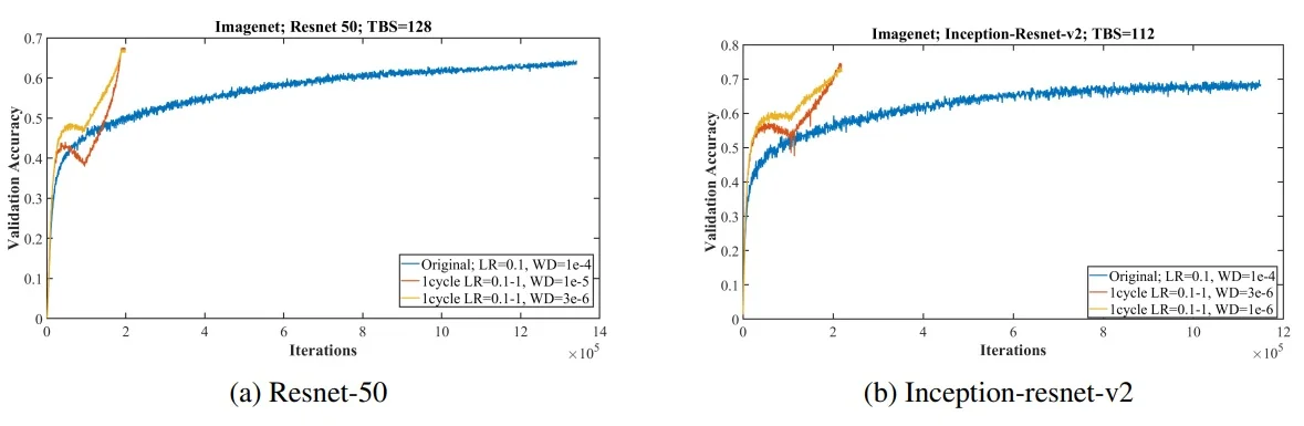
These dynamics scale to ImageNet. Figure 10.10 compares standard training (blue) to a 1cycle policy that displays super-convergence (red/yellow), illustrating that modern backbones (ResNet-50, Inception-ResNet-v2) can train much faster—on the order of \(\sim 20\) versus \(\sim 100\) epochs in representative setups—without loss in final accuracy.
Intuition and comparisons
Big picture. OneCycle makes the exploration–exploitation trade-off explicit: a short high–learning-rate (LR) burst to search broadly, followed by a long low-LR anneal to refine. Momentum is coupled inversely to LR (small \(m_t\) when \(\eta _t\) is large; large \(m_t\) when \(\eta _t\) is small) so the optimizer is agile during exploration and well-damped during refinement. Heuristically, the effective SGD noise scale grows like \(\eta /(1-m)\); OneCycle deliberately makes this large early (regularization, basin jumping) and small late (precision).
How it differs from the schedules in § 10.1—and what this means in practice.
- Versus step decay (subsection 10.1.2). Difference: step uses abrupt, hand-chosen drops; OneCycle is a single smooth rise–then–fall. Practice: fewer plateaus and less guesswork about “drop epochs”, typically faster time-to-target accuracy when drops are not perfectly tuned. Try: if migrating from step, pick \(p\!\approx \!0.3\); if keeping step, place the largest drop near \(t\!\approx \!pT\) to mimic the OneCycle peak.
- Versus cosine decay (subsection 10.1.3). Difference: cosine is smooth but strictly monotone; OneCycle inserts a deliberate LR rise before a cosine-like tail. Practice: the rise acts as a stronger regularizer, often reaching flatter minima sooner at the same epoch budget. Try: start from your cosine baseline, switch to OneCycle with \(\eta _{\max }\) from the range test and \(p\!\in [0.2,0.3]\); add a very short warm-up if needed.
- Versus linear decay (subsection 10.1.4). Difference: linear steadily shrinks LR from the start; OneCycle allocates a fixed high-LR window of length \(pT\) before decay. Practice: linear under-spends time at large LR; OneCycle front-loads exploration then refines. Try: inject a brief rise (\(p\!\approx \!0.2\)) or switch fully to OneCycle to reduce time-to-quality.
- Versus inverse-square-root (subsection 10.1.5). Difference: \(1/\sqrt {t}\) drops quickly early, limiting time at high LR; OneCycle schedules that exploration window (e.g., \(p\!\approx \!0.3\)) and then decays more aggressively to a tiny \(\eta _{\mbox{final}}\). Practice: inverse–sqrt is a safe long-run default for transformers; OneCycle can still help if you cap \(\eta _{\max }\) and keep \(p\) small. Try: for attention-heavy models, use smaller \(\eta _{\max }\) and \(p{=}0.2\); add a very short pre-warm-up if needed.
- Versus constant LR (subsection 10.1.6). Difference: constant LR is flat and simple; OneCycle adds a peak and a long anneal using four anchors \((\eta _{\min },\eta _{\max },\eta _{\mbox{final}},p)\). Practice: constants are great for debugging but need manual decay/early-stopping; OneCycle bakes in exploration and finishing polish, usually reaching equal or better accuracy in fewer epochs. Try: after a range test, set the three LRs via divisors and choose \(p\).
- With adaptive optimizers / large models (subsection 10.1.7). Difference: OneCycle inverts momentum relative to LR (for AdamW, interpret \(m_t\) as \(\beta _1(t)\)) to stabilize the LR peak and damp the tail. Practice: works well with SGD+momentum and AdamW; attention layers and BN statistics are typical sensitivity points near \(\eta _{\max }\). Try: cap \(\eta _{\max }\) lower than your CNN default, set \(p\!\approx \!0.2\), and consider a very short warm-up; if you see peak-time spikes, reduce \(\eta _{\max }\), increase \(m_{\min }\) slightly, or shorten \(p\).
When to use—and caveats
Where it shines. Use OneCycle when
- Compute / epochs are limited: you need near-peak accuracy in fewer epochs or shorter wall-clock than step/cosine baselines.
- You want a strong baseline quickly: only the LR-range test is required to set \(\eta _{\max }\); the rest follows from simple divisors and a single \(p\) (subsubsection 10.1.9.0).
- Standard supervised setups: CNNs and transformers trained with SGD + momentum or AdamW on mid/large datasets, where an early regularization pulse and a long anneal are beneficial.
- You can run an LR-range test: selecting \(\eta _{\max }\) empirically is part of the method.
Gray areas—use with care (why, and what to try).
- Very small or very noisy datasets. Why: the LR peak can over-regularize or destabilize. Try: reduce \(\eta _{\max }\) by \(20\)–\(50\%\); use \(p{=}0.2\); or switch to cosine with a brief warm-up.
- Attention-heavy models (ViTs/LLMs). Why: large LR can perturb attention/normalization scales. Try: cap \(\eta _{\max }\) below your CNN default; set \(p{=}0.2\); optionally add a short pre–warm-up (few hundred steps); raise \(m_{\min }\) slightly for more control.
- Strong regularization stacks (heavy aug + large WD). Why: the peak adds noise on top of existing regularizers, risking underfit. Try: keep WD fixed and lower \(\eta _{\max }\); extend \(p\) only if training loss remains smooth; prefer the cosine tail.
- Tight gradient clipping or tiny microbatches. Why: small clip norms nullify the intended large steps at the peak. Try: relax clipping (e.g., clip \(\approx 1\)) or lower \(\eta _{\max }\); otherwise use a monotone cosine schedule.
- BatchNorm drift near the peak. Why: high LR perturbs running means/variances. Try: reduce \(\eta _{\max }\); increase \(m_{\min }\) by \(0.02\)–\(0.05\); shorten \(p\); consider freezing BN stats for a short window around the peak if absolutely necessary.
Generally not a win (prefer other schedules).
- Already well-tuned long cosine. If your baseline already uses a long, smooth anneal with strong results, OneCycle’s gains may be marginal. Alternative: keep cosine or inject a very short initial ramp (small \(p\)) for a modest speedup.
- No LR-range test possible. If you cannot estimate \(\eta _{\max }\) (e.g., streaming/online constraints), prefer a conservative cosine with warm-up.
- Extremely short runs. If \(pT\) would be only a handful of steps, the peak is poorly resolved. Alternative: use warm-up \(\rightarrow \) cosine or linear decay.
Rule of thumb. If uncertain, start with the recipe in subsubsection 10.1.9.0: range-test \(\eta _{\max }\), set \(\eta _{\min }\) and \(\eta _{\mbox{final}}\) by divisors, choose \(p{=}0.3\), and adjust only when you observe peak-time spikes (lower \(\eta _{\max }\) / raise \(m_{\min }\) / shorten \(p\)) or late plateaus (smaller \(\eta _{\mbox{final}}\) via larger final_div_factor).
- 1.
- Pick the LR band (required). Run the LR-range test; set \(\eta _{\max }\) just before instability. Set \(\eta _{\min }=\eta _{\max }/\texttt{div_factor}\) with div_factor\(\in [10,25]\) for stability (use \([3,10]\) if you want a faster launch). Set \(\eta _{\mbox{final}}=\eta _{\max }/\texttt{final_div_factor}\) with final_div_factor\(\in [10^3,10^4]\).
- 2.
- Allocate time. Start with \(p{=}0.3\). If the peak region is spiky, shorten to \(p{=}0.2\); if validation keeps improving with longer exploration, consider \(p{=}0.35\)–\(0.40\).
- 3.
- Stabilize the peak (priority order).
- (a)
- Reduce \(\eta _{\max }\) by \(10\)–\(20\%\).
- (b)
- Increase \(m_{\min }\) by \(0.02\)–\(0.05\) (adds control at the peak).
- (c)
- Increase div_factor (smaller \(\eta _{\min }\) for a gentler launch).
- (d)
- Optionally shorten \(p\) by \(0.05\).
- 4.
- Polish the tail. If the final metric plateaus high, increase final_div_factor (smaller \(\eta _{\mbox{final}}\)). If time-limited, accept a slightly larger \(\eta _{\mbox{final}}\) for a faster finish.
- 5.
- Keep the rest steady. Use decoupled weight decay (AdamW/SGD+WD) held constant; avoid very tight gradient clipping at the peak (clip \(\approx 1\) is a common ceiling). Ensure the scheduler steps once per optimizer update.
- 6.
- Transformer-specific tip. Map \(m_t\) to \(\beta _1(t)\) for AdamW; prefer \(p{=}0.2\) and a slightly smaller \(\eta _{\max }\); add a very short pre-warm-up if attention becomes unstable.
10.2 Hyperparameter Selection
Choosing the right hyperparameters is a crucial step in training deep learning models. In this section, we discuss different strategies for hyperparameter selection and practical methods to make the process efficient.
10.2.1 Grid Search
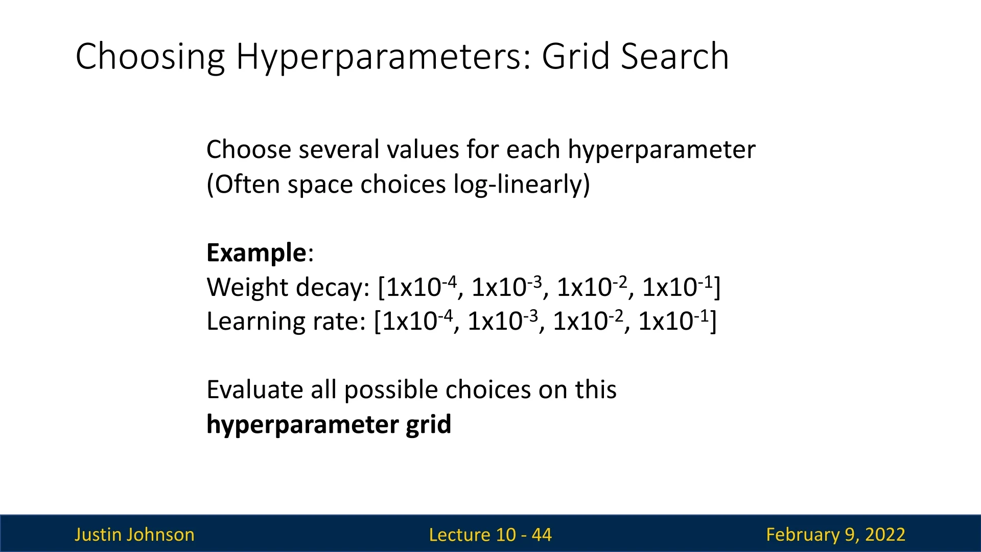
A common approach is grid search, where we define a set of values for each hyperparameter and evaluate all possible combinations. Typically, hyperparameters such as weight decay, learning rate, and dropout probability are spaced log-linearly or linearly, depending on their nature. For example:
- Weight decay: \([10^{-4}, 10^{-3}, 10^{-2}, 10^{-1}]\)
- Learning rate: \([10^{-4}, 10^{-3}, 10^{-2}, 10^{-1}]\)
Given these choices, we have \(4 \times 4 = 16\) configurations to evaluate. If sufficient computational resources are available, all combinations can be tested in parallel. However, as the number of hyperparameters increases, the search space grows exponentially, making grid search infeasible for a large number of parameters.
10.2.2 Random Search
It is counter-intuitive, but empirical evidence suggests that random search often outperforms grid search in most scenarios by reaching better results faster. The study [38] explains why. The key insight is that hyperparameters can be classified into important and unimportant ones:
- Important hyperparameters significantly affect model performance.
- Unimportant hyperparameters have little to no effect.
When we begin training, it is difficult to determine which hyperparameters fall into which category. In grid search, every combination of hyperparameters is systematically evaluated, meaning we sample the important parameters in a structured but inefficient manner.
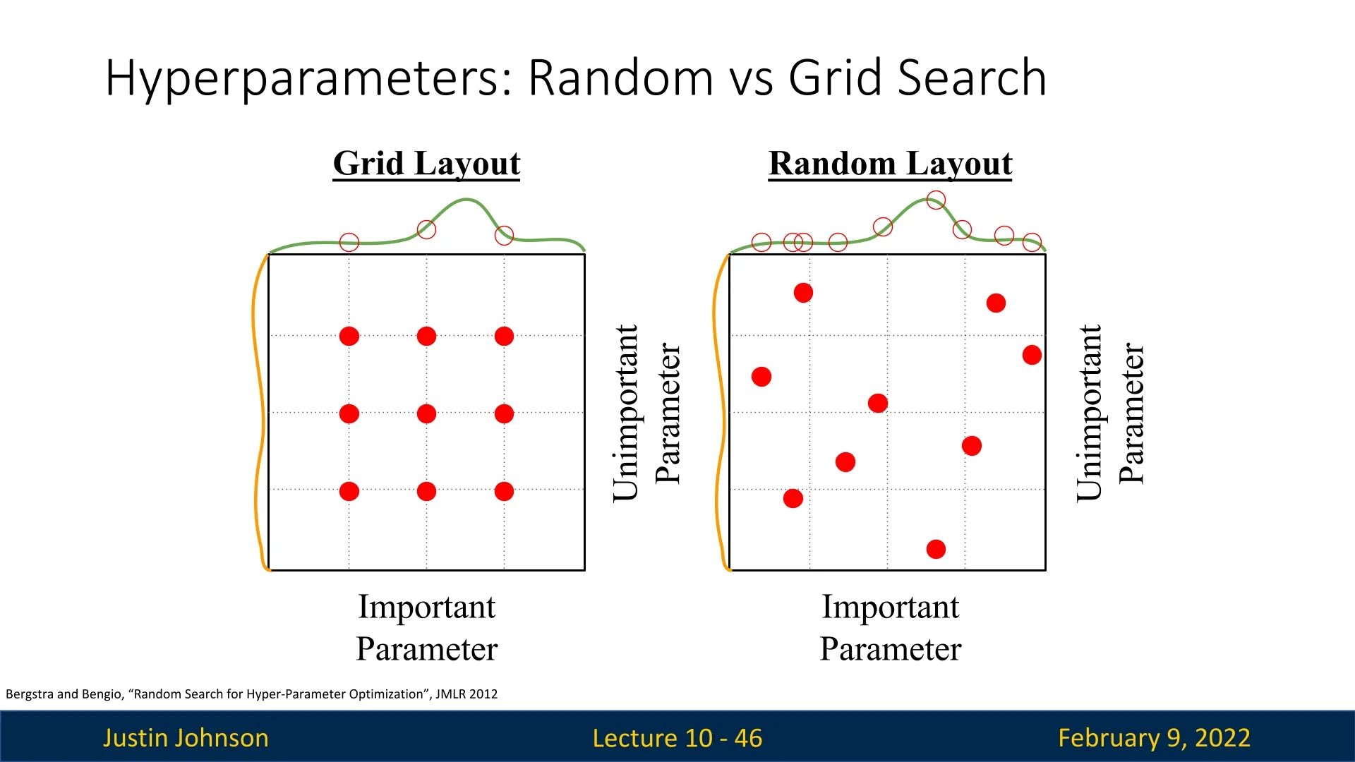
For example, in Figure 10.12, consider a scenario with two hyperparameters:
- The vertical axis (orange distribution) represents an unimportant parameter that does not significantly impact accuracy.
- The horizontal axis (green distribution) represents an important parameter with a small sweet spot near the middle, which yields the best accuracy.
Using grid search, each value of the important hyperparameter is evaluated for all values of the unimportant one. If we have a \(3 \times 3\) grid, we get only three different values for the important parameter, potentially missing the peak of the green distribution. Since grid search samples systematically, many trials will be wasted on evaluating different values of the unimportant parameter without gathering enough information about the critical one.
In contrast, random search selects hyperparameters independently, meaning more trials sample different values of the important parameter. This increases the likelihood of hitting the peak region of the green curve at least once, thereby selecting a better-performing model configuration.
10.2.3 Steps for Hyperparameter Tuning
Hyperparameter tuning is one of the most computationally expensive yet crucial stages in model optimization. When resources are limited, adopting a structured, iterative strategy prevents wasted effort on uninformative configurations. The following process combines diagnostic sanity checks with a principled exploration of the hyperparameter space.
Importantly, while grid search systematically evaluates all parameter combinations, research has shown that random search is typically far more effective in high-dimensional settings [39]. Grid search wastes trials exploring unimportant dimensions uniformly, whereas random sampling explores a wider variety of promising configurations, often finding strong solutions several times faster.
- 1.
- Check the Initial Loss: Sanity Verification
Before extensive training, verify that the model behaves sensibly at initialization. This early diagnostic catches systemic bugs or poor scaling before any tuning begins.- Disable weight decay, dropout, and data augmentation to isolate core dynamics.
- For a softmax classifier with \( C \) classes, the expected initial cross-entropy loss is roughly \( \log C \).
-
Significant deviations usually signal issues such as:
- Mis-scaled input data (e.g., missing normalization).
- Mis-specified loss function or bug in label encoding.
- Improper initialization (e.g., exploding or vanishing activations).
- 2.
- Overfit a Tiny Dataset: Model Capacity Check
Test whether the model can memorize a very small dataset (5–10 minibatches). This step confirms that the model and optimizer can learn under ideal conditions.- Train with all regularization disabled.
- The model should reach near-100% training accuracy quickly.
-
Failure to overfit indicates deeper issues:
- Learning rate too low or initialization too weak.
- Architecture too shallow or underparameterized.
- Data pipeline or loss computation errors.
- 3.
- Find a Viable Learning Rate: Sensitivity Test
Use the full dataset with minimal regularization to determine a good learning rate (LR) range.- Start with a small L2 penalty (e.g., \( 10^{-4} \)).
- Try a logarithmic sweep: \( 10^{-1}, 10^{-2}, 10^{-3}, 10^{-4} \).
- The ideal LR produces a steady, exponential loss decrease in the first 100–200 iterations.
- Too high → divergence or NaNs; too low → stagnant loss.
A good learning rate is the foundation of every successful tuning cycle.
- 4.
- Run a Coarse Random Search: Global Exploration
Instead of testing every grid combination, sample hyperparameters randomly from broad distributions for short runs (e.g., 3–5 epochs each).- Random search covers more unique configurations and avoids wasting trials on irrelevant parameter combinations.
-
Example sampling ranges:
- Learning rate: log-uniform in [\(10^{-4}\), \(10^{-1}\)].
- Weight decay: log-uniform in [\(10^{-6}\), \(10^{-3}\)].
- Dropout: uniform in [0, 0.6].
- Batch size: categorical in {32, 64, 128} (depending on hardware).
- Run 10–20 trials and rank by validation performance.
This step identifies promising regions of the search space without expensive exhaustive evaluation.
- 5.
- Refine the Search: Local Exploitation
Focus the next round of random search within narrower ranges around the best-performing configurations.- For example, if good learning rates cluster near \(2 \times 10^{-3}\), search between \(10^{-3}\) and \(5 \times 10^{-3}\).
- Gradually add regularization (dropout, weight decay) or data augmentation if overfitting appears.
- Train longer (10–30 epochs) to evaluate generalization more accurately.
This step transitions from exploration to fine-tuning, exploiting the discovered “sweet spot.”
- 6.
- Analyze Learning Curves: Interpret Behavior
Plot and inspect training/validation loss and accuracy to understand optimization dynamics.- Validation loss decreasing → under-training; train longer.
- Large train–val gap → overfitting; increase regularization.
- Both high and flat → underfitting; try a larger model or higher LR.
Quantitative metrics are essential, but qualitative curve inspection often reveals misconfigurations faster than automated heuristics.
- 7.
- Iterate and Converge: Continuous Refinement
Hyperparameter tuning is inherently iterative. Use results from Step 6 to guide further random sampling or to introduce advanced techniques:- Apply learning rate schedules (e.g., cosine decay, OneCycle).
- Use early stopping to save compute on poor configurations.
- Combine the top 3–5 tuned models in an ensemble for improved robustness.
Continue refining until performance saturates or computational limits are reached.
This structured pipeline—diagnose, sanity-check, explore broadly via random sampling, then refine and interpret—turns hyperparameter tuning from blind trial-and-error into an informed, iterative optimization process. In practice, random search achieves competitive results with an order of magnitude fewer trials than grid search, especially when parameters interact nonlinearly.
10.2.4 Interpreting Learning Curves
Analyzing learning curves provides valuable insights into model performance. Some common learning curve patterns and their implications are:
-
Very Flat at the Beginning, Then a Sharp Drop: This typically indicates poor initialization, as the model fails to make enough progress at the start of training.
- A likely solution is to reinitialize the weights using a more suitable initialization method (e.g., Xavier or He initialization).
- If the loss remains stagnant, check if the learning rate is too low.
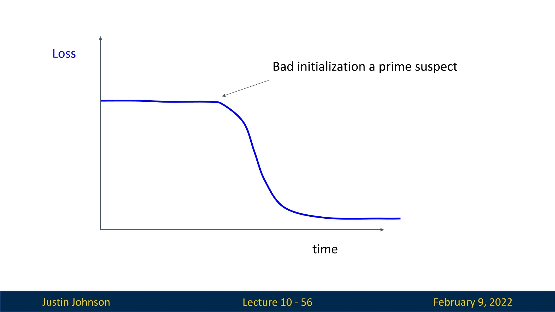
Figure 10.13: A learning curve that is very flat at the beginning and then drops sharply, indicating poor initialization. -
Plateau After Initial Progress: If the loss decreases at first but then flattens out, the model may have reached a suboptimal local minimum.
- Introducing learning rate decay (e.g., step decay, cosine decay, or inverse square root decay) at the right point can help the model escape the plateau.
- Increasing model complexity (e.g., adding more layers or neurons) might be necessary.
- Increasing weight decay or using a more sophisticated optimization method could be useful if we are stuck in this state.
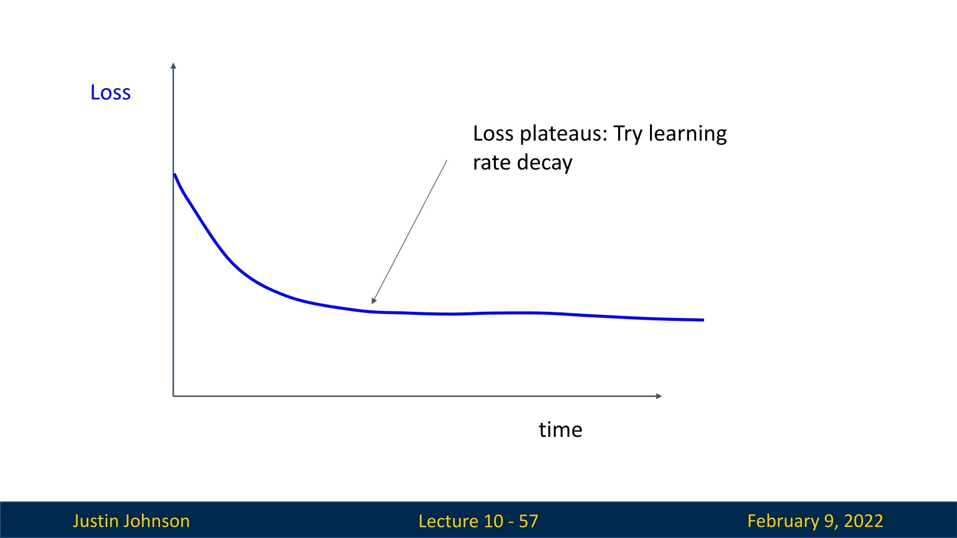
Figure 10.14: Learning curve plateauing, indicating the need for learning rate decay or weight decay tuning. -
Step Decay Causing Stagnation: If a sharp drop in the learning rate is applied too early, the loss may stop improving.
- The learning rate should ideally be reduced gradually rather than abruptly.
- Implementing adaptive decay schedules based on validation loss can prevent premature stagnation.
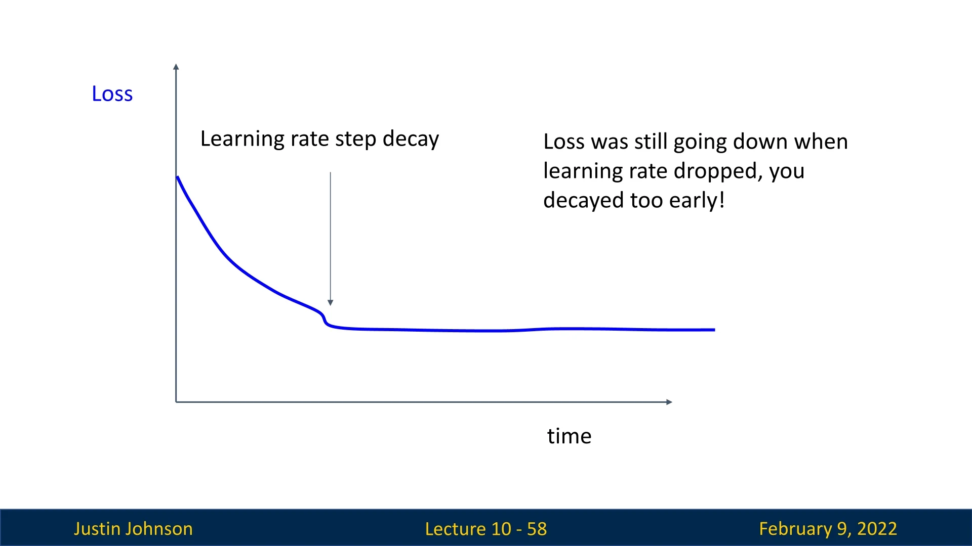
Figure 10.15: Step decay applied too early, leading to stagnation. Adjusting the decay timing may help. -
Continued Accuracy Growth: If both training and validation accuracy continue increasing, training should be extended.
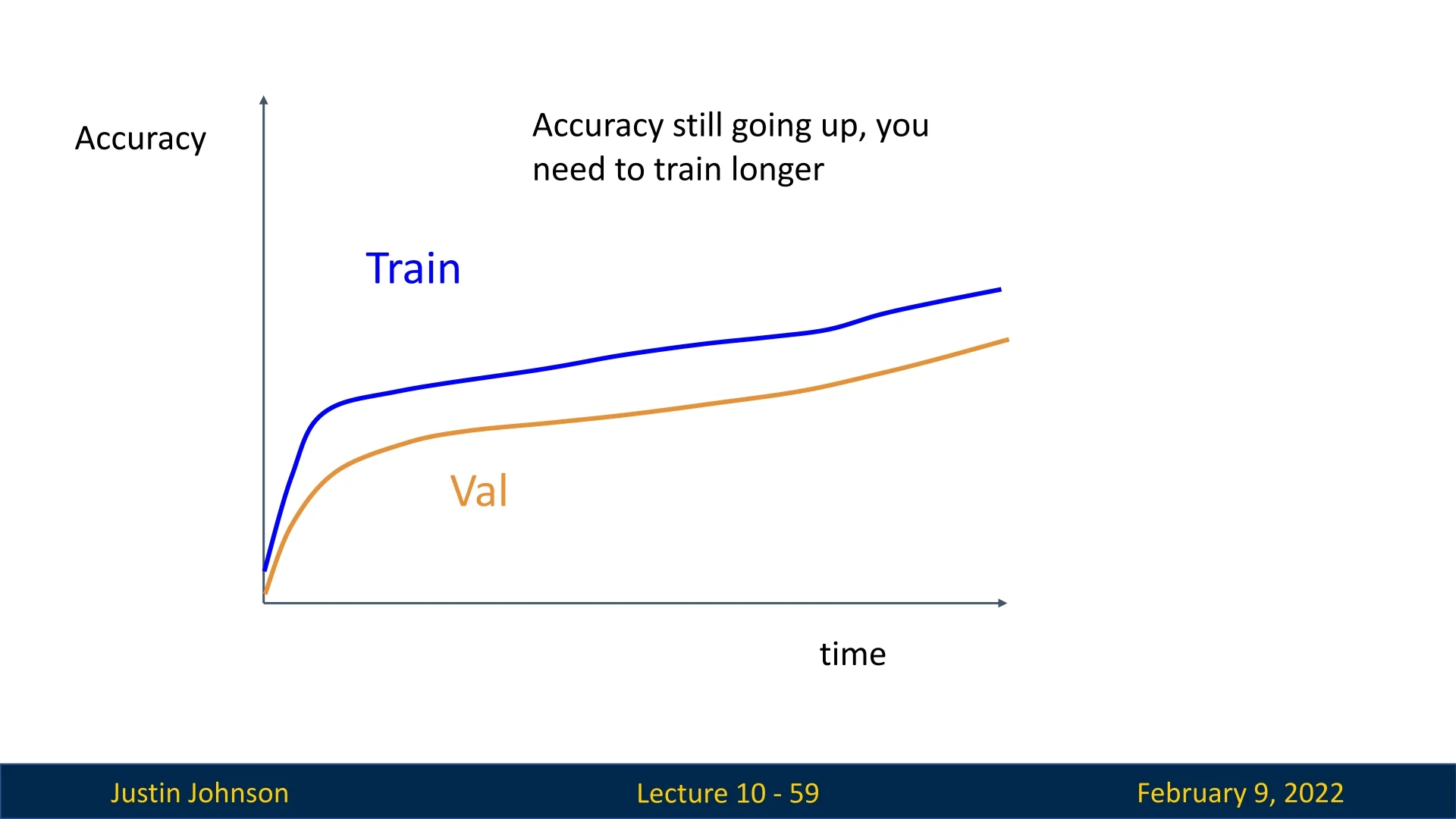
Figure 10.16: Accuracy still increasing, suggesting longer training is needed. -
Large Train-Validation Gap (Overfitting): If training accuracy keeps increasing while validation accuracy plateaus or drops, overfitting is likely occurring.
- Solutions include increasing regularization, expanding the dataset, or simplifying the model.
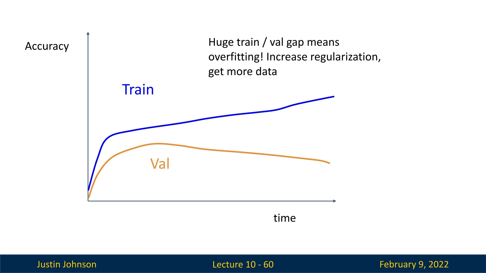
Figure 10.17: Train-validation accuracy gap, indicating overfitting. Regularization techniques may help. -
Train and Validation Accuracy Increasing Together (Underfitting): If both curves are increasing but are gap between the train and val accuracy is much lower than expected, the model might be underfitting.
- Possible solutions include increasing model capacity, training for longer, or reducing excessive regularization.
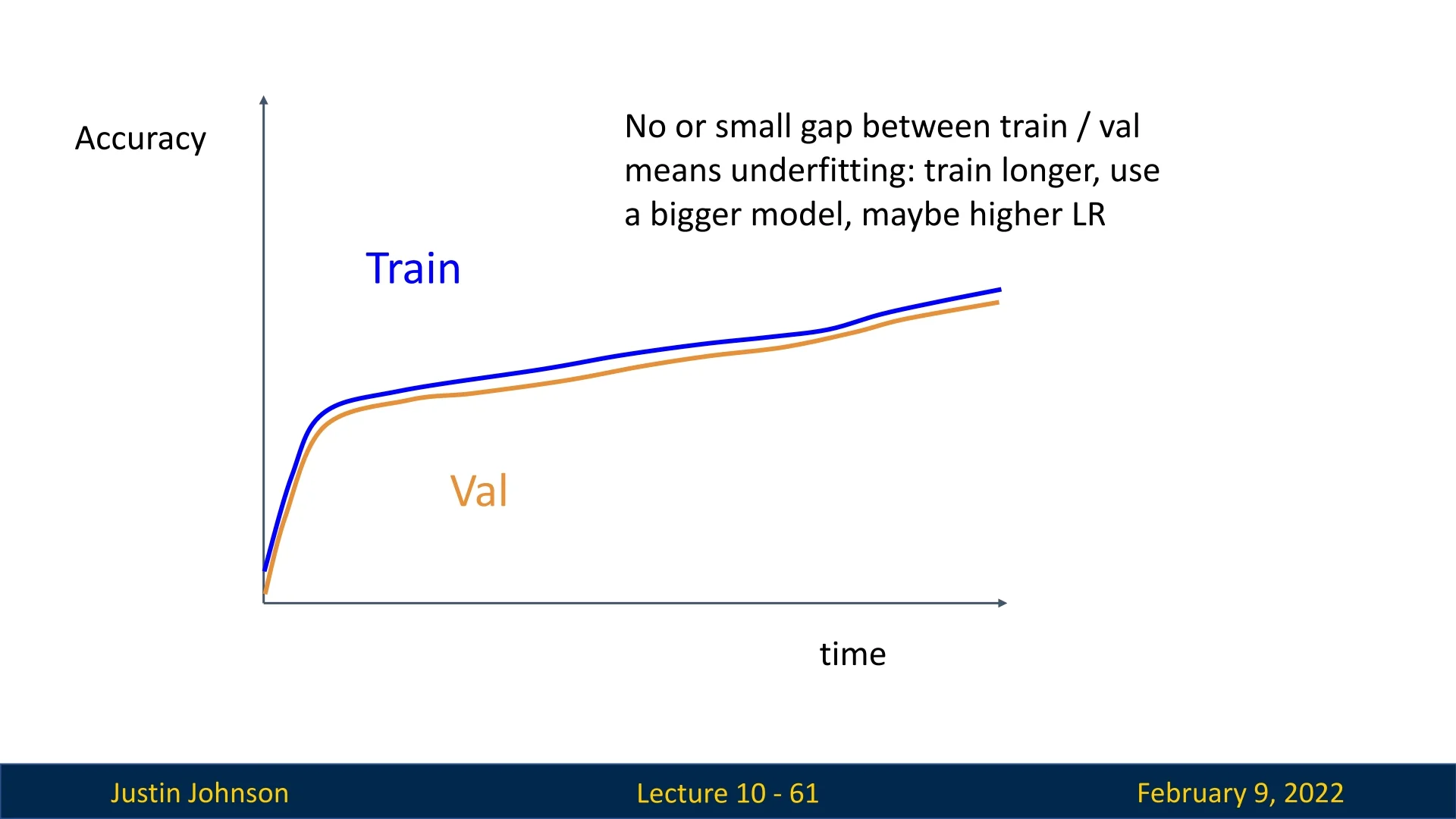
Figure 10.18: Underfitting: train and validation accuracy increasing together but at a low level. Model capacity should be increased.
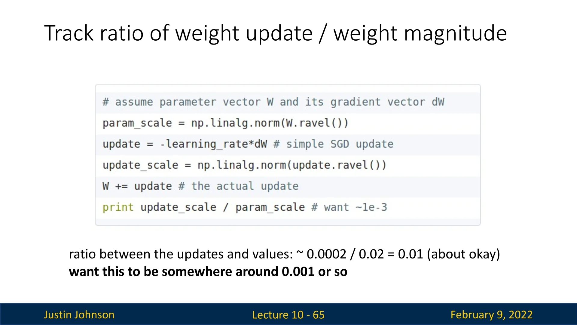
Beyond loss and accuracy curves, tracking the weight update-to-weight magnitude ratio is useful for diagnosing training stability:
- A ratio around 0.001 is typically healthy.
- If the ratio is too high, learning might be unstable.
- If the ratio is too low, learning might be too slow, requiring a learning rate adjustment.
When training multiple models in parallel or sequentially (as seen in Step 6), analyzing different learning curves helps guide further hyperparameter adjustments. Prior to modern visualization tools like TensorBoard, interpreting learning progress was challenging. Today, tools such as Wandb, MLflow, and Comet enable real-time logging and comparison of models, making hyperparameter tuning more efficient. By leveraging these insights, we can iteratively refine our model selection process and improve generalization to unseen data.
10.2.5 Model Ensembles and Averaging Techniques
Model ensembling is a widely used technique that can provide an additional 1-2% performance boost compared to using a single model, regardless of architecture, dataset, or task. The core idea is to train multiple independent models and, at test time, aggregate their outputs to achieve better generalization and robustness.
For classification tasks, an effective ensembling method is to average the probability distributions predicted by different models and then select the class with the highest average probability: \begin {equation} \hat {y} = \arg \max \frac {1}{N} \sum _{i=1}^{N} P_i(y | x) \end {equation} where \(N\) is the number of models in the ensemble, and \(P_i(y | x)\) is the probability distribution predicted by the \(i\)-th model.
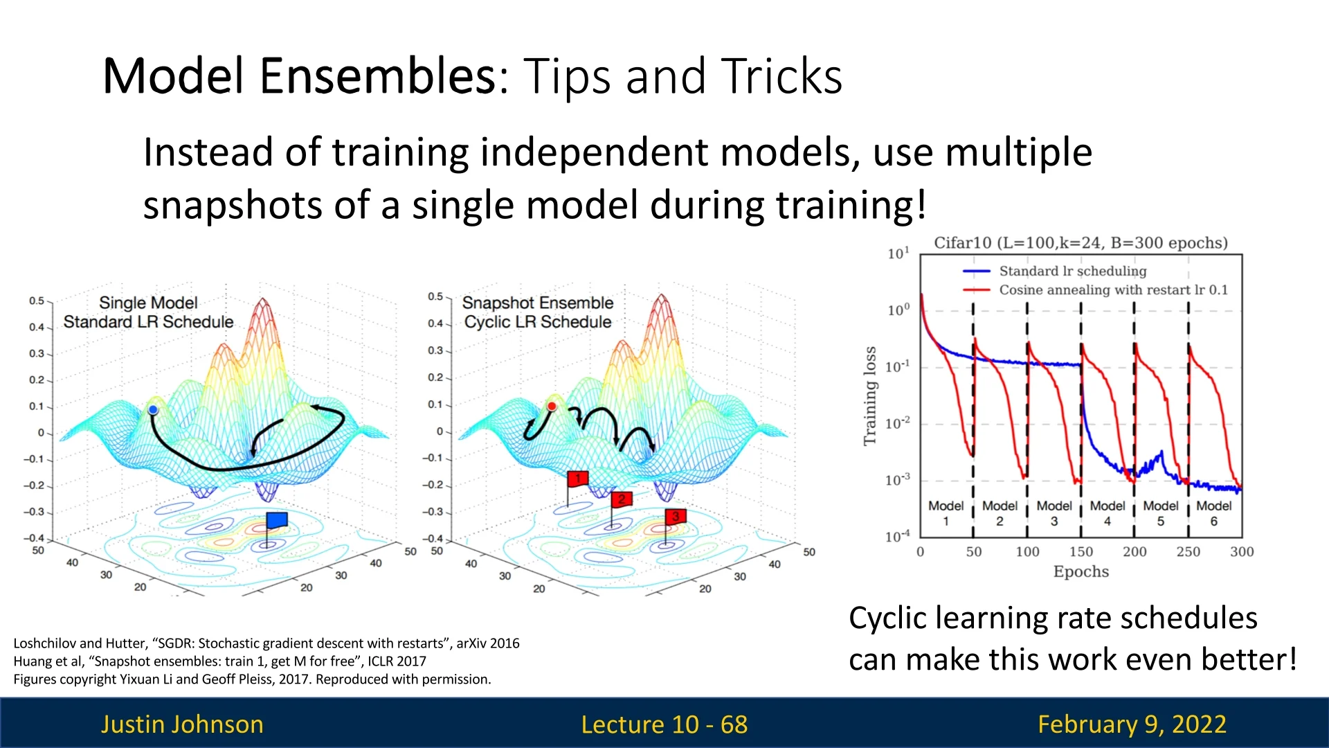
While ensembling multiple independently trained models is the most common approach, an interesting variation involves leveraging a cyclic learning rate schedule to generate multiple checkpoints from a single training run. This approach, while not mainstream, has been observed to yield performance gains without requiring us to train different unrelated models. Instead of training multiple models separately, we save several checkpoints from different training epochs (using cyclic learning rate scheduling) and ensemble their predictions at test time.
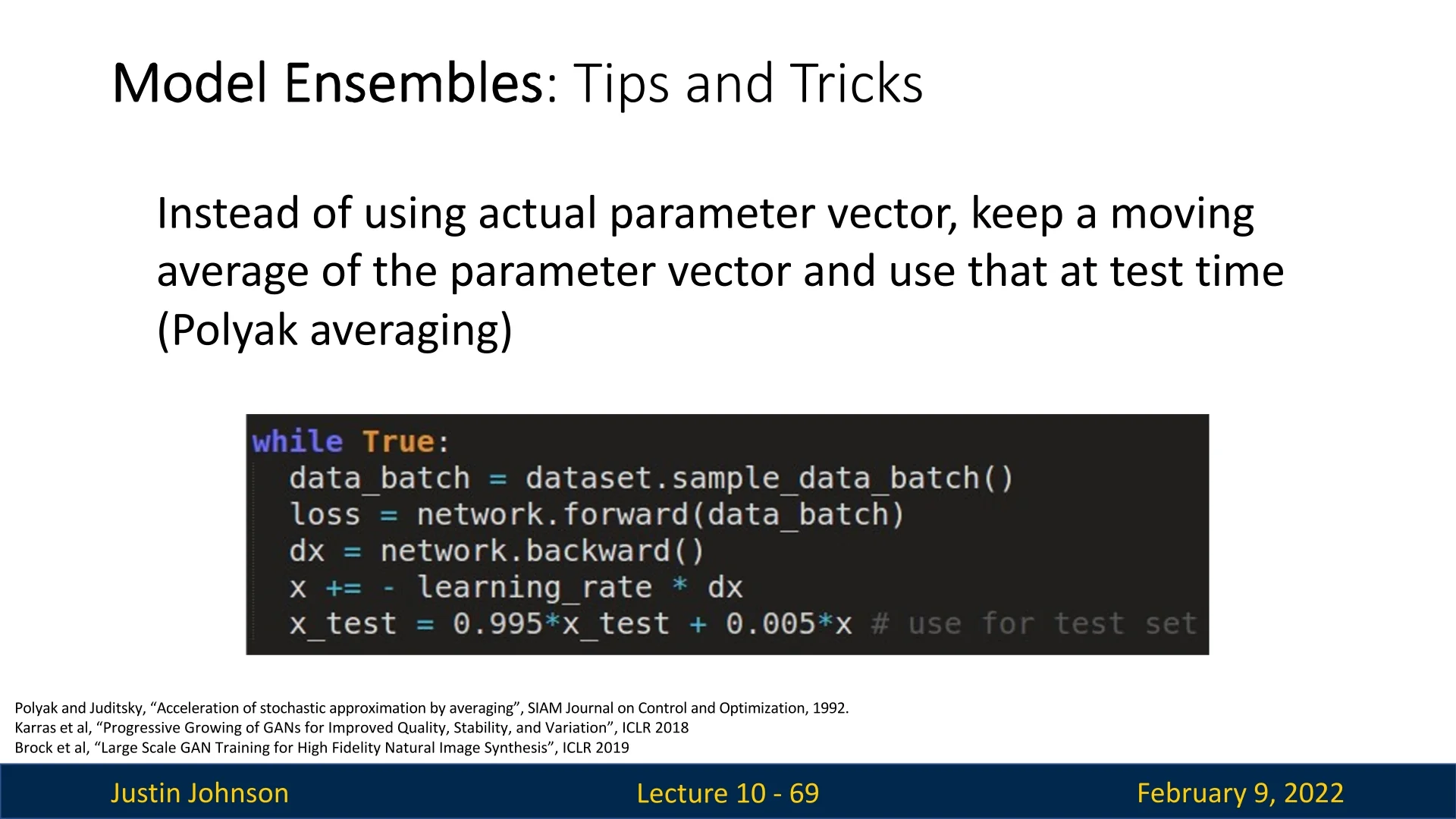
10.2.6 Exponential Moving Average (EMA) and Polyak Averaging
In large-scale generative models and other deep learning applications, researchers sometimes use Polyak averaging [498], which maintains a moving average of the model parameters over training iterations. Instead of using the final model weights from the last iteration, the model employs an exponential moving average (EMA) of the weights for evaluation: \begin {equation} \theta _{EMA} = \alpha \theta _{EMA} + (1 - \alpha ) \theta _t \end {equation} where \(\theta _t\) are the model parameters at iteration \(t\), and \(\alpha \) is a smoothing coefficient close to 1 (e.g., 0.999).
Using EMA helps smooth out loss fluctuations and reduces variance in predictions, improving robustness to noise. This technique is conceptually similar to Batch Normalization [265], but instead of maintaining moving averages of activation statistics, EMA applies to model weights.
10.3 Transfer Learning
There is a common myth that training a deep convolutional neural network (CNN) requires an extremely large dataset to achieve good performance. However, this is not necessarily true if we leverage transfer learning. Transfer learning has become a fundamental part of modern computer vision research, allowing models trained on large datasets like ImageNet to generalize well to new tasks with significantly smaller datasets.
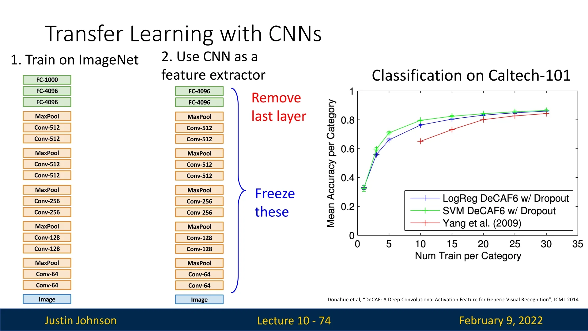
The key idea behind transfer learning is straightforward:
- 1.
- Train a CNN on a large dataset such as ImageNet.
- 2.
- Remove the last layer(s), which are specific to the original dataset.
- 3.
- Freeze the remaining layers and use them as a feature extractor.
- 4.
- Train a new classifier (e.g., logistic regression, SVM, or a shallow neural network) on top of the extracted features.
This concept is applicable not only to CNNs but also to other architectures like Transformers, making it highly versatile across various deep learning domains. It enables impressive performance even on datasets with limited training samples.
One compelling example of the impact of transfer learning can be observed in the classification performance on the Caltech-101 dataset. The previous state-of-the-art methods (before deep learning, shown in red) performed significantly worse compared to deep learning-based approaches. By using AlexNet, pretrained on ImageNet, and applying a simple classifier such as logistic regression (blue) or an SVM (green) on top of the learned feature representations, performance improved dramatically—even with limited training data.
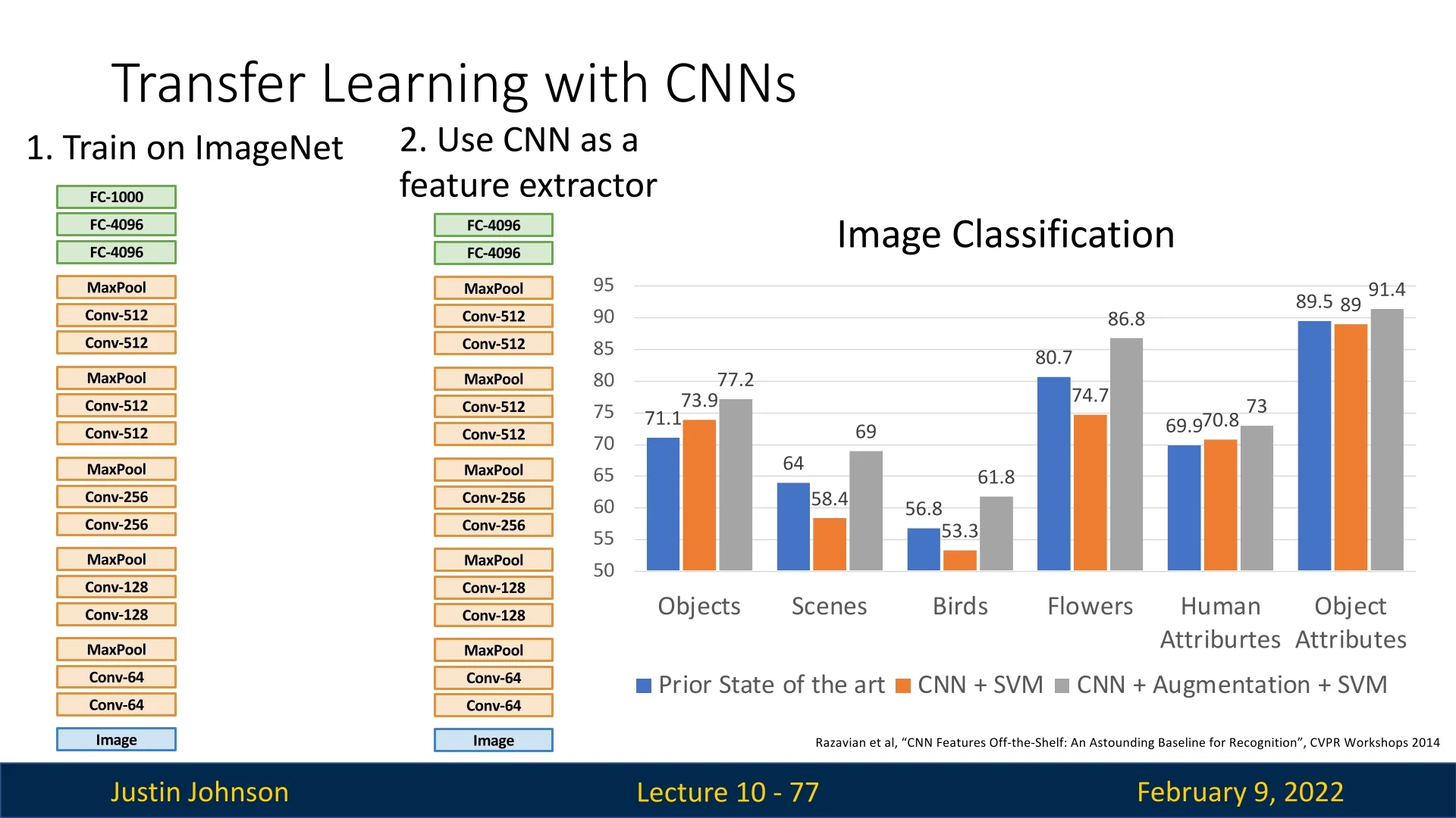
The transfer learning approach is effective across a wide range of image classification tasks. This simple fine-tuning strategy significantly outperforms tailored solutions designed for specific datasets, as demonstrated across multiple datasets, including object recognition, scene classification, fine-grained tasks such as bird and flower classification, and human attribute recognition 10.23.
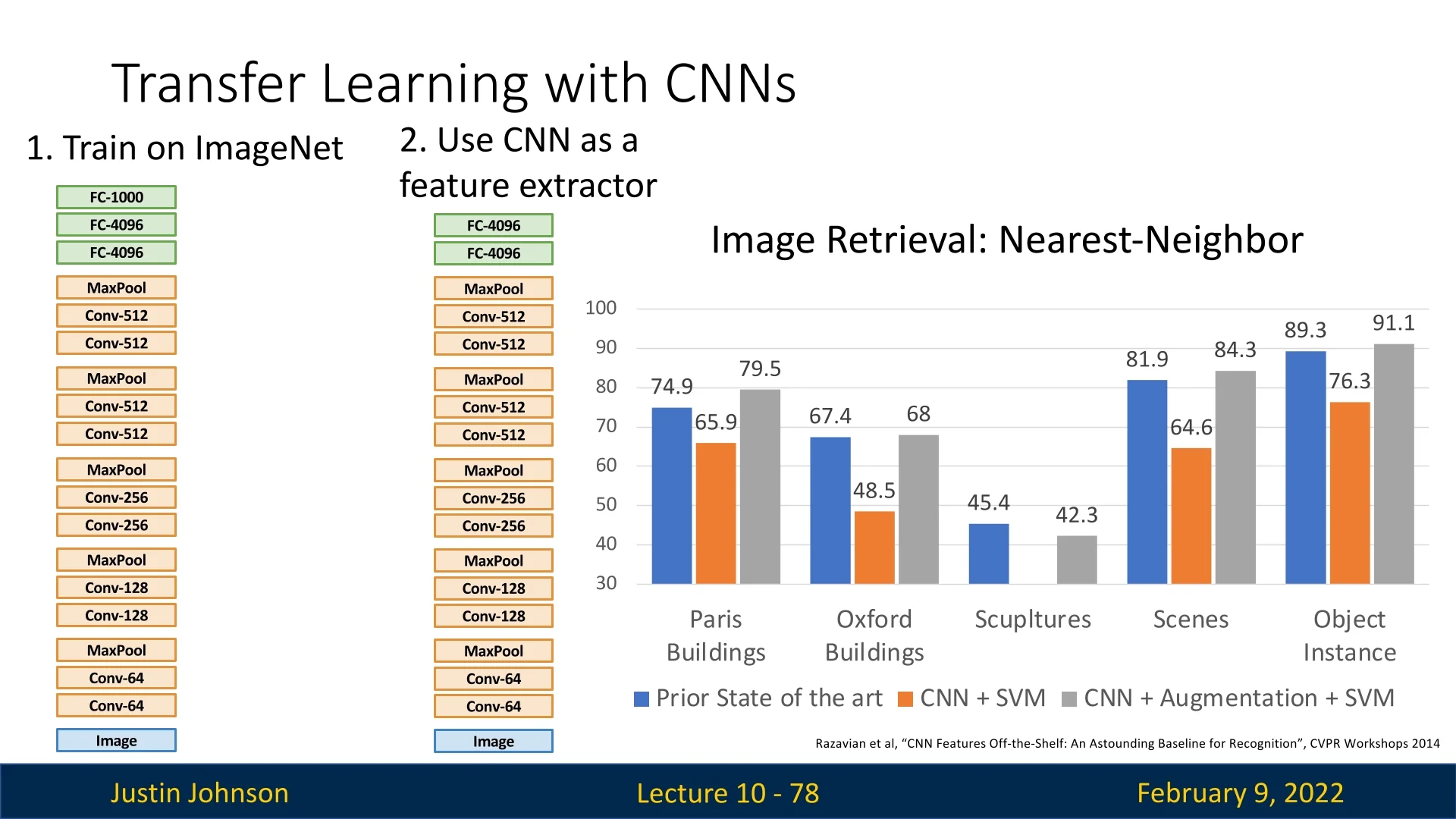
Transfer learning has also demonstrated its effectiveness in image retrieval tasks. By applying simple nearest-neighbor search on top of the extracted CNN features, deep learning-based methods outperformed previous solutions in tasks such as Paris Buildings, Oxford Buildings, etc.
For larger datasets, a more advanced transfer learning approach, known as fine-tuning, can yield even better results.
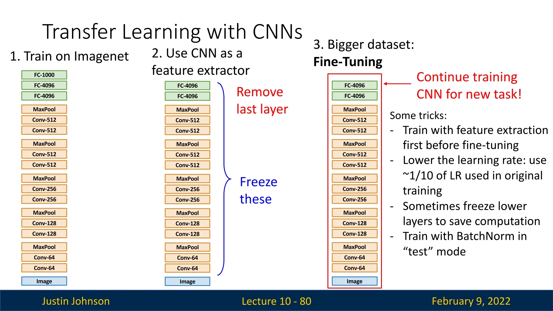
Rather than freezing all layers except the last, we can allow some of the later layers to continue training while keeping the earlier layers fixed. The reasoning behind this approach is:
- Early layers learn general low-level features (edges, textures) that remain useful across datasets.
- Later layers capture more fine-grained details that can be adapted to the new task.
To fine-tune effectively, we typically:
- Train a classifier on top of the CNN while keeping the lower layers frozen.
- Once the classifier is trained, gradually unfreeze higher layers and train with a lower learning rate (typically ˜\(1/10\) of the original learning rate).
- Optionally, freeze early layers entirely while fine-tuning only the last few layers.
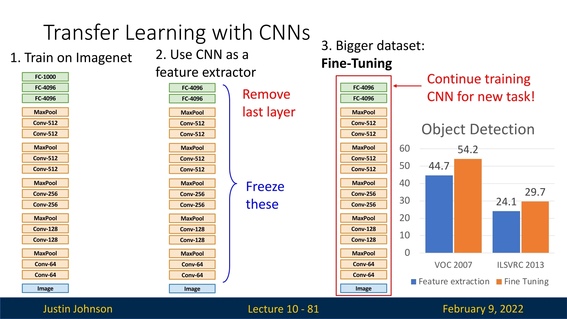
Fine-tuning has been shown to provide a substantial performance boost over feature extraction alone. For example, object detection on the VOC 2007 dataset improved from 44.7% to 54.2%, while performance on ILSVRC 2013 increased from 24.1% to 29.7% when fine-tuning was applied.
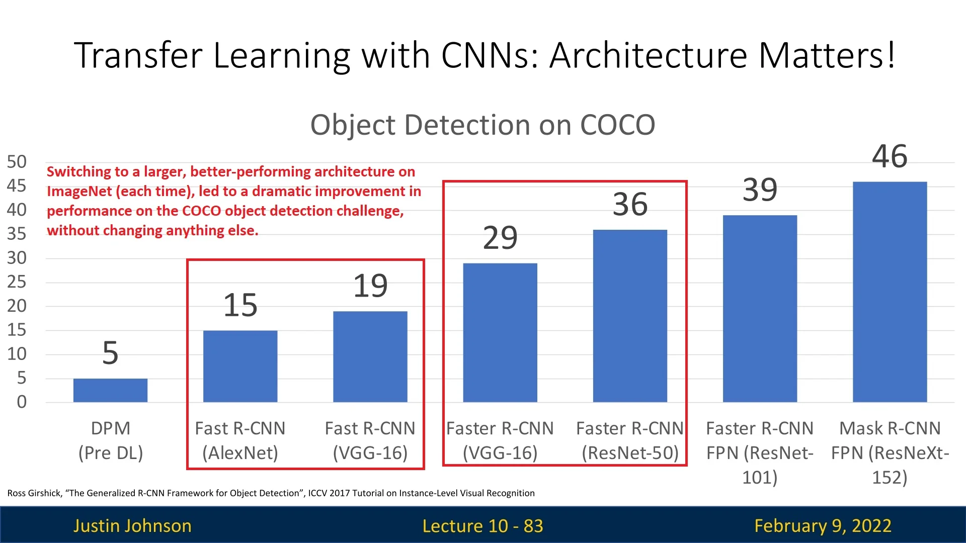
Typically, models chosen for transfer learning are those that perform well on ImageNet. Over the years, simply switching to better pretrained models on ImageNet has significantly improved downstream tasks, such as object detection on COCO.
Transfer learning remains one of the most powerful techniques in deep learning, enabling high-performance models even in data-scarce scenarios and reducing the need for expensive training from scratch. By utilizing pretrained models and fine-tuning them effectively, researchers and practitioners can achieve state-of-the-art results across a wide variety of vision tasks.
10.3.1 How to Perform Transfer Learning with CNNs?
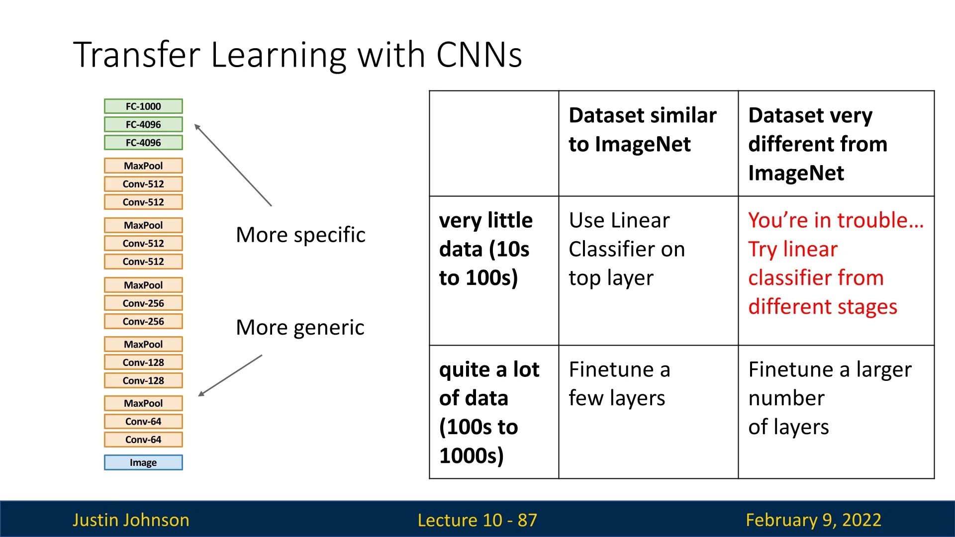
While transfer learning is a powerful technique, the question remains: how should we apply it effectively when working with CNNs? The optimal transfer learning strategy depends on two main factors:
- Similarity to ImageNet: How closely the new dataset resembles ImageNet in terms of image distribution and task.
- Dataset Size: Whether the dataset is large or small.
A practical guideline for choosing a transfer learning strategy is summarized in the following 2x2 table:
- 1.
- Small dataset, similar to ImageNet: Use a linear classifier on top of the frozen CNN features.
- 2.
- Large dataset, similar to ImageNet: Fine-tune only a few of the later layers while keeping early layers frozen.
- 3.
- Large dataset, different from ImageNet: Fine-tune a larger portion of the CNN, allowing it to adapt to the new domain.
- 4.
- Small dataset, different from ImageNet: This is the most challenging scenario. One can attempt either a linear classifier or fine-tuning, but success is not guaranteed.
10.3.2 Transfer Learning Beyond Classification
Transfer learning is pervasive—it has become the norm rather than the exception. Beyond standard image classification, it is widely used in tasks such as object detection and image captioning. Researchers even experiment with pretraining different parts of a model on separate datasets before integrating them into a unified model, fine-tuning it for specific tasks.
One such example is presented in [821], where transfer learning is applied in a multi-stage manner:
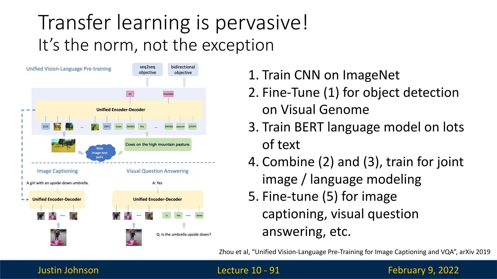
- 1.
- Train a CNN on ImageNet for feature extraction.
- 2.
- Fine-tune the CNN on Visual Genome for object detection.
- 3.
- Train a BERT-based language model on large-scale text corpora.
- 4.
- Combine the fine-tuned CNN and BERT model for joint image-language modeling.
- 5.
- Fine-tune the resulting model for tasks such as image captioning and visual question answering (VQA).
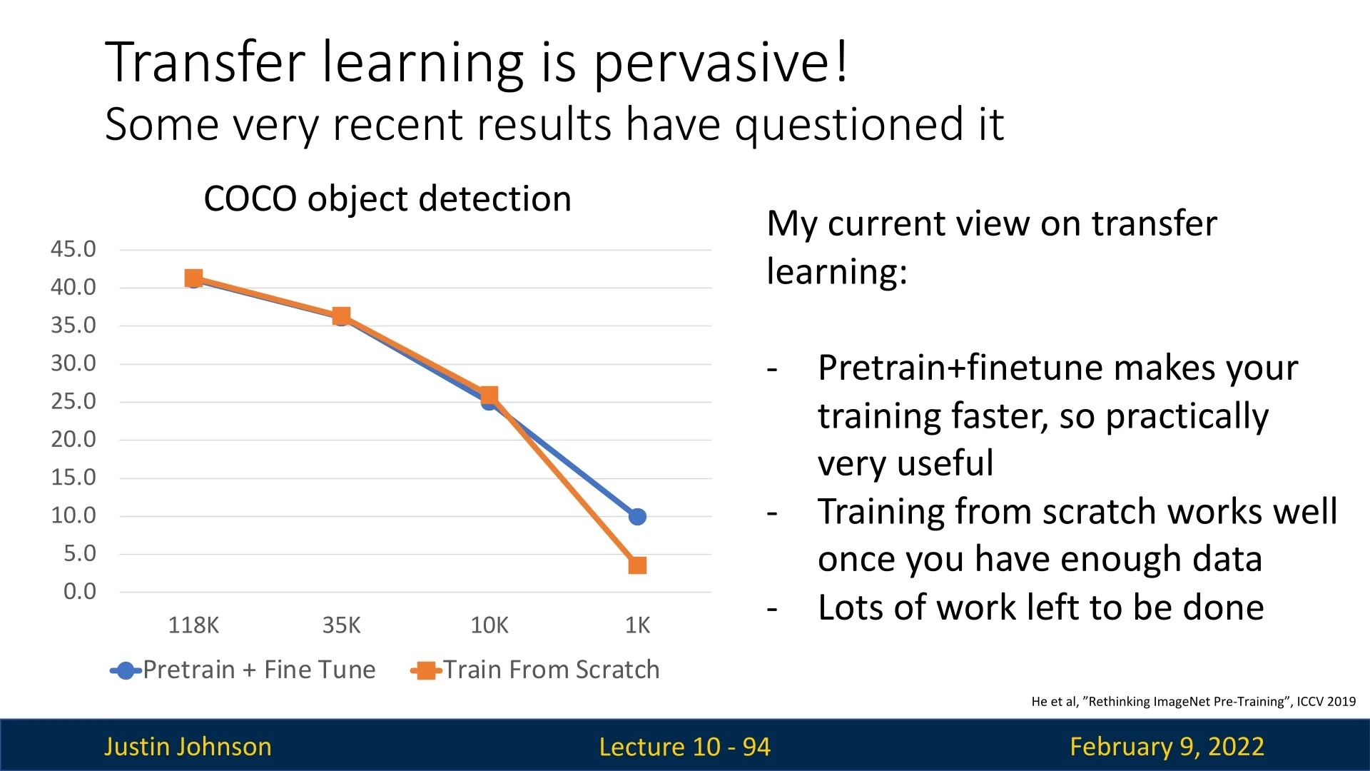
10.3.3 Does Transfer Learning Always Win?
While transfer learning is highly effective, recent research suggests that training from scratch can sometimes be competitive. In [214], researchers examined whether ImageNet pretraining is necessary for object detection and found that training from scratch can work well but requires approximately three times the training time to match performance achieved by pretraining.
Despite this, pretraining followed by fine-tuning remains superior when datasets are small (e.g., only tens of samples per class). This result is intuitive—having access to pretrained features provides a strong starting point in cases where the available data is insufficient to learn meaningful representations from scratch. Moreover, the efficiency of transfer learning makes it practically useful even for large-scale datasets. Hence, it is always recommended to try transfer learning when we aim to solve CV tasks.
Ultimately, while collecting more data remains the best way to improve model performance, transfer learning provides a practical, efficient, and effective solution for adapting pretrained models to new tasks.
Enrichment 10.3.4: Regularization in the Era of Finetuning
1. Freezing Most of the Backbone In most fine-tuning pipelines, the majority of the model—especially early and mid-level layers of a pretrained network—is kept frozen to retain its general-purpose features. Only a subset of late-stage layers or newly added modules (e.g., classification heads) are updated:
- Why freeze? To preserve learned representations from large-scale datasets (e.g., ImageNet, CLIP) and prevent catastrophic forgetting when adapting to smaller datasets [241].
- Minimal regularization need: Since frozen parameters are not updated, there’s no need to regularize them. Even in partially frozen setups (e.g., layer-wise learning rate decay), mild \(\ell _2\) or batch norm tuning may help—but only when the domain shift is significant.
2. Regularizing Small Trainable Heads: Caution With Dropout When fine-tuning adds only a shallow classification head (e.g., a 1–2 layer MLP or linear probe), strong regularization like dropout may be too aggressive:
- For shallow heads (1–2 layers): Dropout is rarely used unless the dataset is very small or prone to label noise. Lighter \(\ell _2\) weight decay is typically preferred.
- For deeper heads (3+ layers): Moderate dropout (e.g., 0.3–0.5) becomes more effective, especially in low-data settings where overfitting risk increases.
3. Training From Scratch on Large Datasets When training a network from scratch (e.g., ViTs or CNNs) on high-volume datasets like ImageNet-21k or JFT:
- Large batches make BN optional: If batch size is large, the per-batch statistics become stable, and some models even omit BN entirely [790, 134].
- Data abundance reduces overfitting risk: Regularization is still used, but it shifts from aggressive \(\ell _2\) penalties toward more gentle implicit regularizers such as data augmentations.
4. Implicit and Soft Regularization Prevail In both fine-tuning and large-scale training, modern pipelines increasingly lean on:
- Data augmentation: mixup, CutMix [770], RandAugment [114] are now dominant forms of regularization.
- Light weight decay or dropout: Rather than large-scale penalties, milder explicit regularizers are combined with augmentation and pretraining.
5. Summary In modern transfer learning workflows:
- Most regularization effort is applied to small newly-trained modules (e.g., MLPs).
- Dropout is more effective when deeper heads are trained (3+ layers), but is sometimes too harsh for smaller heads.
- BN and \(\ell _2\) decay are unnecessary for frozen layers, and are often minimal even in unfrozen ones, if used at all.
- Augmentations and large pretraining data serve as primary generalization & regularization tools in the fine-tuning and large datasets era.
1For SGD this is classical momentum; for AdamW interpret \(m_t\) as the time-varying \(\beta _1(t)\).