Lecture 3: Linear Classifiers
3.1 Linear Classifiers: A Foundation for Neural Networks
Linear classifiers are a cornerstone of machine learning and form one of the most fundamental building blocks for modern neural networks.

As illustrated in Figure 3.1, neural networks are constructed by stacking basic components, with linear classifiers serving as one of the foundational elements. Despite their simplicity, linear classifiers play a critical role in providing a structured, parametric framework that maps raw input data to class scores. They naturally extend to more sophisticated architectures, such as neural networks and convolutional neural networks (CNNs).
This chapter focuses on linear classifiers and their role in classification problems. To develop a comprehensive understanding of their behavior and limitations, we will examine linear classifiers from three perspectives:
- Algebraic Viewpoint: Frames the classifier as a mathematical function, emphasizing the score computation as a weighted combination of input features and biases.
- Visual Viewpoint: Reveals how the classifier learns templates for each class and compares them with input images, highlighting its behavior as a form of template matching.
- Geometric Viewpoint: Interprets the classifier’s decision-making process in high-dimensional spaces, with hyperplanes dividing the space into regions corresponding to different classes.
These viewpoints not only help us understand the mechanics of linear classifiers but also shed light on their inherent limitations, such as their inability to handle non-linearly separable data or account for multiple modes in class distributions.
Finally, we introduce the key components of linear classifiers:
- A score function that maps input data to class scores.
- A loss function that quantifies the model’s performance by comparing predictions to ground truth labels.
While this chapter will focus on understanding these perspectives and defining loss functions, we will leave the topics of optimization and regularization for the next lecture, where we will discuss how to effectively train and refine linear classifiers.
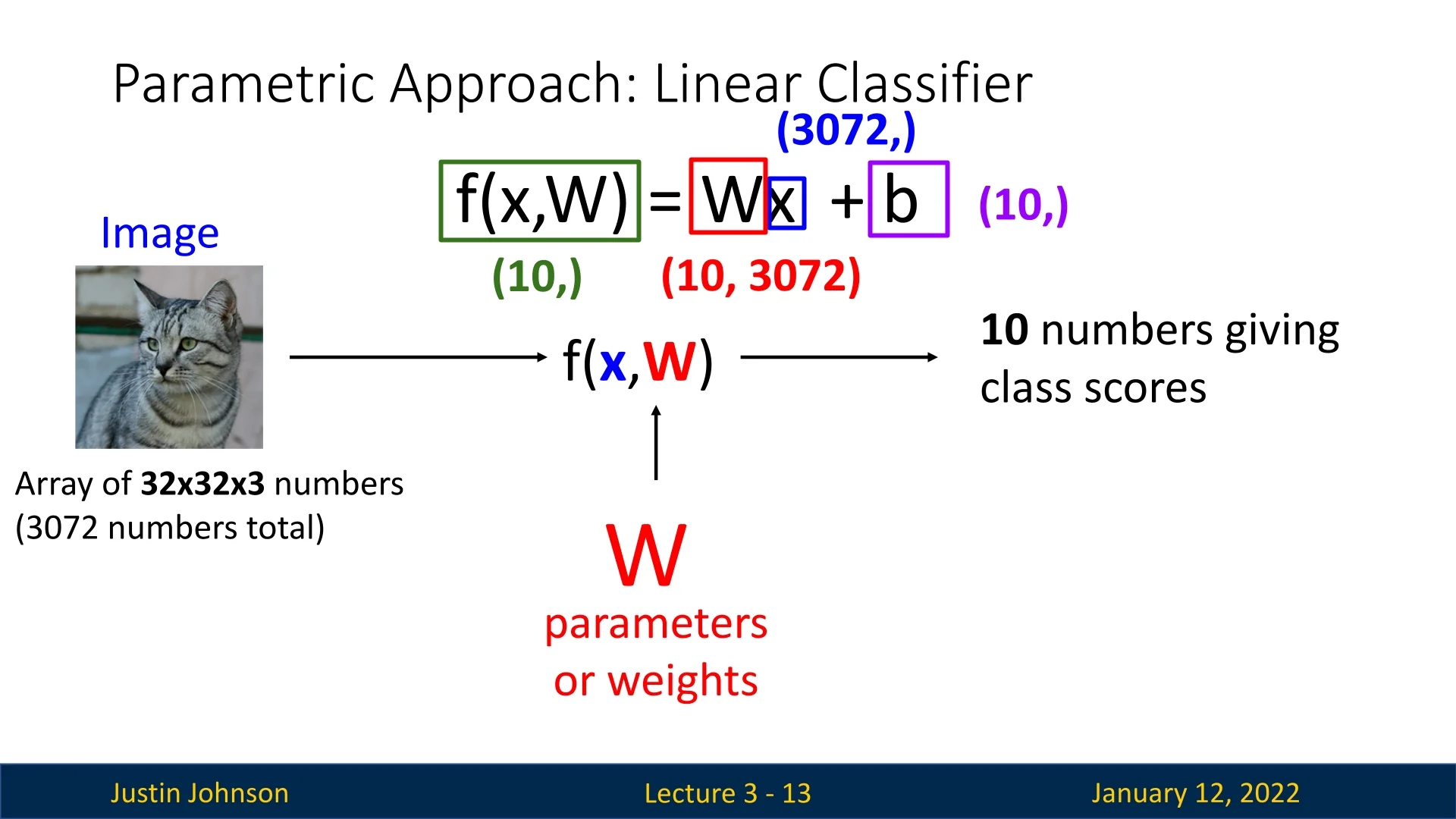
As seen in Slide 3.2, linear classifiers adopt a parametric approach where the input image \(\mathbf {x}\) (e.g., a \(32 \times 32 \times 3\) RGB image of a cat) is flattened into a single vector of pixel values of length \(D = 3072\). This flattening is performed consistently across all input images to maintain structural uniformity. Given \(K = 10\) classes, the classifier outputs 10 scores, one for each class. This is achieved using the function: \[ f(\mathbf {x}, W, \mathbf {b}) = W\mathbf {x} + \mathbf {b}, \] where \(W\) is a learnable weight matrix of shape \(K \times D\), and \(\mathbf {b}\) is a learnable bias vector of shape \(K\).
The weight matrix \(W\) and the bias term \(\mathbf {b}\) work together to define the decision boundary in a linear classifier. To build intuition, consider the simple example of a linear equation \(y = mx + b\) in two dimensions. In this equation:
- \(m\) determines the slope of the line, dictating how steeply it tilts.
- \(b\) shifts the line vertically, allowing it to move up or down along the \(y\)-axis. This effectively changes where the line crosses the axis, without altering its slope.
Similarly, in a linear classifier, the decision boundary is represented as \(W \mathbf {x} + \mathbf {b} = 0\), where:
- The weight matrix \(W\) determines the orientation and steepness of the decision boundary in the input space by defining how the features \(\mathbf {x}\) combine to produce class scores.
- The bias term \(\mathbf {b}\), independent of the input features \(\mathbf {x}\), offsets the decision boundary. This shifts the hyperplane in the feature space, much like \(b\) in \(y = mx + b\) shifts the line vertically.
Enrichment 3.1.1: Understanding the Role of Bias in Linear Classifiers
The bias term \(\mathbf {b}\) in linear classifiers allows the decision boundary to shift, enabling the model to handle data distributions that are not centered at the origin. This flexibility is essential, as demonstrated in the following example:
Example 3.1 Consider a classification task in 2D space with two data points:
- Red point (Class 1): \((1, 1)\).
- Blue point (Class 2): \((2, 2)\).
The decision boundary is defined as: \[ W \mathbf {x} + b = 0 \implies -x - y + b = 0. \]
Without Bias (\(b=0\)): The decision boundary simplifies to: \[ w_1 x + w_2 y = 0 \quad \Longrightarrow \quad y = -\tfrac {w_1}{w_2}\,x. \] Suppose we want the model to classify: \[ \mbox{Red point }(1,1)\;\mbox{on one side, and Blue point }(2,2)\;\mbox{on the other.} \] Concretely, for \((x,y)\) in Class 1, we want: \[ w_1\cdot 1 + w_2\cdot 1 > 0, \] and for Class 2 we want: \[ w_1\cdot 2 + w_2\cdot 2 < 0. \] These inequalities become: \[ \begin {cases} w_1 + w_2 > 0, \\ 2w_1 + 2w_2 < 0. \end {cases} \] Dividing the second by 2 yields: \[ w_1 + w_2 < 0, \] which directly contradicts \(w_1 + w_2 > 0\). Hence, no choice of \((w_1, w_2)\) can separate the points without a bias.
- The decision boundary becomes \(y = -x + 3\), shifting the line upward.
- The red point \((1, 1)\) satisfies \(-x - y + 3 > 0\) (classified as red).
- The blue point \((2, 2)\) satisfies \(-x - y + 3 < 0\) (classified as blue).
- The bias term enables correct separation of the two points.
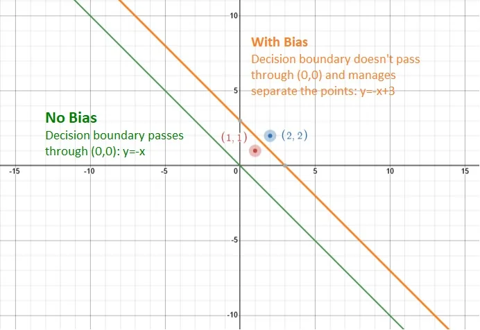
Key Insight: Without the bias term, the decision boundary is constrained to pass through the origin, making it impossible to correctly separate the two points. Adding a bias term shifts the boundary, enabling proper classification.
This concept generalizes beyond toy 2D problems. In higher-dimensional spaces, the bias term provides the flexibility to shift hyperplanes, enabling the classifier to handle real-world data distributions that are not centered at the origin. Without this flexibility, the model would struggle to adapt to datasets where the mean of the input features is non-zero or misaligned with the origin.
3.1.1 A Toy Example: Grayscale Cat Image
To build a strong foundation for understanding how linear classifiers work, let us consider a toy example of a grayscale \(2 \times 2\) image of a cat. Each pixel has a value ranging from 0 to 255, representing its grayscale intensity. Although real cat images are much larger, this simplified scenario helps illustrate the key principles with ease.
- Image Representation: The \(2 \times 2\) image is flattened into a column vector with 4 entries, denoted as: \[ \mathbf {x} = [x_1, x_2, x_3, x_4]^T. \]
- Weight Matrix \(\mathbf {W}\): The weight matrix \(\mathbf {W}\) has \(K\) rows (one for each class) and 4 columns (one for each pixel). Each row of \(\mathbf {W}\) corresponds to a specific class and determines the influence of each pixel on the classification score.
- Matrix Multiplication: The input vector \(\mathbf {x}\) is multiplied with the weight matrix \(\mathbf {W}\) to produce a vector of scores: \[ \mathbf {s} = \mathbf {W} \mathbf {x}, \] where \(\mathbf {s} = [s_1, s_2, \dots , s_K]^T\) represents the scores for \(K\) classes.
- Bias Term: A bias vector \(\mathbf {b}\) of size \(K\) is added to the score vector:\(\mathbf {o} = \mathbf {s} + \mathbf {b},\) resulting in the final output vector \(\mathbf {o}\), where each element represents the adjusted score for a class.
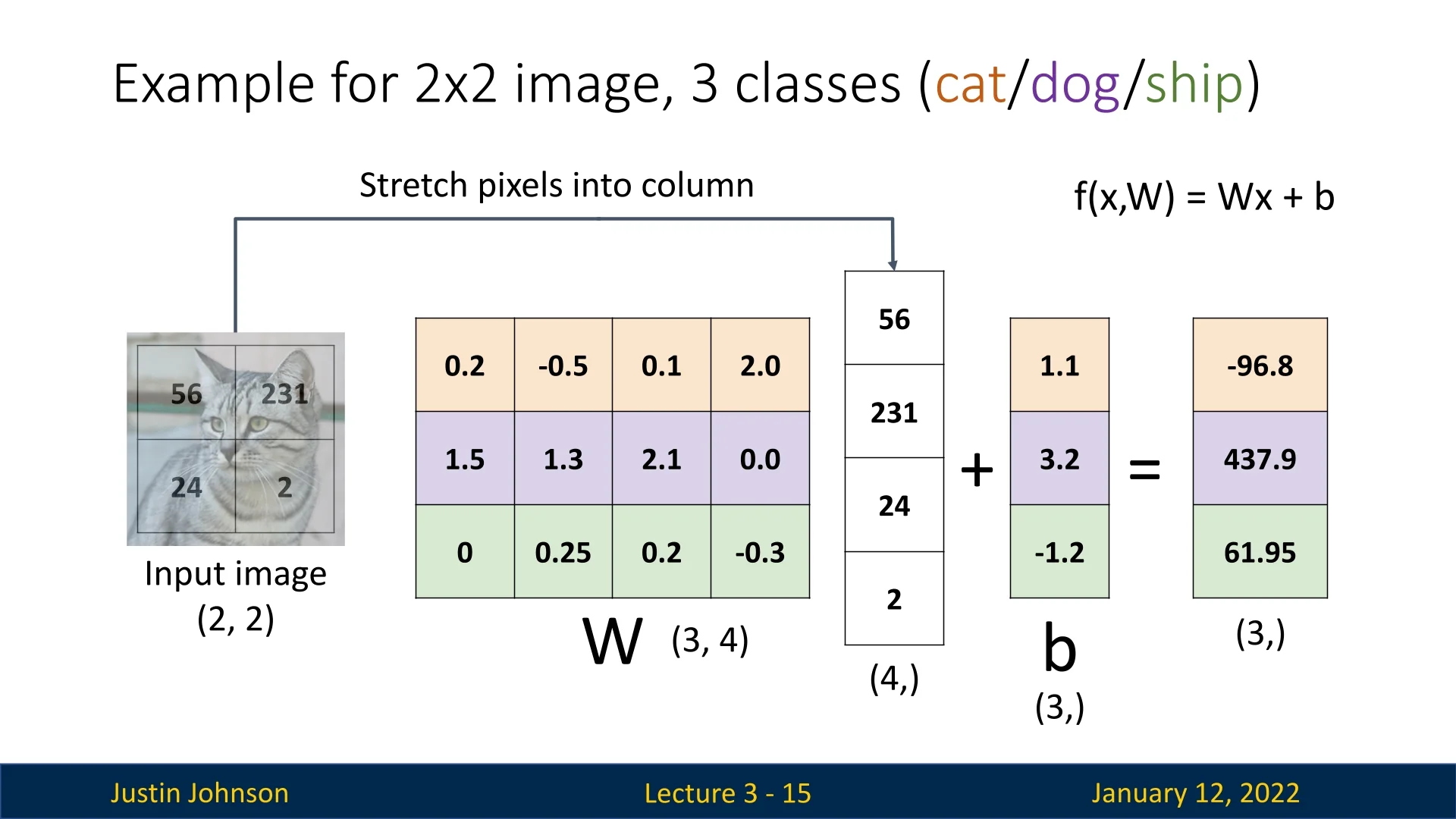
This simple yet powerful operation demonstrates how linear classifiers map raw data (pixel values) to class scores using a combination of learned weights and bias terms.
3.1.2 The Bias Trick
In linear classifiers, the bias term \(\mathbf {b}\) plays a critical role in adjusting the decision boundary. An alternative way to incorporate the bias is through a technique called the bias trick, which eliminates the explicit bias vector by augmenting the input data and weight matrix. This approach is commonly used when the input data naturally has a vector form, such as in tabular datasets.
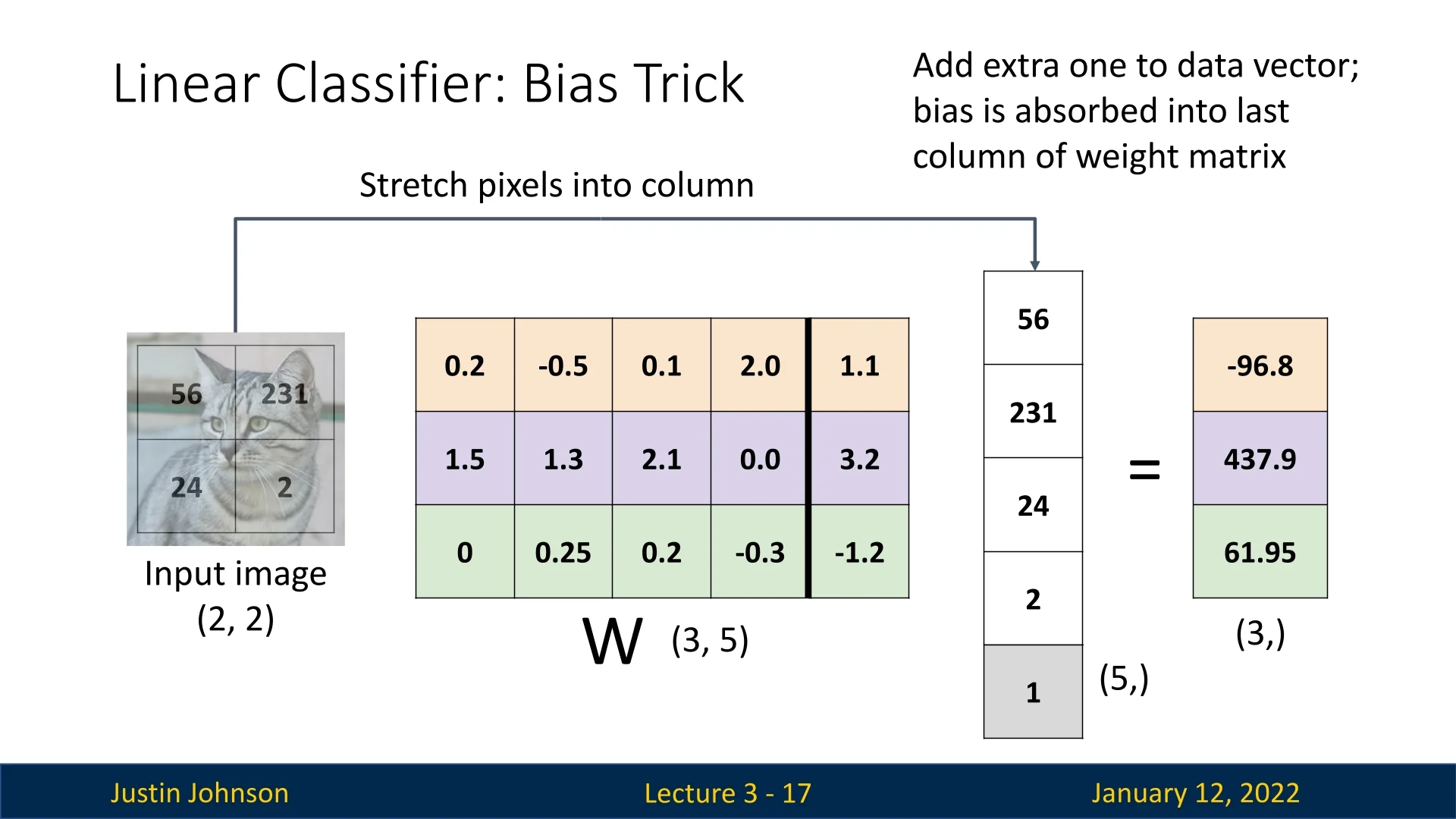
How the Trick Works:
- Augmented Input Representation: To absorb the bias term into the weight matrix, we append an additional constant value of \(1\) to the input feature vector. If the original feature vector is \(\mathbf {x} = [x_1, x_2, \dots , x_D]^T\), the augmented representation becomes: \[ \mathbf {x}' = [x_1, x_2, \dots , x_D, 1]^T. \]
- Augmented Weight Matrix: The weight matrix \(\mathbf {W}\) is updated by adding a new column corresponding to the bias. If \(\mathbf {W}\) initially has dimensions \(K \times D\), the augmented matrix becomes \(K \times (D+1)\), where the last column holds the bias values for each class.
- Unified Matrix Multiplication: The score computation becomes: \[ \mathbf {s} = \mathbf {W} \mathbf {x}', \] effectively absorbing the bias into the augmented weight matrix.
Example with Cat Image (Slide 3.5)
To demonstrate the bias trick in action, consider the toy example of a \(2 \times 2\) grayscale image of a cat introduced earlier (Slide 3.4). Initially, the image was flattened into a vector of 4 pixels, \([p_1, p_2, p_3, p_4]^T\). Using the bias trick, we augment this vector by appending a constant value of \(1\), resulting in: \[ \mathbf {x}' = [p_1, p_2, p_3, p_4, 1]^T. \]
Simultaneously, the weight matrix \(\mathbf {W}\), originally of shape \(K \times 4\), is augmented to \(K \times 5\) by adding a new column to account for the bias term. The computation of class scores becomes: \[ \mathbf {s} = \mathbf {W} \mathbf {x}', \] where the augmented weight matrix seamlessly integrates the effect of the bias.
Advantages of the Bias Trick:
- Simplified Notation: The trick reduces the need for separate terms in the computation, allowing the bias and weights to be handled in a unified framework.
- Ease of Implementation: In frameworks where data is inherently vectorized (e.g., certain numerical libraries), this method simplifies coding and matrix operations.
- Theoretical Insights: This technique emphasizes that the bias term is simply an additional degree of freedom, equivalent to a constant input feature with fixed weight.
Limitations in Computer Vision: In computer vision, the bias trick is less frequently used. For example, in convolutional neural networks (CNNs), this approach does not translate well because the input is often represented as multi-dimensional tensors (e.g., images), and the convolution operation does not naturally accommodate the bias trick. Additionally:
- Separate Initialization: Bias and weights are often initialized differently in practice. For instance, weights may be initialized randomly, while biases might start at zero to avoid influencing initial predictions.
- Flexibility in Training: Treating bias and weights separately allows more nuanced adjustments during regularization or optimization.
When to Use the Bias Trick: The bias trick is particularly useful for datasets where the input data is naturally represented as a vector (e.g., tabular data or flattened image data). It simplifies the mathematical formulation and is computationally efficient in these scenarios. However, when working with more complex data structures, such as images in their raw tensor form, separating the bias term often provides more flexibility and practical utility.
This technique highlights the elegance and adaptability of linear classifiers, demonstrating how small changes in representation can simplify computations while maintaining mathematical equivalence.
3.2 Linear Classifiers: The Algebraic Viewpoint
The algebraic viewpoint provides an elegant mathematical framework to understand linear classifiers. It emphasizes the role of the weight matrix \(\mathbf {W}\) and the bias vector \(\mathbf {b}\) in transforming input features into scores for each class. This perspective also highlights certain intrinsic properties and limitations of linear classifiers.
3.2.1 Scaling Properties and Insights
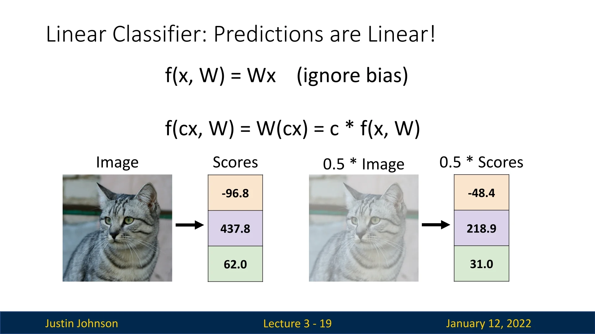
Linear classifiers exhibit a key property: their output scores scale linearly with the input. Consider a scaled input \(\mathbf {x}' = c\mathbf {x}\) (where \(c > 0\) is a constant). When passed through a classifier without a bias term, the output becomes: \[ f(\mathbf {x}', \mathbf {W}) = \mathbf {W}(c\mathbf {x}) = c \cdot f(\mathbf {x}, \mathbf {W}). \]
This means that scaling the input by a constant \(c\) directly scales the output scores by \(c\). Slide 3.6 illustrates this with a practical example. A grayscale image of a cat, when uniformly brightened or darkened (scaling all pixel values by \(c\)), results in scaled class scores. Humans can still easily recognize the cat, but the classifier’s output scores are proportionally reduced. For instance: \[ f(\mathbf {x}, \mathbf {W}) = [2.0, -1.0, 0.5], \quad f(c\mathbf {x}, \mathbf {W}) = [1.0, -0.5, 0.25] \quad \mbox{(for \(c = 0.5\))}. \]
This feature of linear classifiers may or may not be desirable, depending on the choice of loss function:
- If the loss function focuses on relative scores, such as cross-entropy, the scaling has no effect because the final predictions depend only on the relative differences between scores.
- However, in other contexts, absolute score magnitudes might be important, and scaling could introduce issues.
3.2.2 From Algebra to Visual Interpretability
While the algebraic viewpoint is powerful for mathematical formulation, it can sometimes obscure the intuition behind the classifier’s behavior. A useful trick to bridge this gap involves reshaping the rows of the weight matrix \(\mathbf {W}\) into image-like blocks.
Each row of \(\mathbf {W}\) corresponds to one class, and reshaping it into the dimensions of the input image allows us to visualize what the classifier ”sees” for each class. These visualizations can provide insight into:
- What features the classifier considers important for each class.
- How the classifier might misinterpret or confuse one class with another.
- Biases or artifacts present in the dataset, as reflected in the learned weights.
This interpretation naturally leads into the Visual Viewpoint, which we will explore in detail in subsequent sections. By combining algebraic rigor with visual insights, we can better understand the strengths and limitations of linear classifiers.
3.3 Linear Classifiers: The Visual Viewpoint
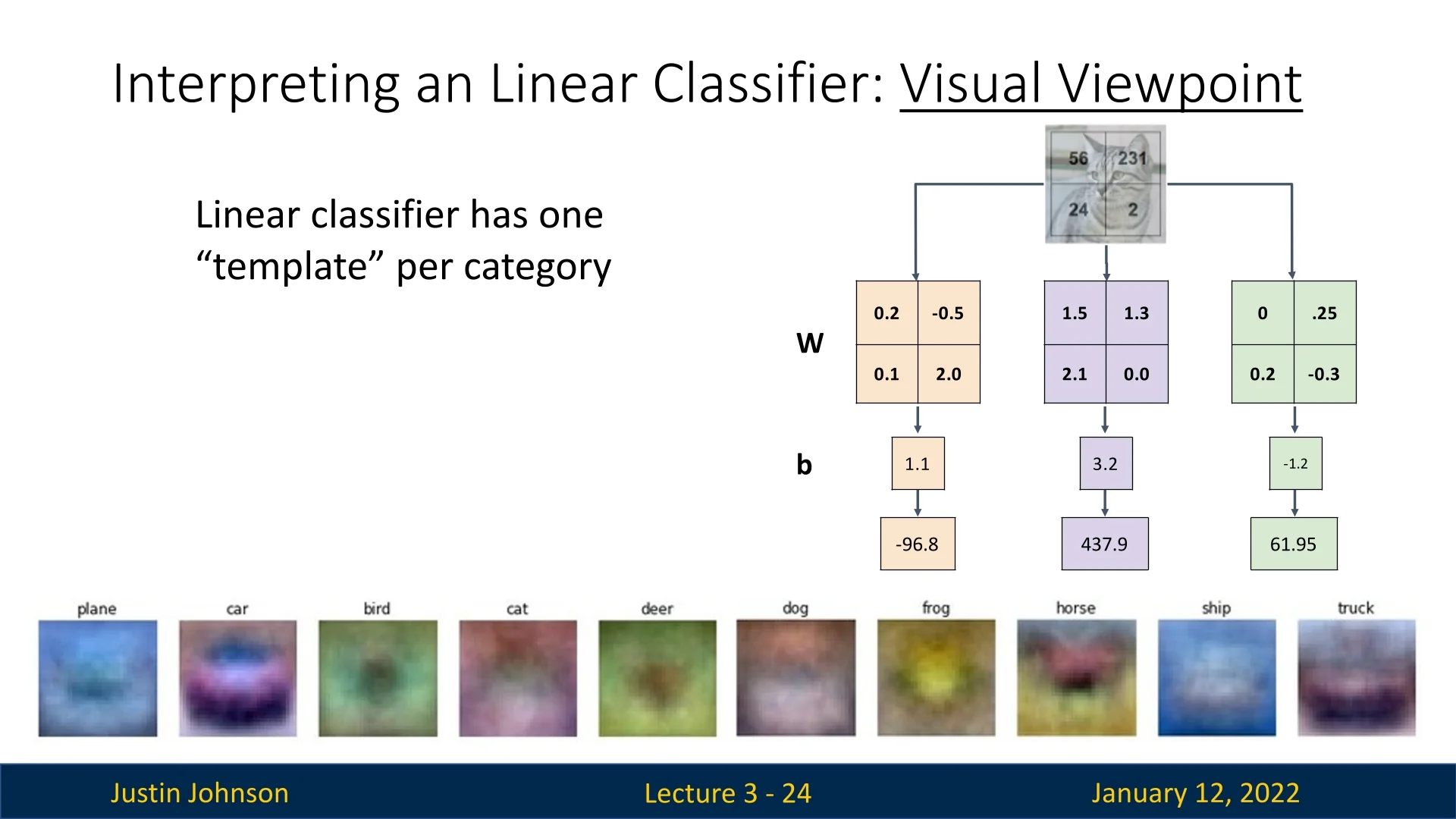
The visual viewpoint provides an intuitive way to interpret the behavior of linear classifiers by visualizing the rows of the weight matrix \(\mathbf {W}\) reshaped into the input image’s dimensions. This visualization helps us understand what the classifier ”learns” during training and highlights its strengths and limitations.
3.3.1 Template Matching Perspective
In a linear classifier, each row of the weight matrix \(\mathbf {W}\) corresponds to a specific output class. By reshaping these rows into the shape of the input image, we can view them as class-specific templates. The score for a given class is computed by taking the inner product (dot product) between the input image and the corresponding template. This process effectively performs template matching, where the templates are learned from data.
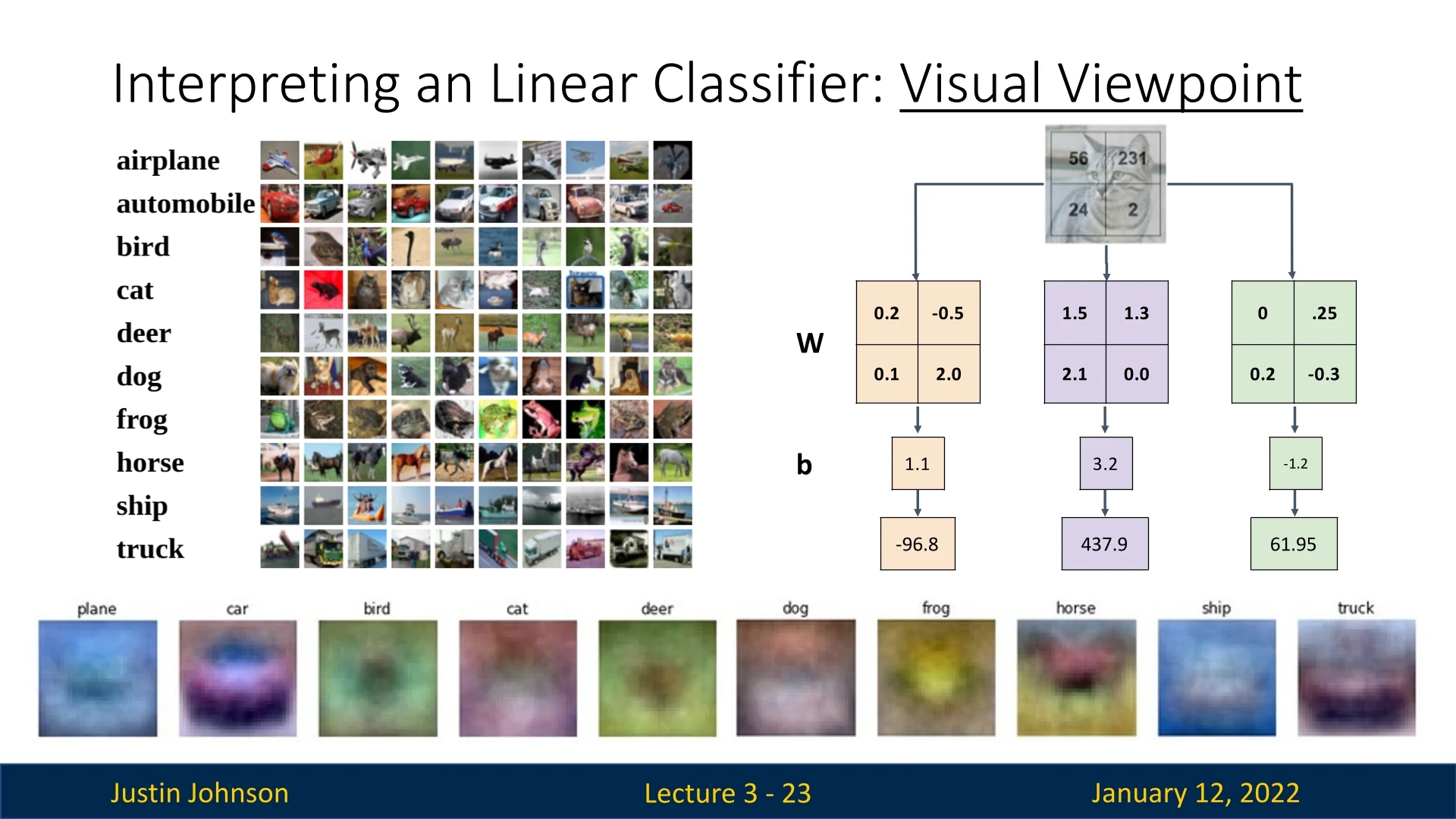
Figure 3.7 illustrates how the rows of \(\mathbf {W}\) can be visualized as templates. The inner product measures how well each template ”fits” the input image, assigning a score to each class.
This method can be compared to Nearest Neighbor classification:
- Instead of storing thousands of training images, a single learned template per class is used.
- The similarity is measured using the (negative) inner product rather than L1 or L2 distance.
3.3.2 Interpreting Templates
Visualizing the templates reveals the learned features for each class:
- Plane and Ship Classes: The templates for these classes are predominantly blue, reflecting the sky and ocean backgrounds common in the training set. A strong inner product with these templates may incorrectly classify other blue-background objects (e.g., a blue shirt) as planes or ships. Conversely, planes or ships on non-blue backgrounds might be misclassified.
- Horse Class: The horse class template appears to depict a two-headed horse, as it merges training images of horses facing left and right into a single representation.
- Car Class: The car class template is red, indicating a dataset bias toward red cars. This can lead to incorrect classifications for cars of other colors.
These observations highlight limitations of background sensitivity, a single template per class.
3.3.3 Python Code Example: Visualizing Learned Templates
Here’s an example using an SVM classifier (a type of linear classifier) to visualize learned templates:
# Visualize the learned weights for each class
w = svm.W[:-1, :]  # Strip out the bias term
w = w.reshape(32, 32, 3, 10)  # Reshape rows into image format
w_min, w_max = np.min(w), np.max(w)

classes = [’plane’, ’car’, ’bird’, ’cat’, ’deer’, ’dog’, ’frog’, ’horse’, ’ship’, ’truck’]

for i in range(10):
    plt.subplot(2, 5, i + 1)
    # Rescale weights to 0-255 range for visualization
    wimg = 255.0 * (w[:, :, :, i].squeeze() - w_min) / (w_max - w_min)
    plt.imshow(wimg.astype(’uint8’))
    plt.axis(’off’)
    plt.title(classes[i])
    plt.show()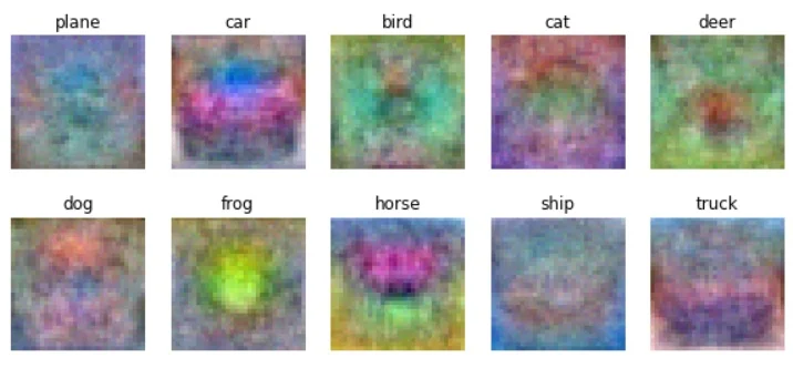
3.3.4 Template Limitations: Multiple Modes
Linear classifiers are limited by their single-template-per-class constraint:
- Categories with distinct modes (e.g., horses facing left vs. right) cannot be disentangled, as the classifier learns only one merged template.
3.3.5 Looking Ahead
While linear classifiers provide valuable insights, their limitations become apparent in real-world tasks. Neural networks, which will be introduced later, address these shortcomings by developing intermediate neurons in hidden layers. These neurons can specialize in features like ”red car” or ”blue car” and combine them into more accurate class scores, overcoming the single-template limitation of linear classifiers.
3.4 Linear Classifiers: The Geometric Viewpoint
The geometric viewpoint provides a spatial interpretation of how linear classifiers operate in high-dimensional input spaces. By treating each stretched input image as a point in a high-dimensional space, this perspective helps us understand both the capabilities and limitations of linear classifiers.
3.4.1 Images as High-Dimensional Points
Each input image corresponds to a single point in the feature space. For instance, in CIFAR-10, each \(32 \times 32 \times 3\) image represents a point in a 3072-dimensional space. The entire dataset is thus a labeled set of points, with each label corresponding to a class.
Linear classifiers define the score for each class as a linear function of the input. This corresponds to carving the high-dimensional space into regions using hyperplanes, where each region is assigned to a class.
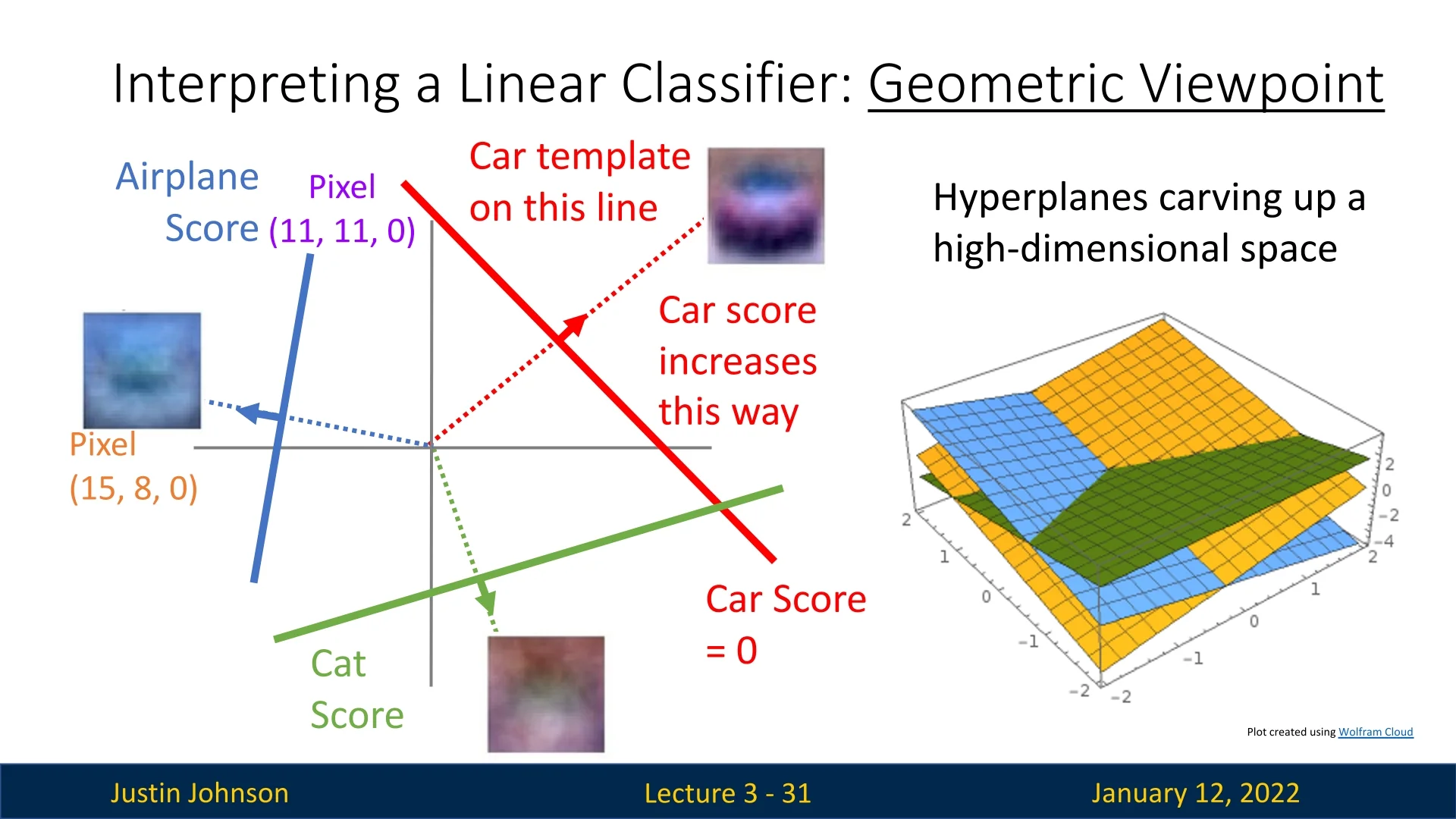
In Figure 3.10, the left side provides a simplified view after dimensionality reduction, while the right shows hyperplanes in the full space. These hyperplanes represent the boundaries where the classifier transitions between classes.
3.4.2 Limitations of Linear Classifiers
The geometric viewpoint highlights scenarios where linear classifiers fail.
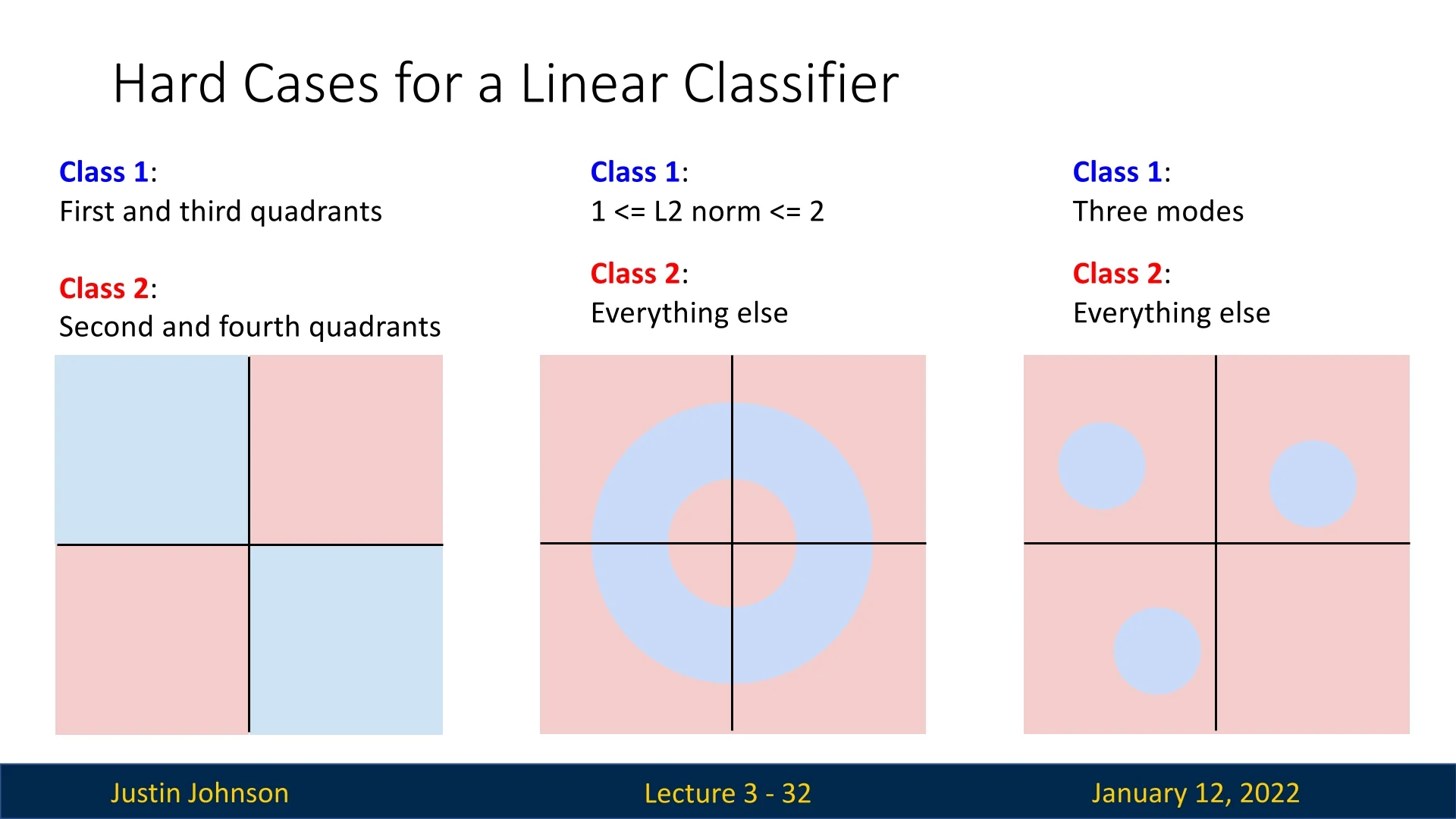
Left: Non-Linearly Separable Classes In this example, two classes occupy alternating quadrants. A single hyperplane cannot separate these regions, making the data not linearly separable.
Center: Nested Classes Here, one class forms a circular region inside another. The boundary between the two classes is inherently non-linear, so no hyperplane can effectively separate them.
Right: Multi-Modal Classes A single class consists of disjoint regions in the space, corresponding to multiple modes (e.g., variations in pose or orientation). Linear classifiers cannot handle such complexities because they only define a single hyperplane per class.
3.4.3 Historical Context: The Perceptron and XOR Limitation
Linear classifiers were among the first machine learning models introduced. The perceptron, developed in the late 1950s, was a milestone in artificial intelligence. However, its inability to handle the XOR function demonstrated the limitations of linear classifiers.
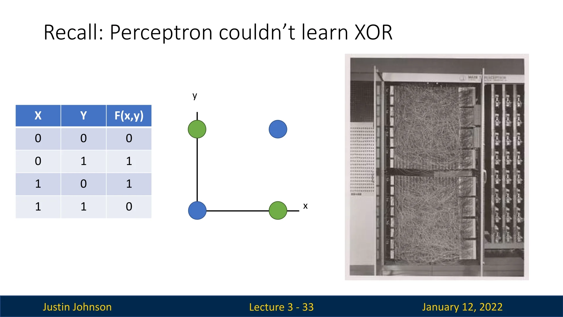
As shown in Figure 3.12, the XOR function has two regions (blue and green) that cannot be separated by a single linear boundary. This limitation highlighted the need for more powerful tools, eventually leading to the development of neural networks. Unlike linear classifiers, neural networks can represent non-linear decision boundaries, generalize well to unseen data, and perform efficient inference.
3.4.4 Challenges of High-Dimensional Geometry
Although this viewpoint provides valuable insights, it has limitations:
- Human Intuition Fails: Geometry behaves differently in high-dimensional spaces, often defying our intuition based on 2D/3D experiences.
- Linear Limitations: Linear classifiers rely on single hyperplanes, which are inadequate for handling non-linear or complex data distributions.
Despite these challenges, the geometric viewpoint lays the foundation for understanding why more advanced models, such as neural networks, are necessary. Neural networks overcome these issues by learning non-linear decision boundaries, a topic we will explore later.
3.5 Summary: Shortcomings of Linear Classifiers
Linear classifiers, while foundational, exhibit several limitations that are evident through different viewpoints (Figure 3.11).
3.5.1 Algebraic Viewpoint
Linear classifiers rely on the weighted sum of input features. Without non-linear transformations, they:
- Cannot model non-linear decision boundaries.
- Are limited in their expressiveness when classes are not linearly separable.
3.5.2 Visual Viewpoint
Visualizing the rows of the weight matrix as templates reveals:
- Templates depend heavily on backgrounds, leading to misclassifications (e.g., ships in non-ocean scenes).
- Multiple modes within a class (e.g., cars of different colors or orientations) cannot be represented by a single template.
3.5.3 Geometric Viewpoint
Interpreting data as points in high-dimensional space highlights:
- Linear classifiers fail when class distributions are not linearly separable (e.g., XOR configuration).
- Disjoint or nested regions within a class cannot be handled by a single hyperplane.
3.5.4 Conclusion: Linear Classifiers Aren’t Enough
These limitations necessitate more advanced models capable of non-linear decision boundaries and hierarchical feature learning, which we explore in subsequent chapters.
3.5.5 Choosing the Weights for Linear Classifiers
To effectively use linear classifiers, we must find a weight matrix \(W\) and bias vector \(\mathbf {b}\) that minimize misclassification. This involves two core tasks:
- Defining a loss function to quantify how good a choice of \(W\) is.
- Optimizing \(W\) to minimize the loss function.
In the rest of this chapter, we focus on the first task—choosing an appropriate loss function—while optimization will be addressed in the next chapter.
3.6 Loss Functions
Loss functions are fundamental to machine learning—they provide a scalar measure of how far a model’s predictions deviate from the true targets. Learning proceeds by minimizing this loss across a dataset, typically using gradient-based optimization.
Given a dataset with \(N\) examples, the total loss is computed as: \[ L = \frac {1}{N} \sum _{i=1}^{N} L_i(f(x_i, W), y_i), \] where:
- \(x_i\) is an input example.
- \(y_i\) is the corresponding true label.
- \(f(x_i, W)\) is the model’s prediction given parameters \(W\).
- \(L_i\) is the loss incurred on a single example.
3.6.1 Core Requirements for Loss Functions
Regardless of the task, certain properties are essential for a loss function to be useful in optimization:
- Differentiability: The loss should be differentiable with respect to the model parameters to enable the use of gradient-based optimization algorithms such as stochastic gradient descent (SGD).
- Monotonicity: The loss should increase as the model’s predictions become worse. That is, the loss should provide a signal that correlates with how ”wrong” a prediction is.
- Continuity: Smoothness in the loss landscape helps ensure stable updates during training and prevents erratic gradient jumps.
- Well-defined domain and range: The loss function should handle valid model outputs and targets gracefully and return real-valued, finite outputs.
3.6.2 Desirable Properties (Depending on the Task)
Beyond the core requirements, some properties may be beneficial or even necessary depending on the specific problem, model, or dataset:
- Convexity (for simpler models): Convex loss functions are easier to optimize because any local minimum is also a global minimum. While deep networks make the full objective non-convex, convex losses simplify training in linear models.
- Robustness to outliers: In tasks where noisy or mislabeled data is common, a loss function that does not over-penalize extreme errors (e.g., using absolute error instead of squared error) can improve generalization.
- Probabilistic or geometric interpretation: Some loss functions correspond to likelihood maximization under a specific model or enforce geometric margins. These interpretations often guide their design and applicability.
- Alignment with evaluation metrics: Ideally, the loss should correlate with the metric we care about at test time (e.g., accuracy, F1 score, BLEU). While exact alignment is not always feasible, closer alignment often leads to better results.
With these principles in mind, we now turn to specific loss functions commonly used in classification and regression tasks, beginning with one of the most widely used: the cross-entropy loss.
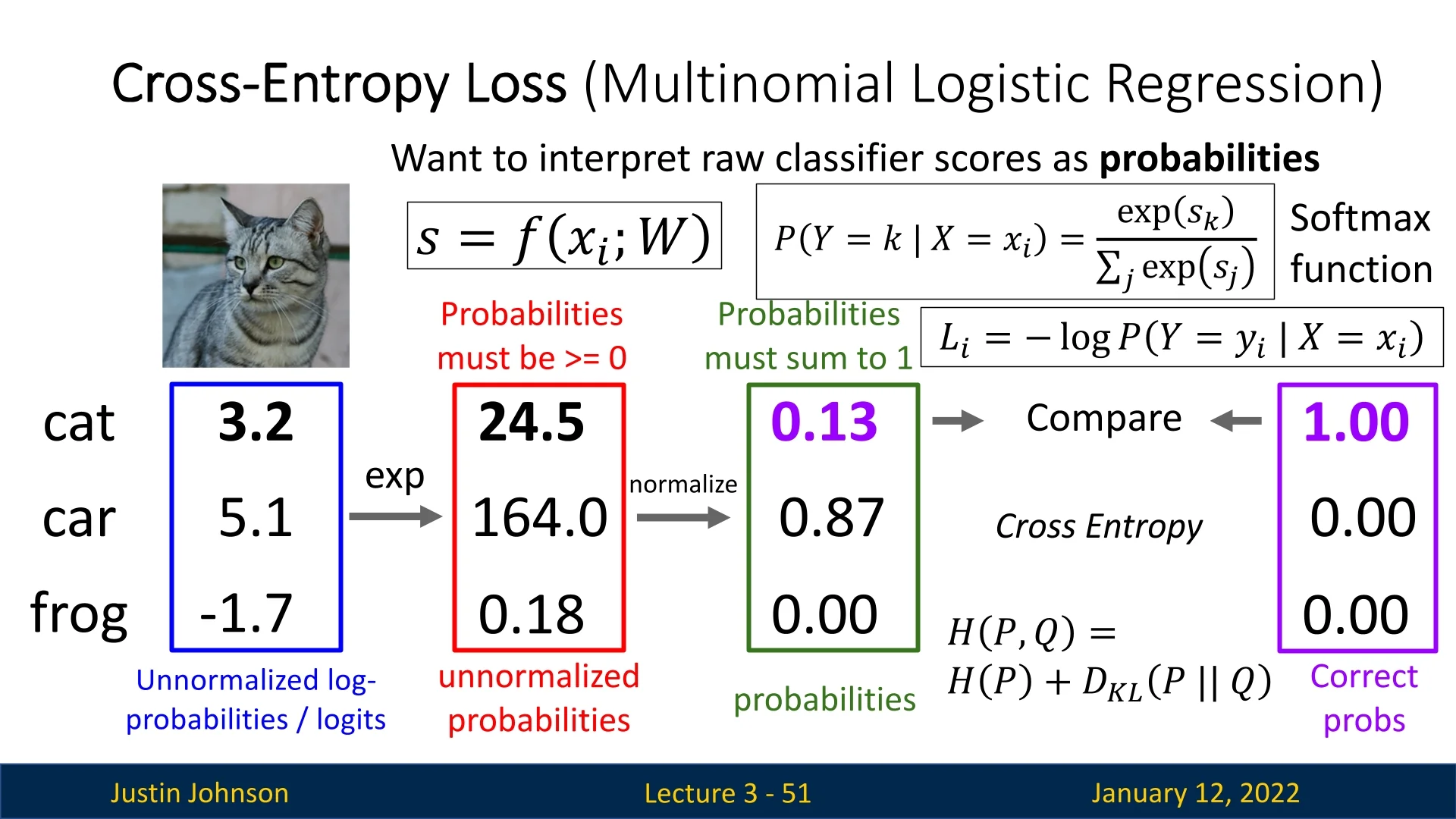
3.6.3 Cross-Entropy Loss
The cross-entropy loss, often used with the softmax function, provides a probabilistic interpretation of the classifier’s raw scores. For a single input \(x_i\) and weight matrix \(W\), the raw scores for each class are given by: \[ s_j = f(x_i, W)_j, \] where \(s_j\) represents the score for class \(j\). These scores are unnormalized, and their magnitude or sign has no direct probabilistic interpretation.
Softmax Function
The softmax function transforms raw class scores \(\{s_j\}\) into normalized probabilities \(\{p_j\}\), ensuring that \(\sum _j p_j = 1\) and \(p_j \ge 0\). Concretely: \[ p_j = \frac {e^{s_j}}{\sum _{k} e^{s_k}}, \] where:
- \(e^{s_j}\) is the exponentiated score for class \(j\).
- \(\sum _{k} e^{s_k}\) sums these exponentiated values across all classes, serving as a normalization factor.
A large score \(s_j\) results in a disproportionately large exponent \(e^{s_j}\), making \(p_j\) close to 1 while other probabilities remain small.
Advanced Note: Boltzmann Perspective. Softmax closely resembles a Boltzmann (Gibbs) distribution: each class’s weight is \(\exp (s_j)\), normalized so that \(\sum _j p_j = 1\). Although any mapping that yields a valid probability distribution could be used, softmax is especially attractive because, in tandem with cross-entropy, the derivative of the loss with respect to each logit \(s_j\) collapses to \((p_j - y_j)\). This concise gradient form is both straightforward to implement and numerically stable, simplifying training for classification tasks.
Loss Computation
The cross-entropy loss for a single example compares the predicted probability \(p_{y_i}\) of the correct class \(y_i\) with the true label: \[ L_i = -\log (p_{y_i}), \] where \(p_{y_i}\) is the softmax probability for the correct class. This loss penalizes the model heavily if the predicted probability for the correct class is small.
Example: CIFAR-10 Image Classification Consider a CIFAR-10 image (e.g., a cat) with three possible classes: cat (\(s_\mbox{cat} = 3.2\)), car (\(s_\mbox{car} = 5.1\)), and frog (\(s_\mbox{frog} = -1.7\)). Using the softmax function:
- 1.
- Compute \(e^{s_\mbox{cat}}, e^{s_\mbox{car}}, e^{s_\mbox{frog}}\).
- 2.
- Normalize by summing over all exponentiated scores.
- 3.
- Calculate the probability for the cat class, \(p_\mbox{cat}\), and compute the loss: \[ L_i = -\log (p_\mbox{cat}). \]
Properties of Cross-Entropy Loss
- Minimum Loss: The loss is \(0\) when \(p_{y_i} = 1\), meaning the model predicts the correct class with absolute confidence.
- Maximum Loss: The loss approaches \(+\infty \) as \(p_{y_i} \to 0\), heavily penalizing incorrect predictions.
- Initialization Insight: At random initialization, the raw scores \(s_j\) are small random values. Probabilities become uniform over \(C\) classes: \[ p_j = \frac {1}{C}. \] The loss becomes: \[ L_i \approx -\log \left (\frac {1}{C}\right ). \] This insight is useful for debugging model implementations.
Why These Names: Cross-Entropy and Softmax
The terms cross-entropy and softmax both arise from their mathematical origins in information theory and optimization. Understanding their names clarifies how they work together to form the standard probabilistic loss for classification.
Cross-Entropy: Encoding One Distribution Using Another The word cross-entropy comes from information theory, where it measures how “inefficient” it is to encode data from one probability distribution using another. Formally, for a true distribution \(p\) and a model prediction \(q\), \[ H(p,q) = -\sum _k p(k)\,\log q(k). \] The prefix “cross” reflects that the measure crosses the true data distribution \(p\) with the model’s predicted probabilities \(q\): the expectations are taken under \(p\), but the code lengths come from \(q\).
In classification, the true label is represented by a one-hot vector, so only the correct class \(y\) contributes: \[ H(p,q) = -\log q(y). \] This simplifies the cross-entropy loss to the negative log-likelihood (NLL) of the true class: minimizing it is equivalent to maximizing the probability assigned to the correct label. It penalizes confident wrong predictions heavily, guiding the model to output calibrated probabilities.
Softmax: Temperature and the Degree of “Softness” The softmax function transforms raw logits into probabilities through a temperature-controlled exponential normalization: \[ \sigma (z)_k = \frac {e^{z_k / \tau }}{\sum _j e^{z_j / \tau }}, \] where \(\tau > 0\) is the temperature parameter. This parameter directly determines how “soft” or “peaked” the resulting probability distribution is.
Role of the Temperature Parameter The temperature \(\tau \) modulates the confidence level of the model’s output:
- When \(\tau \to 0\), the exponentiation strongly amplifies logit differences, making one class dominate—producing an almost one-hot vector (a “hard” \(\arg \max \)).
- When \(\tau \to \infty \), the exponentials flatten out, assigning nearly equal probability to all classes—a uniform distribution.
- When \(\tau = 1\), the scale of logits is preserved, and this is the standard setting used in most classification networks.
Why \(\tau = 1\) by Default In most training settings, logits are unconstrained and naturally learn an appropriate scale through gradient descent. Setting \(\tau = 1\) keeps the mapping numerically stable while maintaining an interpretable balance between confidence and uncertainty. If \(\tau \) were much smaller, gradients could vanish due to overconfident probabilities; if much larger, predictions would be too smooth to separate classes effectively. Thus, \(\tau = 1\) provides a well-behaved trade-off between expressiveness and stability.
When and Why Temperature Is Changed Although \(\tau = 1\) is used during training, modifying it can serve specific purposes:
- Knowledge distillation. A higher temperature (\(\tau > 1\)) is used to soften the teacher’s output distribution, exposing relative confidence between classes and providing richer learning signals for the student network [228].
- Calibration and uncertainty estimation. At inference, temperature scaling can be applied to better align predicted probabilities with observed accuracies [202]. The optimal \(\tau \) is usually determined by minimizing negative log-likelihood on a validation set.
- Contrastive and self-supervised learning. In losses such as InfoNCE or CLIP’s contrastive loss, \(\tau \) controls embedding sharpness: smaller values increase separation between positives and negatives, while larger ones encourage smoother similarities.
Enrichment 3.6.3.1: Why Cross-Entropy Uses Logarithms, Not Squared Errors
CE loss is the standard choice for classification, especially when used with the softmax output layer. But why does it use logarithms, and not something simpler like squared error?
- (1) Mean Squared Error (MSE) used as a loss for classification: \[ \mbox{Loss} = \sum _j (p_j - \hat {p}_j)^2, \] where \( p \) is the one-hot target and \( \hat {p} \) is the predicted probability vector.
- (2) Replacing exponentials in softmax with squared values: \[ \mbox{Alternative softmax:} \quad \hat {p}_j = \frac {z_j^2}{\sum _k z_k^2}, \] which preserves normalization but alters the probabilistic and geometric behavior.
We now explain why both of these alternatives are inferior to cross-entropy loss with standard softmax.
1. Cross-entropy arises naturally from log-likelihood and KL divergence.
Cross-entropy loss is not an arbitrary design—it is grounded in the principle of maximum likelihood estimation (MLE) for categorical variables. Suppose the true class is \( y \), and the model assigns it predicted probability \( \hat {p}_y \). Then, under a categorical distribution, the log-likelihood is: \[ \log p(y \mid x) = \log \hat {p}_y, \] and the corresponding loss is the negative log-likelihood: \[ \mbox{Loss} = -\log \hat {p}_y. \] This expression generalizes to the full cross-entropy between the true label distribution \( p \) (which is typically one-hot) and the predicted probability vector \( \hat {p} \): \[ H(p, \hat {p}) = -\sum _j p_j \log \hat {p}_j. \]
More fundamentally, this quantity appears inside the Kullback–Leibler (KL) divergence, which measures how far a predicted distribution \( \hat {p} \) is from the true distribution \( p \): \[ \mbox{KL}(p \,\|\, \hat {p}) = \sum _j p_j \log \frac {p_j}{\hat {p}_j} = H(p, \hat {p}) - H(p). \]
Since \( H(p) \), the entropy of the true distribution, is fixed (independent of model parameters), minimizing the cross-entropy is equivalent to minimizing KL divergence.
Why is this useful? KL divergence is a principled and well-understood measure of distributional mismatch. By minimizing it, we are not just guessing the correct class—we are learning to approximate the entire target distribution. This ensures:
- Probabilistic correctness: The model assigns high probability to the true class while properly normalizing over alternatives.
- Meaningful confidence: The output reflects calibrated uncertainty, not just a one-hot choice.
- Gradient quality: The loss provides rich feedback even when the prediction is wrong, making learning faster and more stable.
Thus, cross-entropy’s link to likelihood and KL divergence ensures it is not only mathematically justified but also practically effective for probabilistic classification.
2. Squared error is poorly aligned with classification objectives.
Using mean squared error (MSE) for classification tasks is both conceptually inappropriate and mathematically inefficient. MSE assumes that outputs are continuous and independent, which does not hold in categorical prediction settings.
-
Lack of asymmetry:
The MSE loss penalizes the squared difference between the predicted probability vector \( \hat {p} \) and the one-hot encoded true label \( p \). The loss is defined as: \[ \mbox{MSE}(p, \hat {p}) = \sum _j (p_j - \hat {p}_j)^2. \]
This loss is symmetric: overestimating or underestimating the correct class by the same amount yields the same penalty. For instance, suppose the true class is class 1. Then: \[ (1 - 0.8)^2 = (1 - 1.2)^2 = 0.04. \]
In both cases, MSE assigns the same loss—even though the first prediction is underconfident, while the second is overconfident and invalid (e.g., \(\hat {p}_1 = 1.2\) is not even a valid probability). This symmetry fails to reflect the inherently asymmetric nature of classification, where confident wrong predictions are more damaging than slightly uncertain correct ones.
-
Weak penalty for confident errors:
MSE penalizes prediction errors quadratically but lacks the steep, exponential-like penalties needed for classification. Consider predicting a low probability for the true class: \[ \mbox{Cross-entropy:} \quad -\log (0.01) \approx 4.6 \] \[ \mbox{MSE:} \quad (1 - 0.01)^2 = 0.9801. \]
Cross-entropy provides a much sharper penalty for this confident error, which encourages the model to avoid placing extremely low probabilities on the correct class. This steepness acts like a strong corrective force during learning.
-
Poor gradient behavior:
While mean squared error (MSE) and cross-entropy (CE) losses may appear similar when applied directly to predicted probabilities, their gradients behave very differently once we consider how they flow through the softmax function during backpropagation.
Let’s assume the model outputs logits \( z_j \), which are passed through softmax: \[ \hat {p}_j = \frac {e^{z_j}}{\sum _k e^{z_k}}, \] to produce class probabilities.
Cross-entropy loss: \[ \mathcal {L}_{\mbox{CE}} = -\sum _j p_j \log \hat {p}_j. \] When computing the gradient of CE with respect to logits \( z_j \), we obtain a remarkably simple and well-behaved form: \[ \frac {\partial \mathcal {L}_{\mbox{CE}}}{\partial z_j} = \hat {p}_j - p_j. \] This gradient is linear in the prediction error and provides a clean, direct learning signal—especially effective when the model is confidently wrong (e.g., when \( \hat {p}_y \approx 0 \), the loss and gradient are large).
Mean squared error: \[ \mathcal {L}_{\mbox{MSE}} = \sum _j (\hat {p}_j - p_j)^2. \] The gradient with respect to the predicted probabilities is: \[ \frac {\partial \mathcal {L}_{\mbox{MSE}}}{\partial \hat {p}_j} = 2(\hat {p}_j - p_j), \] which appears similar to CE (up to a constant factor). However, when we backpropagate through the softmax, the full gradient with respect to the logits \( z_j \) becomes: \[ \frac {\partial \mathcal {L}_{\mbox{MSE}}}{\partial z_j} = 2 \sum _k (\hat {p}_k - p_k)\hat {p}_k(\delta _{jk} - \hat {p}_j), \] which is more complex and involves interactions across all classes. This entangled gradient signal is harder to interpret and can lead to slower, less stable learning.
Key distinction: Cross-entropy provides a local gradient per logit that depends only on the predicted probability and the true label. MSE, in contrast, introduces non-local coupling between logits due to the softmax Jacobian. As a result, cross-entropy produces sharper corrections, especially when the model is confidently incorrect, while MSE gradients may become weak or noisy in such regimes.
Conclusion: Although the MSE and CE gradients appear similar at the output layer, their behavior through the softmax transformation differs significantly. Cross-entropy leads to more effective training dynamics, which is one reason it is the preferred loss for classification tasks.
-
Mismatch with softmax structure:
MSE assumes the outputs \( \hat {p}_j \) are independent scalar predictions that can be pushed toward 0 or 1 freely. But softmax outputs are constrained: \[ \sum _j \hat {p}_j = 1, \quad \hat {p}_j \in (0,1). \]
This means increasing one class’s probability forces other probabilities to decrease. MSE ignores this coupling, treating each component separately. As a result, MSE fails to exploit the inter-class competition inherent to classification, and its gradients don’t reflect how increasing confidence in one class affects others.
In contrast, cross-entropy is designed specifically for probability distributions. It takes into account the full predicted vector and compares it to the one-hot true label in a principled, probabilistic manner.
3. Using \( z_j^2 / \sum _k z_k^2 \) instead of softmax breaks probabilistic structure.
Some have proposed using squared logits in place of exponentials to define a normalized output: \[ \hat {p}_j = \frac {z_j^2}{\sum _k z_k^2}. \] While this guarantees outputs in \([0,1]\) that sum to 1, it fails in several key ways:
- No log-likelihood interpretation: This function does not arise from any known probabilistic model. There’s no equivalent of a negative log-likelihood or KL divergence for guiding learning.
- Limited expressiveness: The squaring operation is symmetric around 0, so it cannot distinguish between positive and negative evidence. For example, \( z_j = -5 \) and \( z_j = 5 \) produce the same result.
- Unstable or flat gradients: Near-zero logits yield gradients close to zero, which can stall learning. Exponentials in softmax, by contrast, ensure that even small logit differences yield sharp probability contrasts, especially early in training.
- No exponential separation of scores: Softmax amplifies differences exponentially, creating a margin-like separation between classes. This is essential for learning sharp decisions in high-dimensional settings; \( z^2 \) lacks this behavior.
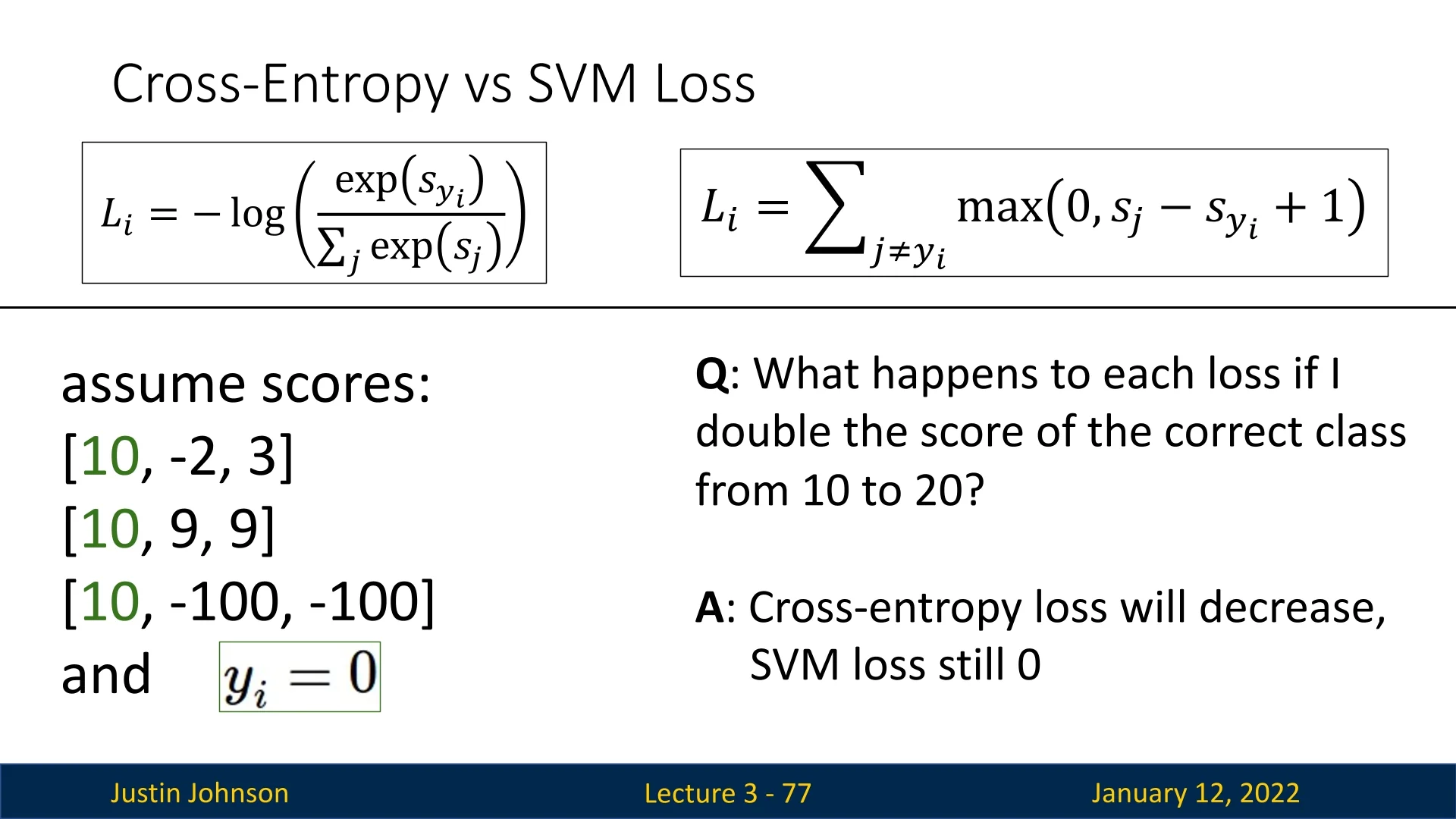
3.6.4 Multiclass SVM Loss
The multiclass SVM loss, also known as the hinge loss (so named because its graphical shape resembles a door hinge), is a straightforward yet powerful loss function. Its goal is to ensure that the score of the correct class is higher than all other class scores by at least a predefined margin \(\Delta \). If this condition is satisfied, the loss is 0; otherwise, the loss increases linearly with the violation.
Loss Definition
For a single training example \((x_i, y_i)\), the multiclass SVM loss is defined as: \[ L_i = \sum _{j \neq y_i} \max (0, s_j - s_{y_i} + \Delta ), \] where:
- \(s_j = f(x_i, W)_j\): the score for class \(j\),
- \(s_{y_i}\): the score for the correct class,
- \(\Delta \): the margin, typically set to \(1\).
The total loss across the dataset is the average of individual losses: \[ L = \frac {1}{N} \sum _{i=1}^{N} L_i. \]
Example Computation
Let us compute the multiclass SVM loss for a small dataset containing three images (a cat, a car, and a frog) from CIFAR-10. The model outputs the following scores for these images across three classes (cat, car, frog):
\[ \begin {aligned} \mbox{Cat Image Scores:} & \quad (s_\mbox{cat}, s_\mbox{car}, s_\mbox{frog}) = (3.2, 5.1, -1.7), \\ \mbox{Car Image Scores:} & \quad (s_\mbox{cat}, s_\mbox{car}, s_\mbox{frog}) = (1.3, 4.9, 2.0), \\ \mbox{Frog Image Scores:} & \quad (s_\mbox{cat}, s_\mbox{car}, s_\mbox{frog}) = (2.2, 2.5, -3.1). \end {aligned} \]
Loss for the Cat Image The true class is ”cat.” The loss is computed as: \[ L_\mbox{cat} = \max (0, s_\mbox{car} - s_\mbox{cat} + 1) + \max (0, s_\mbox{frog} - s_\mbox{cat} + 1), \] \[ L_\mbox{cat} = \max (0, 5.1 - 3.2 + 1) + \max (0, -1.7 - 3.2 + 1), \] \[ L_\mbox{cat} = 2.9. \]
Loss for the Car Image The true class is ”car.” The loss is: \[ L_\mbox{car} = \max (0, s_\mbox{cat} - s_\mbox{car} + 1) + \max (0, s_\mbox{frog} - s_\mbox{car} + 1), \] \[ L_\mbox{car} = \max (0, 1.3 - 4.9 + 1) + \max (0, 2.0 - 4.9 + 1), \] \[ L_\mbox{car} = 0. \]
Loss for the Frog Image The true class is ”frog.” The loss is: \[ L_\mbox{frog} = \max (0, s_\mbox{cat} - s_\mbox{frog} + 1) + \max (0, s_\mbox{car} - s_\mbox{frog} + 1), \] \[ L_\mbox{frog} = \max (0, 2.2 - (-3.1) + 1) + \max (0, 2.5 - (-3.1) + 1), \] \[ L_\mbox{frog} = 12.9. \]
Total Loss The total loss across the dataset is the average of individual losses: \(L = \frac {1}{3} (L_\mbox{cat} + L_\mbox{car} + L_\mbox{frog}) = \frac {1}{3} (2.9 + 0 + 12.9) = 5.27.\)
Key Questions and Insights
- What happens if the loss sums over all classes, including the correct class? In this case, all scores would inflate uniformly, adding an extra constant (approx. the predetermined margin) to the loss. This does not change the model’s preferences over the weight matrix \(W\).
- What if we use a mean instead of a sum for the loss? The loss values are scaled by a factor of \((1 / C-1)\), where \(C\) is the number of classes. The model’s behavior remains unaffected.
- What if we square the loss terms? Squaring would alter the loss function’s sensitivity to large deviations, changing the behavior and preferences over \(W\).
- Is the weight matrix \(W\) unique when the loss is zero? No, scaling \(W\) (e.g., multiplying it by 2) maintains zero loss because the margin condition is still satisfied. Regularization, which we’ll later discuss thoroughly, helps select a preferred \(W\).
3.6.5 Comparison of Cross-Entropy and Multiclass SVM Losses
Both losses aim to guide the model toward correct predictions, but their behavior differs significantly:
- Score Sensitivity: The SVM loss becomes invariant once the margin condition is satisfied, while the cross-entropy loss continues to decrease as the correct class score increases.
- Probabilistic Interpretation: The cross-entropy loss provides a natural probabilistic interpretation of predictions, whereas the SVM loss focuses on maintaining a margin.
- Scaling Effects: Scaling scores affects the cross-entropy loss but not the SVM loss, highlighting the need for regularization in SVM-based models.
Debugging with Initial Loss Values
An effective way to verify whether a model is configured correctly is to examine the loss value at the very start of training, before any updates have been applied. For both cross-entropy and margin-based losses (e.g., SVM), there are mathematically predictable loss values when the model begins with random, unbiased weights.
Cross-Entropy Loss: Expected Initial Value.
Suppose a classifier is initialized such that it produces uniform predictions over all \(C\) classes (as is often the case with random initialization and symmetric weight distributions). That is, the model assigns each class probability: \[ \hat {p}_j = \frac {1}{C}. \] The cross-entropy loss for a one-hot label \(p_j = \delta _{jy}\) becomes: \[ \mathcal {L}_{\mbox{CE}} = -\sum _j p_j \log \hat {p}_j = -\log \hat {p}_y = -\log \frac {1}{C} = \log C. \] So at initialization, we expect the cross-entropy loss to be approximately \( \log C \). For example: \[ C = 10 \quad \Rightarrow \quad \mathcal {L}_{\mbox{CE}} \approx \log 10 \approx 2.3. \]
SVM (Hinge) Loss: Expected Initial Value.
For the multiclass SVM or hinge loss (often used in margin-based classifiers), the typical loss formulation is: \[ \mathcal {L}_{\mbox{SVM}} = \sum _{j \neq y} \max (0, f_j - f_y + 1), \] where \(f_j\) is the score (logit) for class \(j\), and \(y\) is the true class.
If the scores \(f_j\) are initialized to be equal or nearly equal (as in uniform random initialization), then: \[ f_j \approx f_y \quad \Rightarrow \quad f_j - f_y + 1 \approx 1 \mbox{ for all } j \neq y. \] This means the max terms are all active, and the total loss becomes: \[ \mathcal {L}_{\mbox{SVM}} \approx \sum _{j \neq y} 1 = C - 1. \] So at initialization, we expect the hinge loss to be approximately \(C - 1\). For example: \[ C = 10 \quad \Rightarrow \quad \mathcal {L}_{\mbox{SVM}} \approx 9. \]
How This Helps Debugging?
Inspecting the initial loss is a fast and effective sanity check. It helps confirm that the model, label encoding, output activations, and loss function are correctly configured—before any training begins. While this section focuses on cross-entropy and hinge losses, the principle extends to many loss functions in both classification and regression.
- If the loss is too low at initialization: This may signal data leakage (e.g., label information leaking into the inputs), incorrect use of pretrained weights, or even a flaw in the loss implementation. For example, a cross-entropy loss close to zero implies that the model is already assigning very high probability to the correct class—unlikely if the weights are truly untrained.
- If the loss is too high: This might indicate degenerate model outputs (e.g., extremely large or small logits), incorrect label encoding (such as using class indices instead of one-hot vectors), or numerical instability. In CE, large logit magnitudes with wrong signs can spike the loss well above \( \log C \).
- If the loss deviates significantly from the expected baseline (e.g., \( \log C \) for cross-entropy or \( C - 1 \) for SVM): This may reflect label mismatches, class imbalance, or improperly scaled outputs (e.g., skipping softmax or applying wrong activation functions).
In short: Mismatch with expected baseline (e.g., \( \log C \) for CE or \( C - 1 \) for SVM) suggests issues like misaligned labels, class imbalance, or broken forward pass logic. Checking the initial loss should be a routine step when setting up models. It helps catch configuration bugs early—often before training even begins.
Conclusion: SVM, Cross Entropy, and the Evolving Landscape of Loss Functions
- SVM Loss: Suitable for margin-based classification but requires regularization to handle multiple solutions with zero loss.
- Cross-Entropy Loss: Ideal for probabilistic interpretation and gradient-based optimization, often preferred in deep learning models.
Both losses have unique advantages, and the choice depends on the application and desired behavior during training.
Enrichment 3.6.6: Additive Margin Softmax (AM-Softmax)
Motivation
From Separability to True Discriminability In many high-dimensional recognition tasks—such as face verification, speaker recognition, and product retrieval—standard softmax cross-entropy loss ensures only that the correct class logit exceeds the others. While this suffices for separability, it does not guarantee discriminability: features of the same class may be loosely scattered, and different classes may overlap in feature space. To achieve robust, generalizable embeddings, one seeks compact intra-class clusters and large inter-class margins.
Angular Formulation on the Hypersphere A practical approach to achieve this geometric interpretability is to reformulate the decision boundary in angular terms. Let the feature vector \(x \in \mathbb {R}^D\) and class prototype \(w_j \in \mathbb {R}^D\) represent, respectively, the sample and the \(j\)-th class weight. Both are \(\ell _2\)-normalized onto the unit hypersphere: \[ \tilde {x} = \frac {x}{\|x\|_2}, \qquad \tilde {w}_j = \frac {w_j}{\|w_j\|_2}. \] The cosine similarity between them defines the logit: \begin {equation} z_j = s\,\tilde {w}_j^{\top }\tilde {x} = s\,\cos \theta _j, \qquad \theta _j \in [0^\circ ,180^\circ ], \label {eq:chapter3_amsoftmax_cosine} \end {equation} where \(s > 0\) rescales logits for numerical stability and gradient control. Under this normalized form, decisions depend solely on the angular distance between feature and prototype—making \(\theta _j\) a natural measure of class alignment.
With conventional softmax applied to Eq. (3.1), the binary decision boundary is the angular bisector \(\cos \theta _1 = \cos \theta _2\). A sample infinitesimally closer to its true prototype is already deemed correct—offering no safety buffer. Thus arose the idea of introducing explicit angular margins.
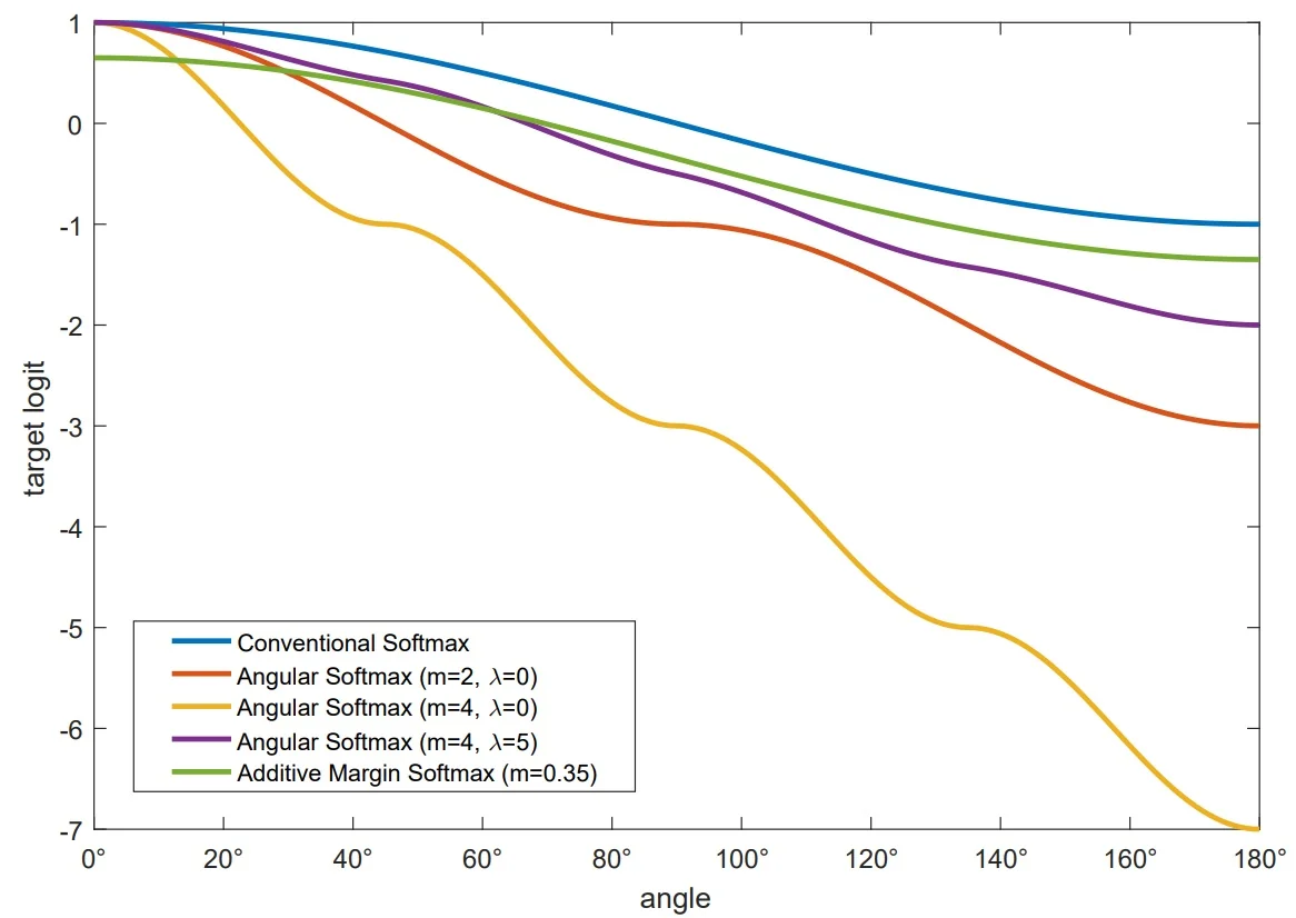
Historical Progress: Multiplicative Margins and Their Limitations Early works like L-Softmax [386] and A-Softmax (SphereFace) [387] pioneered margin-based formulations in angular space. SphereFace enforced a multiplicative constraint by replacing \(\cos \theta _y\) with \(\cos (m\theta _y)\) for integer \(m \ge 1\). This effectively narrowed the acceptance cone of the correct class, requiring samples to align more closely with their class prototype to be correctly classified.
However, \(\cos (m\theta )\) is non-monotonic on \([0, \pi ]\), oscillating across sectors and causing ambiguous gradients. SphereFace resolved this via a piecewise surrogate \[ \psi (\theta ) = (-1)^k\cos (m\theta ) - 2k, \quad \theta \in \big [\tfrac {k\pi }{m}, \tfrac {(k+1)\pi }{m}\big ], \] and an annealing blend \[ \psi _\lambda (\theta ) = \frac {\lambda \,\cos \theta + \psi (\theta )}{\lambda + 1}, \] which starts near \(\cos \theta \) (large \(\lambda \)) and transitions to \(\psi (\theta )\) (small \(\lambda \)). While conceptually elegant, this multiplicative margin had several drawbacks:
- Angle-dependent margin. The effective margin shrinks non-uniformly with \(\theta \), applying excessive pressure to hard samples but little to easy ones.
- Gradient instability. The piecewise function introduces kinks and steep, regime-dependent slopes, making optimization sensitive to initialization and learning rate.
- Hyperparameter burden. The integer \(m\), annealing schedule, and blending \(\lambda \) require manual tuning.
AM-Softmax (CosFace): The Additive Cosine Margin Solution AM-Softmax (CosFace) [678, 679] resolves two core issues of earlier margin losses. First, L-Softmax [386] and A-Softmax (SphereFace) [387] enforce margins by warping angles (e.g., \(\cos (m\theta _y)\)), which requires a piecewise surrogate to remain monotone and a careful annealing schedule for stability. Second, their angle-dependent pressure pushes hard samples far more than easy ones, yielding unbalanced gradients and inconsistent intra-class compactness. AM-Softmax instead applies a fixed additive margin in cosine space, keeping the target strictly monotone and the optimization simple.
Formulation (single change to the target logit). After \(\ell _2\)-normalizing features and weights, logits are \(z_j = s\,\cos \theta _j\). AM-Softmax modifies only the correct-class logit: \begin {equation} z_y^{\mbox{AM-Softmax}} = s\,(\cos \theta _y - m), \qquad z_j = s\,\cos \theta _j \ \ (j \neq y), \label {eq:chapter3_amsoftmax_main} \end {equation} with scale \(s>0\) and margin \(m>0\). In the binary normalized case, the decision boundary shifts from \(\cos \theta _1=\cos \theta _2\) to \begin {equation} \cos \theta _1 - m = \cos \theta _2 \quad \Longleftrightarrow \quad \cos \theta _1 - \cos \theta _2 = m, \label {eq:chapter3_amsoftmax_boundary_refined} \end {equation} so the target class must win by a fixed cosine gap \(m\)—independent of absolute angles.
Why AM-Softmax beats multiplicative/angle-space margins.
-
Smooth, bounded, and stable target. AM-Softmax defines its target logit as \[ z_y = s(\cos \theta _y - m), \qquad \frac {\partial z_y}{\partial \theta _y} = -s\sin \theta _y. \] This function is \(C^\infty \)-smooth, strictly decreasing, and globally bounded by \(|\partial z_y/\partial \theta _y| \le s\). Under cross-entropy, where \(\partial L/\partial z_y = p_y - 1\), we obtain \[ \Bigl |\frac {\partial L}{\partial \theta _y}\Bigr | = s|p_y - 1|\sin \theta _y \le s. \] This upper bound means that no matter how misaligned the feature is, the gradient magnitude never exceeds \(s\), giving a uniformly Lipschitz-continuous landscape—changes in angle produce proportionally limited changes in loss. In optimization terms, this limits gradient variance across the batch, keeping learning updates stable and predictable. At random initialization, when feature directions are nearly uniform on the hypersphere, \(\mathbb {E}[\sin ^2\theta _y] = \tfrac {1}{2}\), yielding a consistent average gradient scale of order \(\mathcal {O}(s)\). This steady “signal power” ensures smooth convergence without oscillations or exploding updates.
By contrast, multiplicative (angle-space) margins, such as SphereFace, approximate \(z_y \!\approx \! s\cos (m\theta _y)\). Their gradient, \[ \frac {\partial z_y}{\partial \theta _y} \!\approx \! -sm\sin (m\theta _y), \] is \(m\)-times steeper, oscillatory, and periodically reverses direction—creating “kinks” between angular sectors. Each kink acts as a sharp ridge in the loss surface, causing large, erratic gradient swings (\(\mbox{Var}[\partial z_y/\partial \theta _y]\!\propto \! m^2\)) and forcing the use of annealing schedules to gradually “turn on” the margin. AM-Softmax’s smoothness removes these discontinuities entirely, yielding a single well-behaved basin of descent.
Intuitively, AM-Softmax feels like descending a gentle, continuous slope—easy to control—whereas multiplicative margins resemble stepping down a jagged staircase with uneven steps. The smoother surface means more stable optimization, faster convergence, and far fewer tuning complications.
-
Uniform margin and geometric clarity. AM-Softmax applies a fixed additive margin in cosine space: \[ \cos \theta _y > \cos \theta _j + m \quad (\forall j \neq y), \] meaning the feature’s similarity to its true prototype must exceed that to every distractor by at least \(m\). This margin is absolute and identical for all samples, defining a uniform “safety gap” in cosine similarity.
To understand its effect, note that a “hard” distractor corresponds to a small angle \(\theta _j\) (the feature is near a wrong prototype), while an “easy” distractor has a large \(\theta _j\) (the feature is far from any confusion). The largest allowable deviation for the correct class before misclassification is \[ \theta _y^{\max } = \arccos (\cos \theta _j + m), \] so the decision boundary shifts inward by a fixed cosine offset \(m\). A small linearization gives \[ \Delta \theta _y \approx \frac {m}{\sin \theta _j}, \] which scales smoothly: when \(\theta _j\) is large (easy case), \(\sin \theta _j\!\approx \!1\), giving a mild tightening; when \(\theta _j\) is smaller (hard case), the pull is slightly stronger but never extreme.
In effect, AM-Softmax balances the forces applied to all samples—gently encouraging easy ones to refine alignment, while giving hard ones enough extra pull to escape confusion without destabilizing gradients.
-
Numerical illustration (AM \(m{=}0.35\) vs. A-Softmax \(m{=}4\)). Consider two distractors at different angular distances from the true prototype:
- Hard distractor: \(\theta _j = 60^\circ \) (\(\cos \theta _j = 0.5\)). AM-Softmax requires \(\cos \theta _y > 0.85 \Rightarrow \theta _y^{\max } \approx 31.8^\circ \), halving the decision cone—firm but reasonable separation. A-Softmax enforces \(\theta _y^{\max } = 60^\circ / 4 = 15^\circ \), a fourfold contraction that yields excessive gradient magnitude and slower convergence.
- Easy distractor: \(\theta _j = 90^\circ \) (\(\cos \theta _j = 0\)). AM-Softmax gives \(\theta _y^{\max } \approx 69.5^\circ \), applying only mild pressure to refine alignment. A-Softmax insists on \(22.5^\circ \), over-tightening already safe samples.
In both cases AM-Softmax uses the same additive gap (\(\Delta \cos = m = 0.35\)), yet its angular effect self-adjusts via the sphere’s curvature (\(\sin \theta _j\)): the pull is adaptive but bounded, preventing gradient imbalance across the batch.
Geometric intuition. On the hypersphere, AM-Softmax transforms the softmax bisector \(\cos \theta _1 = \cos \theta _2\) into a parallel offset \(\cos \theta _1 - \cos \theta _2 = m\). Each class thus gains a uniform spherical cap—a “moat” of cosine width \(m\)—that separates prototypes evenly. All classes retain equally sized, isotropic decision regions, while multiplicative margins distort these shapes, over-squeezing poles and stretching equators. The additive cosine rule therefore ensures fair, stable, and geometrically clean separation across the sphere.
Hyperparameters and practice.
- Scale \(s\). Acts as an inverse temperature that sharpens posteriors and scales gradients; typical settings range from \(s{=}30\) to \(s{=}64\) depending on batch size and dataset.
- Margin \(m\). Sets the required cosine lead; values in \(m\in [0.2, 0.5]\) are common. Larger \(m\) strengthens separation but can slow early convergence.
In large-scale face recognition, \((s,m)=(64,0.35)\) is a widely used, robust choice [679]. Compared to L-Softmax and SphereFace, AM-Softmax achieves stronger, more uniform discrimination with a simpler, more stable training recipe.
A-Softmax versus AM-Softmax at a glance A-Softmax (SphereFace) enforces a multiplicative, angle-dependent margin via a piecewise target \(\psi (\theta )\) and often requires a blending schedule \(\lambda \), which can yield uneven gradients and nontrivial hyperparameter tuning. AM-Softmax instead subtracts a fixed margin \(m\) in cosine space, producing a smooth, strictly monotone target and a uniform decision buffer with only two interpretable scalars \((s,m)\).
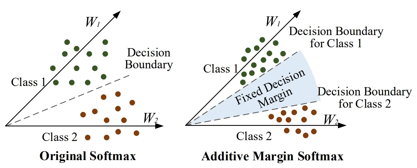
Why it helps and how it looks in feature space Training with normalized features and weights makes the classifier rotate features toward the correct prototype rather than inflate norms. AM-Softmax pushes the decision boundary inward by a constant buffer in cosine space; compared with the softmax bisector and multiplicative margins, this fixed-gap rule yields visibly tighter intra-class clusters and larger inter-class spacing, improving open-set identification and verification.
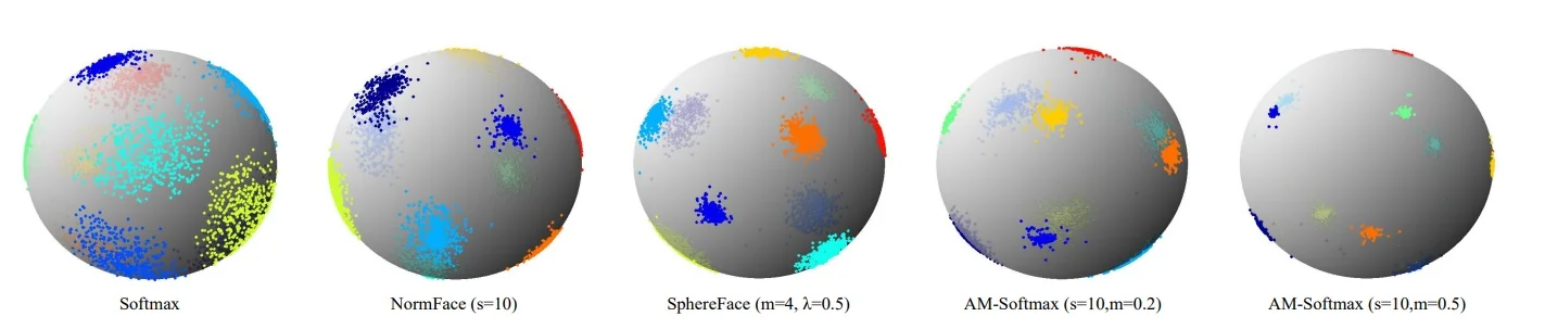
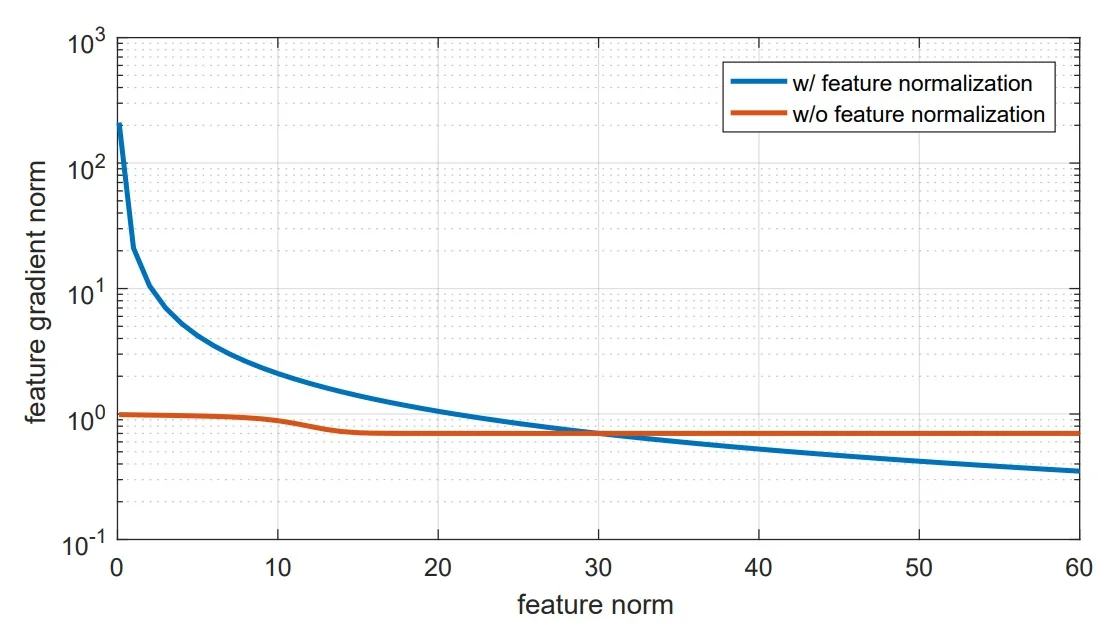
Gradient behavior and the role of normalization Hyperspherical normalization decouples gradient magnitude from raw feature norms: updates mainly rotate features toward \(\tilde {w}_y\) and away from impostors instead of amplifying vector lengths. The scale \(s\) sharpens the posterior and proportionally scales gradients—too large an \(s\) can reduce numerical slack. The empirical effect is visualized below.
# AM-Softmax forward (NumPy/PyTorch-like pseudocode)
# X: (N, D), W: (K, D), y: (N,), s: float, m: float
Xn = X / np.linalg.norm(X, axis=1, keepdims=True)        # (N, D) feature normalization
Wn = W / np.linalg.norm(W, axis=1, keepdims=True)        # (K, D) weight normalization
cos = Xn @ Wn.T                                          # (N, K) cosine similarities
logits = s * cos
idx = np.arange(X.shape[0])
logits[idx, y] = s * (cos[idx, y] - m)                   # subtract fixed margin on target
loss = cross_entropy(logits, y)                          # standard CE on modified logits
Experiments and ablations
Benchmarks and observations Across standard face recognition benchmarks—LFW, BLUFR, and MegaFace—AM-Softmax delivers consistent gains over plain softmax and comparable or better accuracy than A-Softmax, while being substantially easier to train. Moderate margins in the range \(m \in [0.30, 0.45]\) strike a practical balance: they create compact, well-separated embeddings without destabilizing optimization. Beyond this range, overly large margins can over-constrain the angular decision regions, leading to slower convergence or gradient saturation.
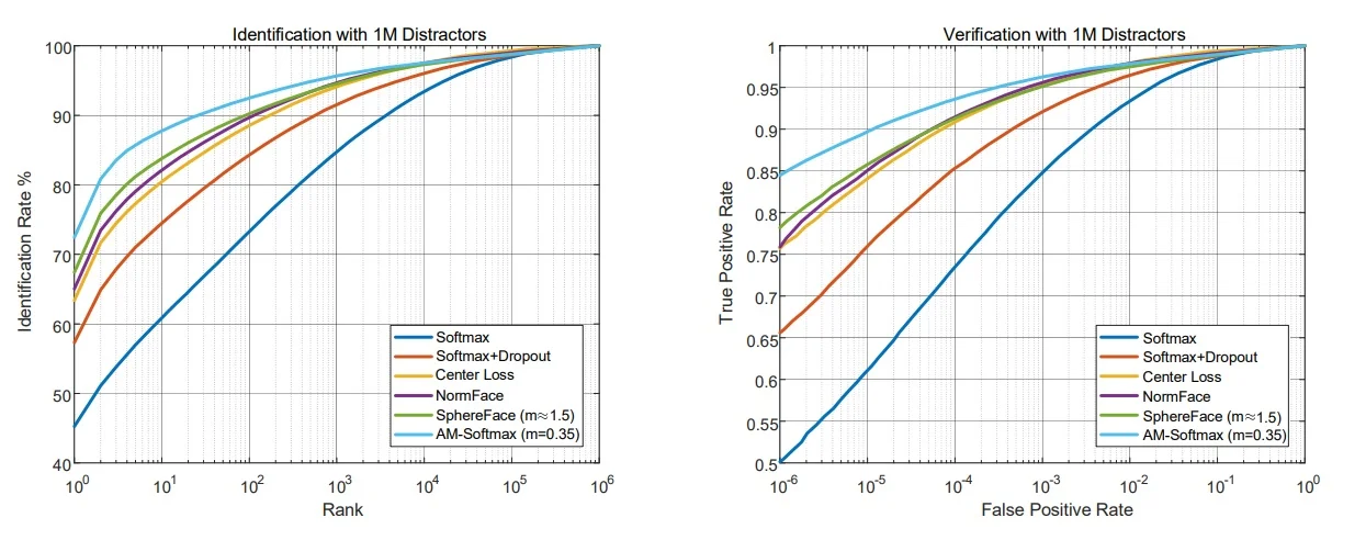
Results reported by [678] are summarized in the table below. Identification and verification results on MegaFace are additionally visualized using the Cumulative Match Characteristic (CMC) curve—a standard metric for large-scale identification. The CMC curve plots the probability that the correct identity appears within the top-\(k\) retrieved matches; a higher curve (especially at small ranks such as rank-1 or rank-5) indicates stronger discriminative power and better generalization under open-set conditions.
When comparing absolute performance numbers, note that differences in backbone architectures (e.g., ResNet-18 vs. ResNet-64) can affect reported accuracy. Nonetheless, AM-Softmax’s key advantage is practical: it achieves state-of-the-art discriminative embedding quality without requiring the delicate annealing schedules or piecewise margin surrogates needed by multiplicative-margin methods such as SphereFace.
| Loss | \(m\) | LFW 6k | BLUFR VR@0.01% | BLUFR VR@0.1% | MegaFace Rank1@1e6 | MegaFace VR@1e-6 |
|---|---|---|---|---|---|---|
| Softmax | - | 97.08% | 60.26% | 78.26% | 50.85% | 50.12% |
| Softmax + 75% dropout | - | 98.62% | 77.64% | 90.91% | 63.72% | 65.58% |
| Center Loss | - | 99.00% | 83.30% | 94.50% | 65.46% | 75.68% |
| NormFace | - | 98.98% | 88.15% | 96.16% | 75.22% | 75.88% |
| A-Softmax (SphereFace) | \(\sim \)1.5 | 99.08% | 91.26% | 97.06% | 81.93% | 78.19% |
| AM-Softmax | 0.25 | 99.13% | 91.97% | 97.13% | 81.42% | 83.01% |
| AM-Softmax | 0.30 | 99.08% | 93.18% | 97.56% | 84.02% | 83.29% |
| AM-Softmax | 0.35 | 98.98% | 93.51% | 97.69% | 84.82% | 84.44% |
| AM-Softmax | 0.40 | 99.17% | 93.60% | 97.71% | 84.51% | 83.50% |
| AM-Softmax | 0.45 | 99.03% | 93.44% | 97.60% | 84.59% | 83.00% |
| AM-Softmax | 0.50 | 99.10% | 92.33% | 97.28% | 83.38% | 82.49% |
| AM-Softmax w/o FN | 0.35 | 99.08% | 93.86% | 97.63% | 87.58% | 82.66% |
| AM-Softmax w/o FN | 0.40 | 99.12% | 94.48% | 97.96% | 87.31% | 83.11% |
| Setting | MegaFace Rank1 | MegaFace VR |
|---|---|---|
| AM-Softmax (No overlap removal) | 75.23% | 87.06% |
| AM-Softmax (Overlap removal) | 72.47% | 84.44% |
Where AM-Softmax helps, and where it does not
AM-Softmax is most effective when the deployment compares embeddings by cosine similarity; its fixed angular buffer shapes features into tight, well-separated cones that transfer directly to such back-ends.
- Open-set identification and verification. Tasks that reuse embeddings at inference (e.g., face recognition, speaker verification) benefit because AM-Softmax tightens intra-class cones and enlarges inter-class gaps on the unit hypersphere, improving cosine-based matching, reducing false matches under many distractors, and stabilizing verification thresholds.
-
Prototype or cosine back-ends. When inference compares a query embedding to stored class directions by cosine, AM-Softmax aligns training with the deployment rule and avoids train–test mismatch. Common patterns include.
- Prototype classifiers. Average support embeddings to form a class prototype and predict by highest cosine; AM-Softmax’s hyperspherical clustering makes prototypes representative and decision margins reliable.
- Cosine k-NN over a gallery. Retrieve by nearest neighbors in cosine space; tighter intra-class cones increase top-\(k\) recall and reduce impostor matches.
- Incremental or few-shot updates. Add new classes by storing one or a few prototypes without retraining the head; the fixed margin leaves “room” on the sphere so unseen prototypes separate cleanly from existing ones.
- Closed-set-only classification. If evaluation is pure argmax over the training label set and embeddings are never reused, a well-regularized cross-entropy baseline may match accuracy; AM-Softmax’s advantage primarily appears in cosine retrieval and verification.
- Hyperparameter sensitivity of \((s,m)\). An over-large margin \(m\) makes the target unattainable early and stalls learning, while an over-large scale \(s\) over-sharpens posteriors, amplifies gradients, and can destabilize optimization; prefer small, conservative adjustments around a solid default.
- Noisy labels or overlapping classes. A hard angular buffer over-penalizes ambiguous or mislabeled samples; prefer a smaller \(m\), sample reweighting, label smoothing, or data cleaning when noise is present.
- Class imbalance and small batches. Aggressively tightened cones can underfit minority classes when they are under-sampled; use class-balanced sampling, slightly smaller \(m\), or class-aware/adaptive margins.
- Domain shift and calibration. The cosine-margin objective optimizes discrimination on the source domain; probability calibration can degrade under shift, so apply post-hoc calibration (e.g., temperature scaling) on a target-domain validation set if downstream components consume probabilities.
- Beyond classification heads. AM-Softmax is designed for classifier embeddings and is not a drop-in objective for regression, dense prediction, or detection heads without additional architectural design.
- Normalization trade-offs. normalized features/weights slightly reduce the linear head’s flexibility; if deployment does not use cosine similarity, the geometric alignment benefit may be underutilized.
Practical notes on tuning \(s\) and \(m\)
- Roles. The margin \(m\) is a safety buffer in cosine space that sets the required lead of the correct class over impostors, while the scale \(s\) is an inverse temperature that sharpens posteriors and scales gradients.
- Starting grid. A compact, effective sweep is
\((s,m)\in \{16,30,64\}\times \{0.25,0.30,0.35,0.40,0.45\}\), with \((30,0.35)\) as a strong default. - Adjusting \(m\). If loss plateaus high or training accuracy stagnates, decrease \(m\) in \(0.05\) steps; if convergence is easy but retrieval is loose (small cosine gaps), increase \(m\) slightly.
- Adjusting \(s\). If logits saturate early, gradients are spiky, or numerical issues arise, reduce \(s\) toward \(16\)–\(24\); if gradients are flat and separation grows slowly, increase \(s\) toward \(30\)–\(64\).
- Order of tuning. Fix \(s\) first (e.g., \(30\)), tune \(m\) to the largest value that still converges stably, then refine \(s\) for stability and calibration.
- Diagnostics. Monitor training/validation loss, ROC/CMC on a held-out gallery, and angular statistics such as the mean target cosine \(\cos \theta _y\) and the per-sample gap \(\cos \theta _y-\max _{j\neq y}\cos \theta _j\); sustained increases in the cosine gap typically precede improvements in retrieval metrics.