Lecture 12: Deep Learning Software

12.1 Deep Learning Frameworks: Evolution and Landscape

Deep learning software frameworks enable researchers and engineers to efficiently prototype, train, and deploy neural networks. This chapter explores key frameworks, their underlying computational structures, and comparisons between static and dynamic computation graphs. Each framework is providing different trade-offs between usability, performance, and scalability.

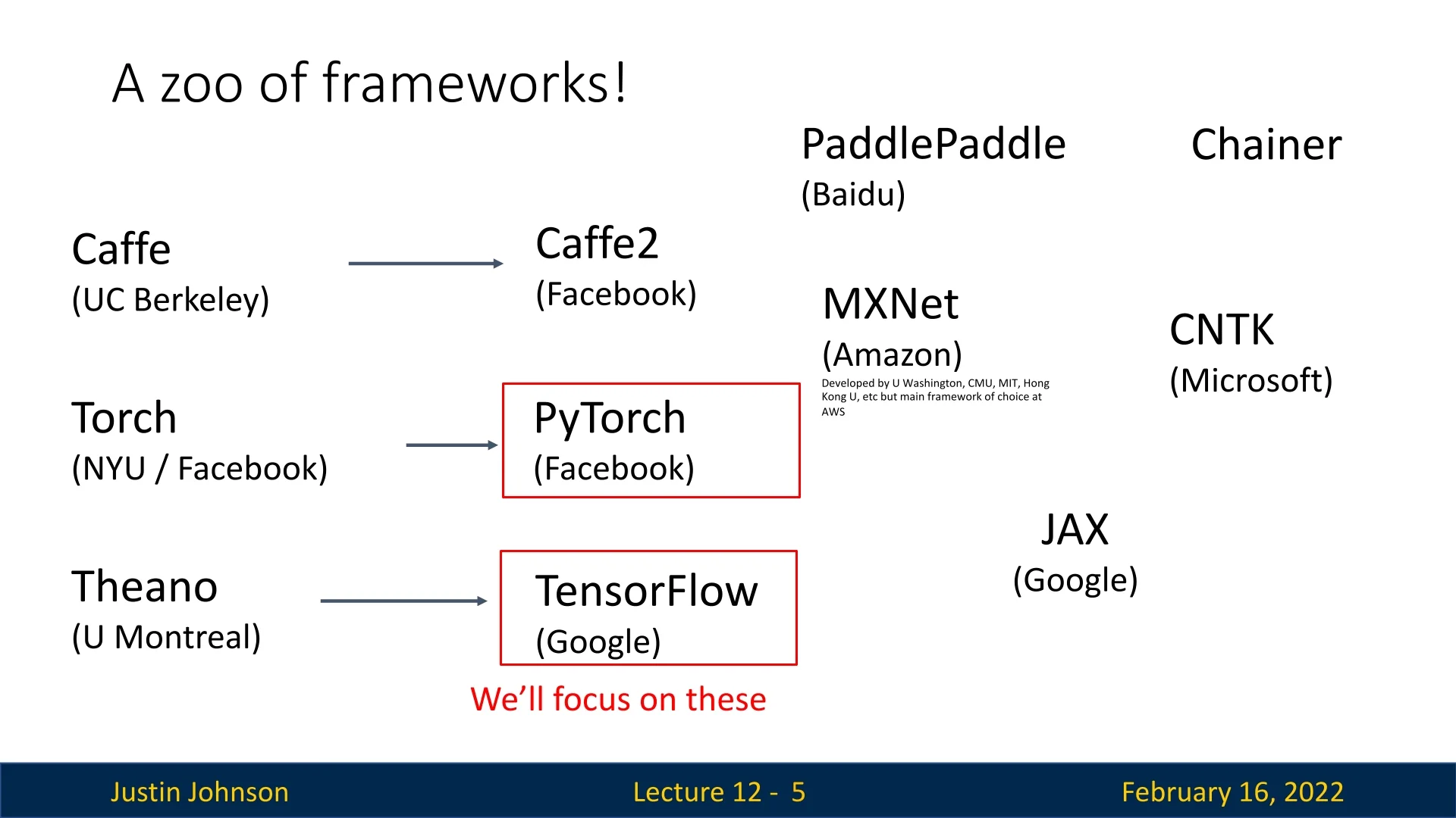
Some notable frameworks include:

• Caffe (UC Berkeley) – One of the earliest frameworks, optimized for speed but limited in flexibility.
• Theano (U. Montreal) – A pioneer in automatic differentiation, but now discontinued.
• TensorFlow (Google) – Popular for production deployments; originally focused on static computation graphs.
• PyTorch (Facebook) – An imperative, Pythonic framework with dynamic computation graphs, widely used in research.
• MXNet (Amazon) – Developed by multiple institutions, designed for distributed deep learning.
• JAX (Google) – A newer framework optimized for high-performance computing and auto-differentiation.

While many frameworks exist, PyTorch and TensorFlow dominate deep learning research and deployment. The following sections explore these frameworks in detail, starting with computational graphs and automatic differentiation.

12.1.1 The Purpose of Deep Learning Frameworks

Deep learning frameworks provide essential tools that simplify the implementation, training, and deployment of neural networks. They abstract away low-level operations, enabling users to focus on model design and experimentation rather than manual gradient computations or hardware-specific optimizations. The three primary goals of deep learning frameworks are:

• Rapid Prototyping: Frameworks allow researchers to quickly experiment with new architectures, optimization techniques, and data pipelines. High-level APIs simplify model definition, while flexible debugging tools enable faster iteration.
• Automatic Differentiation: Modern frameworks automatically compute gradients via backpropagation, eliminating the need for manual derivative calculations. This accelerates research and reduces implementation errors.
• Efficient Execution on Hardware: Frameworks optimize computations for GPUs & TPUs, leveraging parallel processing and efficient memory management to accelerate training and inference.

12.1.2 Recall: Computational Graphs

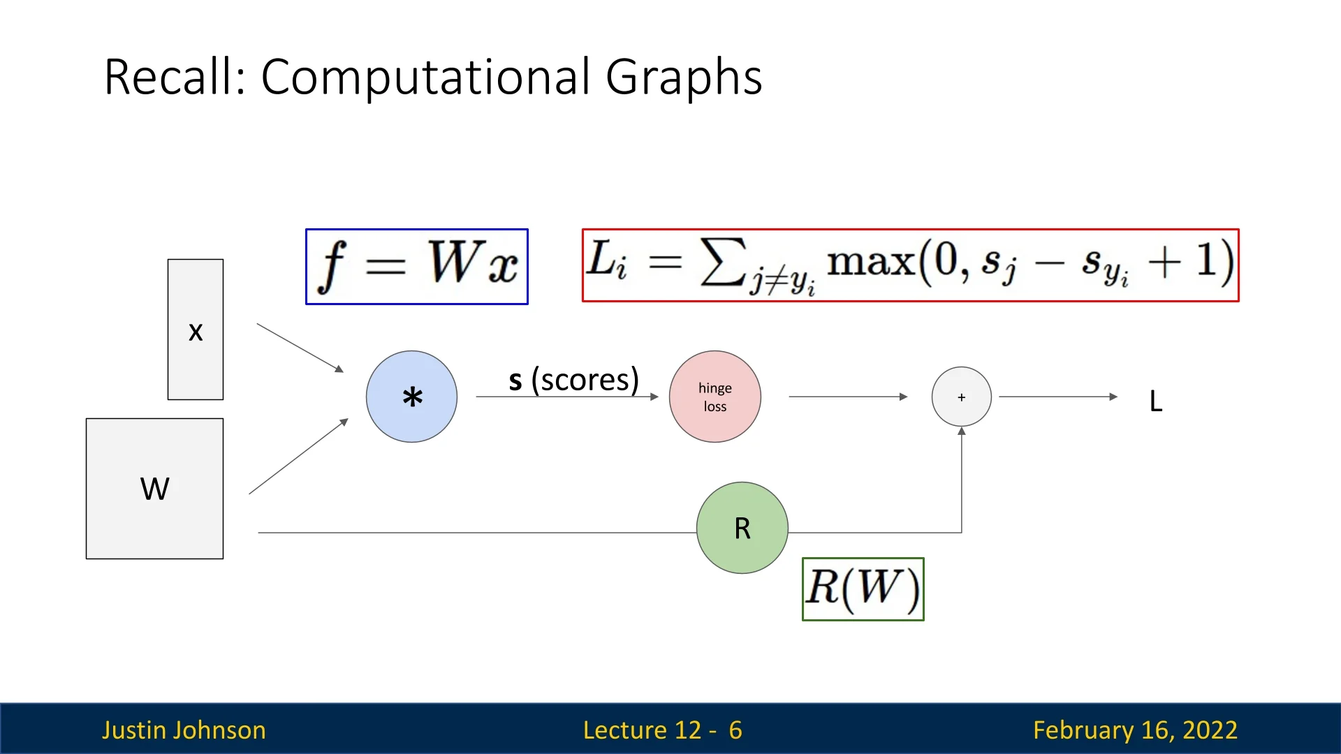
Neural networks are represented as computational graphs. The graphs define the sequence of operations required to compute outputs and gradients during training. A graph consists of:

• Nodes: Represent mathematical operations (e.g., Sigmoid).
• Edges: Represent data flow between operations, forming a directed acyclic graph (DAG).

During training, frameworks use computational graphs to:

1.

Forward Pass: Compute the output by passing data through the graph.

2.

Backward Pass: Compute gradients via backpropagation, traversing the graph in reverse.

3.

Optimization Step: Update parameters using computed gradients.

Understanding computational graphs is crucial, as different frameworks implement them in distinct ways. The next sections explore how PyTorch and TensorFlow utilize these graphs, comparing dynamic vs. static computation strategies.

12.2 PyTorch: Fundamental Concepts

PyTorch is a deep learning framework that provides flexibility, dynamic computation graphs, and efficient execution on both CPUs and GPUs. It introduces key abstractions:

• Tensors: Multi-dimensional arrays similar to NumPy arrays but capable of running on GPUs.
• Modules: Objects representing layers of a neural network, potentially storing learnable parameters.
• Autograd: A system that automatically computes gradients by building computational graphs dynamically.

12.2.1 Tensors and Basic Computation

To illustrate PyTorch’s fundamentals, consider a simple two-layer ReLU network trained using gradient descent on random data.

import torch
device = torch.device(’cpu’)  # Change to ’cuda:0’ to run on GPU
N, D_in, H, D_out = 64, 1000, 100, 10  # Batch size, input, hidden, output dimensions

# Create random tensors for data and weights
x = torch.randn(N, D_in, device=device)
y = torch.randn(N, D_out, device=device)
w1 = torch.randn(D_in, H, device=device)
w2 = torch.randn(H, D_out, device=device)
learning_rate = 1e-6

for t in range(500):
    # Forward pass: compute predictions and loss
    h = x.mm(w1)  # Matrix multiply (fully connected layer)
    h_relu = h.clamp(min=0)  # Apply ReLU non-linearity
    y_pred = h_relu.mm(w2)  # Output prediction
    loss = (y_pred - y).pow(2).sum()  # Compute L2 loss

# Backward pass: manually compute gradients
grad_y_pred = 2.0 * (y_pred - y)
grad_w2 = h_relu.t().mm(grad_y_pred)
grad_h_relu = grad_y_pred.mm(w2.t())
grad_h = grad_h_relu.clone()
grad_h[h < 0] = 0  # Backpropagate ReLU
grad_w1 = x.t().mm(grad_h)

# Gradient descent step on weights
w1 -= learning_rate * grad_w1  # Gradient update
w2 -= learning_rate * grad_w2

PyTorch tensors operate efficiently on GPUs by simply setting:
device = torch.device(’cuda:0’).

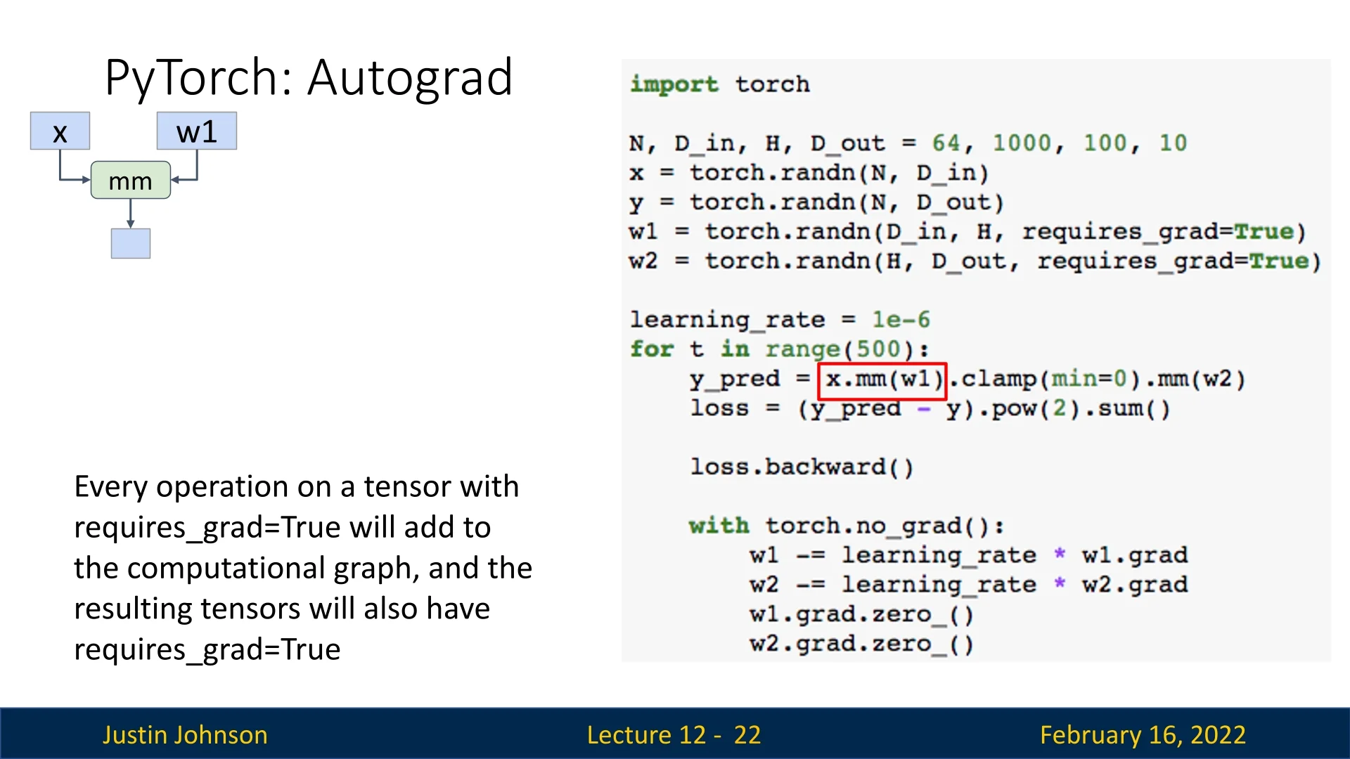
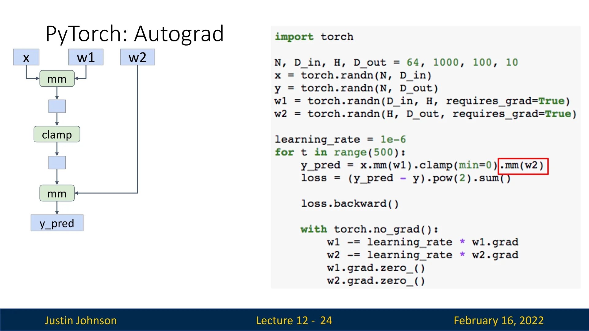
12.2.2 Autograd: Automatic Differentiation

PyTorch’s autograd system automatically builds computational graphs when performing operations on tensors with requires_grad=True. These graphs allow automatic computation of gradients via backpropagation.

x = torch.randn(N, D_in)
y = torch.randn(N, D_out)
w1 = torch.randn(D_in, H, requires_grad=True)
w2 = torch.randn(H, D_out, requires_grad=True)

The forward pass remains unchanged:

h = x.mm(w1)
h_relu = h.clamp(min=0)
y_pred = h_relu.mm(w2)
loss = (y_pred - y).pow(2).sum()  # Compute loss

PyTorch automatically tracks operations and maintains intermediate values, eliminating the need for manual gradient computation. We backpropagate as follows:

loss.backward()  # Computes gradients for w1 and w2

Gradients are accumulated in w1.grad and w2.grad, so we must clear them manually before the next update:

with torch.no_grad():  # Prevents unnecessary graph construction
    w1 -= learning_rate * w1.grad
    w2 -= learning_rate * w2.grad

    w1.grad.zero_()
    w2.grad.zero_()

Forgetting to reset gradients is a common PyTorch bug, as gradients accumulate by default.

12.2.3 Computational Graphs and Modular Computation

PyTorch dynamically constructs computational graphs during forward passes, enabling automatic differentiation and backpropagation. Each tensor operation that involves requires_grad=True contributes to the computational graph.

Building the Computational Graph

The computation graph begins when we perform operations on tensors with requires_grad=True. Consider the following forward pass:

h = x.mm(w1)  # Matrix multiply (fully connected layer)
h_relu = h.clamp(min=0)  # Apply ReLU non-linearity
y_pred = h_relu.mm(w2)  # Output prediction
loss = (y_pred - y).pow(2).sum()  # Compute L2 loss

This sequence of operations results in the following computational graph:

• x.mm(w1) creates a matrix multiplication node with inputs x and w1, producing an output tensor with requires_grad=True.

• .clamp(min=0) applies a ReLU activation, forming another node.

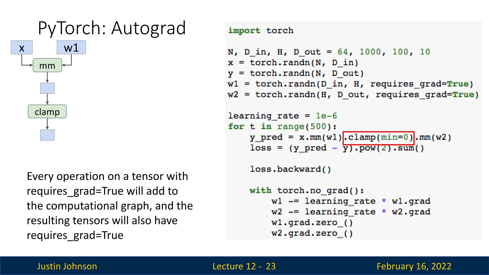
• .mm(w2) applies another matrix multiplication, producing the final prediction.

Loss Computation and Backpropagation

After computing the loss, we backpropagate through the graph to compute gradients:

loss.backward()  # Computes gradients for w1 and w2

During this process:

• (y_pred - y) creates a subtraction node with inputs y_pred and y.
• .pow(2) squares the result, creating a new node.
• .sum() sums the squared differences, outputting a scalar loss.

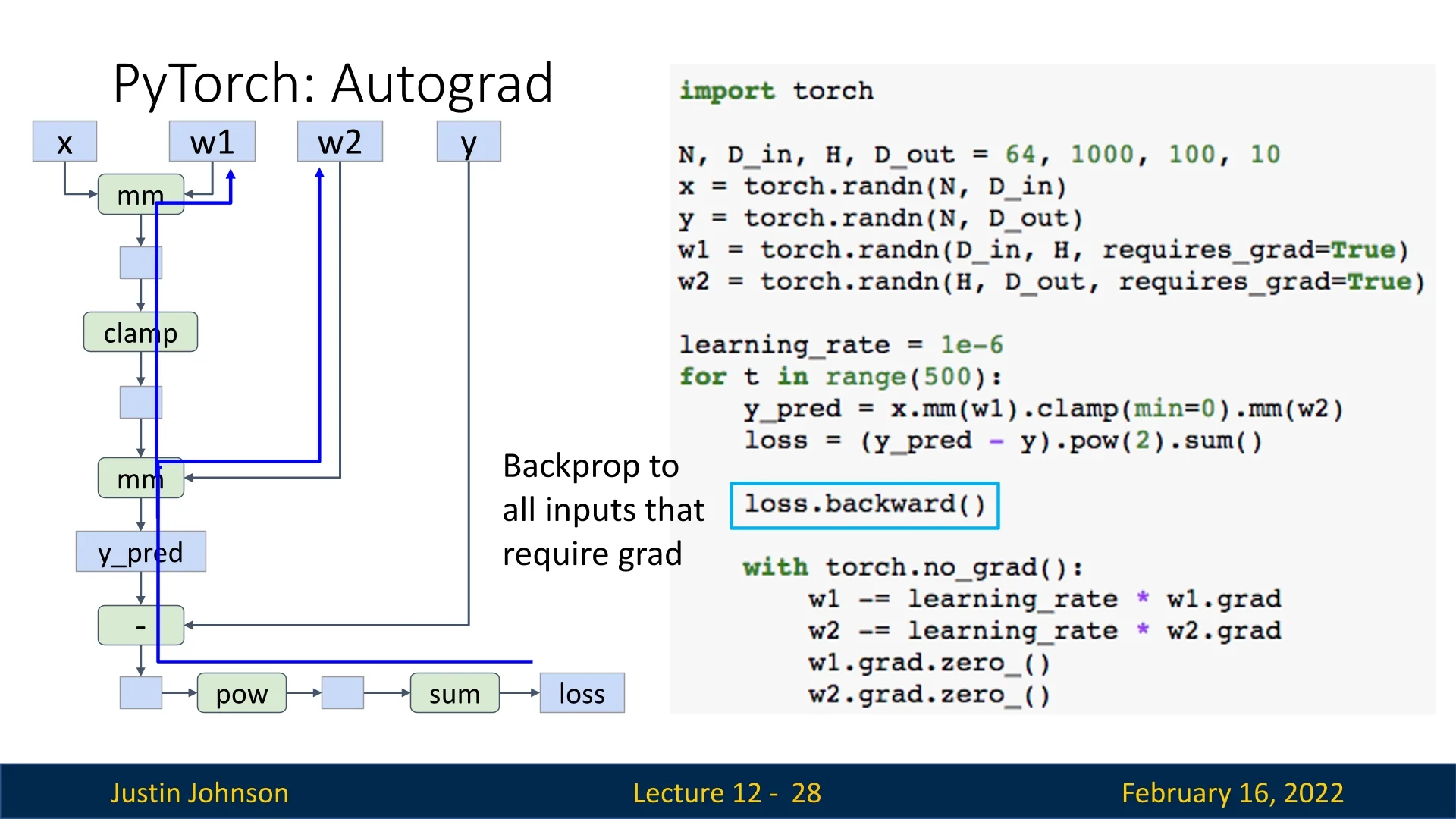
Once gradients are computed, they are stored in w1.grad and w2.grad. However, PyTorch accumulates gradients by default, so they must be cleared before the next update (grad.zero_()):

with torch.no_grad():  # Prevents unnecessary graph construction
    w1 -= learning_rate * w1.grad
    w2 -= learning_rate * w2.grad
    w1.grad.zero_()
    w2.grad.zero_()

Forgetting to reset gradients is a common mistake in PyTorch. Although probably a design flaw in PyTorch, as we usually don’t want to accumulate gradients, we need to be aware of that when we create models.

Extending Computational Graphs with Python Functions

PyTorch’s autograd system allows users to construct computational graphs dynamically using Python functions. When a function is called inside a forward pass, PyTorch records all tensor operations occurring within it.

def custom_relu(x):
    return x.clamp(min=0)  # Element-wise ReLU
    h_relu = custom_relu(h)

Although this function improves code readability, PyTorch still constructs the same computational graph as if we had used .clamp(min=0) directly.

Custom Autograd Functions

PyTorch’s automatic differentiation works by building a computational graph out of primitive operations (e.g., add, mul, exp) and then applying the chain rule. In most cases this is sufficient, but sometimes we want:

• To treat a whole computation as a single semantic unit in the graph (cleaner, fewer nodes, less bookkeeping).
• To override the automatically derived backward with a numerically more stable or more efficient formula.

For this, PyTorch lets us define custom operations by subclassing torch.autograd.Function and explicitly specifying forward and backward.

Motivating Example: Sigmoid A naive Python implementation of the sigmoid is:

def sigmoid(x):
    return 1.0 / (1.0 + torch.exp(-x))

This looks harmless, but it can introduce numerical issues in deep networks:

• For very large negative inputs \(x \ll 0\), we compute torch.exp(-x) = exp(large positive), which overflows to inf in float32. The forward result is still \(1/(1+\infty ) \approx 0\), so we might not notice.
• However, during backward, autograd differentiates through these primitives and uses the same intermediate inf values. Expressions such as \(\frac {\infty }{(1+\infty )^2}\) or \(\infty \cdot 0\) can appear, which numerically become nan, even though the true derivative is \(0\).

Mathematically, the derivative of the sigmoid is \[ \sigma '(x) = \sigma (x)\,(1 - \sigma (x)), \] and this is perfectly stable: once we know \(y = \sigma (x) \in (0,1)\), the product \(y(1-y)\) is always bounded in \([0, 0.25]\) and never overflows. So a more stable strategy is:

1.

Compute \(y = \sigma (x)\) in the forward pass.

2.

Save \(y\).

3.

Compute the gradient in backward using \(y(1-y)\) instead of recomputing exponentials.

This is exactly what a custom autograd function allows us to do.

class Sigmoid(torch.autograd.Function):
    @staticmethod
    def forward(ctx, x):
        # Forward as usual (PyTorch’s built-in sigmoid is already stable;
        # here we reimplement it for illustration).
        y = 1.0 / (1.0 + torch.exp(-x))
        # Save only the stable output y for backward.
        ctx.save_for_backward(y)
        return y

@staticmethod
def backward(ctx, grad_y):
    # Retrieve saved output
    (y,) = ctx.saved_tensors
    # Use the stable formula seen earlier
    grad_x = grad_y * y * (1.0 - y)
    return grad_x


def sigmoid(x):
    return Sigmoid.apply(x)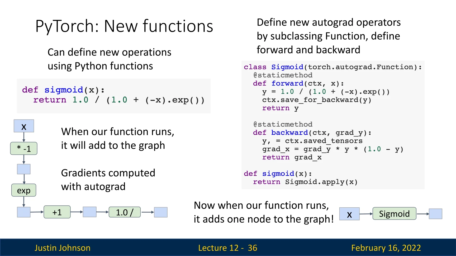

Once defined, we can use the new sigmoid as any other PyTorch operation:

x = torch.randn(10, requires_grad=True)
sigmoid_out = sigmoid(x)
sigmoid_out.sum().backward()

In practice, this level of control is rarely needed for basic operations: PyTorch’s built-in functions (torch.sigmoid, torch.softmax, etc.) are already implemented internally using optimized and stable autograd functions.

Custom Functions become most useful when implementing new layers, composite operations, or specialized losses where we know a better backward formula than the one autograd would derive automatically.

Summary: Backpropagation and Graph Optimization

• Any operation on a tensor with requires_grad=True extends the computational graph.
• PyTorch dynamically records these operations and stores just enough context (saved tensors) to evaluate gradients efficiently via the chain rule.
• Forgetting to reset gradients (e.g., omitting optimizer.zero_grad()) causes gradients to accumulate across iterations, leading to incorrect updates.
• Graph structure can be optimized using custom autograd functions: they fuse multiple primitive ops into a single node, can implement numerically stable backward formulas, and provide more meaningful graph semantics than low-level primitives alone.

A solid understanding of PyTorch’s computational graphs—and how to customize them when necessary—is essential for debugging, improving numerical robustness, and optimizing the performance of deep learning models.

12.2.4 High-Level Abstractions in PyTorch: torch.nn and Optimizers

PyTorch provides a high-level wrapper, torch.nn, which simplifies neural network construction by offering an object-oriented API for defining models. This abstraction allows for more structured and maintainable code, making deep learning models easier to build and extend.

Using torch.nn.Sequential

The torch.nn.Sequential container allows defining models as a sequence of layers. Below, we define a simple two-layer network with ReLU activation:

import torch

N, D_in, H, D_out = 64, 1000, 100, 10
x = torch.randn(N, D_in)
y = torch.randn(N, D_out)

model = torch.nn.Sequential(
    torch.nn.Linear(D_in, H),
    torch.nn.ReLU(),
    torch.nn.Linear(H, D_out)
)

learning_rate = 1e-2
for t in range(500):
    y_pred = model(x)
    loss = torch.nn.functional.mse_loss(y_pred, y)
    loss.backward()

    with torch.no_grad():
        for param in model.parameters():
            param -= learning_rate * param.grad

model.zero_grad()

• The model object is a container holding layers. Each layer manages its own parameters.
• Calling model(x) performs the forward pass.
• The loss is computed using torch.nn.functional.mse_loss().
• Calling loss.backward() computes gradients for all model parameters.
• Parameter updates are performed manually in a loop over model.parameters().
• Calling model.zero_grad() resets gradients for all parameters.

Using Optimizers: Automating Gradient Descent

Instead of manually implementing gradient descent, PyTorch provides optimizer classes that handle parameter updates. Below, we use the Adam optimizer:

import torch

N, D_in, H, D_out = 64, 1000, 100, 10
x = torch.randn(N, D_in)
y = torch.randn(N, D_out)

model = torch.nn.Sequential(
    torch.nn.Linear(D_in, H),
    torch.nn.ReLU(),
    torch.nn.Linear(H, D_out)
)

learning_rate = 1e-4
optimizer = torch.optim.Adam(model.parameters(), lr=learning_rate)

for t in range(500):
    y_pred = model(x)
    loss = torch.nn.functional.mse_loss(y_pred, y)
    loss.backward()

    optimizer.step()
    optimizer.zero_grad()

• The optimizer is instantiated with torch.optim.Adam() and receives model parameters.
• Calling optimizer.step() updates all parameters automatically.
• Calling optimizer.zero_grad() resets gradients before the next step.

This approach is both cleaner and less error-prone than manual updates.

Defining Custom nn.Module Subclasses

For more complex architectures, we can define custom nn.Module subclasses:

import torch


class TwoLayerNet(torch.nn.Module):
    def __init__(self, D_in, H, D_out):
        super(TwoLayerNet, self).__init__()
        self.linear1 = torch.nn.Linear(D_in, H)
        self.linear2 = torch.nn.Linear(H, D_out)

    def forward(self, x):
        h_relu = self.linear1(x).clamp(min=0)
        y_pred = self.linear2(h_relu)
        return y_pred


N, D_in, H, D_out = 64, 1000, 100, 10
x = torch.randn(N, D_in)
y = torch.randn(N, D_out)

model = TwoLayerNet(D_in, H, D_out)
optimizer = torch.optim.SGD(model.parameters(), lr=1e-4)

for t in range(500):
    y_pred = model(x)
    loss = torch.nn.functional.mse_loss(y_pred, y)
    loss.backward()

    optimizer.step()
    optimizer.zero_grad()

• Model Initialization: The __init__ method defines layers as class attributes.
• Forward Pass: The forward() method specifies how inputs are transformed.
• Autograd Integration: PyTorch automatically tracks gradients for model parameters.
• Training Loop: The optimizer updates weights based on computed gradients.

Key Takeaways

• torch.nn.Sequential simplifies defining networks as a stack of layers.
• Optimizers automate gradient descent, making training loops cleaner.
• Custom nn.Module subclasses provide flexibility for complex architectures.
• Autograd handles differentiation automatically, eliminating the need for manual backward computations.

Using torch.nn and optimizers streamlines model development, making PyTorch a powerful and expressive framework for deep learning.

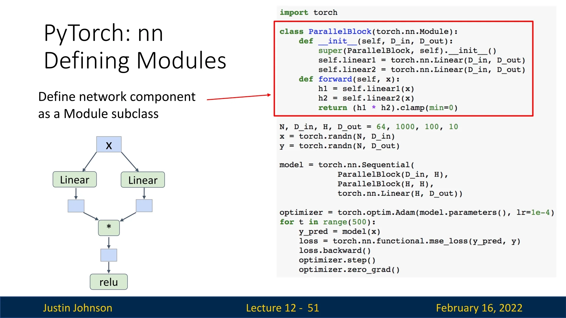
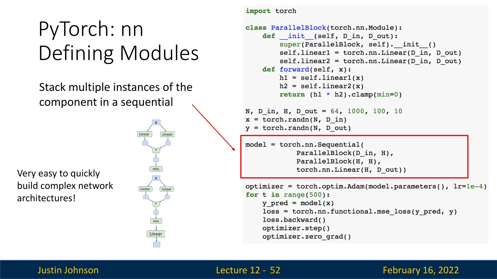
12.2.5 Combining Custom Modules with Sequential Models

A common practice in PyTorch is to combine custom nn.Module subclasses with torch.nn.Sequential containers. This enables modular and scalable architectures while maintaining the expressiveness of object-oriented model design.

Example: Parallel Block

The following example defines a ParallelBlock module that applies two linear transformations to the input independently and then multiplies the results element-wise:

import torch


class ParallelBlock(torch.nn.Module):
    def __init__(self, D_in, D_out):
        super(ParallelBlock, self).__init__()
        self.linear1 = torch.nn.Linear(D_in, D_out)
        self.linear2 = torch.nn.Linear(D_in, D_out)

    def forward(self, x):
        h1 = self.linear1(x)
        h2 = self.linear2(x)
        return (h1 * h2).clamp(min=0)  # Element-wise multiplication followed by ReLU


N, D_in, H, D_out = 64, 1000, 100, 10
x = torch.randn(N, D_in)
y = torch.randn(N, D_out)

model = torch.nn.Sequential(
    ParallelBlock(D_in, H),
    ParallelBlock(H, H),
    torch.nn.Linear(H, D_out)
)

optimizer = torch.optim.Adam(model.parameters(), lr=1e-4)

for t in range(500):
    y_pred = model(x)
    loss = torch.nn.functional.mse_loss(y_pred, y)
    loss.backward()
    optimizer.step()
    optimizer.zero_grad()

• The ParallelBlock applies two separate linear layers to the input.
• The outputs are multiplied element-wise before applying ReLU.
• The Sequential container stacks multiple ParallelBlock instances, followed by a final linear layer.
• Using this approach allows rapid experimentation with modular neural network components.

Although this example is not very smart and not thing we should in practice, it demonstrates well the ability to create building blocks using torch and thus create using this abstraction some complex neural networks with ease.

12.2.6 Efficient Data Loading with torch.utils.data

Training deep neural networks efficiently requires a robust data pipeline. PyTorch provides the torch.utils.data module, which abstracts away data loading, shuffling, batching, and parallelization—ensuring that model computation and data preparation can run concurrently. The two key components are:

• Dataset: Represents a collection of samples. You can use built-in classes like TensorDataset for in-memory tensors or implement a custom Dataset that reads from files or databases.
• DataLoader: Wraps a Dataset to provide mini-batching, shuffling, and multi-process data loading. It also supports pinned memory for faster GPU transfer.

Example: Using DataLoader for Mini-batching

The example below demonstrates how to use DataLoader with synthetic data for mini-batch training.

import torch
    from torch.utils.data import TensorDataset, DataLoader 

    # 1. Create a simple in-memory dataset 
    N, D_in, H, D_out = 64, 1000, 100, 10 
    x = torch.randn(N, D_in) 
    y = torch.randn(N, D_out) 

    dataset = TensorDataset(x, y) 

    # 2. Create a DataLoader with batching and parallel loading 
    loader = DataLoader( 
    dataset, 
    batch_size=8, 
    shuffle=True,      # Shuffle each epoch for stable training 
    num_workers=2,     # Parallel CPU workers for background loading 
    pin_memory=True    # Speeds up host<span class="tctt-1095">→</span>GPU transfers 
    ) 

    model = TwoLayerNet(D_in, H, D_out) 
    optimizer = torch.optim.SGD(model.parameters(), lr=1e-2) 

    # 3. Training loop using the DataLoader 
for epoch in range(20): 
    for x_batch, y_batch in loader: 
        y_pred = model(x_batch) 
        loss = torch.nn.functional.mse_loss(y_pred, y_batch) 

        loss.backward() 
        optimizer.step() 
        optimizer.zero_grad()

This setup automatically handles mini-batch creation, shuffling, and memory prefetching. With num_workers > 0, the CPU preloads data while the GPU trains on the previous batch, preventing GPU idle time—a crucial optimization for large datasets.

Best Practices

• Use shuffle=True to avoid order bias and improve gradient diversity.
• Adjust num_workers to match your CPU cores (typical range: 2–8) for best throughput.
• Set pin_memory=True when training on GPU to accelerate host–device transfers.

Handling Multiple Datasets

In practice, data often comes from multiple sources—different domains, modalities, or tasks. PyTorch offers flexible tools to combine and balance these datasets efficiently.

Concatenating Datasets When datasets share the same structure (e.g., same feature dimensions), use ConcatDataset to merge them into a single unified dataset.

from torch.utils.data import ConcatDataset, DataLoader

dataset_a = TensorDataset(torch.randn(100, 20), torch.randn(100, 1))
dataset_b = TensorDataset(torch.randn(200, 20), torch.randn(200, 1))

combined = ConcatDataset([dataset_a, dataset_b])

loader = DataLoader(
    combined,
    batch_size=16,
    shuffle=True,
    num_workers=4
)

This approach interleaves samples from all datasets proportionally to their sizes. It is ideal for combining related sources (e.g., merging multiple corpora or image datasets).

Weighted Sampling Across Datasets If some datasets are much smaller or more important, you can balance sampling probabilities using WeightedRandomSampler. This ensures underrepresented data appears more frequently in training batches.

from torch.utils.data import WeightedRandomSampler

# Example: emphasize smaller dataset (dataset_a)
weights = [1.0 / len(dataset_a)] * len(dataset_a) + \ 
[1.0 / len(dataset_b)] * len(dataset_b) 

sampler = WeightedRandomSampler(weights, num_samples=len(weights), replacement=True) 

balanced_loader = DataLoader( 
combined, 
batch_size=16, 
sampler=sampler, 
num_workers=4 
)

Weighted sampling is especially useful for:

• Imbalanced datasets. For example, when rare classes need more representation during training.
• Multi-source training. Combining labeled and unlabeled data or datasets from distinct domains.
• Curriculum learning. Gradually increasing sample difficulty or diversity over time.

Streaming or Multi-modal Data For more dynamic or heterogeneous sources (e.g., loading text and image pairs), subclass IterableDataset to yield samples from multiple streams in real time, or define a custom Sampler to coordinate multi-modal alignment.

from torch.utils.data import IterableDataset


class MultiSourceStream(IterableDataset):
    def __iter__(self):
        for x_img, x_txt in zip(image_stream(), text_stream()):
            yield preprocess(x_img, x_txt)

This design is common in large-scale vision–language or multi-task training pipelines, where data arrives asynchronously or from external APIs.

Summary DataLoader and its related utilities form the backbone of efficient training in PyTorch. They decouple data I/O from model computation, provide clean abstractions for multi-source or imbalanced data, and make large-scale experiments reproducible and scalable across CPUs and GPUs.

12.2.7 Using Pretrained Models with TorchVision

PyTorch provides access to many pretrained models through the torchvision package, making it easy to leverage existing architectures for various vision tasks.

Using pretrained models is as simple as:

import torchvision.models as models

alexnet = models.alexnet(pretrained=True)
vgg16 = models.vgg16(pretrained=True)
resnet101 = models.resnet101(pretrained=True)

• These models come with pretrained weights on ImageNet, making them suitable for transfer learning.
• Fine-tuning pretrained models often leads to faster convergence and better performance on new tasks.
• torchvision.models provides a wide variety of architectures beyond AlexNet, VGG, and ResNet.

Key Takeaways

• Custom modules and torch.nn.Sequential can be combined to quickly build complex models while maintaining modularity.
• Data loading utilities such as torch.utils.data.DataLoader facilitate efficient mini-batching and dataset management.
• TorchVision provides pretrained models, making it easy to leverage state-of-the-art architectures for various vision tasks.

12.3 Dynamic vs. Static Computational Graphs in PyTorch

A fundamental design choice in PyTorch is its use of dynamic computational graphs. Unlike static graphs, which are constructed once and reused, PyTorch builds a fresh computational graph for each forward pass. Once loss.backward() is called, the graph is discarded, and a new one is constructed in the next iteration.

While dynamically building graphs in every iteration may seem inefficient, this approach provides a crucial advantage: the ability to use standard Python control flow during model execution. This enables complex architectures that modify their behavior on-the-fly based on intermediate results.

Example: Dynamic Graph Construction

Consider a model where the choice of weight matrix for backpropagation depends on the previous loss value. This scenario, though impractical, demonstrates PyTorch’s ability to create different computational graphs in each iteration.

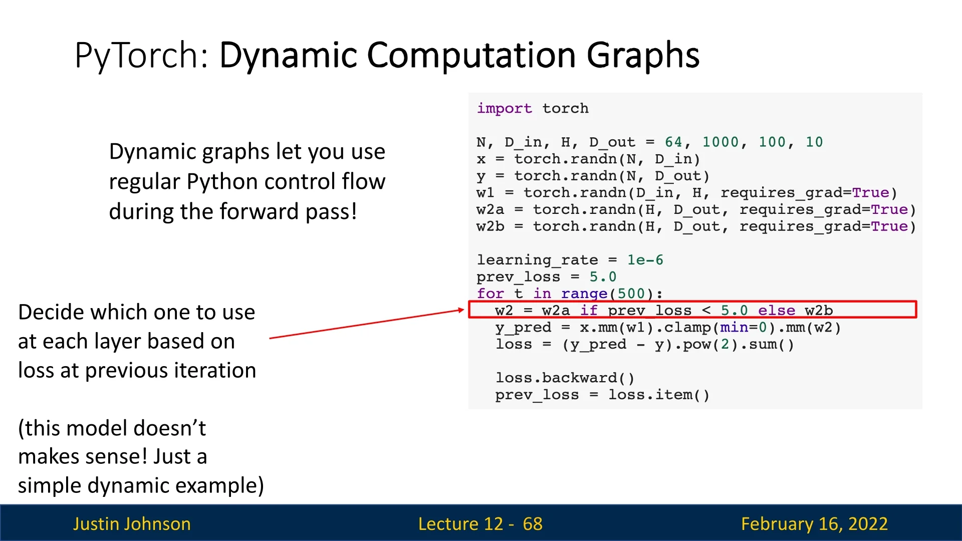
In dynamic graphs, every forward pass constructs a unique computation graph, allowing for models with varying execution paths across different iterations.

12.3.1 Static Graphs and Just-in-Time (JIT) Compilation

In contrast, static computational graphs follow a two-step process:

1.

Graph Construction: Define the computational graph once, allowing the framework to optimize it before execution.

2.

Graph Execution: The same pre-optimized graph is reused for all forward passes.

While PyTorch natively operates with dynamic graphs, it also supports static graphs through TorchScript using Just-in-Time (JIT) compilation. This allows PyTorch to analyze the model’s source code, compile it into an optimized static graph, and reuse it for improved efficiency.

12.3.2 Using JIT to Create Static Graphs

To convert a function into a static computational graph, PyTorch provides torch.jit.script():

import torch


def model(x):
    return x * torch.sin(x)


scripted_model = torch.jit.script(model)  # Convert to static graph

Alternatively, PyTorch allows automatic graph compilation using the @torch.jit.script annotation:

import torch


@torch.jit.script
def model(x):
    return x * torch.sin(x)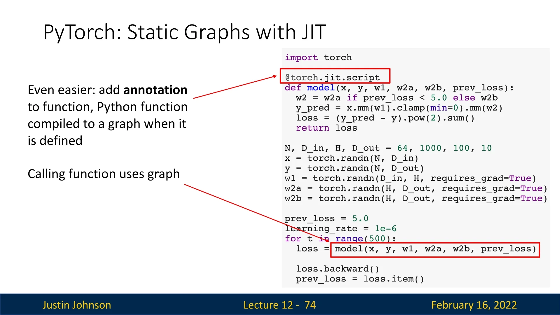

12.3.3 Handling Conditionals in Static Graphs

Static graphs struggle with conditionals because they are typically fixed at compile time. However, PyTorch’s JIT can represent conditionals as graph nodes, enabling runtime flexibility.

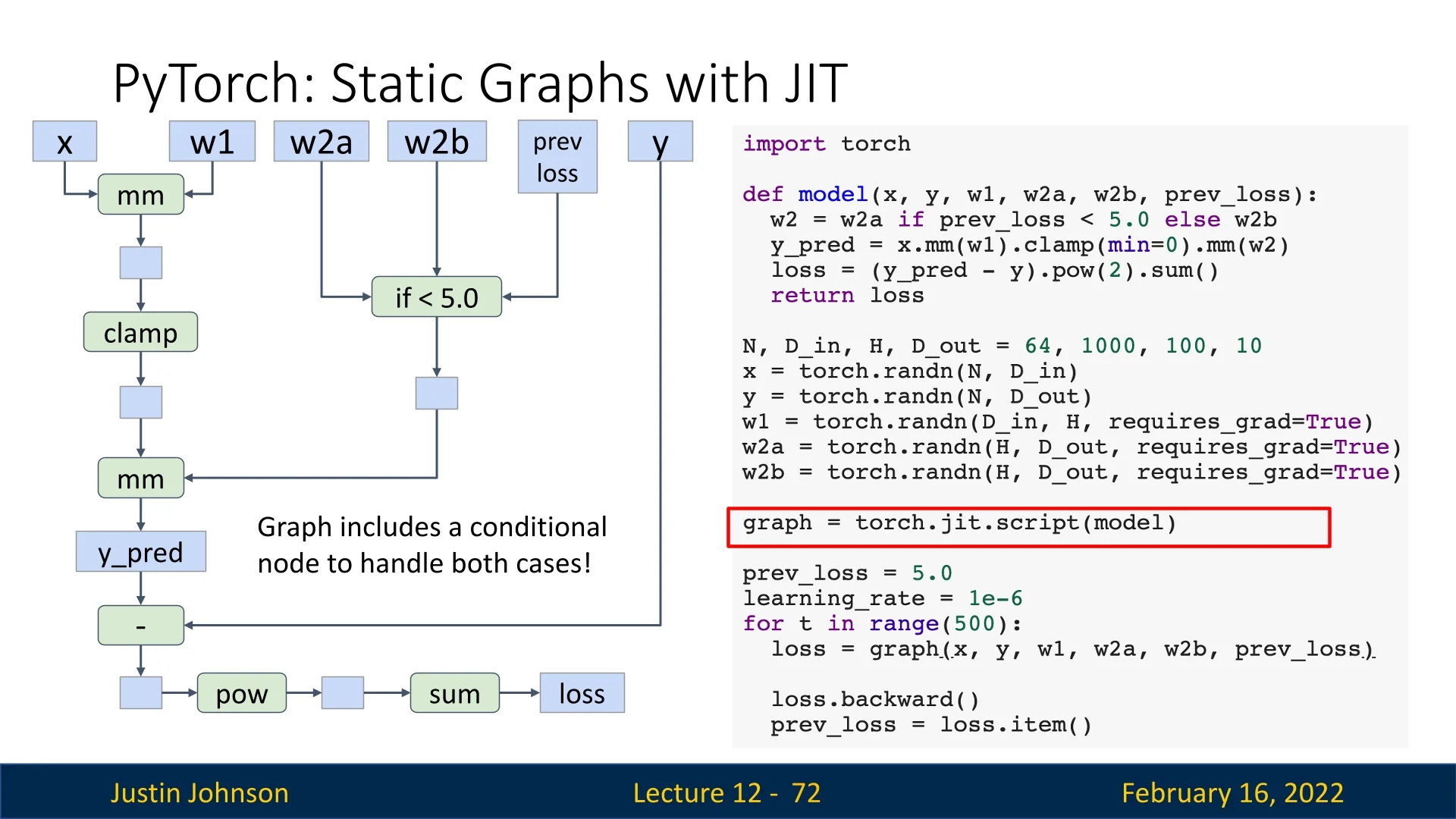
This allows some degree of flexibility while retaining the benefits of graph optimization.

12.3.4 Optimizing Computation Graphs with JIT

One advantage of static graphs is that they enable graph-level optimizations. PyTorch JIT can automatically fuse operations such as convolution and activation layers into a single efficient operation.

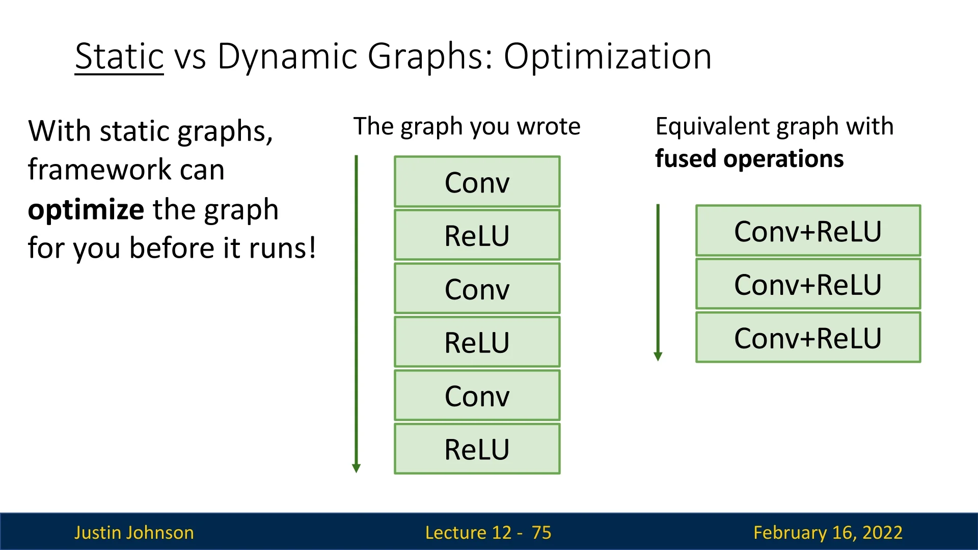
This optimization is performed once, eliminating the need to optimize in every iteration.

12.3.5 Benefits and Limitations of Static Graphs

Advantages of Static Graphs:

• Graph Optimization: The framework optimizes computation before execution, improving speed.
• Operation Fusion: Frequently used layers (e.g., Conv + ReLU) are merged into a single operation.
• Serialization: Models can be saved to disk and loaded in non-Python environments (e.g., C++).

Challenges of Static Graphs:

• Difficult Debugging: Debugging static graphs can be challenging due to indirection between graph construction and execution.
• Less Flexibility: Unlike dynamic graphs, static graphs struggle with models that modify their execution path.
• Rebuilding Required: Any model change requires reconstructing the entire graph.

12.3.6 When Are Dynamic Graphs Necessary?

Certain architectures require dynamic graphs due to their execution dependencies on input data:

• Recurrent Neural Networks (RNNs): The number of computation steps depends on input sequence length.
• Recursive Networks: Hierarchical models, such as parse trees in NLP, require dynamic execution paths.
• Modular Networks: Some architectures dynamically select which sub-network to execute.

A well-known example is the model in [270], where part of the network predicts which module should execute next.

12.4 TensorFlow: Dynamic and Static Computational Graphs

TensorFlow originally adopted static computational graphs by default (TensorFlow 1.0), requiring users to explicitly define a computation graph before running it. However, in TensorFlow 2.0, the framework transitioned to dynamic graphs by default, making the API more similar to PyTorch. This shift caused a significant divide in the TensorFlow ecosystem, as older static-graph code intertwined with newer dynamic-graph code, creating confusion and bugs.

12.4.1 Defining Computational Graphs in TensorFlow 2.0

In PyTorch, the computational graph is built implicitly: any operation performed on a tensor with requires_grad=True is automatically tracked. TensorFlow 2.0 (TF2), by contrast, introduced eager execution as the default mode—operations execute immediately like standard Python code, producing concrete values rather than symbolic graph nodes. This makes TF2 intuitive and debuggable but requires an explicit mechanism for recording operations when gradients are needed. That mechanism is the tf.GradientTape.

Understanding tf.GradientTape

The GradientTape is TensorFlow’s dynamic autodiff engine, analogous to PyTorch’s implicit autograd. It acts like a “recorder”: while active, it logs all operations on watched tensors (typically all tf.Variable objects) and can later “play back” those operations to compute gradients.

• Entering a with tf.GradientTape() as tape: block begins recording.
• Any operation involving watched variables is logged on the tape.
• Exiting the block stops recording.
• Calling tape.gradient(loss, [vars]) replays the tape backward to compute exact gradients via the chain rule.

This explicit opt-in design prevents unnecessary gradient tracking (e.g., during inference) and gives developers fine-grained control over which computations are differentiable.

import tensorflow as tf

# Setup data and parameters
N, Din, H, Dout = 16, 1000, 100, 10
x = tf.random.normal((N, Din))
y = tf.random.normal((N, Dout))
w1 = tf.Variable(tf.random.normal((Din, H)))
w2 = tf.Variable(tf.random.normal((H, Dout)))

learning_rate = 1e-6

for t in range(1000):
    # Begin recording operations on the tape
    with tf.GradientTape() as tape:
        h = tf.maximum(tf.matmul(x, w1), 0)  # ReLU
        y_pred = tf.matmul(h, w2)
        diff = y_pred - y
        loss = tf.reduce_mean(tf.reduce_sum(diff ** 2, axis=1))

    # Compute gradients of loss w.r.t parameters
    grad_w1, grad_w2 = tape.gradient(loss, [w1, w2])

    # Parameter updates (in-place, safe for tf.Variables)
    w1.assign_sub(learning_rate * grad_w1)
    w2.assign_sub(learning_rate * grad_w2)

This process mirrors PyTorch’s autograd but with more explicit control: GradientTape defines the graph’s lifetime (inside the with block), rather than relying on implicit global tracking. The resulting computation graph is ephemeral—destroyed after gradient computation unless the tape is declared as persistent=True (allowing multiple gradient calls).

Key differences from PyTorch

• PyTorch automatically tracks gradients for all tensors with requires_grad=True. TensorFlow records only within the GradientTape context.
• TensorFlow’s graph is discarded after use unless marked persistent.
• GradientTape offers fine-grained control: you can record subsets of operations or specific variables only.

12.4.2 Static Graphs with @tf.function

While TF2 defaults to eager (imperative) execution for flexibility, static computation graphs are still essential for deployment and optimization. To combine both worlds, TensorFlow introduces the @tf.function decorator, which traces Python functions into optimized static graphs—comparable to torch.jit.script() in PyTorch.

Motivation Eager execution simplifies experimentation but adds Python overhead per operation. Static graphs, on the other hand, allow TensorFlow to perform ahead-of-time optimizations: operation fusion (e.g., combining matmul + bias_add), kernel selection, memory reuse, and XLA compilation. Using @tf.function, developers write natural Python code while TensorFlow transparently traces and compiles it.

@tf.function  # Compiles to a static graph on first call
def training_step(x, y, w1, w2, lr):
    with tf.GradientTape() as tape:
        h = tf.maximum(tf.matmul(x, w1), 0)
        y_pred = tf.matmul(h, w2)
        loss = tf.reduce_mean(tf.reduce_sum((y_pred - y) ** 2, axis=1))

    grad_w1, grad_w2 = tape.gradient(loss, [w1, w2])
    w1.assign_sub(lr * grad_w1)
    w2.assign_sub(lr * grad_w2)
    return loss


# Regular Python loop, but graph executes under the hood
for t in range(1000):
    current_loss = training_step(x, y, w1, w2, learning_rate)

Here, @tf.function traces the computation during its first execution, then caches the resulting static graph for reuse—removing Python overhead and enabling runtime optimizations. This achieves up to 2–10\(\times \) speedups for heavy workloads while preserving eager-like syntax.

Summary of Modes

• Eager mode. Operations run immediately, ideal for debugging and experimentation.
• GradientTape. Dynamically records operations for automatic differentiation, similar to PyTorch’s autograd.
• @tf.function. Converts eager code into a reusable static graph, fusing and optimizing operations for deployment.

Together, these tools give TensorFlow 2.0 both the interactivity of PyTorch and the performance advantages of static compilation—bridging the flexibility–efficiency trade-off that defined earlier deep learning frameworks.

12.5 Keras: High-Level API for TensorFlow

Keras provides a high-level API for building deep learning models, simplifying working with models.

import tensorflow as tf
from tensorflow.keras.models import Sequential
from tensorflow.keras.layers import InputLayer, Dense

N, Din, H, Dout = 16, 1000, 100, 10

model = Sequential([
    InputLayer(input_shape=(Din,)),
    Dense(units=H, activation=’relu’),
    Dense(units=Dout)
])

loss_fn = tf.keras.losses.MeanSquaredError()
opt = tf.keras.optimizers.SGD(learning_rate=1e-6)

x = tf.random.normal((N, Din))
y = tf.random.normal((N, Dout))

for t in range(1000):
    with tf.GradientTape() as tape:
        y_pred = model(x)
        loss = loss_fn(y_pred, y)
    grads = tape.gradient(loss, model.trainable_variables)
    opt.apply_gradients(zip(grads, model.trainable_variables))

Keras simplifies training by providing:

• Predefined layers: Easily stack layers with Sequential().
• Common loss functions and optimizers: Use built-in losses and optimizers like Adam.
• Automatic gradient handling: opt.apply_gradients() simplifies parameter updates.

We can further simplify the training loop using opt.minimize() by defining a step function:

def step():
    y_pred = model(x)
    loss = loss_fn(y_pred, y)
    return loss


for t in range(1000):
    opt.minimize(step, model.trainable_variables)

12.6 TensorBoard: Visualizing Training Metrics

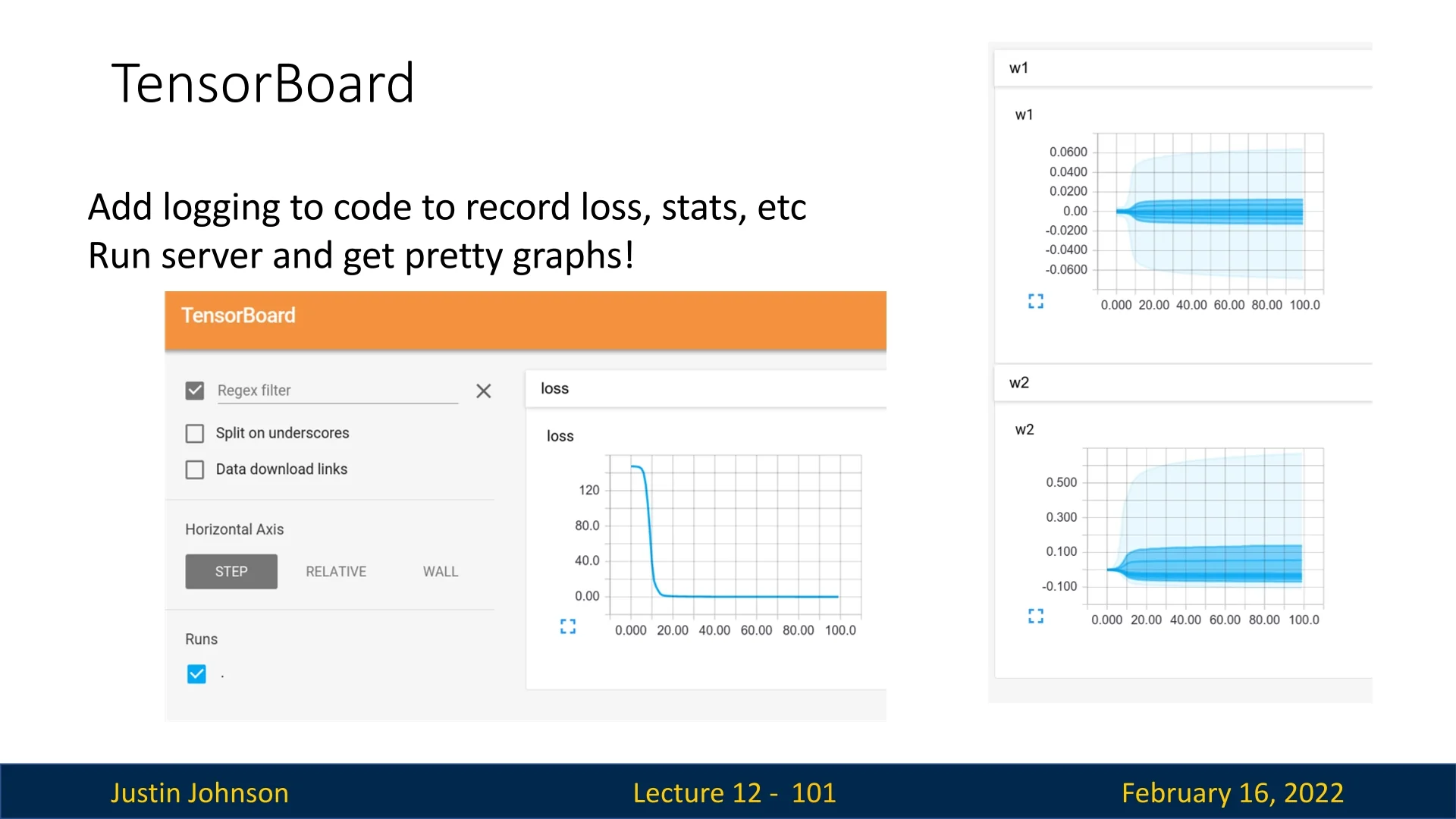
TensorBoard is a visualization tool that helps monitor deep learning experiments. It allows users to track:

• Loss curves and accuracy during training.
• Weight distributions and parameter updates.
• Computational graphs of the model.

While originally designed for TensorFlow, TensorBoard now support PyTorch via the
torch.utils.tensorboard API. However, modern alternatives such as Weights and Biases (wandb) and MLFlow provide additional functionality, making them popular choices for tracking experiments.

12.7 Comparison: PyTorch vs. TensorFlow

• PyTorch:

  • Imperative API that is easy to debug.
  • Dynamic computation graphs enable flexibility.
  • torch.jit.script() allows for static graph compilation.
  • Harder to optimize for TPUs.
  • Deployment on mobile is less streamlined.

• TensorFlow 1.0:

  • Static graphs by default.
  • Faster execution but difficult debugging.
  • API inconsistencies made it less user-friendly.

• TensorFlow 2.0:

  • Defaulted to dynamic graphs, similar to PyTorch.
  • Standardized Keras API for ease of use.
  • Still retains static graph capability with tf.function.

Conclusion Both PyTorch and TensorFlow 2.0 now support both dynamic and static graphs, offering flexibility for different use cases. PyTorch remains the preferred choice for research due to its intuitive imperative style, while TensorFlow is still widely used in production, particularly in environments requiring static graph optimization.