Lecture 2: Image Classification

2.1 Introduction to Image Classification

Image classification is one of the most fundamental tasks in computer vision and serves as the cornerstone for a wide range of applications in artificial intelligence. The objective of image classification is straightforward: given an input image, the algorithm must assign a category label from a predefined set of classes. For instance, an algorithm might label an image as one of several categories, such as ”cat,” ”dog,” or ”car”.

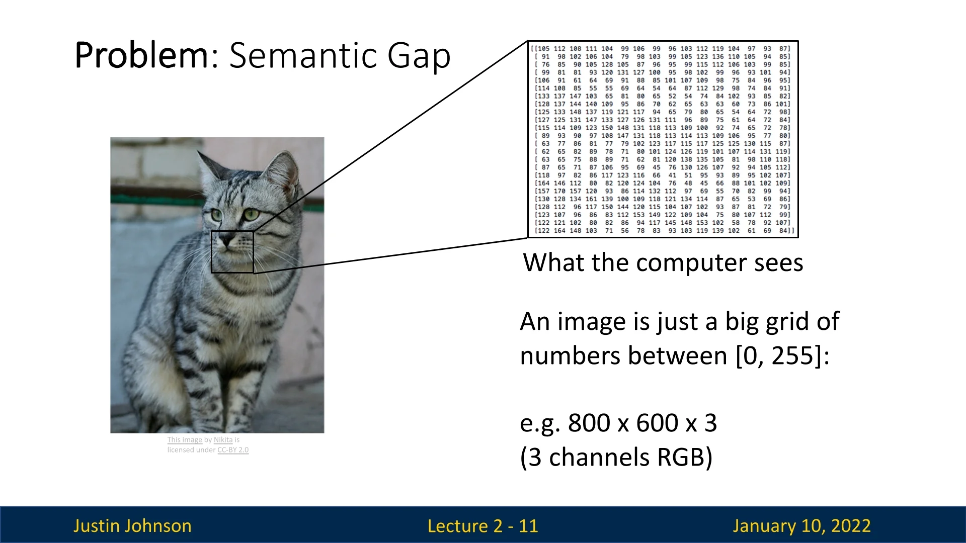
Despite its simplicity in concept, image classification presents a host of challenges when applied to real-world scenarios. Humans effortlessly recognize objects in images due to our ability to intuitively interpret visual information. However, computers face significant hurdles due to the semantic gap, which refers to the difference between the raw pixel values of an image and the high-level semantic information we perceive.

When processing an image, a computer sees only a grid of numbers representing pixel intensities. Even minor changes, such as variations in viewpoint, lighting, or background, can drastically alter these pixel values, making it difficult to map them to a consistent semantic label. Moreover, intra-class variations, such as differences in appearance among individual objects within the same category, add another layer of complexity.

To address these challenges, image classification has evolved from early heuristic-based methods to modern data-driven approaches that leverage machine learning and deep learning. By analyzing large datasets of labeled images, these algorithms learn patterns and statistical dependencies that enable them to generalize across diverse examples.

This chapter begins by exploring the foundational concepts of image classification, including its historical background and early techniques. It then delves into common datasets used for classification, providing insights into their importance and structure. Building on this foundation, we introduce the nearest neighbor algorithm as our first learning-based method, followed by a discussion on hyperparameter tuning, data hygiene, and cross-validation. Finally, the chapter highlights the pivotal role of image classification in powering more advanced computer vision tasks, such as object detection and image captioning, and examines the transition from raw pixel-based methods to feature-based approaches driven by deep learning.

By the end of this chapter, readers will gain a solid understanding of the principles and challenges of image classification and will be equipped with the knowledge to implement their first machine learning algorithm for visual recognition.

2.2 Image Classification Challenges

Image classification is a fundamental yet challenging task in computer vision. It requires algorithms to bridge the ”semantic gap”—the disparity between human perception and raw pixel data processed by machines. This gap arises because machines interpret images as tensors (multidimensional arrays, or a generalization in n dimensions of matrices) of pixel values, devoid of inherent semantic meaning. This section explores the critical challenges in image classification, highlighting the complexities of achieving robust and accurate recognition.

2.2.1 The Semantic Gap

Humans perceive images intuitively, instantly recognizing objects and their context. Machines, however, see images as grids of numbers—pixel values in a tensor representation. For example, an image might be represented as a \(H \times W \times C\) tensor, where \(H\) and \(W\) denote the height and width of the image, and \(C\) represents color channels. These raw values lack semantic information, making it challenging for algorithms to deduce meaningful patterns.

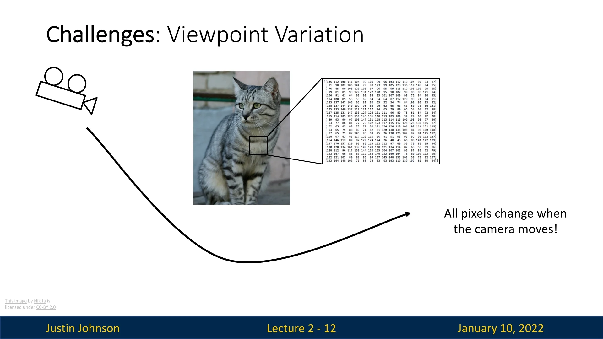
Figure 2.1: Images are represented as grids of pixel values, lacking inherent semantic meaning.

2.2.2 Robustness to Camera Movement

Images captured from different camera angles or positions can vary significantly in their pixel values, even when depicting the same scene. For example, photographing a cat from different angles produces vastly different pixel grids, despite representing the same object.

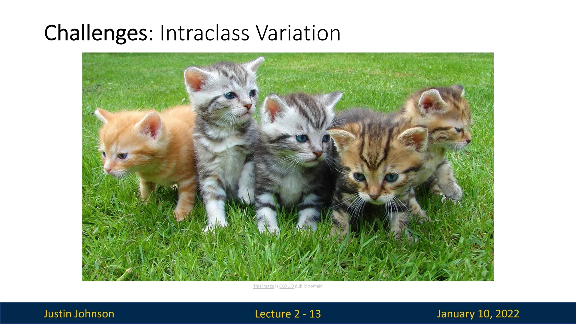
Figure 2.2: Changes in camera position or angle result in varying pixel grids, complicating classification.

2.2.3 Intra-Class Variation

Objects within the same category can exhibit substantial visual differences. For example, cats of different breeds or fur colors might look entirely distinct in terms of pixel patterns.

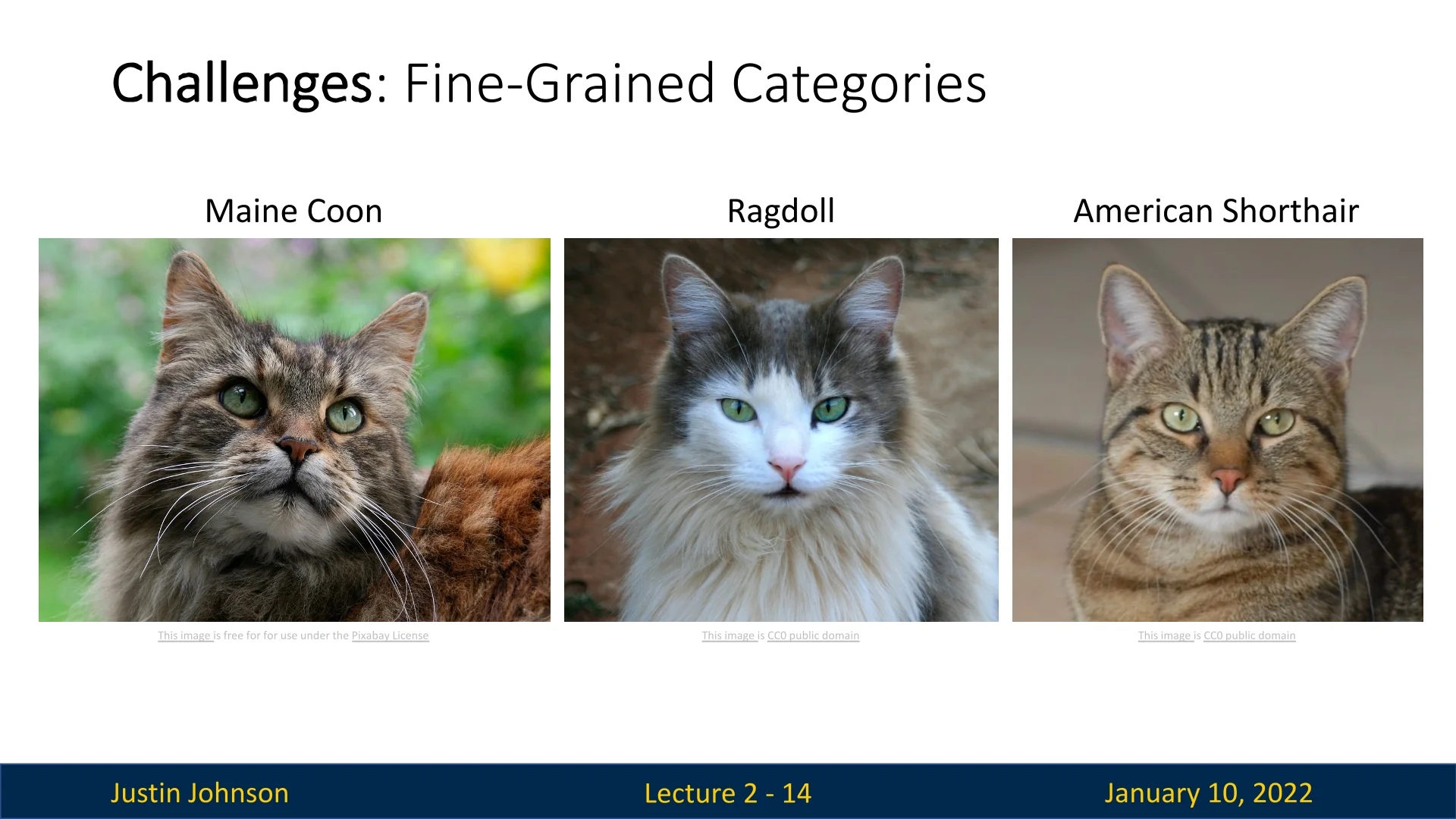
Figure 2.3: Cats of different breeds show significant visual differences, a phenomenon known as intra-class variation.

2.2.4 Fine-Grained Classification

Distinguishing between visually similar categories, such as specific breeds of cats, requires a more granular understanding of features. Fine-grained classification demands algorithms that can differentiate subtle variations within a category, such as fur patterns or ear shapes.

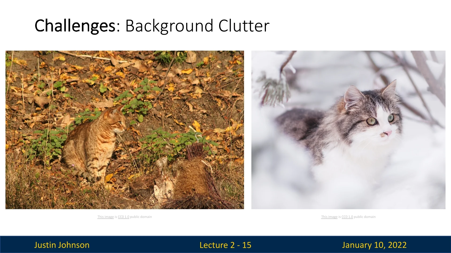
Figure 2.4: Fine-grained classification requires distinguishing subtle differences within visually similar categories.

2.2.5 Background Clutter

Objects in images often blend into complex or cluttered backgrounds, making it challenging to isolate the target object. For instance, a cat sitting amidst foliage may be difficult to distinguish due to natural camouflage or similar textures.

Figure 2.5: Background clutter can obscure target objects, complicating image classification.

2.2.6 Illumination Changes

Lighting conditions significantly impact the appearance of objects in images. A cat photographed in daylight might look very different when captured under dim lighting, even though its semantic identity remains unchanged.

Figure 2.6: Variations in illumination conditions affect object appearance, requiring robust algorithms.

2.2.7 Deformation and Object Scale

Objects are not rigid entities; they deform and appear at varying scales within images. For example, a cat lying stretched out versus curled up occupies different shapes and scales in an image.

Figure 2.7: Objects can deform and appear at varying scales, posing challenges for classification.

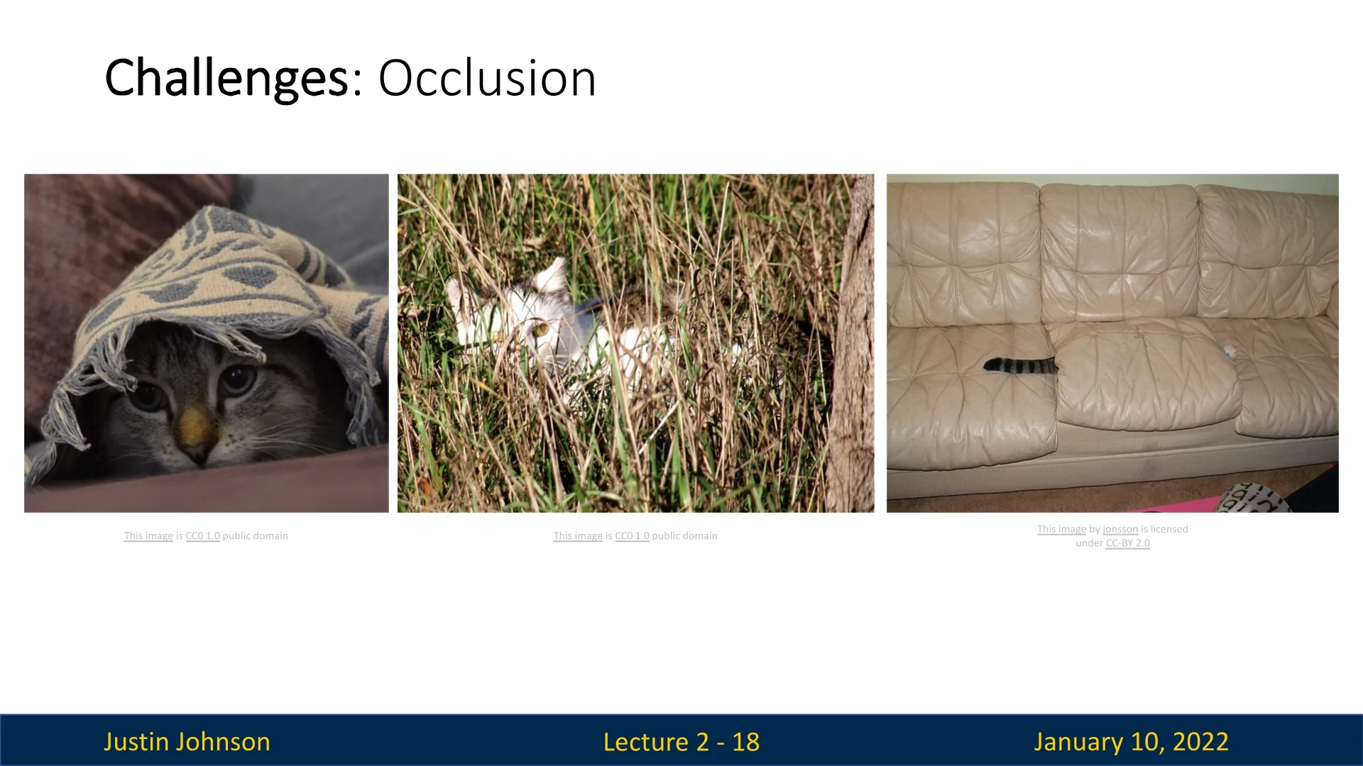
2.2.8 Occlusions

Partial visibility of objects adds another layer of complexity to image classification. For instance, a cat partially hidden under a pillow, with only its tail visible, might be easily recognized by humans based on contextual reasoning. However, such occlusions often hinder algorithmic performance, as they obscure critical features necessary for classification.

Figure 2.8: Occlusions, such as partial visibility of objects, obscure critical features and hinder classification.

2.2.9 Summary of Challenges

Image classification presents a range of challenges rooted in the complexities of visual data and the semantic gap between raw pixel values and meaningful categories. Developing effective algorithms requires bridging this gap while ensuring robustness to variations in viewpoint, illumination, occlusion, deformation, and other real-world conditions.

Traditional approaches to image classification, such as edge detection and corner detection combined with feature descriptors and matching, offered foundational insights into the problem. However, these classical methods often struggled to adapt to the diversity and unpredictability of real-world scenarios, limiting their effectiveness in practical applications.

The emergence of learning-based methods, particularly deep learning, has transformed the landscape by providing more robust and scalable solutions. These methods leverage techniques such as data augmentation and feature extraction to learn hierarchical representations directly from raw data. This ability to adapt and generalize across varying conditions has propelled significant advancements in classification performance, making these approaches the dominant paradigm in the field.

In the following sections, we will delve into these challenges and explore how learning-based methodologies address them.

2.3 Image Classification as a Building Block for Other Tasks

Image classification serves as a foundational task in computer vision, enabling advancements in a variety of related applications. Its ability to assign meaningful labels to visual data allows more complex tasks to be framed as extensions of classification. In this section, we explore how image classification supports tasks such as object detection, image captioning, and decision-making in board games.

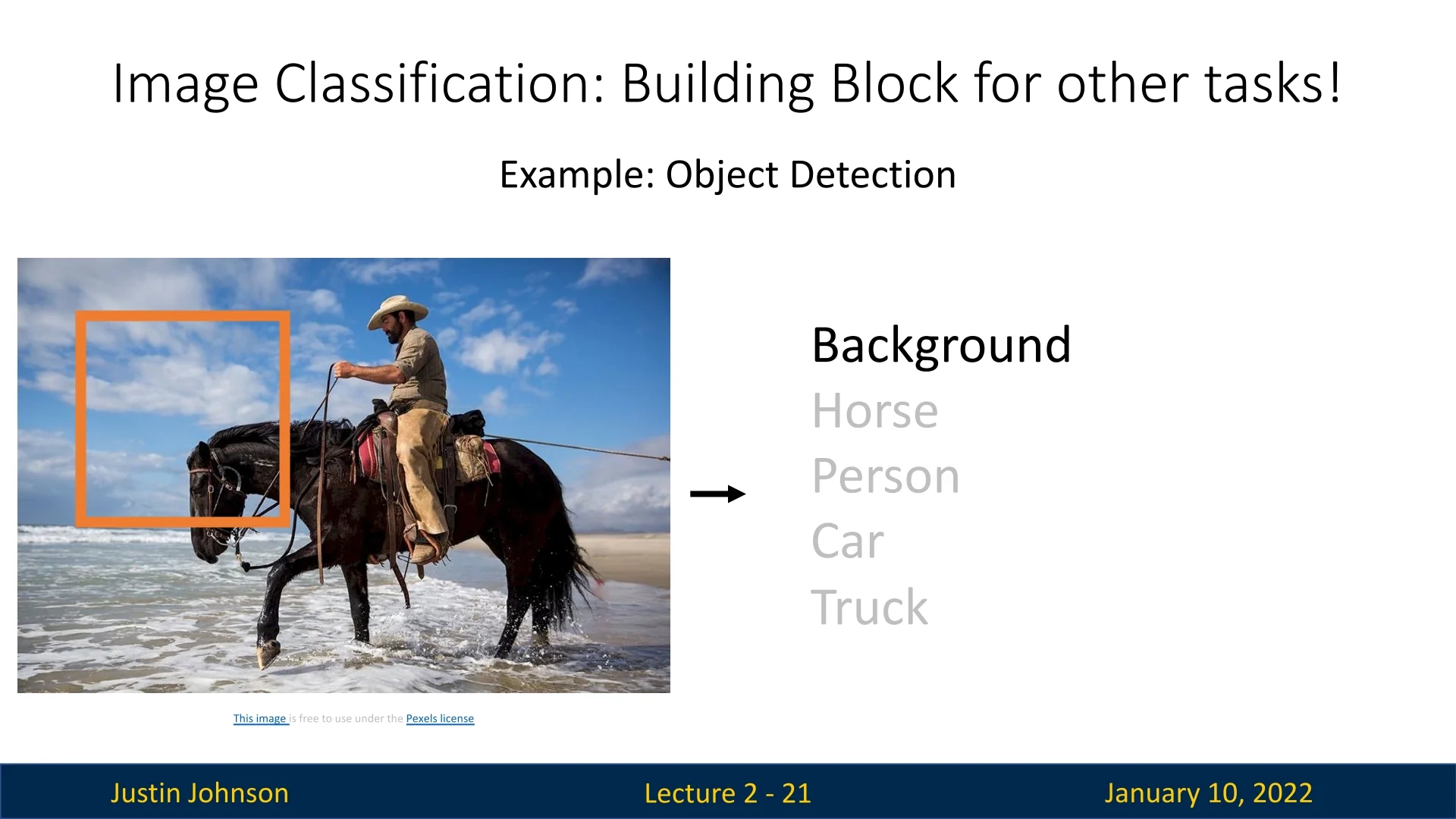
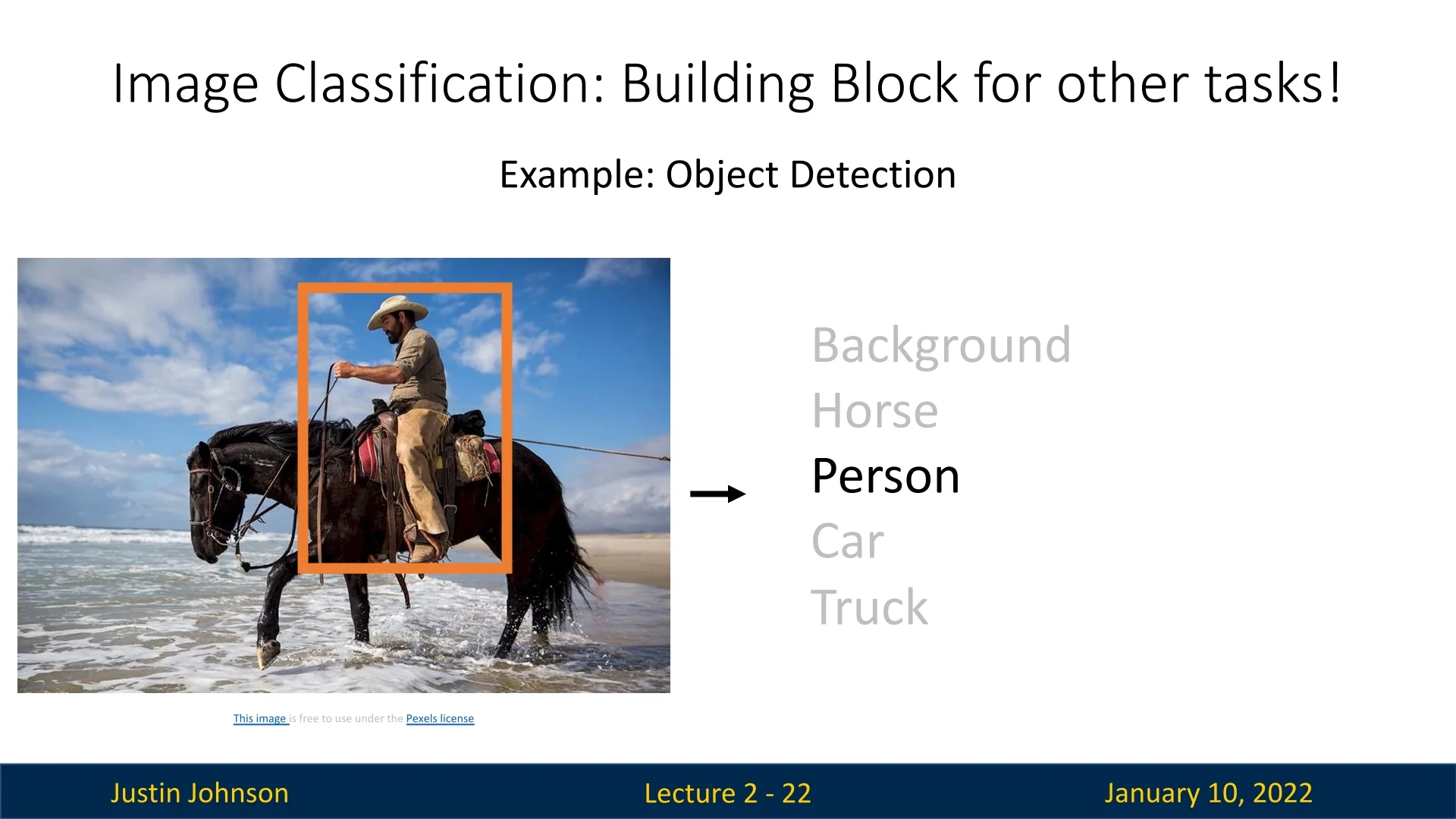
2.3.1 Object Detection

Object detection extends image classification by identifying not only the types of objects present in an image but also their locations. A robust image classifier can be utilized as a core component of an object detection pipeline by classifying regions within an image.

One approach is to use a sliding window technique, where the image is divided into overlapping subregions. Each subregion is classified as either belonging to the background or containing an object. For regions identified as containing objects, the classifier further determines the type of object present. While this approach is computationally intensive and has limitations in handling scale and aspect ratio variations, it demonstrates how image classification can be repurposed to solve more advanced tasks.

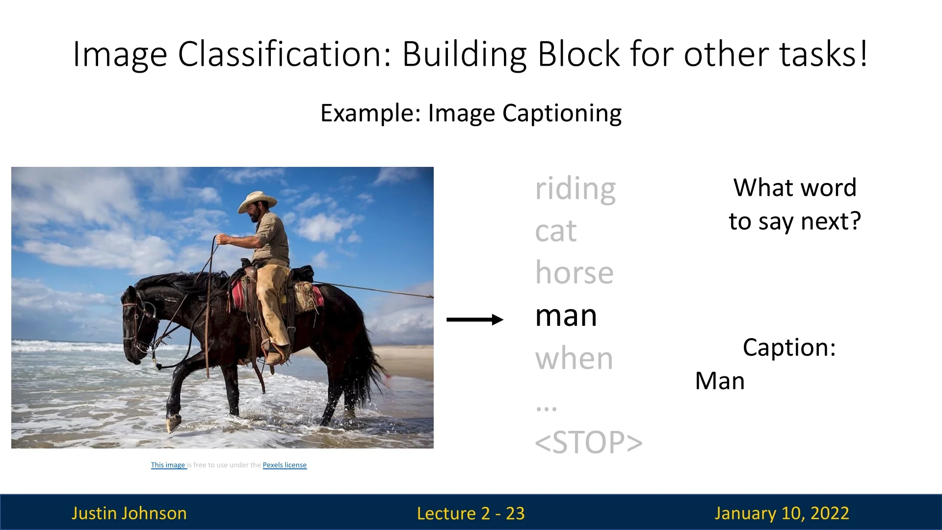
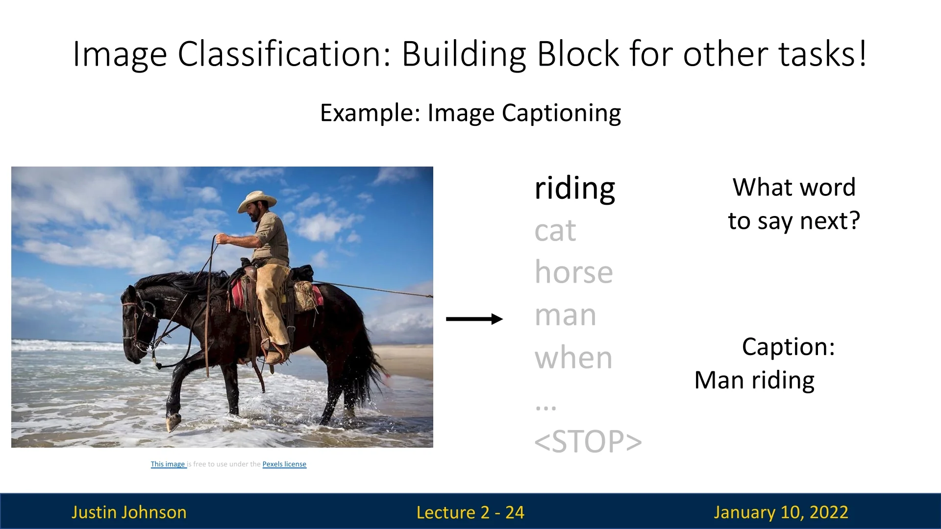
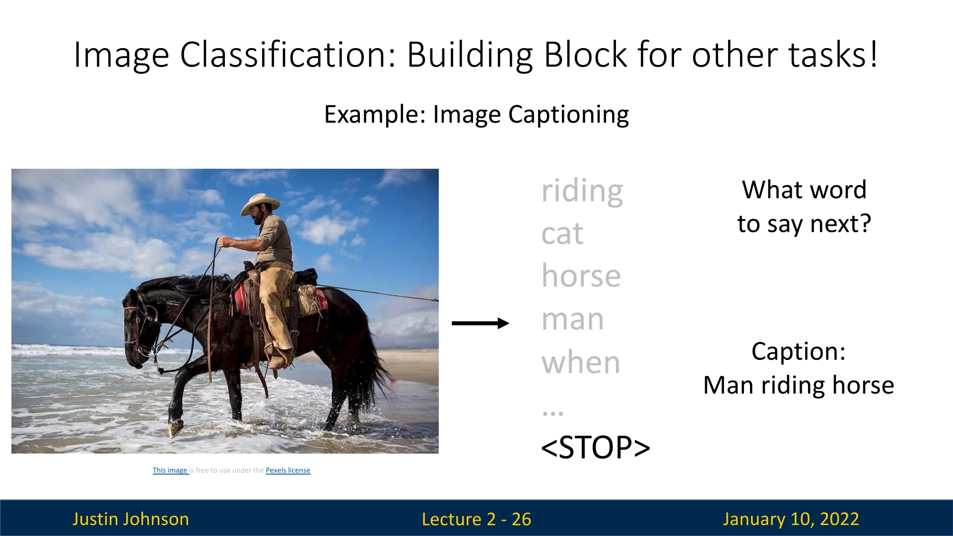
Figure 2.9: Using sliding windows for object detection: classifying regions as background or containing an object.

Figure 2.10: Using sliding windows for object detection: classifying regions containing objects (e.g., person).

2.3.2 Image Captioning

Image captioning involves generating a natural language description of the content in an image, a task that can also be framed as a sequence of classification problems. Given a fixed vocabulary of words, the algorithm determines the most fitting word at each step, effectively performing classification repeatedly until a complete sentence is formed.

For example, starting with an input image, the first classification might yield the word ”man,” followed by ”riding,” then ”horse,” and eventually a ”STOP” token to indicate the end of the caption. This process demonstrates how a robust image classifier can form the backbone of a more complex multimodal task that bridges vision and language.

Figure 2.11: Image captioning as sequential classification: determining the first word (e.g., ”man”).

Figure 2.12: Image captioning as sequential classification: determining the next word (e.g., ”riding”).

Figure 2.13: Image captioning: determining the end of the sentence with a ”STOP” token.

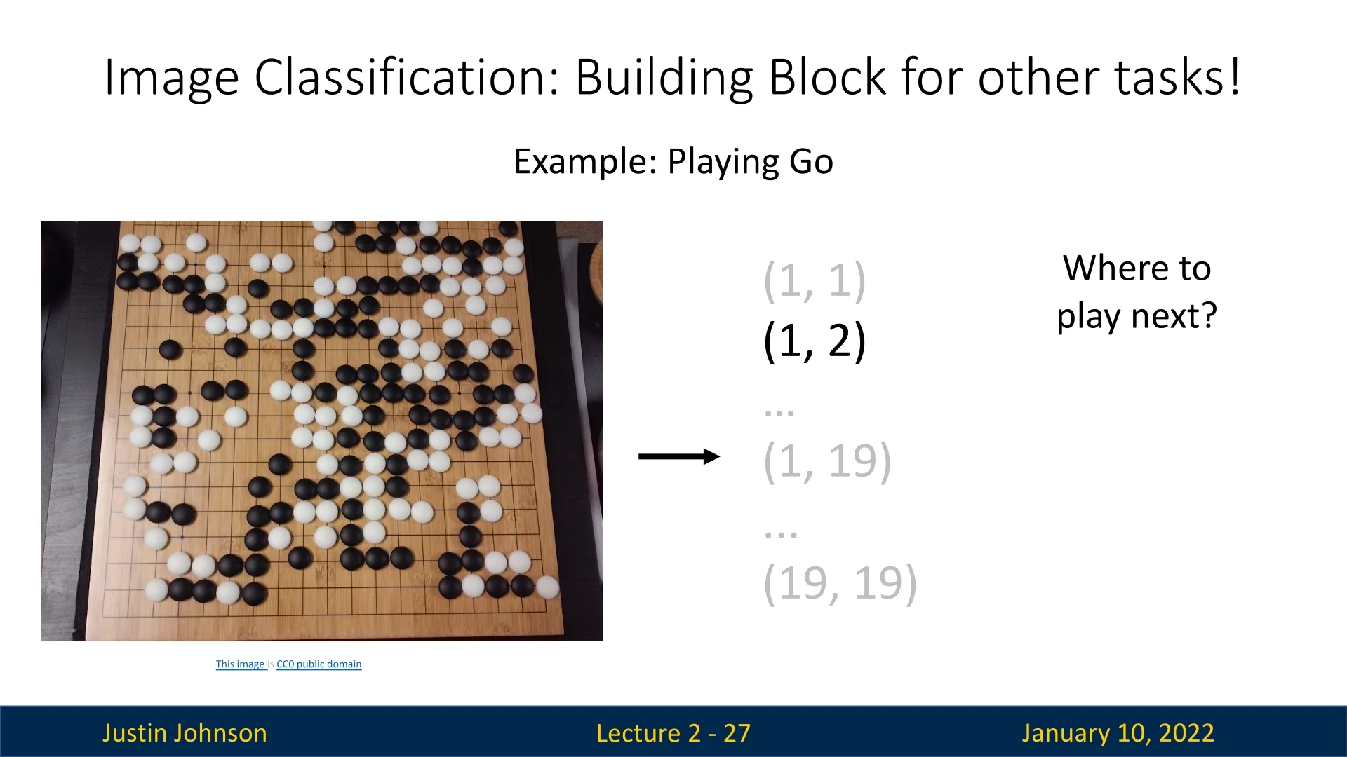
2.3.3 Decision-Making in Board Games

Board games such as Go provide another example of framing a complex task as a classification problem. Each position on the board can be viewed as an input to the algorithm, with the goal of classifying which position is most optimal for the next move. This approach enables algorithms to make strategic decisions by treating each potential move as a classification instance, demonstrating the versatility of image classification as a problem-solving tool.

Figure 2.14: Board games like Go framed as classification problems: determining the optimal next move.

2.3.4 Summary: Leveraging Image Classification

Image classification is not just an isolated task but a fundamental building block for diverse applications in computer vision and artificial intelligence. By leveraging classification in tasks such as object detection, image captioning, and decision-making, researchers have been able to extend its utility and address increasingly complex problems. This underscores the importance of developing robust image classifiers, as they form the foundation for solving more sophisticated challenges.

2.4 Constructing an Image Classifier

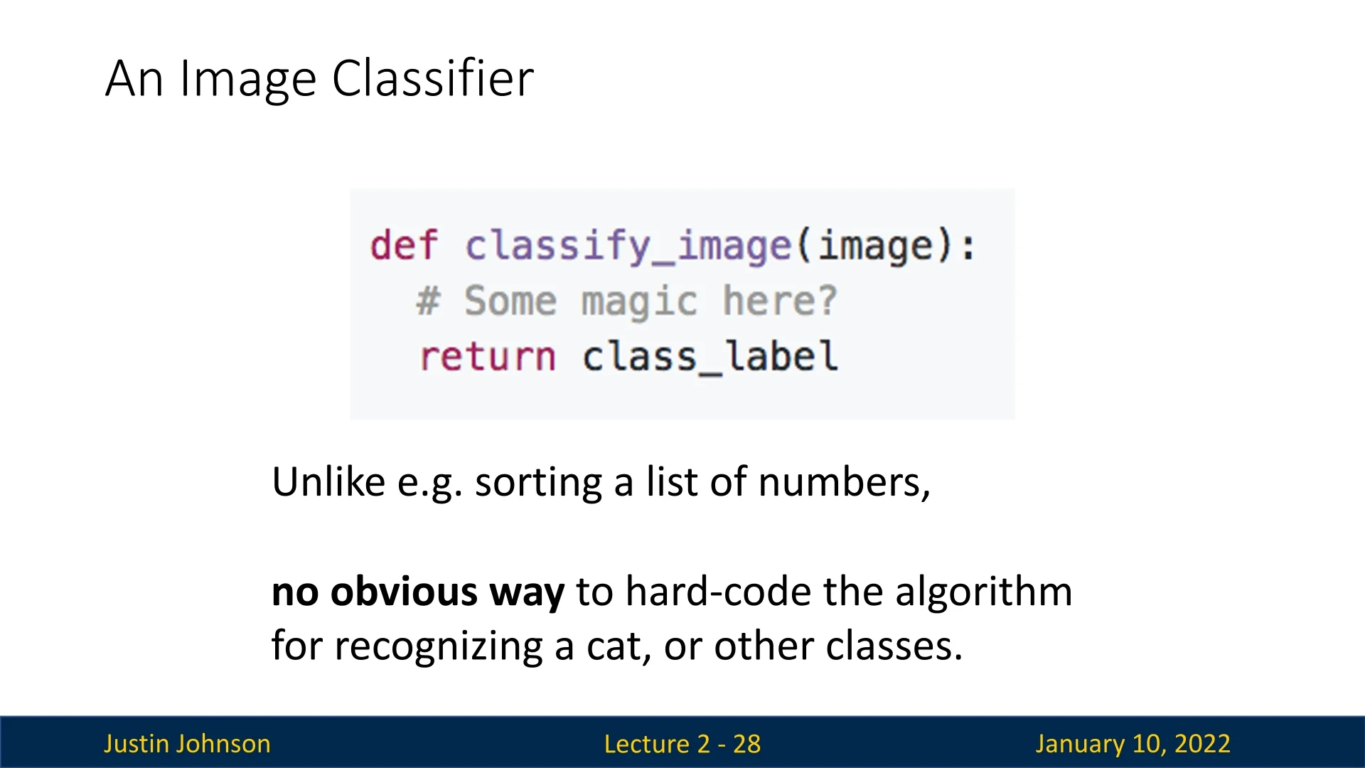
Designing an image classifier is a complex process that cannot be reduced to a simple function like def classify_img(...), which takes an image tensor and directly outputs a category label. This complexity arises from the inherent challenges of translating raw pixel values into meaningful categories. Over time, the field has transitioned from feature-based methods to data-driven approaches, reflecting the increasing complexity of real-world applications.

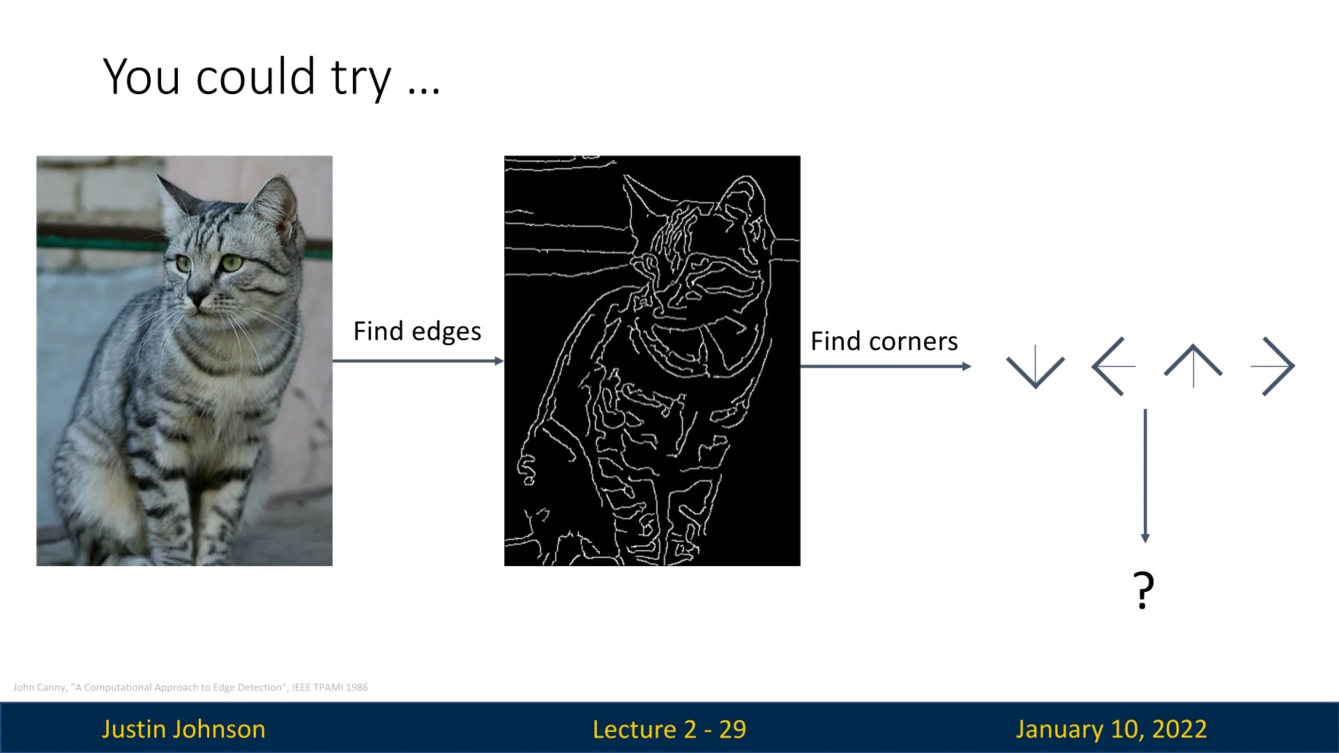
2.4.1 Feature-Based Image Classification: The Classical Approach

Traditional strategies for building an image classifier rely on explicit feature extraction and rule-based classification:

Edge Detection: Algorithms like the Canny Edge Detector [63] are used to identify object boundaries by detecting abrupt changes in pixel intensity.
Keypoint Detection: Techniques such as the Harris Corner Detector [203] locate distinctive features like corners in the image.
Rule-Based Classification: Incorporating human knowledge, explicit rules are devised to classify objects based on extracted features. For example, cats might be identified by triangular ears and whiskers.

While this approach provides a structured framework, it faces critical challenges:

Variability: Real-world objects exhibit significant variations, such as cats with or without whiskers.
Failure Points: Feature detectors often fail under challenging conditions, such as poor lighting or occlusion.
Scalability: Adding new categories requires rewriting rules and redesigning algorithms, limiting adaptability.

Figure 2.15: Attempting to classify images using hard-coded features is highly challenging.

Figure 2.16: Edges and corners as features for classification: an incomplete solution.

2.4.2 From Hand-Crafted Rules to Data-Driven Learning

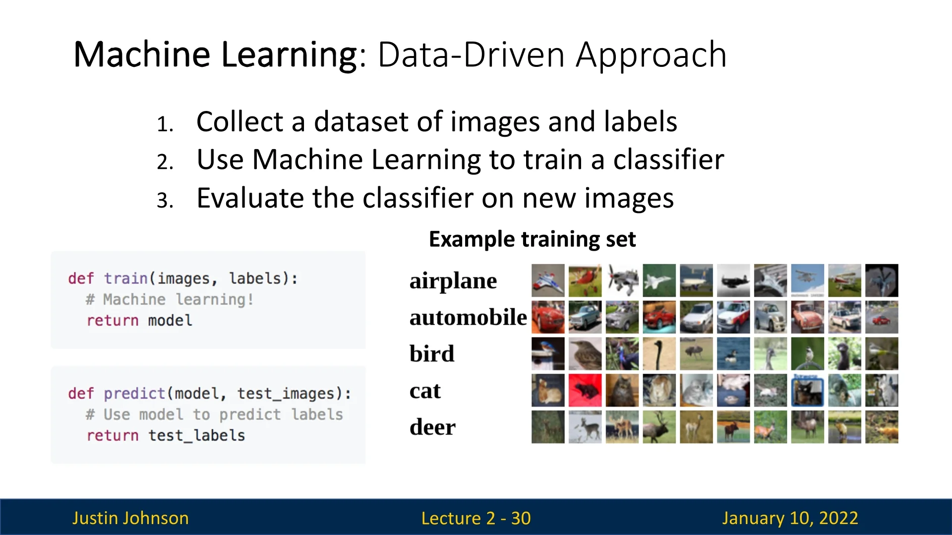
Machine learning revolutionized image classification by replacing manual feature engineering with automated learning from data. This modern approach is defined by three key steps:

1.: Dataset Collection: Collect a large dataset of images and their corresponding human-annotated labels.
2.: Model Training: Train a machine learning model to learn patterns and representations directly from the dataset.
3.: Prediction and Evaluation: Use the trained model to predict labels for unseen images and evaluate performance using metrics like accuracy or log-likelihood.

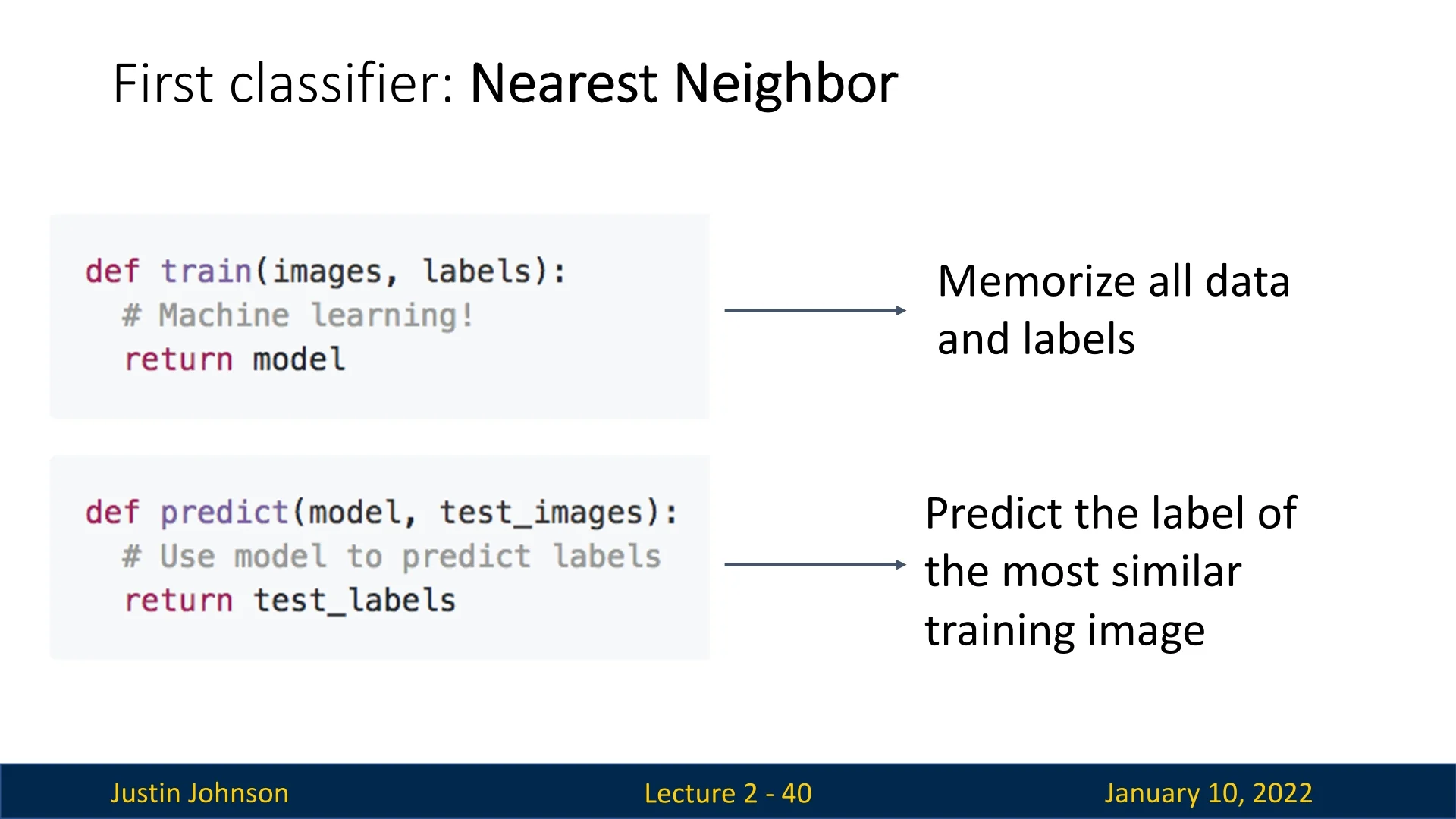
This pipeline, illustrated in Figure 2.17, modularizes the process into two core functions: train(images, labels) and predict(model, test_images).

Figure 2.17: A data-driven pipeline for training and evaluating machine learning-based image classifiers.

2.4.3 Programming with Data: The Modern Paradigm

Data-driven approaches redefine how we ”program” computers. Instead of hard-coding rules, we train models by providing labeled datasets, allowing the algorithm to learn from examples. This shift offers significant advantages:

Scalability: Easily adapts to new categories by adding labeled data.
Robustness: Handles diverse conditions, such as lighting changes and occlusions, without manual adjustments.
Automation: Eliminates the need for explicit, domain-specific rules, making it suitable for complex, real-world tasks.

For example, a data-driven model trained on images of animals learns nuanced distinctions—like fur patterns and body shapes—directly from the data, avoiding the need for manually encoding such rules.

2.4.4 Data-Driven Machine Learning: The New Frontier

Datasets are the foundation of modern machine learning, enabling models to learn directly from examples. Unlike traditional algorithm-driven approaches, where progress relied on better feature engineering, data-driven methods depend on the quality, diversity, and scale of datasets.

Why Data Dominates:

Generalization: Models trained on diverse datasets can generalize to unseen data better than those relying on hand-crafted features.
Flexibility: New tasks and domains require only new data, not redesigned algorithms.
Empirical Strength: Data-driven methods align closely with real-world variability, capturing patterns that are infeasible to encode manually.

The growing emphasis on datasets reflects a paradigm shift in machine learning research, where the quality of data often outweighs incremental algorithmic improvements. This approach empowers models to tackle the complexities of real-world visual data effectively.

In the next section, we delve into the critical role of datasets in machine learning, exploring how they shape the development and performance of image classification models.

2.5 Datasets in Image Classification

Datasets form the backbone of modern machine learning and computer vision, defining the scope and quality of what algorithms can learn. Over the years, datasets in image classification have evolved in scale, complexity, and diversity, shaping the trajectory of the field. In this section, we explore some of the most prominent datasets used in image classification, their characteristics, and their role in advancing research.

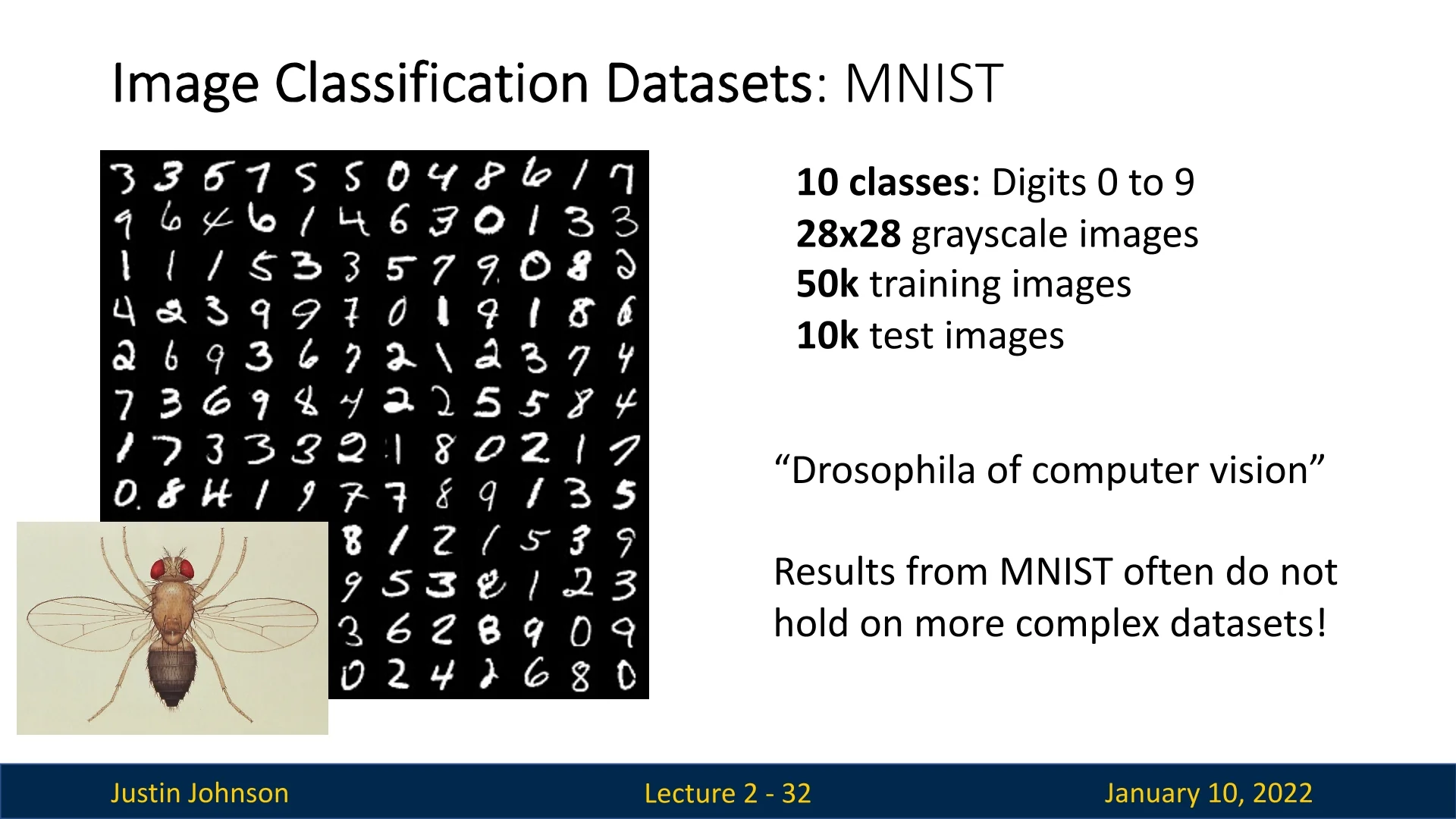
2.5.1 MNIST: The Toy Dataset

The MNIST dataset [316] is one of the earliest and most iconic datasets in machine learning. It consists of \(28 \times 28\) grayscale images of handwritten digits (0–9), making it a 10-class classification problem. With 50,000 training images and 10,000 test images, MNIST has been pivotal in demonstrating the power of early machine learning algorithms.

While MNIST is often referred to as the Drosophila of computer vision, it is considered a toy dataset due to its simplicity and small size. Achieving high accuracy on MNIST does not necessarily translate to success on more complex datasets, limiting its utility in benchmarking modern algorithms.

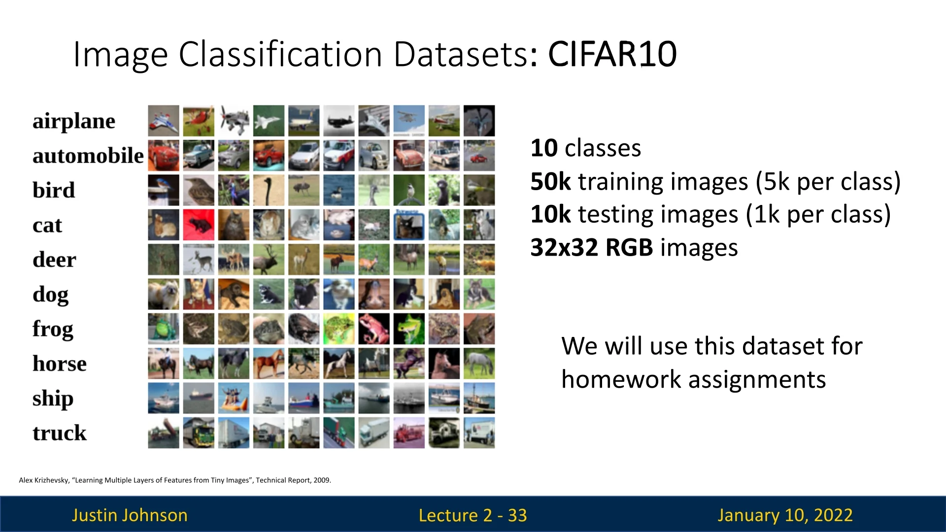
Figure 2.18: MNIST: A dataset of handwritten digits, often used as a toy benchmark.

2.5.2 CIFAR: Real-World Object Recognition

The CIFAR-10 dataset [306] represents a significant step forward in dataset complexity. It contains 10 classes of objects (e.g., airplane, automobile, bird, cat) with \(32 \times 32 \times 3\) RGB images. The dataset includes 50,000 training images (5,000 per class) and 10,000 test images (1,000 per class).

CIFAR-10 strikes a balance between complexity and computational feasibility, making it ideal for research and teaching purposes. In this course, CIFAR-10 is the primary dataset for homework assignments.

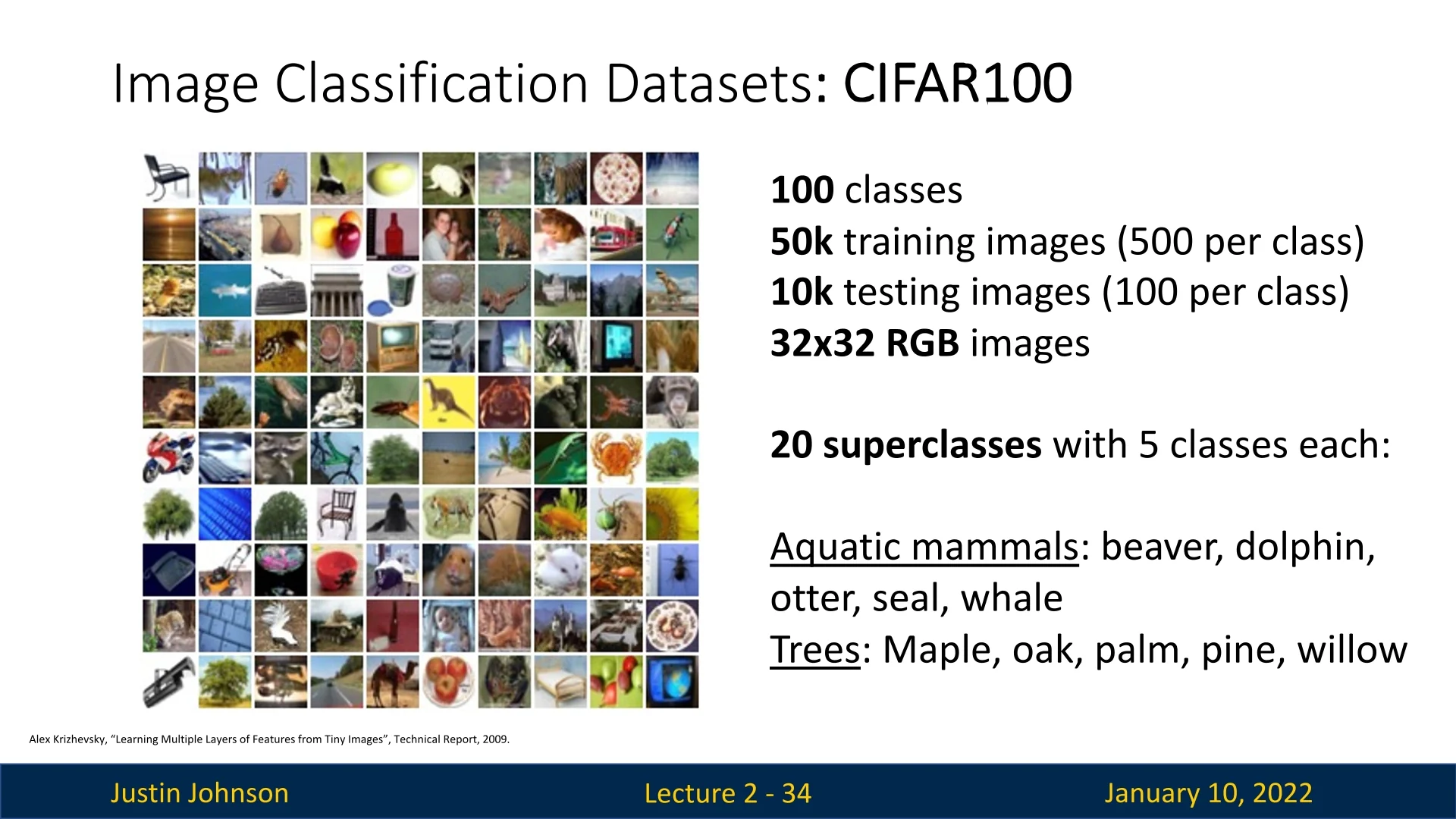
CIFAR-10 has a cousin, CIFAR-100, which has similar statistics but with 100 categories instead of 10. These 100 categories are grouped into 20 superclasses, each containing five finer-grained classes. For example, the Aquatic Animals superclass includes classes like beaver, dolphin, otter, seal, and whale.

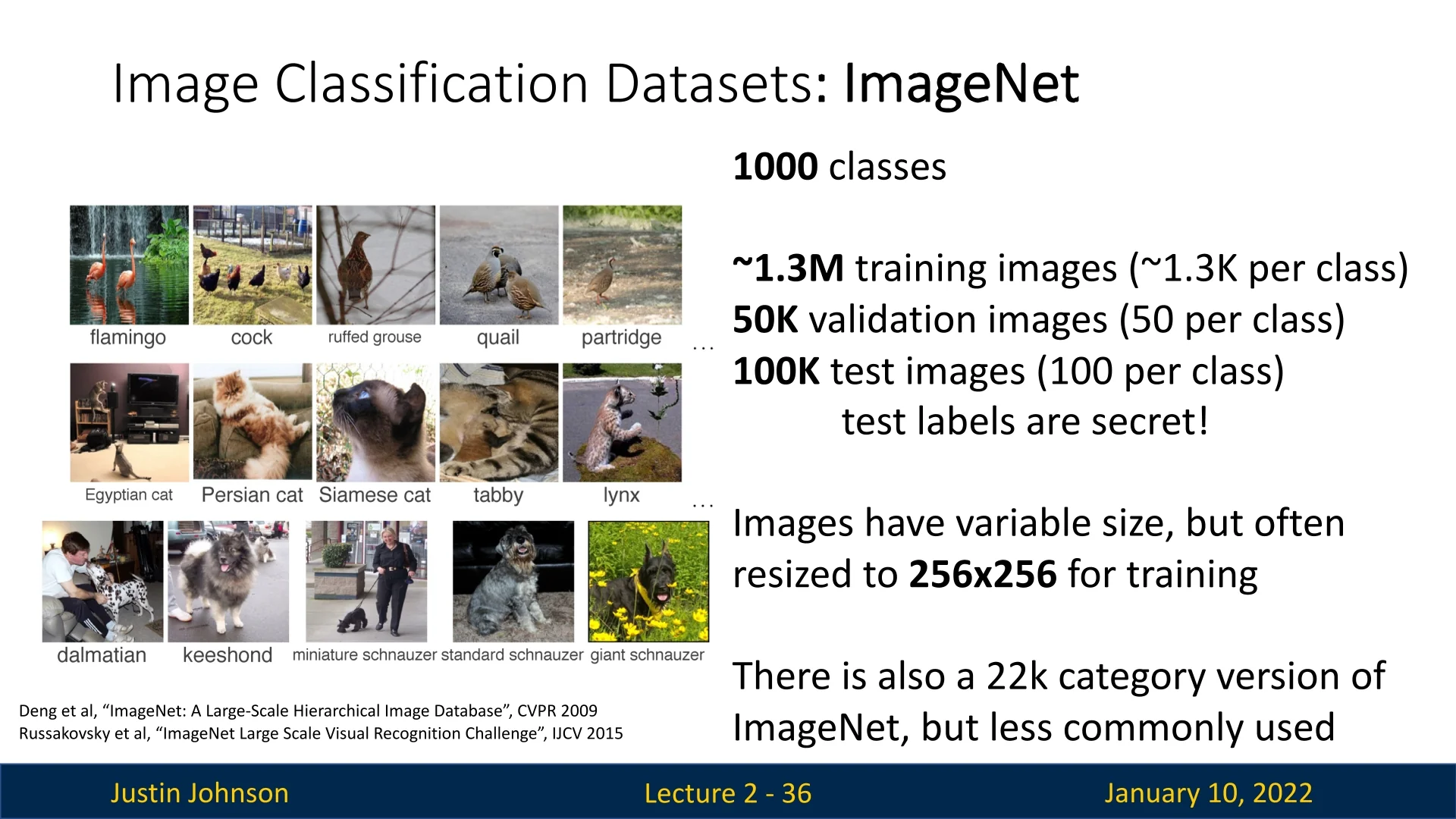
Figure 2.19: CIFAR-10: A dataset for object classification with 10 categories.

Figure 2.20: CIFAR-100: An extension of CIFAR-10 with 100 categories.

2.5.3 ImageNet: The Gold Standard

ImageNet [118] is a cornerstone dataset in computer vision, widely used for benchmarking image classification algorithms. It comprises over 1.3 million training images across 1,000 categories, with approximately 1,300 images per category, alongside 50,000 validation images and 100,000 test images.

Collected from the internet, ImageNet images vary in resolution but are typically resized to \(256 \times 256 \times 3\) for training and evaluation. Its scale and diversity challenge algorithms to generalize effectively, making it ideal for assessing robustness.

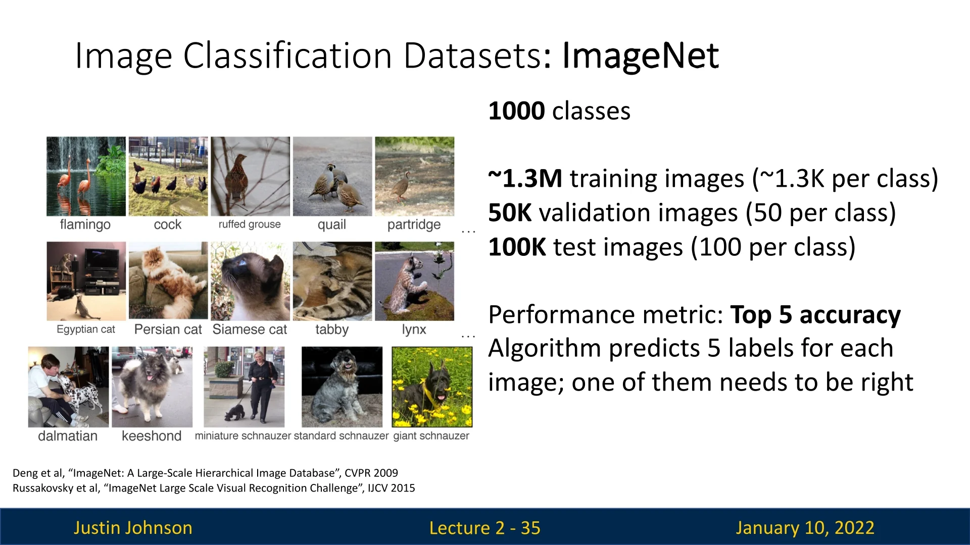
Figure 2.21: ImageNet: A dataset of 1,000 categories pivotal to computer vision progress.

ImageNet’s top-5 accuracy metric allows the algorithm to succeed if the correct label appears among its top 5 predictions, accommodating label ambiguities and noise in the data.

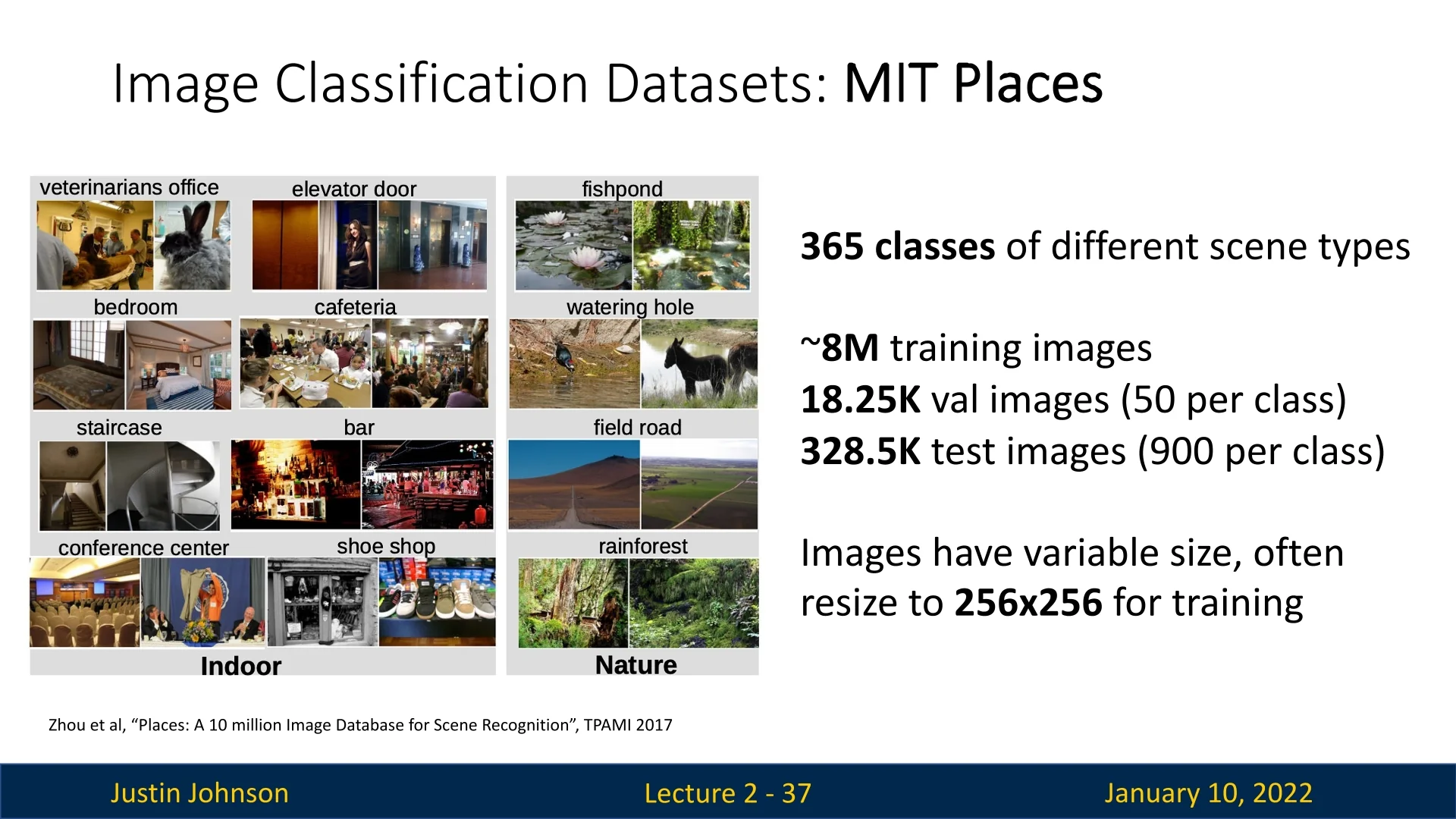
Figure 2.22: ImageNet top-5 accuracy: A widely adopted evaluation metric.

2.5.4 MIT Places: Scene Recognition

While datasets like ImageNet focus on object recognition, the MIT Places dataset [797] emphasizes scene classification, with categories like classrooms, fields, and buildings. This shift from object-centric to scene-centric data broadens the scope of image classification research, enabling algorithms to analyze broader contexts in visual data.

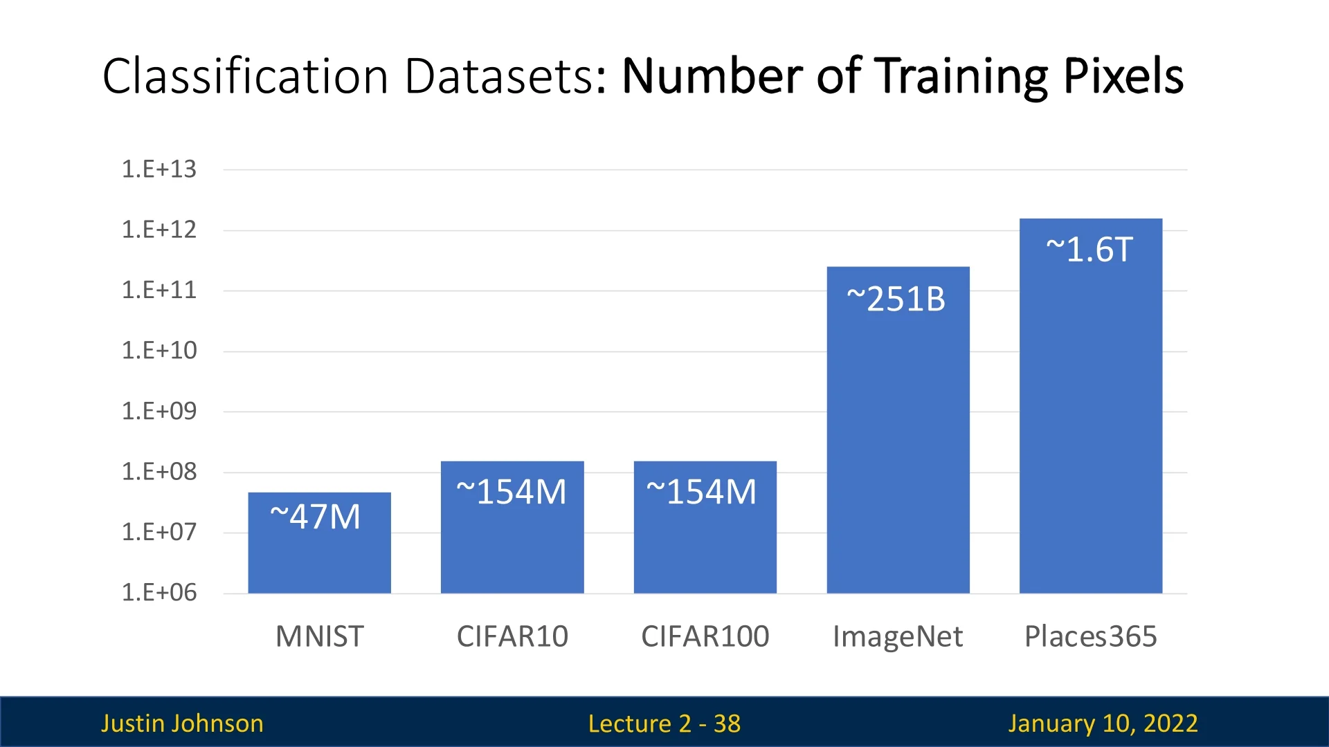
Figure 2.23: MIT Places: A dataset for scene classification, focusing on diverse environmental contexts.

2.5.5 Comparing Dataset Sizes

Figure 2.24 compares the sizes of these datasets in terms of the total number of pixels in their training sets. The y-axis, plotted on a logarithmic scale, reveals a clear trend:

CIFAR is roughly an order of magnitude larger than MNIST.
ImageNet is approximately two orders of magnitude larger than CIFAR.
MIT Places is yet another order of magnitude larger than ImageNet.

This trend reflects the increasing scale of datasets over time, driven by the need for diverse and comprehensive training data. Larger datasets like ImageNet yield more convincing results but demand significant computational resources, which is why smaller datasets like CIFAR remain popular for teaching and prototyping.

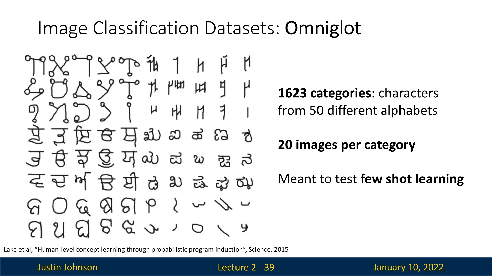
Figure 2.24: Comparing dataset sizes: MNIST, CIFAR, ImageNet, and MIT Places.

2.5.6 Omniglot: Few-Shot Learning

As datasets grow larger, an emerging research direction focuses on learning from limited data. The Omniglot dataset [51] exemplifies this shift by providing only 20 examples per category. Omniglot contains handwritten characters from over 50 different alphabets, emphasizing the challenge of few-shot learning, where algorithms must generalize from minimal examples.

Figure 2.25: Omniglot: A dataset for few-shot learning, with minimal examples per category.

2.5.7 Conclusion: Datasets Driving Progress

Datasets set the limits of model capabilities, with larger and more diverse datasets enabling breakthroughs in image classification. Specialized datasets like Omniglot address challenges like few-shot learning, emphasizing the evolving needs of the field. In data-driven methodologies, the quality and diversity of datasets remain pivotal in advancing computer vision.

2.6 Nearest Neighbor Classifier: A Gateway to Understanding Classification

The Nearest Neighbor (NN) classifier is one of the simplest and most intuitive machine learning algorithms. While seemingly elementary, it introduces key concepts that are foundational to the field of classification. By starting with Nearest Neighbor, we gain a clear understanding of the principles of classification and the practical challenges that arise in real-world scenarios, particularly when working with high-dimensional data.

2.6.1 Why Begin with Nearest Neighbor?

The Nearest Neighbor algorithm serves as an excellent starting point for exploring machine learning for several reasons:

Simplicity: The algorithm’s straightforward design—based on memorizing data and comparing distances—makes it easy to understand and implement.
Foundational Concepts: It introduces the idea of similarity metrics, the importance of distance functions, and the impact of training data quality.
Real-World Limitations: Despite its theoretical appeal, Nearest Neighbor highlights practical challenges such as high inference time, sensitivity to noise, and the curse of dimensionality, motivating the development of more sophisticated algorithms.

By dissecting the Nearest Neighbor classifier, we lay the groundwork for understanding modern approaches to robust classification.

2.6.2 Setting the Stage: From Pixels to Predictions

The fundamental task of a classifier is to assign a category label to an input image, bridging the gap between raw pixel data and semantic meaning. For example, given an image of a cat, the classifier should return the label ”cat.” Achieving this requires a method for comparing the input image to previously seen examples and determining the most appropriate label.

Nearest Neighbor does this by comparing the test image to all training images and selecting the label of the most similar one. This approach, while naive, provides valuable insight into the role of similarity in classification and serves as a stepping stone toward more advanced machine learning models.

The following sections detail the algorithm, its components, and the practical considerations for its use.

2.6.3 Algorithm Description

The Nearest Neighbor classifier operates using two primary methods:

train: Memorizes the training data and corresponding labels without any additional computation.
predict: For a test image, computes the distance to all training images using a similarity function or distance metric. The label of the most similar training image is returned as the prediction.

Figure 2.26: Nearest Neighbor classifier: memorize training data and predict based on the closest match.

2.6.4 Distance Metrics: The Core of Nearest Neighbor

The distance metric determines how ”similar” two images are. The most common choices include:

L1 Distance (Manhattan Distance): Computes the sum of absolute differences between corresponding pixel values: \[ \mbox{L1 Distance} = \sum _{i=1}^{n} |x_i - y_i| \]

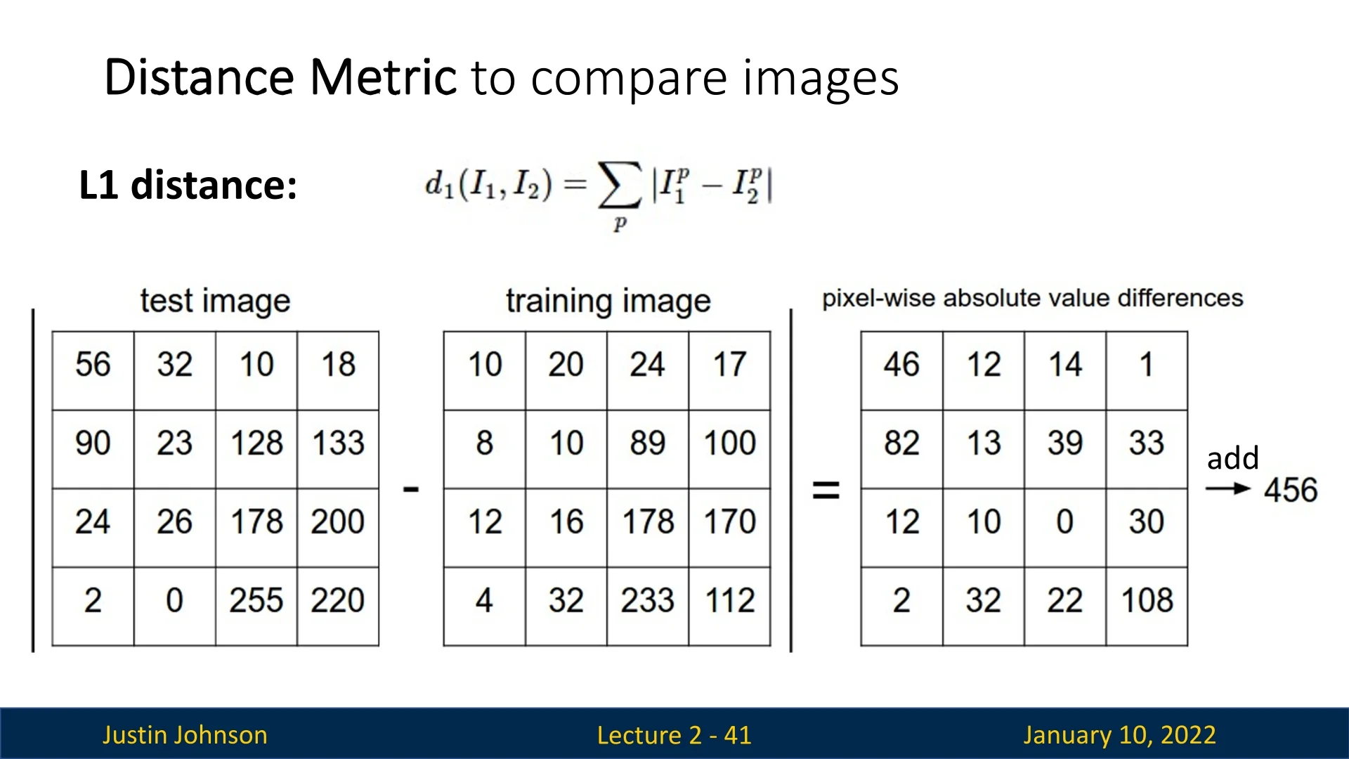
Figure 2.27: L1 distance example: a simple and interpretable metric.
L2 Distance (Euclidean Distance): Computes the root of the sum of squared differences: \[ \mbox{L2 Distance} = \sqrt {\sum _{i=1}^{n} (x_i - y_i)^2} \]
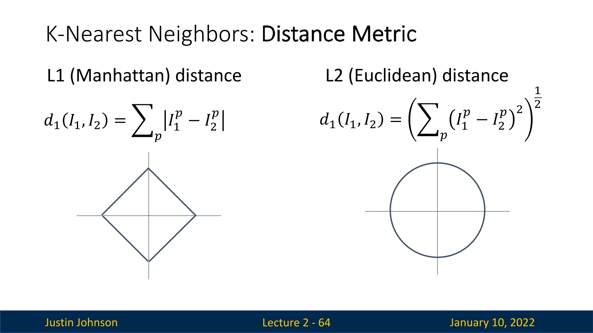
Figure 2.28:
Comparison of L1 and L2 norm constraint regions in two dimensions.
- Left: The L1 norm constraint \( |w_1| + |w_2| = c \) defines a region bounded by four linear segments, forming a diamond. This shape arises because the absolute value function grows linearly and independently in each coordinate, so all points satisfying the constraint lie along lines where the sum of the horizontal and vertical distances equals \( c \).
- Right: The L2 norm constraint \( w_1^2 + w_2^2 = c^2 \) forms a circle, as it includes all points at Euclidean distance \( c \) from the origin \((0,0)\). The quadratic form symmetrically penalizes all directions, yielding a smooth, round boundary.

Figure 2.29: Decision Boundaries for L1 vs. L2 Metrics. In distance-based methods (e.g., nearest neighbors), the choice of distance metric shapes the decision regions:

L1 (Manhattan): Diamond-shaped boundaries (as points at the same L1 distance form axis-aligned corners).

L2 (Euclidean): Circular (or spherical) boundaries, since points equidistant in Euclidean space lie on circles (or spheres).

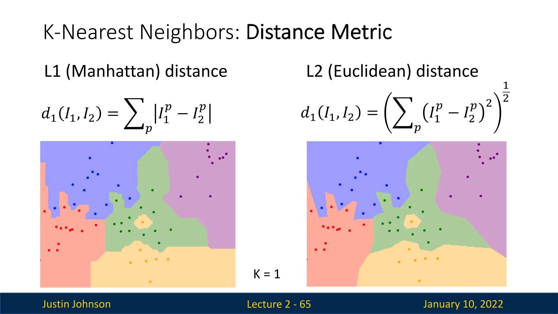
Figure 2.30: Limitations of L1 distance: visually dissimilar objects with similar colors may be incorrectly classified.

Each metric produces different decision boundaries, as shown in Slide 2.29. However, these pixel-based metrics often fail to capture semantic similarity. For instance, as demonstrated in Slide 2.30, visually dissimilar objects with similar colors (e.g., a ginger cat and an orange frog) may appear ”close” under L1 or L2 distance.

2.6.5 Extending Nearest Neighbor: Applications Beyond Images

While the Nearest Neighbor classifier is typically discussed in the context of image classification, its principles can be extended to other domains and data types, provided a suitable distance function is defined.

Using Nearest Neighbor for Non-Image Data

One compelling example of Nearest Neighbor applied to non-image data involves the analysis of academic papers. In this context, similarity between documents is measured using TF-IDF similarity (Term Frequency–Inverse Document Frequency). This metric captures the importance of words in a document relative to a collection of documents, emphasizing unique and meaningful terms while downplaying common ones like “the” or “and.”

Term Frequency (TF): Measures how often a term appears in a document, providing a sense of relevance within that document.
Inverse Document Frequency (IDF): Reduces the weight of terms that appear frequently across many documents, as these are less likely to be unique or significant.
TF-IDF Score: Combines TF and IDF to assign a weight to each term in a document, capturing its importance within a specific context.

Academic Paper Recommendation Example

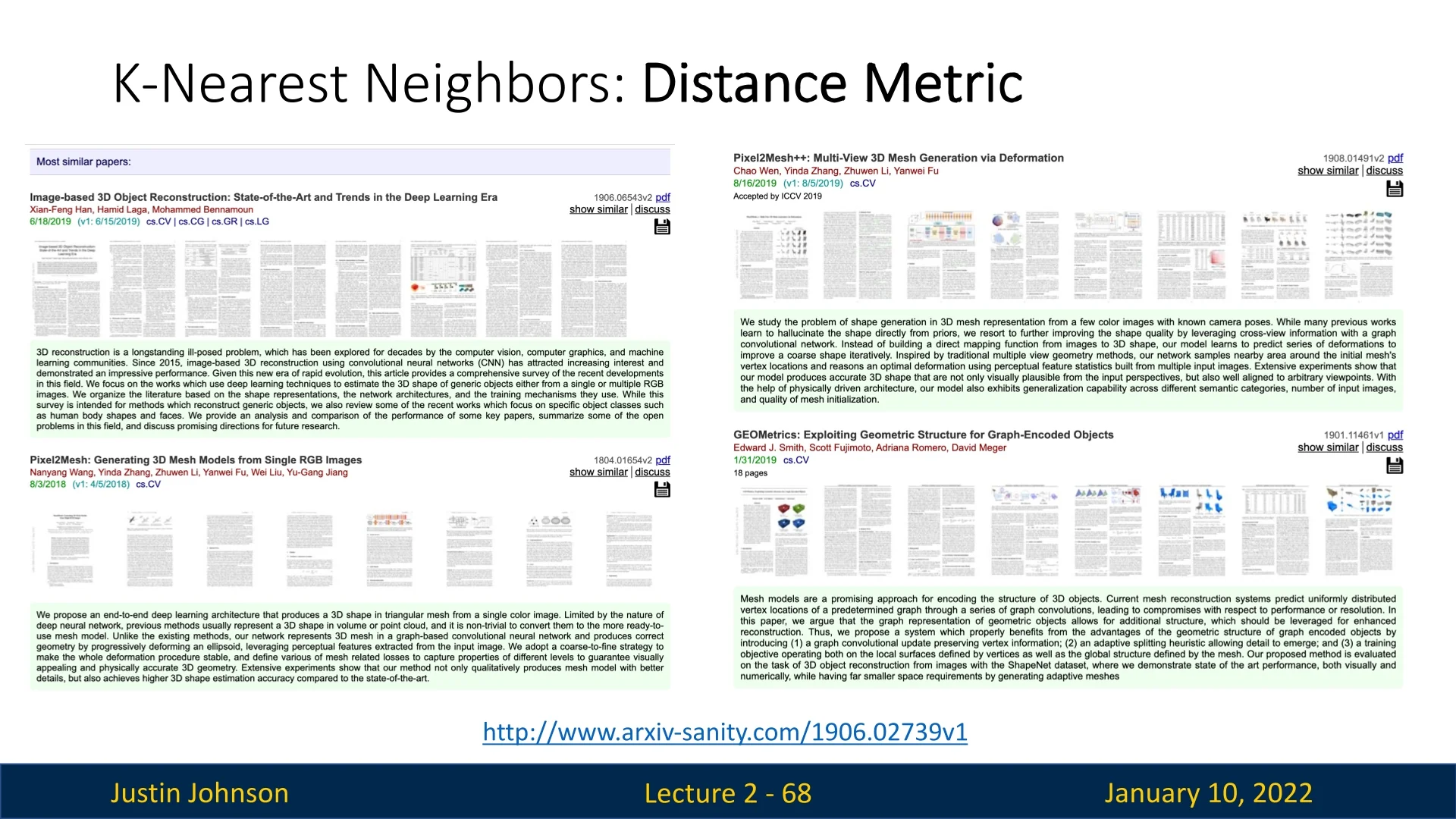
Figure 2.31: Nearest Neighbor using TF-IDF similarity for academic paper recommendations.

Using TF-IDF scores, we can represent each academic paper as a feature vector. Nearest Neighbor can then be employed to find similar papers by comparing these vectors in feature space. As illustrated in Figure 2.31, querying for a specific paper returns its closest neighbors based on semantic similarity.

In practice, we often retrieve not just the single nearest document, but the top \(k\) most similar papers. Here, \(k\) denotes the number of neighbors returned (for example, \(k=5\) yields the five most similar papers). This approach is commonly referred to as \(k\)-Nearest Neighbors.

This example highlights the flexibility of Nearest Neighbor for non-image data. By choosing an appropriate similarity metric such as TF-IDF, we can uncover meaningful relationships between documents and build effective recommendation systems.

Key Insights

The versatility of Nearest Neighbor and K-means clustering stems from their reliance on distance metrics. This allows these algorithms to adapt to various applications, including:

Recommending academic papers based on content similarity.
Grouping documents into clusters for topic modeling.
Analyzing user behavior in recommendation systems.

This flexibility makes these methods powerful tools not only in computer vision but also in broader machine learning contexts.

2.6.6 Hyperparameters in Nearest Neighbor

The performance of the Nearest Neighbor classifier depends on two hyperparameters:

k: The number of nearest neighbors.
Distance Metric: Determines how similarity between images is computed.

Selecting the best hyperparameters is challenging because they cannot be directly learned from training data.

Some strategies we can think of to select model hyperparameters include:

1.

Using the Entire Dataset: Selecting hyperparameters that optimize performance on the training set is misleading. For example, \(k=1\) will perform good in this case, and may lead to overfitting and poor generalization.

2.

Train-Test Split Without Validation: While better than the previous method, this approach lacks a clear mechanism to evaluate model performance on unseen data.

3.

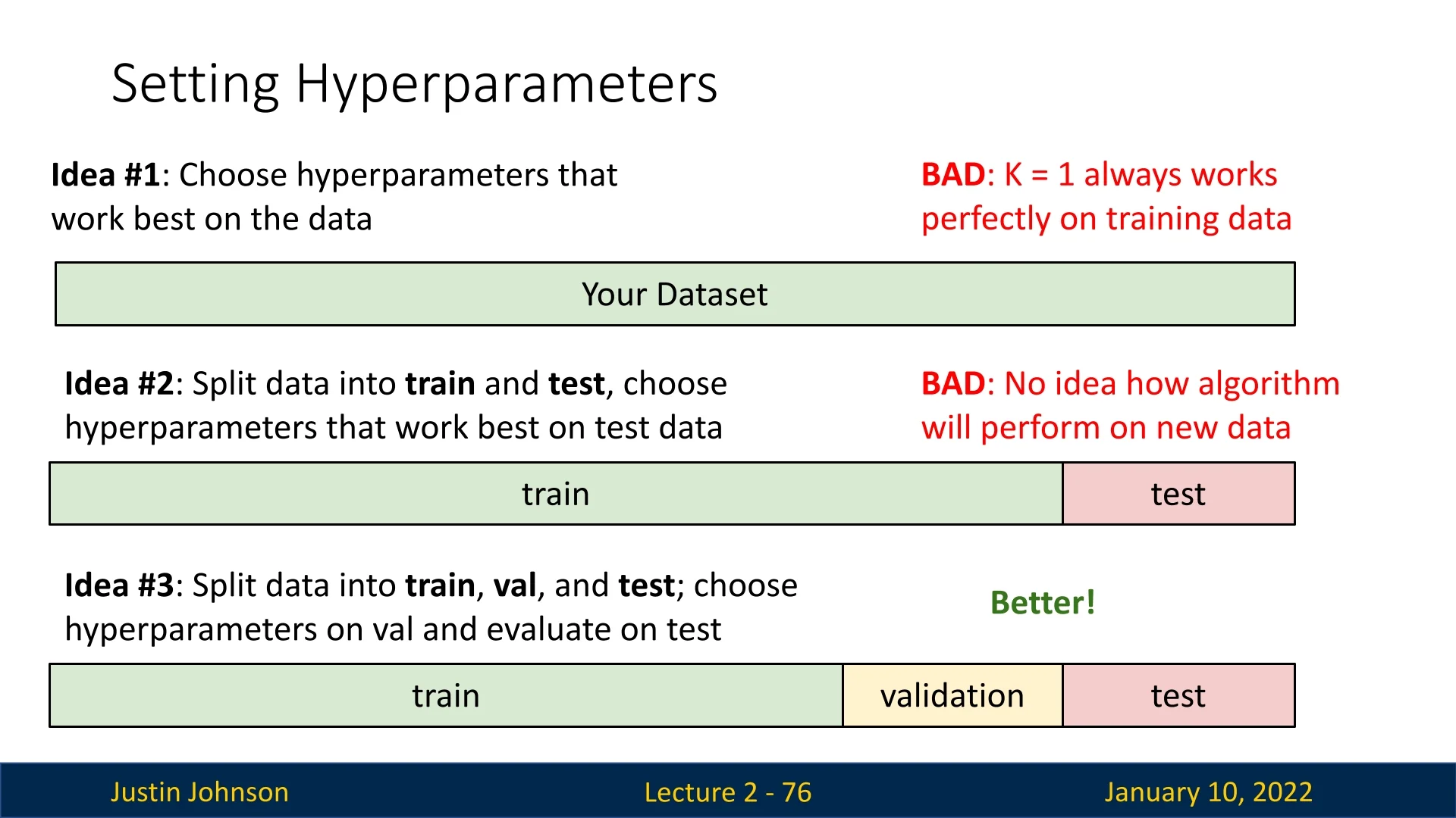
Train-Validation-Test Split: The recommended practice is to split data into three sets:

Training Set: Used for fitting the model.
Validation Set: Helps tune hyperparameters and assess overfitting.
Test Set: Evaluates the final model after all hyperparameters are fixed.

The test set is only evaluated once, at the very end, as emphasized in Slide 2.32. Although scary (as we tend to develop an algorithm spending a lot of time) as the resultant algorithm may prove to be ineffective on the test data, this is the correct data hygiene approach. The test set should only be used once, and near the end of the development.

Figure 2.32: Train-validation-test split for robust evaluation.

2.6.7 Cross-Validation

For smaller datasets, k-fold cross-validation is a widely used strategy for reliable model evaluation and hyperparameter tuning. Note: this method should not be confused with k-nearest neighbors; it refers to a technique for assessing a model’s generalization ability.

In k-fold cross-validation, the available dataset is first split into two parts:

A dedicated test set, held out and untouched until the final evaluation.
A training+validation set, which is used for model selection and cross-validation.

This training+validation set is then partitioned into \(k\) equally sized folds. For each of the \(k\) iterations, one fold is treated as a temporary validation set, and the remaining \(k-1\) folds are used for training.

The process is repeated \(k\) times such that every fold serves as validation exactly once. The resulting performance metrics (e.g., accuracy or loss) are averaged across the \(k\) runs to produce a more stable and reliable estimate of model quality.

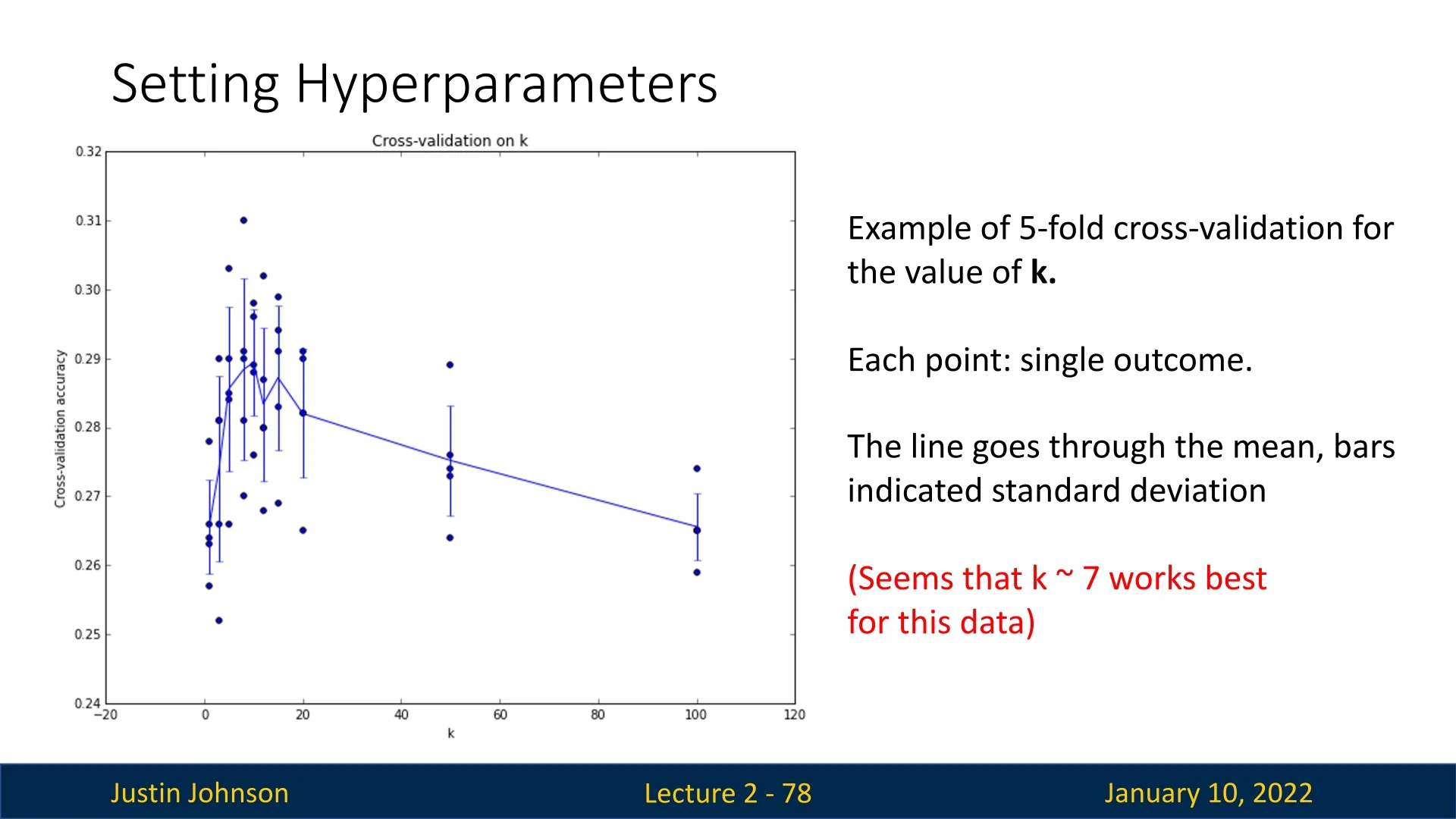
Figure 2.33: Cross-validation accuracy for different values of \(k\). Each dot represents an individual trial, and the mean accuracy across folds is shown by the line. In this example, \(k = 7\) yields the highest average validation performance, so it is selected.

This method provides a robust mechanism for hyperparameter selection and model comparison, particularly when limited data makes a single train-validation split unreliable. It is important to emphasize that the test set is never used during cross-validation. It remains completely separate and is reserved for the final, unbiased evaluation of the trained model, only after all tuning is complete.

While cross-validation is computationally feasible and valuable for smaller datasets or shallow models, it becomes impractical for large-scale datasets or deep learning models due to the repeated training involved. For such cases, a single train-validation split is typically used during training instead (often paired with mechanisms such as early stopping).

2.6.8 Implementation and Complexity

The simplicity of Nearest Neighbor allows for a straightforward implementation:

Figure 2.34: train method: Memorizing training data.

Figure 2.35: predict method: Computing similarity and predicting the closest label.

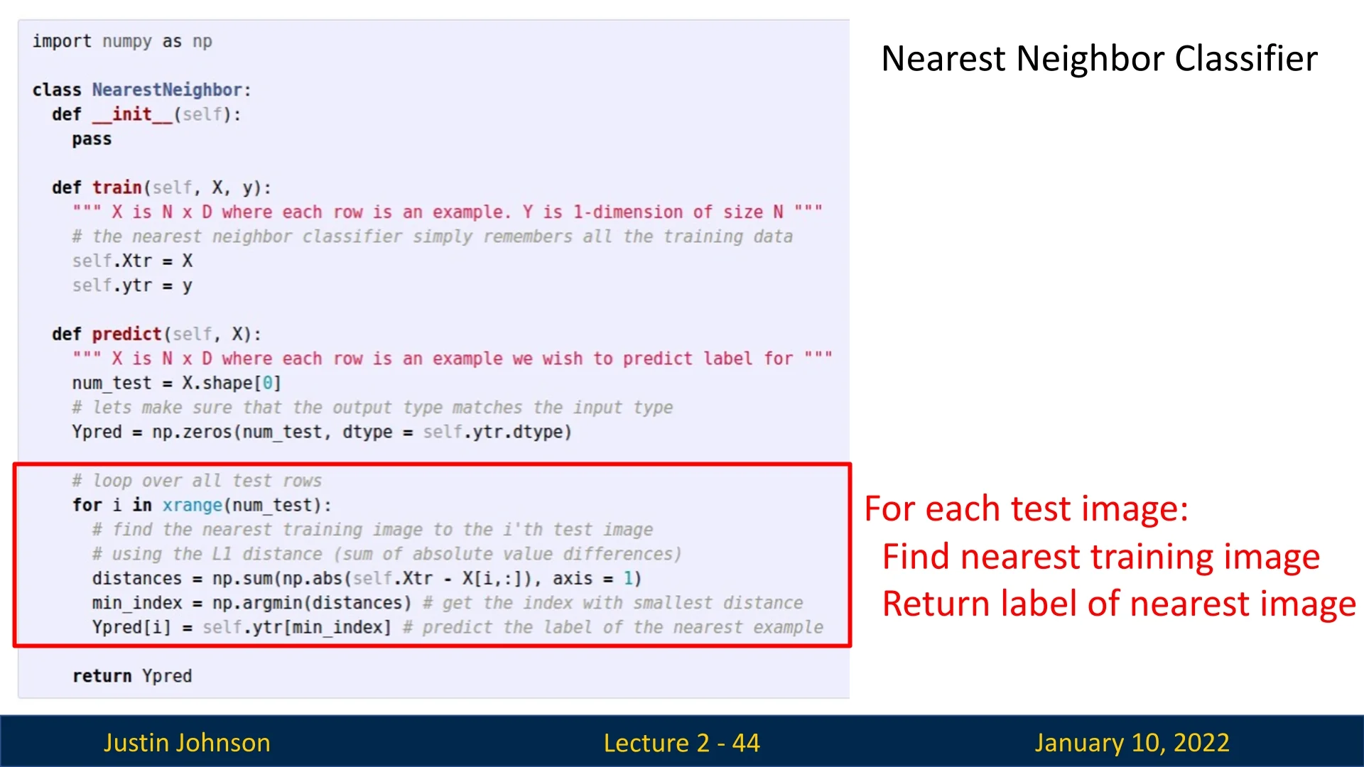
Complexity:

Training: \(O(1)\), as it simply stores the data.
Inference: \(O(n)\), as every test image is compared against all \(n\) training images. This makes inference computationally expensive, particularly for large datasets.

Faster or approximate versions of Nearest Neighbor exist, taking advantage of spatial data structures like KD-trees to accelerate the search process.

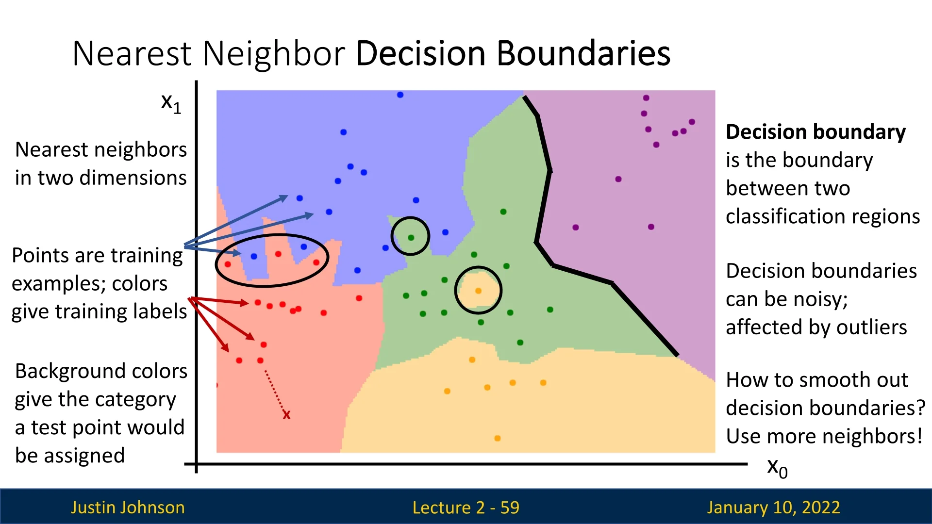
2.6.9 Visualization of Decision Boundaries

Decision boundaries illustrate the regions in the input space assigned to different classes. For a 2D toy dataset, the decision boundaries of Nearest Neighbor are highly irregular and sensitive to outliers.

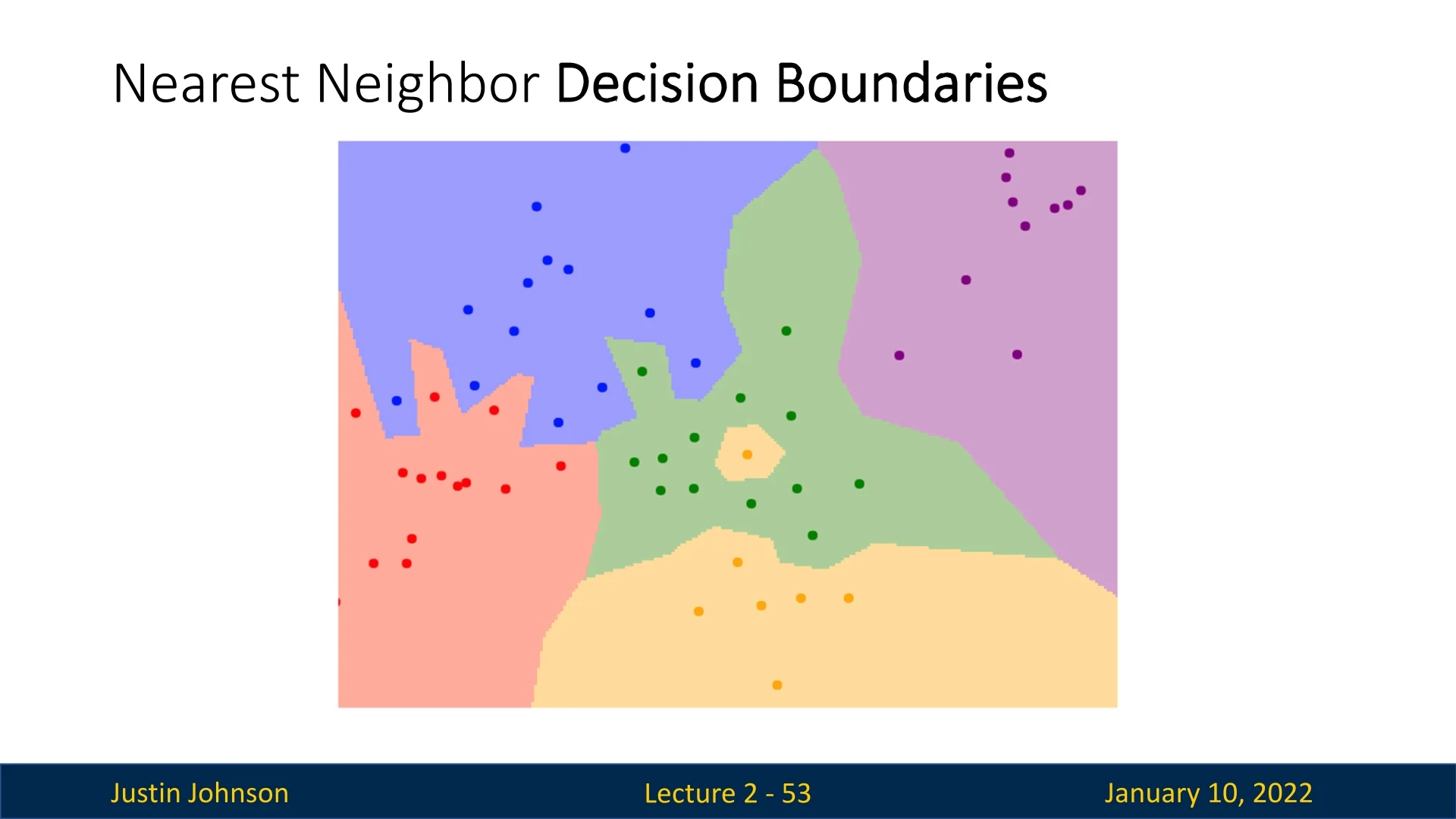
Figure 2.36: Decision boundaries for Nearest Neighbor on a 2D dataset.

Outliers can create ”islands” of incorrect predictions, as shown in Slide 2.37. This sensitivity makes \(k=1\) particularly problematic.

Figure 2.37: Outliers disrupting decision boundaries in Nearest Neighbor classification.

2.6.10 Improvements: k-Nearest Neighbors

The k-Nearest Neighbors (k-NN) algorithm improves upon Nearest Neighbor by considering the \(k\) closest neighbors and using a majority vote to determine the predicted label. This smooths decision boundaries and reduces the impact of outliers.

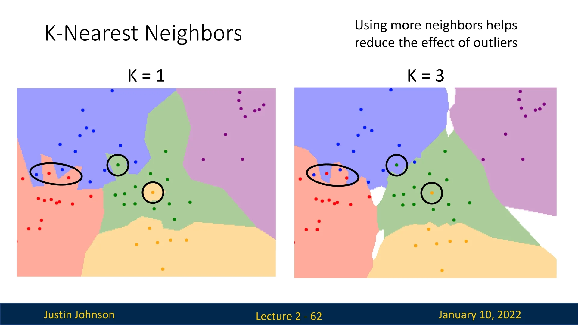
Figure 2.38: k-Nearest Neighbors (\(k=3\)): Smoother decision boundaries and reduced outlier influence.

However, k-NN introduces challenges such as ties between classes when \(k>1\). These ties can be resolved using heuristics like selecting the label of the nearest neighbor or weighting votes by distance.

2.6.11 Limitations and Universal Approximation

With infinite training data, Nearest Neighbor can theoretically approximate any function. This is due to its capacity to memorize and interpolate training examples. As more points are added, the decision boundaries become increasingly fine-grained, capturing ever subtler data patterns.

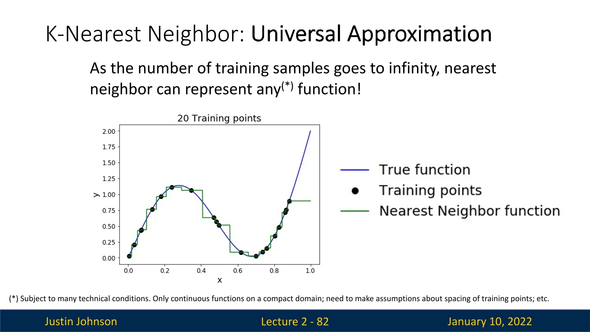
Figure 2.39: A step towards a dense coverage with Nearest Neighbor.

However, the practicality of this property is severely limited by the curse of dimensionality. For high-dimensional data, the number of required training samples grows exponentially. For example:

In \(2\) dimensions, uniform coverage requires \(4^2 = 16\) points.
In \(3\) dimensions, \(4^3 = 64\) points are necessary.
For even modestly sized images like \(32 \times 32\), the number of possible binary images is astronomical: \(2^{32 \times 32} \approx 10^{308}\), far exceeding the number of elementary particles in the visible universe (\(\approx 10^{97}\)).

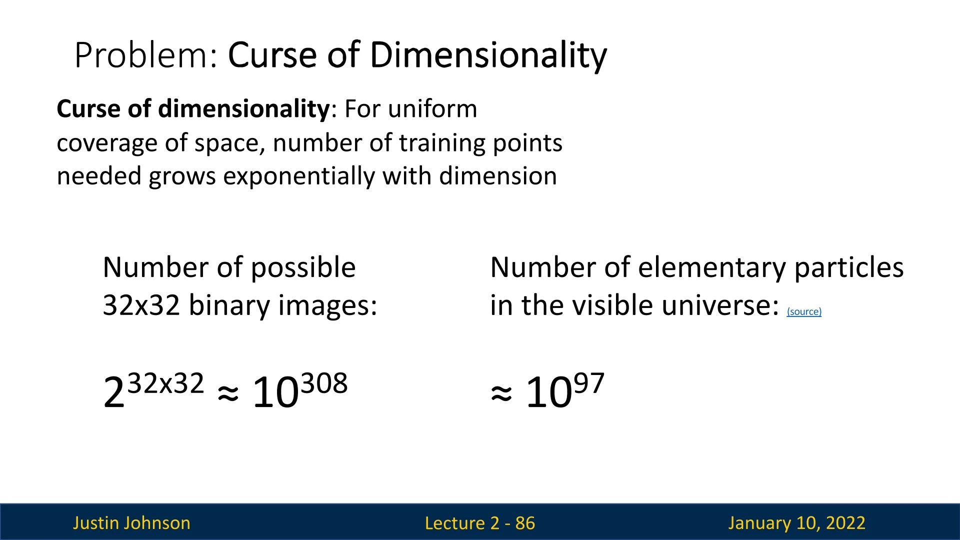
Figure 2.40: The curse of dimensionality: limitations of KNN in high-dimensional spaces.

This exponential growth renders dense coverage impossible for real-world datasets, as highlighted in Slide 2.40. Furthermore, we are often dealing with real-valued RGB images of even higher resolutions, adding to the complexity.

2.6.12 Using CNN Features for Nearest Neighbor Classification

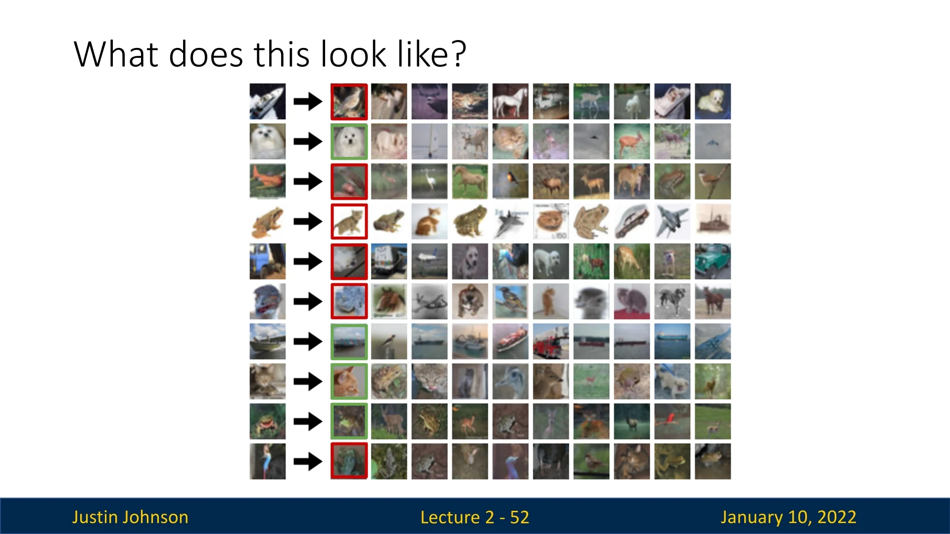
Pixel-based distance metrics, such as L1 and L2 distances, often fail to capture semantic similarity. As highlighted in Slide 2.30, objects with similar pixel intensities, such as a ginger cat and an orange frog, may be incorrectly classified as similar despite their clear visual and categorical differences. This limitation underscores the need for more sophisticated representations that go beyond raw pixel comparisons.

A promising solution is to replace raw pixel distances with feature distances derived from convolutional neural networks (CNNs). CNNs are adept at capturing higher-level semantic information by learning hierarchical feature representations directly from data. These features can effectively bridge the gap between low-level pixel values and meaningful object categories, enabling Nearest Neighbor classifiers to make more informed predictions, bridging the semantic gap L1 or L2 metrics applied to raw pixel values face.

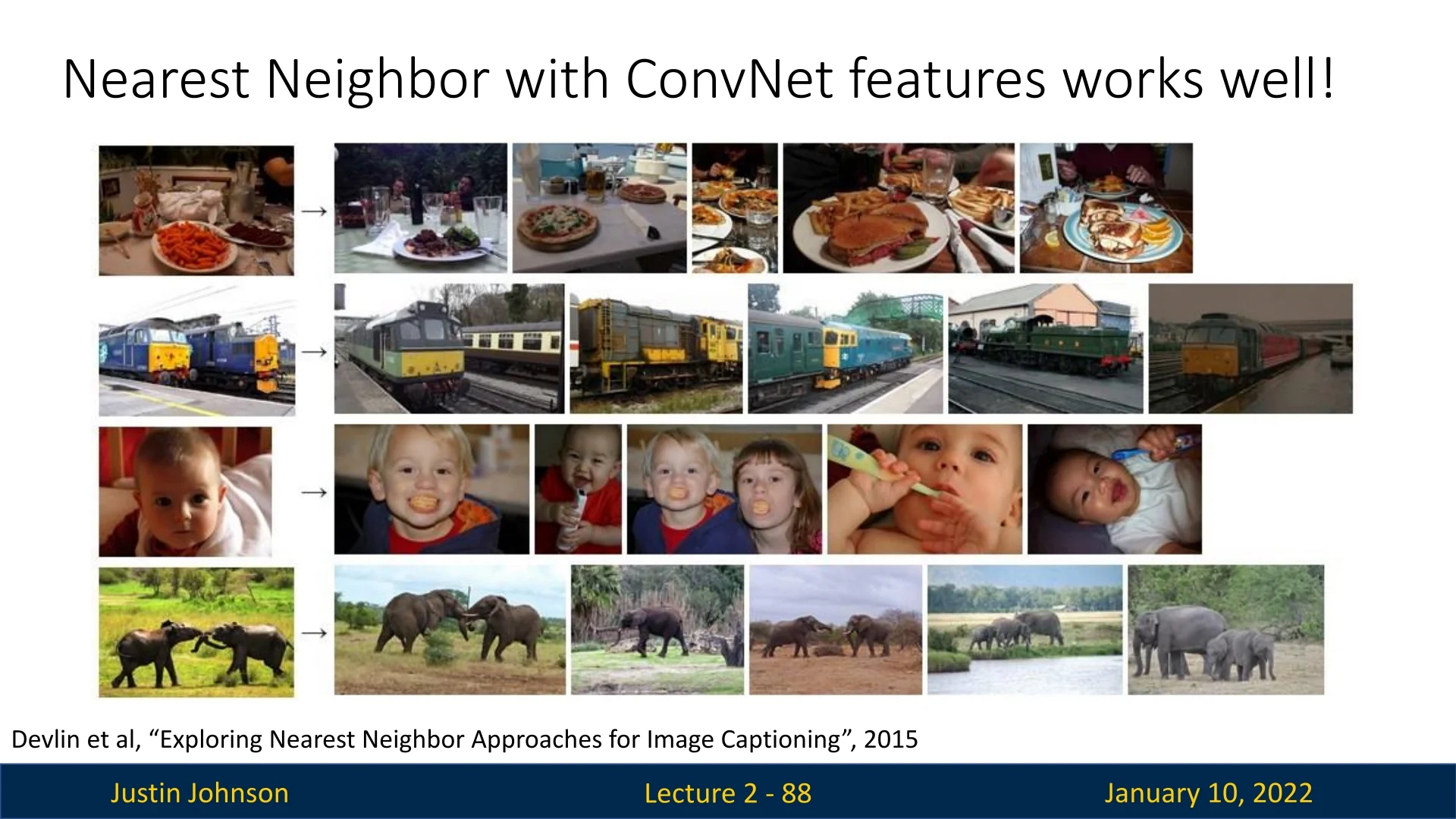
Figure 2.41: Nearest Neighbor with CNN features: improved semantic similarity.

Slide 2.41 demonstrates the effectiveness of this approach, showcasing improved classification performance when CNN-derived features are paired with Nearest Neighbor classifiers. By leveraging these features, the algorithm becomes more robust to variations in lighting, scale, and viewpoint, which are challenging for pixel-based metrics to handle.

This method has proven particularly effective in various tasks, including image captioning. In their work [119], Devlin et al. (2015) proposed an approach that combines Nearest Neighbor with CNN features to generate captions for images. The algorithm retrieves the most similar image from the training set (based on CNN feature similarity) and reuses its caption as the prediction. While simplistic, this method delivered coherent and contextually relevant captions.

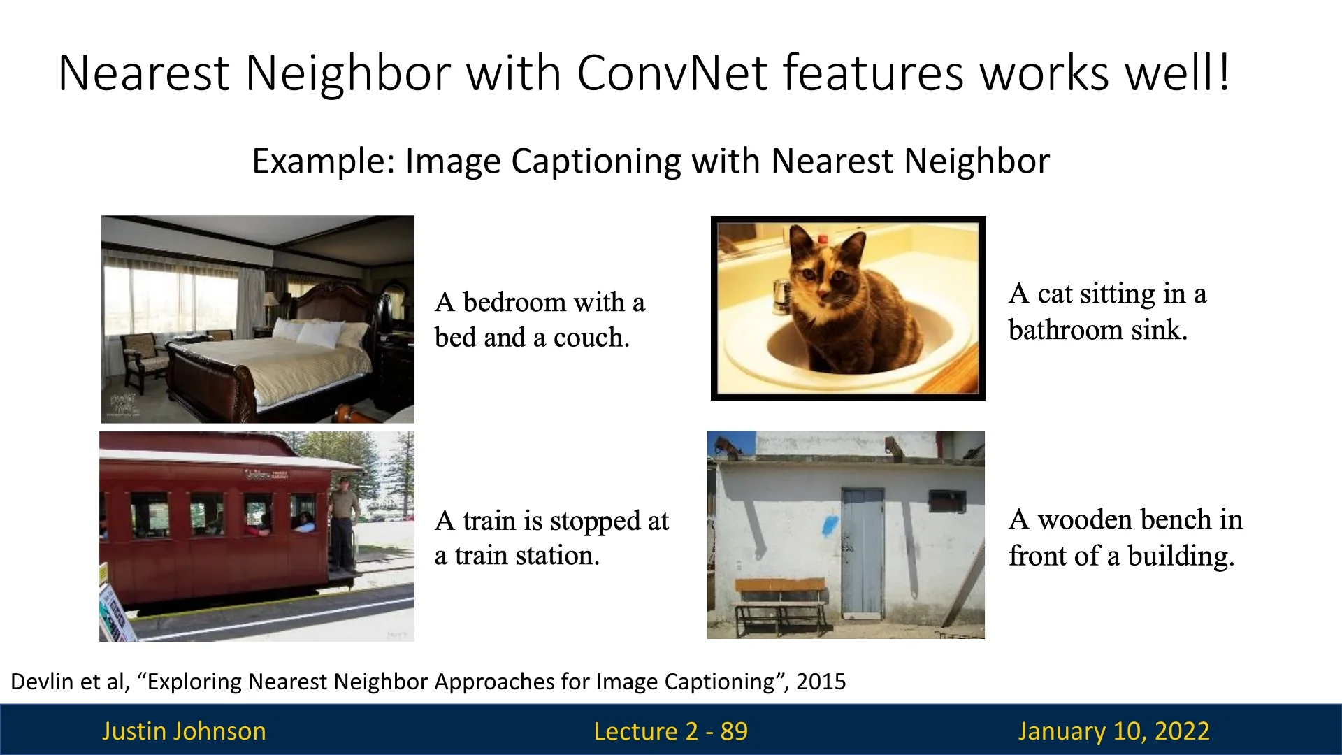
Figure 2.42: Nearest Neighbor captioning: retrieving captions from the closest matching image.

These are examples as to how Nearest Neighbor classifiers, when augmented with learned features, can tackle complex tasks beyond basic classification.

2.6.13 Conclusion: From Nearest Neighbor to Advanced ML Frontiers

The Nearest Neighbor classifier highlights the balance between simplicity and capability, offering theoretical guarantees such as universal function approximation. However, its reliance on raw pixel metrics limits its practical applications, particularly in high-dimensional spaces. By incorporating feature representations from CNNs, Nearest Neighbor classifiers can overcome many of these limitations, improving performance in tasks ranging from image classification to captioning. These advancements pave the way for exploring even more sophisticated machine learning algorithms and architectures in subsequent sections.