Lecture 16: Recurrent Networks
16.1 Introduction to Recurrent Neural Networks (RNNs)
Many real-world problems involve sequential data, where information is not independent but instead follows a temporal or ordered structure. Traditional neural networks, such as fully connected (FC) networks and convolutional neural networks (CNNs), assume that inputs are independent of each other, making them ineffective for tasks where past information influences future outcomes. Recurrent Neural Networks (RNNs) are specifically designed to handle such problems by incorporating memory through recurrent connections, enabling them to process sequences of variable length.
16.1.1 Why Study Sequential Models?
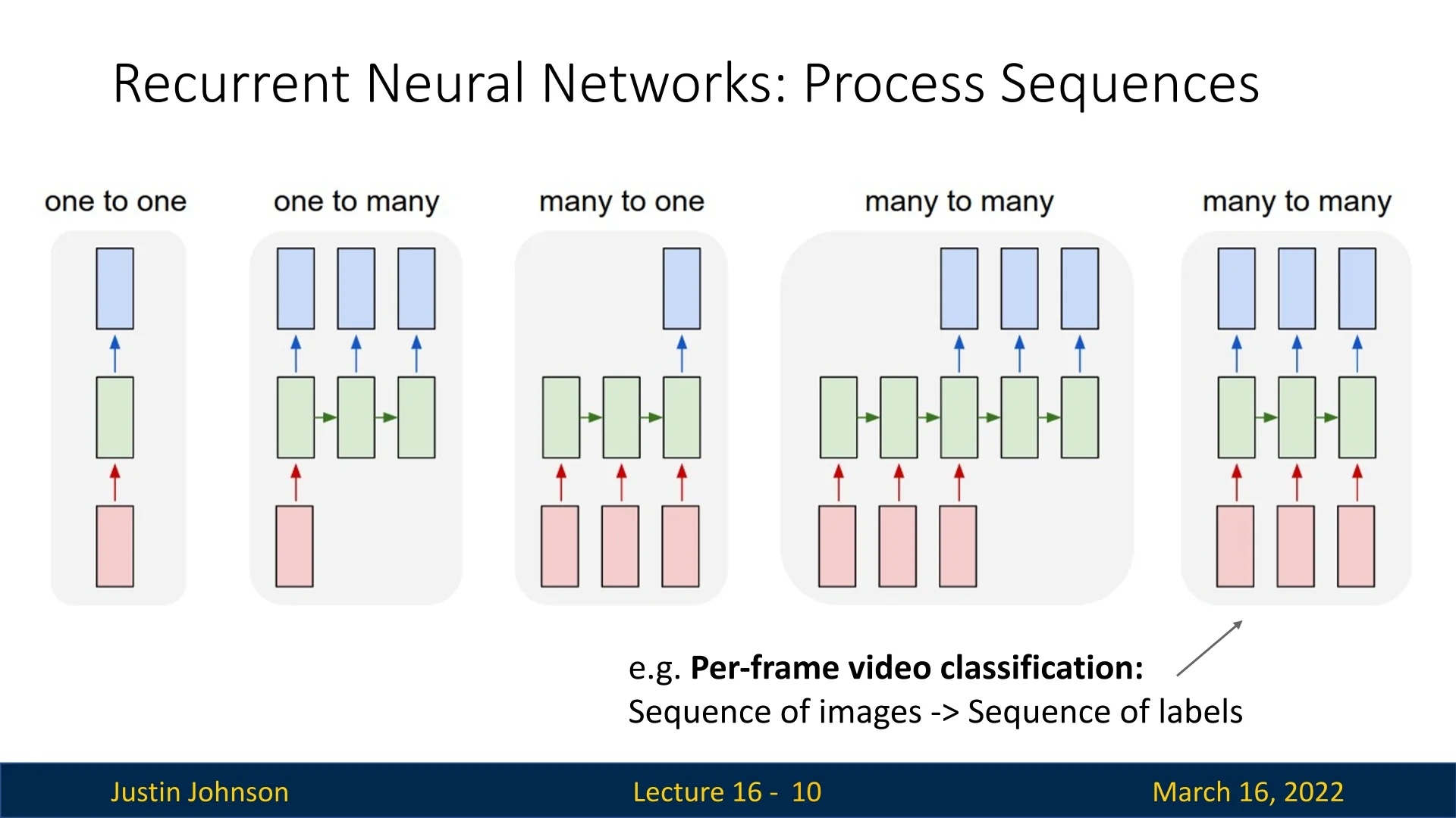
Sequential modeling is crucial for various applications where past observations influence future predictions. Without specialized architectures, we cannot effectively solve tasks such as:
- Image Captioning (One-to-Many): Generating a sequence of words to describe an image requires understanding both spatial and sequential dependencies [669].
- Video Classification (Many-to-One): Classifying an action or event in a video requires processing frames as a sequence, capturing motion and context [288].
- Machine Translation (Many-to-Many): Translating sentences from one language to another requires modeling sequential dependencies across different languages [616].
- Time-Series Forecasting: Financial market predictions, weather forecasting, and power grid monitoring depend on capturing trends and long-term dependencies.
- Sequence Labeling: Named entity recognition, part-of-speech tagging, and handwriting recognition require assigning labels to elements of a sequence while maintaining context.
- Autoregressive Generation: Music composition, text generation, and speech synthesis involve generating outputs where each step depends on previous ones.
16.1.2 RNNs as a General-Purpose Sequence Model
Unlike traditional models that require a fixed input size, RNNs provide a unified architecture for handling sequences of arbitrary length. This flexibility allows RNNs to process short and long sequences using the same model, making them suitable for tasks ranging from speech processing to video analysis.
Although RNNs are designed for sequential data, they can also be applied to non-sequential tasks by processing an input sequentially. For instance, instead of analyzing an image in a single forward pass, an RNN can take a series of glimpses and make a decision based on accumulated information.
16.1.3 RNNs for Visual Attention and Image Generation
Recurrent Neural Networks are traditionally used for sequence modeling, but they can also be leveraged to process images in a sequential manner. Two notable applications include:
- Visual Attention Mechanisms: Instead of processing an entire image at once, an RNN can take a series of glimpses, deciding where to focus next based on previous observations.
- Autoregressive Image Generation: Instead of generating an image in one step, an RNN can incrementally refine an output, painting it sequentially over time.
Visual Attention: Sequential Image Processing
A compelling use case of RNNs in non-sequential tasks is visual attention, where an RNN dynamically determines where to focus within an image. This approach is exemplified by [20], which uses an RNN to sequentially analyze different parts of an image before making a classification decision.
- At each timestep, the network decides which region of the image to examine based on all previously acquired information.
- This process continues over multiple timesteps, accumulating evidence before making a final classification decision.
- A practical example is using RNNs for MNIST digit classification, where instead of viewing the full image at once, the network sequentially attends to different regions before determining the digit.
Autoregressive Image Generation with RNNs
Another fascinating application of RNNs is in image generation, as demonstrated by [193]. Instead of generating an entire image in one step, the model incrementally constructs it over multiple timesteps:
- The model ”draws” small portions of the image sequentially, refining details at each step.
- At each timestep, the RNN decides where to modify the canvas and what details to add.
- This mimics the human drawing process, where an artist sequentially sketches and refines different parts of an image.
The DRAW model [193] exemplifies this approach, using recurrent layers to iteratively generate and improve an image.
These examples illustrate that RNNs are not limited to temporal sequences—they can also be used in spatially structured tasks by treating an image as a sequence of observations or drawing steps.
16.1.4 Limitations of Traditional Neural Networks for Sequential Data
The inability of FC networks and CNNs to capture temporal dependencies leads to major limitations when dealing with sequential tasks. The following table highlights the key differences:
| Characteristic | FC Networks | CNNs | RNNs |
|---|---|---|---|
| Handles Sequential Data | No | No | Yes |
| Shares Parameters Across Time | No | No | Yes |
| Captures Long-Term Dependencies | No | No | Partially (with LSTMs/GRUs) |
| Suitable for Variable-Length Input | No | Partially (1D CNNs) | Yes |
16.1.5 Overview of Recurrent Neural Networks (RNNs) and Their Evolution
Many tasks in modern machine learning involve sequential or time-dependent data, where the observation at time \(t\) depends on the history of inputs \(x_1,\dots ,x_{t-1}\). Classical feedforward networks (fully connected or convolutional) typically assume that inputs are independent and identically distributed (i.i.d.), so they struggle to model such temporal dependencies. Recurrent Neural Networks (RNNs) address this limitation by introducing a hidden state that is passed from one timestep to the next, allowing the model to accumulate information over sequences of (in principle) arbitrary length.
Enrichment 16.1.5.1: How to read this overview
This subsection is intentionally a high-level roadmap of sequence modeling architectures, from basic recurrence to modern attention-based models. Our goal here is to explain why each step in this evolution was introduced and how it addresses the limitations of the previous step. We only sketch the core ideas and equations; rigorous derivations (including Backpropagation Through Time, gating equations, and attention mechanisms), implementation details, and additional examples will follow in dedicated subsections later in this chapter and in the subsequent chapter on Transformers.
RNN progression: from vanilla units to gated architectures
Vanilla RNNs: the basic recurrent idea The simplest recurrent architecture, often called an Elman RNN, maintains a hidden state \(\mathbf {h}_t\) that is updated at each timestep \(t\) via
\begin {equation} \mathbf {h}_t = \tanh \Bigl ( \mathbf {W}_{hh}\,\mathbf {h}_{t-1} + \mathbf {W}_{xh}\,\mathbf {x}_t + \mathbf {b} \Bigr ), \label {eq:chapter16_vanilla_rnn_recurrence} \end {equation}
where \(\mathbf {x}_t\) is the input at time \(t\), \(\mathbf {h}_t\) is the hidden state, and the same parameters \(\mathbf {W}_{hh}\), \(\mathbf {W}_{xh}\), and \(\mathbf {b}\) are reused for all timesteps. This weight sharing is what gives RNNs their ability to generalize across sequence length.
However, as we will see in detail when we derive Backpropagation Through Time (BPTT), repeatedly multiplying by \(\mathbf {W}_{hh}\) causes gradients to either shrink to zero or explode in magnitude over long sequences. This is the classical vanishing/exploding gradient problem [35, 485]. In practice:
- Gradients often vanish, making it hard for vanilla RNNs to learn dependencies beyond roughly 10–50 timesteps.
- Gradients can also explode when \(\|\mathbf {W}_{hh}\|\) is too large or activations allow unbounded growth, which is typically mitigated with gradient clipping.
Later in this chapter we will revisit Vanilla RNN and formally analyze why these issues arise and how techniques such as truncated BPTT partially alleviate them.
LSTMs: gating and additive memory for long-term dependencies To handle much longer temporal dependencies (hundreds of steps), Long Short-Term Memory (LSTM) networks [236] modify the recurrence in two crucial ways:
- 1.
- They maintain a separate cell state that is updated additively, creating a path where information and gradients can flow over many timesteps with minimal attenuation.
- 2.
- They introduce gates (input, forget, and output) that learn when to write new information to the cell state, when to erase old information, and when to expose the cell state to the hidden state.
Intuitively, the LSTM turns the hidden dynamics into a differentiable memory system that can learn to “remember” and “forget” over long horizons. This largely solves the vanishing gradient problem for many practical sequence lengths and made LSTMs the dominant architecture for years in speech recognition, language modeling, and other temporal tasks. The trade-off is increased complexity: each LSTM cell contains several interacting affine transformations and gates, increasing parameter count and compute cost relative to vanilla RNNs.
GRUs: simplifying the LSTM while keeping most benefits Gated Recurrent Units (GRUs) [107] were proposed as a streamlined alternative to LSTMs. GRUs merge the LSTM’s input and forget gates into a single update gate and remove the explicit cell state, directly updating the hidden state instead. This yields:
- Fewer parameters and simpler computation compared to LSTMs.
- Empirically similar performance to LSTMs on many language and sequence modeling benchmarks, especially for moderate sequence lengths.
From an evolutionary perspective, GRUs are motivated by a design question: how much of the LSTM’s complexity is truly necessary to combat vanishing gradients? GRUs show that a simpler gating mechanism can capture much of the benefit, which is attractive in resource-limited or latency-sensitive settings.
Bidirectional RNNs: using both past and future Vanilla RNNs, LSTMs, and GRUs as defined above are causal: at time \(t\), the model only has access to the past and current inputs \((x_1,\dots ,x_t)\). For many applications, however, the entire sequence is available at once. Bidirectional RNNs address this by running one RNN forward in time and another backward, then combining their hidden states (e.g., by concatenation) at each timestep.
This evolution is motivated by disambiguation through context: for the token “bank” in the sentence “He went to the bank to fish”, a backward RNN that sees “to fish” can help decide that “bank” refers to the side of a river rather than a financial institution. Bidirectional RNNs therefore excel in tasks like text classification, named entity recognition, and offline speech transcription, but they are not suitable for real-time streaming applications where future inputs are not yet observed.
Motivation toward Transformers and attention-based models
The sequential bottleneck and fixed-size state Despite the success of LSTMs, GRUs, and bidirectional variants, all RNN-based models share two structural limitations:
- 1.
- Sequential computation across time: To compute \(\mathbf {h}_t\), we must first compute \(\mathbf {h}_{t-1}\). This dependency chain prevents parallelization across timesteps, making training and inference less efficient on modern accelerators for very long sequences.
- 2.
- Fixed-size hidden state: The hidden state \(\mathbf {h}_t\) is a vector of fixed dimension that must compress all past information. For extremely long contexts (thousands of tokens), this global bottleneck can limit the model’s capacity to selectively remember detailed information.
These limitations motivated architectures that could (i) process all positions in a sequence in parallel, and (ii) dynamically allocate capacity by letting each position attend to the most relevant parts of the sequence.
Transformers: replacing recurrence with self-attention The Transformer architecture [664] removes recurrence altogether and instead uses self-attention layers: each token computes weighted combinations of all other tokens in the sequence. At a high level:
- All timesteps can be processed in parallel within a layer, dramatically improving training efficiency on GPUs and TPUs.
- Long-range dependencies are handled naturally, since attention weights can connect arbitrarily distant positions without repeatedly multiplying by a transition matrix.
However, this shift introduces new trade-offs:
- The memory and compute cost of self-attention scales quadratically as \(O(T^2)\) with sequence length \(T\), which becomes challenging for very long inputs.
- For autoregressive generation (e.g., language modeling), outputs are still typically produced token by token, and each new token requires computing attention over the growing context. This can be slow for extremely long outputs, although techniques such as speculative decoding [748] and non-autoregressive models [198] aim to alleviate this by partially parallelizing generation or reducing the number of decoding steps.
Later, when we discuss attention mechanisms in depth, we will connect these design decisions back to the limitations of RNNs described above.
Roadmap for the rest of the chapter
The remainder of this chapter builds on this evolutionary story and revisits each model family in more depth:
- 1.
- Vanilla RNNs and BPTT: We begin by formalizing vanilla RNNs, deriving Backpropagation Through Time, and precisely characterizing why and when vanishing and exploding gradients occur.
- 2.
- LSTMs and GRUs: We then introduce LSTMs and GRUs from first principles, writing out their gating equations and explaining how additive memory paths and learned gates mitigate vanishing gradients, along with their remaining limitations (sequential computation, fixed-size state).
- 3.
- Beyond RNNs: Finally, we use the insights from gated RNNs to motivate attention-based architectures and Transformers, which replace recurrent hidden states with self-attention, enabling highly parallel training and more flexible modeling of long-range dependencies. Detailed coverage of Transformer variants and attention mechanisms appears in the following chapter.
By first presenting this high-level overview and then returning to each model class in detail, we aim to make the connections between architectures explicit: each new design (gating, bidirectionality, attention) can be understood as an attempt to systematically overcome the optimization and representation bottlenecks of its predecessors.
16.2 Recurrent Neural Networks (RNNs) - How They Work
Recurrent Neural Networks (RNNs) process sequential data by maintaining an internal state that evolves over time. Unlike feedforward neural networks that process inputs independently, RNNs retain memory through recurrent connections, enabling them to model dependencies across time steps.
At each timestep \( t \), a new input \( x_t \) is provided to the RNN. The network updates its hidden state \( h_t \) based on both the current input and the previous hidden state \( h_{t-1} \), producing an output \( y_t \): \[ h_t = f_W(h_{t-1}, x_t), \] where \( f_W \) is the recurrence function, typically a non-linear function such as \(\tanh \). A key property of RNNs is that the same function and parameters are used at every time step. The weights \( W \) are shared across all time steps, allowing the model to process sequences of arbitrary length.
Expanding this, a simple or ”vanilla” RNN is formally defined as: \[ h_t = \tanh (W_{hh}h_{t-1} + W_{xh}x_t + b), \] \[ y_t = W_{hy}h_t. \] This architecture, sometimes called a vanilla RNN or Elman RNN after Prof. Jeffrey Elman, efficiently processes sequences by applying the same weight matrices repeatedly. Note: we’ll often omit the bias from the notation for simplicity, but don’t forget it when you implement RNNs.
16.2.1 RNN Computational Graph
Since RNNs process sequences iteratively, we can represent their computation graph by unrolling the network over time. The computational graph depends on how inputs and outputs are structured, leading to different sequence processing scenarios.
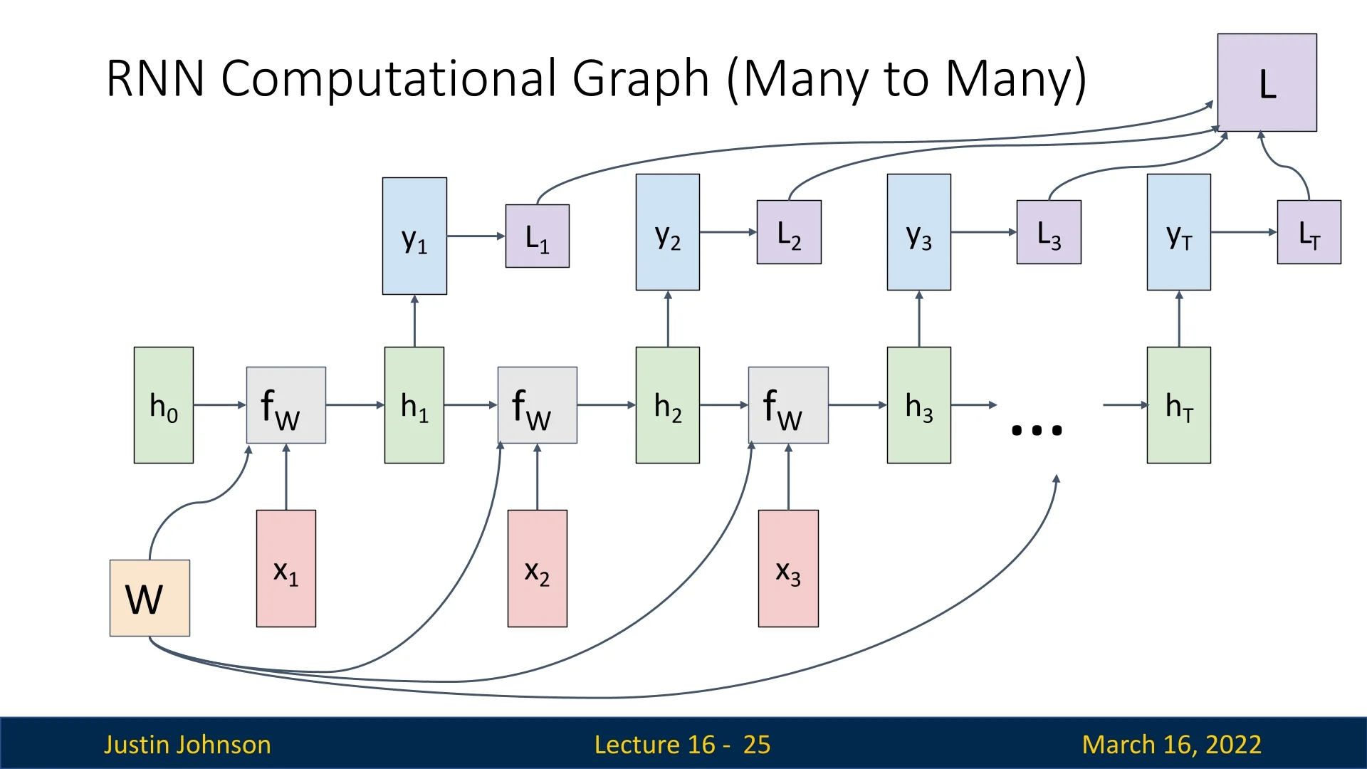
Many-to-Many
In a many-to-many setup, an RNN processes a sequence of inputs and generates a sequence of outputs. Each hidden state depends on the previous state and the current input: \[ h_t = f_W(h_{t-1}, x_t), \quad y_t = W_{hy}h_t. \]
The initial hidden state \( h_0 \) is typically initialized as a zero vector or sampled from a normal distribution. However, in some architectures, \( h_0 \) is treated as a learnable parameter, allowing it to be optimized during training. This can be beneficial when early time steps contain little useful information.
The network processes each input sequentially:
- \( x_1 \) is combined with \( h_0 \) using \( f_W \), producing \( h_1 \) and output \( y_1 \).
- \( h_1 \) is used with \( x_2 \) to compute \( h_2 \), which generates \( y_2 \).
- This process repeats until reaching the final time step \( T \).
Since the same weight matrix is reused at every time step, the computational graph is unrolled for as long as the sequence continues. During backpropagation, gradients must be summed across all timesteps (As we use the same node in multiple parts of the computation graph).
Training an RNN involves applying a loss function at each timestep: \[ L = \sum _{t=1}^{T} L_t, \] where \( L_t \) is the loss at time \( t \). The summed loss is then used for backpropagation.
Many-to-One
Some tasks require processing a sequence of inputs but generating only a single output at the final time step. This many-to-one setting is common in applications such as video classification, where the entire sequence is used to predict one label.
Instead of computing outputs at each timestep, the RNN produces a final output at step \( T \), based on the last hidden state \( h_T \): \[ y = W_{hy}h_T. \] The loss function is then computed using only the final output \( y_T \), such as cross-entropy (CE) loss for classification.
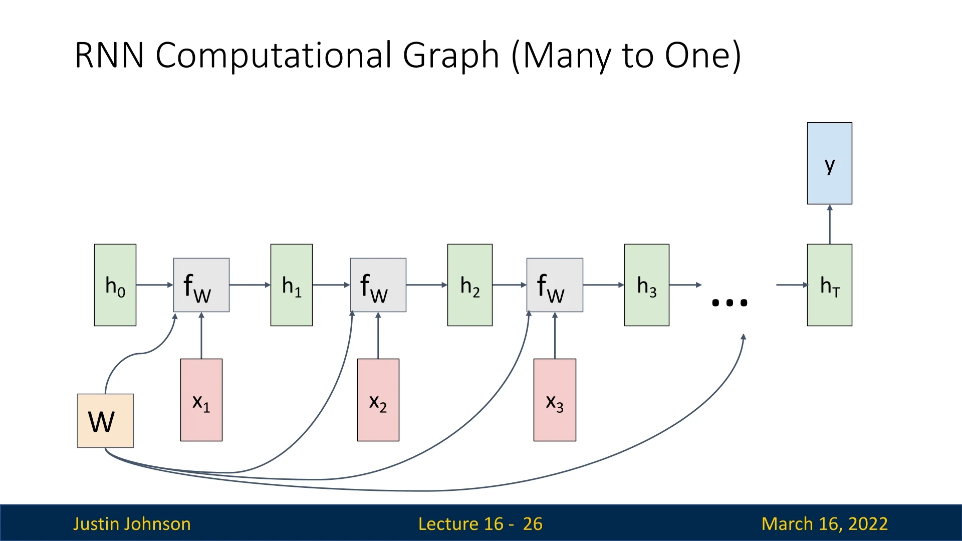
This structure is particularly useful when the full context of the sequence is needed to make an informed decision, such as recognizing an action from a video or predicting sentiment from a passage of text.
One-to-Many
In contrast, one-to-many architectures take a single input and generate a sequence of outputs. This is commonly used in generative tasks such as image captioning, where the network produces a sequence of words based on an input image.
The RNN is initialized with an input \( x \) and generates outputs iteratively: \[ h_1 = f_W(h_0, x), \quad y_1 = W_{hy}h_1. \] The output \( y_1 \) is then fed as input at the next timestep: \[ h_2 = f_W(h_1, y_1), \quad y_2 = W_{hy}h_2. \]
The sequence continues until a special END token is produced, signaling termination.
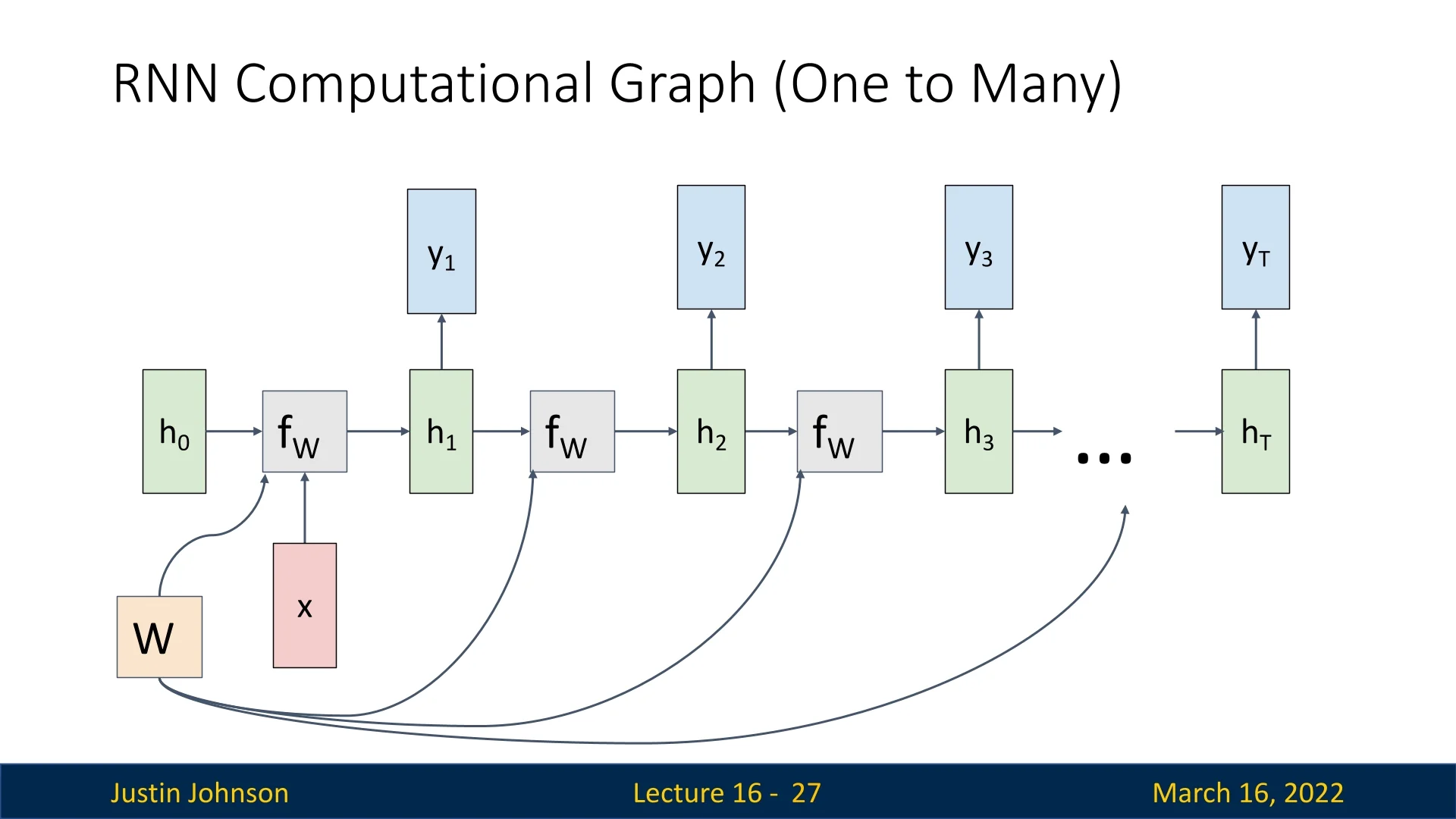
The network must learn to balance sequential coherence while ensuring that the generated sequence remains contextually relevant.
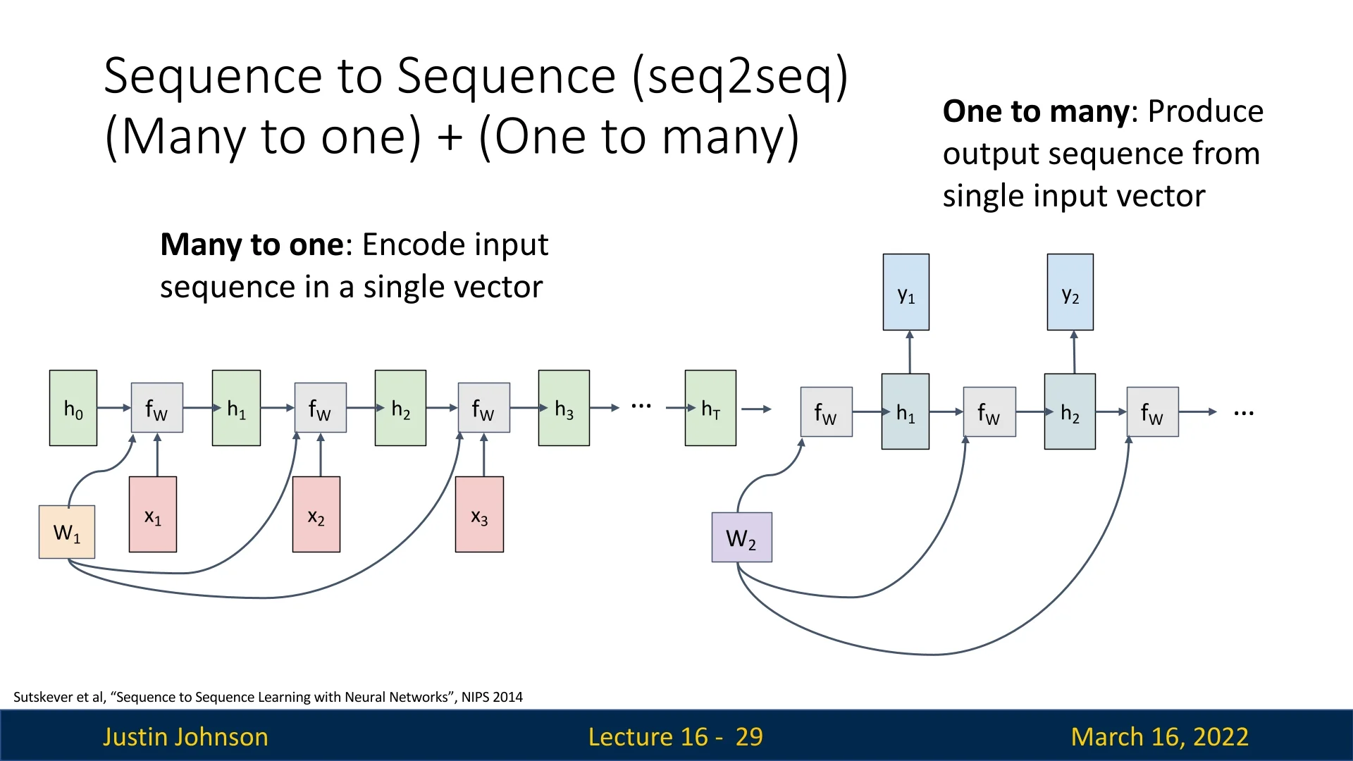
16.2.2 Seq2Seq: Sequence-to-Sequence Learning
Many real-world problems involve mapping an input sequence to an output sequence where the lengths can differ arbitrarily (\(T \neq M\)). A canonical example is machine translation, where an input sentence in one language (e.g. English) is converted into a sentence in another language (e.g. French); the two sentences may have different lengths and word orders.
To handle this setting, Sequence-to-Sequence (Seq2Seq) models [616] use a composite architecture consisting of two Recurrent Neural Networks with separate parameters:
- Encoder (many-to-one). Uses weights \(W_1\) to read the input sequence and compress it into a single vector.
- Decoder (one-to-many). Uses weights \(W_2\) to expand this single vector into an output sequence.
In Justin Johnson’s slides (see the below figure), this is summarized as \[ \mbox{Seq2Seq} = (\mbox{many-to-one}) + (\mbox{one-to-many}). \]
The encoder–decoder architecture
Let the input sequence be \(\mathbf {x} = (x_1,\dots ,x_T)\) and the output sequence be \(\mathbf {y} = (y_1,\dots ,y_M)\).
- 1.
- Encoder (many-to-one, weights \(W_1\)). The encoder RNN processes the input sequence step by step: \begin {equation} h^{\mbox{enc}}_t = f_W\!\bigl (h^{\mbox{enc}}_{t-1}, x_t; W_1\bigr ), \qquad t = 1,\dots ,T, \label {eq:chapter16_seq2seq_encoder} \end {equation} where \(f_W\) denotes the recurrent update (RNN, LSTM, GRU, etc.) and \(h^{\mbox{enc}}_0\) is typically initialized to the zero vector. The final encoder state \begin {equation} h^{\mbox{enc}}_T \end {equation} serves as a fixed-size context vector summarizing the entire input sequence. In the figure, these encoder states are drawn as \(h_0, h_1, \dots , h_T\).
- 2.
- Information transfer (many-to-one \(\to \) one-to-many). The decoder is initialized from the encoder’s final state: \begin {equation} h^{\mbox{dec}}_0 = h^{\mbox{enc}}_T, \label {eq:chapter16_seq2seq_handover} \end {equation} which corresponds to the arrow from \(h_T\) into the first decoder cell in the below figure. This vector \(h^{\mbox{enc}}_T\) is the single “input” to the decoder side.
- 3.
- Decoder (one-to-many, weights \(W_2\)). Starting from \(h^{\mbox{dec}}_0\) and a special <START> token \(y_0\), the decoder generates the output sequence autoregressively using its own parameters \(W_2\): \begin {equation} h^{\mbox{dec}}_t = f_W\!\bigl (h^{\mbox{dec}}_{t-1}, y_{t-1}; W_2\bigr ), \qquad t = 1,\dots ,M, \label {eq:chapter16_seq2seq_decoder_state} \end {equation} \begin {equation} p(y_t \mid y_{<t}, \mathbf {x}) = \mathrm {softmax}\bigl (W_{\mbox{out}} h^{\mbox{dec}}_t\bigr ), \label {eq:chapter16_seq2seq_decoder_output} \end {equation} where \(W_{\mbox{out}}\) maps hidden states to vocabulary logits. During training, we typically use teacher forcing, feeding the ground-truth token \(y_{t-1}\) into (16.5); at inference time, \(y_{t-1}\) is the token predicted at the previous step (e.g. \(\arg \max \) of (16.6)). In the figure, the decoder hidden states \(h^{\mbox{dec}}_1, h^{\mbox{dec}}_2,\dots \) are drawn as \(h_1, h_2,\dots \), each producing outputs \(y_1, y_2,\dots \).
Decoding continues until the model emits a special <END> token, indicating that the output sequence is complete. In this way, a single encoded vector \(h^{\mbox{enc}}_T\) is “unrolled” into an output of arbitrary length \(M\).
Significance and the information bottleneck
Seq2Seq models extend RNNs from fixed-size input/output settings to a general framework for transforming one sequence into another, enabling applications such as:
- Machine translation: Converting text between languages (e.g. English \(\to \) French).
- Speech recognition: Mapping acoustic feature sequences to text.
- Text summarization: Compressing long documents into shorter summaries.
- Conversational AI: Generating responses in dialog systems.
At the same time, the basic encoder–decoder design introduces a fundamental information bottleneck:
- All information about the input sequence \(\mathbf {x}\) must be packed into the single vector \(h^{\mbox{enc}}_T\) in (16.4).
- For long inputs, early tokens \((x_1, x_2, \dots )\) may have only a weak influence on \(h^{\mbox{enc}}_T\) due to vanishing gradients and limited capacity, leading to degraded translation or generation quality.
This limitation motivates several extensions that we will develop later in the chapter and in subsequent chapters:
- Gated recurrent units (LSTMs, GRUs) improve how information and gradients propagate through time, making the context vector \(h^{\mbox{enc}}_T\) more robust for longer sequences.
- Attention mechanisms allow the decoder to look back at all encoder states \((h^{\mbox{enc}}_1,\dots ,h^{\mbox{enc}}_T)\) instead of relying solely on \(h^{\mbox{enc}}_T\), thereby softening the bottleneck.
In the next parts, we will connect this generic Seq2Seq template to concrete tasks such as language modeling, derive Backpropagation Through Time (BPTT) for training these models, and then revisit the roles of LSTMs, GRUs, and attention in improving sequence-to-sequence learning.
16.3 Example Usage of Seq2Seq: Language Modeling
A concrete example of how recurrent networks operate in practice is a character-level language model. The goal is to process a stream of input characters and, at each timestep, predict the next character in the sequence. By learning the conditional distribution \[ p(x_t \mid x_1,\dots ,x_{t-1}), \] the model captures the statistical structure of the training text and can later be used to generate new text.
16.3.1 Formulating the problem
Consider the toy training sequence “hello” with vocabulary \[ \mathcal {V} = \{\mbox{h}, \mbox{e}, \mbox{l}, \mbox{o}\}. \] We view this as a supervised learning problem where, at each timestep, the input is the current character and the target is the next character:
| t | Input | Target |
| 1 | “h” | “e” |
| 2 | “e” | “l” |
| 3 | “l” | “l” |
| 4 | “l” | “o” |
Each character is represented as a one-hot vector in \(\mathbb {R}^{|\mathcal {V}|}\), for example: \[ \mathbf {x}_{\mbox{h}} = [1\;0\;0\;0]^\top ,\quad \mathbf {x}_{\mbox{e}} = [0\;1\;0\;0]^\top ,\quad \mathbf {x}_{\mbox{l}} = [0\;0\;1\;0]^\top ,\quad \mathbf {x}_{\mbox{o}} = [0\;0\;0\;1]^\top . \]
16.3.2 Forward pass through time
A simple RNN with hidden state dimension \(H\) maintains a hidden vector \(\mathbf {h}_t \in \mathbb {R}^H\) and updates it according to \[ \mathbf {h}_t = \tanh \!\bigl (\mathbf {W}_{hh}\mathbf {h}_{t-1} + \mathbf {W}_{xh}\mathbf {x}_t + \mathbf {b}_h\bigr ), \] where \(\mathbf {h}_0\) is an initial state (often the zero vector), \(\mathbf {W}_{xh}\) maps inputs to the hidden layer, \(\mathbf {W}_{hh}\) maps the previous hidden state to the new one, and \(\mathbf {b}_h\) is a bias term shared across time.
From the hidden state, the network produces unnormalized scores (logits) over the next character: \[ \mathbf {y}_t = \mathbf {W}_{hy}\mathbf {h}_t + \mathbf {b}_y, \] with \(\mathbf {W}_{hy}\) and \(\mathbf {b}_y\) shared at all timesteps. Applying a softmax gives a probability distribution over the vocabulary: \[ \mathbf {p}_t = \mathrm {softmax}(\mathbf {y}_t), \qquad (\mathbf {p}_t)_k = \frac {\exp ((\mathbf {y}_t)_k)}{\sum _{j}\exp ((\mathbf {y}_t)_j)}. \]
For example, for the first character “h”, we feed \(\mathbf {x}_1 = \mathbf {x}_{\mbox{h}}\) into the RNN to obtain a hidden state and logits: \[ \mathbf {h}_1 = [0.3,\,-0.1,\,0.9]^\top ,\qquad \mathbf {y}_1 = [1.0,\,2.2,\,-3.0,\,4.1]^\top , \] so that \(\mathbf {p}_1 = \mathrm {softmax}(\mathbf {y}_1)\) assigns high probability to the correct next character “e”. The same computation is repeated for “e”, “l”, and “l”, with the hidden state carrying information about the context seen so far (“h”, “he”, “hel”, “hell”).
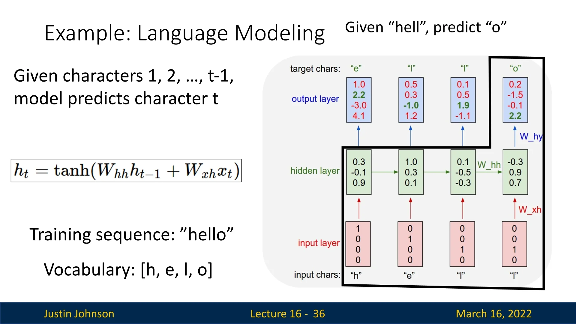
Figure 16.6 illustrates this process: given characters up to time \(t-1\) (for example, “he”), the model predicts character \(t\) (“l”); then the new hidden state is forwarded to the next timestep.
16.3.3 Training: losses and gradient flow through time
To train the model, we compare its predictions with the ground-truth next characters and update the shared weights \[ \Theta = \{\mathbf {W}_{xh}, \mathbf {W}_{hh}, \mathbf {W}_{hy}, \mathbf {b}_h, \mathbf {b}_y\}. \]
Per-timestep loss
At each timestep \(t\), the target next character \(x_{t+1}\) is represented as a one-hot vector \(\mathbf {t}_{t+1} \in \mathbb {R}^{|\mathcal {V}|}\). We compute the cross-entropy loss between \(\mathbf {p}_t\) and \(\mathbf {t}_{t+1}\): \[ L_t = - \sum _{k=1}^{|\mathcal {V}|} (\mathbf {t}_{t+1})_k \log (\mathbf {p}_t)_k = - \log (\mathbf {p}_t)_{k^\star }, \] where \(k^\star \) is the index of the true next character at time \(t+1\). For the sequence “hello” we obtain losses \(L_1,\dots ,L_4\) corresponding to the four training pairs listed above.
Sequence loss and gradient
The total loss for the sequence is the sum of per-timestep losses: \[ \mathcal {L} = \sum _{t=1}^{T} L_t. \] Because the same parameters \(\Theta \) are reused at every timestep, the gradient of the sequence loss with respect to any parameter (for example, \(\mathbf {W}_{hh}\)) is the sum of its contributions from each timestep: \[ \frac {\partial \mathcal {L}}{\partial \mathbf {W}_{hh}} = \sum _{t=1}^{T} \frac {\partial L_t}{\partial \mathbf {W}_{hh}}. \]
Each term \(\partial L_t / \partial \mathbf {W}_{hh}\) is itself a chain of derivatives that passes backward through time. For instance, the loss \(L_4\) (predicting “o” given the prefix “hell”) depends on \(\mathbf {h}_4\), which depends on \(\mathbf {h}_3\), which depends on \(\mathbf {h}_2\), and so on back to \(\mathbf {h}_0\). Computing the gradient therefore requires propagating error signals through the entire sequence of hidden states: \[ \mathbf {h}_4 \rightarrow \mathbf {h}_3 \rightarrow \mathbf {h}_2 \rightarrow \mathbf {h}_1 \rightarrow \mathbf {h}_0. \]
Once the gradient \(\nabla _{\Theta } \mathcal {L}\) has been computed, we update the parameters using gradient descent or a variant such as Adam: \[ \Theta \leftarrow \Theta - \eta \,\nabla _{\Theta } \mathcal {L}, \] where \(\eta \) is the learning rate and the negative gradient gives the direction of steepest decrease of the loss.
The procedure for computing these gradients by explicitly following the chain of dependencies backward in time is called Backpropagation Through Time (BPTT). In the next section, we will make this precise by unrolling the RNN across timesteps and deriving the gradient expressions. This will naturally expose numerical issues such as vanishing and exploding gradients when sequences become long.
16.3.4 Inference: generating text
After training, we can use the model to generate new text, one character at a time:
- 1.
- Initialize the hidden state \(\mathbf {h}_0\) (e.g. zeros) and feed an initial character or a special <START> symbol \(\mathbf {x}_1\).
- 2.
- Compute \(\mathbf {h}_1\), logits \(\mathbf {y}_1\), and probabilities \(\mathbf {p}_1 = \mathrm {softmax}(\mathbf {y}_1)\).
- 3.
- Sample or choose the most likely next character from \(\mathbf {p}_1\) (e.g. by \(\arg \max \)), obtaining a character \(x_2\).
- 4.
- Feed the one-hot encoding of \(x_2\) back in as the next input \(\mathbf {x}_2\) and repeat.
This autoregressive loop continues until the model produces a special <END> token or a maximum length is reached.
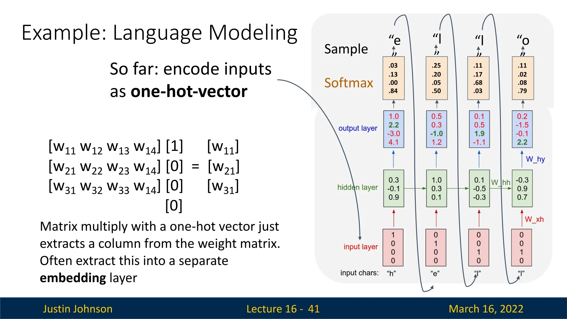
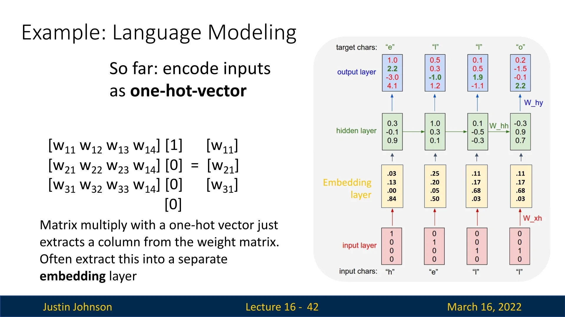
16.3.5 From one-hot vectors to embeddings
So far we have used one-hot vectors as inputs. Multiplying a weight matrix \(\mathbf {W}_{xh}\) by a one-hot vector simply selects one column of \(\mathbf {W}_{xh}\), which can be interpreted as a learned embedding of that character. Modern implementations therefore introduce an explicit embedding layer that maps character indices to dense vectors: \[ \mathbf {e}_t = \mathrm {Embedding}(x_t), \qquad \mathbf {h}_t = \tanh \!\bigl (\mathbf {W}_{hh}\mathbf {h}_{t-1} + \mathbf {W}_{eh}\mathbf {e}_t + \mathbf {b}_h\bigr ), \] where \(\mathbf {W}_{eh}\) plays the role of \(\mathbf {W}_{xh}\) but acts on lower-dimensional embeddings.
This has several advantages:
- Efficiency. We avoid explicitly storing and multiplying large sparse one-hot vectors; indexing into an embedding table is cheaper.
- Learned similarity structure. Characters (or words) with similar usage patterns can acquire similar embedding vectors, helping the model generalize.
- Flexible dimensionality. The embedding dimension can be chosen independently of the vocabulary size, controlling the capacity and computational cost.
16.3.6 Summary and motivation for BPTT
In this example, we have seen how an RNN processes a character sequence like “hello”, predicts the next character at each timestep, aggregates per-timestep cross-entropy losses into a sequence loss, and uses gradients of this loss to update a set of shared parameters. The key difficulty is that the loss at later timesteps depends on a long chain of hidden states and repeated applications of the same weight matrices. Computing and propagating gradients through this temporal chain is precisely the job of Backpropagation Through Time. In the next section we will unroll the RNN formally, derive these gradients, and use that derivation to understand why naïve RNNs suffer from vanishing and exploding gradients on long sequences.
16.4 Backpropagation Through Time (BPTT)
In a Recurrent Neural Network (RNN), the hidden state at time \(t\) depends on the hidden state at time \(t-1\), so unrolling the network over a sequence of length \(T\) yields a deep computational graph with \(T\) repeated applications of the same parameters. Training therefore requires computing gradients not only “through layers” (as in feedforward networks) but also through time. This procedure is known as Backpropagation Through Time (BPTT).
16.4.1 Full BPTT as Backprop on an Unrolled RNN
Consider a simple (vanilla) RNN processing a sequence of length \(T\) with inputs \(\mathbf {x}_1, \dots , \mathbf {x}_T\). The forward dynamics are \begin {align} \mathbf {h}_t &= \phi \!\bigl (\mathbf {W}_{hh}\mathbf {h}_{t-1} + \mathbf {W}_{xh}\mathbf {x}_t + \mathbf {b}_h\bigr ), \qquad t = 1,\dots ,T, \label {eq:chapter16_rnn_forward_h}\\ \mathbf {y}_t &= \mathbf {W}_{hy}\mathbf {h}_t + \mathbf {b}_y, \label {eq:chapter16_rnn_forward_y} \end {align}
where \(\mathbf {h}_0\) is an initial hidden state (often the zero vector or a learned parameter), \(\phi \) is a pointwise activation function (typically \(\tanh \) in classical RNNs), and \(\mathbf {W}_{xh}, \mathbf {W}_{hh}, \mathbf {W}_{hy}, \mathbf {b}_h, \mathbf {b}_y\) are shared across all timesteps.
Let \(\mathcal {L}_t = \ell (\mathbf {y}_t, \mathbf {y}_t^{\mbox{target}})\) denote the loss at timestep \(t\), and define the total sequence loss \[ \mathcal {L} = \sum _{t=1}^{T} \mathcal {L}_t. \] Because parameters are shared in time, the gradient of the total loss with respect to any parameter \(\theta \in \{\mathbf {W}_{xh}, \mathbf {W}_{hh}, \mathbf {W}_{hy}, \mathbf {b}_h, \mathbf {b}_y\}\) decomposes as \[ \frac {\partial \mathcal {L}}{\partial \theta } = \sum _{t=1}^{T} \frac {\partial \mathcal {L}_t}{\partial \theta }. \]
The key difficulty is that \(\mathcal {L}_t\) depends on \(\theta \) not only through the “local” timestep \(t\), but also through the entire history of hidden states \(\mathbf {h}_1,\dots ,\mathbf {h}_t\). For example, for the recurrent weight matrix \(\mathbf {W}_{hh}\) we can write \begin {equation} \frac {\partial \mathcal {L}_t}{\partial \mathbf {W}_{hh}} = \sum _{k=1}^{t} \underbrace {\frac {\partial \mathcal {L}_t}{\partial \mathbf {h}_t}}_{\mbox{error at time }t} \;\underbrace {\frac {\partial \mathbf {h}_t}{\partial \mathbf {h}_k}}_{\mbox{temporal Jacobian }k \rightarrow t} \;\underbrace {\frac {\partial ^+ \mathbf {h}_k}{\partial \mathbf {W}_{hh}}}_{\mbox{local derivative at time }k}, \label {eq:chapter16_bptt_chain} \end {equation} where \(\partial ^+ \mathbf {h}_k / \partial \mathbf {W}_{hh}\) treats \(\mathbf {h}_{k-1}\) as constant.
The temporal Jacobian \(\partial \mathbf {h}_t / \partial \mathbf {h}_k\) itself is a product of one-step Jacobians: \begin {equation} \frac {\partial \mathbf {h}_t}{\partial \mathbf {h}_k} = \prod _{j=k+1}^{t} \frac {\partial \mathbf {h}_j}{\partial \mathbf {h}_{j-1}}, \qquad \frac {\partial \mathbf {h}_j}{\partial \mathbf {h}_{j-1}} = \mathrm {diag}\!\bigl (\phi '(\mathbf {z}_j)\bigr )\,\mathbf {W}_{hh}, \label {eq:chapter16_bptt_jacobian_product} \end {equation} where \(\mathbf {z}_j = \mathbf {W}_{hh}\mathbf {h}_{j-1} + \mathbf {W}_{xh}\mathbf {x}_j + \mathbf {b}_h\) are the pre-activations. Thus, BPTT is standard backpropagation applied to the unrolled computational graph, but its gradients involve products of many Jacobian matrices across time.
Vanishing and Exploding Gradients Revisited
Equation (16.8) is the mathematical origin of the two classic pathologies in RNN training [35, 485]. If we denote the one-step Jacobian at time \(j\) by \[ \mathbf {J}_j = \frac {\partial \mathbf {h}_j}{\partial \mathbf {h}_{j-1}} = \mathrm {diag}\!\bigl (\phi '(\mathbf {z}_j)\bigr )\,\mathbf {W}_{hh}, \] then \(\partial \mathbf {h}_t / \partial \mathbf {h}_k = \mathbf {J}_t \mathbf {J}_{t-1} \cdots \mathbf {J}_{k+1}\). On average, the behavior of this product is controlled by typical singular values of \(\mathbf {J}_j\):
- Vanishing gradients. If the largest singular value of a “typical” Jacobian \(\mathbf {J}_j\) is less than \(1\) on average, then \(\bigl \|\partial \mathbf {h}_t / \partial \mathbf {h}_k\bigr \|\) decays approximately like \(\gamma ^{t-k}\) for some effective contraction factor \(0 < \gamma < 1\). Gradients associated with distant timesteps become numerically negligible, making it extremely hard to learn long-range dependencies [35].
- Exploding gradients. If the largest singular value is greater than \(1\) on average, then \(\bigl \|\partial \mathbf {h}_t / \partial \mathbf {h}_k\bigr \|\) grows approximately like \(\gamma ^{t-k}\) with \(\gamma > 1\). Small errors at late timesteps produce enormous gradients for early timesteps, leading to numerical overflow and unstable optimization [485].
These issues arise even if we ignore the nonlinearity and approximate the dynamics as \(\mathbf {h}_t \approx \mathbf {W}_{hh}\mathbf {h}_{t-1}\). In that case, \(\mathbf {h}_t \approx \mathbf {W}_{hh}^t \mathbf {h}_0\), and both the forward states and the backpropagated gradients are governed by powers of the same matrix \(\mathbf {W}_{hh}\). Unless the spectral properties of \(\mathbf {W}_{hh}\) are carefully controlled, either vanishing or exploding behavior is unavoidable.
Memory Cost of Full BPTT
To compute the exact gradients in (16.7), the forward pass must store all hidden states \(\mathbf {h}_1,\dots ,\mathbf {h}_T\) and pre-activations \(\mathbf {z}_1,\dots ,\mathbf {z}_T\), since the Jacobians depend on these values. The activation memory cost therefore scales as \[ \mathcal {O}(T \cdot d_h), \] where \(d_h\) is the hidden dimension. For long sequences (for example, \(T = 1{,}000\) and \(d_h = 1{,}024\)), storing all activations across many layers and mini-batches can easily require gigabytes of memory, even before accounting for optimizer state and other model parameters. Furthermore, each parameter update requires a full forward and backward pass over the entire sequence, which is computationally expensive.
These considerations motivate an approximation that trades exact long-range gradients for tractable memory and compute: truncated BPTT.
16.4.2 Truncated Backpropagation Through Time
In many applications (language modeling, online speech recognition, reinforcement learning), sequences are effectively unbounded: there is no natural “end of sequence” at which we could run full BPTT. Moreover, as we saw in Section 16.4.1.0, the Jacobian products in full BPTT already suffer from vanishing and exploding gradients even for moderate sequence lengths [35, 485]. Truncated BPTT (often denoted TBPTT-\(\tau \)) addresses both the computational and memory costs by limiting the temporal horizon over which gradients are propagated, at the price of introducing additional bias in credit assignment [717].
Chunked Training with a Finite Horizon
Fix a truncation length (or horizon) \(\tau \ll T\), typically in the range \(\tau \approx 50\)–\(200\). We process the sequence in chunks of length \(\tau \) and backpropagate only within each chunk. Concretely, suppose we process a long sequence in segments \([1,\tau ], [\tau +1, 2\tau ], \dots \). For the \(s\)-th chunk we define \[ b_s = (s-1)\tau , \qquad \mbox{chunk } s: \; t = b_s+1, \dots , b_s + \tau . \] The algorithm proceeds as follows [717, 485]:
- 1.
- Initialize the hidden state. For the first chunk, set \(\mathbf {h}_{0}\) to zeros or a learned initial state. For chunk \(s>1\), set the initial state to the final hidden state of the previous chunk: \(\mathbf {h}_{b_s} = \mathbf {h}_{b_{s-1}+\tau }\).
- 2.
- Forward pass over the chunk. For \(t = b_s+1,\dots ,b_s+\tau \), compute \(\mathbf {h}_t\) and \(\mathbf {y}_t\) using ([ref])–([ref]), and accumulate the chunk loss \[ \mathcal {L}^{(s)} = \sum _{t=b_s+1}^{b_s+\tau } \mathcal {L}_t. \]
- 3.
- Backward pass (truncated in time). Backpropagate gradients from \(\mathcal {L}^{(s)}\) only through the timesteps \(b_s+1,\dots ,b_s+\tau \). In practice, we treat \(\mathbf {h}_{b_s}\) as a constant with respect to the parameters (for example, by calling detach in PyTorch), so no gradient flows into the computations that produced \(\mathbf {h}_{b_s}\).
- 4.
- Parameter update. Use the gradients from this chunk to update the parameters \(\theta \). Then move to the next chunk.
From an optimization point of view, the overall objective remains the sum (or average) of per-timestep losses: \[ \mathcal {L} = \sum _{s=1}^{S} \mathcal {L}^{(s)} = \sum _{s=1}^{S}\;\sum _{t=b_s+1}^{b_s+\tau } \mathcal {L}_t, \] where \(S\) is the number of chunks. Some implementations divide by \(S\) (or by \(T\)) to work with an average loss, but the gradient structure is unchanged: each update only uses gradients originating from the most recent \(\tau \) timesteps.
Interaction with Vanishing and Exploding Gradients
Truncated BPTT changes how vanishing and exploding gradients appear, but it does not remove the underlying pathologies analyzed in Section 16.4.1.0. It shortens the dangerous Jacobian products (helping with explosion on very long sequences) while adding a hard cutoff that exacerbates vanishing for long-range dependencies [717, 485].
Exploding gradients: partial mitigation via shorter chains In full BPTT, the gradient from time \(T\) back to time \(1\) involves a product of \(T-1\) Jacobians, \(\prod _{j=1}^{T-1} \mathbf {J}_j\), whose norm typically behaves like \(\|\mathbf {J}\|^{T-1}\) for some average Jacobian norm \(\|\mathbf {J}\|\) [35, 485]. If the dominant singular value of the recurrent Jacobian is slightly larger than \(1\), say \(\|\mathbf {J}\| \approx 1.1\), the gradient can grow as \(1.1^{T}\), leading to catastrophic explosion on long sequences.
Truncated BPTT caps the length of this product at the truncation horizon \(\tau \) [717]: no gradient ever involves more than \(\tau \) Jacobian factors. In the toy example above, the worst-case growth is now \(1.1^{\tau }\) instead of \(1.1^{T}\). For \(T = 1000\) and \(\tau = 50\), this replaces a factor of roughly \(2.5 \times 10^{41}\) by about \(117\), which is much easier to manage with gradient clipping [485].
However, if the per-step Jacobians are highly unstable (for example, \(\|\mathbf {W}_{hh}\| \gg 1\)), gradients can still explode within the \(\tau \)-step window. Empirically and theoretically, truncated BPTT therefore reduces the risk of catastrophic explosion on very long sequences, but does not guarantee stability; gradient clipping remains necessary in practice [485].
Vanishing gradients: soft decay plus hard truncation For vanishing gradients, truncated BPTT actually makes the situation worse for long-range dependencies by combining two effects: the soft exponential decay inherent in vanilla RNNs and an additional hard algorithmic cutoff at the truncation boundary.
Under full BPTT, the gradient of a loss at time \(T\) with respect to an earlier hidden state \(\mathbf {h}_k\) can be written as \[ \frac {\partial \mathcal {L}_T}{\partial \mathbf {h}_k} = \frac {\partial \mathcal {L}_T}{\partial \mathbf {h}_T} \prod _{j=k+1}^{T} \mathbf {J}_j, \] and the norm of this product typically decays roughly like \(\gamma ^{T-k}\) for some effective contraction factor \(\gamma < 1\) determined by the recurrent Jacobian [35, 485].
With truncated BPTT and horizon \(\tau \), this chain rule is applied differently depending on the distance \(T-k\):
- Within the horizon (\(T-k \le \tau \)). All timesteps from \(k\) to \(T\) lie in the same chunk, so we still form a product of one-step Jacobians \(\prod _{j=k+1}^{T} \mathbf {J}_j\). Because each factor typically has singular values \(< 1\) on average, the gradient decays approximately like \(\gamma ^{T-k}\) just as in full BPTT [35]. In other words, truncation does not improve vanishing locally: signals from \(\tau \) steps ago are already extremely small before truncation is even applied.
- Beyond the horizon (\(T-k > \tau \)). In this case, the computational graph crosses at least one chunk boundary. At each boundary we explicitly treat the incoming hidden state as a constant (for example, via detach in PyTorch), which enforces \[ \frac {\partial \mathbf {h}_{b_s}}{\partial \mathbf {h}_{b_s-1}} = \mathbf {0} \] for the “virtual” edge that would connect the previous chunk to the current one. This inserts a zero matrix into the Jacobian product, so the entire gradient \(\frac {\partial \mathcal {L}_T}{\partial \mathbf {h}_k}\) collapses to exactly zero as soon as the path from \(k\) to \(T\) crosses a truncation boundary [717, 485].
In full BPTT, a distant timestep \(k\) might still exert a tiny but nonzero influence on \(\mathcal {L}_T\), on the order of \(\gamma ^{T-k}\). Under truncated BPTT, any timestep more than \(\tau \) steps away exerts no influence at all: the gradient path is cut off by construction. The effective credit-assignment horizon is therefore limited to \[ \mbox{effective horizon} \;\approx \; \min \bigl (\tau ,\;\mbox{intrinsic vanishing horizon from the recurrent dynamics}\bigr ), \] so truncation preserves vanishing within each window while adding a hard ceiling on learnable temporal dependencies beyond \(\tau \) [35, 485].
Benefits and Limitations of Truncation
Advantages. Truncated BPTT is primarily a computational tool [717, 485]:
- Reduced memory usage. At any point we only need to store activations for \(\tau \) timesteps, so the activation memory scales as \(\mathcal {O}(\tau \cdot d_h)\) instead of \(\mathcal {O}(T \cdot d_h)\). This is essential when \(T\) is very large or effectively unbounded (for example, in streaming text or reinforcement learning).
- Improved throughput. Forward and backward passes over shorter chunks are faster, allowing more frequent parameter updates and better hardware utilization. This is one of the main motivations for TBPTT in practice [485].
- Support for arbitrarily long streams. Because memory and computation per update depend on \(\tau \) rather than on the total stream length, truncated BPTT allows RNNs to be trained on sequences that span millions of timesteps or never terminate.
Fundamental limitations. These computational gains come at a conceptual cost that compounds the vanishing/exploding gradient issues [35, 485]:
- Truncation bias and hard horizon. Dependencies longer than \(\tau \) timesteps receive no gradient signal. The model can see long-range context in the hidden state, but it cannot learn to encode or preserve that context better, because no gradient flows back to the parameters responsible for it. This makes long-term dependencies systematically harder (or impossible) to learn, beyond the intrinsic vanishing-gradient effects.
- Uncorrected hidden state. The initial hidden state of each chunk, \(\mathbf {h}_{b_s}\), is a function of earlier inputs and parameters, but gradients are not allowed to adjust those earlier computations. If those states encode information poorly, no later loss can correct them. Over many chunks, hidden states may drift into saturated regimes (where \(\tanh '\) is near zero) or noisy regimes, further weakening gradient flow even within a window [35].
- Non-stationary optimization landscape. Because the gradient ignores all contributions beyond \(\tau \) steps, the effective loss surface seen by the optimizer depends on the choice of \(\tau \) and on how chunk boundaries align with the data. This makes training more sensitive to learning-rate schedules, initialization, and truncation strategy [485].
In practice, truncation horizons \(\tau \approx 50\)–\(100\) are common compromises. They make training on long or streaming sequences feasible and less prone to catastrophic explosion, but even with TBPTT and gradient clipping, vanilla RNNs remain fundamentally limited on tasks that require precise credit assignment over hundreds or thousands of timesteps [35]. This limitation is a key motivation for gated architectures such as LSTMs and GRUs, which modify the recurrence itself rather than relying solely on truncation.
16.4.3 Why BPTT and TBPTT Struggle on Long Sequences
Putting these pieces together, we can now summarize why both full BPTT and truncated BPTT remain fundamentally limited for long sequences, even when we use \(\tanh \) activations, careful initialization, and gradient clipping. The limitations come from the combination of gradient dynamics, truncation, and the architecture itself.
- Fixed-capacity hidden state. At each timestep, all relevant information from the past must be compressed into a fixed-dimensional vector \(\mathbf {h}_t \in \mathbb {R}^{d_h}\). As the sequence length grows, the amount of information to retain grows, but the capacity of \(\mathbf {h}_t\) does not. Inevitably, older information is overwritten or blurred.
- Exponential decay or growth of influence. In a linearized view, the influence of an input at time \(k\) on the hidden state at time \(t\) is governed by \(\mathbf {W}_{hh}^{t-k}\). As discussed in Section 16.4.1.0, unless the spectral radius of \(\mathbf {W}_{hh}\) is exactly \(1\) under all conditions (which is unrealistic to maintain during training), contributions from the distant past either vanish or explode. This structural property affects both full BPTT and each truncated window in TBPTT.
- Truncation-induced loss of long-range credit assignment. Truncated BPTT adds an explicit horizon: gradients are forcibly cut off after \(\tau \) steps. Even if the hidden state still carries useful information from hundreds of steps ago, the model never receives a learning signal telling it how to encode that information. Thus, TBPTT cannot, by construction, learn dependencies longer than its truncation horizon.
- Sequential computation and limited parallelism. Unlike CNNs or Transformers, which can process all positions in parallel, RNNs must process timesteps sequentially: \(\mathbf {h}_t\) depends on \(\mathbf {h}_{t-1}\). This makes efficient training on very long sequences difficult on modern hardware, even if memory and gradient stability were not an issue.
These limitations are not fully solvable by better regularization, optimizers, or clever truncation strategies alone. They stem from the architectural decision to store all memory in a single evolving state vector updated by repeated application of the same transformation. The natural next step is to make this recurrence adaptive, allowing the network to decide how much of the past to keep, how much to forget, and which information to expose at each timestep.
This is precisely the role of gated architectures such as Long Short-Term Memory (LSTM) networks and Gated Recurrent Units (GRUs), which we will introduce after understanding the activation-function trade-offs in vanilla RNNs.
16.5 Why RNNs Use tanh Instead of ReLU
Modern feedforward architectures (ConvNets, Transformers) overwhelmingly favor ReLU-family activations (ReLU, Leaky ReLU, GELU, etc.). Classical vanilla RNNs, by contrast, almost always use \(\tanh \) (or occasionally sigmoid) in their recurrent layers. This is not a historical accident: it follows from the fact that RNNs repeatedly apply the same recurrent matrix over time, and from the gradient behavior analyzed in Section 16.4.1.
At a high level, vanilla RNNs face a harsh trade-off:
- With ReLU-like, unbounded activations, forward activations and gradients are extremely prone to catastrophic explosion.
- With tanh, forward activations are provably bounded, and gradients are strongly damped, which greatly reduces explosion but exacerbates vanishing.
Exploding gradients are typically a fatal failure mode (NaNs, divergence), whereas vanishing gradients are a difficult but manageable limitation (the model still trains on short horizons). This makes \(\tanh \) the “lesser of two evils” in vanilla RNNs. The real fix for long-range credit assignment will come from gated architectures (LSTMs and GRUs), not from swapping \(\tanh \) for ReLU.
16.5.1 Recurrent Dynamics and Gradient Flow
Recall the vanilla RNN update from Section 16.4: \[ \mathbf {h}_t = \phi \!\bigl ( \mathbf {W}_{hh}\mathbf {h}_{t-1} + \mathbf {W}_{xh}\mathbf {x}_t + \mathbf {b}_h \bigr ), \] where \(\phi \) is the activation function. To isolate the recurrent dynamics, ignore inputs and biases: \[ \mathbf {h}_t \approx \phi \!\bigl (\mathbf {W}_{hh}\mathbf {h}_{t-1}\bigr ), \qquad \mathbf {h}_T \approx \phi ^{(T)}\!\bigl (\mathbf {W}_{hh}^T \mathbf {h}_0\bigr ). \] Thus the long-term behavior is governed by powers of the same matrix \(\mathbf {W}_{hh}\).
Spectral radius and forward stability Let \(\lambda _1,\dots ,\lambda _{d_h}\) be the eigenvalues of \(\mathbf {W}_{hh}\), and define the spectral radius \[ \rho (\mathbf {W}_{hh}) = \max _i |\lambda _i|. \] Intuitively, \(\rho (\mathbf {W}_{hh})\) measures how repeated application of \(\mathbf {W}_{hh}\) tends to expand or contract vectors.
- If \(\rho (\mathbf {W}_{hh}) > 1\), some directions in state space are amplified exponentially as \(t\) increases. Without a bounding nonlinearity, the hidden state norm \(\|\mathbf {h}_t\|\) can grow without bound.
- If \(\rho (\mathbf {W}_{hh}) < 1\), all directions contract exponentially. Old information in \(\mathbf {h}_t\) is gradually “forgotten” as it is repeatedly multiplied by a contractive operator.
Initialization schemes (for example, orthogonal or scaled identity matrices) attempt to control \(\rho (\mathbf {W}_{hh})\), but forward stability alone is not enough: we also care about how gradients propagate through time.
Gradient Flow Through Time
Section 16.4.1 showed that gradients through time are controlled by products of one-step Jacobians. For an earlier hidden state \(\mathbf {h}_t\), the gradient of the loss \(\mathcal {L}\) can be written as \[ \frac {\partial \mathcal {L}}{\partial \mathbf {h}_t} = \frac {\partial \mathcal {L}}{\partial \mathbf {h}_T} \prod _{j=t}^{T-1} \frac {\partial \mathbf {h}_{j+1}}{\partial \mathbf {h}_j}, \] with one-step Jacobians \[ \frac {\partial \mathbf {h}_{j+1}}{\partial \mathbf {h}_j} = \mathrm {diag}\!\Bigl ( \phi '\!\bigl (\mathbf {W}_{hh}\mathbf {h}_j + \mathbf {W}_{xh}\mathbf {x}_{j+1} + \mathbf {b}_h\bigr ) \Bigr )\, \mathbf {W}_{hh} \;\equiv \; \mathbf {J}_j. \]
As in Equation (16.8), the gradient norm is governed by the product \[ \prod _{j=t}^{T-1} \mathbf {J}_j. \] Two ingredients matter:
- The spectral norm \(\|\mathbf {W}_{hh}\|_2\), which determines how much \(\mathbf {W}_{hh}\) itself expands vectors;
- The typical magnitude of the activation derivative \(\phi '(\cdot )\), which appears on the diagonal of each \(\mathbf {J}_j\).
Roughly, each factor \(\mathbf {J}_j\) scales gradients by something like \(\|\phi '\|_\infty \cdot \|\mathbf {W}_{hh}\|_2\). If this effective factor is consistently larger than \(1\), gradients explode across many timesteps; if it is consistently smaller than \(1\), they vanish [35, 485]. There is no scalar activation that keeps this product exactly at \(1\) across hundreds of steps in a plain vanilla RNN; we must choose which failure mode is more tolerable.
16.5.2 Why Plain ReLU Is Problematic in RNNs
For ReLU, \[ \phi _{\mbox{ReLU}}(z) = \max (0,z), \qquad \phi _{\mbox{ReLU}}'(z) = \begin {cases} 1, & z > 0,\\ 0, & z \le 0, \end {cases} \] so active units have derivative exactly \(1\). When many units are active, the Jacobian is approximately \[ \frac {\partial \mathbf {h}_{j+1}}{\partial \mathbf {h}_j} \approx \mathbf {W}_{hh}, \quad \mbox{and}\quad \frac {\partial \mathbf {h}_T}{\partial \mathbf {h}_t} \approx \mathbf {W}_{hh}^{T-t}. \]
Two extreme regimes dominate in practice:
- Exploding regime. If we initialize \(\mathbf {W}_{hh}\) so that \(\|\mathbf {W}_{hh}\|_2 \gtrsim 1\) (to avoid immediate vanishing), the gradient norm behaves roughly like \(\|\mathbf {W}_{hh}\|_2^{T-t}\). Even a mild expansion factor such as \(1.1\) leads to \(1.1^{100} \approx 1.4 \times 10^4\); for longer sequences, gradients quickly grow beyond floating-point range, producing numerical overflow and NaNs. Forward activations can explode as well, since ReLU is unbounded on the positive side.
- Dead-neuron / strongly contractive regime. If we initialize \(\mathbf {W}_{hh}\) very small so that \(\|\mathbf {W}_{hh}\|_2 < 1\), many pre-activations become negative, ReLU outputs \(0\), and \(\phi '(z)=0\). Those units stop contributing and stop receiving gradient, effectively shrinking the dimensionality of the hidden state and encouraging rapid vanishing.
Deep feedforward networks mitigate such issues via residual connections, normalization layers, and limited depth. In a vanilla RNN, however, the same transformation is applied hundreds or thousands of times, so small deviations of \(\|\mathbf {W}_{hh}\|_2\) from \(1\) are amplified much more severely. Empirically, vanilla RNNs with ReLU-like activations are extremely fragile and typically require very aggressive gradient clipping and carefully tuned initialization just to avoid immediate divergence [485].
16.5.3 Why tanh Is Safer in Vanilla RNNs
The \(\tanh \) activation, \[ \tanh (x) = \frac {e^x - e^{-x}}{e^x + e^{-x}}, \] changes this picture in three important ways. It does not remove vanishing gradients, but it dramatically reduces the risk of catastrophic explosion and keeps the forward dynamics numerically well behaved.
1. Bounded outputs: forward stability \(\tanh (x)\in (-1,1)\) for all \(x\). Regardless of how large \(\mathbf {W}_{hh}\mathbf {h}_{t-1} + \mathbf {W}_{xh}\mathbf {x}_t + \mathbf {b}_h\) becomes, each hidden unit is clamped into a fixed interval. As a result:
- Hidden states cannot diverge to arbitrarily large magnitudes in the forward pass.
- Inputs to subsequent layers and to the loss remain within a predictable numeric range.
This boundedness removes the forward counterpart of the exploding-gradient problem: even if \(\rho (\mathbf {W}_{hh}) > 1\), activations themselves remain in \((-1,1)\), which makes the overall network much more robust.
2. Derivative bounded by 1: automatic damping of explosions The derivative of \(\tanh \) is \[ \frac {d}{dx}\tanh (x) = 1 - \tanh ^2(x), \] so \(|\tanh '(x)| \le 1\) for all \(x\), with equality only at \(x=0\). In the Jacobians \(\mathbf {J}_j = \mathrm {diag}\bigl (\tanh '(\cdot )\bigr )\mathbf {W}_{hh}\), this derivative acts as a multiplicative damping factor on the singular values of \(\mathbf {W}_{hh}\). Compared with ReLU (whose derivative is exactly \(1\) in the active region), \(\tanh \) has two stabilizing effects:
- When hidden units are in the linear regime (\(x \approx 0\)), \(|\tanh '(x)| \approx 1\), so short-range gradient flow is similar to ReLU.
- When hidden units grow in magnitude, \(|\tanh '(x)|\) shrinks toward \(0\), so the Jacobian factors \(\mathbf {J}_j\) become strongly contractive. This automatically dampens any tendency of \(\mathbf {W}_{hh}\) to amplify gradients.
In other words, \(\tanh \) implements a state-dependent gain control: as activations grow, local derivatives shrink, pushing the effective per-step gain \(\|\mathbf {J}_j\|_2\) back toward or below \(1\). Large gradient explosions become much less common than with ReLU [485].
3. Zero-centered activations The range of \(\tanh \) is symmetric around zero. Hidden states can be positive or negative, so contributions in \(\mathbf {W}_{hh}\mathbf {h}_{t-1}\) can cancel each other. In contrast, ReLU produces nonnegative activations, and with mostly positive weights this can create a “positive feedback loop” in which hidden states grow in the same direction step after step. Zero-centered activations therefore provide an additional bias toward stable dynamics and often lead to smoother optimization.
Caveat: vanishing gradients on long sequences The same mechanisms that prevent explosion also promote vanishing:
- When \(|x|\) is moderate to large, \(\tanh (x)\) saturates near \(\pm 1\), and \(\tanh '(x) \approx 0\).
- Over long sequences, many units spend much of their time in these saturated regimes, so each Jacobian factor \(\mathbf {J}_j\) is strongly contractive, and products of \(\mathbf {J}_j\) quickly drive gradients toward zero.
Thus, \(\tanh \)-RNNs are typically effective on short or medium-length sequences (tens of timesteps), but they struggle when precise credit assignment is required over hundreds or thousands of steps. \(\tanh \) does not fix the vanishing-gradient problem; it trades catastrophic explosion for controlled vanishing [35, 485].
16.5.4 ReLU Variants and Gradient Clipping
Two popular ReLU variants are sometimes suggested for RNNs: ReLU6 (bounded above) and Leaky ReLU (nonzero slope for negative inputs). They address specific ReLU pathologies, but do not fundamentally resolve recurrent stability.
ReLU6: bounded but hard saturation ReLU6 clamps activations to \([0,6]\): \[ \phi (x) = \min \bigl (\max (0,x), 6\bigr ). \] The upper bound prevents unbounded growth of hidden states in the forward pass, but once a unit saturates at \(6\) its derivative becomes zero for all larger inputs. In an RNN, many units can quickly hit this ceiling and then effectively “die”: they contribute a constant value and receive no gradient, shrinking the effective hidden dimensionality and again encouraging vanishing gradients.
Leaky ReLU: softer but still unbounded Leaky ReLU is defined as \[ \phi (x) = \begin {cases} x, & x > 0,\\[3pt] \alpha x, & x \le 0, \end {cases} \qquad 0 < \alpha \ll 1. \] This avoids the “dying ReLU” problem by giving a nonzero gradient for negative inputs and can modestly reduce vanishing. However, the activation remains unbounded on the positive side, and the derivative for positive inputs is still \(1\). If \(\|\mathbf {W}_{hh}\|_2 > 1\) and hidden states remain mostly positive, both forward activations and gradients can still explode over time. Leaky ReLU is therefore only a partial fix and does not remove the need for careful control of \(\mathbf {W}_{hh}\) and heavy gradient clipping in vanilla RNNs.
Why Gradient Clipping Alone Is Insufficient
Gradient clipping [485] is a standard heuristic to curb exploding gradients. Given a gradient vector \(\mathbf {g} = \nabla \mathcal {L}\) and threshold \(c > 0\), global norm clipping replaces \[ \mathbf {g} \;\leftarrow \; \frac {\mathbf {g}}{\max \bigl (1, \|\mathbf {g}\| / c\bigr )}, \] so that update steps never exceed length \(c\). This limits catastrophic jumps in parameter space, but it does not repair the recurrent dynamics that create exploding and vanishing gradients in the first place [485].
Clipping cannot fix unstable recurrence First, clipping acts only in the backward pass. With unbounded activations and expansive recurrence \(\rho (\mathbf {W}_{hh}) > 1\), hidden states grow roughly as \[ \|\mathbf {h}_t\| \approx \|\mathbf {W}_{hh}^t \mathbf {h}_0\|, \] and can reach extremely large magnitudes. Once activations or losses overflow to \(\pm \infty \) or NaN, gradients are undefined and clipping cannot intervene. Thus, “ReLU + clipping” cannot guarantee stability of vanilla RNNs because the primary failure mode (exploding states) remains.
Second, even when the forward pass stays finite, the exploding-gradient problem arises from products of Jacobians as in Equation (16.8): \[ \prod _{j=t}^{T-1} \mathbf {J}_j = \prod _{j=t}^{T-1} \mathrm {diag}\bigl (\phi '(\cdot )\bigr )\,\mathbf {W}_{hh}. \] If these products are strongly expansive, clipping intervenes only after they have amplified the gradient, truncating large vectors to have norm \(c\). When this happens frequently (as in a ReLU-RNN whose gradients would otherwise explode every few steps), optimization is heavily distorted:
- Large gradients are projected onto the sphere of radius \(c\), so the method behaves more like a noisy sign-based optimizer than a faithful first-order method.
- The effective learning rate becomes entangled with how often clipping triggers.
- The underlying Jacobian products remain expansive; clipping only limits their impact on parameter updates, not their origin.
Heavy reliance on clipping with unbounded activations therefore treats the symptom (huge updates) rather than the cause (unstable recurrence).
Why we still clip with tanh With a bounded activation such as \(\tanh \), forward activations lie in \((-1,1)\), so catastrophic state explosion is much less likely. Nevertheless, clipping remains useful even for \(\tanh \)-RNNs [485]:
- Transient spikes. When many units operate near the linear regime (\(x \approx 0\)), the derivatives satisfy \(|\tanh '(x)| \approx 1\), so the Jacobians \(\mathbf {J}_j\) can have singular values \(\gtrsim 1\). Over tens of steps, this can produce occasional gradient spikes before the network settles into a more contractive regime.
- Stacked architectures and large outputs. In multi-layer RNNs or models with large output layers, large gradients can originate from higher layers or the loss, even if the recurrent block itself is relatively stable. Clipping prevents these spikes from destabilizing the recurrent parameters.
- Low-cost insurance. Once bounded activations have removed the worst forward-pass explosions, clipping only rarely activates. It becomes a cheap safety net against rare outliers, instead of a mechanism that fires on most updates.
In practice, then, ReLU + aggressive clipping tries to use clipping as the primary stabilizer, which is fragile and distorting, whereas tanh + light clipping uses clipping as a secondary safeguard on top of already stable forward dynamics.
16.5.5 Summary and Motivation for Gated RNNs
Because a vanilla RNN repeatedly applies the same recurrent transformation, the Jacobian products in Equation (16.8) will, for any smooth activation \(\phi \), tend to either contract or expand exponentially over long horizons [35, 485]. No scalar nonlinearity can simultaneously avoid vanishing and exploding gradients in this setting; different activations simply choose different points on the stability–memory trade-off.
The following table summarizes the main properties of common activations in vanilla RNNs.
| Activation | Bounded? | Max derivative | Zero-centered? | Typical failure mode |
|---|---|---|---|---|
| ReLU | No | \(1\) | No | Exploding hidden states and gradients |
| Leaky ReLU | No (above) | \(1\) (\(x>0\)) | No | Explodes if states stay mostly positive |
| ReLU6 | Yes | \(1\) then \(0\) | No | Units saturate near 6 and stop learning |
| \(\tanh \) | Yes | \(\le 1\) | Yes | Vanishing gradients on long sequences |
| Sigmoid | Yes | \(\le 0.25\) | No | Strong vanishing, even on short sequences |
From this viewpoint, the historical choice of \(\tanh \) in vanilla RNNs is straightforward:
- ReLU family. Unbounded outputs and unit derivative in the active region help mitigate vanishing in deep feedforward networks, but in vanilla RNNs they make both hidden states and gradients highly susceptible to exponential growth. Even with clipping, forward-pass explosions and unstable optimization are common.
- tanh. Bounded, zero-centered outputs and derivatives \(|\tanh '(x)| \le 1\) strongly damp both activations and gradients. This largely eliminates catastrophic explosion and yields numerically stable training, at the price of pronounced vanishing on long sequences: precise credit assignment beyond tens of timesteps becomes very hard.
Exploding gradients are a catastrophic failure mode (training diverges, NaNs appear), whereas vanishing gradients are a limiting failure mode (the model still trains, but only captures short- to medium-range dependencies). Consequently, vanilla RNNs almost universally adopt \(\tanh \) (typically with light gradient clipping) rather than ReLU + heavy clipping: it is better to have a model that learns reliably on short horizons than one that is numerically unstable on most problems.
At the same time, this analysis makes clear that activation choice alone cannot solve long-range credit assignment. As long as gradients must traverse repeated Jacobian products of the form \(\mathrm {diag}\bigl (\phi '(\cdot )\bigr )\mathbf {W}_{hh}\), they will eventually vanish or explode over sufficiently many timesteps [35, 485]. The next step is therefore to change the architecture, not just the nonlinearity.
Gated RNNs such as LSTMs and GRUs address this by introducing:
- Additive memory paths, along which information (and gradients) can flow with gain close to \(1\) across many timesteps, rather than being repeatedly multiplied by \(\mathbf {W}_{hh}\).
- Multiplicative gates, which learn when to write, keep, or erase information, allowing the network to maintain long-term dependencies without sacrificing stability.
These architectures retain \(\tanh \) (and sigmoid) as stable building blocks, but wrap them in a recurrent structure designed to keep gradient norms under control over much longer horizons. In the next parts we will see how this gating mechanism overcomes the limitations of vanilla \(\tanh \)-RNNs while preserving their numerical robustness.
16.6 Example Usages of Recurrent Neural Networks
Recurrent Neural Networks (RNNs) are widely used in various sequential tasks, particularly in text processing and generation. With modern deep learning frameworks such as PyTorch, implementing an RNN requires only a few lines of code, allowing researchers and practitioners to train language models on large text corpora efficiently. In this section, we explore notable applications of RNNs, starting with text-based tasks, including text generation and analyzing what representations RNNs learn from data.
16.6.1 RNNs for Text-Based Tasks
One of the most intriguing applications of RNNs is text generation. By training an RNN on a large corpus of text, the model learns to predict the next character or word based on previous context. Once trained, it can generate text in a similar style to its training data, capturing syntactic and stylistic structures.
Generating Text with RNNs
A simple character-level RNN can be trained on various text corpora, such as Shakespeare’s works, LaTeX source files, or C programming code. Despite its simplicity, an RNN can learn meaningful statistical patterns, including character frequencies, word structures, and even basic grammatical rules.
Some examples of text generation with RNNs:
- Shakespeare-style text: After training on Shakespeare’s works, an RNN can generate text that mimics old-English writing, maintaining proper character names and poetic structure.
- LaTeX code generation: An RNN trained on LaTeX documents can generate LaTeX-like syntax, although the output may not always be valid compilable code.
- C code generation: By training on a dataset of C programming files, the RNN can generate snippets of C-like syntax, capturing programming constructs such as loops and conditionals.
These examples demonstrate that RNNs can capture both structural and stylistic aspects of language, learning dependencies that extend across sequences. However, understanding what representations the RNN has learned from the data remains an open research question.
16.6.2 Understanding What RNNs Learn
Since an RNN produces hidden states at each timestep, it implicitly learns internal representations of the input data. A key research question is: What kinds of representations do RNNs learn from the data they are trained on?
A study by Karpathy, Johnson, and Fei-Fei [286] explored this question by visualizing hidden states of an RNN trained on the Linux kernel source code. Since each hidden state is a vector passed through a \(\tanh \) activation function, every dimension in the hidden state has values in the range \([-1,1]\). The authors examined how different hidden state dimensions responded to specific characters in the sequence.
To interpret what RNN hidden units are learning, the authors colored text based on the activation value of a single hidden state dimension at each timestep:
- Red: Activation close to \(+1\).
- Blue: Activation close to \(-1\).
This visualization method allowed them to analyze whether certain hidden state dimensions captured meaningful patterns in the data.
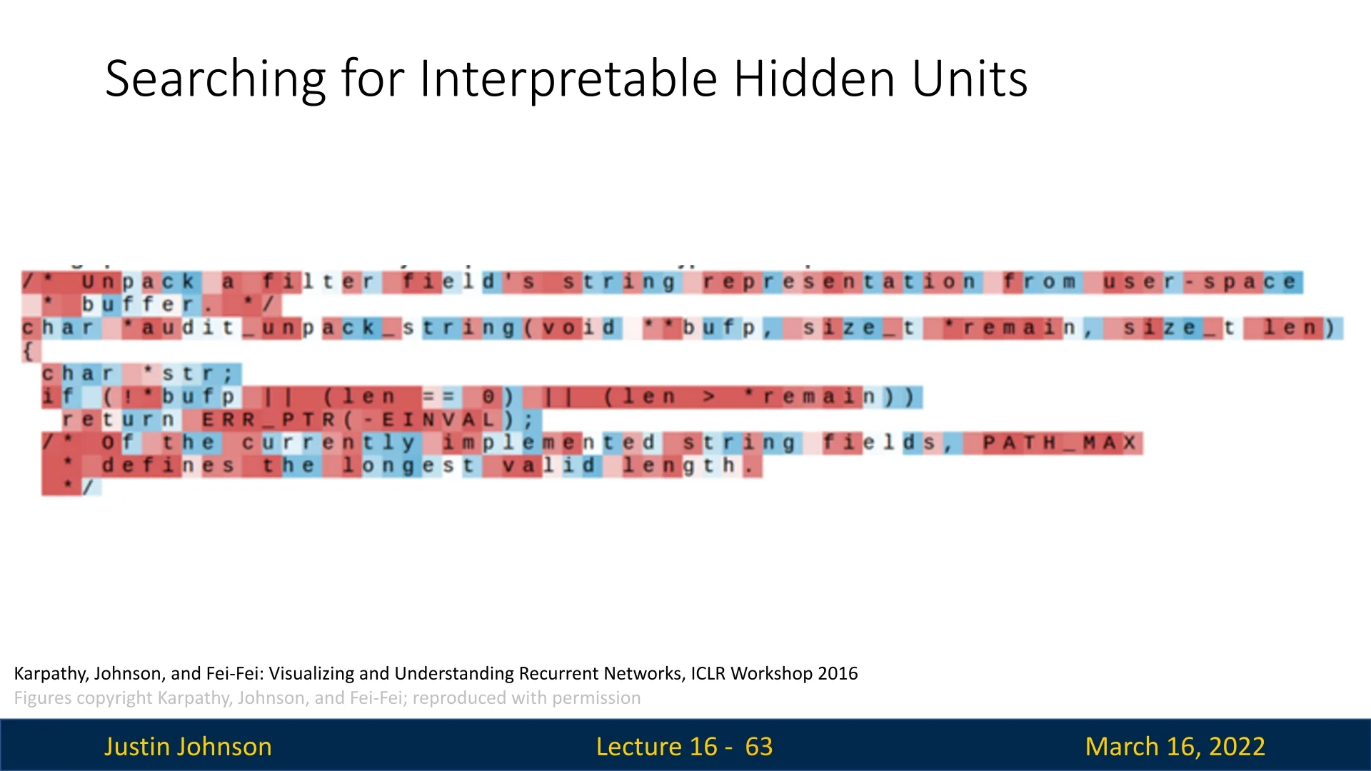
As shown in Figure 16.9, many hidden unit activations appeared random and did not provide an intuitive understanding of what the RNN was tracking. However, in some cases, individual hidden state dimensions exhibited clear, meaningful behavior.
Interpretable Hidden Units
While many hidden state dimensions appear uninterpretable, some exhibit structured activation patterns corresponding to meaningful aspects of the data. Below are a few examples:
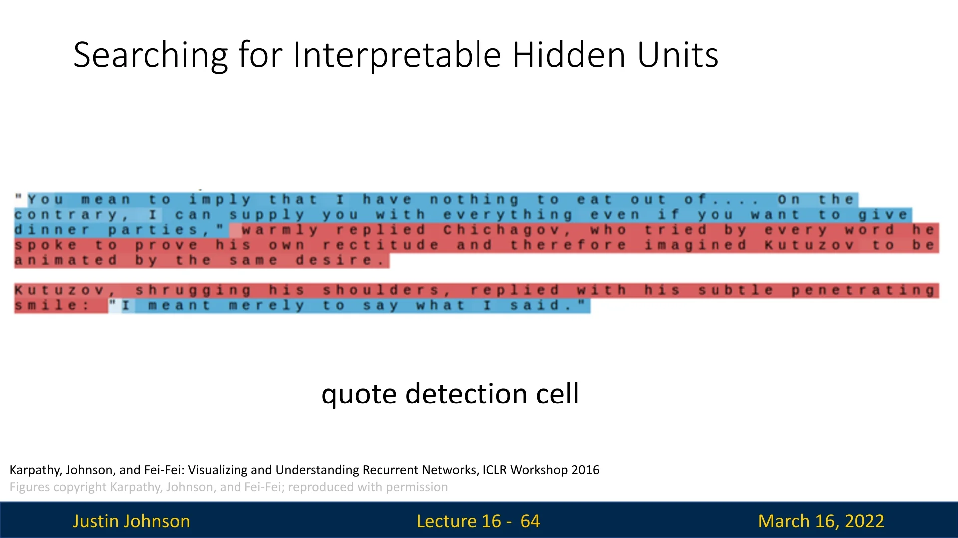
Some hidden units activate strongly in the presence of quoted text, as seen in Figure 16.10.
Line Length Tracking Cell Another hidden unit tracks the number of characters in a line, transitioning smoothly from blue to red as it approaches 80 characters per line (a common convention in code formatting), as shown in Figure 16.11.
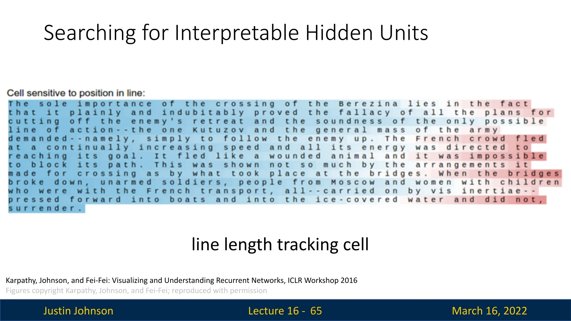
This demonstrates that some RNN neurons track specific long-range dependencies, encoding useful properties of the dataset.
Other meaningful hidden state activations include:
- Comment Detector: Some units activate strongly in commented-out sections of code.
- Code Depth Tracker: Certain units track the depth of nested code structures (e.g., counting how many open brackets exist in C code).
- Keyword Highlighter: Some neurons respond selectively to keywords such as if, for, or return in programming languages.
Key Takeaways from Interpretable Units
The analysis by Karpathy et al. highlights several important insights:
- RNNs can learn abstract properties of sequences. Some hidden units respond to high-level features, such as quoted text, line length, or code structure.
- Not all hidden units are interpretable. Many dimensions in the hidden state vector appear to activate randomly, making it difficult to extract clear meaning from every neuron.
- Neurons behave differently based on the dataset. The same RNN architecture trained on different corpora may develop completely different internal representations.
While these findings provide insight into what RNNs learn, interpreting hidden states remains an open challenge in deep learning research. This motivates further study into techniques such as attention mechanisms and gated architectures, which offer more structured ways to track long-term dependencies.
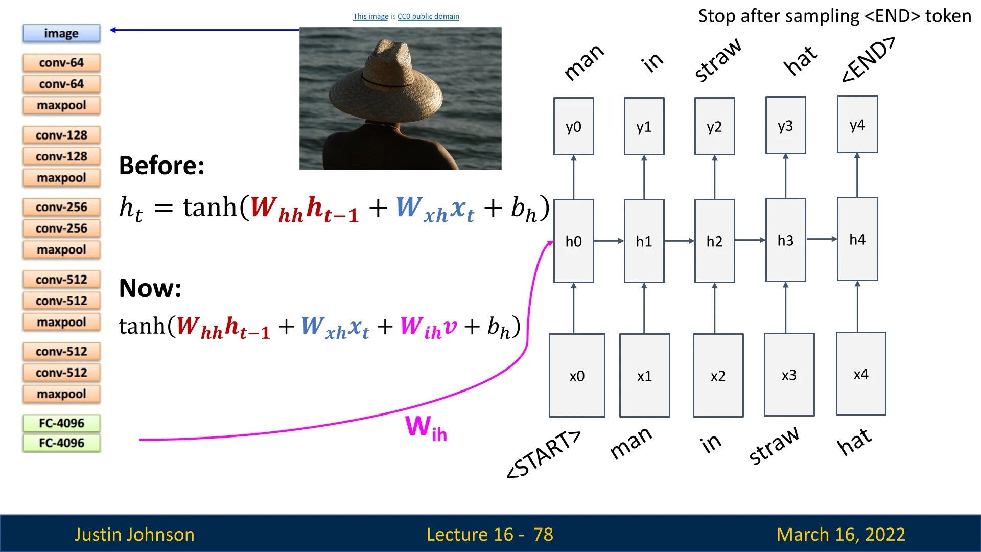
16.6.3 Image Captioning
Image captioning is the task of generating a textual description of an image by combining computer vision (to extract meaningful features) and natural language processing (to generate coherent text). The standard pipeline consists of two main components:
- 1.
- Feature Extraction with a Pre-Trained CNN: A convolutional neural network (CNN), originally trained for image classification (e.g., on ImageNet), is used to encode the image into a high-level feature representation. The final fully connected layers are removed, leaving only/mostly the convolutional layers to produce an image embedding.
- 2.
- Caption Generation with an RNN: The extracted image features serve as additional input to an RNN, which generates a description one word at a time, starting from a special <START> token and stopping at an <END> token.
The standard RNN hidden state update equation: \[ \mathbf {h}_t = \tanh \big ( \mathbf {W}_{xh} \mathbf {x}_t + \mathbf {W}_{hh} \mathbf {h}_{t-1} \big ), \] is modified to incorporate the image features: \[ \mathbf {h}_t = \tanh \big ( \mathbf {W}_{xh} \mathbf {x}_t + \mathbf {W}_{hh} \mathbf {h}_{t-1} + \mathbf {W}_{ih} \mathbf {v} \big ), \] where:
- \( \mathbf {x}_t \) is the current input word,
- \( \mathbf {h}_{t-1} \) is the previous hidden state,
- \( \mathbf {v} \) is the image embedding from the CNN,
- \( \mathbf {W}_{ih} \) learns how to integrate image features into the sequence model.
16.6.4 Image Captioning Results
When trained effectively, RNN-based image captioning models generate descriptions that align well with the content of an image.

Some strengths of the model include:
- Identifying objects and their relationships (e.g., ”a cat sitting on a suitcase”).
- Capturing spatial context within the scene.
- Producing fluent, grammatically correct sentences.
However, the model is limited in its reasoning abilities, often making systematic errors.
16.6.5 Failure Cases in Image Captioning
Despite generating plausible captions, RNN-based models struggle with dataset biases and lack true scene understanding.

Notable failure cases include:
- Texture Confusion: ”A woman is holding a cat in her hand.”
→ Incorrect. The model misinterprets a fur coat as a cat due to similar texture. - Outdated Training Data: ”A person holding a computer mouse on
a desk.”
→ Incorrect. Since the dataset predates smartphones, the model assumes any small handheld object near a desk is a computer mouse. - Contextual Overgeneralization: ”A woman standing on a beach
holding a surfboard.”
→ Incorrect. The model associates beaches with surfing due to frequent co-occurrence in the dataset. - Co-Occurrence Bias: ”A bird is perched on a tree branch.”
→ Incorrect. The model predicts a bird even though none are present, likely due to birds frequently appearing in similar scenes in the dataset. - Failure to Understand Actions: ”A man in a baseball uniform
throwing a ball.”
→ Incorrect. The model fails to distinguish between throwing and catching, highlighting a lack of true scene comprehension.
These errors indicate that RNN-based captioning models rely heavily on statistical associations rather than genuine reasoning. Their fixed-size hidden state struggles to store complex dependencies, and they lack explicit mechanisms to retain and retrieve relevant information over long sequences.
16.6.6 Bridging to LSTMs and GRUs: The Need for Gated Memory
The previous subsection gave a theoretical reason why vanilla RNNs with any scalar activation \(\phi \) face an unavoidable trade-off between stability and long-term memory (Table 16.2). The examples in this section—especially image captioning—show how this trade-off manifests in practice.
In text generation and captioning, a vanilla \(\tanh \)-RNN is usually numerically stable and can capture local statistics (syntax, common phrases, co-occurrence patterns), but it exhibits several task-level limitations:
- Hidden-state bottleneck. At each timestep, all relevant information from the past must be compressed into a single vector \(\mathbf {h}_t\). As sequences grow longer, new inputs overwrite older information, making it hard to remember which objects appeared in the image or how a sentence began.
- Gradient-driven myopia. As discussed in Section 16.5.5, gradients in a vanilla RNN are dominated by nearby timesteps. In captioning, this means the model is trained mainly to get the next few words right; long-range dependencies (for example, maintaining the correct subject over an entire sentence) are only weakly enforced.
- No explicit, controllable memory. The only state is the hidden vector \(\mathbf {h}_t\), updated by the same affine map and nonlinearity at every step. There is no mechanism to preserve some information for many steps while freely updating other parts of the representation, nor a way to decide what to remember and when to forget.
The qualitative failure cases in image captioning (Figures 16.14 and related discussion) are concrete symptoms of these limitations: captions drift toward dataset biases, confuse visually similar textures, and forget earlier context even when the RNN is otherwise well trained and numerically stable.
LSTMs and GRUs address these issues not by changing the activation function, but by changing the structure of the recurrence. As previewed in Section 16.5.5, they introduce:
- An explicit memory state that is updated largely additively, so information (and gradients) can flow with gain close to \(1\) over many timesteps.
- Multiplicative gates that learn when to write new information into memory, when to keep it, and when to erase it, rather than relying on the same fixed update rule at every step.
These gated architectures still use stable nonlinearities such as \(\tanh \) and sigmoid at the unit level, but wrap them in a design that decouples “remembering” from “processing.” The result is a recurrent model that can maintain information over hundreds of steps while remaining numerically robust.
In the next section we will make this concrete by deriving the LSTM cell, showing how its additive memory path and gates implement the constant-error-carousel mechanism, and then introducing the more compact GRU.
16.7 Long Short-Term Memory (LSTM) Overview
Long Short-Term Memory (LSTM) networks, introduced by Hochreiter and Schmidhuber [236], represent a pivotal evolutionary step in sequence modeling. LSTMs, together with related gated RNNs such as GRUs, dominated natural language processing and many time-series applications throughout the 2010s, providing the first robust, general-purpose mechanism for learning long-range dependencies with gradient-based training. As of 2025, however, most new large-scale sequence models—including those deployed on mobile and edge devices—are based on attention and Transformer-style architectures, often with convolutional stems and lightweight, hardware-aware Transformer blocks replacing recurrent layers.
Despite this shift, understanding the LSTM remains highly valuable. Historically, LSTMs were the first widely adopted architecture to explicitly separate memory from nonlinear processing by maintaining an internal cell state that is updated largely additively, while using multiplicative gates to decide when to write, keep, or erase information. This design creates a stable gradient pathway over long sequences, mitigating the vanishing-gradient problem that plagues vanilla RNNs, yet still allowing the network to forget irrelevant context. Conceptually, LSTMs form an important stepping stone toward the gated and residual pathways used in Highway Networks and ResNets, and toward the data-dependent relevance weighting implemented by attention and Transformers, which we study next.
16.7.1 LSTM States and Gating Mechanism
In a vanilla RNN, there is a single hidden state \(\mathbf {h}_t\) that is both the internal memory and the output of the recurrent block. LSTMs separate these roles and maintain two states at each timestep:
- Cell state \(\mathbf {c}_t\): A long-term memory that can carry information across many timesteps with relatively minor modification.
- Hidden state \(\mathbf {h}_t\): A short-term, output-facing representation that interacts with inputs and downstream layers.
Rather than updating \(\mathbf {h}_t\) directly via a fixed affine transformation and nonlinearity, LSTMs introduce a small set of gates that regulate information flow. At time \(t\), given input \(\mathbf {x}_t \in \mathbb {R}^{I}\) and previous hidden state \(\mathbf {h}_{t-1} \in \mathbb {R}^{H}\), they compute:
- A forget gate \(\mathbf {f}_t \in (0,1)^H\), which decides how much of \(\mathbf {c}_{t-1}\) to keep.
- An input gate \(\mathbf {i}_t \in (0,1)^H\), which decides how much new information to write.
- A candidate update \(\mathbf {g}_t \in [-1,1]^H\), which proposes new content to add to the cell.
- An output gate \(\mathbf {o}_t \in (0,1)^H\), which decides how much of the internal memory to expose as \(\mathbf {h}_t\).
These gates are themselves learned nonlinear functions of \((\mathbf {h}_{t-1},\mathbf {x}_t)\), and they are trained jointly with the rest of the network by backpropagation through time.
16.7.2 LSTM Gate Computation
Let the previous hidden state be \(\mathbf {h}_{t-1} \in \mathbb {R}^H\) and the current input be \(\mathbf {x}_t \in \mathbb {R}^I\). To control the flow of information, the LSTM computes four vector-valued quantities that share the same input structure but play different roles: \[ \mathbf {W}_*^{(h)} \in \mathbb {R}^{H \times H}, \quad \mathbf {W}_*^{(x)} \in \mathbb {R}^{H \times I}, \quad \mathbf {b}_* \in \mathbb {R}^H, \qquad * \in \{f,i,g,o\}. \] The gate activations are then \begin {align*} \mathbf {f}_t &= \sigma \!\bigl (\mathbf {W}_f^{(h)} \mathbf {h}_{t-1} + \mathbf {W}_f^{(x)} \mathbf {x}_t + \mathbf {b}_f\bigr ) && \text {(forget gate)}, \\ \mathbf {i}_t &= \sigma \!\bigl (\mathbf {W}_i^{(h)} \mathbf {h}_{t-1} + \mathbf {W}_i^{(x)} \mathbf {x}_t + \mathbf {b}_i\bigr ) && \text {(input gate)}, \\ \mathbf {g}_t &= \tanh \!\bigl (\mathbf {W}_g^{(h)} \mathbf {h}_{t-1} + \mathbf {W}_g^{(x)} \mathbf {x}_t + \mathbf {b}_g\bigr ) && \text {(cell candidate)}, \\ \mathbf {o}_t &= \sigma \!\bigl (\mathbf {W}_o^{(h)} \mathbf {h}_{t-1} + \mathbf {W}_o^{(x)} \mathbf {x}_t + \mathbf {b}_o\bigr ) && \text {(output gate)}. \end {align*}
Each element of \(\mathbf {f}_t\), \(\mathbf {i}_t\), and \(\mathbf {o}_t\) lies in \([0,1]\), and each element of \(\mathbf {g}_t\) lies in \([-1,1]\).
Intuition: Gates as soft masks and signed content. The choice of nonlinearities separates control signals from content.
- Sigmoid Gates As Soft Masks. Sigmoid activations for \(\mathbf {f}_t\), \(\mathbf {i}_t\), and \(\mathbf {o}_t\) make each gate coordinate behave like a differentiable valve in \([0,1]\). A value near \(0\) means “block this channel completely”, a value near \(1\) means “pass this channel unchanged”, and intermediate values implement soft decisions such as “keep roughly \(80\%\) of the old memory while writing a bit of new information”. In particular, elements of \(\mathbf {f}_t\) directly scale the previous cell state \(\mathbf {c}_{t-1}\), so the network can learn coordinates that act as almost-perfect copies over hundreds of timesteps (\(\mathbf {f}_t \approx 1\)) and other coordinates that forget rapidly (\(\mathbf {f}_t \approx 0\)).
- Tanh Candidate As Signed Content. The candidate vector \(\mathbf {g}_t\) carries the content that might be written into memory. Using \(\tanh \) keeps \(\mathbf {g}_t\) zero-centered and bounded in \([-1,1]\), which has two important consequences. First, coordinates of \(\mathbf {g}_t\) can contribute positively or negatively to the cell state, so the LSTM can both reinforce and actively counteract previously stored information, for example reducing the weight of an old topic as the sequence shifts to a new subject. Second, the bounded range prevents uncontrolled growth of the internal memory; without a signed, bounded update, \(\mathbf {c}_t\) would tend to drift or explode over long sequences, making optimization unstable.
In practice, deep learning libraries optimize these computations by vectorizing them. Instead of applying four separate affine transformations, we concatenate the hidden state and input, \[ \mathbf {z}_t = \begin {bmatrix} \mathbf {h}_{t-1} \\ \mathbf {x}_t \end {bmatrix} \in \mathbb {R}^{H+I}, \] and use a single weight matrix and bias: \[ \begin {bmatrix} \mathbf {f}_t \\ \mathbf {i}_t \\ \mathbf {g}_t \\ \mathbf {o}_t \end {bmatrix} = \mathbf {W}\mathbf {z}_t + \mathbf {b}, \qquad \mathbf {W} \in \mathbb {R}^{4H \times (H+I)}, \; \mathbf {b} \in \mathbb {R}^{4H}. \] The resulting \(4H\)-dimensional vector is then split into four blocks and passed through the appropriate nonlinearities: \[ \mathbf {f}_t = \sigma (\cdot ), \quad \mathbf {i}_t = \sigma (\cdot ), \quad \mathbf {g}_t = \tanh (\cdot ), \quad \mathbf {o}_t = \sigma (\cdot ). \] This single-matrix implementation is mathematically equivalent to using separate weights per gate, but it is more efficient on modern hardware and is the default in PyTorch, TensorFlow, JAX, and related frameworks.
Remark (Peephole LSTMs). In the standard LSTM variant above, gates depend only on \(\mathbf {h}_{t-1}\) and \(\mathbf {x}_t\). This means that if the output gate was mostly closed at the previous step (\(\mathbf {o}_{t-1} \approx \mathbf {0}\)), the hidden state \(\mathbf {h}_{t-1}\) may reveal little about the actual contents of the memory cell \(\mathbf {c}_{t-1}\). Peephole connections address this by also feeding \(\mathbf {c}_{t-1}\) into the gate computations, for example: \[ \mathbf {f}_t = \sigma \!\bigl ( \mathbf {W}_f^{(h)} \mathbf {h}_{t-1} + \mathbf {W}_f^{(x)} \mathbf {x}_t + \mathbf {W}_f^{(c)} \mathbf {c}_{t-1} + \mathbf {b}_f \bigr ). \] A convenient way to summarize the design trade-offs is:
Pros.
- Makes gates aware of hidden memory contents. In a standard LSTM, if the output gate is mostly closed (\(\mathbf {o}_{t-1} \approx 0\)), then \(\mathbf {h}_{t-1}\) carries almost no information about what is stored in \(\mathbf {c}_{t-1}\), so the forget and input gates at time \(t\) must decide what to do without really “seeing” the current memory. Peephole connections remove this blind spot by letting each gate look directly at \(\mathbf {c}_{t-1}\) when deciding whether to keep, overwrite, or expose information.
- Enables precise counting and timing. When gates can read \(\mathbf {c}_t\) itself, the cell state can act as an internal counter or clock, increasing by a fixed amount each step until a learned threshold is reached, at which point a gate can reliably open or close. This makes peephole LSTMs well suited for tasks with sharp temporal boundaries or periodic structure, such as waiting for exactly \(N\) steps before emitting a signal or aligning outputs to regular beats.
Cons.
- Peephole connections slightly complicate the architecture and add extra parameters, breaking the clean separation between the internal memory pathway and the externally visible hidden state.
- They marginally complicate efficient vectorized implementations, and empirical gains on common language modeling and translation benchmarks are modest, so most modern libraries default to the simpler peephole-free formulation.
16.7.3 LSTM State Updates and Outputs
Once the gates are computed, the LSTM updates its internal memory (cell state) and its visible output (hidden state) at each timestep \(t\).
Cell state update (additive memory path) The cell state \(\mathbf {c}_t\) is updated by a gated combination of the previous cell state and the candidate update: \[ \mathbf {c}_t = \underbrace {\mathbf {f}_t \odot \mathbf {c}_{t-1}}_{\mbox{Keep selected parts of the past}} + \underbrace {\mathbf {i}_t \odot \mathbf {g}_t}_{\mbox{Write new information into memory}}, \]
where \(\odot \) denotes elementwise multiplication. Intuitively:
- The term \(\mathbf {f}_t \odot \mathbf {c}_{t-1}\) determines which components of the previous memory should be preserved and which should be attenuated.
- The term \(\mathbf {i}_t \odot \mathbf {g}_t\) injects newly computed content into the memory, but only along dimensions where the input gate is open.
Because this update is additive rather than repeatedly multiplying by a recurrent weight matrix, it provides a near-identity pathway when \(\mathbf {f}_t \approx \mathbf {1}\) and \(\mathbf {i}_t \approx \mathbf {0}\). Along such coordinates, information can persist almost unchanged for many timesteps, and gradients can flow backward through time without exponentially vanishing.
The hidden state \(\mathbf {h}_t\) is obtained by filtering a squashed version of the cell state: \[ \mathbf {h}_t = \mathbf {o}_t \odot \tanh (\mathbf {c}_t). \] Here, \(\tanh (\mathbf {c}_t)\) produces a bounded, zero-centered summary of the internal memory, and the output gate \(\mathbf {o}_t\) decides how much of that summary to expose at timestep \(t\).
It is useful to think of \(\mathbf {c}_t\) as long-term memory and \(\mathbf {h}_t\) as working memory that is currently visible to the rest of the network. For a sequence \((\mathbf {x}_1,\dots ,\mathbf {x}_T)\), the update above is applied at every timestep \(t=1,\dots ,T\).
The dual role of \(\mathbf {h}_t\) The hidden state \(\mathbf {h}_t\) serves two roles simultaneously at each timestep \(t\):
- Horizontal (temporal) role. \(\mathbf {h}_t\) is passed forward in time to the next LSTM cell as part of the input for timestep \(t+1\), providing context about everything the model has processed so far.
- Vertical (output) role. \(\mathbf {h}_t\) is also passed upward to subsequent layers or an output head at the same timestep, enabling the network to produce a prediction based on the current context.
Thus, at every timestep the LSTM both updates its internal memory for the future and provides a representation that can be decoded into an output for the present.
From hidden states to predictions
The LSTM cell defines how \((\mathbf {c}_t,\mathbf {h}_t)\) evolve over time, but most learning tasks require predictions \(\hat {\mathbf {y}}_t\) in some output space, such as a vocabulary distribution for language modeling or a real-valued vector for regression. To obtain such predictions, a separate output projection maps the hidden state \(\mathbf {h}_t\) to the desired output: \[ \hat {\mathbf {y}}_t = \varphi \!\bigl (\mathbf {W}_{hy}\mathbf {h}_t + \mathbf {b}_y\bigr ), \] where:
- Parameter \(\mathbf {W}_{hy} \in \mathbb {R}^{D \times H}\) and bias \(\mathbf {b}_y \in \mathbb {R}^D\) are trainable output-layer parameters that map the hidden size \(H\) to an output dimension \(D\).
- Dimension \(D\) is the size of the output space, such as the vocabulary size in language modeling or the number of regression targets.
- Function \(\varphi \) is a task-dependent activation, such as softmax for multiclass classification, identity for regression, or sigmoid for binary outputs.
In autoregressive sequence modeling tasks such as language modeling, this projection is usually applied at every timestep \(t\), producing a distribution \(\hat {\mathbf {y}}_t\) over the next token given the prefix \((\mathbf {x}_1,\dots ,\mathbf {x}_t)\).
In sequence classification tasks (for example, sentiment analysis), it is common to ignore intermediate outputs and apply the projection only to a pooled representation, such as the final hidden state \(\mathbf {h}_T\) or an aggregate of all hidden states.
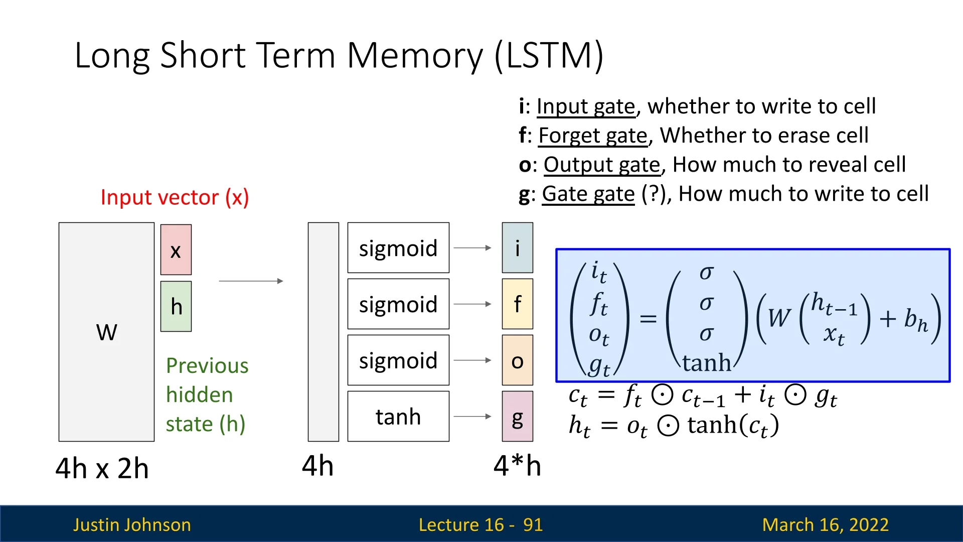
16.7.4 Gradient Flow in LSTMs
Section 16.4 showed that in vanilla RNNs, gradients backpropagated through time are dominated by products of Jacobians of the form \[ \prod _{t} \mathbf {J}_t \quad \mbox{with}\quad \mathbf {J}_t = \mathrm {diag}\bigl (\phi '(\cdot )\bigr )\mathbf {W}_{hh}, \] which either explode or vanish over long horizons depending on the spectrum of \(\mathbf {W}_{hh}\). LSTMs change this picture by introducing an internal cell state \(\mathbf {c}_t\) that is updated additively and does not pass through a recurrent weight matrix at every step. As a result, there is a primary error path that behaves much closer to a near-identity mapping, controlled by the forget gate rather than by repeated multiplication with \(\mathbf {W}_{hh}\).
Cell state as a long-term gradient highway
Recall the cell-state update: \[ \mathbf {c}_t = \mathbf {f}_t \odot \mathbf {c}_{t-1} + \mathbf {i}_t \odot \mathbf {g}_t. \] To study gradient flow, we examine the Jacobian of \(\mathbf {c}_t\) with respect to \(\mathbf {c}_{t-1}\). Using the product rule (and omitting diagonal notation for brevity), we obtain \[ \frac {\partial \mathbf {c}_t}{\partial \mathbf {c}_{t-1}} = \underbrace {\mathbf {f}_t}_{\mbox{direct path}} + \underbrace { \mathbf {c}_{t-1} \odot \frac {\partial \mathbf {f}_t}{\partial \mathbf {c}_{t-1}} + \mathbf {g}_t \odot \frac {\partial \mathbf {i}_t}{\partial \mathbf {c}_{t-1}} + \mathbf {i}_t \odot \frac {\partial \mathbf {g}_t}{\partial \mathbf {c}_{t-1}} }_{\mbox{indirect gate-dependent paths}}. \] The first term, \(\mathbf {f}_t\), is the direct scaling of \(\mathbf {c}_{t-1}\) as it flows into \(\mathbf {c}_t\). The remaining terms capture how changes in \(\mathbf {c}_{t-1}\) influence \(\mathbf {c}_t\) indirectly via changes in the gates.
The key observation is that the indirect terms are always modulated by derivatives of sigmoids or \(\tanh \), which are bounded:
- Sigmoid derivatives satisfy \(\sigma '(z) \leq 0.25\) and quickly approach \(0\) when \(|z|\) is large.
- Tanh derivatives satisfy \(\tanh '(z) \leq 1\) and also approach \(0\) as \(|z|\) grows.
As gradients are propagated backward through many timesteps, these indirect paths involve long products of such small factors and therefore decay rapidly. They act as local corrections that matter over a few steps, but they do not sustain gradients over long horizons.
By contrast, the direct term \(\mathbf {f}_t\) appears without an additional activation derivative in this path. For a loss \(\mathcal {L}\) decomposed as \(\mathcal {L} = \sum _{k=1}^T \mathcal {L}_k\), the dominant contribution to \(\partial \mathcal {L} / \partial \mathbf {c}_t\) along the cell-state chain satisfies \[ \frac {\partial \mathcal {L}}{\partial \mathbf {c}_t} \approx \sum _{k=t}^T \frac {\partial \mathcal {L}_k}{\partial \mathbf {c}_k} \prod _{j=t+1}^k \mathbf {f}_j. \] Because \(\mathbf {f}_j \in (0,1)^H\), each coordinate of the gradient along a specific cell dimension is scaled only by the corresponding coordinate of \(\mathbf {f}_j\). If a particular coordinate of \(\mathbf {f}_j\) is learned to stay close to \(1\) over many steps, then the gradient along that coordinate can travel backward across long time horizons with little attenuation. This mechanism is often referred to as the constant error carousel in the original LSTM paper [236].
Why the forget gate prevents severe vanishing
In a vanilla RNN, the analogue of the forget gate is the Jacobian \[ \frac {\partial \mathbf {h}_t}{\partial \mathbf {h}_{t-1}} = \mathrm {diag}\bigl (\phi '(\cdot )\bigr )\mathbf {W}_{hh}, \] which combines a recurrent weight matrix and activation derivatives that are often much less than \(1\) in magnitude. Repeated multiplication by such matrices quickly drives gradients toward zero or infinity unless \(\mathbf {W}_{hh}\) is carefully constrained.
In an LSTM, the main long-range path is instead governed by \[ \prod _{j=t+1}^{T} \frac {\partial \mathbf {c}_j}{\partial \mathbf {c}_{j-1}} \approx \prod _{j=t+1}^{T} \mathbf {f}_j, \] so gradient preservation is controlled directly by the learned forget gates rather than by the eigenvalues of a shared recurrent matrix. Two properties are crucial:
- The forget gate \(\mathbf {f}_j = \sigma (\cdot )\) is directly parameterized by its own weights and bias, so the network can explicitly learn to keep certain coordinates near \(1\) whenever it is beneficial to store information across long time spans.
- Coordinates that do not need long-term memory can be driven toward \(0\), allowing the network to forget irrelevant information and preventing unnecessary accumulation in the cell state.
Thus, instead of being forced to live near a narrow spectral radius regime of \(\mathbf {W}_{hh}\), the model gains fine-grained, dimension-wise control over how quickly information and gradients decay.
Practical note: forget gate bias initialization In principle, the network should learn to set \(\mathbf {f}_t \approx \mathbf {1}\) on coordinates that ought to store long-term information. However, standard symmetric initialization (weights and biases near zero) yields \(\mathbf {f}_t = \sigma (0) = 0.5\) at the start of training. This means that, before any learning has taken place, both the cell state and its gradients decay by roughly a factor of \(0.5\) per timestep, so after \(T\) steps the signal is attenuated by about \(0.5^T\). For moderately long sequences, this is effectively zero, and the model never receives a strong gradient signal that would tell it to open the forget gate. This is a kind of “chicken-and-egg” problem: the network would like to learn long-term memory, but the gradients needed to learn that behavior vanish too quickly.
A simple and widely used remedy is to initialize the forget gate bias \(\mathbf {b}_f\) to a positive value (for example, all ones or twos) instead of zero. This changes the behavior at initialization in two useful ways:
- It yields \(\mathbf {f}_t \approx \sigma (1) \approx 0.73\) or higher, so the default behavior is closer to an identity mapping along the cell state, and gradients can traverse many timesteps before decaying appreciably.
- It effectively provides an identity skip connection through time, analogous to the residual connections in ResNets, so training starts in a regime with “almost infinite” memory and the model only has to learn when and where to forget, rather than struggling to learn long-term retention from a short-memory initialization.
Hidden-state gradients versus cell-state gradients
The hidden state is given by \[ \mathbf {h}_t = \mathbf {o}_t \odot \tanh (\mathbf {c}_t). \] Its dependence on \(\mathbf {h}_{t-1}\) runs through the gates, which themselves depend on \(\mathbf {h}_{t-1}\) via recurrent weight matrices. Consequently, the Jacobian \[ \frac {\partial \mathbf {h}_t}{\partial \mathbf {h}_{t-1}} \] can still exhibit vanishing or exploding behavior if repeatedly applied, especially in very deep stacks of LSTM layers.
However, LSTMs do not rely solely on this hidden-state Jacobian chain to propagate long-range information. The dominant pathway for long-term dependencies is the additive chain \[ \mathbf {c}_1 \rightarrow \mathbf {c}_2 \rightarrow \dots \rightarrow \mathbf {c}_T, \] whose derivatives are governed primarily by the forget gates \(\mathbf {f}_t\). Even if \(\partial \mathbf {h}_t / \partial \mathbf {h}_{t-1}\) is locally small or large, the model can still preserve and adjust long-term information through the cell state. In other words, the backbone of memory and gradients runs through \(\mathbf {c}_t\), and the hidden-state chain can be viewed as a secondary, more local pathway.
Weight gradients and exploding gradients
During backpropagation, gradients with respect to LSTM parameters receive contributions from both \(\partial \mathbf {h}_t / \partial \mathbf {W}\) and \(\partial \mathbf {c}_t / \partial \mathbf {W}\). Because the derivative of \(\mathbf {c}_T\) with respect to \(\mathbf {c}_t\) is dominated by products of forget gates that can be kept near \(1\), the part of the parameter gradients that flows through the cell state often remains substantial even over long sequences [236, 608]. This means that not all parameter gradients vanish simultaneously, which alleviates one of the central difficulties of training vanilla RNNs.
On the other hand, the gating nonlinearities and \(\tanh \) are bounded, so per-step derivatives rarely exceed \(1\) by a large factor [485]. When occasional large gradients do arise (for example, from the output layer or rare extreme activations), standard gradient clipping can be used as a safeguard. Overall, LSTMs are significantly less prone to catastrophic exploding gradients than vanilla RNNs with unbounded activations, while providing a principled mechanism to preserve gradients over long horizons.
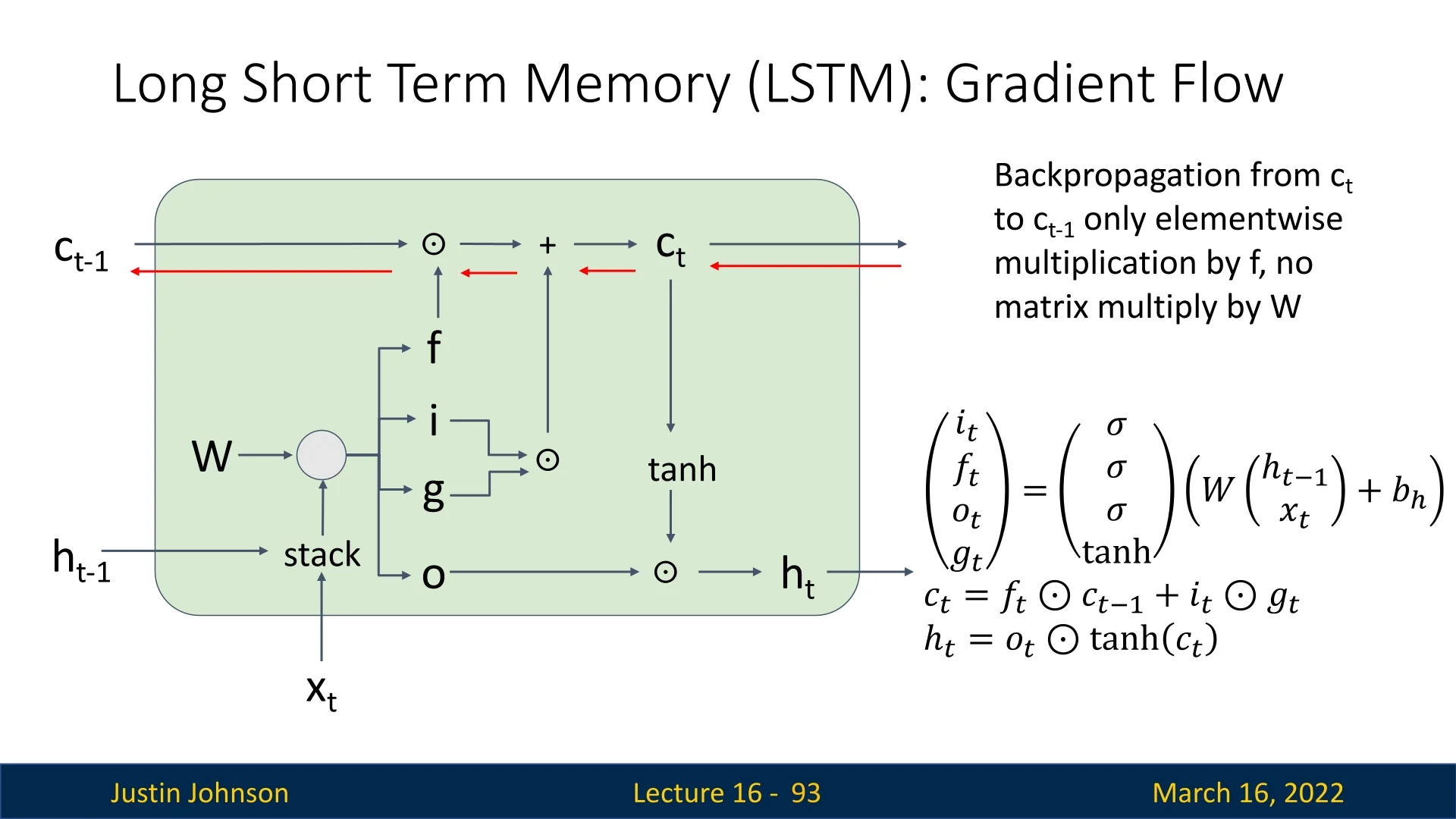
16.8 Resemblance of LSTMs to Highway Networks and ResNets
The central structural idea behind LSTMs is the additive update of an internal state, modulated by gates. This idea closely parallels the developments that later appeared in feedforward architectures, notably Highway Networks [608] and Residual Networks (ResNets) [215].
16.8.1 Highway Networks and LSTMs
Highway Networks introduced gated skip connections between layers, with the basic form \[ \mathbf {y}(x) = T(x) \odot F(x) + \bigl (1 - T(x)\bigr ) \odot x, \] where:
- Transform function \(F(x)\) is a nonlinear mapping (for example, a small MLP) applied to the input \(x\).
- Transform gate \(T(x) = \sigma (\cdot )\) is a trainable gate that decides how much of \(F(x)\) to use.
- Carry gate \(1 - T(x)\) determines how much of the input \(x\) passes through unchanged.
This structure is conceptually very similar to the LSTM cell update \[ \mathbf {c}_t = \mathbf {f}_t \odot \mathbf {c}_{t-1} + \mathbf {i}_t \odot \mathbf {g}_t, \] with \(\mathbf {f}_t\) analogous to the carry gate and \(\mathbf {i}_t\) analogous to the transform gate. In both cases, an additive pathway allows information and gradients to propagate over many layers (or timesteps), while gates decide when to transform and when to copy.
16.8.2 ResNets and LSTMs
ResNets simplify this idea further by using ungated, additive skip connections: \[ \mathbf {x}_{\ell +1} = \mathbf {x}_\ell + F(\mathbf {x}_\ell ). \] This creates a near-identity mapping across layers and dramatically improves gradient flow in very deep networks.
Comparing this with the LSTM cell update: \[ \mathbf {c}_t = \mathbf {f}_t \odot \mathbf {c}_{t-1} + \mathbf {i}_t \odot \mathbf {g}_t, \] we see that both designs share the idea of additive updates as a way to stabilize optimization. ResNets use fixed identity skips (no gates) and are well suited to spatial feature extraction, while LSTMs use gated skips that can adaptively control information flow across time.
- Highway Networks vs. LSTMs. Both use learned gates to interpolate between transformed and carried information, with LSTMs applying this principle along the temporal axis and Highway Networks across depth in feedforward networks.
- ResNets vs. LSTMs. ResNets remove the gates and rely on pure identity skips, trading flexibility for simplicity and scalability to very deep stacks, while LSTMs retain gates to gain fine-grained temporal control over what is remembered or forgotten.
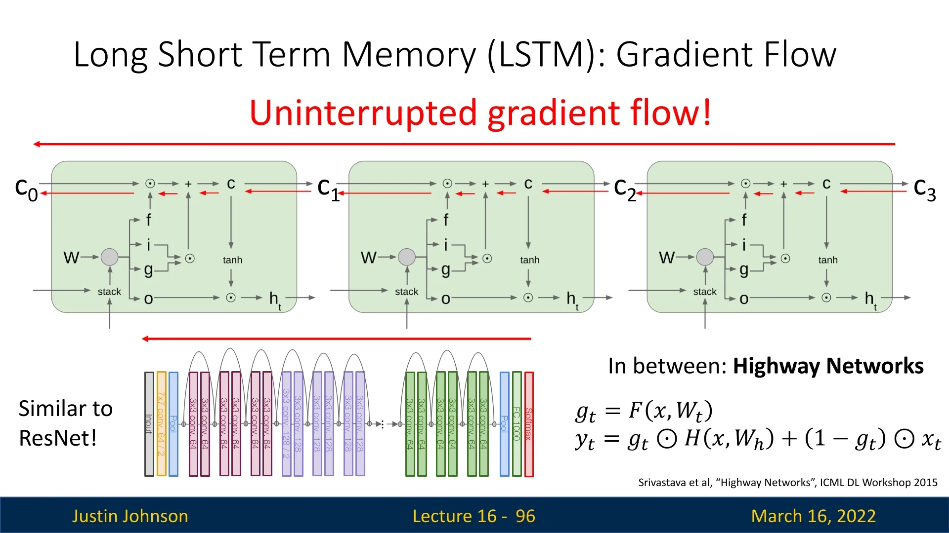
16.8.3 Summary of LSTM, Highway, and ResNet Connections
Viewed in a unified way, LSTMs, Highway Networks, and ResNets all implement variations on the same core theme. They provide an easy, additive path for gradients, and use multiplicative components (gates or residual transforms) to add flexible computation on top. LSTMs apply this pattern in time, Highway Networks across depth with gates, and ResNets across depth with ungated identity connections.
16.9 Bidirectional LSTMs
Standard LSTMs process sequences in a single temporal direction (typically left-to-right). At timestep \(t\), the hidden state \(\mathbf {h}_t\) summarizes only the past inputs \((\mathbf {x}_1,\dots ,\mathbf {x}_t)\), but not the future inputs \((\mathbf {x}_{t+1},\dots ,\mathbf {x}_T)\). This is appropriate for online or autoregressive settings (for example, streaming speech recognition or next-word prediction), but it is suboptimal whenever the entire input sequence is available upfront and decisions should depend on both left and right context.
A classic example is machine translation (for example, English \(\rightarrow \) German) in an encoder–decoder architecture. The encoder receives the full source sentence before the decoder starts producing the target sentence, so in principle it could exploit information from all source tokens when constructing the representation for each position. Unidirectional LSTMs cannot do this: at the position of a source word, they only know the prefix, not the suffix.
Consider the English sentence:
“He turned the heavily protected master switch on.”
To translate this into German, the system must decide at the verb position whether the sense is “rotate” or “switch on”:
- “He rotated the switch.” \(\rightarrow \) Er drehte den Schalter.
- “He turned the switch on.” \(\rightarrow \) Er schaltete den Schalter ein.
A left-to-right LSTM at the word “turned” has seen only the prefix “He turned the heavily protected master switch …”, but not the particle “on”. It must guess between drehte and schaltete without yet seeing the crucial future context. A bidirectional LSTM fixes this by also running a backward LSTM that has already processed the “…switch on” part when constructing the representation at “turned”.
16.9.1 Architecture and information flow
Bidirectional LSTMs (BiLSTMs) address this limitation by running two independent LSTMs over the same sequence:
- A forward LSTM that reads from left to right, \(t = 1 \rightarrow T\), with parameters \(\theta _{\rightarrow }\) and hidden states \(\overrightarrow {\mathbf {h}}_t\).
- A backward LSTM that reads from right to left, \(t = T \rightarrow 1\), with parameters \(\theta _{\leftarrow }\) and hidden states \(\overleftarrow {\mathbf {h}}_t\).
The two LSTMs do not share weights; they are separate networks that see the sequence in opposite directions and can learn different dynamics.
Let the input sequence be \(\mathbf {x}_1,\dots ,\mathbf {x}_T\). For each position \(t\), we can write the recurrences abstractly as \begin {align*} \overrightarrow {\mathbf {h}}_t &= \mathrm {LSTM}_{\rightarrow }\bigl (\mathbf {x}_t, \overrightarrow {\mathbf {h}}_{t-1}, \overrightarrow {\mathbf {c}}_{t-1};\, \theta _{\rightarrow }\bigr ), \quad t = 1,\dots ,T, \\ \overleftarrow {\mathbf {h}}_t &= \mathrm {LSTM}_{\leftarrow }\bigl (\mathbf {x}_t, \overleftarrow {\mathbf {h}}_{t+1}, \overleftarrow {\mathbf {c}}_{t+1};\, \theta _{\leftarrow }\bigr ), \quad t = T,\dots ,1, \end {align*}
where \(\overrightarrow {\mathbf {c}}_t\) and \(\overleftarrow {\mathbf {c}}_t\) are the corresponding cell states. Unrolling these recurrences shows the effective context seen at each timestep:
- The forward state \(\overrightarrow {\mathbf {h}}_t\) summarizes the prefix \(\{\mathbf {x}_1,\dots ,\mathbf {x}_t\}\).
- The backward state \(\overleftarrow {\mathbf {h}}_t\) summarizes the suffix \(\{\mathbf {x}_t,\dots ,\mathbf {x}_T\}\).
Thus, once both passes have been run, the model has, at every position \(t\), two complementary views: one from the left context up to and including \(\mathbf {x}_t\), and one from the right context down to and including \(\mathbf {x}_t\).
16.9.2 Full-context representations at each position
After computing both directional states, a BiLSTM forms a combined representation at each timestep \(t\), typically by concatenation: \[ \mathbf {y}_t = \begin {bmatrix} \overrightarrow {\mathbf {h}}_t \\ \overleftarrow {\mathbf {h}}_t \end {bmatrix}. \] By construction, \(\mathbf {y}_t\) encodes information from the entire sequence: \[ \mbox{Context}(\mathbf {y}_t) = \{\mathbf {x}_1,\dots ,\mathbf {x}_{t-1}\} \cup \{\mathbf {x}_t\} \cup \{\mathbf {x}_{t+1},\dots ,\mathbf {x}_T\}. \]
One useful way to see this is step by step:
- At \(t = 1\), the forward LSTM has seen only \(\mathbf {x}_1\), while the backward LSTM has already processed \(\mathbf {x}_T,\dots ,\mathbf {x}_2,\mathbf {x}_1\), so \(\overleftarrow {\mathbf {h}}_1\) summarizes all remaining words “to the right” of position \(1\).
- At \(t = 2\), the forward LSTM has seen \(\mathbf {x}_1,\mathbf {x}_2\), while the backward LSTM has processed \(\mathbf {x}_T,\dots ,\mathbf {x}_3,\mathbf {x}_2\), so \(\overleftarrow {\mathbf {h}}_2\) summarizes everything from position \(2\) to the end.
- In general, for any \(t\), \(\overrightarrow {\mathbf {h}}_t\) knows the prefix \(\mathbf {x}_1,\dots ,\mathbf {x}_t\) and \(\overleftarrow {\mathbf {h}}_t\) knows the suffix \(\mathbf {x}_t,\dots ,\mathbf {x}_T\), so \(\mathbf {y}_t\) represents \(\mathbf {x}_t\) in the context of the entire sentence.
Returning to the translation example “He turned the heavily protected master switch on.”, suppose we focus on the token “turned”.
- The forward state \(\overrightarrow {\mathbf {h}}_{\mbox{turned}}\) summarizes the prefix “He turned the heavily protected master switch …”, which is still ambiguous between “rotate” and “switch on”.
- The backward state \(\overleftarrow {\mathbf {h}}_{\mbox{turned}}\) has already processed “…master switch on”, and therefore encodes the presence of the particle “on” and the surrounding context.
- The combined vector \(\mathbf {y}_{\mbox{turned}} = [\overrightarrow {\mathbf {h}}_{\mbox{turned}};\overleftarrow {\mathbf {h}}_{\mbox{turned}}]\) can therefore support the correct choice of a German verb such as schaltete rather than drehte.
In other words, at each source position the BiLSTM encoder constructs a representation that already “knows” about future words that may be crucial for a faithful translation.
16.9.3 Using BiLSTM states for predictions
Once \(\mathbf {y}_t\) has been formed, it plays the same role that \(\mathbf {h}_t\) played for a unidirectional LSTM in Section 16.7.3.0. In many pre-Transformer machine translation systems, a BiLSTM was used as the encoder, producing the sequence \(\mathbf {y}_1,\dots ,\mathbf {y}_T\) as a context-rich representation of the source sentence. A decoder (often a unidirectional LSTM) then consumed this sequence directly or via an attention mechanism.
For simpler token-level prediction tasks (for example, part-of-speech tagging or named-entity recognition), a typical choice is a linear output layer with an activation \(\varphi \): \[ \hat {\mathbf {y}}_t = \varphi \!\bigl (\mathbf {W}_y \mathbf {y}_t + \mathbf {b}_y\bigr ), \] where:
- Parameter \(\mathbf {W}_y \in \mathbb {R}^{D \times 2H}\) and bias \(\mathbf {b}_y \in \mathbb {R}^D\) are trainable output-layer parameters.
- Dimension \(2H\) reflects concatenation of the forward and backward hidden states of size \(H\) each.
- Dimension \(D\) is the size of the output space, for example the number of tags in a sequence-labeling task.
For sequence-level prediction (for example, sentence classification), one can aggregate BiLSTM states in several ways, such as:
- Using the concatenation of the last forward state and the first backward state, \([\overrightarrow {\mathbf {h}}_T;\overleftarrow {\mathbf {h}}_1]\).
- Applying max- or mean-pooling over all \(\mathbf {y}_t\) and feeding the pooled vector to a classifier.
16.9.4 Design trade-offs and limitations
BiLSTMs were a standard building block for many pre-Transformer NLP systems and remain conceptually important, but they also introduce specific trade-offs.
Advantages.
- They provide full left-and-right context for each token, which is especially beneficial for disambiguation and structured prediction tasks such as machine translation encoding, part-of-speech tagging, named-entity recognition, chunking, and constituency or dependency parsing.
- They remain relatively easy to integrate into existing LSTM-based architectures, since the forward and backward layers have the same interface as a standard LSTM and differ only in the direction of traversal.
Limitations.
- They are inherently non-causal: computing \(\mathbf {y}_t\) requires access to the entire sequence, so BiLSTMs cannot be used for online or strictly left-to-right generation where future tokens are unknown at prediction time (for example, real-time simultaneous translation).
- They roughly double recurrent computation and memory, since the sequence must be processed once in each direction, and all intermediate states \(\overrightarrow {\mathbf {h}}_t\) and \(\overleftarrow {\mathbf {h}}_t\) must be stored for backpropagation.
In settings where full sequences are available and latency is not dominated by recurrence (for example, offline translation or tagging), these costs are often acceptable. However, in modern practice, many of the benefits of BiLSTMs for capturing bidirectional context have been superseded by self-attention mechanisms and Transformer-style encoders, which provide global context while being more parallelizable across timesteps.
16.10 Stacking Layers in RNNs and LSTMs
Just as feedforward networks and ConvNets benefit from depth, RNNs and LSTMs can be stacked in multiple layers. Each additional recurrent layer operates on the sequence of hidden states produced by the layer below, enabling the model to build increasingly abstract temporal representations.
16.10.1 Architecture of Stacked RNNs and LSTMs
In a stacked RNN or LSTM, the first layer (\(\ell =1\)) reads the raw input sequence \(\{\mathbf {x}_t\}\) and produces hidden states \(\{\mathbf {h}_t^{(1)}\}\). The second layer (\(\ell =2\)) treats \(\{\mathbf {h}_t^{(1)}\}\) as its input sequence and produces \(\{\mathbf {h}_t^{(2)}\}\), and so on: \[ \mathbf {h}_t^{(\ell )} = f^{(\ell )}\Bigl ( \mathbf {h}_t^{(\ell -1)},\, \mathbf {h}_{t-1}^{(\ell )} \Bigr ), \] where \(f^{(\ell )}\) denotes either an RNN or LSTM transition function at layer \(\ell \). For LSTMs, each layer maintains its own cell state \(\mathbf {c}_t^{(\ell )}\) and gates.
The components in this recurrence can be interpreted as follows:
- Hidden state \(\mathbf {h}_t^{(\ell )}\) is the representation at timestep \(t\) in layer \(\ell \).
- Input \(\mathbf {h}_t^{(\ell -1)}\) is the output from layer \(\ell -1\) at time \(t\).
- Previous hidden state \(\mathbf {h}_{t-1}^{(\ell )}\) is the temporal context from the same layer \(\ell \) at the previous timestep.
Lower layers typically capture more local, short-range patterns (for example, character-level statistics or short phrases), while higher layers capture more global, long-range structure (for example, sentence-level semantics). This hierarchy is closely analogous to the way deeper ConvNet layers capture higher-level spatial features.
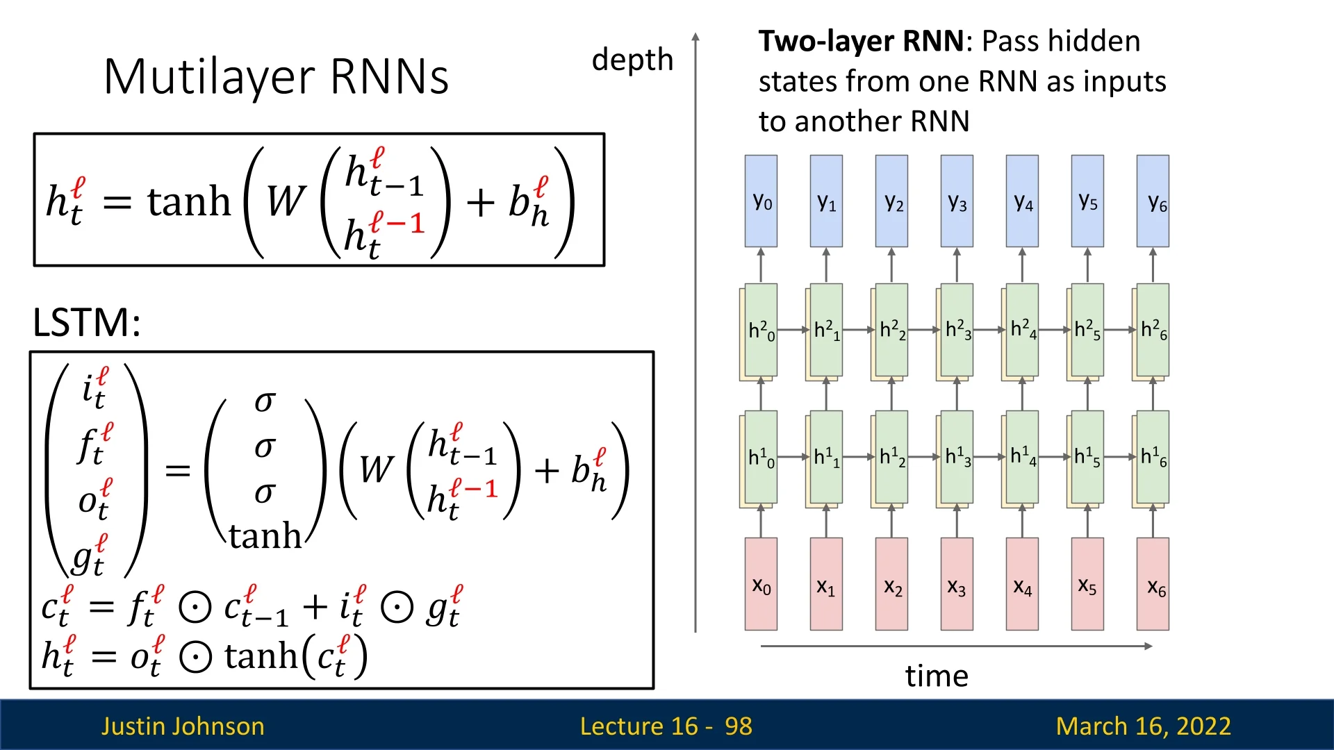
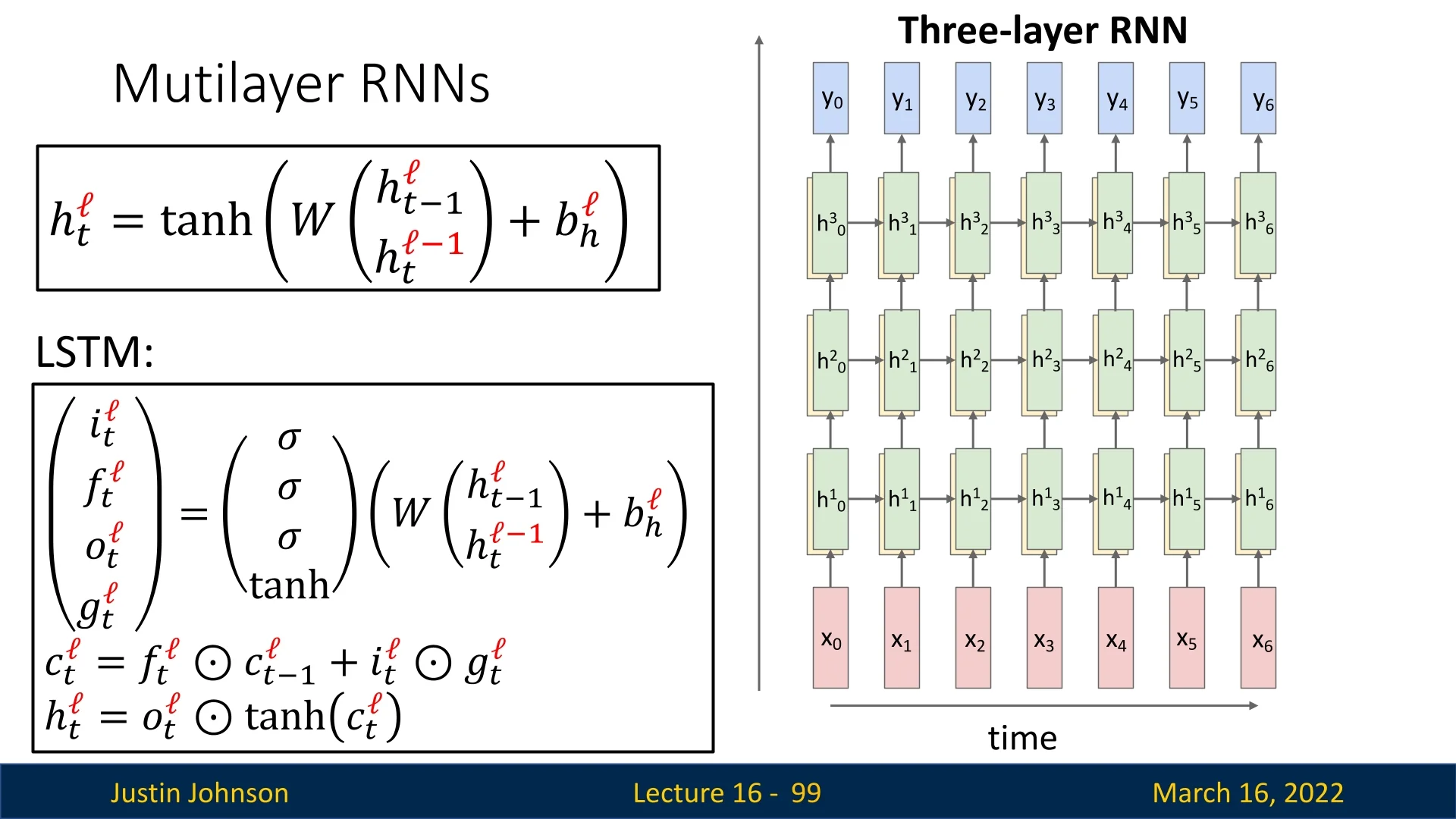
16.10.2 Practical Limitations of Deep Recurrent Stacks
While depth increases representational power, deep recurrent stacks also incur practical costs:
- Diminishing Returns. Beyond a modest number of layers (often 2–4), additional recurrent layers frequently yield only marginal gains, especially when combined with strong regularization and large hidden sizes.
- Overfitting Risk. Each added layer introduces many new parameters, increasing the risk of overfitting unless the dataset is large and regularization (dropout, weight decay, etc.) is carefully tuned.
- Optimization Difficulty. Deeper recurrent stacks are more computationally expensive and can be harder to optimize, even with LSTMs’ improved gradient flow, so gradient clipping and careful initialization become more important as depth grows.
16.10.3 Depth, Directionality, and Efficiency
Stacked RNNs and LSTMs, BiLSTMs, and residual-style connections within recurrent architectures all reflect the same underlying goal: provide sufficient capacity to model complex temporal dependencies, while preserving stable gradient pathways. In practice, many effective architectures combine:
- A small number (2–4) of stacked LSTM or BiLSTM layers.
- Moderate hidden-state sizes.
- Simple output projections as in Section 16.7.3.0.
This combination typically suffices to capture both local and global structure in many sequence modeling tasks, without incurring the severe optimization difficulties that arise in very deep recurrent networks.
Enrichment 16.11: Other RNN Variants: GRU
Gated Recurrent Units (GRUs) [107] are a streamlined yet powerful alternative to Long Short-Term Memory (LSTM) networks, aimed at capturing long-term dependencies while reducing overall architectural complexity. GRUs merge some of the gating components found in LSTMs, thereby reducing parameters and accelerating training, while still offering effective gradient flow for many sequence modeling tasks.
Enrichment 16.11.1: GRU Architecture
GRUs compress the LSTM’s three gates (input, forget, and output) into two gates:
- Reset gate \(r_t\): Controls how much of the previous hidden state \(\mathbf {h}_{t-1}\) is “forgotten” or “reset” before computing a new candidate.
- Update gate \(z_t\): Balances new candidate information against the existing hidden state, effectively merging the “input” and “forget” gating roles found in LSTMs.
Formally, a GRU evolves its hidden state as follows: \[ \begin {aligned} r_t &= \sigma \bigl (\mathbf {W}_{xr} \,\mathbf {x}_t \;+\; \mathbf {W}_{hr} \,\mathbf {h}_{t-1} \;+\; \mathbf {b}_r\bigr ), \\ z_t &= \sigma \bigl (\mathbf {W}_{xz} \,\mathbf {x}_t \;+\; \mathbf {W}_{hz} \,\mathbf {h}_{t-1} \;+\; \mathbf {b}_z\bigr ), \\ \tilde {h}_t &= \tanh \Bigl (\mathbf {W}_{xh}\,\mathbf {x}_t \;+\; \mathbf {W}_{hh}\,\bigl (r_t \odot \mathbf {h}_{t-1}\bigr ) \;+\; \mathbf {b}_h\Bigr ), \\ \mathbf {h}_t &= \bigl (1 - z_t\bigr )\odot \mathbf {h}_{t-1} \;+\; z_t \odot \tilde {h}_t. \end {aligned} \]
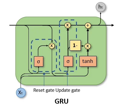
Key observations and intuition
- Coupled “remember–update” behavior. The hidden-state update can be written with an explicit decomposition: \[ \mathbf {h}_t = \underbrace {\bigl (1 - z_t\bigr )\odot \mathbf {h}_{t-1}}_{\mbox{retain old features}} + \underbrace {z_t \odot \tilde {h}_t}_{\mbox{write new features}}. \] Each component of \(z_t\) lies between \(0\) and \(1\), so every dimension of \(\mathbf {h}_t\) is a convex combination of its old value and the candidate. Unlike an LSTM, where the input and forget gates are independent, a GRU couples remembering and updating: to strongly write new content in a dimension (\(z_t \approx 1\)), the model must simultaneously reduce the contribution of the old content (\(1 - z_t \approx 0\)).
- Exposed memory (no separate cell state). LSTMs distinguish between an internal cell state \(\mathbf {c}_t\) and an output \(\mathbf {h}_t\) controlled by an output gate. GRUs remove this distinction: the hidden state \(\mathbf {h}_t\) itself serves as both memory and output. Whatever the GRU remembers at time \(t\) is immediately visible to downstream layers.
- Reset gate as a relevance filter. The reset gate \(r_t\) appears inside the candidate computation: \[ \tilde {h}_t = \tanh \Bigl (\mathbf {W}_{xh}\,\mathbf {x}_t + \mathbf {W}_{hh}\bigl (r_t \odot \mathbf {h}_{t-1}\bigr ) + \mathbf {b}_h\Bigr ). \] When \(r_t \approx 0\), the GRU computes \(\tilde {h}_t\) almost as if the sequence were starting fresh at timestep \(t\), ignoring most of \(\mathbf {h}_{t-1}\). When \(r_t \approx 1\), the full previous state participates in forming new features. This allows the GRU to selectively “break” short-term dependencies (for example, at sentence boundaries) while still maintaining long-range structure in dimensions where \(r_t\) stays high.
This design merges LSTM’s separate input and forget gates into the single update gate \(z_t\), simplifying the gating mechanism while retaining enough flexibility to capture rich temporal structure [107].
Enrichment 16.11.2: Gradient Flow in GRUs
Despite having fewer gates than LSTMs, GRUs preserve stable gradient flow in a way similar to LSTMs, preventing the repeated-multiplication issues that plague vanilla RNNs.
Why GRUs improve over vanilla RNNs
In vanilla RNNs, the hidden state update \[ \mathbf {h}_t = \phi (\mathbf {W}_{hh}\,\mathbf {h}_{t-1} + \dots ) \] causes gradients to vanish or explode through repeated application of \(\mathbf {W}_{hh}\) and the activation derivatives \(\phi '(\cdot )\). In a GRU, large parts of the gradient flow pass through the update mechanism \[ \mathbf {h}_t = (1-z_t)\odot \mathbf {h}_{t-1} + z_t\odot \tilde {h}_t, \qquad \tilde {h}_t = \tanh \Bigl (\mathbf {W}_{xh}\,\mathbf {x}_t + \mathbf {W}_{hh}(r_t\odot \mathbf {h}_{t-1}) + \mathbf {b}_h\Bigr ). \] Differentiating with respect to \(\mathbf {h}_{t-1}\) yields \[ \frac {\partial \mathbf {h}_t}{\partial \mathbf {h}_{t-1}} = \underbrace {\mathrm {diag}(1 - z_t)}_{\mbox{direct additive path}} + \underbrace {\mbox{terms involving } z_t',\, r_t',\, \tanh '(\cdot )}_{\mbox{indirect gated paths}}. \] The first term, \(\mathrm {diag}(1 - z_t)\), is the direct route by which gradients travel from \(\mathbf {h}_t\) back to \(\mathbf {h}_{t-1}\), and it does not involve multiplication by \(\mathbf {W}_{hh}\). The remaining terms include derivatives of sigmoids and \(\tanh \), whose magnitudes are bounded and typically smaller. Over long time horizons, these indirect terms tend to shrink, while the direct path governed by \(1 - z_t\) can remain close to an identity mapping.
Intuitively, each component of \(z_t\) lies between \(0\) and \(1\), so the model can learn:
- \(z_t \approx 0\): keep \(\mathbf {h}_t \approx \mathbf {h}_{t-1}\), yielding a nearly perfect memory and a near-identity Jacobian for that dimension.
- \(z_t \approx 1\): overwrite \(\mathbf {h}_{t-1}\) with \(\tilde {h}_t\), effectively resetting that dimension while still keeping derivatives bounded through the \(\tanh \) nonlinearity.
This mirrors the “constant error” intuition of the LSTM cell state: GRUs create a trainable, dimension-wise near-identity path for gradients, but through \(\mathbf {h}_t\) rather than a separate \(\mathbf {c}_t\).
Reset gate’s gradient role
The reset gate \(r_t\) shapes how the old hidden state \(\mathbf {h}_{t-1}\) influences the candidate \(\tilde {h}_t\): \[ \tilde {h}_t = \tanh (\dots + \mathbf {W}_{hh}\,(r_t \odot \mathbf {h}_{t-1})), \qquad \frac {\partial \tilde {h}_t}{\partial \mathbf {h}_{t-1}} = \tanh '(\dots )\,\mathbf {W}_{hh}\,\mathrm {diag}(r_t). \] Each component of \(r_t\) lies between \(0\) and \(1\), and \(|\tanh '(z)| \le 1\), so this product remains bounded. When \(r_t\) is small, the candidate \(\tilde {h}_t\) and its gradients depend little on \(\mathbf {h}_{t-1}\); when \(r_t\) is large, the past state participates more strongly. Thus \(r_t\) controls how much of the old representation contributes to new feature extraction, without creating unchecked gradient growth.
Comparing GRU to LSTM gradient paths
LSTMs separate memory into a cell state \(\mathbf {c}_t\) and an output state \(\mathbf {h}_t\), and the additive update of \(\mathbf {c}_t\) provides a clear long-range gradient highway. GRUs unify memory and output in \(\mathbf {h}_t\), but the update rule \[ \mathbf {h}_t = (1 - z_t)\odot \mathbf {h}_{t-1} + z_t\odot \tilde {h}_t \] still yields an additive Jacobian component that can be close to the identity whenever \(z_t\) is small. In both architectures, long-term gradients can propagate primarily along these additive paths, avoiding repeated multiplication by the full \(\mathbf {W}_{hh}\) at every step and thereby stabilizing training over longer sequences than vanilla RNNs.
Practical note: update gate bias initialization As with the LSTM forget gate, sensible initialization of the GRU update gate is important for gradient flow. With the convention used here, \[ \mathbf {h}_t = (1 - z_t)\odot \mathbf {h}_{t-1} + z_t \odot \tilde {h}_t, \] small values of \(z_t\) preserve history (since \(\mathbf {h}_t \approx \mathbf {h}_{t-1}\)), whereas large values of \(z_t\) overwrite the old state with new content. If the update gate bias is initialized to zero, then \(z_t = \sigma (0) \approx 0.5\) at the start of training, so each dimension of \(\mathbf {h}_t\) becomes a 50/50 mixture of old and new content, which still leads to noticeable decay over many timesteps.
To encourage a near-identity path initially, a common heuristic under this convention is to initialize the update gate bias \(\mathbf {b}_z\) to a negative value (for example, \(-1\) or \(-2\)), pushing \(z_t = \sigma (\mathbf {b}_z)\) toward smaller values and making the initial dynamics closer to \(\mathbf {h}_t \approx \mathbf {h}_{t-1}\). This provides a default “skip connection” through time and lets the network learn when and where to increase \(z_t\) to overwrite memory, rather than having to discover long-term retention from a strongly mixing initialization.
Enrichment 16.11.3: Advantages of GRUs over LSTMs
GRUs offer several key advantages [107]:
- Computational efficiency: Fewer gates and parameters lead to faster training and reduced memory usage, benefitting resource-constrained applications.
- Comparably strong performance: For many tasks and moderate sequence lengths, GRUs match or slightly exceed LSTM performance, especially when data or compute are limited.
- Simplicity of implementation: With fewer gating components, GRUs are often easier to code, tune, and interpret in terms of gating patterns.
Enrichment 16.11.4: Limitations of GRUs
Despite these advantages:
- Reduced capacity: Merging input and forget behavior into a single update gate can hamper modeling of extremely subtle or highly specialized long-term relationships, where LSTMs’ separate cell state and output gate can provide finer control.
- Hyperparameter sensitivity: Choosing hidden size, learning rates, or initial gate biases remains crucial. In certain problems, a suboptimal initialization can degrade performance more than in LSTMs.
- Less granular control: By combining forget and input gating into \(z_t\), GRUs provide a single mixture path. This can be less fine-grained than the distinct additive cell state in LSTMs, especially for tasks that resemble counting or require very sharp, long-range triggers.
Enrichment 16.11.5: Comparison with LSTMs
Comparing GRUs and LSTMs highlights both shared principles and structural differences:
- Gradient behavior: Both architectures mitigate vanishing and exploding gradients far better than vanilla RNNs by introducing gated, additive update paths (the LSTM cell state \(\mathbf {c}_t\) and the GRU update rule for \(\mathbf {h}_t\); see the gradient-flow enrichments in this chapter).
- Memory representation: LSTMs explicitly separate internal memory \(\mathbf {c}_t\) from the exposed hidden state \(\mathbf {h}_t\), whereas GRUs unify memory and output in \(\mathbf {h}_t\). This makes LSTMs slightly more expressive for tasks needing protected long-term storage, and GRUs simpler for many everyday applications.
- Architectural complexity: GRUs have two gates (reset and update) and no explicit cell state or output gate, leading to fewer parameters and somewhat lower computational cost. LSTMs have three gates and a separate cell state, offering more knobs to tune information flow at the cost of additional complexity.
Thus, both LSTMs and GRUs significantly improve gradient stability over vanilla RNNs. GRUs are often chosen in resource-limited scenarios or when the simpler gating mechanism suffices, whereas LSTMs may still prove stronger on tasks demanding very nuanced, long-distance representations or precise temporal control.
Enrichment 16.11.6: Bridging to Advanced Architectures
While GRUs and LSTMs have significantly enhanced the training stability and effectiveness of recurrent neural networks, their architectures are still manually designed and may not be optimal for every task. Furthermore, despite their improved gradient flow, certain long-term dependencies or more complex patterns may still pose challenges.
To explore alternatives, researchers have introduced methods such as Neural Architecture Search (NAS), which automatically discover recurrent architectures optimized for specific tasks. NAS algorithms systematically explore the design space, identifying architectures that might combine beneficial aspects of GRUs, LSTMs, and other variants, resulting in even more efficient and powerful models.
16.12 Summary and Future Directions
16.11.1 Neural Architecture Search for Improved RNNs
Despite the effectiveness of manually designed recurrent architectures such as LSTMs and GRUs, significant efforts continue in searching for potentially superior designs using automated methods. Neural Architecture Search (NAS) systematically explores vast spaces of candidate architectures using techniques such as evolutionary algorithms or reinforcement learning.
For example, Zoph and Le [831] evaluated approximately 10,000 candidate recurrent architectures, identifying configurations that marginally improved upon traditional LSTMs. However, despite extensive computational investment, these improvements were relatively modest, underscoring that LSTMs and GRUs are already well-tuned architectures with robust performance.
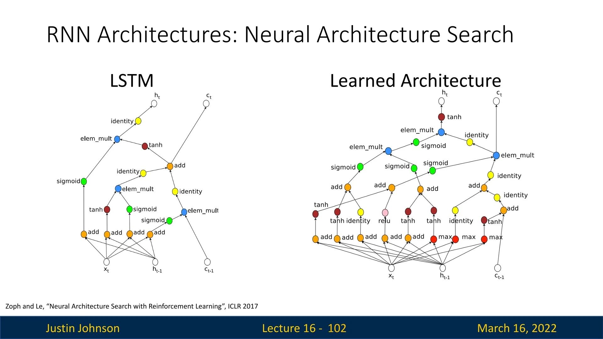
16.11.2 Summary of RNN Architectures
Throughout this chapter, we have explored key architectures developed to overcome challenges inherent to vanilla RNNs, particularly vanishing and exploding gradients:
- Vanilla RNNs: Introduced fundamental recurrence, but are significantly constrained by unstable gradients, limiting their practical effectiveness for capturing long-term dependencies.
-
LSTMs and GRUs: Revolutionized recurrent architectures by employing gating mechanisms and additive state updates, improving gradient stability and long-range dependency modeling:
- LSTMs: Offer explicit gating (input, forget, and output) and an additive cell state, making them robust in capturing intricate and long-term patterns.
- GRUs: Combine gating mechanisms into fewer components, providing computational efficiency and strong performance on many tasks, especially in limited-data or resource-constrained environments, albeit with slightly reduced representational flexibility compared to LSTMs.
- Gradient management: Exploding gradients are effectively controlled by gradient clipping, whereas vanishing gradients are mitigated through gating and additive updates introduced by LSTMs and GRUs.
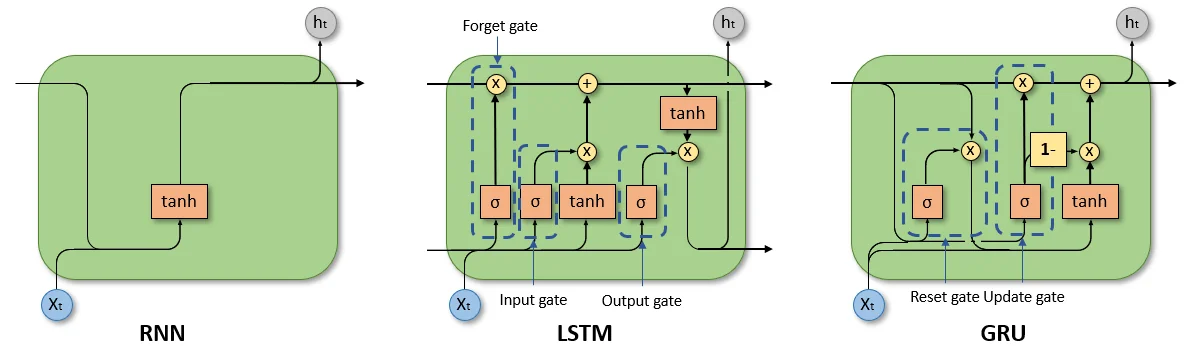
16.11.3 Beyond RNNs: From Recurrence to Attention
Although gating mechanisms greatly enhanced sequence modeling, recurrent architectures inherently rely on sequential computations, making parallelization difficult and hindering performance on extremely long sequences.
Recent developments have introduced attention mechanisms, particularly the Transformer architecture [664], which eliminate recurrence altogether. Transformers employ multi-head self-attention, enabling parallel processing and more effectively capturing extensive contextual relationships within data sequences. This represents a significant advancement, improving both modeling capabilities and computational efficiency.
In the upcoming chapter, we will delve deeply into attention and Transformer architectures, exploring how they address the limitations of RNN-based models and achieve state-of-the-art results in a broad range of sequence modeling tasks.