Lecture 4: Regularization & Optimization

4.1 Introduction to Regularization

In the previous chapter, we explored loss functions as tools to evaluate the performance of machine learning models. However, machine learning is not just about minimizing the loss on the training data. In practice, this narrow focus can be counterproductive, leading to a phenomenon known as overfitting.

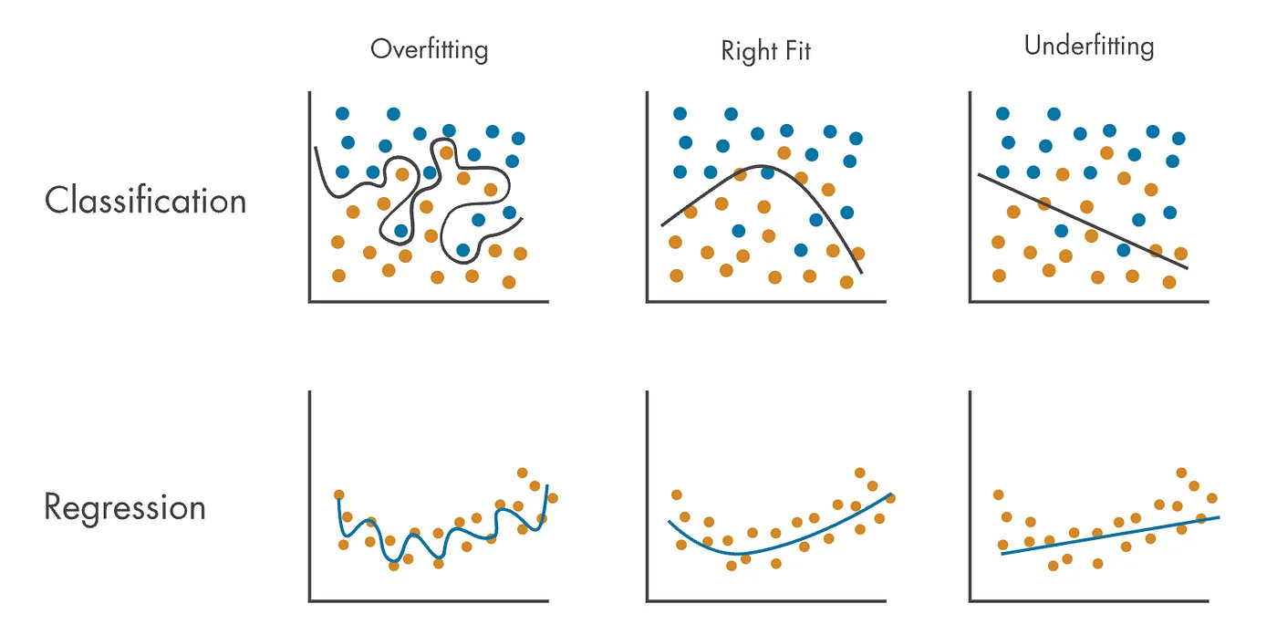
As shown in Figure 4.1, overfitting occurs when a model fits the training data too perfectly, capturing even noise and idiosyncrasies that do not generalize to unseen data. While this may result in excellent performance on the training set, it undermines the model’s ability to perform well on test data or real-world scenarios.

Conversely, underfitting happens when the model is too simplistic to capture the underlying structure of the data, resulting in poor performance on both the training and test sets. Good regularization techniques aim to achieve a balance, ensuring the model fits the data ”just right”.

Why Regularization? The primary purpose of regularization is to improve the model’s generalization—its ability to perform well on unseen data—by discouraging it from overfitting to the training set. However, regularization serves other key roles:

• Improving Optimization: Regularization can add curvature to the loss surface, making optimization easier and more stable.
• Expressing Model Preferences: Beyond simply minimizing training error, regularization allows us to encode preferences for simpler or more interpretable models.

In this chapter, we will dive into various regularization techniques, explore their mathematical foundations, and discuss how they help achieve better generalization. We will also revisit optimization, introducing practical methods to efficiently minimize loss functions in the presence of regularization.

4.1.1 How Regularization is Used?

As discussed in the introduction, in optimization tasks, the goal is to minimize a loss function \( L_\mbox{loss}(W) \), which measures the model’s performance on training data. However, focusing solely on minimizing \( L_\mbox{loss}(W) \) can lead to overfitting, where the model memorizes the training data instead of learning patterns that generalize to unseen data.

Regularization addresses this by adding a penalty term \( R(W) \) to the optimization objective: \[ \mbox{Objective} = \min _W \left [ L_\mbox{loss}(W) + \lambda R(W) \right ], \] where:

• \( \lambda \) is the regularization strength, a hyperparameter controlling the penalty’s weight.
• \( R(W) \) is the regularization term, typically a function of the model weights \( W \), independent of the training data.

4.1.2 Regularization: Encouraging Simpler Models

Without regularization, a network may inflate certain weights to perfectly fit the training data, including noise or outliers. This leads to overfitting and unstable predictions. By adding a penalty term \( R(W) \) to the loss, we encourage the model to prefer simpler parameter configurations, trading off raw accuracy for better generalization: \[ L(W) = L_{\mbox{loss}}(W) + \lambda R(W), \] where \( \lambda \) controls how strongly simplicity is favored.

Here, the optimizer—the algorithm that updates the model’s parameters based on the gradients of \( L(W) \)—must now balance two objectives: minimizing the training error \( L_{\mbox{loss}} \) while keeping the model weights small enough to avoid overfitting. In practice, the optimizer (e.g., SGD or Adam) determines how parameters move through the loss landscape, whereas the regularization term shapes where they tend to settle—toward flatter, simpler solutions that generalize better.

Two widely used choices for \( R(W) \) are L1 and L2 regularization, which differ in how they measure the magnitude of the weights. L1 uses the absolute value (\(|W|\)), encouraging sparsity by driving some weights exactly to zero, while L2 uses the squared value (\(W^2\)), smoothly shrinking all weights toward smaller magnitudes. Both discourage excessive complexity but influence optimization dynamics in distinct ways.

In the following parts, we will see how these forms of regularization shape the optimization process and affect sparsity and generalization.

4.2 Types of Regularization: L1 and L2

4.2.1 L1 Regularization (Lasso)

• Definition: Adds a penalty proportional to the sum of the absolute values of the weights: \[ R(W) = \sum _{i} |w_i|. \]

• Effects:

  • Promotes sparsity by driving many weights to exact zeros, effectively performing feature selection.
  • Encourages interpretable models by retaining only a subset of the most relevant features.

• Why L1 Produces Sparse Weights:

  The key to L1-induced sparsity lies in the geometry of its constraint region. As shown in Figure [fig], the L1 norm constraint \( |w_1| + |w_2| = c \) defines a diamond-shaped region bounded by straight lines. This shape results from the fact that the absolute value function grows linearly and independently in each coordinate.

  When minimizing a loss function subject to this constraint (with an L1 regularization penalty), the optimal solution is often found at the corners of the diamond—points where one or more weights are exactly zero. This happens because these corners offer more degrees of freedom to satisfy the constraint while minimizing the loss.

  Geometrically, the corners of the L1 ball intersect the level sets of the loss function more frequently than the flat sides or interior. As a result, the optimizer is more likely to converge to a solution where some weights are zero, naturally promoting sparsity.

  In contrast, the L2 norm constraint \( w_1^2 + w_2^2 = c^2 \), shown as a circle in the same figure, imposes a smooth, symmetric penalty in all directions. It penalizes large weights more heavily but does not inherently prefer exact zeros. Therefore, L2 regularization tends to shrink weights uniformly rather than forcing them to zero.

  This difference is why L1 regularization (as in Lasso) is often used when feature selection or sparse model representations are desired.

• Pros:

  • Suitable for feature selection in high-dimensional datasets.
  • Produces interpretable models with fewer active features.

• Cons:

  • Struggles with correlated features, arbitrarily selecting one over others.
  • May exclude relevant features if sparsity is overly enforced.

4.2.2 L2 Regularization (Ridge)

• Definition: Adds a penalty proportional to the sum of the squared weights: \[ R(W) = \sum _{i} w_i^2. \]

• Effects:

  • Reduces all weights uniformly, discouraging large weights without enforcing sparsity.
  • Promotes balanced use of all features, making the model less sensitive to individual feature noise.

• Why L2 Regularization Is Common in Practice:

  L2 regularization adds a quadratic penalty term \( \lambda \| \mathbf {w} \|_2^2 = \lambda \sum _j w_j^2 \) to the loss function, which encourages smaller but nonzero weights. This smooth penalty leads to several practical advantages:

  • Smooth optimization landscape: The squared term is differentiable everywhere and convex, making it highly compatible with gradient-based optimization methods. The gradient is simply \( \nabla _{w_j} \left ( \lambda w_j^2 \right ) = 2\lambda w_j \), which leads to stable updates and faster convergence.
  • Weight sharing across correlated features: When input features are correlated, L2 tends to distribute weights more evenly among them rather than forcing the model to pick one arbitrarily. This ”weight spreading” reduces variance and often improves generalization.
  • No bias toward zeroing weights: Unlike L1, L2 does not create sharp corners in the constraint geometry, so weights are shrunk smoothly but rarely exactly zero. This makes it ideal when all features are believed to carry some signal.

• Pros:

  • Retains all features: Useful when input features are all informative, even if weakly.
  • Robust to multicollinearity: When features are correlated, L2 avoids instability by distributing weight mass.
  • Efficient for high-dimensional problems: Closed-form solutions exist for linear models, and gradients are well-behaved for neural networks.

• Cons:

  • No sparsity or feature selection: L2 shrinks weights but rarely sets them exactly to zero, so it cannot be used to remove irrelevant features.

4.2.3 Choosing Between L1 and L2 Regularization

The choice depends on the problem:

• Use L1 Regularization when:

  • Feature selection is essential.
  • A sparse model is required for interpretability.

• Use L2 Regularization when:

  • Features are correlated, and balance is important.
  • Smooth optimization is desired.

Enrichment 4.2.4: Can We Combine L1 and L2 Regularization?

---

Yes! Elastic Net is a regularization technique that combines both L1 (Lasso) and L2 (Ridge) regularization penalties. Its objective function includes a linear combination of the L1 and L2 penalties, defined as:

\[ L(W) = L_\mbox{loss} + \lambda _1 \sum _{i} |w_i| + \lambda _2 \sum _{i} w_i^2, \]

where \(\lambda _1\) controls the L1 penalty, and \(\lambda _2\) controls the L2 penalty. This combination allows Elastic Net to enjoy the benefits of both regularization methods:

• The L1 penalty encourages sparsity, making Elastic Net useful for feature selection by reducing irrelevant feature weights to zero.
• The L2 penalty helps distribute weights among correlated features, overcoming L1’s tendency to select only one feature from a group of highly correlated features.

When to Use Elastic Net? Elastic Net combines both L1 and L2 penalties and is particularly useful when the data exhibits a mix of sparsity and feature correlation. It is especially effective when:

• The dataset has many features, some of which are irrelevant or redundant — L1 encourages sparsity by zeroing out unimportant weights.
• Groups of correlated features contribute jointly to prediction — L2 helps distribute weights across them instead of selecting just one.

By tuning the L1–L2 mixing ratio (commonly via a hyperparameter \( \alpha \)), Elastic Net interpolates smoothly between pure Lasso and pure Ridge behavior.

When Not to Use Elastic Net? Elastic Net may be unnecessary or suboptimal in the following cases:

• When no sparsity is desired: If all features are known to be relevant (e.g., physical signals, embedded representations), L2 regularization (Ridge) is simpler and more appropriate.
• When features are uncorrelated and sparse: Lasso alone may suffice and offer cleaner interpretability without the additional complexity of mixing two norms.
• For very large-scale models or deep learning: Elastic Net adds tuning complexity (both \( \lambda \) and \( \alpha \)) and often doesn’t yield significant benefits over standard L2, which is better understood, easier to optimize, and integrates seamlessly into stochastic gradient descent pipelines.

Summary: Elastic Net strikes a balance between L1 and L2 regularization, making it well-suited for situations where both sparsity and weight sharing are desirable. However, L2 regularization remains the most widely used in practice due to its computational simplicity, smooth gradients, and general effectiveness across many modern machine learning models.

---

4.2.4 Expressing Preferences Through Regularization

Regularization helps express preferences beyond minimizing the training loss:

• L2 Regularization: Prefers weight distributions that spread importance across features. For example: \[ x = [1, 1, 1, 1], \quad w_1 = [1, 0, 0, 0], \quad w_2 = [0.25, 0.25, 0.25, 0.25]. \] Both yield the same inner product (\(w_1^T x = w_2^T x = 1\)), but L2 regularization favors \(w_2\) because it minimizes \( \sum w_i^2 \), distributing importance across all features.
• L1 Regularization: Favors sparse solutions, focusing on a subset of features. In the above example, \(w_1\) would be preferred by L1 regularization.

4.3 Impact of Feature Scaling on Regularization

Regularization penalties depend on the magnitude of weights, which is influenced by the scale of the input features. Without proper scaling, features with larger values dominate the penalty term, skewing the regularization effect. This is because:

• Features with larger scales (e.g., kilometers) result in smaller coefficients, contributing less to the penalty.
• Features with smaller scales (e.g., millimeters) result in larger coefficients, contributing more to the penalty.

For instance, if a feature \(x_j\) is multiplied by a constant \(c\), its corresponding weight \(w_j\) is divided by \(c\) to maintain the same effect on the model’s predictions. This imbalance can unfairly penalize some features over others, especially in Ridge (L2) regularization, which imposes a squared penalty.

4.3.1 Practical Implication

To ensure fair regularization, input features should be normalized (centered to have mean 0 and scaled to have variance 1). Normalization ensures that all features contribute equally to the penalty, allowing the model to prioritize based on relevance rather than scale.

4.3.2 Example: Rescaling and Lasso Regression.

Suppose Lasso regression is applied to a dataset with 100 features. If one feature (\(F_1\)) is rescaled by multiplying it by 10, its corresponding coefficient decreases, reducing the absolute penalty. As a result, \(F_1\) is more likely to be retained in the model.

4.4 Regularization as a Catalyst for Better Optimization

Beyond preventing overfitting, regularization enhances optimization by shaping the loss surface. This added structure simplifies and stabilizes the optimization process in key ways:

4.4.1 Regularization as Part of Optimization

Regularization is seamlessly integrated into the optimization process as a penalty term in the loss function: \[ L(W) = L_\mbox{loss}(W) + \lambda R(W). \] Here, the regularization term \(R(W)\) acts as a constraint, influencing the optimization goal. This dual role bridges the gap between regularization and optimization:

• Constraint and Balance: Regularization balances minimizing training loss with enforcing model simplicity.
• Guiding Optimization: By penalizing specific weight configurations, regularization steers optimization toward solutions that generalize better to unseen data.

The interplay between regularization and optimization ensures that models are not only accurate but also robust and efficient.

4.4.2 Augmenting the Loss Surface with Curvature

Regularization, particularly L2 regularization, introduces a quadratic penalty term to the loss: \[ L(W) = L_\mbox{loss}(W) + \lambda \sum _{i} w_i^2. \] This penalty increases curvature, especially in regions with large weight magnitudes, resulting in:

• Smoother Landscapes: The loss surface becomes more convex, reducing flat regions and saddle points.
• Stable Gradients: Gradient-based methods like gradient descent converge more reliably with less oscillation or vanishing gradients.

4.4.3 Mitigating Instability in High Dimensions

By penalizing large weights, regularization limits excessive updates during optimization. This reduces instability, particularly in high-dimensional spaces, where large weights can lead to erratic model behavior.

4.4.4 Improving Conditioning for Faster Convergence

High-dimensional loss surfaces often exhibit anisotropy, where gradients vary sharply across dimensions. Regularization balances the curvature across directions, improving the condition number of the problem and facilitating efficient convergence.

In essence, regularization smoothens and stabilizes the optimization landscape, making it easier for algorithms to find better solutions, particularly in complex models like deep neural networks.

In the next sections, we explore optimization techniques that leverage this synergy to train effective machine learning models.

4.5 Optimization: Traversing the Loss Landscape

The optimization process can be thought of as finding the value of the weight matrix \( W^* \) that minimizes a given loss function \( L(W) \). Mathematically, this is formulated as: \[ W^* = \arg \min _W L(W). \]

4.5.1 The Loss Landscape Intuition

Imagine the optimization process as traversing a high-dimensional landscape, where:

• Each point on the ground represents a potential weight matrix \( W \).
• The height of the landscape at any point corresponds to the value of the loss function \( L(W) \) for that weight matrix.

In optimization, we aim to find the lowest point (the global minimum). However, the ”traveler” does not know where the bottom is, and the problem is further complicated by the sheer size and complexity of the landscape. Writing down an explicit formula for the minimum is often impractical for most machine learning problems.

Enrichment 4.5.2: Why Explicit Analytical Solutions Are Often Impractical

---

While it may seem desirable to compute the minimum of the loss function \( L(W) \) directly by writing down an explicit formula, this approach is rarely practical in machine learning for several reasons:

Enrichment 4.5.2.1: High Dimensionality

---

Modern machine learning models operate in extremely high-dimensional parameter spaces, where the weight matrix \( W \) can contain millions or billions of parameters. Computing a closed-form solution in such spaces requires solving large systems of equations, making the computational and memory demands intractable. This limitation persists even in simpler cases like linear regression when the dataset size is massive.

---

Enrichment 4.5.2.2: Non-Convexity of the Loss Landscape

---

The loss landscapes of complex models, such as neural networks, are highly non-convex, featuring multiple local minima, saddle points, and flat regions. Analytical solutions rely on convexity assumptions that do not hold in these scenarios, making it impossible to derive a closed-form solution that guarantees a global minimum.

---

Enrichment 4.5.2.3: Complexity of Regularization Terms

---

Regularization terms, such as \( \lambda \sum w_i^2 \) (L2 regularization) or \( \lambda \sum |w_i| \) (L1 regularization), introduce additional constraints to the optimization problem. These terms make the loss function non-quadratic or non-differentiable in certain regions, further complicating or eliminating the feasibility of finding explicit solutions.

---

Enrichment 4.5.2.4: Lack of Generalizability and Flexibility

---

Finding an analytical solution is tailored to a specific loss function and model. If the model structure or loss function changes (e.g., switching from mean squared error to cross-entropy), a new solution must be derived from scratch, wasting time for the algorithmist.

---

Enrichment 4.5.2.5: Memory and Computational Cost

---

Closed-form solutions often require inverting large matrices, which is memory-intensive and computationally expensive. For instance, in linear regression, the closed-form solution involves inverting an \( n \times n \) matrix, where \( n \) is the number of features. For high-dimensional data, this operation quickly becomes impractical in terms of both time and memory requirements.

---

As we’ve shown in the enrichment section, finding an explicit analytical solution to the optimization problem—determining the weight matrix \( W^* \) that minimizes the loss function \( L(W) \)—is often impractical due to the high dimensionality and complexity of modern machine learning models. While such a solution would be ideal, it is computationally infeasible or outright impossible in most real-world scenarios.

To overcome this, we begin by exploring simpler, more naive approaches before gradually building towards smarter and more practical solutions for this optimization problem. This progression will allow us to develop an intuitive understanding of the problem while introducing increasingly effective methods to address it.

4.5.2 Optimization Idea #1: Random Search

One naive strategy for optimization is random search. This involves generating many random weight matrices, evaluating the loss for each, and keeping track of the best solution encountered. Although this method can improve the model’s performance given sufficient time (compared to random initialization), it is highly inefficient due to the vastness of the parameter space.

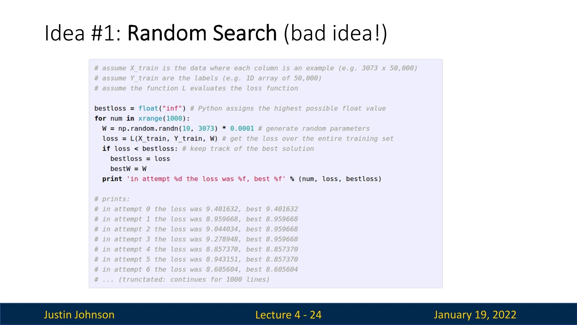
For example, as shown in Figure 4.4, random search achieves an accuracy of only \( 15.5\%\) on CIFAR-10, far from the \( 95\%\) state-of-the-art performance. The impracticality of densely sampling the parameter space motivates us to explore more intelligent strategies.

4.5.3 Optimization Idea #2: Following the Slope

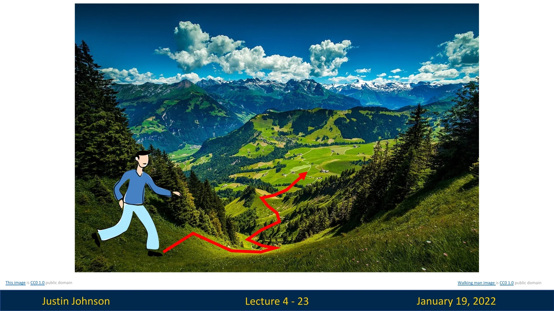
A more practical approach is to follow the slope of the loss landscape. Imagine our traveler cannot see the bottom of the valley but can feel the ground beneath his feet. By sensing the slope at his current location, he can identify the steepest downward direction and take a step in that direction.

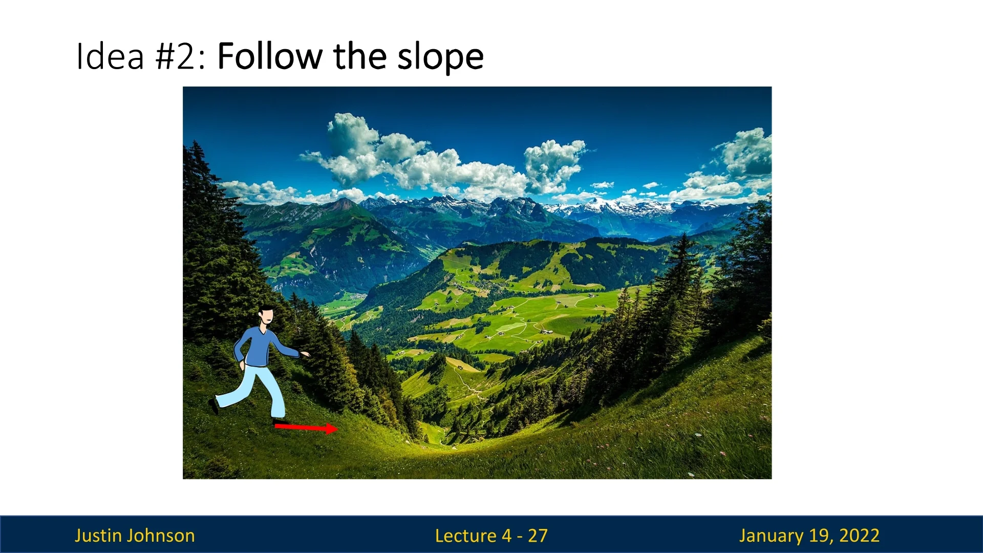
This strategy leverages local information about how the loss changes in the immediate vicinity of the current point. By iteratively stepping in the direction of steepest descent, the traveler progressively moves closer to the minimum. Despite relying solely on local information, this method is remarkably effective and forms the foundation of many optimization techniques used in machine learning.

In the following sections, we will establish the mathematical foundations for a simple yet effective method that builds upon the idea of following the slope of the loss landscape. By leveraging local information at each step in an iterative process, we aim to develop a robust approach known as gradient descent. This method will serve as a cornerstone for optimization in machine learning, guiding us toward minimizing the loss function efficiently.

4.5.4 Gradients: The Mathematical Basis

The method of steepest descent relies on the concept of gradients, a fundamental mathematical tool for analyzing changes in functions. Recall the following:

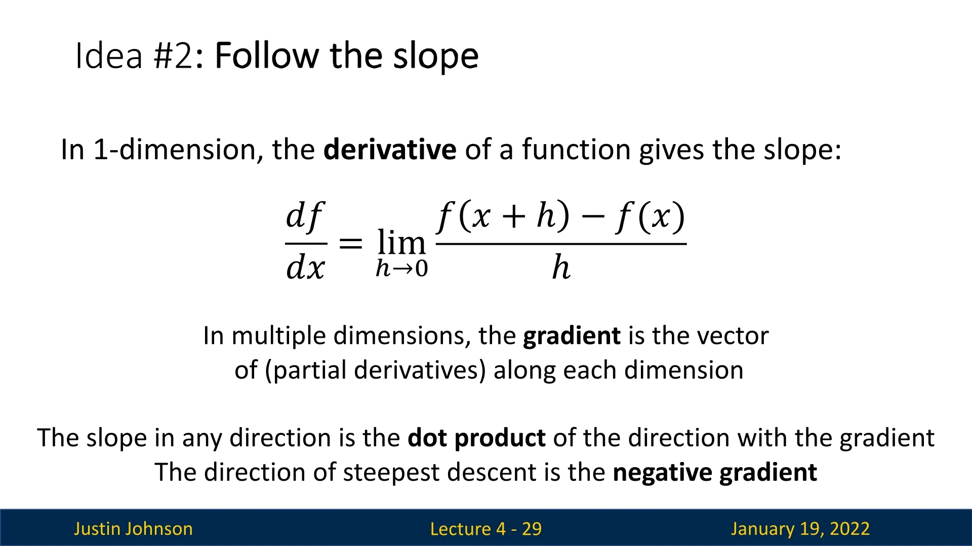
• For a scalar function \( f(x) \), the derivative \( f'(x) \) tells us how \( f(x) \) changes with a small change in \( x \). It is the slope of \( f(x) \) at any given point.
• In higher dimensions, the gradient \( \nabla f(x) \) generalizes this concept. It is a vector of partial derivatives: \[ \nabla f(x) = \begin {bmatrix} \frac {\partial f}{\partial x_1} \\ \frac {\partial f}{\partial x_2} \\ \vdots \\ \frac {\partial f}{\partial x_n} \end {bmatrix}. \] This vector points in the direction of the steepest ascent, i.e., where the function increases the fastest, and its magnitude represents the rate of this increase.

To minimize a function, we step in the opposite direction of the gradient, \( -\nabla f(x) \). This ensures the most rapid decrease in the function’s value.

Why Does the Gradient Point to the Steepest Ascent?

The gradient \( \nabla L(w) \) is the direction of the steepest ascent in the loss landscape. This can be understood as follows:

• The gradient \( \nabla L(w) \) is defined as the vector of partial derivatives of the loss \( L(w) \) with respect to each parameter in \( w \). It indicates how \( L(w) \) changes in response to small changes in \( w \).
• For any small step \( \mathbf {u} \), the change in loss can be approximated using the Taylor expansion: \[ L(w + \eta \mathbf {u}) - L(w) \approx \eta (\nabla L(w) \cdot \mathbf {u}), \] where \( \eta \) is the step size and \( \nabla L(w) \cdot \mathbf {u} \) is the dot product between the gradient and the step direction.
• The dot product is mathematically defined as: \[ \nabla L(w) \cdot \mathbf {u} = \|\nabla L(w)\| \|\mathbf {u}\| \cos (\beta ), \] where \( \beta \) is the angle between \( \nabla L(w) \) and \( \mathbf {u} \).
• The dot product \( \nabla L(w) \cdot \mathbf {u} \) is maximized when \( \cos (\beta ) = 1 \), which occurs when \( \beta = 0^\circ \) (i.e., \( \mathbf {u} \) is aligned with \( \nabla L(w) \)). This means the rate of increase in \( L(w) \) is greatest in the direction of \( \nabla L(w) \).

Thus, the gradient naturally points to the steepest ascent, where the loss increases most rapidly.

Why Does the Negative Gradient Indicate the Steepest Descent?

The steepest descent occurs in the direction opposite to the gradient, \( -\nabla L(w) \). Here’s why:

• As before, the change in loss for a small step \( \mathbf {u} \) can be approximated using the Taylor expansion: \[ L(w + \eta \mathbf {u}) - L(w) \approx \eta (\nabla L(w) \cdot \mathbf {u}), \] where \( \eta \) is the step size.
• To minimize \( L(w) \), we require: \[ \nabla L(w) \cdot \mathbf {u} < 0. \] This ensures that the new loss is smaller than the old loss.
• The dot product \( \nabla L(w) \cdot \mathbf {u} \) depends on the angle \( \beta \) between \( \nabla L(w) \) and \( \mathbf {u} \): \[ \nabla L(w) \cdot \mathbf {u} = \|\nabla L(w)\| \|\mathbf {u}\| \cos (\beta ). \] To make \( \nabla L(w) \cdot \mathbf {u} \) as negative as possible, \( \cos (\beta ) \) must equal \( -1 \), which occurs when \( \beta = 180^\circ \) (i.e., \( \mathbf {u} \) points exactly opposite to \( \nabla L(w) \)).
• Choosing \( \mathbf {u} = -\nabla L(w) \) ensures: \[ \nabla L(w) \cdot \mathbf {u} = -\|\nabla L(w)\| \|\mathbf {u}\|, \] which achieves the steepest decrease in \( L(w) \).

This property of gradients makes them indispensable for optimization. By iteratively stepping in the direction of \( -\nabla f(x) \), we can traverse high-dimensional loss landscapes efficiently and move closer to a minimum.

In the following sections, we will explore how to efficiently compute and implement gradient-based optimization methods. These techniques form the foundation of training modern machine learning models, enabling us to navigate the vast parameter spaces effectively.

4.6 From Gradient Computation to Gradient Descent

Training machine learning models involves minimizing a loss function \( L(W) \) by finding the optimal weight matrix \( W^* \). Gradient computation plays a crucial role in this process, providing the direction to adjust \( W \) to reduce the loss. This section explores two approaches to compute gradients, their limitations, and the role of gradient descent in optimization.

4.6.1 Gradient Computation Methods

Numerical Gradient: Approximating Gradients via Finite Differences

The numerical gradient approximates the gradient by perturbing each element of the weight matrix \( W \) and observing the effect on the loss. For a given element \( w_{ij} \) in \( W \), the numerical gradient is computed using the finite difference formula:

\[ \frac {\partial L}{\partial w_{ij}} \approx \frac {L(W + \Delta _{ij}) - L(W)}{ \Delta _{ij}}, \]

where \( \Delta _{ij} \) perturbs only \( w_{ij} \) by a small value \( \Delta _{ij} \) (e.g., \( \Delta _{ij} = 0.00001 \)) while leaving other elements unchanged.

Process:

• Start with an initialized weight matrix \( W \).
• For some element \( w_{ij} \), compute the perturbed loss \( L(W + \Delta _{ij}) \).
• Use the finite difference formula to calculate \( \frac {\partial L}{\partial w_{ij}} \).
• Repeat for all elements of \( W \) to approximate \( \nabla L(W) \).

Advantages:

• Easy to implement.
• Useful as a debugging tool, verifying the correctness of analytically computed gradients. For instance, PyTorch provides a built-in function (torch.autograd.gradcheck) to compare numerical and analytical gradients.

Disadvantages:

• Computational cost: Requires \( O(\mbox{#dimensions}) \) evaluations of \( L(W) \), which becomes infeasible for large models.
• Inaccuracy: Due to the finite value of \( \Delta \), the numerical gradient is an approximation, and the perturbation \( \Delta \) cannot be infinitely small as required by the gradient’s limit definition.

Analytical Gradient: Exact Gradients via Calculus

The analytical gradient computes \( \nabla L(W) \) using calculus, deriving an exact formula for the gradient based on the mathematical properties of the loss function. Unlike the numerical approach, this method is efficient and precise.

Advantages

• Exact results: Provides precise gradient values, free from numerical approximation errors.
• Computational efficiency: Scales well to high-dimensional weight matrices.

From Gradient Computation to Gradient Descent Having established how gradients can be computed, we now connect this computation to the optimization process that enables neural networks to learn from data.

Analytical vs. Numerical Computation. Both numerical and analytical approaches estimate the gradient \(\nabla L(W)\)—the rate at which the loss function \(L(W)\) changes with respect to the parameters. However, their practicality diverges dramatically at scale. Numerical gradients use finite differences, perturbing each parameter by a small amount (e.g., \(W_i \pm h\)) and measuring the corresponding change in the loss. This approach is intuitive but inefficient: for \(n\) parameters, it requires at least \(2n\) forward passes through the network, which is infeasible for models with millions of parameters.

Moreover, it is sensitive to floating-point precision and the choice of \(h\), making it unstable in high dimensions. Analytical gradients, by contrast, apply calculus directly to compute exact derivatives in a single backward pass. This method scales linearly with the number of parameters and is numerically stable, making it the only viable option for training deep networks.

Backpropagation: Computing Analytical Gradients in Practice. In deep learning, analytical gradients are not derived manually for each network architecture. Instead, they are computed automatically through the backpropagation algorithm. Backpropagation systematically applies the chain rule of calculus across the network’s computational graph, propagating error signals from the output layer backward through every intermediate operation to compute \(\nabla L(W)\). Conceptually, forward propagation computes how the parameters influence the output (the “prediction” direction), while backpropagation computes how the loss influences each parameter (the “correction” direction). Together, they form a complete learning cycle: forward pass to evaluate the model, backward pass to measure its sensitivity to change.

This combination—forward evaluation and backward differentiation—produces the exact analytical gradients required for learning, all without human derivation. We will study backpropagation and computational graphs in detail later; for now, it is enough to recognize it as the engine that turns model computations into usable gradient signals.

From Gradients to Optimization. Once gradients are available, the next step is to use them to actually minimize the loss. A gradient alone provides only local information: it tells us the steepest direction of change around the current parameters but not how far we should move or where the global minimum lies. The overarching goal is to find parameters that minimize the loss: \[ W^* = \arg \min _W L(W). \] Because deep networks involve millions of parameters and highly nonlinear loss surfaces, solving this directly in closed form is impossible. Instead, we rely on iterative optimization algorithms, most notably gradient descent, which updates parameters step by step according to: \[ W \leftarrow W - \eta \nabla L(W), \] where \(\eta > 0\) is the learning rate controlling the update magnitude.

Intuitively, backpropagation supplies the gradients—the local “slopes” of the loss surface—while gradient descent uses those slopes to guide the search for lower loss regions. If the loss landscape were a vast mountain range, backpropagation tells us which direction is downhill, and gradient descent takes one small, deliberate step in that direction. Repeating this process iteratively allows the model to descend toward a valley—ideally reaching a local or global minimum.

Together, backpropagation and gradient descent form the backbone of deep learning: one computes how to change, the other decides how to move. This interplay between gradient computation and parameter optimization is what enables neural networks to learn from data, leading naturally into the next section: Gradient Descent: The Iterative Optimization Algorithm.

4.6.2 Gradient Descent: The Iterative Optimization Algorithm

Motivation and Concept

Gradient descent is an iterative algorithm that updates \( W \) by moving in the direction of the steepest descent, guided by \( -\nabla L(W) \). The update rule is:

\[ W \gets W - \eta \nabla L(W), \]

where \( \eta \) is the learning rate, controlling the step size.

Steps of Gradient Descent

1.

Initialization: Choose a starting point \( W_0 \), often initialized randomly.

2.

Gradient Computation: Calculate \( \nabla L(W) \) analytically or numerically.

3.

Update Rule: Adjust \( W \) using the update equation.

4.

Stopping Criterion: Repeat until convergence or until a maximum number of iterations is reached.

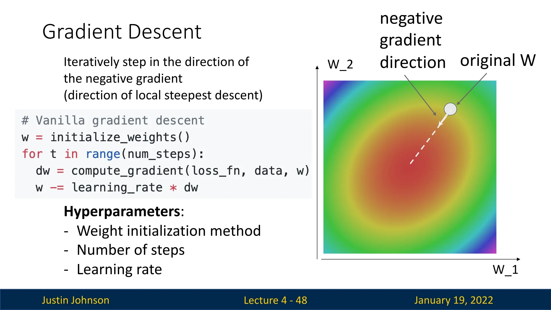
Hyperparameters of Gradient Descent

1. Learning Rate (\( \eta \))

• Controls the step size in the direction of \( -\nabla L(W) \).
• Small \( \eta \): Converges slowly.
• Large \( \eta \): Risks overshooting the minimum or diverging.

2. Weight Initialization

• The starting point \( W_0 \) significantly affects convergence.
• Random initialization is common but must ensure weights are appropriately scaled to prevent vanishing or exploding gradients.

3. Stopping Criterion

• Define when to terminate the algorithm, e.g., maximum iterations, small gradient magnitude, or minimal change in loss.

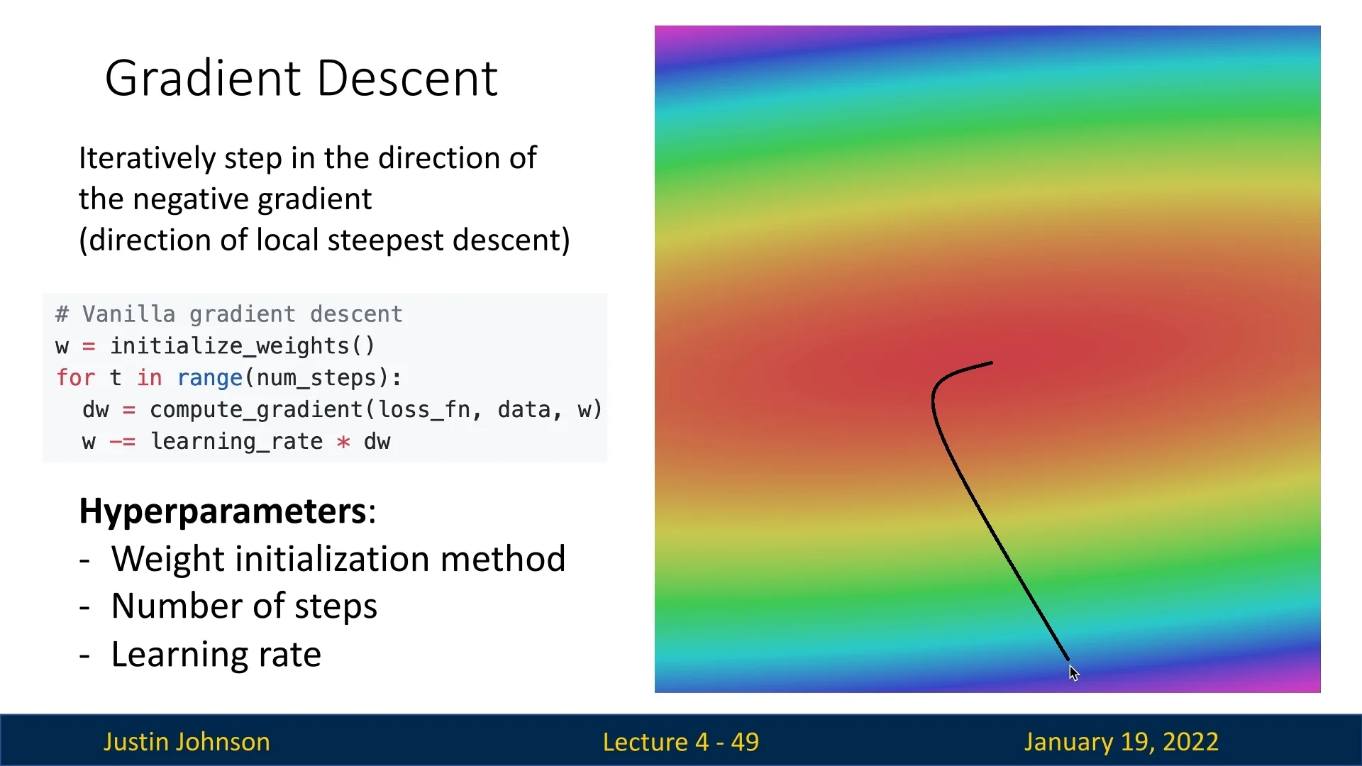
4.7 Visualizing Gradient Descent

4.7.1 Understanding Gradient Descent Through Visualization

Gradient descent can be difficult to conceptualize due to the high-dimensional nature of modern optimization problems. Since humans are limited to perceiving in three dimensions, two common visualization approaches are used to make the process more intuitive:

• 3D Surface Plot: This approach visualizes the loss landscape as a surface, where the \( x \)- and \( y \)-axes correspond to two parameters (e.g., \( \theta _0 \) and \( \theta _1 \)), and the \( z \)-axis represents the loss value. The objective is to find the combination of \( \theta _0 \) and \( \theta _1 \) that minimizes the loss, represented by the lowest point on the surface.
• 2D Contour Plot: An alternative is a 2D contour plot of the loss function, where the lines represent level sets (i.e., combinations of parameters where \( L(\theta _0, \theta _1) \) remains constant). The gradient descent process is visualized as a path that moves across these contours toward the minimum.

4.7.2 Properties of Gradient Descent

Visualization of gradient descent reveals several interesting properties of the algorithm:

Curved Trajectories Toward the Minimum

The optimization path produced by gradient descent typically follows a curved rather than straight trajectory. This behavior arises because the curvature of the loss surface—that is, how the slope changes across different directions—varies from point to point. When the curvature is anisotropic (different along different axes, as in elongated valleys), the steepest descent direction at one iteration can differ significantly from that at the next.

Since gradient descent relies solely on local gradient information, each update reorients itself according to the local slope. As the optimizer traverses regions with varying curvature, the direction of steepest descent gradually shifts, causing the overall trajectory to bend toward the minimum. In contrast, if the loss surface were perfectly isotropic (e.g., a spherical quadratic bowl), the curvature would be uniform in all directions, and the optimization path would proceed in a straight line directly toward the bottom.

Slowing Down Near the Minimum

Gradient descent starts with larger steps when the gradient magnitude is high and naturally slows down as the gradient magnitude decreases. This behavior is due to the relationship between the gradient and the steepness of the loss surface:

• The gradient is a measure of how quickly the loss function changes with respect to the parameters.
• Near the minimum of the loss surface, the loss function becomes flatter. Mathematically, this means the rate of change (i.e., the gradient) becomes smaller as we approach the minimum.

As a result:

• The magnitude of the gradient decreases in flatter regions of the loss surface, leading to smaller parameter updates during each step.
• This natural reduction in step size ensures a more refined and precise search for the optimal solution as gradient descent approaches the minimum.

By adapting to the geometry of the loss surface, gradient descent inherently balances exploration and precision, enabling effective convergence toward the minimum.

4.7.3 Why Gradient Descent Moves All Parameters Together

A tempting idea in high-dimensional optimisation is to “fix every variable but one” and march along the axes. That coordinate–descent philosophy is not what gradient methods do. Below we contrast the two approaches and explain why a single gradient step is usually preferable in machine-learning practice.

The gradient is one \( d \)-dimensional arrow For a smooth loss \( L : \mathbb {R}^{d} \to \mathbb {R} \) with parameters \( \mathbf {w} = (w_{1}, \dots , w_{d})^{\top } \), the first-order Taylor expansion reads \[ L(\mathbf {w} + \boldsymbol {\delta }) = L(\mathbf {w}) + \nabla L(\mathbf {w})^{\top } \boldsymbol {\delta } + \mathcal {O}(\|\boldsymbol {\delta }\|^{2}), \qquad \nabla L(\mathbf {w}) = \left [ \frac {\partial L}{\partial w_{1}}, \dots , \frac {\partial L}{\partial w_{d}} \right ]^{\top }. \] Among all unit-length displacements \( \boldsymbol {\delta } \), the scalar product \[ \nabla L(\mathbf {w})^{\top } \boldsymbol {\delta } = \|\nabla L(\mathbf {w})\|_{2} \cos \theta \] is maximal when \( \boldsymbol {\delta } \) is parallel to the gradient. Hence \( -\nabla L \) is the direction of steepest descent. Gradient descent therefore uses the joint update \[ \boxed {\mathbf {w} \leftarrow \mathbf {w} - \eta \nabla L(\mathbf {w})} \qquad (\eta > 0). \] Every coordinate changes in the same step; their magnitudes are scaled by the corresponding partial derivatives, but the direction is computed globally, exploiting correlations among parameters.

Axis-aligned moves may crawl or diverge Coordinate descent, in contrast, freezes \( d-1 \) variables and moves one: \[ w_{j} \leftarrow w_{j} - \eta _{j} \, \frac {\partial L}{\partial w_j}(\mathbf {w}), \qquad j = 1, \dots , d. \] Repeating this produces axis-aligned zig-zags. On the elongated quadratic \[ L(w_1, w_2) = \tfrac {1}{2} \left ( 10w_1^{2} + w_2^{2} \right ), \] gradient descent marches straight to the origin, whereas coordinate descent alternates between diminishing \( w_1 \) and \( w_2 \), wasting many iterations and possibly diverging when the individual learning rates \( \eta _j \) are poorly tuned.

Not only is coordinate descent slower, it can converge elsewhere. Because it solves a sequence of one-dimensional sub-problems, it may halt at points where each partial derivative is zero individually while the full gradient is not—a non-critical point of the original objective. In convex problems, both methods reach the global optimum eventually, but the paths—and hence practical speed—differ greatly; in non-convex landscapes they can land in distinct local minima.

When does coordinate descent shine? Axis-wise updates are attractive when:

1.

Fast conditional updates. Each 1D sub-problem has a closed form or needs only a tiny subset of the data (as in the Lasso, where one coordinate update reduces to soft thresholding).

2.

Weak parameter coupling. If the optimum of \( w_j \) barely depends on the other coordinates, a single sweep of coordinate descent can almost solve the problem.

These conditions are rare in deep learning where weights interact strongly. Gradient descent therefore uses the local geometry much more effectively.

Take-away The gradient is not merely a list of partial derivatives to apply one after another. It is a single vector giving the fastest local descent in \( \mathbb {R}^{d} \). Moving along \( -\nabla L \) exploits correlations between parameters and reaches good solutions quickly; stepping along one axis at a time ignores those correlations and usually takes a far longer—and sometimes different—route through parameter space.

4.7.4 Batch Gradient Descent

The version of gradient descent shown in Figure 4.10 is known as Batch Gradient Descent or Full Batch Gradient Descent.

In this approach:

• The loss function is computed as the average loss over the entire training set.
• The gradient at each step is computed as the sum of gradients across all training examples.

While batch gradient descent provides stable and precise updates, it becomes computationally expensive for large datasets, as each iteration requires processing the entire training set. This limitation makes it impractical for many real-world applications, where faster alternatives are needed.

4.8 Stochastic Gradient Descent (SGD)

4.8.1 Introduction to Stochastic Gradient Descent

Batch Gradient Descent, though conceptually simple, is often impractical due to its computational and memory inefficiency, especially with large datasets. A more efficient alternative is Stochastic Gradient Descent (SGD), which approximates the sum over the entire dataset (used to compute the loss and gradients) by using a minibatch of examples.

Minibatch Gradient Computation

Instead of computing gradients over the entire dataset, SGD uses minibatches:

• A minibatch is a small subset of the dataset, with common batch sizes being \(32\), \(64\), \(128\), or even larger values like \(512\) or \(1024\), depending on the available computational resources.
• The general heuristic is to maximize the batch size to fully utilize available GPU memory. For distributed training setups, minibatches can be spread across multiple GPUs or machines, allowing for very large effective batch sizes.

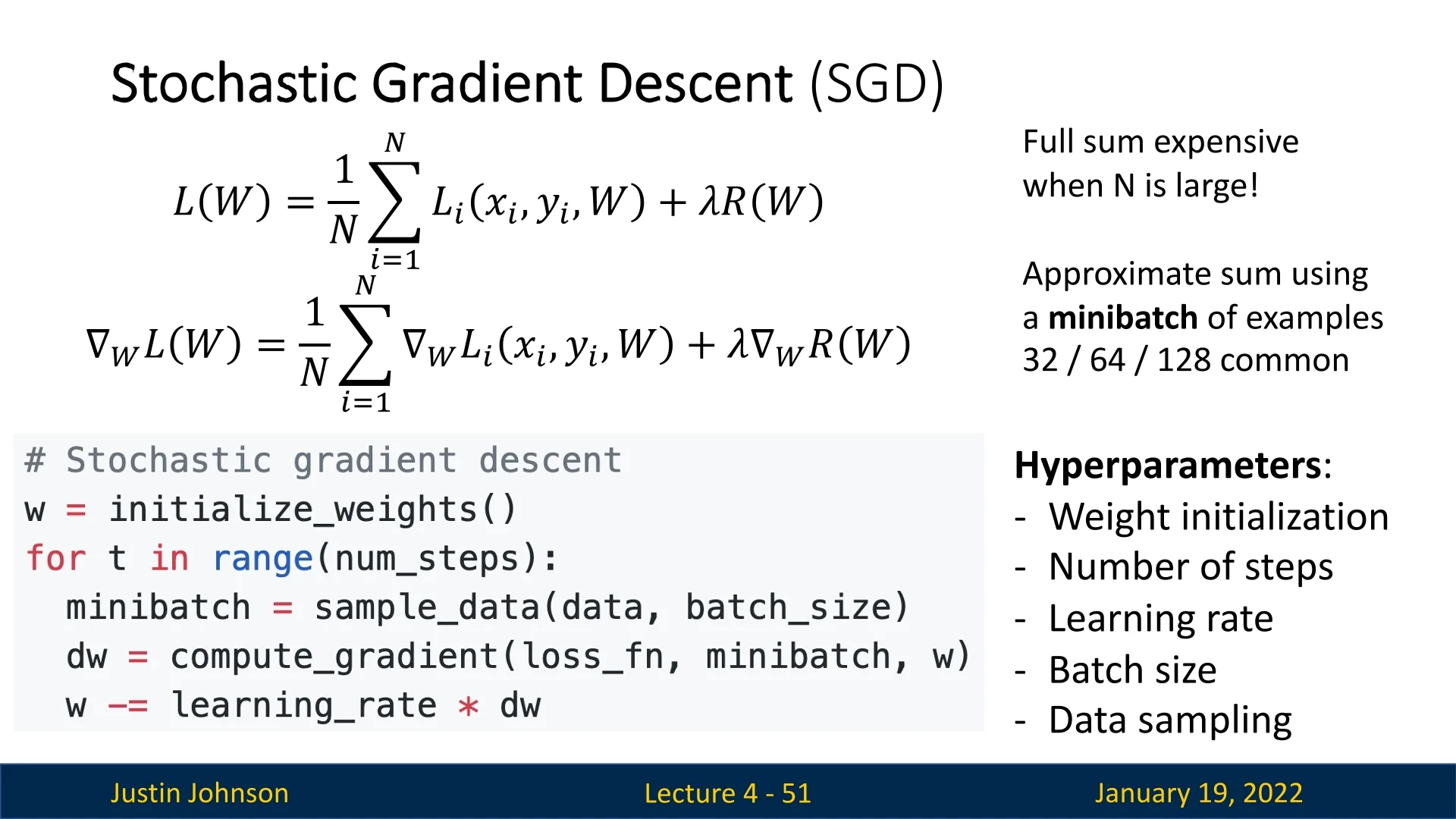
Data Sampling and Epochs

SGD introduces randomness in data selection, which affects how it iterates through the dataset:

• At the beginning of each epoch (a single pass through the entire dataset), the data is shuffled randomly to ensure varied sampling.
• During each iteration, a minibatch is selected in sequence from the shuffled data until all samples are processed, completing the epoch.
• This process is repeated for multiple epochs, with the dataset being reshuffled at the start of each one to avoid overfitting to a specific order of examples.

Why ”Stochastic”?

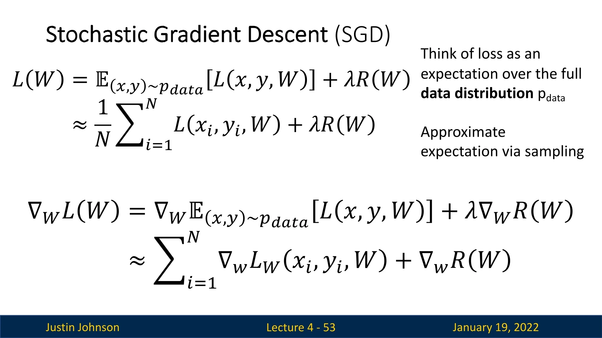
SGD is stochastic because the loss and gradient computations are based on sampled subsets of data. From a probabilistic perspective:

• The loss function can be viewed as an expectation over all possible data samples from the true underlying distribution.
• Averaging the sample loss over a minibatch approximates this expectation, and the same applies to the gradients.

4.8.2 Advantages and Challenges of SGD

Advantages

SGD provides significant computational advantages:

• Efficiency: Reduces memory requirements and computational cost per iteration.
• Scalability: Enables training on datasets too large to fit entirely into memory.

Challenges of SGD

Despite its utility, SGD comes with inherent challenges:

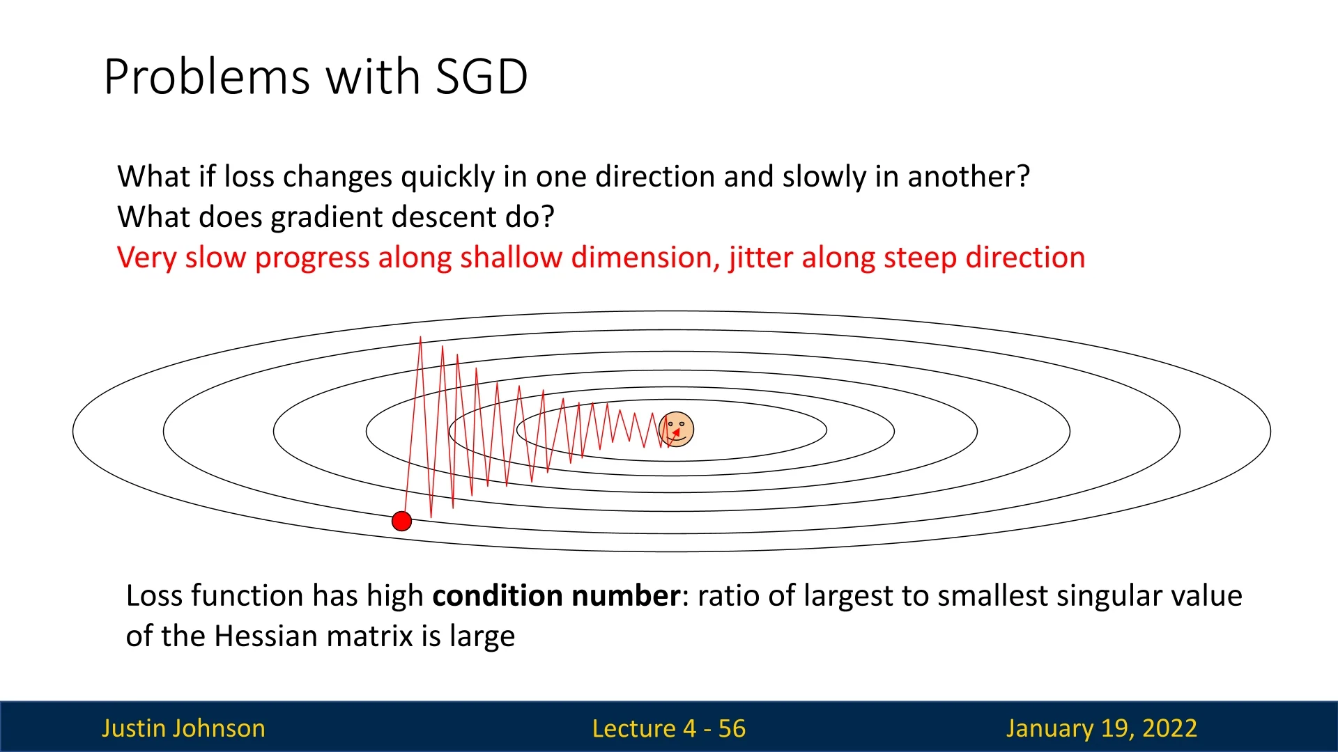
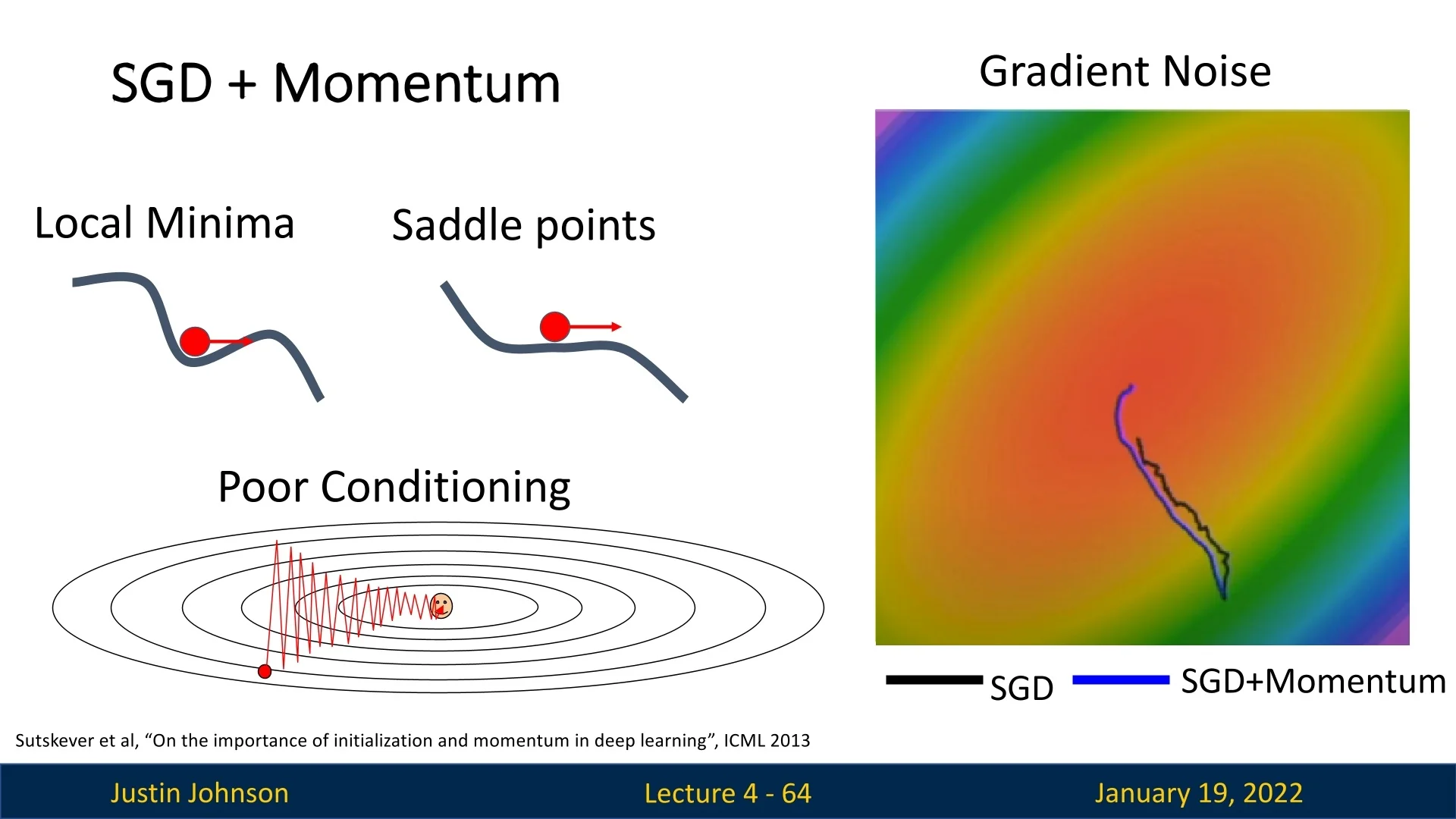
High Condition Numbers When the loss landscape changes rapidly in one direction but slowly in another, it is said to have a high condition number, which can be numerically estimated as the ratio of the largest to smallest singular values of the Hessian matrix (more about it in section 3.1. of [8]). This results in:

• Oscillations: Gradients in steep directions may overshoot the minimum, causing zig-zagging behavior.
• Slow Convergence: Reducing the step size to mitigate oscillations slows progress in shallow directions, leading to undesirable convergence times.

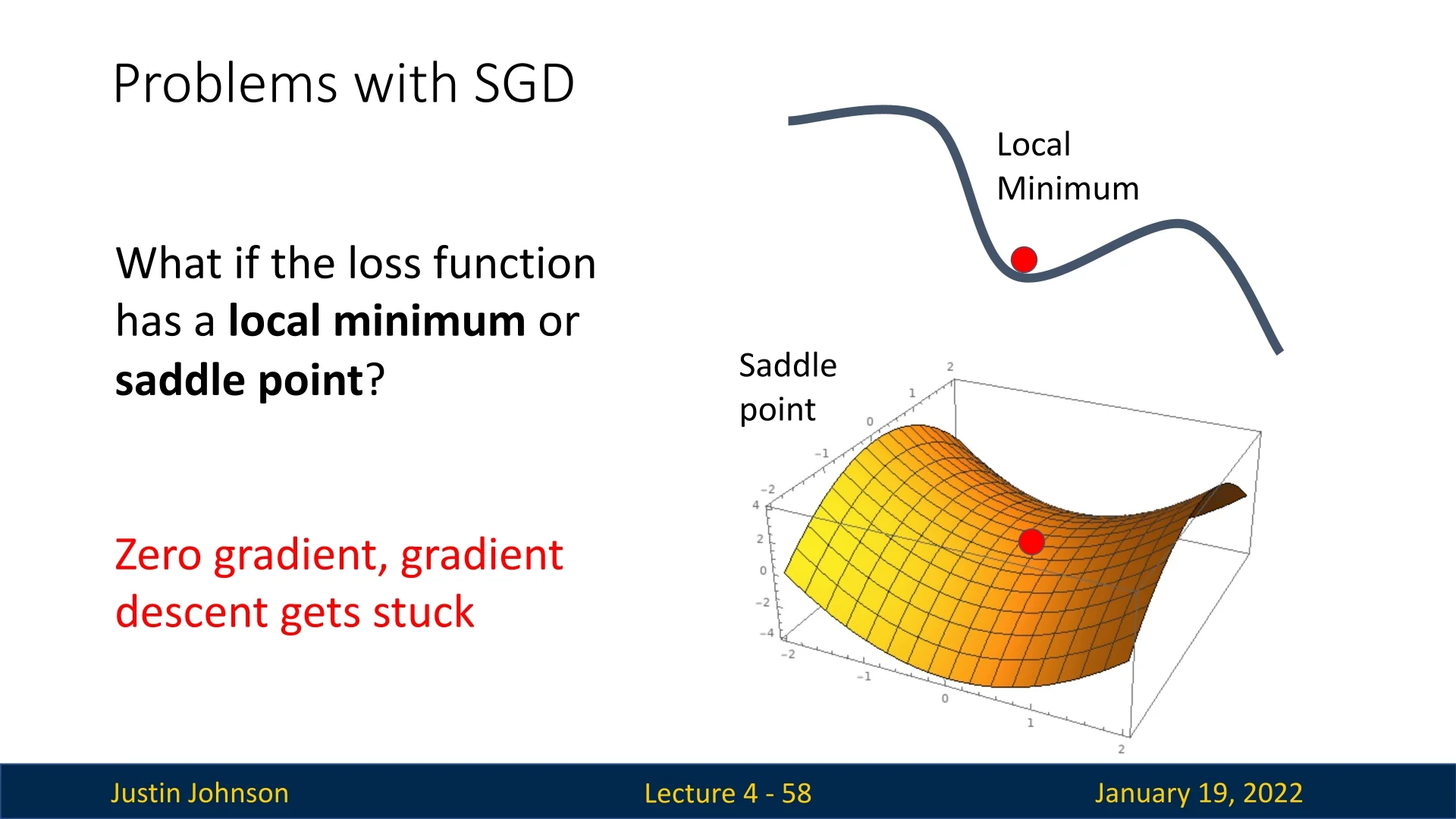
Saddle Points and Local Minima SGD may encounter:

• Saddle Points: Points where the gradient is zero, but the function increases in one direction and decreases in another. At the tip of the saddle, the gradient provides no useful direction, potentially stalling optimization.
• Local Minima: Points where the gradient is zero but are not the global minimum. The algorithm can become trapped, unable to escape without additional techniques.

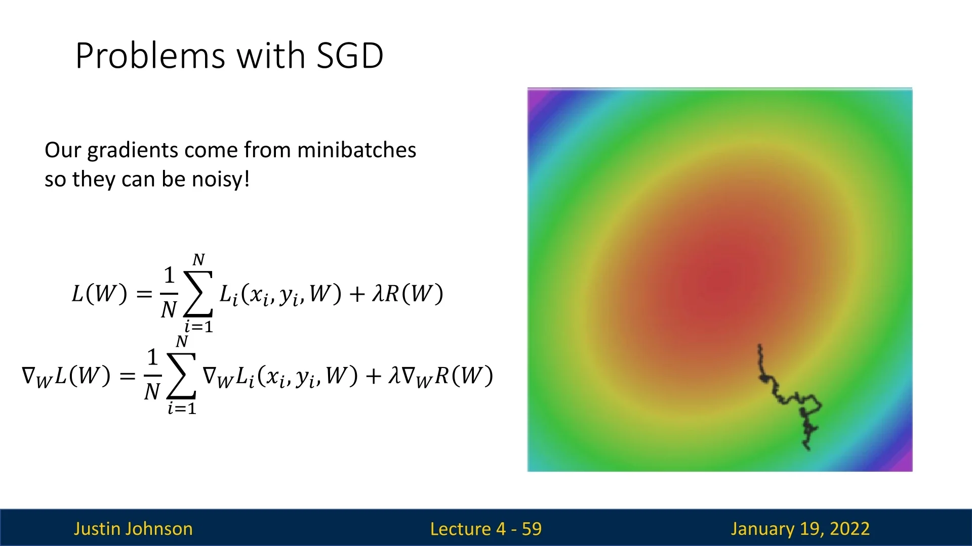
Noisy Gradients Due to the stochastic nature of SGD, gradient updates can be noisy:

• Definition of Noise: Gradients are computed from minibatches rather than the entire dataset, making them approximate and introducing randomness.
• Impact of Noise: Noisy gradients can cause the algorithm to wander around the loss surface instead of taking a direct path to the minimum, leading to slower convergence.

4.8.3 Looking Ahead: Improving SGD

While vanilla SGD is simple and effective, its limitations motivate the development of advanced variants that address its challenges. In the following sections, we will explore these modifications, starting with simpler adjustments and progressing to state-of-the-art optimizers like Adam.

4.9 SGD with Momentum

4.9.1 Motivation

While SGD is effective, it suffers from several challenges such as oscillations in ravines, difficulties escaping local minima or saddle points, and noise in gradient computations. SGD with Momentum addresses these issues by incorporating a velocity term that smooths updates and accelerates convergence in the right direction.

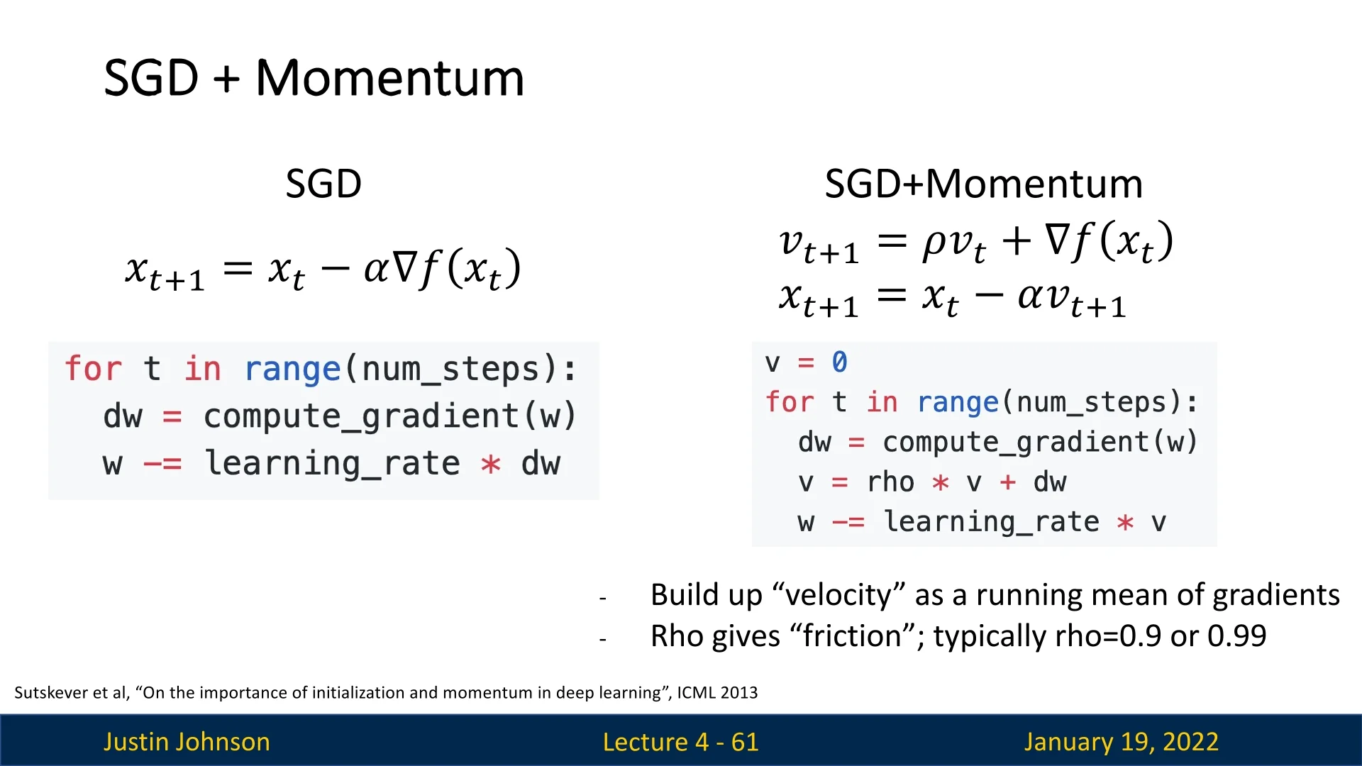
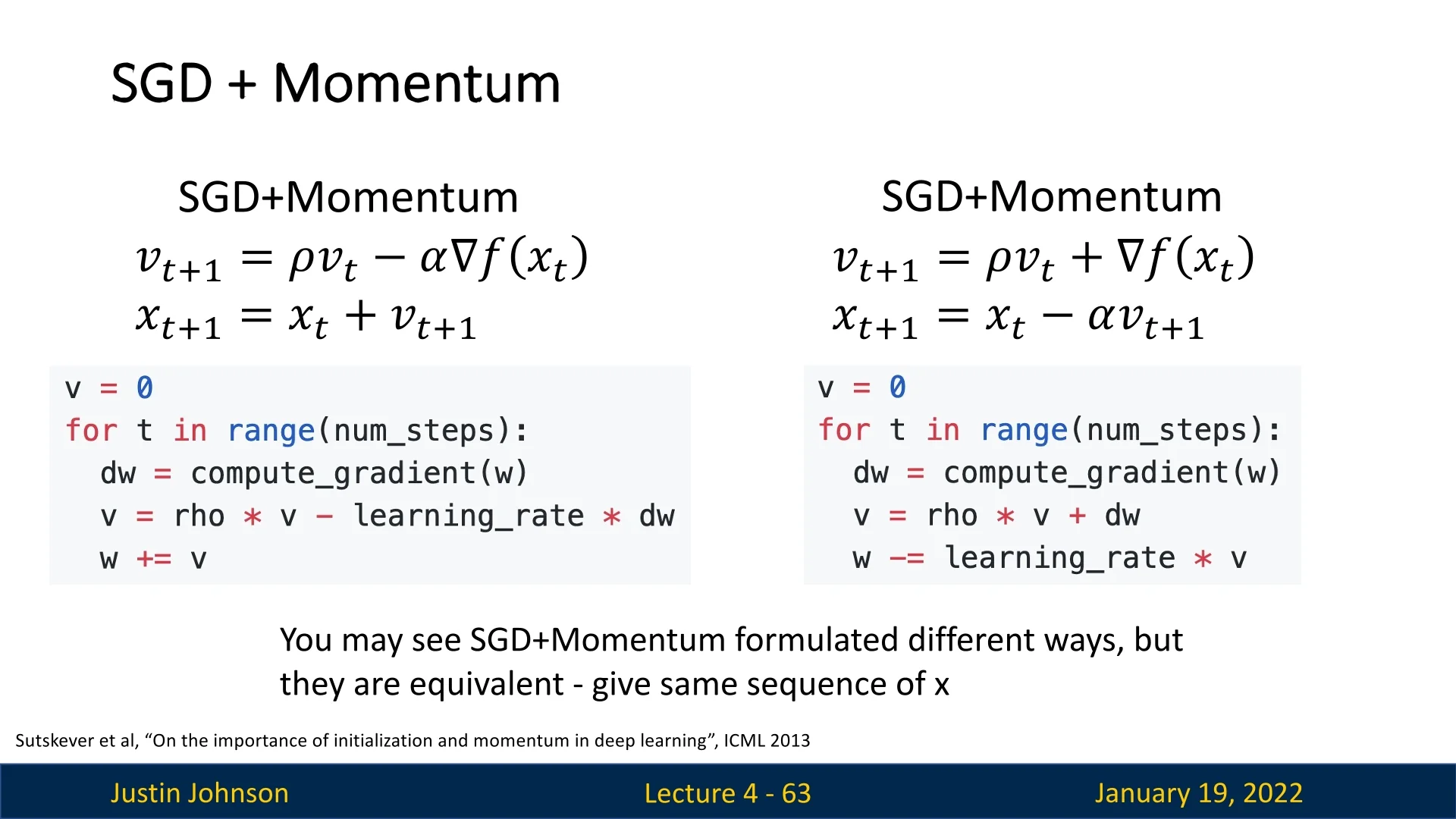
4.9.2 How SGD with Momentum Works

The concept can be visualized as a ball rolling down a high-dimensional loss surface. Instead of directly using the gradient direction for updates, we maintain a velocity vector \( \mathbf {v}_t \) that combines the current gradient and past gradients through an Exponential Moving Average (EMA).

Update Equations

At each step \( t \), we update the velocity and position as follows: \begin {align*} \mathbf {v}_t &= \rho \mathbf {v}_{t-1} + \eta \nabla L(\mathbf {x}_t), \\ \mathbf {x}_{t+1} &= \mathbf {x}_t - \mathbf {v}_t, \end {align*}

where:

• \( \rho \): Momentum coefficient, typically \( 0.9 \) or \( 0.99 \), representing the friction or decay rate. 0.9 is often the default choice, as it strikes a balance between immediate gradient and history.
• \( \eta \): Learning rate, controlling the step size.
• \( \mathbf {v}_t \): Velocity at step \( t \), an EMA of past gradients.

4.9.3 Intuition Behind Momentum

• The velocity term integrates gradients over time, effectively smoothing out noisy updates.
• The rolling-ball analogy illustrates how momentum helps maintain speed in valleys and escape saddle points or local minima.
• By decaying the velocity vector with \( \rho \), we emphasize recent gradients while retaining historical trends, allowing for smoother optimization trajectories.

Note that overall, higher momentum (e.g., 0.9 or 0.99) usually aids faster convergence and smoother updates, but can lead to overshooting or oscillations if paired with a learning rate that is too large. The larger \( \rho \), the more past gradient information is retained. Although rates like 0.99 are useful when you need to move quickly along a consistent direction, they often require careful tuning of the learning rate. Hence, 0.9 fits most tasks where consistent gradient directions exist. Larger values will be used only for deep models with large datasets, in which gradients are relatively stable.

4.9.4 Benefits of Momentum

Momentum addresses the three key problems of SGD:

• Local Minima and Saddle Points: The velocity term allows the optimizer to pass through these points due to accumulated momentum.
• Poor Conditioning: Oscillations in ravines are smoothed, and updates are more stable as momentum averages out noisy gradients.
• Noisy Gradients: Momentum helps filter out random fluctuations in gradient directions, resulting in a more direct path to the minimum.

4.9.5 Downsides of Momentum

Despite its advantages, SGD with Momentum has several limitations:

• Hyperparameter Sensitivity: The choice of \( \rho \) (momentum coefficient) and \( \eta \) (learning rate) significantly affects performance.
• Memory Requirements: Additional storage is needed to maintain velocity vectors for all parameters.
• Lack of Adaptivity: Momentum does not adapt the learning rate for individual weights, limiting its effectiveness for sparse gradients or features with varying importance.
• Robustness: Momentum can amplify noise under certain conditions, leading to erratic updates.
• Slower Convergence: Advanced optimizers like Adam often achieve faster convergence rates.

4.9.6 Nesterov Momentum: A Look-Ahead Strategy

Overview

Nesterov Momentum builds upon SGD with Momentum by introducing a ”look-ahead” mechanism. Instead of calculating the gradient at the current position, Nesterov computes it at the projected future position, determined by the current velocity vector. This adjustment allows for more precise updates and improved convergence behavior.

Mathematical Formulation

The Nesterov update rules are given as: \begin {align*} \mathbf {v}_{t+1} &= \rho \mathbf {v}_t - \eta \nabla f\big (\mathbf {x}_t + \rho \mathbf {v}_t\big ), \\ \mathbf {x}_{t+1} &= \mathbf {x}_t + \mathbf {v}_{t+1}, \end {align*}

where:

• \( \rho \): Momentum coefficient, controlling the influence of past velocities.
• \( \eta \): Learning rate.
• \( \nabla f\big (\mathbf {x}_t + \rho \mathbf {v}_t\big ) \): Gradient computed at the ”look-ahead” position.

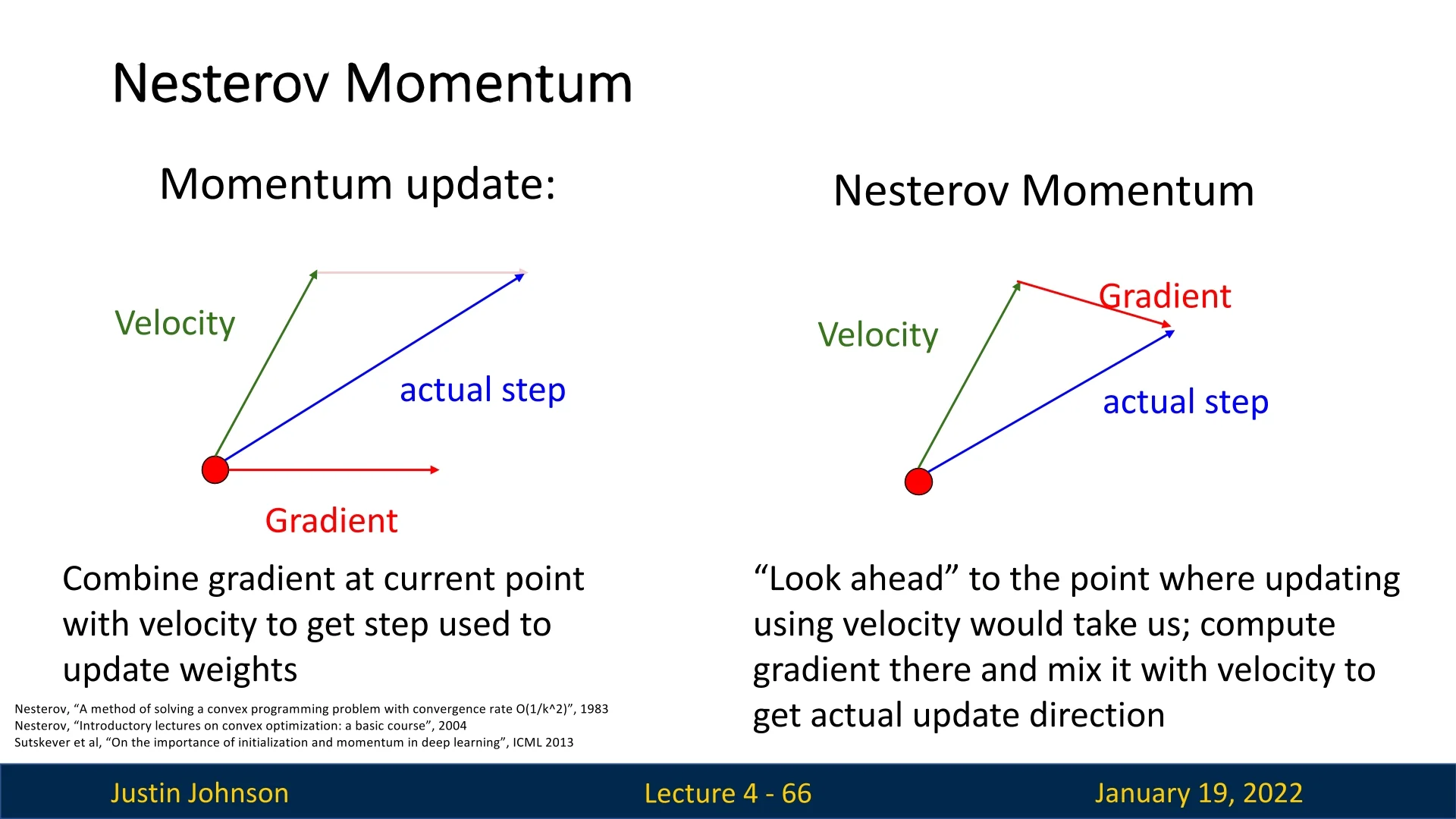
Motivation and Advantages

Nesterov Momentum improves upon traditional momentum methods by providing a more precise update mechanism, leading to faster convergence and reduced oscillations. The key motivations and advantages include:

• Reduced Oscillations:

  • In traditional momentum methods, the gradient is computed at the current position, and the accumulated velocity can overshoot the minimum due to excessive momentum, especially in steep directions.
  • Nesterov Momentum addresses this by computing the gradient at a ”look-ahead” position (\( \mathbf {x}_t + \rho \mathbf {v}_t \)), effectively anticipating the overshoot and applying a correction before the step is taken.
  • By integrating this ”look-ahead gradient”, Nesterov smoothens the update trajectory, particularly in ravines (areas with steep gradients in one direction and shallow gradients in another), thereby reducing zig-zagging behavior.

• Faster Convergence:

  • The look-ahead mechanism allows Nesterov Momentum to make more informed updates, as the gradient incorporates information about where the optimizer is heading, not just where it currently is.
  • This results in more efficient use of gradient information, leading to quicker progress along flat regions and better handling of curved loss landscapes.
  • Faster convergence also stems from the smaller step adjustments needed to compensate for overshooting, ensuring that the optimizer focuses on approaching the minimum directly.

• Improved Stability in High-Condition-Number Landscapes:

  • In poorly conditioned loss surfaces, where gradients change drastically along different directions, the look-ahead gradient reduces oscillations in the steep direction while maintaining steady progress in the shallow direction.
  • This makes Nesterov particularly effective in minimizing the effect of uneven gradient magnitudes across dimensions, stabilizing the optimization process.

Reformulation for Practical Implementation

From the “lookahead” definition to a one–gradient update The classical Nesterov accelerated gradient (NAG) formulation “looks ahead” before measuring the slope: \[ \underbrace {\mathbf {y}_t}_{\mbox{lookahead}} = \mathbf {x}_t + \rho \,\mathbf {v}_t, \quad \mathbf {v}_{t+1} = \rho \,\mathbf {v}_t - \eta \,\nabla f(\mathbf {y}_t), \quad \mathbf {x}_{t+1} = \mathbf {x}_t + \mathbf {v}_{t+1}. \tag {NAG} \label {eq:chapter4_nag_lookahead} \] This version depends on the gradient evaluated at the projected (lookahead) point \(\mathbf {y}_t\). While elegant in theory, it poses practical challenges in modern automatic differentiation frameworks: it requires either a second forward–backward computation at \(\mathbf {y}_t\) or reparameterizing the model to temporarily evaluate the gradient there.

A practical, one–backward-pass reformulation. To avoid this inefficiency, most modern deep learning libraries adopt an algebraically equivalent (up to first-order accuracy) form that requires only a single gradient evaluation at the current parameters \(\mathbf {x}_t\): \begin {equation} \boxed { \begin {aligned} \mathbf {v}_{t+1} &= \rho \,\mathbf {v}_t - \eta \,\nabla f(\mathbf {x}_t),\\ \mathbf {x}_{t+1} &= \mathbf {x}_t + \rho \,\mathbf {v}_{t+1} - \eta \,\nabla f(\mathbf {x}_t) \end {aligned}} \tag {NAG-prac} \label {eq:chapter4_nag_practical} \end {equation} This form preserves Nesterov’s anticipatory effect while using only one backward pass per iteration, making it efficient and fully compatible with standard autodiff frameworks.

Why this works (step by step) Starting from the lookahead formulation ([ref]), expand the update for \(\mathbf {x}_{t+1}\): \[ \mathbf {x}_{t+1} = \mathbf {x}_t + \rho \,\mathbf {v}_t - \eta \,\nabla f(\mathbf {x}_t + \rho \,\mathbf {v}_t). \] Using a first-order Taylor approximation of the gradient around \(\mathbf {x}_t\): \[ \nabla f(\mathbf {x}_t + \rho \,\mathbf {v}_t) \approx \nabla f(\mathbf {x}_t) + \underbrace {\nabla ^2 f(\mathbf {x}_t)}_{H_t}\,(\rho \,\mathbf {v}_t), \] and substituting gives: \[ \begin {aligned} \mathbf {v}_{t+1} &\approx \rho \,\mathbf {v}_t - \eta \,\nabla f(\mathbf {x}_t) - \eta \,\rho \,H_t\mathbf {v}_t,\\ \mathbf {x}_{t+1} &\approx \mathbf {x}_t + \rho \,\mathbf {v}_t - \eta \,\nabla f(\mathbf {x}_t) - \eta \,\rho \,H_t\mathbf {v}_t. \end {aligned} \] Neglecting the second-order curvature term \(-\eta \,\rho \,H_t\mathbf {v}_t\)—which is small for typical step sizes and vanishes for quadratic objectives—yields precisely the single-gradient form (4.1). Thus, the practical reformulation is accurate up to \(\mathcal {O}(\eta \rho )\) curvature effects and exact for quadratic loss functions.

Equivalent “library style” formulation Deep learning frameworks (e.g., PyTorch, TensorFlow) commonly express Nesterov momentum in the following algebraically identical update: \[ \mathbf {g}_t = \nabla f(\mathbf {x}_t), \qquad \mathbf {v}_{t+1} = \rho \,\mathbf {v}_t + \mathbf {g}_t, \qquad \mathbf {d}_t = \mathbf {g}_t + \rho \,\mathbf {v}_{t+1}, \qquad \mathbf {x}_{t+1} = \mathbf {x}_t - \eta \,\mathbf {d}_t. \] Substituting \(\mathbf {d}_t\) recovers the same parameter displacement as in (4.1), confirming that both forms are equivalent up to first order. This implementation performs one gradient computation per iteration and avoids explicit “lookahead” states.

Why this reformulation is preferred in practice

• Single backward pass. Autodiff frameworks naturally provide \(\nabla f(\mathbf {x}_t)\). Computing at \(\mathbf {y}_t\) would require an extra graph traversal or redundant backward pass.

• Preserved acceleration effect. Despite dropping the explicit lookahead gradient, the update still “anticipates” future motion through the momentum term \(\rho \,\mathbf {v}\), maintaining Nesterov’s key speedup.

• Controlled approximation. The deviation from the exact formulation is of second order in \(\eta \) and \(\rho \), negligible for practical step sizes. Empirically, both variants yield nearly identical convergence curves while the practical version is faster and simpler to implement.

Take-away Nesterov’s central insight—evaluate the gradient ahead of the current point to anticipate future motion—can be implemented efficiently with a single gradient at the current iterate. The resulting practical update (4.1) preserves the intended acceleration behavior while integrating seamlessly into modern deep learning optimizers that rely on one forward–backward pass per iteration.

Comparison with SGD and SGD+Momentum

Momentum-based methods, including Nesterov, tend to overshoot near minima due to accumulated velocity. Nesterov’s look-ahead mechanism mitigates this overshooting, producing a more efficient path to the minimum.

Limitations of Nesterov Momentum and the Need for Adaptivity

While Nesterov Momentum addresses several shortcomings of traditional momentum methods, it still has limitations that motivate further advancements in optimization techniques:

• Uniform Learning Rate:

  • Nesterov Momentum uses a single global learning rate for all weight components, regardless of their individual gradient behavior.

  • In scenarios where gradients vary significantly across dimensions (e.g., high-condition-number landscapes or sparse features), this uniform learning rate can lead to inefficient updates:

    • Large gradients may result in overly cautious updates, slowing down convergence.
    • Small gradients may cause under-updated weights, making progress in flat regions painfully slow.

• Sensitivity to Hyperparameters:

  • Nesterov Momentum requires careful tuning of both the learning rate (\( \eta \)) and the momentum parameter (\( \rho \)).
  • Suboptimal hyperparameter settings can lead to erratic behavior, such as oscillations, overshooting, or excessively slow convergence.

• No Adaptivity to Gradient Magnitudes:

  • Nesterov Momentum does not adapt the learning rate based on the magnitude of the gradients. This is particularly problematic for sparse data or infrequent features, where gradients may carry highly informative yet small signals.
  • The lack of adaptivity can hinder optimization in modern machine learning applications, such as natural language processing or deep learning for image recognition, where gradient magnitudes can vary significantly.

• Stochastic Noise Amplification:

  • While Nesterov reduces oscillations, its velocity updates can amplify noise in stochastic gradients, leading to suboptimal parameter updates and slower convergence.
  • This issue becomes particularly evident in noisy or sparse datasets, where gradient signals are less stable.

Motivation for a Better Optimizer: AdaGrad To overcome these limitations, we seek optimizers that:

• Adjust learning rates adaptively for each parameter based on the historical behavior of its gradients.
• Mitigate the impact of high-condition-number landscapes by dampening updates in steep directions while accelerating progress in flat regions.
• Improve handling of sparse data and infrequent features by increasing learning rates for weights with smaller gradients.

AdaGrad introduces an adaptive learning rate mechanism that addresses these issues by scaling updates inversely proportional to the square root of the accumulated squared gradients. This adaptivity enables AdaGrad to make more efficient and stable progress across diverse optimization landscapes, as we will explore in the next section.

4.10 AdaGrad: Adaptive Gradient Algorithm

AdaGrad, short for Adaptive Gradient Algorithm, adjusts the learning rate for each parameter based on the historical squared gradients. This adaptivity allows the optimizer to handle scenarios where different parameters require significantly different learning rates.

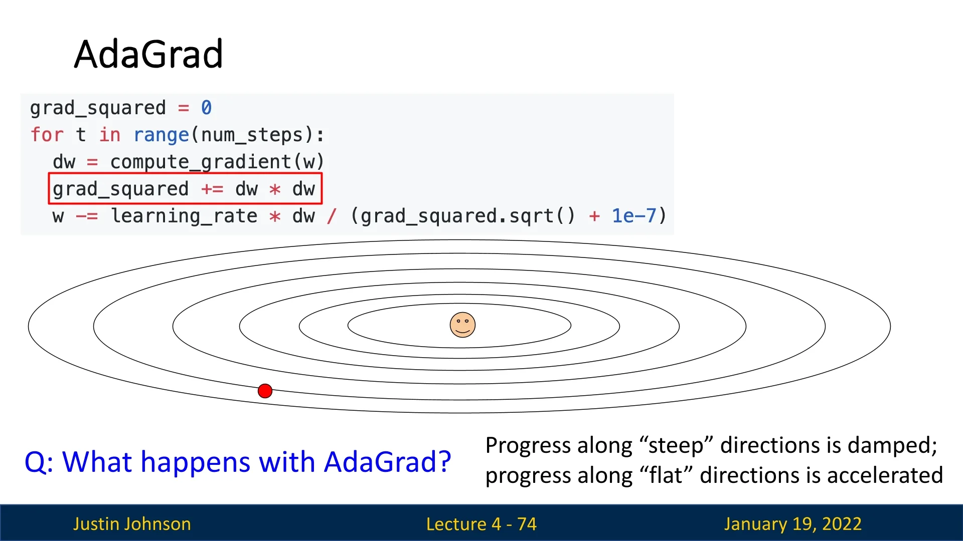
4.10.1 How AdaGrad Works

Rather than using a fixed global learning rate \( \eta \), AdaGrad adjusts the learning rate for each parameter \( w_i \) dynamically. We denote the parameters (weight components) as: \(w=\left (w_0, w_1 \cdots w_i, \cdots , w_n\right )\), and at step t as: \(w_t=\left (w_{t_0}, w_{t_1} \cdots w_{t_i}, \cdots , w_{t_n}\right )\) We denote the gradient of the loss with respect to each weight component at step t as \(g_{t_i}=\nabla _w J\left (w_{t_i}\right )\).

Updating the Weight Matrix Components Unlike SGD in which the update for each parameter (weight component) at step \(t\) is: \[ w_{t_{i+1}}=w_{t_i}-\eta \cdot g_{t_i} \] In Adagrad the update rule for each parameter (weight component) at step \(t\) is \[ w_{t_{i+1}}=w_{t_i}-\frac {\eta }{\sqrt {G_{t_{(i, i)}}+\epsilon }} \cdot g_{t_i} \] \(G_t \in \mathbb {R}^{n \times n}\) is a diagonal matrix, where each diagonal element \((i, i)\) is the sum of squares of the gradients with respect to \(w_i\) at the step, meaning, \(G_{t_{(i, i)}}=\sum _{j=0}^t\left (g_{j_{i},}\right )^2\). Also note that \(\epsilon \) serves as a smoothing term, that helps to avoid division by 0 (usually in the form of \(1 e-8\) ).

As \(G_t \in \mathbb {R}^{n \times n}\) has the sum of squares of all past gradients with respect to all parameters \(w\) along its diagonal, We can vectorize our implementation by performing a matrix-vector product \(\odot \) between \(G_t\) and \(g_t\): \[ w_{t}=w_{t-1}-\frac {\eta }{\sqrt {G_{t}+\epsilon }} \cdot g_{t} \]

Why Does This Work? The division by \( \sqrt {G_t + \epsilon } \) achieves two things:

• Damping Large Gradients: Parameters with consistently large gradients will accumulate larger \( G_t[i] \) values, reducing their effective learning rate. This dampens oscillations in steep regions of the loss surface.
• Accelerating Small Gradients: Parameters with small or infrequent gradients will have smaller \( G_t[i] \) values, increasing their effective learning rate. This ensures progress in flatter regions or for parameters with sparse updates.

4.10.2 Advantages of AdaGrad

• Adaptive Learning Rates:

  • No need for manual tuning of \( \eta \), as the learning rate is adjusted dynamically for each parameter.

• Effective for Sparse Gradients:

  • Particularly useful in scenarios like natural language processing or recommendation systems, where certain features or gradients are updated infrequently.

4.10.3 Disadvantages of AdaGrad

Despite its strengths, AdaGrad has notable limitations:

• Aggressive Learning Rate Decay:

  • The cumulative sum of squared gradients \( G_t[i] \) grows over time, causing the learning rate to shrink excessively. This often leads to slow convergence or stagnation, particularly in non-convex optimization problems.

• No Momentum:

  • AdaGrad does not include a momentum term to smooth out oscillations or accelerate convergence along shallower dimensions.

• Inability to Forget Past Gradients:

  • All past gradients are treated equally, which can be problematic in non-convex problems with varying loss landscape dynamics. An example to emphasize how big of an issue this is: we might be going down a steep slope, then reaching a plateau, and then a steep portion again, and the fact that our \(G_t\) got really big and our updates, in turn, get really small, will make our optimization efforts ineffective.

4.11 RMSProp: Root Mean Square Propagation

4.11.1 Motivation for RMSProp

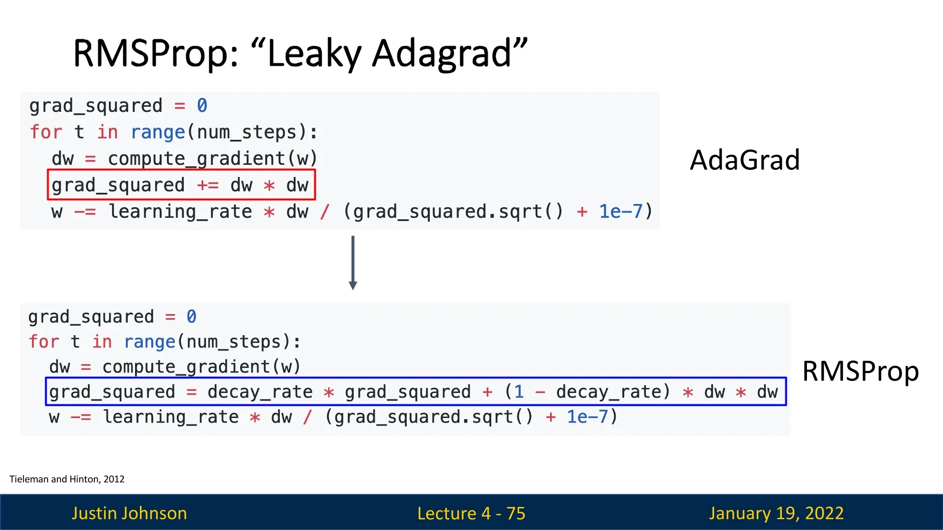
While AdaGrad effectively adapts learning rates for individual parameters by accumulating squared gradients, it suffers from a major limitation: the accumulation grows indefinitely. Over time, this causes the effective learning rate to shrink excessively, slowing down optimization or halting it entirely.

RMSProp addresses this issue by introducing a decay factor, which transforms AdaGrad into a leaky version of itself. By ensuring that only recent gradients significantly influence the updates, RMSProp prevents the learning rate from diminishing too aggressively, allowing optimization to maintain steady progress over time.

4.11.2 How RMSProp Works

RMSProp modifies the sum of squared gradients \( G_t \) in AdaGrad to an exponentially weighted moving average (EWMA) of squared gradients: \[ G_t = \rho G_{t-1} + (1 - \rho ) g_t^2, \] where:

• \( G_t \): The EWMA of squared gradients at step \( t \),
• \( \rho \): The decay rate (forgetting factor, typically set to 0.9),
• \( g_t^2 \): The element-wise square of the gradient at step \( t \).

Using this updated \( G_t \), the parameter update rule becomes: \[ w_{t+1} = w_t - \frac {\eta }{\sqrt {G_t + \epsilon }} \cdot g_t, \] where:

• \( \eta \): The learning rate,
• \( \epsilon \): A small constant (e.g., \( 10^{-8} \)) to prevent division by zero.

4.11.3 Updating the Weight Matrix Components

We denote:

• Parameters (weight components): \( w = [w_1, w_2, \ldots , w_n] \),
• Gradient of the loss with respect to each parameter at step \( t \): \( g_{t_i} = \nabla _w J(w_{t_i}) \).

The update for each parameter \( w_i \) is: \[ G_t[i] = \rho G_{t-1}[i] + (1 - \rho ) g_t[i]^2, \] \[ w_{t+1}[i] = w_t[i] - \frac {\eta }{\sqrt {G_t[i] + \epsilon }} \cdot g_t[i]. \]

This ensures parameters with consistently large gradients have reduced learning rates, while parameters with smaller gradients have relatively larger learning rates.

4.11.4 Advantages of RMSProp

• Prevents Learning Rate Decay:

  • By introducing a forgetting factor, RMSProp avoids the excessive shrinking of learning rates observed in AdaGrad.

• Adaptability:

  • RMSProp adjusts learning rates dynamically based on the history of squared gradients, making it suitable for non-convex problems.

• Stability:

  • By dampening progress along steep directions, RMSProp reduces oscillations while accelerating motion in flatter regions.

4.11.5 Downsides of RMSProp

No Momentum Carry-Over

While RMSProp adapts its learning rate per parameter, it does not explicitly maintain a “velocity” term that accumulates gradients over time.

• Reduced Acceleration: In standard momentum-based methods (e.g., SGD with momentum), a portion of the previous update carries over to the next, helping the optimizer power through saddle points and shallow minima. RMSProp does not have this explicit accumulation, but despite that, it (and other adaptive optimizers like Adagrad) is not powerless against saddle points or local minima. By adjusting step sizes dimension-wise, RMSProp can still navigate tricky landscapes—sometimes more effectively than vanilla SGD. However, without an explicit momentum mechanism, it may need more careful tuning (sensitivity to hyperparameters) or additional iterations to escape challenging regions.

Bias in Early Updates

RMSProp maintains exponentially decaying running averages of squared gradients: \[ G_t = \rho G_{t-1} + (1 - \rho )\,g_t^2, \] where \(\rho \) (\(0 < \rho < 1\)) is the decay factor, and the model parameters \(w\) are updated as: \[ w_{t+1} \;\leftarrow \; w_{t} \;-\; \eta \,\frac {g_t}{\sqrt {G_t + \epsilon }}, \] with \(\eta \) being the learning rate and \(\epsilon \) a small constant for numerical stability.

• Underestimated Variances Lead to Larger Steps: Early in training, \(G_t\) can be underestimated due to insufficient historical data. This makes the denominator, \(\sqrt {G_t + \epsilon }\), smaller than it should be, which can produce updates larger than intended and potentially lead to instability or overshooting.
• No Built-In Bias Correction: Unlike Adam, RMSProp does not include a bias-correction mechanism to compensate for these underestimated running averages in the initial training phase.

Sensitivity to Hyperparameters

RMSProp requires two main hyperparameters:

• Decay Factor (\(\rho \)): Determines how quickly the running average of the squared gradients decays.

  • A large \(\rho \) (close to 1) makes the exponential average change more slowly, placing greater emphasis on older gradient information.
  • A smaller \(\rho \) places more weight on recent gradients, allowing faster adaptation to new changes in the loss landscape.
• Learning Rate (\(\eta \)): Controls the scale of each update. Poor choices can cause exploding or vanishing updates, depending on the curvature of the loss landscape.

Because both \(\rho \) and \(\eta \) must be tuned, RMSProp can be quite sensitive to hyperparameter selection.

4.11.6 Motivation for Adam, a SOTA Optimizer

Adam (Adaptive Moment Estimation) extends RMSProp in several key ways:

• Incorporates Momentum: Adam adds an explicit exponential moving average of the gradients, giving it a “velocity”-like term that smooths updates and helps traverse saddle points more effectively.
• Bias Correction: Adam corrects for the initially underestimated moving averages, preventing steps from becoming excessively large at the start of training.
• Robust Defaults: Adam’s standard hyperparameters (\(\beta _1 = 0.9\), \(\beta _2 = 0.999\), \(\eta = 1e-3 \mbox{ or } 1e-4 \) for the learning rate) are often effective across many tasks, easing the tuning burden compared to vanilla RMSProp.

By blending momentum, adaptive learning rates, and bias correction, Adam often converges more smoothly and quickly than pure RMSProp, while retaining many of RMSProp’s advantages in complex, high-dimensional optimization landscapes.

4.12 Adam: Adaptive Moment Estimation

4.12.1 Motivation for Adam

Adam combines the strengths of momentum-based methods (like SGD+Momentum) and adaptive learning rate methods (like RMSProp). By integrating these two techniques, Adam effectively handles optimization challenges such as:

• Escaping saddle points and overcoming noisy gradients.
• Reducing sensitivity to hyperparameter tuning.
• Achieving faster and more stable convergence, even on complex, non-convex loss landscapes.

The name Adam stands for Adaptive Moment Estimation, referring to its use of first and second moments of gradients:

• The first moment represents the mean of gradients, which estimates the rate of change of the model parameters.
• The second moment represents the variance of gradients, reflecting how spread out the gradients are around the mean value.

By utilizing these moments, Adam provides better control over optimization, leveraging the gradient’s direction and its historical updates for efficient learning.

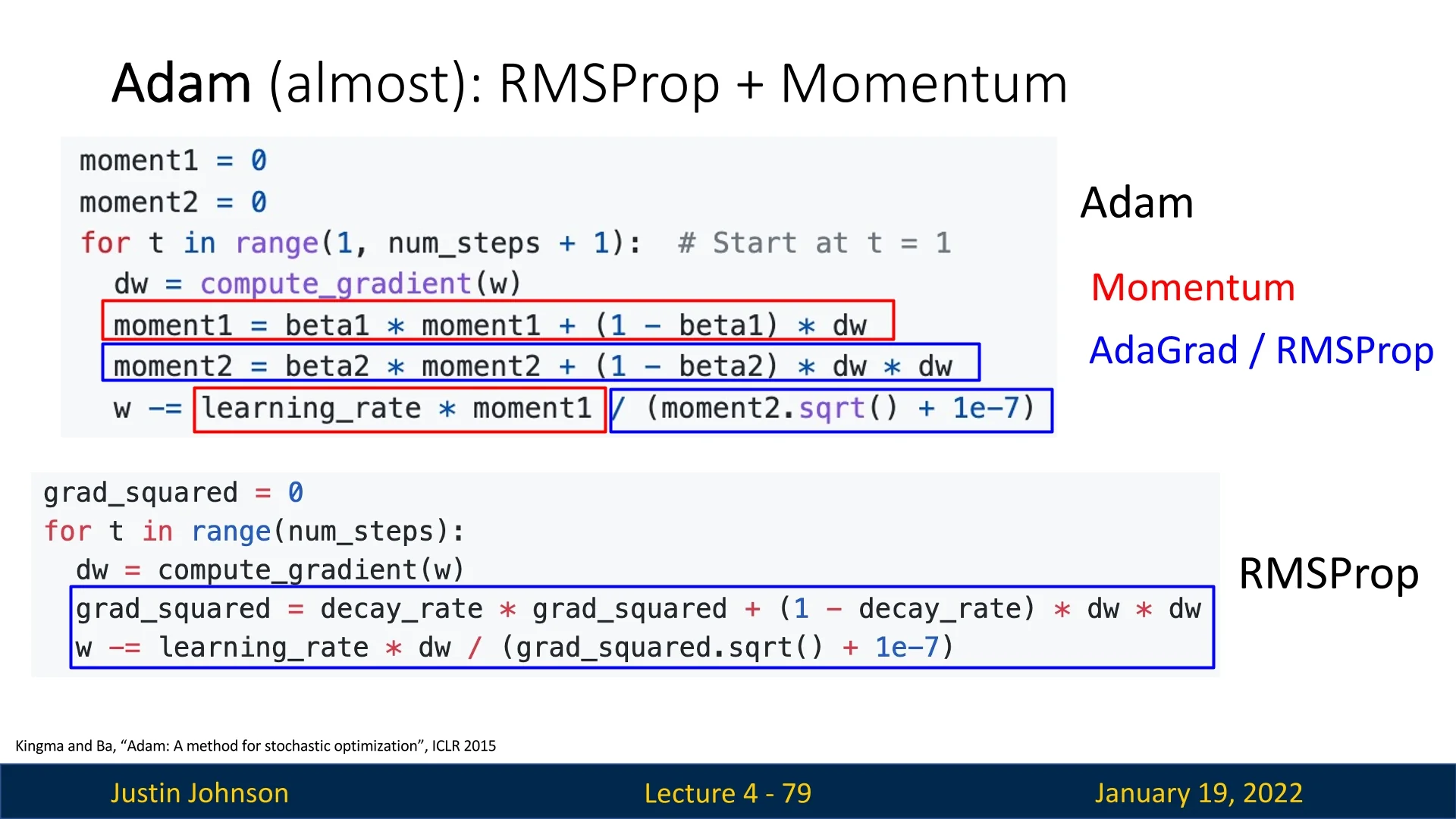
4.12.2 How Adam Works

Adam maintains two moving averages during training:

• First moment (mean): An exponentially weighted average of the gradients, capturing their direction and magnitude over time.
• Second moment (variance): An exponentially weighted average of squared gradients, scaling updates based on their historical magnitudes.

The update equations are: \[ m_t = \beta _1 m_{t-1} + (1 - \beta _1) g_t \] \[ v_t = \beta _2 v_{t-1} + (1 - \beta _2) g_t^2 \] Here:

• \( m_t \): First moment estimate (gradient mean).
• \( v_t \): Second moment estimate (gradient variance).
• \( g_t \): Gradient of the loss at step \( t \).
• \( \beta _1 \): Decay rate for the first moment (default \( 0.9 \)).
• \( \beta _2 \): Decay rate for the second moment (default \( 0.999 \)).

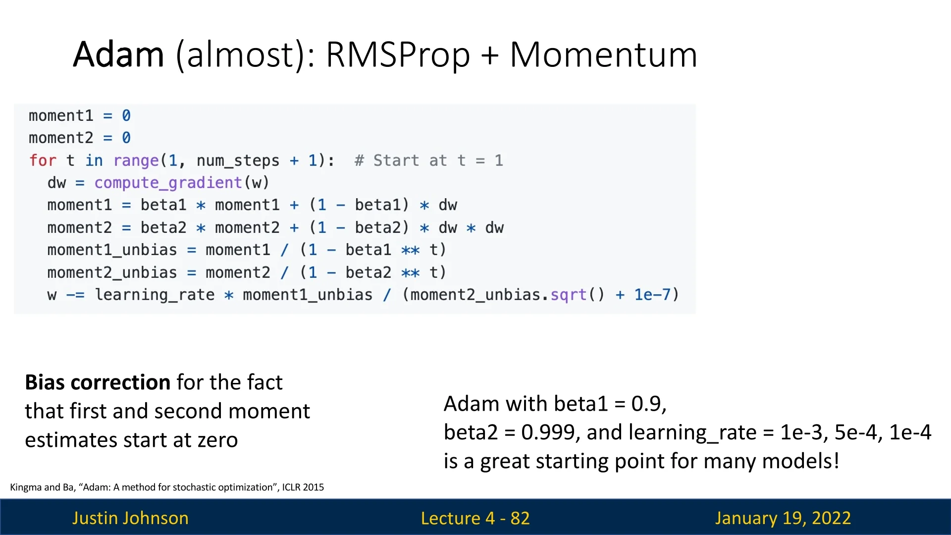
4.12.3 Bias Correction

Adam applies bias correction to address the issue of initialization bias for \( m_0 = 0 \) and \( v_0 = 0 \). Without correction, the estimates for \( m_t \) and \( v_t \) would be biased toward zero, especially in the early stages of training. This is a huge issue, as the steps in the beginning of the optimization process will thus be undesirably large, and can even lead to overshooting or instability. Hence, for optimal performance bias correction is undoubtedly needed. Bias correction is computed as follows: \[ \hat {m}_t = \frac {m_t}{1 - \beta _1^t}, \quad \hat {v}_t = \frac {v_t}{1 - \beta _2^t}. \] The corrected moments are used to compute the parameter updates: \[ w_{t+1} = w_t - \frac {\eta }{\sqrt {\hat {v}_t} + \epsilon } \hat {m}_t. \] Here:

• \( \eta \): Learning rate.
• \( \epsilon \): Smoothing term (default \( 10^{-8} \)) to avoid division by zero.

4.12.4 Why Adam Works Well in Practice

Adam’s robustness lies in its ability to adaptively scale updates for each parameter while incorporating momentum.

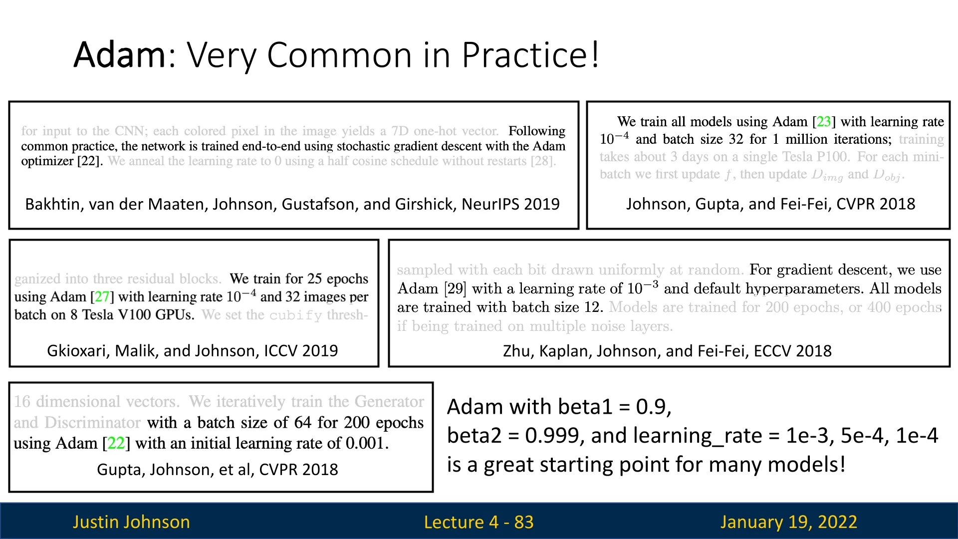
Figure 4.24 highlights the widespread adoption of Adam with default hyperparameters (\( \beta _1 = 0.9, \beta _2 = 0.999, \eta = 10^{-3} \mbox{ or } \eta = 10^{-4}\)) in numerous deep learning papers. These settings work well across a variety of tasks with minimal tuning.

4.12.5 Comparison with Other Optimizers

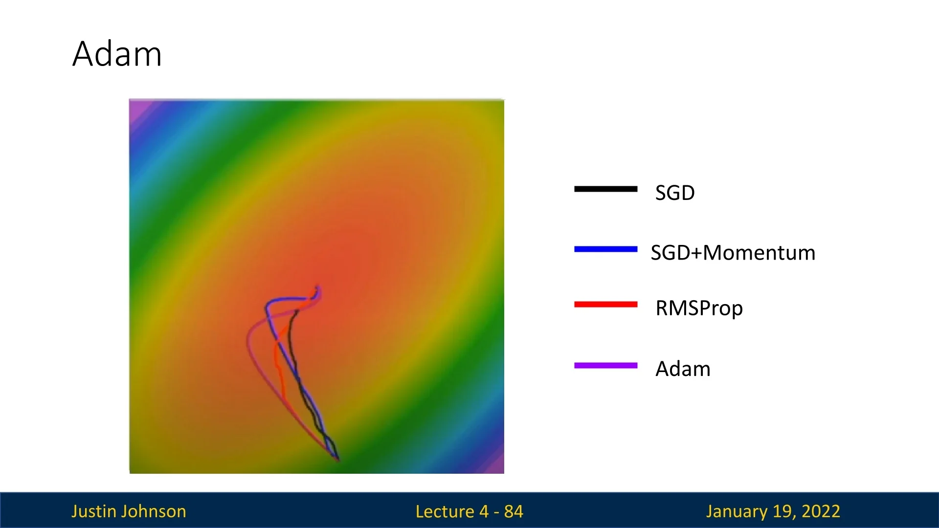
Figure 4.25 compares Adam with other optimizers like SGD, SGD+Momentum, and RMSProp. While all methods eventually converge, Adam typically converges faster, taking a more direct path to the minimum. It also handles noisy gradients better than momentum-based methods, resulting in fewer oscillations and faster recovery from overshooting. Regardless, it is crucial to remember that all the figures shown in this chapter are of 2 parameters only as we humans are limited to 3d. In very high dimensional landscapes, the behavior might greatly differ. As these are the common cases in deep learning, take this comparison with a grain of salt. It still is useful to gain some intuition regarding these optimization methods and their differences, but it’s important to not have too much fate in it.

4.12.6 Advantages of Adam

• Combines momentum and adaptive learning rates for robust optimization.
• Handles noisy gradients effectively, reducing oscillations.
• Requires minimal hyperparameter tuning, making it user-friendly for practitioners.
• Achieves faster and more stable convergence than earlier methods.

4.12.7 Limitations of Adam

Despite its strengths, Adam has some limitations:

• Overshooting: While less troublesome than in SGD+Momentum, Adam can still overshoot the minimum and take a while to recover.
• Memory Usage: Requires additional storage for \( m_t \) and \( v_t \), increasing memory overhead.

Looking Ahead While Adam is effective on its own, advanced variants like Nadam (Nesterov-accelerated Adam) and AdamW (Adam with weight decay) address specific issues, such as overshooting or generalization. However, for most applications, Adam remains a reliable and widely used optimizer in deep learning.

4.13 AdamW: Decoupling Weight Decay from L2 Regularization

4.13.1 Motivation for AdamW

While Adam is a widely used optimizer in deep learning, its integration with L2 regularization has been found problematic. Traditional Adam combines L2 regularization with weight updates during optimization. However, this approach can lead to unintended interactions:

• Magnitude Dependent Regularization: L2 regularization affects the moment estimates, leading to an implicit adjustment of the learning rate for parameters with larger magnitudes.
• Inconsistent Penalization: The coupling of weight decay and optimization can distort the intended regularization effect.

To address these issues, AdamW decouples weight decay from L2 regularization, treating weight decay as a distinct step in the optimization process. This separation ensures that weight decay consistently penalizes parameter magnitudes without interfering with moment estimates.

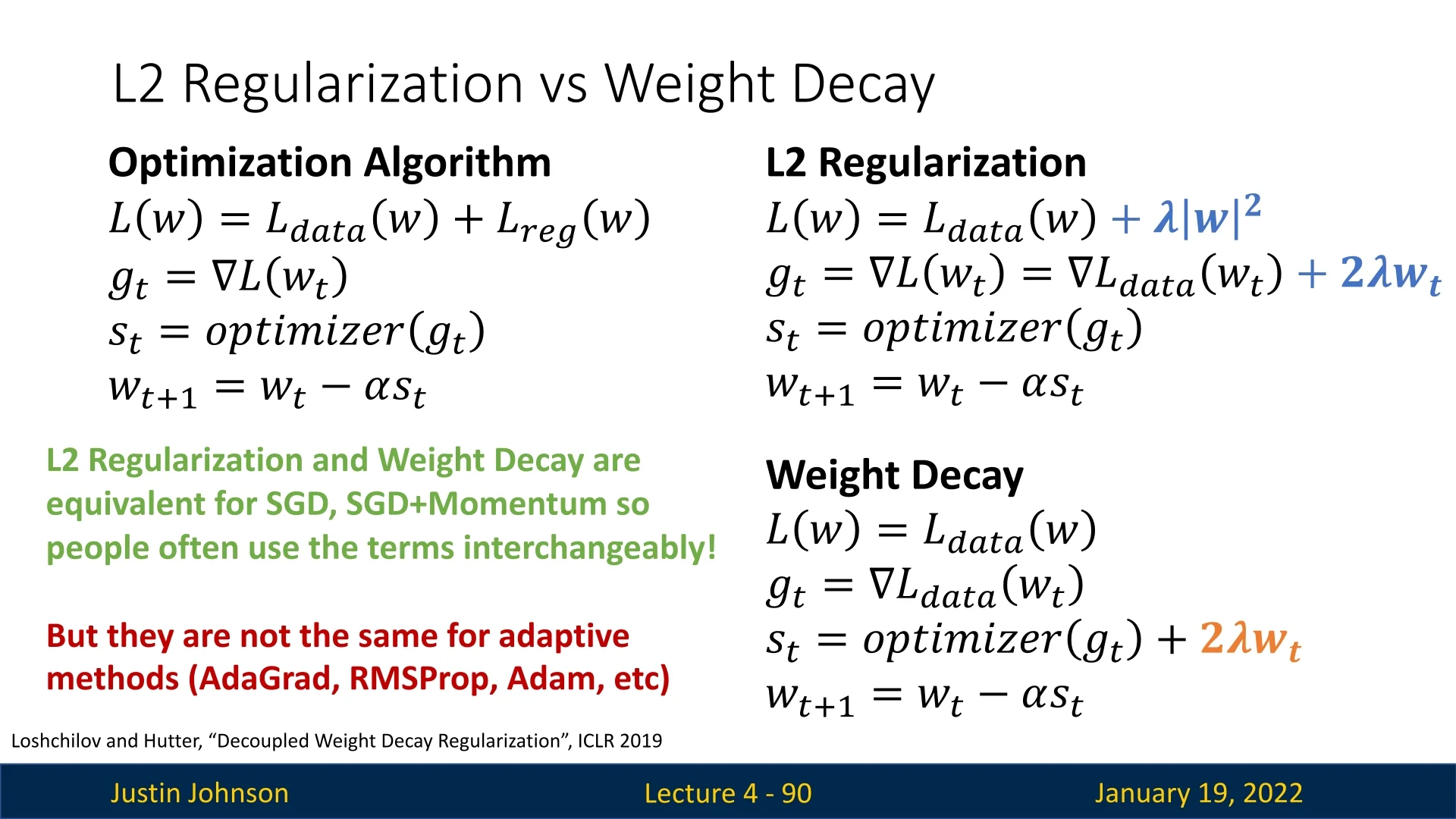
4.13.2 How AdamW Works

AdamW modifies the weight update rule by explicitly decoupling the weight decay term. The key steps are:

• Compute the gradient \( g_t \) of the loss with respect to the weights.
• Apply bias-corrected first and second moments, as in Adam: \[ \hat {m}_t = \frac {m_t}{1 - \beta _1^t}, \quad \hat {v}_t = \frac {v_t}{1 - \beta _2^t}. \]
• Update the weights using the Adam update rule, but subtract a scaled weight decay term: \[ w_{t+1} = w_t - \eta \left ( \frac {\hat {m}_t}{\sqrt {\hat {v}_t} + \epsilon } + \lambda w_t \right ), \] where \( \lambda \) is the weight decay coefficient.

This decoupling ensures that the weight decay term acts as a pure penalization of large weights, independent of the adaptive learning rate mechanism.

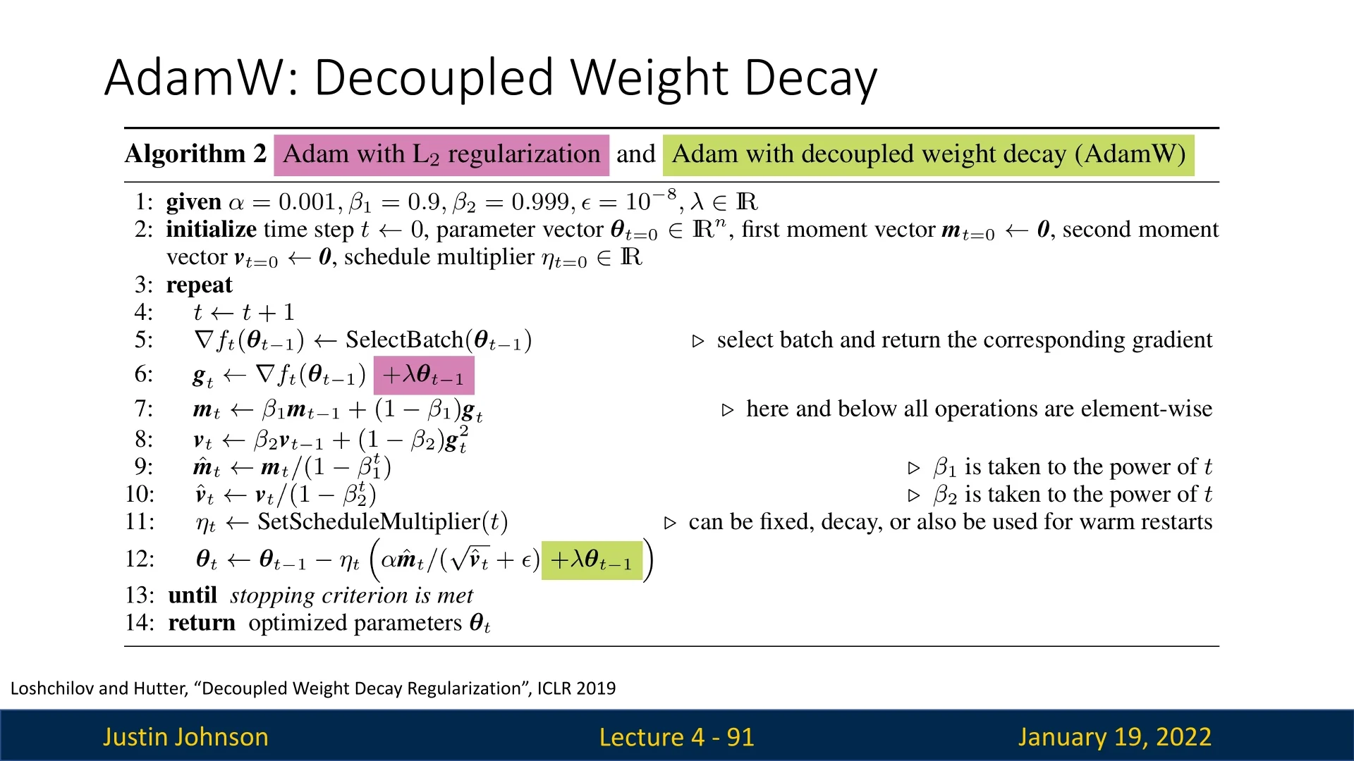
4.13.3 Note on Weight Decay in AdamW

In the pseudo-code, the violet term in line 6 represents L2 regularization as it is typically implemented in Adam (not AdamW) in many deep learning frameworks. This term adds the weight decay directly to the loss function, and its gradient is incorporated into the computation of the total gradients \( g \). However, this approach introduces unintended consequences:

• Entanglement with Moving Averages: When the regularization term is included in the loss, the moving averages \( m \) and \( v \) (used for the first and second moments of gradients) track not only the gradients of the loss function but also the contributions from the weight decay term.

• Normalization Effect: This interaction impacts the update step. Specifically, in Adam, line 12 of the pseudo-code includes \( \lambda \theta _{t-1} \) in the numerator, and this term gets normalized by \( \sqrt {\hat {v}_t} \) in the denominator. Consequently:

  • Weights with large or highly variable gradients (corresponding to a larger \( \hat {v}_t \)) experience less regularization.
  • Weights with small or slowly changing gradients are penalized more heavily, even though this may not align with the intended regularization behavior.

This phenomenon undermines the effectiveness of L2 regularization in Adam, deviating from the intended proportionality of weight decay to the weight magnitude. It explains why models trained with Adam sometimes generalize less effectively than those trained with SGD, which handles L2 regularization as intended.

4.13.4 The AdamW Improvement

To address this issue, the authors of AdamW propose a critical modification: decoupling the weight decay from the gradient computation. Specifically:

• The violet term in line 6 is removed from the gradient computation.
• The green term in line 12 applies weight decay as a direct adjustment to the parameter update after controlling for parameter-wise step sizes.

This decoupling ensures that:

1.

Weight decay acts only as a direct proportional penalty to the parameter values, independent of the gradient dynamics.

2.

The moving averages \( m \) and \( v \) track only the gradients of the loss function, preserving their intended role.

4.13.5 Advantages of AdamW

Experimental results demonstrate that AdamW:

• Improves training loss compared to standard Adam.
• Yields models that generalize significantly better, comparable to those trained with SGD+Momentum.
• Retains Adam’s adaptability and efficiency for large-scale optimization tasks.

By resolving the shortcomings of L2 regularization in Adam, AdamW has become the recommended default optimizer for many deep learning problems.

4.13.6 Why AdamW is the Default Optimizer

AdamW combines the adaptive learning rates of Adam with the benefits of properly implemented weight decay, making it a powerful default optimizer for many deep learning tasks:

• Works well out-of-the-box with minimal hyperparameter tuning.
• Handles large-scale, non-convex problems effectively.
• Avoids pitfalls of traditional L2 regularization in Adam, such as learning rate distortion.

4.13.7 Limitations of AdamW

Despite its advantages, AdamW is not without challenges:

• Requires careful tuning of the weight decay coefficient \( \lambda \) for optimal performance.
• Sensitive to learning rate schedules, particularly for complex architectures.

4.14 Second-Order Optimization

4.14.1 Overview of Second-Order Optimization

First-order optimization methods rely exclusively on gradient information—the first derivative of the loss function—to iteratively minimize the objective. Second-order optimization extends this idea by incorporating information from the Hessian matrix, which captures the second derivatives of the loss function and thus describes the curvature of the loss landscape.

What the Hessian Reveals The Hessian matrix \( H = \nabla ^2 L(W) \) expresses how the gradient changes as the parameters \( W \) vary, effectively describing the local geometry of the optimization landscape. Its eigenvalues \(\lambda _i\) and eigenvectors reveal curvature along each principal direction:

• Small \(\lambda _i \approx 0\): Flat or plateau regions where the loss changes slowly; large steps can safely be taken.
• Large positive \(\lambda _i\): Sharp curvature (“narrow bowl”) where the loss rises steeply; small steps are needed to remain stable.
• Negative \(\lambda _i\): Directions of negative curvature—saddle points where the surface curves upward in some directions and downward in others.

In this way, the eigenvalues of \(H\) serve as curvature coefficients, determining how sensitive the loss is to parameter changes along each axis.

4.14.2 Quadratic Approximation Using the Hessian

Second-order methods use curvature information by locally approximating the loss function with a quadratic model around the current point \( W_t \): \[ L(W) \approx L(W_t) + \nabla L(W_t)^\top (W - W_t) + \tfrac {1}{2}(W - W_t)^\top H(W_t) (W - W_t), \] where:

• \( \nabla L(W_t) \) is the gradient at the current parameters, representing the slope.
• \( H(W_t) \) is the Hessian, representing local curvature of the loss surface.

Minimizing this quadratic approximation leads to a curvature-aware update: \[ W_{t+1} = W_t - H(W_t)^{-1} \nabla L(W_t), \] or equivalently, \[ \Delta W = -H^{-1}\nabla L(W_t). \] This update rescales and rotates the gradient according to the curvature, automatically adapting both the direction and the magnitude of each step.

Geometric Intuition Each eigenvalue–eigenvector pair \((\lambda _i, v_i)\) of the Hessian defines an axis of local curvature:

• Flat directions (\(\lambda _i \approx 0\)): The loss changes slowly—large steps accelerate progress.
• Steep directions (\(\lambda _i \gg 0\)): The loss rises sharply—steps must be small to prevent oscillation or divergence.
• Saddle directions (\(\lambda _i < 0\)): The loss decreases along one dimension but increases along another—steps must be corrected to avoid instability.

Thus, second-order updates scale steps inversely with curvature: \[ \mbox{Step size in direction } v_i \propto \tfrac {1}{\lambda _i}. \] This geometric adaptivity makes second-order methods inherently more efficient and stable in complex, anisotropic landscapes.

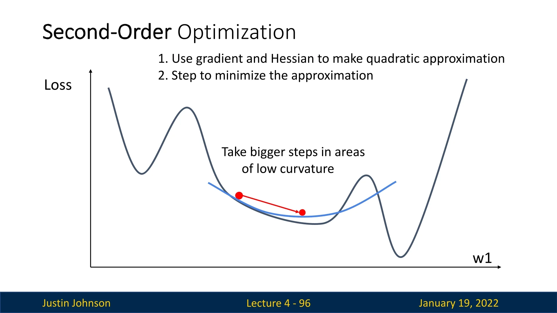
Why Second-Order Methods Converge Faster The power of second-order optimization lies in its awareness of the loss landscape’s geometry. First-order methods, like gradient descent, follow only the steepest direction, which can cause inefficient zigzagging in elongated valleys where curvature differs greatly across directions. In contrast, second-order methods precondition the gradient by \(H^{-1}\), normalizing curvature:

• In high-curvature regions (large \(\lambda _i\)): Updates are dampened to prevent overshooting.
• In flat regions (small \(\lambda _i\)): Updates are amplified for faster movement.

This curvature-based scaling effectively “spherizes” the loss landscape, enabling the optimizer to take near-direct routes to minima rather than oscillating between steep walls.

When the Hessian is well-conditioned—that is, its eigenvalues are moderate and roughly similar—Newton-type updates can achieve convergence in far fewer iterations than gradient descent. For purely quadratic functions, Newton’s method finds the minimum in a single step.

Intuitively, gradient descent is like feeling one’s way down a mountain using only the slope underfoot, while second-order methods also sense how the slope bends—taking large strides on flat terrain and shorter, precise ones in steep ravines—to reach the valley floor far more efficiently.

4.14.3 Practical Challenges of Second-Order Methods

Despite their theoretical appeal, second-order methods face severe computational limitations in modern deep learning:

• High Dimensionality: The Hessian contains \(O(N^2)\) elements for \(N\) parameters, making it impossible to store for networks with millions or billions of weights.
• Matrix Inversion Cost: Computing \(H^{-1}\) scales as \(O(N^3)\), which is prohibitive even for medium-scale models.
• Ill-Conditioning: When eigenvalues vary drastically in magnitude, inversion becomes numerically unstable and leads to poor updates.

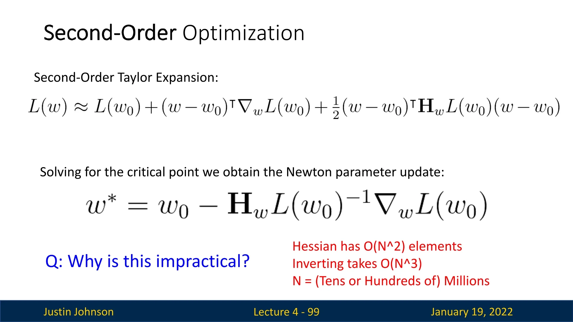
While full second-order methods are impractical for deep networks, their ideas inspire efficient approximations used in practice.

4.14.4 First-Order Methods Approximating Second-Order Behavior

Many modern optimizers mimic curvature-aware behavior using only first-order information:

• Adagrad: Adapts per-parameter learning rates based on the historical magnitude of gradients, approximating diagonal curvature.
• SGD with Momentum: Smooths gradients over time, implicitly incorporating curvature along dominant directions.
• Adam: Combines adaptive learning rates and momentum to emulate some second-order dynamics while remaining computationally lightweight.

In essence, these methods capture part of the benefit of second-order optimization—adaptive scaling and stability—without explicitly computing or inverting the Hessian, making them the default choice for training large-scale deep networks.

4.14.5 Improving Second-Order Optimization: BFGS and L-BFGS

Methods like Broyden–Fletcher–Goldfarb–Shanno (BFGS) and its limited-memory variant L-BFGS have been developed to address the challenge of expensive computations and high memory consumption. These methods approximate the Hessian matrix to reduce memory and computation costs, making second-order techniques more feasible in certain scenarios.

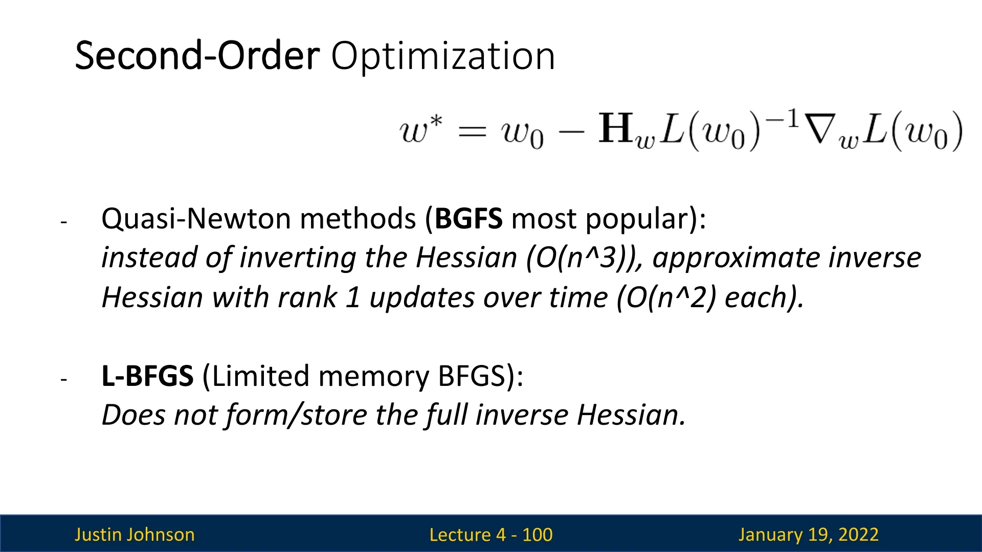
Although getting into the bits and bytes of BFGS and L-BFGS is outside the scope of the lecture and this summary, it’s still interesting to provide a high-level overview of the two algorithms and what they improve in second-order optimization methods.

BFGS: An Approximation of the Hessian Matrix

BFGS is an iterative optimization algorithm that avoids the explicit computation of the Hessian matrix. Instead:

• It uses gradient information to iteratively build an approximation of the inverse Hessian.
• Updates are performed using a rank-two update rule, ensuring that the approximation remains symmetric and positive definite.
• The update rule is efficient, allowing the algorithm to adaptively refine its estimates of the curvature.

While BFGS reduces the computational burden compared to exact second-order methods, it still requires \( O(N^2) \) storage for the approximate Hessian, making it unsuitable for high-dimensional problems.

L-BFGS: Reducing Memory Requirements

To address the memory limitations of BFGS, the Limited-Memory BFGS (L-BFGS) algorithm was introduced. Instead of storing the entire approximate Hessian, L-BFGS:

• Maintains only a few vectors from the most recent iterations, significantly reducing memory requirements.

• Requires \( O(kN) \) storage, where \( k \) is the number of vectors retained and is much smaller than \( N \) (typically \( k \approx 10 \)).
• Iteratively updates the approximation using gradient differences and weight updates from recent steps.

This makes L-BFGS particularly useful for optimization problems with moderate dimensionality, such as natural language processing or small-scale machine learning tasks.

Advantages and Limitations of BFGS and L-BFGS

Advantages:

• Adaptive Step Sizes: BFGS and L-BFGS use curvature information to adjust step sizes, improving convergence rates compared to first-order methods.
• Efficiency in Moderate Dimensions: L-BFGS reduces memory usage, enabling the use of second-order ideas in medium-scale problems.

Limitations:

• Still Computationally Expensive: Even L-BFGS requires \( O(kN) \) storage and computations, making it impractical for very high-dimensional problems such as deep learning.
• Not Robust for Non-Convex Problems: Second-order methods, including BFGS and L-BFGS, can still struggle with saddle points and highly non-convex landscapes commonly encountered in deep learning.

Applications of L-BFGS

L-BFGS remains a valuable tool for optimization problems where:

• The parameter space is not excessively high-dimensional.
• Precise curvature information is advantageous, such as in logistic regression or support vector machines.
• Fine-tuning is required near convergence to achieve high precision.

4.14.6 Summary of Second-Order Optimization Approaches

Second-order optimization methods, such as BFGS and L-BFGS, provide valuable insights into the curvature of the loss landscape, enabling adaptive step sizes and improved convergence rates. However, their computational and memory requirements make them impractical for large-scale machine learning problems. For such tasks, first-order methods like Adam remain the standard due to their scalability and effectiveness.