Lecture 15: Image Segmentation
15.1 From Object Detection to Segmentation
In the previous chapter, we explored object detection, where the goal was to localize and classify objects within an image using bounding boxes. Object detection models such as Faster R-CNN [539] and YOLO [534] predict discrete object regions but do not assign labels to every pixel. However, many real-world applications require a finer-grained understanding beyond bounding boxes. This leads us to the problem of image segmentation, where the task is to assign a category label to every pixel in the image.
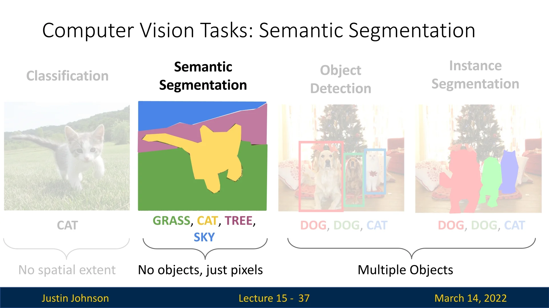
As shown in Figure 15.1, segmentation can be divided into two primary tasks:
- Semantic segmentation: Assigns a category label to each pixel but does not differentiate between instances of the same class.
- Instance segmentation: Extends semantic segmentation by distinguishing individual object instances.
We begin by studying semantic segmentation because it serves as the foundation for understanding pixel-wise classification. Unlike instance segmentation, which requires distinguishing between different objects of the same category, semantic segmentation focuses solely on identifying the type of object at each pixel. By first mastering the fundamental principles of pixel-wise classification, we can later build upon them to incorporate instance-level distinctions.
Enrichment 15.2: Why is Object Detection Not Enough?
Consider an autonomous vehicle navigating through a crowded urban environment. Object detection is a crucial first step: it draws bounding boxes around pedestrians, vehicles, and traffic signs, and already provides coarse spatial awareness (for example, that a pedestrian is somewhere near the curb rather than in the middle of the road). However, this level of understanding is still not sufficient for safe, fine-grained decision-making:
- Bounding boxes are coarse approximations. A bounding box is a rectangle that roughly encloses an object, not its true shape. In many cases this is enough to know that a pedestrian is “near the road”, but in safety-critical edge cases—such as a foot just crossing the curb versus standing safely on the sidewalk—the box does not reveal the precise contact boundary between pedestrian and road.
- Occlusions and overlaps create ambiguity. When objects overlap (e.g., a cyclist partially hidden behind a parked car), their bounding boxes may intersect or fragment. From boxes alone, it is hard to infer which pixels belong to which object, who is in front or behind, and exactly where the free space lies between them.
- No labels for “stuff” and free space. Object detection focuses on discrete, countable “things” (cars, pedestrians, traffic lights), but leaves the background unlabeled. It does not differentiate drivable road surface from sidewalks, bike lanes, grass, or curbs at the pixel level, even though this information is crucial for path planning and rule-following (e.g., staying within the lane markings).
Semantic segmentation addresses these limitations by assigning a class label to every pixel in the image. Instead of just knowing that “there is a pedestrian in this box,” the model produces a dense map indicating exactly which pixels are road, sidewalk, pedestrian, car, or building. This pixel-wise understanding provides the geometric and contextual detail needed for precise obstacle avoidance, free-space estimation, and safe navigation in complex scenes.
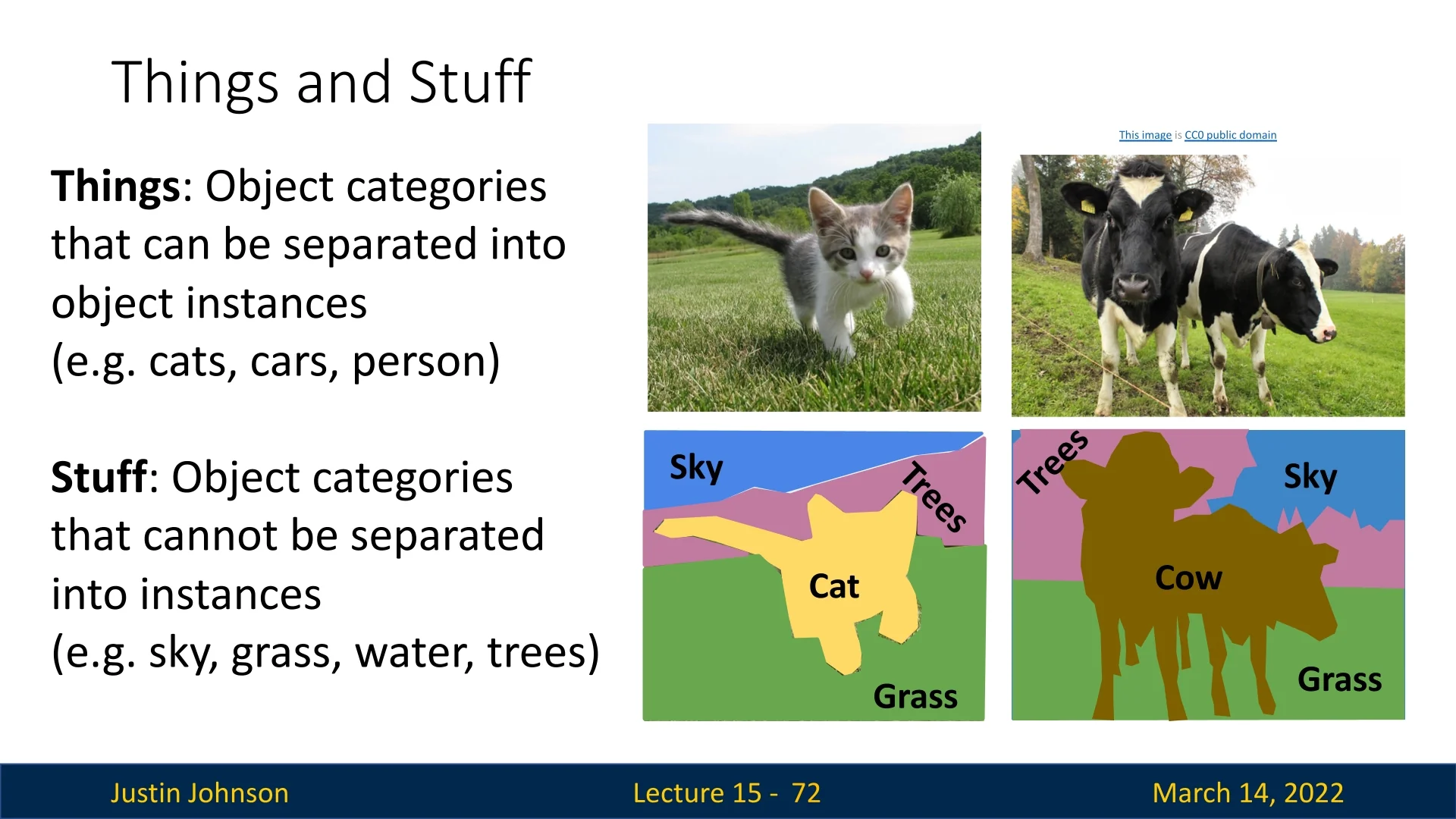
In Figure 15.2, we see a breakdown of image elements into things (object categories that can be separated into instances, such as cars, pedestrians, trees) and stuff (regions that lack clear boundaries, such as sky, road, grass). This pixel-level distinction enables applications such as lane detection, drivable area estimation, and pedestrian tracking, all of which contribute to safer and more efficient navigation.
The next sections will cover the fundamental methods used in segmentation, beginning with semantic segmentation, before proceeding to instance segmentation.
15.3 Advancements in Semantic Segmentation
In this section, we explore the evolution of semantic segmentation techniques, focusing on solutions that are convolutional neural networks (CNNs) based, reaching to more contemporary architectures. While CNNs have been foundational in image processing tasks, recent advancements indicate that transformer-based models have achieved superior accuracy in segmentation tasks, including semantic segmentation. These will only be discussed in future parts of this document.
15.2.1 Early Approaches: Sliding Window Method
A straightforward yet inefficient approach to semantic segmentation involves the sliding window technique. In this method, for each pixel in the image, a patch centered around the pixel is extracted and classified using a CNN to predict the category label of the center pixel.
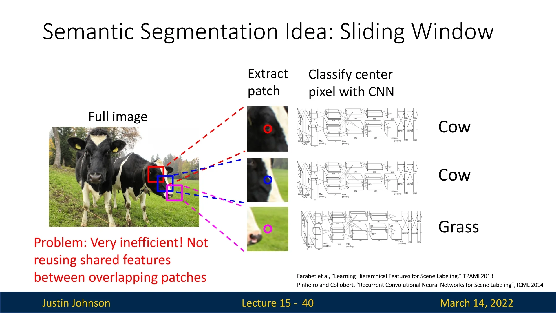
As depicted in Figure 15.3, this approach is computationally expensive because it fails to reuse shared features between overlapping patches, leading to redundant calculations.
15.2.2 Fully Convolutional Networks (FCNs)
To address the inefficiencies of the sliding window method, Fully Convolutional Networks (FCNs) were introduced to the task [402]. FCNs utilize a fully convolutional backbone to extract features from the entire image, maintaining the spatial dimensions throughout the layers by employing same padding and 1x1 convolutions. The network outputs a feature map with dimensions corresponding to the input image, where each channel represents a class. The final classification for each pixel is obtained by applying a softmax function followed by an argmax operation across the channels.
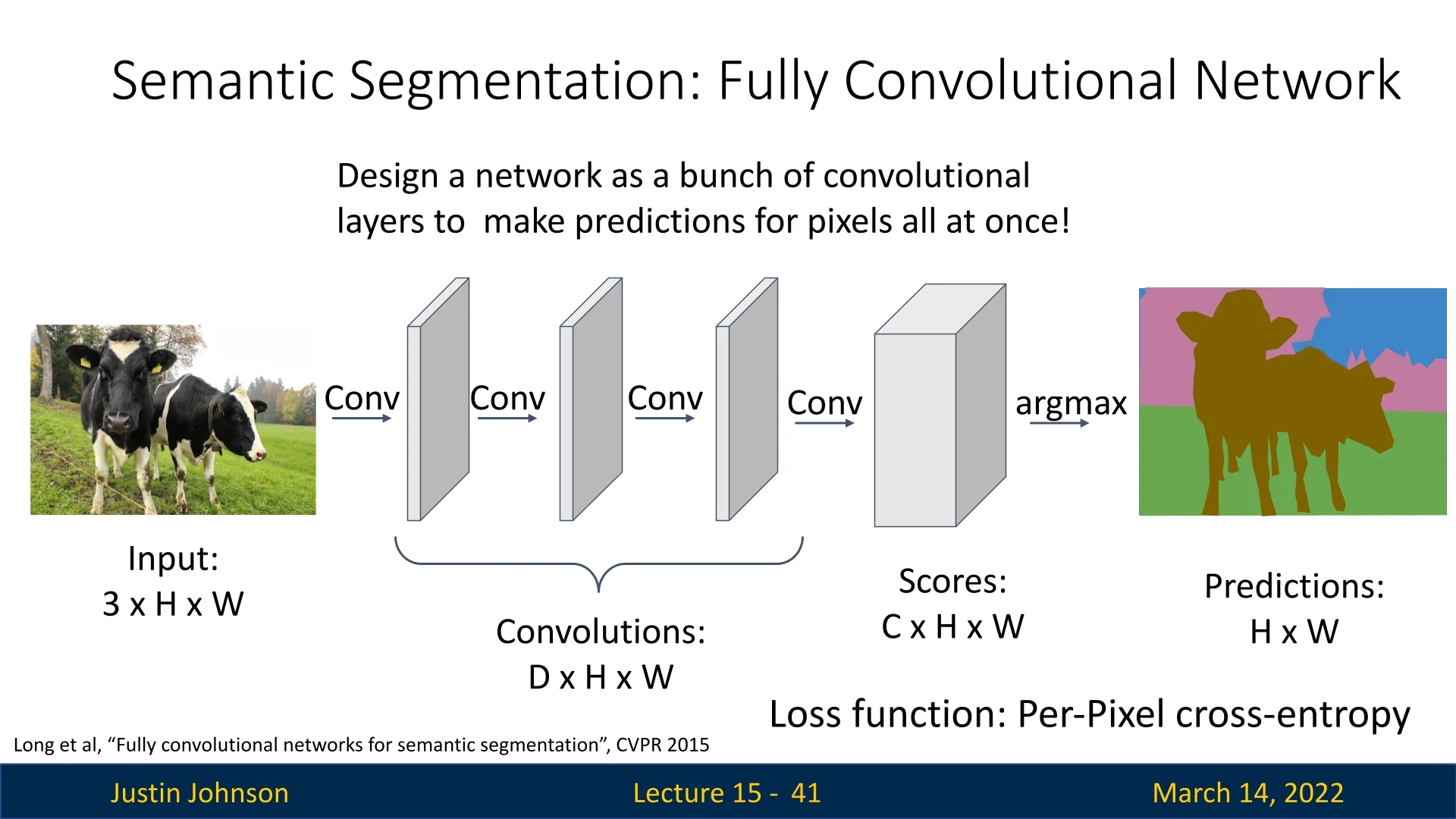
Training is conducted using a per-pixel cross-entropy loss, comparing the predicted class probabilities to the ground truth labels for each pixel.
15.2.3 Challenges in FCNs for Semantic Segmentation
Despite their advancements, FCNs encounter specific challenges:
- Limited Receptive Field: The effective receptive field size grows linearly with the number of convolutional layers. For instance, with \(L\) layers of 3x3 convolutions, the receptive field is \(1 + 2L\), which may be insufficient for capturing global context.
- Computational Cost: Performing convolutions on high-resolution images is computationally intensive. Architectures like ResNet address this by aggressively downsampling the input, but this can lead to a loss of spatial detail.
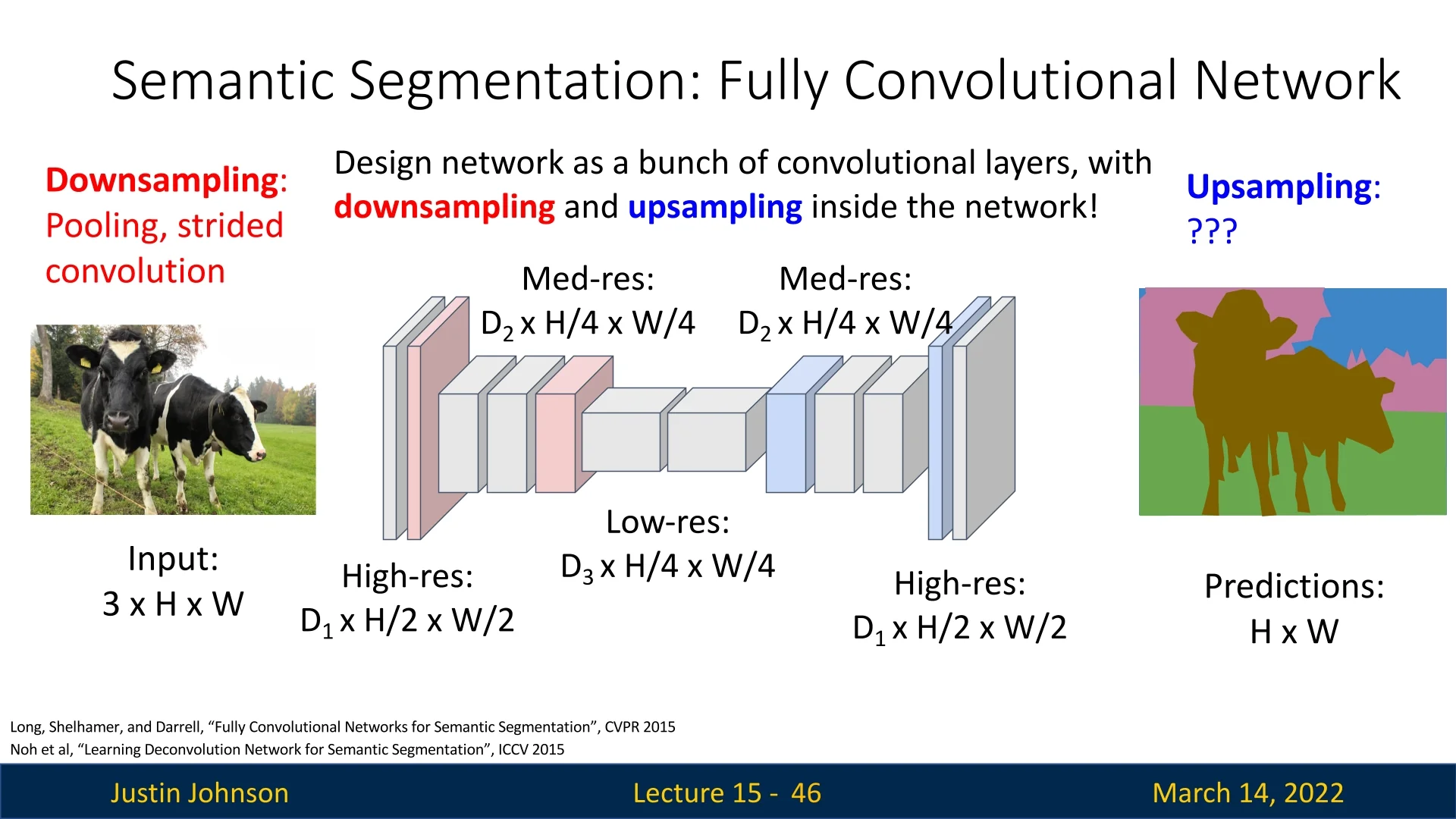
15.2.4 Encoder-Decoder Architectures
To overcome these challenges, encoder-decoder architectures have been proposed, such as the model by Noh et al. [468]. These networks consist of two main components:
- Encoder: A series of convolutional and pooling layers that progressively downsample the input image, capturing high-level semantic features while expanding the receptive field.
- Decoder: A sequence of upsampling operations, including unpooling and deconvolutions, that restore the spatial dimensions to match the original input size, enabling precise localization for segmentation.
The encoder captures rich, abstract feature representations by reducing spatial resolution while increasing feature depth, whereas the decoder reconstructs fine-grained spatial details necessary for accurate per-pixel predictions.
While this encoder-decoder design is applied here for semantic segmentation, it is a widely used architectural pattern in deep learning and extends to many other tasks. For example:
- Machine Translation: Transformer-based sequence-to-sequence models such as T5 [517] and BART [334] employ an encoder to process input text and a decoder to generate translated output.
- Medical Image Analysis: U-Net [549] applies an encoder-decoder structure for biomedical image segmentation, achieving precise boundary delineation in tasks like tumor segmentation.
- Anomaly Detection: Autoencoders use an encoder to learn compressed feature representations and a decoder to reconstruct inputs, enabling anomaly detection by identifying discrepancies between the input and reconstruction.
- Super-Resolution and Image Generation: Models like SRGAN [327] employ an encoder to extract image features and a decoder to generate high-resolution outputs.
As we continue, we will encounter various adaptations of this fundamental encoder-decoder structure, each tailored to the specific requirements of different tasks.
15.4 Upsampling and Unpooling
To enhance spatial resolution in feature maps, we employ upsampling techniques. Until now in this course, we have not introduced any method for systematically enlarging the spatial dimensions of tensors in a meaningful way. While we previously used bilinear interpolation to project proposals onto feature maps after downsampling ([ref]), we have yet to explore how such techniques can be adapted for general upsampling—something we will examine in later sections.
Although we can increase tensor size using zero-padding along the borders, this does not introduce any new spatial information or recover lost details, making it ineffective for true upsampling. Instead, we require dedicated upsampling methods that intelligently restore missing details while preserving spatial coherence. Throughout this section, we will explore various approaches that allow us to increase resolution effectively, ensuring that the upsampled feature maps retain meaningful information.
Do Interpolated Pixels Need to be “Valid” Image Values?
All of the upsampling and unpooling methods we have discussed (nearest neighbor, bilinear, bicubic, transposed convolution, etc.) operate in continuous space: they produce real-valued outputs by combining neighboring pixels or features with real-valued weights. This naturally raises two related questions:
- 1.
- What happens if the resulting pixel/feature values are non-integer or fall outside the usual image range?
- 2.
- When (if ever) do we need to enforce that the upsampled result is a valid image (e.g., integer RGB values in \([0, 255]\))?
Inside a neural network: real-valued feature maps are perfectly fine Within a convolutional network, tensors represent features, not necessarily display-ready images. In this setting:
- Feature maps are typically stored as 32-bit floating-point values, and can take on any real value (positive or negative, large or small).
- Upsampling operations (nearest neighbor, bilinear, bicubic, transposed convolution) simply produce new floating-point values. There is no requirement that these be integers or lie within a specific range; subsequent layers and nonlinearities will transform them further.
- Any normalization or scaling applied to the input (e.g., mapping RGB values from \([0,255]\) to \([0,1]\) or standardizing to zero mean and unit variance) is usually inverted only at the very end, if we want to visualize or save an image.
From this perspective, “non-integer” or slightly out-of-range values are not a problem at all during intermediate processing: the network is trained end-to-end to work with these continuous-valued feature maps.
At the output: producing a valid image for visualization or storage
The situation changes when the goal is to produce a valid image as the final output (e.g., in super-resolution, image-to-image translation, or generative models). In that case, we typically want:
- Pixel values in a fixed range (for example \([0,1]\) or \([0,255]\)).
- Integer-valued pixels if we are saving to standard formats (e.g., 8-bit uint8 RGB).
Common strategies in this case are:
- Constrain the range with an activation: Use a final activation such as \(\sigma (\cdot )\) (sigmoid) to map outputs to \([0,1]\), or \(\tanh (\cdot )\) to map to \([-1,1]\). During training, the loss is computed against normalized target images in the same range.
-
Post-processing after the network: Allow the network to output unconstrained real values, then:
- 1.
- De-normalize (invert any input normalization, e.g. multiply by standard deviation and add mean).
- 2.
- Clamp values to the valid range, e.g. \(\mbox{pixel} \leftarrow \min (\max (\mbox{pixel}, 0), 1)\) or \([0,255]\).
- 3.
- Quantize to integers if needed, e.g. \(\mbox{pixel}_{\mbox{uint8}} = \mbox{round}(255 \cdot \mbox{pixel}_{[0,1]})\).
- Handling overshoot in higher-order interpolation: Methods like bicubic interpolation can produce values slightly outside the original range (due to oscillatory cubic kernels). In classical image processing and in deep learning code, the standard remedy is simple clamping before display or saving.
In other words, when we care about producing a valid, displayable image, validity is enforced at the very end by range restriction and (optionally) quantization—not by changing the upsampling method itself.
Summary: feature maps vs. final images To summarize:
- For internal feature maps, non-integer and even slightly out-of-range values are entirely acceptable; the network treats them as continuous signals and learns to use them.
- For final image outputs, we typically normalize during training and then de-normalize, clamp to a valid range, and quantize at inference time to obtain a proper image representation (e.g., 8-bit RGB).
Thus, all of the upsampling and unpooling methods discussed in this chapter can be used without modification inside a network; concerns about “valid pixels” are addressed at the output layer or in a simple post-processing step when we need a real image rather than a learned feature map.
A crucial variant of upsampling is unpooling, which aims to reverse the effects of pooling operations. While pooling reduces resolution by discarding spatial details, unpooling attempts to restore them, facilitating fine-grained reconstruction of object boundaries. However, unpooling alone is often insufficient for producing smooth and accurate feature maps, as it merely places values in predefined locations without estimating missing information. This can result in reconstruction gaps, blocky artifacts, or unrealistic textures. As we will see, more advanced upsampling techniques address these shortcomings by incorporating interpolation and learnable transformations.
In the decoder architecture proposed by Noh et al., unpooling plays a fundamental role in progressively recovering lost spatial information. It bridges the gap between the high-level semantic representations learned by the encoder and the dense, pixel-wise predictions required for precise classification.
In the following sections, we explore various upsampling strategies, beginning with fundamental unpooling techniques and gradually progressing toward more advanced methods.
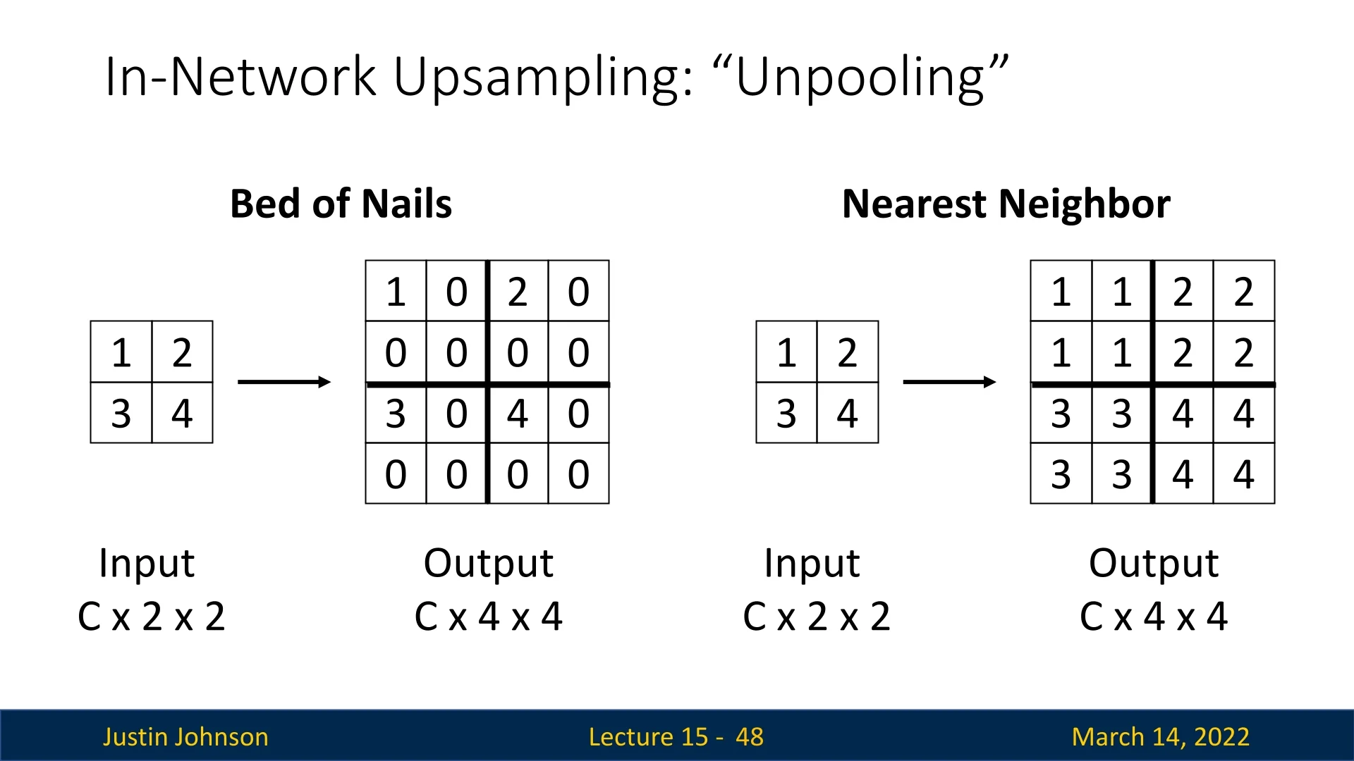
15.3.1 Bed of Nails Unpooling
One of the simplest forms of unpooling is known as Bed of Nails unpooling. To illustrate the concept, consider the following example: We’re given an input tensor of size \(C \times 2 \times 2\), and our objective is to produce an output tensor of size \(C \times 4 \times 4\).
The method follows these steps:
- An output tensor of the desired size is initialized with all zeros.
- The output tensor is partitioned into non-overlapping regions, each corresponding to a single value from the input tensor. The size of these regions is determined by the upsampling factor \(s\), which is the ratio between the spatial dimensions of the output and the input. For example, if the input is \(H \times W\) and the output is \(sH \times sW\), then each region in the output has size \(s \times s\).
- Each value from the input tensor is placed in the upper-left corner of its corresponding region in the output.
- All remaining positions are left as zeros.
The term ”Bed of Nails” originates from the characteristic sparse structure of this unpooling method, where non-zero values are positioned in a regular grid pattern, resembling nails protruding from a flat surface.
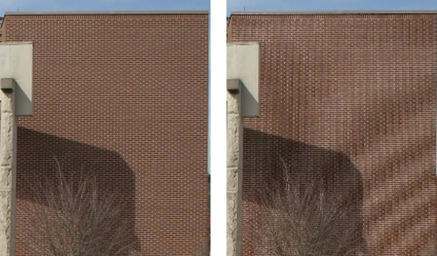
Limitations of Bed of Nails Unpooling While conceptually simple, Bed of Nails unpooling suffers from a critical flaw: it introduces severe aliasing, which significantly degrades the quality of the reconstructed feature maps. By sparsely placing input values into an enlarged output tensor and filling the remaining positions with zeros, this method results in a highly discontinuous representation with abrupt intensity changes. These gaps introduce artificial high-frequency components, making it difficult to recover fine spatial details and leading to distorted reconstructions.
The primary drawbacks of Bed of Nails unpooling are:
- Sparse Representation: The method leaves large gaps of zeros between meaningful values, creating an unnatural, high-frequency pattern that distorts spatial information.
- Abrupt Intensity Shifts: The sharp transitions between non-zero values and surrounding zeros introduce edge artifacts, leading to aliasing effects such as jagged edges and moiré patterns.
- Loss of Fine Detail: The lack of interpolation prevents smooth reconstructions, making it difficult to recover object boundaries and subtle spatial features.
Because of these limitations, Bed of Nails unpooling is rarely used in practice. Its inability to provide a smooth, information-preserving reconstruction makes it unsuitable for tasks requiring high-quality feature map upsampling.
15.3.2 Nearest-Neighbor Unpooling
A more practical alternative to Bed of Nails unpooling is Nearest-Neighbor unpooling. Instead of placing a single value in the upper-left corner and filling the rest with zeros, this method copies the value across the entire corresponding region, ensuring a more continuous feature map.
The key advantages of Nearest-Neighbor unpooling include:
- Smoother Transitions: By replicating values across the upsampled regions, Nearest-Neighbor unpooling maintains spatial continuity. In contrast, Bed of Nails unpooling introduces sharp jumps between non-zero values and large zero-filled areas, which disrupts smooth feature propagation.
- Reduced Aliasing: The discontinuities introduced by zero-padding in Bed of Nails unpooling create artificial high-frequency patterns, leading to jagged edges and moiré artifacts. Nearest-Neighbor unpooling minimizes these distortions by ensuring a more uniform intensity distribution.
- Better Feature Preservation: Copying values instead of inserting zeros retains more useful information about the original feature map. Since features remain continuous rather than fragmented by empty gaps, spatial relationships between objects are better preserved.
These properties make Nearest-Neighbor unpooling a more effective choice than Bed of Nails, particularly for reducing aliasing effects. By ensuring smoother transitions and preventing artificial high-frequency noise, it produces cleaner and more reliable feature maps, making it more suitable for deep learning applications.
However, Nearest-Neighbor unpooling still has limitations. Since it simply copies values, it can produce blocky (unsmooth) artifacts and lacks the ability to generate new information between upsampled pixels. This makes it unsuitable for capturing fine details, especially when dealing with natural images or complex textures.
To achieve better reconstructions, more advanced upsampling methods are used. These include:
- Bilinear Interpolation: A smoother alternative that interpolates pixel values using a weighted average of neighboring points. We’ve already covered it extensively.
- Bicubic Interpolation: Extends bilinear interpolation by considering more neighbors and applying cubic functions for higher-quality results.
- Max Unpooling: A structured approach that retains important features by reversing pooling operations using stored indices.
- Transposed Convolution: A learnable upsampling technique that enables neural networks to reconstruct detailed feature maps through trainable filters.
In the following parts, we will explore each of these methods, highlighting their advantages and trade-offs in deep learning applications.
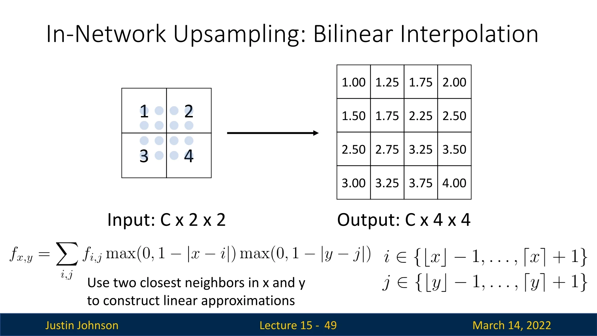
15.3.3 Bilinear Interpolation for Upsampling
While nearest-neighbor unpooling provides a simple way to upsample feature maps, it often introduces blocky artifacts due to the direct replication of values. A more refined approach is bilinear interpolation, which estimates each output pixel as a weighted sum of its surrounding neighbors, resulting in a smoother reconstruction.
Consider an input feature map of shape \(C \times H \times W\) and an output of shape \(C \times H' \times W'\), where the spatial dimensions are enlarged (\(H' > H\), \(W' > W\)). Unlike unpooling, which places values at predefined locations without interpolation, bilinear interpolation calculates each pixel’s intensity by considering its four nearest neighbors in the original input feature map.
Bilinear Interpolation: Generalized Case
Given an input feature map \(\mathbf {I}\) of size \(C \times H \times W\), we
define an upsampled feature map \(\mathbf {I'}\) of size \(C \times H' \times W'\).
To compute the value of a pixel at a location \((x', y')\) in the upsampled output, we follow these steps:
- Mapping to the Input Grid: The coordinate \((x', y')\) in the output feature map is mapped back to the corresponding position \((x, y)\) in the input space using the scaling factors: \[ x = \frac {x' (W - 1)}{W' - 1}, \quad y = \frac {y' (H - 1)}{H' - 1} \] where \(W'\) and \(H'\) are the new width and height, and \(W, H\) are the original dimensions.
- Identifying Neighboring Pixels: The four closest integer grid points that enclose \((x, y)\) are determined as: \[ a = (x_0, y_0), \quad b = (x_0, y_1), \quad c = (x_1, y_0), \quad d = (x_1, y_1) \] where: \[ x_0 = \lfloor x \rfloor , \quad x_1 = \lceil x \rceil , \quad y_0 = \lfloor y \rfloor , \quad y_1 = \lfloor y \rfloor . \] These four points form a bounding box around \((x, y)\).
- Computing the Interpolation Weights: Each neighboring pixel contributes to the final interpolated value based on its distance to \((x, y)\). The interpolation weights are computed as: \[ w_a = (x_1 - x) (y_1 - y), \quad w_b = (x_1 - x) (y - y_0) \] \[ w_c = (x - x_0) (y_1 - y), \quad w_d = (x - x_0) (y - y_0). \]
-
Normalization: To ensure that the weights sum to one, we apply a normalization factor: \[ \mbox{norm_const} = \frac {1}{(x_1 - x_0)(y_1 - y_0)}. \]
- Computing the Interpolated Value: The final interpolated intensity at \((x', y')\) is then computed as: \[ I'(x', y') = w_a I_a + w_b I_b + w_c I_c + w_d I_d. \]
Advantages and Limitations of Bilinear Interpolation
Bilinear interpolation offers clear improvements over nearest-neighbor unpooling when upsampling feature maps or images. Instead of simply copying the nearest value, each output pixel is computed as a weighted average of its four closest input pixels, with weights determined by geometric distance. This produces smoother transitions, reduces blocky artifacts, and better preserves local spatial relationships than nearest-neighbor methods.
However, bilinear interpolation also has important limitations. Because it relies on only four neighbors and uses simple linear weighting, it tends to blur high-frequency details: fine textures, sharp edges, and small-scale patterns can become softened. In effect, bilinear interpolation trades off blockiness for smoothness, but at the cost of some sharpness and detail.
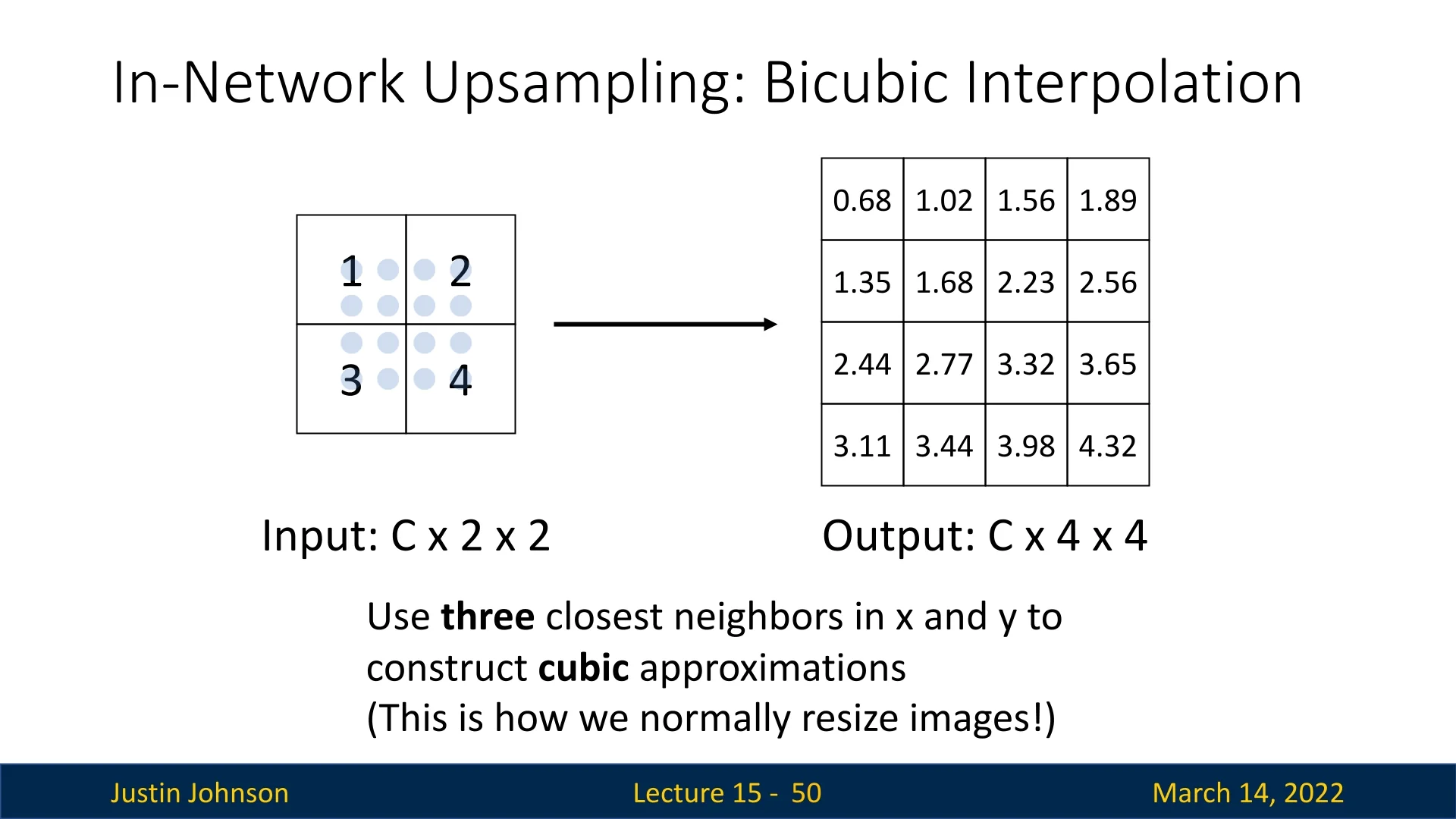
15.3.4 Bicubic Interpolation for Upsampling
Bicubic interpolation is a more advanced alternative to nearest-neighbor or bilinear upsampling. Instead of using just four neighbors, bicubic interpolation considers a \(4 \times 4\) neighborhood (16 pixels) around each output position and applies a cubic weighting function along each axis. This broader context and smoother weighting scheme allow the method to better respect local structure and produce sharper, more detailed upsampled results.
Why Bicubic Interpolation?
The wider support of bicubic interpolation directly addresses the limitations of bilinear interpolation. By aggregating information from sixteen neighboring pixels and using cubic (rather than linear) weights, bicubic interpolation can better preserve edges, reduce blurring, and maintain fine textures. For this reason, it is commonly used as a high-quality default for image resizing and is often preferred in deep learning pipelines when visually faithful, detail-preserving upsampling is important.
Mathematical Reasoning
Bicubic interpolation extends bilinear interpolation by introducing a cubic weighting function that smoothly distributes the contribution of each neighboring pixel. While bilinear interpolation assigns weights based purely on distance (linearly decreasing to zero), the cubic approach tailors these weights using a function that decays gradually, allowing pixels farther from the target position to still have a small but meaningful influence.
The commonly used weighting function is piecewise-defined:
\[ W(t) = \begin {cases} (a + 2)|t|^3 - (a + 3)|t|^2 + 1, & 0 \leq |t| < 1, \\ a|t|^3 - 5a|t|^2 + 8a|t| - 4a, & 1 \leq |t| < 2, \\ 0, & |t| \geq 2, \end {cases} \]
where \(a\) typically takes values around \(-0.5\) to balance smoothness and sharpness. The function ensures nearby pixels carry the most weight, while more distant neighbors still contribute smoothly rather than being abruptly excluded.
A concise visual and conceptual explanation can be found in this Computerphile video.
Bicubic Interpolation: Generalized Case
Assume we have an input feature map \(\mathbf {I}\) of size \(C \times H \times W\), and we wish to produce an upsampled map \(\mathbf {I'}\) of size \(C \times H' \times W'\). The bicubic interpolation proceeds as follows:
- 1.
- Coordinate Mapping: Map the output pixel location \((x',y')\) back to the corresponding floating-point coordinate \((x,y)\) in the input grid: \[ x = \frac {x'(W - 1)}{W' - 1}, \quad y = \frac {y'(H - 1)}{H' - 1}. \]
- 2.
- Neighbor Identification: Determine the \(\pm 1\) and \(\pm 2\) offsets around \(\lfloor x \rfloor \) and \(\lfloor y \rfloor \). This yields a \(4 \times 4\) set of pixels \(\{I_{i,j}\}\) centered near \((x,y)\).
- 3.
- Applying the Cubic Weights: Use the cubic function \(W(t)\) in both the \(x\) and \(y\) directions: \[ I'(x', y') = \sum _{i=-1}^{2}\sum _{j=-1}^{2} W(x - x_i)\,W(y - y_j)\,I_{i,j}. \]
Advantages and Limitations
Sharper Details and Continuity. By sampling a larger neighborhood with a smoothly decaying weight function, bicubic interpolation preserves finer structures, reduces artifacts, and transitions more smoothly across pixel boundaries than bilinear interpolation.
Better Texture Preservation. Rather than over-smoothing, bicubic interpolation better maintains texture information by assigning fractional influences to pixels farther than one unit away.
Non-Learnable. Despite these benefits, bicubic interpolation remains a fixed formula that cannot adapt to complex or domain-specific feature distributions in deep learning.
In contrast, max unpooling or learnable upsampling layers (we’ll learn about those in the following parts) can dynamically capture where and how to upscale feature maps.
Hence, while bicubic interpolation offers a clear advantage over simpler methods for image resizing tasks, its fixed nature can be sub-optimal in end-to-end neural networks that require trainable, context-dependent upsampling.
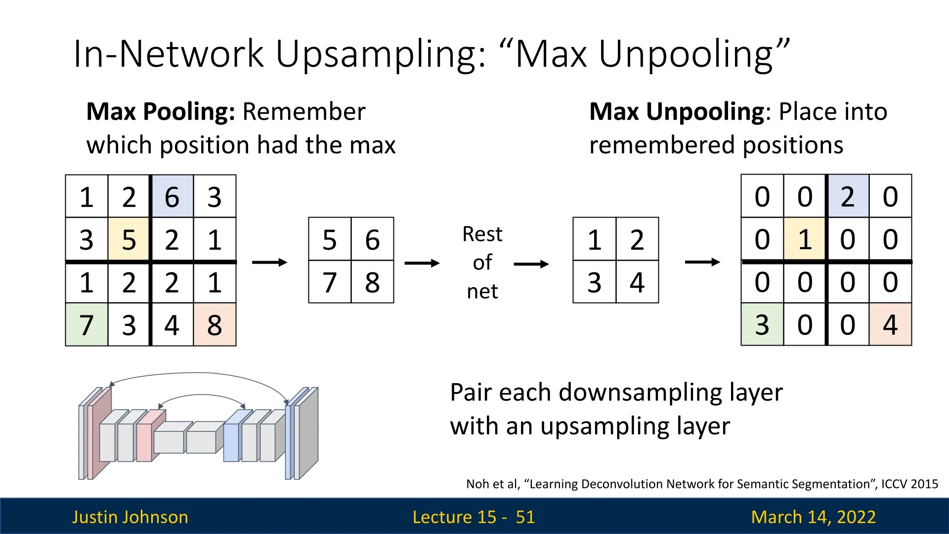
15.3.5 Max Unpooling
Max unpooling is an upsampling operation designed to “invert” max pooling as faithfully as possible. Instead of estimating new values via interpolation (as in bilinear or bicubic upsampling), max unpooling is a routing mechanism: it uses the indices of the maxima recorded during max pooling to place activations back into their original spatial locations, producing a sparse but geometrically aligned feature map.
Intuitively, max unpooling acts like a memory of where the network believed the most important responses were before downsampling. During encoding, max pooling keeps only the largest activation in each window and remembers where it came from. During decoding, max unpooling re-expands the feature maps and reinstates those activations exactly at the stored positions, filling all other locations with zeros. This preserves the encoder’s notion of “where things are” while deferring dense reconstruction to subsequent convolutions.
Max Unpooling in the DeconvNet of Noh et al. (ICCV 2015)
In the DeconvNet architecture proposed by Noh et al. [468], max unpooling layers are placed symmetrically to the max pooling layers of the encoder. Each pooling layer performs:
- Max pooling with switches: For each pooling window (e.g., \(2 \times 2\) with stride 2), the encoder selects the maximum activation and stores its index (row and column position) inside the window.
The corresponding max unpooling layer in the decoder then executes three conceptually simple steps:
- 1.
- Re-expand the spatial grid: The decoder allocates an upsampled feature map with the same spatial resolution as the pre-pooled feature map.
- 2.
- Place activations using indices: Each pooled activation is written back into the upsampled grid at the exact location indicated by its recorded index; all other positions in that pooling window are set to zero.
- 3.
- Refine sparsity via convolutions: This sparse, index-aligned map is passed through convolutional layers that propagate information from strong activations into nearby zero regions, gradually reconstructing dense feature maps and, ultimately, a segmentation mask.
This encoder–decoder symmetry has two important effects:
- It preserves spatial correspondence between encoder and decoder: high-level features in the decoder are anchored to the same image regions where they were originally detected.
- It provides a structured scaffold for reconstruction: strong activations sit at semantically meaningful positions (edges, parts, object interiors), and subsequent convolutions learn to fill in the details around them.
Why Max Unpooling is More Effective Than Bed of Nails Unpooling
Both max unpooling and Bed of Nails unpooling produce sparse feature maps that are later densified by convolutions, but they differ crucially in where activations are placed.
Spatial alignment versus arbitrary placement
- Bed of Nails unpooling copies each activation from the low-resolution feature map into a fixed, predetermined location in the corresponding upsampled block (for example, always the top-left corner of a \(2 \times 2\) region), setting all other positions to zero. This ignores where the activation originally occurred inside the pooling window. As a result, features are systematically shifted in space, breaking alignment between encoder and decoder.
- Max unpooling, by contrast, uses the stored pooling indices to place each activation back into its true pre-pooled location. The sparse pattern therefore matches the geometry induced by the encoder, preserving object shapes, boundaries, and part locations as seen by the max-pooling layers.
Why zeros in max unpooling are less problematic Both methods introduce many zeros, but their semantic meaning differs:
- In Bed of Nails unpooling, zeros are inserted according to a fixed pattern that does not reflect the encoder’s decisions. They appear between activations even in regions where several pixels were originally moderately strong but not maximal. The decoder then receives an artificial “checkerboard” structure: a regular grid of isolated nonzeros surrounded by zeros, which can induce aliasing and unnatural high-frequency patterns unless later convolutions work hard to undo these artifacts.
-
In Max unpooling, zeros appear precisely at positions that were not selected by max pooling. In other words, they encode the fact that, in that local window, no feature exceeded the chosen maximum at those positions.
This matches the encoder’s notion of saliency: strong responses are re-instated where they originally occurred, while weaker or background responses are suppressed. Subsequent convolutions can therefore treat zeros as “low-confidence” or “background” rather than as artificial gaps; they naturally diffuse information outward from the high-activation sites, producing smooth, context-aware reconstructions.
Structured reconstruction Because max unpooling respects the encoder’s spatial structure, the resulting sparse maps form a data-driven blueprint for reconstruction:
- Edges and object parts are reintroduced at approximately correct locations, giving decoder convolutions a meaningful starting point.
- There is no need to learn to correct systematic misalignment (as with Bed of Nails); learning can instead focus on refining shapes, filling in missing detail, and resolving ambiguities.
In summary, max unpooling remains a non-learnable upsampling operation, but by leveraging pooling indices it preserves the encoder’s spatial decisions. This makes it substantially more effective than Bed of Nails unpooling in fully convolutional decoders such as DeconvNet [468], where accurate alignment between downsampling and upsampling stages is crucial for high-quality semantic segmentation.
Bridging to Transposed Convolution
Max unpooling restores spatial activations efficiently, but it lacks the ability to generate new details or refine spatial features dynamically. Since it is a purely index-driven process, it cannot adaptively reconstruct missing information beyond what was retained during max pooling.
To overcome these limitations, we now explore transposed convolution, a learnable upsampling method that optimizes filter weights to produce high-resolution feature maps. This allows for fine-grained spatial reconstructions and greater adaptability compared to fixed unpooling strategies.
15.3.6 Transposed Convolution
Transposed convolution, also referred to as deconvolution or fractionally strided convolution, is an upsampling technique that enables the network to learn how to generate high-resolution feature maps from lower-resolution inputs.
Unlike interpolation-based upsampling or max unpooling, which are fixed operations, transposed convolution is learnable, meaning the network optimizes the filter weights to improve the reconstruction process.
Although called deconvolution, it is not an actual inversion of convolution. Instead, it follows a similar mathematical operation as standard convolution but differs in how the filter is applied to the input tensor.
Understanding the Similarity to Standard Convolution
In a standard convolutional layer, an input feature map is processed using a learned filter (kernel), which slides over the input using a defined stride. At each step, the filter is multiplied element-wise with the corresponding input region, and the results are summed to produce a single output activation.
In transposed convolution, the process is similar but applied in reverse:
- The filter is not applied directly to the input feature map but instead used to spread its contribution to the larger output feature map.
- Each input element is multiplied by every element of the filter, and the weighted filter values are then copied into the output tensor.
- If multiple filter applications overlap at the same location in the output, their values are summed.
This effectively reconstructs a higher-resolution representation while learning spatial dependencies in an upsampling operation.
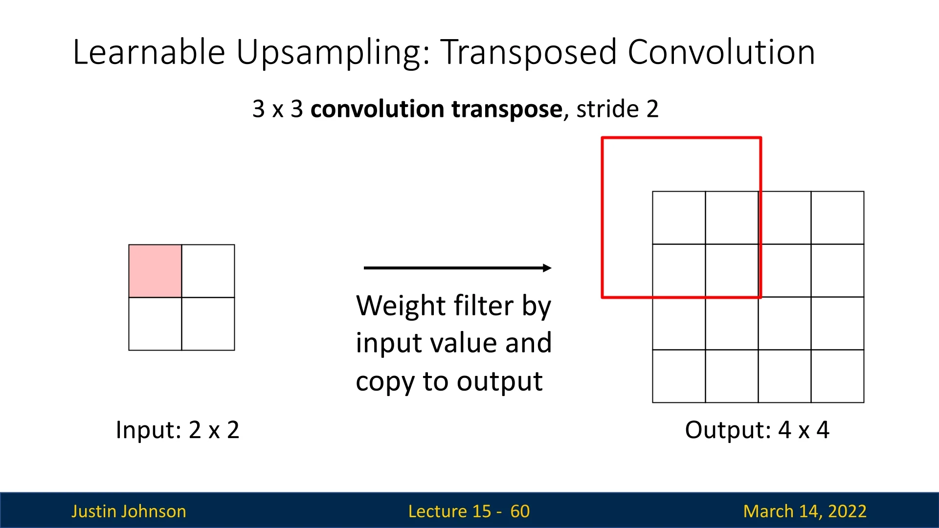
Step-by-Step Process of Transposed Convolution
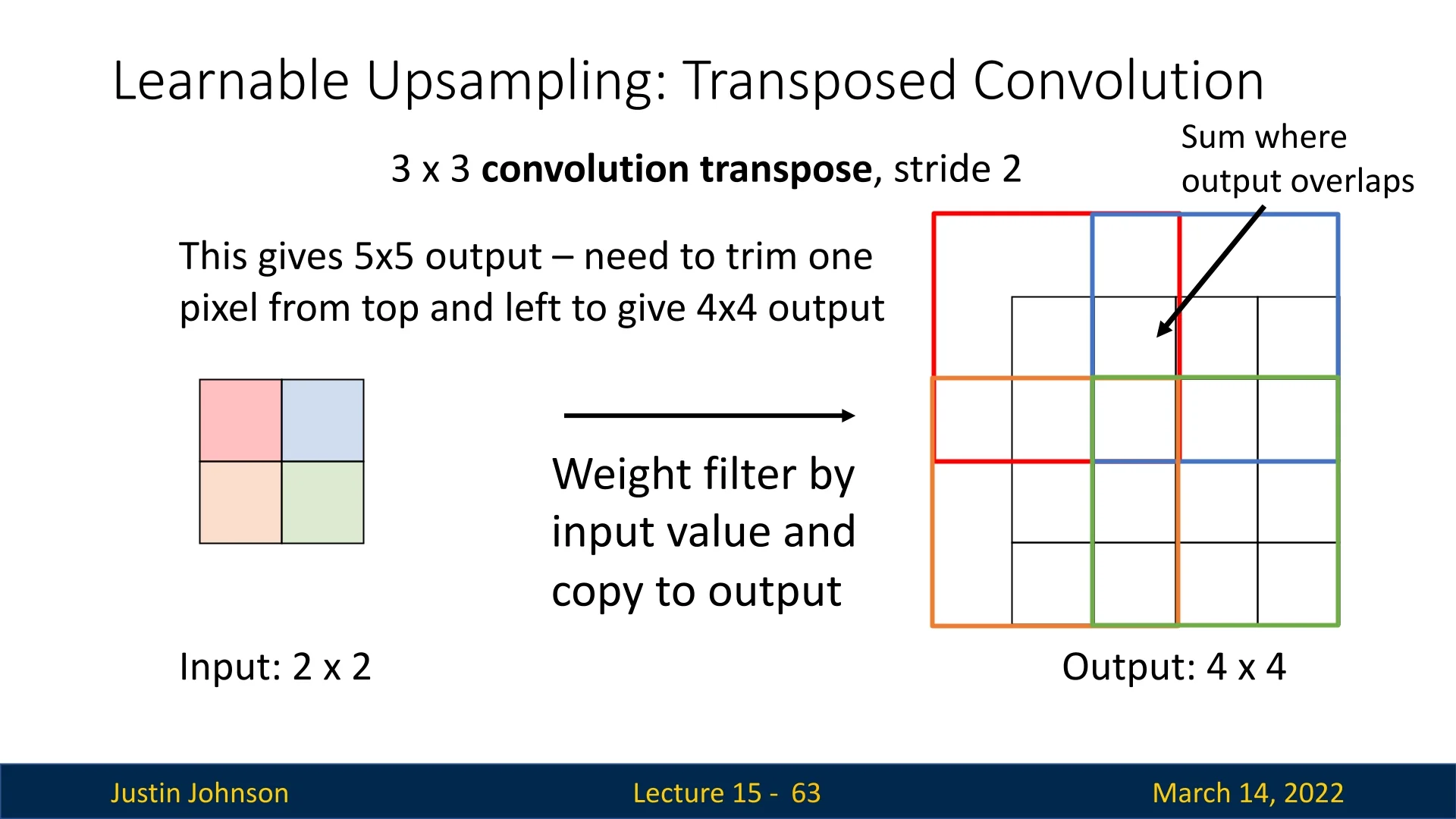
To illustrate how transposed convolution operates, consider a \(2 \times 2\) input feature map processed with a \(3 \times 3\) filter and a stride of 2, producing a \(4 \times 4\) output. The process consists of the following steps:
- 1.
- Processing the First Element:
- The first input value is multiplied element-wise with each value in the \(3 \times 3\) filter.
- The weighted filter response is then placed into its corresponding region in the output tensor, which was initially set to zeros.
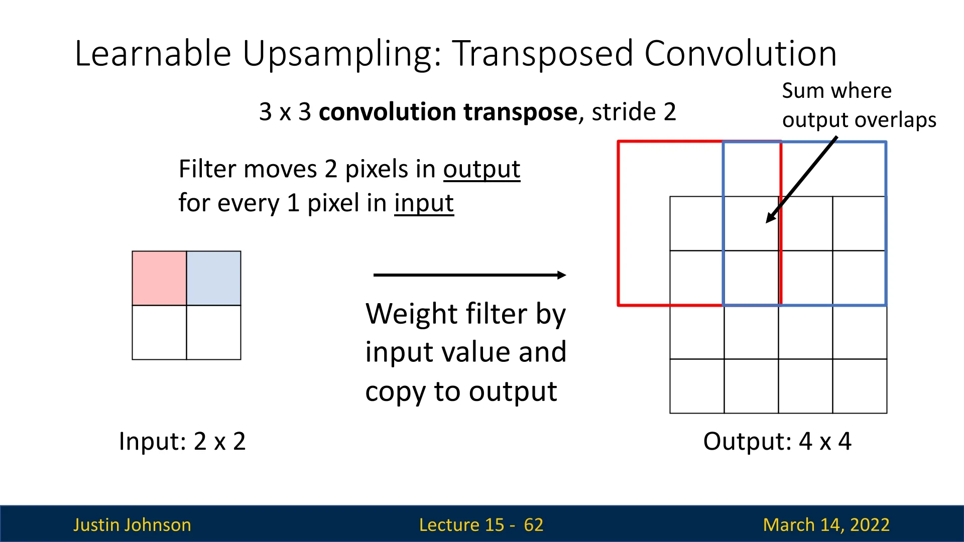
- 2.
- Processing the Second Element:
- The second input element undergoes the same multiplication with the filter, producing another set of weighted values.
- These values are positioned in the output grid according to the stride of 2.
- When regions of the output overlap due to filter applications, the corresponding values are summed instead of overwritten.
- 3.
- Iterating Over the Remaining Elements:
- The process is repeated for all input elements, progressively constructing the upsampled feature map.
- The final reconstructed output is a \(4 \times 4\) feature map, demonstrating how transposed convolution expands spatial resolution while preserving learned feature relationships.
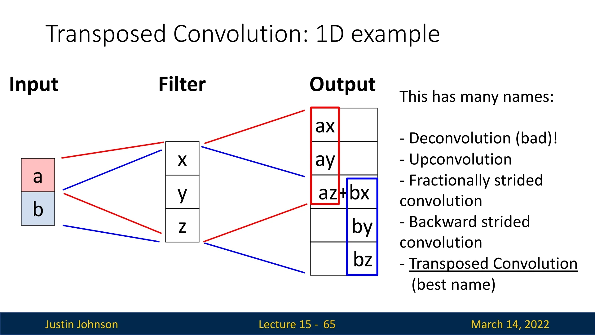
1D Transposed Convolution
A particularly clear way to build intuition for transposed convolution is to start from a simple 1D example and view it as a “scale, place, and sum” operation. Consider a transposed convolution that maps a 2-element input to a 5-element output using a 3-element kernel with stride \(S = 2\) and no padding.
- Input: \(\mathbf {u} = [a,\, b]^\top \)
- Kernel (filter): \(\mathbf {k} = [x,\, y,\, z]^\top \)
- Output: \(\mathbf {v} \in \mathbb {R}^5\)
The forward computation can be understood in three steps:
1. Scale and place each input element For each input element, we multiply the entire kernel and place the resulting block into the output at a location determined by the stride \(S\).
- For the first input \(a\), we form \[ a \cdot [x, y, z] = [ax,\, ay,\, az], \] and place it starting at the first output position: \[ [ax,\, ay,\, az,\, 0,\, 0]. \]
- For the second input \(b\), we again form \[ b \cdot [x, y, z] = [bx,\, by,\, bz], \] but now place it shifted by the stride \(S = 2\). This means its first element aligns with the third output position: \[ [0,\, 0,\, bx,\, by,\, bz]. \]
2. Sum overlapping contributions The final output \(\mathbf {v}\) is the elementwise sum of these placed blocks: \[ \mathbf {v} = \underbrace {[ax,\, ay,\, az,\, 0,\, 0]}_{\mbox{from } a} + \underbrace {[0,\, 0,\, bx,\, by,\, bz]}_{\mbox{from } b} = [ax,\, ay,\, az + bx,\, by,\, bz]^\top . \] The third position receives contributions from both \(a\) and \(b\), illustrating how transposed convolution blends neighboring inputs via overlapping kernel footprints.
3. Why 5 output elements? Role of stride The output length is determined by the standard 1D transposed convolution formula (no padding): \[ N_{\mbox{out}} = S \cdot (N_{\mbox{in}} - 1) + K, \] where \(N_{\mbox{in}} = 2\) (input length), \(K = 3\) (kernel size), \(S = 2\) (stride). Thus, \[ N_{\mbox{out}} = 2 \cdot (2 - 1) + 3 = 5. \] Intuitively, stride \(S = 2\) means that the two kernel “footprints” are placed two positions apart in the output, and each footprint spans \(K = 3\) elements, causing them to overlap in the middle.
In higher dimensions (e.g., 2D feature maps), exactly the same mechanism applies: each activation spreads its influence over a local neighborhood, shifted according to the stride, and overlapping contributions are summed to produce a larger, learned upsampled feature map.
Why use stride \(S>1\) in transposed convolutions? In practice, choosing a stride \(S>1\) in a transposed convolution is precisely how we perform learnable upsampling in a single layer. For a transposed convolution with stride \(S\), kernel size \(K\), padding \(P\), and 1D input length \(I\), \[ O = (I - 1)\cdot S + K - 2P \] controls the output size. For example, \(S=2\) approximately doubles the spatial resolution, and \(S=4\) approximately quadruples it (up to boundary effects). This is why decoder architectures for semantic segmentation (e.g., U-Net, FCN-style models) or generators in GANs and super-resolution networks routinely use stride-2 (or larger) transposed convolutions: they efficiently map low-resolution feature maps back to higher resolutions while learning how information should be distributed into the new pixels. Implementation-wise, a stride-\(S\) transposed convolution is equivalent to inserting \(S-1\) zeros between input positions and then applying a stride-1 convolution with the same kernel, but deep learning libraries realize this without explicitly constructing the enlarged, sparse intermediate tensor.
15.3.7 Convolution and Transposed Convolution as Matrix Multiplication
Convolutions are linear operations and can always be written as matrix–vector products. This viewpoint is useful conceptually (it shows that convolution is just a special sparse linear map) and practically (it explains why the forward pass of a transposed convolution corresponds to multiplying by the transpose of the convolution matrix, and why the backward pass of a standard convolution looks like a transposed convolution).
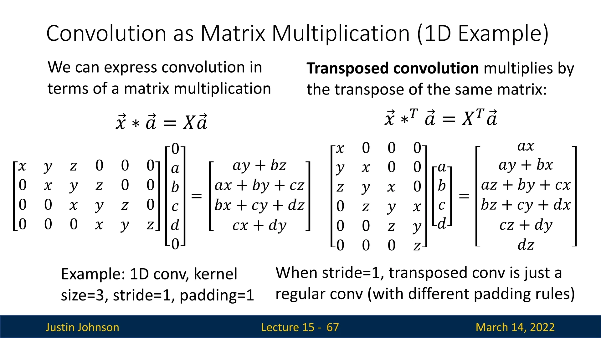
Standard Convolution via Matrix Multiplication
Consider a 1D convolution with stride \(S=1\) and no padding. Let
- Input: \(\mathbf {x} = [x_1, x_2, x_3, x_4]^\top \in \mathbb {R}^{4}\).
- Kernel (filter): \(\mathbf {w} = [w_1, w_2, w_3]^\top \in \mathbb {R}^{3}\).
With valid convolution, the output has length \[ O = I - K + 1 = 4 - 3 + 1 = 2, \] and its entries are \[ y_1 = w_1 x_1 + w_2 x_2 + w_3 x_3, \qquad y_2 = w_1 x_2 + w_2 x_3 + w_3 x_4. \]
We can write this as a matrix–vector product \[ \mathbf {y} = C \mathbf {x}, \] where \(C \in \mathbb {R}^{2 \times 4}\) is a Toeplitz matrix constructed from the kernel: \[ C = \begin {bmatrix} w_1 & w_2 & w_3 & 0 \\ 0 & w_1 & w_2 & w_3 \end {bmatrix}. \] Then \[ C \mathbf {x} = \begin {bmatrix} w_1 & w_2 & w_3 & 0 \\ 0 & w_1 & w_2 & w_3 \end {bmatrix} \begin {bmatrix} x_1 \\ x_2 \\ x_3 \\ x_4 \end {bmatrix} = \begin {bmatrix} w_1 x_1 + w_2 x_2 + w_3 x_3 \\ w_1 x_2 + w_2 x_3 + w_3 x_4 \end {bmatrix}, \] which matches the convolution exactly.
Each row of \(C\) encodes one position of the sliding kernel:
- Row 1 aligns \([w_1, w_2, w_3]\) with \([x_1, x_2, x_3]\).
- Row 2 shifts this pattern one step to the right, aligning with \([x_2, x_3, x_4]\).
Positions that would fall outside the input are filled with zeros. In higher dimensions (2D images, 3D volumes) and with multiple channels, the same idea produces larger, block-structured Toeplitz matrices.
Stride \(S>1\) in standard convolution For stride \(S>1\), the convolution still has the form \(\mathbf {y} = C_S \mathbf {x}\) for a suitable sparse matrix \(C_S\). Intuitively, the kernel still slides along the input, but we only keep every \(S\)-th output. In matrix form, this corresponds either to:
- Taking a subset of rows from the stride-1 Toeplitz matrix.
- Directly constructing a sparser matrix \(C_S\) whose rows correspond to windows starting at positions \[ 1,\; 1 + S,\; 1 + 2S,\; \dots \] in the input.
Transposed Convolution as the Matrix Transpose
The transposed convolution associated with a given (discrete) convolution is most cleanly defined via the transpose of its convolution matrix. If a standard 1D convolution with stride \(S\) can be written as \[ \mathbf {y} = C_S \mathbf {x}, \] then its associated transposed convolution is the linear map \[ \mathbf {x}' = C_S^\top \mathbf {y}. \] When \(C_S\) corresponds to a downsampling convolution (e.g., \(S > 1\)), this adjoint map typically increases spatial extent, which is why transposed convolutions are used for upsampling.
For the stride-\(1\) example above, the convolution matrix is \[ C = \begin {bmatrix} w_1 & w_2 & w_3 & 0 \\ 0 & w_1 & w_2 & w_3 \end {bmatrix} \in \mathbb {R}^{2 \times 4}, \] so its transpose is \[ C^\top = \begin {bmatrix} w_1 & 0 \\ w_2 & w_1 \\ w_3 & w_2 \\ 0 & w_3 \end {bmatrix} \in \mathbb {R}^{4 \times 2}. \] Given \(\mathbf {y} = [y_1, y_2]^\top \), the transposed convolution computes \[ \mathbf {x}' = C^\top \mathbf {y} = \begin {bmatrix} w_1 y_1 \\ w_2 y_1 + w_1 y_2 \\ w_3 y_1 + w_2 y_2 \\ w_3 y_2 \end {bmatrix}. \] Each element of \(\mathbf {y}\) is “spread” over three positions in \(\mathbf {x}'\), weighted by the kernel, and overlapping contributions are summed. For \(S=1\), both \(C\) and \(C^\top \) are Toeplitz matrices, so the adjoint is itself a normal convolution (with a flipped kernel).
Relating to the \([a, b]^\top \) and \([x, y, z]^\top \) Example (Stride \(S=2\))
We now connect the intuitive scale–place–sum example to the matrix view for stride \(S=2\). Consider a standard 1D convolution with:
- Input: \(\mathbf {v} = [v_1, v_2, v_3, v_4, v_5]^\top \).
- Kernel: \(\mathbf {k} = [x, y, z]^\top \).
- Stride: \(S = 2\), no padding.
The output \(\mathbf {u} = [u_1, u_2]^\top \) is \[ u_1 = x v_1 + y v_2 + z v_3, \qquad u_2 = x v_3 + y v_4 + z v_5, \] so the convolution matrix \(W \in \mathbb {R}^{2 \times 5}\) is \[ W = \begin {bmatrix} x & y & z & 0 & 0 \\ 0 & 0 & x & y & z \end {bmatrix}. \] Each row corresponds to placing the kernel at positions \((1,2,3)\) and \((3,4,5)\) in the input, reflecting the stride \(S=2\).
The associated transposed convolution uses \(W^\top \): \[ W^\top = \begin {bmatrix} x & 0 \\ y & 0 \\ z & x \\ 0 & y \\ 0 & z \end {bmatrix} \in \mathbb {R}^{5 \times 2}. \] Given a 2-element input \(\mathbf {u} = [a, b]^\top \), the transposed convolution computes \[ \mathbf {v}' = W^\top \mathbf {u} = a \begin {bmatrix} x \\ y \\ z \\ 0 \\ 0 \end {bmatrix} + b \begin {bmatrix} 0 \\ 0 \\ x \\ y \\ z \end {bmatrix} = \begin {bmatrix} ax \\ ay \\ az + bx \\ by \\ bz \end {bmatrix}. \] Thus the mapping \[ [a, b]^\top \;\xrightarrow {\;\mbox{kernel }[x,y,z]^\top ,\; S=2\;} [ax,\, ay,\, az+bx,\, by,\, bz]^\top \] is exactly the same 1D transposed convolution we described earlier, now written as a single matrix–vector product \(\mathbf {v}' = W^\top \mathbf {u}\).
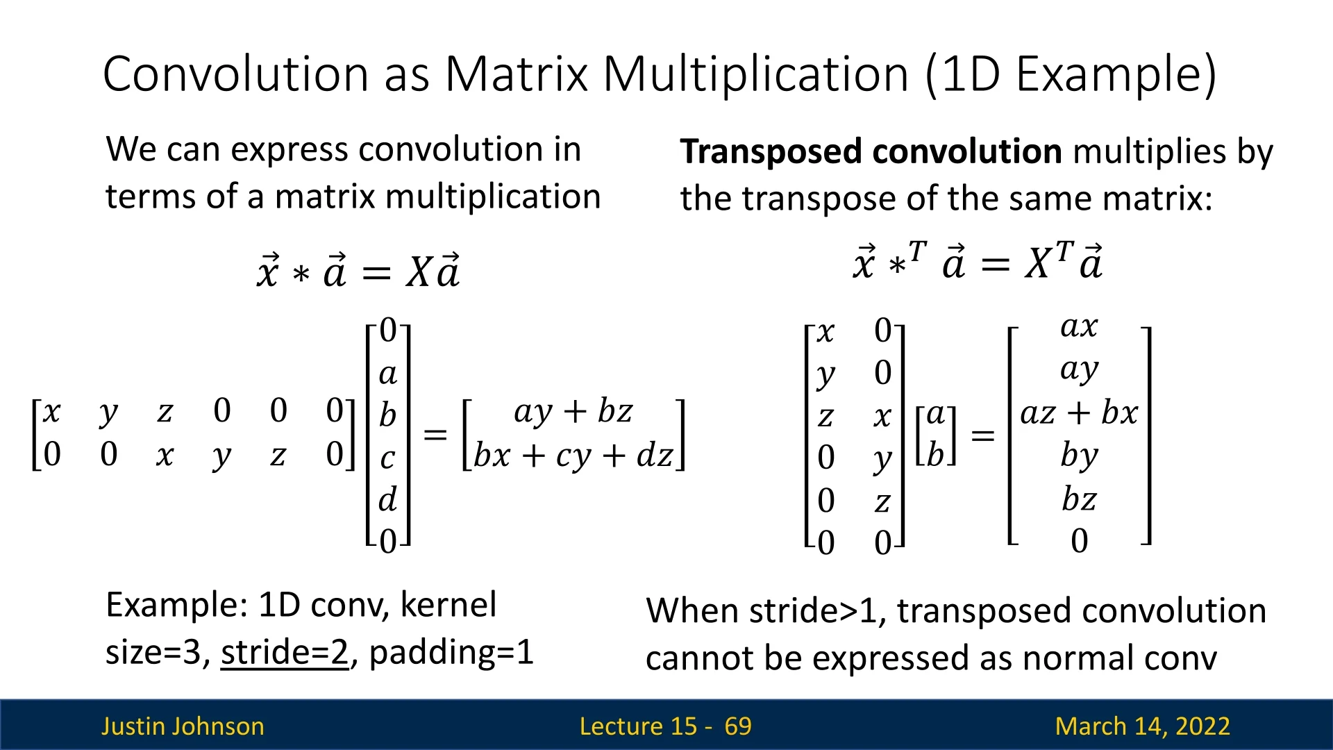
Strides, Upsampling, and the “Normal Convolution” Caveat
The matrix viewpoint is completely general: for any stride \(S\), both convolution and its adjoint remain linear maps and can always be written as \[ \mathbf {y} = C_S \mathbf {x}, \qquad \mathbf {x}' = C_S^\top \mathbf {y}, \] for some (possibly large and sparse) matrix \(C_S\). This makes it clear that:
- The operations are differentiable everywhere, with Jacobians given by \(C_S\) and \(C_S^\top \).
- Gradients with respect to inputs and kernels are just matrix–vector products involving these matrices or their transposes.
However, there is an important subtlety when \(S>1\):
- For \(\boldsymbol {S=1}\), the convolution matrix \(C\) is Toeplitz, and its transpose \(C^\top \) is also Toeplitz. In this case, both the forward convolution \(\mathbf {y} = C \mathbf {x}\) and the adjoint \(\mathbf {x}' = C^\top \mathbf {y}\) are normal convolutions on the same grid, with different (flipped) kernels.
- For \(\boldsymbol {S>1}\), the forward convolution matrix \(C_S\) is still Toeplitz (up to zero rows corresponding to skipped positions), but its transpose \(C_S^\top \) is no longer Toeplitz. As the stride example above shows, \(W^\top \) does not have constant diagonals, so there is no single kernel and stride configuration that realizes \(\mathbf {x}' = C_S^\top \mathbf {y}\) as a single standard convolution on the original input grid.
This is precisely the sense in which, for \(S>1\), a transposed convolution cannot be expressed as a normal convolution acting directly on \(\mathbf {y}\): its matrix is not a convolution (Toeplitz) matrix on that grid. Instead, the usual implementation factorizes the operation into two steps:
- 1.
- Zero-insertion (upsampling). Conceptually insert \(S-1\) zeros between consecutive elements of \(\mathbf {y}\), creating an enlarged, sparse feature map.
- 2.
- Stride-1 convolution. Apply a normal stride-1 convolution (with an appropriate kernel) to this upsampled signal.
On the upsampled grid, the second step is again a standard convolution with a Toeplitz matrix. But on the original grid, the full operator is no longer a single convolution; it is the composition of upsampling (a fixed linear map) and a stride-1 convolution. Deep learning libraries implement transposed convolutions in exactly this way for efficiency, rather than explicitly forming \(C_S^\top \).
In summary:
- Mathematically, for any stride \(S\), convolution and transposed convolution are linear maps with an adjoint relationship \(\mathbf {y} = C_S \mathbf {x}\), \(\mathbf {x}' = C_S^\top \mathbf {y}\).
- For \(S=1\), both maps are themselves normal convolutions on the same grid.
- For \(S>1\), the adjoint \(C_S^\top \) is not a normal convolution on the original grid, but can be implemented as “upsample (insert zeros) + stride-1 convolution” on a finer grid.
This clarifies why transposed convolutions with stride \(S>1\) are treated as a distinct primitive in modern libraries, even though they are still fully linear and differentiable and remain the exact adjoints of their corresponding strided convolutions.
Advantages of Transposed Convolution
Relative to fixed upsampling operations such as bilinear interpolation or max unpooling, transposed convolution offers several advantages:
- Learnable weights: The kernel parameters are trained end-to-end, allowing the network to learn how best to interpolate and refine details for the specific task.
- Trainable spatial structure: Because it is a convolution, the operation naturally captures local spatial patterns and can reconstruct sharp edges and meaningful structures rather than merely smoothing.
- Flexible stride and padding: As with standard convolutions, stride, kernel size, and padding provide fine-grained control over the output resolution, making it easy to design multi-scale encoder–decoder architectures.
Challenges and Considerations
While transposed convolution is highly effective, it introduces some challenges:
- Checkerboard Artifacts: Overlapping filter applications can create unevenly distributed activations, leading to artifacts in the output.
- Sensitivity to Stride and Padding: Incorrect configurations can lead to distorted feature maps or excessive upsampling.
15.3.8 Conclusion: Choosing the Right Upsampling Method
In this chapter we examined several upsampling and unpooling strategies, ranging from simple, non-learnable schemes to fully learnable transposed convolutions. Each method makes a different trade-off between computational cost, spatial faithfulness, smoothness, and the ability to recover or hallucinate fine details. In practice, the “right” choice depends on the task (e.g., semantic segmentation vs. super-resolution), the downsampling operations used in the encoder (max pooling vs. strided convolutions), and the amount of computation and complexity you are willing to invest in the decoder.
| Upsampling Method | Advantages | Limitations |
|---|---|---|
| Nearest-Neighbor Unpooling / Upsampling | Extremely simple and fast; no learnable parameters; preserves exact values of input pixels or features | Produces blocky, jagged artifacts; no notion of continuity; cannot reconstruct fine details or smooth transitions. |
| Bed of Nails Unpooling | Simple non-learnable unpooling; preserves original values in fixed locations; keeps sparsity structure | Places activations in arbitrary fixed positions (e.g., always top-left); breaks spatial alignment with the encoder; creates unnatural gaps and aliasing; generally inferior to max unpooling. |
| Bilinear Interpolation | Fast, differentiable, and easy to implement; produces smooth transitions and avoids blocky artifacts | Averages over local neighborhoods, which blurs edges and textures; cannot recover high-frequency details lost during downsampling. |
| Bicubic Interpolation | Uses a larger neighborhood and cubic weights; typically sharper outputs and better detail preservation than bilinear | More computationally expensive; still non-learnable and can introduce mild blurring or ringing near sharp boundaries. |
| Max Unpooling | Restores activations to their exact locations recorded by max pooling; preserves spatial layout of salient features and encoder–decoder alignment | Produces sparse feature maps (zeros in non-max positions) that require subsequent convolutions for refinement; only applicable when pooling indices are available. |
| Transposed Convolution | Fully learnable upsampling; can reconstruct or hallucinate high-frequency structure; flexible control of output size through kernel, stride, and padding | Higher computational cost; can introduce checkerboard artifacts if kernel size, stride, and padding are poorly chosen; more sensitive to implementation details. |
Guidelines for Choosing an Upsampling Method
The upsampling strategy should be chosen in concert with the encoder design and the target task. The following guidelines capture common patterns used in practice:
-
Match the encoder’s downsampling when using max pooling.
When the encoder uses max pooling, max unpooling is a natural counterpart: it reuses the recorded pooling indices to place activations back into their original spatial locations. This preserves spatial correspondence between encoder and decoder feature maps.Because the unpooled output is sparse, it should almost always be followed by one or more convolutional layers to “densify” and refine the feature map. In contrast, Bed of Nails unpooling does not respect the original pooling geometry and typically leads to misaligned features and artifacts, so it is best viewed as a simple didactic baseline rather than a practical choice.
- Use interpolation when you want smooth, non-learnable
upsampling.
For tasks where smoothness and simplicity are more important than exact detail reconstruction (or when a lightweight baseline is sufficient), bilinear interpolation is a robust default. It avoids blocky artifacts and is inexpensive. Bicubic interpolation is preferred when additional sharpness is desired and the extra cost is acceptable. In both cases, the upsampled features are often followed by a standard convolution layer to reintroduce some learnable flexibility. - Combine simple upsampling with convolution to avoid
artifacts.
A widely used pattern in modern architectures is: resize (nearest-neighbor or bilinear) \(\rightarrow \) convolution. The interpolation step handles the geometric upsampling, while the subsequent convolution learns to refine and reweight the features. This decoupled design avoids checkerboard artifacts associated with poorly configured transposed convolutions, yet retains learnable capacity through the convolutional layer. - Use transposed convolution when learnable upsampling is
essential.
Transposed convolutions are often preferred in semantic segmentation decoders, autoencoders, super-resolution networks, and GAN generators, where the decoder must learn how to reconstruct or hallucinate fine details from compact representations. By choosing appropriate kernel sizes and strides (e.g., even kernel sizes and strides that match the encoder’s downsampling pattern), transposed convolutions can provide powerful, learnable upsampling. Careful design or additional smoothing (e.g., a small convolution after the transposed convolution) is recommended to mitigate checkerboard artifacts. - For encoders without explicit pooling, favor learned,
structured upsampling.
In fully convolutional architectures that rely primarily on strided convolutions for downsampling, there are no pooling indices to reuse. In such cases, transposed convolutions or interpolation + convolution blocks provide a natural way to invert the spatial contraction, since they can be configured to mirror the encoder’s stride pattern and learn how to reconstruct structured high-resolution outputs.
In summary, nearest-neighbor and Bed of Nails unpooling serve as simple baselines, interpolation methods provide smooth but non-learnable upsampling, and max unpooling plus transposed convolutions exploit encoder information or learnable filters to recover structure. Most practical decoders combine these ideas—using indices when available, interpolation when stability and simplicity matter, and learnable convolutions when detailed reconstruction is crucial.
15.5 Instance Segmentation
Instance segmentation is a critical task in computer vision that aims to simultaneously detect and delineate each object instance within an image. Unlike semantic segmentation, which assigns a class label to each pixel without distinguishing between different object instances of the same category, instance segmentation uniquely identifies each occurrence of an object. This is particularly important for applications where individual object identification is required, such as autonomous driving, medical imaging, and robotics.
In computer vision research, image regions are categorized into two types: things and stuff. This distinction is fundamental to instance segmentation, where individual object instances are identified at the pixel level.
- Things: Object categories that can be distinctly separated into individual instances, such as cars, people, and animals.
- Stuff: Object categories that lack clear instance boundaries, such as sky, grass, water, and road surfaces.
Instance segmentation focuses exclusively on things, as segmenting instances of stuff is not meaningful. The primary goal of instance segmentation is to detect all objects in an image and assign a unique segmentation mask to each detected object, ensuring correct differentiation of overlapping instances.
This task is particularly challenging due to the need for accurate pixel-wise delineation while simultaneously handling object occlusions, varying scales, and complex background clutter. Advanced deep learning architectures, such as Mask R-CNN, have significantly improved the performance of instance segmentation by leveraging region-based feature extraction and mask prediction techniques.
The development of instance segmentation models continues to evolve, driven by the increasing demand for high-precision vision systems across various domains.
15.4.1 Mask R-CNN: A Two-Stage Framework for Instance Segmentation
Mask R-CNN extends Faster R-CNN, a widely used two-stage object detection framework, by incorporating a dedicated branch for per-instance segmentation masks. While Faster R-CNN predicts bounding boxes and class labels, Mask R-CNN further refines this process by generating high-resolution segmentation masks for each detected object.
Faster R-CNN Backbone
Faster R-CNN builds on a convolutional backbone (e.g., ResNet with or without FPN) that extracts a shared feature map for the entire image. On top of these features, a Region Proposal Network (RPN) predicts a set of candidate object bounding boxes (region proposals) together with objectness scores. For each proposal, features are cropped from the shared feature map (via RoI pooling or RoI Align) and passed through two parallel heads: a classification head that predicts the object category via softmax, and a bounding box regression head that refines the proposal coordinates via regression. This two-stage design yields class-labeled, refined bounding boxes and serves as the foundation for Mask R-CNN.
Key Additions in Mask R-CNN
Mask R-CNN preserves the overall Faster R-CNN structure while introducing two key modifications that enable instance-level segmentation:
-
A mask prediction head. A lightweight fully convolutional network (FCN) branch predicts a binary segmentation mask for each detected object instance. Instead of producing a single segmentation map for the whole image, Mask R-CNN outputs one mask per region of interest (RoI). The mask head consists of several convolutional layers followed by a deconvolution (transposed convolution) layer that upsamples RoI features (e.g., from \(14 \times 14\) to \(28 \times 28\)) before a final \(1 \times 1\) convolution produces per-pixel mask logits. The weights of this head are learned jointly with the detection heads.
- RoI Align for precise feature extraction. Faster R-CNN originally used RoI Pooling, which quantizes RoI coordinates to discrete bins and introduces misalignment between the RoI and the underlying feature map. Mask R-CNN replaces this with RoI Align, which avoids any rounding and uses bilinear interpolation to sample feature values at exact (possibly fractional) locations. This improves alignment, especially for small objects, and is crucial for accurate mask boundaries.
As a result, the second stage of Mask R-CNN produces three parallel outputs for each region proposal:
- Class label, predicted via a softmax classification head.
- Bounding box refinement, predicted by a regression head that outputs coordinate offsets.
- Segmentation mask, predicted by the FCN-based mask branch.
Segmentation Mask Prediction: Fixed-Size Output
A central challenge in instance segmentation is handling objects of widely varying sizes while keeping computation manageable. Mask R-CNN addresses this by predicting a fixed-size mask for each RoI and then resizing it to the object’s bounding box in the original image.
Concretely, for each positive RoI:
- 1.
- The RPN generates region proposals on top of the backbone feature map.
- 2.
- The classification and bounding box regression heads operate on RoI-aligned features to predict the object category and refine the bounding box coordinates.
- 3.
- In parallel, the mask head takes the same RoI-aligned features and outputs a tensor of shape \(C \times 28 \times 28\), where \(C\) is the number of object classes. Each channel corresponds to a class-specific mask prediction at a fixed spatial resolution.
- 4.
- During inference, the mask corresponding to the predicted class for that RoI is selected, yielding a single \(28 \times 28\) mask for that instance.
- 5.
- This selected \(28 \times 28\) mask is then resized to the spatial extent of the refined bounding box using bilinear interpolation and placed at the appropriate location in the original image coordinate system.
In other words, the transposed convolution inside the mask head learns to produce a relatively high-resolution, fixed-size mask in feature space, while a final bilinear interpolation step adapts this fixed-size mask to the object’s actual size in the input image.
Training Mask R-CNN and Loss Functions
Mask R-CNN is trained end-to-end as a multi-task model, jointly optimizing detection (classification and bounding boxes) and segmentation. The training objective is the sum of three losses:
- Classification loss \(L_{cls}\). A standard softmax cross-entropy loss applied to the classification head to encourage correct object category predictions for each RoI.
- Bounding box regression loss \(L_{box}\). A smooth L1 loss applied to the predicted bounding box offsets for positive RoIs (those that sufficiently overlap a ground-truth object), improving localization accuracy.
- Mask loss \(L_{mask}\). A per-pixel binary cross-entropy loss applied to the mask prediction branch. For each positive RoI, this loss is computed only on the channel corresponding to the ground-truth class, ignoring all other class channels. This class-specific loss encourages accurate foreground–background separation and precise object boundaries.
The total loss is given by \[ L = L_{cls} + L_{box} + L_{mask}, \] where:
- \(L_{cls}\) is the classification loss.
- \(L_{box}\) is the bounding box regression loss.
- \(L_{mask}\) is the mask prediction loss.
In practice, the backbone network (e.g., ResNet with or without FPN) is first pretrained on a large-scale image classification dataset such as ImageNet and then fine-tuned on an instance segmentation dataset such as COCO. During fine-tuning, gradients from all three heads (classification, box regression, and mask prediction) are backpropagated through the shared backbone and RPN. This joint optimization improves both detection (bounding box mAP) and segmentation (mask mAP), and the RoI Align plus mask head design enables accurate, high-resolution instance masks while reusing the mature Faster R-CNN detection pipeline.
Bilinear Interpolation vs. Bicubic Interpolation
The upsampling step in Mask R-CNN requires resizing segmentation masks to fit detected object regions. The authors chose bilinear interpolation over bicubic interpolation for the following reasons:
- Efficiency: Bilinear interpolation is computationally less expensive than bicubic interpolation, making it suitable for processing multiple objects per image.
- Minimal Accuracy Gains from Bicubic: Bicubic interpolation considers 16 neighboring pixels, while bilinear uses only 4. Given that Mask R-CNN’s masks are already low resolution (\(28 \times 28\)), bicubic interpolation does not provide significant accuracy improvements.
- Edge Preservation: Bicubic interpolation introduces additional smoothing, which can blur object boundaries. Bilinear interpolation maintains sharper mask edges, improving segmentation performance.
Class-Aware Mask Selection
Unlike traditional multi-class segmentation models, which predict a single mask covering all categories, Mask R-CNN follows a per-instance, per-class approach:
- The segmentation head predicts C binary masks per object, where \(C\) is the number of possible classes.
- The classification head determines the object’s category.
- The corresponding mask for the predicted category is selected and applied to the object.
This method decouples classification from segmentation, preventing class competition within the mask and improving segmentation accuracy.
Gradient Flow in Mask R-CNN
Mask R-CNN’s forward pass for mask prediction closely mirrors the backward pass of standard convolutional networks. Gradient computations are structured as follows:
- The classification and bounding box losses propagate through the detection pipeline, refining object proposals.
- The segmentation loss propagates gradients through the mask prediction branch, optimizing instance masks.
- RoI Align ensures spatial alignment, preventing gradient misalignment and improving mask accuracy.
Expressing these processes as matrix–vector operations clarifies how gradients flow through the network, aiding optimization and efficient deep learning framework implementation.
Summary
Mask R-CNN extends Faster R-CNN by introducing a per-region mask prediction branch and RoI Align for accurate feature extraction. The segmentation head predicts a fixed-size \(28 \times 28\) binary mask per object, which is then resized using bilinear interpolation. This approach allows for accurate instance segmentation while maintaining computational efficiency, making Mask R-CNN a dominant framework in object segmentation applications.
15.4.2 Extending the Object Detection Paradigm
Mask R-CNN introduced a paradigm in which object detection models can be extended to perform new vision tasks by adding task-specific prediction heads. This flexible approach has led to the development of new capabilities beyond instance segmentation, such as:
-
Keypoint Estimation: Mask R-CNN was further extended for human pose estimation by adding a keypoint detection head. This variation, sometimes called Mask R-CNN: Keypoints, predicts key locations such as joints in the human body, facilitating pose estimation.
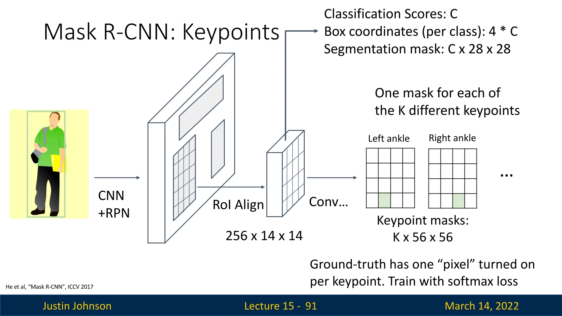
Figure 15.17: Mask R-CNN extended for keypoint estimation, predicting key locations such as joints for human pose estimation. -
Dense Captioning: Inspired by the Mask R-CNN paradigm, DenseCap [280] extends object detection by incorporating a captioning head. This approach, illustrated below, uses an LSTM-based captioning module to describe detected regions with natural language. We’ll cover this topic in depth later on.
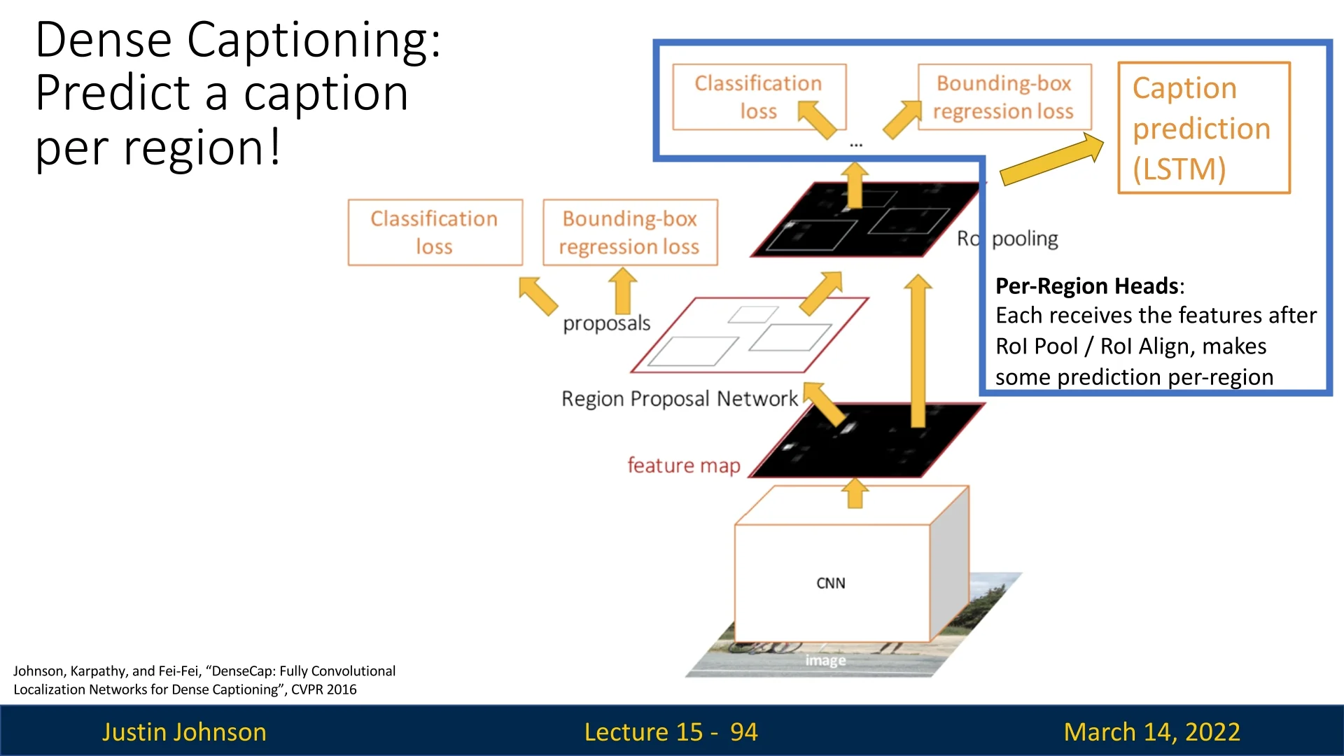
Figure 15.18: Dense Captioning (DenseCap) extends object detection by adding a captioning head, enabling textual descriptions of detected objects. 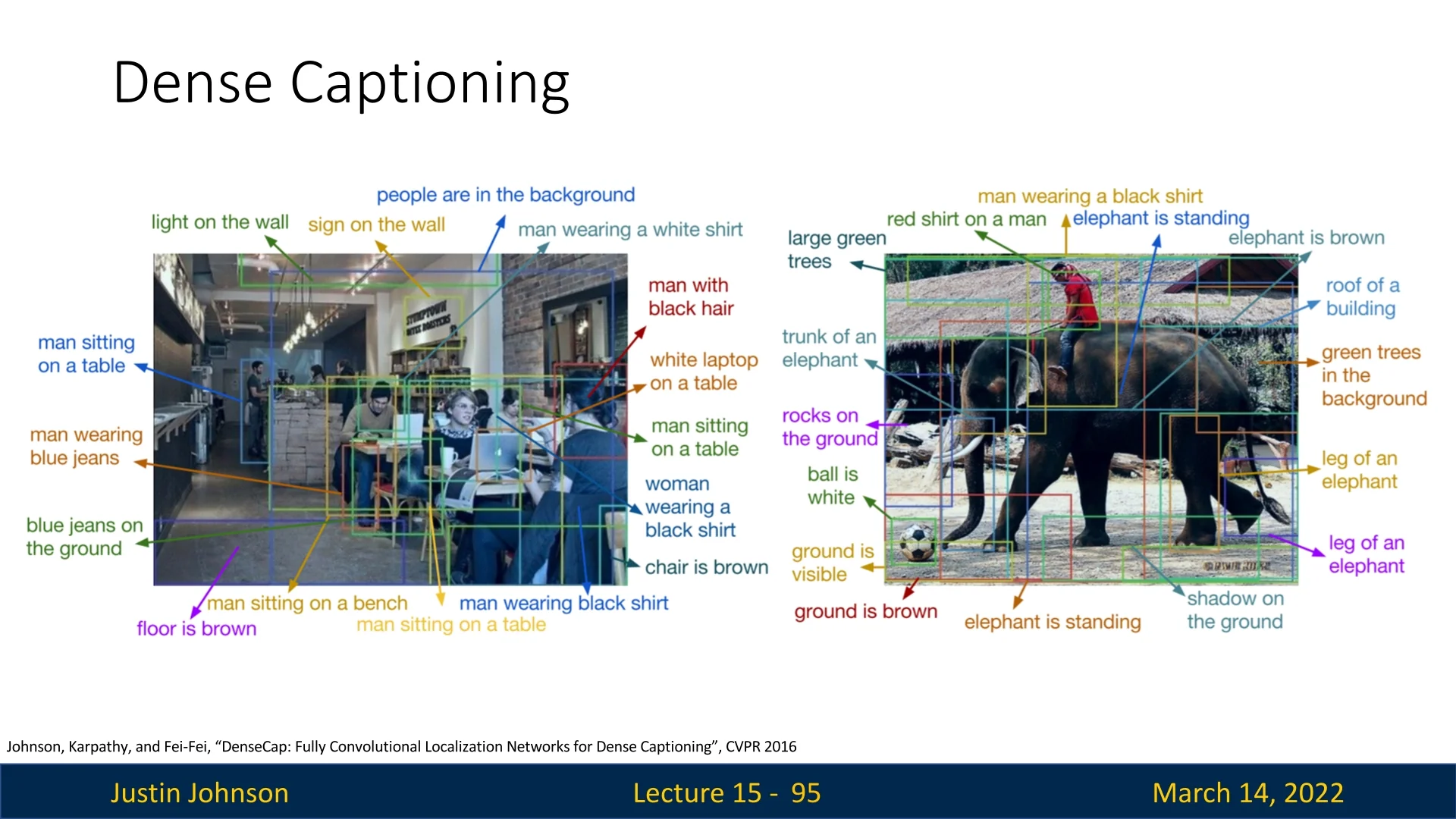
Figure 15.19: Example output of DenseCap: Generated captions describe detected regions with natural language. -
3D Shape Prediction: Mesh R-CNN [183] builds upon Mask R-CNN to predict 3D object shapes from 2D images by adding a mesh prediction head. This enables the reconstruction of 3D object geometry directly from image-based inputs, representing a significant step toward vision-based 3D reasoning.
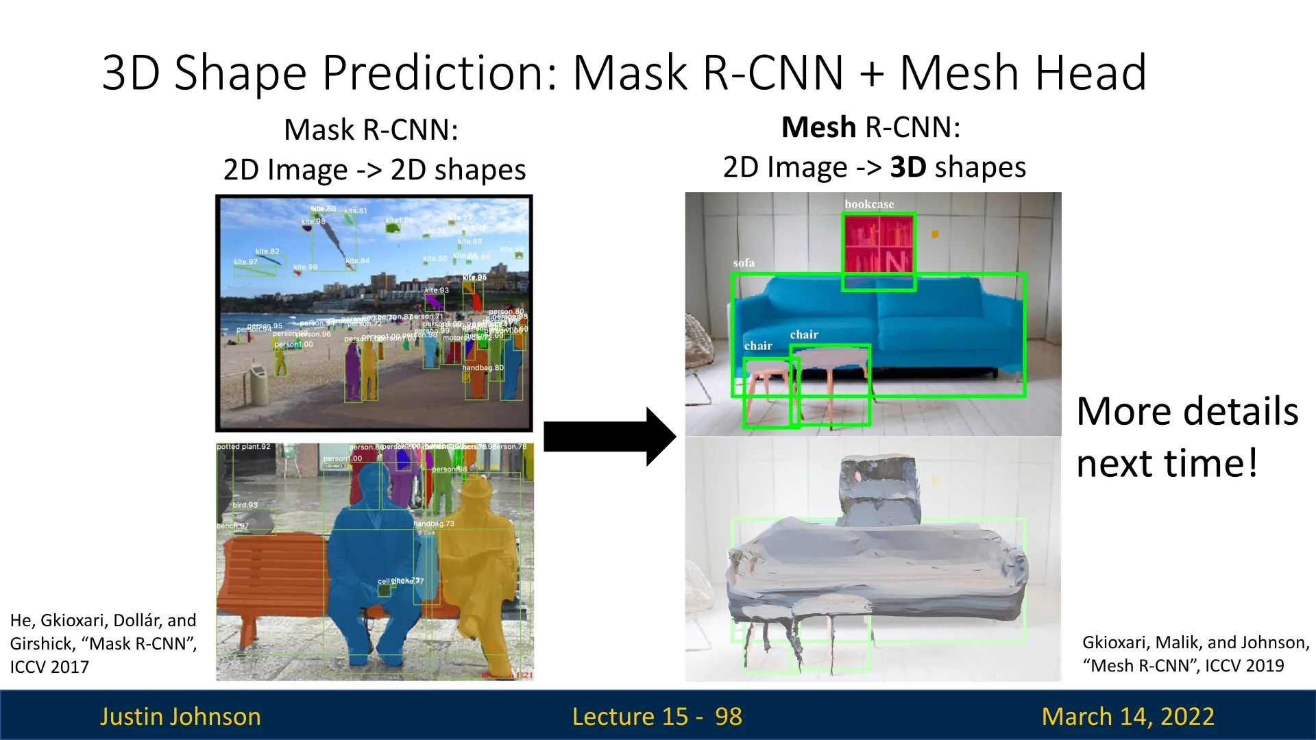
Figure 15.20: Mesh R-CNN extends Mask R-CNN with a mesh prediction head, enabling 3D shape reconstruction from 2D images.
These extensions highlight the versatility of the Mask R-CNN framework and demonstrate how object detection networks can serve as a foundation for diverse computer vision tasks. By incorporating additional task-specific heads, researchers continue to expand the boundaries of what can be achieved using a common underlying object detection architecture. We’ll touch these ideas later on as well.
Enrichment 15.6: U-Net: A Fully Conv Architecture for Segmentation
Enrichment 15.6.1: Overview
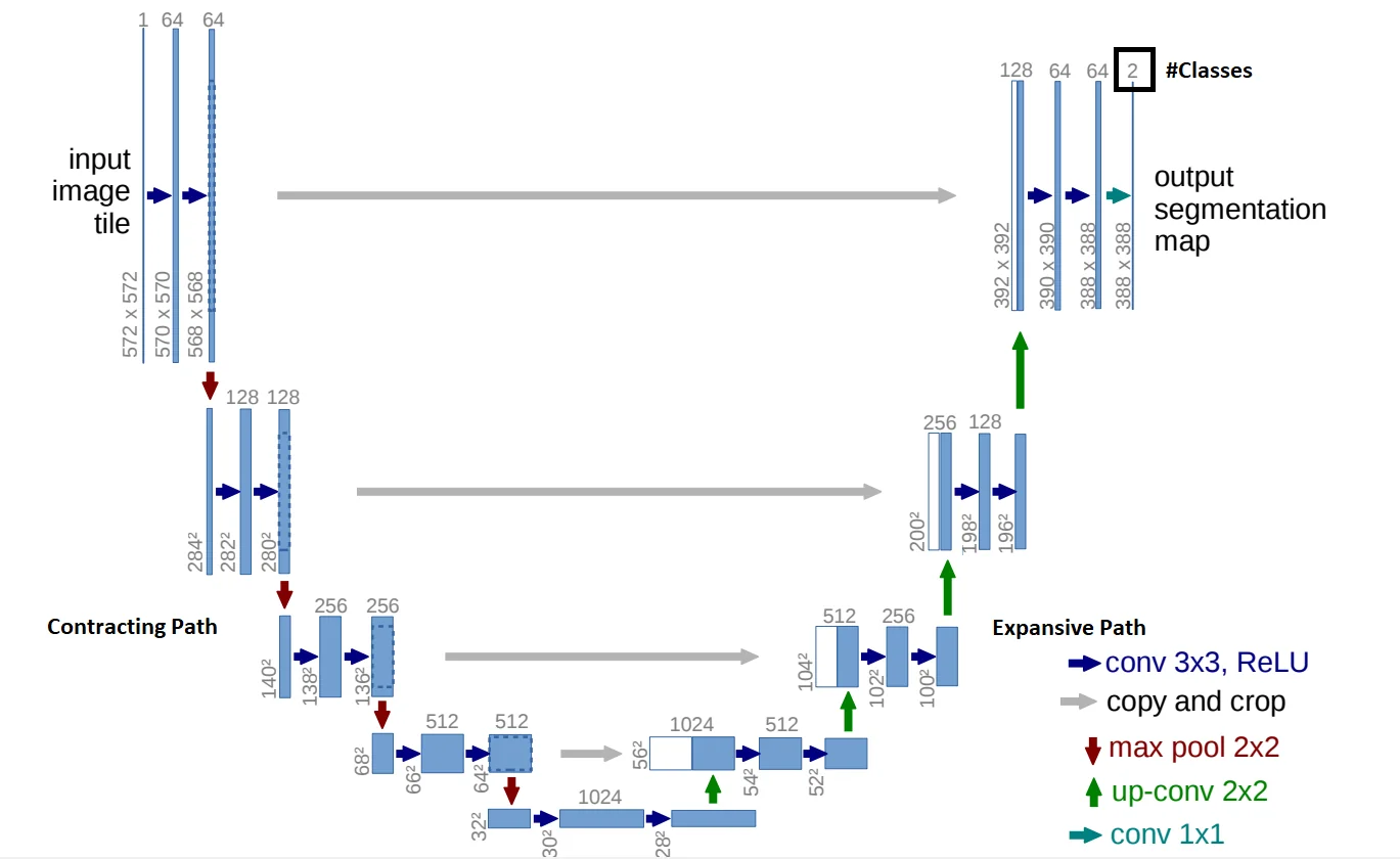
U-Net [549] is a fully convolutional neural network designed for semantic segmentation, particularly in biomedical imaging. Unlike traditional classification networks, U-Net assigns a class label to each pixel, performing dense prediction. The architecture follows a symmetrical encoder-decoder structure, resembling a ”U” shape. The encoder (contracting path) captures contextual information, while the decoder (expansive path) refines localization details.
Enrichment 15.6.2: U-Net Architecture
U-Net consists of two key components:
-
Contracting Path (Encoder):
- Repeated \(3 \times 3\) convolutions followed by ReLU activations.
- \(2 \times 2\) max-pooling for downsampling, reducing spatial resolution while increasing feature depth.
- Captures high-level semantic information necessary for object recognition.
-
Expansive Path (Decoder):
- Transposed convolutions for upsampling, restoring spatial resolution.
- Skip connections integrate feature maps from the encoder to retain spatial details lost during downsampling.
- A \(1 \times 1\) convolution maps feature channels to the segmentation classes.
Enrichment 15.6.3: Skip Connections and Concatenation
Skip connections are a key innovation in U-Net that directly link corresponding encoder and decoder layers through concatenation. This mechanism enables:
-
Preserving Spatial Information:
- Encoder feature maps are concatenated with decoder feature maps at corresponding levels.
- This ensures that fine-grained details lost due to downsampling are reinstated.
-
Combining Semantic and Spatial Features:
- The encoder extracts abstract, high-level semantic features.
- The decoder restores fine details, and concatenation helps merge these representations.
-
Enhancing Gradient Flow During Training:
- Skip connections allow gradients to propagate more easily through deep networks, preventing vanishing gradients.
- This improves convergence and stabilizes the training process.
The concatenation operation is crucial, as it ensures that both low-level spatial features and high-level semantic features contribute to final pixel-wise classification.
Enrichment 15.6.4: Training U-Net
U-Net is trained end-to-end in a supervised manner, typically using:
-
Loss Function:
- The standard loss function for U-Net is Binary Cross-Entropy (BCE) for binary segmentation tasks.
- For multi-class segmentation, Categorical Cross-Entropy is used.
- When dealing with imbalanced datasets, Dice Loss or a combination of BCE and Dice Loss is applied.
-
Optimization:
- U-Net is typically trained using Adam or Stochastic Gradient Descent (SGD) with momentum.
-
Data Augmentation:
-
Given the limited availability of annotated medical data, U-Net heavily relies on augmentation techniques such as:
- Random rotations, flips, and intensity shifts.
- Elastic deformations to improve robustness.
-
The combination of skip connections, effective loss functions, and augmentation techniques ensures that U-Net achieves high accuracy even with limited training data.
Enrichment 15.6.5: Comparison with Mask R-CNN
While both U-Net and Mask R-CNN perform segmentation, they differ in:
- Task Type: U-Net performs semantic segmentation; Mask R-CNN performs instance segmentation.
- Architecture: U-Net follows an encoder-decoder design, while Mask R-CNN uses a two-stage detection-segmentation approach.
- Application Domains: U-Net is dominant in medical imaging and satellite imagery, whereas Mask R-CNN excels in object detection and video analytics.
Enrichment 15.6.6: Impact and Evolution of U-Net
Since its introduction, U-Net has significantly influenced segmentation research, inspiring numerous adaptations and improvements:
- U-Net++ [822]: Incorporates dense connections between encoder-decoder layers to improve gradient flow and feature reuse.
- 3D U-Net [108]: Extends the architecture to volumetric data, benefiting applications like MRI and CT scan analysis.
- Residual U-Net [804]: Integrates residual blocks to enhance gradient flow and stabilize training for deeper architectures.
- Hybrid U-Net Variants: Many modern adaptations replace the convolutional backbone with newer architectures, such as vision transformers, to enhance feature extraction.
Although Attention U-Net [471] introduces an attention mechanism to selectively focus on relevant features, we have not yet covered attention mechanisms in this course. However, the core U-Net structure remains effective even without attention mechanisms and is widely used in practice. With continuous enhancements, U-Net’s impact on segmentation research persists across various domains.
Enrichment 15.7: Striding Towards SOTA Image Segmentation
Foundational segmentation systems By late 2025, modern segmentation has consolidated around two complementary families of models:
- Promptable foundation models (e.g., SAM, SAM 2, SAM 3) treat segmentation as answering queries about an image or video. Given sparse prompts—originally points, boxes, and masks, and now increasingly text and visual exemplars—they return high-quality masks, largely independent of any fixed label taxonomy.
- Universal task-trained transformers (e.g., Mask2Former, Mask DINO) treat segmentation as a closed-set prediction problem. They are trained on a fixed label space and directly output semantic, instance, or panoptic predictions for all categories in that taxonomy.
Our focus in this section is on the first family. Segment Anything (SAM) [309] reframed interactive segmentation as large-scale, promptable inference: given geometric hints (points, boxes, or a coarse mask), the model predicts the corresponding object mask, independent of category names. Its capabilities are driven both by a transformer-based encoder–decoder and by the SA-1B data engine, which couples model proposals with large-scale human correction to produce over one billion high-quality masks. Extending this idea from still images to videos, SAM 2 [529] adds a lightweight streaming memory that stores compact state across frames, enabling real-time propagation and interactive correction of masks over long videos; its data engine similarly scales from static images to large video corpora.
Most recently, SAM 3 [65] unifies this geometric precision with concept-level understanding. Instead of relying on external detectors for text prompts (as in Grounding DINO \(\to \) SAM-style pipelines), SAM 3 natively supports concept prompts: short noun phrases (e.g., “yellow school bus”), image exemplars, or combinations of both. The corresponding task, termed Promptable Concept Segmentation (PCS), takes such prompts and returns segmentation masks and identities for all matching instances in images and videos. Architecturally, SAM 3 shares a vision backbone between an image-level detector and a memory-based video tracker, and introduces a presence head that decouples recognition (“is this concept present here?”) from localization, improving open-vocabulary detection and tracking. In the remainder of this subsection we will treat the SAM family (SAM, SAM 2, SAM 3) as canonical examples of promptable segmentation; later sections return to SAM 2 and SAM 3 in more architectural detail.
In parallel, a second line of work focuses on task-specific, closed-world performance. Universal transformers such as Mask2Former [100] and Mask DINO [340] (covered later in this chapter) are trained to jointly solve semantic, instance, and panoptic segmentation on a fixed label set (e.g., COCO, Cityscapes), typically achieving state-of-the-art mIoU/PQ when the deployment taxonomy matches the training one. Their outputs are directly aligned with benchmark metrics and do not require user prompts at inference time.
Text-grounded segmentation: composite vs native A third, closely related direction is text-grounded segmentation. Before SAM 3, open-vocabulary segmentation typically relied on composite pipelines. Systems such as Grounding DINO [384] or OWLv2 [445] first performed grounding—mapping text prompts to boxes and labels—and then SAM or SAM 2 converted those boxes or points into precise masks. This pattern, often referred to as Grounded SAM [540], explicitly splits the problem into two stages: (1) a vision–language detector for text-to-box grounding, and (2) a promptable segmenter for box-to-mask refinement.
Conceptually, this brings us full circle to the two-stage design of classical detectors such as Mask R-CNN [218]. There, a Region Proposal Network (RPN) first generates category-agnostic boxes, and a second-stage head turns each box into class scores and a binary mask. Grounded SAM follows the same high-level pattern—“boxes first, masks second”—but with a crucial difference in scale and modularity. Instead of a single backbone with lightweight heads, it chains two large foundation models: a vision–language detector (Grounding DINO/OWLv2) and a high-capacity segmenter (SAM/SAM 2). This is attractive from an engineering perspective, because each component can be trained, deployed, and upgraded independently, but it also means that a single input triggers two expensive forward passes and two sets of model weights.
SAM 3 alters this landscape by internalizing much of the grounding functionality. Through concept prompts and the PCS objective, it allows users to query directly for “all instances of red baseball cap” or “all objects that look like this exemplar patch” and obtain masks and tracks without a separate grounding detector. Architecturally, SAM 3 still has a logical detector-plus-mask-head structure, but both pieces share a joint vision–language backbone and are trained end-to-end on phrase-level supervision. As a result, text, exemplars, boxes, and masks are all expressed in a single representation, rather than stitched together across separate models. Composite pipelines remain valuable—for example, when reusing an existing detector stack, when detector outputs must be logged and audited as first-class artifacts, or when a legacy detection system already dominates the deployment budget—but SAM 3 offers a simpler, native alternative for language- and exemplar-driven segmentation.
Deployment landscape: late 2025 In practice, practitioners now choose among three main paradigms, depending on their constraints and goals.
- Closed-world baselines (Mask2Former/Mask DINO). For applications with a stable label set (e.g., urban-scene semantics, COCO-style panoptic segmentation, product taxonomies), Mask2Former and Mask DINO remain the default production choices. They directly optimize mIoU, PQ, and AP under fixed evaluation protocols and require no prompts at inference time. In such workflows, SAM-family models are primarily used as annotation accelerators: they speed up dataset creation (especially on video) and help human annotators correct systematic failure modes.
- Composite grounded pipelines (Grounding DINO \(\to \) SAM). For open-vocabulary scenarios where modularity is paramount, the classic Grounding DINO \(\to \) SAM/SAM 2 pattern dominates. The detector owns responsibility for text-to-box grounding, while SAM refines each box into a high-quality mask. This effectively recreates a two-stage Mask-R-CNN-style architecture, but with two heavy backbones instead of one, offering fine-grained control over intermediate box outputs and making it easy to swap in new detectors without retraining the segmenter.
- Native concept models (SAM 3). SAM 3 represents the unified frontier: it accepts multimodal prompts (points, boxes, masks, short text, visual exemplars) and outputs concept-conditioned instance masks and trajectories in a single forward pass. This simplifies deployment in settings where a single, unified model for concept-level segmentation and tracking is preferable to a modular detector+segmenter stack, and where tight coupling between grounding and segmentation is beneficial.
As helpful complements, universal transformers such as OneFormer [270] and X-Decoder/SEEM-style models [833] broaden the closed-world trend by training a single model for multiple segmentation tasks (semantic, instance, panoptic, referring expression), while HQ-SAM [297] and related variants refine SAM’s boundary quality when fine detail (e.g., hair, thin structures) is critical.
When to prefer specific-task training The decision between a generic promptable model and a task-trained specialist is driven more by deployment constraints than by raw accuracy in isolation. Task-specific supervised training with Mask2Former/Mask DINO (plus domain-curated data and augmentations) is usually preferred if your system has:
- A stable, audited label space. Classes are fixed, owned by QA/compliance, and changes require formal review.
- Strict quantitative targets. You must meet or exceed specific thresholds on mIoU, PQ, or AP under a benchmark-style protocol.
- Non-trivial domain shift or sensing quirks. Examples include medical imaging, remote sensing, night/rain conditions, or unusual optics (fisheye, industrial microscopes).
- High-stakes boundary quality. Small localization errors are unacceptable, as in defect inspection, surgical margin estimation, or metrology.
In these regimes, the common pattern is to use SAM-family models upstream to create and refine labels quickly—especially on video, where SAM 2 and SAM 3’s memory-based tracking can amortize annotator effort—and then to distill or fine-tune a universal model on this curated dataset for reliable, closed-world deployment. Open-vocabulary grounding (via Grounding DINO or SAM 3’s concept prompts) can then be added selectively for exploration, discovery, or monitoring wherever text-driven queries are genuinely needed.
Example: defect inspection workflow Consider an automated optical inspection (AOI) pipeline in a factory with a fixed set of surface-defect classes (scratch, dent, burr, contamination).
- Phase 1: Discovery and data collection with SAM 3. Engineers use SAM 3 interactively on short video bursts from the production line. Instead of clicking every defect manually, they prompt with phrases such as “scratch” and “dent” or provide a few reference patches for each defect type. SAM 3 segments and tracks all matching instances across frames, using its memory to handle motion and occlusions. Annotators only correct failure cases or ambiguous regions.
- Phase 2: Training a universal model. The resulting masks and labels form a high-quality, domain-specific dataset at relatively low labeling cost. A Mask2Former or Mask DINO model is then fine-tuned on this dataset, learning the plant’s exact optics, materials, and defect appearances. At deployment, this universal model runs efficiently on the fixed taxonomy and directly optimizes PQ and edge tolerances under the factory’s evaluation protocol.
- Phase 3: Fallback and extension. SAM 3 (and, when needed, a Grounding DINO \(\to \) SAM 2 pipeline) remains available as an interactive backup. It is used to investigate new defect types, analyze corner cases that the closed-set model mis-handles, and rapidly extend the dataset whenever the defect taxonomy is updated.
Enrichment 15.7.1: SAM: Segment Anything Model
Background Classical segmentation approaches such as U-Net [549] and Mask R-CNN [218] are trained for fixed, closed-set tasks: they assume a pre-defined label space, require costly pixel-accurate masks for each class, and directly predict both what to segment (which categories) and how to delineate them (pixel masks). This tight coupling between model, dataset, and taxonomy makes adaptation to new domains (e.g., medical, satellite, or artistic images) expensive, and offers little flexibility at inference time to specify which particular object in a scene should be segmented. Segment Anything (SAM) [309] breaks this pattern by reframing segmentation as a promptable task: a user or another system supplies lightweight prompts (points, boxes, or coarse masks), and the model returns high-quality object masks in real time. SAM is trained both as a segmentation model and as a large-scale annotation engine, powering the SA-1B dataset (1.1B masks over 11M images) that in turn supports open-set behavior. Architecturally, SAM relies on Vision Transformers and MAE-style self-supervised pretraining introduced later in this book (Chapters 17–18 for ViTs and Chapter 21 for self-supervised pretraining); only the essentials are summarized here, and it is useful to revisit this section after those chapters.
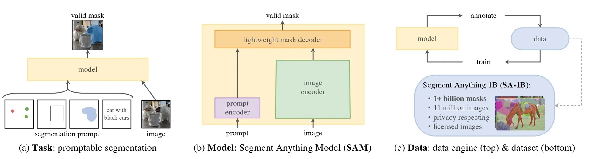
Core idea, task, and motivation SAM treats segmentation as answering a generic, prompt-conditioned query rather than predicting a fixed set of semantic classes. Given an image \(I\) and a prompt \(P\), the model outputs multiple candidate masks and associated quality scores, \begin {equation} f_\theta :\ \langle I,\,P\rangle \longmapsto \big (\{m^{(k)}\}_{k=1}^{K},\,\{\hat {s}_k\}_{k=1}^{K}\big ), \label {eq:chapter15_sam_prompt} \end {equation} where \(P\) may be a foreground/background point, an axis-aligned box, or a coarse mask; \(\{m^{(k)}\}\) are binary mask hypotheses; and \(\{\hat {s}_k\}\) are predicted IoUs used for ranking or automatic selection. In this formulation, prompts externalize the intent (which object in the scene?), while SAM specializes in delineation (where exactly is its boundary?).
This decoupling directly addresses the limitations of classical detectors and segmenters, which must jointly decide what and where from a fixed label set. In closed-set models, anything outside the training taxonomy is effectively “unknown”, and adding a new category requires collecting dense masks and retraining. In SAM, intent is supplied externally: detectors, text-grounding models, or simple heuristics propose regions (boxes or points), and SAM upgrades them to precise masks. By not baking a semantic label space into the segmentation module, SAM becomes a reusable, label-agnostic mask engine that composes with many upstream systems.
Three design pillars underpin this formulation:
- 1.
- Encode once, decode many. A large ViT encoder, pre-trained as a masked autoencoder, computes a dense image embedding once per image and caches it. Subsequent prompts reuse this embedding, so only a lightweight decoder is invoked per query, enabling millisecond-level interactive updates.
- 2.
- Promptable, open-set task. Prompts supply “which thing?” without class labels, allowing SAM to focus on a largely class-agnostic notion of segmentable objects: regions with closed boundaries, coherent parts, and consistent appearance. This makes the task naturally open-set and suitable for zero-shot transfer across many, though not all, domains.
- 3.
- Ambiguity awareness. A single prompt is often ambiguous (e.g., a click on a torso could mean shirt, person, or crowd). SAM therefore predicts several plausible masks \(\{m^{(k)}\}\) and scores them with \(\{\hat {s}_k\}\), so a user or system can select or refine the hypothesis that best matches intent instead of averaging incompatible solutions.
Architecture and SA-1B data engine These ideas are realized through a ViT-based architecture coupled with a self-bootstrapping data engine:
- Image and prompt encoders; mask decoder. A large ViT image encoder (e.g., ViT-H) produces a coarse but rich embedding \(E \in \mathbb {R}^{H/64 \times W/64 \times C}\) once per image and caches it. A prompt encoder converts points (2D coordinates with a foreground/background flag), boxes (corner coordinates), or downsampled masks into a small set of prompt tokens. A transformer-based mask decoder then fuses prompt tokens with \(E\) to produce \(K\) mask logits and their predicted IoU scores in tens of milliseconds on a modern GPU. During training, a min-over-masks objective matches only the best predicted mask in the set to the ground truth, encouraging the hypotheses to cover typical whole/part/subpart interpretations instead of collapsing to a single averaged mask.
-
SA-1B via a three-stage data engine. To support broad, open-set behavior, SAM is trained on SA-1B, a web-scale corpus of \(\sim \)1.1B masks over 11M licensed images. This dataset is constructed by an iterative data engine:
- 1.
- Assisted manual phase. Human annotators use early SAM variants as interactive tools to draw high-quality masks, seeding the dataset.
- 2.
- Semi-automatic phase. As SAM improves, it proposes masks given simple prompts (e.g., boxes), and annotators mainly verify or lightly correct them, dramatically increasing throughput.
- 3.
- Automatic phase. A strong SAM model runs in a “segment everything” mode: a grid of prompts across each image yields candidate masks that are filtered and deduplicated automatically, adding hundreds of millions of masks with minimal human effort.
The result is a diverse collection of masks for objects, stuff, and parts, providing the coverage needed to learn a broad, class-agnostic notion of objectness.
Zero-shot prompting, interaction, and ambiguity Because prompts supply intent, SAM can often generalize to new domains without fine-tuning [309]. Pretraining on SA-1B induces a class-agnostic sense of objectness (closed contours, part–whole structure, texture and contrast cues). At inference time, prompts are encoded as tokens that condition the decoder, which attends jointly to these tokens and the cached image embedding \(E\).
A typical interactive loop is:
- 1.
- Initial prompt. Start with a positive click near the interior of the target object or a loose box around it.
- 2.
- Select a hypothesis. Inspect the small set of returned masks; pick the one that best matches intent, often simply the highest-\(\hat {s}_k\) mask. A low maximum IoU signals that more guidance is needed.
- 3.
- Refine with sparse feedback. If the mask misses a region, add a positive click in the missing area; if it leaks into background or neighboring objects, add a negative click there. Re-running the decoder with updated prompts refines the mask while reusing the same image embedding.
- 4.
- Accept or reuse. Once satisfactory, the mask is accepted as the final output or reused as a dense prompt to further tighten boundaries.
In practice, prompts often induce a natural hierarchy of hypotheses: a whole object, a coherent part (e.g., clothing), and a finer subpart (e.g., a logo). The min-over-masks training encourages SAM to populate this hierarchy rather than settle on a single compromise mask.
Applications, limitations, and fine-tuning SAM’s promptable, ambiguity-aware design supports a wide range of workflows:
- Biomedical pathology. On high-resolution tiles (e.g., \(2048{\times }2048\) at \(20{\times }\)), a positive click inside a lesion yields whole/part/subpart masks (e.g., lesion core vs. lesion+halo). A few positive/negative clicks typically suffice to obtain high-quality lesion contours despite scanner and stain shifts.
- Remote sensing. A coarse box around a city block can be refined into masks that follow roof footprints rather than roads or vegetation; in “segment everything” mode, a grid of prompts plus IoU-based filtering and non-maximum suppression yields instance masks that can be polygonized for GIS layers.
- Creative photo/video editing. A click on hair produces masks at different granularity (entire person, hair-only). After selecting and lightly refining the hair-only mask, one can generate high-quality alpha mattes for recoloring or compositing.
- Robotics and 3D perception. Detectors provide coarse boxes; SAM upgrades them to precise instance masks, which are then used to compute silhouettes and principal axes for grasp planning, or to associate 2D regions with depth measurements in a 3D pipeline.
- Document layout and UI parsing. Positive clicks on text blocks or UI elements produce tight component masks that can be vectorized into regions for OCR, reading-order inference, or accessibility tools, avoiding brittle, hand-crafted heuristics.
Despite its strong zero-shot performance on many natural-image-like domains, SAM is not a magic solution for all settings. Its notion of objectness is learned from SA-1B, which is still biased toward web imagery.
In highly specialized or “weird” domains (e.g., certain medical modalities, industrial inspection, or non-optical sensors), zero-shot performance can be suboptimal, and practitioners routinely fine-tune SAM or adapt its lightweight components (e.g., via LoRA-style adapters or decoder fine-tuning) on a modest number of in-domain masks. In such cases, SAM should be viewed as a segmentation foundation model: it provides a strong, promptable starting point that substantially reduces annotation and training costs, but high-stakes applications may still require domain-specific adaptation and careful evaluation.
Summary. A unified prompt-conditioned interface \(\langle I,P\rangle \!\to \!\) masks, an encode-once/decode-many architecture for low-latency interaction, and a web-scale mask corpus together yield a segmentation foundation model that generalizes widely without task-specific retraining, serves as a fast interactive tool across domains, and can be further fine-tuned where necessary to meet stringent domain-specific requirements.
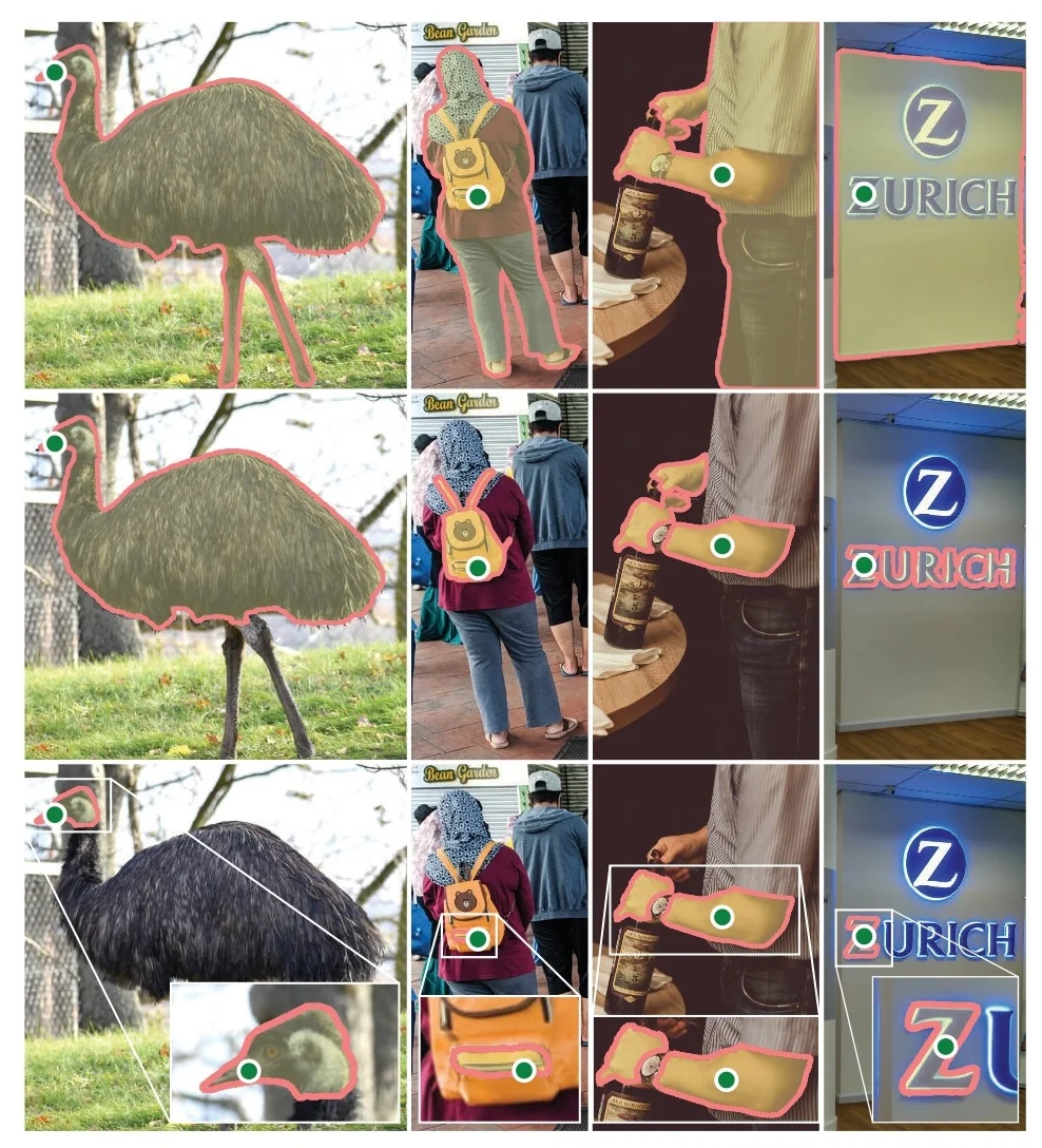
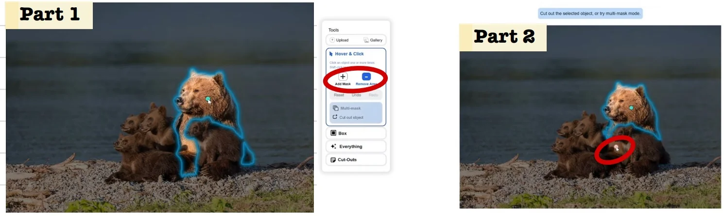
This interactive perspective sets up the detailed method next: SAM’s image encoder (a ViT pretrained via MAE [219]), prompt encoder (including point/box encodings and dense mask prompts), two-way mask decoder with cross-attention, and training losses (focal + dice with min-over-masks).
Method
Model overview and data flow SAM follows an encode once, prompt many design [309]. An input image (typically resized to \(1024{\times }1024\)) is passed once through a heavy image encoder to produce a cached dense embedding. At interaction time, a prompt encoder turns user intent (points, boxes, or a coarse mask) into compact tokens. A lightweight mask decoder then fuses prompt tokens with the cached image embedding via two-way attention and produces up to three candidate masks plus a predicted IoU score to rank them. In interactive use, the newly accepted mask is fed back as a dense prompt for the next refinement step, forming a fast loop: encode image \(\rightarrow \) decode mask(s) \(\rightarrow \) add corrective prompt(s) \(\rightarrow \) decode again, until satisfactory alignment.
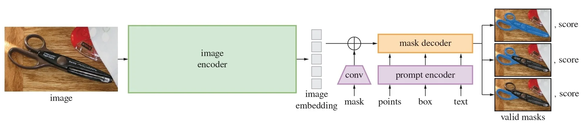
Image encoder The image encoder is a large Vision Transformer (ViT, e.g., ViT-H) initialized from MAE pretraining [219]. MAE masks a high fraction of image patches and learns to reconstruct them from the visible ones, yielding strong, general-purpose visual features. Given a \(1024{\times }1024\) input, the encoder produces a dense embedding on a lower-resolution grid (e.g., \(64{\times }64\) tokens) that SAM projects to a channel dimension \(C{=}256\) for efficient decoding [309]. This pass is amortized: it runs once per image and is reused for all subsequent prompts.
Prompt encoder SAM supports sparse and dense prompts in its official release; text enters only indirectly via external systems:
- Sparse prompts. Points are represented by their \((x,y)\) coordinates plus a learned type embedding indicating foreground, background, or padding; boxes are represented by their two corners (top-left, bottom-right), each with positional encodings summed with a corner-type embedding [309]. These yield \(d{=}256\)-dimensional tokens compatible with the image embedding.
- Dense prompts. A coarse mask (e.g., a previous prediction) is downsampled and linearly projected to \(d{=}256\), then added to the image embedding so that subsequent decoding is conditioned on the prior mask [309].
- On text prompts. The SAM paper defines prompts broadly and notes that, in principle, text embeddings (for example from CLIP [512]) could be injected as additional tokens into the prompt encoder. However, the publicly released SAM and SAM 2 models are trained and shipped with visual prompts only (points, boxes, masks) and have no built-in text encoder or phrase-level segmentation supervision [309, 529]. In practice, “text-prompted SAM” systems route text through a separate vision–language model (e.g., CLIP, Grounding DINO, OWLv2) to produce boxes or points, which are then fed to SAM/SAM 2 as standard sparse prompts. Native, end-to-end concept-level text prompting is introduced only later in SAM 3 (covered in a subsequent part).
Positional encodings for 2D prompts Goal and constraint. A prompt (point or box corner) is a continuous image coordinate \((x,y)\). Its embedding should satisfy two geometric desiderata: (i) locality: vectors for nearby points are similar and similarity decays with the Euclidean distance \(\|p-q\|_2\); (ii) isotropy: the decay is direction-agnostic (no axis bias), and the mapping extrapolates to arbitrary resolutions and subpixel locations.
Why standard PEs fall short. Absolute learned PEs in ViTs tie positions to a fixed grid index, hurting extrapolation to new resolutions. Separable 1D sinusoidal PEs [664] are continuous but anisotropic in 2D: concatenating \(\mathrm {PE}_x(x)\) and \(\mathrm {PE}_y(y)\) yields similarities that drop faster along axes than along diagonals at the same \(\|p-q\|_2\), biasing attention and making mask boundaries “slip” along \(x\)/\(y\).
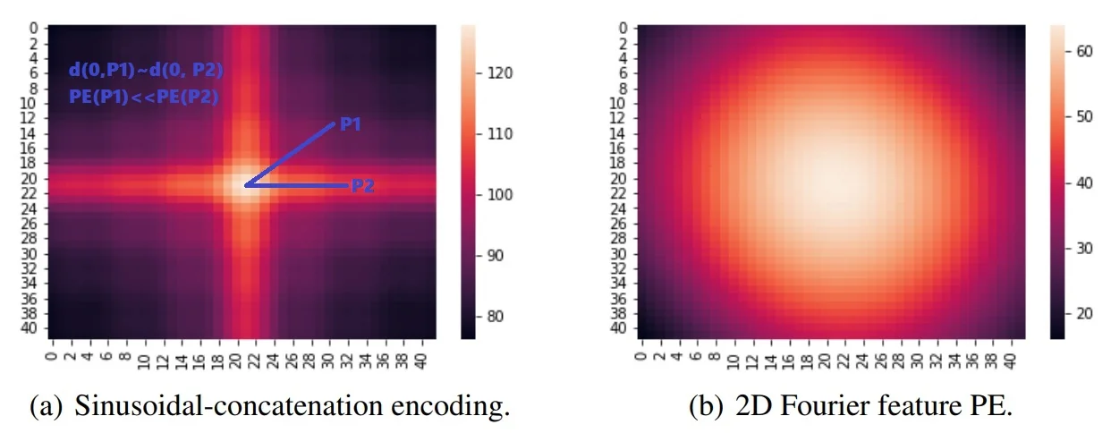
SAM’s choice: random Fourier features (RFF). SAM treats prompt coordinates as continuous and uses a joint 2D Fourier mapping [624]: \[ \gamma (x,y) \;=\; \begin {bmatrix} \cos \!\big (2\pi \,B\,[\hat {x},\hat {y}]^{\!\top }\big )\\[2pt] \sin \!\big (2\pi \,B\,[\hat {x},\hat {y}]^{\!\top }\big ) \end {bmatrix} \in \mathbb {R}^{2D},\qquad (\hat {x},\hat {y}) \in [-1,1]^2, \] where \(B\in \mathbb {R}^{D\times 2}\) has i.i.d. entries \(B_{ij}\sim \mathcal {N}(0,\sigma ^2)\) and \((\hat {x},\hat {y})\) are the normalized coordinates (e.g., \(\hat {x}=2(x/W)-1\), \(\hat {y}=2(y/H)-1\)). Each row of \(B\) defines a sinusoid over a tilted direction (a linear combination of \(x\) and \(y\)), so stacking rows yields a bank of multi-frequency, multi-orientation waves that respect 2D geometry. The final prompt token adds a small learned type embedding (e.g., foreground/background for points, corner identity for boxes): \(t=\gamma (x,y)+e_{\mbox{type}}\).
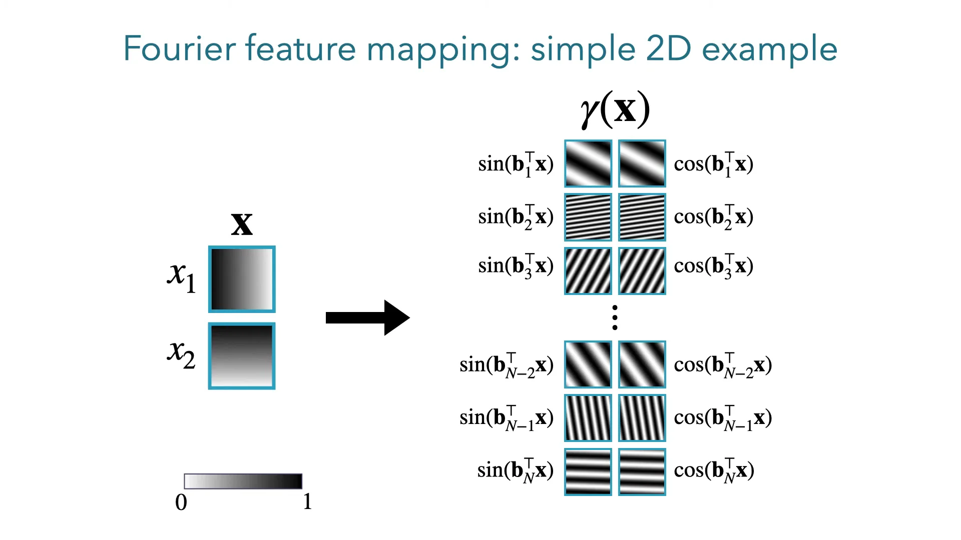
Why RFF helps—two lenses.
- Spectral-bias lens (representation). Coordinate-fed networks learn low frequencies first (“blurry” fits). Prepending \(\gamma (\cdot )\) injects high-frequency basis functions, letting shallow decoders express sharp edges with few updates [624]. Empirically, replacing raw \((x,y)\) or separable 1D PE with RFF improves fine boundary fidelity with fewer corrective clicks.
- Kernel/NTK lens (geometry). Wide networks trained by gradient descent behave like kernel machines with the Neural Tangent Kernel (NTK) [268]. With \(B\sim \mathcal {N}(0,\sigma ^2 I)\), the expected inner product of two encodings depends only on the offset \(\Delta =p-q\): \[ \mathbb {E}_{B}\!\left [\gamma (p)\!\cdot \!\gamma (q)\right ] \;=\; \exp \!\big (\!-\;2\pi ^2\sigma ^2\,\|\Delta \|_2^2\big ), \] i.e., a Gaussian RBF (up to constants). Thus, \(\sigma \) controls an isotropic notion of locality: small \(\sigma \) \(\Rightarrow \) wide kernel (smooth, risk of underfitting); large \(\sigma \) \(\Rightarrow \) narrow kernel (sharp, risk of aliasing). This aligns vector similarity with Euclidean distance—exactly what prompt geometry needs.
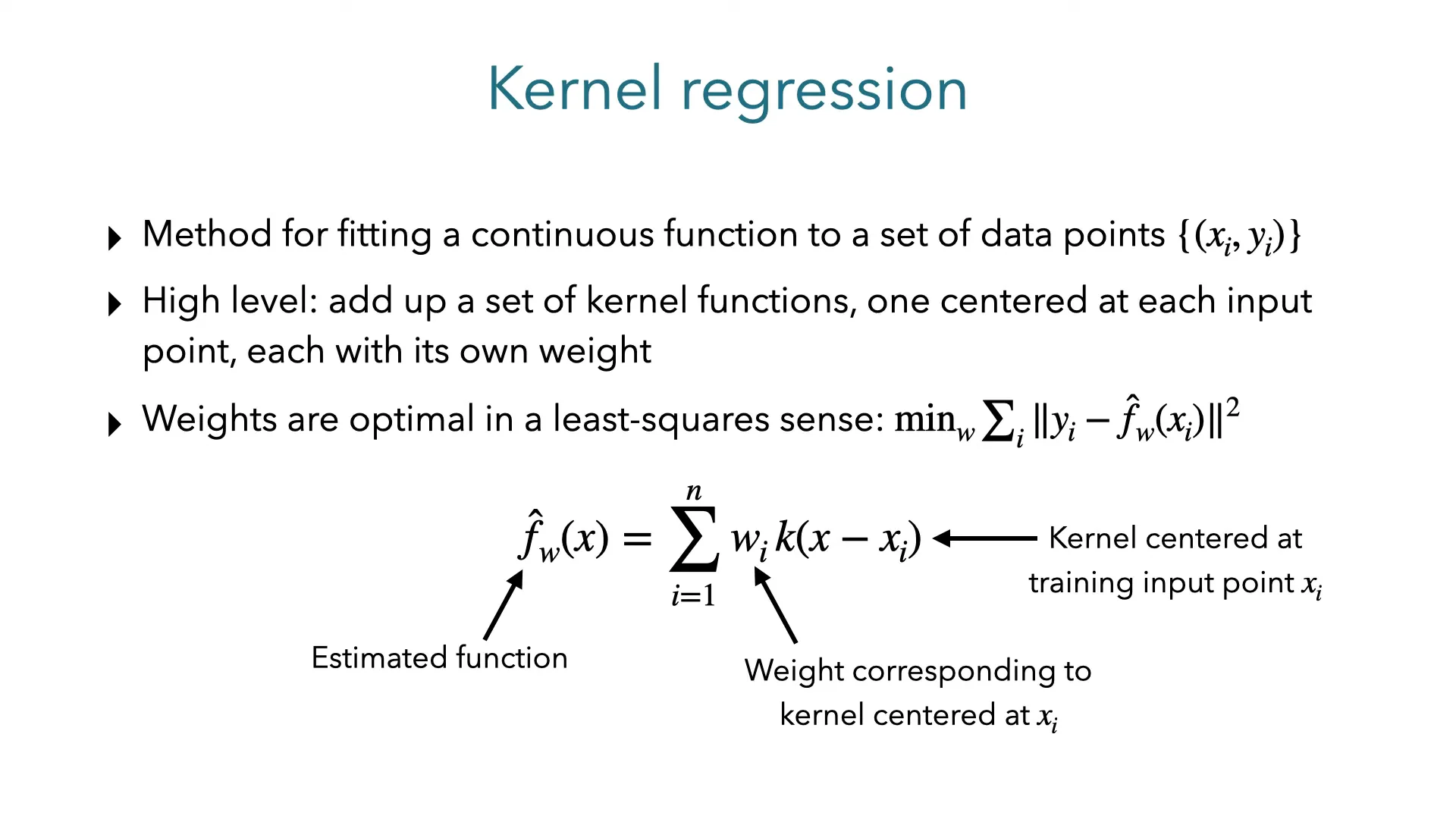
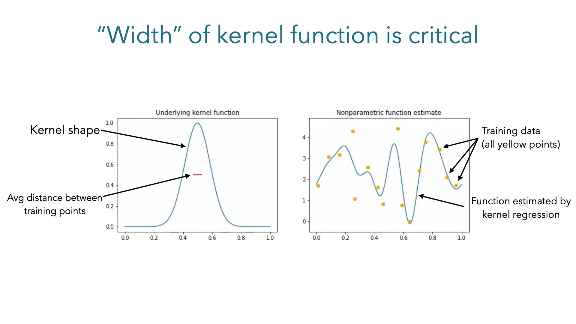
From derivation to practice. The RFF mapping arises from Bochner’s theorem: any shift-invariant positive-definite kernel has a nonnegative Fourier transform \(\hat {k}(\omega )\) with \(k(\Delta )=\mathbb {E}_{\omega \sim \hat {k}}[\cos (2\pi \,\omega ^\top \Delta )]\). Sampling \(\omega \) from a Gaussian \(\mathcal {N}(0,\sigma ^2 I)\) gives a Gaussian RBF kernel; Monte Carlo features \(\gamma (\cdot )\) approximate it [624]. Normalizing coordinates to \([-1,1]^2\) avoids phase wrapping and makes the code resolution-agnostic.
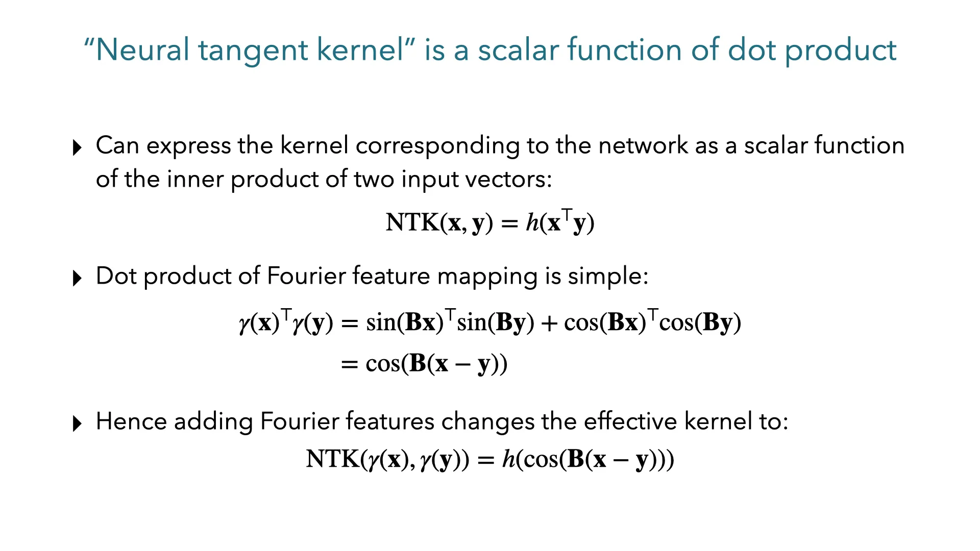
How to tune \(\sigma \) (and what SAM does). Choose \(\sigma \) by a small grid/linear search on validation data: fix a random \(B\) per \(\sigma \), evaluate a proxy (e.g., mIoU of point-to-mask or reconstruction PSNR in a coordinate MLP), and pick the best trade-off (sharp boundaries without aliasing). In SAM, \(B\) is sampled once and then frozen; \(\sigma \) is treated as a hyperparameter, keeping the prompt path parameter-free and fast at inference.
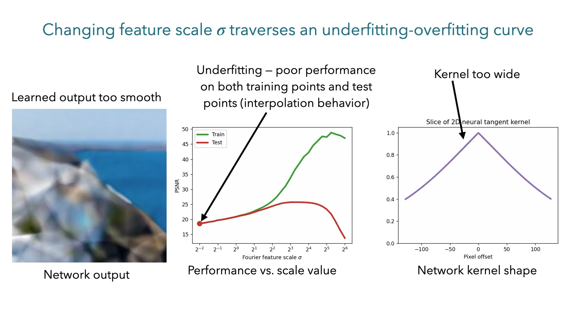
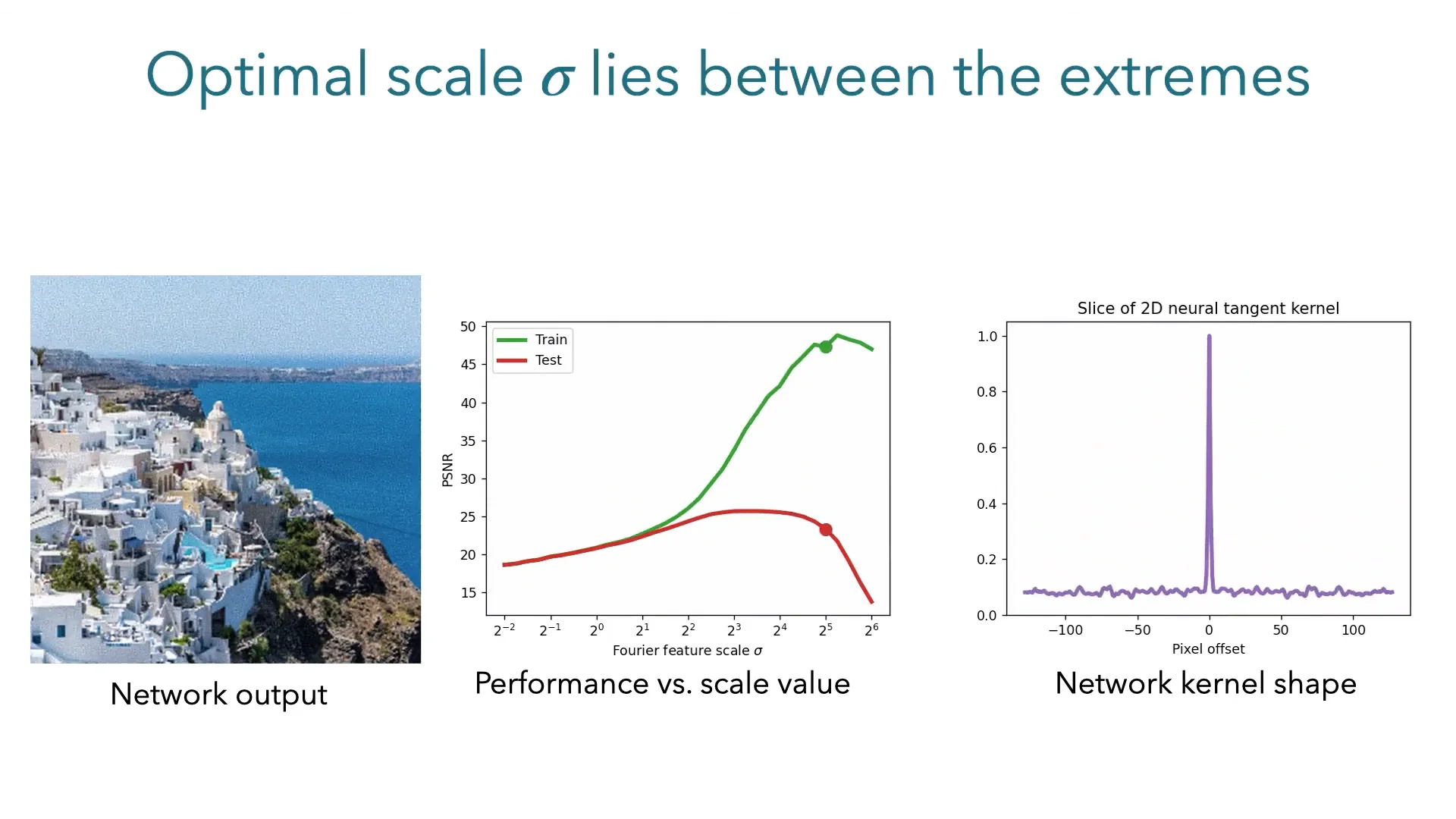
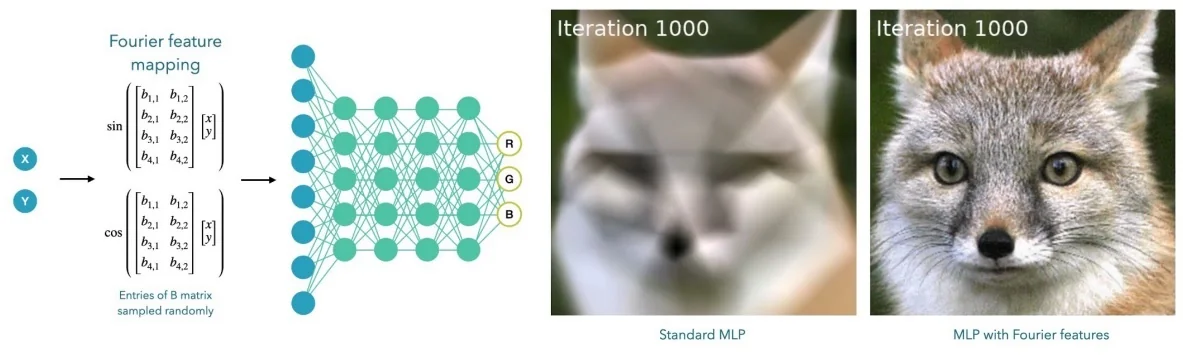
RFF Effect on SAM. Compared with separable 1D PE, RFF delivers:
- Isotropic locality. Similarity decays with \(\|p-q\|_2\), so point and box-corner tokens condition the decoder uniformly in all directions, reducing axis bias at boundaries.
- High-frequency readiness. The decoder’s small MLPs receive multi-frequency inputs, enabling crisp, click-efficient refinements around thin parts and textured edges.
Mask decoder (two-way attention and dynamic heads) High-level intuition. Once the heavyweight ViT encoder has produced a rich, cached feature map of the image, the mask decoder turns this static representation into an interactive tool. User prompts (points, boxes, and optionally a prior mask) are converted into a small set of prompt tokens that act as sparse “pins” indicating what the user cares about. The mask decoder, implemented as a lightweight two-layer transformer, runs a short two-way attention procedure: prompt tokens query the image embedding for visual evidence, and image features in turn query the prompts to understand which parts of the scene are relevant. This bidirectional exchange yields a set of prompt-aware features and updated tokens from which the decoder predicts a few candidate masks together with a quality score for each, enabling fast, interactive refinement.
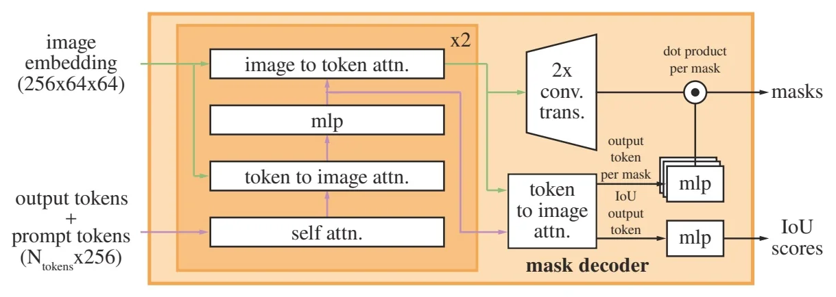
Two-way attention as a conversation. The two-way attention block can be viewed as a two-step “conversation” between prompts and image:
- Prompts \(\rightarrow \) image (token\(\rightarrow \)image attention). Prompt and output tokens ask the image embedding: “Where in this feature map is the evidence that supports my click or box?” Each token pulls in edges, textures, and contextual cues from relevant spatial locations.
- Image \(\rightarrow \) prompts (image\(\rightarrow \)token attention). Image features then ask back: “Given these prompts, which of them are relevant for this local patch?” This makes the image embedding prompt-aware, amplifying features consistent with the prompts and suppressing distractors (e.g., shadows or adjacent objects).
Because both directions are present, the prompts become evidence-aware and the image becomes intent-aware; neither side dominates, which is crucial for producing masks that both follow the user’s clicks and respect the global image structure.
Why this structure? Two-way attention avoids failure modes of one-sided designs: a prompt-only decoder might hallucinate shapes that match the clicks but ignore global context, while an image-only decoder might segment the most salient object and disregard the specific prompt. Learned mask tokens act as dynamic heads that specialize into different plausible extents (e.g., whole object, part, subpart) without introducing heavy per-pixel branches. A separate IoU token learns to predict the quality (approximate IoU) of each candidate mask, turning the set of hypotheses into a ranked list. In practice, this design yields high-quality, multi-mask predictions in tens of milliseconds, supporting real-time interaction [309].
Step-by-step (one decode).
- 1.
- Assemble inputs. Encode user prompts into tokens:
- Points are embedded from their image coordinates and a foreground/background flag.
- Boxes are embedded from corner coordinates.
- An optional coarse-mask token encodes a prior mask in sparse form.
If a previous mask was accepted, it is downsampled, projected, and added as a dense prompt to the image embedding. This biases features near the existing boundary, making interactive refinement more efficient in subsequent passes.
- 2.
- Add output tokens. Append four learned output tokens to the prompt
tokens:
- Three mask tokens, each responsible for producing one candidate mask.
- One IoU token, responsible for predicting the quality score of those masks.
These tokens start as content-agnostic vectors and will be shaped by the two-way attention blocks into object-specific descriptors.
- 3.
- Two-way block #1 (gather evidence). The first two-way attention
block runs three sub-steps:
- (a)
- Token self-attention. Prompt and output tokens attend to each other to fuse their cues. For example, multiple positive clicks on the same object reinforce one instance, while negative clicks help suppress distractors.
- (b)
- Token\(\rightarrow \)image attention. Tokens query the cached image embedding to retrieve spatial evidence, pulling in local structure (edges, textures) and part/whole context around the prompts.
- (c)
- Image\(\rightarrow \)token attention. Image features attend back to the current tokens, becoming prompt-aware by emphasizing regions that are compatible with the prompts. Positional encodings are added on the image side, and the original prompt embeddings (with position encodings) are re-added to token queries and keys to maintain stability and spatial anchoring [309].
After this block, tokens carry evidence-rich context and the image embedding is already shaped by user intent.
- 4.
- Two-way block #2 (synthesize and refine). A second, identical two-way block repeats the three sub-steps on the updated tokens and image features. The first block primarily gathers evidence; the second synthesizes it, refining object boundaries and resolving ambiguities such as part-versus-whole choices.
- 5.
- Predict masks and scores. Finally, the prompt-aware image embedding
is upsampled with lightweight transposed convolutions to a decoder
resolution (e.g., \(256 \times 256\)).
- Each mask token passes through a small MLP to produce a mask embedding. A dot product between this embedding and the upscaled feature map at each spatial location yields one logit map per mask token, corresponding to different hypotheses (e.g., whole object, part, subpart).
- The IoU token is fed through its own MLP to predict a scalar quality score for each mask, trained to approximate its IoU with the ground-truth mask.
The resulting masks are produced at decoder resolution and then resized to the original image resolution (or to the box region) for visualization and downstream use. The highest-scoring mask can be selected automatically, while alternative hypotheses are available for interactive correction.
Training objective and loss High-level goal (how to supervise a promptable model). Classical segmentation trains a network to label all pixels at once. SAM instead learns a conditional mapping \(\langle I,\mbox{prompt}\rangle \!\mapsto \! \mbox{mask(s)}\), so supervision must (i) treat points/boxes as inputs, not targets; (ii) compare only predicted masks to ground-truth; and (iii) support multiple hypotheses because a single prompt can mean whole/part/subpart. The losses below implement this recipe efficiently at SA-1B scale [309].
Targets and supervision signal. Each training example consists of an image \(I\) and a binary, pixel-accurate instance mask \(M \in \{0,1\}^{H\times W}\) for a single segment (foreground \(=1\), background \(=0\)). SAM is trained to predict a mask \(\hat {M}\) conditioned on a prompt \(P\); it does not predict boxes or points themselves. During training, prompts are simulated from \(M\) (see below). Supervision always compares \(\hat {M}\) against \(M\) (mask–vs–mask); there is no box loss.
Prompt simulation (teaching interactivity without human clicks). To expose the decoder to realistic inputs, we synthesize prompts \(P\) from \(M\):
- Positive / negative points. Sample positives uniformly inside \(M\); sample negatives outside \(M\) (optionally biased near the boundary to mimic corrective clicks).
- Boxes. Use the tight bounding rectangle of \(M\), then apply random scale/aspect jitter; optionally draw from cropped regions to vary context.
- Dense prior (previous mask). Downsample \(M\) (or a perturbed version via erode/dilate) to form a coarse “dense prompt” used for refinement training.
- Multi-round chains. In a subset of batches, decode once, place corrective points on disagreement regions, and decode again—simulating click–refine loops.
Prompts are inputs; supervision remains purely mask–vs–mask.
Multi-hypothesis supervision (min-over-masks). Given one prompt, the decoder emits up to three plausible masks \(\{\hat {M}_j\}_{j=1}^3\subset [0,1]^{H\times W}\) to capture whole/part/subpart ambiguity. With only one ground truth \(M\), we compute a segmentation loss for each \(\hat {M}_j\) and backpropagate through the best one: \[ \mathcal {L}_{\mbox{seg}} =\min _{j\in \{1,2,3\}} \Big [\, \lambda _{\mbox{focal}}\,\mathcal {L}_{\mbox{focal}}(\hat {M}_j,M) +\lambda _{\mbox{dice}}\,\mathcal {L}_{\mbox{dice}}(\hat {M}_j,M) \,\Big ]. \] Intuition: under an ambiguous prompt, we want at least one candidate to match the user’s intent. The “min” lets the three heads specialize (e.g., one tends to whole, one to part) instead of collapsing all to the same mask. A strong focal:dice ratio (reported \(20{:}1\)) emphasizes boundary decisions under severe fg/bg imbalance [309].
Loss components (what they measure and why).
- Focal loss combats extreme class imbalance by down-weighting easy pixels and amplifying hard ones near edges. With logits \(z\) and post-sigmoid probability \(p=\sigma (z)\), for a target \(y\!\in \!\{0,1\}\) the binary focal loss is \[ \mathcal {L}_{\mbox{focal}}(p,y) =-\alpha _t(1-p_t)^{\gamma }\log (p_t), \quad p_t=\begin {cases} p,&y=1\\ 1-p,&y=0 \end {cases} \] with typical \(\gamma \!>\!0\) and \(\alpha _t\) rebalancing fg/bg. In SAM, this term dominates to focus learning where it matters most (thin structures, uncertain boundaries).
- Dice loss directly optimizes region overlap (shape agreement). For probabilities \(\hat {M}\in [0,1]^{H\times W}\), \[ \mathcal {L}_{\mbox{dice}}(\hat {M},M) =1-\frac {2\,\langle \hat {M},M\rangle + \varepsilon }{\|\hat {M}\|_1+\|M\|_1+\varepsilon }, \] where \(\langle \cdot ,\cdot \rangle \) sums pixelwise products and \(\varepsilon \) stabilizes small masks. Dice penalizes false positives/negatives at the shape level, complementing focal’s pixel focus.
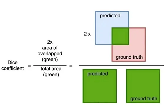
Quality calibration (IoU head). Beyond masks, SAM predicts for each hypothesis a scalar \(\hat {s}_j\) that should approximate the true IoU, \[ \mathrm {IoU}(\hat {M}_j,M)=\frac {|\hat {M}_j\cap M|}{|\hat {M}_j\cup M|}. \] A simple MSE trains this calibration: \[ \mathcal {L}_{\mbox{iou}}=\frac {1}{3}\sum _{j=1}^{3}\big (\hat {s}_j-\mathrm {IoU}(\hat {M}_j,M)\big )^2. \] At inference, \(\hat {s}_j\) ranks candidates and flags low-confidence cases (“add a click?”), matching SAM’s interactive use.
Total objective and gradients. The overall loss is \[ \mathcal {L} = \mathcal {L}_{\mbox{seg}} + \lambda _{\mbox{iou}}\mathcal {L}_{\mbox{iou}}, \quad \mbox{with }\lambda _{\mbox{iou}}=1 \mbox{ in~\cite {kirillov2023_sam}}. \] Let \(\ell _j=\lambda _{\mbox{focal}}\mathcal {L}_{\mbox{focal}}(\hat {M}_j,M)+\lambda _{\mbox{dice}}\mathcal {L}_{\mbox{dice}}(\hat {M}_j,M)\). If \(j^\star =\arg \min _j \ell _j\), then \(\nabla \mathcal {L}_{\mbox{seg}}=\nabla \ell _{j^\star }\) (other branches receive no seg-gradients), encouraging diversity across heads while the IoU head learns to score all candidates.
Why this works (design intuition).
- Prompt-conditioned supervision teaches the decoder to “follow the cue” rather than memorize taxonomies—key for zero-shot transfer.
- Min-over-masks aligns training with usage: present alternatives, let one match intent, keep others diverse for ambiguity.
- Focal+Dice balances boundary hardness and global overlap—crucial when fg pixels are scarce and shapes vary widely.
- IoU calibration closes the loop for interactivity: the model not only proposes masks but also knows which is best and when to ask for help.
Pseudo-code for interactive inference Single image, multi-round interaction.
- 1.
- Encode once: \(E \leftarrow \textsc{ImageEncoder}(I)\) (cache the heavy image embedding).
- 2.
- Repeat until accepted:
- (a)
- Encode prompt: \(P \leftarrow \textsc{PromptEncoder}(\mbox{points},\,\mbox{boxes},\,M_{\mbox{prev}})\), where \(M_{\mbox{prev}}\) is the previously accepted mask used as a dense prompt (optional).
- (b)
- Decode: \((\hat {M}_1,\hat {M}_2,\hat {M}_3,\hat {s}_1,\hat {s}_2,\hat {s}_3) \leftarrow \textsc{MaskDecoder}(E,P)\).
- (c)
- Select & display: \(j^\star = \arg \max _{j\in \{1,2,3\}} \hat {s}_j\); render \(\hat {M}_{j^\star }\) at image resolution.
- (d)
- Refine or stop: If boundaries deviate, add a positive point to include a missed region or a negative point to exclude leakage; set \(M_{\mbox{prev}} \leftarrow \hat {M}_{j^\star }\) and repeat. Otherwise, accept the mask.
Data engine and SA-1B
The authors construct SA-1B via a three-stage engine [309]: assisted manual collection (browser-based tool powered by early SAM), semi-automatic (detector-seeded prompts with human verification), and fully automatic generation using grid prompts and multi-scale crops followed by ranking, stability checks, de-duplication, hole-filling, and small-component pruning.
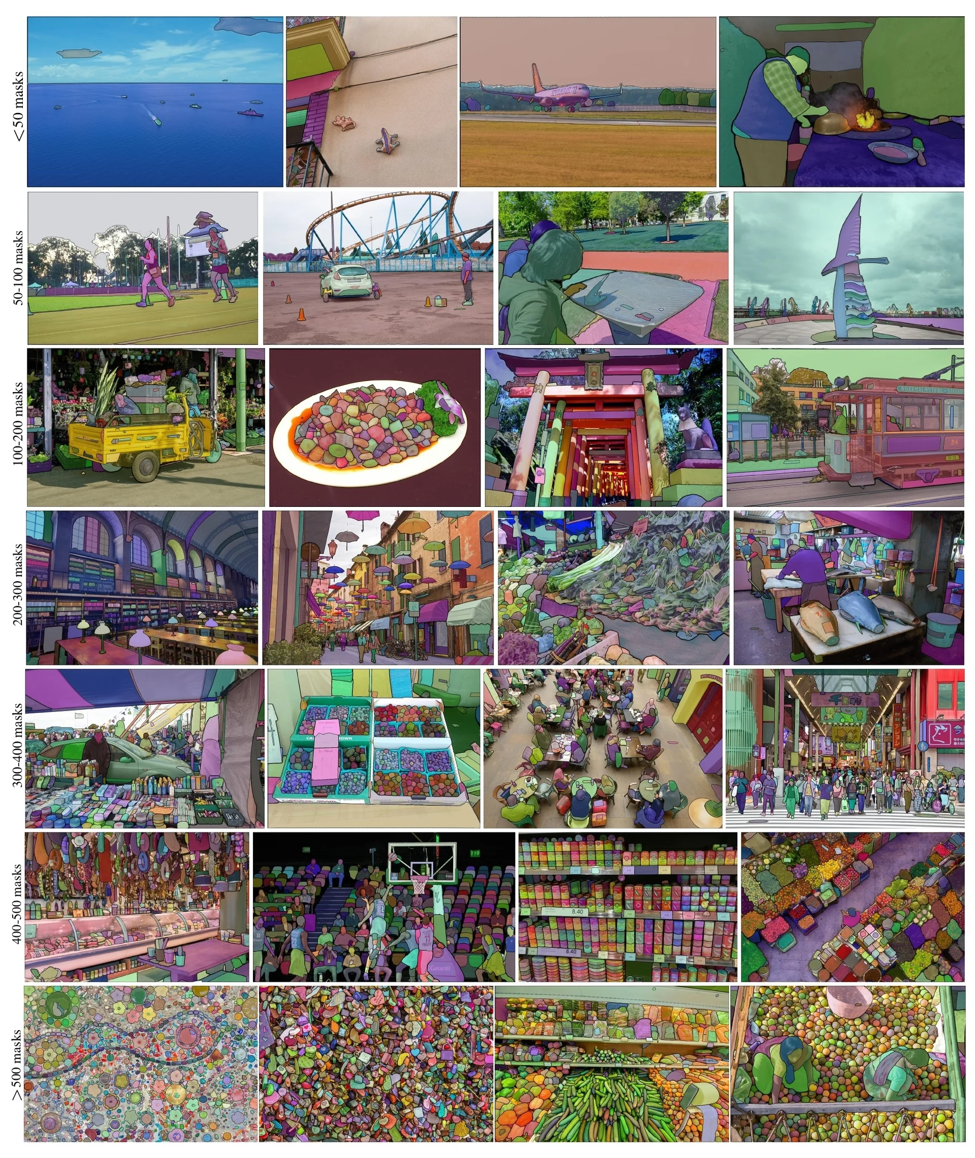
Dataset properties and diversity SA-1B is geographically and visually diverse, with broader coverage of object locations and shapes than prior datasets.
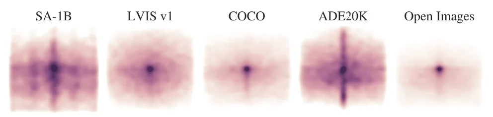
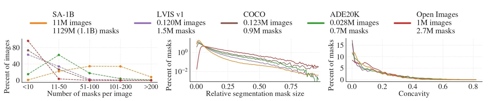
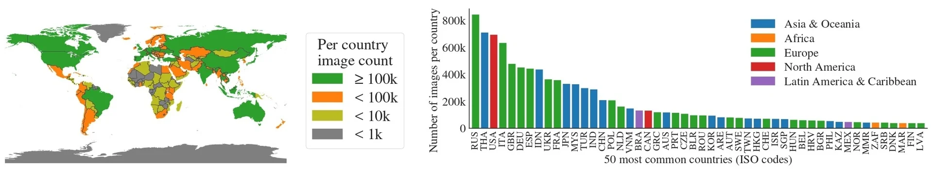
Experiments and ablations
Zero-shot samples across domains
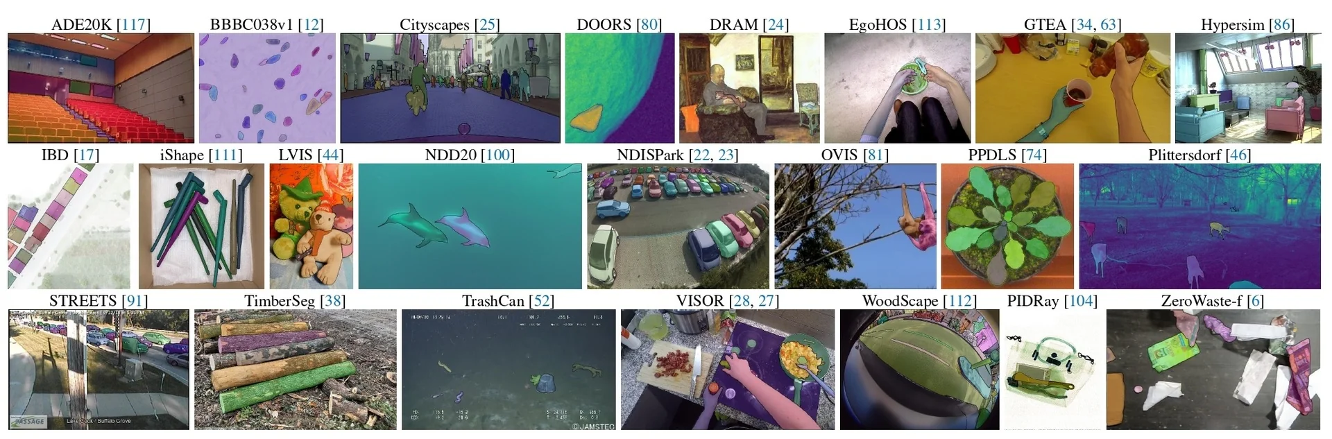
Interactive point-to-mask evaluation SAM is evaluated zero-shot on 23 unseen datasets with a simulated interactive protocol (place a point on the largest error, iterate) and both one-click and multi-click metrics [309]. On the one-click setting, SAM exceeds prior interactive baselines on 16/23 datasets and the gap reaches +47 mIoU on some sets; when an oracle picks the best of its three hypotheses (SAM–oracle), it outperforms all baselines on all 23 datasets [309]. Human quality ratings fall in the 7–9 range (Likert-style) and SAM’s oracle masks are rated close to ground truth, indicating high fidelity [309]. Multi-click curves show steady gains with diminishing returns after about ˜8 clicks; the training curriculum mirrors this with sequences up to 11 interactions to teach refinement [309].
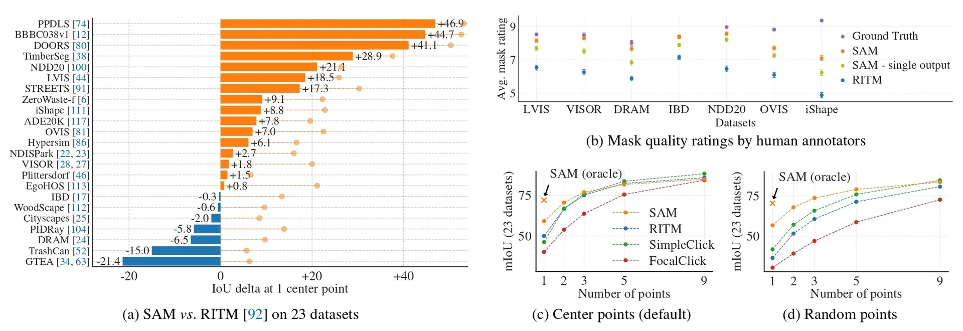
- Multi-mask hypotheses + min-over training. Predicting multiple masks per prompt and supervising with a min-over-masks loss lets the model represent whole/part/subpart alternatives without averaging incompatible solutions; it is a core ingredient in SAM’s ambiguity handling and one-click strength [309].
- Two-way attention in the decoder. Letting tokens query image features and image features query back the tokens (prompt-aware feature refinement) improves mask quality versus token\(\rightarrow \)image only; the authors report this bidirectional variant as particularly helpful for ambiguous, sparse prompts [309].
- Prompt encodings with Fourier features. Using random Fourier feature (RFF) positional encodings for sparse prompts yields near-isotropic geometry and better alignment than separable 1D encodings or raw coordinates, reducing axis-bias in point/box conditioning [309, 624].
- IoU prediction head for ranking. A small head trained to predict the mask IoU enables reliable automatic selection among the three hypotheses; in aggregate plots, SAM’s auto-selected mask tracks the oracle closely, validating the calibration [309].
- Interactive curriculum. The evaluation and training are aligned: simulated clicks are placed on the largest current error, improvement slows after ˜8 clicks, and SAM is trained with sequences up to 11 interactions to learn the refine–correct loop [309].
Limitations and future directions
- Heavy encoder cost. The ViT-H encoder is computationally expensive; although amortized for interactivity, deployment on resource-limited devices is challenging. Subsequent works (e.g., SAM 2) explore efficiency and streaming settings.
- Open-vocabulary text-to-mask. Fully integrated text grounding is limited in SAM; later systems combine grounding detectors (e.g., Grounding DINO) with SAM for text-to-region prompts, leading to Grounded-SAM variants.
- Fine structures and thin parts. Performance can degrade for extremely thin or low-contrast structures; higher-resolution backbones and tailored decoders are active directions.
- Temporal/video. SAM operates on single images; extensions to video streaming and memory-aware decoding are developed in SAM 2, covered next.
Enrichment 15.7.2: SAM 2: Segment Anything in Images and Videos
Context. We proceed to cover SAM 2 [529], the video-capable successor to SAM [309]. SAM 2 extends promptable segmentation from single images to videos by equipping a SAM-like encoder–decoder with a streaming memory that maintains object state over time. As before, we assume familiarity with encoder–decoder transformers and MAE-style pretraining; full treatments of Vision Transformers and self-supervised pretraining appear later in the book (as for SAM).
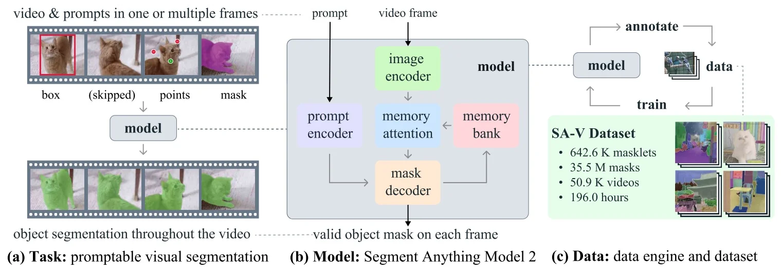
Core idea: streaming memory for video SAM 2’s central contribution is a streaming memory bank maintained per tracked instance. Instead of storing full frames, the system keeps compact tokens summarizing past accepted masks and prompts. This yields two complementary behaviors:
- Propagation. For each new frame \(t\), the decoder reads instance-specific memory tokens, fuses them with the current-frame features, and predicts the mask for that frame. Prior masks act as a strong prior for the object’s location and appearance, so the model effectively refines an existing estimate rather than re-segmenting from scratch.
- Recovery. When propagation drifts (e.g., due to occlusion or fast motion), a user provides a corrective prompt on some later frame \(t^\star \). The model produces a corrected mask, encodes it into new tokens, and writes them into memory. Subsequent frames read this updated state and continue with the corrected identity, without re-annotating intermediate frames.
Thus SAM 2 preserves SAM’s promptable interface while adding a lightweight mechanism for temporal consistency and interactive correction in videos.
Motivation
SAM showed that an “encode once, decode many” architecture with promptable, ambiguity-aware decoding yields strong zero-shot segmentation on images [309]. Extending this paradigm to videos introduces additional requirements:
- Identity persistence. The same object must be followed through motion, deformation, occlusion, disappearance, and reappearance.
- Sparse correction. Users should be able to repair drifts with a few clicks rather than repeatedly re-prompting from scratch.
- Interactive speed. Per-frame latency must remain low for real-time annotation and editing, even on long sequences.
A naïve SAM + tracker pipeline struggles on all three fronts: the tracker does not share SAM’s notion of objectness, corrections on a later frame do not automatically propagate forward, and failures often require full reinitialization. SAM 2 addresses these limitations by coupling the promptable decoder to a streaming memory that aggregates compact embeddings of past masks and prompts. Every new prompt or correction is written into this memory, and each subsequent frame reads the updated state, so improvements on frame \(t^\star \) immediately benefit frames \(t{>}t^\star \) without revisiting earlier predictions.
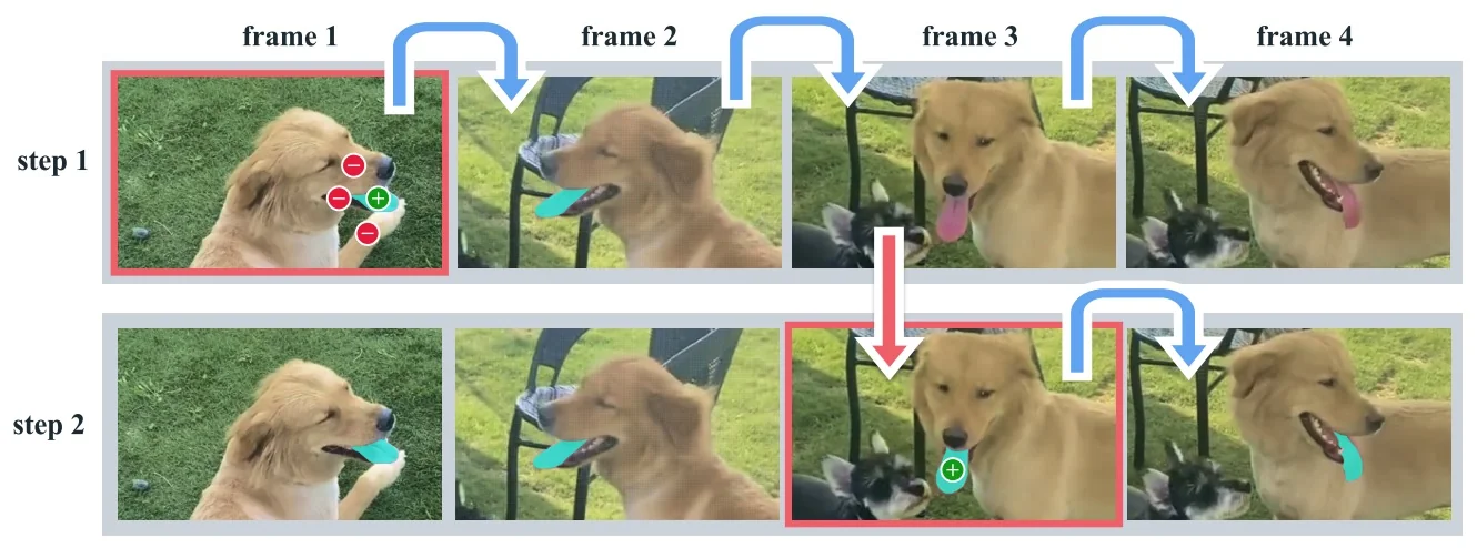
Method
Problem setup Given a video \(\{I_t\}_{t=1}^{T}\) and prompts \(\mathcal {P}\) provided on one or more frames (points, boxes, or masks), SAM 2 produces a temporally consistent mask \(\hat {M}_t\) per frame for the same instance specified by the prompts. A temporally contiguous run of such predictions for a single instance is called a masklet, i.e., a sequence of masks belonging to one object track. The system is designed to support:
- Image-only use (\(T{=}1\)), matching SAM.
- One-shot video prompting (prompts on an initial frame only, then fully automatic propagation).
- Sparse interactive corrections on arbitrary later frames, with each correction immediately influencing future predictions.
What is new compared to SAM SAM 2 preserves SAM’s basic decomposition (image encoder, prompt encoder, mask decoder) but augments it with temporal reasoning and a video-scale data engine:
- Streaming memory. For each tracked instance, SAM 2 maintains a dedicated memory bank of compact (\(\approx 64\)-dimensional) tokens distilled from past accepted masks and prompts. These tokens summarize both local appearance and coarse spatial position, and are much cheaper to store than full feature maps or frames. At each new frame, a bounded subset of tokens is retrieved (e.g., based on recency and/or similarity), providing identity cues at roughly constant per-frame cost.
- Memory-conditioned decoding. The lightweight decoder now conditions on three sources: current-frame image features, optional prompts on the current frame, and retrieved memory tokens. This injects temporal context directly into the promptable decoder without heavy re-encoding or explicit optical flow.
- Masklet supervision and video-scale data engine. Training uses SA-V, a large-scale video dataset with frame-wise masks grouped into masklets, disappearance/reappearance events, and model-in-the-loop propagation. Supervision is applied while the memory pathway is active, so the network learns to write informative tokens and to read them effectively for video segmentation.
To highlight the evolution from SAM to SAM 2, the following table summarizes key differences.
| Aspect | SAM [16] | SAM 2 [17] |
|---|---|---|
| Domain | Images. | Images + videos (promptable VOS). |
| Key new module | – | Streaming memory (per-instance). |
| Image encoder | ViT-H (MAE). | Hiera (hierarchical MAE) + FPN. |
| Training data | SA-1B (11M images). | SA-1B + SA-V (\(\sim 50\)K videos, \(\sim 642\)K masklets). |
| Supervision mode | Image masks only. | Clip-level masks with memory active. |
| Per-frame throughput | \(\sim \)tens of FPS for images. | Real-time video (optimized predictor \(\sim 130\) FPS per object). |
Why streaming memory? Design goals The streaming memory in SAM 2 is tailored to promptable video segmentation with three main goals:
-
Interactive recovery. A corrective click and its resulting mask are encoded into new memory tokens that replace outdated information about the object. Later frames then read from this updated state, so propagation resumes from the corrected configuration rather than from a stale track.
- Efficient propagation. The decoder reuses prior memory tokens as a prior over the object’s location and appearance, reducing the amount of per-frame reasoning required to maintain a coherent track. Reading a bounded set of compact tokens keeps computation per frame approximately constant.
- Identity stability. Memory is instance-specific and selective: only the chosen hypothesis (the accepted mask) is written for that instance. This reduces contamination from competing masks and helps maintain a stable identity through occlusions, appearance changes, and background clutter.
High-level data flow At a high level, SAM 2 processes each frame \(t\) through a lightweight streaming pipeline:
- 1.
- Image encoding \(\rightarrow \) The current frame \(I_t\) is passed once through the Hiera+FPN backbone to produce dense multi-scale features; a main stride-\(s\) feature map \(F_t\) is cached for use by memory and the decoder.
- 2.
- Memory read \(\rightarrow \) For each tracked instance, a bounded subset of memory tokens is selected from its bank (e.g., based on recency and/or similarity). These tokens summarize past masks and prompts and provide identity-specific context.
- 3.
- Prompt encoding (optional) \(\rightarrow \) Any new clicks, boxes, or masks on frame \(t\) are encoded as prompt tokens \(P_t\), as in SAM.
- 4.
- Decoding \(\rightarrow \) The mask decoder fuses the current-frame features \(F_t\), retrieved memory tokens, and prompt tokens to predict up to three candidate masks \(\{\hat {M}_{t,j}\}_{j=1}^3\) with associated IoU scores. One mask is selected as the active hypothesis for that instance.
- 5.
- Memory write \(\rightarrow \) The selected mask and any prompts are transformed by a memory encoder into new tokens, which are appended to the instance’s memory bank (evicting the oldest entries if needed).
Together, these steps implement a constant-cost loop: encode frame \(\to \) read memory \(\to \) (optional) encode prompt \(\to \) decode masks \(\to \) write memory, sustaining interactive throughput over long videos.
Streaming memory mechanics We now outline the memory internals at a slightly more formal level. Let \(F_t \in \mathbb {R}^{C \times H \times W}\) denote the main stride-\(s\) feature map for frame \(t\). For each tracked instance, SAM 2 maintains a bounded memory bank \[ \mathcal {B} = \Big \{(K^{(j)}, V^{(j)}, \pi ^{(j)})\Big \}_{j \in \mathcal {J}}, \qquad |\mathcal {J}| \leq N_{\mbox{recent}} + N_{\mbox{prompt}}, \] where \((K^{(j)},V^{(j)}) \in \mathbb {R}^{HW \times d_k} \times \mathbb {R}^{HW \times d_v}\) are spatial key/value tokens distilled from frame \(j\), and \(\pi ^{(j)} \in \mathbb {R}^{d_o}\) is a compact object pointer that carries instance identity. Recent non-prompted frames are stored in a FIFO queue, while frames where the user interacted (prompts) are stored in a smaller, longer-lived queue so that corrections remain influential.
- What is stored. Let \(\hat {M}_t \in \{0,1\}^{H \times W}\) be the chosen mask for an instance at frame \(t\). A memory encoder \(g_{\mbox{mem}}\) gates the backbone features by the mask and projects them to key/value channels: \[ \tilde {F}_t = F_t \odot \mbox{Down}(\hat {M}_t) \in \mathbb {R}^{C \times H \times W}, \qquad (K^{(t)}, V^{(t)}) = g_{\mbox{mem}}(\tilde {F}_t), \] where \(\odot \) is channel-wise multiplication and \(\mbox{Down}\) resamples \(\hat {M}_t\) to match the stride \(s\). In practice, \(g_{\mbox{mem}}\) is a small conv/MLP stack that compresses channels \(C \to d_k,d_v\) and flattens spatially to \(HW\) tokens. Each token thus summarizes appearance and position for a visible part of the object. The pointer \(\pi ^{(t)}\) is derived from the decoder’s mask token for that instance (or a learned split of it); if an occlusion head predicts invisibility, a learned “occluded” embedding is added to \(\pi ^{(t)}\) to mark that the object is temporarily not visible.
- How memory is read. Before decoding frame \(t\), keys and values from all entries in \(\mathcal {B}\) are concatenated: \[ K_{\mathcal {B}} = [K^{(j)}]_{j \in \mathcal {J}} \in \mathbb {R}^{(HW|\mathcal {J}|) \times d_k}, \quad V_{\mathcal {B}} = [V^{(j)}]_{j \in \mathcal {J}} \in \mathbb {R}^{(HW|\mathcal {J}|) \times d_v}. \] Queries are obtained by projecting the flattened current-frame features, \(Q_t = \phi (F_t) \in \mathbb {R}^{HW \times d_k}\). A memory-attention stack computes \[ \mbox{MemAttn}(F_t,\mathcal {B}) = \mbox{softmax}\!\Big (\tfrac {Q_t K_{\mathcal {B}}^\top }{\sqrt {d_k}} + \Psi _{\mbox{pos}}\Big )\, V_{\mathcal {B}}, \] where \(\Psi _{\mbox{pos}}\) encodes 2D spatial (and short-range temporal) relations, typically via rotary or relative positional encodings. The object pointers \(\{\pi ^{(j)}\}\) are broadcast and concatenated to each \((K^{(j)},V^{(j)})\) to bias attention toward tokens of the target instance. The result is a memory-conditioned feature map \(F'_t\) with the same shape as \(F_t\), which is then fed into the mask decoder. Keeping \(|\mathcal {J}|\) small (e.g., a few recent frames plus a few prompted ones) ensures predictable \(\mathcal {O}(HW \cdot |\mathcal {J}|)\) cost and stable attention.
- How memory is written. After decoding frame \(t\), the system selects one hypothesis per instance (typically the mask with highest predicted IoU) and then writes \((K^{(t)},V^{(t)},\pi ^{(t)})\) into \(\mathcal {B}\), evicting the oldest unprompted entry if the bank is full. Because these tokens are derived from the same \(F_t\) and \(\hat {M}_t\) used by the decoder, every user correction immediately produces a new, informative memory entry that future frames can read. For multi-object tracking, each object maintains its own memory bank, while the image encoder and backbone features are shared across instances.
In summary, SAM 2 augments SAM’s promptable segmentation with a carefully designed streaming memory that enables efficient propagation, interactive recovery, and stable identities across time, all while preserving the same user-facing interface (points, boxes, masks) that made SAM broadly usable on images.
Prompt encoder We preserve SAM’s prompt vocabulary but make shapes explicit. For sparse prompts, a 2D point \(p\!=\!(x,y)\) in pixel coordinates is normalized to \([-1,1]^2\), then mapped by random Fourier features \(\gamma (p)\!=\![\sin (2\pi Bp),\cos (2\pi Bp)]\in \mathbb {R}^{2m}\) with \(B\in \mathbb {R}^{m\times 2}\) sampled once [624]. The final point token is \[ e_{\mbox{pt}}(p,\tau )=W_{\mbox{pt}}\,[\gamma (p)\,\|\,e_{\mbox{type}}(\tau )]\in \mathbb {R}^{d_p}, \] where \(\tau \in \{\mbox{fg},\mbox{bg},\mbox{pad}\}\) and \(e_{\mbox{type}}\) is a learned embedding. Boxes are encoded by four corner points with distinct corner-type embeddings and optionally by \((x_c,y_c,w,h)\) as a second token. Dense prompts (masks) use a small conv projector \(h\) to produce \(D\!=\!C\)-channel features at stride \(s\), then add to \(F_t\): \[ F_t^{\mbox{prompt}} = F_t + h(\mbox{Down}(M^{\mbox{in}})), \] so the mask acts as a soft spatial prior aligned to the backbone’s feature space [309].
Mask decoder with memory conditioning Let \(F'_t\) be the memory-conditioned map and \(P_t\) the (optional) prompt tokens. The decoder is a compact transformer with two-way token\(\leftrightarrow \)image attention as in SAM, extended with memory conditioning through \(F'_t\):
- Token SA: output tokens (three mask tokens \(m_k\) and one IoU token \(u\)) and prompt tokens self-attend.
- Token\(\rightarrow \)image CA: token queries attend to \(F'_t\) (flattened) to gather spatial evidence (token-to-image).
- Image\(\rightarrow \)token CA: image queries (from \(F'_t\)) attend to token keys to inject prompt/object context (image-to-token).
High-resolution skips from early encoder stages are fused late to restore detail. As in SAM, we emit up to \(K\!=\!3\) mask logits \(\{\hat {Y}_{t}^{(k)}\}\in \mathbb {R}^{H_\mbox{img}\times W_\mbox{img}}\) (after upsampling by light deconvs) and per-mask IoU scores \(\{\hat {s}^{(k)}_t\}\). The mask token state serves as the object pointer \(\pi ^{(t)}\) for memory writing. An auxiliary occlusion head (MLP on a dedicated token or pooled decoder state) predicts visibility \(\hat {y}^{\mbox{occ}}_t\in [0,1]\) so invisible frames do not incur mask loss.
Training objective and supervision Following SAM, we supervise only the best hypothesis per frame (min-over-masks). Let \(k^\star =\arg \min _k \mathcal {L}_{\mbox{seg}}(\hat {Y}_{t}^{(k)},Y_t)\) with \(\mathcal {L}_{\mbox{seg}}=\lambda _{\mbox{foc}}\mathcal {L}_{\mbox{focal}}+\mathcal {L}_{\mbox{Dice}}\). The total loss is \[ \mathcal {L} = \underbrace {\mathcal {L}_{\mbox{seg}}(\hat {Y}_t^{(k^\star )},Y_t)}_{\mbox{only }k^\star } + \lambda _{\mbox{IoU}}\!\sum _{k=1}^{K}\!\bigl \lVert \hat {s}^{(k)}_t - \mbox{IoU}(\hat {Y}_t^{(k)},Y_t)\bigr \rVert _1 + \lambda _{\mbox{occ}}\;\mbox{CE}\!\left (\hat {y}^{\mbox{occ}}_t,\,y^{\mbox{occ}}_t\right ), \] skipping \(\mathcal {L}_{\mbox{seg}}\) if \(y^{\mbox{occ}}_t{=}1\). Prompts are simulated as in SAM: positive/negative clicks sampled inside/outside \(Y_t\), jittered boxes from mask bounds, and dense prompts from prior predictions [309]. Crucially, training uses short clips \((t_1{<}\cdots {<}t_L)\) where early frames write memory \((\hat {M}_{t_\ell }\!\to \!\mathcal {B})\) and later frames read it (\(F'_{t_{\ell +1}}\!\leftarrow \!\mathcal {B}\)), mirroring deployment. Random temporal reversal (with probability \(0.5\)) regularizes for bi-directional propagation. We also apply teacher forcing by occasionally writing ground-truth masks to memory to stabilize early training, and memory drop (randomly masking entries in \(\mathcal {B}\)) to reduce over-reliance on any single view. SA-V clips with disappearance/reappearance provide explicit supervision for gap-robust propagation [529].
Pseudo-code for streaming interactive inference
- 1.
- Initialize \(\mathsf {Mem} \leftarrow \emptyset \).
- 2.
- For \(t{=}1,\dots ,T\):
- (a)
- \(F_t \leftarrow \texttt{ImageEncoder}(I_t)\).
- (b)
- \(P_t \leftarrow \texttt{PromptEncoder}(\texttt{points/boxes/mask at }t)\) (optional).
- (c)
- \(R_t \leftarrow \texttt{Select}(\mathsf {Mem})\).
- (d)
- \((\{\hat {M}_{t,j}\}, \{\hat {s}_{t,j}\}) \leftarrow \texttt{MaskDecoder}(F_t, R_t, P_t)\).
- (e)
- \(j^\star \leftarrow \arg \max _j \hat {s}_{t,j}\), output \(\hat {M}_t \leftarrow \hat {M}_{t,j^\star }\).
- (f)
- \(\mathsf {Mem} \leftarrow \texttt{Update}\!\big (\mathsf {Mem}, \texttt{MemoryEncoder}(F_t, \hat {M}_t, P_t)\big )\).
Architecture & Implementation Details
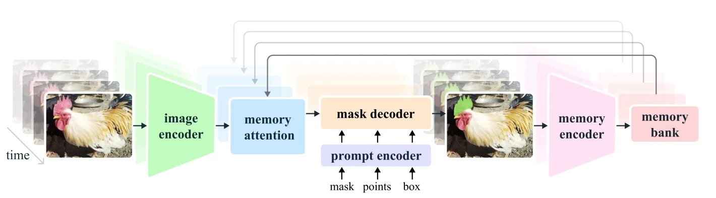
Backbone Large ViT-style encoders (e.g., Hiera variants) with MAE initialization produce a dense feature map per frame, reused within the frame.1
Prompt pathway Identical to SAM for sparse and dense prompts, with random Fourier features for 2D coordinate encoding (Section Enrichment 15.7.1).
Decoder A compact transformer augments SAM’s two-way attention with a memory cross-attention branch, outputting up to three masks and their IoU scores per frame.
Streaming memory Memory tokens are kept in a rolling buffer with constant-time selection (e.g., windowed or top-\(k\) retrieval) to preserve predictable per-frame cost. A memory encoder transforms the chosen prediction and frame features into new tokens.
Experiments and Ablations
SA-V dataset and data engine SAM 2 uses a model-in-the-loop engine extended to videos, producing SA-V with tens of millions of masks and hundreds of thousands of masklets. Qualitative examples appear in Figure 15.45 and dataset statistics in Table 15.4. The data engine phases demonstrate decreasing clicks and time per frame as SAM 2 is folded into the loop (see the below data-engine table).
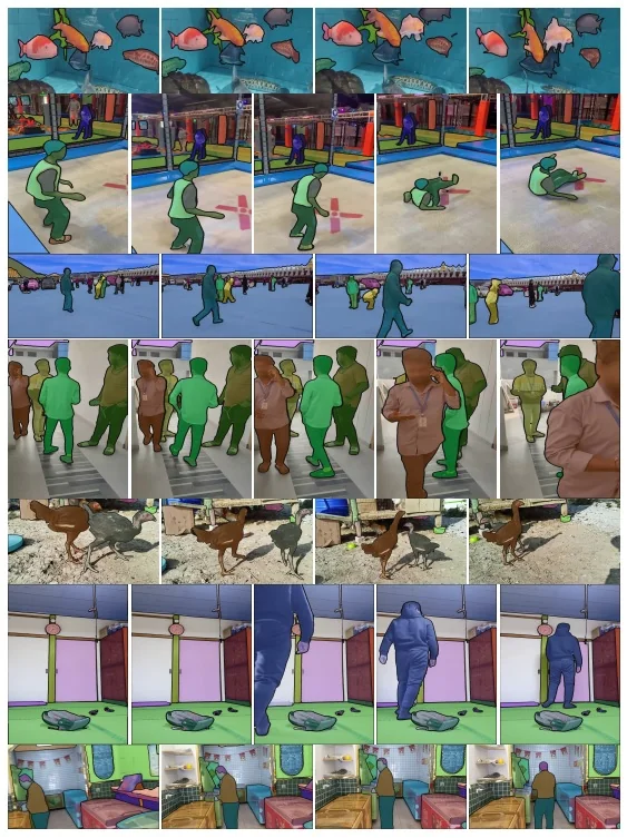
| Model in loop | Time/frame | Edited frames | Clicks/ | Phase 1 Mask Alignment (IoU>0.75) |
|||
|---|---|---|---|---|---|---|---|
| (s) | (%) | clicked frame | All | Small | Medium | Large | |
| Phase 1 SAM only | 37.8 | 100.00 | 4.80 | – | – | – | – |
| Phase 2 SAM + SAM 2 Mask | 7.4 | 23.25 | 3.61 | 86.4 | 71.3 | 80.4 | 97.9 |
| Phase 3 SAM 2 | 4.5 | 19.04 | 2.68 | 89.1 | 72.8 | 81.8 | 100.0 |
| Dataset | #Videos | Duration (hr) | #Masklets | #Masks | #Frames | Disapp. (%) |
|---|---|---|---|---|---|---|
| DAVIS 2017 | 0.2K | 0.1 | 0.4K | 27.1K | 10.7K | 16.1 |
| YouTube-VOS | 4.5K | 5.6 | 8.6K | 197.3K | 123.3K | 13.0 |
| UVO-dense | 1.0K | 0.9 | 10.2K | 667.1K | 68.3K | 9.2 |
| VOST | 0.7K | 4.2 | 1.5K | 175.0K | 75.5K | 41.7 |
| BURST | 2.9K | 28.9 | 16.1K | 600.2K | 195.7K | 37.7 |
| MOSE | 2.1K | 7.4 | 5.2K | 431.7K | 638.8K | 41.5 |
| Internal | 62.9K | 281.8 | 69.6K | 5.4M | 6.0M | 36.4 |
| SA-V Manual | 50.9K | 196.0 | 190.9K | 10.0M | 4.2M | 42.5 |
| SA-V Manual+Auto | 50.9K | 196.0 | 642.6K | 35.5M | 4.2M | 27.7 |
Zero-shot semi-supervised VOS SAM 2 outperforms decoupled SAM \(+\) tracker baselines across \(17\) video datasets under various prompt types (see the below table). The gain is largest for low-click regimes, reflecting the value of memory for propagation.
| Method | 1-click | 3-click | 5-click | Box | GT mask |
|---|---|---|---|---|---|
| SAM + XMem++ | 56.9 | 68.4 | 70.6 | 67.6 | 72.7 |
| SAM + Cutie | 56.7 | 70.1 | 72.2 | 69.4 | 74.1 |
| SAM 2 | 64.7 | 75.3 | 77.6 | 74.4 | 79.3 |
Segment Anything across 37 datasets Table 15.6 summarizes average 1- and 5-click mIoU on SA-23 (image) and \(14\) additional zero-shot video datasets, along with throughput.
| Model | Data | SA-23 All | SA-23 Image | SA-23 Video | 14 New Video / FPS |
|---|---|---|---|---|---|
| SAM | SA-1B | 58.1 (81.3) | 60.8 (82.1) | 54.5 (80.3) | 59.1 (83.4) / 21.7 |
| SAM 2 | SA-1B | 58.9 (81.7) | 60.8 (82.1) | 56.4 (81.2) | 56.6 (83.7) / 130.1 |
| SAM 2 | Our mix | 61.9 (83.5) | 63.3 (83.8) | 60.1 (83.2) | 69.6 (85.8) / 130.1 |
Ablations We summarize the most decision-shaping empirical findings the authors report across the main paper and appendices, focusing on the pieces that guided design choices (metrics follow VOS convention: region/boundary mean \(\mbox{J\&F }\); for images we use mIoU on the SA benchmarks).
Data mixture vs. architecture. Training only on images (SA-1B) already yields higher image mIoU for SAM 2 than SAM at substantially higher speed (e.g., with the Hiera-B+ image encoder: 58.9/81.7 1-/5-click mIoU vs. SAM ViT-H 58.1/81.3, while running \(\sim 6\times \) faster) and improves further when mixing videos (SA-V + internal + open VOS) to 61.4/83.7 and large gains on frames from video datasets (e.g., “14 new Video” average rises from 56.6/83.7 to 69.6/86.0). These tables isolate the data contribution versus pure architecture, establishing that joint image+video training is key for transfer to video frames while retaining strong image performance.
Speed/accuracy operating points. For semi-supervised VOS, the authors report real-time throughput with two encoder scales: Hiera-B+ at 43.8 FPS and Hiera-L at 30.2 FPS on a single A100 (batch size 1). The larger encoder improves accuracy across DAVIS/YTVOS/LVOS/SA-V, quantifying the classic capacity–speed trade-off and showing the decoder/memory remain light enough for interactive use.
Streaming memory design choices. Appendix C details the memory pathway used during ablations:
- Compact projections. Memory features are projected to 64-D, and the 256-D mask token (object pointer) is split into four 64-D tokens for cross-attention.
- Position encoding. Memory attention employs 2D RoPE for spatial (and short-range temporal) structure but excludes the pointer (no fixed spatial locus).
- Encoder reuse. The memory encoder reuses the image encoder’s embeddings instead of a second backbone.
These choices keep retrieval cheap and stable while improving long-horizon consistency. Although per-choice deltas are not tabulated as separate lines, these are the components retained in the final model after iterative experimentation.
Interactive robustness after failure cases. In the online/interactive protocol, SAM 2’s ability to prompt at any frame plus its streaming memory lets a single corrective click re-acquire objects after occlusion, unlike decoupled “SAM + tracker” pipelines that require re-annotation of full objects when drift occurs. Figure-level analyses (e.g., Fig. 2) explicitly compare the number and placement of clicks needed to recover, supporting the claim that memory is the dominant factor for robustness under occlusions/long motions in the interactive setting.
Dataset scale and coverage. The SA-V data engine (50.9K videos, \(\sim \)642.6K masklets) is shown to be much larger and more diverse (disappearance rates, geography, parts vs. wholes) than prior VOS datasets—motivating why memory-based propagation is learnable at scale and why performance saturates for prior methods on SA-V while SAM 2 keeps improving.
Takeaway. The evidence pattern is consistent:
- Joint image+video training establishes the base.
- The streaming memory pathway (with compact 64-D memories + object pointers + RoPE) translates that base into temporal robustness for occlusions/long motions.
- The decoder remains compact enough to preserve real-time throughput even at 1024-px inputs.
Limitations and Future Directions
We restate the authors’ limitations in spirit and connect each to concrete directions the community has begun to pursue. For deeper treatments, see SAMuRAI [745] (motion + memory selection for tracking), Grounded-SAM [540] and its video-centric follow-up Grounded-SAM 2 [263] (language-grounded detection/segmentation/tracking), and long-horizon memory variants such as SAM2Long [127].
- Memory selection at long horizons. The model “may fail to segment objects across shot changes and can lose track of or confuse objects in crowded scenes, after long occlusions or in extended videos”. This reflects a bounded, recency-biased FIFO memory that can evict rare but diagnostic past views. Next steps: learned retention/retrieval policies and compact identity-aware state (e.g., evolving object vectors); explicit shot-change handling. See also SAM2Long [127], which explores training-free tree memories to keep multiple hypotheses over long videos.
- Extreme appearance changes and fast motion. Severe deformations, lighting shifts, or thin/fast structures can induce drift before correction. Next steps: stronger temporal priors (optical flow cues; longer-range video transformers) and motion-aware selection. SAMuRAI [745] adds motion modeling and a motion-aware memory selection mechanism on top of SAM 2 for zero-shot tracking, improving robustness without fine-tuning.
- Dense multi-object interactions. Although SAM 2 can track multiple objects, independent per-object decoding can suffer identity swaps under heavy overlap or look-alike instances. Next steps: joint, conflict-aware reasoning (e.g., shared object-level context/graph layers) and stronger identity cues. Language-grounded pipelines such as Grounded-SAM and Grounded-SAM 2 [540, 263] help disambiguate identities with text-conditioned detection before segmentation/tracking.
- Prompt dependence and ambiguity. Ambiguous clicks can bias hypotheses; predicted IoU is a useful uncertainty signal but not a remedy. Next steps: UI policies that surface low-IoU regions and actively guide users to high-value clicks; integration with open-vocabulary grounding to replace ambiguous geometric prompts with unambiguous text prompts (cf. Grounded-SAM [540]).
- Domain coverage. Despite SA-V’s scale, niche modalities (thermal, medical, satellite) remain underrepresented. Next steps: continued data-engine iteration with targeted mining/verification and domain-specific adapters; language-grounded retrieval (as in Grounded-SAM families) can further lower annotation cost when scaling to new domains.
Implementation note. The official repository provides image/video predictors, checkpoints, notebooks, and an optimized video predictor with compiled kernels suitable for high-throughput VOS. The docs and Colab demonstrate interactive prompting, memory behavior, and speed/accuracy trade-offs out-of-the-box.
Enrichment 15.7.3: Mask DINO: Unified DETR-Style Detection and Segmentation
Motivation and Context
Mask DINO [340] is driven by a natural but ambitious question: Can one build a single DETR-style Transformer that, under one architecture and one training recipe, is competitive with state-of-the-art detectors on COCO while also achieving state-of-the-art performance on the major segmentation tasks (instance, panoptic, semantic) on benchmarks such as COCO and ADE20K? Before Mask DINO, the strongest models in these regimes were largely specialized: DINO-DETR [337] (built on DAB-DETR [382] and DN-DETR [338]) on the detection side, and Mask2Former [100] on the segmentation side. These models already share many ingredients (CNN or ViT backbones, multi-scale feature pyramids, Transformer encoders/decoders), but are each carefully tuned for their own objective and loss structure.
A natural baseline is to add a segmentation head on top of DETR or DINO-DETR and either fine-tune a detection-pretrained model or train the whole system from scratch in a multi-task fashion. In practice, both variants tend to be unsatisfactory.
Fine-tuning a detector with an added mask head Suppose we start from a DINO-DETR model pretrained for detection. Its decoder queries \[ Q = \{q_i\}_{i=1}^{N_q}, \qquad q_i \in \mathbb {R}^d, \] have been optimized to support classification and box regression, i.e., to predict \((c_i, \mathbf {b}_i)\) where \(\mathbf {b}_i \in \mathbb {R}^4\) is a coarse bounding box. Box losses encourage features that are good at capturing object extent and location, but do not explicitly enforce fine-grained, boundary-sensitive information. If we now attach a new mask head and fine-tune with an additional dense loss on masks \(\mathbf {m}_i \in [0,1]^{H \times W}\), two problems arise:
- At the beginning of fine-tuning, the new mask head sees queries \(q_i\) that are already specialized for boxes, not for detailed shapes. Early mask predictions are therefore poor, and the gradients from the mask loss attempt to substantially reshape \(q_i\), in conflict with the existing detection objective.
- Even after long fine-tuning, the model typically converges to a compromise where queries remain mostly box-oriented and the mask head learns to produce only approximate object silhouettes. The masks can improve over time, but they tend to lag behind strong segmentation baselines because the upstream query semantics were never designed with fine pixel-level accuracy as a primary goal.
In short, simply “bolting on” a mask head after detection pretraining gives the mask branch too little influence over how queries are formed and used throughout the network.
Training a unified detector+segmenter from scratch Alternatively, one can train DETR or DINO-DETR from scratch with both detection and segmentation losses active from the beginning. Here, the queries \(q_i\) are simultaneously pulled by a sparse, low-dimensional box loss (e.g., L1 and GIoU on \(\mathbf {b}_i\)) and a dense, high-dimensional mask loss (e.g., BCE or focal loss on \(\mathbf {m}_i\)). Without architectural mechanisms that explicitly couple how queries access spatial information, this often leads to:
- Noisy early supervision: Hungarian matching is typically dominated by box and class terms, so early in training the queries are encouraged to specialize for box-level localization first. Masks are then supervised on queries whose spatial alignment is still unstable, making mask gradients noisy and hard to use effectively.
- Gradient conflict: Box regression pushes queries toward features that summarize overall object geometry, while mask prediction pushes toward features that resolve local boundaries and textures. In a naïve multi-head setup these signals are not coordinated, so the model can settle at a compromise where neither detection nor segmentation reaches the level of specialized methods.
Running two separate models (a detector and a segmenter) avoids some of these issues but is computationally expensive and still fails to exploit potential synergies: detection predictions are not explicitly used to guide masks, and masks do not feed back to improve box localization or query selection.
Mask DINO: aligning detection and segmentation at the query level Mask DINO addresses these issues by taking DINO-DETR as its detection backbone and adding a tightly integrated segmentation branch instead of an independent head. Concretely, it brings in the Mask2Former idea of predicting masks via dot-products between query embeddings and a high-resolution pixel embedding map, while keeping DINO-DETR’s detection-oriented machinery (dynamic anchor boxes, mixed query selection, contrastive denoising, multi-scale deformable attention) largely intact. The core design principle is to align detection and segmentation at the level of queries and features, so that both tasks are driven by the same semantics and trained jointly from the earliest layers onward.
Formally, let \[ Q = \{q_i\}_{i=1}^{N_q}, \qquad q_i \in \mathbb {R}^d, \] denote the set of decoder content queries produced and refined by DINO-DETR (with \(N_q\) queries and hidden dimension \(d\)). Let \[ E \in \mathbb {R}^{H_4 \times W_4 \times d} \] denote a stride-4 pixel embedding map constructed from backbone and encoder features (the precise construction of \(E\) will be described later). Mask DINO makes the key decision to reuse these refined content queries as mask queries: the same token \(q_i\) that predicts an object’s category \(c_i\) and bounding box \(\mathbf {b}_i\) is also responsible for its mask \(\mathbf {m}_i\).
A lightweight mask head turns \(q_i\) into a mask embedding, and mask logits at stride 4 are obtained by per-location inner products \[ \ell _i(x,y) = \langle q_i, E(x,y) \rangle , \] followed by upsampling and a sigmoid to yield a full-resolution mask \(\mathbf {m}_i\). In parallel, the same \(q_i\) is fed to a classification head to produce \(c_i\) and to a box head to produce \(\mathbf {b}_i\).
Operationally, this yields a conceptually simple unified architecture in which a single set of queries feeds three heads in parallel—a class head, a box head, and a mask head—so that \((c_i,\mathbf {b}_i,\mathbf {m}_i)\) are all anchored to the same underlying query semantics and benefit from shared supervision. Detection-oriented components such as dynamic anchors, query denoising, and multi-scale deformable attention improve the quality and localization of queries, which in turn sharpens masks; conversely, dense mask losses help refine query semantics, which can improve classification and box regression. The remainder of this section explains how Mask DINO inherits and adapts components from DAB-DETR and DINO-DETR on the detection side, and from Mask2Former on the segmentation side, to realize this unified design and to substantially strengthen naïve “add-a-head” baselines.
From DAB-DETR and DINO-DETR to Mask DINO
Dynamic anchor boxes in DAB-DETR Vanilla DETR represents each decoder query as a learned content embedding plus a fixed sinusoidal positional encoding. In this design, a single vector must implicitly discover both what object it represents and where that object is likely to be, purely through end-to-end training. Queries therefore start “geometry-agnostic”: early in training they attend rather uniformly over the feature map, and the model only gradually learns to concentrate attention near object extents. This makes localization hard to optimize, slows convergence, and makes performance sensitive to initialization and training schedule.
DAB-DETR [382] makes this positional component explicit and refinable by turning it into a 4D anchor box that is updated at every decoder layer. Concretely, each query \(i\) at decoder layer \(\ell \) is represented as a pair \[ q_i^{(\ell )} \in \mathbb {R}^d, \qquad a_i^{(\ell )} = \bigl (c_x^{(\ell )}, c_y^{(\ell )}, w^{(\ell )}, h^{(\ell )}\bigr ) \in [0,1]^4, \] where \(q_i^{(\ell )}\) is a content embedding encoding “what” the query looks for (appearance and semantics), and \(a_i^{(\ell )}\) is a normalized box encoding “where” this query currently believes its object lies (box center and size, relative to the image).
At each decoder layer, a shallow MLP predicts an offset to the previous anchor, \[ \Delta a_i^{(\ell )} = f_{\mbox{box}}\!\bigl (q_i^{(\ell -1)}\bigr ), \qquad a_i^{(\ell )} = a_i^{(\ell -1)} + \Delta a_i^{(\ell )}, \] so boxes are refined coarse-to-fine across layers rather than being regressed in a single step from a fixed prior. This iterative refinement has two important consequences:
- Each layer only needs to predict a small correction to an existing box hypothesis, which is an easier optimization problem and leads to smoother gradients than one-shot regression from scratch.
- Early layers can focus on rapidly moving anchors from generic priors toward roughly correct regions, while later layers spend their capacity on tightening boxes around object boundaries.
In practice this significantly accelerates training and improves detection quality compared to vanilla and Conditional DETR.
The updated anchor \(a_i^{(\ell )}\) is then converted into a positional embedding (via a sinusoidal mapping) and added to the content query \(q_i^{(\ell )}\) before cross-attention, so that each query carries both semantic and geometric information. In the DAB-DETR implementation built on Deformable DETR, these anchors play a second, crucial role: their centers are used as reference points for multi-scale deformable attention. Rather than attending over all spatial locations in each feature map, each query samples only a small set of offsets around its current anchor, across multiple FPN levels. For a given query, attention thus operates on a fixed budget of \(M\) sampling points per head and per scale, whose positions are predicted relative to the anchor center. Larger, less precise anchors induce broader sampling patterns; as anchors are refined, the sampling region narrows around the object.
This “anchor-as-reference” mechanism is both statistically and computationally attractive:
- Statistically, it encodes the idea that evidence for an object should be found near its current box hypothesis, and that different scales should be consulted depending on the box size.
- Computationally, it reduces the complexity of cross-attention from \(O(N_q \cdot H W)\) dense dot-products (queries against all spatial positions) to \(O(N_q \cdot N_{\mbox{levels}} \cdot M)\) sampled positions, which can be orders of magnitude smaller for typical feature map sizes.
As a result, queries no longer waste attention on irrelevant regions: they use their anchors as geometric “compasses” that determine where to probe the multi-scale feature pyramid.
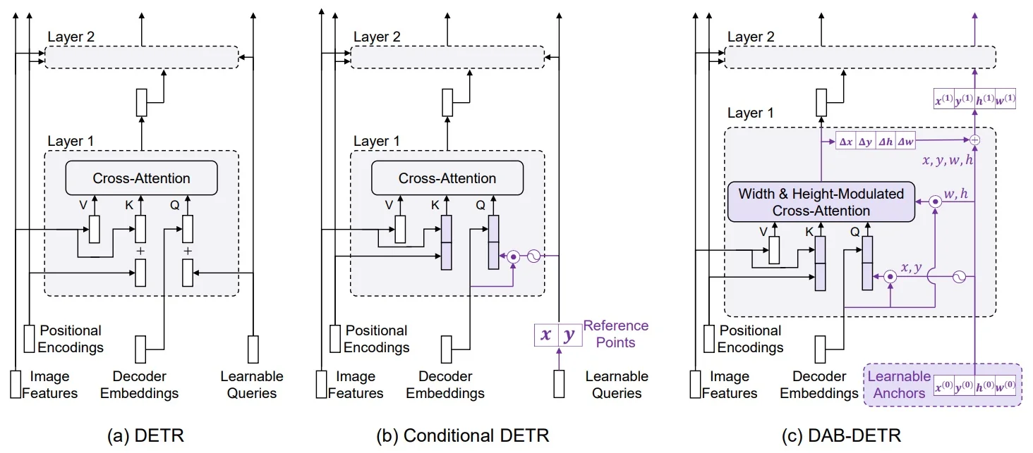
Architecturally, DAB-DETR preserves the DETR backbone–encoder–decoder layout.
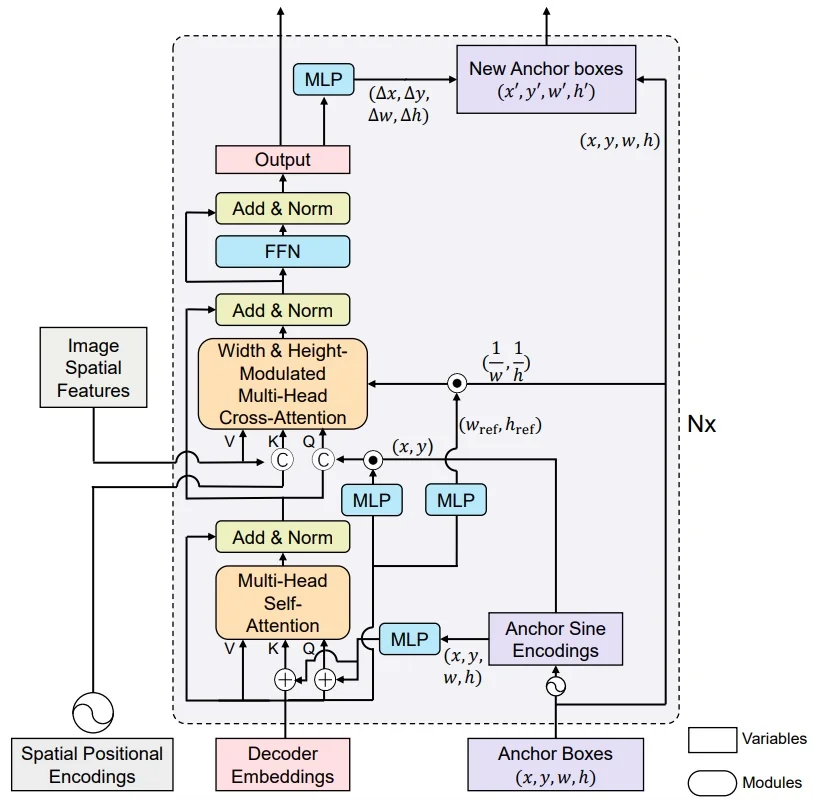
Nevertheless, it augments the decoder in two ways (as can be seen in the figure 15.47).
First, decoder queries are now pairs of content embeddings and dynamic anchors, with per-layer box heads that refine anchors via residual updates.
Second, multi-scale deformable cross-attention is parameterized by the current anchors: their centers define reference points from which a small set of sample locations is predicted and used to read from the multi-scale feature maps. The rest of the pipeline (backbone feature extraction, encoder processing of multi-scale features) remains unchanged.
For Mask DINO, this design is fundamental: the same dynamically refined anchors that make DAB-DETR and DINO-DETR queries geometrically well-localized for detection will later serve as strong spatial priors when those queries are reused for mask prediction.
DINO-DETR: improved denoising and query mechanics While DAB-DETR equips each query with a progressively refined anchor box and anchor-guided deformable attention, it still largely relies on randomly initialized query embeddings and a single, somewhat brittle training signal from the Hungarian-matched detection loss. DINO-DETR [337] builds directly on DAB-DETR and DN-DETR [338] to address these shortcomings. It preserves dynamic anchor boxes and multi-scale deformable cross-attention, but strengthens the training dynamics and query initialization via three key ideas:
- Contrastive denoising (CDN) to provide a stable, auxiliary reconstruction task that accelerates convergence and improves robustness.
- Mixed query selection that uses encoder outputs as data-dependent priors for decoder queries, avoiding purely “cold-start” learnable queries.
- A “look-forward-twice” box update mechanism that smooths the gradient path through the box regression heads and leads to more accurate localization.
Together, these make decoded queries not only well-localized (thanks to DAB-style anchors) but also semantically stronger and more robust—properties that Mask DINO will later exploit when reusing these queries for mask prediction.
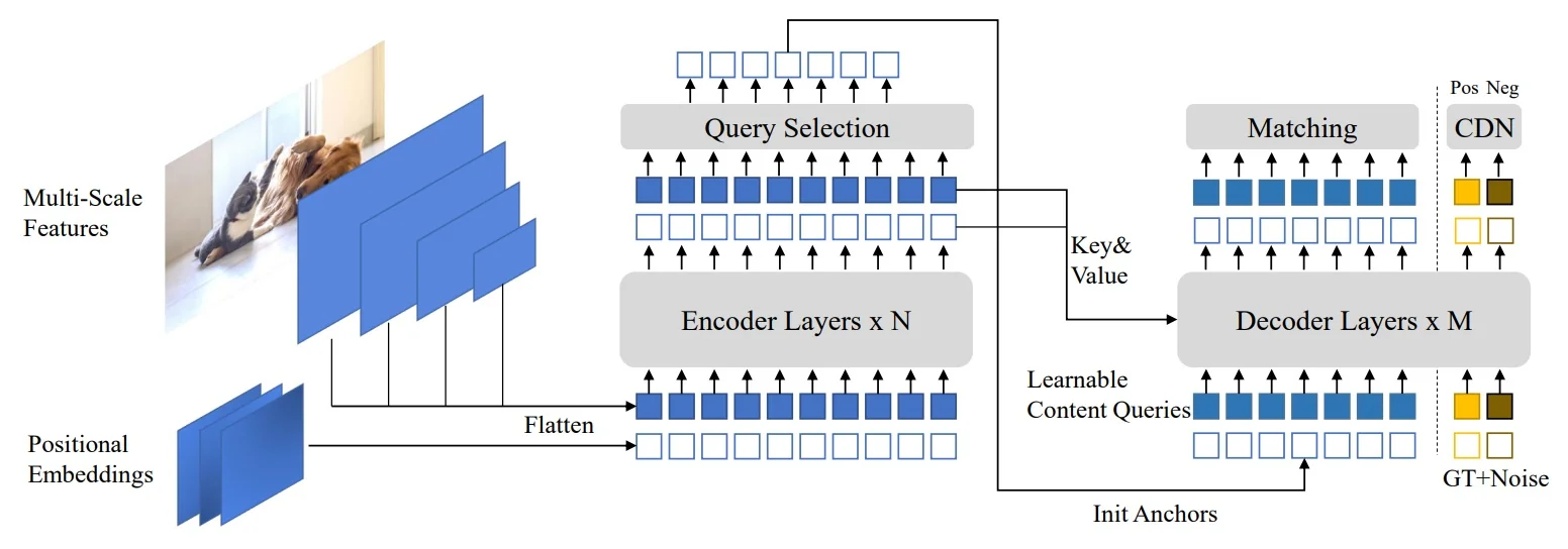
Contrastive denoising (CDN): a stable auxiliary objective In DETR-style models, the main supervision comes from Hungarian-matched predictions: each decoder layer produces a fixed set of queries, and a bipartite matching assigns some of them to ground-truth objects while the rest become “no object”. Early in training, when predictions are essentially random, this matching is unstable and gradients are noisy; queries receive weak, highly variable signals and learning is slow.
DN-DETR [338] and DINO-DETR [337] address this by adding a denoising branch alongside the usual “free” (detection) queries. The training queries are split into two groups:
- Detection queries, which behave as in standard DETR: they start from learned embeddings and anchors, are matched to ground truth via the Hungarian algorithm, and are trained to discover objects from scratch.
- Denoising queries, which are constructed directly from ground-truth box–label pairs and are trained to reconstruct the clean targets from corrupted versions.
Concretely, for each ground-truth box–label pair \((\mathbf {b}, c)\), the model samples one or more noised copies \[ \tilde {\mathbf {b}} = \mathbf {b} + \delta _{\mbox{box}}, \qquad \tilde {c} = c + \delta _{\mbox{cls}}, \] where \(\delta _{\mbox{box}}\) jitters the box center and size (within a controlled range) and \(\delta _{\mbox{cls}}\) may randomly flip the class to a nearby or “wrong” category. Each corrupted pair \((\tilde {\mathbf {b}}, \tilde {c})\) is then encoded as a denoising query (content embedding plus anchor initialized from \(\tilde {\mathbf {b}}\)) and passed through the same decoder as the detection queries. For these denoising queries, the supervision is direct: the loss compares their outputs to the clean ground-truth \((\mathbf {b}, c)\) from which they were generated, without any Hungarian matching.
This auxiliary task is intentionally easier than full detection: the model is told which approximate location and (possibly noisy) label to start from, and only needs to “pull” them back to the correct object. However, it does not leak information at inference time or make the overall problem trivial:
- At test time, there are no denoising queries and no ground-truth boxes; the decoder runs only on detection queries, which still must localize and classify objects from scratch using the standard detection loss.
- During training, detection and denoising queries share the same decoder weights and heads. Gradients from the denoising branch therefore shape the shared representation: they teach the decoder how to refine noisy, roughly located hypotheses into accurate boxes and labels, which directly benefits the harder detection queries once they start receiving meaningful matches.
- Because \(\tilde {\mathbf {b}}\) can be perturbed by different magnitudes and \(\tilde {c}\) can be corrupted, the model learns robustness to a range of geometric and semantic errors rather than memorizing exact ground-truth positions.
DINO-DETR further strengthens this idea with a contrastive formulation: denoising queries are organized so that each one is encouraged not only to match its own ground-truth target, but also to be clearly better (lower loss) for that target than for other ground truths in the same batch. This contrastive pressure sharpens the learned representation and reduces confusion between nearby objects.
Overall, the contrastive denoising (CDN) module supplies strong, stable gradients from the very beginning of training and makes queries robust to perturbations in both geometry and semantics. In the context of Mask DINO, these properties are crucial: when denoising is extended from boxes to masks, queries must learn to recover fine-grained shapes starting from noisy box-based hints, and CDN provides exactly the kind of robust refinement behavior that this requires.
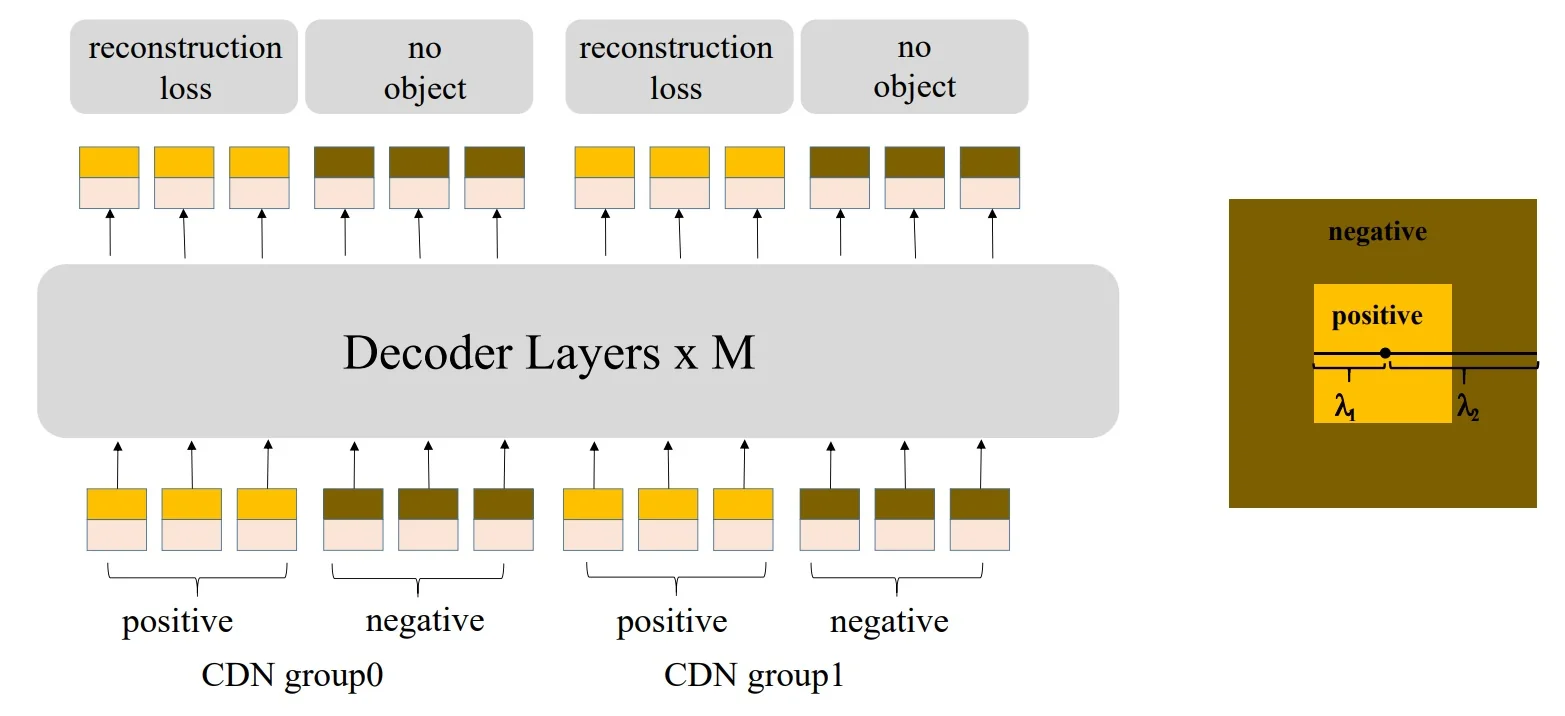
Mixed query selection: encoder priors for an image-aware warm start DAB-DETR equips each decoder query with a dynamic anchor, but the initial queries are still image-agnostic: at the first decoder layer they are generated from a fixed set of learned content embeddings and anchors that are identical for every image. The decoder must therefore discover, purely through end-to-end training, which queries should correspond to which objects in a new image. Early in training this leads to many queries drifting in empty background regions, unstable Hungarian matches, and slow convergence.
DINO-DETR [337] replaces this “cold start” by using the encoder as an image-specific proposal generator. After the encoder has processed the multi-scale features, we obtain a set of encoder tokens \[ \{e_j\}_{j=1}^{N_e}, \qquad e_j \in \mathbb {R}^d, \] indexed over all spatial locations and FPN levels. Lightweight heads are applied to these tokens to predict, for each \(e_j\),
- A classification score vector \(\hat {p}_j\) (probability over categories).
- A box prediction \(\hat {a}_j = (\hat {c}_{x,j}, \hat {c}_{y,j}, \hat {w}_j, \hat {h}_j)\).
These act as dense, coarse proposals: they tell us which encoder locations already look object-like and what rough boxes they suggest.
Mixed query selection then constructs the decoder’s initial queries from a mixture of these encoder proposals and a smaller pool of purely learned queries:
- 1.
- Score each encoder token \(e_j\) with a scalar objectness measure (for example, the maximum foreground class probability derived from \(\hat {p}_j\)).
- 2.
- Select the top \(K\) tokens according to this score; these are the encoder’s “hot spots” that are most likely to contain objects.
- 3.
- For each selected token \(e_j\):
- Use its feature \(e_j\) to initialize a decoder content query \(q^{(0)}_i\).
- Use its predicted box \(\hat {a}_j\) to initialize the associated anchor \(a^{(0)}_i\).
- 4.
- Fill the remaining decoder slots with a small number of image-agnostic learned queries (both content and anchors) to preserve flexibility and allow discovery of objects missed by the encoder proposals.
The result is that most decoder queries at layer 0 no longer start as generic, image-independent “slots” scattered over the feature maps. Instead, they are image-aware: their content embeddings and anchors are initialized from locations and appearances that the encoder already believes correspond to objects. The decoder’s role becomes primarily refinement: sharpen these coarse proposals, resolve overlaps and duplicates, and correct mistakes, rather than searching blindly over the entire image.
This has two concrete benefits:
- Faster and more stable training. From the very first epochs, many queries are already near true objects, so Hungarian matching becomes less random and gradients are less noisy. Empirically, this accelerates convergence and improves final box AP compared to starting all queries from learned, image-agnostic embeddings.
- Better queries for downstream tasks. Because the decoder refines proposals that already roughly localize objects, the resulting query embeddings tend to be semantically meaningful and spatially well grounded. For Mask DINO, which reuses these same queries for mask prediction, this is crucial: many queries that will later “paint” masks already correspond to plausible object candidates rather than arbitrary background locations.
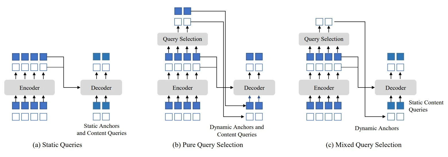
“Look-forward-twice” box updates: shorter gradient paths for better localization DAB-DETR already refines anchors layer by layer, but supervision for boxes is still relatively indirect: the strongest box losses are applied on the final decoder outputs, and their gradients must backpropagate through the entire stack of decoder layers and intermediate anchor updates. As depth grows, this long gradient path can weaken the learning signal reaching early layers, especially for the box regression branch, making it harder to steadily improve coarse localization.
DINO-DETR introduces a simple but effective modification, often described as “look-forward-twice”. At each decoder layer \(\ell \), the box head does not emit a single box prediction, but instead produces two closely related outputs for each query:
- an intermediate box \(\mathbf {b}_i^{\mbox{inter},(\ell )}\) that is used to update the anchor for the next layer, and
- a refined box \(\mathbf {b}_i^{\mbox{ref},(\ell )}\) that is supervised directly by the box regression loss.
The intermediate box preserves the residual refinement view introduced in DAB-DETR: it is added to the current anchor \(a_i^{(\ell )}\) to form the next-layer anchor \(a_i^{(\ell +1)} = a_i^{(\ell )} + \mathbf {b}_i^{\mbox{inter},(\ell )}\). The refined box, in contrast, is not fed forward but is explicitly compared to ground-truth boxes via the usual L1 and IoU-based losses at that decoder layer.
This dual prediction effectively creates a short, direct gradient path from the box loss at layer \(\ell \) back to the parameters of that layer’s box head and to its contributing query features. Instead of relying solely on losses applied at the very end of the decoder, every layer receives its own box-level supervision through \(\mathbf {b}_i^{\mbox{ref},(\ell )}\), while \(\mathbf {b}_i^{\mbox{inter},(\ell )}\) continues to drive the iterative anchor refinement. In practice, this improves gradient flow through the box regression branch, stabilizes training, and yields more accurate localization, particularly for small or thin objects where precise box edges matter.
For Mask DINO, this refinement is important because the same queries and anchors that benefit from DINO’s “look-forward-twice” design are later reused as spatial priors for mask prediction. Better-behaved, well-localized boxes mean that the queries start their mask prediction from anchors already close to the true object extent, so the subsequent mask head and pixel embedding map can focus on sharpening boundaries rather than compensating for large geometric errors.
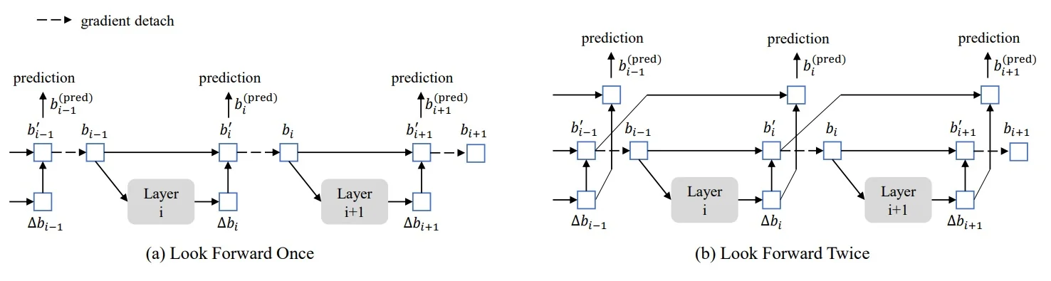
From Mask2Former to Mask DINO
The detection-oriented lineage culminating in DAB-DETR and DINO is built around box-savvy queries: each decoder query carries a dynamic 4D anchor box, and multi-scale deformable cross-attention lets it pull just enough context from a feature pyramid to localize objects with high-quality bounding boxes. However, segmentation requires more than tight boxes; it needs pixel-level shapes and boundaries. Mask2Former [100] attacks this problem from the opposite direction: it reinterprets queries as semantic projectors that “paint” dense masks over a high-resolution pixel embedding map via simple dot-products. Mask DINO is explicitly inspired by this idea and can be viewed as a fusion of DINO-DETR’s geometric machinery with Mask2Former’s unified, mask-centric segmentation pipeline.
Mask2Former: queries as semantic projectors for unified segmentation Mask2Former treats segmentation as set prediction over mask–class pairs, using a fixed set of abstract, learnable queries \[ Q = \{q_i\}_{i=1}^{N_q}, \qquad q_i \in \mathbb {R}^d. \] Each query \(q_i\) is a slot that is trained to represent one “thing” instance or one “stuff” region. The architecture has three tightly coupled components:
-
Backbone and pixel decoder: multi-scale pyramid and stride-4 pixel map. A CNN/ViT backbone first produces feature maps at several strides \[ \{F_s\}_{s \in \{4,8,16,32\}}, \qquad F_s \in \mathbb {R}^{C_s \times H/s \times W/s}, \] where \(s\) is the downsampling factor relative to the input resolution \(H \times W\). The pixel decoder (an FPN-style module) then:
- 1.
- Projects each backbone map to a common channel dimension \(d\) via \(1\times 1\) convolutions, giving \(\tilde F_s = W_s * F_s\).
- 2.
- Fuses them in a top-down manner: \[ G_{32} = \tilde F_{32}, \qquad G_s = \tilde F_s + \operatorname {Upsample}(G_{2s}) \quad (s=16,8,4), \] where \(\operatorname {Upsample}\) is typically bilinear upsampling to the spatial resolution of \(F_s\). This builds a coherent multi-scale pyramid \(\{G_s\}\) that combines high-level semantics (from coarse maps) with fine spatial detail (from shallow maps).
- 3.
- Optionally refines each \(G_s\) with multi-scale deformable attention (MS-DeformAttn) to obtain \(G_s'\): at every spatial location, MS-DeformAttn uses that location as a query and samples a small number of adaptive points across all scales, producing a content-adaptive blend of pyramid features with \(O(M)\) samples instead of \(O(HW)\) dense attention.
The finest refined map, which we denote \(G_4' \in \mathbb {R}^{H/4 \times W/4 \times d}\), is singled out as the pixel embedding map. In Mask2Former this is often written as \(F_4\); in the Mask DINO context we will later rename the same object to \(E\) to emphasize its role as a generic pixel embedding map. It lives at stride 4: high enough resolution to capture detailed boundaries, yet downsampled enough for efficient dense computation.
- Transformer decoder with masked attention: queries carve out regions. A Transformer decoder takes the query set \(Q\) and lets the queries iteratively refine themselves by attending to the multi-scale feature maps (typically the \(\{G_s'\}\)). The distinctive ingredient is masked cross-attention: at decoder layer \(\ell \), each query \(q_i^{(\ell )}\) is associated with a current estimated mask on the stride-4 grid. This mask is used to restrict the spatial positions that the query is allowed to attend to in the next cross-attention step. Intuitively, the query starts with a broad receptive field and, layer by layer, focuses its attention onto the pixels that it believes belong to its own region. This mechanism helps different queries specialize to different objects or stuff regions and stabilizes training by reducing interference between queries.
- Dot-product mask head: projecting queries onto the pixel map. After several decoder layers, each refined query \(\hat q_i\) is mapped through a small mask-embedding head to a vector \(\hat m_i \in \mathbb {R}^d\). The stride-4 pixel embedding map \(G_4'\) is treated as a dense grid of \(d\)-dimensional vectors. Mask logits are obtained by per-location dot-products: \[ \ell _i(x,y) = \langle \hat m_i, G_4'(x,y) \rangle , \qquad (x,y) \in \{1,\dots ,H/4\} \times \{1,\dots ,W/4\}, \] and then upsampled (typically bilinearly by a factor of 4) and passed through a sigmoid to produce a soft mask \[ m_i = \sigma \bigl (\operatorname {Upsample}(\ell _i)\bigr ) \in [0,1]^{H \times W}. \] In parallel, a classification head applied to \(\hat q_i\) predicts a semantic label \(c_i\). Geometrically, \(\hat m_i\) defines a direction in the \(d\)-dimensional embedding space; pixels whose embeddings \(G_4'(x,y)\) align with that direction receive high logit values and are included in the mask. The same set of \((c_i, m_i)\) pairs can be supervised as instance masks, panoptic segments, or semantic regions by changing only the loss and aggregation logic.
Putting these components together, the Mask2Former pipeline can be viewed as a coherent flow from raw pixels to mask–class pairs. An input image \[ I \in \mathbb {R}^{H \times W \times 3} \] is mapped by the backbone to a multi-scale feature pyramid \(\{F_s\}_{s \in \{4,8,16,32\}}\). The pixel decoder then reshapes this pyramid into a set of task-ready maps \(\{G_s'\}\) and, in particular, into a stride-4 pixel embedding map \(G_4' \in \mathbb {R}^{H/4 \times W/4 \times d}\) that serves as a dense, high-resolution canvas for segmentation.
A fixed set of queries \(Q\) enters the Transformer decoder, where masked cross-attention lets each query iteratively carve out its own region by repeatedly attending to \(\{G_s'\}\) under the guidance of its current mask. After several layers, the refined queries are converted into mask embeddings, and a simple dot-product between each mask embedding and the stride-4 pixel map \(G_4'\) produces low-resolution mask logits, which are finally upsampled and thresholded to yield full-resolution masks \(m_i(x,y)\), with a parallel head predicting class labels \(c_i\).
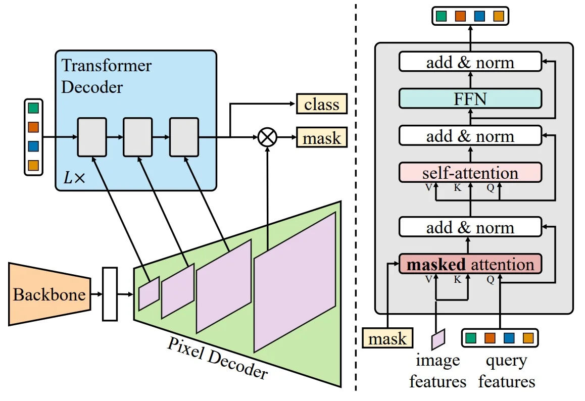
From the perspective of DAB-DETR and DINO-DETR, Mask2Former innovates by densifying the prediction pipeline. Rather than equipping queries with explicit 4D anchors and training them primarily to regress boxes in \(\mathbb {R}^4\), it reallocates capacity toward:
- A strong pixel decoder that builds a high-quality multi-scale pyramid and a stride-4 pixel embedding map suited to pixel-level decisions.
- MS-DeformAttn-based multi-scale fusion inside the pixel decoder, which allows each spatial location to aggregate a small number of informative samples across all scales instead of performing dense attention over all positions, and
- A dot-product mask head that treats each query (after a small mask-embedding MLP) as a semantic direction in the embedding space and uses that direction to assign labels to pixels on the stride-4 grid.
In this formulation, queries are no longer geometric anchors tied to 4D boxes; they are semantic projectors that decide which pixels on a high-resolution embedding canvas belong to which region.
The architectural gap between DINO-DETR/DAB-DETR and Mask2Former Despite sharing many underlying components (CNN/ViT backbones, multi-scale pyramids, Transformer encoders/decoders), the two families crystallize around different objectives and therefore make different design choices:
- DINO-DETR and DAB-DETR: box-first, sparse geometry. Decoder queries carry dynamic 4D anchor boxes and interact with features via multi-scale deformable attention guided by reference points. Training emphasizes accurate box regression and classification, supported by contrastive denoising, mixed query selection, and per-layer box refinement. There is no pixel decoder producing a dedicated stride-4 embedding map for masks, no dot-product mask head, and no mechanism to turn each query into a dense mask \(m_i(x,y)\) over the image plane.
- Mask2Former: mask-first, dense semantics. Decoder queries are purely semantic (DETR-style content plus positional encodings) and do not maintain explicit 4D anchors. Masked attention and the pixel decoder are optimized to refine masks on the stride-4 grid, not to iteratively refine bounding boxes. As a result, Mask2Former achieves state-of-the-art segmentation quality, but its box localization lags behind anchor-based detectors such as DINO-DETR and DAB-DETR: it lacks dynamic anchors, per-layer box updates, and a denoising scheme tailored to box regression.
These contrasting design commitments create a clear architectural gap. DINO-DETR and DAB-DETR provide robust, geometry-aware queries and excellent box predictions but no dense mask head, whereas Mask2Former provides an elegant, unified mask-prediction pipeline but weaker geometric priors for boxes. Mask DINO is motivated precisely by this complementarity and will fuse DINO-DETR’s box-savvy queries with a Mask2Former-style pixel decoder and dot-product mask head so that a single set of queries can jointly support detection and segmentation in the form of \((c_i, \mathbf {b}_i, m_i)\) tuples.
Mask DINO: DINO-DETR queries as Mask2Former-style projectors Mask DINO closes the gap between box-first DINO-DETR and mask-first Mask2Former by reusing DINO-DETR’s detection-strength queries as Mask2Former-style semantic projectors on a stride-4 pixel embedding map. Conceptually, the architecture keeps the entire DINO-DETR detector intact, and attaches a Mask2Former-inspired segmentation branch that interprets the same decoder content queries as directions in a dense embedding space.
At a high level, the end-to-end flow for an input image \[ I \in \mathbb {R}^{H_0 \times W_0 \times 3} \] is as follows:
- DINO-DETR backbone, encoder, and decoder (detection part, “blue”). As in DINO-DETR, a CNN/ViT backbone produces multi-scale features, which are consumed by a multi-scale deformable Transformer encoder. Unified query selection uses encoder heads to pick high-quality object priors and initialize decoder queries with dynamic anchor boxes. A stacked decoder with multi-scale deformable cross-attention, contrastive denoising, mixed query selection, and “look-forward-twice” box refinement converts these into a refined set of content queries \[ Q^{\mbox{dec}} = \{q_i\}_{i=1}^{N_q}, \qquad q_i \in \mathbb {R}^d, \] along with their associated anchors. Per-query class and box heads (inherited from DINO-DETR) predict logits \(c_i\) and 4D boxes \(\mathbf {b}_i\), preserving state-of-the-art detection performance.
- Mask2Former-style pixel decoder and pixel embedding map (segmentation canvas, “red”). In parallel, a pixel decoder (as in Mask2Former) fuses backbone (and optionally encoder) features into a refined multi-scale pyramid \(\{G'_s\}_{s \in \{32,16,8,4\}}\). Its stride-4 output \[ E \equiv G'_4 \in \mathbb {R}^{H_4 \times W_4 \times d}, \qquad H_4 = \frac {H_0}{4}, \; W_4 = \frac {W_0}{4}, \] serves as the pixel embedding map: each location \((x,y)\) holds a \(d\)-dimensional embedding \(E(x,y)\) summarizing local appearance and context at stride 4. Subsequent subsections will refine this description and show how \(E\) is constructed from backbone and encoder features.
- Dot-product mask head driven by DINO queries (segmentation part, “red”). The same refined decoder content queries \(q_i\) that feed the detection heads are reinterpreted as mask projectors. A light mask-embedding head maps \(q_i\) to a mask vector \(\hat m_i \in \mathbb {R}^d\), and mask logits at stride 4 are obtained by per-location dot-products \[ \ell _i(x,y) = \langle \hat m_i, E(x,y) \rangle , \qquad (x,y) \in \{1,\dots ,H_4\} \times \{1,\dots ,W_4\}, \] followed by upsampling (typically bilinear \(\times 4\)) and a sigmoid to produce a full-resolution mask \[ m_i = \sigma \bigl (\operatorname {Upsample}(\ell _i)\bigr ) \in [0,1]^{H_0 \times W_0}. \] Thus, each single query \(q_i\) now produces a triplet \((c_i, \mathbf {b}_i, m_i)\): a class, a bounding box, and a dense mask.
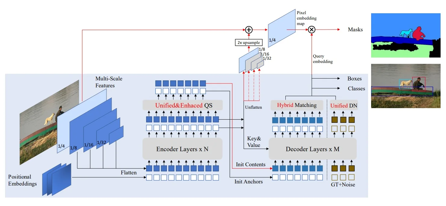
Mask DINO further extends DINO-DETR’s encoder heads, denoising scheme, and Hungarian matching cost so that boxes and masks are selected, denoised, and matched jointly rather than in separate pipelines: encoder heads output both box and mask scores for unified query selection; denoising operates on noised box–label and mask targets; and the matching cost combines classification, box, and mask terms. In effect, DINO-DETR’s geometry-aware query engine provides precise localization priors, while Mask2Former’s pixel decoder and dot-product head turn those same queries into powerful mask projectors on a stride-4 embedding canvas.
This unified design preserves the geometric rigor of DINO-DETR (dynamic anchors, multi-scale deformable attention, denoising, mixed query selection) while importing Mask2Former’s core insight that queries can be turned into semantic projectors via dot-products with a stride-4 pixel embedding map. The remainder of this section unpacks each component in detail, starting from the backbone and multi-scale features and moving through the pixel decoder, encoder and decoder design, and the segmentation branch and training losses.
Backbone and Multi-Scale Features
Mask DINO uses a CNN or ViT backbone (e.g., ResNet-50, Swin-L) to produce multi-scale feature maps \[ \{F_{32}, F_{16}, F_{8}, F_{4}\}, \] where the subscript denotes the stride relative to the input resolution. Each map has shape \[ F_s \in \mathbb {R}^{C_s \times H_s \times W_s}, \qquad H_s = \frac {H_0}{s}, \; W_s = \frac {W_0}{s}. \]
A pixel decoder (inherited from Mask2Former) then transforms these backbone features into a refined pyramid \[ \{\tilde F_s\}_{s \in \{32,16,8,4\}}, \quad \{G_s\}_{s \in \{32,16,8,4\}}, \quad \{G'_s\}_{s \in \{32,16,8,4\}}, \] where:
- \(\tilde F_s\) are lateral projections to a common dimensionality \(d\).
- \(G_s\) are FPN-style top–down fused features.
- \(G'_s\) are refined features produced by multi-scale deformable attention.
Formally, a \(1\times 1\) convolution \[ \tilde F_s = W_s^{\mbox{lat}} * F_s, \qquad W_s^{\mbox{lat}} \in \mathbb {R}^{d \times C_s \times 1 \times 1}, \] projects each \(F_s\) into a \(d\)-dimensional feature space without changing spatial resolution. A top–down FPN fusion then constructs \[ G_{32} = \tilde F_{32}, \quad G_{16} = \tilde F_{16} + \operatorname {Upsample}(G_{32}), \quad G_{8} = \tilde F_{8} + \operatorname {Upsample}(G_{16}), \quad G_{4} = \tilde F_{4} + \operatorname {Upsample}(G_{8}), \] where \(\operatorname {Upsample}\) is typically stride-2 bilinear interpolation to match the spatial size of the next finer scale.
Finally, each \(G_s\) is refined by multi-scale deformable attention (MS-DeformAttn) to obtain \(G'_s\). The coarser levels \(G'_8, G'_{16}, G'_{32}\) are then fed into the Transformer encoder as multi-scale inputs, while the pixel embedding map will later be constructed separately from the stride-4 backbone feature \(C_b\) and the stride-8 encoder feature \(C_e\).
Multi-Scale Deformable Attention in the Pixel Decoder
Mask DINO (via Mask2Former) uses MS-DeformAttn [827] both in the encoder and in the pixel decoder. This subsection focuses on the pixel decoder refinement \[ G_s \;\longrightarrow \; G'_s, \] and explains how queries, keys, values, sampling locations, and attention weights are defined.
Standard global attention (reminder) In standard dot-product attention, we have \[ Q \in \mathbb {R}^{N_q \times d}, \quad K, V \in \mathbb {R}^{N_k \times d}, \] and \begin {equation} \operatorname {Attn}(Q,K,V) = \operatorname {softmax}\!\left (\frac {QK^\top }{\sqrt {d}}\right )V. \label {eq:chapter15_maskdino_standard_attn} \end {equation} For a single query \(q \in \mathbb {R}^d\), this reads \[ \alpha _j = \frac {\exp (\langle q,k_j\rangle / \sqrt {d})}{\sum _{j'} \exp (\langle q,k_{j'}\rangle / \sqrt {d})}, \qquad \operatorname {Attn}(q,K,V) = \sum _j \alpha _j v_j. \] Each query attends densely to all \(N_k\) keys/values, which is too expensive when \(K,V\) come from large feature maps.
High-level idea of MS-DeformAttn MS-DeformAttn replaces dense global attention by:
- Sparse attention: each query attends to \(M\) sampling locations per head instead of all spatial positions.
- Multi-scale attention: those sampling locations span multiple pyramid levels (e.g., strides \(4,8,16,32\)).
- Content-adaptive attention: sampling locations and their weights are predicted from the query itself.
Instead of computing all dot products \(\langle q,k_j\rangle \), the module:
- 1.
- Predicts where to look (sampling offsets) from the query \(q_p\).
- 2.
- Samples values \(V_{s'}\) at those locations across scales.
- 3.
- Predicts how strongly to weight each sample from \(q_p\) via a small linear layer.
There is no explicit dense set of keys; the query implicitly defines both the sampling locations and the pattern in which sampled values are mixed.
Inputs to MS-DeformAttn in the pixel decoder Fix a scale \(s \in \{4,8,16,32\}\). The inputs are:
- Queries. The query features are the current fused map \[ Q_s = G_s \in \mathbb {R}^{d \times H_s \times W_s}, \] flattened into \(Q_s^{\mbox{flat}} \in \mathbb {R}^{(H_s W_s) \times d}\). Each spatial position \(p=(i,j)\) corresponds to a query vector \[ q_p = G_s(i,j) \in \mathbb {R}^d. \]
- Keys and values. Keys and values are all laterally projected backbone features \[ \mathcal {F} = \{\tilde F_{4}, \tilde F_{8}, \tilde F_{16}, \tilde F_{32}\}, \] with \(K_{s'} = V_{s'} = \tilde F_{s'}\) for each scale \(s'\). These are flattened per scale but are conceptually kept as separate feature maps.
- Reference points. Each spatial position \(p=(i,j)\) at scale \(s\) has a normalized reference coordinate \[ r_p = \left (\frac {j}{W_s}, \frac {i}{H_s}\right ) \in [0,1]^2, \] indicating where in the image this query lives.
Step-by-step computation for a single query Fix a scale \(s\), a spatial position \(p\), a head index \(h \in \{1,\dots ,H\}\), and a sampling index \(m \in \{1,\dots ,M\}\).
(1) Sampling offsets. From the query \(q_p\) we predict a 2D offset \[ \Delta _{h,m}(p) = W^{\Delta }_{h,m} q_p \in \mathbb {R}^2, \] where \(W^{\Delta }_{h,m} \in \mathbb {R}^{2 \times d}\) is a learned matrix. This offset specifies how far, and in what direction, to move from the reference point \(r_p\).
(2) Sampling locations. The normalized sampling location is \begin {equation} \phi _{h,m}(p) = r_p + \Delta _{h,m}(p) \in \mathbb {R}^2. \label {eq:chapter15_maskdino_sampling} \end {equation} \(\phi _{h,m}(p)\) is continuous and may fall between pixels. Each sampling point is also associated with a scale \(s'_{h,m} \in \{4,8,16,32\}\) (in practice, each head has a fixed or learned pattern for how its \(M\) samples are distributed across scales).
(3) Sampling values from multi-scale features. At the chosen scale \(s'_{h,m}\), the location \(\phi _{h,m}(p)\) is interpreted in that feature map’s coordinate frame, and a value vector is obtained via bilinear interpolation: \[ v_{h,m}(p) = V_{s'_{h,m}}\bigl (\phi _{h,m}(p)\bigr ) \in \mathbb {R}^d. \]
(4) Unnormalized attention scores. For each sample we compute a scalar logit \[ w_{h,m}(p) = u_{h,m}^\top q_p, \] where \(u_{h,m} \in \mathbb {R}^d\) is a learned vector (or a row of a small linear layer). This plays a role analogous to \(\langle q,k_j\rangle \) in standard attention: it scores how much the query wants to use the \(m\)-th sample for head \(h\).
(5) Attention weights. For fixed \(h\) and \(p\), these logits are normalized across \(m\): \[ A_{h,m}(p) = \frac {\exp (w_{h,m}(p))}{\sum _{m'=1}^M \exp \bigl (w_{h,m'}(p)\bigr )}. \] The weights \(\{A_{h,m}(p)\}_{m=1}^M\) form a convex combination over the sampled values \(\{v_{h,m}(p)\}_{m=1}^M\) and are the sparse analogue of the softmax over all keys in (15.2). The form is chosen to provide:
- Smooth, differentiable importance scores.
- Normalization to control magnitude.
- Content-adaptive weighting of a small learned set of sampling points.
(6) Head output and multi-head output. Each head combines its sampled values as \[ \operatorname {head}_h(q_p) = \sum _{m=1}^M A_{h,m}(p)\, W_h v_{h,m}(p), \] where \(W_h \in \mathbb {R}^{d_h \times d}\) is a learned projection and \(\sum _h d_h = d\). The multi-head output is then \[ \operatorname {MSDeformAttn}(q_p) = \operatorname {Concat}_{h=1}^H \operatorname {head}_h(q_p) \in \mathbb {R}^d. \]
Residual refinement of \(G_s\) At each scale \(s\), MS-DeformAttn produces a refined feature for each position \(p\) via a residual update: \begin {equation} G'_s(p) = G_s(p) + \operatorname {MSDeformAttn}\!\bigl ( q_p, \{\tilde F_{s'}\}_{s' \in \{4,8,16,32\}} \bigr ), \quad q_p = G_s(p). \label {eq:chapter15_maskdino_msdeform_update} \end {equation} Thus every scale \(s \in \{4,8,16,32\}\) is refined into \(G'_s\).
Why weights depend only on the query In standard attention, weights are \(\alpha _j \propto \exp (\langle q,k_j\rangle )\). Here, we do not explicitly maintain a dense set of keys \(k_j\):
- The choice of where to sample is already conditioned on the query via \(\Delta _{h,m}(p)\) and \(\phi _{h,m}(p)\).
- The content at those positions is captured in \(v_{h,m}(p)\).
- We only need a relative ranking among the \(M\) samples for each head and position.
The simple bilinear form \[ w_{h,m}(p) = u_{h,m}^\top q_p \] is thus sufficient and efficient: the query chooses a pattern, offsets choose where to look, values encode what is found, and attention weights decide how to mix the sampled patterns.
Cross-attention vs. self-attention In the pixel decoder:
- Queries are the fused features \(G_s\) (or \(G'_s\)) at a given scale.
- Keys and values are the multi-scale backbone features \(\{\tilde F_{s'}\}_{s' \in \{4,8,16,32\}}\).
Here MS-DeformAttn acts as multi-scale cross-attention: fused features at scale \(s\) attend sparsely to the backbone pyramid.
In the Transformer encoder, queries, keys, and values all come from the same multi-scale set of encoder features, so MS-DeformAttn plays the role of multi-scale self-attention, analogous to the encoder in Deformable DETR [827].
In the Transformer decoder, queries are the object queries and keys/values are the encoder’s multi-scale outputs, so MS-DeformAttn again acts as multi-scale cross-attention from queries to the encoder memory.
Why all scales \(G'_s\) must be refined Although only the stride-4 refined map \(G'_4\) is directly used to build the pixel embedding map, Mask DINO refines every scale \(s\in \{4,8,16,32\}\):
- The FPN fusion is top–down: \(G_4\) depends on \(G_8\), which depends on \(G_{16}\), and so on. If coarse maps are unrefined, noise and misalignment propagate down.
- MS-DeformAttn at scale \(4\) samples from all scales \(\tilde F_{s'}\). If those maps are not semantically clean, the sampling locations and values seen by \(G'_4\) will be inconsistent.
- Coarse scales carry global semantic and shape information; refining them first ensures that when \(G'_4\) samples them, it receives coherent context rather than raw backbone features.
In short, a clean stride-4 representation cannot be built by sampling from unrefined coarse maps; therefore all \(G_s\) must be refined into \(G'_s\) before \(G'_4\) can serve as a high-quality pixel embedding map.
Transformer Encoder and Decoder in Mask DINO
Up to this point we have taken an input image \[ I \in \mathbb {R}^{H_0 \times W_0 \times 3} \] through a backbone and pixel decoder to obtain a refined multi-scale pyramid \[ \{G_s'\}_{s \in \{4,8,16,32\}}, \qquad G_s' \in \mathbb {R}^{d \times H_s \times W_s}, \quad H_s = \tfrac {H_0}{s},\; W_s = \tfrac {W_0}{s}. \] For a typical COCO-style input of \(H_0 \approx 800\), \(W_0 \approx 1333\), the finest map \(G_4'\) has resolution \(H_4 \approx 200\), \(W_4 \approx 333\), while \(G_{32}'\) is much coarser but carries strong semantic context. You can think of \(\{G_s'\}\) as a multi-scale canvas where each location already encodes a blend of local detail and global context thanks to MS-DeformAttn in the pixel decoder.
Mask DINO now feeds these features into a DINO-style encoder–decoder to produce a set of refined, box-savvy queries that will later drive both bounding boxes and masks. The goal of this stage is: given the refined pyramid \(\{G_s'\}\), identify a small set of promising object candidates and iteratively refine them into high-quality query embeddings \(\hat q_i\) that can support joint \((c_i,\mathbf {b}_i,m_i)\) prediction.
Encoder: from refined pyramid to token proposals With the pixel decoder in place, we start the Transformer stage from the refined multi-scale pyramid \[ \{G_s'\}_{s \in \{4,8,16,32\}}, \qquad G_s' \in \mathbb {R}^{d \times H_s \times W_s}, \quad H_s = \tfrac {H_0}{s},\; W_s = \tfrac {W_0}{s}. \] Mask DINO follows DINO and runs the encoder on the three coarser pyramid levels, typically \(s \in \{8,16,32\}\), while the stride-4 map is reserved for constructing the pixel embedding map. Coarse levels provide global semantics and rough shapes, whereas the finest encoder level (\(s = 8\)) carries more detailed edges and boundaries; the encoder’s job is to let every location see just enough of both.
Concretely, the encoder follows DINO-DETR but replaces dense self-attention with MS-DeformAttn:
- Each \(G_s'\) is flattened into a sequence of tokens \[ T_s \in \mathbb {R}^{(H_s W_s) \times d}, \] and all scales are processed jointly through \(L_{\mbox{enc}}\) layers of MS-DeformAttn-based self-attention and feed-forward networks, yielding encoder outputs \(E_{e,s} \in \mathbb {R}^{(H_s W_s) \times d}\) at each scale.
- In each MS-DeformAttn layer, the queries are the current tokens at positions \(p\) on each \(G_s'\), while the keys and values come from the entire multi-scale set \(\{G_{s'}'\}_{s' \in \{4,8,16,32\}}\) treated as a single multi-scale memory. For a token \(q_p\) at position \(p\) on level \(s\), the module predicts a small set of offsets and scales, samples a few values from nearby and cross-scale positions (via bilinear interpolation), and mixes them with learned attention weights, exactly as in the MS-DeformAttn formulation described earlier.
- The effect is that each encoder token becomes a context-aware descriptor: a location on \(G_4'\) near a dog’s ear can pull in coarse information from \(G_{32}'\) about the overall dog silhouette and complementary detail from \(G_8'\) or \(G_{16}'\), without paying the cost of dense global attention.
On top of these encoder outputs, Mask DINO attaches three lightweight heads that turn tokens into dense proposals:
- A classification head that predicts how likely each token is to correspond to a foreground object instance or a stuff region.
- A box head that predicts a coarse 4D bounding box for each token, typically as normalized coordinates or offsets relative to its spatial location.
- A mask head that predicts a coarse mask for each token by projecting its embedding onto the stride-4 pixel embedding map \(E\) (constructed in the pixel-decoder branch) via a dot-product, producing early mask logits on the \(H_4 \times W_4\) grid.
For every encoder token, this yields an early triplet \((\hat c,\hat {\mathbf {b}},\hat m)\). Intuitively, the encoder behaves like a dense proposal generator. Given the refined pyramid, it produces a heatmap of “interesting” locations and associated coarse boxes and masks. For example, in an image containing a dog and a person, tokens around the dog’s torso will tend to have high “dog” scores, a roughly dog-shaped mask, and a bounding box enclosing the dog; tokens near the person will produce analogous proposals for the person. Mask DINO will not keep all of these dense proposals; instead, it uses them to initialize a much smaller set of decoder queries.
Unified query selection: seeding decoder queries and anchors Rather than starting decoder queries from purely learned embeddings, Mask DINO adopts DINO’s unified query selection and extends it to take mask quality into account. The idea is to select a small number of the most promising encoder tokens and turn them into decoder queries with good initial content and good initial anchor boxes.
For each encoder token, Mask DINO attaches three prediction heads that share their architecture with the decoder heads. In practice:
- The classification head outputs a foreground class score. This score alone is used to rank encoder tokens and select the top-ranked features to become decoder content queries.
- The box head predicts a coarse 4D box for each token. These boxes are supervised with the standard detection loss and will become initial anchors for the decoder.
- The mask head predicts a coarse mask for each token by dot-producting the token with the high-resolution pixel embedding map \(E\), and is supervised with a mask loss. These coarse masks are also used to derive tighter boxes that better follow the object support.
During unified query selection, Mask DINO simply takes the top \(N_q\) encoder tokens by classification confidence, uses their encoder features as the initial content embeddings \(q_i^{(0)}\), and uses the associated predicted boxes (optionally refined using the coarse masks) as the initial anchor boxes \(a_i^{(0)}\). This matches the “unified and enhanced query selection” design in the paper: the three heads provide detection and segmentation priors on encoder tokens, but the classification score drives ranking, while the predicted boxes and masks supply supervised initial anchors for the decoder.
Mask DINO then:
- Selects the top \(N_q\) encoder tokens according to this unified score (optionally mixing in a small number of learned queries for robustness).
-
Uses the selected encoder features as the initial content embeddings of decoder queries \(q_i^{(0)}\).
- Uses the selected boxes (often refined using the corresponding coarse masks to better fit object extent) as the initial anchor boxes \(a_i^{(0)}\) for those queries.
This step converts a dense field of thousands of encoder tokens into a compact set of \(N_q\) object candidates that are already biased toward good shapes. Because masks are usually easier to learn than precise boxes early in training (pixel-level supervision provides many more gradients than sparse box corners), the encoder mask head often provides the most reliable early signal. Mask DINO exploits this by effectively performing mask-enhanced anchor box initialization: boxes derived from regions with good masks provide stronger geometric priors for the decoder than boxes coming from box regression alone.
Decoder: from proposals to refined box-aware queries The decoder then refines these \(N_q\) selected queries using the DINO-DETR design, but now with the added role of supporting mask prediction. Each decoder query carries two coupled components: a content embedding \(q_i^{(\ell )} \in \mathbb {R}^d\) and an anchor box \(a_i^{(\ell )} \in \mathbb {R}^4\) at layer \(\ell \).
At a high level, each decoder layer performs three standard Transformer operations, plus per-layer prediction heads:
- Self-attention over the current set of queries so that different queries can exchange information and resolve competition when they cover overlapping regions.
- Multi-scale deformable cross-attention from queries to the encoder outputs \(\{E_{e,s}\}\), using the current anchor box \(a_i^{(\ell )}\) of each query to define its reference points for MS-DeformAttn. For query \(i\), the center of \(a_i^{(\ell )}\) is normalized and used as the reference; the module then predicts a small set of offsets and scales, samples values from nearby positions across all scales, and aggregates them to update \(q_i^{(\ell )}\). This allows each query to pull just the relevant context from the refined pyramid, focusing on its hypothesized object region.
- A position-wise feed-forward network (FFN) that further refines the updated query embeddings.
As in DINO-DETR, each decoder layer also has prediction heads:
- A classification head that predicts class scores from the current query embedding \(q_i^{(\ell )}\).
- A box head that predicts both intermediate and refined boxes from \(q_i^{(\ell )}\), enabling the “look-forward-twice” mechanism where intermediate boxes become the anchors \(a_i^{(\ell +1)}\) for the next layer, and refined boxes are directly supervised.
Mask DINO adds:
- A decoder mask head that predicts a mask for each query at selected layers by projecting \(q_i^{(\ell )}\) onto the stride-4 pixel embedding map \(E\) via a dot-product, providing additional shape-focused supervision while boxes are still being refined.
After \(L_{\mbox{dec}}\) decoder layers, we obtain a final set of refined content queries \[ \hat Q = \{\hat q_i\}_{i=1}^{N_q}, \qquad \hat q_i \in \mathbb {R}^d, \] together with their associated refined anchor boxes and the per-layer predictions from intermediate heads. Each \(\hat q_i\) can be viewed as a compact description of one predicted object or stuff region: it has been geometrically grounded via dynamic anchors and multi-scale deformable attention, and semantically shaped by both box and mask supervision. These refined queries are then passed to the final classification, box, and mask heads described in the next part to produce the model’s \((c_i,\mathbf {b}_i,m_i)\) outputs.
Segmentation Branch and Pixel Embedding Map
The segmentation branch turns refined queries \(\hat q_i\) into dense masks by projecting them onto a stride-4 pixel embedding map, in the spirit of Mask2Former. Conceptually, this is where DINO’s box-savvy queries become Mask2Former-style semantic projectors.
Constructing the pixel embedding map Mask DINO constructs a stride-4 pixel embedding map by fusing backbone and encoder features. Let:
- \(C_b \in \mathbb {R}^{C_b \times H_4 \times W_4}\) be the stride-4 feature map from the backbone.
- \(C_e \in \mathbb {R}^{d \times H_8 \times W_8}\) be an encoder feature at stride \(8\), obtained by reshaping the corresponding encoder tokens \(E_{e,8}\).
- \(T\) be a \(1\times 1\) convolution mapping \(C_b\) to the Transformer hidden dimension \(d\).
- \(F\) be a \(2\times \) upsampling operation that brings \(C_e\) from stride \(8\) to stride \(4\) via bilinear interpolation.
- \(M\) be a lightweight segmentation head (for example, a few \(3\times 3\) convolutions with normalization and nonlinearity) operating on stride-4 features.
The fused pixel embedding map is then \begin {equation} E(x,y) = M\bigl (T(C_b)(x,y) + F(C_e)(x,y)\bigr ) \in \mathbb {R}^d, \label {eq:chapter15_maskdino_pixel_map} \end {equation} for \((x,y)\) on the stride-4 grid \((H_4 \times W_4)\). Intuitively, \(T(C_b)\) contributes high-resolution local detail (edges, textures) while \(F(C_e)\) injects encoder-level context (which object is likely present at that location). The head \(M\) mixes these signals into a per-pixel embedding \(E(x,y)\) that is well-suited for deciding “which object or region this pixel belongs to.”
Query–pixel dot products as mask logits Each refined decoder content query \(\hat q_i \in \mathbb {R}^d\) is then turned into a mask by a simple dot-product with the pixel embedding map. Formally, the implementation applies a small linear layer to produce a mask embedding \(\hat m_i \in \mathbb {R}^d\) and uses \[ \ell _i(x,y) = \langle \hat m_i, E(x,y) \rangle , \qquad (x,y) \in \{1,\dots ,H_4\} \times \{1,\dots ,W_4\}. \] These \(\ell _i\) are stride-4 mask logits, which are then upsampled to the input resolution and passed through a sigmoid: \[ m_i = \sigma \bigl (\operatorname {Upsample}(\ell _i)\bigr ) \in [0,1]^{H_0 \times W_0}. \]
Geometrically, \(\hat m_i\) defines a direction in the \(d\)-dimensional embedding space. Pixels whose embeddings \(E(x,y)\) align strongly with \(\hat m_i\) receive large positive logits and are included in the mask. For example, if \(\hat q_i\) has learned to represent “this particular dog instance”, then \(E(x,y)\) at the dog’s pixels will be close to \(\hat m_i\), and \(\ell _i(x,y)\) will be high there, while background pixels will have low logits. This is exactly the Mask2Former mechanism, now driven by DINO-style queries.
In parallel, the same \(\hat q_i\) is fed to the class and box heads inherited from DINO-DETR to predict \[ c_i \in \mathbb {R}^{C+1}, \qquad \mathbf {b}_i \in \mathbb {R}^4. \] The crucial point is that the same query representation \(\hat q_i\) is responsible for all three outputs \((c_i,\mathbf {b}_i,m_i)\). Box and mask supervision therefore shape a shared representation rather than training two disjoint branches. In practice this improves both detection and segmentation: better masks help the model learn tighter boxes, and better boxes help the model focus its mask predictions.
Unified Denoising and Hybrid Matching
The final piece is how Mask DINO trains this unified architecture so that queries become simultaneously good classifiers, localizers, and mask projectors.
Extending denoising from boxes to masks DINO-DETR uses contrastive denoising: extra decoder queries are reserved for reconstructing ground-truth boxes and labels from noised versions of those targets. This stabilizes training and accelerates convergence for detection. Mask DINO extends this idea to segmentation:
- Ground-truth boxes and masks are perturbed, for example by jittering box coordinates or slightly eroding/dilating masks, to generate noisy training targets.
- A subset of decoder queries is dedicated to reconstructing the original boxes and masks from these noised targets, in addition to the standard detection denoising.
Because masks carry finer-grained information than boxes, this mask-aware denoising provides strong gradients that encourage queries to capture detailed object shapes early in training. For a dog example, even if the initial box roughly covers the dog and some background, the denoising loss forces the query to predict a mask that tightly follows the dog’s silhouette, which in turn helps refine the box in later decoder layers. Empirically, this leads to faster convergence and better mask quality.
Hybrid matching cost for joint detection and segmentation As in other DETR-style models, Mask DINO uses the Hungarian algorithm to match predicted queries to ground-truth instances. The key difference is that the matching cost combines classification, box, and mask terms: \[ L_{\mbox{match}} = \lambda _{\mbox{cls}} L_{\mbox{cls}} + \lambda _{\mbox{box}} L_{\mbox{box}} + \lambda _{\mbox{mask}} L_{\mbox{mask}}. \] Here \(L_{\mbox{cls}}\) is a classification loss (for example cross-entropy or focal loss), \(L_{\mbox{box}}\) is a combination of \(\ell _1\) and GIoU losses on boxes, and \(L_{\mbox{mask}}\) measures mask quality (for example a combination of binary cross-entropy and Dice loss on the predicted masks).
This hybrid cost ensures that a query is considered a good match only if it is simultaneously:
- Confident about the correct class.
- Accurate in terms of its bounding box.
- Accurate in terms of its mask.
The same combined losses are then used to train the matched queries. Queries that are good at boxes but poor at masks, or vice versa, are penalized until they become good at both.
For panoptic segmentation, Mask DINO follows the paper in removing box terms for “stuff” categories in the matching cost. Boxes are still predicted and used to guide deformable attention as geometric priors, but they are not penalized for amorphous, image-wide regions where a tight bounding box is ill-defined. This keeps the box machinery useful for attention while letting masks carry the main supervision for stuff classes.
Putting these pieces together, the end-to-end flow can be summarized as follows. The image \(I\) is mapped by the backbone and pixel decoder to refined multi-scale features \(\{G_s'\}\) and a stride-4 pixel embedding map \(E\). The encoder turns \(\{G_s'\}\) into dense proposal tokens and associated coarse \((c,\mathbf {b},m)\) predictions. Unified query selection chooses the best proposals and converts them into a compact set of dynamic anchor queries. The decoder refines these queries using deformable attention and per-layer heads, producing final query embeddings \(\hat q_i\) that are both geometry-aware and mask-aware.
Finally, each \(\hat q_i\) feeds class, box, and mask heads to produce \((c_i,\mathbf {b}_i,m_i)\), trained jointly via mask-extended denoising and a hybrid matching cost. This closes the loop from \(I \in \mathbb {R}^{H_0 \times W_0 \times 3}\) to a set of predictions that simultaneously provide class labels, bounding boxes, and dense segmentation masks.
Empirical Performance, Ablation Insights, Limitations, and Outlook
Mask DINO’s unified design is not only conceptually clean but also empirically strong. On COCO with a ResNet-50 backbone, Mask DINO consistently improves over both DINO-DETR for detection and Mask2Former for segmentation, achieving higher box AP and higher mask AP than either specialized model under comparable training schedules and query budgets [340, 337, 297]. With a stronger Swin-L backbone and additional detection pretraining on Objects365, Mask DINO reaches state-of-the-art results among models under one billion parameters, including approximately \(54.5\) AP for COCO instance segmentation, \(59.4\) PQ for COCO panoptic segmentation, and \(60.8\) mIoU on ADE20K semantic segmentation [340]. These results confirm that a single Transformer, trained end-to-end on a joint detection–segmentation objective, can match or surpass carefully engineered task-specific architectures across instance, panoptic, and semantic segmentation benchmarks.
From a methodological perspective, the gains are not accidental; they reflect the way the tasks reinforce one another through shared queries and losses. Detection-side innovations from DINO—contrastive denoising, dynamic anchor queries, and multi-scale deformable cross-attention provide well-localized, geometry-aware queries [337]. Mask2Former’s mask head, in turn, injects dense pixel-level supervision via the query–pixel dot-product mechanism [297]. In practice, this synergy manifests as faster convergence and higher final AP: masks help queries learn sharper object boundaries and category-discriminative features, while strong boxes and anchors help the mask head focus on the correct regions rather than drifting to nearby distractors.
Ablation insights The Mask DINO paper backs up this qualitative picture with a series of ablations [340]. While exact numbers differ across backbones and schedules, several trends are consistent:
- Unified training vs. separate tasks. Training detection and segmentation jointly with shared queries outperforms training either task alone or combining independently trained detectors and segmenters. Removing the joint training and using only detection or only segmentation losses leads to a noticeable drop in both box AP and mask AP. This indicates that both tasks genuinely benefit from sharing the same query set and feature pipeline instead of competing for capacity.
- Mask-enhanced query initialization. Mask DINO’s mask-enhanced anchor box initialization—using early coarse masks from the encoder to tighten anchor boxes before they enter the decoder—provides a consistent improvement over using box regression alone. Ablations where anchors are initialized only from box heads (without mask feedback) show degraded performance, especially in crowded scenes where box-only proposals tend to be too loose or misaligned around object boundaries.
-
Hybrid matching and mask-extended denoising. The hybrid Hungarian cost that combines classification, box, and mask terms yields better assignments than using detection-only or mask-only costs. Similarly, extending DINO’s denoising objective from boxes and labels to include masks stabilizes training and accelerates convergence.
Ablations that remove the mask term from the matching cost or restrict denoising to boxes only consistently reduce both detection and segmentation metrics, confirming that the model learns better queries when it is required to be simultaneously good at classifying, localizing, and segmenting.
- Encoder proposals and query selection. Removing the encoder-side proposal heads (class, box, mask) and reverting to purely learned queries degrades final performance and slows down training. The ablations in [340] show that using encoder proposals to initialize decoder queries not only improves AP but also makes training more robust to hyperparameters such as the number of queries \(N_q\) and the training schedule length.
Intuitively, these ablations support the view that Mask DINO’s improvements come from a coherent design rather than from a single trick. The encoder acts as a dense proposal generator; the unified query selection ensures that only high-quality, mask-consistent candidates reach the decoder; and the hybrid matching plus denoising tie everything together, forcing each query to become a compact, multi-purpose representation that works well for class, box, and mask simultaneously.
Limitations and practical caveats Despite its strong performance, Mask DINO remains squarely in the classical closed-set regime. The classifier head predicts over a fixed label set (for example, COCO’s \(80\) thing and \(53\) stuff categories), and the model cannot directly recognize categories that were not present in its supervised training data. In other words, Mask DINO answers “Which of these predefined classes is present here?” rather than “What object, described in arbitrary language, is present here?”. For many real applications—long-tail categories, domain-specific entities, evolving taxonomies—this closed-set assumption becomes a hard limitation.
There are also architectural and computational considerations. The unified encoder–decoder is still a relatively heavy DETR-style model. Inference cost grows with the number of queries \(N_q\), and there is a trade-off between accuracy and throughput when scaling \(N_q\) or backbone capacity. Using fewer queries improves speed but tends to hurt AP, especially on crowded scenes; using many more queries can improve recall but increases memory and latency. Training stability and efficiency benefit strongly from the denoising and hybrid matching machinery, but also inherit some of the usual DETR sensitivities to learning-rate schedules, warm-up strategies, and data scale. In practice, Mask DINO works very well on standard datasets such as COCO, ADE20K, and Cityscapes, but still requires fine-tuning or continued training to adapt to substantially shifted domains (for example, medical imaging or aerial imagery).
Summary and outlook: from unified closed set to open vocabulary In summary, Mask DINO demonstrates that a single DETR-like model can serve as a strong, unified engine for detection, instance segmentation, panoptic segmentation, and semantic segmentation. Its central ideas—encoder-driven proposal generation, mask-enhanced query initialization, hybrid box–mask matching, and mask-extended denoising—show how box prediction and mask prediction can be made to help each other rather than compete for representational capacity.
However, Mask DINO and its ancestors DINO and Mask2Former are still closed-set recognizers. The natural next step is to combine this unified query-based formulation with open-vocabulary recognition: replacing fixed classification heads with language-aware heads that align image regions to text embeddings. This direction is pursued by models such as Grounding DINO, which aligns region features with text queries through contrastive training [384], and by Grounded SAM, which feeds such grounded boxes as prompts into powerful segmentation models like SAM [540, 309].
In the following parts we will build on Mask DINO’s unified query view to understand how these grounded and promptable architectures extend the same ideas to text-conditioned and eventually video-conditioned segmentation.
Summary Mask DINO can be viewed as a culmination of the “closed-set unified recognition” line of work. It shows that one set of Transformer queries can simultaneously support classification, bounding box regression, and dense mask prediction; that box and mask supervision can be made to help rather than compete; and that a single model can reach or exceed the performance of separate detection and segmentation systems on standard benchmarks [340, 337, 297]. Conceptually, it provides a clean template: backbone and pixel decoder build a multi-scale canvas, the Transformer core distills it into a small set of object-centric slots, and lightweight heads turn each slot into a \((c,\mathbf {b},m)\) tuple.
The next frontier, however, is to move beyond fixed taxonomies and toward open-vocabulary and promptable segmentation. Instead of predicting a class index from a fixed label set, recent models align image regions with text embeddings, so that a user can query the model with arbitrary phrases such as “red backpack”, “road damage”, or “company logo”. Grounding DINO extends DETR-style detection in this direction by replacing the closed-set classifier with a text-conditioned grounding head [384]. Grounded SAM then composes such open-vocabulary detections with the powerful mask decoder of SAM, using language-guided boxes as prompts for high-quality masks [540, 309]. More recently, SAM 2 generalizes promptable segmentation to videos via a streaming memory mechanism [529], and combinations of Grounding DINO with SAM 2 inherit both open-vocabulary grounding and long-term temporal consistency.
In this sense, Mask DINO forms an important stepping stone. It establishes that unified, query-based Transformers are an effective backbone for detection and segmentation in the closed-set regime. Open-vocabulary models such as Grounding DINO, Grounded SAM, and SAM 2 can then be seen as extending the same query-based template with language-conditioning and promptable interfaces, allowing users to move from “predict masks for 80 classes” to “segment whatever I can describe in natural language”, and eventually to do so consistently over time in videos. Subsequent parts will build on this connection, showing how these newer models inherit many of Mask DINO’s architectural ideas while relaxing its closed-set limitation.
Enrichment 15.7.4: Grounded SAM: From Text Prompts to Any-Object Masks
Grounded SAM [540] is a practical blueprint for open-world segmentation: instead of training yet another monolithic foundation model, it composes existing expert models for open-vocabulary detection, promptable segmentation, tagging, captioning, generative editing, and 3D human analysis. The central idea is simple but powerful. Given an image and a text description, an open-vocabulary detector (Grounding DINO [384]) localizes regions relevant to the text, and a promptable segmentation model (SAM [309] or SAM 2 [529]) converts those regions into precise masks. Around this core, additional experts such as BLIP [344], the Recognize Anything Model (RAM) [802], Stable Diffusion [548], and OSX [364] are attached to build automatic dense image annotation, controllable image editing, and text-driven 3D human motion analysis.
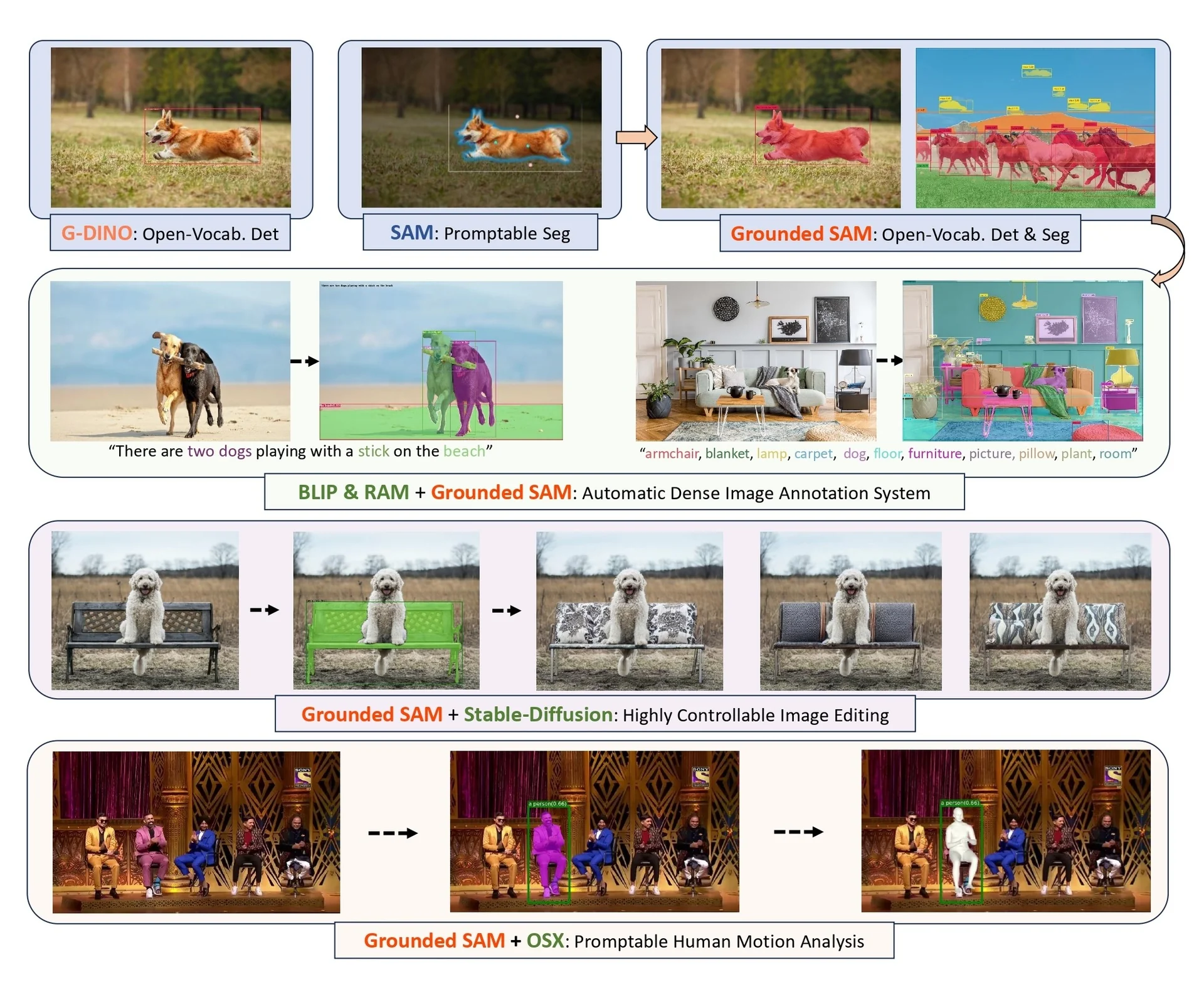
Motivation and context
From closed-set segmentation to open-world understanding Classical segmentation backbones such as Mask R-CNN or Mask2Former learn on fixed label sets (for example, the 80 COCO categories) and cannot directly handle unseen concepts.
Mask DINO [340] improved this situation by unifying detection and segmentation in a single Transformer decoder, but it still assumes a closed vocabulary tied to the training datasets. Extending such architectures to genuinely open-vocabulary segmentation requires either retraining on large-scale vision–language corpora or adding a separate recognition head.
In parallel, foundation segmentation models such as SAM [309] and SAM 2 [529] took a different path. They abandon fixed labels altogether, and instead learn a powerful promptable segmentation model trained on billions of masks (SA-1B). Given an image and spatial prompts (points, bounding boxes, or coarse masks), SAM returns high-quality instance masks even for rare or never-before-seen categories. However, SAM and SAM 2 do not know which object to segment from text; they require the user to specify prompts in image coordinates.
Open-vocabulary detectors such as Grounding DINO [384] fill the complementary gap. Grounding DINO extends DETR-style detection to arbitrary phrases by aligning region features with text embeddings, returning boxes and phrase matches for arbitrary natural language queries. Yet Grounding DINO only produces bounding boxes; it does not output segmentation masks and thus cannot be used directly for fine-grained per-pixel tasks.
Grounded SAM is motivated precisely by these complementary strengths and weaknesses. It asks: Instead of training another huge model, can one assemble existing open-world detectors and promptable segmenters into a single pipeline that supports open-vocabulary detection, segmentation, and more complex tasks?
Model assembly as an alternative to unified training The introduction of Ren et al. [540] contrasts three families of approaches for open-world vision tasks.
- Unified models. Large, multi-task models such as UNINEXT or OFA are trained end-to-end on a mixture of datasets to support multiple tasks in one network. They are conceptually elegant, but require huge training compute, large curated datasets, and are difficult to maintain or extend once deployed. Moreover, performance on specialized tasks like open-set segmentation is often limited by compromises inherent in joint training.
- LLM-as-controller pipelines. Recent systems such as HuggingGPT and Visual ChatGPT treat vision models as callable tools under the control of a large language model. These systems are flexible and user-friendly, but remain bottlenecked by the availability and quality of specialized vision tools for core tasks like segmentation.
- Ensemble foundation models (Grounded SAM). Grounded SAM chooses a middle ground: instead of training a new foundation model or delegating everything to an LLM, it assembles existing open-world models into a modular pipeline. Open-vocabulary detection is delegated to Grounding DINO, pixel-accurate segmentation to SAM or SAM 2, tagging to RAM, captioning to BLIP, generation to Stable Diffusion, and 3D pose/mesh recovery to OSX. This decomposition retains the strengths of each expert while enabling new compound tasks like automatic open-vocabulary dense annotation and prompt-based human motion analysis.
The next parts describe the core detection–segmentation pipeline, then detail how Grounded SAM composes additional experts around this core.
Core pipeline: from text prompts to segmentation masks
Grounded SAM’s central component is an open-vocabulary detection–and–segmentation pipeline that takes an image and natural language prompt as input and outputs bounding boxes, category phrases, and corresponding masks.
Conceptually, it decomposes open-set segmentation into two steps:
- 1.
- Use Grounding DINO to perform open-set detection and obtain bounding boxes associated with text phrases and confidence scores.
- 2.
- Use SAM (or SAM 2 / HQ-SAM variants) to perform promptable segmentation conditioned on those boxes.
While the paper is largely qualitative and does not introduce new losses or training objectives, it is useful to formalize this pipeline.
Notation and problem setup Let \(I \in \mathbb {R}^{H \times W \times 3}\) denote an RGB image and \(T\) a text prompt that may contain one or multiple phrases describing desired targets, for example \[ T = \mbox{``Butterfly, bag, shoes, hair, white T-shirt.''}. \] Grounding DINO tokenizes \(T\) into phrases \(\{p_k\}_{k=1}^K\) and produces text embeddings \(\mathbf {t}_k\). Given \((I,T)\), the detector predicts a set of \(N\) candidate regions \[ \mathcal {R} = \{(b_i, s_i, q_i)\}_{i=1}^{N}, \] where \(b_i\) is a bounding box in image coordinates, \(s_i\) is a scalar confidence score, and \(q_i \in \{1,\dots ,K\}\) is the index of the matched text phrase for that box. Boxes and phrase matches are obtained by a DETR-style decoder with cross-attention between visual and textual tokens, as detailed in the Grounding DINO enrichment.
SAM receives the image \(I\) and a set of spatial prompts \(\{b_i\}\) and returns a collection of binary masks \(\{M_i\}\) and quality scores \(\{\hat {s}_i\}\), where each \(M_i \in \{0,1\}^{H \times W}\) is a segmentation mask corresponding approximately to \(b_i\). Grounded SAM associates each mask \(M_i\) with the phrase \(p_{q_i}\) and the combined score \(s_i\) (possibly fused with \(\hat {s}_i\)).
Formally, the pipeline implements a mapping \[ (I, T) \longmapsto \{(p_{q_i}, b_i, M_i, s_i)\}_{i=1}^{N'}, \] where \(N'\) is the number of detections remaining after thresholding and non-maximum suppression (NMS).
Step 1: open-vocabulary detection with Grounding DINO Grounding DINO [384] encodes the image with a Vision Transformer and the text prompt with a BERT-style text encoder. Through a multi-stage feature enhancer and cross-modality decoder, it produces region features aligned with text tokens and predicts:
- Bounding boxes \(\{b_i\}_{i=1}^{N}\) in \((x_{\min }, y_{\min }, x_{\max }, y_{\max })\) coordinates.
- Per-box matching scores over phrases, often realized as dot products between region features and text embeddings, followed by a sigmoid.
Grounded SAM uses the official Grounding DINO implementations for both Base and Large backbones. Given detection outputs, it applies configurable thresholds:
- A box threshold \(\tau _{\mbox{box}}\) serves as a primary confidence filter, keeping only regions whose maximal alignment score with the prompt exceeds a preset value.
- A text threshold \(\tau _{\mbox{text}}\) further filters the phrase associations for each surviving box, ensuring that the predicted phrase is strongly aligned with the corresponding region.
Boxes failing either threshold are discarded, and the remaining boxes undergo standard NMS. The result is a set of high-confidence, text-labeled boxes \(\{(b_i, p_{q_i}, s_i)\}_{i=1}^{N'}\).
Step 2: promptable segmentation with SAM SAM [309] consists of a ViT image encoder, a prompt encoder, and a mask decoder. For Grounded SAM, the relevant prompt type is the bounding box prompt. For each selected box \(b_i\):
- 1.
- The image \(I\) is resized and padded to \(1024\times 1024\) resolution (SAM’s default) and passed once through the SAM image encoder to obtain an image embedding \(\mathbf {E} \in \mathbb {R}^{H' \times W' \times C}\).
- 2.
- The box \(b_i\) is transformed to the resized coordinate frame and encoded by SAM’s prompt encoder into a low-dimensional embedding \(\mathbf {p}_i\).
- 3.
- The mask decoder attends to \(\mathbf {E}\) conditioned on \(\mathbf {p}_i\), producing several candidate masks \(\tilde {M}_i^{(k)}\) and corresponding mask quality scores \(\hat {s}_i^{(k)}\).
In the official pipeline, only the highest-quality mask per box is retained: \[ M_i = \tilde {M}_i^{(k^\star )}, \quad k^\star = \arg \max _k \hat {s}_i^{(k)}. \] The combined confidence for the instance can be taken as \(s_i\) (from Grounding DINO), \(\hat {s}_i^{(k^\star )}\) (from SAM), or a product of both; the public code uses a simple combination that preserves the detector’s ranking.
Step 3: merging detections and masks Once masks are predicted for all boxes, Grounded SAM performs light-weight post-processing:
- Masks with extremely small area or low combined confidence are suppressed.
- Overlapping masks can be resolved by favoring higher-scoring instances, optionally in a class-wise manner (that is, by phrase).
- The final output is a set of instance masks \(M_i\) with their associated phrases \(p_{q_i}\) and boxes \(b_i\), effectively yielding open-vocabulary instance segmentation.
The following figure illustrates the resulting behavior: arbitrary phrases, including long-tail species names, can be grounded to both boxes and masks.
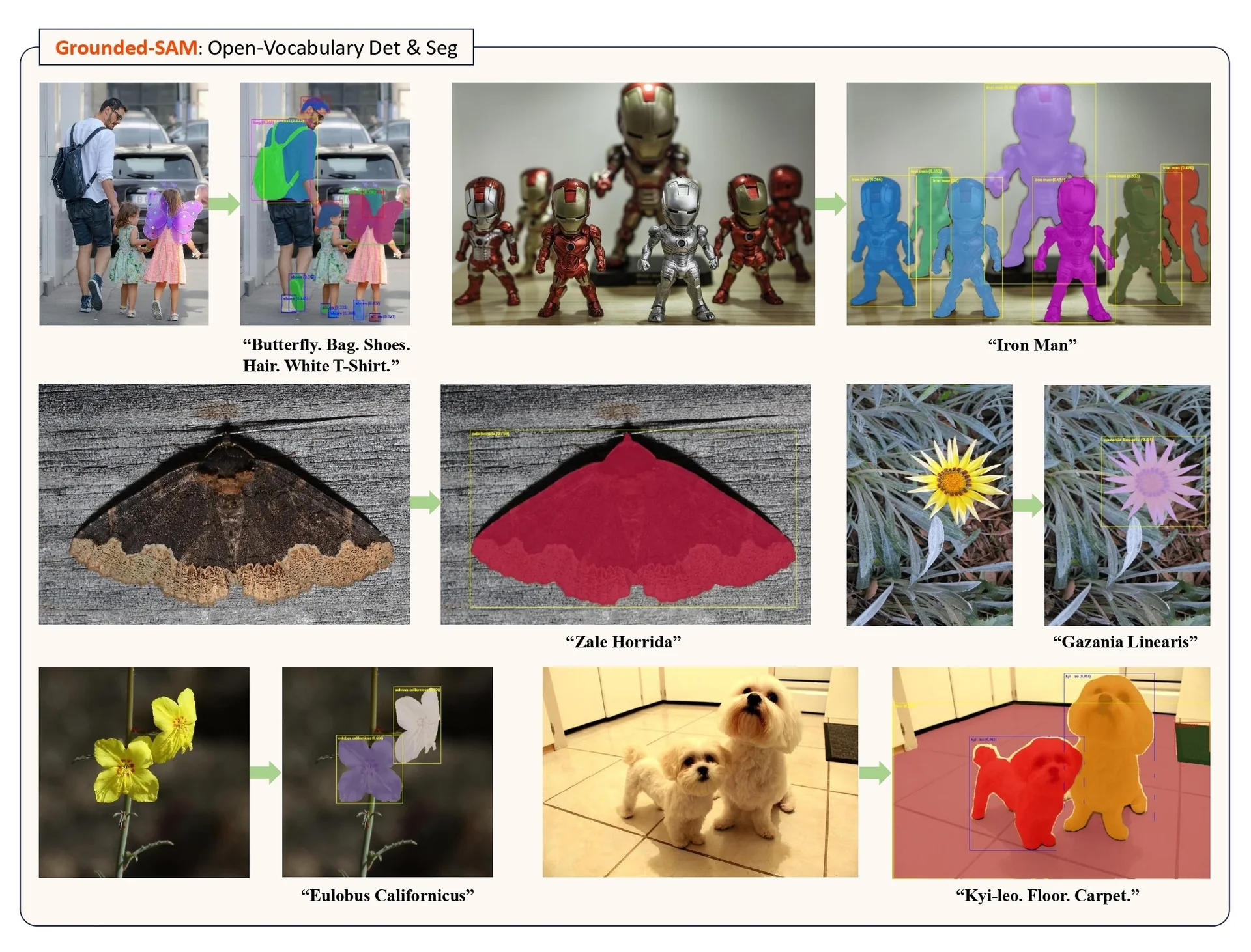
Pseudo-code for the core pipeline The open-vocabulary detection–and–segmentation pipeline implemented in the official repositories can be summarized as follows.
def grounded_sam(image,       text_prompt,
                 box_threshold=0.25,
                 text_threshold=0.25,
                 nms_iou_threshold=0.5):

"""
Core Grounded SAM pipeline:
open-vocabulary detection (Grounding DINO)
+ promptable segmentation (SAM).
"""

# 1. Open-vocabulary detection with Grounding DINO.
#    Returns boxes (xyxy in image coords), phrase ids,
#    and detection scores.
boxes, phrase_ids, det_scores = grounding_dino(
    image=image,
    text=text_prompt
)

# 2. Thresholding and non-maximum suppression.
keep = []
for i, (b, pid, score) in enumerate(zip(boxes,
                                        phrase_ids,
                                        det_scores)):
    if score < box_threshold:
        continue
    if phrase_score(pid) < text_threshold:
        continue
    keep.append(i)
boxes = boxes[keep]
phrase_ids = phrase_ids[keep]
det_scores = det_scores[keep]
boxes, phrase_ids, det_scores = nms(
    boxes, phrase_ids, det_scores,
    iou_thresh=nms_iou_threshold
)

# 3. Single SAM image embedding.
sam_image = preprocess_for_sam(image)  # resize+pad to 1024x1024
image_features = sam_image_encoder(sam_image)

# 4. For each box, run SAM mask decoder.
masks, mask_scores, phrases = [], [], []
for b, pid, score in zip(boxes, phrase_ids, det_scores):
    box_prompt = encode_box_prompt(b, image_shape=image.shape)
    candidate_masks, candidate_scores = sam_mask_decoder(
        image_features, box_prompt
    )
    # Keep highest-scoring mask for this box.
    best_idx = candidate_scores.argmax()
    masks.append(candidate_masks[best_idx])
    mask_scores.append(candidate_scores[best_idx])
    phrases.append(id_to_phrase(pid))

return boxes, masks, phrases, det_scores, mask_scores
Assembling open-world models around Grounded SAM
Beyond open-vocabulary instance segmentation, Grounded SAM serves as a hub connecting multiple foundation models. The paper and code highlight three particularly impactful compositions, all illustrated in Figure 15.54.
Automatic dense image annotation with BLIP and RAM For building large-scale detection/segmentation datasets, manual annotation is expensive. Grounded SAM integrates:
- RAM [802], a strong image tagging model trained on large-scale image–text pairs, capable of predicting thousands of semantic tags per image.
- BLIP [344], a vision–language model for captioning and image–text understanding.
Two complementary pipelines are described.
- Tag-driven annotation (RAM + Grounded SAM). RAM predicts a list of tags \(\{t_k\}\) for an image. These tags are assembled into one or more text prompts \(T\) (in practice, long tag lists are often split into several batches to respect the text encoder’s context length and avoid attention dilution) and fed to Grounded SAM, which produces boxes and masks for each tag, yielding dense, open-vocabulary instance annotations without any manual supervision.
- Caption-driven annotation (BLIP + Grounded SAM). BLIP generates a caption describing the scene. An LLM or simple noun-phrase extractor can convert this caption into a list of object phrases, again fed into Grounded SAM as the text prompt. This variant is especially useful in settings where human-like descriptions are more natural than category lists.
From a systems perspective, Grounded SAM supplies spatial grounding (where objects are), while RAM and BLIP supply semantic coverage (what they are). This composition is explicitly positioned as a practical recipe for building diverse segmentation datasets without manual labeling.
Controllable image editing with Stable Diffusion Grounded SAM also acts as a front-end for region-aware image editing with latent diffusion models such as Stable Diffusion [548]. The high-level pipeline is:
- 1.
- Use Grounded SAM with a text prompt like “bench” to obtain a mask \(M\) for the target object.
- 2.
- Convert \(M\) into an inpainting mask (typically a binary map where \(1\) marks pixels to be resynthesized) and pass \((I, M)\), together with a new text prompt (for example, “a bench with floral upholstery”), to Stable Diffusion’s inpainting model.
- 3.
- The diffusion model resynthesizes only the masked region while preserving the unmasked pixels of the original scene.
Figure 15.54 (third row) demonstrates editing a dog’s bench into different textures while maintaining consistent background and dog appearance. The key insight is that, for controllable editing, precise region masks are more valuable than global CLIP-style text–image alignment; Grounded SAM provides exactly such masks given natural language descriptions.
Promptable human motion analysis with OSX Finally, Grounded SAM integrates with OSX [364], a one-stage 3D whole-body mesh recovery model that predicts SMPL-X parameters from images. Typically, OSX operates on person crops localized by an off-the-shelf detector. Grounded SAM replaces this detector with text-driven grounding:
- 1.
- A user query such as “the person in white clothes” is passed, together with the input frame, into Grounded SAM, obtaining a mask and bounding box for the target person.
- 2.
- The RGB crop defined by this bounding box is fed into OSX, which estimates 3D body, hand, and face meshes (background context inside the crop is retained, since it helps resolve pose and camera ambiguity).
- 3.
- Downstream analytics or visualization tools operate on the reconstructed 3D motion.
This composition realizes promptable motion analysis: text specifies which subject to track, Grounded SAM localizes and segments that subject across frames (often using SAM 2 for video), and OSX reconstructs the 3D motion.
Architecture and implementation details
Although Grounded SAM introduces no new neural architectures, implementation choices significantly affect usability and performance.
Backbones and model variants The paper and code support several detector–segmenter combinations.
- Grounding DINO variants. Experiments primarily use Grounding DINO-Base and Grounding DINO-Large backbones, which differ in depth and width of the visual backbone (often Swin transformers) and the text encoder configuration.
- Segmentation backbones. For segmentation, SAM-H (ViT-H backbone) is the default, but the public demos also support SAM-B and SAM-L, HQ-SAM (a high-quality mask-refinement variant of SAM), and efficient SAM versions for faster inference.
- Grounded HQ-SAM. “Grounded HQ-SAM” [297] denotes the configuration combining Grounding DINO-Base with HQ-SAM-H, used in some experiments to probe the effect of segmentation quality.
Preprocessing and coordinate handling Coordinate consistency between Grounding DINO and SAM is crucial.
- The input image is read at its original resolution, and Grounding DINO’s preprocessing stack (typically resizing the shorter side and normalizing) is applied before detection.
- Detected bounding boxes are output either in the resized image frame or in normalized \([0,1]\) coordinates; they must first be projected back to absolute coordinates on the original image.
- Before segmentation, the original image is resized and padded to SAM’s square input size (for example, \(1024\times 1024\)), and the boxes are then rescaled and shifted into this coordinate system, preserving the spatial correspondence between boxes and content.
The official repositories hide these details behind helper functions, but for reproducibility in research code it is important to respect this two-stage rescaling.
Thresholds and hyperparameters Default hyperparameters in the demo scripts include:
- Box threshold \(\tau _{\mbox{box}}\) in the range \([0.25, 0.5]\), controlling detector confidence.
- Text threshold \(\tau _{\mbox{text}}\) typically around \(0.2\)–\(0.25\), filtering weak phrase–region alignments.
- NMS IoU threshold around \(0.5\).
- Maximum number of detections per image, often \(N' \leq 100\), to keep segmentation overhead manageable.
In practice, users adjust these according to their application: lower thresholds for recall-oriented data annotation, higher thresholds for interactive editing.
SAM vs. SAM 2 The original paper [540] and the initial repositories focus on image-level SAM, but subsequent extensions (Grounded-SAM-2) integrate SAM 2 [529]. In this configuration:
- Grounding DINO is typically run only on key frames to obtain initial boxes.
- SAM 2’s streaming memory tracks and updates masks across subsequent frames, using the initial boxes and masks as prompts.
This design preserves the text grounding benefits of Grounding DINO while exploiting SAM 2’s efficient video mask propagation.
Experiments and analysis
SegInW zero-shot benchmark The primary quantitative evaluation in the paper is on SegInW (Segmentation in the Wild), a challenging zero-shot benchmark that unifies 25 segmentation datasets covering diverse domains and label spaces. SegInW reports mean average precision (mAP) across datasets without any training on SegInW itself.
Grounded SAM is evaluated as a plug-in on top of Grounding DINO and SAM variants, and compared to strong open-world segmentation baselines including X-Decoder, ODISE, OpenSeeD, SAN-CLIP, and UNINEXT. The summary results reported in Ren et al. [540] are:
- A configuration with Grounding DINO-Base and SAM-H (denoted “Grounded-SAM (B+H)”) achieves 48.7 mean AP, substantially outperforming unified segmentation models such as OpenSeeD-L (36.7 mean AP) and UNINEXT-H (42.1 mean AP), and also improving over SAN-CLIP-ViT-L (41.4 mean AP).
- Replacing SAM-H with HQ-SAM-H (“Grounded-HQ-SAM (B+H)”) further improves mean AP to 49.6, highlighting that segmentation quality can be a limiting factor once detection and text grounding are strong.
These numbers underscore a central message of Grounded SAM: composing specialized open-world detectors and segmenters can outperform complex unified models, even without joint training.
Qualitative analysis on long-tail categories Beyond SegInW, the paper presents numerous qualitative examples, some of which are shown in Figure 15.55. A notable aspect is robustness to long-tail and fine-grained categories, for example:
- Botanical and entomological species such as “Gazania linearis” and “Zale horrida”.
- Compositional or attribute-rich phrases such as “white T-shirt”, “yellow flower”, or “Iron Man” (referring to a toy figure).
Because Grounding DINO is trained on large-scale grounding datasets and benefits from CLIP-like text–image alignment, it can localize such phrases even when segmentation datasets do not contain corresponding labels. SAM then refines localization to pixel-level masks, yielding high-quality visualizations.
Effect of segmentation backbones Although the paper does not present extensive ablation tables, comparisons across segmentation backbones (SAM vs. HQ-SAM) effectively act as an ablation on the segmentation component.
- Grounded-HQ-SAM consistently improves or matches Grounded-SAM on SegInW, especially on datasets where boundary precision is critical.
- This suggests that, once text grounding and detection are sufficiently strong, downstream performance is largely bottlenecked by mask quality, and improvements in SAM-like models translate directly into better open-world segmentation.
This observation is important for downstream practitioners: upgrading the segmentation backbone can yield measurable gains without modifying the detection or training pipeline.
Limitations and the case for a unified model
Grounded SAM is intentionally a systems paper, focusing on model assembly rather than new architectures. This makes it an excellent practical recipe, but it also exposes structural bottlenecks that become increasingly problematic as one pushes toward real-time, large-scale, open-set segmentation. These bottlenecks point directly toward the need for a unified foundation model such as SAM 3, which will be introduced next.
Redundant encoders and runtime cost A central limitation of Grounded SAM is computational redundancy. Because the detector (Grounding DINO) and the segmenter (SAM or SAM 2) are distinct models with separate weights, the image must be processed multiple times.
- Double encoding. The pipeline typically runs a large visual backbone for Grounding DINO (for example, a Swin-L or ViT-based encoder) to produce open-vocabulary box proposals, and then runs a second heavy backbone in SAM (for example, ViT-H) to produce mask features. Even though both stages extract high-level visual features, there is no shared computation between them, roughly doubling latency and memory usage compared to a single-encoder design.
- Scaling to large images and video. For high-resolution images or video streams, this double encoding becomes especially expensive: every frame must be encoded by the detector and then again by the segmenter. Even with SAM 2’s efficient memory mechanism, the need to invoke a separate open-vocabulary detector on key frames remains a significant runtime and deployment cost.
For applications that need interactive performance, deployment on edge devices, or long video sequences, this two-stage architecture is therefore a poor match. A natural next step is to design a single shared encoder whose features serve both open-vocabulary localization and pixel-level segmentation, as pursued by SAM 3.
Boxes as a lossy interface between text and masks Grounded SAM passes information between the text-conditioned detector and the segmenter only through bounding boxes. This design is simple and modular, but it introduces an information bottleneck that limits both accuracy and the expressiveness of open-set segmentation.
- Heuristic coupling and thresholds. The interface between models is governed by hand-tuned thresholds such as the box score threshold \(\tau _{\mbox{box}}\) and text score threshold \(\tau _{\mbox{text}}\), plus non-maximum suppression. These hyperparameters control which detections are forwarded to SAM, but they are not learned jointly with the segmentation objective, and there is no gradient flow from masks back to text embeddings or detector features.
- Imperfect proxies for shape. Bounding boxes are a coarse, axis-aligned approximation to object extent. For thin, elongated, occluded, or overlapping objects, boxes may cover large background regions or multiple instances. SAM is then asked to infer the intended mask from a noisy, sometimes ambiguous box prompt that was not optimized for SAM’s training distribution, leading to suboptimal boundaries or missed instances.
From the perspective of open-set segmentation, this means that text grounding and mask prediction live in separate spaces: text directly influences box proposals, but not the mask decoder. A unified model such as SAM 3 is motivated to let text tokens interact directly with segmentation tokens, avoiding boxes as the sole communication channel.
Limited learning of open-set segmentation behavior Because Grounded SAM assembles pre-trained components without end-to-end optimization, its ability to learn better open-set segmentation behavior is constrained.
- Frozen experts and no joint training. Grounding DINO, SAM, RAM, and BLIP are typically used in frozen form. Errors from later stages (such as poor masks) cannot drive improvements in the detector or text encoder, and dataset-specific supervision cannot be used to jointly refine all modules in a coherent way.
- Open-vocabulary only in detection. Open-vocabulary capability resides almost entirely in Grounding DINO’s text–box matching. SAM’s segmentation head remains class-agnostic and is never explicitly aligned with text embeddings. As a result, the system behaves as an open-vocabulary detector followed by a generic segmenter, rather than a genuinely text-aware open-set segmentation model.
A unified architecture can instead learn a single multi-modal representation in which detection queries, segmentation tokens, and text embeddings are trained together, closing this gap.
Toward SAM 3: fusing detection, text, and segmentation In summary, Grounded SAM demonstrates that carefully assembling existing open-world detectors, segmenters, taggers, captioners, generative models, and 3D estimators can yield powerful open-vocabulary workflows without retraining gigantic unified models. At the same time, its double-encoder design, reliance on bounding boxes as a lossy interface, and lack of joint optimization limit both runtime efficiency and the quality of open-set segmentation, especially at scale.
These observations motivate the next step in this sequence of enrichments: SAM 3, covered in the next subsection. Rather than gluing together a detector and a segmenter, SAM 3 is designed as a single foundation architecture that unifies text grounding, region localization, and pixel-precise segmentation within one end-to-end trainable model, addressing many of the structural limitations highlighted above.
Enrichment 15.7.5: SAM 3: Segment Anything with Concepts
Motivation: from visual prompts to concepts
From promptable visual segmentation to concept-level segmentation The original Segment Anything Model (SAM) [309] introduced promptable visual segmentation (PVS): given an image and a visual prompt (points, boxes, or masks), the model returns a high-quality mask for the object indicated by that prompt. SAM 2 [529] extended this idea to video, adding a memory-based tracker that propagates masks across frames while still relying on geometric prompts to specify which object to follow. In both cases, prompts are spatial and instance-specific: the user must explicitly enumerate the targets by providing a separate local prompt for each object of interest, and the model only segments objects that have been individually prompted, remaining agnostic to their semantic categories.
Mask DINO [340] and other DETR-style models unified detection and segmentation under a fixed label vocabulary, but remained fundamentally closed-set: they predict over a pre-defined list of categories. Grounded SAM [540] partially broke this limitation by composing an open-vocabulary detector (Grounding DINO [384]) with SAM or SAM 2. Text prompts such as “a red car” are first converted to bounding boxes, which are then handed to SAM for mask prediction. This composite design enables open-vocabulary segmentation but keeps recognition (text-to-box) and segmentation (box-to-mask) as separate systems, with no single model deciding both whether a concept is present and how it should be segmented. It also inherits several practical drawbacks: two large models are executed sequentially (detector then segmentor), increasing latency and memory footprint; there is no joint optimization of box prediction and mask quality, so errors in the detector (e.g., missed or mis-localized boxes, confidence miscalibration) propagate directly into the segmentation stage; and the detector is trained to produce boxes that are optimal for detection metrics rather than for downstream mask refinement.
SAM 3 [65] is designed to close this gap by changing the underlying objective. It introduces Promptable Concept Segmentation (PCS), where the input is a concept prompt and the default output is all instances of that concept, segmented and (for video) tracked with persistent identities. Unlike PVS—which assumes a user has already selected a specific instance to segment and requires explicit spatial enumeration of each target—PCS must first decide whether the concept is present anywhere in the media and then discover and localize every matching instance from a single semantic command. Crucially, this is done within a single model that jointly learns recognition and segmentation: the same Perception Encoder backbone and DETR-style decoder are optimized end-to-end for concept presence, localization, and mask quality, avoiding the error compounding and objective mismatch of separated detector+segmentor pipelines. In practice, this does not preclude single-object workflows: users can either fall back to PVS-style visual prompts (points, boxes) or run PCS once and then select a single predicted instance to refine and track as needed. Concept prompts are defined as either:
- Short noun phrases. Simple text such as “striped cat”, “round cell”, or “hard hat”, restricted to a noun plus optional modifiers.
- Image exemplars. One or more bounding boxes on example instances, each marked as positive or negative.
- Text–image combinations. A noun phrase plus positive and negative exemplars to refine or disambiguate the concept.
In PCS, the model must decide both whether the concept is present at all and, if so, which pixels and object instances match the prompt across the entire image or video.
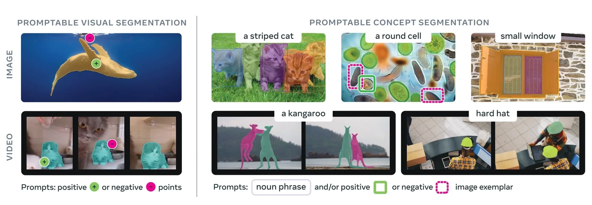
The comparison in Figure 15.56 highlights two regimes.
- Promptable Visual Segmentation (PVS). A user clicks on a particular object (e.g., a cat or a whale), and the model returns a mask for that specific instance, which SAM 2 can then track across a video; additional instances require additional, explicitly enumerated prompts.
- Promptable Concept Segmentation (PCS). A user issues a concept prompt like “a striped cat” or “a round cell”. SAM 3 segments all instances matching that concept in an image or video, and assigns consistent instance IDs over time. In a downstream single-object setting, one of these instances can then be selected and treated as the target of interest.
Ambiguity and the need for new data and metrics Open-vocabulary PCS is inherently ambiguous. Simple noun phrases can be:
- Polysemous. Phrases like “mouse” may refer to an animal or a computer device depending on context.
- Subjective or vague. Adjectives such as “cozy” or “large” depend on human judgment.
- Boundary-ambiguous. Concepts like “mirror” may or may not include the frame; “toilet roll holder” may or may not include the roll itself.
- Occluded or blurred. Partial visibility complicates deciding whether an instance should be included and where its boundaries lie.
Standard closed-vocabulary benchmarks deliberately avoid much of this messiness. Closed-vocabulary datasets (e.g., LVIS) mitigate these issues by carefully curating class definitions and mask guidelines. In contrast, SAM 3 targets any simple noun phrase that can be grounded visually, which requires:
- A large, diverse dataset. With millions of unique noun phrases and high-quality instance masks across images and videos.
- Evaluation protocols. That admit multiple valid interpretations of the same phrase.
- Model components. Specifically designed to decouple recognition (“is this phrase present?”) from localization (“where are its instances?”) and to handle ambiguous cases.
To this end, SAM 3 introduces a large-scale Segment Anything with Concepts (SA-Co) dataset and a classification-gated F1 metric (cgF1) tailored for PCS, discussed below in the Experiments part. The following figure previews qualitative improvements over a strong open-vocabulary baseline.
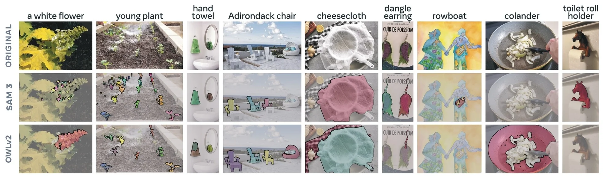
Method: promptable concept segmentation
Task inputs and outputs Formally, SAM 3 solves the PCS task defined in Section 2 of the paper [65]: given a concept prompt and a piece of visual media, it must decide whether the concept is present and, if so, detect, segment, and (for videos) track all matching instances.
Inputs.
- Media. A single RGB image or a short video clip.
-
Concept prompt. A global description of the target concept, applied to the entire image or video. It can take any of the following forms:
- Text-only. A simple noun phrase (NP), such as “striped cat”, “round cell”, or “hard hat”.
- Exemplar-only. One or more image exemplars, given as bounding boxes labeled positive or negative, defining the concept purely in visual terms.
- Text + exemplars. A noun phrase combined with positive/negative exemplars to refine or disambiguate the concept.
Unlike PVS prompts, which are tied to a specific instance (a particular click or box), PCS prompts define the concept and ask the model to find all instances that match it.
Outputs.
- Instance-level outputs. A set of object hypotheses for the concept, each with a bounding box, an instance mask, and a confidence score (used for cgF1 evaluation and downstream selection).
- Semantic output. A binary segmentation map indicating, for each pixel, whether it belongs to any instance of the prompted concept (obtained by aggregating instance masks).
- Video tracks. For videos, a collection of spatio-temporal masklets: sequences of masks with persistent identities across frames, representing how each instance of the concept moves and evolves over time.
Architecture and implementation details
High-level data flow from prompts to outputs The previous paragraphs defined PCS at the interface level: given a media input (image or short video) and a concept prompt, SAM 3 returns instance-level hypotheses, semantic masks, and (for video) temporally consistent masklets. Internally, these outputs are produced by a tightly coupled but modular architecture:
- Perception Encoder (PE). A shared vision backbone that extracts a multi-scale feature pyramid for each frame.
- Prompt-conditioned DETR-style detector. Consumes PE features and prompt tokens (text and exemplars) to predict concept-specific queries, boxes, and masks.
- Global presence head. Decides whether the concept exists anywhere in the input and gates the local query scores.
- SAM 2-style tracker. Propagates masklets over time using PE features and a memory bank, periodically re-anchored by the detector.
- Training pipeline and data engine. Jointly shape the PE, detector, and tracker, and provide large-scale SA-Co supervision tailored to PCS.
At inference time for an image:
- PE. Produces a multi-scale feature pyramid from the input image.
- Prompt encoders. Turn the concept prompt (text and optional exemplars) into a sequence of tokens.
- Detector. A fusion encoder and DETR-style decoder output query-wise scores, boxes, and masks.
- Presence head. Gates these scores to yield calibrated instance-level and semantic predictions.
For videos, the same detector runs per frame while the tracker maintains and updates masklets using a memory bank and periodic re-prompting from the detector.
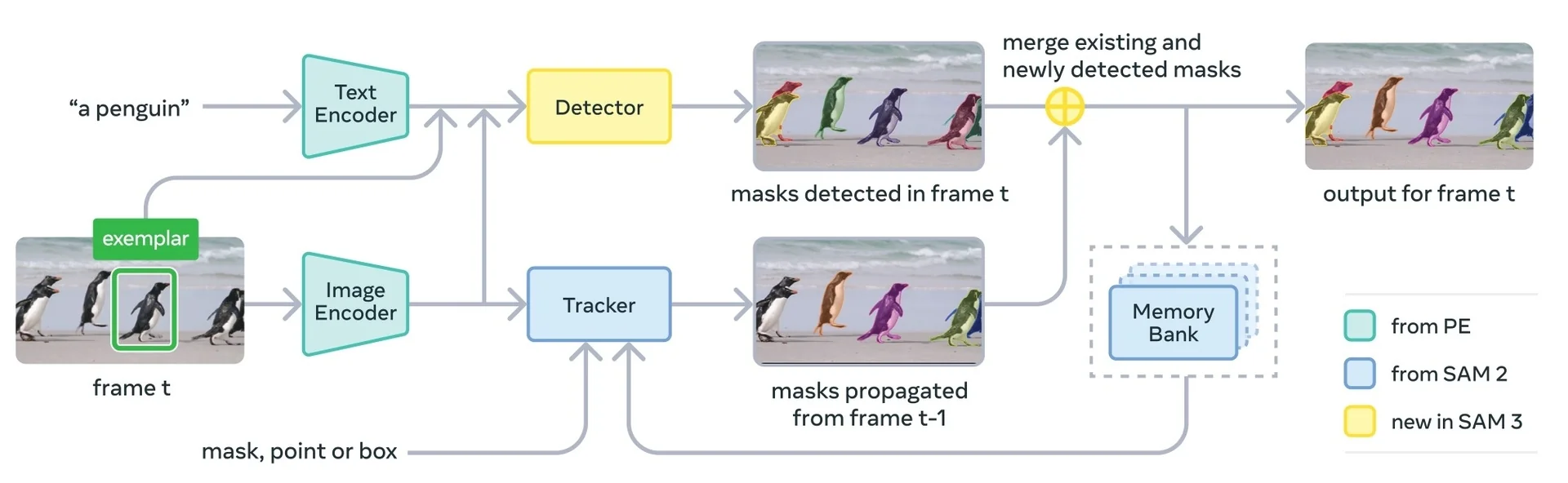
The next paragraphs first detail the Perception Encoder backbone that powers the system, then describe how its features are consumed by the Detector, Presence head, and Tracker, and finally summarize the Training stages and Data pipeline that make this unified PCS design effective.
The Perception Encoder (PE)
Motivation: beyond CLIP for dense prediction Standard contrastive vision–language models such as CLIP [512] excel at zero-shot image-level classification and retrieval, but they are poorly suited to dense prediction tasks. The CLIP objective compresses an entire image into a single global vector, and the network is explicitly trained to discard spatial detail that is not needed to decide which caption matches the image. This is ideal for global recognition, but problematic for tasks like segmentation and tracking that require precise boundaries and temporally stable spatial structure.
Conversely, dense models such as SAM 2 [529] are optimized for geometry, not semantics; they produce excellent masks given geometric prompts, but they do not natively understand open-vocabulary text. Grounding-style models partially bridge this gap by pairing a CLIP-like encoder with a detector, but they still treat global semantics and dense geometry as largely separate modules.
The Perception Encoder (PE) [48] is designed as a “better CLIP” that is directly usable for dense and video tasks. It provides a single large vision trunk whose representations are:
- Semantically expressive. Capable of interpreting open-vocabulary text prompts via contrastive vision–language pretraining.
- Spatially precise. Preserving pixel-level geometry and object boundaries required for mask decoding.
- Temporally stable. Robust under frame-to-frame variations, which is essential for tracking.
This combination is particularly attractive for SAM 3: instead of gluing together a CLIP-like semantic encoder and a separate dense backbone, SAM 3 can share one alignment-tuned visual encoder across concept detection, segmentation, and tracking.
Two-stage design: PE Core and alignment-tuned variants Conceptually, PE provides a single high-capacity visual trunk that is trained once and then adapted to two usage regimes:
- PE Core: a contrastively trained vision backbone used as the starting point.
- Alignment-tuned variants: PE Language for multimodal language modeling and PE Spatial for dense prediction and tracking.
PE follows a two-stage training process:
- 1.
- Stage 1: Contrastive vision–language pretraining (PE Core). Starting from an OpenCLIP ViT-L/14 baseline, PE Core is trained on large-scale image and video data with a CLIP-style contrastive objective. For each image \(x\) and paired text \(y\), a vision encoder \(f_{\theta }\) and a text encoder \(g_{\phi }\) produce global embeddings, and a temperature-scaled InfoNCE loss encourages matched pairs to have high cosine similarity and mismatched pairs to be far apart. Video clips are treated as additional views with temporal augmentations and shared captions.
- 2.
- Stage 2: Alignment tuning from intermediate layers. After
contrastive pretraining, PE Core’s intermediate layers are probed.
Lightweight heads are then trained on top of frozen (or lightly tuned)
intermediate features to specialize the encoder for:
- Language alignment (PE Language). Features are projected into a multimodal LM token space so that downstream LMs can “read” them as visual tokens (e.g., for OCR, captioning, VQA).
- Spatial alignment (PE Spatial). Features are aligned to dense prediction teachers (including SAM 2.1) so that final-layer tokens remain geometrically precise while retaining strong semantics.
The following figure summarizes this framework: the left block shows contrastive pretraining; the middle illustrates frozen-feature extraction from intermediate layers; and the right side shows the two specialized heads, PE Language and PE Spatial.
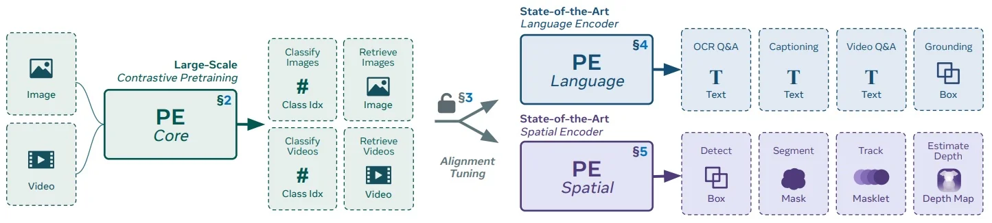
Promptable Concept Segmentation (PCS) places three simultaneous demands on the visual backbone:
- Semantically expressive. The model must interpret short noun phrases and relate them to visual content.
- Spatially precise. The model must preserve fine-grained geometry to decode masks and boundaries.
- Temporally stable. The model must support tracking of masklets across video sequences without drift.
PE’s two-stage design and dual alignment pathways are specifically constructed to meet these requirements, enabling SAM 3 to unify open-vocabulary reasoning, dense segmentation, and robust tracking.
Stage 1: PE Core — contrastive pretraining and robust features PE Core uses a CLIP-style contrastive objective but with a heavily refined training recipe aimed at robustness and transfer, rather than just ImageNet accuracy. At a high level, PE Core encodes an input image \(x\) into a grid of patch tokens \[ z = f_{\theta }(x) \in \mathbb {R}^{H'W' \times D}, \] and an attention-pooling block produces a global embedding \(h(x) \in \mathbb {R}^D\) from these tokens. Paired text \(y\) is encoded by a separate text tower into \(t(y) \in \mathbb {R}^D\), and a symmetric contrastive loss is applied over \((h(x), t(y))\) across the batch. For video, temporal crops, frame sampling, and shared captions are used to create additional positive pairs.
The evolution of the PE Core recipe is shown in the following figure.
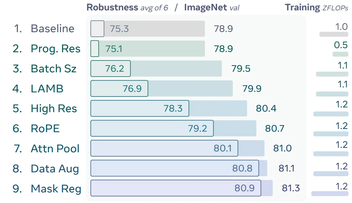
The main modifications, and how they are implemented, are:
- Progressive resolution. Training begins at low resolution (e.g., \(128\times 128\)) and progressively increases to high resolution (e.g., \(448\times 448\)). Early in training, smaller images reduce FLOPs and stabilize optimization; later, higher resolutions restore fine detail, improving downstream dense prediction without requiring a full high-resolution schedule from scratch.
- Large-batch optimization with LAMB. Contrastive learning benefits from very large batch sizes (tens of thousands of examples) to provide many hard negatives. However, standard optimizers such as AdamW struggle at this scale. PE therefore uses LAMB (Layer-wise Adaptive Moments optimizer for Batch training), which computes for each layer \(l\) a trust ratio \[ r_l = \frac {\|w_l\|_2}{\|\hat {g}_l\|_2 + \epsilon }, \] where \(w_l\) are the weights and \(\hat {g}_l\) is the Adam-style preconditioned gradient. The actual update is then scaled by \(r_l\), so layers with small weights and large gradients receive smaller effective steps and vice versa. This layer-wise normalization lets the optimizer safely scale to very large batch sizes without divergence, improving the quality of the contrastive negatives.
- 2D RoPE positional embeddings. Instead of learned absolute positional embeddings tied to a specific resolution, PE uses 2D Rotary Positional Embeddings (RoPE) applied to query/key vectors in attention. This encodes relative positions in a resolution-agnostic way, improving robustness to crops, rescaling, and aspect-ratio changes.
-
Attention pooling. PE replaces the standard ViT/CLIP strategy of using a single learned CLS token for global aggregation with a dedicated attention-pooling module (AttnPool) [780, 48]. This module summarizes the entire spatial feature map after the backbone has finished processing it, rather than forcing global aggregation to happen inside the backbone itself.
How global pooling normally works in ViT/CLIP. In a standard ViT, we prepend a learnable CLS token \(c_0\) to the input sequence. During each of the \(L\) transformer layers, this CLS token participates in full self-attention: \[ c_{\ell } = \mbox{SelfAttn}_{\ell }(c_{\ell -1}, Z_{\ell -1}), \quad \ell = 1,\dots ,L, \] so by the end of the network, \(c_L\) has absorbed information from every patch. However, this mechanism has two drawbacks:
- Global mixing leaks into the backbone. Since CLS attends to patches at every layer, patches also attend back to CLS. This gradually spreads global context into every patch token. Spatial tokens lose their locality and become “washed out,” which is harmful for precise mask boundaries.
- A single token must represent everything. The network is forced to compress semantics into one vector \(c_L\) through \(L\) layers of coupled attention, which makes optimizing both global semantics and local structure simultaneously difficult.
How PE’s attention pooling works and why it is different. Instead of using the CLS token as an in-network aggregator, PE treats the backbone purely as a spatial feature extractor. The ViT backbone outputs a grid of spatial tokens: \[ Z = \{z_1,\dots ,z_N\} \in \mathbb {R}^{N\times D}, \qquad N = H'W'. \] These tokens remain sharply localized because no CLS token is attending to them during backbone computation.
Only after the final backbone block, PE attaches a lightweight Transformer called the AttnPool module. It introduces a small set of “query” tokens (often just a single learnable vector \(q\)) that attends once over the frozen spatial features: \[ Q = q,\quad K = Z,\quad V = Z, \] \[ \tilde {c} = \mbox{Softmax}\!\left (\frac {QK^\top }{\sqrt {D}}\right ) V. \] Thus, \(\tilde {c}\) is a content-weighted average of all patches. Key differences from standard CLS:
- Backbone stays purely spatial. No global token is mixed inside the ViT layers, so patch tokens maintain strong locality and detailed geometry—crucial for SAM3’s mask head and tracker.
- Global aggregation happens only at the end. The global representation \(h(x)\) is computed by only one or a few AttnPool layers, not by polluting the entire backbone with global context.
- Pooling is learned, not fixed. Unlike average pooling or CLS propagation, the attention weights let the model dynamically emphasize concept-relevant regions—for example focusing on a dog’s head when the query is “striped dog”.
Finally, the pooled vector is defined as: \[ h(x) = \tilde {c}. \]
Why this is beneficial for SAM 3. SAM 3 needs a backbone that can serve two roles simultaneously:
- 1.
- Provide high-resolution, local, spatially faithful features for mask decoding and tracking.
- 2.
- Provide a global semantic embedding compatible with CLIP-style contrastive pretraining and concept presence prediction.
A CLS-through-the-backbone design forces global semantics into every patch, making spatial features less precise. AttnPool solves this tension:
- Spatial tokens stay sharp — ideal for segmentation.
- Global semantic vector \(h(x)\) is produced cleanly at the end — ideal for text–image matching and presence classification.
This late, dedicated pooling step is one of the reasons the Perception Encoder succeeds as a unified backbone for both global vision–language alignment and dense prediction, a requirement at the heart of SAM 3.
- Masked regularization. Standard CLIP training only supervises the final global embedding \(h(x)\), so the encoder can in principle rely on a few discriminative regions and ignore the rest of the image. To encourage PE Core to build coherent, spatially structured features at every location, the authors add a MaskFeat-style regularizer [710, 48]. For a small fraction of the batch (roughly \(1/16\)), they create a heavily masked view \(x_{\mbox{mask}}\) by dropping a large subset of patches. Both the original image \(x\) and the masked image \(x_{\mbox{mask}}\) are passed through the same encoder, producing token grids \[ Z_{\mbox{full}} = \{z^{\mbox{full}}_i\}_{i=1}^N, \qquad Z_{\mbox{mask}} = \{z^{\mbox{mask}}_i\}_{i=1}^N. \] For all visible positions \(i\) (patches that were not masked out in \(x_{\mbox{mask}}\)), a token-level alignment loss is added: \[ \mathcal {L}_{\mbox{mask}} = \frac {1}{|\mathcal {V}|} \sum _{i \in \mathcal {V}} \bigl (1 - \cos \bigl (z^{\mbox{full}}_i,\; z^{\mbox{mask}}_i\bigr )\bigr ), \] where \(\mathcal {V}\) denotes the set of visible patches and \(\cos (\cdot ,\cdot )\) is cosine similarity. Importantly, gradients from the CLIP loss are not backpropagated through the masked branch, so the regularizer shapes token-level features without perturbing the main contrastive objective [48]. Intuitively, this forces each visible patch in \(x_{\mbox{mask}}\) to predict the feature it would have had in the full image, encouraging the network to model object extent, context, and continuity rather than relying on a few texture glimpses. For SAM 3, this is exactly the regime encountered in practice: objects are frequently occluded, partially out of frame, or blurred over time. Masked regularization trains PE to produce stable, informative tokens even under such partial observations, which directly benefits PE Spatial’s dense features and, downstream, the SAM 3 detector and tracker.
Intermediate-layer hypothesis: where do dense features live? A key empirical observation in the PE paper is that the features best suited for dense prediction do not reside in the final transformer layer. During contrastive pretraining, the top layers are strongly optimized for global alignment with text: they pool over space, discard fine spatial details, and become highly specialized for image-level semantics.
Intermediate layers, by contrast, have:
- Sufficiently high-level semantics to recognize objects and concepts.
- Still-preserved spatial structure, since they have not yet fully collapsed spatial information into a single global representation.
The following figure compares frozen features from several large vision models, probing each layer on semantic tasks (captioning) and spatial tasks (self-supervised detection/segmentation).
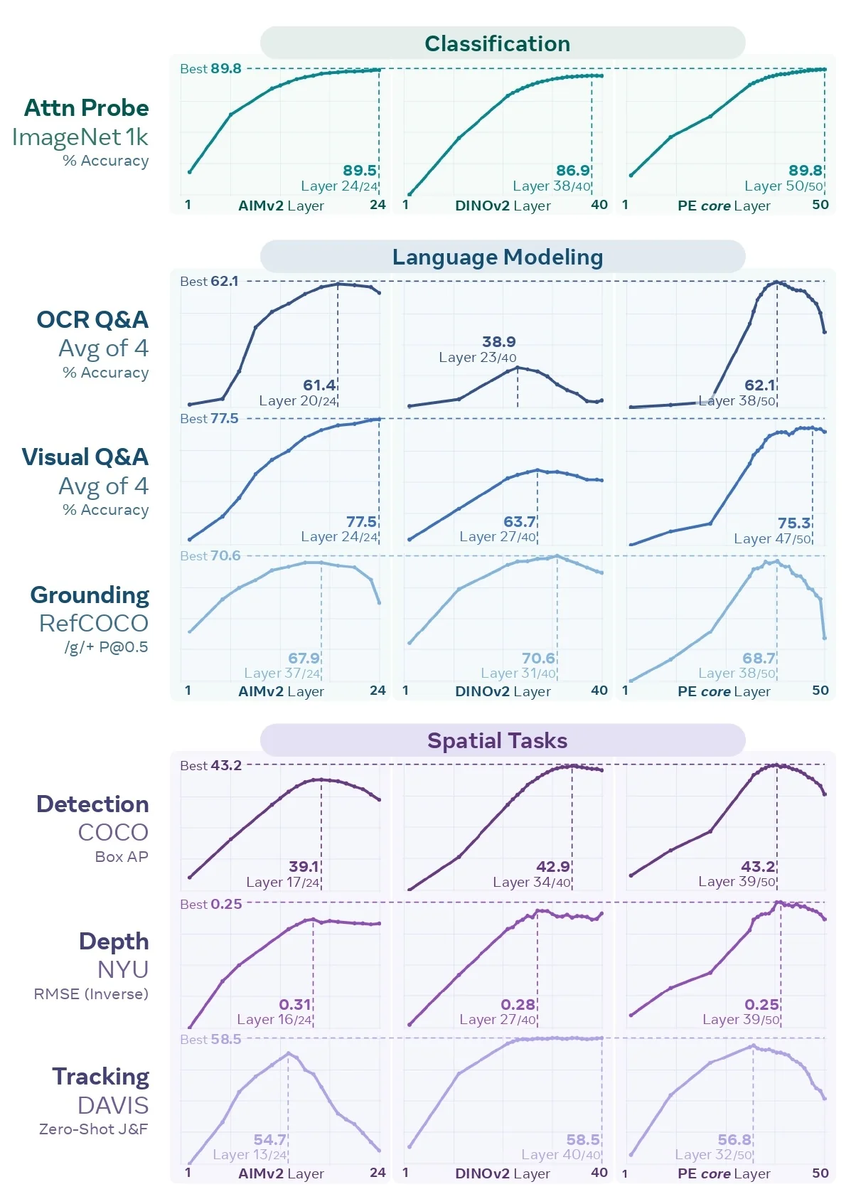
The authors find that a single late-intermediate layer (for example, layer \(L\) near the top of the stack) strikes the best trade-off: earlier layers are too low-level, and the final layer is too spatially collapsed. One might imagine aggregating many layers (as in FPNs), but this increases memory and complexity; instead, PE selects a single strong intermediate layer and, when needed, builds a lightweight multi-scale pyramid from it. In SAM 3, this design is reflected by:
- Extracting tokens from a chosen intermediate layer of the frozen PE backbone.
- Passing the tokens through a shallow FPN-style adapter to obtain the multi-scale features required by the detector and tracker.
This avoids re-training the entire massive backbone while still providing dense, semantically rich feature maps.
Stage 2: alignment tuning and layer selection Once PE Core is trained, it serves as a generic vision encoder whose layers exhibit different strengths. A key empirical finding in the PE paper [48] is that the final layer of a contrastive model is often not the best compromise for downstream tasks: it is highly optimized for global text–image matching, but tends to over-compress spatial detail. In contrast, intermediate layers can provide a better balance between semantics and geometry.
To make this precise, the authors perform a layer-wise probing experiment: for each encoder block \(l\), they freeze PE Core, attach a small task head on top of the features \(z^{(l)}(x)\), and measure performance on semantic tasks (captioning, OCR, VQA) and spatial tasks (self-supervised detection/segmentation). This reveals two “sweet spot” depths:
- A late–intermediate layer \(L_{\mbox{lang}}\) (e.g., block 47 in a 50-block ViT) that performs best on language-aligned tasks.
- An earlier layer \(L_{\mbox{spatial}}\) (e.g., block 41) that preserves more spatial structure and performs best on dense prediction tasks.
Stage 2, alignment tuning, then constructs two specialized variants—PE Language and PE Spatial—by branching from these layers and fine-tuning lightweight heads (and, in the spatial case, the top of the backbone) under regime-specific objectives.
PE Language: visual tokens for multimodal LMs. The PE Language variant adapts PE Core so that its features can be consumed as tokens by a multimodal large language model (MLLM), while preserving the benefits of contrastive pretraining.
- Layer selection and architecture. Instead of using the very last layer of PE Core, the authors branch from the late–intermediate “language-optimal” layer \(L_{\mbox{lang}}\) (e.g., block 47), discarding a few top blocks that are overly specialized for retrieval. A small vision projector (a 2-layer MLP) maps the tokens \(z^{(L_{\mbox{lang}})}(x)\) into the MLLM’s embedding space, forming a sequence of visual tokens. These are concatenated with text tokens and fed into an unfrozen Llama-style MLLM.
-
Training data and objective. PE Language is trained on mixed multimodal data: captioning corpora, OCR-centric datasets, and vision–language QA. The loss is the standard autoregressive next-token prediction on the text side. Gradients backpropagate through the language model, the vision projector, and the top of the vision encoder, aligning the visual tokens with the MLLM’s internal language space.
- Effect of alignment. After alignment tuning, a new layer-wise probe shows that, for the PE Language variant, the final layer now becomes the best-performing layer on language tasks. In other words, alignment tuning “lifts” the strong intermediate representation up to the end of the network while preserving the CLIP-trained trunk.
The resulting PE Language encoder is semantically aligned with text and well suited for tasks where dense geometry is less critical but precise language understanding (e.g., OCR, captioning, VQA) is paramount.
PE Spatial: dense, geometry-aware features for SAM 3. The PE Spatial variant is tailored for dense prediction and is the one used by SAM 3. Its goal is to endow the final-layer tokens with the sharp boundaries and spatial coherence required for segmentation and tracking, without sacrificing the semantics inherited from PE Core.
- Layer selection. PE Spatial branches from the earlier “spatial-optimal” intermediate layer \(L_{\mbox{spatial}}\) of PE Core (e.g., block 41), where the representation still closely tracks object layout and fine geometry. This layer acts as a semantic teacher: its frozen features encode which regions correspond to which concepts, but they are not yet trained to produce explicit masks.
-
Geometric teacher: SAM 2.1 masks. SAM 2.1 is a higher-accuracy variant of SAM 2, trained with stronger augmentation and improved decoders to maximize boundary fidelity. It has no language or concept modeling, but produces exceptionally clean, high-frequency mask logits that capture thin structures and precise edges that CLIP-style contrastive models typically miss.
For each training image \(x\), the authors run SAM 2.1 offline with a dense grid of point prompts (typically hundreds of points spread over the image). For each point, SAM 2.1 outputs one or more mask logits; stacking these over all points yields a 3D tensor \[ m_{\mbox{SAM2.1}}(x) \in \mathbb {R}^{K \times H \times W}, \] where \(K\) indexes the point-prompts / mask slots, and each slice \(m_{\mbox{SAM2.1}}^{(k)}(x) \in \mathbb {R}^{H \times W}\) is a logit mask that is sharply aligned to object boundaries. These masks form a dense, purely geometric teacher: they encode where objects begin and end, including thin structures and occlusion boundaries, but carry no text or concept labels.
-
Student head and dual distillation objective. Starting from PE Core, they fine-tune the upper part of the encoder and attach a shallow dense head to produce a matching tensor \[ m_{\mbox{spatial}}(x) \in \mathbb {R}^{K \times H \times W} \] from the PE Spatial tokens. The dense head is trained to imitate SAM 2.1’s grid of masks for the same set of prompts (same grid, same \(K\)), so that for each mask slot \(k\) and each pixel \((u,v)\), the student is asked to reproduce the teacher’s logit: \[ m_{\mbox{spatial}}^{(k)}(x)[u,v] \approx m_{\mbox{SAM2.1}}^{(k)}(x)[u,v]. \] At the same time, a global pooling head on top of PE Spatial is regularized to stay semantically close to PE Core at depth \(L_{\mbox{spatial}}\). Concretely, for each image \(x\) they minimize \[ \mathcal {L}_{\mbox{sem}} = \lambda _{\mbox{sem}} \,\bigl \| h_{\mbox{spatial}}(x) - h_{\mbox{core}}^{(L_{\mbox{spatial}})}(x) \bigr \|_2^2, \qquad \mathcal {L}_{\mbox{geom}} = \lambda _{\mbox{geom}} \,\mathcal {L}_{\mbox{KD}}\bigl (m_{\mbox{spatial}}(x), m_{\mbox{SAM2.1}}(x)\bigr ), \]
where:
- \(h_{\mbox{core}}^{(L_{\mbox{spatial}})}(x)\) is a global summary (e.g., attention-pooled) from the frozen intermediate teacher layer \(L_{\mbox{spatial}}\) of PE Core.
- \(h_{\mbox{spatial}}(x)\) is the corresponding summary from the PE Spatial student.
- \(m_{\mbox{spatial}}(x)\) are dense mask logits predicted from PE Spatial tokens via the shallow decoder.
- \(\mathcal {L}_{\mbox{KD}}\) is a per-pixel distillation loss (e.g., cross-entropy or KL divergence) that compares teacher and student logits for every mask slot \(k\) and every pixel \((u,v)\).
Intuitively, \(\mathcal {L}_{\mbox{geom}}\) forces the student to reproduce SAM 2.1’s very sharp decision boundaries everywhere in the image: along object edges, across thin structures, and in occluded regions. To succeed, the PE Spatial tokens must organize themselves so that nearby pixels on the same object map to similar features and pixels across boundaries map to clearly separated features. Compared to the original CLIP-only supervision (which only constrains the global embedding), this token-level distillation injects detailed geometric structure into the backbone.
Through this dual distillation, PE Spatial inherits semantics from PE Core (via \(\mathcal {L}_{\mbox{sem}}\)) and boundary precision from SAM 2.1 (via \(\mathcal {L}_{\mbox{geom}}\)). The resulting final-layer tokens are both globally meaningful (for concept prompts and presence prediction) and geometrically sharp (for decoding instance masks and tracking), making PE Spatial an ideal shared backbone for SAM 3’s PCS detector and tracker.
Feature visualizations: geometry–semantics tradeoff The geometry–semantics tradeoff is visible when projecting final-layer features into a 3D color space (PCA followed by LCh mapping). The figure below compares PE variants on example images.
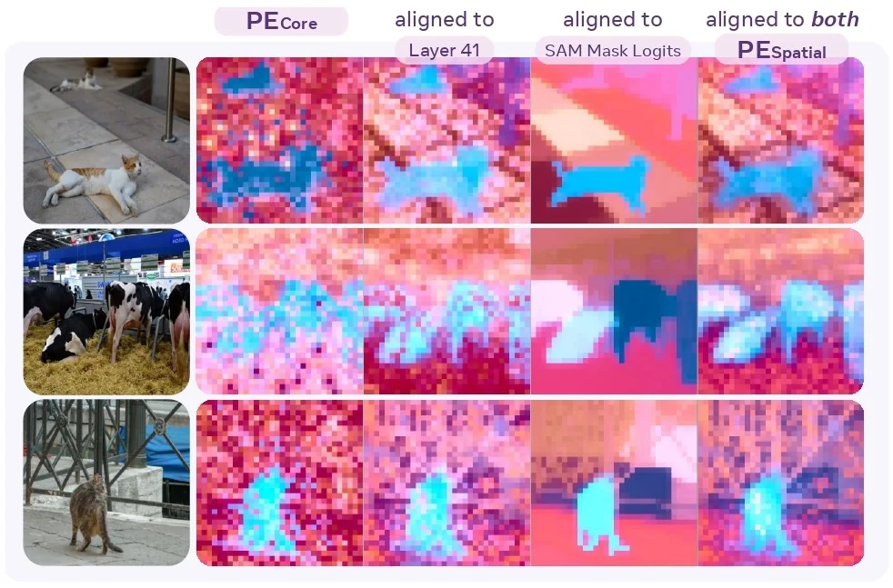
Frozen-feature dense prediction performance Quantitatively, PE Spatial is evaluated as a frozen backbone on a suite of dense prediction tasks: zero-shot tracking (DAVIS), semantic segmentation (ADE20K), and monocular depth estimation (NYUv2). A representative comparison (adapted from the PE paper) is:
| Tracking (DAVIS) \(\uparrow \) | Segm. (ADE20K) \(\uparrow \) | Depth (NYUv2) \(\downarrow \)
| ||||
|---|---|---|---|---|---|---|
| Encoder | Best | Last | Best | Last | Best | Last |
| DINOv2-L | \(58.7\) | \(58.2\) | \(47.3\) | \(47.3\) | \(0.297\) | \(0.308\). |
| DINOv2-g | \(58.5\) | \(58.5\) | \(48.7\) | \(48.4\) | \(0.279\) | \(0.290\). |
| PE Core\(_{\mathrm {G}}\) | \(56.8\) | \(42.8\) | \(41.5\) | \(38.6\) | \(\mathbf {0.249}\) | \(0.309\). |
| PE Spatial\(_{\mathrm {G}}\) | 61.5 | 61.5 | 49.3 | 48.9 | \(0.262\) | 0.275. |
Here, “Best” denotes the best checkpoint encountered during training (highest validation performance), while “Last” denotes the final checkpoint at the end of training.
The gap between PE Core and PE Spatial illustrates the importance of the spatial alignment stage: without it, final-layer features are too semantic and spatially coarse for high-quality segmentation and tracking.
Integration into SAM 3: running example In SAM 3’s architecture (Figure 15.58), the Perception Encoder provides a multi-scale feature pyramid shared by:
- DETR-style concept detector. Consumes PE Spatial features plus text and exemplar tokens to predict concept-conditioned queries, boxes, and masks.
- SAM 2-style tracker. Uses the same PE Spatial features to propagate masklets over time via a memory bank and transformer-based propagation.
To make the flow concrete, consider a single image \(I\) of a crowded street with several red buses and many other objects, and a prompt \(P =\) “red bus”. SAM 3 processes this input as follows.
- 1.
- Feature extraction (PE Spatial). The image \(I\) is passed through PE Spatial, whose ViT backbone produces a single high-resolution feature map at a fixed stride (typically 14 or 16). Because a single-scale feature map is insufficient for detecting objects of very different sizes, SAM 3 converts this map into a multi-scale pyramid \[ \{F^{(s)}\}_{s=1}^{S}, \] where each \(F^{(s)}\) is a feature map at a different spatial resolution. A lightweight FPN-style adapter upsamples the backbone output to create a finer map (stride 4) for small-object and boundary detail, and downsamples it to create coarser maps (stride 32 or 64) for large objects and global context. This yields \(S\) pyramid levels that jointly capture fine geometry and broad semantic cues. The detector and mask head consume all \(\{F^{(s)}\}\) rather than a single PE output because multi-scale context is essential for accurate localization and instance segmentation across a wide range of object sizes.
- 2.
- Prompt encoding. The text “red bus” is tokenized and encoded into a sequence of text embeddings. If exemplars are provided (e.g., a positive box on one bus), ROI pooling over \(F^{(s)}\) plus positional and label embeddings yields exemplar tokens.
- 3.
- Fusion and decoding. A fusion encoder conditions the visual tokens in \(\{F^{(s)}\}\) on the prompt tokens via cross-attention, biasing features toward regions that might be “red buses”. A DETR-style decoder then produces object queries, each predicting a box, a match score to the concept, and a corresponding mask.
- 4.
- Presence gating. A global presence token, operating on PE Spatial’s global context, predicts whether any “red bus” is present in the image. If the presence score is low, all local detections are suppressed; if high, local scores are passed through. This separation between global presence and local localization is directly reflected in the cgF1 metric discussed in the experiments section.
For video, the same PE Spatial backbone is run frame by frame, and its features are shared by the detector and the SAM 2-style tracker, which propagates and periodically re-anchors masklets, as described in the subsequent subsection.
Concept detector and tracker
With the PE Spatial backbone serving as the foundation, SAM 3 constructs its two primary modules: a prompt-conditioned detector and a video tracker.
DETR-style detector conditioned on prompts The SAM 3 detector adapts the standard DETR paradigm [64] to be conditional on open-vocabulary prompts. For each input frame (or image) \(I\), the computation proceeds in three stages.
-
Multi-scale visual features. The PE Spatial backbone is a ViT that, for an input of size \(H \times W\), produces a single grid of patch tokens at stride \(s_{\mbox{PE}}\) (e.g., \(s_{\mbox{PE}} = 16\)). Concretely, the final token grid can be reshaped into a feature map \[ F_{\mbox{PE}} \in \mathbb {R}^{H' \times W' \times D}, \qquad H' = \tfrac {H}{s_{\mbox{PE}}}, \; W' = \tfrac {W}{s_{\mbox{PE}}}, \] where \(D\) is the channel dimension.
Since DETR-style detectors and MaskFormer-style heads benefit from a multi-scale pyramid, SAM 3 adds a lightweight neck (similar to SimpleFPN) on top of \(F_{\mbox{PE}}\). This neck produces a set of \(S\) feature maps \[ \{F^{(s)}\}_{s=1}^S, \qquad F^{(s)} \in \mathbb {R}^{H_s \times W_s \times C}, \] at different strides (e.g., \(4, 8, 16, 32\)), using a combination of \(1\times 1\) convolutions, upsampling, and downsampling. High-resolution levels (\(s=1,2\)) are critical for fine mask boundaries, while coarse levels (\(s=3,4\)) capture large objects and global context. PE Spatial itself is kept frozen during SAM 3 training; all gradients are confined to the neck, fusion encoder, decoder, presence head, and tracker.
-
Prompt encoders. The prompt is encoded into a sequence of prompt tokens that jointly represent the noun phrase and any image exemplars.
-
Text. The noun phrase is tokenized and passed through a text tower, producing a sequence of text embeddings \(\{t_j\}\).
-
Image exemplars. Each exemplar consists of a bounding box \(b\) and a binary label \(\ell \in \{\mbox{pos}, \mbox{neg}\}\). For each exemplar, SAM 3 constructs:
- A position embedding encoding the box coordinates \(b\).
- A label embedding for the sign of the exemplar (include vs. exclude).
- An ROI-pooled feature obtained by pooling PE Spatial features from \(F_{\mbox{PE}}\) (or from an appropriate \(F^{(s)}\)) over the box region.
These components are concatenated and passed through a small Transformer to yield a single exemplar token per box, capturing its spatial location, inclusion/exclusion label, and visual appearance.
The text tokens and exemplar tokens are concatenated into a unified prompt sequence.
-
-
Fusion encoder and DETR decoder. A fusion encoder takes the multi-scale visual tokens derived from \(\{F^{(s)}\}\) and conditions them on the prompt tokens via cross-attention. In each layer, visual tokens attend to the prompt sequence, so the resulting feature maps are explicitly biased toward regions that may match the concept. This design is asymmetric: prompts influence visual features, but visual features do not update the prompt representation, keeping the prompt embedding stable across images.
A DETR-like decoder then uses a set of \(Q\) learned object queries to attend to these prompt-conditioned feature maps and produce object-level predictions. Unlike standard DETR, which predicts over a fixed class vocabulary, each query predicts a binary match score relative to the input concept.
Decoding, losses, and mask prediction Each decoder layer refines a set of \(Q\) object hypotheses. For query \(q_i\) at layer \(\ell \), the head predicts:
- Classification logit. A scalar \(s_i^{(\ell )}\) indicating whether \(q_i\) matches the prompted concept (conditional on the concept being present at all; the global factorization is handled by the presence head).
- Bounding box refinement. A box \((\hat {b}_i^{(\ell )})\) obtained by adding a learned delta to the previous layer’s box prediction, following iterative refinement as in Deformable DETR [827].
Several architectural and loss-design choices are used to make this detector more robust:
- Box-region positional bias. SAM 3 augments attention with box-region positional bias [370]. For an object query associated with a reference box, attention scores to spatial tokens are modulated by a learned function of the relative position between the token and the box (e.g., whether the token lies inside, near the edges, or far outside). This encourages the model to focus its attention on the region likely to contain the object, without resorting to multi-scale deformable attention.
-
Dual supervision from DAC-DETR and Align loss. Training uses Hungarian matching between predicted queries and ground-truth objects, as in DETR, but with two important refinements:
- DAC-DETR [251] (Divide-And-Conquer) splits queries into groups (such as anchor and auxiliary branches) and performs matching in a way that stabilizes training and encourages diverse query utilization. This reduces degenerate behaviors where only a small subset of queries carry most of the signal.
-
The Align loss [62] encourages the classification score to correlate with localization quality: predictions with high IoU to ground-truth boxes are penalized if their classification scores are low, and conversely, high scores are discouraged for low-IoU boxes.
This ties confidence calibration tightly to geometric accuracy, which is crucial in open-vocabulary PCS where false positives are especially harmful.
The total detection loss combines bipartite-matching losses (box regression and classification) with these auxiliary terms.
- MaskFormer-style instance masks. Instance masks are produced by a MaskFormer-style head [99]. A high-resolution pixel embedding map is computed from the top levels of the feature pyramid (e.g., by upsampling \(F^{(1)}\) and fusing with other scales). Each query \(q_i\) is projected into a vector of mask coefficients, and the mask logits for query \(i\) are given by a dot product between these coefficients and the pixel embeddings at each location. This yields a dense mask \(\hat {m}_i \in \mathbb {R}^{H\times W}\) aligned with the input image.
- Handling mask ambiguity. Certain concepts are inherently ambiguous at the mask level (e.g., “wheel” vs. “tire”, or whether to include accessories). To model such ambiguity, the mask head predicts multiple candidate masks per query (e.g., \(K\) variants), each with an associated confidence. During training, the best-matching candidate (in IoU) is used for supervision; at inference time, SAM 3 selects the most confident candidate, or, when needed, aggregates them. This lets the detector represent multiple plausible segmentations for the same object hypothesis.
Alongside instance masks, a separate semantic head aggregates query predictions into a per-pixel binary membership map for the prompted concept, yielding the semantic PCS output.
Presence head: decoupling recognition and localization A central design idea in SAM 3 is to decouple recognition (“is the concept present at all?”) from localization (“where are its instances?”). The decoder’s object queries are inherently local, making them well suited for localization but less ideal for deciding global presence, which may depend on subtle contextual cues.
SAM 3 introduces a learned global presence token whose sole responsibility is to predict whether the noun phrase NP is present anywhere in the input. Formally, the model factorizes the classification probability as \begin {equation} p(q_i \mbox{ matches NP}) = p\bigl (q_i \mbox{ matches NP} \mid \mbox{NP is present in input}\bigr )\cdot p(\mbox{NP is present in input}), \label {eq:chapter15_sam3_presence_factorization} \end {equation} where:
- \(p(\mbox{NP is present in input})\). A single scalar predicted by the presence token using global context (e.g., pooled features over the entire image or clip). This score is shared by all object queries and acts as a global gate: if it is low, all local detections are suppressed.
- \(p(q_i \mbox{ matches NP} \mid \mbox{NP is present in input})\). Predicted by each proposal query \(q_i\) from its local evidence and geometry, conditioned on the concept being present.
SAM 3 employs a decoupled supervision strategy. The presence head is always supervised with binary cross-entropy based on image-level labels (present vs. absent). The local object queries \(q_i\) receive box/mask supervision and matching gradients only on images where the concept is present. On negative images, they learn simply that all queries should remain “background” under the presence gate, rather than being forced to hallucinate boxes for a missing concept. At evaluation time, the global presence score contributes to the IL_MCC term in cgF1, while query-level localization quality drives pmF1.
Image exemplars and interactive refinement SAM 3 extends SAM and SAM 2 by allowing exemplars to define or refine the concept, not just select a single instance. Given a positive bounding box on one object (e.g., a dog), the detector interprets the exemplar as “find all objects that look like this dog”. Negative exemplars exclude specific visual modes (e.g., a different fish species) from the concept. As illustrated in Figure 15.63, adding a negative exemplar on an undesired fish species removes that sub-concept from the predicted masks while preserving the intended striped fish.
During inference, exemplars are encoded as described above and concatenated with text tokens into a single prompt token sequence. By adding exemplars iteratively, users can refine both recognition (which visual mode corresponds to the phrase) and localization (which pixels belong to the intended instances).
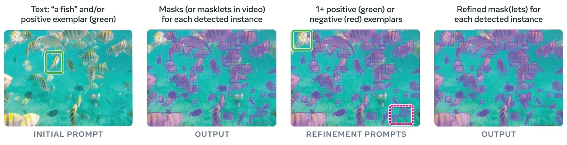
Video PCS: detector–tracker factorization For videos, SAM 3 combines its concept detector with a SAM 2-style tracker. Given a video and prompt \(P\), the detector finds concept instances on each frame while the tracker propagates existing masklets forward in time. Let \(I_t\) be the frame at time \(t\), \(M_{t-1}\) the set of masklets from frame \(t-1\), and \(O_t\) the set of newly detected objects at frame \(t\). SAM 3 defines \begin {equation} \hat {M}_t = \mbox{propagate}(M_{t-1}), \quad O_t = \mbox{detect}(I_t, P), \quad M_t = \mbox{match_and_update}\bigl (\hat {M}_t, O_t\bigr ). \label {eq:chapter15_sam3_tracking_update} \end {equation} Here:
- Propagation. The tracker predicts the new locations \(\hat {M}_t\) of previously tracked objects using a single-frame propagation step similar to SAM 2: track tokens attend to the current PE Spatial features and a memory bank of past features to update each masklet.
- Detection. The detector runs on \(I_t\) with prompt \(P\) to find new instances \(O_t\) that match the concept, including objects that enter the scene or were previously missed.
- Matching and updating. A simple IoU-based matching function associates propagated masklets \(\hat {M}_t\) with current detections \(O_t\), forming the updated set of masklets \(M_t\). New detections that are unmatched spawn new masklets.
To improve temporal robustness, SAM 3 introduces two strategies:
- Masklet detection score. For each masklet, a temporal score accumulates how consistently it has been re-matched to detector outputs over a sliding window. Masklets whose detection score falls below a threshold are suppressed, reducing drift and spurious tracks.
- Periodic re-prompting. At regular intervals, the tracker is re-anchored using high-confidence detector masks: the tracker’s internal state for a masklet is refreshed from the detector’s current prediction. This prevents the memory bank from drifting away from the true object when occlusions or appearance changes occur.
As in the image detector, the mask decoder can output multiple candidate masks per tracked object along with confidences; SAM 3 then selects the most confident mask on each frame, which helps resolve per-frame ambiguities in cluttered or low-contrast regions.
Instance refinement with visual prompts After initial concept detection and tracking, SAM 3 supports finer instance-level refinement with PVS-style visual prompts (points, boxes) in the SAM 2 fashion. A user can:
- Refine a masklet. Provide positive and negative clicks on a specific object; SAM 3 encodes the clicks and runs the mask decoder to adjust the mask on that frame.
- Propagate refinements. In video, the refined mask is propagated across the entire sequence to update the masklet consistently.
In many practical workflows, the user first runs PCS to discover all instances of a concept, then selects one masklet and refines it with PVS-style prompts, effectively turning PCS into single-object segmentation or tracking for that chosen instance. This design unifies concept-level prompting (PCS) with instance-level visual refinement (PVS), providing both global coverage and local precision.
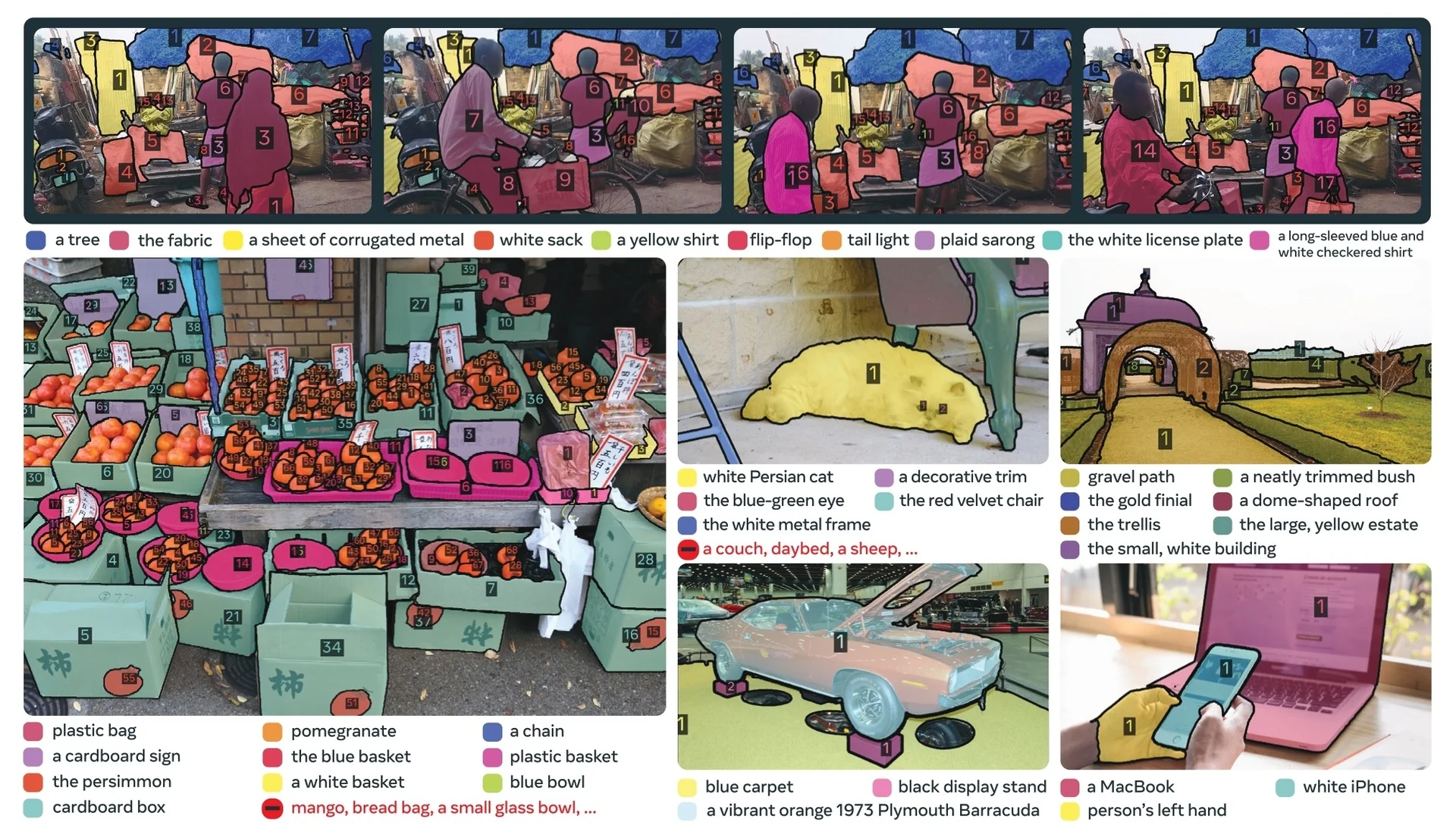
Training and data
Training stages SAM 3 is trained in four stages [65].
- Perception Encoder pre-training. The PE backbone is trained on large-scale vision tasks (contrastive image and video pretraining with alignment tuning) to learn strong general visual representations before being used for PCS.
- Detector pre-training. The DETR-style detector is trained with text and exemplar prompts on SA-Co and related data, supervised with both box and mask objectives and the presence head, so that it can perform open-vocabulary detection and segmentation conditioned on concept prompts.
- Detector fine-tuning. The detector is further fine-tuned on curated subsets and external datasets (e.g., LVIS, COCO, ADE-847) for PCS and related tasks, balancing open-vocabulary behavior with strong performance on standard benchmarks.
- Tracker training. With the backbone frozen, the tracker is trained on video PCS data to propagate masklets and maintain identities, using SAM 2-style propagation losses and consistency objectives.
Data engine and SA-Co dataset Achieving strong PCS performance requires a large, diverse dataset over many domains. SAM 3 introduces a model- and human-in-the-loop data engine (see the below figure) that iteratively improves both the dataset and the model.
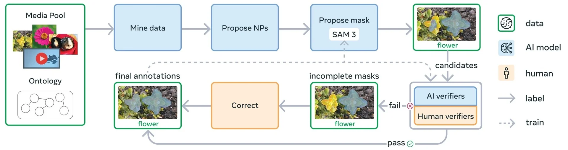
The data engine operates in phases.
- Phase 1: Human verification. Initial image–NP pairs are generated using SAM 2 plus an open-vocabulary detector, and all verification is done by humans, producing the first SA-Co/HQ subset with millions of pairs.
- Phase 2: Human + AI verification. Human labels from Phase 1 are used to fine-tune Llama-based AI verifiers for mask quality and exhaustivity, roughly doubling annotation throughput. Hard negative NPs are mined adversarially to challenge SAM 3.
- Phase 3: Scaling and domain expansion. AI models mine increasingly difficult cases and broaden coverage to many visual domains, while the ontology is used to expand long-tail concept coverage.
- Phase 4: Video annotation. The pipeline is extended to videos, using SAM 3 to propose masklets that are then verified and corrected, focusing human effort on crowded scenes and likely tracking failures.
From this process, the authors build several datasets for training and evaluation [65].
- SA-Co/HQ. High-quality image PCS data with about \(5.2\)M images and \(4\)M unique noun phrases.
- SA-Co/SYN. A synthetic dataset with about \(38\)M phrases and \(1.4\)B masks, generated using a mature data engine without human involvement.
- SA-Co/EXT. Fifteen external datasets with existing instance masks, enriched with hard negatives using the ontology.
- SA-Co/VIDEO. About \(52.5\)K videos and \(24.8\)K unique noun phrases, forming approximately \(134\)K video–NP pairs.
The SA-Co benchmark for evaluation contains \(207\)K unique phrases and over \(3\)M media–phrase pairs, spanning multiple splits (Gold, Silver, Bronze, Bio, and VEval) with varying levels of redundancy and domain focus. With this architecture, training protocol, and data engine in place, the authors next quantify how well SAM 3 performs on PCS across images and videos and how each design choice contributes to the final performance.
Experiments and ablations
Evaluation metrics: why open-vocabulary PCS needs new metrics Conventional detection metrics such as AP (Average Precision) were developed for closed-set detection, where the model predicts over a fixed label set and is not judged on its ability to refuse arbitrary new phrases. In Promptable Concept Segmentation (PCS), every query phrase can be novel, and evaluation must answer two separate questions:
- 1.
- Presence: does the concept appear at all in this image or video?
- 2.
- Localization: given that it does, are all instances segmented accurately?
Standard AP collapses these into a single ranking-based score. A model that often hallucinates confident detections for concepts that are not present can still achieve a seemingly good AP if it ranks detections well on positive images. This is misaligned with the real PCS goal: “Do you know when the concept is here, and when it is, can you segment it well?”
SAM 3 therefore evaluates PCS using a calibration-sensitive metric called classification-gated F1 (cgF1) [65], which explicitly factorizes the task into a localization component and a presence component.
Localization: positive micro-F1 (pmF1).
A standard F1 score is defined from precision and recall, \[ \mathrm {F1} = \frac {2 \,\mathrm {Precision} \cdot \mathrm {Recall}}{\mathrm {Precision} + \mathrm {Recall}}, \] where precision and recall are computed from counts of true positives (TP), false positives (FP), and false negatives (FN). There are two common aggregation schemes:
- Per-example (macro) F1: compute F1 separately for each image, then average.
- Micro-F1: first sum TP, FP, and FN across all examples, then compute a single F1 from the totals.
pmF1 is a micro-F1 over instances, restricted to positive media–phrase pairs. Concretely:
- We consider only media–phrase pairs for which the concept is known to be present (at least one ground-truth instance exists).
- For each such pair, predicted instances (boxes + masks) are matched to ground-truth instances using an IoU-based one-to-one matching.
- Over all positive pairs, we accumulate instance-level counts \[ \mathrm {TP}_\mbox{pos},\quad \mathrm {FP}_\mbox{pos},\quad \mathrm {FN}_\mbox{pos}, \] and define \[ \mathrm {Precision}_\mbox{pos} = \frac {\mathrm {TP}_\mbox{pos}}{\mathrm {TP}_\mbox{pos} + \mathrm {FP}_\mbox{pos}}, \qquad \mathrm {Recall}_\mbox{pos} = \frac {\mathrm {TP}_\mbox{pos}}{\mathrm {TP}_\mbox{pos} + \mathrm {FN}_\mbox{pos}}, \] \[ \mathrm {pmF1} = \frac {2 \,\mathrm {Precision}_\mbox{pos} \cdot \mathrm {Recall}_\mbox{pos}} {\mathrm {Precision}_\mbox{pos} + \mathrm {Recall}_\mbox{pos}}. \]
The crucial point is what pmF1 ignores: it does not see any media–phrase pairs where the concept is absent. It answers only:
“When the concept truly appears, how accurately do I detect and segment its instances?”
Presence hallucinations on negative images are handled separately.
Presence classification: image-level MCC (IL_MCC).
To measure whether the model correctly decides if a concept is present, SAM 3 uses an image-level Matthews Correlation Coefficient (MCC) over all media–phrase pairs. For each pair, the ground truth provides a binary label \[ y \in \{0,1\} \quad (\mbox{absent/present}), \] and the model predicts \(\hat {y} \in \{0,1\}\) based on its global presence head and query scores. This yields four pair-level counts: \[ \mathrm {TP},\ \mathrm {TN},\ \mathrm {FP},\ \mathrm {FN}, \] and IL_MCC is given by \[ \mathrm {IL\_MCC} = \frac {\mathrm {TP} \cdot \mathrm {TN} - \mathrm {FP} \cdot \mathrm {FN}} {\sqrt {(\mathrm {TP}+\mathrm {FP})(\mathrm {TP}+\mathrm {FN})(\mathrm {TN}+\mathrm {FP})(\mathrm {TN}+\mathrm {FN})}}. \]
MCC can be viewed as a correlation coefficient for binary classification: it is \(1\) for perfect predictions, \(0\) for random guessing or a constant classifier, and \(-1\) for perfectly wrong predictions. It is chosen here for two reasons:
- Robust to class imbalance. SA-Co contains far more negative than positive pairs. A trivial classifier that always predicts “absent” can achieve high raw accuracy, but its MCC stays near \(0\). MCC therefore prevents models from exploiting imbalance by always refusing.
- Symmetric treatment of FP and FN. IL_MCC decreases both when the model hallucinates concepts (many FP on negatives) and when it misses obvious ones (many FN on positives). Both failure modes matter for PCS deployment.
Intuitively, IL_MCC answers:
“Across all images and phrases, how strongly are my presence predictions correlated with reality, after accounting for imbalance and both kinds of mistakes?”
Combined metric: classification-gated F1 (cgF1).
cgF1 combines these two orthogonal requirements into a single scalar: \begin {equation} \mathrm {cgF1} = 100 \times \mathrm {pmF1} \times \mathrm {IL_MCC}. \label {eq:chapter15_sam3_cgF1} \end {equation} This multiplicative design acts as a harsh gate. It forces a model to be simultaneously effective at:
- Localization (high pmF1): accurately segmenting instances when the concept is actually present.
- Calibration (high IL_MCC): reliably predicting “absent” when the concept is missing.
Consider a “hallucination-prone” model that segments every cat perfectly (pmF1 \(\approx 1.0\)) but also incorrectly claims a cat exists in every empty room (IL_MCC \(\approx 0\)). Its final cgF1 will collapse to near zero. This ensures that for open-vocabulary deployment, the model learns that silence is golden: it must confidently refuse to segment irrelevant inputs. Conversely, a conservative model that almost never hallucinates (high IL_MCC) but misses many true instances (low pmF1) will also obtain a low cgF1.
cgF1 is thus directly aligned with the core PCS requirement of jointly reliable recognition (“is the concept here?”) and segmentation (“if so, where and how well?”). Finally, SA-Co/Gold provides three independent human annotation variants per phrase. To account for semantic and boundary ambiguity, oracle scores compare model predictions against all variants and take the best match, so that models are not penalized for choosing one reasonable interpretation among several.
Image PCS with text prompts: large gains over prior work SAM 3 is evaluated on instance segmentation, box detection, and semantic segmentation for a wide variety of natural language prompts [65]. Baselines include OWLv2, Grounding DINO, LLMDet, Gemini 2.5, APE, and DINO-X. Three high-level takeaways emerge:
- Open-vocabulary PCS on SA-Co. On the SA-Co/Gold split, SAM 3 attains a cgF1 of 53.6, more than doubling the performance of OWLv2\(^\star \) (cgF1 \(\sim \)26). This corresponds to roughly 74% of measured human performance. Improvements are even larger on SA-Co Silver, Bronze, and Bio.
- Closed-vocabulary performance. Zero-shot LVIS mask AP is 48.5, which is notable because SAM 3 is not optimized for LVIS and yet surpasses prior CLIP-based detectors and approaches the supervised performance of specialist models from 2022–2023.
- Open-vocabulary semantic segmentation. On ADE-847, PascalConcept-59, and Cityscapes, SAM 3 outperforms APE—a strong specialist for open-vocabulary semantic segmentation—demonstrating that the PCS machinery generalizes from instance to pixel-wise semantics.
Qualitative comparisons in Figure 15.57 illustrate that SAM 3 handles long-tail concepts (“cheesecloth”, “toilet roll holder”) and cluttered scenes that confuse previous systems such as OWLv2 and Grounding DINO.
Few-shot adaptation and exemplar prompting Few-shot transfer is evaluated on ODinW13 and RF-100VL using their native labels as prompts. Fine-tuned without mask losses, SAM 3 achieves state-of-the-art 10-shot detection, outperforming Gemini’s in-context learning and specialist detectors such as Grounding DINO.
A particularly compelling aspect is the impact of exemplar prompts. With only a single positive exemplar:
- SAM 3 substantially outperforms T-Rex2 on COCO, LVIS, and ODinW.
- Joint text+exemplar prompting consistently produces the strongest results.
This suggests that SAM 3’s prompt-conditioning architecture effectively fuses appearance cues (exemplars) with semantic cues (text), enabling fine-grained discrimination between visually similar subcategories.
Efficiency of PCS vs. PVS prompting One of the motivating hypotheses for SAM 3 is that PCS is fundamentally more interaction-efficient than classical PVS. In PVS (as in SAM 2), each object typically requires an explicit prompt (point, box, or mask). PCS, by contrast, uses a single semantic prompt to discover all instances of a concept simultaneously.
This hypothesis is validated on SA-Co/Gold, where cgF1 is plotted against the number of interactive box prompts:
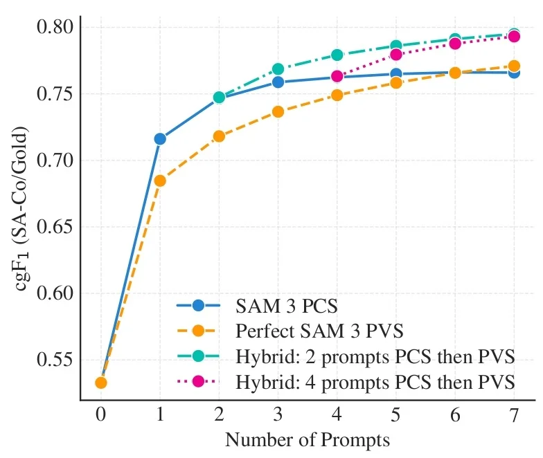
The trends are striking:
- PCS achieves \(\sim \)0.72 cgF1 with just one prompt. For a single prompt, PCS already outperforms a PVS baseline (roughly \(\sim \)0.68 cgF1 at one box prompt), and this PCS level typically requires four to five PVS prompts in SAM 2-style annotation.
- PVS scales linearly with the number of objects. For scenes with many instances (e.g., “all screws on the table”), PVS becomes prohibitively costly, whereas PCS remains constant.
- Hybrid prompting delivers the peak performance (\(\sim \)0.80 cgF1). Use one PCS prompt to retrieve most instances, then refine with 1–2 visual prompts where needed.
Domain adaptation and data engine ablations The SAM 3 data engine produces both human-verified and synthetic annotations. To study domain adaptation, the authors evaluate on a Food-domain subset using three data sources: high-quality human annotations (HQ), synthetic annotations from mature SAM 3 teachers (SYN), and naive pseudo-labels (PL).
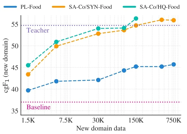
Three practical insights emerge:
- Quality matters as much as quantity. SYN data approaches HQ performance, both reaching cgF1 \(\sim \)56 with sufficient training volume.
- Verification is essential. PL data, without verification, plateaus early around cgF1 \(\sim \)45, underscoring that naive pseudo-labeling is insufficient for open-vocabulary tasks.
- Teacher models can self-scale. When paired with an AI verifier, a strong SAM 3 model can bootstrap high-quality synthetic data for new domains, reducing human annotation cost.
Ablations: identifying key components A series of ablations isolates which design decisions most affect PCS performance:
- Presence head (improves cgF1 by \(\sim \)3.5). Removing the global presence token causes the model to hallucinate concepts more often, lowering IL_MCC and reducing cgF1. This confirms that separating global recognition from local localization is critical.
- Hard-negative prompts (improves cgF1 by \(\sim \)2.1). Including adversarially mined negative noun phrases (e.g., “nail” when querying “screw”) is essential for discriminating fine-grained concepts.
- Ambiguity modeling. Allowing the mask decoder to output multiple candidate masks improves robustness on SA-Co/Gold, where human annotators legitimately disagree about which pixels belong to a concept.
- Backbone capacity (PE Spatial). Upgrading to the Perception Encoder boosts both PCS and PVS performance. Compared to SAM 2’s original encoder, PE Spatial yields significantly stronger tracking, better fine detail, and improved open-vocabulary grounding.
Collectively, these experiments validate the core design of SAM 3: a well-calibrated presence classifier, strong spatial-semantic features from PE, concept-level prompting, and ambiguity-aware mask decoding together produce a substantial leap in open-vocabulary segmentation and tracking.
Limitations and future directions
Despite its strong performance, SAM 3 has several limitations that also suggest promising directions for future work.
Language complexity and reasoning SAM 3 is intentionally restricted to simple noun phrases. It is not designed to handle long referring expressions or prompts requiring complex reasoning (e.g., “the person holding the red umbrella but not standing on the stairs”). While the authors show that SAM 3 can be combined with a Multimodal Large Language Model (MLLM) to parse such queries into simpler noun phrases and concept prompts, this is handled outside the core SAM 3 architecture. A natural next step is tighter integration between PCS models and MLLMs so that reasoning and segmentation are trained jointly.
Ambiguity and annotation effort Even with three annotations per phrase and an ambiguity-aware evaluation protocol, some prompts remain intrinsically ambiguous or ungroundable. The data engine partially mitigates this by allowing annotators to reject such phrases, but this requires substantial human effort and careful guideline design. Future work could explore uncertainty-aware prompting, where the model can explicitly flag phrases it cannot reliably ground.
Domain and modality coverage SA-Co covers many visual domains, but performance still varies across them, and specialized domains (e.g., medical imaging, scientific microscopy) may require dedicated data collection and domain-specific ontology expansions. Extending PCS to additional modalities (e.g., 3D scenes, multi-view setups) or to richer temporal reasoning (beyond short videos) remains an open research area.
Computational cost and deployment Although SAM 3 is optimized for efficiency—running in about \(30\) ms per image with \(100+\) detected objects on an H200 GPU and near real-time for a few concurrent video objects—deployment at scale still requires substantial compute and memory. Lightweight variants or distillation schemes, possibly leveraging concept-specific student models, could make PCS more accessible in resource-constrained settings.
Compositionality and structured prompts Finally, SAM 3 treats each noun phrase largely independently, without explicit modeling of compositional structure across multiple prompts (e.g., intersecting or subtracting concepts). Interactive exemplars partially address this, but richer structured prompting interfaces and corresponding model architectures could better exploit the compositional nature of language and concepts.