Lecture 8: CNN Architectures I

8.1 Introduction: From Building Blocks to SOTA CNNs

Convolutional Neural Networks (CNNs) have revolutionized computer vision by providing state-of-the-art results in image classification, object detection, and many other tasks. While previous chapters introduced the core building blocks of CNNs—convolutional layers, activation functions, normalization techniques, and pooling layers—the question remains: how do we structure these components into effective architectures?

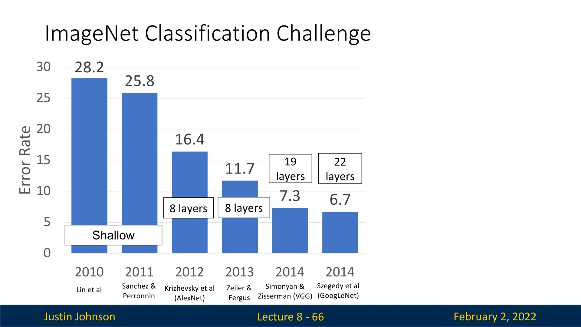
This chapter explores the historical progression of CNN architectures, focusing on key models that have shaped modern deep learning. We ground our discussion in the ImageNet Large Scale Visual Recognition Challenge (ILSVRC), which has served as a driving force for innovation in deep learning-based image classification.

8.2 AlexNet

In 2012, a breakthrough in the field of computer vision—and the winner of the ImageNet classification challenge—was AlexNet [307]. While modern architectures are significantly deeper, AlexNet marked the beginning of deep convolutional networks. It accepted input images of spatial dimensions \(227 \times 227\), with three color channels, leading to an input tensor shape of \(3 \times 227 \times 227\) per image, and a total input batch shape of \(N \times 3 \times 227 \times 227\).

AlexNet consisted of:

• Five convolutional layers, interleaved with max pooling layers.
• Three fully connected layers, finalizing the classification with a softmax output.
• ReLU non-linearity, one of the first architectures to introduce it.
• Local Response Normalization (LRN), a now obsolete normalization technique used before BatchNorm.
• Multi-GPU training, splitting the model across two NVIDIA GTX 580 GPUs, each with only 3GB of memory.

Despite its relatively simple design, AlexNet was hugely influential, accumulating over 100,000 citations since its publication.

This makes it one of the most cited works in modern science, surpassing even landmark research in information theory and fundamental physics.

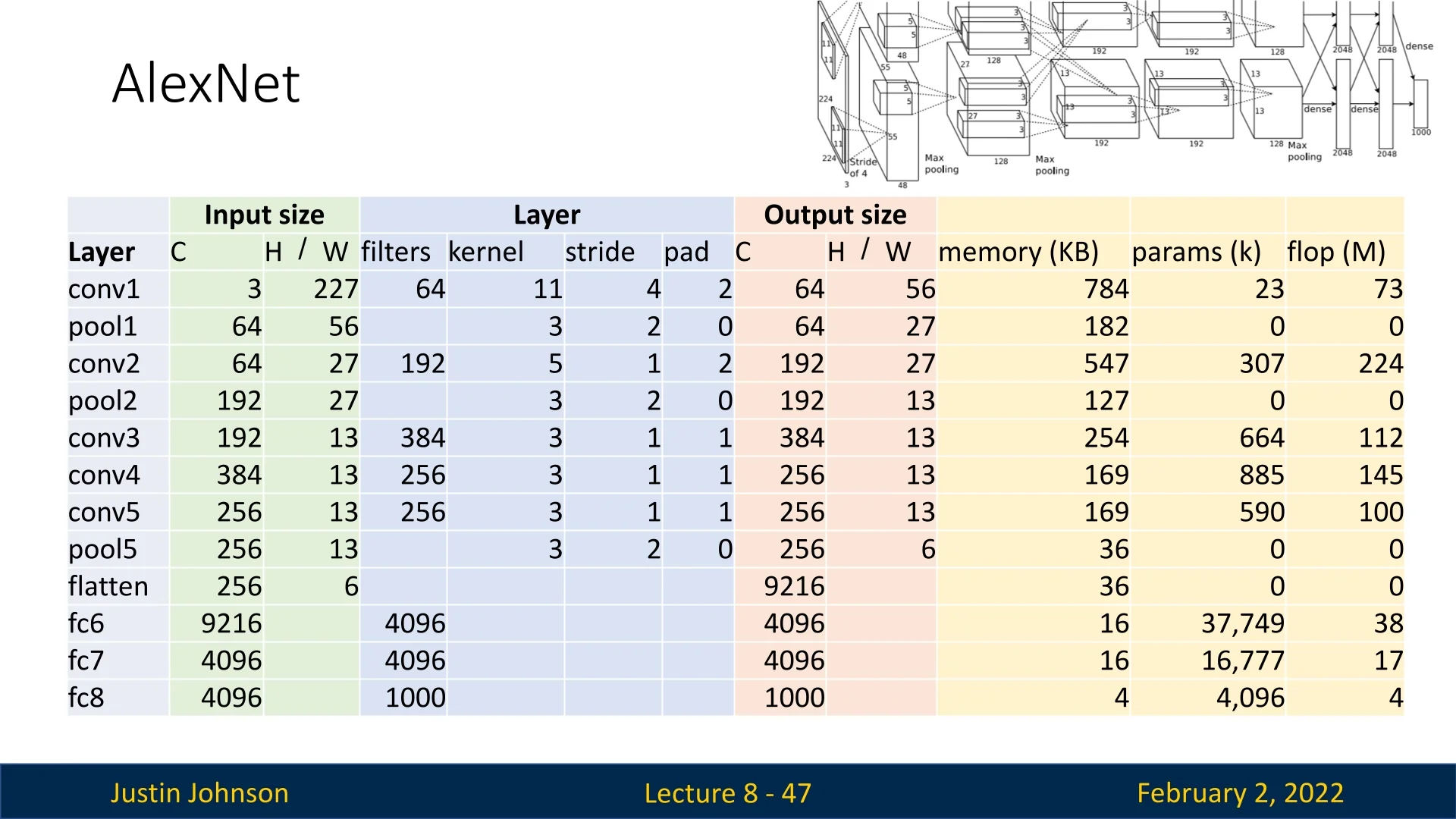
8.2.1 Architecture Details

Let us analyze AlexNet layer by layer, focusing on output dimensions, memory consumption, and computational cost.

First Convolutional Layer (Conv1) The first convolutional layer has \(C_{\mbox{out}} = 64\) filters, kernel size \(K = 11 \times 11\), stride \(S = 4\), and padding \(P = 2\). The output spatial size is computed as:

\begin {equation} W' = \frac {W - K + 2P}{S} + 1 = \frac {227 - 11 + 2(2)}{4} + 1 = 56 \end {equation}

Thus, the output tensor shape is \(64 \times 56 \times 56\).

Memory Requirements Assuming 32-bit floating-point representation (4 bytes per element), the output tensor storage requirement is:

\begin {equation} \frac {(C_{\mbox{out}} \times H' \times W') \times 4}{1024} = \frac {(64 \times 56 \times 56) \times 4}{1024} = 784 \mbox{KB} \end {equation}

Number of Learnable Parameters The weight tensor shape is \(C_{\mbox{out}} \times C_{\mbox{in}} \times K \times K = 64 \times 3 \times 11 \times 11\), with an additional bias term per channel:

\begin {equation} \mbox{Total Params} = (64 \times 3 \times 11 \times 11) + 64 = 23,296 \end {equation}

Computational Cost Each output element requires a convolution with a \(C_{\mbox{in}} \times K \times K\) receptive field, leading to the following Multiply-Accumulate operations (MACs):

\begin {equation} \mbox{#MACs} = (C_{\mbox{out}} \times H' \times W') \times (C_{\mbox{in}} \times K \times K) \end {equation}

\begin {equation} = (64 \times 56 \times 56) \times (3 \times 11 \times 11) = 72,855,552 \approx 78M \mbox{ MACs} \end {equation}

Note: In practice, 1 MAC = 2 FLOPs, since each multiply-accumulate consists of both a multiplication and an addition.

Max Pooling Layer The first pooling layer follows the ReLU activation and has a \(3 \times 3\) kernel with stride \(S = 2\), reducing the spatial size:

\begin {equation} W' = \lfloor (W - K) / S + 1 \rfloor = \lfloor (56 - 3) / 2 + 1 \rfloor = 27 \end {equation}

Thus, the output tensor shape is \(64 \times 27 \times 27\).

Memory and Computational Cost

• Memory: \(64 \times 27 \times 27 \times 4 / 1024 = 182.25\) KB.

• MACs: Since pooling takes only a maximum over a \(3 \times 3\) window, the cost is:

  \begin {equation} (C_{\mbox{out}} \times H' \times W') \times (K \times K) = (64 \times 27 \times 27) \times (3 \times 3) = 0.4M \mbox{ MACs}. \end {equation}

Max pooling is computationally inexpensive compared to convolutions.

8.2.2 Final Fully Connected Layers

The final three layers form a Multi-Layer Perceptron (MLP):

• Flatten Layer: Flattens the \(256 \times 6 \times 6\) tensor into a 9216-dimensional vector.
• First FC Layer: Maps 9216 to 4096 neurons.
• Second FC Layer: Maps 4096 to another 4096 neurons.
• Final FC Layer: Maps 4096 to 1000 output classes (ImageNet categories).

Computational Cost For the first fully connected layer:

\begin {equation} \mbox{FC Params} = (C_{\mbox{in}} \times C_{\mbox{out}}) + C_{\mbox{out}} \end {equation}

\begin {equation} = (9216 \times 4096) + 4096 = 37,725,832 \end {equation}

\begin {equation} \mbox{#MACs} = 9216 \times 4096 = 37,748,736. \end {equation}

The process continues for the other FC layers, culminating in a final output of 1000 neurons for classification.

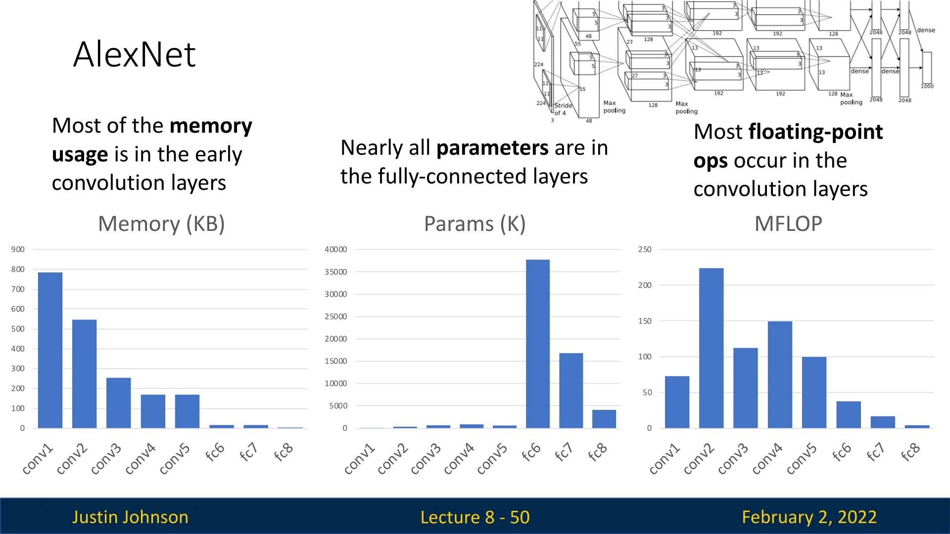
8.2.3 Key Takeaways from AlexNet

• The memory footprint is largest in the early convolutional layers.
• Nearly all parameters are stored in the fully connected layers.
• Most computational cost (FLOPs) occurs in convolutional layers.

8.2.4 ZFNet: An Improvement on AlexNet

In 2013, most competitors in the ImageNet challenge used CNNs following AlexNet’s success. The winner, ZFNet [752], was essentially a refined, larger version of AlexNet.

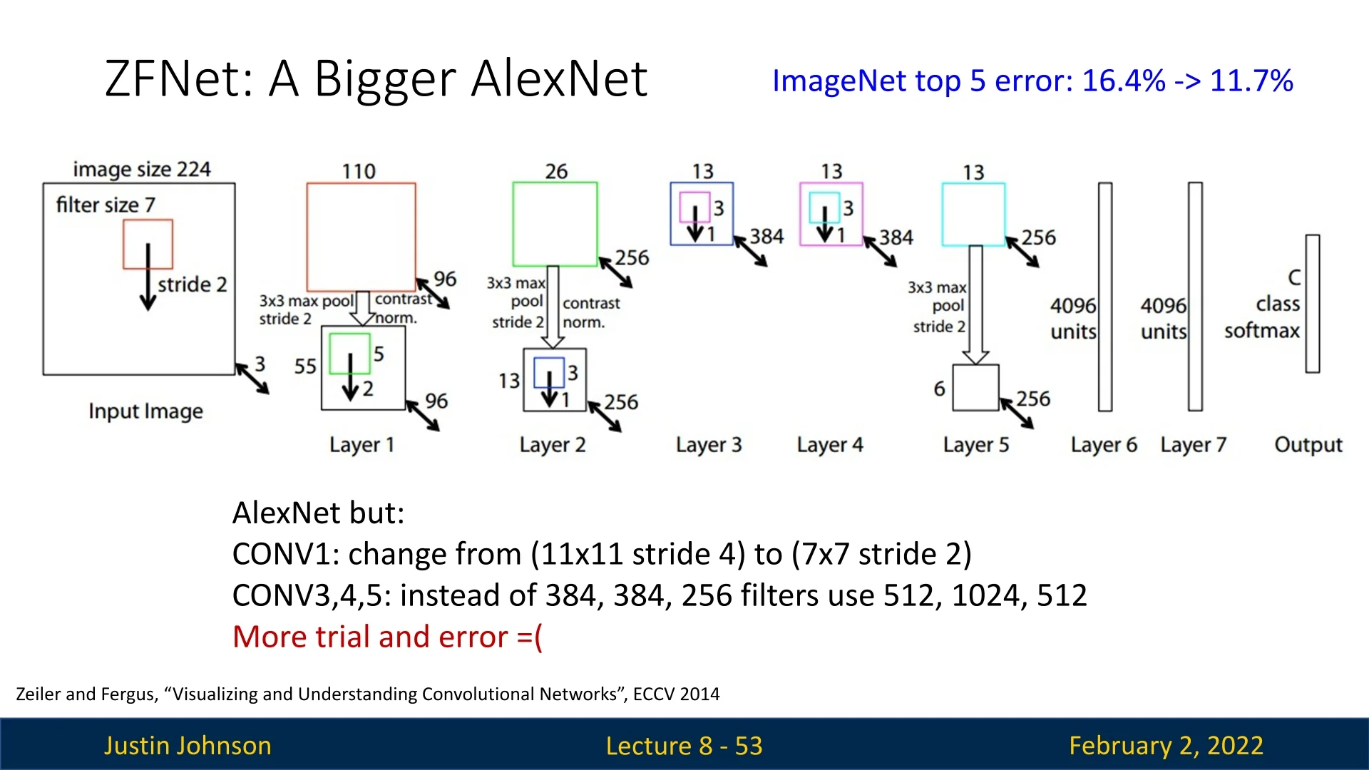
Key Modifications in ZFNet

• The first convolutional layer was adjusted to use a \(7 \times 7\) kernel with stride 2, instead of \(11 \times 11\) with stride 4 in AlexNet. This resulted in finer spatial resolution in early layers.
• Increased number of parameters and computation, leading to improved performance.

The main lesson from AlexNet and ZFNet: larger networks tend to perform better, but architecture refinement is critical.

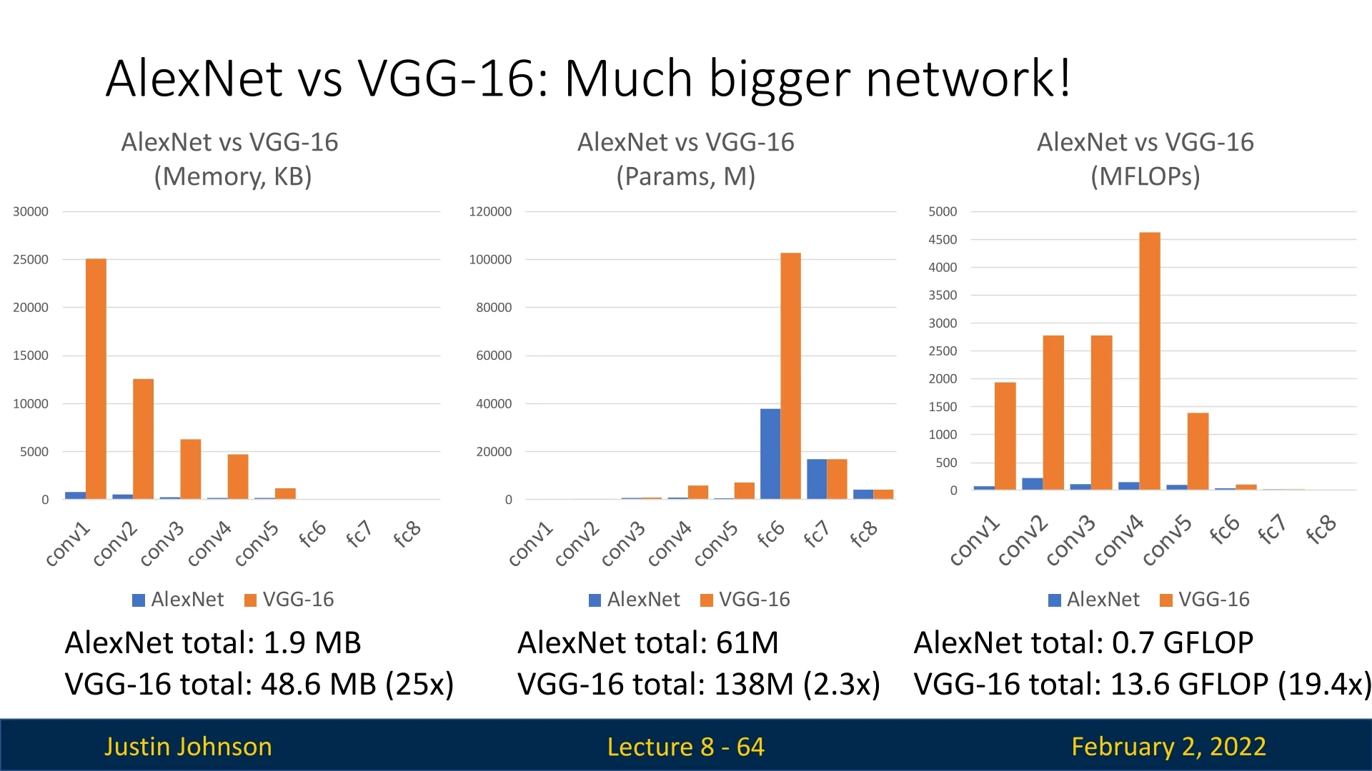
8.3 VGG: A Principled CNN Architecture

Historical Context. Proposed in the 2014 ImageNet challenge by Oxford’s Visual Geometry Group ([572]), VGG demonstrated the power of systematically deepening CNNs. In contrast to ad-hoc predecessor designs like AlexNet, VGG introduced a uniform blueprint for increasing depth using only small kernels and structured downsampling.

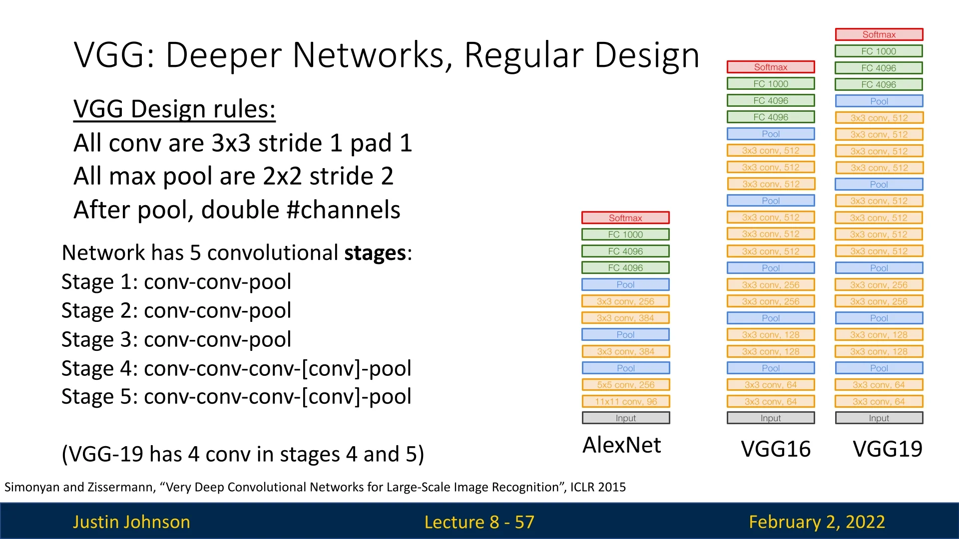
Core Design Principles. VGG’s architecture rests on three simple rules:

1.

All convolutions are \(\,3\times 3\), stride=1, pad=1.

2.

All pooling is \(\,2\times 2\) max-pool with stride=2.

3.

After each pool, the number of channels doubles.

These guidelines enabled much deeper networks than earlier CNNs, yet kept computations relatively manageable.

8.3.1 Network Structure

Five hierarchical stages group VGG’s convolutional layers:

• Stages 1–3: \([\,\mathrm {conv}\!-\!\mathrm {conv}\!-\!\mathrm {pool}\,]\).
• Stages 4–5: \([\,\mathrm {conv}\!-\!\mathrm {conv}\!-\!\mathrm {conv}\!-\![\mathrm {conv}]\!-\!\mathrm {pool}\,]\).

Popular variants are:

• VGG-16 with 16 total convolutional layers,
• VGG-19 with 19 layers (extra conv in stages 4,5).

8.3.2 Key Architectural Insights

Small-Kernel Convolutions (\(3\times 3\))

VGG replaces larger kernels (e.g. \(5\times 5\), \(7\times 7\)) with multiple \((3\times 3)\) layers in sequence:

• Fewer Parameters: A \(5\times 5\) layer (C\(\rightarrow \)C) needs \(25C^2\) params vs. \((2\times 3\times 3)=18C^2\) for two \((3\times 3)\) layers—saving \(\sim 28\%\).
• Fewer FLOPs: A single \(5\times 5\) convolution requires \(25C^2HW\) MACs, whereas two stacked \(3\times 3\) layers require only \(18C^2HW\) MACs, reducing the computational cost significantly.
• Additional Non-Linearities: Each \((3\times 3)\) block adds an extra ReLU, enhancing representational power.
• Equivalent Receptive Field: Stacked \((3\times 3)\) kernels can mimic a \(5\times 5\) or \(7\times 7\) receptive field with less cost.

Pooling \(\,2\times 2\), Stride=2, No Padding

Each max-pool halves the spatial resolution. This systematically shrinks \((H\times W)\) by a factor of 2 at each stage, reducing compute in subsequent conv layers while retaining key feature activations.

Doubling Channels After Each Pool

Every time \((H\times W)\) halves, VGG doubles the channel dimension:

• Keeps Compute Balanced: Halving spatial size cuts the feature map area by \(\tfrac {1}{4}\). Doubling channels multiplies it by 2, netting an overall consistent computational load.
• Deep Hierarchical Features: As resolution shrinks, more channels capture increasingly complex patterns.

8.3.3 Why This Strategy Works

Balanced Computation. Downsampling by \(\tfrac {1}{2}\) in height/width decreases memory usage fourfold, while doubling channels boosts parameter usage. These changes roughly offset, so deeper stages keep a similar cost to earlier ones.

Influence on Later Architectures. ResNet, DenseNet, and other modern CNNs commonly adopt the “halve spatial dimension, double channels” approach, ensuring that even as networks grow deeper, no single layer becomes exorbitantly expensive.

8.3.4 Practical Observations

• Depth over Large Kernels: Multiple small convs outperform fewer large-kernel layers, enabling higher nonlinearity and fewer parameters.
• Uniform Design Eases Scaling: A consistent set of kernel and pooling choices fosters more predictable performance and simpler scaling options.
• Increased Memory & FLOPs: VGG’s deeper nature raises parameter counts and compute demands, making it significantly—less suited to edge devices and real-time applications.

Despite higher resource usage, VGG’s straightforward, principled design pioneered deeper networks and influenced countless subsequent CNN architectures (e.g., ResNet, EfficientNet) that build on its core ideas and refine efficiency.

8.3.5 Training Very Deep Networks: The VGG Approach

The VGG architecture, introduced by Simonyan and Zisserman in their 2014 paper [572], demonstrated that increasing network depth significantly improves image classification performance. However, training very deep networks posed major challenges, particularly due to vanishing gradients and optimization difficulties. To address these issues, the authors employed an incremental training methodology, gradually increasing network depth rather than training a very deep model from scratch.

Incremental Training Strategy

Training deep networks directly can lead to convergence issues and unstable optimization. Instead of initializing a deep model from scratch, the authors adopted a progressive approach:

1.

Starting with a Shallow Network: Training began with an 11-weight-layer model (VGG-11), which had a manageable depth and was easier to optimize.

2.

Gradual Depth Expansion: Once the shallower network was successfully trained, additional layers were introduced incrementally, leading to deeper configurations (VGG-13, VGG-16, and VGG-19).

3.

Weight Initialization from Pretrained Networks: Instead of random initialization, each deeper model inherited the trained weights from the previous, shallower model, allowing training to start from a well-optimized state.

This approach mitigated the effects of vanishing gradients, as earlier layers received meaningful gradient updates at every stage of training. Additionally, it allowed the optimization process to adapt gradually to increased depth, ensuring better convergence.

Optimization and Training Details

The VGG networks were trained using stochastic gradient descent (SGD) with the following hyperparameters:

• Batch size: 256
• Momentum: 0.9
• Weight decay: \( 5 \times 10^{-4} \)
• Initial learning rate: 0.01, reduced by a factor of 10 when validation accuracy plateaued.

This careful hyperparameter tuning, coupled with the incremental training approach, allowed the authors to successfully train very deep networks without the extreme instability seen in naive deep model training.

Effectiveness of the Approach

The results demonstrated that depth improves performance, provided that training is managed correctly. The VGG-16 and VGG-19 models achieved almost state-of-the-art performance on the ImageNet dataset, proving that deeper architectures can learn richer feature representations when properly optimized.

This method of progressively increasing network depth became a foundational approach in training deep networks at that time, and influenced later architectures such as ResNet, which further addressed optimization challenges through residual connections (more on these later).

8.4 GoogLeNet: Efficiency and Parallelism

In the 2014 ImageNet challenge, GoogLeNet by Szegedy et al. [596] introduced an efficiency-focused architecture that significantly reduced computational cost while improving performance.

Unlike VGG, which relied on deep stacks of \(3 \times 3\) convolutions, GoogLeNet employed parallelized computation within Inception modules, along with aggressive downsampling at the early stages of the network, and replaced the large MLP at the end of the CNN with Global Average Pooling (GAP) and a single FC layer. These innovations made it more suitable for real-world deployment, aligning with Google’s need for efficient, large-scale model inference. We’ll now review each important aspect regarding the architecture and how it helped shaped future architectures.

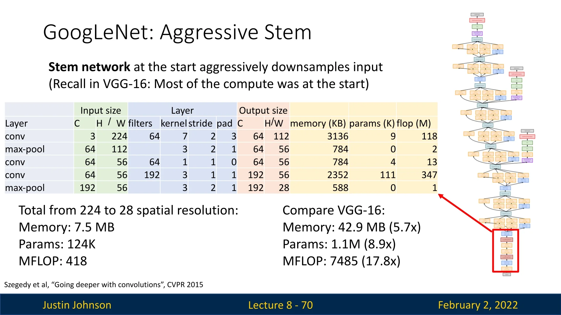
8.4.1 Stem Network: Efficient Early Downsampling

A key challenge in convolutional networks is the high computational cost at early layers, where feature maps still have large spatial dimensions. GoogLeNet tackled this by incorporating an aggressive stem network to downsample the input as early as possible.

Key properties of the stem network:

• Early Downsampling: Reduces the input resolution from \(224 \times 224\) to \(28 \times 28\) in just a few layers.
• Efficient Convolution-Pooling Sequence: Uses a combination of \(7\times 7\) and \(3\times 3\) convolutions with max pooling, minimizing computation while retaining spatial information.

• Comparison to VGG-16: The same spatial downsampling in VGG-16 is significantly more expensive:

  • Memory Usage: GoogLeNet requires only 7.5MB, whereas VGG-16 requires 42.9MB (\(5.7\times \) more).
  • Learnable Parameters: GoogLeNet has only 124k parameters, compared to VGG-16’s 1.1M (\(8.9\times \) more).
  • Computational Cost: GoogLeNet performs 418M MACs, while VGG-16 requires 7.5B MACs (\(17.8\times \) more).

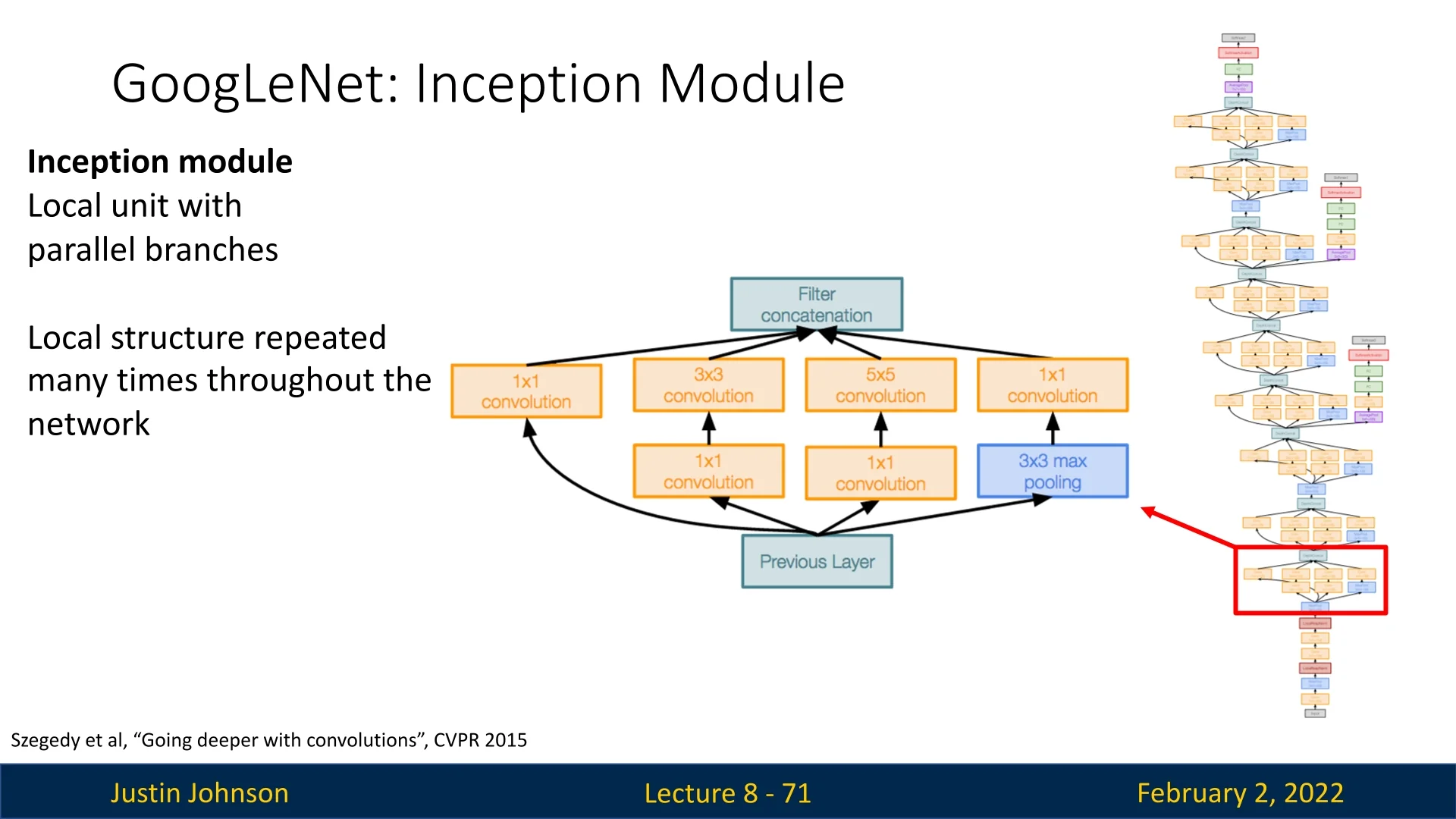
8.4.2 The Inception Module: Parallel Feature Extraction

One of the key innovations of GoogLeNet is the Inception module, a computational unit designed to process feature maps at multiple scales in parallel.

By introducing parallel branches with different receptive fields, this module enables efficient feature extraction while allowing the network to scale in depth without excessive computational overhead.

Key Advantages of the Inception Module:

• Multi-Scale Feature Extraction: Different kernel sizes capture patterns ranging from fine-grained details to high-level structures.
• Parallel Computation: Instead of stacking convolutions sequentially, multiple paths operate simultaneously, enhancing representation capacity.
• Computational Efficiency: \(1\times 1\) convolutions act as bottlenecks, reducing feature map dimensionality before expensive operations, minimizing FLOPs.
• Enhanced Gradient Flow: The presence of multiple paths mitigates the risk of vanishing gradients as it is more likely that at least some branches provide strong error signals during backpropagation.

Why Does the Inception Module Improve Gradient Flow?

Deep networks often suffer from vanishing gradients, where early layers receive increasingly weaker updates during backpropagation. The Inception module alleviates this issue through its parallel structure, which improves gradient propagation in three key ways:

• Independent Gradient Paths: Each branch processes activations separately and maintains its own set of parameters. This reduces the likelihood that all branches simultaneously produce near-zero gradients. If one path contributes weak updates, another—operating at a different scale—can still carry strong signals.

• Summation of Gradients: The outputs of all branches are concatenated before passing to the next layer. Consequently, during backpropagation, their gradient contributions are aggregated: \[ \frac {\partial L}{\partial x} = \sum _{i=1}^{k} \frac {\partial L}{\partial o_i} \frac {\partial o_i}{\partial x} \] where \( o_i \) is the output from branch \( i \), and \( x \) represents the input feature maps. Since multiple gradient paths are combined, the total error signal is less likely to diminish unless all branches saturate simultaneously.
• Redundancy and Robustness: Different branches specialize in different spatial contexts—some capturing fine textures (\(1\times 1\)), while others focus on larger structures (\(3\times 3\), \(5\times 5\)). This diversity prevents any single failure from critically weakening gradient propagation, ensuring stable training dynamics.

Structure of the Inception Module Each Inception module consists of four parallel branches, designed to extract diverse features efficiently:

• \(1\times 1\) Convolution: Reduces channel dimensions before expensive operations, improving computational efficiency while selecting relevant features.
• \(3\times 3\) Convolution: Captures mid-scale features, often preceded by a \(1\times 1\) compression layer.
• \(5\times 5\) Convolution: Extracts large-scale patterns, again typically following \(1\times 1\) convolution, acting as a feature selection mechanism, reducing the computational complexity of the convolution operation.
• Max Pooling \(+\) \(1\times 1\) Convolution: Downsamples features while preserving dominant activations, with a subsequent \(1\times 1\) layer for additional refinement.

By combining these diverse pathways, the Inception module enables deep architectures with improved gradient propagation, computational efficiency, and strong feature representation.

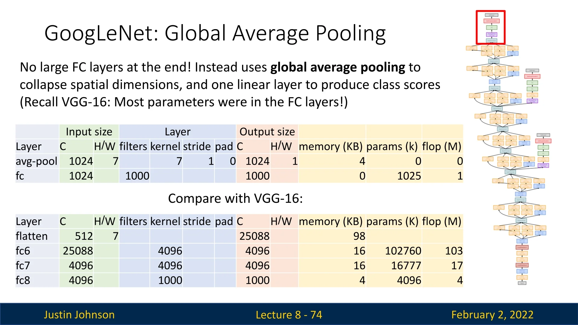
8.4.3 Global Average Pooling (GAP)

Unlike previous architectures like AlexNet and VGG, which relied on fully connected layers (MLP head) at the end, GoogLeNet introduced Global Average Pooling (GAP) as a more efficient alternative.

Key benefits:

• Parameter Reduction: VGG’s fully connected layers contained most of the network’s parameters. Replacing them with GAP dramatically reduces learnable parameters.
• Lower Computational Cost: GAP minimizes the number of floating-point operations (FLOPs), making inference faster.
• Prevents Overfitting: Large fully connected layers tend to overfit; GAP forces the network to use global spatial information instead.

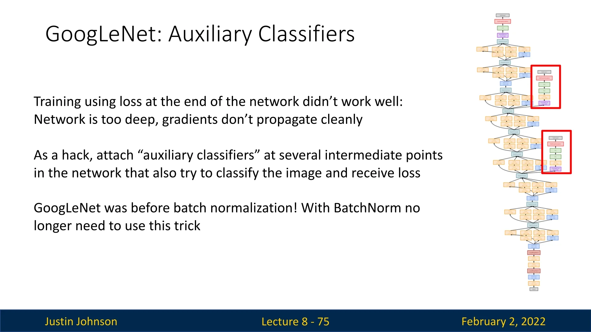
8.4.4 Auxiliary Classifiers: A Workaround for Vanishing Gradients

Before Batch Normalization (BN), training deep networks suffered from the vanishing gradient problem, where early layers received weak updates, slowing convergence. To counter this, GoogLeNet introduced Auxiliary Classifiers—intermediate classification heads that reinforced gradient signals and stabilized training. These weren’t used in the inference stage post training though, and were only introduced to enable the training of this relatively deep architecture.

Why Were Auxiliary Classifiers Needed?

• Gradient Weakening in Deep Models: As depth increased, gradients from the final classification loss diminished, making weight updates of earlier layers ineffective.
• Optimization Instability: Weak gradients led to poor convergence, requiring extensive tuning to make training work.

How Do They Help?

• Stronger Gradient Flow: Intermediate classification losses inject useful gradients into early layers, preventing stagnation.
• Implicit Regularization: Mid-layer features must be discriminative, reducing reliance on final layers.
• Faster Convergence: Reinforcing useful patterns at multiple depths speeds up learning.

Auxiliary Classifier Design Each auxiliary head mimics the final classifier but is placed at an intermediate layer:

• \(5\times 5\) average pooling (stride=3) for spatial reduction.
• \(1\times 1\) convolution (128 filters) for channel compression.
• Two fully connected layers (1024, then 1000 outputs).
• Softmax classifier.

During training, their losses contribute to the total objective (typically weighted by 0.3), ensuring they guide learning without dominating.

Gradient Flow and Regularization

• Improved Gradient Propagation:

  • Gradient Shortcuts: Auxiliary classifiers provide alternative paths for gradients, reducing their decay over depth.
  • Early Feature Learning: Mid-network supervision ensures meaningful representations emerge sooner.

• Implicit Regularization:

  • Encouraging Early Discrimination: Forces mid-level features to be useful on their own.
  • Multi-Task Effect: Training on intermediate classifications improves generalization.

Relevance Today With the introduction of Batch Normalization and Residual Connections, auxiliary classifiers have become obsolete. However, they played a crucial role in pioneering deep architectures before these stabilizing techniques were developed.

Conclusion Auxiliary classifiers were an essential workaround for training deep networks before BN. By injecting intermediate supervision, they improved gradient flow, acted as implicit regularizers, and accelerated convergence. While no longer common, they highlight the importance of effective gradient propagation in deep learning design.

8.5 The Rise of Residual Networks (ResNets)

8.5.1 Challenges in Training Deep Neural Networks

As we have seen with VGG and GoogLeNet, training deep neural networks in 2014 required numerous training tricks. Even with these techniques, increasing the network depth often led to degraded performance. However, in 2015, a breakthrough came with the introduction of Residual Networks (ResNets) by He et al. [206].

One of the key research discoveries that preceded ResNets was Batch Normalization, which we previously covered. BatchNorm allowed deeper models such as VGG and GoogLeNet to be trained without additional tricks. However, the introduction of residual connections in ResNets was another crucial innovation that enabled much deeper networks to train successfully.

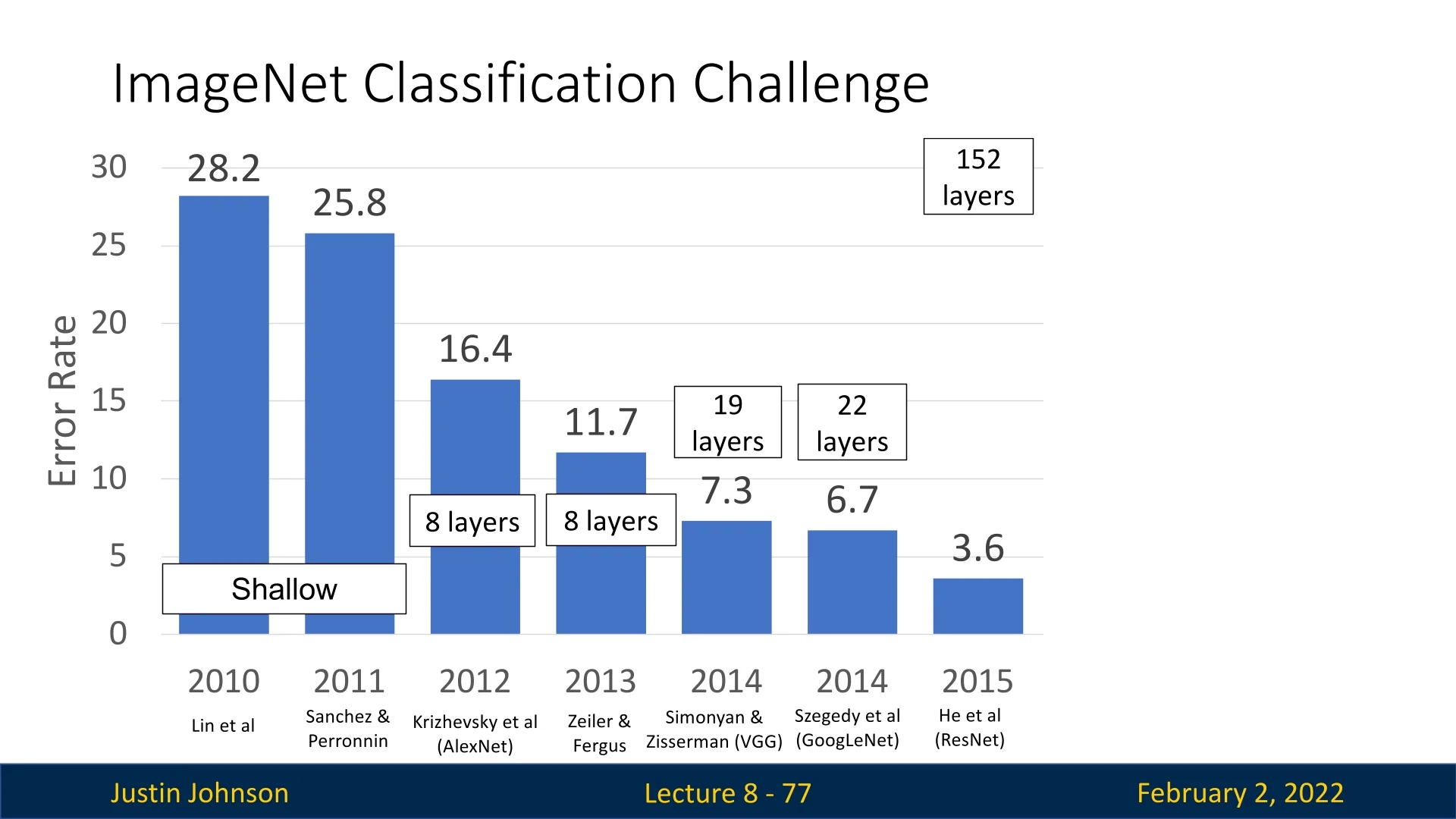
8.5.2 The Need for Residual Connections

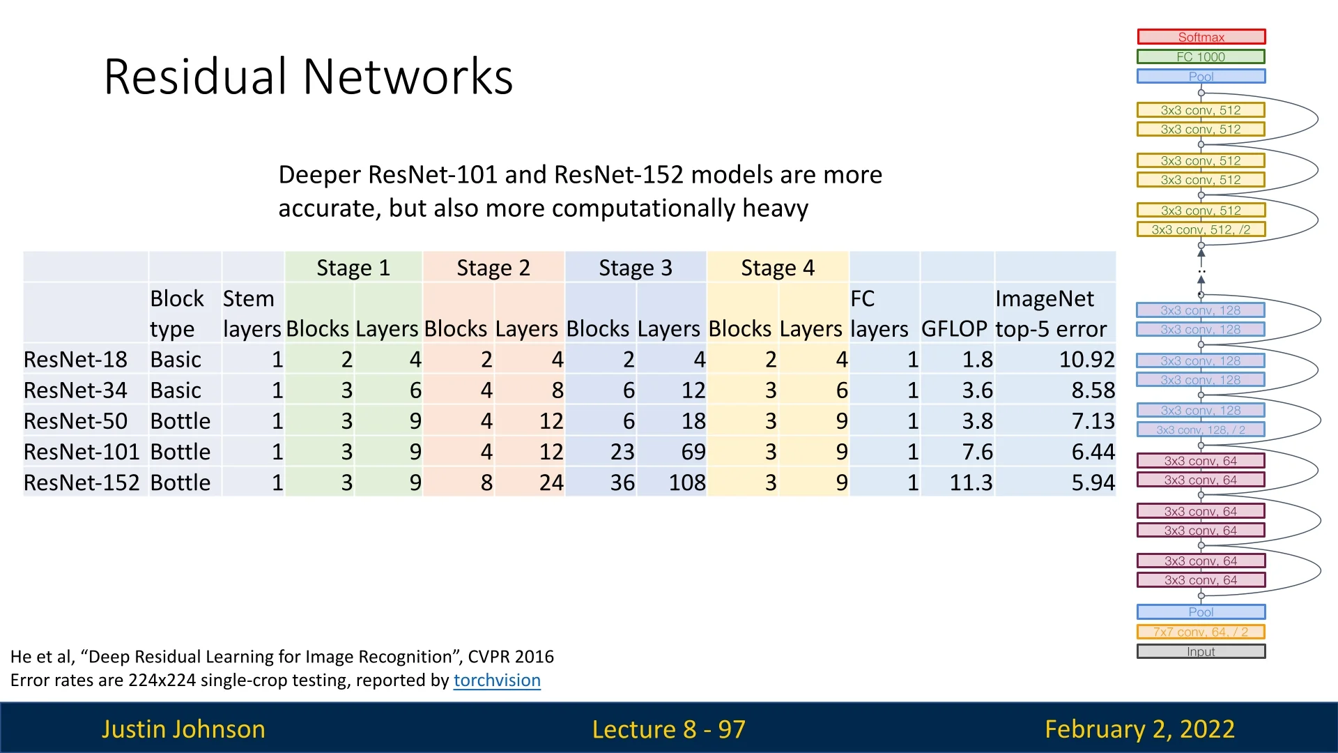
The number of layers in top-performing ImageNet models increased dramatically with ResNets, from 19 layers in VGG-19 and 22 layers in GoogLeNet to 152 layers in ResNet-152. This increase in depth was only possible due to residual connections, which allowed deeper models to be optimized effectively. The introduction of ResNets led to a significant drop in classification error rates, from 6.7% in 2014 with GoogLeNet to 3.6% with ResNets.

However, why weren’t batch normalization and other techniques sufficient? Before the introduction of residual connections, deeper models often performed worse than shallower models. Initially, researchers hypothesized that this degradation was due to overfitting. However, when examining the training performance of smaller and larger networks, they found that the deeper models were actually underfitting rather than overfitting, suggesting an optimization problem.

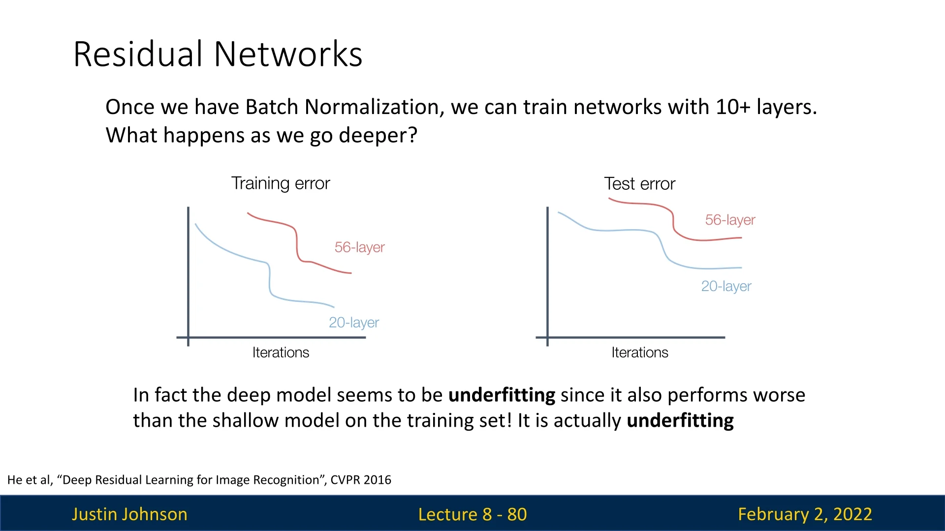
This observation was counterintuitive—deeper models should, in theory, be able to mimic shallower models by copying their layers and learning identity mappings. However, in practice, deeper models struggled to approximate the identity function where needed.

8.5.3 Introducing Residual Blocks

Deep networks often suffer from the vanishing gradient problem, making it difficult for early layers to learn meaningful features. Residual connections were introduced to alleviate this issue by reformulating the mapping that a block of layers must learn.

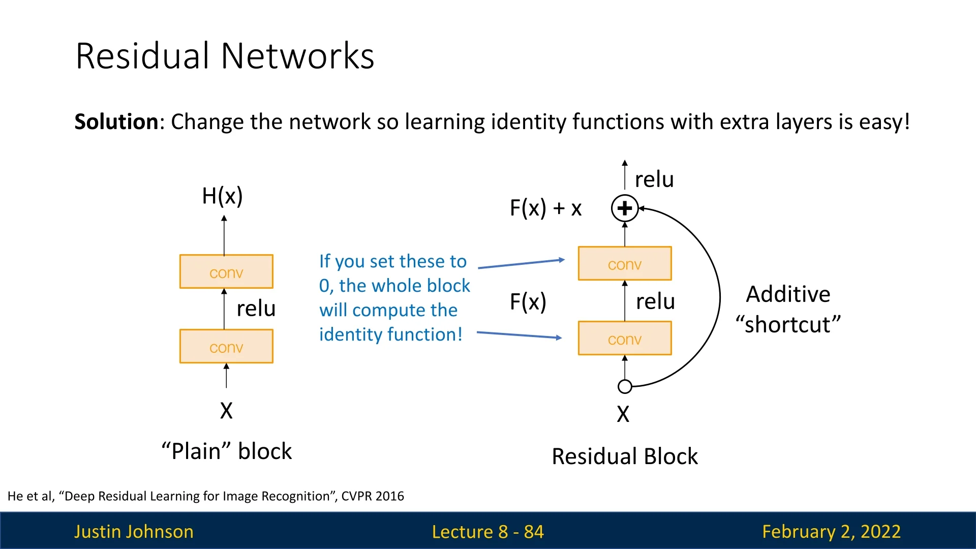
Rather than forcing layers to learn a direct mapping \(H(\mathbf {x})\), a residual block is designed to learn a residual function \(\mathcal {F}(\mathbf {x})\) such that: \[ H(\mathbf {x}) = \mathcal {F}(\mathbf {x}) + \mathbf {x}. \] Here, \(\mathbf {x}\) is the input to the block and \(\mathcal {F}(\mathbf {x})\) is typically the output of a series of convolutional layers. The shortcut connection directly adds \(\mathbf {x}\) to the output of the residual branch.

Intuition Behind Residual Connections

• Easier Learning of the Identity: If the optimal transformation is close to the identity, the residual branch can learn to output zeros, so that the block’s overall function is nearly \(\mathbf {x}\). This makes it much easier to train very deep networks.The shortcut thus provides an alternate path for the gradient to flow directly from later layers to earlier ones.
• Flexible Feature Refinement: Even if the residual branch is not perfectly optimized, the network can still rely on the shortcut to preserve useful information. The extra non-linearity introduced in the residual branch adds expressiveness without forcing the entire block to deviate dramatically from the identity.

By enabling layers to essentially “skip” learning complex transformations when unnecessary, residual blocks allow very deep networks to be trained more efficiently and reliably.

8.5.4 Architectural Design of ResNets

ResNets combine the best aspects of both VGG and GoogLeNet:

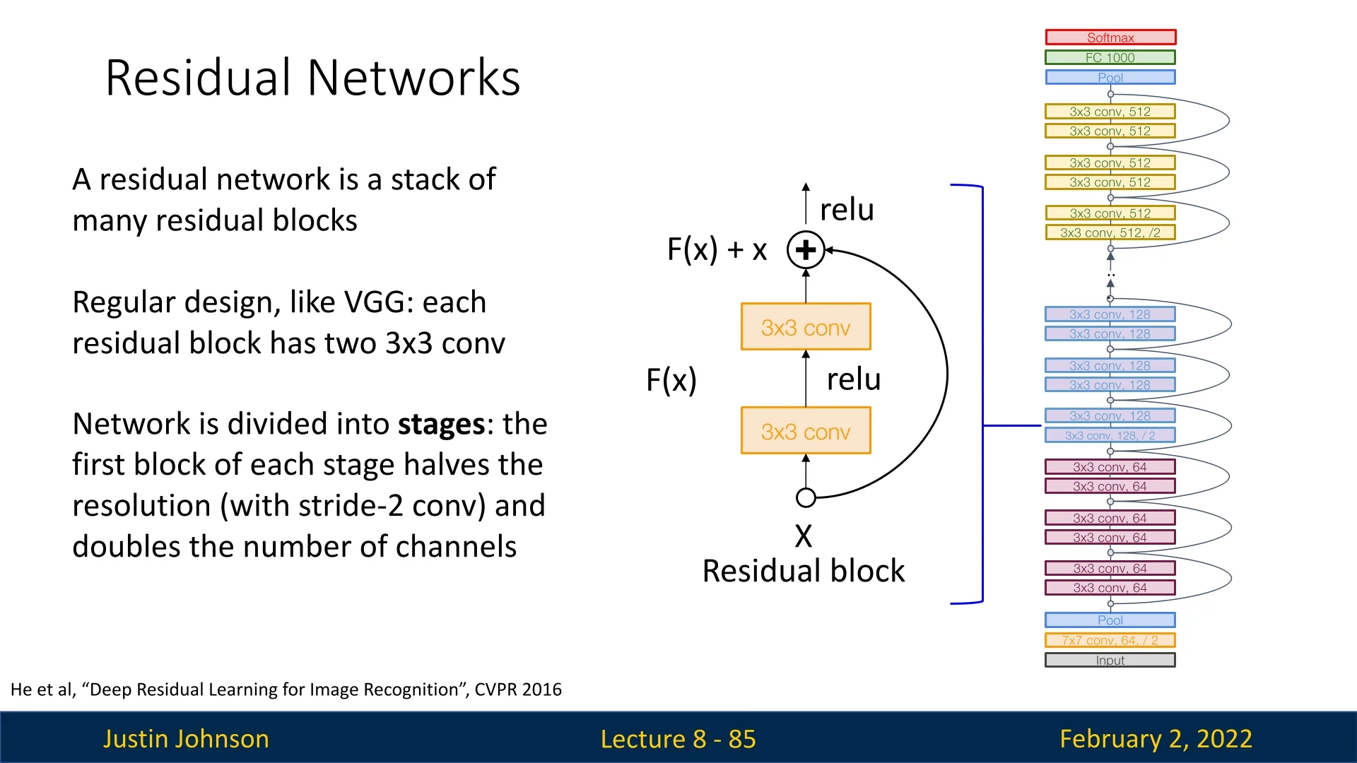
• VGG-style regularity: ResNets are structured into stages, where each residual block consists of two 3x3 convolutional layers.
• Stage-wise downsampling: The first block in each stage reduces the spatial resolution (via stride-2 convolutions) while doubling the number of channels, like in VGG.
• GoogLeNet-inspired efficiency: ResNets incorporate a stem network at the beginning and use global average pooling at the end, eliminating fully connected layers.

8.5.5 Bottleneck Blocks for Deeper Networks

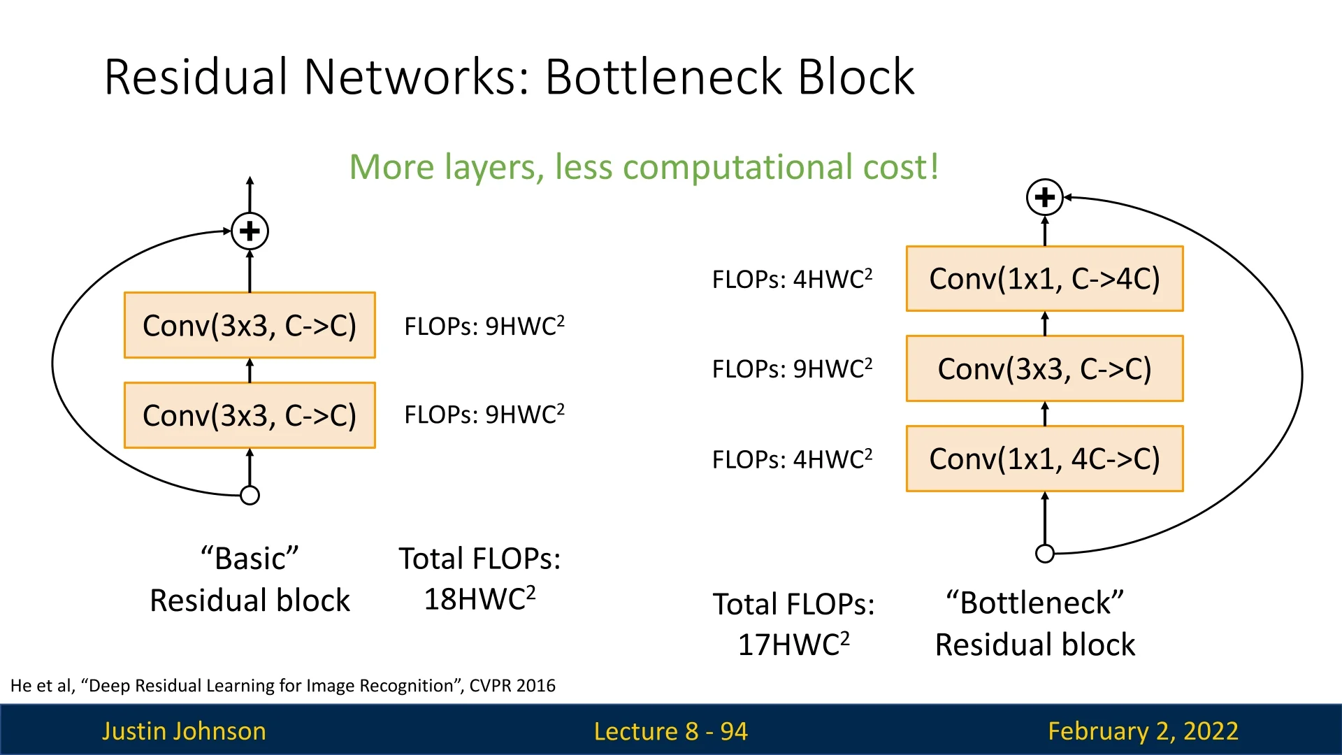
ResNets also introduced an improved residual block design called the bottleneck block, inspired by GoogLeNet’s inception module. Instead of using two 3x3 convolutions per block, the bottleneck block includes:

• A \( 1 \times 1 \) convolution to reduce dimensionality (\( 4C \to C \))
• A \( 3 \times 3 \) convolution for feature extraction (\( C \to C \))
• A \( 1 \times 1 \) convolution to restore dimensionality (\( C \to 4C \))

This change enables deeper networks with slightly reduced computational costs.

8.5.6 ResNet Winning Streak and Continued Influence

The introduction of ResNets in 2015 revolutionized deep learning, particularly in the ImageNet Large Scale Visual Recognition Challenge (ILSVRC). ResNets dominated the competition, securing first place in all five main tracks, including image classification, object detection, and segmentation. Their ability to scale to depths previously considered untrainable led to a significant reduction in classification error rates, with ResNet-152 achieving a top-5 error rate of just 3.6%, far outperforming previous state-of-the-art architectures.

Beyond ImageNet, ResNets proved highly effective in broader computer vision tasks. They became a fundamental backbone for models tackling object detection and segmentation, leading to state-of-the-art performance on the COCO (Common Objects in Context) dataset [358]. COCO is a large-scale dataset designed for object detection, segmentation, and captioning, featuring over 200,000 labeled images across 80 object categories. The dataset’s diversity and complexity make it a critical benchmark for evaluating model generalization beyond classification.

ResNets’ impact extended to COCO challenges, where they enabled significant improvements in object detection frameworks such as Faster R-CNN and Mask R-CNN (which we’ll cover extensively later). Their superior feature extraction capabilities provided more robust representations, leading to more precise bounding box localization and segmentation masks. These results solidified ResNets as the dominant architecture for both classification and detection tasks, influencing deep learning research for years to come.

Even today, ResNets remain a cornerstone of deep learning. Variants like ResNeXt, Wide ResNets, and ResNet-D have refined the architecture further, while modern Transformer-based vision models still incorporate residual connections inspired by ResNets’ fundamental design.

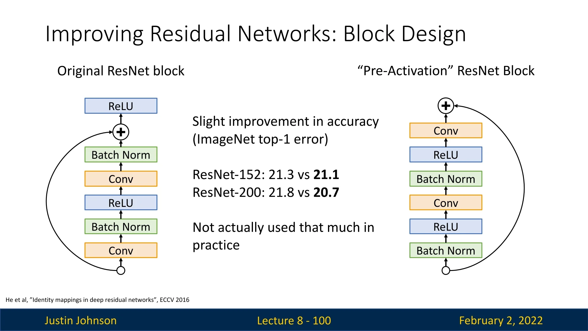
8.5.7 Further Improvements: Pre-Activation Blocks

A later study found that switching the order of operations within residual blocks—from Conv-BN-ReLU to BN-ReLU-Conv—further improved accuracy. These pre-activation blocks help refine gradient flow and boost network performance [208].

8.5.8 Architectural Comparisons and Evolution Beyond ResNet

The 2016 ImageNet Challenge: Lack of Novelty

The 2016 ImageNet competition saw no major architectural breakthroughs. Instead, the winning team employed an ensemble of multiple models, leveraging the strengths of different architectures to achieve superior accuracy. While effective in practice, this approach did not introduce fundamental innovations or new design principles for deep networks.

Comparing Model Complexity and Efficiency

By 2017, several architectures had competed for dominance in computer vision, each offering a trade-off between accuracy, computational cost, and memory efficiency.

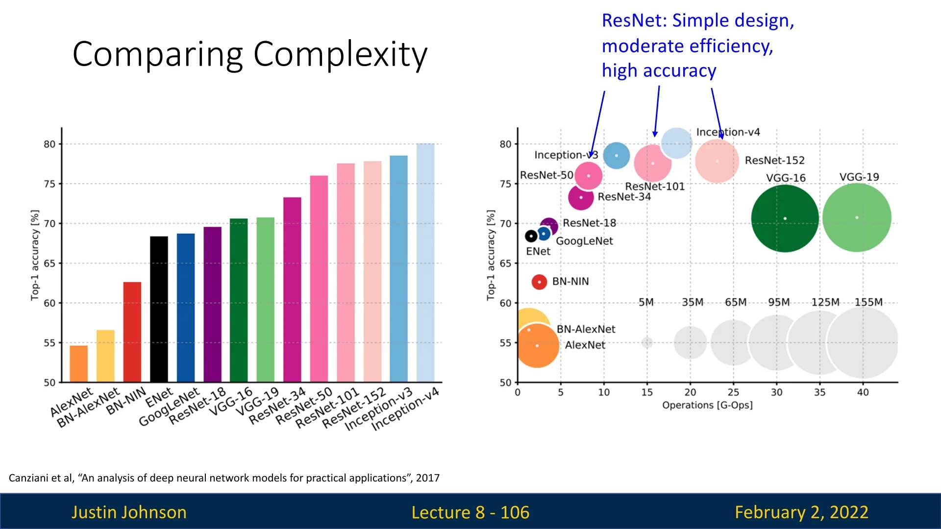
Figure 8.18 provides a comparative analysis of top-performing models across these dimensions. Key observations from this comparison:

• Inception Models: Google’s Inception series, culminating in Inception-v4 (2017), consistently achieved top-tier accuracy. However, these models were computationally expensive and had a high memory footprint due to their complex multi-branch structures.
• VGG Networks: Although instrumental in the transition to deeper CNNs, VGG models were no longer competitive in accuracy and remained highly inefficient in both computation and memory usage.
• GoogLeNet (Inception-v1): Despite being more parameter-efficient than VGG, GoogLeNet did not perform as well as the best models in terms of accuracy.
• AlexNet: The first breakthrough deep CNN in 2012, AlexNet was now vastly outperformed by newer architectures. While it had many learnable parameters, it was not computationally expensive but significantly lagged in accuracy.
• ResNets: Residual Networks remained among the top architectures, striking a balance between accuracy, simplicity, and efficiency. They provided strong generalization with moderate computational demands compared to Inception-based models.

Beyond ResNets: Refinements and Lightweight Models

While ResNets set a new standard for deep learning architectures, further refinements and specialized models emerged in later years. Some notable advancements include:

• ResNeXt: A modular extension of ResNet, ResNeXt introduced a grouped convolution strategy, inspired by Inception’s parallel paths, achieving better accuracy without significantly increasing computational cost.
• MobileNets and ShuffleNets: Recognizing the need for efficient models suitable for edge devices, researchers developed lightweight architectures such as MobileNets and ShuffleNets. These models used depthwise separable convolutions and grouped convolutions to reduce computational complexity while maintaining competitive performance. We will cover these extensively in later sections.

The landscape of CNN architectures continued evolving post-ResNets, with a focus on improving computational efficiency and extending deep learning capabilities beyond high-performance GPUs to mobile and embedded platforms.