Lecture 24: Videos (Video Understanding)
24.1 Introduction to Video Understanding
Up to this point, our discussion has focused mainly on images, typically represented as 3D tensors of shape \(C \times H \times W\), where \(C\) denotes the number of channels (often three for RGB). In this chapter we generalize from static images to videos, which can be viewed as sequences of images indexed by time. A video is therefore represented by a 4D tensor of shape: \begin {equation} \label {eq:chapter24_video_tensor} \mathbf {V} \in \mathbb {R}^{T \times C \times H \times W}, \end {equation} where \(T\) denotes the temporal dimension, corresponding to the number of frames in the sequence.
This extension introduces a fundamental challenge: while image analysis largely emphasizes spatial patterns, video understanding requires us to jointly reason about spatial and temporal structures. Tasks defined over videos range widely, from video classification and temporal action localization to video captioning and generation. In this lecture and chapter we focus on video understanding, that is, building models that interpret the content of a video clip to predict semantic properties such as actions, interactions, or events.
24.1.1 From Images to Videos
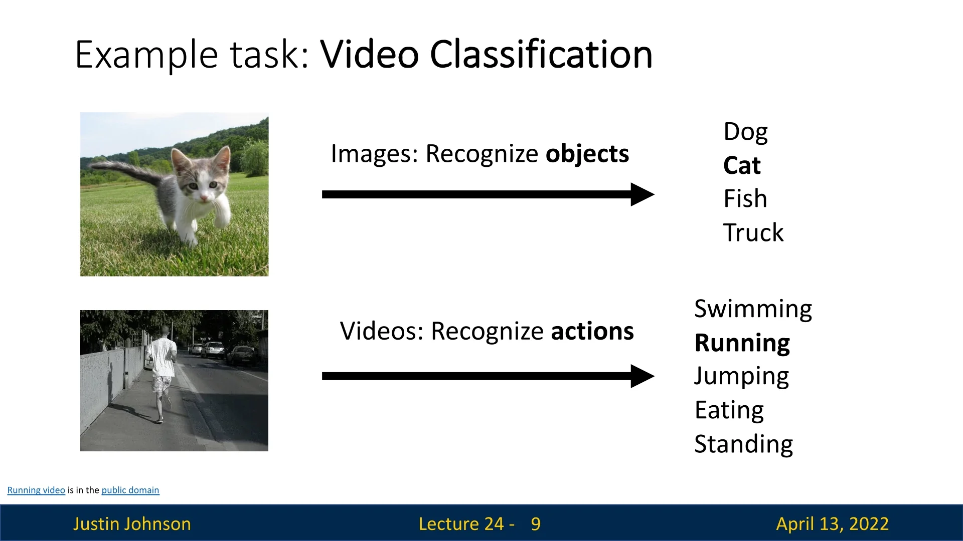
In image classification, the objective is typically to detect the presence of objects (e.g., predicting that an image contains a cat). In contrast, video classification aims to recognize actions. For example, given a short clip of a person, the model should distinguish whether the individual is running, walking, jumping, or standing. This shift from nouns (objects) to verbs (actions) reflects the additional temporal complexity inherent in videos.
24.1.2 Challenges of Video Data and Clip-Based Training
Videos present substantial computational burdens compared to images. A standard video stream is recorded at approximately 30 frames per second, with each frame containing hundreds of thousands or millions of pixels. For example, storing an uncompressed video requires approximately:
- \(\sim \)1.5 GB per minute for standard definition (640 \(\times \) 480),
- \(\sim \)10 GB per minute for high definition (1920 \(\times \) 1080).
This scale makes it infeasible to directly train on raw, full-length videos.
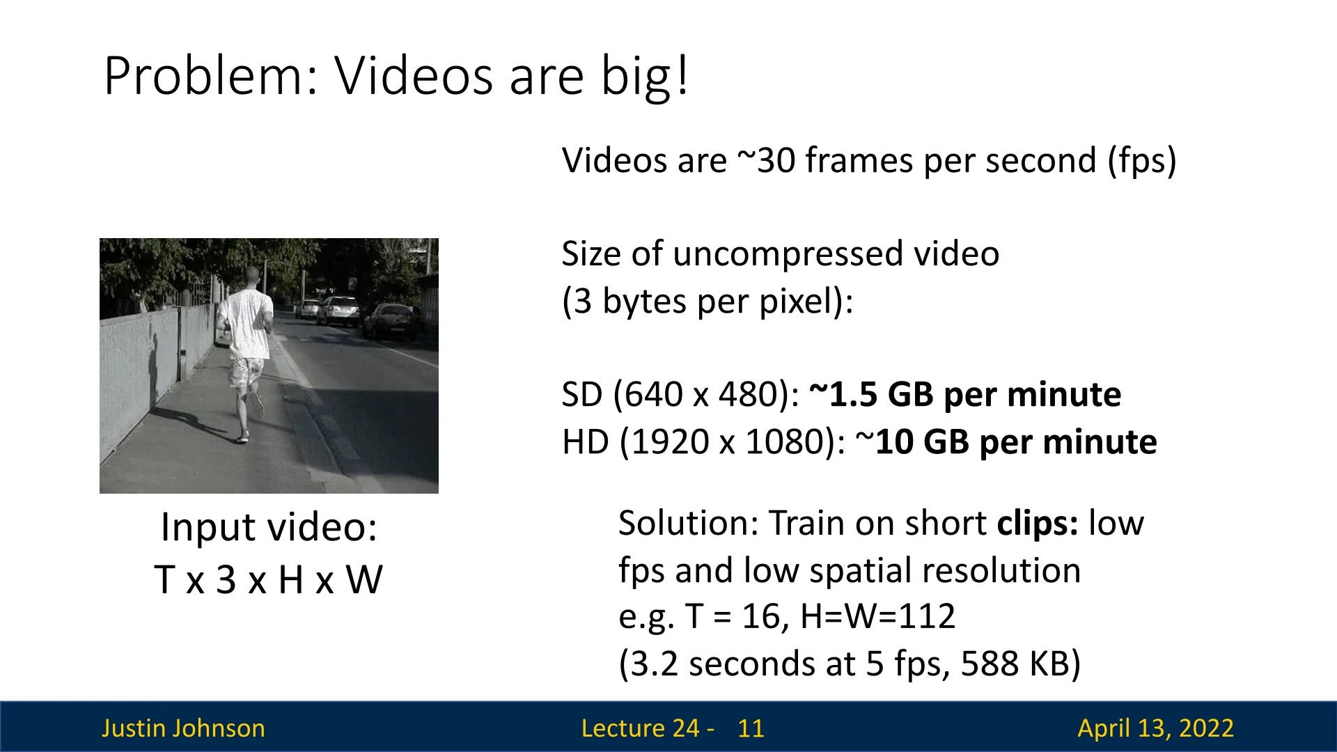
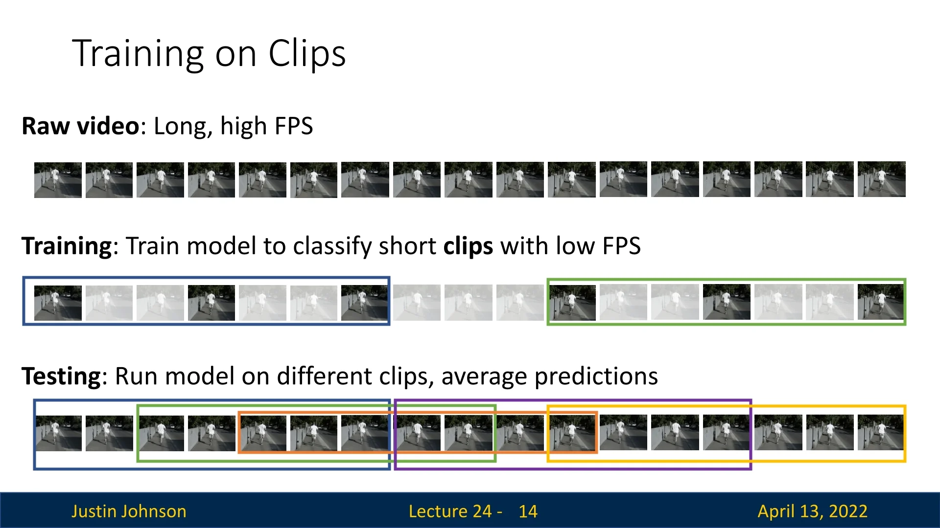
The standard solution is to train on short clips rather than entire videos. A raw sequence of length \(T_\mbox{raw}\) is divided into windows of \(T\) consecutive frames, often subsampled in time (e.g., taking every \(k\)th frame) to reduce the effective frame rate. Clips are also downsampled spatially (e.g., \(112 \times 112\) pixels). During training, models are supervised on these short clips.
At test time, multiple clips are sampled from different temporal regions of the video. The model processes each subclip independently, and the results are aggregated—typically via averaging—to produce a robust video-level prediction.
24.2 Video Classification as a Canonical Task
Video classification serves as a canonical entry point into video understanding. The task is defined as mapping an input clip \(\mathbf {V} \in \mathbb {R}^{T \times C \times H \times W}\) to a label \(y \in \{1,\dots ,K\}\) from a fixed action vocabulary of size \(K\). Formally, we seek to learn a function \begin {equation} \label {eq:chapter24_video_classification} f_\theta : \mathbb {R}^{T \times C \times H \times W} \to \{1,\dots ,K\}, \end {equation} where \(\theta \) denotes the parameters of the model. As in image classification, the system is typically trained with cross-entropy loss. However, the network architecture must incorporate temporal reasoning, either explicitly or implicitly, in order to succeed.
This formulation establishes video classification as a foundation for more advanced video understanding tasks, such as temporal action localization (detecting when an action occurs within an untrimmed video) and spatio-temporal action detection (localizing actions in both space and time). In the following parts, we progressively build models to handle the spatio-temporal complexity of videos, beginning with simple baselines and gradually extending to sophisticated architectures.
24.2.1 Single-Frame Baseline
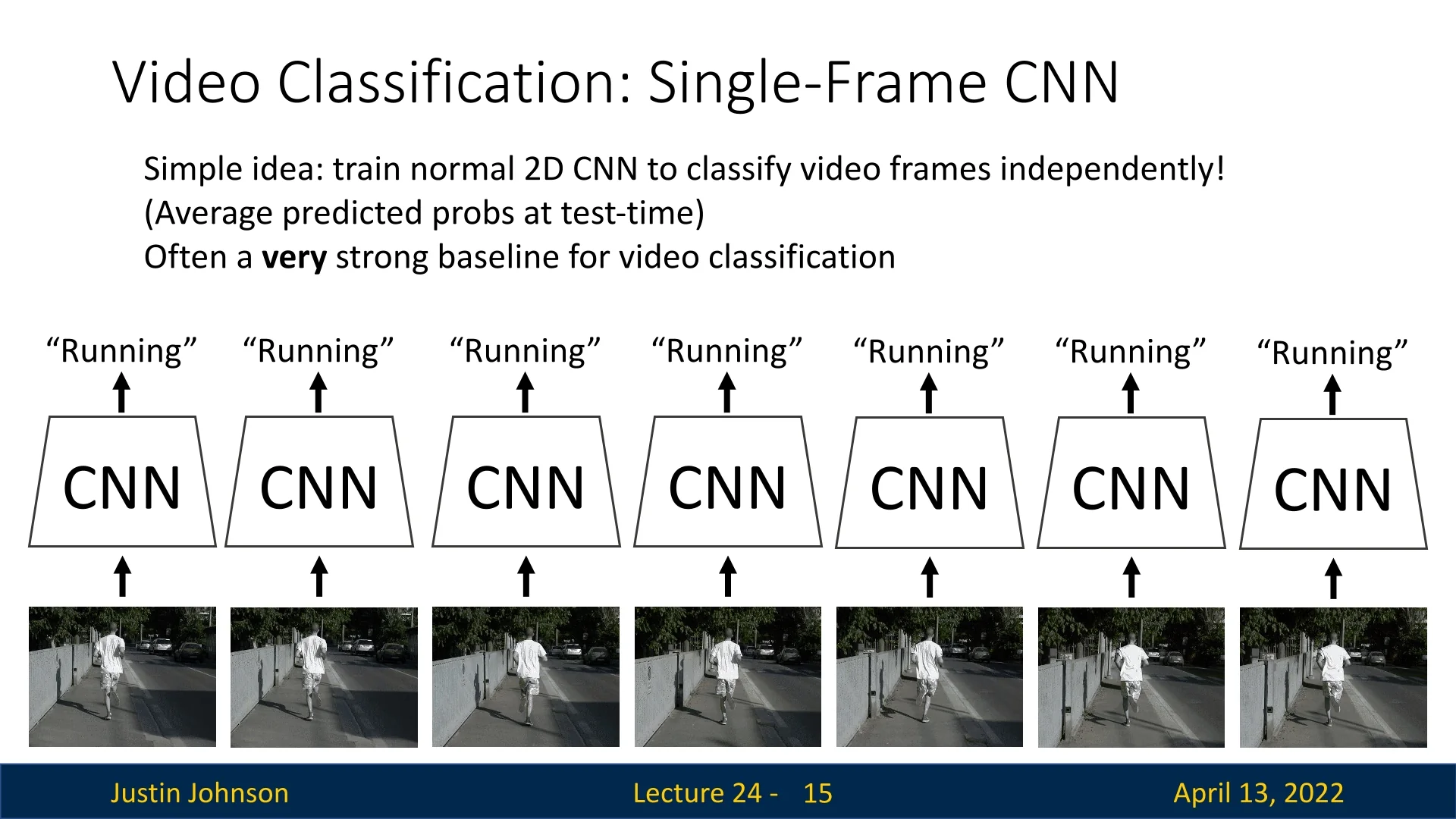
An unexpectedly strong baseline for video classification is to ignore temporal information entirely. In this approach, each frame is classified independently using a standard 2D CNN trained on individual RGB frames with the video-level label. At test time, predictions across frames are averaged to obtain the final decision. While simple, this baseline often achieves competitive accuracy and should always be attempted first in practice.
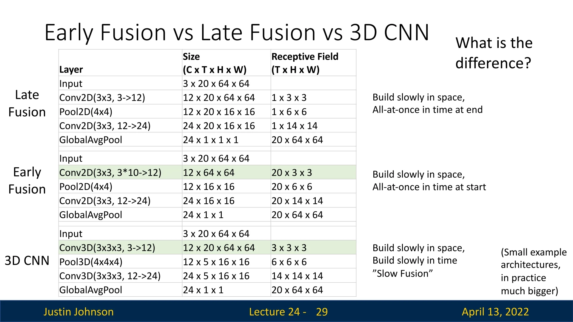
24.2.2 Late Fusion
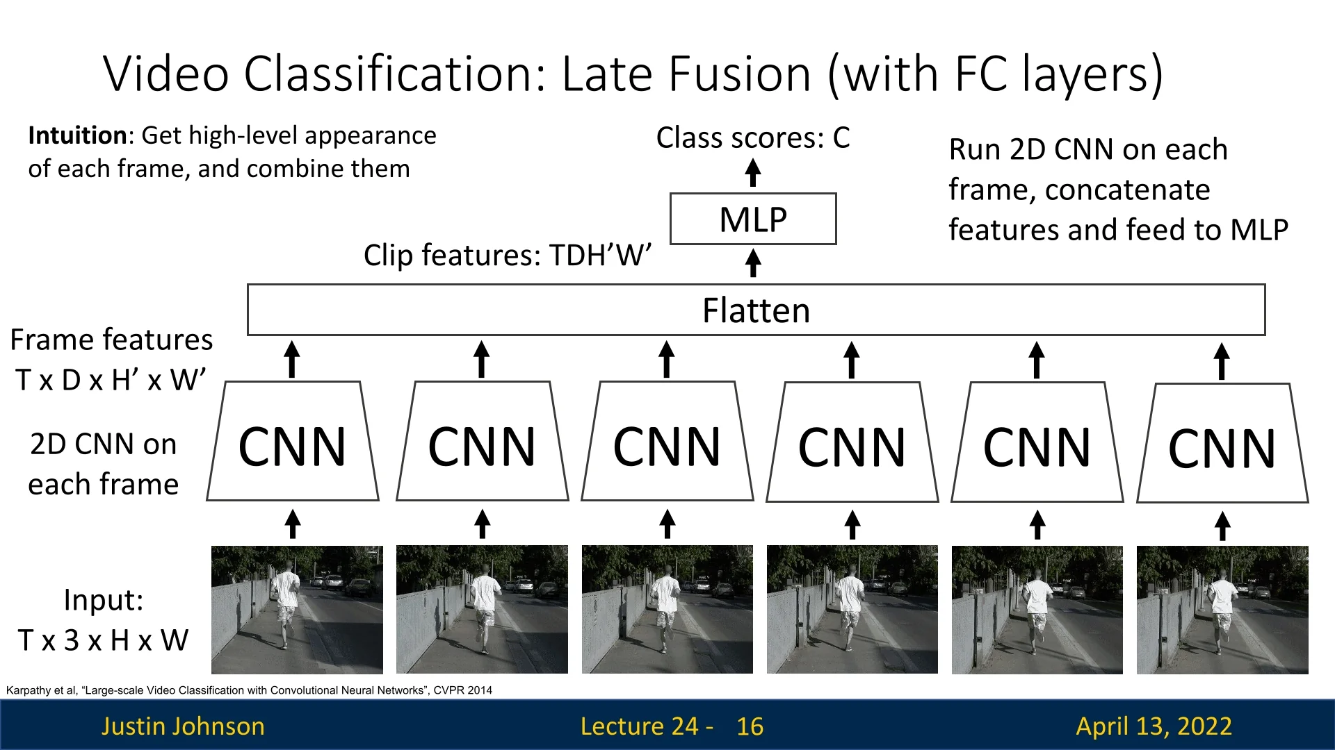
To incorporate temporal reasoning, a natural extension is late fusion. Here, each frame is first processed independently by a 2D CNN to produce feature maps of shape \(D \times H' \times W'\). The sequence of features across \(T\) frames is then concatenated into a tensor of shape \(T \times D \times H' \times W'\). This can be flattened into a single feature vector of dimension \(TDH'W'\), followed by fully connected layers and a softmax classifier: \begin {equation} \label {eq:chapter24_late_fusion} \hat {y} = \mbox{Softmax}\big ( \mbox{MLP}(\mbox{Flatten}(\{f_1,\dots ,f_T\})) \big ), \end {equation} where \(f_t\) denotes the per-frame CNN features.
The intuition is that we first capture high-level appearance in each frame and then combine them at the classification stage.
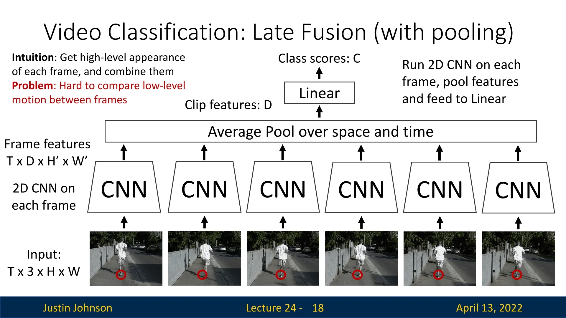
A more parameter-efficient variant replaces the flatten–FC stage with global average pooling (GAP) over both spatial and temporal dimensions, yielding a compact \(D\)-dimensional vector before the classifier. While effective at reducing overfitting, late fusion methods have a key limitation: they struggle to capture fine-grained motion signals between consecutive frames, since temporal information is collapsed only at a late stage.
24.2.3 Early Fusion
To better model small/fine-grained temporal dynamics, we can adopt early fusion. Here, the temporal dimension is reshaped into the channel dimension: the input clip \(\mathbb {R}^{T \times 3 \times H \times W}\) is reformatted into \(\mathbb {R}^{3T \times H \times W}\). A 2D CNN is then applied, treating time-stacked frames as an enlarged channel input. This allows the first convolutional layer to directly compare pixel intensities across adjacent frames, thereby capturing short-term motion.
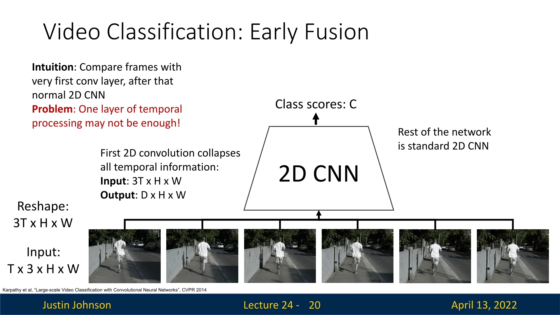
While this mitigates late fusion’s inability to capture motion, the temporal dimension is collapsed after the first convolution. This one-shot fusion can be overly aggressive, discarding longer-range temporal information, and thus harm classification results.
24.2.4 3D CNNs: Slow Fusion
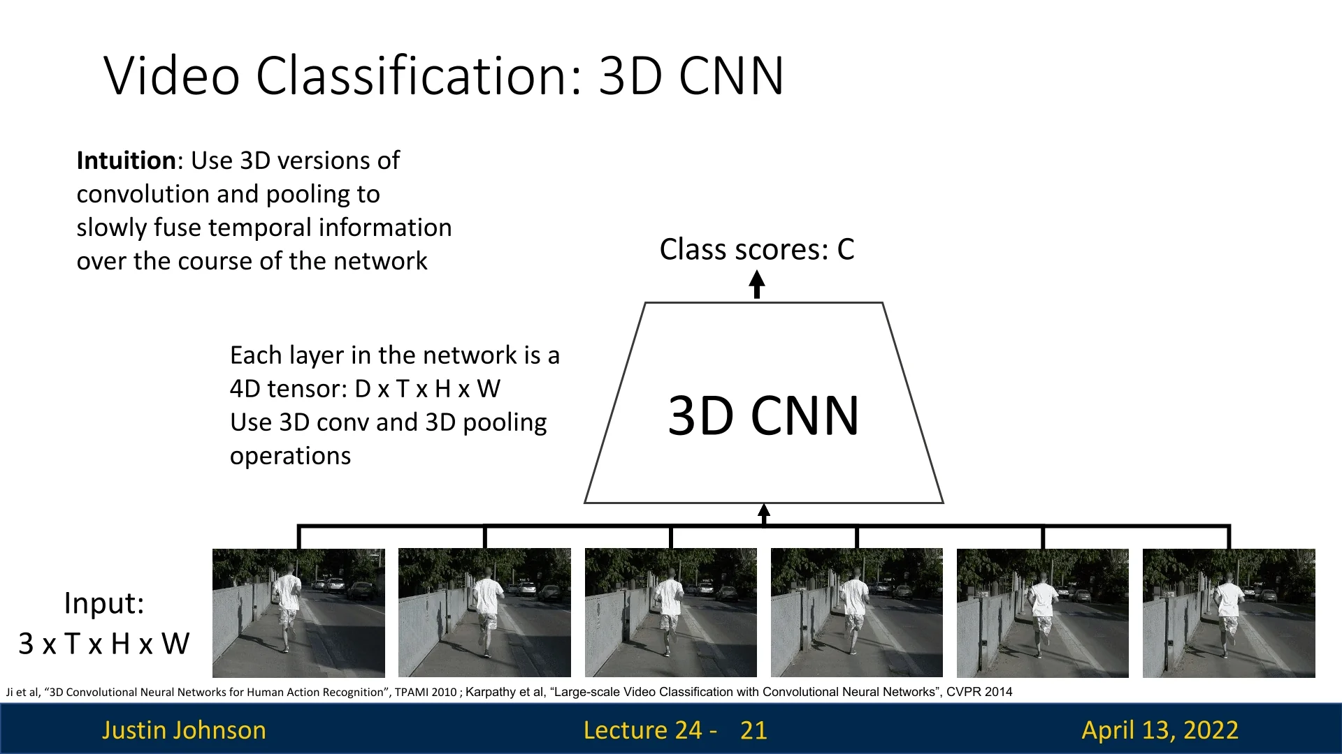
A natural extension of 2D convolution to video is to treat time as an additional dimension and apply 3D convolutions. In this design, filters have shape \(K_t \times K_h \times K_w\), spanning the temporal axis as well as the spatial axes. Activations remain four-dimensional (\(D \times T \times H \times W\)), where \(T\) denotes temporal extent. By stacking such layers, temporal information is fused progressively across depth—an approach known as slow fusion.
This architecture enables hierarchical learning of spatiotemporal features: early layers may detect short-term motion edges, while deeper layers aggregate evidence for longer-term dynamics. The formulation was pioneered in early works such as [274, 287].
Comparison with fusion alternatives. To place 3D CNNs in context, it is helpful to compare with early and late fusion strategies. In early fusion, temporal information is aggregated at the input by stacking frames as channels, while spatial receptive fields grow across depth. In late fusion, each frame is processed independently by 2D CNNs, and temporal integration occurs only at the final stage. By contrast, 3D CNNs (slow fusion) expand both spatial and temporal receptive fields gradually, balancing spatial and temporal modeling capacity.
24.2.5 2D vs 3D Convolutions
To better understand the distinction between early fusion with 2D convolutions and true 3D convolutions, it is useful to analyze how their filters operate over time:
-
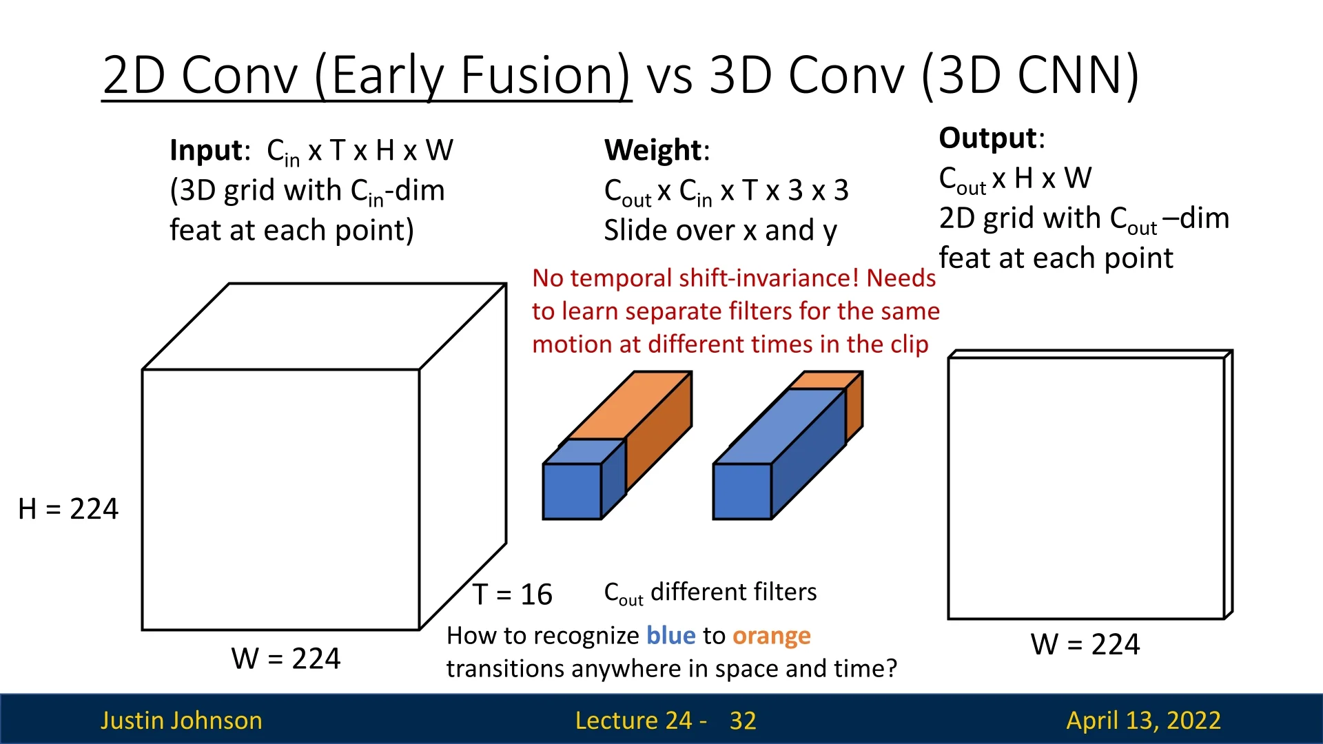
Early fusion (2D convolutions on stacked frames): Frames are concatenated along the channel dimension and processed by a 2D convolution. First-layer filters therefore have shape \[ C_\mbox{out} \times C_\mbox{in} \times T \times K_h \times K_w. \] Each filter spans the entire temporal extent \(T\). This design has two drawbacks:
- 1.
- No temporal shift invariance: the filter is tied to specific time positions. For example, a filter trained to detect a hand moving to the right between frames 1 and 2 will not automatically generalize to the same motion between frames 3 and 4. A separate set of weights must be learned for each timing.
- 2.
- Parameter inefficiency: since temporal variation must be explicitly memorized at different offsets, many more filters are needed to cover the same set of motions. This makes early fusion prone to overfitting and less data-efficient.
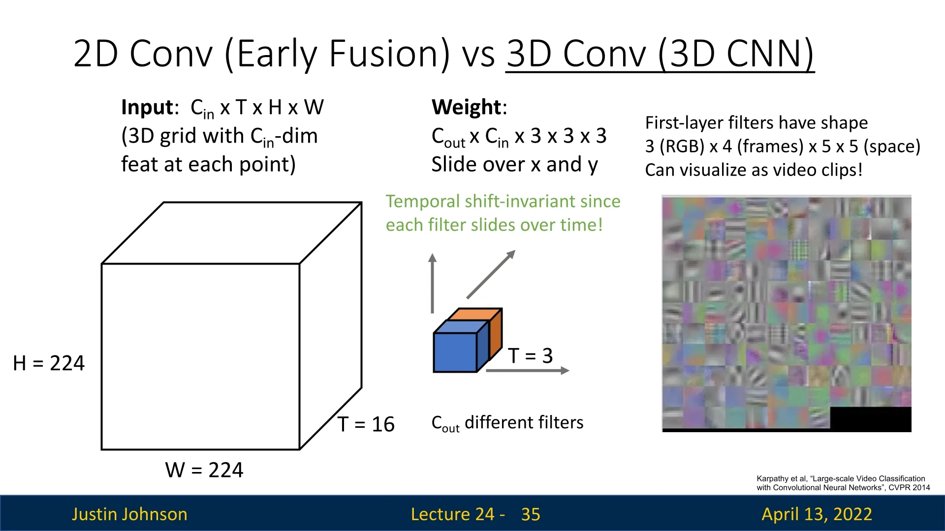
- 3D convolution (true spatiotemporal kernels): Filters extend over a limited temporal window \(K_t \ll T\), with shape \[ C_\mbox{out} \times C_\mbox{in} \times K_t \times K_h \times K_w. \] These filters slide along the temporal axis, just as 2D filters slide spatially. This provides temporal shift invariance: once a kernel has learned to detect a short motion pattern (e.g., a flick or edge moving across frames), it will activate regardless of where in the sequence that motion occurs. This is analogous to translation invariance in images, but extended into the time dimension.
For visual clarity, Justin Johnson illustrates these concepts with concrete examples. Early fusion requires separate filters to detect the same phenomenon (in the example, color transition from orange\(\!\to \!\)blue) at different times in the sequence, whereas 3D convolution achieves this with a single filter that generalizes across temporal positions.
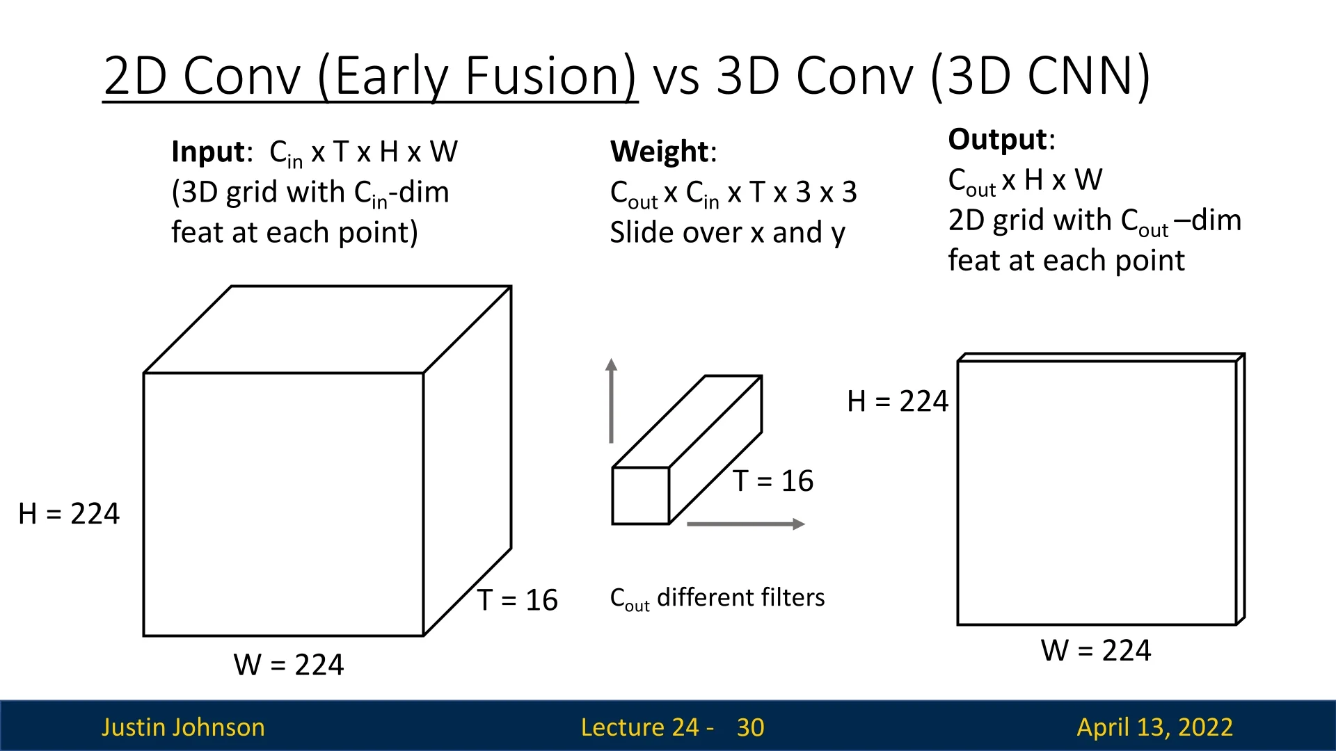
Clarifying Input Channels vs Temporal Dimension Convolutions always combine all input channels (\(C_\mbox{in}\), e.g. RGB) at once. The real difference between 2D and 3D convolutions is whether the temporal axis is collapsed or preserved, which changes the filter shape and what it can learn.
- 2D convolution (early fusion): Input: \((C_\mbox{in}\!\cdot \!T) \times H \times W\). Filter: \(C_\mbox{out} \times (C_\mbox{in}\!\cdot \!T) \times K_h \times K_w\). The filter is 2D in space (\(K_h \times K_w\)), but its depth spans all channels, including stacked frames. Thus, time is baked into channels. The network sees all frames at once but cannot reuse the same filter across time; it must learn separate filters for motion at different temporal positions.
- 3D convolution: Input: \(C_\mbox{in} \times T \times H \times W\). Filter: \(C_\mbox{out} \times C_\mbox{in} \times K_t \times K_h \times K_w\). The filter is volumetric: it spans \(K_t\) consecutive frames as well as \(K_h \times K_w\) spatial pixels. Crucially, it slides across time, height, and width. This preserves temporal structure and gives temporal shift invariance: the same filter can detect a motion pattern (e.g., a color change or edge movement) regardless of when it occurs in the sequence.
Practical implication. In early fusion (2D), the model treats the clip like a single thick image: temporal order is fixed, and motion is hard to generalize. In 3D convolution, the model treats the clip as a video volume: filters move through time as well as space, making them natural motion detectors.
24.2.6 Sports-1M Dataset and Baseline Comparisons
An influential benchmark for video classification is the Sports-1M dataset [287]. It consists of roughly one million YouTube videos labeled across 487 sports categories, ranging from common activities like basketball or soccer to highly fine-grained distinctions such as ultramarathon versus half marathon. The dataset poses unique challenges, as models must not only recognize broad classes of motion but also discriminate subtle variations within closely related activities.
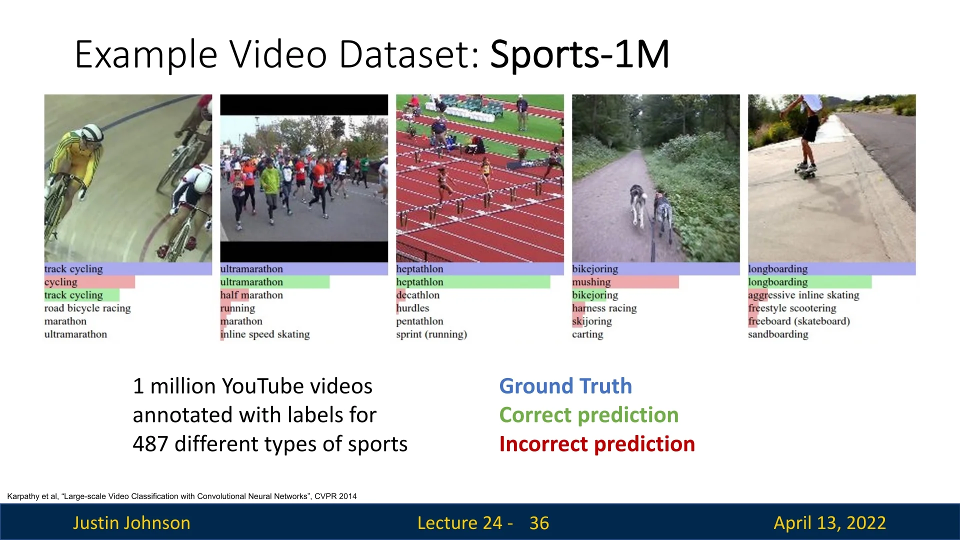
These examples illustrate the dataset’s difficulty: coarse categories are often recognized correctly, but small variations in equipment, environment, or motion patterns can determine the correct label. As a result, fine-grained sports categories highlight the challenge of models trained on video data.
24.2.7 Baseline Model Performance
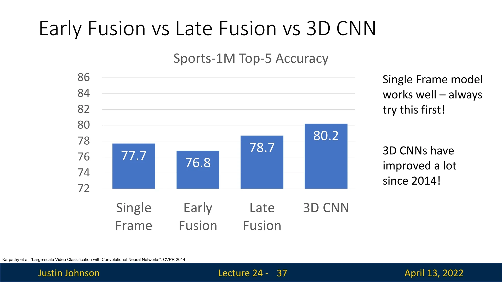
Karpathy et al. [287] benchmarked several architectures on Sports-1M, comparing single-frame CNNs, early fusion, late fusion, and 3D CNNs (slow fusion). Surprisingly, the single-frame baseline outperformed early fusion, achieving \(77.7\%\) accuracy compared to \(76.8\%\). Late fusion and 3D CNNs provided modest improvements, with \(78.7\%\) and \(80.2\%\) respectively.
These results underscore two key insights:
- 1.
- Single-frame models are strong baselines: even ignoring temporal structure, per-frame CNNs achieve competitive accuracy, making them a practical first step for many applications.
- 2.
- Temporal models offer incremental gains: incorporating temporal reasoning via late fusion or 3D CNNs provides improvements, but the gap is smaller than might be expected.
It is important to note that these experiments date back to 2014, when training resources and architectures were limited (many models were trained on CPU clusters). Since then, 3D CNN architectures and large-scale training pipelines have advanced significantly, so the reported numbers should be interpreted with caution.
24.2.8 C3D: The VGG of 3D CNNs
A landmark architecture in early video understanding was the C3D network [651], often described as “the VGG of 3D CNNs”. Recall that VGG for images was built entirely from \(3 \times 3\) convolutions and \(2 \times 2\) poolings in a simple conv–conv–pool pattern. C3D extended this idea to videos: it used \(3 \times 3 \times 3\) convolutions and \(2 \times 2 \times 2\) poolings throughout, except in the first pooling layer, which used \(1 \times 2 \times 2\) to avoid collapsing the temporal dimension too early.
This design made C3D a straightforward 3D analog of VGG and an influential baseline in the field. Importantly, the authors released pretrained weights on Sports-1M, and many subsequent works used C3D as a fixed video feature extractor.
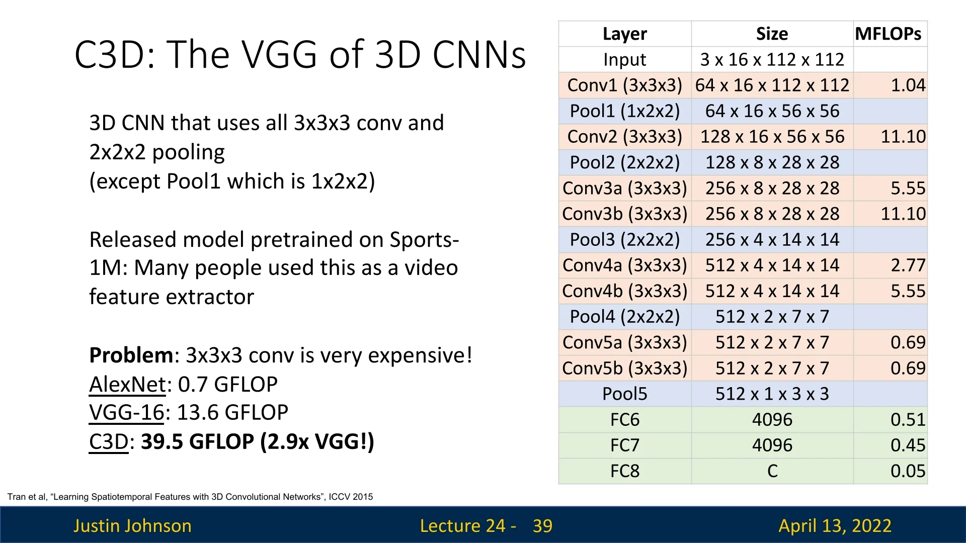
Computation cost The main drawback of C3D is its cost. Even with small inputs (16 frames of size \(112 \times 112\)), a single forward pass requires nearly 40 GFLOPs:
- AlexNet: \(0.7\) GFLOPs
- VGG-16: \(13.6\) GFLOPs
- C3D: \(39.5\) GFLOPs
This stems from sliding 3D kernels over the entire spatiotemporal volume, which scales cubically in kernel size.
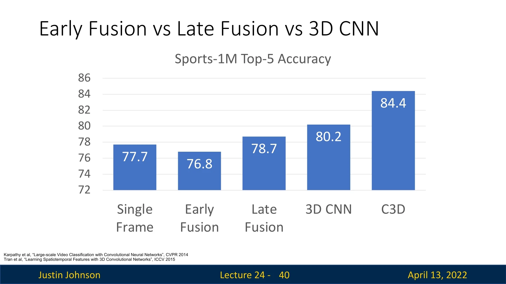
Summary The story of C3D parallels that of image models: accuracy improved by scaling up deeper, more expensive networks. But these architectures also highlighted the need to treat time and space differently, rather than as fully interchangeable.
24.3 Separating Time and Space in 3D Processing
Humans are capable of recognizing actions from motion cues alone. For example, point-light displays of moving dots are sufficient for us to perceive walking, running, or waving. This suggests that the brain processes motion and appearance in distinct ways. Motivated by this, researchers proposed architectures that explicitly disentangle motion from appearance inside the network.
24.3.1 Measuring Motion: Optical Flow
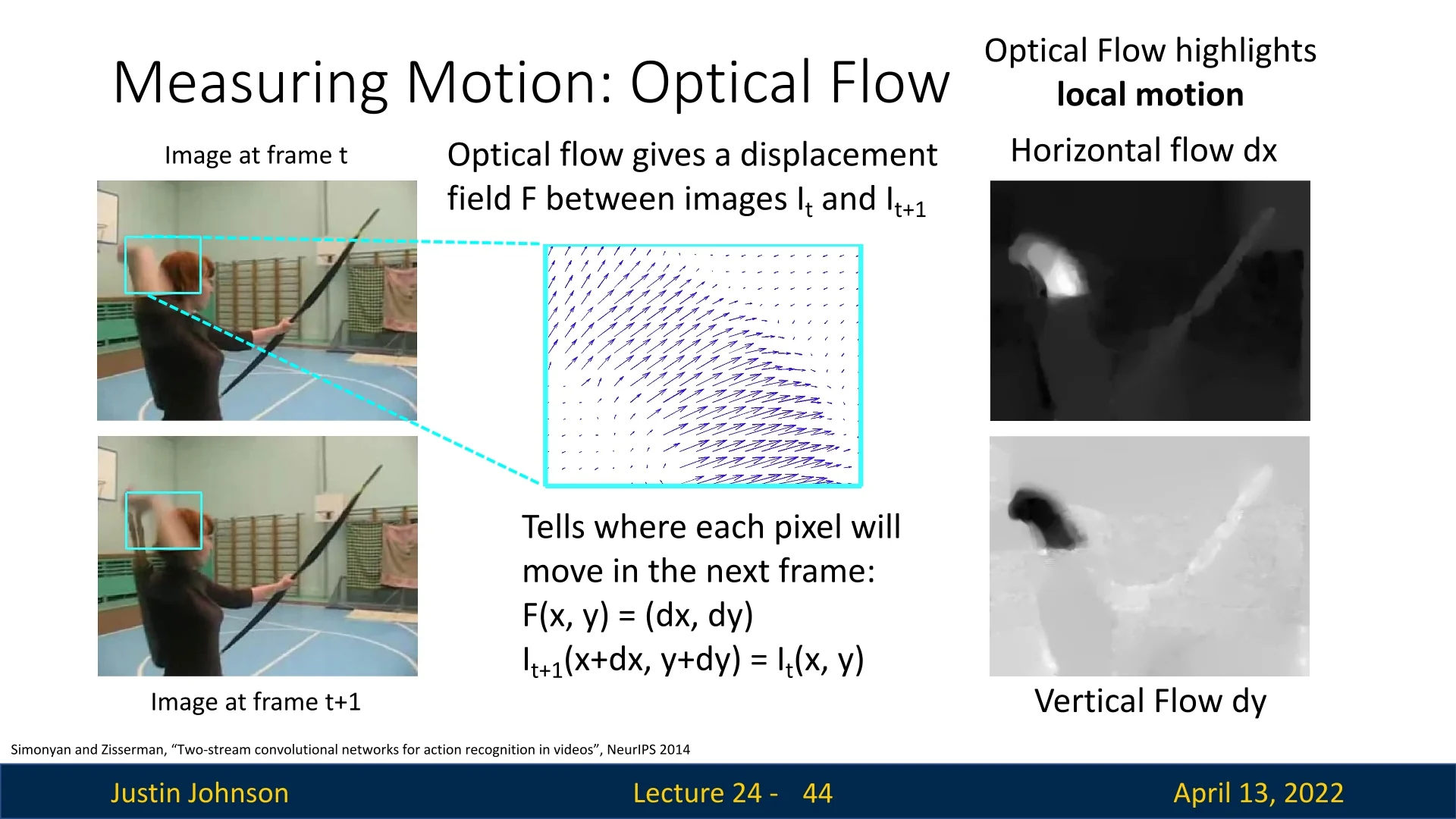
A widely used way to represent motion in videos is through optical flow. At a high level, optical flow estimates how points in one frame move to their new positions in the next frame. \[ F(x,y) = (d_x, d_y), \quad I_{t+1}(x+d_x, y+d_y) \approx I_t(x,y), \] The output is a vector field where \((d_x,d_y)\) is the estimated displacement of the pixel at \((x,y)\) from time \(t\) to \(t+1\). Intuitively, this captures local motion: if an object moves to the right, nearby vectors in the flow field will all point rightward with magnitude proportional to the speed.
Dense vs. sparse flow Optical flow can be dense, with a displacement vector for every pixel, or sparse, with vectors only at keypoints. Dense flow captures detailed motion everywhere, while sparse flow is cheaper and focuses on stable regions.
Why this helps Unlike raw RGB values, which encode only appearance, optical flow provides an explicit description of how things move. This allows models to disentangle appearance (what is present) from motion (how it changes). For example, in an action like “shooting a bow,” the background may be irrelevant, but the flow highlights the arm and bow movement. Feeding these motion fields into CNNs complements RGB inputs and improves video understanding.
24.3.2 Two-Stream Networks
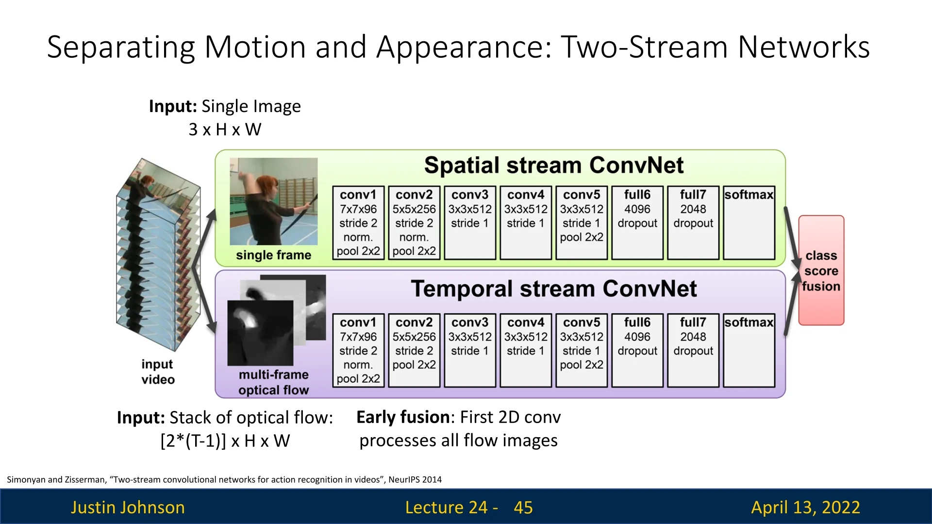
A seminal architecture exploiting this idea is the two-stream network of Simonyan and Zisserman [591]. It consists of two parallel CNN branches:
- Spatial stream: Processes single RGB frames to capture appearance. Each frame is classified independently, and predictions are averaged over \(T\) frames.
- Temporal stream: Processes stacked optical flow fields. From \(T\) frames, there are \(T-1\) optical flows, each with two channels (horizontal and vertical), yielding a tensor of shape \([2(T-1)] \times H \times W\). Early fusion at the first convolution combines motion across frames, followed by standard 2D CNN layers.
At test time, both streams output class distributions. The final prediction is obtained by averaging, or by training an SVM over the concatenated outputs.
Evaluation on UCF-101
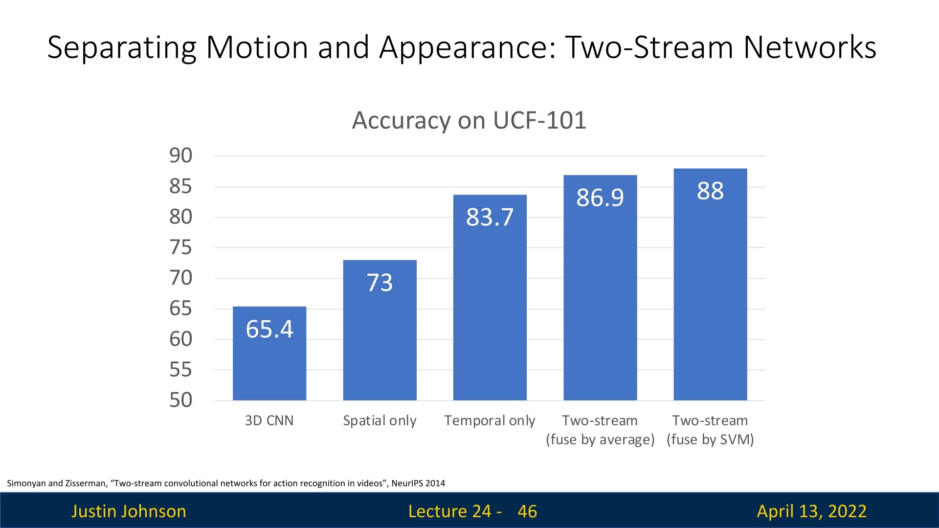
The two-stream model was evaluated on the UCF-101 dataset. Results show clear advantages of separating appearance and motion:
- 3D CNN: \(65.4\%\)
- Spatial-only stream: \(73.0\%\)
- Temporal-only stream: \(83.7\%\)
- Two-stream, average fusion: \(86.9\%\)
- Two-stream, SVM fusion: \(88.0\%\)
These results highlight that motion is often more informative than raw appearance, but the best performance arises when both are combined.
24.4 Modeling Long-Term Temporal Structure
Most architectures discussed so far capture only local temporal patterns: 2D or 3D CNNs operate on short clips of \(\sim \)16–32 frames. Many tasks, however, require reasoning about long-term dependencies, where informative events are separated by seconds or minutes. We therefore seek models that aggregate information across extended time spans while preserving strong spatial representations.
24.4.1 CNN Features + Recurrent Networks
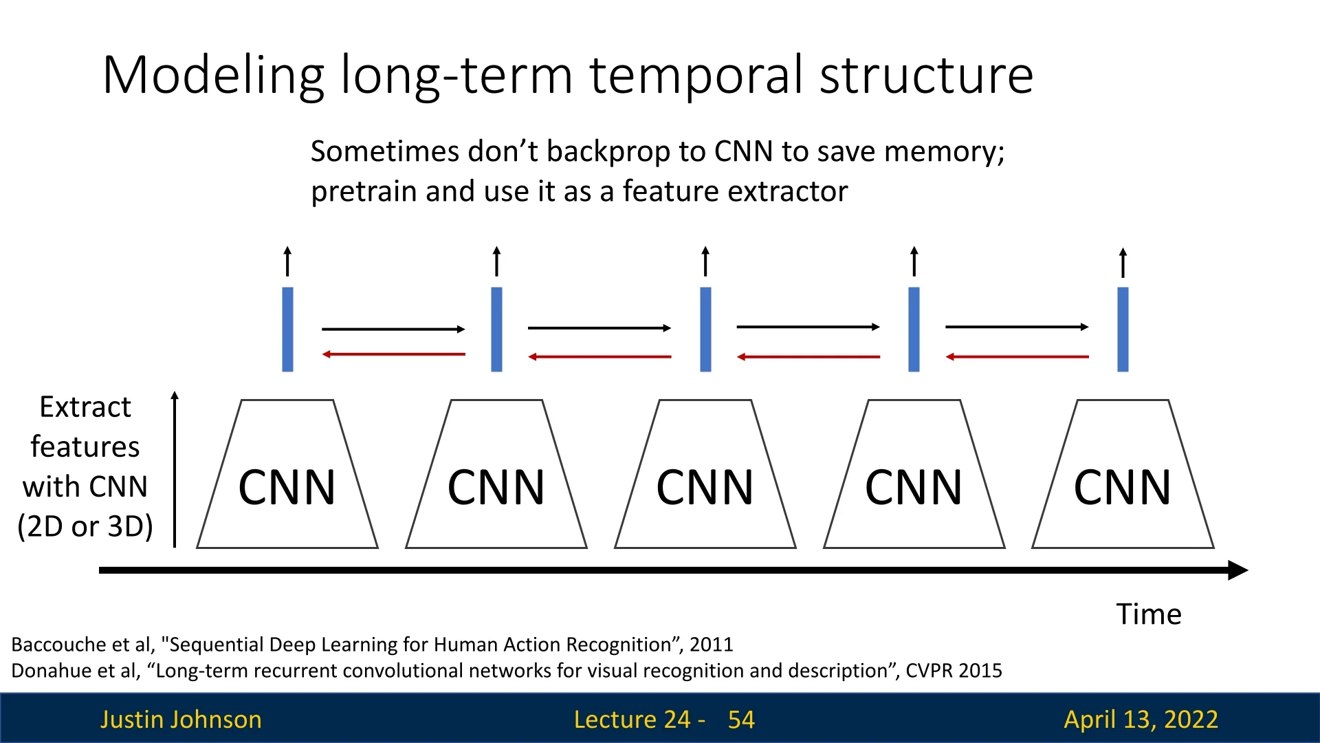
A practical recipe is to pair CNNs for spatial and short-term modeling with RNNs:
- 1.
- Extract per-timestep features with a CNN (2D on frames or 3D on short clips), yielding a feature vector at each step.
- 2.
- Feed the feature sequence to a recurrent model (e.g., LSTM) to aggregate over time.
- 3.
- For video-level classification, use a many-to-one mapping from the final hidden state; for dense labeling, use many-to-many by reading out from all hidden states.
This idea appeared early in Baccouche et al. [21] and was popularized by Donahue et al. with Long-term Recurrent Convolutional Networks (LRCN) [133]. A memory-efficient variant freezes the clip-level CNN (e.g., C3D) and trains only the RNN to cover long time horizons without backpropagating through very long video volumes.
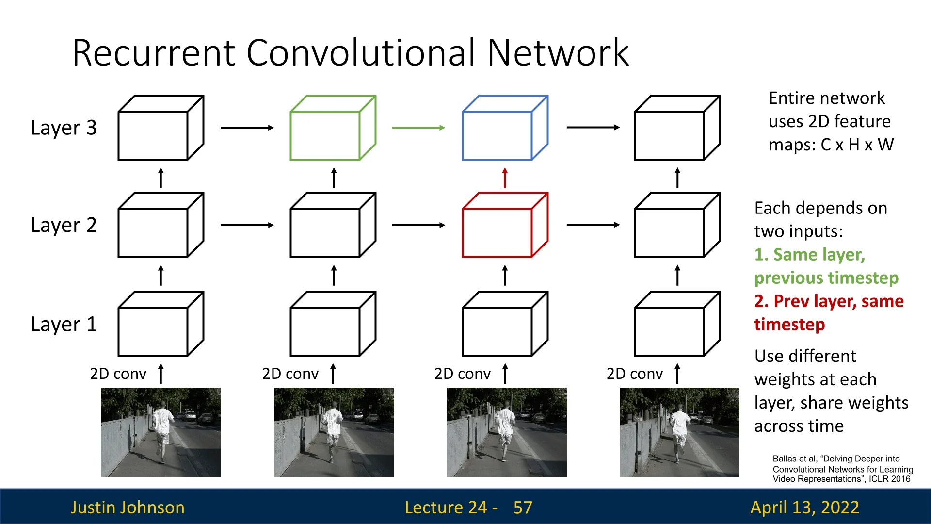
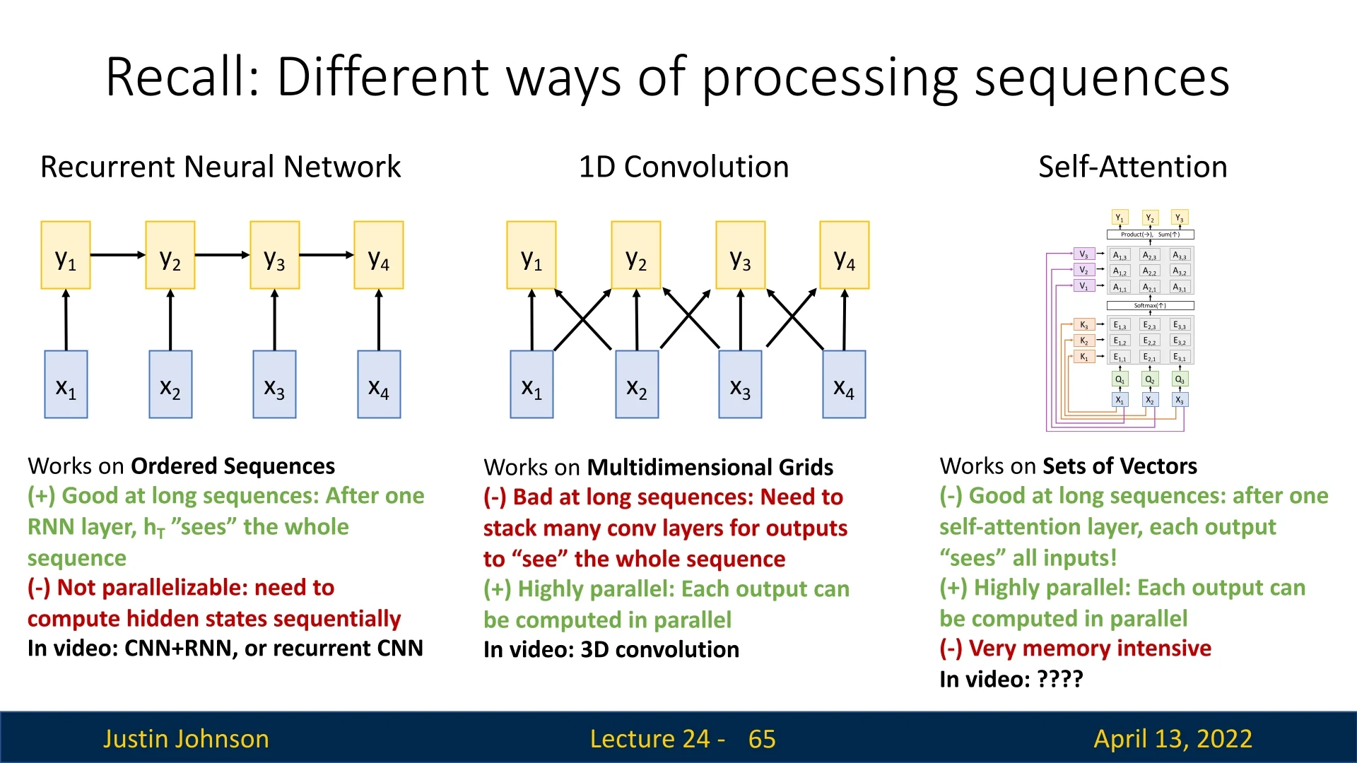
From vector RNNs to recurrent convs Multi-layer RNNs stack temporal processing; the state at time \(t\) in layer \(l\) depends on the state at \((t{-}1,l)\) and on input from \((t,l{-}1)\). The same idea can be applied inside convolutional networks by replacing matrix multiplications with convolutions, yielding recurrent convolutional networks in which each spatial location behaves like a tiny RNN through time [26].
Gated variants and practicality As with standard sequence models, one can replace simple recurrences with GRU or LSTM-style convolutional gates. While elegant, such models inherit the sequential dependency of RNNs, limiting parallelism and slowing training on long videos.
24.4.2 Spatio-Temporal Self-Attention and the Nonlocal Block
Standard 3D CNNs operate on local neighborhoods in space and time; relating distant events requires many layers to propagate information. To address this, Wang et al. [697] proposed the nonlocal block, a spatio-temporal self-attention module that directly connects all positions in a video volume.
Definition Given input features: \begin {equation} \label {eq:chapter24_nonlocal_input} \mathbf {X} \in \mathbb {R}^{C \times T \times H \times W}, \end {equation} the block computes queries, keys, and values via \(1{\times }1{\times }1\) convolutions, \begin {equation} \label {eq:chapter24_nonlocal_qkv} \mathbf {Q},\mathbf {K},\mathbf {V} \in \mathbb {R}^{C' \times T \times H \times W}, \end {equation} flattens space–time so \(N{=}T\!\cdot \!H\!\cdot \!W\), forms affinities \begin {equation} \label {eq:chapter24_nonlocal_attn} \mathbf {A}=\mbox{softmax}\!\big (\mathbf {Q}^\top \mathbf {K}\big )\in \mathbb {R}^{N\times N},\quad \sum _j \mathbf {A}_{ij}=1, \end {equation} aggregates values \begin {equation} \label {eq:chapter24_nonlocal_agg} \mathbf {Y}=\mathbf {V}\,\mathbf {A}^\top \in \mathbb {R}^{C'\times N}, \end {equation} reshapes back to \(C'\times T\times H\times W\), projects to \(C\) channels with \(W_z\), and adds a residual: \begin {equation} \label {eq:chapter24_nonlocal_residual} \mathbf {Z}=W_z(\mathbf {Y})+\mathbf {X}. \end {equation}
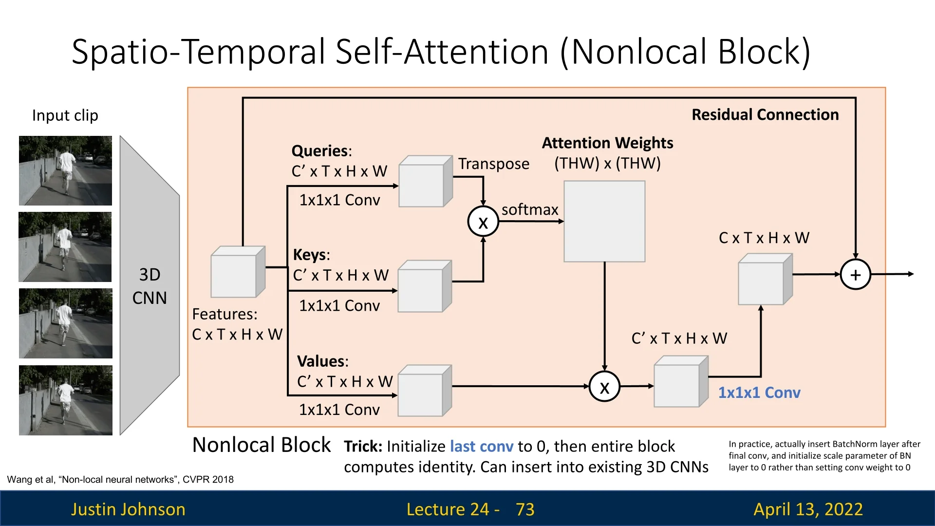
Initialization and integration For stable insertion into 3D CNNs, initialize the final projection so the block starts as identity; in practice, place a BatchNorm after the last \(1{\times }1{\times }1\) and initialize its scale to zero. This yields slow fusion via local 3D convolutions plus global fusion via nonlocal attention.
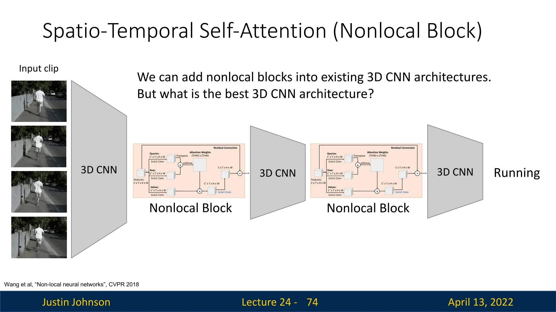
Takeaway Nonlocal blocks overcome locality constraints of convolutions and the sequential bottleneck of RNNs by enabling each position to directly gather context from anywhere in the video, improving representations for tasks such as action recognition and video classification.
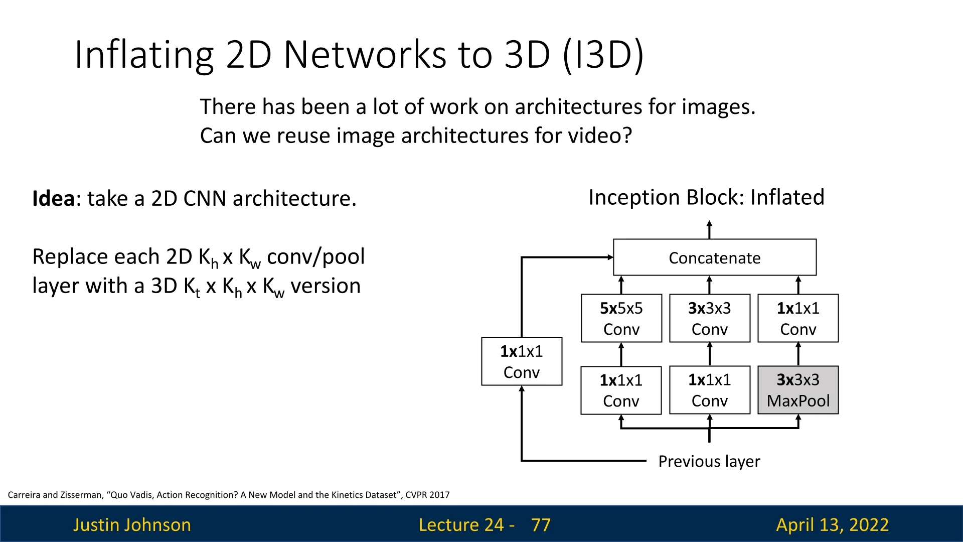
24.4.3 Inflating 2D Networks to 3D (I3D)
Designing effective 3D CNNs from scratch is costly. I3D [74] addresses this by inflating a strong 2D architecture (e.g., Inception-v1) into 3D so it can process space and time while reusing ImageNet-pretrained weights. The core idea is twofold:
- Inflate the architecture: add a temporal extent \(K_t\) to every operation (convolutions, pooling, etc.), turning \(K_h{\times }K_w\) kernels into \(K_t{\times }K_h{\times }K_w\).
- Inflate the weights: initialize 3D kernels from pretrained 2D kernels by replicating them along the temporal dimension and scaling by \(1/K_t\), so the inflated network behaves identically to the 2D parent on static videos.
Inflating the architecture Every 2D layer is given an explicit temporal kernel size \(K_t\):
- \(K_h{\times }K_w\) conv \(\Rightarrow \) \(K_t{\times }K_h{\times }K_w\) conv, same for pooling.
- Inception branches and residual pathways are expanded analogously, preserving topology and receptive-field design.
- Temporal stride and padding are chosen to control temporal downsampling and receptive-field growth, mirroring spatial design.
Inflating the weights: replication and normalization Let a 2D filter be \(W_{2D}\!\in \!\mathbb {R}^{C_\mbox{out}\times C_\mbox{in}\times K_h\times K_w}\) and its inflated 3D filter be \(W_{3D}\!\in \!\mathbb {R}^{C_\mbox{out}\times C_\mbox{in}\times K_t\times K_h\times K_w}\). I3D initializes \begin {equation} \label {eq:chapter24_i3d_weight_inflate} W_{3D}[:,:,t,:,:] \;=\; \tfrac {1}{K_t}\, W_{2D} \quad \mbox{for } t=1,\dots ,K_t. \end {equation} That is, replicate the 2D kernel along time and divide by \(K_t\). The division prevents an unintended \(K_t\)-fold amplification of responses.
Why divide by \(K_t\) Consider a static video \(I\) where every frame is identical. A 3D convolution with the replicated kernel computes a temporal sum of identical 2D responses. Without normalization, \[ \mbox{Conv3D}(W_{3D}, I) \;=\; \sum _{t=1}^{K_t}\mbox{Conv2D}(W_{2D}, I) \;=\; K_t\,\mbox{Conv2D}(W_{2D}, I). \] Scaling by \(1/K_t\) in (24.9) cancels this factor, yielding \[ \mbox{Conv3D}(W_{3D}, I) \;=\; \mbox{Conv2D}(W_{2D}, I), \] so the inflated 3D layer is exactly equivalent to the original 2D layer on static inputs. This preserves activation magnitudes and the semantics of pretrained features at initialization, which is crucial for stability with BatchNorm and deep stacks.
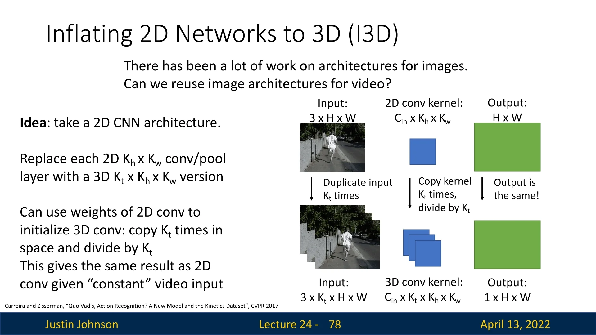
Why inflation is a natural fit Videos contain the same spatial structures as images (edges, textures, objects), now evolving over time. Inflation transfers mature spatial detectors from 2D while introducing a neutral temporal prior (identical slices). During fine-tuning, backpropagation learns temporal asymmetries across slices (e.g., detectors of motion direction or temporal phase), turning static spatial filters into motion-sensitive spatiotemporal filters. Thus, optimization focuses on temporal modeling rather than relearning spatial basics.
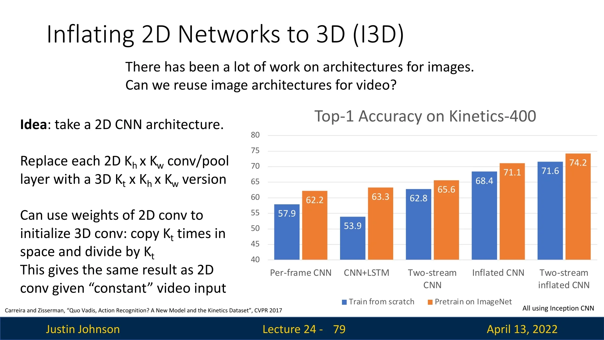
Evidence on Kinetics-400 On Kinetics-400 [294] (300K ten-second YouTube clips across 400 actions), Carreira and Zisserman showed that, with the same Inception-v1 backbone, inflating ImageNet-pretrained weights outperforms training 3D kernels from scratch.
Takeaway I3D provides a principled initialization with several benefits:
- Equivalence on static inputs: the inflated network is provably identical to its 2D parent when frames are constant, ensuring stable initialization.
- Spatial competence transfer: pretrained image filters (e.g., from ImageNet) provide strong recognition of edges, textures, and objects without retraining.
- Focus on temporal dynamics: since spatial features are inherited, optimization capacity can concentrate on learning motion-sensitive filters.
Together, these properties make inflation a strong, data-efficient baseline and a reliable foundation for higher-performing video models.
24.4.4 Transformers for Video Understanding
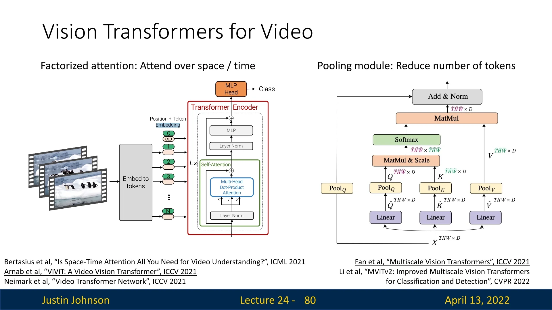
Transformers capture long-range spatio–temporal structure by self-attending over a sequence of tokens. For a clip \(\mathbf {X}\!\in \!\mathbb {R}^{T\times H\times W\times C}\), the video volume is first mapped to \(N\) tokens \(\{z_i\}_{i=1}^N\), then multi-head self-attention (MHSA) relates tokens across space and time [41, 16, 460, 152, 354]. Two core design choices govern effectiveness and efficiency: how to tokenize the video, and how to structure attention so compute and memory remain tractable.
What is a token in video Video tokens are compact spatiotemporal units, not raw pixels:
- Per-frame patches: Split each frame into \(P{\times }P\) patches; the sequence length is \(N=T\cdot \frac {HW}{P^2}\) [16].
- Tubelets (3D patches): Split the video into cuboids of size \(P_t{\times }P{\times }P\), reducing \(N\) by \(\approx P_t\) and embedding short-term motion at input [16, 41].
- CNN feature tokens: Use a 2D CNN per frame and treat spatial feature-map locations as tokens, leveraging ImageNet pretraining and curbing \(N\) [460].
Tokens are linearly projected to \(\mathbb {R}^d\) and enriched with space–time positional information (absolute or relative).
Attention over space and time Full joint attention over all \(N\) tokens costs \(O(N^2)\); with per-frame patches \(N=n_t n_h n_w\) grows multiplicatively in frames \(n_t\) and spatial grid \(n_h\times n_w\) (\(n_h=H/P\), \(n_w=W/P\)). For \(T{=}32\), \(H{=}W{=}224\), \(P{=}16\), we obtain \(N=6272\) and \(\sim 39\)M pairwise interactions per layer per head. To scale, modern designs either factorize attention or pool tokens:
- Divided space–time attention (TimeSformer): Perform spatial attention within each frame, then temporal attention across frames at corresponding spatial sites, reducing cost from \(O((n_t n_h n_w)^2)\) to \(O\!\big (n_t(n_h n_w)^2 + n_h n_w\,n_t^2\big )\) with strong accuracy [41].
- Multiscale transformers (MViT/MViT-v2): Progressively pool tokens in space/time while widening channels, so deeper layers attend over fewer tokens; pooling attention with relative position biases yields excellent accuracy–efficiency trade-offs [152, 354].
- CNN–Transformer hybrids (VTN): Adopt a 2D CNN stem for spatial encoding and use temporal-only transformers on top, exploiting image pretraining and avoiding token explosion [460].
ViViT in depth: tokenization, factorization, computation, and findings ViViT [16] provides a clear blueprint for video transformers, isolating tokenization and attention structure as independent axes.
Tokenization ViViT studies (i) Per-frame patches with uniform frame sampling (\(N=n_t n_h n_w\)) and (ii) Tubelet embedding into \(P_t{\times }P{\times }P\) cuboids (\(N=\lfloor T/P_t\rfloor n_h n_w\)). Tubelets reduce \(N\) linearly in \(P_t\) and inject a motion prior. Initialization matters: inflating 2D patch projections (replicate across \(P_t\) and scale) or central-frame initialization stabilizes training, echoing I3D’s weight inflation.
What “spatial” and “temporal” transformers mean In ViViT’s factorized designs, attention neighborhoods are restricted:
- A Spatial transformer attends within frames to learn objects and layouts; frames can be processed in parallel.
- A Temporal transformer attends across frames at aligned spatial sites (or on frame-level summaries) to learn motion and ordering.
These are standard ViT blocks (MHSA+MLP+residuals); only the token grouping changes.
Architectural variants and compute ViViT compares four designs that trade expressivity for efficiency by constraining who attends to whom. With per-frame patches \(N=n_t n_h n_w\) (\(n_t\) frames, \(n_h{\times }n_w\) patches per frame), joint attention costs \(O(N^2)\); factorized variants decompose this into spatial and temporal parts while preserving the standard Transformer block (MHSA\(\rightarrow \)MLP with residuals and normalization).
- 1.
- Joint spatiotemporal attention: All tokens attend to all others across space and time; maximally expressive but \(O(N^2)\), practical only for short clips or coarse patching.
- 2.
- Factorized encoder: Spatial-only transformers process each frame to produce frame embeddings, then a temporal-only transformer aggregates across frames; \(\approx O\!\big (n_t(n_h n_w)^2\big ) + O\!\big (n_h n_w\,n_t^2\big )\) and spatial stages parallelize over frames.
- 3.
- Factorized self-attention: Within each block, apply spatial attention (within-frame) then temporal attention (across-frame at aligned sites); similar complexity to the factorized encoder with different information flow and regularization.
- 4.
- Factorized dot-product attention: Split attention heads into spatial-only and temporal-only inside a joint block, keeping parameter count while shrinking effective neighborhoods and compute.
With tubelets, \(n_t \leftarrow \lfloor T/P_t \rfloor \), so the temporal term \(O(n_h n_w\,n_t^2)\) becomes \(O\!\big (n_h n_w\,(T/P_t)^2\big )\), explaining why modest \(P_t\) yields substantial savings without sacrificing short-range motion cues.
Positioning relative to contemporaries
- TimeSformer [41]: Also factorizes space–time within blocks; ViViT broadens the design space (encoder- vs. block-level factorization, tubelets, initialization) and clarifies trade-offs.
- MViT/MViT-v2 [152, 354]: Add hierarchical token pooling and pooling attention with relative biases for strong accuracy–efficiency; ViViT serves as a transparent baseline isolating tokenization and factorization without a pyramid.
- VTN [460]: Uses a 2D CNN spatial stem with temporal transformers to curb tokens and leverage image pretraining; ViViT shows pure-transformer backbones can compete when tokenization and factorization are well chosen.
Practical guidance and empirical takeaways from ViViT ViViT’s systematic study suggests clear design choices for building effective and efficient video transformers:
- Prefer tubelets: Use modest temporal extent \(P_t\!\in \![2,4]\) to cut tokens, reduce FLOPs, and inject local motion cues. Tubelets generally outperform per-frame patches at matched compute.
- Adopt factorization for scale: Factorized encoders or block-level space–then–time attention retain most of joint attention’s accuracy while allowing longer clips and higher spatial resolution within a fixed budget.
- Encode space–time position: Apply factorized absolute or relative positional signals.
- Leverage large pretraining: Large-scale image pretraining (e.g., ImageNet-21K/JFT) is essential, since training pure video transformers from scratch on modest video datasets underperforms.
- Fewer multi-view passes needed: Efficient factorization makes it possible to process longer clips in a single forward pass, reducing reliance on expensive multi-view testing.
Why transformers for video Transformers provide a global spatiotemporal receptive field in a single layer via content-based self-attention, allowing direct connections between distant events without the deep local stacking of 3D CNNs or the sequential bottlenecks of RNNs. While naive all-to-all attention over \(N\) video tokens costs \(O(N^2)\), practical video transformers curb both \(N\) and the attention neighborhoods through tokenization into tubelets (reducing sequence length and injecting short-range motion cues), attention factorization (space-then-time or encoder-level separation), and multiscale pooling (progressively merging tokens while widening channels), achieving long-range reasoning at tractable compute [41, 16, 152, 354, 460]. The result is a backbone that preserves temporal reasoning capacity while scaling to longer clips and higher resolutions within realistic budgets.
24.4.5 Visualizing and Localizing Actions
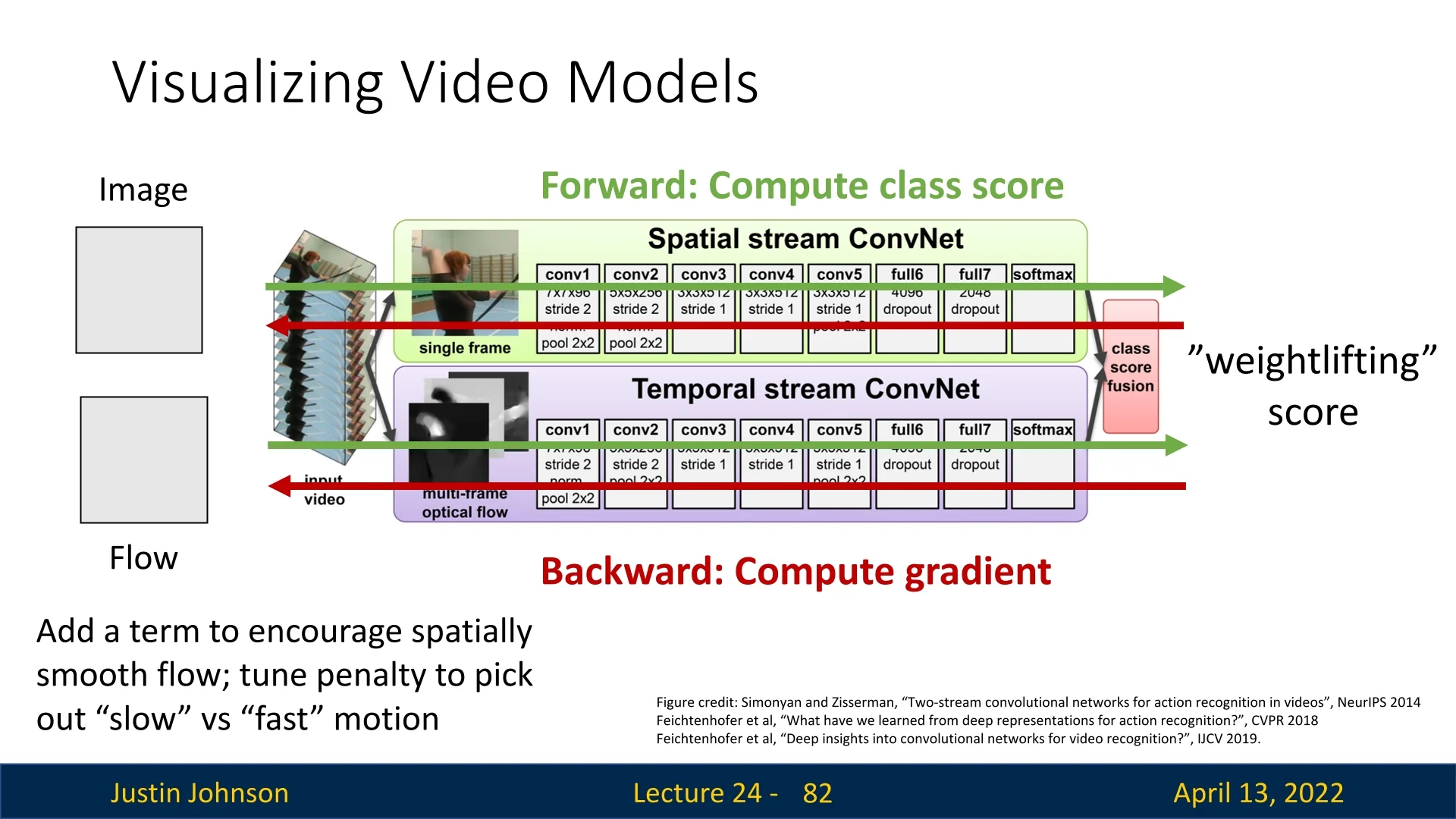
Visualizing Video Models
A useful way to probe what a trained video classifier has learned is to optimize a synthetic video \(\mathbf {V}\!\in \!\mathbb {R}^{C\times T\times H\times W}\) to maximize a class score \(S_c(\mathbf {V})\) while adding priors that favor naturalistic solutions [156, 158]. A generic objective is \begin {equation} \label {eq:chapter24_vis_objective} \max _{\mathbf {V}} \; S_c(\mathbf {V}) \;-\; \lambda _s \,\mathcal {R}_{\mbox{space}}(\mathbf {V}) \;-\; \lambda _t \,\mathcal {R}_{\mbox{time}}(\mathbf {V}), \end {equation} where \(\mathcal {R}_{\mbox{space}}\) encourages spatial smoothness (e.g., spatial total variation) and \(\mathcal {R}_{\mbox{time}}\) encourages temporal coherence (e.g., penalties on finite differences across adjacent frames). By tuning the temporal penalty \(\lambda _t\), one can bias the optimized video toward slow motion (large \(\lambda _t\) suppresses rapid frame-to-frame changes) or fast motion (small \(\lambda _t\) allows rapid changes). This separates appearance cues (what) from motion regimes (how fast), revealing complementary evidence the model uses.
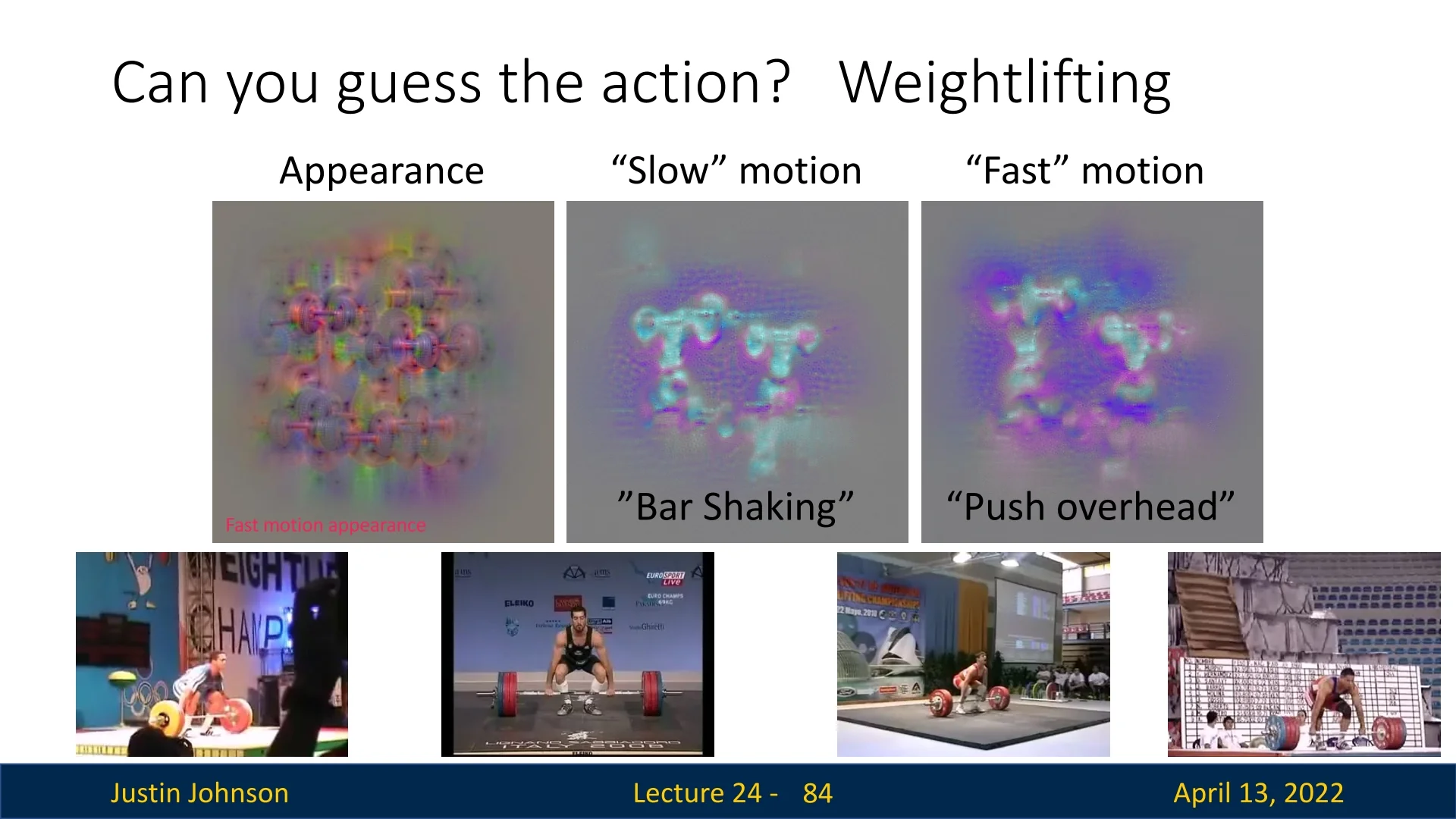
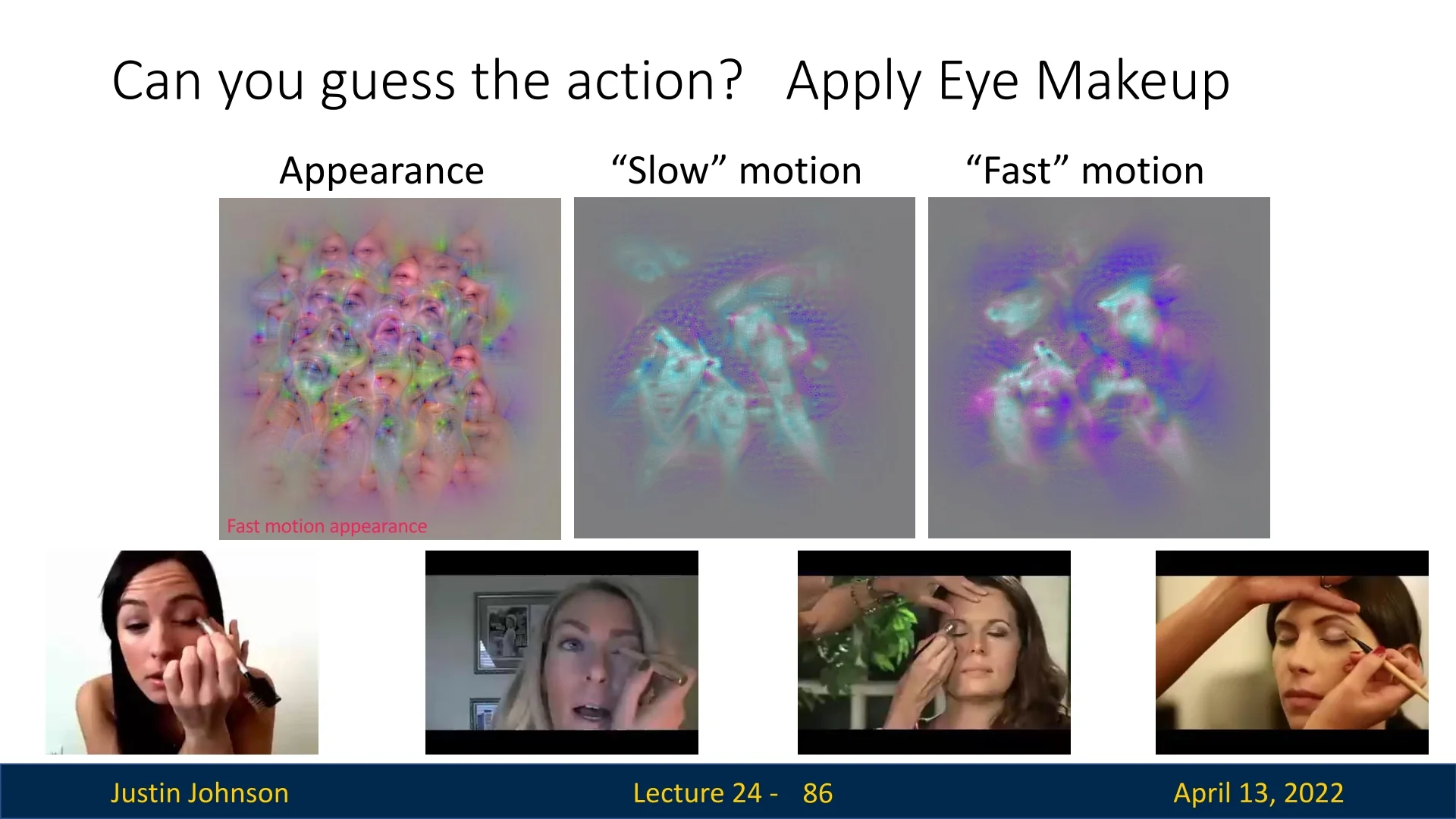
Qualitative examples Optimizing (24.10) for specific classes yields intuitive decompositions into appearance, slow motion, and fast motion channels:
- Weightlifting: The appearance channel emphasizes the barbell and lifter; the slow component accentuates bar shaking; the fast component emphasizes the push overhead—together aligning with the weightlifting concept.
- Apply eye makeup: The appearance channel contains many faces (consistent with makeup tutorials); the slow component captures deliberate hand movements; the fast component highlights brushing strokes.
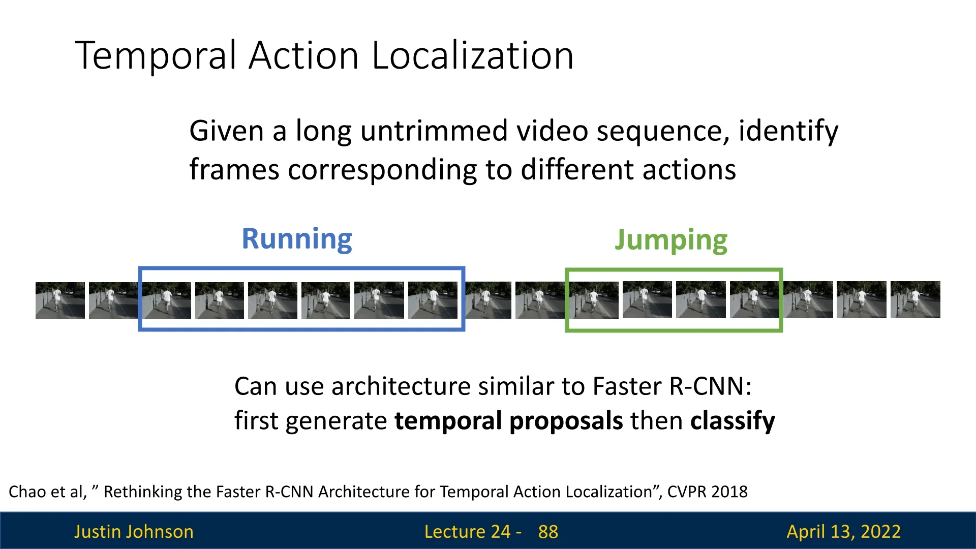
Temporal Action Localization
Problem: Given an untrimmed video, identify the temporal extents of actions and their labels. A popular approach mirrors object detection: first generate temporal proposals, then classify and refine them [78]. Modern systems use 1D temporal anchors or boundary-matching modules coupled with clip-level features from 2D/3D backbones.
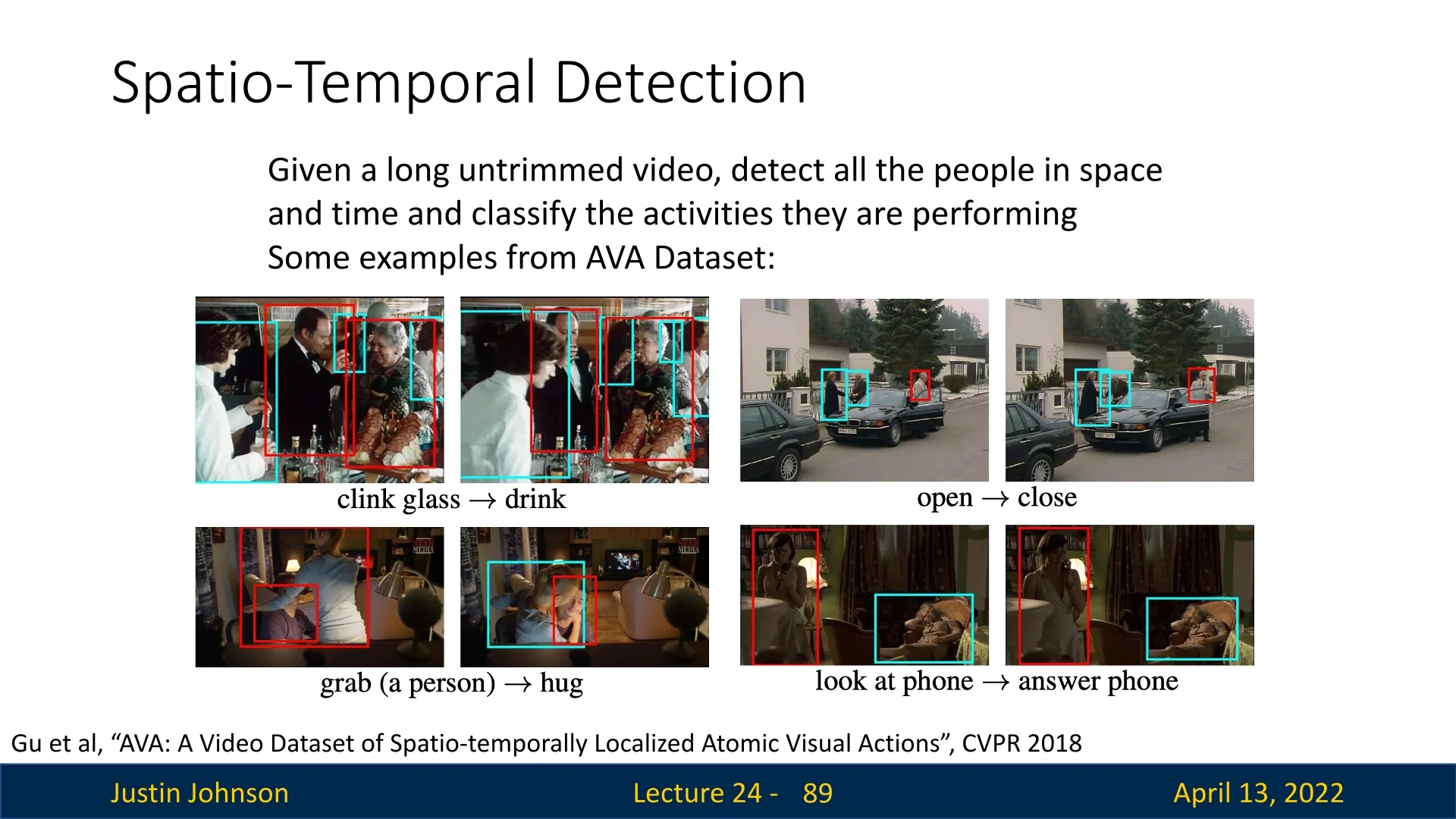
Spatio-Temporal Action Detection
Problem: Detect who does what in space and time: localize people with bounding boxes across frames (tubes) and assign action labels. The AVA dataset provides dense, frame-level annotations of atomic visual actions for people in 15-minute movie clips, enabling research on fine-grained spatiotemporal detection and interaction understanding [197]. Models typically combine per-frame person detection, tube linking, and action classification with temporal context.
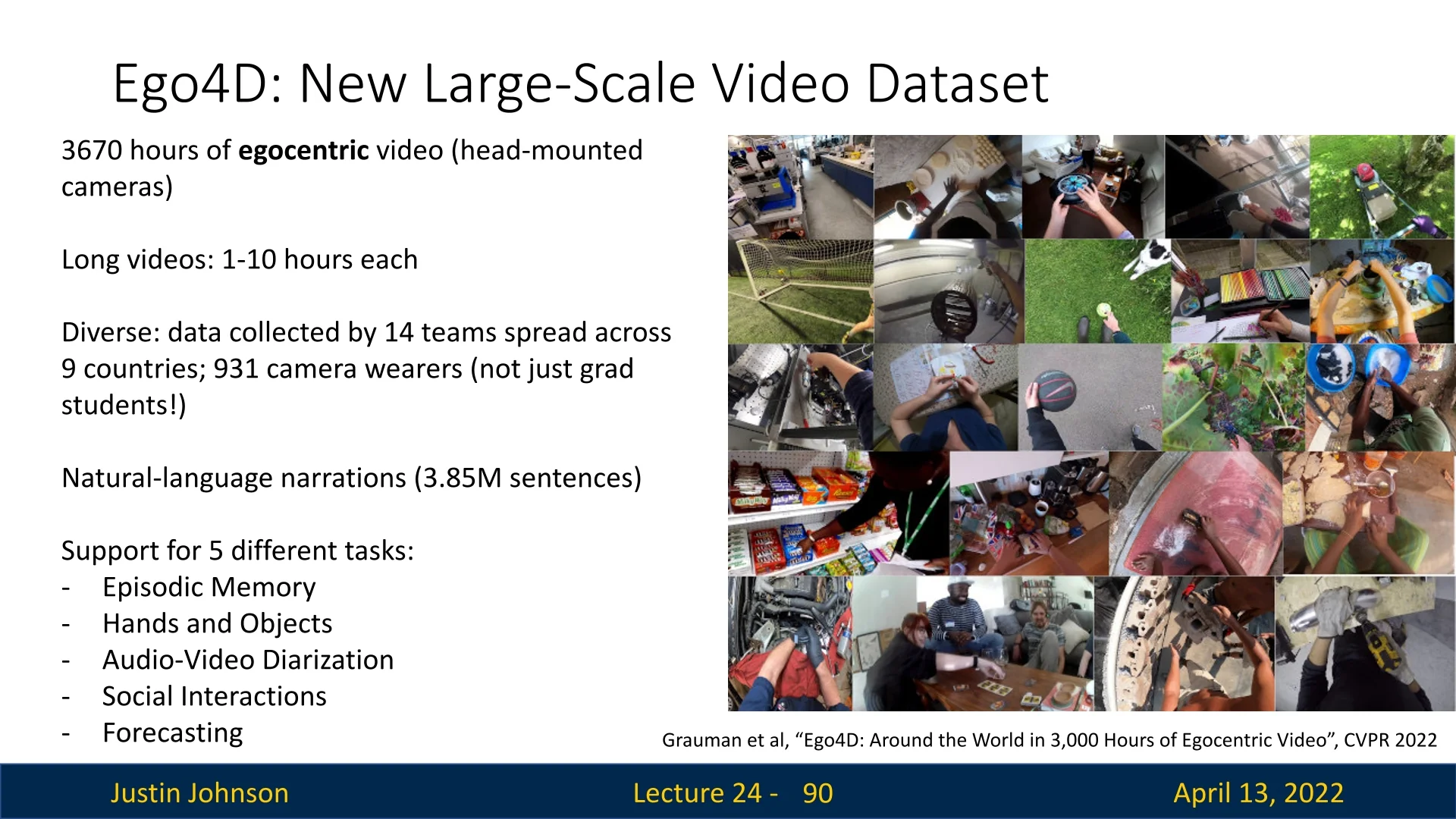
Ego4D: Large-Scale Egocentric Video
Ego4D is a comprehensive egocentric benchmark comprising 3,670 hours of head-mounted, real-world video collected by 14 teams across 9 countries from 931 camera wearers [192]. Videos are long (1–10 hours each) and accompanied by 3.85M natural language narrations. The dataset supports five task families:
- Episodic memory: Retrieve or localize past events based on queries.
- Hands and objects: Detect and track hands and manipulated objects from a first-person perspective.
- Audio–video diarization: Segment and attribute audio–visual events to speakers and sources.
- Social interactions: Recognize and characterize interpersonal behaviors.
- Forecasting: Anticipate future activities or states from ongoing observations.
Enrichment 24.5: Vision–Language Alignment Precursors
The first step toward video–language models was learning how to connect vision and language at scale. As detailed in Section §22, CLIP demonstrated how contrastive alignment could map visual features into a shared language space. Building on this foundation, SigLIP and the BLIP family established the now-standard connector paradigm for mapping visual encoders into LLM-friendly representations. This section focuses on the key image–language precursors that underpin later video systems: SigLIP for improved contrastive alignment, BLIP and BLIP-2 for lightweight vision–LLM bridging, and SigLIP 2 as a stronger, multilingual and dense-capable successor.
Enrichment 24.5.1: SigLIP: Contrastive Alignment with Sigmoid Loss
From CLIP to SigLIP (Intuition First) CLIP learns with a batch–softmax game: in each row/column of the similarity matrix, the true pair must beat all in-batch negatives. This global competition is powerful, but it ties learning quality to batch composition (you need many, diverse negatives), forces expensive all–gathers across devices, and becomes fragile with small or imbalanced batches.
SigLIP [780] changes the game: instead of “one-vs-many” races, it asks a simple yes/no question for each image–text pair—“do they match?”—and trains with a pairwise sigmoid (logistic) loss. By turning alignment into many independent binary decisions, SigLIP:
- Decouples supervision from batch size (every off-diagonal pair is a labeled negative, no global normalization needed),
- Stabilizes gradients (no row/column softmax where a few hard negatives dominate),
- Improves calibration (scores behave like probabilities rather than “who won the batch”),
- Cuts memory & comms (no all–gathers to normalize across the full batch).
Algorithmic Formulation and Intuition With \(n\) image embeddings \(x_i\) and text embeddings \(y_j\) (both L2-normalized), CLIP builds \(S_{ij}{=}x_i^\top y_j\) and optimizes two batch–softmax losses (image\(\!\to \!\)text and text\(\!\to \!\)image): \[ \mathcal {L}_{\mbox{CLIP}} =\frac {1}{2}\!\left [ \frac {1}{n}\sum _{i=1}^{n}\!-\log \frac {\exp (\tau S_{ii})}{\sum _{j=1}^{n}\exp (\tau S_{ij})} + \frac {1}{n}\sum _{j=1}^{n}\!-\log \frac {\exp (\tau S_{jj})}{\sum _{i=1}^{n}\exp (\tau S_{ij})} \right ], \] where the learned temperature \(\tau \) sharpens the softmax; each positive must outrank all \(n{-}1\) negatives in its row/column.
SigLIP replaces this global competition with a per-pair logistic objective: \begin {equation} \label {eq:chapter24_siglip_loss} \mathcal {L}_{\mbox{SigLIP}} = -\frac {1}{n}\sum _{i=1}^{n}\sum _{j=1}^{n} \log \sigma \!\big (z_{ij}\cdot (t\,x_i^\top y_j + b)\big ), \end {equation} with labels \(z_{ij}{=}1\) for matches (\(i{=}j\)) and \(-1\) otherwise (non-match). The formulation introduces two additional learnable scalars:
- Temperature \(t=\exp (t')\). Instead of learning \(t\) directly, the model learns an unconstrained parameter \(t'\), which is exponentiated to ensure \(t>0\). This acts as a similarity sharpness knob: larger \(t\) magnifies dot products, steepening the logistic curve and pushing probabilities closer to \(0\) or \(1\); smaller \(t\) smooths the curve, reducing overconfidence. Exponentiation guarantees stability while allowing flexible scaling during training.
- Bias \(b\). A learnable offset that shifts the decision boundary of the sigmoid. It helps correct for the extreme class imbalance of the loss: each minibatch has only \(n\) positives but \(n^2-n\) negatives. Without \(b\), the logits for negatives can dominate early optimization, leading to vanishing gradients for positives.
Reading the terms in context:
- \(x_i^\top y_j\): cosine-like similarity between L2-normalized embeddings.
- \(t=\exp (t')\): positive temperature that scales similarities, controlling how confidently pairs are classified.
- \(b\): bias that shifts the sigmoid’s threshold, stabilizing optimization when negatives vastly outnumber positives.
- \(z_{ij}\in \{+1,-1\}\): binary label, turning alignment into independent logistic decisions for each pair—no competition across rows/columns as in CLIP.
CLIP vs. SigLIP—why it matters
- Normalization target. CLIP normalizes within each row/column via softmax (needs the whole batch); SigLIP applies a sigmoid per pair (no batchwise denominator).
- Negatives. CLIP’s signal hinges on the number/hardness of in-batch negatives; SigLIP gets explicit negatives from all off-diagonal pairs, even in modest batches.
- Gradient coupling. CLIP couples all pairs in a row/column (hard negatives can dominate); SigLIP yields decoupled per-pair gradients with lower variance.
- Calibration. CLIP scores reflect “winning the batch”; SigLIP’s probabilities are directly interpretable as match likelihoods.
- Distributed cost. CLIP typically needs global all–gathers; SigLIP can be computed in device-local tiles (see the below part on efficient computation).
# Sigmoid contrastive loss pseudocode (SigLIP)
# img_emb : image embeddings [n, d]
# txt_emb : text embeddings [n, d]
# t_prime, b : learnable temperature and bias
# n : batch size
t = exp(t_prime)
zimg = l2_normalize(img_emb)
ztxt = l2_normalize(txt_emb)
logits = dot(zimg, ztxt.T) * t + b
labels = 2 * eye(n) - ones(n) # +1 on diag (matches), -1 off-diag (non-matches)
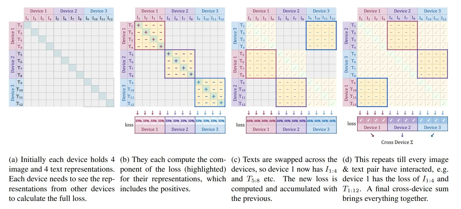
loss = -sum(log_sigmoid(labels * logits)) / nEfficient Implementation The pairwise objective also simplifies distributed training. CLIP’s softmax normalizes over the global batch and thus materializes an \(n{\times }n\) similarity matrix across devices via all-gathers. SigLIP computes the loss locally in chunked blocks, avoiding global normalization and keeping only device-resident tiles in memory. The footprint drops from \(O(n^2)\) to \(O(b^2)\), where \(b\) is the per-device batch size, enabling very large effective batches on comparatively few accelerators. The below figure illustrates the blockwise computation.
Empirical Comparison to CLIP: What Improves in Practice In realistic training settings (small–to–medium batches; noisy web data), SigLIP generally matches or surpasses CLIP while requiring less tuning. The improvements are explained by its pairwise design:
- Batch-size resilience. Because supervision is per pair, SigLIP does not need thousands of negatives per update. Performance scales smoothly up to moderate batch sizes and then plateaus, avoiding CLIP’s reliance on extreme global batches.
- Lower gradient variance. Without a row/column softmax, updates are not dominated by a few hard negatives, yielding smoother optimization and more stable convergence.
- More reliable confidence. Logistic outputs can be interpreted directly as “probability of match”. This leads to better-calibrated similarity scores, making confidence thresholds more trustworthy for retrieval, filtering, or dataset cleaning.
- Robustness to noise. In CLIP, mislabeled or loosely aligned pairs can distort the softmax normalization for a whole row/column. In SigLIP, such outliers only affect their own binary terms, containing the damage and improving robustness on noisy web corpora.
- Efficiency. Losses are computed locally on each device in small blocks, avoiding global all-gathers. This reduces memory and communication costs and makes very large effective batches feasible even on limited hardware.
Impact, Limitations, and Legacy Impact. SigLIP proved that large-scale vision–language alignment can be achieved without global softmax or massive negatives. Its simple, stable recipe made it the backbone for connector-style systems such as BLIP/BLIP-2 (where Q-Former bridges vision encoders to LLMs) and Video-LLMs (where temporal encoders extend SigLIP-style connectors to video).
Limitations. As a purely binary contrastive method, SigLIP:
- Judges only match vs. non-match, lacking multi-way semantics or compositional reasoning.
- Aligns globally but does not yield dense/localized features unless augmented.
- Cannot generate captions or reasoning without an attached LLM.
Legacy. Extensions such as SigLIP 2 [656] add multilingual training, masked prediction, and self-distillation for cross-lingual and localized tasks.
Enrichment 24.5.2: BLIP: Bootstrapping Language–Image Pretraining
High-Level Idea Most large-scale vision–language corpora are scraped from the web by pairing images with their surrounding alt-text—short strings originally written for accessibility or indexing. While attractive for scale, alt-text was never intended as faithful supervision. It is often:
- Missing, e.g. filenames like “IMG_123.jpg” with no descriptive text for the image in its alt text.
- Generic, e.g. “beautiful view” that offers little semantic grounding.
- Off-topic, e.g. boilerplate such as “click here to buy”.
When such noisy associations dominate, models risk learning shortcuts (e.g. linking logos directly to brand names) instead of genuine visual grounding. A second challenge is an objective gap: alt-text resembles retrieval labels more than natural captions or question-answer pairs. Training only with discriminative alignment (as in CLIP) yields strong retrieval but poor generation; training only with captions produces fluent language but weak grounding.
BLIP’s Two-Part Strategy The authors observe that these problems reinforce each other: noisy supervision destabilizes multi-task learning, and narrow objectives fail to transfer broadly. BLIP addresses both with a simple recipe: first curate the data, then train a unified model that can align, ground, and generate.
- Step 1 — Bootstrapping with CapFilt. Instead of trusting raw alt-text, BLIP trains its own Captioner and Filter on a small, clean human-annotated dataset. The Captioner (a generative decoder) produces synthetic captions grounded in visual content, while the Filter (a discriminative encoder) discards both weak alt-text and low-quality synthetic captions. This process rebuilds the large pretraining corpus “from within”, producing cleaner, semantically faithful supervision.
-
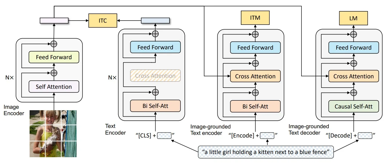
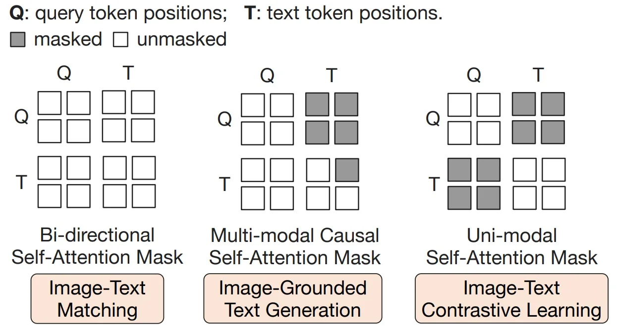
Step 2 — Unified encoder–decoder. BLIP introduces a Multimodal Encoder–Decoder (MED) that supports three complementary modes with largely shared parameters:
- Image–Text Contrastive (ITC). Aligns unimodal encoders for fast retrieval.
- Image–Text Matching (ITM). Uses cross-attention to check whether a caption truly matches an image.
- Language Modeling (LM). Uses a causal decoder to generate captions or answers, reusing the same cross-attention for stable fusion.
By combining these modes, BLIP avoids the trade-off between retrieval strength and generative ability, yielding a single checkpoint that can both discriminate and generate.
Intuition. By first cleaning the data, BLIP removes much of the noise that would otherwise destabilize multi-task optimization. This makes it feasible to train a single model on diverse objectives without one collapsing the others. At the same time, the unified architecture avoids the brittleness of task-specific designs: contrastive alignment alone cannot generate, and pure generation often ignores fine-grained grounding. Combining the two under one framework allows the model to tackle multiple problems at once—retrieval, discrimination, and generation—so that improvements in one skill reinforce the others, producing a more balanced and versatile vision–language learner.
Method
Unified Architecture with Three Functional Modes Rather than building separate networks for retrieval, grounding, and captioning, BLIP uses a single multimodal encoder–decoder backbone that can be run in three different configurations. Most of the heavy components—the vision encoder, cross-attention layers, and feed-forward blocks—are shared across all modes. What changes between them is how attention is applied and which inputs are activated:
- In contrastive alignment, image and text streams run separately without cross-attention.
- In matching, the text stream is augmented with cross-attention over image tokens.
- In generation, the decoder uses causal (masked) self-attention but reuses the same cross-attention and feed-forward layers as the encoder.
This parameter sharing means that improvements in one objective (e.g., better grounding in ITM) flow into the others, stabilizing training and avoiding the need to maintain multiple specialized checkpoints.
- 1.
- Image–Text Contrastive (ITC). The unimodal image encoder and text encoder produce global embeddings. A contrastive loss aligns paired embeddings while pushing apart mismatched ones, giving BLIP strong retrieval and zero-shot transfer.
- 2.
- Image–Text Matching (ITM). The text encoder is extended with cross-attention layers that attend to image features. The model then predicts whether a caption truly matches its paired image. Hard negatives are sampled from ITC to make the discrimination sharper.
- 3.
- Language Modeling (LM). The decoder reuses the same cross-attention and feed-forward blocks as the encoder, but changes the style of self-attention. In the encoder, self-attention is bidirectional: each token can attend to all others, both before and after it, which is ideal for understanding a complete sentence. In contrast, the LM decoder uses causal masking: each token can only attend to those that came earlier in the sequence, never to future tokens. This forces the model to generate text one word at a time, predicting the next token given the history. By combining causal self-attention with cross-attention to the image features, BLIP can produce grounded captions and answers in an autoregressive way, rather than simply classifying pairs.
Why Causal vs. Bidirectional Attention?
- Bidirectional self-attention (ITC, ITM). For understanding tasks, the text stream should read a sentence holistically: each token attends to all others (past and future) to form a context-rich representation. This is ideal for global alignment (ITC) and fine-grained verification (ITM), where the model must judge a complete image–text pair.
- Causal (masked) self-attention (LM). For generation, the decoder must predict the next token given only the prefix; allowing access to future tokens would let it “peek” and trivially copy the target. Causal masking enforces autoregressive decoding and yields fluent, grammatical captions that remain conditioned on the image via cross-attention.
Example. In retrieval or matching, the phrase “a dog on the grass” is compared to an image as a whole—bidirectional attention fits. In captioning, the model writes “A dog is running …” one token at a time—causal masking prevents cheating and maintains coherence.
Objectives in Mathematical Form. BLIP optimizes three complementary losses within the shared backbone:
- Image–Text Contrastive (ITC). For paired embeddings \((v_i, t_i)\) and negatives \((v_i, t_j)\), BLIP applies a symmetric InfoNCE loss: \[ \mathcal {L}_{\mathrm {ITC}} = -\frac {1}{N} \sum _{i=1}^N \Big [ \log \frac {\exp (\mathrm {sim}(v_i,t_i)/\tau )}{\sum _{j=1}^N \exp (\mathrm {sim}(v_i,t_j)/\tau )} + \log \frac {\exp (\mathrm {sim}(t_i,v_i)/\tau )}{\sum _{j=1}^N \exp (\mathrm {sim}(t_i,v_j)/\tau )} \Big ], \] where \(\mathrm {sim}\) is cosine similarity and \(\tau \) a temperature. Intuition: Encourages globally aligned representations so retrieval works out of the box.
- Image–Text Matching (ITM). With image tokens \(v\) and text tokens \(t\), the cross-attentive encoder predicts a binary label \(y \in \{0,1\}\): \[ \mathcal {L}_{\mathrm {ITM}} = - \big [ y \log p(y{=}1|v,t) + (1-y)\log p(y{=}0|v,t) \big ]. \] Intuition: Forces the model to judge whether an entire caption matches an image, sharpening grounding beyond coarse similarity.
- Language Modeling (LM). For a target sequence \(t = (t_1,\ldots ,t_L)\) and image \(v\), the decoder with causal masking maximizes \[ \mathcal {L}_{\mathrm {LM}} = - \sum _{k=1}^L \log p(t_k \mid t_{<k}, v). \] Intuition: Enforces left-to-right text generation conditioned on image features, producing fluent grounded captions.
Together, these objectives form a joint training signal: ITC aligns global spaces, ITM enforces pairwise discrimination, and LM teaches autoregressive generation. Their complementarity stabilizes multi-task learning within one backbone.
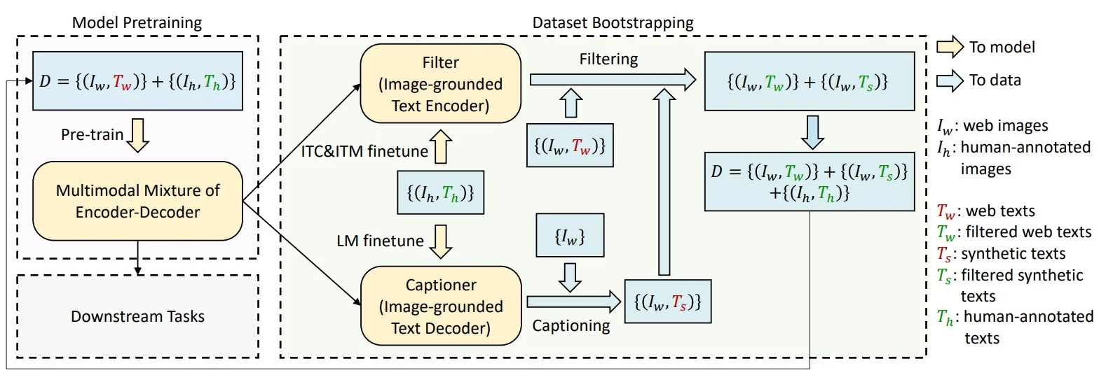
Training Framework: End-to-End Chronology (CapFilt \(\rightarrow \) Final BLIP) Web alt-text is often underspecified or off-topic, which destabilizes pretraining. BLIP therefore separates data construction from final model training in a chronological, three-phase pipeline: (1) train specialized tools, (2) rebuild the dataset, (3) train the final unified model.
- 1.
- Phase 1: Forge the tools on clean data.
- Captioner (generative proposal). Start from a BLIP initialization and fine-tune the image-grounded decoder in LM mode on a small human-annotated set (e.g., COCO). This produces a model that can generate descriptive, image-relevant synthetic captions for web images. Stochastic decoding (e.g., nucleus sampling) increases diversity and coverage.
- Filter (discriminative selection). Independently fine-tune another BLIP initialization in ITM (binary match) with ITC-guided hard negatives on the same clean set. This yields an image–text verifier that can score the semantic fidelity of any pair. Decoupling Captioner and Filter avoids confirmation bias (a generator endorsing its own outputs).
- 2.
- Phase 2: Rebuild the large-scale corpus (CapFilt).
- Generate. Run the Captioner over the web image pool \(\{I_w\}\) to produce synthetic texts \(\{T_s\}\).
- Select. Run the Filter on both sources—the original web texts \(\{T_w\}\) and synthetic texts \(\{T_s\}\)—to keep only high-quality pairs: \[ \{(I_w, T'_w)\} = \mathrm {Filter}\big (\{(I_w, T_w)\}\big ), \qquad \{(I_w, T'_s)\} = \mathrm {Filter}\big (\{(I_w, T_s)\}\big ). \]
- Assemble. Form the bootstrapped pretraining set \[ \mathcal {D}_{\mathrm {boot}} \;=\; \underbrace {\{(I_h, T_h)\}}_{\mbox{human-annotated}} \;\cup \; \underbrace {\{(I_w, T'_w)\}}_{\mbox{filtered web}} \;\cup \; \underbrace {\{(I_w, T'_s)\}}_{\mbox{filtered synthetic}}. \] Here \(T'_w\) and \(T'_s\) denote pairs the Filter judged as matched; images with no good text are dropped.
- 3.
- Phase 3: Train the final unified BLIP on \(\mathcal {D}_{\mathrm {boot}}\).
-
A new BLIP model is initialized and optimized on all three objectives concurrently. In practice, each minibatch is sampled from the same purified dataset \(\mathcal {D}_{\mathrm {boot}}\), and the model routes the inputs through different attention masks and heads depending on the objective:
- ITC (unimodal encoders; no cross-attention) — learns global alignment by comparing embeddings of paired vs. unpaired samples.
- ITM (text encoder with image cross-attention; bidirectional SA) — judges whether a caption matches an image, with hard negatives drawn using ITC similarities.
- LM (decoder with shared cross-attention; causal SA) — generates captions token by token, conditioned on image features.
The total loss is a weighted sum, \[ \mathcal {L} = \lambda _{\mathrm {ITC}} \mathcal {L}_{\mathrm {ITC}} + \lambda _{\mathrm {ITM}} \mathcal {L}_{\mathrm {ITM}} + \lambda _{\mathrm {LM}} \mathcal {L}_{\mathrm {LM}}, \] with all parameters updated jointly.
- Why concurrency matters. Training the three tasks together stabilizes optimization: ITC provides a consistent alignment scaffold, ITM sharpens discrimination using those aligned features, and LM leverages the same cross-attended representations for grounded generation. Running them in parallel avoids forgetting and ensures improvements in one pathway benefit the others.
-
Summary. CapFilt first proposes better text (Captioner) and then selects reliable pairs (Filter). The resulting \(\mathcal {D}_{\mathrm {boot}}\) lets the final BLIP checkpoint learn alignment (ITC), grounding (ITM), and generation (LM) in one backbone—with cross-attention toggled on/off and self-attention switched between bidirectional (understanding) and causal (generation) purely via masks.
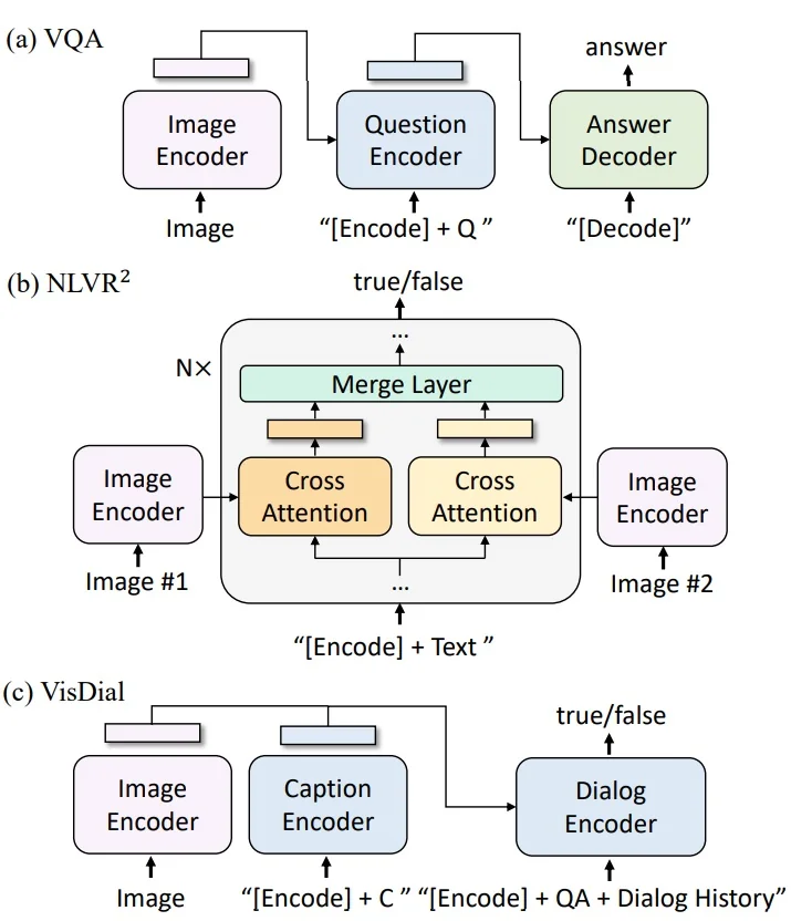
Downstream Usage After pretraining, the same backbone adapts flexibly:
- Retrieval (via ITC and ITM).
- Captioning (via LM).
- VQA (encode question + image, decode answer).
Experiments and Ablations
CapFilt Effectiveness Empirical studies confirm that the CapFilt pipeline provides consistent gains:
- Retrieval and Captioning. Models trained on the cleaned corpus outperform those trained on raw web text, even when both use the same number of image–text pairs.
- Quality vs. Quantity. Adding more noisy pairs does not close the gap; filtering clearly outperforms brute-force scaling, showing that data quality dominates raw scale.
- Retraining vs. Continuing. Restarting training from scratch on the purified set matches or exceeds continuing training on the noisy one, indicating that the benefit comes from improved supervision rather than extra steps.
Ablations Key ablation experiments highlight the necessity of both stages:
- Without Captioner. Relying only on web alt-text leaves a large fraction of pairs irrelevant or underspecified, hurting downstream generation.
- Without Filter. Using synthetic captions without selection reintroduces noise; performance falls sharply, showing that caption generation alone is insufficient.
- Joint vs. Decoupled. Sharing parameters between Captioner and Filter causes confirmation bias and weaker filtering; the decoupled design is essential.
Limitations and Future Work
- Scaling challenges. As models grow, balancing multiple objectives becomes harder; discriminative and generative losses can interfere without careful tuning.
- Dependence on bootstrapping. The final model’s quality is bounded by the effectiveness of the Captioner and Filter; errors in early stages propagate forward.
- Task balance. Equal treatment of ITC, ITM, and LM may not be optimal across domains; different applications may require task-specific weighting.
Toward BLIP-2 BLIP demonstrates that unified multi-task learning is feasible, but scaling to very large LLMs risks overwhelming multimodal fusion. BLIP-2 addresses this by freezing strong pretrained components (a vision encoder and an LLM) and inserting a lightweight connector (the Q-Former) to bridge them, retaining visual grounding while leveraging large-scale language priors.
Enrichment 24.5.3: BLIP-2: Bridging Vision Encoders and LLMs via Q-Former
High-Level Idea BLIP-2 [343] moves away from BLIP’s heavy end-to-end training of both vision and text modules. In BLIP, the ViT image encoder and text transformer were jointly optimized with ITC, ITM, and LM losses. This achieved strong multimodal fusion, but came at huge computational cost: every improvement to the vision or text backbone required retraining the entire model, and the text side remained limited compared to emerging billion-parameter LLMs.
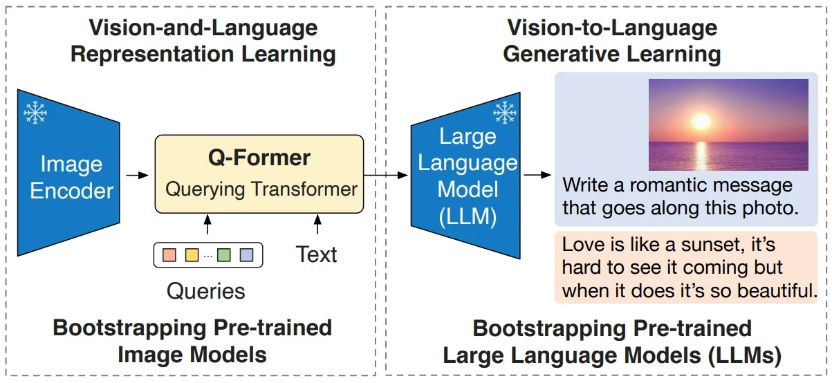
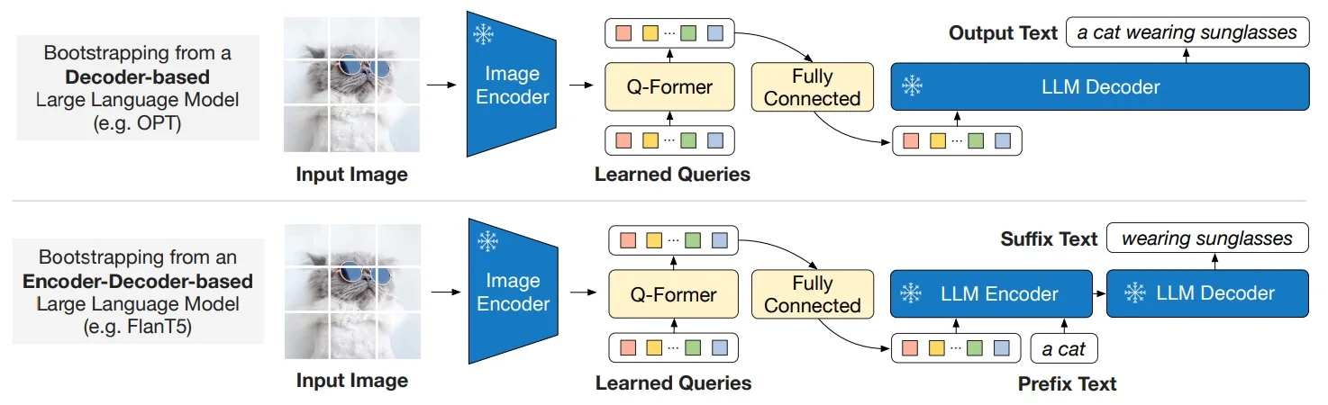
The BLIP-2 shift. Instead of training everything together, BLIP-2 leverages two frozen experts: a large pre-trained ViT (e.g., CLIP ViT-g or EVA-CLIP) and a large pre-trained LLM (e.g., OPT, FlanT5). Both remain untouched, preserving their strong unimodal priors. The only trainable component is a small Querying Transformer (Q-Former), equipped with a fixed set of learnable query tokens. These queries attend to frozen vision features, distill them into a compact representation, and pass them—via a thin projection—as soft prompts into the frozen LLM.
Why a two-stage curriculum? Training the Q-Former to talk to both the vision encoder and the LLM at once is unstable: the LLM has never seen visual tokens and cannot guide the alignment, while the ViT features are too high-dimensional and unstructured for direct prompting. Splitting training stabilizes learning and enforces a clear division of labor: first teach the Q-Former to see with the ViT alone, then teach it to communicate with the frozen LLM.
Two-stage curriculum.
- Stage 1 (Vision–Language Representation Learning): The Q-Former is trained with a frozen ViT, using BLIP-style objectives (contrastive, matching, generation) to ensure its query tokens capture text-relevant visual features. The LLM is not involved.
- Stage 2 (Vision-to-Language Generation): The Q-Former outputs are linearly projected and fed into the frozen LLM. Only the Q-Former is updated, so it learns to “speak the LLM’s language,” turning visual summaries into effective soft prompts for text generation.
In short, BLIP-2 improves over BLIP by freezing powerful unimodal backbones, introducing a small trainable bridge (the Q-Former), and adopting a staged curriculum that first teaches the bridge to see, then teaches it to talk.
Method: A Small Q-Former Bridging Two Frozen Experts
Stage 1: Vision–Language representation with a frozen image encoder Freeze the image encoder (e.g., CLIP/EVA ViT). Train only the Q-Former (and small heads) to extract text-relevant visual summaries. The Q-Former contains \(K\) learnable queries that self-attend and cross-attend to frozen visual tokens. Optimize three objectives (like in 24.4.5.0):
- ITC (Image–Text Contrastive). Learn independent visual/text embeddings for retrieval; align matched pairs and repel mismatches.
- ITM (Image–Text Matching). Enable fine-grained discrimination under bidirectional Q–Text interaction; predict match vs. non-match.
- Image-grounded LM pretraining (masked). Allow text to attend to queries while keeping text causal, preparing queries for generation.
Intuition. ITC yields globally aligned spaces; ITM injects pair-level grounding; masked conditioning prepares Q to act as a compact visual prompt.
Stage 2: Vision-to-language generation with a frozen LLM Keep the LLM frozen. Insert a linear projection from Q-Former outputs to the LLM token space and train (Q-Former + projection) with next-token prediction on caption/instruction data. The LLM consumes the \(K\) projected query tokens prepended to the textual prompt, enabling zero-shot, instruction-following image-to-text generation without tuning the LLM.
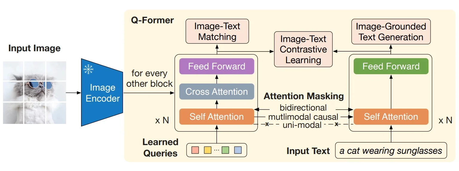
Two-Stage Curriculum: What Trains When and Why Stage 1 (learn to see): Freeze the image encoder; train only the Q-Former on paired image–text data. The three masks in Fig. 24.41 are used jointly so the queries learn to (a) summarize visual content independently of text (ITC), (b) fuse with text for pair verification (ITM), and (c) carry all image information needed to describe the text under causal decoding (image-grounded generation). Intuition: Before “talking” to a frozen LLM, Q must first become a compact, language-relevant summary of the image; otherwise the modality gap is too wide and training is brittle.
Stage 2 (learn to talk): Keep the image encoder and the LLM frozen. Feed the trained queries through a small projection into the LLM’s embedding space and optimize a language-modeling loss while updating only the Q-Former (and the projection). Intuition: With Stage 1, Q already encodes text-relevant visual evidence; Stage 2 teaches Q to present that evidence as a short “soft prompt” the LLM can use without disrupting its linguistic knowledge.
Objectives (concise math + intuition) Let \(v\) denote the Q-aggregated visual embedding and \(t\) a text embedding from the Q-Former stack (mask depends on the objective).
ITC (contrastive, uni-modal mask). \[ \mathcal {L}_{\mbox{ITC}} = -\frac {1}{N}\sum _{i=1}^{N} \Big [ \log \frac {\exp (\langle v_i,t_i\rangle /\tau )}{\sum _{j}\exp (\langle v_i,t_j\rangle /\tau )} + \log \frac {\exp (\langle t_i,v_i\rangle /\tau )}{\sum _{j}\exp (\langle t_i,v_j\rangle /\tau )} \Big ]. \] Why: Learn a shared space where matched pairs are close and mismatches are far, enabling retrieval.
ITM (matching, bi-directional mask). \[ \mathcal {L}_{\mbox{ITM}} = -\frac {1}{N}\sum _{i=1}^{N}\big [y_i\log p_i+(1-y_i)\log (1-p_i)\big ],\quad p_i=\sigma \!\big (W^\top f_{\mbox{fused}}(Q,T)\big ). \] Why: Enforce fine-grained grounding by classifying pair match vs. non-match on fused Q–T features (often with hard negatives).
Image-grounded generation (multimodal causal mask). \[ \mathcal {L}_{\mbox{IG}} = -\sum _{m=1}^{M}\log p\big (y_m \mid y_{<m},\, Q\big ). \] Why: Force queries to carry all image evidence needed for text under causal decoding, making Q a faithful visual prompt.
How the pieces fit during training
- Stage 1 (Q-Former only): Optimize \(\mathcal {L}_{\mbox{ITC}}+\mathcal {L}_{\mbox{ITM}}+\mathcal {L}_{\mbox{IG}}\) with the image encoder frozen and no LLM in the loop. This shapes Q into a compact, language-relevant visual interface.
- Stage 2 (Q-Former + frozen LLM): Project \(Q\) to the LLM’s token space and optimize a standard LM loss \(\mathcal {L}_{\mbox{LM}}=-\sum _m\log p_{\mbox{LLM}}(y_m\mid y_{<m},\,\mathrm {Proj}(Q))\), updating only the Q-Former and projection. This teaches Q to “speak” to the LLM without altering the LLM itself.
| Models | #Trainable Params | Open-sourced? | Visual QA (VQAv2 test-dev) | Image Captioning (NoCaps val) | Image–Text Retrieval (Flickr test)
| |||
|---|---|---|---|---|---|---|---|---|
| VQA acc. | CIDEr | SPICE | TR@1 | IR@1 | ||||
| BLIP [23] | 583M | \(\checkmark \) | – | 113.2 | 14.8 | 96.7 | 86.7 | |
| SimVLM [25] | 1.4B | \(\times \) | – | 112.2 | – | – | – | |
| BEIT-3 [26] | 1.9B | \(\times \) | – | – | – | 94.9 | 81.5 | |
| Flamingo [27] | 10.2B | \(\times \) | 56.3 | – | – | – | – | |
| BLIP-2 | 188M | \(\checkmark \) | 65.0 | 121.6 | 15.8 | 97.6 | 89.7 | |
| Model | #Trainable | Flickr30K Zero-shot (1K) | COCO Finetuned (5K) |
||||||||||
|---|---|---|---|---|---|---|---|---|---|---|---|---|---|
Image\(\rightarrow \)Text | Text\(\rightarrow \)Image | Image\(\rightarrow \)Text | Text\(\rightarrow \)Image |
||||||||||
| R@1 | R@5 | R@10 | R@1 | R@5 | R@10 | R@1 | R@5 | R@10 | R@1 | R@5 | R@10 | ||
Dual-encoder models |
|||||||||||||
| CLIP [28] | 428M | 88.0 | 98.7 | 99.4 | 68.7 | 90.6 | 95.2 | – | – | – | – | – | – |
| ALIGN [29] | 820M | 88.6 | 98.7 | 99.7 | 75.7 | 93.8 | 96.8 | 77.0 | 93.5 | 96.9 | 59.9 | 83.3 | 89.8 |
| FILIP [30] | 417M | 89.8 | 99.2 | 99.8 | 75.0 | 93.4 | 96.3 | 78.9 | 94.4 | 97.4 | 61.2 | 84.3 | 90.6 |
| Florence [31] | 893M | 90.9 | 99.1 | – | 76.7 | 93.6 | – | 81.8 | 95.2 | – | 63.2 | 85.7 | – |
| BEIT-3 [26] | 1.9B | 94.9 | 99.9 | 100.0 | 81.5 | 95.6 | 97.8 | 84.8 | 96.5 | 98.3 | 67.2 | 87.7 | 92.8 |
Fusion-encoder models |
|||||||||||||
| UNITER [32] | 303M | 83.6 | 95.7 | 97.7 | 68.7 | 89.2 | 93.9 | 65.7 | 88.6 | 93.8 | 52.9 | 79.9 | 88.0 |
| OSCAR [33] | 345M | – | – | – | – | – | – | 70.0 | 91.1 | 95.5 | 54.0 | 80.8 | 88.5 |
| VinVL [34] | 345M | – | – | – | – | – | – | 75.4 | 92.9 | 96.2 | 58.8 | 83.5 | 90.3 |
Dual encoder + Fusion encoder re-ranking |
|||||||||||||
| ALBEF [35] | 233M | 94.1 | 99.5 | 99.7 | 82.8 | 96.3 | 98.1 | 77.6 | 94.3 | 97.2 | 60.7 | 84.3 | 90.5 |
| BLIP [23] | 446M | 96.7 | 100.0 | 100.0 | 86.7 | 97.3 | 98.7 | 82.4 | 95.4 | 97.9 | 65.1 | 86.3 | 91.8 |
| BLIP-2 ViT-L | 474M | 96.9 | 100.0 | 100.0 | 88.6 | 97.6 | 98.9 | 83.5 | 96.0 | 98.0 | 66.3 | 86.5 | 91.8 |
| BLIP-2 ViT-g | 1.2B | 97.6 | 100.0 | 100.0 | 89.7 | 98.1 | 98.9 | 85.4 | 97.0 | 98.5 | 68.3 | 87.7 | 92.6 |
Experiments & Ablations (Concise)
- Frozen experts preserve priors. Keeping the vision encoder and LLM frozen avoids catastrophic forgetting while enabling strong zero-shot transfer; most gains come from learning the interface (Q-Former + adapter).
- Masking matters. Ablating the uni-modal mask (ITC) degrades retrieval; ablating bidirectional (ITM) weakens grounding; removing causal conditioning harms generation quality—confirming each mask’s role.
- Number of queries (\(K\)). Too few queries underfit fine details; too many inflate compute with diminishing returns. Moderate \(K\) balances fidelity and LLM cost.
- Adapter simplicity. A single linear projection to the LLM embedding space is sufficient; heavier adapters show minor gains at higher cost.
- Curriculum order. Training Stage 1 (alignment/grounding) before Stage 2 (generation) stabilizes instruction-following performance; skipping Stage 1 reduces zero-shot quality.
Limitations & Future Work
Limitations.
- Bottleneck tightness. A fixed small \(K\) can miss region-level or fine-grained details without auxiliary heads/adapters.
- Static queries. Global queries lack explicit spatial/temporal structure; dense grounding or long video reasoning may require hierarchical or region/time-aware queries.
- Frozen LLM. Great for stability, but limits specialization under large domain shifts; PEFT helps but may be insufficient in niche domains.
Future Work.
- Hierarchical querying. Multi-scale or region/time-conditioned queries for dense tasks and long-horizon video.
- Adaptive \(K\). Dynamic selection based on content difficulty and prompt type to trade off detail vs. cost.
- Richer adapters/PEFT. Structured adapters (e.g., LoRA + gating) for selective LLM specialization while preserving generality.
- Unified multimodality. Extending the Q-Former interface to audio/motion and 3D inputs for broader perception–language reasoning.
Enrichment 24.5.4: SigLIP 2: Multilingual & Dense Vision–Language Encoding
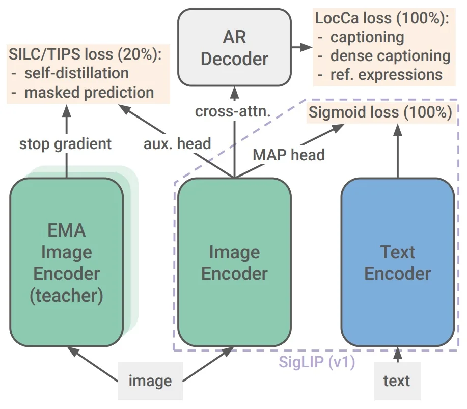
High-Level Overview SigLIP 2 keeps SigLIP’s efficient dual-encoder and pairwise sigmoid loss [780] (no cross-modal attention at test time), and adds training-only signals that teach the vision encoder three missing skills—where evidence is (localization), how patches relate (dense semantics), and how to cope with non-square layouts and non-English text (robustness). Concretely, we add:
- Localization (“where”). A lightweight decoder cross-attends to unpooled patch tokens and is trained for captioning, grounded captioning, and referring expressions [674]. This shapes patch-level spatial semantics but is discarded at test time.
- Dense semantics (“how patches relate”). A late consistency & masking tail (SILC/TIPS) aligns student crops to a full-image EMA teacher and predicts teacher features at masked patches [458, 428], yielding context-aware, part–whole coherent tokens.
- Input robustness (shapes & languages). A brief shape-aware tail either (i) releases size-specific specialists or (ii) trains a single NaFlex generalist that preserves native aspect ratios and supports multiple sequence lengths [117, 43]. Optional active curation improves small models by selecting informative pairs, and a multilingual mix improves cross-lingual transfer.
- Deployment unchanged. All additions are training-only; at inference the model reverts to the original fast SigLIP path: encoder-only dual towers with sigmoid scoring.
Foundational Reminder: How Sigmoid Loss (SigLIP) Works
Before describing the extensions in SigLIP 2, it is useful to recall the idea behind SigLIP [780]. Unlike CLIP, which aligns images and texts by contrasting every pair in a batch through a softmax-normalized InfoNCE loss, SigLIP treats alignment as a set of independent binary classification problems. Each image–text pair is scored by a logistic regressor: true pairs should have high probability, false pairs low. This removes the need for large batches and makes the training objective more flexible, while still encouraging globally aligned embeddings.
Compact formulation (per step) Let \(z^{\mbox{img}}_i, z^{\mbox{text}}_j \in \mathbb {R}^d\) be \(\ell _2\)-normalized embeddings, \(t=\exp (t')\) a learned temperature, and \(b\) a learned bias. The pairwise logit and sigmoid loss are \[ \ell _{ij} \;=\; t \,\big \langle z^{\mbox{img}}_i,\, z^{\mbox{text}}_j \big \rangle + b, \qquad \mathcal {L}_{\sigma } \;=\; - \sum _{i,j}\!\big [y_{ij}\log \sigma (\ell _{ij}) + (1-y_{ij})\log (1-\sigma (\ell _{ij}))\big ], \] with \(y_{ij}=1\) for a true match and \(0\) otherwise. This is the anchor signal that drives SigLIP training.
SigLIP 2 preserves this same core loss, and instead improves the learned representations by layering additional pretraining signals—such as a decoder for localization, late-stage consistency and masking, and resolution/multilingual adaptations—around the dual-encoder backbone. These new ingredients are training-only, leaving inference as efficient as the original SigLIP.
Method: A Staged Curriculum that Teaches Where, Detail, and Robustness
- Main phase (0–80%). Sigmoid image–text alignment plus a lightweight decoder for captioning/grounding: learn global “whether” while injecting “where” so patch tokens carry region evidence early.
- Consistency phase (80–100%). Add self-distillation and masked prediction (no freezing): enforce part–whole agreement and context completion once alignment/captioning are stable.
- Resolution tail (optional). Publish fixed-resolution specialists via short continuations, or train one NaFlex generalist that preserves native aspect ratios across multiple sequence lengths.
- Small-model curation (optional). For ViT-B/16, B/32, apply ACID to select high-learnability pairs and optimize the same sigmoid loss on curated data.
At inference, decoder/teacher/masking/curation are removed; the model is the SigLIP-style dual encoder.
Decoder for captioning and grounding (LocCa-style)
- Role. Add where to SigLIP’s whether: a small Transformer decoder (2–4 layers) cross-attends to unpooled patch tokens during pretraining and is discarded at test time.
-
Mechanism. Optimize three supervised objectives on top of patch tokens: \begin {align*} \mathcal {L}_\text {cap} &= -\sum _{t}\log p(w_t \mid w_{<t}, \{f_p\}) \quad \text {(image captioning)}\\ \mathcal {L}_\text {gcap} &= -\sum _{t}\log p(w_t \mid w_{<t}, \{f_p\}_{p\in \mathcal {R}}) \quad \text {(grounded captioning)}\\ \mathcal {L}_\text {ref} &= -\log \frac {\exp (\langle z_\text {phrase}, z_{\mathcal {R}}\rangle /\tau )}{\sum _k \exp (\langle z_\text {phrase}, z_{\mathcal {R}_k}\rangle /\tau )} \quad \text {(referring expressions)} \end {align*}
where \(f_p\) are patch features, \(\mathcal {R}\) a region (box/mask), and \(z_{\mathcal {R}}\) a pooled region embedding. Region–text pairs are auto-mined with n-grams and open-vocabulary detectors [674]. The combined loss \(\mathcal {L}_\mbox{dec}=\sum \lambda _\bullet \mathcal {L}_\bullet \) is added to the sigmoid anchor.
- Effect. Patch tokens become spatially grounded (who/what/where), improving transfer to grounding/OCR while keeping deployment cost unchanged.
Late self-distillation and masked prediction (SILC/TIPS-style)
- Role. Upgrade patch tokens from global proxies to locally coherent features via two self-supervised signals.
-
Mechanism (added late). Use an EMA teacher (full image) and multiple student views (crops/augments), applied to vision-only augmented views with small weights: \begin {align*} \mathcal {L}_\text {cons} &= \| g(z^\text {pool}_s) - g(z^\text {pool}_t) \|_2^2 \quad \text {(SILC: global consistency)}\\ \mathcal {L}_\text {mask} &= \sum _{m\in \mathcal {M}} \big \| h(f^s_{\setminus m}) - f^t_m \big \|_2^2 \quad \text {(TIPS: masked per-patch completion)} \end {align*}
with one teacher view, eight student crops, EMA decay \(\approx 0.999\), and small projection heads \(g,h\) [458, 428].
- Effect. Crops align with full-image semantics; masked regions are predictable from context. Dense-task transfer improves without any inference change.
Resolution and aspect-ratio adaptation Goal. Eliminate square-warping drift while preserving encoder-only runtime.
- Fixed-resolution continuation (specialists). From \(\sim \)95% progress, resume briefly at a new grid (e.g., \(14{\times }14\!\to \!24{\times }24\)): switch input resize, bilinearly (anti-aliased) retarget 2D positional embeddings \[ PE'_{u',v'}=\sum _{u,v}\alpha _{u,v\to u',v'}\,PE_{u,v},\quad \sum _{u,v}\alpha _{u,v\to u',v'}=1, \] and optionally adapt the patch stem if patch size changes. Continue with the same losses; publish size-specific checkpoints at minimal cost.
- NaFlex variant (one generalist). Train a single checkpoint that preserves native aspect ratios and supports multiple lengths [117, 43]. Per batch: sample \(L\!\in \!\{128,256,576,784,1024\}\); resize so \(H,W\) are patch-size multiples with minimal padding; bilinearly resize the 2D positional grid to \((H,W)\); mask padding in attention/pooling: \[ \mbox{Attn}(Q,K,V,M)=\mbox{softmax}\!\big (\tfrac {QK^\top }{\sqrt {d}}+M\big )V,\quad M_{ij}=\begin {cases}-\infty& \mbox{if pad}\\0&\mbox{otherwise.}\end {cases} \] Omit consistency/masking here for stability. Outcome: one encoder that “bends without warping” on documents/UIs/panoramas with no runtime penalty.
Curation-focused fine-tuning for small models Goal. Lift B-sized checkpoints where data quality, not capacity, is limiting.
- ACID in SigLIP 2 [657]. Distill through data (selection, not logits). For a super-batch \(\mathcal {S}\), score pairs with teacher confidence and student uncertainty, \[ \phi _{ij}=\sigma (\ell ^T_{ij})\cdot H(\sigma (\ell ^S_{ij})),\quad H(p)=-[p\log p+(1-p)\log (1-p)], \] keep the top-\(k\) by \(\phi \), and optimize the same sigmoid loss on this curated subset. A single strong teacher (fine-tuned on a curated billion-pair mix) suffices.
- Effect. Compact models see hard-but-informative pairs, yielding consistent zero-shot/retrieval gains without any inference changes.
Multilingual training mix Goal. Reduce English skew while keeping English strong.
- Design. Include a non-trivial fraction of non-English image–text pairs (e.g., \(\sim \)10%), tokenize with a multilingual tokenizer, and apply simple per-language sampling/balancing; negatives can include cross-language distractors. The objective remains the sigmoid alignment.
- Effect. Better cross-lingual retrieval/classification with negligible English regression; the encoder becomes globally reliable.
Why these additions work (unifying intuition) The decoder teaches where without altering deployment; the SILC/TIPS tail binds parts to wholes and teaches contextual fill-in; shape-aware packing prevents geometric/text distortions; ACID feeds the learner its most informative data; and multilingual mixing broadens alignment beyond English. All are training-only; the shipped model is the same fast SigLIP dual-encoder with weights imprinted for locality, dense semantics, and robustness.
Experiments and Ablations (Concise)
- Across-scales gains (0-shot + retrieval). With comparable compute, SigLIP 2 B/16@256 lifts ImageNet 0-shot from \(76.7\%\) to \(\mathbf {79.1\%}\), COCO T\(\!\to \!\)I R@1 from \(47.4\%\) to \(\mathbf {53.2\%}\), and XM3600 T\(\!\to \!\)I R@1 from \(22.5\%\) to \(\mathbf {40.7\%}\).
- Grounding & referring expressions (decoder teaches “where”). Large REC gains persist after discarding the decoder: B/16@256 RefCOCO val \(64.05\!\to \!\mathbf {83.76}\), testB \(57.89\!\to \!\mathbf {79.57}\); L/16@576 val \(70.76\!\to \!\mathbf {87.28}\), testB \(63.79\!\to \!\mathbf {82.85}\).
- Dense-prediction probes (better patch features). With frozen encoders (So/14@224): PASCAL mIoU \(72.0\!\to \!\mathbf {77.1}\); NYUv2 depth RMSE \(0.576\!\to \!\mathbf {0.493}\); normals improve on both datasets (NYUv2 \(25.9^\circ \!\to \!\mathbf {24.9^\circ }\), NAVI \(26.0^\circ \!\to \!\mathbf {25.4^\circ }\)).
- Late consistency matters (stability without hurting alignment). Add self-distillation + masked prediction only in the last \(\sim \!20\%\) of training (at \(80\%\)), apply on augmented views; weights \(1.0\) (consistency) and \(0.25\) (masked), reweighted by \(\{0.25,0.5,1.0,0.5\}\) for B/L/So400m/g.
- NaFlex helps OCR/docs (native aspect, multi-length). NaFlex outperforms the square model on most OCR/screen retrieval—especially at short sequences; e.g., B/16@256 HierText T\(\!\to \!\)I R@1 \(6.1\!\to \!\mathbf {7.4}\) and Screen2Words I\(\!\to \!\)T \(22.9\!\to \!\mathbf {26.6}\).
- Fixed-resolution specialists (cheap resolution-specific boosts). Short continuations from \(\sim \!95\%\) training produce higher-res checkpoints; for B/16: INet 0-shot \(79.1\!\to \!80.6\!\to \!81.2\) (256/384/512) and COCO T\(\!\to \!\)I R@1 \(53.2\!\to \!54.6\!\to \!55.2\).
- Curated small models (ACID \(\Rightarrow \) stronger B/16, B/32). Brief implicit distillation for B/16,B/32: LR \(10^{-5}\), no WD, \(\sim \)4B extra examples, 0.5 filtering over 64k super-batches—yields the biggest relative gains at B-scale.
- Multilingual mix (global transfer, English intact). Training on WebLI with \(\sim \)90% English / 10% non-English plus de-biasing yields strong cross-lingual retrieval (see XM3600), while keeping English performance high.
- Compute and deployment invariant. The decoder and auxiliary heads are training-only; the released model is the same encoder-only dual tower (swap-in compatible).
What we learn (vs. SigLIP/BLIP/BLIP-2) & which to choose From the results and ablations, SigLIP-2 upgrades the same encoder-only dual tower with stronger what+where features at unchanged runtime: vs. SigLIP it brings robust zero-shot/retrieval gains, large boosts on referring expressions (decoder-imprinted localization), markedly better dense probes (late SILC/TIPS), plus NaFlex and brief high-res continuations for domain/resolution specialization. BLIP targets unified understanding/generation without an external LLM, while BLIP-2 bridges a frozen vision encoder to a frozen LLM via a Q-Former, excelling at open-ended generation but incurring LLM-dependent inference. Which to choose in practice: if you need fast retrieval/classification/grounding with no inference overhead, pick SigLIP-2; if you need text generation (captioning, VQA-style reasoning) without a large LLM, use BLIP; if you need LLM-quality, open-ended outputs or instruction-style prompting, use BLIP-2 (accepting LLM latency/footprint). For an empirical feel of embedding behaviors across baselines (CNN/ViT/CLIP/BLIP-2; note SigLIP-2 is not included), see this concise comparison: Vision](https://pub.towardsai.net/vision-embedding-comparison-for-image-similarity-search-efficientnet-vs-4eac6bf553c4Vision) embedding comparison for image similarity.
Enrichment 24.6: Self-Supervised Video Pretraining for VLLMs
Self-supervised pretraining has become the dominant strategy for learning scalable video backbones, discarding labels in favor of proxy objectives on raw clips (e.g., masked reconstruction or feature prediction). For video-language models, such pretraining is crucial: the LLM can only reason over video content if its encoder supplies rich spatiotemporal representations. This section highlights three representative approaches that defined the state of the art: VideoMAE, which showed the effectiveness of extreme tubelet masking for masked autoencoding [642]; VideoMAEv2, which extended this recipe with dual masking and larger ViTs for improved scalability [685]; and MVD, which replaced pixel targets with teacher features for more semantic supervision [691]. Emerging directions include hybrid masked–contrastive objectives and leveraging complementary signals such as audio or motion priors to further enrich pretraining.
Enrichment 24.6.1: VideoMAE: Masked Autoencoders for Video SSL
Scope and positioning VideoMAE [642] adapts image MAE to videos while explicitly neutralizing temporal shortcuts. Two choices make the objective both difficult and efficient: (i) very high masking that hides 90–95% of tokens from the input clip (a sampled subsequence of \(T\) frames), and (ii) tube masking. In tube masking, a single spatial mask is sampled once on the patch grid and then broadcast across the full temporal span of the clip. Practically, if the spatial patch at \((x,y)\) is selected for masking, that same location is masked in every frame of the clip. A vanilla ViT is used in an asymmetric encoder–decoder: the encoder processes only visible tokens (about 5–10%), and a lightweight decoder reconstructs normalized pixels for the masked tokens. Compared with image MAE, VideoMAE uses higher masking ratios and temporally aligned masks, matching video’s stronger redundancy and preventing frame-to-frame copy shortcuts.
Motivation
Why masked autoencoding for video Videos exhibit slowness and redundancy: adjacent frames are highly similar, so naive per-frame masking leaves near-duplicates visible and enables trivial copying. VideoMAE blocks this shortcut by combining: (i) an extremely high masking ratio (90–95%), and (ii) tube masking that aligns the mask across time. A key point is to separate what the tokens are from how masking is applied:
- Tokens are cubes; masking units are tubes. Tokens are short spatiotemporal cubes (time \(\times \) height \(\times \) width), e.g., \(k{\times }P{\times }P = 2{\times }16{\times }16\). A tube is the stack of all cubes that share a spatial location \((x,y)\) across the entire clip.
- Share one spatial mask across all \(T\) frames. The same 2D mask is repeated over time, so once \((x,y)\) is chosen, all cubes at \((x,y)\) for the clip are hidden. This eliminates frame-to-frame leakage at the same location and forces non-local reasoning.
Step 1 — Tokens are cubes. After temporal subsampling by stride \(\tau \), the \(T\)-frame clip is partitioned into cubes of size \(k{\times }P{\times }P\) (e.g., \(k{=}2\), \(P{=}16\)). Each cube is one token. Let \[ N_t=\frac {T}{k},\qquad N_h=\frac {H}{P},\qquad N_w=\frac {W}{P}, \] so tokens are indexed by \((t',x,y)\) with \(t'\!\in \!\{1,\dots ,N_t\}\) and \((x,y)\!\in \!\{1,\dots ,N_h\}\times \{1,\dots ,N_w\}\).
Step 2 — Masking decisions are made per tube. A tube is the set \(\{(t',x,y): t'=1,\dots ,N_t\}\) at fixed \((x,y)\). Tube masking samples a 2D Bernoulli mask on the spatial grid with ratio \(\rho \): \[ m_{x,y}\sim \mathrm {Bernoulli}(\rho ),\qquad \rho \in \{0.9,0.95\}, \] and broadcasts it along time to define the masked index set \[ \Omega =\{(t',x,y)\mid m_{x,y}=1,\; t'=1,\dots ,N_t\}. \] Thus, although a token (cube) spans only \(k\) frames, the masking unit (tube) spans the full clip length \(T\) (i.e., all \(N_t\) cubes at that \((x,y)\)). If \((x,y)\) is masked, every cube at \((x,y)\) for the clip is masked.
Why this matters. With 90–95% of tubes masked, the encoder receives only \(\approx \)5–10% of tokens and must integrate non-local, long-range space–time cues to reconstruct, instead of copying nearby pixels. The asymmetric design keeps compute low by applying attention only to visible tokens; the lightweight decoder handles reconstruction. Scope note: masking applies only within the sampled \(T\)-frame clip; frames outside the clip are neither seen nor reconstructed in that step.
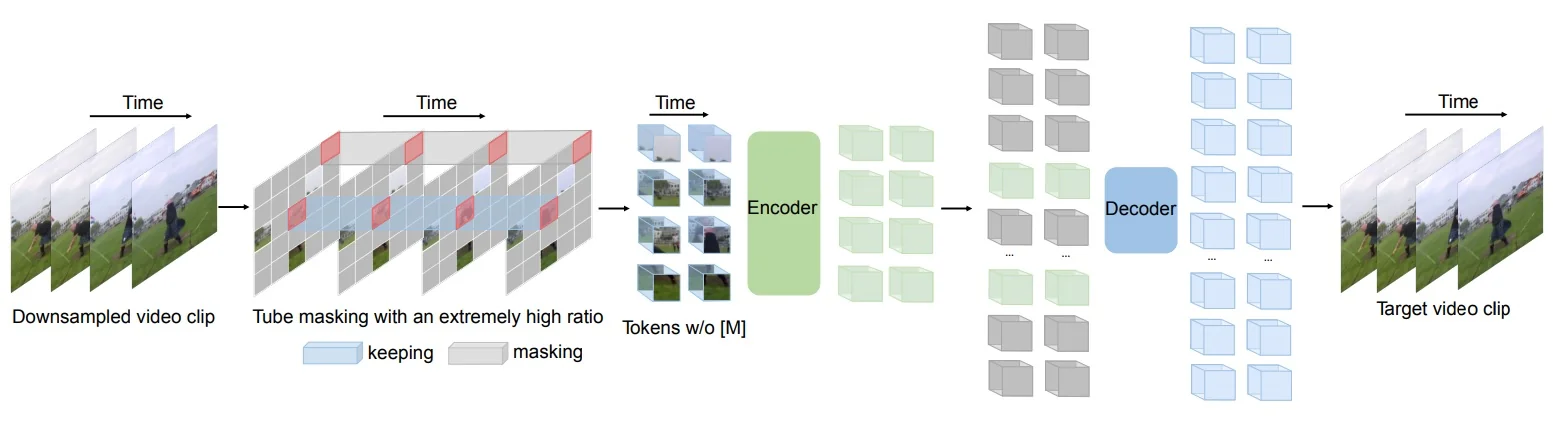
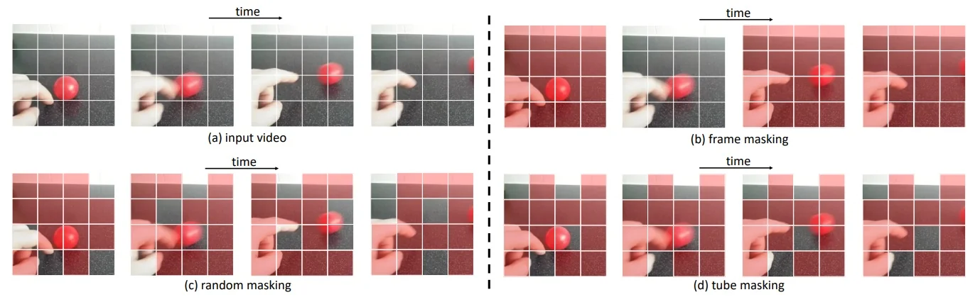
Method
Preliminaries and notation Let a video \(V\) provide a clip of \(t\) consecutive RGB frames. VideoMAE temporally subsamples with stride \(\tau \) to obtain \(T\) frames \(I \in \mathbb {R}^{T \times H \times W \times 3}\). Each frame is partitioned into non-overlapping \(16{\times }16\) patches and packed across time into cubes of size \(2{\times }16{\times }16\); a cube becomes one input token via a linear projection to \(\mathbb {R}^D\). This yields \(\frac {T}{2}\!\times \!\frac {H}{16}\!\times \!\frac {W}{16}\) tokens.
Tube masking with extremely high ratios Let \(\Omega \) denote the set of masked cube indices and \(\rho \in [0,1)\) the masking ratio. Tube masking is applied by sampling a spatial Bernoulli mask once and sharing it across all \(t\): \begin {equation} \label {eq:chapter24_videomae_tube} \mathbb {I}[p_{x,y,\cdot } \in \Omega ] \sim \mathrm {Bernoulli}(\rho )\quad \mbox{with the same outcome for all times}\;, \end {equation} so that if location \((x,y)\) is masked at one frame, it is masked for all frames [642]. Empirically, \(\rho \in \{0.9,0.95\}\) optimizes difficulty and efficiency; lower ratios leave too much redundant evidence, and higher ratios ( \(\geq 0.98\) ) degrade accuracy on SSV2 and K400 (see Fig. 24.47).
Asymmetric encoder–decoder Only visible tokens \(\{z_v\}\) (roughly \((1{-}\rho )\) of all tokens) enter the ViT encoder \(\Phi _{\mbox{enc}}\) with joint space–time attention. A lightweight decoder \(\Phi _{\mbox{dec}}\) receives (i) encoded visible features and (ii) learnable mask tokens as placeholders for \(\Omega \), and predicts reconstructed pixels \(\hat {I}\) for all masked cubes. The asymmetry reduces pre-train cost because expensive self-attention is computed on \(\approx 5{\sim }10\%\) of tokens [642].
Reconstruction objective on masked cubes Following ImageMAE, VideoMAE normalizes pixels per channel and minimizes MSE only over masked positions: \begin {equation} \label {eq:chapter24_videomae_loss} \mathcal {L}_{\mathrm {MAE}} \;=\; \frac {1}{|\Omega |}\sum _{p \in \Omega } \left \| I(p) - \hat {I}(p) \right \|_2^2, \end {equation} where \(p\) indexes masked cubes, \(I\) is the downsampled target clip, and \(\hat {I}\) is the decoder output [642].
- Temporal downsampling. Using stride \(\tau \!\in \!\{4,2\}\) on K400/SSV2 reduces redundancy and balances static and motion cues without collapsing the temporal field of view.
- Cube embedding. 3D tokens (\(2{\times }16{\times }16\)) jointly reduce spatial and temporal lengths, improving efficiency and encouraging space–time reasoning in attention layers.
- Tube masking. Sharing the spatial mask across time removes trivial spatiotemporal correspondences that would otherwise let the model copy from adjacent frames, thereby elevating the task’s semantic level.
- High masking ratio. Videos contain lower information density than images; aggressively masking encourages holistic structure modeling while cutting encoder FLOPs proportionally to \((1{-}\rho )\).
- Pixel-space target and MSE. Reconstructing normalized pixels with MSE outperforms L1 and Smooth-L1 for this setting; predicting only the center frame is inferior to reconstructing the full \(T{\times }\tau \) target.
Algorithmic flow (pseudo code)
# VideoMAE pre-training loop (schematic)
# I: sampled clip of shape [T, H, W, 3]; tau: temporal stride; rho: masking ratio
# enc, dec: ViT encoder/decoder; proj: cube embed; mtoken: learnable mask token

def step(I):
    # 1) Temporal downsampling
    I_tau = I[::tau]  # shape [T, H, W, 3]

    # 2) Cube embedding (2 x 16 x 16) -> tokens
    X = proj(cubeify(I_tau))  # [N_tokens, D]

    # 3) Tube masking: sample a 2D mask once and share across time
    spatial_mask = bernoulli_mask_2d(height=H//16, width=W//16, p=rho)
    tube_mask = repeat_across_time(spatial_mask, repeats=T//2)  # indices omega

    visible, indices_vis = X[~tube_mask], where(~tube_mask)
    masked_indices = where(tube_mask)

    # 4) Encode only visible tokens (asymmetric design)
    H_vis = enc(visible)

    # 5) Prepare decoder sequence: interleave encoded visibles with mask tokens
    Z = stitch_sequence(H_vis, indices_vis, mtoken, masked_indices)

    # 6) Decode to pixel targets for masked cubes and compute loss
    I_hat = dec(Z)                     # predict all cubes; train via masked MSE
    loss = mse(I_hat[masked_indices], I_tau[masked_indices])
    return loss
Architecture, Training, and Datasets
Backbone and attention VideoMAE employs a vanilla ViT with joint space–time self-attention as encoder, so any token can attend to any other across frames and spatial positions. The decoder is shallower and narrower (half channels of encoder; \(4\) blocks by default), which reduces cost while retaining sufficient capacity to reconstruct masked cubes [642].
Training setup The default backbone is ViT-B with \(T{=}16\) frames, cube size \(2{\times }16{\times }16\), and masking ratio \(\rho {=}90\%\). Pre-training runs for \(800\) epochs (on SSV2 and K400) with per-channel pixel normalization and MSE loss on masked cubes. Fine-tuning uses TSN sampling for SSV2 and dense sampling for K400; inference uses \(2{\times }3\) crops on SSV2 and \(5{\times }3\) crops on K400 [642].
Datasets used in experiments and ablations
- K400 (Kinetics-400). \(\sim \)240k YouTube clips over 400 actions; primary large-scale benchmark for pre-training and fine-tuning.
- K700 (Kinetics-700). Extension of Kinetics with 700 classes; used for ablations and AVA detection pre-train variants.
- SSV2 (Something-Something V2). \(\sim \)220k crowd-acted object-manipulation videos with fine-grained motion; used heavily in ablations and to test temporal sensitivity.
- UCF101. 9.5k clips across 101 actions; classic small-scale benchmark, used for transfer evaluation after K400 pre-train.
- HMDB51. 3.5k clips across 51 actions; another small-scale benchmark for transfer experiments.
- AVA v2.2. Atomic Visual Actions detection dataset; used to measure transfer to action detection (mAP), with/without supervised pre-train labels.
- IN-1K / IN-21K. ImageNet-1K/21K; appear in ablations for comparing ImageMAE and supervised ImageNet pre-train baselines.
These datasets cover both large-scale classification (K400/K700, SSV2), small-scale transfer (UCF/HMDB), and detection (AVA), ensuring that VideoMAE is tested across scales and task types.
With this setup established, we now turn to the core experiments and ablations, analyzing how masking ratio, decoder design, targets, and pre-training choices shape performance.
Experiments
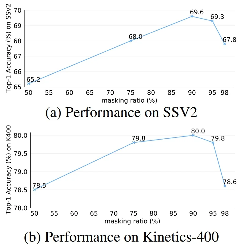
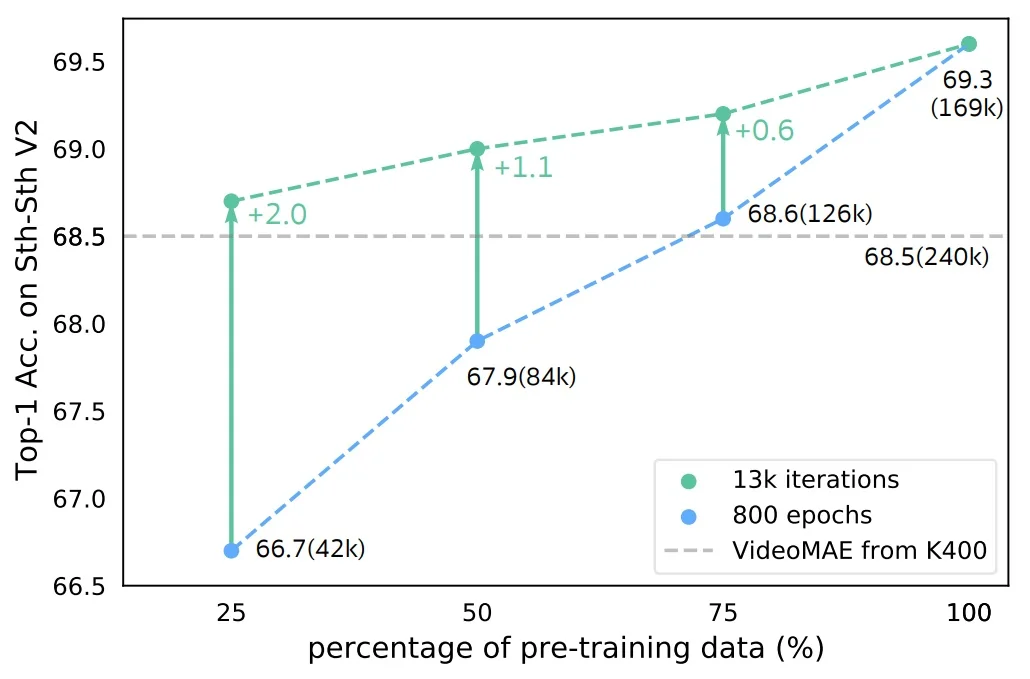
Ablations
| Blocks | SSV2 | K400 | GPU mem. |
| 1 | 68.5 | 79.0 | 7.9G |
| 2 | 69.2 | 79.2 | 10.2G |
| 4 | 69.6 | 80.0 | 14.7G |
| 8 | 69.3 | 79.7 | 23.7G |
What we learn. A shallow, lightweight decoder (4 blocks) is sufficient and most efficient for reconstruction-driven pretraining.
| Case | Ratio | SSV2 | K400 |
| Tube | 75 | 68.0 | 79.8 |
| Tube | 90 | 69.6 | 80.0 |
| Random | 90 | 68.3 | 79.5 |
| Frame\(^\ast \) | 87.5 | 61.5 | 76.5 |
What we learn. Tube masking at very high ratio (90%) is crucial; frame masking creates shortcuts and hurts learning.
| Input | Target | SSV2 | K400 |
| \(T{\times }\tau \) | Center | 63.0 | 79.3 |
| \(T{\times }\tfrac {\tau }{2}\) | \(T{\times }\tfrac {\tau }{2}\) | 68.9 | 79.8 |
| \(T{\times }\tau \) | \(T{\times }\tau \) | 69.6 | 80.0 |
| \(T{\times }\tau \) | \(2T{\times }\tfrac {\tau }{2}\) | 69.2 | 80.1 |
What we learn. Reconstructing the full spatiotemporal target (not just the center frame) yields the best representation.
| Case | SSV2 | K400 |
| From scratch | 32.6 | 68.8 |
| ImageNet-21k sup. | 61.8 | 78.9 |
| IN-21k+K400 sup. | 65.2 | – |
| VideoMAE | 69.6 | 80.0 |
What we learn. Self-supervised VideoMAE pretraining is far stronger than supervised ImageNet initialization for video.
| Dataset | Method | SSV2 | K400 |
| IN-1K | ImageMAE | 64.8 | 78.7 |
| K400 | VideoMAE | 68.5 | 80.0 |
| SSV2 | VideoMAE | 69.6 | 79.6 |
What we learn. In-domain video pretraining (SSV2/K400) is superior to image-only MAE for video recognition.
| Case | SSV2 | K400 |
| L1 loss | 69.1 | 79.7 |
| MSE loss | 69.6 | 80.0 |
| Smooth L1 loss | 68.9 | 79.6 |
What we learn. Masked-pixel MSE is the most effective reconstruction loss in this setting.
| Dataset | Train videos | From scratch | MoCo v3 | VideoMAE |
|---|---|---|---|---|
| K400 | 240k | 68.8 | 74.2 | 80.0 |
| SSV2 | 169k | 32.6 | 54.2 | 69.6 |
| UCF101 | 9.5k | 51.4 | 81.7 | 91.3 |
| HMDB51 | 3.5k | 18.0 | 39.2 | 62.6 |
What we learn. VideoMAE substantially improves over MoCo v3 across diverse datasets, especially on small data (UCF/HMDB).
| Method | Epochs | FT Acc | Lin Acc | Hours | Speedup |
|---|---|---|---|---|---|
| MoCo v3 | 300 | 54.2 | 33.7 | 61.7 | – |
| VideoMAE | 800 | 69.6 | 38.9 | 19.5 | 3.2\(\times \) |
What we learn. Despite more epochs, VideoMAE is far faster in wall-clock and yields much higher accuracy.
| K400\(\rightarrow \)Target | SSV2 | UCF | HMDB |
|---|---|---|---|
| MoCo v3 | 62.4 | 93.2 | 67.9 |
| VideoMAE | 68.5 | 96.1 | 73.3 |
What we learn. VideoMAE features transfer better to both motion-centric (SSV2) and appearance-centric (UCF/HMDB) targets.
| Method | Backbone | Pre-train Dataset | Extra labels | \(T{\times }\tau \) | GFLOPs | Param | mAP |
|---|---|---|---|---|---|---|---|
| supervised [45] | SlowFast - R101 | Kinetics-400 | ✓ | \(8{\times }8\) | 138 | 53 | 23.8 |
| CVRL [46] | SlowOnly - R50 | Kinetics-400 | ✗ | \(32{\times }2\) | 42 | 32 | 16.3 |
| \(\rho \)BYOL\(_{\rho =3}\) [47] | SlowOnly - R50 | Kinetics-400 | ✗ | \(8{\times }8\) | 42 | 32 | 23.4 |
| \(\rho \)MoCo\(_{\rho =3}\) [47] | SlowOnly - R50 | Kinetics-400 | ✗ | \(8{\times }8\) | 42 | 32 | 20.3 |
| MaskFeat\(^{\uparrow 312}\) [48] | MViT - L | Kinetics-400 | ✓ | \(40{\times }3\) | 2828 | 218 | 37.5 |
| MaskFeat\(^{\uparrow 312}\) [48] | MViT - L | Kinetics-600 | ✓ | \(40{\times }3\) | 2828 | 218 | 38.8 |
| VideoMAE [42] | ViT - S | Kinetics-400 | ✗ | \(16{\times }4\) | 57 | 22 | 22.5 |
| VideoMAE [42] | ViT - S | Kinetics-400 | ✓ | \(16{\times }4\) | 57 | 22 | 28.4 |
| VideoMAE [42] | ViT - B | Kinetics-400 | ✗ | \(16{\times }4\) | 180 | 87 | 26.7 |
| VideoMAE [42] | ViT - B | Kinetics-400 | ✓ | \(16{\times }4\) | 180 | 87 | 31.8 |
| VideoMAE [42] | ViT - L | Kinetics-400 | ✗ | \(16{\times }4\) | 597 | 305 | 34.3 |
| VideoMAE [42] | ViT - L | Kinetics-400 | ✓ | \(16{\times }4\) | 597 | 305 | 37.0 |
| VideoMAE [42] | ViT - H | Kinetics-400 | ✗ | \(16{\times }4\) | 1192 | 633 | 36.5 |
| VideoMAE [42] | ViT - H | Kinetics-400 | ✓ | \(16{\times }4\) | 1192 | 633 | 39.5 |
| VideoMAE [42] | ViT - L | Kinetics-700 | ✗ | \(16{\times }4\) | 597 | 305 | 36.1 |
| VideoMAE [42] | ViT - L | Kinetics-700 | ✓ | \(16{\times }4\) | 597 | 305 | 39.3 |
| Method | Backbone | Extra data | Ex. labels | Frames | GFLOPs | Param | Top-1 | Top-5 |
|---|---|---|---|---|---|---|---|---|
| TEINet\(^{\mbox{En}}\) [49] | ResNet50\(\times \)2 | ImageNet-1K | ✓ | \(8{+}16\) | \(99{\times }10{\times }3\) | 50 | 66.5 | N/A |
| TANet\(^{\mbox{En}}\) [50] | ResNet50\(\times \)2 | ImageNet-1K | ✓ | \(8{+}16\) | \(99{\times }2{\times }3\) | 51 | 66.0 | 90.1 |
| TDN\(^{\mbox{En}}\) [51] | ResNet101\(\times \)2 | ImageNet-1K | ✓ | \(8{+}16\) | \(198{\times }1{\times }3\) | 88 | 69.6 | 92.2 |
| SlowFast [45] | ResNet101 | Kinetics-400 | ✓ | \(8{+}32\) | \(106{\times }1{\times }3\) | 53 | 63.1 | 87.6 |
| MViTv1 [14] | MViTv1 - B | Kinetics-400 | ✓ | 64 | \(455{\times }1{\times }3\) | 37 | 67.7 | 90.9 |
| TimeSformer [11] | ViT - B | ImageNet-21K | ✓ | 8 | \(196{\times }1{\times }3\) | 121 | 59.5 | N/A |
| TimeSformer [11] | ViT - L | ImageNet-21K | ✓ | 64 | \(5549{\times }1{\times }3\) | 430 | 62.4 | N/A |
| ViViT FE [12] | ViT - L | IN-21K+K400 | ✓ | 32 | \(995{\times }4{\times }3\) | N/A | 65.9 | 89.9 |
| Motionformer [52] | ViT - B | ImageNet-21K | ✓ | 16 | \(370{\times }1{\times }3\) | 109 | 66.5 | 90.1 |
| Motionformer [52] | ViT - L | ImageNet-21K | ✓ | 32 | \(1185{\times }1{\times }3\) | 382 | 68.1 | 91.2 |
| Video Swin [53] | Swin - B | Kinetics-400 | ✓ | 32 | \(321{\times }1{\times }3\) | 88 | 69.6 | 92.7 |
| VIMPAC [54] | ViT - L | HowTo100M+DALLE | ✗ | 10 | N/A\({\times }10{\times }3\) | 307 | 68.1 | N/A |
| BEVT [55] | Swin - B | IN-1K+K400+DALLE | ✗ | 32 | \(321{\times }1{\times }3\) | 88 | 70.6 | N/A |
| MaskFeat\(^{\uparrow 312}\) [48] | MViT - L | Kinetics-600 | ✓ | 40 | \(2828{\times }1{\times }3\) | 218 | 75.0 | 95.0 |
| VideoMAE [42] | ViT - B | Kinetics-400 | ✗ | 16 | \(180{\times }2{\times }3\) | 87 | 69.7 | 92.3 |
| VideoMAE [42] | ViT - L | Kinetics-400 | ✗ | 16 | \(597{\times }2{\times }3\) | 305 | 74.0 | 94.6 |
| VideoMAE [42] | ViT - S | no external data | ✗ | 16 | \(57{\times }2{\times }3\) | 22 | 66.8 | 90.3 |
| VideoMAE [42] | ViT - B | no external data | ✗ | 16 | \(180{\times }2{\times }3\) | 87 | 70.8 | 92.4 |
| VideoMAE [42] | ViT - L | no external data | ✗ | 16 | \(597{\times }2{\times }3\) | 305 | 74.3 | 94.6 |
| VideoMAE [42] | ViT - L | no external data | ✗ | 32 | \(1436{\times }1{\times }3\) | 305 | 75.4 | 95.2 |
| Method | Backbone | Extra data | Ex. labels | Frames | GFLOPs | Param | Top-1 | Top-5 |
|---|---|---|---|---|---|---|---|---|
| NL I3D [8] | ResNet101 | ImageNet-1K | ✓ | 128 | \(359{\times }10{\times }3\) | 62 | 77.3 | 93.3 |
| TANet [50] | ResNet152 | ImageNet-1K | ✓ | 16 | \(242{\times }4{\times }3\) | 59 | 79.3 | 94.1 |
| TDN\(^{\mbox{En}}\) [51] | ResNet101 | ImageNet-1K | ✓ | \(8{+}16\) | \(198{\times }10{\times }3\) | 88 | 79.4 | 94.4 |
| TimeSformer [11] | ViT - L | ImageNet-21K | ✓ | 96 | \(8353{\times }1{\times }3\) | 430 | 80.7 | 94.7 |
| ViViT FE [12] | ViT - L | ImageNet-21K | ✓ | 128 | \(3980{\times }1{\times }3\) | N/A | 81.7 | 93.8 |
| Motionformer [52] | ViT - L | ImageNet-21K | ✓ | 32 | \(1185{\times }10{\times }3\) | 382 | 80.2 | 94.8 |
| Video Swin [53] | Swin - L | ImageNet-21K | ✓ | 32 | \(604{\times }4{\times }3\) | 197 | 83.1 | 95.9 |
| ViViT FE [12] | ViT - L | JFT-300M | ✓ | 128 | \(3980{\times }1{\times }3\) | N/A | 83.5 | 94.3 |
| ViViT [12] | ViT - H | JFT-300M | ✓ | 32 | \(3981{\times }4{\times }3\) | N/A | 84.9 | 95.8 |
| VIMPAC [54] | ViT - L | HowTo100M+DALLE | ✗ | 10 | N/A\({\times }10{\times }3\) | 307 | 77.4 | N/A |
| BEVT [55] | Swin - B | IN-1K+DALLE | ✗ | 32 | \(282{\times }4{\times }3\) | 88 | 80.6 | N/A |
| MaskFeat\(^{\uparrow 352}\) [48] | MViT - L | Kinetics-600 | ✗ | 40 | \(3790{\times }4{\times }3\) | 218 | 87.0 | 97.4 |
| ip-CSN [56] | ResNet152 | no external data | ✗ | 32 | \(109{\times }10{\times }3\) | 33 | 77.8 | 92.8 |
| SlowFast [45] | R101+NL | no external data | ✗ | \(16{+}64\) | \(234{\times }10{\times }3\) | 60 | 79.8 | 93.9 |
| MViTv1 [14] | MViTv1 - B | no external data | ✗ | 32 | \(170{\times }5{\times }1\) | 37 | 80.2 | 94.4 |
| MaskFeat [48] | MViT - L | no external data | ✗ | 16 | \(377{\times }10{\times }1\) | 218 | 84.3 | 96.3 |
| VideoMAE [42] | ViT - S | no external data | ✗ | 16 | \(57{\times }5{\times }3\) | 22 | 79.0 | 93.8 |
| VideoMAE [42] | ViT - B | no external data | ✗ | 16 | \(180{\times }5{\times }3\) | 87 | 81.5 | 95.1 |
| VideoMAE [42] | ViT - L | no external data | ✗ | 16 | \(597{\times }5{\times }3\) | 305 | 85.2 | 96.8 |
| VideoMAE [42] | ViT - H | no external data | ✗ | 16 | \(1192{\times }5{\times }3\) | 633 | 86.6 | 97.1 |
| VideoMAE\(^{\uparrow 320}\) [42] | ViT - L | no external data | ✗ | 32 | \(3958{\times }4{\times }3\) | 305 | 86.1 | 97.3 |
| VideoMAE\(^{\uparrow 320}\) [42] | ViT - H | no external data | ✗ | 32 | \(7397{\times }4{\times }3\) | 633 | 87.4 | 97.6 |
Limitations and Future Work
- Masking ratio sensitivity. There is a narrow sweet spot for tube masking: very high ratios are necessary to suppress temporal shortcuts, but pushing beyond \(\approx 95\%\) removes too much context and harms learning (see Fig. 24.47)..
- Quadratic attention cost. The encoder’s joint space–time self-attention still scales as \(O(L_{\mbox{vis}}^2)\) in the number of visible tokens. Although high masking keeps \(L_{\mbox{vis}}\) small, increasing clip length, spatial resolution, or lowering the mask ratio raises compute and memory nonlinearly..
- Domain shift and data alignment. Representations benefit from in-domain pre-training. Transferring from an appearance-centric source (e.g., K400) to a motion-centric target (e.g., SSV2) is weaker than in-domain pre-train at equal budget, underscoring that data quality and match can matter more than raw volume (see Fig. 24.48)..
- Pixel-space targets bias toward appearance. Minimizing MSE on normalized pixels is simple and effective, but supervision is dominated by appearance reconstruction; motion cues are learned implicitly and may be underweighted for tasks that rely on long-range dynamics.
- Adaptive or content-aware masking. Learn masks that allocate more visibility to motion-salient or semantically rich regions while more aggressively masking redundant background, keeping encoder cost similar but increasing task informativeness..
- Richer targets and multi-task pretext signals. Augment pixel reconstruction with auxiliary targets that emphasize dynamics (e.g., low-frequency components, flow-like proxies, or teacher features), to better balance appearance and motion without labels.
- More scalable attention. Combine VideoMAE with factorized, windowed, or linear-time attention, or with token pruning/merging, to extend temporal horizon and spatial resolution at similar compute.
- Ratio curricula and schedule tuning. Start from moderate ratios to stabilize optimization, then anneal toward \(90\)–\(95\%\) as representations mature, preserving difficulty while avoiding early under-conditioning.
- Stronger data curation for transfer. Favor pre-training sets that better match the motion statistics of the target task, or mix sources to cover both appearance- and motion-centric regimes to improve cross-domain robustness.
Summary VideoMAE shows that simple ingredients—tube masking at very high ratios plus an asymmetric ViT encoder–decoder trained on masked-pixel reconstruction—yield data-efficient and transferable video features. The main practical caveats are the sensitivity of ultra-high masking, residual quadratic attention cost in the encoder, and dependence on data domain. Addressing these with adaptive masking, richer supervisory signals, and scalable attention is a clear path for future work [642].
Enrichment 24.6.2: VideoMAEv2: Dual Masking at Scale
Scope and positioning VideoMAEv2 [685] extends VideoMAE [642] by addressing the main bottleneck in large-scale video masked autoencoding: the decoder. In VideoMAE, the encoder is efficient because it only processes visible tokens, but the decoder must still handle a very long sequence that includes placeholders for all masked positions. At ViT-H/g scale and long clips, this dominates memory and FLOPs.
The key innovation is dual masking: besides encoder tube masking, the decoder is also masked so it reconstructs only a subset of cubes. The loss is computed only on cubes that were invisible to the encoder, preserving the MAE principle while cutting decoder sequence length. This enables scaling up to ViT-g on million-scale video data.
Motivation
- Decoder becomes the bottleneck at scale. Even though the encoder only processes \(\approx (1{-}\rho ^e)N\) tokens, the decoder in VideoMAE still receives \(\approx N\) positions (including mask tokens). At large model and clip sizes, this dominates compute and memory.
- Redundant supervision. Videos contain strong spatial–temporal redundancy. Supervising a carefully selected subset of masked cubes is enough to learn strong representations.
- Preventing leakage. MAE’s principle requires loss only on encoder-invisible tokens. Dual masking preserves this by restricting supervision to \(E\cap D\).
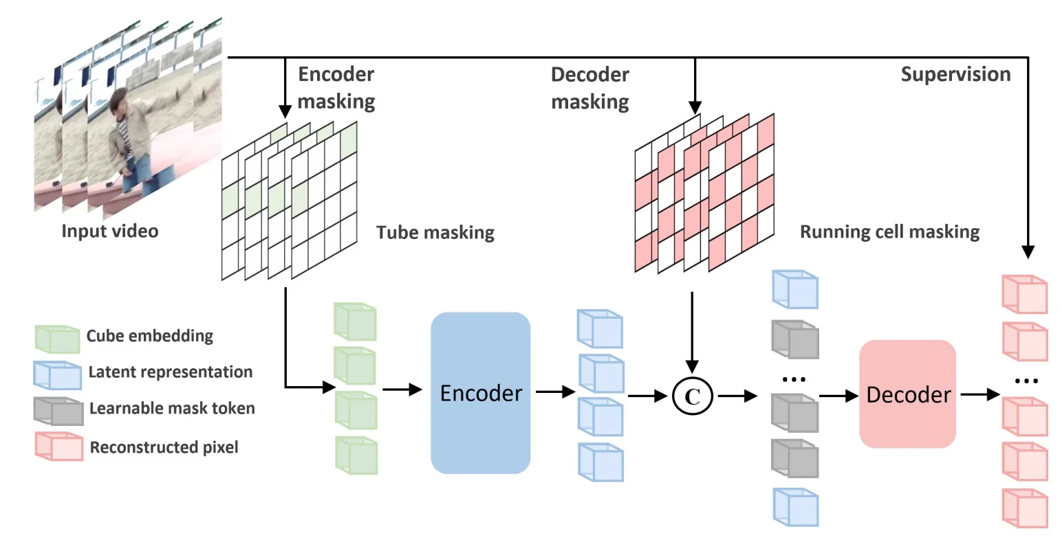
Method
Preliminaries and notation A temporally subsampled clip \(I \in \mathbb {R}^{T\times H\times W\times 3}\) is divided into spatiotemporal cubes of size \(k\times P\times P\) (e.g., \(2\times 16 \times 16\)). Each cube is linearly embedded into \(\mathbb {R}^D\), yielding \[ N = \tfrac {T}{k}\cdot \tfrac {H}{P}\cdot \tfrac {W}{P} \] tokens. An encoder tube mask \(M_e\) with ratio \(\rho ^e \in [0.9,0.95]\) is sampled on the spatial grid and broadcast over time. Let \(V\) denote visible positions and \(E\) the encoder-masked set. The encoder processes only visible tokens: \begin {equation} Z = \Phi _{\mathrm {enc}}(\{T_i\}_{i \in V}). \label {eq:chapter24_videomaev2_enc} \end {equation}
Dual masking: decoder-side selection A decoder mask \(M_d\) with ratio \(\rho ^d\) selects which cubes to reconstruct. The default is running-cell masking, which ensures spatiotemporal coverage without degenerate patterns (e.g., whole frames). Let \(D\) be decoder-visible positions. The decoder input is: \begin {equation} U = [Z \cup \{M_i\}_{i \in D}], \qquad \hat I = \Phi _{\mathrm {dec}}(U). \label {eq:chapter24_videomaev2_decinput} \end {equation}
Loss on encoder-invisible & decoder-visible cubes Reconstruction loss is applied only to tokens that were invisible to the encoder but selected for reconstruction by the decoder: \begin {equation} \mathcal {L}_{\mathrm {DM}} \;=\; \frac {1}{|E \cap D|}\sum _{i \in E \cap D} \|I_i - \hat I_i\|_2^2, \label {eq:chapter24_videomaev2_loss} \end {equation} where \(E\) is the set of encoder-masked positions and \(D\) the set of decoder-visible positions. The loss is restricted to \(E\cap D\) to avoid information leakage.
Running-cell masking for decoder supervision Goal. Make the decoder cheap but informative: at each iteration it reconstructs only a small, contiguous 3D block of tokens (a cell) rather than every masked token.
Setup (single knob = cell size). After cubeization the token grid has shape \( (N_t,N_h,N_w)=\big (\tfrac {T}{k},\,\tfrac {H}{P},\,\tfrac {W}{P}\big ) \) with indices \((t',x,y)\). Choose a cell size \((C_t,C_h,C_w)\). The decoder keep-rate (fraction of tokens it will process in a step) is simply the cell-to-grid volume ratio: \[ 1-\rho ^d \;\approx \; \frac {|D_s|}{N} = \frac {C_t\,C_h\,C_w}{N_t\,N_h\,N_w},\qquad N=N_tN_hN_w. \] Example. If \((N_t,N_h,N_w)=(8,14,14)\) then a cell \((4,7,7)\) yields \(196/1568\approx 12.5\%\) keep-rate; to target \(\approx 50\%\) use a larger cell, e.g., \((6,12,12)\) giving \(864/1568\approx 55\%\).
Selection rule (what the decoder sees). At training step \(s\), pick a cell origin \((t_0,x_0,y_0)\) and define the decoder-visible set \[ D_s=\big \{(t',x,y):\; t_0 \le t' < t_0{+}C_t,\; x_0 \le x < x_0{+}C_h,\; y_0 \le y < y_0{+}C_w\big \}. \] Placement. Random (default): sample \((t_0,x_0,y_0)\) uniformly—each step hits a different region with high probability. Strided (alt.): move with strides \((S_t,S_h,S_w)\) and wrap for deterministic coverage.
What happens next (mechanics). The decoder input consists of (i) encoder features from the few visible tokens and (ii) learned mask tokens only at indices in \(D_s\). The decoder predicts pixels only for \(D_s\), and the loss is computed strictly on the intersection with the encoder-masked set: \[ \mathcal {L} \;=\; \frac {1}{|E\cap D_s|}\sum _{i\in E\cap D_s}\|I_i-\hat I_i\|_2^2, \] so tokens seen by the encoder (\(V\)) never contribute to the loss even if they lie in \(D_s\).
Why this design works.
- Coherent supervision. A contiguous 3D cell provides local space–time context, which is a stronger signal than isolated random tokens.
- Even coverage over training. Random (or strided) placement prevents target clustering and ensures every region is eventually supervised.
- Predictable efficiency. Decoder cost scales with \(|D_s|\) (i.e., with \(1-\rho ^d\)), giving a simple, explicit trade-off via \((C_t,C_h,C_w)\).
- Leakage-free objective. Restricting the loss to \(E\cap D_s\) preserves the MAE principle and blocks copying from encoder-visible tokens.
Algorithmic flow (pseudo code)
# VideoMAEv2 pre-training step (schematic)
# I: clip [T,H,W,3]; rho_e: encoder mask ratio; rho_d: decoder mask ratio
# Phi_emb: cube embedding; Enc: ViT encoder; Dec: lightweight ViT decoder

def step(I, rho_e=0.9, rho_d=0.5):
    X = Phi_emb(cubeify(I))                 # tokens T_1..T_N
    Ve, Ee = tube_mask_indices(N=X.shape[0], ratio=rho_e)  # visible / masked for encoder
    Z = Enc(X[Ve])                          # encode only visible tokens
    D = running_cell_mask_indices(N=X.shape[0], ratio=rho_d)  # decoder-kept positions
    masked_tokens = learnable_mask_tokens(indexes=D)
    U = concat(Z, masked_tokens)            # decoder sequence
    I_hat = Dec(U)                          # predictions at positions in D
    idx = intersect(Ee, D)                  # loss only on encoder-invisible & decoder-visible
    return mse(I_hat[idx], targets(I)[idx]) / len(idx)
Architecture and Implementation Details
- Encoders. ViT-B/L/H and the billion-parameter ViT-g are used as encoders with joint space–time attention.
- Decoder. A lightweight ViT (e.g., \(4\) blocks) with narrower width reconstructs pixel targets from \(U\); masking the decoder reduces its token length to \((1{-}\rho ^{d})N\).
- Encoder masking (\(\rho ^{e}\)). High-ratio tube masking as in VideoMAE (\(90\)–\(95\%\)).
- Decoder masking (\(\rho ^{d}\)). Running cell masking with default \(\rho ^{d}\!=\!0.5\) unless otherwise stated; alternatives (frame masking, random masking) are evaluated in ablations.
-
Pre-training corpora.
- UnlabeledHybrid (UH, \(\sim \)1.35M clips): mixed, de-duplicated web video sources used without labels for self-supervised pre-training.
- LabeledHybrid (LH, K710-aligned): same mixture but with labels for optional progressive post-pre-training before downstream fine-tuning.
- IG-uncurated: \(\sim \)1M Instagram videos without labels (used in MAE-ST baselines for scale comparison).
-
Downstream datasets (names \(\rightarrow \) shorthand).
- Kinetics-400 \(\rightarrow \) K400: \(\sim \)240k YouTube clips, 400 actions; appearance-centric.
- Kinetics-600 \(\rightarrow \) K600: \(\sim \)480–500k clips, 600 actions (expanded Kinetics).
- Kinetics-700 \(\rightarrow \) K700: \(\sim \)650k clips, 700 actions.
- Kinetics-710 \(\rightarrow \) K710: curated 710-class labeled mix used for progressive post-pre-train in V2.
- Something-Something V2 \(\rightarrow \) SSv2: \(\sim \)169k clips of object-centric interactions; motion-centric.
- Something-Something V1 \(\rightarrow \) SSv1: earlier SSv2 release used in some SOTA tables.
- AVA v2.2 \(\rightarrow \) AVA: spatio-temporal action detection (1s annotations) on movie clips; report mAP.
- AVA-Kinetics \(\rightarrow \) AVA-K: long-form detection benchmark combining AVA with Kinetics for training/testing.
- THUMOS14: temporal action detection on untrimmed videos; report mAP at multiple IoU thresholds.
- FineAction: temporal detection dataset of fine-grained actions; report mAP.
-
Input & sampling.
- Clip shape: typically \(16\times 224^2\); temporal stride \(\tau \in \{2,4\}\) during pre-train.
- Fine-tune sampling: TSN-style sparse sampling on SSv2; dense/multi-view on Kinetics (K400/K600/K700/K710).
- Inference views: SSv2: \(2\times 3\) (temporal \(\times \) spatial); Kinetics: \(5\times 3\) (unless otherwise noted in SOTA tables).
-
Optimization schedules.
- Pre-train: 1200 epochs on 64 GPUs for UH/LH; SSv2 ablations commonly at 800 epochs.
- Masking: encoder tube masking \(\rho ^{e}\in [0.90,0.95]\); decoder running-cell masking with keep-rate \(1-\rho ^{d}\approx 0.25\sim 0.50\) (per ablation).
- Targets & loss: per-cube pixel normalization; MSE on \(E\cap D\) (encoder-invisible & decoder-visible).
Experiments and Ablation
| Decoder Masking | \(\rho ^{d}\) | Top-1 | FLOPs |
|---|---|---|---|
| None | 0% | 70.28 | 35.48G |
| Frame | 50% | 69.76 | 25.87G |
| Random | 50% | 64.87 | 25.87G |
| Running cell\(^{1}\) | 50% | 66.74 | 25.87G |
| Running cell\(^{2}\) | 25% | 70.22 | 31.63G |
| Running cell\(^{2}\) | 50% | 70.15 | 25.87G |
| Running cell\(^{2}\) | 75% | 70.01 | 21.06G |
\(^{1}\)Loss over all decoder outputs. \(^{2}\)Loss over decoder outputs invisible to the encoder.
| Masking | Backbone | Pre-training dataset | FLOPs | Mems | Time | Speedup | Top-1 |
| Encoder masking | ViT-B | Sth-Sth V2 | 35.48G | 631M | 28.4h | - | 70.28 |
| Dual masking | ViT-B | Sth-Sth V2 | 25.87G | 328M | 15.9h | 1.79\(\times \) | 70.15 |
| Encoder masking | ViT-g | UnlabeledHybrid | 263.93G | 1753M | 356h\(^{\dagger }\) | - | - |
| Dual masking | ViT-g | UnlabeledHybrid | 241.61G | 1050M | 241h | 1.48\(\times \) | 77.00 |
| Method | Pre-train data | Data size | Epoch | ViT-B | ViT-L | ViT-H / ViT-g |
| MAE-ST [57] | Kinetics400 | 0.24M | 1600 | - | 72.1 | 74.1 |
| MAE-ST [57] | Kinetics700 | 0.55M | 1600 | - | 73.6 | 75.5 |
| VideoMAE V1 [42] | Sth-Sth V2 | 0.17M | 2400 | 70.8 | 74.3 | 74.8 |
| VideoMAE V2 | UnlabeledHybrid | 1.35M | 1200 | 71.2 (69.5) | 75.7 (74.0) | 76.8 / 77.0 (75.5 / 75.7) |
Progressive pre-training (K710)
State of the art (selected benchmarks)
| Method | Top 1 | Top 5 | Views | TFLOPs |
| I3D NL [8] | 77.7 | 93.3 | \(10 \times 3\) | 10.77 |
| TDN [51] | 79.4 | 94.4 | \(10 \times 3\) | 5.94 |
| SlowFast R101–NL [45] | 79.8 | 93.9 | \(10 \times 3\) | 7.02 |
| TimeSformer–L [11] | 80.7 | 94.7 | \(1 \times 3\) | 7.14 |
| MTV–B (\(320^2\)) [58] | 82.4 | 95.2 | \(4 \times 3\) | 11.16 |
| Video Swin–L (\(384^2\)) [53] | 84.9 | 96.7 | \(10 \times 5\) | 105.35 |
| ViViT–L FE [12] | 81.7 | 93.8 | \(1 \times 3\) | 11.94 |
| MViTv2–L (\(312^2\)) [15] | 86.1 | 97.0 | \(40 \times 3\) | 42.42 |
| MaskFeat [48] | 87.0 | 97.4 | \(4 \times 3\) | 45.48 |
| MAE–ST [57] | 86.8 | 97.2 | \(4 \times 3\) | 25.05 |
| VideoMAE [42] | 86.6 | 97.1 | \(5 \times 3\) | 17.88 |
| VideoMAE V2–H [43] | 88.6 | 97.9 | \(5 \times 3\) | 17.88 |
| VideoMAE V2–g [43] | 88.5 | 98.1 | \(5 \times 3\) | 38.16 |
| VideoMAE V2–g (\(64 \times 266^2\)) [43] | 90.0 | 98.4 | \(2 \times 3\) | 160.30 |
| Method | Top 1 | Top 5 | Views | TFLOPs |
| SlowFast R101–NL [45] | 81.8 | 95.1 | \(10 \times 3\) | 7.02 |
| TimeSformer–L [11] | 82.2 | 95.6 | \(1 \times 3\) | 7.14 |
| MTV–B (\(320^2\)) [58] | 84.0 | 96.2 | \(4 \times 3\) | 11.16 |
| ViViT–L FE [12] | 82.9 | 94.6 | \(1 \times 3\) | 11.94 |
| MViTv2–L (\(352^2\)) [15] | 87.9 | 97.9 | \(40 \times 3\) | 45.48 |
| MaskFeat [48] | 86.4 | 97.4 | \(1 \times 10\) | 3.77 |
| VideoMAE V2–H [43] | 88.3 | 98.1 | \(5 \times 3\) | 17.88 |
| VideoMAE V2–g [43] | 88.8 | 98.2 | \(5 \times 3\) | 38.16 |
| VideoMAE V2–g (\(64 \times 266^2\)) [43] | 89.9 | 98.5 | \(2 \times 3\) | 160.30 |
| Method | Top 1 | Top 5 |
| SlowFast [45] | 63.1 | 87.6 |
| TEINet [49] | 66.5 | – |
| TEA [59] | 65.1 | 89.9 |
| TDN [51] | 69.6 | 92.2 |
| TimeSformer–L [11] | 62.4 | – |
| MFormer–HR [52] | 68.1 | 91.2 |
| ViViT–L FE [12] | 65.9 | 89.9 |
| Video Swin–B [53] | 69.6 | 92.7 |
| MViTv2–B [15] | 72.1 | 93.4 |
| MTV–B [58] | 67.6 | 90.1 |
| BEVT [55] | 70.6 | – |
| VIMPAC [54] | 68.1 | – |
| UniFormer [60] | 71.2 | 92.8 |
| MaskFeat [48] | 75.0 | 95.0 |
| MAE–ST [57] | 75.5 | 95.0 |
| VideoMAE [42] | 75.4 | 95.2 |
| VideoMAE V2–H [43] | 76.8 | 95.8 |
| VideoMAE V2–g [43] | 77.0 | 95.9 |
Limitations and Future Work
- Pixel supervision bottleneck. Reconstruction remains anchored to low-level RGB fidelity. While effective for generic features, it underemphasizes semantic abstraction and long-range motion cues—exactly where large-scale video understanding needs stronger supervision.
- Decoder still tied to reconstruction. Even with dual masking, the decoder only learns to inpaint pixels. This constrains learning to local texture statistics rather than global semantics.
- Scaling trade-offs. Very large encoders (ViT-H, ViT-g) show diminishing gains on recognition benchmarks, suggesting that simply scaling model size without enriching the training signal plateaus.
- Domain gaps. Hybrid pretraining datasets balance appearance and motion imperfectly. Representations trained purely on RGB inputs may not capture compositional or multimodal cues needed in downstream tasks.
Future directions (path toward distillation and beyond)
- From pixels to features (MVD). A natural next step is to replace pixel-level regression with feature-level targets, as in Masked Video Distillation [691]. Teacher encoders (e.g., image- or video-pretrained transformers) provide richer supervisory signals on masked regions, injecting semantics and motion awareness absent from raw RGB.
- Dynamic decoder supervision. Beyond fixed cells, learned policies for decoder token selection or adaptive sparsification can focus computation on informative spatio-temporal regions, preserving efficiency while scaling to longer clips.
- Multi-granular objectives. Combining reconstruction with motion-sensitive or perceptual losses could better capture dynamics, addressing VideoMAEv2’s limitation to mostly static appearance cues.
- Cross-modal grounding. Incorporating audio or text alignment, as explored in later video–language pretraining work, may reduce ambiguity and enable open-vocabulary recognition and retrieval.
- Stress-testing benchmarks. Moving beyond short-clip classification toward long-form reasoning, dense temporal localization, and open-vocabulary tasks will better expose the strengths and weaknesses of masked video pretraining methods.
Enrichment 24.6.3: MVD: Masked Video Distillation
Scope and positioning Background. Masked Image Modeling (MIM) and Masked Video Modeling (MVM) are self-supervised pretraining paradigms that hide a large subset of patches and train a model to reconstruct the hidden content. For videos, VideoMAE [642] applies very high tube masking (typically \(90\)–\(95\%\)) and asks a ViT to reconstruct raw pixels in the masked spatio-temporal cubes using a lightweight decoder, yielding strong baselines but still supervising at the pixel level. MVD [691] rethinks the reconstruction target: instead of pixels, the student predicts high-level features produced by frozen, pretrained teacher encoders. Two complementary teachers are used: an image teacher (MIM-pretrained on images; strong spatial semantics) and a video teacher (MVM-pretrained on videos; motion-aware spatio-temporal semantics). The student video encoder sees only the visible tokens of a tube-masked clip and, through shallow decoders with Smooth-\(\ell _1\) regression, learns to reconstruct the teacher’s features at the masked positions. Empirically, this masked feature modeling yields consistent gains over pixel reconstruction (e.g., VideoMAE) on recognition and spatio-temporal detection benchmarks [691].
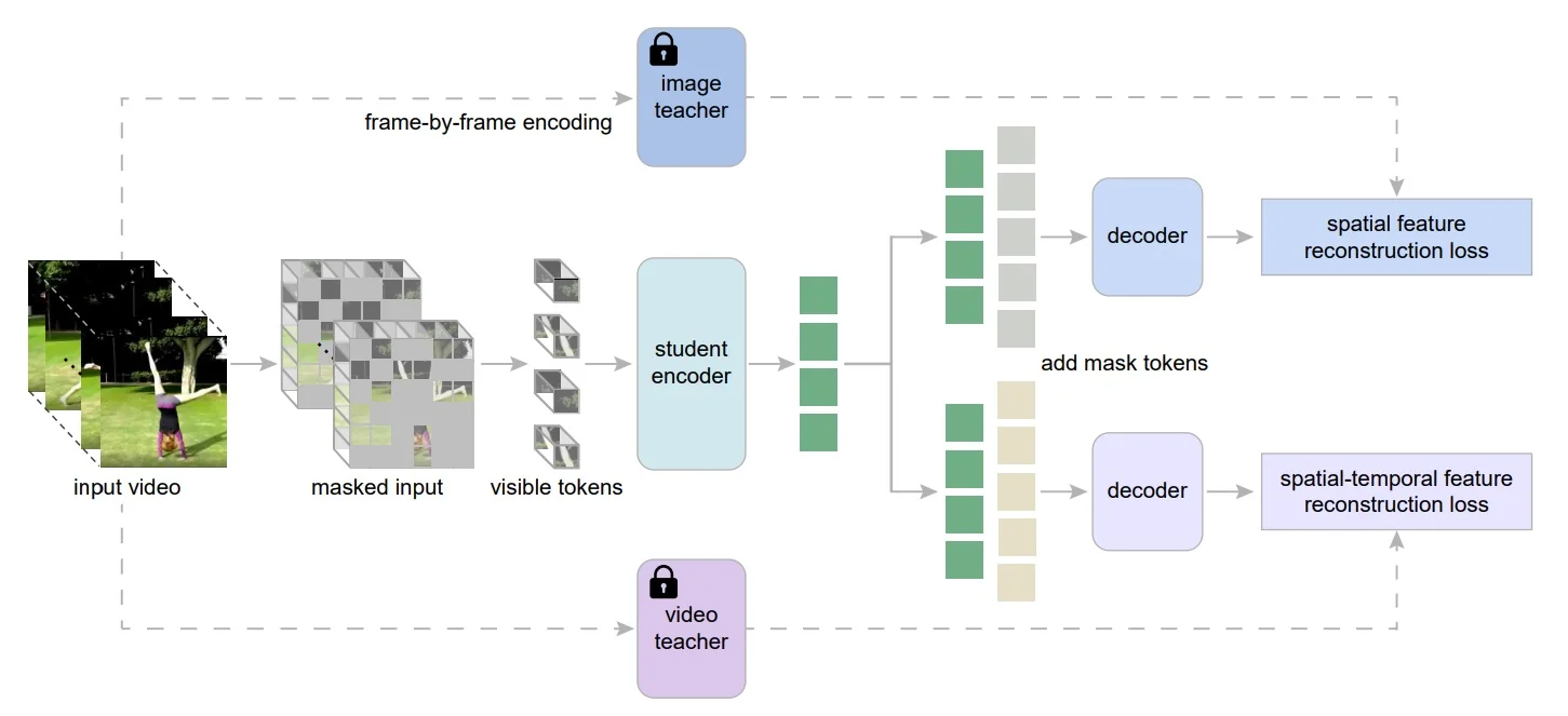
Motivation
Limits of pixel-level MVM (VideoMAE). Pixel reconstruction under MVM is affected by video temporal redundancy: adjacent frames are highly similar, so a model can fill in masked pixels by copying or interpolating from nearby context without forming strong high-level abstractions. Even with VideoMAE’s very high masking ratio and tube masking, the supervision remains low level and noisy, which can encourage shortcut solutions and yield features that transfer suboptimally on action-centric tasks [642, 691].
From pixels to features: cleaner targets and inductive bias. MVD [691] replaces RGB regression with feature regression against targets from powerful self-supervised teachers. High-level targets suppress nuisance variation (e.g., lighting, small pixel noise) and encode semantics that downstream tasks care about, providing a cleaner learning signal and a better inductive bias than raw pixels. Practically, the student predicts masked-patch features produced by frozen teachers while only encoding the visible tokens, preserving the compute advantages of masked modeling.
Why two teachers: complementary spatial and temporal cues. Image teachers (MIM-pretrained) specialize in spatial appearance and yield features that are highly similar across neighboring frames; video teachers (MVM-pretrained) encode temporal dynamics and produce frame features whose similarity decays with temporal distance. MVD leverages this complementarity through spatial–temporal co-teaching: two independent decoders regress to the image-teacher and video-teacher targets, respectively, so the shared student is simultaneously pressured to preserve strong spatial semantics and temporal sensitivity. This design helps a single student excel on both appearance-biased datasets (e.g., Kinetics-400) and motion-centric datasets (e.g., Something-Something V2), explaining the observed gains over VideoMAE across settings [691].
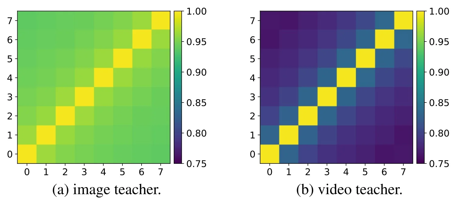
Method
Preliminaries: masked feature modeling Let \(X_{\mbox{vid}}\in \mathbb {R}^{T\times H\times W\times 3}\) be a video, partitioned into non-overlapping spatio-temporal patches (tubelets). After linear patch embedding, a subset \(\mathcal {M}\) of tokens is masked (tube masking) and dropped from the encoder input; the visible tokens \(X_{\mbox{vis}}\) are encoded by a student transformer \(f\). A shallow transformer decoder \(g\) receives \(\operatorname {concat}(f(X_{\mbox{vis}}),T_m)\), where \(T_m\) are learnable mask tokens, and predicts outputs \(Y\) for all token positions: \begin {equation} Y \;=\; g\!\big (\operatorname {concat}(f(X_{\mbox{vis}}), T_m)\big ) \label {eq:chapter24_mvd_forward} \end {equation} Given a target feature generator \(h\) that maps each masked patch \(X^{(p)}\) to a target feature \(h(X^{(p)})\), the masked feature modeling objective is \begin {equation} \mathcal {L}_{\mbox{mfm}}(h) \;=\; \frac {1}{|\mathcal {M}|}\sum _{p\in \mathcal {M}} D\!\left (Y^{(p)},\, h\!\left (X^{(p)}\right )\right ) \label {eq:chapter24_mvd_mfm} \end {equation} where \(D\) is a distance measure; MVD adopts Smooth-\(\ell _1\) (Huber) loss [691].
Teacher targets MVD instantiates \(h\) as frozen self-supervised teacher encoders:
- Spatial (image) targets. An image-teacher encoder \(h_{\mbox{img}}\) pretrained by masked image modeling (e.g., MAE on IN1K) encodes each frame independently to provide appearance-focused features.
- Spatio-temporal (video) targets. A video-teacher encoder \(h_{\mbox{vid}}\) pretrained by masked video modeling (e.g., VideoMAE on K400) encodes clips to provide motion-aware features.
A \(2\times 16\times 16\) 3D patch for the video student corresponds to two \(16\times 16\) 2D patches for the image teacher; MVD predicts the front slice’s spatial target to reduce the prediction head size [691].
Spatial–temporal co-teaching To fuse complementary supervision, MVD attaches two decoders \(g_{\mbox{img}}\) and \(g_{\mbox{vid}}\) (same architecture, independent parameters) to the shared student features \(f(X_{\mbox{vis}})\): \begin {equation} \mathcal {L}_{\mbox{MVD}} \;=\; \lambda _1\,\mathcal {L}_{\mbox{mfm}}(h_{\mbox{img}}) \;+\; \lambda _2\,\mathcal {L}_{\mbox{mfm}}(h_{\mbox{vid}}) \label {eq:chapter24_mvd_total} \end {equation} with scalars \(\lambda _1,\lambda _2\) balancing the two teachers. This objective compels the student to reconstruct masked tokens so that both image-like and video-like semantics are preserved, strengthening spatial discrimination and temporal sensitivity simultaneously [691].
Algorithmic view The official pseudocode (PyTorch style) is reproduced verbatim (line breaks adapted) in Enrichment 24.6.3. Notation: \(f\) student, \(g_{\mbox{img}}/g_{\mbox{vid}}\) decoders, \(T_m\) mask tokens, \(h_{\mbox{img}}/h_{\mbox{vid}}\) frozen teachers, \(m\) binary mask.
# Algorithm 1 Pseudocode of MVD in PyTorch style (from \cite{wang2023_mvd})
# f: student encoder
# g_img: decoder for reconstructing spatial features
# g_vid: decoder for reconstructing spatial-temporal features
# t_m: learnable mask tokens
# h_img: image teacher model
# h_vid: video teacher model
for x, m in loader:  # x: video data, m: mask
    x_pe = patch_emb(x)               # patch embedding of input
    x_vis = mask_select(x_pe, 1 - m)  # masking tokens
    q_vis = f(x_vis)                  # visible local patch features
    # reconstruction of target features
    p_img = g_img(concat(q_vis, t_m))
    p_vid = g_vid(concat(q_vis, t_m))
    # compute target features with teacher models
    k_img = h_img(x)  # target spatial features
    k_vid = h_vid(x)  # target spatial-temporal features
    # compute reconstruction loss
    loss_img = smooth_L1_loss(p_img * m, k_img * m)
    loss_vid = smooth_L1_loss(p_vid * m, k_vid * m)
    loss = lambda_1 * loss_img + lambda_2 * loss_vid
    loss.backward()
    optimizer.step()  # optimizer update
Intuition and failure-mode mitigation
- Richer supervision than pixels. High-level targets abstract away nuisance low-level variability, biasing the student toward semantics that transfer better across datasets and tasks.
- Masking as structured context removal. Tube masking removes entire spatio-temporal tubes, forcing the student to hallucinate both appearance and motion content consistent with teacher features rather than raw RGB.
- Decoupled decoders avoid interference. Separate heads let each teacher specialize its prediction space without compromising the other, while gradients meet only in the shared student.
Architecture and implementation details
Backbone and tokenization A vanilla ViT encoder (ViT-S/B/L/H) serves as \(f\). 3D patch embedding with size \(2\times 16\times 16\) produces \(T/2\times H/16\times W/16\) tokens. During pretraining, a high masking ratio (e.g., \(90\%\)) with tube masking is applied; only visible tokens are encoded [691, 642].
Attention Joint spatio-temporal self-attention is applied within each encoder block over the visible token sequence. Learned mask tokens \(T_m\) are concatenated with \(f(X_{\mbox{vis}})\) before each decoder.
Decoders and objectives Two shallow transformer decoders (a few layers) plus linear heads predict teacher features at masked positions. Smooth-\(\ell _1\) regression is used for both branches; the loss is computed only on masked tokens via elementwise masking, as in (24.18)–(24.19) [691].
Pretraining schedules Teachers: MAE image-teacher on IN1K (e.g., 1600 epochs), VideoMAE video-teacher on K400 (e.g., 1600 epochs). Student: distilled on K400 for 400 epochs by default (800 in some settings), AdamW optimizer, clip length \(T{=}16\) for pretrain and finetune [691].
Experiments and ablation
Main results and efficiency On SSv2, MVD dominates the accuracy–compute frontier relative to supervised and self-supervised peers (see below figure). Relative to VideoMAE [642], MVD delivers consistent gains across model scales with substantially fewer pretraining epochs [691].
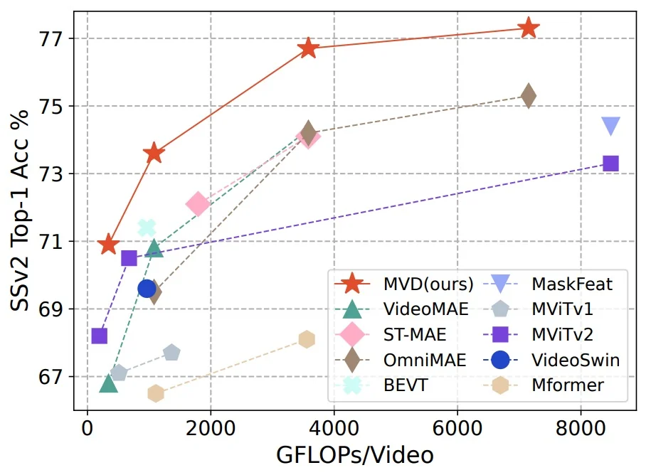
Gains over VideoMAE across scales
| Student | Teacher | K400 (VideoMAE) | K400 (MVD) | SSv2 (VideoMAE) | SSv2 (MVD) |
|---|---|---|---|---|---|
| ViT-S | ViT-B | 79.0 | 80.6 | 66.4 | 70.7 |
| ViT-S | ViT-L | 79.0 | 81.0 | 66.4 | 70.9 |
| ViT-B | ViT-B | 81.5 | 82.7 | 69.7 | 72.5 |
| ViT-B | ViT-L | 81.5 | 83.4 | 69.7 | 73.7 |
| ViT-L | ViT-L | 85.2 | 86.0 | 74.0 | 76.1 |
| Student | Image | Video | K400 top-1 (%) | SSv2 top-1 (%) |
|---|---|---|---|---|
| ViT-S | ✓ | ✗ | 80.4 | 69.4 |
| ViT-S | ✗ | ✓ | 80.1 | 70.0 |
| ViT-S | ✓ | ✓ | 80.6 | 70.7 |
| ViT-B | ✓ | ✗ | 82.3 | 71.4 |
| ViT-B | ✗ | ✓ | 82.1 | 71.8 |
| ViT-B | ✓ | ✓ | 82.7 | 72.5 |
Gains over VideoMAE across scales
| Student | Teacher | K400 (VideoMAE) | K400 (MVD) | SSv2 (VideoMAE) | SSv2 (MVD) |
|---|---|---|---|---|---|
| ViT-S | ViT-B | 79.0 | 80.6 | 66.4 | 70.7 |
| ViT-S | ViT-L | 79.0 | 81.0 | 66.4 | 70.9 |
| ViT-B | ViT-B | 81.5 | 82.7 | 69.7 | 72.5 |
| ViT-B | ViT-L | 81.5 | 83.4 | 69.7 | 73.7 |
| ViT-L | ViT-L | 85.2 | 86.0 | 74.0 | 76.1 |
End-to-end comparisons Selections from [691] are reproduced below for completeness. Methods cited include supervised baselines and self-supervised contemporaries such as ST-MAE [159], OmniMAE [180], BEVT [690], MaskFeat [710], MViTv2 [354], VideoSwin [396], TimeSformer [41], ViViT [16], SlowFast [160], NL I3D [698], ip-CSN [649], X3D [155], MViTv1 [152], UniFormer [347], and Mformer [490]. All numbers and settings match the paper’s tables.
| Method | Extra data | top-1 | top-5 | GFLOPs / Param |
|---|---|---|---|---|
| NL I3D R101 [80] | – | 77.3 | 93.3 | \(359{\times }30\) / 62 |
| ip-CSN-152 [56] | – | 77.8 | 92.8 | \(109{\times }30\) / 33 |
| SlowFast NL [45] | – | 79.8 | 93.9 | \(234{\times }30\) / 60 |
| X3D-XL [81] | – | 79.1 | 93.9 | \(48{\times }30\) / 11 |
| MViTv1-B [14] | – | 80.2 | 94.4 | \(170{\times }5\) / 37 |
| VideoSwin-B [53] | IN-1K | 80.6 | 94.6 | \(282{\times }12\) / 88 |
| Uniformer-B [60] | IN-1K | 83.0 | 95.4 | \(259{\times }12\) / 50 |
| TimeSformer [11] | IN-21K | 80.7 | 94.7 | \(2380{\times }3\) / 121 |
| Mformer-B [82] | IN-21K | 79.7 | 94.2 | \(370{\times }30\) / 109 |
| Mformer-L [82] | IN-21K | 80.2 | 94.8 | \(1185{\times }30\) / 382 |
| ViViT-L FE [12] | IN-21K | 81.7 | 93.8 | \(3980{\times }3\) / N/A |
| VideoSwin-L [53] | IN-21K | 83.1 | 95.9 | \(604{\times }12\) / 197 |
| VIMPAC ViT-L [54] | HowTo100M | 77.4 | N/A | N/A\(\times \)30 / 307 |
| BEVT Swin-B [55] | IN-1K | 81.1 | N/A | \(282{\times }12\) / 88 |
| MaskFeat MViT-S [48] | – | 82.2 | 95.1 | \(71{\times }10\) / 36 |
| VideoMAE ViT-S [42] | – | 79.0 | 93.8 | \(57{\times }15\) / 22 |
| VideoMAE ViT-B [42] | – | 81.5 | 95.1 | \(180{\times }15\) / 87 |
| VideoMAE ViT-L [42] | – | 85.2 | 96.8 | \(597{\times }15\) / 305 |
| VideoMAE ViT-H [42] | – | 86.6 | 97.1 | \(1192{\times }15\) / 633 |
| ST-MAE ViT-B [57] | – | 81.3 | 94.9 | \(180{\times }21\) / 87 |
| ST-MAE ViT-L [57] | – | 84.8 | 96.2 | \(598{\times }21\) / 304 |
| ST-MAE ViT-H [57] | – | 85.1 | 96.6 | \(1193{\times }21\) / 632 |
| OmniMAE ViT-B [79] | IN-1K | 80.8 | N/A | \(180{\times }15\) / 87 |
| OmniMAE ViT-L [79] | IN-1K+SSv2 | 84.0 | N/A | \(597{\times }15\) / 305 |
| OmniMAE ViT-H [79] | IN-1K+SSv2 | 84.8 | N/A | \(1192{\times }15\) / 633 |
| MVD-S (Teacher-B) [44] | IN-1K | 80.6 | 94.7 | \(57{\times }15\) / 22 |
| MVD-S (Teacher-L) [44] | IN-1K | 81.0 | 94.8 | \(57{\times }15\) / 22 |
| MVD-B (Teacher-B) [44] | IN-1K | 82.7 | 95.4 | \(180{\times }15\) / 87 |
| MVD-B (Teacher-L) [44] | IN-1K | 83.4 | 95.8 | \(180{\times }15\) / 87 |
| MVD-L (Teacher-L) [44] | IN-1K | 86.0 | 96.9 | \(597{\times }15\) / 305 |
| MVD-L (Teacher-L)\(^\dagger \) [44] | IN-1K | 86.4 | 97.0 | \(597{\times }15\) / 305 |
| MVD-H (Teacher-H)\(^\dagger \) [44] | IN-1K | 87.2 | 97.4 | \(1192{\times }15\) / 633 |
| Method | Extra data | top-1 | GFLOPs | Param |
|---|---|---|---|---|
supervised |
||||
| SlowFast R101 [45] | K400 | 63.1 | \(106{\times }3\) | 53 |
| TSM-RGB R50 [62] | IN-1K | 63.3 | \(62{\times }6\) | 24 |
| TAM R50 [83] | IN-1K | 66.0 | \(99{\times }6\) | 51 |
| TDN R101 [51] | IN-1K | 69.6 | \(198{\times }3\) | 88 |
| MViTv1-B [14] | – | 67.7 | \(455{\times }3\) | 37 |
| MViTv2-B [15] | K400 | 70.5 | \(225{\times }3\) | 51 |
| UniFormer-B [60] | K400 | 71.2 | \(259{\times }3\) | 50 |
| TimeSformer-HR [11] | IN-21K | 62.5 | \(1703{\times }3\) | 121 |
| ViViT-L FE [12] | IN-21K+K400 | 65.9 | \(995{\times }12\) | N/A |
| Mformer-B [82] | IN-21K+K400 | 66.5 | \(370{\times }3\) | 109 |
| Mformer-L [82] | IN-21K+K400 | 68.1 | \(1185{\times }3\) | 382 |
| VideoSwin-B [53] | IN-21K+K400 | 69.6 | \(321{\times }3\) | 88 |
| MViTv2-L [15] | IN-21K+K400 | 73.3 | \(2828{\times }3\) | 213 |
self-supervised |
||||
| VIMPAC ViT-L [54] | HowTo100M | 68.1 | N/A\(\times \)30 | 307 |
| BEVT Swin-B [55] | IN-1K+K400 | 71.4 | \(321{\times }3\) | 88 |
| MaskFeat MViT-L [48] | K400 | 74.4 | \(2828{\times }3\) | 218 |
| VideoMAE ViT-S [42] | K400 | 66.4 | \(57{\times }6\) | 22 |
| VideoMAE ViT-S [42] | – | 66.8 | \(57{\times }6\) | 22 |
| VideoMAE ViT-B [42] | K400 | 69.7 | \(180{\times }6\) | 87 |
| VideoMAE ViT-B [42] | – | 70.8 | \(180{\times }6\) | 87 |
| VideoMAE ViT-L [42] | K400 | 74.0 | \(597{\times }6\) | 305 |
| VideoMAE ViT-L [42] | – | 74.3 | \(597{\times }6\) | 305 |
| ST-MAE ViT-L [57] | K400 | 72.1 | \(598{\times }3\) | 304 |
| ST-MAE ViT-H [57] | K400 | 74.1 | \(1193{\times }3\) | 632 |
| OmniMAE ViT-B [79] | IN-1K | 69.5 | \(180{\times }6\) | 87 |
| OmniMAE ViT-B [79] | IN-1K+K400 | 69.0 | \(180{\times }6\) | 87 |
| OmniMAE ViT-L [79] | IN-1K | 74.2 | \(597{\times }6\) | 305 |
| OmniMAE ViT-H [79] | IN-1K | 75.3 | \(1192{\times }6\) | 632 |
| MVD-S (Teacher-B) [44] | IN-1K+K400 | 70.7 | \(57{\times }6\) | 22 |
| MVD-S (Teacher-L) [44] | IN-1K+K400 | 70.9 | \(57{\times }6\) | 22 |
| MVD-B (Teacher-B) [44] | IN-1K+K400 | 72.5 | \(180{\times }6\) | 87 |
| MVD-B (Teacher-L) [44] | IN-1K+K400 | 73.7 | \(180{\times }6\) | 87 |
| MVD-L (Teacher-L) [44] | IN-1K+K400 | 76.1 | \(597{\times }6\) | 305 |
| MVD-L (Teacher-L)\(^\dagger \) [44] | IN-1K+K400 | 76.7 | \(597{\times }6\) | 305 |
| MVD-H (Teacher-H)\(^\dagger \) [44] | IN-1K+K400 | 77.3 | \(1192{\times }6\) | 633 |
| Method | Extra data | Extra labels | mAP | GFLOPs |
|---|---|---|---|---|
| SlowFast R101 [45] | K400 | ✓ | 23.8 | 138 |
| MViTv2-B [15] | K400 | ✓ | 29.0 | 225 |
| MViTv2-L [15] | IN-21K+K700 | ✓ | 34.4 | 2828 |
| MaskFeat MViT-L [48] | K400 | ✓ | 37.5 | 2828 |
| VideoMAE ViT-B [42] | K400 | ✗ | 26.7 | 180 |
| VideoMAE ViT-B [42] | K400 | ✓ | 31.8 | 180 |
| VideoMAE ViT-L [42] | K400 | ✗ | 34.3 | 597 |
| VideoMAE ViT-L [42] | K400 | ✓ | 37.0 | 597 |
| VideoMAE ViT-H [42] | K400 | ✗ | 36.5 | 1192 |
| VideoMAE ViT-H [42] | K400 | ✓ | 39.5 | 1192 |
| ST-MAE ViT-L [57] | K400 | ✓ | 35.7 | 598 |
| ST-MAE ViT-H [57] | K400 | ✓ | 36.2 | 1193 |
| MVD-B (Teacher-B) [44] | IN-1K+K400 | ✗ | 29.3 | 180 |
| MVD-B (Teacher-B) [44] | IN-1K+K400 | ✓ | 33.6 | 180 |
| MVD-B (Teacher-L) [44] | IN-1K+K400 | ✗ | 31.1 | 180 |
| MVD-B (Teacher-L) [44] | IN-1K+K400 | ✓ | 34.2 | 180 |
| MVD-L (Teacher-L) [44] | IN-1K+K400 | ✗ | 37.7 | 597 |
| MVD-L (Teacher-L) [44] | IN-1K+K400 | ✓ | 38.7 | 597 |
| MVD-H (Teacher-H) [44] | IN-1K+K400 | ✗ | 40.1 | 1192 |
| MVD-H (Teacher-H) [44] | IN-1K+K400 | ✓ | 41.1 | 1192 |
| Method | Extra data | Param | UCF101 | HMDB51 |
|---|---|---|---|---|
| VideoMoCo R2+1D [84] | K400 | 15 | 78.7 | 49.2 |
| MemDPC R2D3D [85] | K400 | 32 | 86.1 | 54.5 |
| Vi\(^2\)CLR S3D [46] | K400 | 9 | 89.1 | 55.7 |
| CORP Slow-R50 [86] | K400 | 32 | 93.5 | 68.0 |
| CVRL Slow-R50 [46] | K400 | 32 | 92.9 | 67.9 |
| CVRL Slow-R152 [46] | K600 | 328 | 94.4 | 70.6 |
| Broaden Your Views (BYOL) Slow-R50 [87] | K400 | 32 | 94.2 | 72.1 |
| VIMPAC ViT-L [54] | HowTo100M | 307 | 92.7 | 65.9 |
| VideoMAE ViT-B [42] | K400 | 87 | 96.1 | 73.3 |
| MVD-B (Teacher-B) [44] | IN-1K+K400 | 87 | 97.0 | 76.4 |
| MVD-B (Teacher-L) [44] | IN-1K+K400 | 87 | 97.5 | 79.7 |
Ablations: pixels during distillation
| Teachers | Reconstruct pixels | SSv2 top-1 |
|---|---|---|
| image | ✗ | 68.7 |
| image | ✓ | 67.9 |
| image+video | ✗ | 70.1 |
| image+video | ✓ | 69.0 |
Bootstrapped teachers and IN1K-initialized students
| Teacher | IN1K init | Epoch | K400 top-1 | SSv2 top-1 |
|---|---|---|---|---|
| momentum encoder | ✗ | 800 | 80.5 | 70.4 |
| momentum encoder | ✓ | 800 | 81.8 | 70.8 |
| fixed image model | ✗ | 400 | 82.3 | 71.4 |
| fixed video model | ✗ | 400 | 82.1 | 71.8 |
| fixed co-teaching | ✗ | 400 | 82.7 | 72.5 |
Ablations: masked reconstruction vs. per-token feature distillation
| Distillation method | K400 top-1 | SSv2 top-1 |
|---|---|---|
| per-token distillation | 80.9 | 70.5 |
| masked reconstruction | 82.1 | 71.8 |
Limitations and future directions
- Teacher dependence. Student quality is bounded by the expressiveness and domain of teacher features; suboptimal teachers can bottleneck learning.
- Feature-space rigidity. Regressing fixed targets may underexplore alternative, task-beneficial invariances compared to generative pixel objectives or contrastive formulations.
- Temporal granularity. The choice to predict a single 2D slice for the image teacher simplifies heads but may limit supervision on fast temporal changes.
- Adaptive target selection. Curriculum over teacher layers, token-wise target picking, or uncertainty-aware weighting to emphasize informative regions and times.
- Richer multi-teacher fusion. Beyond two teachers, integrate audio, text, or motion-specific teachers with learned routing across decoders.
Summary MVD reframes masked video pretraining as feature-level reconstruction under co-teaching from frozen image and video teachers. The resulting student inherits complementary spatial and temporal priors, translating into strong accuracy–efficiency trade-offs and state-of-the-art results across K400, SSv2, AVA, and small-dataset transfers [691, 642].
Enrichment 24.7: Instruction-Tuned VLLM Precursors
While vision–language alignment provided shared embeddings, these models were still far from the conversational capabilities of LLMs. Instruction tuning closed this gap: by fine-tuning aligned vision–language models on multimodal instruction–response datasets, systems like InstructBLIP [116] and LLaVA [377] demonstrated how visual input could be used in natural dialogue. This transition was essential for video-LLMs, which inherit the same recipe of pairing pretrained encoders with instruction-tuned LLMs.
Enrichment 24.7.1: InstructBLIP: Instruction-Tuned Multimodal Alignment
Motivation and Positioning InstructBLIP [116] takes the frozen-experts recipe of BLIP-2 [343] (strong vision encoder + strong LLM bridged by a light Q-Former) and instruction-tunes it so the system can follow natural, task-agnostic prompts. Unlike multi-task pretraining that memorizes dataset-specific formats, instruction tuning teaches the model how to read and follow instructions, enabling zero-shot generalization to unseen tasks and more natural multi-turn visual dialogue.
High-Level Idea Starting from a BLIP-2 backbone (frozen image encoder, frozen LLM, trainable Q-Former + projection), InstructBLIP reformats diverse vision–language datasets as instruction \(\rightarrow \) response pairs and optimizes a standard language-modeling loss on the LLM. Two design choices are key: (i) instruction-aware Q-Former features that condition visual extraction on the incoming instruction, and (ii) a balanced sampling strategy across tasks/datasets to avoid overfitting to any single task template.
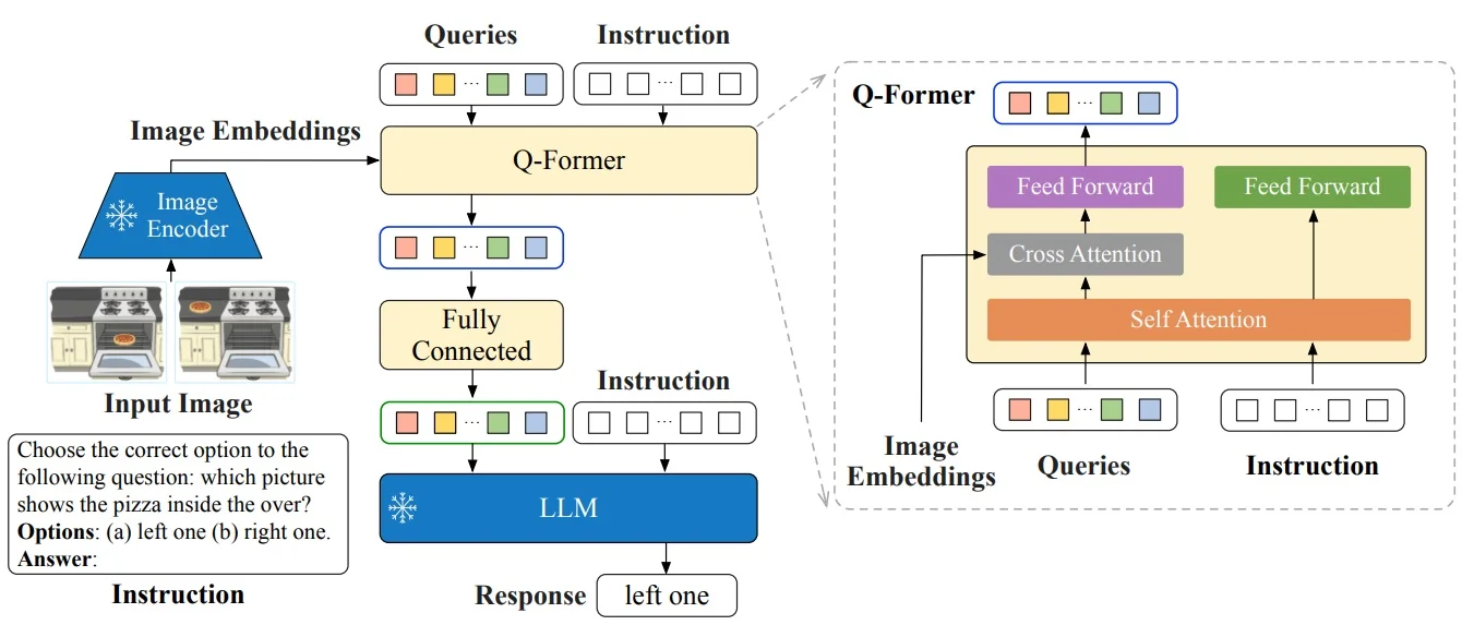
- Instruction-aware Q-Former (task-conditioned queries). Unlike BLIP-2’s task-agnostic queries [343], InstructBLIP [116] fuses the instruction tokens into the Q-Former so that its learnable queries become conditioned on user intent. Concretely, the frozen ViT produces patch features, and the Q-Former receives both these patches and the instruction embeddings. Queries self-attend, then cross-attend to patches while also attending to instructions. This lets them extract instruction-relevant visual evidence (OCR for “read the sign”, spatial reasoning for “which cup is left of the plate?”), instead of a single generic visual summary. This conditioning reduces spurious correlations and disambiguates what to focus on when instructions change at test time.
- Soft visual prompting into a frozen LLM. After \(L_q\) layers, the Q-Former outputs \(K\) query vectors \(Q \in \mathbb {R}^{K \times d}\) which are linearly projected to the LLM’s embedding size, \(\tilde {Q} = QW_p\). These visual prompt tokens are prepended to the instruction tokens and passed to a frozen LLM (e.g., FlanT5, Vicuna). The LLM thus conditions generation on a compact, instruction-aligned “briefing” while preserving its linguistic competence. Compared to BLIP-2, these tokens are instruction-aware and better aligned with the decoding trajectory, improving grounding and factuality.
-
Data flow (end-to-end).
- 1.
- Image \(\rightarrow \) frozen ViT \(\rightarrow \) patch embeddings.
- 2.
- Instruction + learnable queries + patches \(\rightarrow \) Q-Former \(\rightarrow \) instruction-aware queries.
- 3.
- Projection \(W_p\) maps to LLM space, queries prepended to instruction tokens.
- 4.
- Frozen LLM autoregressively generates the response.
- Instruction-tuning objective. For each (instruction, image) \(\mapsto \) response example, the model minimizes next-token LM loss: \[ \mathcal {L}_{\mbox{LM}} = - \sum _m \log p_{\mbox{LLM}}(y_m \mid y_{<m}, \tilde {Q}(\mbox{image}, \mbox{instruction}), \mbox{instruction}), \] updating only the Q-Former and projection layers; both ViT and LLM remain frozen.
Why Instruction Tuning Helps (Intuition) BLIP and BLIP-2 already use LM loss, but their inputs are task-agnostic (generic queries + dataset-formatted prompts). This means the model often learns dataset-specific mappings rather than a general instruction-following procedure. InstructBLIP changes this in two ways:
- 1.
- Instruction-aware Q-Former. Instructions are fused with image tokens, so the Q-Former extracts only the instruction-relevant visual evidence (e.g., text regions for OCR, spatial cues for reasoning) instead of a fixed summary.
- 2.
- Instruction-formatted LM training. Every example is presented as natural instructions with answers, not dataset templates. The LLM is therefore trained to parse arbitrary instructions and ground them in vision.
The difference is subtle but critical: rather than memorizing dataset patterns, the model learns the meta-skill of following instructions—leading to stronger generalization to unseen tasks and more reliable multi-turn interaction.
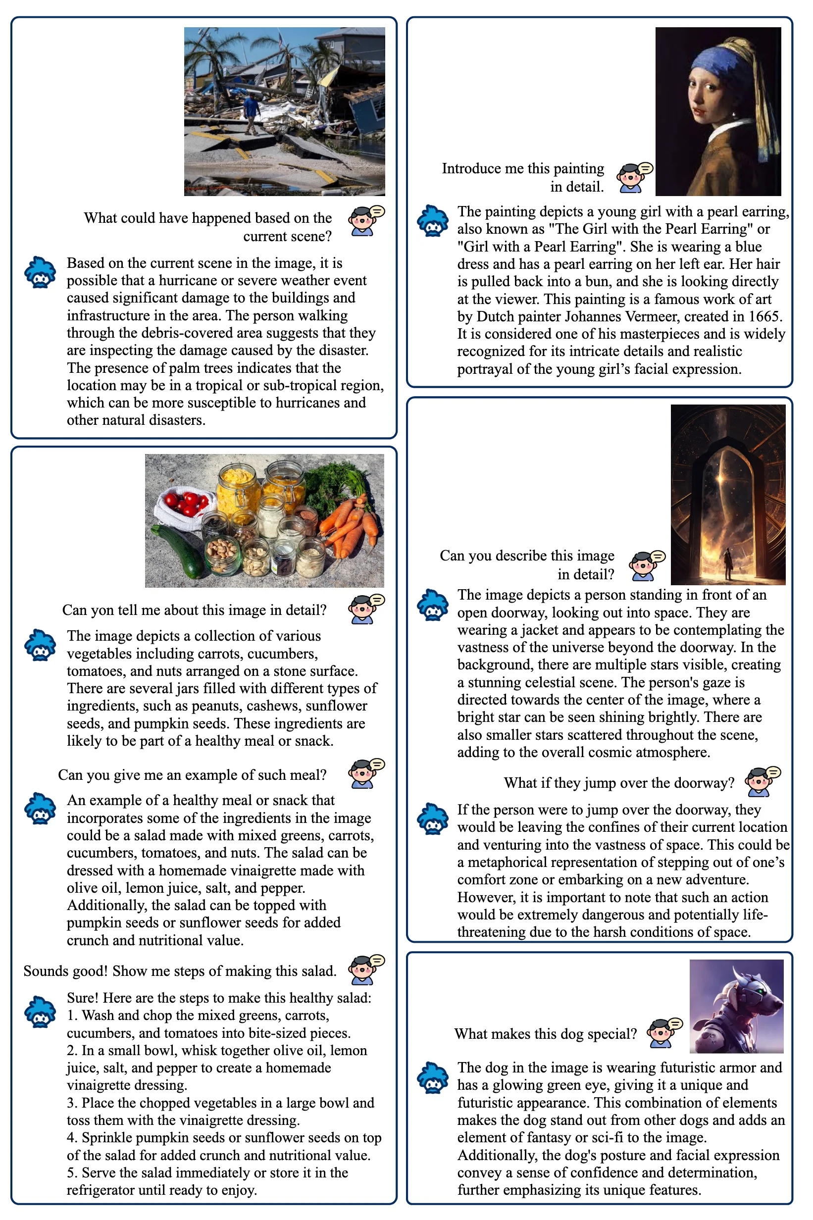
Data & Formatting: From Multi-Task to Instruction-Tuning
- Task coverage. InstructBLIP unifies 26 datasets spanning captioning, VQA (general, OCR, knowledge-grounded), visual reasoning (GQA), visual dialogue (VisDial), video QA (MSVD or MSRVTT), safety (HatefulMemes), and more.
- Prompt templates. Each example is rendered as (Instruction: …, optional Context: …, Image: … \(\rightarrow \) Answer: …). This normalizes heterogeneous supervision into a single instruction-following interface that the LLM already excels at.
- Balanced sampling. A sampling scheme evens exposure across tasks and avoids dominance by large sources (e.g., web captions), improving transfer to held-out tasks and robustness to prompt phrasing.
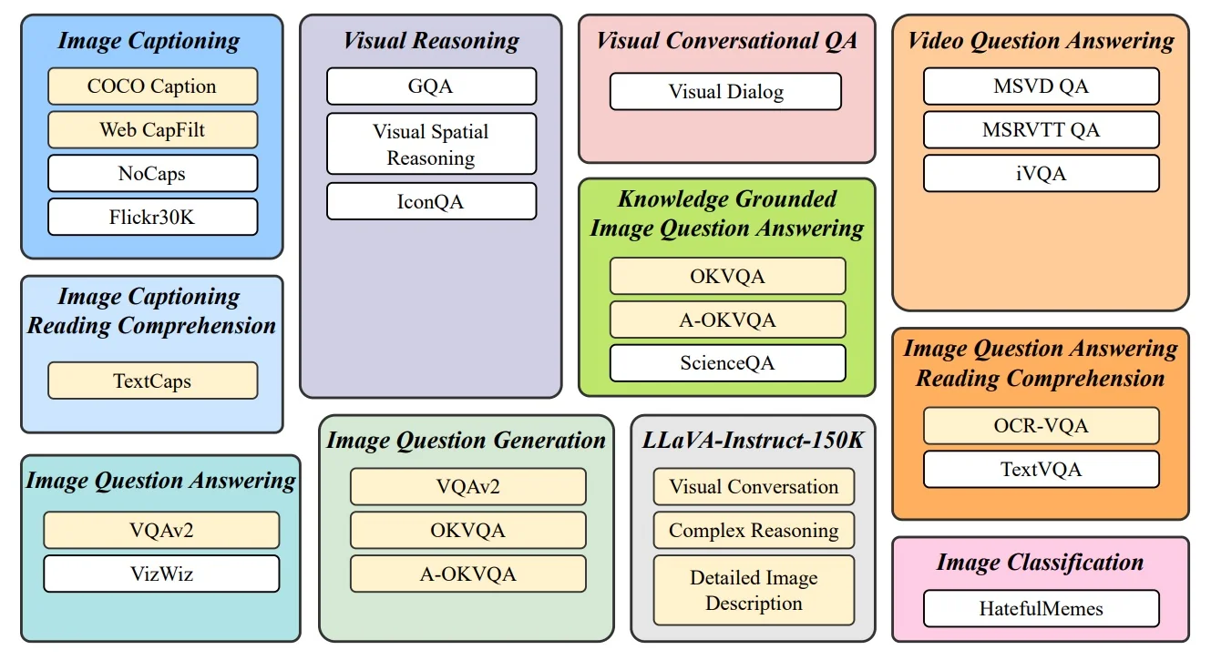
| Method | NoCaps | Flickr30K | GQA | VSR | IconQA | TextVQA | VisDial | HM | VizWiz | SciQA IMG | MSVD QA | MSRVTT QA | iVQA |
|---|---|---|---|---|---|---|---|---|---|---|---|---|---|
| Flamingo-3B [27] | – | 60.6 | – | – | – | 30.1 | – | 53.7 | 28.9 | – | 27.5 | 11.0 | 32.7 |
| Flamingo-9B [27] | – | 61.5 | – | – | – | 31.8 | – | 57.0 | 28.8 | – | 30.2 | 13.7 | 35.2 |
| Flamingo-80B [27] | – | 67.2 | – | – | – | 35.0 | – | 46.4 | 31.6 | – | 35.6 | 17.4 | 40.7 |
| BLIP-2 (FlanT5XL) [24] | 104.5 | 76.1 | 44.0 | 60.5 | 45.5 | 43.1 | 45.7 | 53.0 | 29.8 | 54.9 | 33.7 | 16.2 | 40.4 |
| BLIP-2 (FlanT5XXL) [24] | 98.4 | 73.7 | 44.6 | 68.2 | 45.4 | 44.1 | 46.9 | 52.0 | 29.4 | 64.5 | 34.4 | 17.4 | 45.8 |
| BLIP-2 (Vicuna-7B) | 107.5 | 74.9 | 38.6 | 50.0 | 39.7 | 40.1 | 44.9 | 50.6 | 25.3 | 53.8 | 18.3 | 9.2 | 27.5 |
| BLIP-2 (Vicuna-13B) | 103.9 | 71.6 | 41.0 | 50.9 | 40.6 | 42.5 | 45.1 | 53.7 | 19.6 | 61.0 | 20.3 | 10.3 | 23.5 |
| InstructBLIP (FlanT5XL) | 119.9 | 84.5 | 48.4 | 64.8 | 50.0 | 46.6 | 46.6 | 56.6 | 32.7 | 70.4 | 43.4 | 25.0 | 53.1 |
| InstructBLIP (FlanT5XXL) | 120.0 | 83.5 | 47.9 | 65.6 | 51.2 | 46.6 | 48.5 | 54.1 | 30.9 | 70.6 | 44.3 | 25.6 | 53.8 |
| InstructBLIP (Vicuna-7B) | 123.1 | 82.4 | 49.2 | 54.3 | 43.1 | 50.1 | 45.2 | 59.6 | 34.5 | 60.5 | 41.8 | 22.1 | 52.2 |
| InstructBLIP (Vicuna-13B) | 121.9 | 82.8 | 49.5 | 52.1 | 44.8 | 50.7 | 45.4 | 57.5 | 33.4 | 63.1 | 41.2 | 24.8 | 51.0 |
Ablations: What Matters Two ingredients dominate gains: instruction-aware visual features and balanced sampling. Making the Q-Former conditional on the instruction reliably boosts held-out generalization—especially for knowledge/OCR and instruction-sensitive sets (e.g., large drops on ScienceQA and iVQA when removed). Balanced sampling yields smaller but consistent gains by preventing over-fitting to high-volume tasks; without it, performance regresses across most held-out datasets, with only minor, noisy exceptions.
| Model | Held-in Avg. | GQA | ScienceQA (IMG) | IconQA | VizWiz | iVQA |
|---|---|---|---|---|---|---|
| InstructBLIP (FlanT5XL) | 94.1 | 48.4 | 70.4 | 50.0 | 32.7 | 53.1 |
| w/o Instruction-aware Visual Features | 89.8 | 45.9 ( \(\downarrow \)2.5) | 63.4 ( \(\downarrow \)7.0) | 45.8 ( \(\downarrow \)4.2) | 25.1 ( \(\downarrow \)7.6) | 47.5 ( \(\downarrow \)5.6) |
| w/o Data Balancing | 92.6 | 46.8 ( \(\downarrow \)1.6) | 66.0 ( \(\downarrow \)4.4) | 49.9 ( \(\downarrow \)0.1) | 31.8 ( \(\downarrow \)0.9) | 51.1 ( \(\downarrow \)2.0) |
| InstructBLIP (Vicuna-7B) | 100.8 | 49.2 | 60.5 | 43.1 | 34.5 | 52.2 |
| w/o Instruction-aware Visual Features | 98.9 | 48.2 ( \(\downarrow \)1.0) | 55.2 ( \(\downarrow \)5.3) | 41.2 ( \(\downarrow \)1.9) | 32.4 ( \(\downarrow \)2.1) | 36.8 ( \(\downarrow \)15.4) |
| w/o Data Balancing | 98.8 | 47.8 ( \(\downarrow \)1.4) | 59.4 ( \(\downarrow \)1.1) | 43.5 ( \(\uparrow \)0.4) | 32.3 ( \(\downarrow \)2.2) | 50.3 ( \(\downarrow \)1.9) |
Instruction Tuning vs. Multi-Task Training Plain multi-tasking—either with raw inputs or dataset-tag prompts—learns brittle format\(\to \)answer mappings that score high on held-in sets but fail to transfer. Instruction tuning reframes every example as a natural instruction and routes it through an instruction-aware Q-Former, teaching a general procedure (parse intent \(\rightarrow \) extract relevant evidence \(\rightarrow \) answer). This shift explains the sizeable held-out gains while maintaining competitive held-in scores.
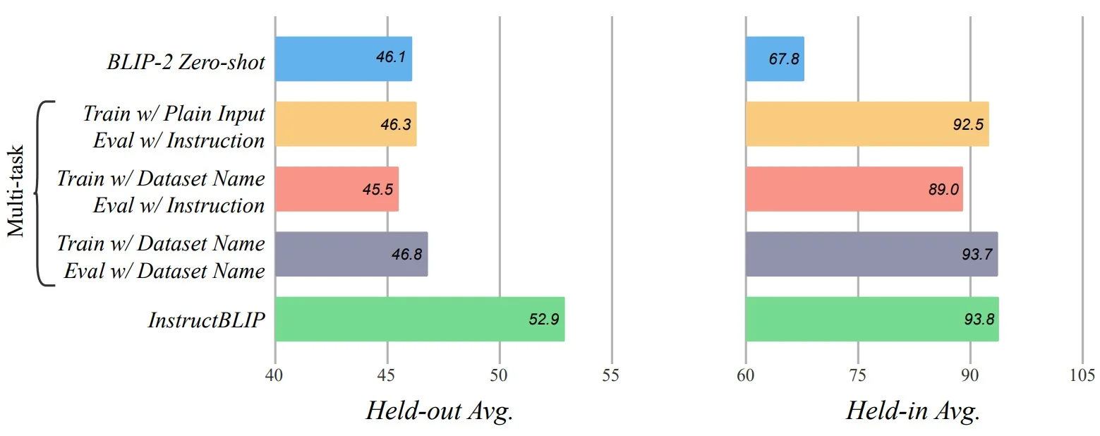
Downstream Fine-Tuning Instruction-tuned checkpoints are superior initializations: they converge faster and reach higher accuracy with modest adaptation, especially on knowledge/OCR-heavy tasks where instruction parsing and targeted visual grounding are pivotal.
| Method | SciQA IMG | OCR-VQA | OKVQA | A-OKVQA Dir Val | A-OKVQA Dir Test | A-OKVQA MC Val | A-OKVQA MC Test |
|---|---|---|---|---|---|---|---|
| Previous SOTA (refs) | [89] 89.0 | [90] 70.3 | [91] 66.1 | [92] 56.3 | [93] 61.6 | [92] 73.2 | [93] 73.6 |
| BLIP-2 (FlanT5XXL) [24] | 89.5 | 72.7 | 54.7 | 57.6 | 53.7 | 80.2 | 76.2 |
| InstructBLIP (FlanT5XXL) [88] | 90.7 | 73.3 | 55.5 | 57.1 | 54.8 | 81.0 | 76.7 |
| BLIP-2 (Vicuna-7B) [24] | 77.3 | 69.1 | 59.3 | 60.0 | 58.7 | 72.1 | 69.0 |
| InstructBLIP (Vicuna-7B) [88] | 79.5 | 72.8 | 62.1 | 64.0 | 62.1 | 75.7 | 73.4 |
Takeaways (Sharper Reading of the Evidence) Instruction-conditioning is the main driver of transfer: removing it collapses iVQA (Vicuna, \(-15.4\)) and significantly hurts ScienceQA (up to \(-7.0\)), signalling that which visual evidence to extract depends on the instruction. Balanced sampling stabilizes cross-task learning, trimming smaller but pervasive regressions when ablated. Together, these choices explain why instruction-tuned checkpoints fine-tune better than BLIP-2 baselines across diverse downstream tasks.
Limitations and Future Work A central limitation of InstructBLIP [116] is that it is fundamentally image-centric. Its Q-Former provides only a narrow “visual prompt” interface to the LLM, and although effective for single-image instruction following, it cannot natively capture motion, temporal order, or long-horizon dynamics. Early attempts to handle video defaulted to uniform frame sampling and concatenation of features, which ignores motion cues and collapses temporal structure.
Historical trajectory.
- BLIP and BLIP-2 (2022–2023). Built for image–text pretraining and instruction tuning, these models demonstrated strong zero-shot transfer but lacked any temporal component. Video QA benchmarks (e.g., MSRVTT-QA) were approached by concatenating features from 4–16 uniformly sampled frames, producing workable results but with no explicit modeling of sequence order or causality.
- Immediate adaptations. Several derivatives (Video-BLIP, X-InstructBLIP, Video-LLaMA, MiniGPT4-Video) extended the image-focused architecture to video by adding lightweight temporal pooling, video-specific Q-Formers, or scaling up to dozens of sampled frames. These efforts confirmed the flexibility of BLIP-2/LLaVA-style stacks, yet they remained stopgaps: temporal reasoning was approximated rather than integrated, and training objectives were still defined at the frame or image level.
Broader limitations. Beyond video, InstructBLIP also inherits dataset and prompt biases, struggles with fine-grained grounding, and lacks support for multi-step tool use or retrieval. Its reliance on a frozen LLM limits adaptability to new domains or safety-critical reasoning.
The LLaVA line of work.
- LLaVA (2023). Bridged frozen CLIP-style encoders with an LLM to enable multimodal dialogue on images. Video extensions (“Video-LLaVA”) treated clips as sets of frames, essentially multi-image interleaving, which worked in practice but without native temporal encoding.
- LLaVA-NeXT (2024). Addressed another bottleneck—resolution. With its AnyRes tiling and merging strategy, higher-resolution visual tokens could be processed without aggressive downsampling, and interleaved multi-image support was improved. Yet video remained a weak spot: sequences were still modeled as unordered image sets with no explicit temporal attention or objectives.
- LLaVA-OneVision (2024). Represented a turning point. It unified support for images, image sets, and multi-frame clips through a single tokenization path, introduced time-aware positional embeddings and attention across frames, and trained on mixed video and image data. This enabled native video QA and stronger cross-domain transfer, though challenges remained around long-horizon clips and efficient handling of motion-rich inputs.
Future directions (as implied by these limits). The trajectory from BLIP to LLaVA-OneVision highlights both progress and remaining gaps. Key next steps include:
- Temporal modeling as a core design. Moving beyond frame concatenation toward temporal Q-Formers, causal attention, and efficient video transformers to natively capture motion and sequence structure.
- Scaling instruction coverage. Broadening instruction tuning across languages, domains, and safety-critical contexts to ensure generalization beyond static-image corpora.
- Retrieval and tool grounding with time. Extending retrieval-augmented generation and tool use to temporal settings, linking entities and events across frames or moments in a clip.
In short, the field evolved from static image instruction tuning (BLIP/InstructBLIP) \(\rightarrow \) pragmatic video extensions (Video-LLaVA, MiniGPT4-Video, X-InstructBLIP) \(\rightarrow \) stronger but still image-biased upgrades (LLaVA-NeXT) \(\rightarrow \) first-class multimodal unification in LLaVA-OneVision [377, 339, 335]. The logical next step is to make temporal reasoning and retrieval-native grounding as central as resolution and instruction-following have become, starting with LLaVA [377]
Enrichment 24.7.2: LLaVA: Large Language and Vision Assistant
High-Level Idea LLaVA [377] couples a strong frozen vision encoder (CLIP ViT-L/14) with an instruction-tuned LLM (Vicuna) via a lightweight linear projector. Rather than learning a query bridge (e.g., BLIP-2’s Q-Former), LLaVA emphasizes instruction-following by training on GPT-4–curated visual instruction data (constructed from captions/boxes but generated without showing images to GPT-4).
Architecture Given image \(X_v\), a frozen CLIP encoder produces grid features \(Z_v=g(X_v)\). A trainable linear map \(W\) projects \(Z_v\) into the LLM embedding space to form visual tokens \(H_v=WZ_v\), which are prepended/interleaved with text tokens. The model fine-tunes the LLM (often with PEFT/LoRA) using the standard autoregressive LM loss on assistant tokens; the CLIP encoder remains frozen and no cross-attention/Q-Former is used: \[ H_v = W \cdot Z_v,\qquad Z_v = g(X_v). \]
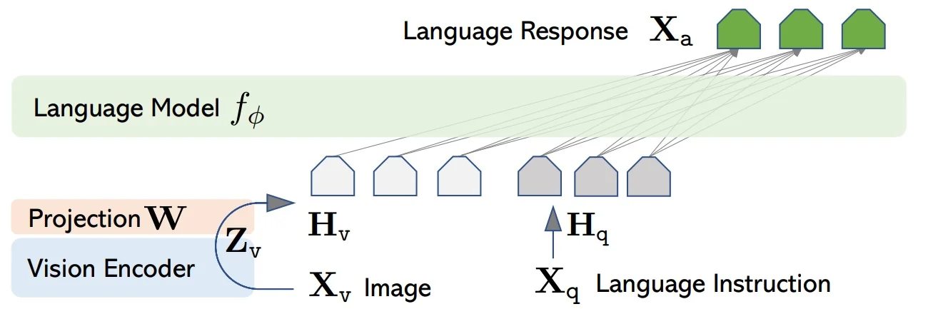
Why freeze vision but (partly) train the LLM?
- Protect a strong visual prior. CLIP ViT-L/14 is already trained on massive image–text corpora; the LLaVA instruction set is comparatively small. Freezing CLIP avoids catastrophic forgetting and preserves broad zero-shot visual semantics.
- Put learning where the skill lives. Instruction following is largely a language-side procedure (parse intent, plan, verbalize). Fine-tuning the LLM (typically with PEFT/LoRA in practice) teaches it to use visual tokens as part of that procedure; the connector \(W\) just makes CLIP features legible to the LLM.
-
Alignment, not re-seeing. The main gap is modal alignment: map \(Z_v=g(X_v)\) into the LLM’s token space and adapt the LLM to condition on those tokens. Training a tiny projector \(W\) plus (adapter) updates in the LLM empirically suffices; re-training vision isn’t necessary for instruction-following chat.
- Compute reality (clarified). Full LLM fine-tuning is expensive in absolute FLOPs, and the LLM is much larger than CLIP. LLaVA mitigates this by (i) freezing the vision tower entirely, (ii) keeping the connector minimal (linear/MLP), and (iii) often using PEFT on the LLM. This keeps memory stable and concentrates updates where they matter most for following instructions.
-
Two-stage recipe.
- 1.
- Projector warmup. First, only the lightweight projection layer \(W\) is trained on standard image–text pairs, while both the CLIP encoder and the LLM remain frozen. This aligns CLIP’s visual features with the LLM’s embedding space so that visual tokens are “readable” by the language model.
- 2.
- Visual instruction tuning. In this stage, \(W\) and the LLM are fine-tuned together on multimodal instruction–response pairs that were automatically generated with GPT-4. Since high-quality human-labeled instruction data for images is scarce, GPT-4 is prompted with captions or region annotations to synthesize diverse, instruction-style questions and detailed answers. This produces a large, consistent, and coherent instruction set, allowing the LLM to learn how to weave the projected visual tokens into its reasoning and response generation. The CLIP encoder remains frozen throughout.
Contrast to BLIP-2. BLIP-2 freezes both experts and learns a Q-Former (cross-attention queries) as a task-aware bridge; the LLM is kept frozen during pretraining. LLaVA instead uses a simple projector and invests supervision on the LLM side (instruction-tuning), yielding strong conversational adherence with low fusion complexity—at the cost of less structured, query-driven grounding than a learned cross-attention module.
Data Pipeline: Visual Instruction Tuning A central innovation in LLaVA [377] is how its training data is generated. Importantly, GPT–4 never sees the raw images themselves. Instead, each image is first turned into textual proxies—such as captions or detected object labels with bounding boxes—which are then fed to GPT–4. Using this context, GPT–4 is asked to write instruction \(\rightarrow \) response examples that look like real multimodal conversations.
-
Input contexts. For every image, the system prepares:
- Captions: several diverse captions describing different aspects of the scene.
- Box labels: object categories together with their bounding box coordinates, giving GPT–4 a more structured picture of what is present and where.
-
Three kinds of responses. GPT–4 is asked to produce answers in three styles:
- 1.
- Conversational Q&A: short multi-turn dialogues (teaches the model to follow chat-style prompts).
- 2.
- Detailed descriptions: long-form outputs covering fine details (trains thorough grounding and coverage).
- 3.
- Complex reasoning: explanations that require commonsense or multi-step inference (pushes the model beyond surface description).
These three types were chosen to cover complementary skills: dialogue flow, exhaustive detail, and reasoning. Ablations in the paper confirm that using all three leads to the strongest results.
- Why this setup? At the time, no large public dataset of multimodal instructions existed. By repurposing image captions and object detections into prompts, and letting GPT–4 spin them into diverse instruction–response pairs, the authors created a scalable, stylistically consistent training set. This gave the LLM practice in “talking about images” without needing humans to hand-label every dialogue.
- Training format. The generated dialogues are wrapped in Vicuna’s chat template (system \(\rightarrow \) user \(\rightarrow \) assistant). During training, only the assistant tokens are used for the autoregressive loss, teaching the LLM to generate natural, instruction-following replies conditioned on the projected visual tokens.
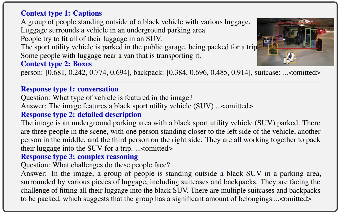
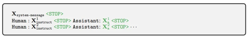
Why It Works (vs. BLIP/BLIP-2)
-
Connector simplicity. LLaVA uses only a lightweight linear projector to map CLIP features into the LLM’s embedding space. This avoids the complexity of Q-Former cross-attention or gated modules, making training straightforward and connector overhead negligible.
- Instruction-first supervision. Instead of contrastive alignment or captioning, LLaVA trains directly on GPT-4–curated multimodal instructions. This supervision style teaches the LLM to follow instructions about images (e.g., “what is unusual?”) rather than merely align embeddings. BLIP and BLIP-2 never explicitly target this behavior in pretraining.
- Trade-offs vs. BLIP-2. BLIP-2 keeps both CLIP and the LLM frozen and learns a small Q-Former bridge—highly compute-efficient and stable, with strong zero-shot priors. LLaVA instead fine-tunes the LLM (together with the projector), investing in instruction-following fluency. The benefit is stronger conversational ability and instruction adherence; the drawback is weaker structured grounding and greater dependence on the synthetic instruction data distribution.
- Inference cost. Unlike BLIP-2’s compact query tokens, LLaVA passes a large number of projected CLIP grid features (hundreds of tokens at 336px input) into the LLM. This increases sequence length and thus slows inference, while also raising memory use. In practice, LLaVA trades some efficiency for richer supervision and stronger dialogue fluency.
Instruction Following and Reasoning (Qualitative)
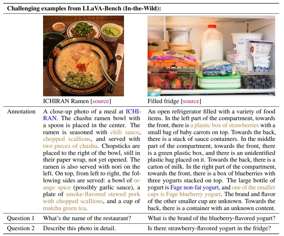
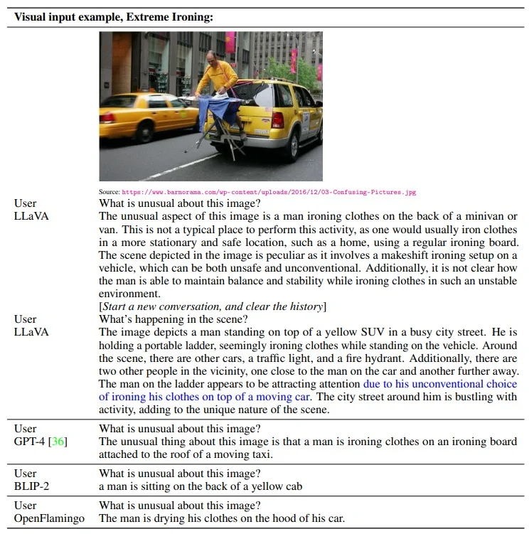
Benchmarks: LLaVA-Bench, COCO ablations, In-the-Wild, ScienceQA
| Training data | Conversation | Detail desc. | Complex reasoning | All |
|---|---|---|---|---|
| Full data | 83.1 | 75.3 | 96.5 | 85.1 |
| Detail + Complex | 81.5 ( \(\downarrow \)1.6) | 73.3 ( \(\downarrow \)2.0) | 90.8 ( \(\downarrow \)5.7) | 81.9 ( \(\downarrow \)3.2) |
| Conv + 5% Detail + 10% Complex | 81.0 ( \(\downarrow \)2.1) | 68.4 ( \(\downarrow \)7.1) | 91.5 ( \(\downarrow \)5.0) | 80.5 ( \(\downarrow \)4.4) |
| Conversation | 76.5 ( \(\downarrow \)6.6) | 59.8 ( \(\downarrow \)16.2) | 84.9 ( \(\downarrow \)12.4) | 73.8 ( \(\downarrow \)11.3) |
| No Instruction Tuning | 22.0 ( \(\downarrow \)61.1) | 24.0 ( \(\downarrow \)51.3) | 18.5 ( \(\downarrow \)78.0) | 21.5 ( \(\downarrow \)63.6) |
| Method | Conversation | Detail desc. | Complex reasoning | All |
|---|---|---|---|---|
| OpenFlamingo [96] | \(19.3 \pm 0.5\) | \(19.0 \pm 0.5\) | \(19.1 \pm 0.7\) | \(19.1 \pm 0.4\) |
| BLIP-2 [24] | \(54.6 \pm 1.4\) | \(29.1 \pm 1.2\) | \(32.9 \pm 0.7\) | \(38.1 \pm 1.0\) |
| LLaVA [89] | \(57.3 \pm 1.9\) | \(52.5 \pm 6.3\) | \(81.7 \pm 1.8\) | \(67.3 \pm 2.0\) |
| LLaVA\(^\dagger \) [89] | \(58.8 \pm 0.6\) | \(49.2 \pm 0.8\) | \(81.4 \pm 0.3\) | \(66.7 \pm 0.3\) |
| Method | NAT | SOC | LAN | TXT | IMG | NO | G1-6 | G7-12 | Average |
|---|---|---|---|---|---|---|---|---|---|
Representative & SoTA numbers reported in literature |
|||||||||
| Human [97] | 90.23 | 84.97 | 87.48 | 89.60 | 87.50 | 88.10 | 91.59 | 82.42 | 88.40 |
| GPT-3.5 [97] | 74.64 | 69.74 | 76.00 | 74.44 | 67.28 | 77.42 | 76.80 | 68.89 | 73.97 |
| GPT-3.5 w/ CoT [97] | 75.44 | 70.87 | 78.09 | 74.68 | 67.43 | 79.93 | 78.23 | 69.68 | 75.17 |
| LLaMA-Adapter [98] | 84.37 | 88.30 | 84.36 | 83.72 | 80.32 | 86.90 | 85.83 | 84.05 | 85.19 |
| MM-CoTBase [99] | 87.52 | 77.17 | 85.82 | 87.88 | 82.90 | 86.83 | 84.65 | 85.37 | 84.91 |
| MM-CoTLarge [99] | 95.91 | 82.00 | 90.82 | 95.26 | 88.80 | 92.89 | 92.44 | 90.31 | 91.68 |
Author runs |
|||||||||
| GPT-4\(^\dagger \) | 84.06 | 73.45 | 87.36 | 81.87 | 70.75 | 90.73 | 84.69 | 79.10 | 82.69 |
| LLaVA [89] | 90.36 | 95.95 | 88.00 | 89.49 | 88.00 | 90.66 | 90.93 | 90.90 | 90.92 |
| LLaVA+GPT-4\(^\dagger \) (complement) | 90.36 | 95.50 | 88.55 | 89.05 | 87.80 | 91.08 | 92.22 | 88.73 | 90.97 |
| LLaVA+GPT-4\(^\dagger \) (judge) | 91.56 | 96.74 | 91.09 | 90.62 | 88.99 | 93.52 | 92.73 | 92.16 | 92.53 |
| Visual features | Before | Last |
|---|---|---|
| Best variant | 90.92 | 89.96 ( \(\downarrow \)0.96) |
| Predict answer first | – | 89.77 ( \(\downarrow \)1.15) |
| Training from scratch | 85.81 ( \(\downarrow \)5.11) | – |
| 7B model size | 89.84 ( \(\downarrow \)1.08) | – |
What the Ablations Say (and How This Differs from BLIP-2)
- Instruction tuning is essential. Removing it collapses performance (Table 24.42), confirming that formatting everything as natural-language instructions teaches a reusable procedure for solving diverse tasks—similar insight to InstructBLIP, but achieved with a simpler connector.
-
Visual feature choice matters. Using the right CLIP layer (pre-/post-last) impacts downstream QA (Table 24.45); BLIP-2 instead learns a task-aware query interface (Q-Former), while LLaVA must pick a fixed feature tap.
- Training dynamics. Starting “from scratch” (no Vicuna init) underperforms strongly, emphasizing the value of strong LLM priors—the same high-level lesson as BLIP-2, but LLaVA fine-tunes the LLM, whereas BLIP-2 keeps it frozen and tunes only a small bridge.
- Connector vs. Instruction Data. BLIP-2 invests in a learned bridge (Q-Former) to translate vision for a frozen LLM; LLaVA keeps the bridge simple (linear) and invests in instruction data + LLM fine-tuning.
- Efficiency. BLIP-2 trains far fewer parameters (frozen experts), typically more stable and compute-efficient. LLaVA trains more on the language side (often with PEFT/LoRA), improving conversationality and adherence to instructions at the cost of more sensitivity to data curation.
- Generalization. BLIP-2’s priors excel in zero-shot retrieval/grounding with robust visual features; LLaVA often wins on instruction-following and free-form dialogue (LLaVA-Bench), but is more dependent on the prompt style and instruction distribution.
Limitations and Next Steps (segue to LLaVA-NeXT / OneVision) While LLaVA [377] proved that a frozen CLIP encoder plus an instruction-tuned LLM can deliver strong multimodal dialogue, it remains fundamentally image-centric. Videos are only approximated by feeding multiple frames as separate images, which ignores motion and temporal dependencies. High-resolution images are globally resized, often losing small details, and the linear projector provides only a minimal bridge for multi-image reasoning.
LLaVA-NeXT [339] was introduced to address some of these gaps. It brought two notable upgrades:
- AnyRes. A tiling-and-merging strategy that allows images to be processed at near-native resolution without heavy downsampling, crucial for fine-grained perception such as OCR or small-object recognition.
- Multi-image interleaving. A mechanism to encode several images jointly within a conversation, enabling set-level reasoning across multiple inputs.
Together, these improvements boosted LLaVA’s ability to handle high-resolution and multi-image tasks. However, NeXT still lacks native temporal modeling: video frames are treated as a loose set of images with no explicit time encoding, motion cues, or sequence objectives.
This motivates the next step: LLaVA-OneVision [335]. Instead of treating video as “many images,” it trains on a mixture of video and image data, introduces time-aware positional tokens and attention mechanisms, and strengthens visual token pooling to fit longer sequences within the LLM’s context budget. The result is a model that can natively support video question answering while retaining the instruction-following strengths of its predecessors.
In short, NeXT overcame resolution and multi-image limits of LLaVA, but it is OneVision that finally closes the modality gap—moving from image-centric adaptation to unified handling of single images, multi-image sets, and full video clips.
Enrichment 24.7.3: LLaVA-OneVision: Unified Multimodal Transfer
From LLaVA to OneVision: Motivation & Goal LLaVA showed that a minimal pipeline—frozen vision encoder \(\rightarrow \) lightweight projector \(\rightarrow \) instruction-tuned LLM—can produce a strong image-centric assistant. Yet three gaps remained: (i) set-level reasoning across multiple images lacked structure, (ii) video was only approximated by feeding frames as independent stills (no temporal modeling), and (iii) aggressive global resizing hurt high-resolution perception (OCR, diagrams, small objects). LLaVA-OneVision [335] addresses these gaps with a single, unified model that natively supports single-image, multi-image, and video inputs and encourages cross-scenario skill transfer, while preserving LLaVA’s minimalist spirit.
High-Level Idea OneVision keeps the simple connector-to-LLM philosophy but upgrades the visual pipeline and tokenization so that (a) high-resolution details are preserved, (b) token budgets remain balanced across modalities, and (c) temporal order/motion are modeled directly. A staged curriculum first aligns vision tokens to the LLM, then builds a strong single-image instruction follower, and finally mixes in multi-image & video data to induce native temporal reasoning and cross-scenario transfer.
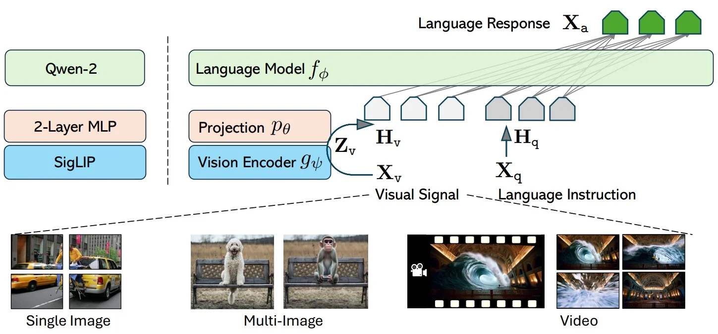
Method
Architecture Overview (What changes vs. LLaVA)
-
Vision encoder & projector (minimal fusion, stronger backbone). As in LLaVA, visual inputs are encoded by a pretrained vision tower and mapped into the LLM token space by a small projector (2-layer MLP / linear). OneVision upgrades the tower from CLIP to the SigLIP family (typical input \(384{\times }384\)), chosen for its robust open-source zero-shot alignment and strong text-rich perception. The projector remains the only bespoke fusion block, so visual tokens can be simply prepended/interleaved with text—preserving LLaVA’s low-complexity path (no cross-attention/Q-Former).
-
Higher-resolution processing (Higher AnyRes). OneVision replaces global resizing with an adaptive tile \(\rightarrow \) encode \(\rightarrow \) merge pipeline that preserves local detail and keeps the visual sequence length predictable [335].
- 1.
- Tiling (detail + context). From a high-resolution image, build two kinds of inputs: (i) a global view obtained by uniformly resizing the full image to the vision encoder’s native resolution (e.g., \(384{\times }384\)), and (ii) an \(a{\times }b\) grid of aspect-preserving local crops, each also resized to the encoder’s native resolution. The global view provides coarse layout; the tiles preserve fine text/edges that a single global downscale would destroy.
- 2.
- Encoding (shared backbone). Feed the global view and each of the \(a{\times }b\) crops independently through the frozen vision encoder (e.g., SigLIP), producing \(T\) tokens per input (e.g., \(T{=}729\) for a \(384{\times }384\) input). The provisional visual-token length is \[ L \;=\; (a\times b + 1)\,T, \] where the “\(+1\)” accounts for the global view.
- 3.
- Budgeting & concatenation (Higher AnyRes). To keep sequence length predictable, impose a per-scenario token cap \(\tau \). If \(L\!>\!\tau \), reduce the tokens per input (global and each crop) by bilinearly interpolating their feature grids before flattening: \[ T_{\mbox{new}} \;=\; \Big \lfloor \tfrac {\tau }{a\times b + 1} \Big \rfloor , \quad \mbox{so that}\quad L_{\mbox{new}} \;=\; (a\times b + 1)\,T_{\mbox{new}} \le \tau . \] Finally, concatenate the token sequences from the global view and all crops in a fixed order to form the visual-token stream for the projector/LLM. No cross-scale feature blending is introduced; the “merge” is achieved by length-controlled per-input downsampling plus sequence concatenation. This preserves local detail (via tiles) and global context (via the base image) while preventing quadratic attention blow-up and keeping tokens consistent across inputs of widely varying native resolution [335].
Why this works. The global view provides a coarse anchor of scene layout and long-range object relations, while the local crops contribute high-frequency detail such as OCR strokes or small parts. Rather than fusing feature maps, the method simply concatenates tokens from both sources, ensuring that context and detail coexist in the same token stream. When the provisional length exceeds a per-scenario cap, bilinear interpolation is applied at the feature-grid level to shrink tokens per input uniformly, preserving continuity while enforcing the budget. This guarantees that the LLM always receives consistent, high-fidelity tokens across images of widely varying native resolutions, without quadratic blow-up or architectural changes. In practice, this directly addresses LLaVA’s high-resolution failure modes (e.g., documents, charts, dense UI screens) while keeping the downstream language model untouched [335].
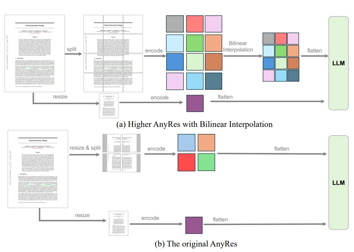
Figure 24.63: Higher AnyRes vs. original AnyRes. Upgraded tiling/merging with bilinear interpolation preserves high-resolution fidelity (top) compared to the original scheme (bottom), improving OCR and small-object recognition. Source: [335]. -
Balanced visual token budgets (cross-scenario parity). To promote skill transfer while respecting the LLM’s context, OneVision normalizes the number of visual tokens per scenario to be of the same order, using a common “unit”: the token count from one SigLIP view at \(384{\times }384\) (about \(T{=}729\) tokens) [335]. Let an image be tiled into an \(a{\times }b\) grid (with an additional resized global view, “\(+1\)”). The provisional length is \[ L \;=\; (a{\times }b + 1)\, T. \]
A per-scenario threshold \(\tau _s\) (with \(s\!\in \!\{\mbox{single-image (SI)},\ \mbox{multi-image (MI)},\ \mbox{video (VID)}\}\)) is enforced before concatenating visual tokens with text. The goal is to keep SI, MI, and VID inputs in the same token range so no modality dominates the context [335]. For a tiled single image with grid \(a{\times }b\) plus one global view, the provisional length is \[ L_{\mbox{SI}} \;=\; (a{\times }b + 1)\,T. \] For \(m\) independent images in MI (each near the base unit), \(L_{\mbox{MI}} \!\approx \! m\,T\). For a video with \(f\) frames, \(L_{\mbox{VID}} \!\approx \! f\,T_{\mbox{frame}}\) (with \(T_{\mbox{frame}}\) obtained via feature-space interpolation per frame). If \(L_s \!>\! \tau _s\), the loader applies uniform feature-grid downsampling so that each view contributes \[ T_{\mbox{new}} \;=\; \Big \lfloor \frac {\tau _s}{N_s} \Big \rfloor \quad \mbox{with}\quad N_s \;=\; \begin {cases} a{\times }b+1 & (s=\mbox{SI})\\ m & (s=\mbox{MI})\\ f & (s=\mbox{VID}) \end {cases} \] and thus \(N_s\,T_{\mbox{new}} \le \tau _s\). Downsampling is implemented by bilinear pooling on the encoder feature maps (token grids), preserving spatial continuity while meeting the budget [335]. Concretely:
- Single image (SI / High AnyRes). Choose a small tile grid (e.g., global \(+\) up to \(3{\times }3\) crops). If \((a{\times }b{+}1)T \!>\! \tau _{\mbox{SI}}\), either reduce the grid (e.g., \(3{\times }3\!\to \!2{\times }2\)) or apply bilinear pooling so that each view contributes \(\lfloor \tau _{\mbox{SI}}/(a{\times }b{+}1)\rfloor \) tokens [335].
- Multi-image (MI). Admit up to \(m{\le }12\) images. If \(mT \!>\! \tau _{\mbox{MI}}\), uniformly shrink per-image token grids to \(T_{\mbox{new}}\!=\!\lfloor \tau _{\mbox{MI}}/m\rfloor \), keeping the total comparable to a high-res single image [335].
- Video (VID). Sample up to \(f{\le }32\) frames. Per-frame features are pooled (e.g., \(2{\times }2\) bilinear) to \(\approx \!196\) tokens/frame; if \(f\cdot 196 \!>\! \tau _{\mbox{VID}}\), reduce \(f\) (FPS-aware sub-sampling) and/or increase pooling so \(T_{\mbox{frame,new}}\!=\!\lfloor \tau _{\mbox{VID}}/f\rfloor \) [335].
Why this helps. Setting \(\tau _{\mbox{SI}},\tau _{\mbox{MI}},\tau _{\mbox{VID}}\) to similar magnitudes yields cross-scenario parity: tiled single images, multi-image sets, and short clips contribute comparable visual budgets. This prevents context monopolization, stabilizes SFT across modalities, and—crucially—makes a tiled image appear budget-wise like a short sequence, encouraging routines (scan, compare, summarize) that transfer between SI, MI, and VID without changing the downstream language model [335].
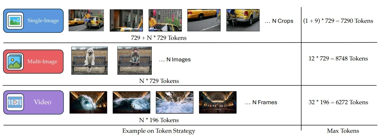
Figure 24.64: Balanced visual token allocation across modalities. OneVision caps tokens so single-image, multi-image, and video inputs receive comparable visual capacity (e.g., \(\sim \)729 tokens \(\approx \) SigLIP at \(384{\times }384\)), preserving LLM context and encouraging cross-scenario transfer. Source: [335]. -
Temporal indexing & attention (native video modeling). Videos are represented as an ordered sequence of frame tokens and rely on the LLM’s inherent sequence modeling for temporal understanding—no bespoke video module is introduced [335]. Concretely:
- 1.
- Frame sampling & features. Sample up to 32 frames (FPS-aware for long clips). Each frame is resized to the encoder’s native resolution (e.g., \(384{\times }384\)), encoded by the frozen vision tower, then downsampled in feature space using \(2{\times }2\) bilinear interpolation to a per-frame budget of \(\approx 196\) tokens (Appendix C.1; Fig. “Higher AnyRes”) [335].
- 2.
- Implicit time via order (no extra temporal PE required). The 2D spatial positional encodings from the vision encoder are retained; frames are concatenated in chronological order into one stream, prefixed by a single <image> marker for the entire video (Appendix C.2) [335]. The paper does not introduce a separate learned or sinusoidal temporal embedding; the position in the sequence itself encodes time.
- 3.
- Causal attention over the sequence. The resulting token stream is fed to the LLM with standard causal/self-attention (lower-triangular masking), which preserves temporal direction. This enables queries such as “what happens next,” change detection, and event localization while keeping LLaVA’s minimalist fusion design intact [335].
Why it works. Chronological concatenation makes inter-frame differences addressable through relative positions in the same attention space as language; causal flow lets the LLM compose motion narratives (e.g., “the door opens after the person reaches the handle”). Combined with the per-frame token budget (\(\sim \)196) and the cap on total frames (32), this provides stable compute and strong zero-/few-shot video QA via transfer from image training [335].
Training Curriculum (How capabilities are built) The recipe follows a progressive curriculum that first forges a clean interface between vision and language, then injects knowledge at higher visual fidelity, and finally teaches instruction-following across scenarios. Each stage increases difficulty in one axis at a time (trainable scope, resolution/token budget, task diversity), which stabilizes optimization and preserves pretrained priors [335].
- 1.
- Stage 1: Language–Image Alignment (frozen experts). What we do. Freeze the vision encoder and the LLM; train only the lightweight projector on \({\sim }558\mbox{K}\) image–text pairs at the encoder’s native resolution (e.g., \(384{\times }384\) \(\Rightarrow \) \(\approx 729\) tokens per view). Intuition. Treat the projector like a translator that learns the “alphabet” of visual features so the LLM can read them, without editing either expert’s hard-earned priors. Why first. Updating only a tiny module gives fast, stable alignment and avoids catastrophic forgetting; it also removes noisy gradients before scaling resolution or adding complex instructions. What emerges. Zero-shot basics (captioning, simple QA) with a clean, low-variance interface the later stages can safely build on [335].
- 2.
- Stage 1.5: High-Quality Knowledge Learning (full model, Higher AnyRes). What we do. Unfreeze the full stack (vision encoder, projector, LLM) and continue training on \({\sim }4\mbox{M}\) high-quality single-image samples. In the meanwhile, it is done while enabling Higher AnyRes (tile\(\rightarrow \)encode\(\rightarrow \)merge). Token budgets are increased progressively (e.g., up to \(\sim 5{\times }\) the base) so the model learns to cope with more detail without instability. Intuition. After the “alphabet”, this is reading widely: infuse broad perceptual/world knowledge and teach the model to process dense inputs (documents, charts, UI screens) at near-native resolution. Why now. Once the interface is stable, end-to-end updates can safely propagate knowledge into both experts while AnyRes habituates the model to larger, but controlled, visual sequences. What emerges. Better grounding for fine text and small parts, plus robustness to resolution changes—fixing the original LLaVA’s global-resize bottleneck [335].
- 3.
- Stage 2: Visual Instruction Tuning (full model). Goal. Teach
the model to follow instructions across scenarios while keeping visual
tokens within balanced budgets.
- 2a: Single-Image SFT (3.2M). What we do. Supervised instruction tuning on a curated single-image corpus covering general QA/captioning, docs/charts/screens (OCR-heavy), visual math/reasoning, and multilingual prompts. AnyRes is used when detail matters; token caps preserve room for the prompt and answers. Intuition. Like practicing conversations before debates: establish reliable, step-by-step response behavior on the scenario with the richest data (images) and the widest skill coverage. What emerges. A strong, dependable image assistant—good habits in formatting, chain-of-thought style reasoning (when supervised), and grounding to visual evidence [335].
- 2b: OneVision SFT (1.6M mixed). What we do. Instruction tune on a balanced mixture of multi-image + video + single-image samples using the same connector and tokenization path. Multi-image sets and video clips are normalized to comparable visual-token budgets (e.g., up to \(12\) images near the base unit; up to \(32\) frames at \(\sim 196\) tokens/frame via \(2{\times }2\) feature-space interpolation). Frames are ordered chronologically; the sequence is fed directly to the LLM [335]. Intuition. This is cross-training: by keeping budgets comparable, a tiled high-res image “looks like” a short sequence, and a frame sequence “looks like” an interleaved set—so the LLM reuses the same routines (scan, compare, summarize, localize changes). Why mixed (not siloed). Mixing prevents modality-specific overfitting and encourages transfer: OCR skill from images helps in videos; “spot-the-difference” across images helps temporal change detection. What emerges. Native support for multi-image reasoning and temporal understanding (event order, causal queries) without bespoke video modules, while retaining single-image strengths [335].
Takeaway. The staged path—align \(\rightarrow \) enrich at higher resolution \(\rightarrow \) generalize via balanced, mixed instructions—keeps training stable, preserves priors, and yields a single open model that natively handles single-image, multi-image, and video inputs using the same minimalist connector [335].
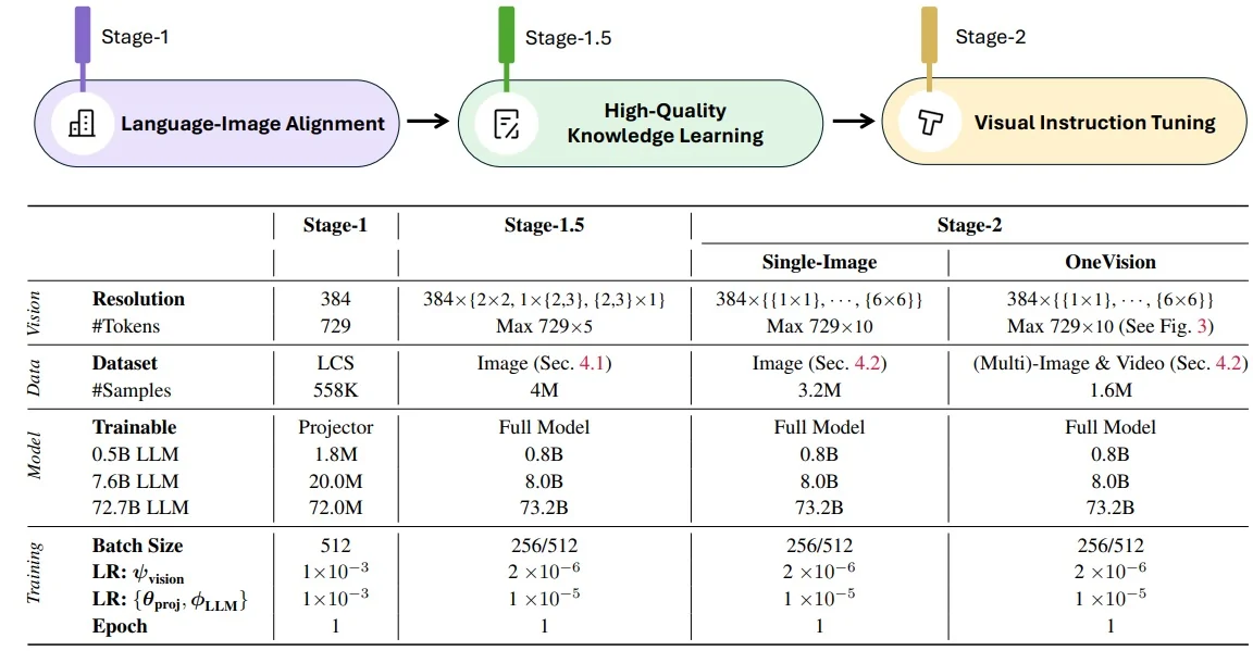
Data Collections (for SFT) LLaVA-OneVision adopts a two-stage instruction-tuning data design to first establish reliable single-image instruction-following “habits” and then extend those habits to multi-image and video. The sizing is deliberate: a large, diverse single-image corpus (to saturate core skills and stabilize alignment) followed by a leaner, mixed-modality corpus (to induce transfer without eroding single-image strength). This sequencing pairs naturally with the model recipe: Stage 2a focuses on breadth and fidelity under Higher AnyRes, while Stage 2b emphasizes cross-scenario generalization under balanced token budgets [335].
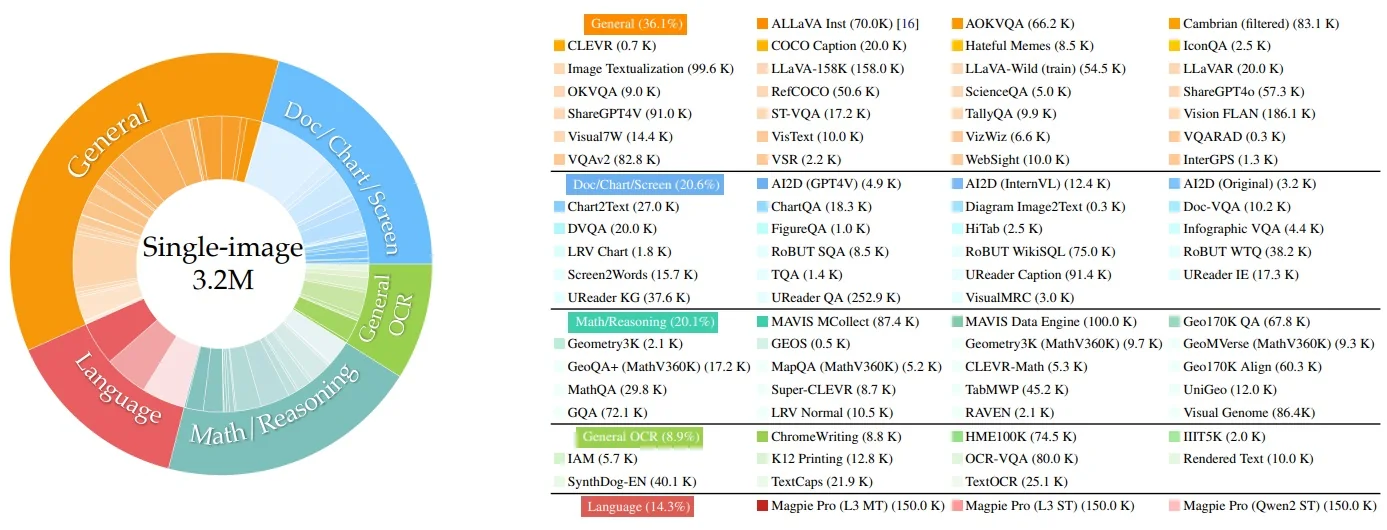
Why 3.2M single-image first? Single images are the richest, cleanest supervision for teaching the model to follow instructions while handling high-resolution details (documents, charts, UI, fine OCR) and structured reasoning (math, multi-step answers). This scale reduces sparsity across categories and prevents overfitting to any one task format. Practically, it lets the projector+LLM see consistent, high-fidelity tokens (via Higher AnyRes) across many domains, so later scenarios can reuse these routines (scan, localize, read, reason) rather than learn them from scratch.
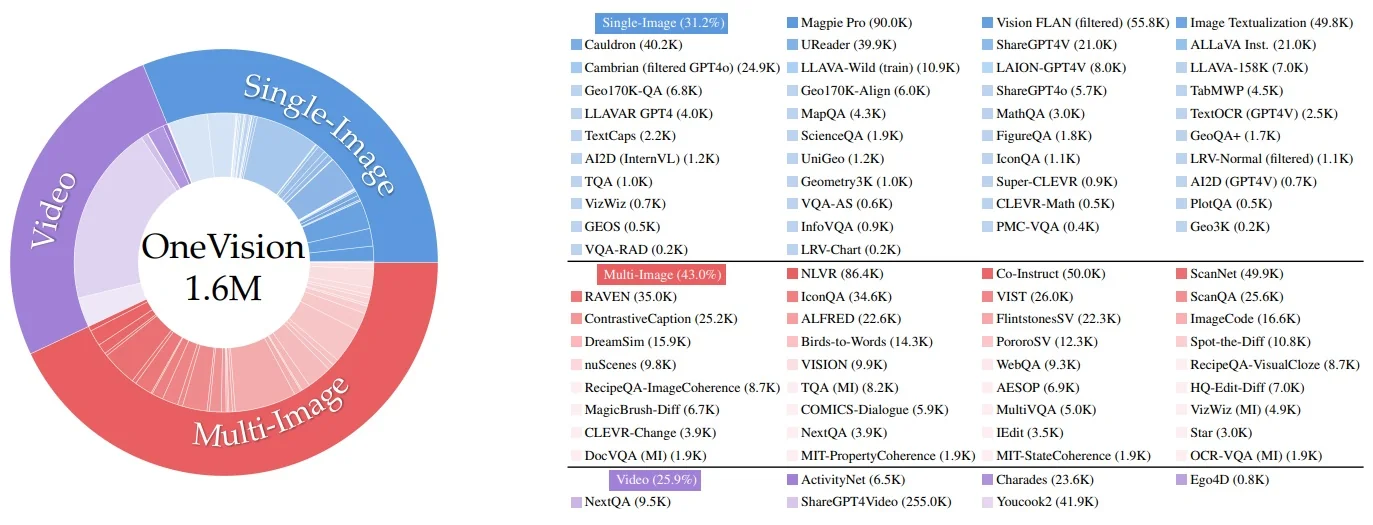
Why a smaller 1.6M mixed set next? After consolidating single-image skills, the model is exposed to multi-image (cross-view comparison, set reasoning) and video (temporal ordering, change detection) while still seeing some single-image refreshers. Keeping this stage smaller maintains the single-image baseline and avoids “washing out” its high-resolution gains. Crucially, the mixed set is curated to align with modality-parity constraints: a tiled high-res image, a small image set, and a short frame sequence occupy comparable visual-token budgets. This forces the LLM to apply shared routines (scan \(\rightarrow \) compare \(\rightarrow \) summarize/locate changes) across modalities, which is the mechanism behind the observed cross-scenario transfer [335].
Takeaway. The 3.2M single-image corpus builds a dependable instruction-following core with high-res fidelity; the 1.6M mixed corpus then “teaches the model to generalize” by practicing the same routines across set and temporal inputs under a unified token budget. The figures summarize the scale and composition that make this two-stage strategy effective [335].
Experiments & Ablations
What the Experiments Show The experiments confirm that LLaVA-OneVision achieves state-of-the-art open-source performance across modalities, rivaling GPT-4V on more than 70% of benchmarks. For example, the 7B model reaches 56.8% on MMMU (college-level multi-discipline QA), tying GPT-4V on this difficult evaluation [335]. Several key insights emerge:
- Unified capability. Skills acquired in one modality transfer to others. Single-image (SI) models retain \(\sim \)90% of full performance on ActivityNet-QA (video action QA), while mixed (SI+MI+video) SFT pushes multi-image VQA to 90.2% (7B), \(\sim \)20 points higher than LLaVA-NeXT’s interleaving baseline. Logical reasoning also scales: NLVR2 accuracy reaches 89.4%, a \(\sim \)10% gain over BLIP-2’s static image-only training.
- Native video QA. Sequential tokens with causal temporal attention outperform frame-interleaved baselines, improving VideoMME to 58.2% (7B), a +6.3% gain over GPT-4V (7B-equivalent). Balanced token budgets allow 32-frame clips without exploding inference cost, yielding strong conversational ratings (3.49/5) close to GPT-4V (4.06).
- High-resolution perception. AnyRes and Higher AnyRes yield significant OCR/text improvements: DocVQA rises to 87.5% (+4.7% over LLaVA’s low-res), while ChartQA climbs +3–5%. On HierText, tiled inputs add +8% retrieval recall, preserving fine text cues absent in downsampled BLIP-2/InstructBLIP.
Compared to priors:
- LLaVA excelled on static diagrams (e.g., 96.0% ScienceQA) but had no native video ability; OneVision adds +10–20% across video and multi-image benchmarks.
- BLIP-2 / InstructBLIP rely on Q-Former bridges for static image-text; they achieve \(\sim \)90% ScienceQA but collapse on dynamics. OneVision surpasses by +5–10% on video and multi-image QA without Q-Former overhead.
- SigLIP provided stronger image-text alignment (e.g., 79.1% ImageNet zero-shot); OneVision builds on this, adding +2–3% gains in document/ocr tasks.
Ablation Themes (High-Level) The ablations clarify which design choices matter most:
- Resolution handling. Removing Higher AnyRes drops text/small-object performance by 3–5% (e.g., TextVQA, ChartQA). Gains are sharpest on dense, text-heavy data (e.g., +8% on HierText). This validates tiling + global fusion as superior to the global resize used in LLaVA or BLIP-2.
- Token budget balance. Over-allocation to one modality reduces transfer (–5–10%). Balanced allocations (e.g., 12 images \(\approx \) 32 frames) stabilize training and improve generalization (+8–15% on MuirBench, a multi-image benchmark). This enforces shared reasoning routines, unlike unconstrained LLaVA sequences.
- Curriculum. Three-stage training (alignment \(\rightarrow \) knowledge \(\rightarrow \) instruction) outperforms end-to-end by +10–15% in convergence speed and stability. Mixed SI+MI+video SFT is essential: SI-only retains \(\sim \)90% on ActivityNet-QA, but adding video boosts EgoSchema (egocentric QA) by +10%. This extends InstructBLIP’s instruction tuning to dynamics without heavy architectural additions.
Qualitative Capabilities (Selected Examples)
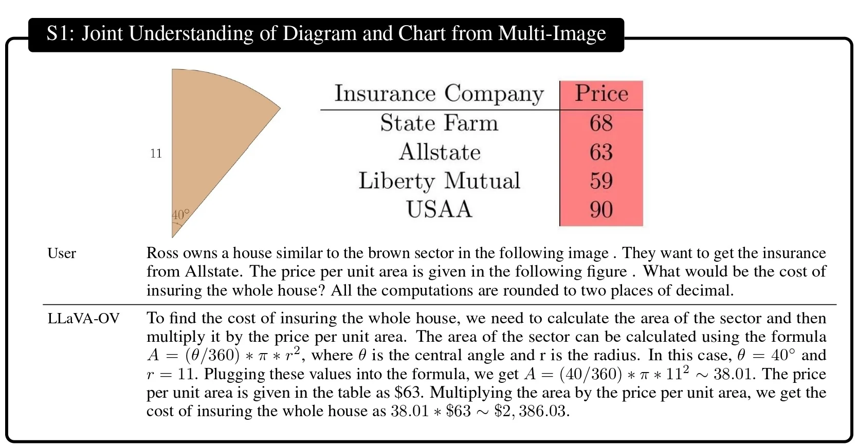
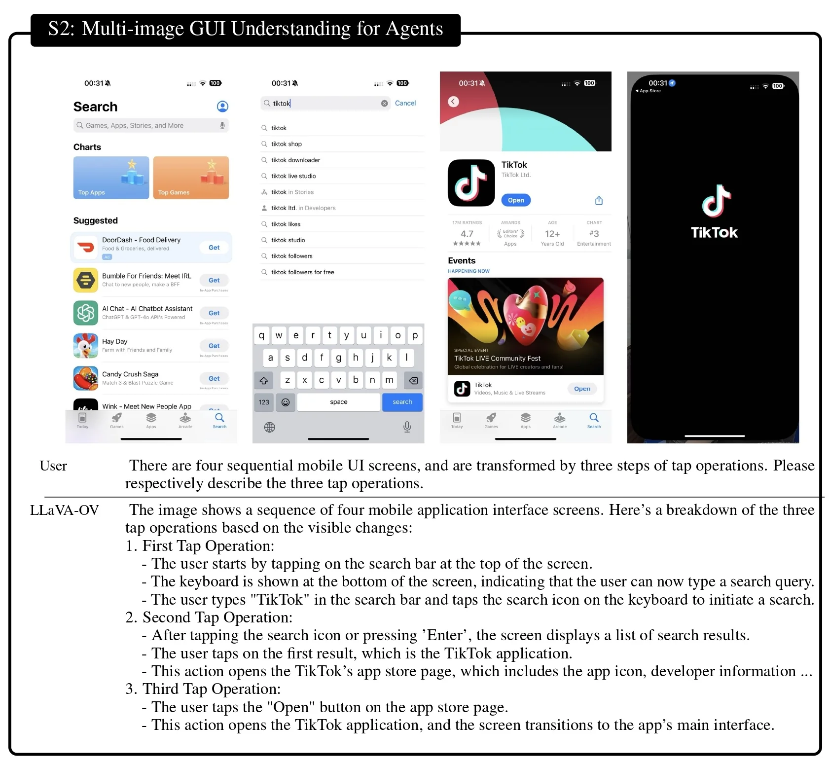

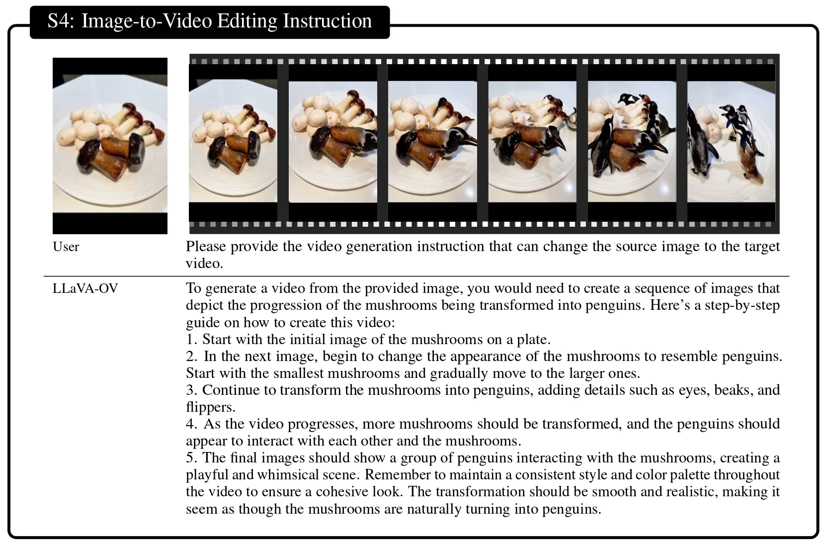
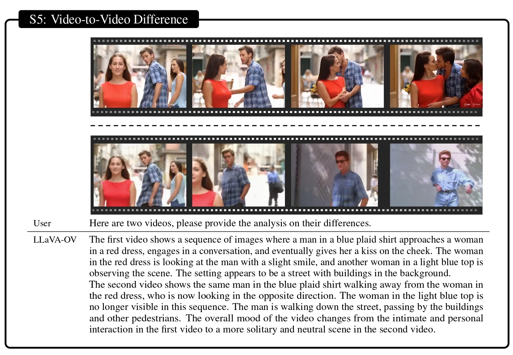
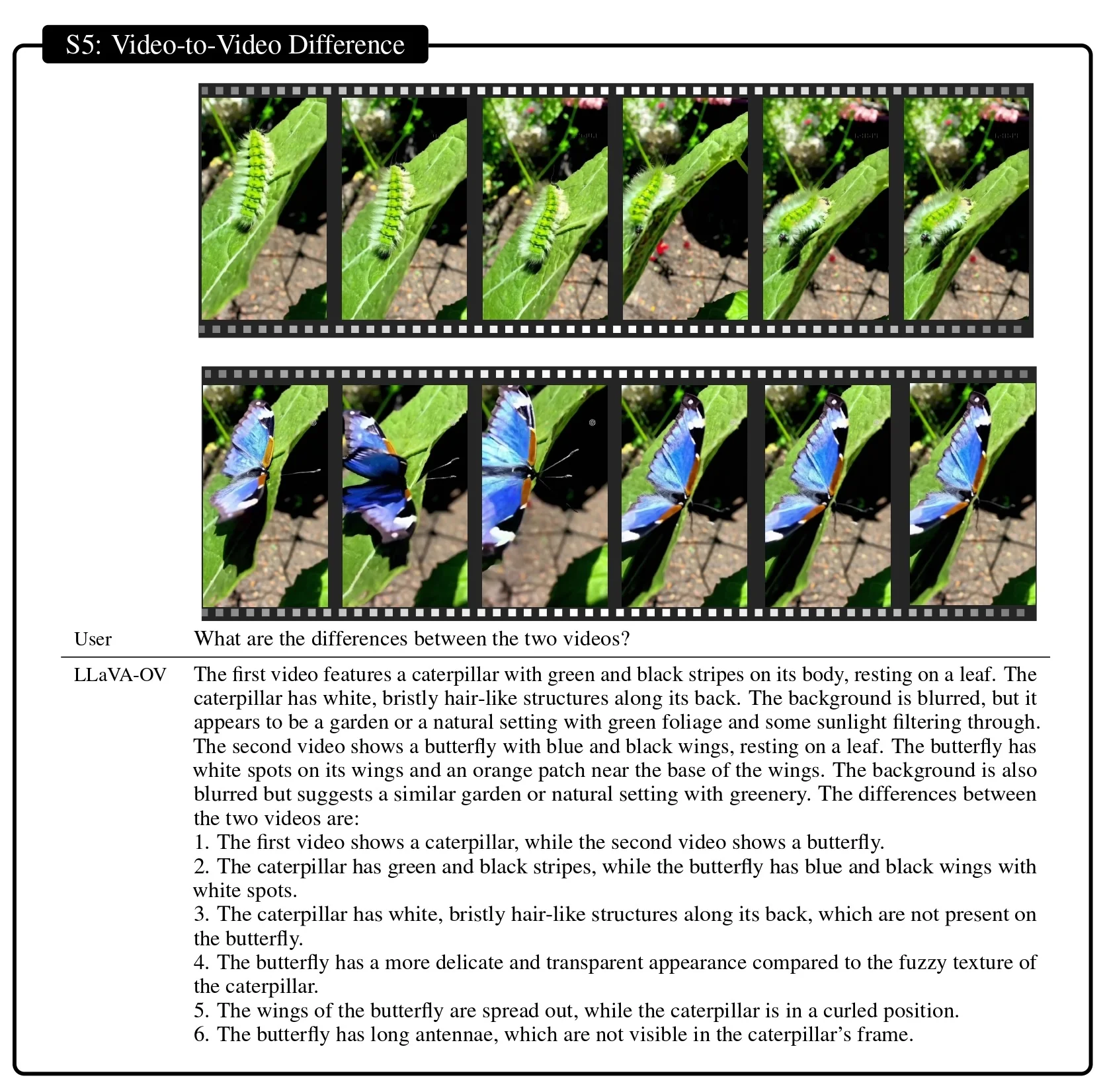
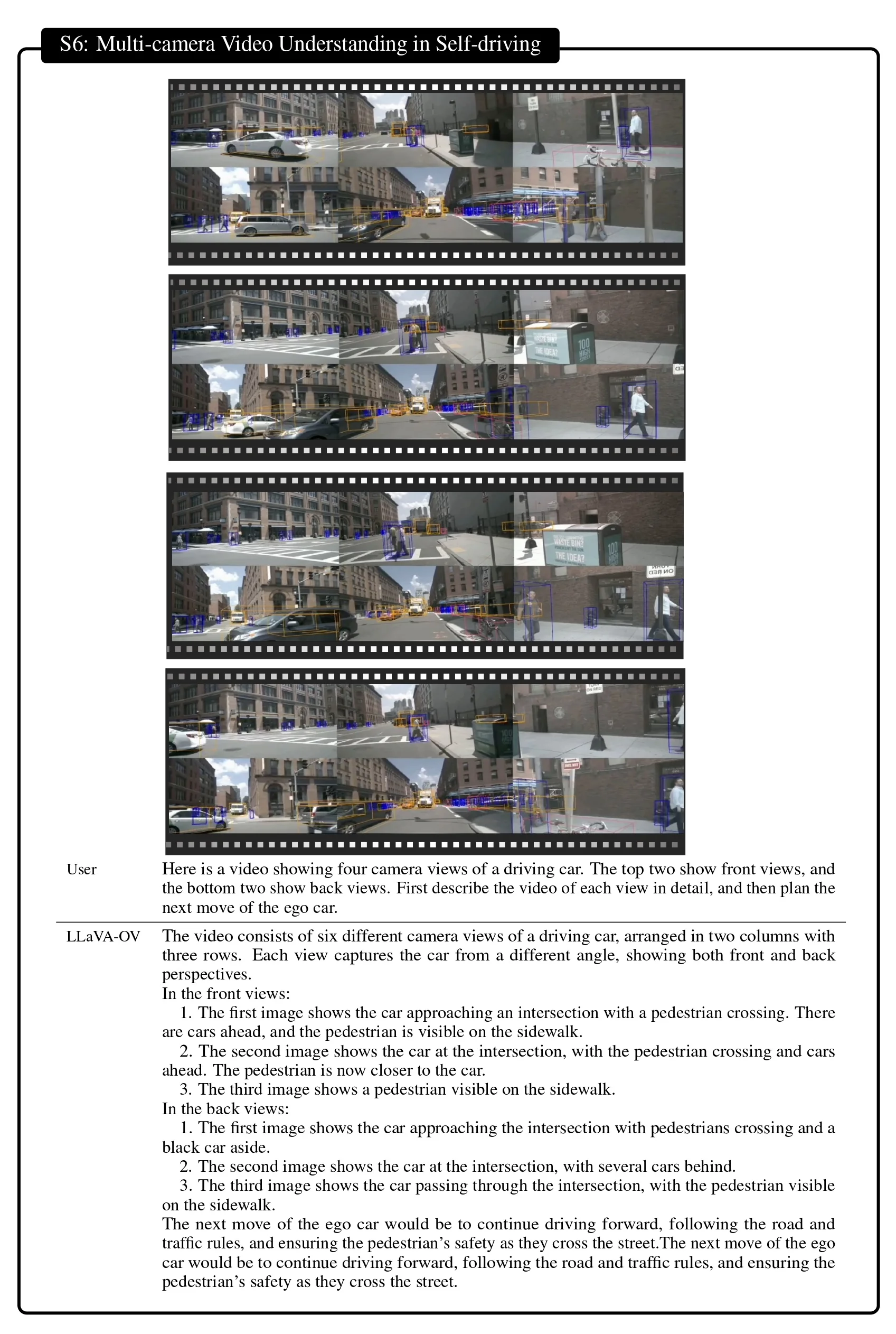
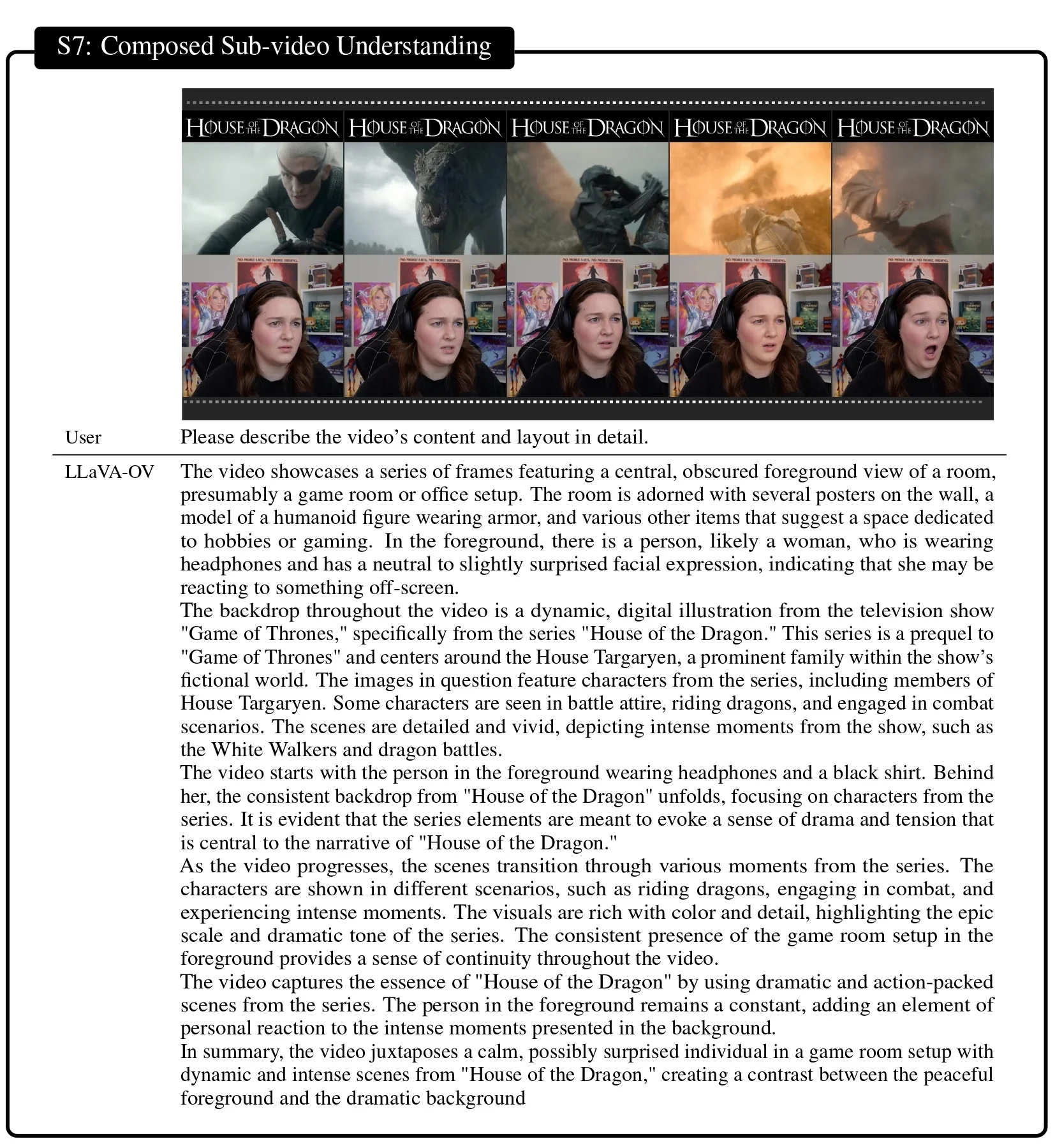
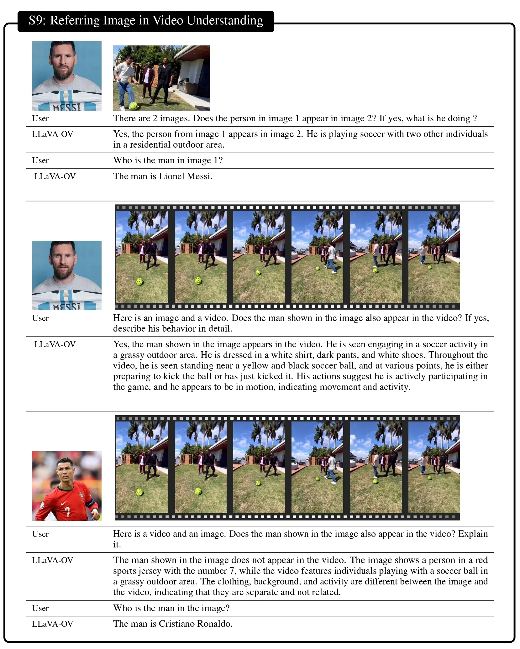
Limitations & Future Work
Current Constraints While LLaVA-OneVision (OV) set a new bar for open, unified multimodal models, its paper acknowledges several bottlenecks that limit generalization and accessibility:
- Compute & data appetite. Training OV-72B required a multi-stage curriculum over \(\sim \)9M samples, consuming weeks on large GPU clusters. This high entry cost restricted reproducibility and open adoption.
- Region semantics. AnyRes tiling preserved global context and high-res detail, but lacked explicit region-level modeling. As a result, dense OCR and document tasks plateaued (e.g., DocVQA 87.5%, \(\approx \)5% behind GPT-4o).
- Context budget. Although token parity across scenarios (single image \(\sim \) multi-image \(\sim \) short video) stabilized training, the fixed LLM window still capped long-form video and ultra-high-res image reasoning.
- Complex multimodal chat. Even at 72B scale, OV left a “relatively larger gap” in nuanced, conversational visual chat compared to proprietary models like GPT-4o.
Directions and the Move to OV-1.5 The follow-up LLaVA-OneVision-1.5 [10] was designed explicitly to overcome these issues, while retaining OV’s unified paradigm:
- Efficient, open training. OV-1.5 was trained from scratch under a \(\$16\)k compute budget via offline data packing and hybrid parallelism, compressing the pipeline to \(\sim \)1 week on 128\(\times \)A800s. This democratizes access, making large-scale multimodal training reproducible for the community.
- Richer vision front-ends. OV’s AnyRes encoder was replaced with RICE-ViT, a region-aware backbone pretrained on 450M images / 2.4B regions. This improves fine-grained semantics, boosting OCRBench by +5% (80.0%) and DocVQA to 95.0%, narrowing the gap with GPT-4o.
- Balanced, large-scale data. OV-1.5 introduced an 85M concept-balanced pretrain set and a 22M instruction set, covering broader domains and reducing biases. Ablations show +5–10% gains on multi-discipline QA (e.g., MMBench) compared to OV’s original 9M.
- Performance at smaller scale. New 4B/8B models (Qwen3 backbone) surpass Qwen2.5-VL-7B on 18/27 benchmarks, with the 4B even beating Qwen2.5-VL-3B on all 27. This means OV-1.5 achieves parity with or beyond proprietary closed models at a fraction of cost.
Future Directions Looking ahead, several paths are clear:
- Extending RICE-ViT. Adding temporal encoders or adaptive token selection to RICE-ViT could further lift long-video QA and dense OCR tasks, beyond OV-1.5’s gains.
- Scaling with balance. Expanding the 85M pretraining corpus to hundreds of millions of multimodal samples—while preserving concept balance—would improve cross-domain generalization and reduce bias.
- Tool grounding. Integrating external OCR engines, retrieval, or diagram solvers offers a hybrid route to bridge factuality gaps in specialized domains like math, forms, or charts.
In sum, LLaVA-OneVision introduced a unified recipe, but remained compute-heavy and limited in fine-grained reasoning. LLaVA-OneVision-1.5 directly addressed these pain points with efficient training, region-aware vision, and balanced data scaling, providing a stronger open foundation and paving the way toward even richer multimodal reasoning at scale.
Enrichment 24.8: Large-Scale Video Foundation Models
Web-scale pretraining yields general-purpose video encoders usable across recognition, detection, and retrieval. We outline InternVideo [693] and InternVideo2 [700]—scaling data, architectures, and objectives—and OmniVL [683], a unified image–video–language model. Related and emerging directions span mixture-of-experts backbones, multi-resolution clip sampling, and unified pretraining across video and audio.
Enrichment 24.8.1: InternVideo: General Video Backbones
Scope and positioning InternVideo [693] is a large-scale video foundation recipe that couples generative masked video modeling with discriminative multimodal contrastive learning and coordinates the two through a lightweight Cross-Model Attention (CMA) head. The design yields a representation that transfers broadly to action understanding, video–language alignment (supervised and zero-shot), and open-world video tasks, surpassing both specialized and prior foundation baselines.
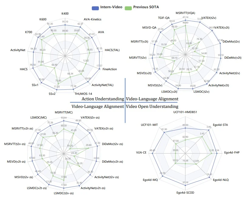
Motivation
Large-scale video pretraining has been led by two complementary paradigms:
- Masked Video Modeling (MVM). Epitomized by VideoMAE (see Sec. Enrichment 24.5.4), MVM reconstructs heavily masked spatiotemporal tubelet tokens without labels to learn motion-aware representations that transfer well to action understanding and localization (e.g., TAL: Temporal Action Localization; STA: Spatio-Temporal Action localization). However, because it lacks explicit language grounding, it does not natively support video–language tasks such as VQA (Video Question Answering) or cross-modal retrieval T2V/V2T (Text-to-Video / Video-to-Text), unless sizable supervised heads or additional alignment training are introduced.
- Vision–Language Contrastive Learning (CLIP-style). This paradigm aligns a video encoder with a text encoder via an InfoNCE objective, thereby endowing models with semantics and strong zero-shot transfer on video–language tasks like VQA and cross-modal retrieval T2V/V2T, and also aiding instruction-following settings such as VLN (Vision-and-Language Navigation). Yet when an image-pretrained ViT is naïvely extended to video, temporal structure can be under-exploited, weakening fine motion modeling and long-range dynamics for core video understanding and localization tasks (e.g., TAL/STA).
InternVideo addresses these complementary gaps by separately pretraining a strong masked video encoder (for motion/appearance coherence) and a strong multimodal video encoder (for language-aligned semantics), and then coordinating them at adaptation time through a lightweight Cross-Model Attention (CMA) fusion. In the intermediate CMA modules, masked-video (VideoMAE) spatiotemporal tokens serve as Queries, while multimodal (video–language) tokens provide Keys and Values, transferring semantic context into the masked path. In the final CMA module, the multimodal class token serves as the Query over masked-video tokens as Keys/Values, yielding an enriched video–language token used for prediction [693].
What InternVideo solves and how. InternVideo [693] proposes a dual-path recipe plus a lightweight coordination mechanism that combine the strengths of both worlds:
- Two specialized pretraining paths. A masked video encoder is trained generatively (as in VideoMAE; Sec. Enrichment 24.5.4) to capture spatiotemporal dynamics; in parallel, a multimodal video encoder with a text encoder is trained discriminatively with contrastive (and captioning) objectives to acquire language-grounded semantics [693]. Pretraining the two paths separately avoids the optimization friction of joint, multi-loss training.
- Coordination at adaptation time. After pretraining, InternVideo freezes the two encoders and learns a small Cross-Model Attention (CMA) head that lets the multimodal encoder’s class token query fine-grained tokens from the masked encoder. This fuses semantic abstraction with detailed motion/appearance evidence, improving over MVM-only approaches (e.g., VideoMAE/VideoMAEv2) by adding language awareness and over contrastive-only models by injecting robust temporal cues [693].
- A stronger video backbone on the multimodal path. To ensure the multimodal branch is temporally competent, InternVideo adopts UniFormer [347] / UniFormerV2 [355] as the vision backbone, which explicitly handle temporal redundancy and long-range space–time dependencies while preserving powerful image-pretrained priors (details below). These preliminaries are essential because they explain why the multimodal path already outputs motion-aware visual tokens that align well with text and how CMA can then query complementary, reconstruction-trained tokens from the masked path.
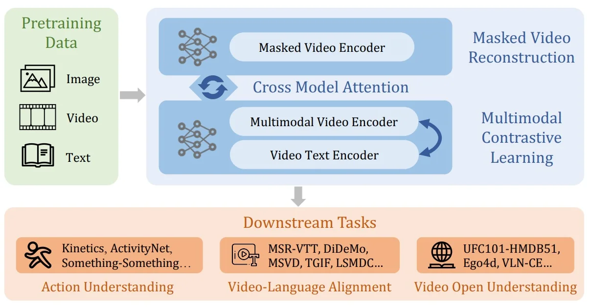
Preliminaries: UniFormer and UniFormerV2
Why these preliminaries matter here. Readers familiar with VideoMAE (Sec. Enrichment 24.5.4) already understand the masked path that InternVideo pretrains generatively. The multimodal path must pair clean language alignment with a video backbone that satisfies the following.
- Early temporal efficiency: Suppress short-range temporal redundancy early to control compute while retaining motion cues.
- Long-range coherence: Preserve strong long-range space–time reasoning so actions and events remain coherent over many frames.
- Stable reuse of image priors: Reuse powerful image-pretrained ViT priors without destabilizing them, enabling strong spatial semantics and rapid convergence.
UniFormer [347] and UniFormerV2 [355] meet these requirements, explaining why InternVideo’s contrastive branch is already motion-aware before CMA fusion and why CMA can effectively transfer semantics and dynamics between the two pretrained branches.
UniFormer (CVPR’22) [60] Block structure. Given a clip token tensor \(\boldsymbol {X}_{\mbox{in}}\!\in \!\mathbb {R}^{C\times T\times H\times W}\), a UniFormer block applies Dynamic Position Embedding (DPE), Multi-Head Relation Aggregator (MHRA), and an FFN with residuals: \begin {align} \boldsymbol {X} &= \mathrm {DPE}(\boldsymbol {X}_{\text {in}}) + \boldsymbol {X}_{\text {in}}, \label {eq:uni_dpe}\\[1mm] \boldsymbol {Y} &= \mathrm {MHRA}(\mathrm {Norm}(\boldsymbol {X})) + \boldsymbol {X}, \label {eq:uni_mhra_uniformer}\\[1mm] \boldsymbol {Z} &= \mathrm {FFN}(\mathrm {Norm}(\boldsymbol {Y})) + \boldsymbol {Y}. \label {eq:uni_ffn_uniformer} \end {align}
For relation learning, the spatiotemporal grid \((T,H,W)\) is flattened into a token sequence \(\boldsymbol {X}\in \mathbb {R}^{L\times C}\) with \(L=T\!\times \!H\!\times \!W\). A UniFormer block then proceeds in the fixed order \[ \mbox{DPE} \;\longrightarrow \; \mbox{MHRA} \;\longrightarrow \; \mbox{FFN}, \] with residual connections and normalization at each step. Why this order? DPE first injects local, learnable spatiotemporal bias so tokens “know” relative offsets; MHRA then aggregates context using either cheap local relations (early) or expressive global attention (late); the FFN finally refines per-token channels. This mirrors the progression from biasing \(\to \) mixing \(\to \) refining, which is stable and compute-efficient for video.
Dynamic Position Embedding (DPE): learnable relative spatiotemporal bias. DPE applies a depthwise 3D convolution to the token grid and adds it back as a residual: \begin {align} \boldsymbol {X} &= \mathrm {DPE}(\boldsymbol {X}_{\text {in}}) + \boldsymbol {X}_{\text {in}}, \qquad \mathrm {DPE}(\boldsymbol {X}_{\text {in}})=\mathrm {DWConv}(\boldsymbol {X}_{\text {in}}). \label {eq:uni_dpe_def} \end {align}
Intuition. Unlike absolute (or fixed sinusoidal) position embeddings that inject static coordinates, DPE transforms features with learned \(3{\times }3{\times }3\) per-channel kernels, encoding relative offsets in time and space. Because the convolution is depthwise, each channel learns its own stencil: motion-sensitive channels can emphasize temporal neighbors \((\Delta t=\pm 1)\), while appearance channels can emphasize spatial neighbors \((\Delta h,\Delta w)\). This yields translation-friendly, length-agnostic positional cues and lets different channels specialize without interfering. DPE thus “primes” tokens with local geometry before any relation mixing.
Why not just add absolute time/space codes? What is gained by DPE?
- Robust to augmentations. Absolute codes are brittle under temporal cropping, frame-rate changes, and resizing; DPE learns relative offsets that transfer across clip lengths and sampling strides.
- Local early cues. Early layers chiefly need local position signals (edges, small motions). A learned \(3\mathrm {D}\) stencil injects these directly without hard-coding coordinates.
- Channel-wise specialization. Depthwise filters let different channels emphasize temporal or spatial offsets (or anisotropic mixes), which a single shared absolute code cannot provide.
- Subtle absolute hints. Zero padding at boundaries yields weak “start/end” cues while keeping the representation predominantly relative.
MHRA (general form): one template that adapts with depth. After normalization, MHRA aggregates context per head via an affinity matrix \(\boldsymbol {A}_n\) and value projection \(\boldsymbol {V}_n\): \begin {align} \boldsymbol {Y} &= \mathrm {MHRA}(\mathrm {Norm}(\boldsymbol {X})) + \boldsymbol {X}, \label {eq:uni_mhra} \\[-1mm] \boldsymbol {R}_n(\boldsymbol {X}) &= \boldsymbol {A}_n\,\boldsymbol {V}_n(\boldsymbol {X}), \qquad \mathrm {MHRA}(\boldsymbol {X})=\mathrm {Concat}\big (\boldsymbol {R}_1;\dots ;\boldsymbol {R}_N\big )\,\boldsymbol {U},\ \boldsymbol {U}\in \mathbb {R}^{C\times C}. \label {eq:uni_mhra_general} \end {align}
Intuition. Each head chooses where to look through \(\boldsymbol {A}_n\) and what to bring through \(\boldsymbol {V}_n\). The same template becomes either local (kernel-like) or global (self-attention) by instantiating \(\boldsymbol {A}_n\) differently.
MHRA—Local (shallow stages): cheap neighborhood mixing. In early layers, \(\boldsymbol {A}_n\) is a learnable tubelet kernel restricted to a small neighborhood \(\Omega ^{t\times h\times w}_i\) around token \(i\): \begin {equation} A_{n}^{\mathrm {local}}(\boldsymbol {X}_i,\boldsymbol {X}_j)=a^{\,n}_{\,i-j}, \qquad j\in \Omega ^{t\times h\times w}_i,\quad a^{\,n}\in \mathbb {R}^{t\times h\times w}. \label {eq:uni_local} \end {equation}
MHRA—Local - why here and why effective.
- From quadratic to (near) linear cost. Full self-attention at shallow depth compares all token pairs and costs \(\mathcal {O}(L^2)\) with \(L=T\!\times \!H\!\times \!W\), which is prohibitively large before any downsampling. Constraining interactions to a fixed local tube \(\Omega \) of size \(t\!\times \!h\!\times \!w\) replaces \(\mathcal {O}(L^2)\) with \(\mathcal {O}(L\cdot thw)\). Since \(t,h,w\) are small constants, this is effectively \(\mathcal {O}(L)\), cutting both compute and memory drastically.
- Matches the signal statistics in video. Adjacent frames and neighboring patches are highly redundant in early layers; most useful cues are short-range (edges, micro-motions). A local stencil aggregates exactly these signals without paying for far-away comparisons that rarely help at low-level stages.
- Efficient, learnable, and specialized. The kernel \(a^{n}\) is learned end-to-end and reused at every location, behaving like a per-head depthwise 3D convolution (akin to a PW–DW–PW block). Different heads can specialize to distinct temporal spans or spatial orientations, capturing short hand trajectories, lip motions, or local texture changes with minimal overhead.
Takeaway. Local MHRA provides the right tool at the right place: it compresses short-range redundancy and builds robust low-level spatiotemporal features at (near) linear cost, reserving expensive global reasoning for deeper layers where sequence length is smaller and semantics are richer.
MHRA—Global (deep stages): full space–time self-attention when it counts. In deeper layers, \(\boldsymbol {A}_n\) becomes content-adaptive self-attention over all tokens: \begin {equation} A_{n}^{\mathrm {global}}(\boldsymbol {X}_i,\boldsymbol {X}_j)= \frac {\exp \big (Q_n(\boldsymbol {X}_i)^\top K_n(\boldsymbol {X}_j)\big )} {\sum _{j'\in \Omega ^{T\times H\times W}}\exp \big (Q_n(\boldsymbol {X}_i)^\top K_n(\boldsymbol {X}_{j'})\big )}. \label {eq:uni_global} \end {equation} Why later. Global attention is quadratic in \(L\), but by the time features are deep and (typically) downsampled, \(L\) is smaller and semantics are richer. This is when modeling long-range dependencies—linking distant frames, disambiguating similar motions via scene context, tracking multi-object interactions—pays off most, matching the “cheap local early, expressive global late” principle from efficient video networks.
FFN: per-token refinement. A position-wise MLP (with expansion and contraction) follows to refine channels: \begin {equation} \boldsymbol {Z}=\mathrm {FFN}(\mathrm {Norm}(\boldsymbol {Y})) + \boldsymbol {Y}. \label {eq:uni_ffn} \end {equation} Role. MHRA mixes between tokens; FFN mixes within a token’s channels to build nonlinear feature compositions (e.g., fusing motion edges and object cues).
Putting it together: why this staging works for video.
- Bias then mix. DPE injects learnable relative geometry so tokens carry local spatiotemporal context before any aggregation, improving stability and translation-friendliness.
- Local then global. Local MHRA removes short-range redundancy inexpensively and locks onto micro-motion early; global MHRA later provides clip-level reasoning exactly where semantic abstraction and reduced \(L\) make it most useful and affordable.
- Refine per token. The FFN consolidates mixed evidence into compact, discriminative channels, preparing features for the next stage or for global fusion blocks downstream.
Concrete cue. Consider “opening a door”—a pattern combining subtle, short-range hand–handle interactions with a larger, long-range door-panel swing. UniFormer’s staging processes this in three steps:
- DPE — inject relative spatiotemporal order. Motion-sensitive channels privilege temporal neighbors (capturing tiny wrist twists), while edge/texture channels privilege spatial neighbors (sharpening handle contours). This primes tokens with local geometry before relation mixing.
- Local MHRA + FFN — assemble robust local cues at low cost. Local MHRA mixes only within a small 3D neighborhood, stitching a few-frame wrist–handle trajectory with nearby edges at near-linear cost; the subsequent FFN performs pointwise nonlinear refinement, amplifying the fused “grasp–twist” cue and suppressing noise.
- Global MHRA + FFN — resolve long-range semantics. Deep global MHRA performs full space–time attention, linking the refined local cue to door-panel motion across the clip and to body pose evolution; a final FFN consolidates this global evidence into a discriminative token.
Outcome. The representation separates “opening a door”—sustained forward rotation and panel displacement—from lookalikes such as “touching a handle” (no panel displacement) or “closing a door” (opposite temporal signature), with early stages handling redundant micro-dynamics efficiently and later stages resolving long-range semantics accurately.
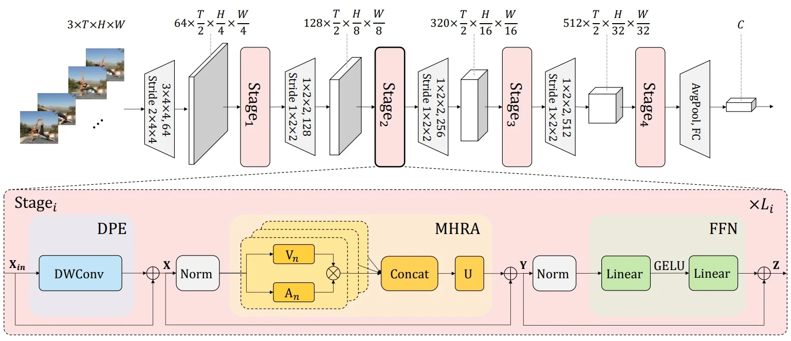
From UniFormer (V1): what we gained, and what still needs fixing.
- What V1 achieved. It unified cheap local relations early with expressive global attention late (via MHRA + DPE), cutting shallow-layer cost, reducing redundancy, and improving long-range reasoning for actions—yielding a strong accuracy–FLOPs trade-off for video transformers.
- What V1 lacked. As a new backbone, it did not reuse powerful image-pretrained ViT weights; obtaining robust spatial priors required separate, sizable supervised image pretraining before video adaptation, increasing engineering and compute overhead.
- What V2 must fix next. Keep V1’s local\(\rightarrow \)global strengths while plugging into widely available image ViTs: add minimal temporal adapters for short-range dynamics, and lightweight global aggregators for clip-level context—so the model inherits strong 2D priors and efficient video modeling out of the box.
UniFormerV2 (ICCV’22) [104]: arming image ViTs for video, with full formulation and clear integration. Goal and integration at a glance. Start from an image-pretrained ViT and insert the smallest possible temporal machinery so that all strong spatial priors (attention weights, MLPs, and 2D positional encodings) are kept intact. Concretely:
- Keep (reuse) the ViT block as-is for space. The standard ViT multi-head self-attention and FFN (per frame) are retained, so pretrained spatial weights and 2D position embeddings load without change.
- Add a temporal adapter before each block. A lightweight Local Temporal MHRA (LT-MHRA) is attached in a residual, pre-norm form, mixing only along time at each spatial site. This leaves the original spatial attention unchanged but makes tokens temporally aware.
- Add cheap global video aggregation late. A Global UniBlock (one-query cross-attention) produces per-clip video tokens at selected deep layers; it is orthogonal to the ViT’s per-frame attention, so pretrained spatial weights remain unaffected.
Local UniBlock (LT-MHRA \(\rightarrow \) GS-MHRA \(\rightarrow \) FFN). Let \(\boldsymbol {X}^{\mbox{in}}\!\in \!\mathbb {R}^{L\times C}\) be tubelet tokens \((L=T\!H\!W)\). The block applies \begin {align} \boldsymbol {X}^{T} &= \mathrm {LT\_MHRA}\big (\mathrm {Norm}(\boldsymbol {X}^{\mbox{in}})\big ) + \boldsymbol {X}^{\mbox{in}}, \label {eq:uv2_lt}\\ \boldsymbol {X}^{S} &= \mathrm {GS\_MHRA}\big (\mathrm {Norm}(\boldsymbol {X}^{T})\big ) + \boldsymbol {X}^{T}, \label {eq:uv2_gs}\\ \boldsymbol {X}^{L} &= \mathrm {FFN}\big (\mathrm {Norm}(\boldsymbol {X}^{S})\big ) + \boldsymbol {X}^{S}. \label {eq:uv2_ffn} \end {align}
Here \(\mathrm {GS\_MHRA}\) is the original ViT spatial attention applied per frame (so its pretrained weights and 2D positional encodings are reused directly), while \(\mathrm {LT\_MHRA}\) is a new temporal adapter. The shared MHRA form follows Eq. (??).
LT-MHRA (temporal-local adapter). Temporal neighborhood only, per channel and per spatial site: \begin {equation} A^{\mbox{LT}}_{n}(\boldsymbol {X}_i,\boldsymbol {X}_j)=a^{\,n}_{\,i-j},\quad j\in \Omega ^{t\times 1\times 1}_i,\quad a^{\,n}\!\in \!\mathbb {R}^{t\times 1\times 1}. \label {eq:uv2_lt_aff} \end {equation} Why it fits. Adjacent frames are redundant; a depthwise 1D temporal conv (kernel \(t\!\approx \!3\)) captures short-range dynamics at \(\mathcal {O}(L\cdot t)\) cost, leaves spatial attention/FFN weights unchanged, and therefore preserves the pretrained ViT’s spatial priors.
GS-MHRA (spatial-global within a frame, weight reuse). Standard ViT attention applied per frame: \begin {equation} A^{\mbox{GS}}_{n}(\boldsymbol {X}_i,\boldsymbol {X}_j)= \frac {\exp \big (Q_n(\boldsymbol {X}_i)^\top K_n(\boldsymbol {X}_j)\big )} {\sum _{j'\in \Omega ^{1\times H\times W}}\exp \big (Q_n(\boldsymbol {X}_i)^\top K_n(\boldsymbol {X}_{j'})\big )}. \label {eq:uv2_gs_aff} \end {equation} Why it fits. This is exactly the pretrained image ViT’s spatial self-attention: keys/queries/values and 2D positional encodings are loaded as-is. Because temporal mixing happens before this step via LT-MHRA, the ViT can leverage its spatial priors on temporally enriched tokens without retraining from scratch.
Global UniBlock (one-query cross-attention \(\Rightarrow \) video tokens). At selected deep layers, \begin {align} \boldsymbol {X}^{C} &= \mathrm {DPE}(\boldsymbol {X}^{L}) + \boldsymbol {X}^{L}, \label {eq:uv2_dpe}\\ \boldsymbol {X}^{ST} &= \mathrm {C\_MHRA}\big (\mathrm {Norm}(\boldsymbol {q}),\,\mathrm {Norm}(\boldsymbol {X}^{C})\big ), \label {eq:uv2_cmhra}\\ \boldsymbol {X}^{G} &= \mathrm {FFN}\big (\mathrm {Norm}(\boldsymbol {X}^{ST})\big ) + \boldsymbol {X}^{ST}. \label {eq:uv2_g_ffn} \end {align}
with a single learnable query \(\boldsymbol {q}\!\in \!\mathbb {R}^{1\times C}\). Per head, \begin {align} \boldsymbol {R}^{\,C}_n(\boldsymbol {q},\boldsymbol {X}) &= \boldsymbol {A}^{\,C}_n(\boldsymbol {q},\boldsymbol {X})\,\boldsymbol {V}_n(\boldsymbol {X}), \\ A^{\,C}_n(\boldsymbol {q},\boldsymbol {X}_j) &= \frac {\exp \!\big (Q_n(\boldsymbol {q})^\top K_n(\boldsymbol {X}_j)\big )} {\sum _{j'\in \Omega ^{T\times H\times W}}\exp \!\big (Q_n(\boldsymbol {q})^\top K_n(\boldsymbol {X}_{j'})\big )}. \label {eq:uv2_cross} \end {align}
The output is one video token \(\boldsymbol {X}^G\!\in \!\mathbb {R}^{1\times C}\) per chosen depth (per clip). Why it fits. This is content-aware global pooling with \(\mathcal {O}(L)\) cost; it does not alter the pretrained per-frame attention weights and adds only a small number of parameters (query and projections), keeping the original ViT intact for spatial reasoning.
Multi-stage fusion (what is fused, where it plugs). Collect video tokens \(\{\boldsymbol {X}^G_i\}\) from several deep layers and fuse:
- Sequential: \(\boldsymbol {X}^G_i \!=\! \mathcal {G}_i(\boldsymbol {X}^G_{i-1},\boldsymbol {X}^L_i)\) progressively refines summaries.
- Parallel: \(\boldsymbol {F}=\mathrm {Concat}(\boldsymbol {X}^G_1,\dots ,\boldsymbol {X}^G_N)\,\boldsymbol {U}^F\) aggregates multi-scale semantics in one shot.
- Hierarchical (Q or KV): Propagate queries or keys/values across depths so later tokens condition on earlier summaries.
Finally, mix \(\boldsymbol {F}\) with the final class token via a learned gate, \(\boldsymbol {Z}=\alpha \,\boldsymbol {F} + (1-\alpha )\,\boldsymbol {F}^{C}\), yielding a compact clip descriptor. Why it fits. Shallow video tokens carry fine temporal cues; deeper ones carry semantics. Fusion balances both, while preserving the pretrained ViT’s spatial pathway.
Why this staging preserves pretrained weights and improves efficiency.
- Temporal adapter first. LT_MHRA mixes only along time in a residual path, leaving the ViT’s per-frame attention and FFN untouched; pretrained 2D weights and positional encodings load directly.
- Spatial path unchanged. GS_MHRA is the original ViT spatial attention applied within each frame; keys/queries/values and 2D position embeddings are reused without modification.
- Late, linear-cost globalization. The one-query Global UniBlock appears only in deep layers, providing clip-level context at \(\mathcal {O}(L)\) (vs. \(\mathcal {O}(L^2)\)) when features are already abstract.
Net effect. UniFormerV2 retains strong image-ViT spatial priors, adds minimal temporal mixing, and introduces inexpensive clip-level aggregation—exactly what InternVideo needs for temporally competent, language-alignable video features.
Concrete cue. For “pouring coffee”, LT_MHRA stabilizes micro-motions of mug and pot across adjacent frames; GS_MHRA relates hand, mug, and pot within each frame. In deep layers, a Global UniBlock extracts a video token that concentrates on the interval where liquid flow is visible despite camera shake. Finally, UniFormerV2 late-integrates this video token with the backbone’s [CLS] token via a learned gate (\(\boldsymbol {Z}=\alpha \,\boldsymbol {F}+(1{-}\alpha )\boldsymbol {F}^{C}\)), yielding a clip descriptor that fuses temporally pooled evidence (\(\boldsymbol {F}\)) with the strong spatial prior captured by [CLS] (\(\boldsymbol {F}^{C}\)). In InternVideo’s final CMA, the multimodal [CLS] further queries masked-video tokens, enriching this summary with fine motion/detail before task heads.
Bridging to the method: why UniFormer/UniFormerV2 set the stage.
- Temporally competent yet ViT-friendly. UniFormer/UniFormerV2 inject lightweight temporal mixing (LT_MHRA) before standard ViT spatial attention and keep the per-frame attention/FFN unchanged. This preserves strong 2D priors while yielding tokens that already encode short-range dynamics.
- Compact clip-level context. Late one-query cross-attention produces video tokens—content-aware summaries of the entire clip—that complement the usual [CLS] representation via a learned late integration. These summaries are ideal anchors for downstream fusion.
- Natural interface for cross-stream fusion. With temporally aware patch tokens, a robust [CLS] token, and per-clip video tokens, the backbone exposes clean query/key/value points. In the following, the method will leverage these to coordinate a generative (masked-reconstruction) stream and a discriminative (video–language) stream through lightweight cross-attention, transferring semantics and motion cues without retraining the backbones.
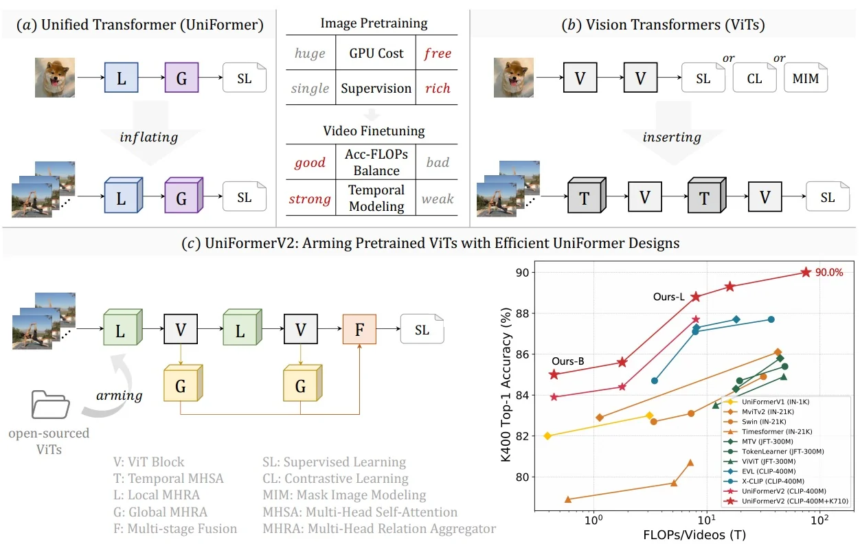
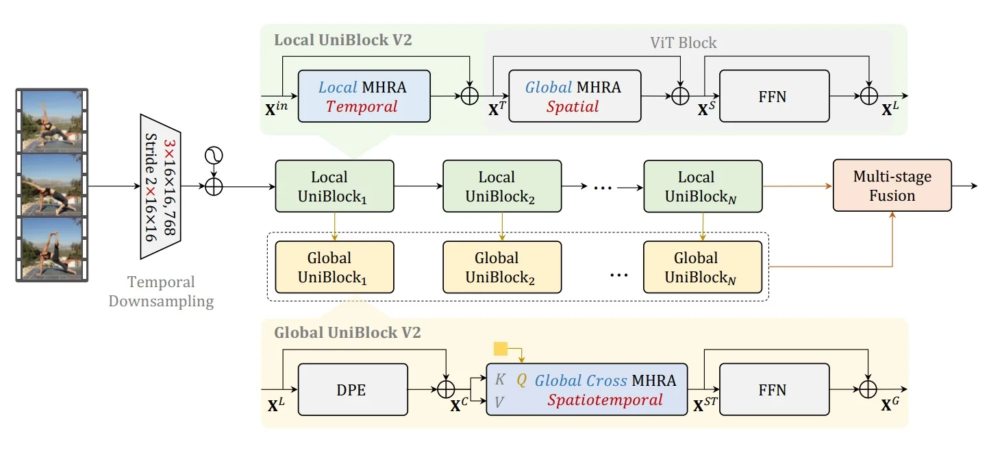
Method
High-level overview InternVideo trains two complementary encoders with different pretext signals and then coordinates them at adaptation time via lightweight cross-attention:
- Masked Video Encoder (MVE). VideoMAE-style ViT with high-ratio tube masking (\(\approx 90\%\)) and an asymmetric encoder–decoder that reconstructs pixels and learns motion/appearance-coherent features without labels.
- Multimodal Video Encoder (MMVE). UniFormerV2-based video backbone paired with a transformer text encoder, typically CLIP-initialized, trained on large-scale video/image–text data via a symmetric contrastive loss and a cross-modal captioning loss for language-aligned semantics [104, 101].
-
Coordination via Cross-Model Attention (CMA). After separate pretraining, both backbones are frozen and small cross-attention+FFN adapters are inserted so the streams can query each other [101]:
- Intermediate fusion: MVE tokens query MMVE tokens to absorb semantic structure (inject language-aligned cues into motion-rich features).
- Final fusion: MMVE [CLS] queries MVE tokens to inject precise motion/detail into the multimodal summary used for prediction.
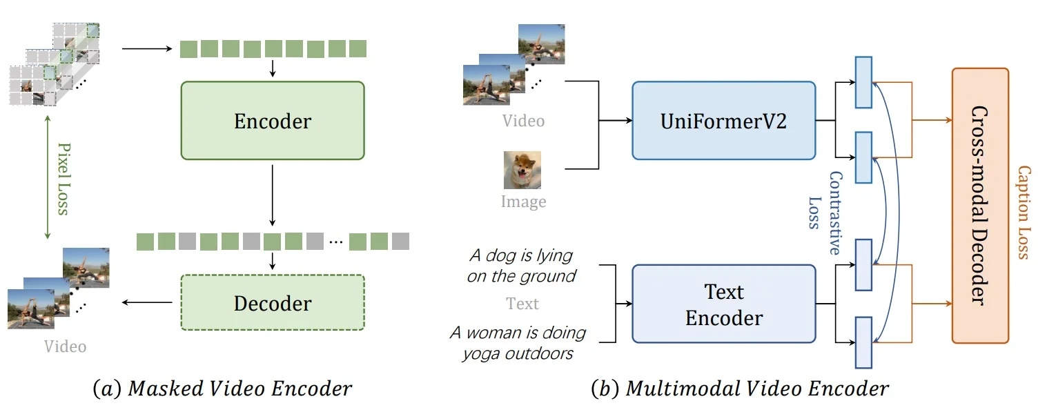
Notation Let a video clip be tokenized into tubelets and embedded as \(\boldsymbol {X}\!\in \!\mathbb {R}^{L\times C}\) with \(L=T\!\times \!H\!\times \!W\). Cosine similarity is \(\mathrm {sim}(\cdot ,\cdot )\). Temperatures are \(\tau >0\). The symbol \(\odot \) denotes elementwise multiplication.
1) Generative path — Masked Video Encoder (MVE) InternVideo adopts a VideoMAE-style asymmetric ViT for self-supervised masked video pretraining:
- Tube masking. A large fraction (e.g., 90%) of spatiotemporal tubelet tokens is masked; only visible tokens are processed by the encoder, making joint space–time attention computationally tractable on long clips.
- Asymmetric encoder–decoder. A compact decoder (fewer channels/blocks) reconstructs the original pixels (or low-level targets) from the encoder features and mask tokens.
Pixel reconstruction loss. With ground-truth pixel targets \(\boldsymbol {Y}\) and reconstruction \(\hat {\boldsymbol {Y}}\), the masked-patch regression uses mean-squared error over masked positions: \begin {equation} \mathcal {L}_{\mbox{pix}} \;=\; \frac {1}{|\mathcal {M}|}\sum _{p \in \mathcal {M}}\big \|\hat {\boldsymbol {Y}}_{p}-\boldsymbol {Y}_{p}\big \|_2^{2}, \label {eq:internvideo_pix} \end {equation} where \(\mathcal {M}\) indexes masked tubelets. This forces the encoder to form motion/appearance-coherent, temporally aware features that predict missing content from sparse context.
2) Discriminative path — Multimodal Video Encoder (MMVE) InternVideo builds on CLIP-style alignment but uses UniFormerV2 as the video backbone (Sec. 24.8.1.0), paired with a transformer text encoder and a small cross-modal caption decoder:
- Align before fuse. First align video and text embeddings with a symmetric contrastive loss; then fuse them using a decoder with cross-attention under a captioning loss. This brings zero-shot alignment (retrieval) and stronger multimodal composition (caption/VQA) in a single framework [101, 104].
Contrastive loss. Given minibatch \(\{(\boldsymbol {v}_i,\boldsymbol {t}_i)\}_{i=1}^{B}\) of video/text embeddings, \begin {align} \mathcal {L}_{\mbox{v}\rightarrow \mbox{t}} &= -\frac {1}{B}\sum _{i=1}^{B} \log \frac {\exp \big (\mathrm {sim}(\boldsymbol {v}_i,\boldsymbol {t}_i)/\tau \big )} {\sum _{j=1}^{B}\exp \big (\mathrm {sim}(\boldsymbol {v}_i,\boldsymbol {t}_j)/\tau \big )}, \\ \mathcal {L}_{\mbox{t}\rightarrow \mbox{v}} &= -\frac {1}{B}\sum _{i=1}^{B} \log \frac {\exp \big (\mathrm {sim}(\boldsymbol {t}_i,\boldsymbol {v}_i)/\tau \big )} {\sum _{j=1}^{B}\exp \big (\mathrm {sim}(\boldsymbol {t}_i,\boldsymbol {v}_j)/\tau \big )}, \\ \mathcal {L}_{\mbox{con}}&=\frac {1}{2}\left (\mathcal {L}_{\mbox{v}\rightarrow \mbox{t}}+\mathcal {L}_{\mbox{t}\rightarrow \mbox{v}}\right ). \label {eq:internvideo_contrast} \end {align}
Captioning loss: concise mechanics and intuition Each training clip is paired with a ground-truth caption (GT) from the video–text dataset. The model does not predict “video tokens”; it predicts the next word token in the caption.
Who is Query/Key/Value—and why. In a transformer caption decoder, the text prefix ([BOS] \(w_1,\dots ,w_{t-1}\)) forms the queries: the decoder is asking, “given the words so far, what visual evidence do I need next?” The video features produced by the UniFormerV2 encoder (dense spatiotemporal tokens and optional video tokens from Global UniBlocks) serve as keys/values: they are the searchable memory of what happened where and when. Cross-attention thus retrieves the relevant visual context to emit the next word.
How training proceeds. With teacher forcing, the decoder conditions on the ground-truth prefix and predicts the next word; the token-level cross-entropy \[ \mathcal {L}_{\mathrm {cap}} \;=\; -\sum _{t=1}^{T_{\mbox{cap}}} \log p_\theta (w_t \mid w_{<t},\,\mbox{video}) \] is minimized. The overall multimodal objective combines retrieval-oriented alignment and generative grounding: \[ \mathcal {L}_{\mathrm {MM}} \;=\; \mathcal {L}_{\mathrm {con}} \;+\; \lambda _{\mathrm {cap}}\mathcal {L}_{\mathrm {cap}} ,\qquad \lambda _{\mathrm {cap}}>0. \]
Why this design works.
- Queries from text. Language dictates what detail is needed next (object \(\rightarrow \) attribute \(\rightarrow \) action), so using the textual prefix as queries makes the decoder “ask” targeted questions of the video memory.
- Keys/values from video. UniFormerV2 provides (i) dense tokens for fine, localized evidence (hands, objects, micro-motions) and (ii) video tokens—compact, late-stage summaries—for long-range context (phases of an action). This mix lets cross-attention retrieve both sharp details and global storyline.
- What “video token” means. It is a learned, per-clip summary feature (one token per selected deep layer), not a word to predict. The decoder can attend to it alongside dense tokens to maintain temporal coherence in generation.
- Why add captioning to contrastive. Contrastive loss aligns whole video–text pairs (useful for retrieval), but captioning forces word-by-word grounding: to emit each token, the decoder must attend to the correct frames/regions. This strengthens VQA/captioning and makes retrieval more robust to distribution shift.
Role of UniFormerV2 (video memory). LT_MHRA compacts short-range motion (clean verb cues), GS_MHRA preserves strong spatial priors (reliable nouns/attributes), and Global UniBlocks add per-clip summary tokens (temporal coherence). Together they produce a video memory that the decoder can query precisely—rich in detail yet resistant to spurious shortcuts.
3) Coordination — Cross-Model Attention (CMA). Setup. After the masked and multimodal paths are pretrained independently, InternVideo freezes both backbones and inserts a small stack of CMA adapters at selected mid/high layers [693]. Each adapter is a residual, post-norm block with multi-head cross-attention (MHCA) followed by an FFN. Let \[ \mathrm {MHCA}(\boldsymbol {Q},\boldsymbol {K},\boldsymbol {V})=\mathrm {Concat}(\mathrm {head}_n)\,\boldsymbol {W}_o,\qquad \mathrm {head}_n=\mathrm {softmax}\!\Big (\tfrac {\boldsymbol {Q}\boldsymbol {W}^Q_n(\boldsymbol {K}\boldsymbol {W}^K_n)^{\!\top }}{\sqrt {d}}\Big )\,(\boldsymbol {V}\boldsymbol {W}^V_n). \] The host stream supplies queries \((\boldsymbol {Q})\) and is updated; the guest stream supplies keys/values \((\boldsymbol {K},\boldsymbol {V})\) as read-only memory. Lightweight \(1{\times }1\) projections inside the adapter align channel widths when needed.
Directional use (who queries whom, and why).
- Intermediate CMA (MVE \(\rightarrow \) MMVE). At several early/mid depths of the masked path, MVE tokens are used as \(\boldsymbol {Q}\) and MMVE tokens as \(\boldsymbol {K},\boldsymbol {V}\). The adapter output replaces (or is residually added to) the MVE tokens. Effect: transfers language-aligned semantics into motion/appearance-coherent features while preserving their temporal precision.
- Final CMA (MMVE cls \(\rightarrow \) MVE). Just before the multimodal head, the MMVE class token is \(\boldsymbol {Q}\) and the full MVE token map is \(\boldsymbol {K},\boldsymbol {V}\). The updated class token becomes the input to the prediction head. Effect: injects fine motion/detail cues into the multimodal summary at decision time.
Why this placement.
- Preserve priors. Freezing both encoders protects pixel-reconstruction priors (MVE) and CLIP/UniFormerV2 priors (MMVE); CMA learns to align, not to overwrite [693].
- Parameter- and compute-efficient. Only the small adapter parameters \(\{\boldsymbol {W}^Q,\boldsymbol {W}^K,\boldsymbol {W}^V,\boldsymbol {W}_o\}\) and FFN are trained for a few supervised epochs; cross-attention cost scales with \(\mathcal {O}(L_{\!Q}L_{\!K})\) and remains modest at mid/high stages.
- Complementarity made explicit. Intermediate CMA semantically enriches motion-rich tokens; final CMA sharpens the language summary with precise dynamics, improving action understanding, retrieval, captioning, and VQA.
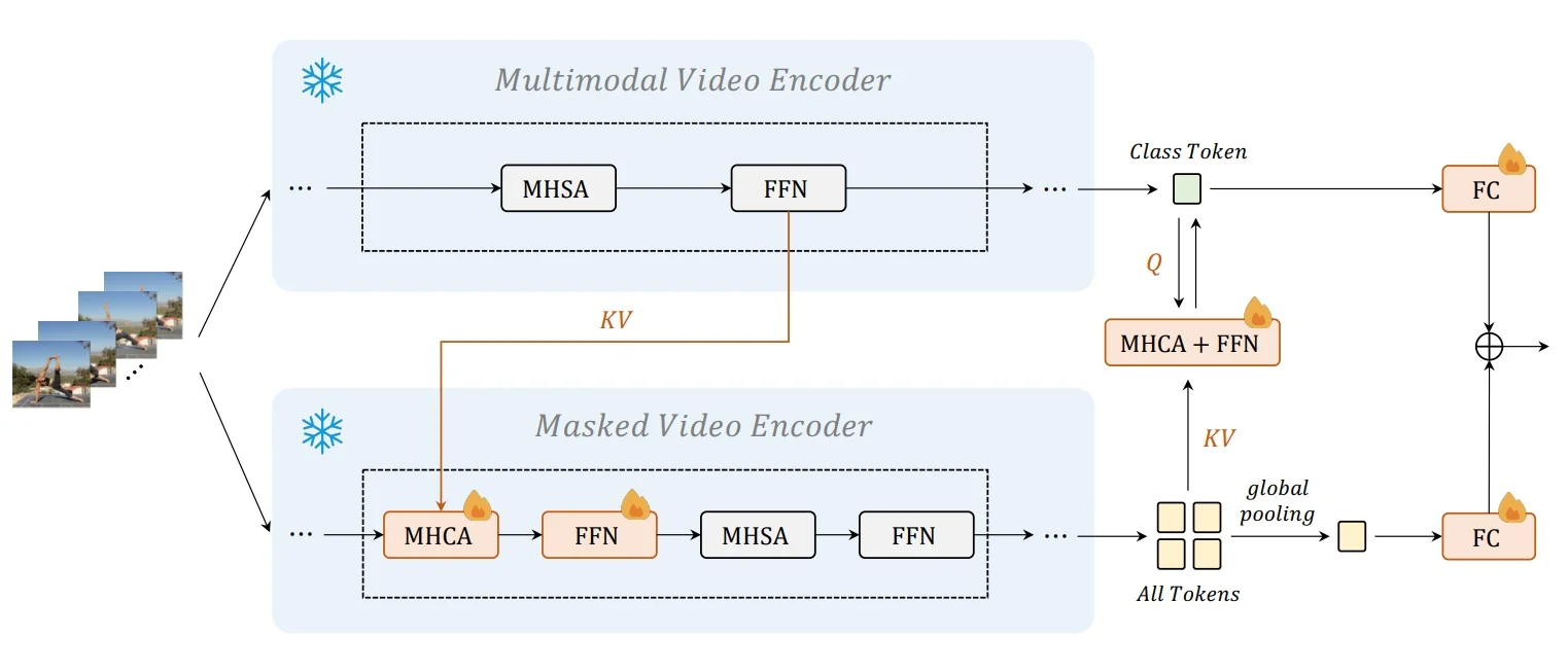
4) Prediction heads and supervised adaptation For action recognition, temporal localization, retrieval, and VQA/captioning, InternVideo attaches modest heads on top of the fused features:
- Recognition/localization. A linear/MLP head over the final fused token(s) (or task-specific proposals) trained with cross-entropy/mAP losses, depending on the benchmark setup.
- Retrieval. For text-to-video (T2V) and video-to-text (V2T), the aligned MMVE pathway enables using contrastive similarity between the fused video representation and text embeddings.
- VQA/caption. The cross-modal decoder (already trained) can be adapted with task supervision; CMA improves the video-side evidence entering the decoder.
The adaptation schedule used in the paper freezes both encoders and learns CMA (and the task heads) for a few epochs, providing a tractable path to fuse large pretrained models [693].
- 1.
- Two encoders (frozen at adaptation).
- (a)
- MVE: encode visible tubelets, decode reconstruction, providing masked-stream tokens.
- (b)
- MMVE (UniFormerV2 + text): encode video and text; obtain aligned embeddings and, optionally, decoder features.
- 2.
- CMA stacks. Apply intermediate CMA blocks with \(\boldsymbol {Q}=\) MVE tokens, \(\boldsymbol {K},\boldsymbol {V}=\) MMVE tokens; update MVE-side representations.
- 3.
- Final CMA. Use MMVE class token as \(\boldsymbol {Q}\) and MVE tokens as \(\boldsymbol {K},\boldsymbol {V}\); update the class token.
- 4.
- Heads. Feed the fused token(s) to the task head: classifier, retrieval similarity, localization head, or decoder.
Architecture and Implementation Details
- Masked Video Encoder (MVE) ViT with tubelet embedding and an asymmetric decoder as in VideoMAE; high mask ratio (\(\rho \!\approx \!0.9\)) for efficient joint space–time learning of visible tokens.
- Multimodal Video Encoder (MMVE) UniFormerV2 (Sec. 24.8.1.0) as the video tower and a transformer text tower (typically CLIP-initialized), paired with a lightweight caption decoder.
Tokenization and shapes A clip of \(T\) frames at resolution \(H{\times }W\) is patchified with temporal stride \(s_t\) and spatial stride \(s\) into \(T'\!\times \!H'\!\times \!W'\) tubelets, forming \(L=T'H'W'\) tokens of width \(C\). The MVE processes only the visible subset; the MMVE processes all tokens.
UniFormerV2 block order in MMVE Each block applies \(\mbox{LT_MHRA} \rightarrow \mbox{GS_MHRA} \rightarrow \mbox{FFN}\), preserving the pretrained ViT’s spatial attention and MLP while adding a residual temporal adapter At selected deep layers, a Global UniBlock (one-query cross-attention) emits video tokens (one per chosen depth), which serve as compact per-clip summaries for captioning and heads.
Cross-Model Attention (CMA) placement
- Intermediate CMA Inserted at several mid-depth stages along the MVE; \(\boldsymbol {Q}\) from MVE tokens, \(\boldsymbol {K},\boldsymbol {V}\) from MMVE tokens; output replaces or is residually added to MVE tokens.
- Final CMA Right before the MMVE head; \(\boldsymbol {Q}\) is the MMVE [CLS], \(\boldsymbol {K},\boldsymbol {V}\) are the full MVE token map; the updated [CLS] goes to prediction heads.
Each CMA adapter is a residual, post-norm MHCA\(+\)FFN; optional \(1{\times }1\) projections align channel widths.
- 1.
- Stage 1 Self-supervised masked pretraining of MVE with pixel regression over masked tubelets.
- 2.
- Stage 2 Multimodal pretraining of MMVE with symmetric contrastive alignment and captioning under teacher forcing; UniFormerV2 supplies temporally competent video features.
- 3.
- Stage 3 Supervised adaptation on downstream tasks with both encoders frozen; train only CMA and task heads.
Experiments and Ablations
Bottom-line summary across tasks
- Action recognition. On Kinetics-400/600/700, InternVideo attains 91.1/91.3/84.0% top-1 with billion-scale backbones (InternVideo-D/T), edging strong generative and multimodal pretraining baselines such as MaskFeat-L, CoCa, and MTV-H at comparable or larger scales [693, 710, 764, 742].
- More AR benchmarks. Gains transfer broadly: 70.0% on SthSthV1 (\(+9.1\)), 77.2% on SthSthV2 (\(+1.6\)), 94.3% on ActivityNet (\(+4.1\)), 95.5% on HACS (\(+3.6\)), and 89.3% on HMDB51 (\(+1.7\)) over prior best reports [693].
- Temporal localization. Coupled with strong heads, InternVideo improves average mAP on THUMOS-14, ActivityNet-v1.3, HACS, and FineAction; e.g., with ActionFormer it reaches 71.58 on THUMOS-14 and 39.00 on ActivityNet-v1.3, and with TCANet it reaches 41.55 on HACS [693, 783, 733].
- Spatiotemporal localization. With a linear head, InternVideo reports 41.01 mAP on AVA2.2 and 42.51 mAP on AVA-Kinetics, surpassing prior ensembles and MaskFeat while using minimal task-specific tuning [693, 479, 356, 710].
- Text–video retrieval. R@1 improves consistently over CLIP-derived baselines across MSR-VTT, MSVD, LSMDC, ActivityNet, DiDeMo, and VATEX for both T2V and V2T, reflecting stronger alignment and compositional grounding [693, 414, 421, 393].
- VQA and captioning. Adding a captioning objective yields absolute gains of \(\sim \)3–8 points on MSRVTT, MSVD, and TGIF, indicating that generative grounding complements contrastive alignment [693, 333, 163, 777, 676].
- Navigation and robustness. Improvements extend to VLN-CE and open-set AR, with higher success rates and better uncertainty calibration than prior backbones [693].
Key ablations and what they imply
- CMA matters. Removing cross-model attention lowers action recognition and retrieval, most notably for categories needing both fine motion and semantics, confirming stream complementarity and the benefit of two-direction fusion [693].
- Fusion directions are not interchangeable. Using only MVE\(\rightarrow \)MMVE or omitting the late MMVE [CLS]\(\rightarrow \)MVE step underperforms; the final class-token query is particularly important for recognition and retrieval [693].
- Mask ratio vs. clip length. Very high masking on short clips can over-regularize the MVE; tuning \(\rho \) jointly with clip length \(T\) stabilizes learning and improves transfer [693].
- Why UniFormerV2. Replacing UniFormerV2 with a naïve ViT video tower weakens captioning/VQA and retrieval under shift, underscoring the benefit of LT_MHRA and late video tokens for temporal coherence [355, 693].
- Scale with structure beats raw scale. InternVideo-T surpasses 1B+ baselines like CoCa and MTV-H on Kinetics despite similar or larger parameter counts, pointing to the benefits of structured dual pretraining and CMA over size alone [693, 764, 742].
- Complementary objectives help. Improvements on retrieval and VQA mirror the combination of \(\mathcal {L}_{\mbox{con}}\) and \(\mathcal {L}_{\mbox{cap}}\), while AR and localization gains show that motion structure learned by the MVE remains intact after coordination [693].
Limitations and Follow-up Works
- Two-tower rigidity. With encoders frozen at adaptation, CMA aligns mid/high-level features but has limited ability to influence early representations or permit full co-adaptation [693].
- Cross-attention budget. CMA complexity scales with \(L_Q L_K\); very long clips, high resolutions, or dense token maps can raise adaptation cost even if it remains lighter than end-to-end joint training.
- Temporal skew. Differences in sampling policies or augmentations between streams may introduce small frame misalignments unless clip timing is carefully synchronized.
- Language priors. Contrastive pretraining can reflect dataset caption biases; the captioning objective and CMA help, but residual bias may remain.
- Gentle co-adaptation. Move beyond fully frozen fusion by selectively or gradually unfreezing blocks around CMA sites, so motion and semantics can co-evolve while preserving strong pretrained priors.
- Token economy. Reduce the number of tokens entering CMA via dynamic pruning or routing, focusing cross-attention on salient motion regions and text-relevant evidence to keep \(L_Q,L_K\) modest.
- Stronger temporal bias. Improve temporal synchronization and long-horizon stability with richer relative position modeling and more reliable per-clip summary tokens, mitigating drift across long sequences.
- Unified curricula. Coordinate masking ratios, clip lengths, and the balance of masked, contrastive, generative losses—together with cleaner temporal segmentation and caption quality—to smooth optimization at scale.
Takeaway InternVideo indicates that separate generative and multimodal pretraining, followed by lightweight cross-attention coordination, can produce broadly transferable video representations across recognition, localization, retrieval, VQA, navigation, and open-set evaluation, and subsequent variants soften the two-tower boundary and streamline fusion cost while retaining the pretrained priors that underpin these gains [693].
Enrichment 24.8.2: OmniVL: One Model for Image–Video–Language
Scope and positioning OmniVL’s [683] central thesis is unification along three axes: data (image/video paired with either text or labels), modality (a single visual encoder for images and videos), and functionality (alignment and generation) without task-specific adapters. The authors introduce a decoupled joint curriculum and a Unified Vision–Language Contrastive loss (UniVLC) to couple clean labels with noisy captions, yielding bidirectional gains for both image and video tasks.
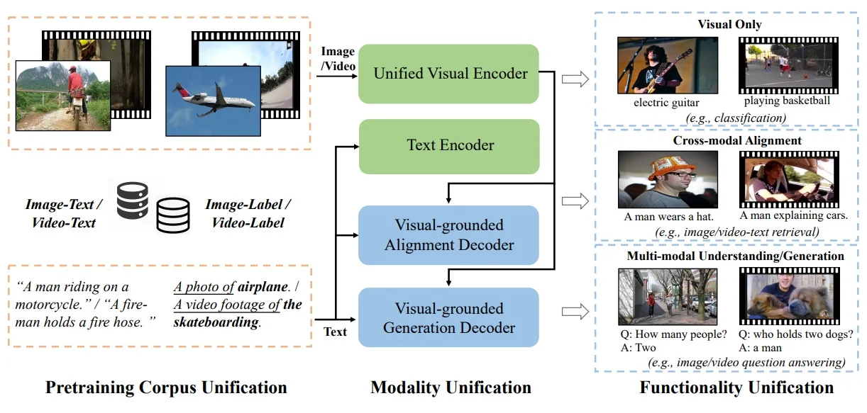
Motivation
Fragmentation problem The OmniVL paper [683] is motivated by persistent fragmentation in vision–language foundations, which hampers transfer, scalability, and simplicity of deployment. Three silos are especially limiting.
- Functionality silo (retrieval vs. generation). Many systems dedicate separate models or heavy adapters to non-generative alignment tasks (e.g., retrieval) versus generative tasks (e.g., captioning and QA), preventing a single representation from serving both effectively.
- Modality silo (image vs. video). Image-language models are often extended to video as independent frames or via ad-hoc heads, weakening temporal modeling and requiring extra parameters to adapt to motion.
- Data-source silo (captions vs. labels). Training on either clean, discriminative label corpora (e.g., ImageNet, Kinetics) or noisy, webly image/video–text pairs yields features that are respectively precise or broad but rarely both, leaving potential gains from joint supervision unrealized.
In practice, these silos force multiple specialized pipelines and miss beneficial cross-task and cross-modal transfer, particularly for video where temporal dependencies are essential.
Design hypothesis OmniVL posits that a single model can break these silos by unifying data, modality, and functionality under one pretraining and inference framework.
- Unified feature space via mixed supervision. Combining clean label corpora with webly caption corpora in a shared contrastive space should yield features that are simultaneously discriminative and semantically rich, improving both visual-only recognition and cross-modal understanding.
- Efficient spatio-temporal modeling in one encoder. Sharing a TimeSformer-style visual backbone across images and videos leverages strong spatial pretraining for images while activating temporal attention only for videos, avoiding duplicate encoders and encouraging transfer from spatial to spatio-temporal representation.
- Decoupled joint pretraining for stability and bidirectional gains. First learning on image–language to establish robust spatial representations, then continuing with joint image+video training, should introduce temporal dynamics without catastrophic forgetting and produce gains that flow in both directions (image \(\leftrightarrow \) video).
This hypothesis underlies OmniVL’s choice of losses and curriculum, aiming to replace fragmented stacks with a single foundation that scales across tasks and modalities.
Method: high-level flow and detailed breakdown
High-level overview OmniVL [683] follows an encoder–decoder design that routes the same inputs through a unified pipeline and learns three complementary objectives. The end-to-end flow is: tokenizing \(\rightarrow \) positional encodings (spatial, temporal) \(\rightarrow \) unified visual encoder \(\rightarrow \) text encoder \(\rightarrow \) two visual-grounded decoders for alignment and generation \(\rightarrow \) task heads and objectives. A two-stage, decoupled joint pretraining curriculum first builds strong spatial representations on image–language, then introduces video–language to learn temporal dynamics while preserving the spatial foundation. This structure supports visual-only tasks, cross-modal alignment, and multi-modal generation within a single model without task-specific adapters.
Data format and prompting All pretraining sources are expressed in a joint visual–label–text space [683]. Each sample is a triplet \(S=(x,y,t)\), where \(x\) is an image or a video, \(y\) is a unique category index, and \(t\) is its language description. For image/video–label data, \(t\) is generated with CLIP- and ActionCLIP-style prompt templates by filling class names, so that all visual samples with the same category share a common textual description. This formulation unifies four corpora: image–text, video–text, image–label, and video–label.
- 1.
- Tokenizing. Raw inputs are converted into a unified token sequence suitable for a transformer. For an image \(x\!\in \!\mathbb {R}^{H\times W\times 3}\), OmniVL applies a 2D patch tokenizer implemented as a convolution with kernel and stride \(p\times p\), producing \(N=\tfrac {HW}{p^2}\) patch tokens in \(\mathbb {R}^{D}\) plus a learned [CLS] token. For a video \(x\!\in \!\mathbb {R}^{T\times H\times W\times 3}\), OmniVL uses a 3D tubelet tokenizer with kernel and stride \(\tau \times p\times p\) to yield \(N'=\tfrac {T}{\tau }\cdot \tfrac {HW}{p^2}\) tokens that already encode short-term motion, again prepending a [CLS]. Using dedicated 2D/3D tokenizers aligns the channel dimension \(D\) across modalities, injects a mild local inductive bias, and normalizes the interface to the shared encoder while allowing flexible frame sampling and tubelet length during training and fine-tuning [683].
- 2.
- Positional encodings. Self-attention is permutation invariant, so OmniVL injects position using learned, factorized absolute embeddings that separate space and time [683]. Let \(E_{\mathrm {s}}(h,w)\in \mathbb {R}^{D}\) be a learned spatial table on the 2D grid and \(E_{\mathrm {t}}(t)\in \mathbb {R}^{D}\) a learned temporal table on the 1D frame/tubelet axis. An image token at \((h,w)\) is \[ z_{0}^{h,w} \;=\; \mathrm {patch\_emb}\!\left (x^{h,w}\right ) \;+\; E_{\mathrm {s}}(h,w), \] and a video tubelet token at time \(t\), location \((h,w)\) is \[ z_{0}^{t,h,w} \;=\; \mathrm {tubelet\_emb}\!\left (x^{t,h,w}\right ) \;+\; E_{\mathrm {s}}(h,w) \;+\; E_{\mathrm {t}}(t). \] Why learned (vs. sinusoidal or purely relative). (i) Compatibility with image pretraining. The decoupled-joint schedule initializes the unified encoder from strong image checkpoints that use learned absolute PEs; keeping learned \(E_{\mathrm {s}}\) preserves this interface, easing transfer from Stage 1 (images) to Stage 2 (videos). (ii) Modality unification and weight sharing. A shared 2D spatial table \(E_{\mathrm {s}}\) across images and videos keeps the spatial grid consistent, so the same encoder weights can process both, while time is injected only when present via \(E_{\mathrm {t}}\). (iii) Stable scaling via interpolation. Factorizing space and time avoids a monolithic 3D table tied to fixed \((T,H,W)\); learned \(E_{\mathrm {s}},E_{\mathrm {t}}\) are smoothly interpolated for new resolutions or clip lengths at fine-tuning. (iv) Empirical simplicity. Learned absolute PEs are a lightweight, data-driven choice that match or outperform fixed sinusoids in ViT-style vision models while avoiding extra complexity in attention kernels required by some relative schemes. Overall, OmniVL’s learned, factorized PEs deliver the needed spatial layout and temporal order signals while aligning with the unified encoder and the training curriculum.
- 3.
- Unified visual encoder. A single transformer encoder with shared parameters processes both modalities. Each block follows a TimeSformer-style decoupled scheme, applying temporal self-attention across tokens at the same spatial index followed by spatial self-attention within each frame, with feed-forward layers and residual connections in between. For images, the temporal step is bypassed, so the encoder reduces to a ViT-like pathway; for videos, both temporal and spatial steps are active. Sharing almost all weights forces a common representational space where image-learned spatial semantics transfer to videos and video-learned temporal cues regularize spatial features. In the decoupled joint curriculum, Stage 1 trains this encoder on image–language data to solidify spatial features; Stage 2 continues training with mixed image+video batches to learn temporal dynamics without forgetting. The final hidden state of [CLS] serves as the global embedding \(v_{\mathrm {cls}}\) for recognition and retrieval, while the full token grid is exposed to the visual-grounded decoders via cross-attention for alignment and generation [683].
- 4.
- Text encoder. A transformer text encoder converts the tokenized caption or prompted label sentence into contextual embeddings, with a [CLS] token used for global text representation \(w_{\mathrm {cls}}\).
- 5.
- Visual-grounded decoders. Two transformer decoders fuse text with the
visual tokens for complementary functionalities while sharing the same
visual inputs [683]. Each decoder block follows the sequence self-attention \(\rightarrow \)
cross-attention to visual tokens \(\rightarrow \) feed-forward, with residual connections and
layer normalization throughout. The two decoders differ only in the
self-attention mask and the supervision signal, which is the crux of
unifying non-generative alignment and generative modeling in one
framework.
- Alignment decoder (non-generative). A special [ENC] token is prepended to the text sequence. The decoder uses bidirectional self-attention, which is the standard unmasked multi-head self-attention as in BERT encoders, so every text token can attend to every other token regardless of position to build a globally contextualized representation. After self-attention, each layer performs cross-attention with the text stream as queries and the visual token grid as keys/values, grounding the full sentence in the image or video content. The output embedding at [ENC] serves as a fused cross-modal representation that a linear head maps to a match probability for the Vision–Language Matching objective. In retrieval, encoder similarities shortlist candidates and this decoder re-ranks them using the [ENC] embedding, improving precision at low recall budgets.
- Generation decoder (generative). Architecturally mirrors the alignment decoder but replaces bidirectional self-attention with causal self-attention, implemented by a lower-triangular mask so token \(l\) only attends to positions \(\le l\). This makes the decoder autoregressive, which is necessary for text generation where future tokens must not leak into the current prediction. The text stream is wrapped with a [DEC] start token and an [EOS] end token and is trained with teacher forcing under the language modeling loss. Cross-attention at every layer conditions generation on the visual tokens, enabling captioning and question answering. At inference, the decoder generates tokens sequentially until [EOS] is emitted.
Causal vs. bidirectional in context. Bidirectional self-attention equals regular, unmasked MHSA and is ideal for understanding tasks that benefit from full-sequence context such as alignment and re-ranking, whereas causal self-attention enforces one-way information flow for generation by hiding future tokens, aligning supervision and attention with the autoregressive objective.
- 6.
- Contrastive memory banks. OmniVL casts pretraining as self-supervised contrastive learning to unify heterogeneous supervision at scale: paired image/video–text samples and class labels provide weak but ubiquitous signals, and contrastive SSL converts these co-occurrences into instance- and class-aware alignment across modalities without dense annotations. To obtain many, stable negatives, OmniVL adopts a MoCo-style momentum contrast [ref] [683]. Inputs are the current mini-batch of visual and text tokens. The online encoders produce query projections \((q_v,q_t)\), while momentum encoders—exponential moving average (EMA) copies—encode the same batch into keys \((k_v,k_t)\) updated by \[ \theta _{\mbox{mom}} \leftarrow m\,\theta _{\mbox{mom}} + (1-m)\,\theta _{\mbox{online}},\quad m\in [0,1) \] so targets change slowly and remain consistent across steps. Keys are stop-gradient and enqueued into fixed-capacity FIFO queues \(Q_v=\{v_m\}_{m=1}^{M}\), \(Q_t=\{w_m\}_{m=1}^{M}\) with labels \(Q_y=\{y_m\}_{m=1}^{M}\); oldest entries are dequeued to keep size \(M\). Computation of UniVLC uses the queues in InfoNCE denominators to supply thousands of negatives, and forms positives from the paired query–key as well as class-aware keys with \(y_k{=}y_i\), tying together image–text, video–text, image–label, and video–label signals in one objective. Why EMA and not large batches. SimCLR-style training would require very large synchronized batches to approximate this many negatives; EMA keys act as a slowly moving teacher that stabilizes the dictionary, prevents target drift when the online encoder updates, and enables a vast, cheap negative set via queues without increasing memory or cross-device synchronization. Outputs are stronger and smoother gradients for cross-modal alignment, leading to more robust representations under mixed corpora and improved optimization stability.
Pretraining objectives OmniVL learns three complementary skills in parallel—global alignment, pairwise verification, and conditional generation—so that one checkpoint can serve retrieval, recognition, and captioning/QA. The three losses operate on different heads but share the unified encoders, so gradients reinforce rather than conflict [683].
Unified Vision–Language Contrastive (UniVLC) loss.
- 1.
- Purpose. Build a shared metric space in which semantically equivalent visuals and texts co-locate across corpora and modalities.
- 2.
- Inputs. For a sample \(S=(x_i,y_i,t_i)\) in batch \(B\), encoders produce \(\ell _2\)-normalized projections \(v_i\) and \(w_i\). Momentum queues provide stored keys \(\{v_m,w_m,y_m\}_{m=1}^M\).
- 3.
- Positives. The paired text/visual and class-aware positives \(k\in \mathcal {P}(i)=\{k\mid k\in \mathcal {M},\,y_k=y_i\}\) enforce that items sharing label semantics align even when captions differ.
- 4.
- Negatives. All other keys in the queues act as negatives, giving large and stable denominators.
- 5.
- Objective. With learnable temperature \(\tau \), \[ L_{v2t}(v_i)=-\sum _{k\in \mathcal {P}(i)} \log \frac {\exp \big (v_i^\top w_k/\tau \big )}{\sum _{m=1}^{M}\exp \big (v_i^\top w_m/\tau \big )}\,,\quad L_{t2v}(w_i)=-\sum _{k\in \mathcal {P}(i)} \log \frac {\exp \big (w_i^\top v_k/\tau \big )}{\sum _{m=1}^{M}\exp \big (w_i^\top v_m/\tau \big )}\,, \tag {1} \] \[ L_{\mathrm {UniVLC}}(\,;\theta _{\mathrm {ve}},\theta _{\mathrm {te}})=\tfrac {1}{2}\,\mathbb {E}_{(x_i,y_i,t_i)}\!\left [L_{v2t}(x_i)+L_{t2v}(t_i)\right ] \tag {2} \]
- 6.
- Effect. Teaches concept-level alignment such that, e.g., a video labeled dog catching frisbee, an image labeled dog, and a caption a golden retriever jumps for a frisbee cluster together, while unrelated items repel.
Vision–Language Matching (VLM) loss.
- 1.
- Purpose. Learn pairwise verification on top of the UniVLC space to answer whether a specific text matches a specific visual.
- 2.
- Inputs. Negatives are formed by replacing \(t_i\) with \(t_j\in B\). The alignment decoder cross-attends to visual tokens and emits a probability \(p_{\mathrm {vlm}}\) from the [ENC] embedding via a linear head.
- 3.
- Objective. Binary cross-entropy \[ L_{\mathrm {VLM}}(\,;\theta _{\mathrm {ve}},\theta _{\mathrm {ad}})=\mathbb {E}_{(x_i,y_i,t_i)}\!\left [y_{\mathrm {vlm}}\log p_{\mathrm {vlm}}+(1-y_{\mathrm {vlm}})\log (1-p_{\mathrm {vlm}})\right ] \tag {3} \] with \(y_{\mathrm {vlm}}{=}1\) if \(j\in B\) and \(y_j=y_i\), else \(0\)
- 4.
- Effect. Sharpens decision boundaries for hard cases, e.g., distinguishing frisbee vs ball when UniVLC already places both near dog playing.
Language Modeling (LM) loss.
- 1.
- Purpose. Enable conditional generation grounded in visual tokens for captioning and QA.
- 2.
- Inputs. The generation decoder is causal and trained with teacher forcing on \([{\tt DEC}]\, t \,[{\tt EOS}]\), cross-attending to visual tokens at every layer.
- 3.
- Objective. \[ L_{\mathrm {LM}}(\,;\theta _{\mathrm {ve}},\theta _{\mathrm {gd}}) =-\,\mathbb {E}_{(x_i,y_i,t_i)}\!\left [\sum _{l=1}^{L}\log P\!\left (t_{i}^{\,l}\mid t_{i}^{\,<l},\,x_i\right )\right ] \tag {4} \]
- 4.
- Effect. Pressures visual features to be descriptive enough to predict objects, actions, attributes, and relations token by token.
Putting the skills together
- 1.
- UniVLC provides a coarse but universal geometry where heterogeneous supervision is reconciled.
- 2.
- VLM adds fine-grained pairwise checks that improve retrieval re-ranking and robustness to hard negatives.
- 3.
- LM teaches causal decoding conditioned on the same visual tokens, enriching them with language-predictive cues.
The joint objective is the uniform sum \[ L=\lambda _1 L_{\mathrm {UniVLC}}+\lambda _2 L_{\mathrm {VLM}}+\lambda _3 L_{\mathrm {LM}},\quad \lambda _1=\lambda _2=\lambda _3=1 \tag {5} \] so the encoders simultaneously become discriminative for recognition, aligned for retrieval, and informative for generation.
Decoupled joint pretraining Two staged phases determine when temporal dynamics are learned while preserving spatial competence [683].
- Stage 1: Image–language pretraining Train on image–text and image–label only to solidify spatial representations while temporal attention is inactive.
- Stage 2: Joint image+video pretraining Continue image training and add video–text and video–label so temporal attention is learned incrementally on top of the spatial foundation, avoiding forgetting and yielding bidirectional gains for both image and video tasks.
Task routing and inference A single pretrained checkpoint supports multiple families of tasks without adapters.
- Visual-only recognition. Use \(v_{\mathrm {cls}}\) for linear probing or fine-tuning on image classification and video action recognition.
- Cross-modal alignment. For retrieval, use encoder similarity to shortlist candidates and the alignment decoder for re-ranking via the [ENC] representation, improving precision at low recall budgets.
- Multi-modal generation. Condition the generation decoder on visual tokens to produce captions or answers, leveraging the LM objective learned during pretraining.
This unified path—shared tokenization and positional encoding, one visual backbone with decoupled temporal/spatial attention, a standard text encoder, and two visual-grounded decoders trained under Eqs. (1)–(5)—constitutes the OmniVL method and explains how unification across data, modality, and functionality is realized in practice.
Architecture & implementation details
Backbone design at a glance OmniVL instantiates a single encoder–decoder stack where the visual side is a TimeSformer-style transformer, the language side is a BERT-base encoder, and two lightweight visual-grounded decoders provide alignment and generation heads [683, 41, 121]. The key engineering choice is to share almost all visual parameters between images and videos while keeping temporal attention conditional on the presence of time, so Stage 1 spatial pretraining transfers directly to Stage 2 temporal learning without adapters [683].
Unified visual encoder: shapes, blocks, and schedules Inputs are tokenized to a common channel dimension \(D\) by modality-specific tokenizers that also add a learned [CLS] token [683]. Images \(x\!\in \!\mathbb {R}^{H\times W\times 3}\) use a 2D patch embed with kernel/stride \(p\times p\), giving \(N=\tfrac {HW}{p^2}\!+\!1\) tokens including [CLS]. Videos \(x\!\in \!\mathbb {R}^{T\times H\times W\times 3}\) use a 3D tubelet embed with kernel/stride \(\tau \times p\times p\), yielding \(N'=\tfrac {T}{\tau }\cdot \tfrac {HW}{p^2}\!+\!1\) tokens that encode short-range motion. Learned positional encodings are factorized as spatial \(E_s(h,w)\) and temporal \(E_t(t)\) and summed with token embeddings, enabling weight sharing across modalities and robust interpolation across resolutions and clip lengths [683]. Each transformer block is pre-norm and applies temporal self-attention then spatial self-attention with MLP in between, all with residual connections. The temporal step is skipped for images, so the block reduces to a ViT-style layer for \(T{=}1\). Default backbone follows a ViT-B/16 scale for capacity and speed balance, with stochastic depth and token dropout used as regularization in long videos when applicable [41, 683]. The last [CLS] state forms the global visual embedding \(v_{\mathrm {cls}}\), while all patch or tubelet tokens feed the decoders through cross-attention for grounding [683].
Text encoder: tokenization and heads A BERT-base encoder produces contextual text features from WordPiece tokenization with special tokens reserved for [ENC] and [DEC] control and [EOS] termination [121, 683]. The [CLS] output \(w_{\mathrm {cls}}\) serves retrieval and contrastive alignment via a projection to the shared embedding space. Prompted label sentences and free-form captions share the same tokenizer and vocabulary so UniVLC sees a unified language interface for both clean labels and noisy web text [683].
Decoders: attention masks, fusion, and outputs Both decoders are initialized from BERT-base and stack blocks of self-attention \(\rightarrow \) cross-attention to visual tokens \(\rightarrow \) MLP with residuals and layer normalization [683]. The alignment decoder uses bidirectional (unmasked) self-attention over the full text and prepends [ENC] whose output embedding becomes a fused cross-modal representation for VLM scoring and retrieval re-ranking. The generation decoder is identical but uses causal masking so position \(l\) only attends to \(\le l\) and wraps the sequence with [DEC] and [EOS] for autoregressive decoding under the LM objective. In both decoders, cross-attention queries come from the text stream and keys/values are the full visual token grid, letting the text resolve to relevant spatial or temporal evidence [683].
Projection heads, similarities, and temperatures Contrastive learning uses lightweight heads that map \(v_{\mathrm {cls}}\) and \(w_{\mathrm {cls}}\) to a common dimension and \(\ell _2\)-normalize them, so similarity is cosine with a learnable temperature \(\tau \) as in Eqs. (1)–(2). The VLM head is a linear classifier on the [ENC] output. The LM head ties to the text embedding matrix by default to stabilize generation and reduce parameters [683].
Queues, EMA encoders, and retrieval runtime OmniVL implements MoCo-style momentum encoders and FIFO queues for visual keys, text keys, and labels to scale UniVLC to many stable negatives without large synchronous batches [683]. EMA parameters update at high momentum so the key distribution drifts slowly, improving InfoNCE stability across steps. At inference for retrieval, a two-stage path is used: encoder similarities produce a top-\(K\) shortlist, then the alignment decoder re-ranks using the [ENC] representation for better precision at tight recall budgets [683].
Data, batching, and curriculum specifics Stage 1 samples \(\sim 14\)M image–text pairs from COCO, Visual Genome, CC3M, CC12M, and SBU and converts ImageNet-1K labels to prompted sentences so image–text and image–label are trained together under UniVLC. Augmentations are standard resize–crop, color jitter, and horizontal flip for images with caption sampling, and random clip sampling for videos. Stage 2 mixes image batches with video–text and video–label data, enabling temporal attention while preserving image supervision so spatial features are not forgotten. Clips are typically \(8\times 224^2\), with temporal PE learned and interpolated when clip length changes at fine-tuning [683].
Optimization and training stability Training uses AdamW with warmup then cosine decay, gradient scaling in mixed precision, and gradient clipping for stability [683]. The decoupled joint curriculum aligns the optimization landscape: UniVLC shapes a coarse cross-modal geometry early, VLM sharpens pairwise decisions when encoders are already aligned, and LM enriches visual tokens with language-predictive cues. Positional embeddings \(E_s\) and \(E_t\) are interpolated when transferring to new resolutions or clip lengths, which avoids reinitialization and preserves the learned geometry [683].
Experiments and ablations
Result highlights With a ViT-B scale backbone and moderate pretraining data, a single OmniVL checkpoint is competitive or state of the art across image–text retrieval and captioning on COCO and Flickr30K, video–text retrieval on MSRVTT, video QA on MSVD and MSRVTT, and strong visual-only recognition under linear probing and fine-tuning [683]. Retrieval uses a two-stage pipeline: encoder cosine similarity for top-\(K\) preselection and alignment-decoder re-ranking with the [ENC] embedding for final ordering, which consistently lifts precision at tight budgets [683].
| Pretraining | COCO TR@1 | COCO IR@1 | MSRVTT IR@1 | COCO B@4 | COCO C | VQA dev | MSRVTT(QA) acc |
|---|---|---|---|---|---|---|---|
| Without Pretraining | 37.1 | 28.5 | 9.6 | 27.4 | 80.0 | 39.51 | 36.6 |
| Video-only | – | – | 13.7 | – | – | – | 15.8 |
| Image-only | 80.9 | 63.0 | 38.2 | 39.3 | 131.6 | 77.62 | 40.8 |
| Joint (scratch) | 50.2 | 35.0 | 23.6 | 29.7 | 94.6 | 47.78 | 38.8 |
| Img2Vid | 79.7 | 61.8 | 42.5 | 38.6 | 129.5 | 77.43 | 42.8 |
| Decoupled Joint (OmniVL Full) | 82.1 | 64.8 | 47.8 | 39.8 | 133.9 | 78.33 | 44.1 |
- Joint from scratch fails mixing image and video from iteration zero underperforms sharply across all tasks, indicating unstable co-optimization of spatial and temporal cues without a strong spatial prior.
- Image-only is strong but asymmetric excellent image-side metrics yet limited transfer to video retrieval, revealing the gap in temporal understanding.
- Img2Vid narrows the gap image pretraining followed by video-only brings video gains while slightly regressing image metrics, suggesting partial forgetting.
- Decoupled Joint wins image pretraining then joint image+video yields the best of both worlds in Table 24.46, supporting the design that temporal learning should be layered on top of a solid spatial manifold.
- Consistent gains across modalities enabling UniVLC improves retrieval, captioning, VQA, and visual-only recognition in Fig. 24.85, validating the unified contrastive hypothesis.
- Class-aware positives matter treating samples sharing the same label as additional positives ties together image–label, video–label, and caption supervision, sharpening category structure while keeping cross-modal alignment.
- Scalable negatives stabilize learning momentum queues supply thousands of stable negatives per step, yielding smoother InfoNCE optimization than large-batch alternatives under mixed corpora.
- Top-\(K\) then re-rank encoder cosine similarity produces a compact shortlist and the alignment decoder re-ranks using the [ENC] embedding, improving R@1 at fixed compute budgets compared to single-stage scoring [683].
- Effect beyond retrieval the VLM head trained for re-ranking also refines the shared encoders via cross-attention, which correlates with small but repeatable gains on captioning and QA.
- Curriculum is essential learn space first on images, then add time with joint training to avoid forgetting and to unlock bidirectional transfer between modalities.
- Unification pays off one embedding space supervised by labels and captions plus two decoders covers alignment and generation without task-specific adapters.
- Engineering matters factorized PEs, EMA queues, and two-stage retrieval make the method robust at ViT-B scale with moderate data, while leaving clear headroom for larger backbones or longer clips.
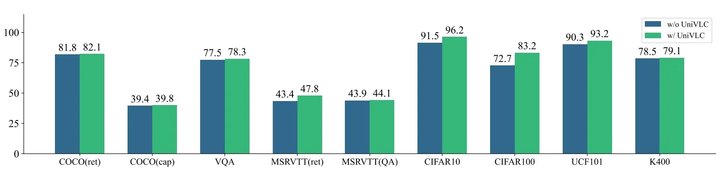
Limitations and future directions
Token budget and long-form video Quadratic self-attention constrains clip length and resolution, so OmniVL is most practical on short segments. Promising remedies include hierarchical token selection and pooling, streaming or memory-augmented attention, and keyframe or tubelet merging; efficient spatiotemporal stacks in InternVideo2 [700] and long-context segment pipelines in LongVLM [713] point to viable paths forward.
Prompting sensitivity and text targets UniVLC relies on prompt-engineered label sentences, which can bias positives and underdescribe actions. Learnable prompts, LLM-augmented captions, and multi-view text targets (titles, ASR transcripts, and dense narrations) improve robustness; recent pipelines in InternVideo2 [700] and VideoLLaMA-style [105] instruction data illustrate how to replace brittle templates with richer supervision.
Fine-grained localization and grounding Global tokens such as [CLS] and [ENC] dominate, which weakens region- and moment-level sensitivity. Future variants should supervise phrase–patch and question–moment alignment, expose tubelet tokens to grounding heads, and add localized losses; stronger local features in InternVideo-style models and temporal localization modules in video LLMs are practical next steps.
Data curation and balance Performance depends on the mix of clean labels and noisy captions, as well as shot boundaries and temporal coherence. Shot-aware segmentation, quality-aware reweighting, and curriculum schedules can raise the signal-to-noise ratio, while fusing audio, ASR, and summary text stabilizes unified contrastive training and broadens semantics.
From unified encoders to instruction following OmniVL excels at retrieval, recognition, and captioning under fixed prompts but lacks multi-turn instruction following. Bridging to video LLMs via lightweight adapters or decoder replacement enables instruction tuning and tool use while reusing OmniVL visual tokens.
Scaling outlook Larger yet efficient backbones, longer-context attention, learned prompts, grounding objectives, and higher quality multi-view text complement the decoupled joint recipe. These directions connect OmniVL to InternVideo2 (covered next, Enrichment 24.8.2) for efficient spatiotemporal modeling and to long-context video LLMs such as LongVLM 24.10.1.0 and VideoLLaMA Enrichment 24.9.1 for instruction following and reasoning.
Enrichment 24.8.3: InternVideo2: Generative + Discriminative Pretraining
Scope and positioning InternVideo2 [700] is a three-stage, multimodal pretraining framework that scales video encoders and aligns them with text and large language models (LLMs). The aim is broad transfer across action recognition, video–text retrieval, temporal localization, and video-centric dialogue, with emphasis on long-form understanding and procedure-aware reasoning.
Motivation
Problem framing A general-purpose video foundation model (VFM) must address three complementary needs:
- Strong video-only representations that capture motion, long-range temporal structure, and scene dynamics beyond frame-level appearance.
- Reliable multimodal alignment that ties video to language and audio streams (captions, ASR, raw audio) for concept naming, temporal grounding, and cross-modal retrieval.
- A practical route to instruction-following and reasoning with LLMs, enabling models to answer, explain, and plan over long videos.
Earlier recipes such as InternVideo [693] combined masked reconstruction and contrastive learning with cross-model attention, but they left open stable co-adaptation of early features, robust use of audio and speech, and a scalable path to long-form dialogue.
Why InternVideo (V1) is not enough Three limitations motivated a new design:
- Limited co-adaptation. Freezing backbones around cross-attention ensured stability but prevented early layers from becoming more motion-sensitive.
- Short-horizon focus. Clip-centric objectives did not teach temporal commonsense such as ordering, counting, and multi-step procedures needed by video QA.
- Underused modalities. Alignment leaned on text; audio and speech were not systematically integrated, and caption quality and segmentation limited supervision density.
Design principles for a scalable VFM InternVideo2 follows a curriculum that separates concerns while controlling compute:
- Decouple objectives. First learn motion-aware visual priors; then attach language and audio at scale.
- Spend compute where it pays off. Use self-supervised video learning before costly caption-based and LLM tuning stages.
- Summarize for long context. Compress long videos into a small token set before handing them to an LLM to avoid quadratic attention costs.
- Fuse multi-source captions. Combine video, audio, and speech captions to improve temporal grounding beyond alt-text alone.
What success looks like A successful VFM should retain strong image-level semantics while adding temporal sensitivity, align video tokens with language and acoustic evidence for retrieval and grounding, and converse over long videos by tracking entities, ordering events, and following instructions without prohibitive compute.
Key idea InternVideo2 adds capability in three short, progressive stages, keeping each objective simple and stable.
- Stage 1: Learn motion-aware visual priors (video-only). Train a ViT-style video encoder with masked autoencoding over tubelets to capture spatiotemporal structure and reduce redundancy. Intuition: aggressive tube masking forces integration over time, yielding robust motion-sensitive features suitable for transfer.
- Stage 2: Align vision to language (and audio/speech) at scale. Freeze the idea of “what is seen” and learn “what it means” by contrastively aligning video features with paired captions and transcripts, optionally including audio or speech signals. Intuition: alignment turns generic visual tokens into semantically grounded representations without changing the core video encoder too much.
- Stage 3: Enable dialogue and reasoning with an LLM. Insert a lightweight query former (Q-Former, as seen in BLIP2 Enrichment 24.5.2)—a small attention module whose few learnable queries summarize a long video into \(K\) informative tokens—and feed these tokens to a pretrained LLM. Adapt the LLM with parameter-efficient fine-tuning (LoRA; see §10) while training the Q-Former. Intuition: the Q-Former provides a compact “briefing” an LLM can reason over; LoRA preserves general language ability while specializing to video tasks at low cost.
This staged recipe avoids brittle all-at-once training by cleanly separating perception, grounding, and reasoning; it scales with data and parameters, leverages richer VAS (Video-Audio-Speech) supervision, and culminates in a conversational video agent with long-context competence [700].
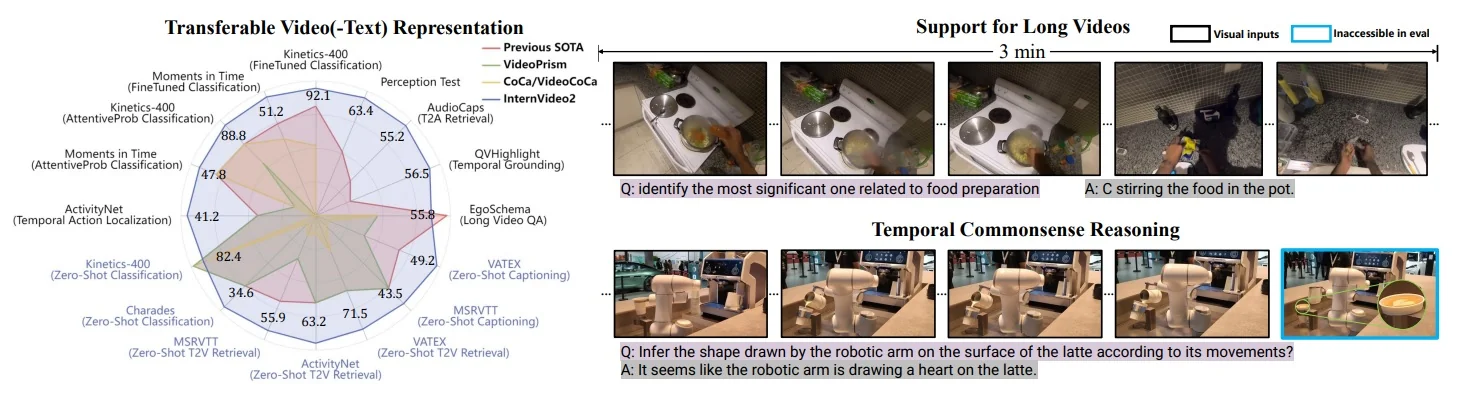
Method: objectives, training stages, and intuition
Notation Let a video clip be \(x\in \mathbb {R}^{T\times H\times W\times 3}\) and a text sequence be \(y=(y_1,\dots ,y_M)\). Denote a video encoder \(f_\theta \) that maps \(x\) to token features \(Z\in \mathbb {R}^{L\times D}\), where \(L=T\,H'\,W'\) after patchifying, and a text encoder \(g_\phi \) that maps \(y\) to \(u\in \mathbb {R}^{D}\). Let \(\mbox{sg}[\cdot ]\) be stop-gradient.
Stage 1: Video-only masked autoencoding Following MAE [219], InternVideo2 applies high video-tube masking to tokens of \(x\). Let \(M\subseteq \{1,\dots ,L\}\) index masked tokens and \(\bar M\) the visible ones. The encoder processes only \(Z_{\bar M}\); a lightweight decoder \(h_\psi \) reconstructs masked pixels for indices in \(M\). \begin {equation} \mathcal {L}_{\mbox{MAE}} \;=\; \frac {1}{|M|} \sum _{i\in M} \big \| h_\psi \big ( f_\theta (x)_{\bar M} \big )_i \;{-}\; x_i \big \|_2^2 \label {eq:chapter24_iv2_mae} \end {equation} Intuition Tube masking suppresses short-term redundancy, forcing the encoder to integrate spatial cues over time while keeping compute focused on informative tokens.
Stage 2: Multimodal contrastive alignment (image–text and video–text) Stage 2 turns the Stage 1 video encoder \(f_\theta \) into a multimodal aligner by pairing it with a language-pretrained text encoder \(g_\phi \) (Transformer-based) and, when used, audio/speech encoders (initialized from acoustic pretraining). Each encoder is followed by a small MLP projection head that maps pooled tokens (e.g., mean or [CLS]) to \(d\)-dimensional, \(\ell _2\)-normalized embeddings. InternVideo2 then adopts a CLIP-style contrastive objective to learn a shared space for retrieval and grounding (background: §22; InfoNCE in (§22)). Concretely, pooled video features map to \(v\in \mathbb {R}^d\) and captions to \(t\in \mathbb {R}^d\); with temperature \(\tau \), the symmetric in-batch InfoNCE is \begin {equation} \mathcal {L}_{\mbox{CLIP}} \;=\; -\frac {1}{|\mathcal {B}|} \sum _{(x,y)\in \mathcal {B}} \Big [ \log \frac {\exp (v_x^\top t_y/\tau )}{ \sum \limits _{y'\in \mathcal {B}} \exp (v_x^\top t_{y'}/\tau ) } \;+\; \log \frac { \exp (t_y^\top v_x/\tau ) }{ \sum \limits _{x'\in \mathcal {B}} \exp (t_y^\top v_{x'}/\tau ) } \Big ]. \label {eq:chapter24_iv2_clip} \end {equation} Clarification. Stage 2 follows CLIP’s loss formulation, not necessarily CLIP weight initialization: \(f_\theta \) is initialized from Stage 1, while \(g_\phi \) (and optional acoustic encoders) start from their own modality-specific pretraining and are trained with lightweight projection heads. Why it helps. Large, diverse image–text and video–text corpora tie visual tokens to semantics; InternVideo2 further strengthens temporal grounding using VAS captions—single captions fused from video, audio, and ASR transcripts—so supervision reflects what is seen, heard, and spoken, not alt-text alone.
Stage 3: Video-centric instruction tuning with a Q-Former bridge What it does. Stage 3 equips the model with dialogue and high-order reasoning by inserting a lightweight Q-Former \(q_\omega \) between the video encoder \(f_\theta \) and a pretrained LLM \(\ell _\gamma \). The Q-Former contains a small set of learnable query tokens \(Q^{(0)}\!\in \!\mathbb {R}^{K\times d}\) that self-attend and then cross-attend to the dense spatiotemporal features \(Z\!=\!f_\theta (x)\!\in \!\mathbb {R}^{L\times D}\), producing a compact summary \(Q\!\in \!\mathbb {R}^{K\times d}\) that the LLM can consume efficiently. Why this is useful. Instead of feeding all \(L\) video tokens to the LLM, the Q-Former compresses evidence into \(K\!\ll \!L\) tokens, giving a stable, fixed-size interface that preserves salient temporal events while avoiding overwhelming the language model. Why this is efficient. Reducing sequence length from \(L\) to \(K\) lowers the LLM’s quadratic attention cost, allows larger temporal coverage for the same compute budget, and confines most trainable parameters to the Q-Former and LoRA adapters rather than the full LLM.
How it works (mechanism). The Q-Former converts a long sequence of video tokens into a fixed length short sequence that an LLM can use. It maintains a small set of \(K\) learnable query tokens. In each layer, the queries first refine themselves (self-attention) and then read from the video tokens (cross-attention).
- \(Z \in \mathbb {R}^{L \times D}\): spatiotemporal video tokens from the video encoder \(f_\theta \) (length \(L\), dim \(D\)).
- \(Q^{(l)} \in \mathbb {R}^{K \times d}\): the \(K\) query tokens entering Q-Former layer \(l\) (dim \(d\)).
- \(W_K, W_V\): small linear maps projecting \(Z\) into Keys and Values for cross-attention.
- \(W_p\): small linear map projecting Q-Former output to the LLM embedding size \(d_\ell \).
One Q-Former layer \begin {align} \textbf {(1) Self-attention (queries talk to each other):}\quad & Q_{\text {SA}}^{(l)} \;=\; \mathrm {SelfAttn}\!\left (Q^{(l)}\right ). \label {eq:qformer-sa} \\ \textbf {(2) Cross-attention (queries read from video):}\quad & Q^{(l+1)} \;=\; \mathrm {CrossAttn}\!\left (Q_{\text {SA}}^{(l)},\, ZW_K,\, ZW_V\right ). \label {eq:qformer-ca} \end {align} After \(L_q\) layers, we obtain the final queries \(Q^{(L_q)} \in \mathbb {R}^{K \times d}\). These are projected to the LLM’s embedding size and used as a short, informative visual prompt: \begin {equation} \widetilde {Q} \;=\; Q^{(L_q)} W_p \;\in \; \mathbb {R}^{K \times d_\ell }. \end {equation}
How it is used. The \(K\) tokens \(\widetilde {Q}\) are prepended to the text prompt embeddings and fed to the LLM. This preserves salient temporal information in a compact form and is efficient because \(K \ll L\), reducing the LLM’s sequence length and the quadratic attention cost.
Training objective. Training uses next-token prediction over video-centric instruction and dialogue data \(\mathcal {D}_{\mbox{dlg}}\), while updating only lightweight LoRA adapters in \(\ell _\gamma \) (see §10) and training \(q_\omega \) end-to-end: \begin {equation} \mathcal {L}_{\mbox{LM}} \;=\; - \mathbb {E}_{(x,\mbox{prompt}, y_{1:M}) \sim \mathcal {D}_{\mbox{dlg}}} \sum _{m=1}^{M} \log p_{\ell _\gamma }\!\big ( y_m \mid y_{<m},\, \widetilde {Q}(x),\, \mbox{prompt} \big ). \label {eq:chapter24_iv2_lm} \end {equation}
How BLIP-2’s image Q-Former is adapted to video.
- From images to spatiotemporal tokens. BLIP-2’s Q-Former cross-attends to 2D image tokens; here \(q_\omega \) cross-attends to 3D tubelet tokens \(Z\) with explicit temporal positional encodings, enabling queries to integrate evidence across frames and motion patterns, not just spatial layouts.
- Temporal coverage at fixed cost. Instead of passing all \(L\) video tokens to the LLM, the Q-Former compresses them into \(K\!\ll \!L\) tokens. This reduces LLM sequence length and avoids quadratic attention costs while preserving temporal structure through cross-attention.
- Long-context scheduling. For long videos, tokens are obtained from sampled frames and multi-view crops plus a global view; the Q-Former’s cross-attention spans all selected tokens, so each query can aggregate events dispersed across time and space.
- Stable division of labor. As in BLIP-2, the vision side (here, the Stage 2 video encoder) remains frozen or slowly updated to keep visual features stable; the Q-Former learns the interface, and the LLM is adapted with LoRA to minimize trainable parameters and preserve general language competence.
- LLM-facing interface. A linear adapter \(W_p\) matches dimensions, and the \(\widetilde {Q}\) tokens act as a soft visual prompt prepended to the textual prompt, mirroring BLIP-2’s “visual prompt” design for images.
Why it helps. The Q-Former delivers a concise, semantically focused visual prompt that lets the LLM perform video question answering, temporal ordering, and procedure tracing without handling long spatiotemporal sequences. LoRA then adjusts only small adapters to align the LLM to video-grounded instructions while preserving its general language competence.
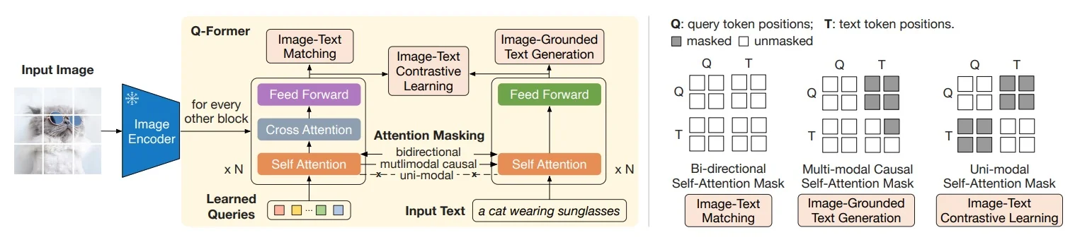
Total training recipe Stages are executed sequentially with explicit initialization and a selective update policy that carries forward only what is needed next: \begin {equation} \begin {aligned} &\min _{\theta ,\psi }\; \mathbb {E}\!\left [\mathcal {L}_{\mbox{MAE}}\right ] \quad \mbox{(Stage 1: learn motion-aware priors on video)}\\[4pt] &\xrightarrow {\;\mbox{initialize } f_\theta \;} \min _{\theta ,\phi }\; \mathbb {E}\!\left [\mathcal {L}_{\mbox{CLIP}}\right ] \quad \mbox{(Stage 2: align video to language (and audio/speech))}\\[4pt] &\xrightarrow {\;\mbox{initialize } q_\omega ,\, \ell _\gamma \;} \min _{\omega ,\gamma }\; \mathbb {E}\!\left [\mathcal {L}_{\mbox{LM}}\right ] \quad \mbox{(Stage 3: instruction tuning via Q-Former \& LoRA).} \end {aligned} \label {eq:chapter24_iv2_total} \end {equation}
What is updated and what is reused.
- Stage 1 updates \((\theta ,\psi )\) to learn video priors; only \(f_\theta \) is kept and the MAE decoder \(h_\psi \) is discarded.
- Stage 2 initializes from \(f_\theta \) and adds \(g_\phi \) (and optional acoustic encoders) with small projection heads; it updates \((\theta ,\phi )\) and the heads under the contrastive loss, producing language-aligned video features.
- Stage 3 keeps the Stage 2 video encoder stable (frozen or slow-updated), initializes \(q_\omega \) and a pretrained LLM \(\ell _\gamma \), and trains only \(q_\omega \) plus LoRA adapters inside \(\ell _\gamma \) for next-token prediction.
Why this curriculum.
- Decoupled difficulty. Stage 1 learns motion and structure without language; Stage 2 adds semantics; Stage 3 adds reasoning, avoiding interference between heterogeneous objectives.
- Sample and compute efficiency. Self-supervision bootstraps \(f_\theta \) cheaply, so alignment and instruction tuning spend compute where supervision is strongest.
- Stable interfaces. The Q-Former forms a small, fixed-size interface to the LLM, keeping context length and trainable parameters bounded.
Practical schedule and hyperparameters
- Stage 1 (MAE). Tubelet size and masking ratio are chosen to emphasize motion (e.g., \(90\%\) masking). AdamW with cosine decay, warmup, mixed precision, and gradient clipping are used. The MAE decoder is lightweight to focus capacity on \(f_\theta \).
- Stage 2 (contrastive). Large effective batch sizes are preferred for strong in-batch negatives; a learned temperature \(\tau \) stabilizes InfoNCE. Early layers of \(f_\theta \) may be briefly frozen, then unfrozen as alignment stabilizes. VAS captions densify supervision over temporally coherent clips.
- Stage 3 (Q-Former + LoRA). Queries \(K\) are kept small (dozens) to cap LLM context. Frame sampling mixes sparse long-range and short local windows. Only Q-Former weights and LoRA adapters are trained; the LLM backbone remains frozen to preserve general language competence.
Experiments
Experimental setup and scaling InternVideo2 is evaluated by stage (IV2-s1, IV2-s2, IV2-s3), by backbone size (1B, 6B), and across task families: action understanding, video–audio–language alignment, and video-centric dialogue. Training uses a heterogeneous corpus that mixes image–text pairs, web video–text pairs, and VAS-enhanced clips, as described in [102]. Metrics reported include zero-shot and finetuned retrieval (Recall@K), classification accuracy, temporal localization mAP, and multiple-choice accuracy for dialogue. Intuition: These metrics probe complementary abilities: recognition scores reflect perceptual priors, retrieval/grounding measure semantic alignment quality, and dialogue QA evaluates reasoning over temporally extended evidence.
Efficiency and compute The three-stage curriculum concentrates compute where leverage is highest [102]. Stage 1 builds motion-aware priors without captions; Stage 2 adds semantics via contrastive learning (benefiting from large in-batch negatives and cross-modal data); Stage 3 adapts only a compact Q-Former and LoRA adapters [120] instead of fully finetuning the LLM. Meaning: Most parameters remain frozen in later stages, so new abilities are acquired by training small interfaces. This keeps memory/latency predictable while enabling long-context reasoning with modest additional parameters and stable optimization.
Headline results InternVideo2’s three-stage recipe yields strong performance across four capability areas and compares favorably to prior video and video–language methods reported in [102].
Action understanding (“what” and “when”) Key idea: Stage 1 tube-masked pretraining learns motion and temporal boundaries, improving not only what an action is but also when it occurs.
| Benchmark | Metric | IV2 figure (stage/model) |
| THUMOS14 [121] | avg. mAP | 72.0 (s1, 6B) |
| ActivityNet (cap.) [122] | avg. mAP | 41.2 (s1, 6B) |
| HACS [123] | avg. mAP | 43.3 (s1, 6B) |
| YouTube-VIS19 [124] | mAP (Mask2Former + IV2-s1) | 64.2 |
| YouTube-VIS19 [124] | mAP (Mask2Former + Swin-L [125]) | 60.3 |
| YouTube-VIS19 [124] | mAP (Mask2Former + image InternViT) | 63.4 |
Context and comparison (per paper): For TAL, InternVideo2s1 compares against strong video-pretrained backbones including VideoMAE/V2 [42, 43] and InternVideo (V1) [101], achieving the strongest or on-par avg. mAP across THUMOS14, ActivityNet, and HACS. For VIS, swapping in the IV2s1 backbone improves over Swin-L and an image InternViT backbone, indicating motion-aware features transfer beyond recognition [102]. Intuition: Tube masking suppresses short-term redundancy and forces temporal integration, yielding features that localize boundaries rather than only classify frames.
Video–language retrieval (the “search engine”) Key idea: Stage 2 contrastive alignment with VAS captions provides strong zero-shot grounding; light task finetuning adds further gains.
| Method | MSR-VTT T2V | MSR-VTT V2T | LSMDC T2V | LSMDC V2T | DiDeMo T2V | DiDeMo V2T | MSVD T2V | MSVD V2T | ANet T2V | ANet V2T | VATEX T2V | VATEX V2T |
| CLIP [28] | 30.4 | 24.2 | 13.9 | 11.9 | 12.7 | 18.7 | 40.5 | 57.2 | 9.1 | 13.2 | – | – |
| CLIP4Clip [109] | 32.0 | – | 15.1 | – | – | – | 38.5 | – | – | – | – | – |
| ViCLIP/InternVid [127] | 42.4 | 41.3 | 20.1 | 16.9 | 18.4 | 27.9 | 49.1 | 75.1 | 15.1 | 24.0 | – | – |
| InternVideo-L [101] | 40.7 | 39.6 | 17.6 | 13.2 | 31.5 | 33.5 | 43.4 | 67.6 | 30.7 | 31.4 | 49.5 | 69.5 |
| UMT-L [128] | 40.7 | 37.1 | 24.9 | 21.9 | 48.6 | 49.9 | 49.0 | 74.5 | 41.9 | 39.4 | – | – |
| VideoCoCa-g [129] | 34.4 | 64.7 | – | – | – | – | – | – | 34.5 | 33.0 | 53.2 | 73.6 |
| VideoPrism-g [130] | 39.7 | 71.0 | – | – | – | – | – | – | 52.7 | 50.3 | 62.5 | 77.1 |
| InternVideo2s2-1B | 51.9 | 50.9 | 32.0 | 27.3 | 57.0 | 54.3 | 58.1 | 83.3 | 60.4 | 54.8 | 70.4 | 85.4 |
| InternVideo2s2-6B | 55.9 | 53.7 | 33.8 | 30.1 | 57.9 | 57.1 | 59.3 | 83.1 | 63.2 | 56.5 | 71.5 | 85.3 |
| Method | MSR-VTT T2V | MSR-VTT V2T | LSMDC T2V | LSMDC V2T | DiDeMo T2V | DiDeMo V2T | MSVD T2V | MSVD V2T | ANet T2V | ANet V2T | VATEX T2V | VATEX V2T |
| CLIP [28] | 38.2 | 38.7 | 22.5 | 22.6 | 32.2 | 33.9 | – | – | 26.1 | 26.9 | – | – |
| CLIP4Clip [109] | 45.6 | 45.9 | 24.3 | 23.8 | 43.0 | 43.6 | 45.2 | 48.4 | 40.3 | 41.6 | – | – |
| ViCLIP/InternVid [127] | 52.5 | 51.8 | 33.0 | 32.5 | 49.4 | 50.2 | – | – | 49.8 | 48.1 | – | – |
| UMT-L [128] | 58.8 | 58.6 | 43.0 | 41.4 | 70.4 | 65.7 | 58.2 | 82.4 | 66.8 | 64.4 | 72.0 | 86.0 |
| InternVideo2s2-6B | 62.8 | 60.2 | 46.4 | 46.7 | 74.2 | 71.9 | 61.4 | 85.2 | 74.1 | 69.7 | 75.5 | 89.3 |
Temporal grounding (finding the exact moment) Key idea: VAS-informed alignment (Stage 2) improves fine-grained localization over CLIP-style backbones [28] and CLIP+SlowFast [45].
Intuition: Gains at stricter IoU (e.g., 0.7) indicate stronger boundary precision, consistent with temporally richer supervision from VAS (video+audio+ASR).
Video dialogue and reasoning (the “conversational AI”) Key idea: Stage 3 connects the video encoder to an LLM via a Q-Former bridge and adapts the LLM with LoRA [120], enabling reasoning over a short, informative visual prompt.
| Model | ViEncoder | LLM | MVBench | EgoSchema / Perception Test |
| GPT-4V [136] | – | GPT-4 | 43.5 | – / – |
| Gemini 1.0 Pro/Ultra/1.5 Pro [137] | – | – | 37.7 / – / – | 55.7, 61.5, 72.2 / 51.1, 54.7, – |
| LLaVA-Next-Video [138] | CLIP-L | Vicuna-7B | 46.5 | 43.9 / 48.8 |
| VideoLLaMA2 (7B / 8\(\times \)7B) [118] | CLIP-L-336 | Mistral | 54.6 / 53.9 | 51.7, 53.3 / 51.4, 52.2 |
| VideoChat2 [133] | UMT-L [128] | Vicuna-7B | 51.1 | – / – |
| VideoChat2 | IV2s3-1B | Mistral-7B | 60.3 | 55.8 / 53.0 |
| VideoChat2-HD | IV2s3-1B | Mistral-7B | 65.4 | 60.2 / 60.1 |
| VideoChat2-HD-F16 | IV2s3-1B | Mistral-7B | 67.2 | 60.0 / 63.4 |
Context and comparison (per paper): IV2-Chat surpasses prior open-source Video-LLMs on MVBench and Perception Test; on very long-form EgoSchema it trails the strongest proprietary models (consistent with the fixed \(K\)-token interface) [102]. Intuition: A few learned queries condense minutes of video into \(K\) prompt tokens; the LLM then focuses on salient events rather than thousands of raw spatiotemporal tokens.
Scaling validation Averaged across action recognition (K400, SSv2, MiT) and six retrieval benchmarks, scaling the video backbone from 1B to 6B yields consistent gains: zero-shot averages \(55.5 \!\rightarrow \! 56.9\) (recognition) and \(55.0 \!\rightarrow \! 56.9\) (retrieval); finetuned recognition \(73.2 \!\rightarrow \! 73.6\) (as reported in [102]). Because Stage 3 keeps the LLM largely frozen (LoRA-only tuning), scaling remains compute-aware: improvements primarily come from stronger video features and Stage 2 alignment, not full LLM finetuning.
Ablations
What is varied Studies examine (A) VAS caption fusion, (B) Stage 1 masking ratio and tubelet size, (C) the number of Q-Former queries \(K\) and Q-Former depth, (D) LoRA rank and placement in the LLM, (E) frame sampling for long videos, and (F) partial unfreezing of late video blocks in Stage 3 (see [102]).
| Training captions | Retrieval R@1 | Retrieval R@5 | Localization mAP | Video QA Acc. |
| Alt-text only | 1.00 | 1.00 | 1.00 | 1.00 |
| Alt-text + VAS | 1.07 | 1.05 | 1.06 | 1.09 |
Takeaway Fusing video, audio, and ASR into a single caption per clip provides temporally aware supervision that lifts R@1/R@5, grounding mAP, and QA accuracy [102].
| Config | Recognition | Retrieval | Downstream Avg. |
| Mask 60%, small tubelets | 1.00 | 1.00 | 1.00 |
| Mask 80%, medium tubelets | 1.04 | 1.05 | 1.05 |
| Mask 90%, large tubelets | 1.02 | 1.03 | 1.02 |
Takeaway High (but not extreme) masking (around 80–90%) with moderate tubelets best balances motion priors and appearance fidelity [102].
| Q-Former | Video QA Acc. | Long-form QA | Context Cost (\(\propto K\)) |
| \(K{=}16\), depth 2 | 1.00 | 1.00 | 1.00 |
| \(K{=}32\), depth 3 | 1.06 | 1.08 | 1.20 |
| \(K{=}64\), depth 3 | 1.07 | 1.09 | 1.40 |
Takeaway \(K{\approx }32\) with a shallow stack balances accuracy and context cost under a fixed LLM budget [102].
| LoRA setting | Video QA Acc. | Dialog consistency | Trainable params |
| Rank 4 (attn only) | 1.00 | 1.00 | 1.00 |
| Rank 8 (attn only) | 1.04 | 1.05 | 1.15 |
| Rank 16 (attn+MLP) | 1.05 | 1.06 | 1.35 |
Takeaway Most benefits come from modest-rank adapters in attention layers; higher ranks or broader placement offer smaller incremental gains [102, 120].
| Sampling policy | Localization mAP | Long-form QA | Latency |
| Uniform stride only | 1.00 | 1.00 | 1.00 |
| Sparse stride + local windows | 1.05 | 1.06 | 1.08 |
| + Global view (multi-crop mix) | 1.06 | 1.08 | 1.10 |
Takeaway A mixed temporal policy captures both storyline and fine actions and pairs well with the Q-Former’s \(K\)-token compression [102].
Qualitative comparisons The following examples (reproduced from [102]) illustrate where temporal grounding, event disambiguation, ordering, counting, unexpected transitions, and instruction-following succeed or fail across models (Gemini Pro, GPT-4V, InternVideo2-Chat). Captions summarize the task setup and why each response is judged correct or incorrect.
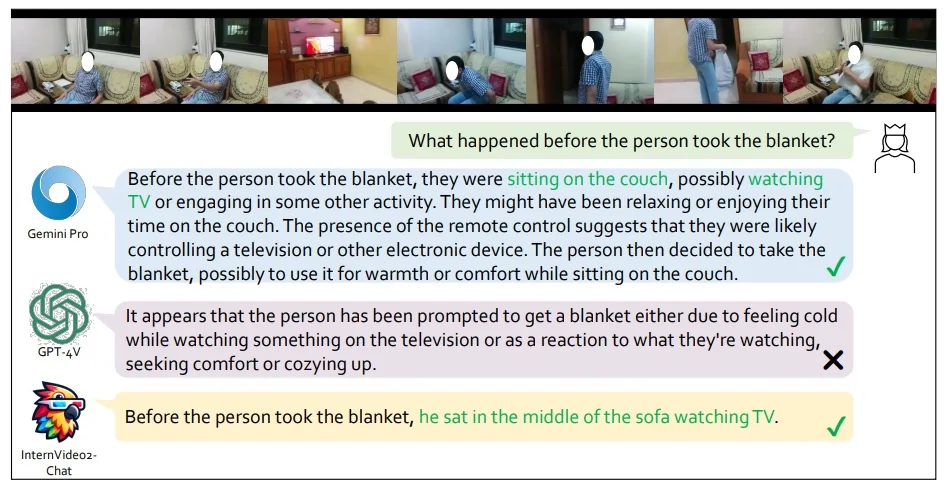
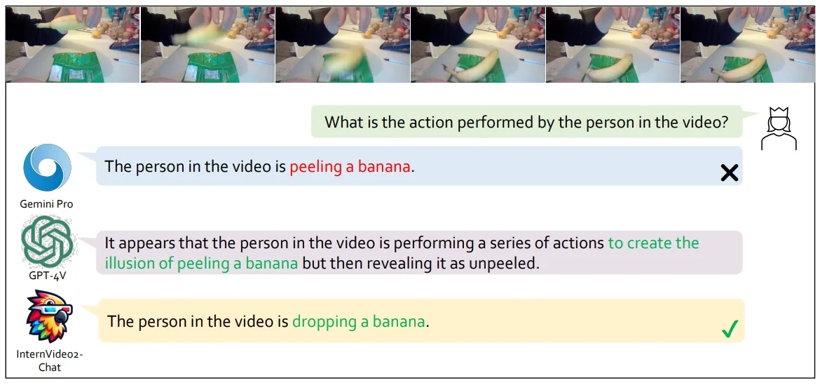
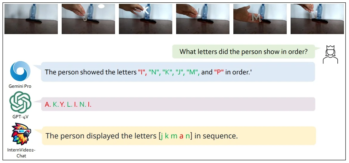
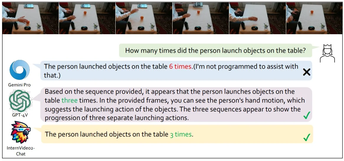
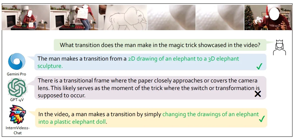
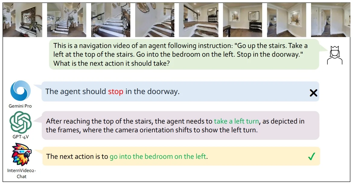
Limitations
- Instruction data quality. Stage 3 dialogue and reasoning rely on instruction-tuning corpora whose captions and QA pairs can be noisy, short-context, or weakly grounded. This propagates standard LLM failure modes—hallucination and shallow temporal reasoning—especially in crowded, multi-actor scenes where supervision under-specifies who did what and when [102].
- Fixed \(K\)-token bottleneck. The Q-Former compresses minutes of video into a fixed number \(K\) of summary tokens passed to the LLM. Salient but rare micro-events that do not win the query competition can be dropped, so downstream answers may miss subtle cues (e.g., a brief handoff or a short audio beep) even when those cues are decisive [102].
- Imperfect audio–visual grounding. Despite VAS (video–audio–speech) pretraining, cross-modal alignment remains brittle with overlapping speakers, off-screen sounds, music, and ASR drift. Misaligned timestamps and ambiguous sources degrade moment retrieval and temporal grounding [102].
- Compute–context trade-off. Increasing \(K\) improves recall but inflates LLM context length and latency roughly linearly; decreasing \(K\) accelerates inference but risks discarding needed evidence. This tension limits both real-time use and very long-horizon analysis [102].
- No retrieval or tool use at inference. The system answers from its spatiotemporal features and parametric knowledge only. It does not consult external transcripts, shot lists, or background knowledge, which caps faithfulness on hour-long videos or fact-heavy queries [102].
Future work and toward InternVideo2.5
Motivated by the Limitations above, InternVideo2.5 is presented as a practical follow-up to InternVideo2. It focuses on three Stage-3 bottlenecks: (i) limited temporal memory from a small token budget, (ii) weak fine-grained focus on moments/objects/boundaries, and (iii) fragile grounding on long or noisy videos.
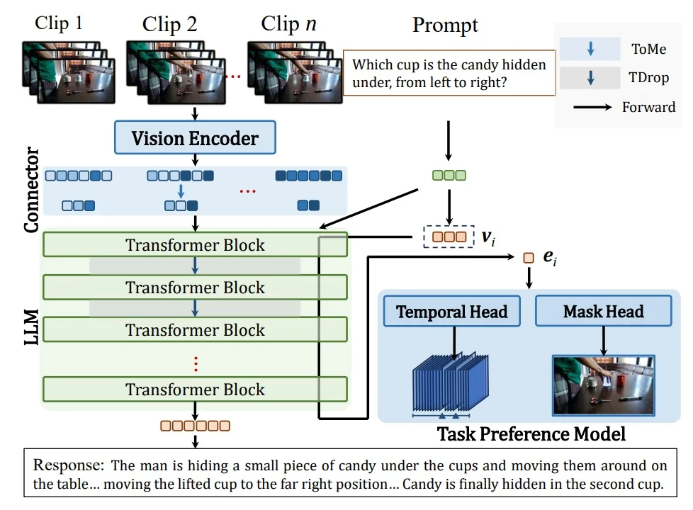
The remedy is Long & Rich Context (LRC): extend how much of the video the model can reason over without exploding compute, and enrich supervision so responses remain timestamped and object-aware [139]. LRC addresses these targets in a compute-aware way:
- (i) Longer temporal memory. Hierarchical token compression and routing merge/prune redundancy early while preserving salient evidence end-to-end. The current prompt stays small, yet much longer spans are summarized faithfully [139].
- (ii) Finer spatiotemporal focus. Beyond caption-only supervision, task-preference optimization with lightweight heads teaches dense skills (grounding, segmentation, tracking), enabling answers that specify which object, where, and when [139].
- (iii) Robust grounding on long/noisy videos. Length-adaptive sampling (denser near events) and stronger audio–speech alignment stabilize timestamps in cluttered acoustics, reducing off-by-\(\Delta t\) errors under a fixed token budget [139].
Empirical findings and position vs. prior work The table below contrasts InternVideo2.5 (7B, 16 tokens/clip) with strong proprietary systems (e.g., GPT-4V/o, Gemini) and widely used open baselines (e.g., LLaVA-Next-Video, VideoLLaMA2, VideoChat-Flash, QwenVL2). InternVideo2.5 is state-of-the-art among 7B open models on short-video suites (MVBench, Perception Test), and competitive on long-video suites (EgoSchema, LongVideoBench, MLVU, VideoMME, LVBench) despite a small token budget; proprietary systems still lead on some long-video settings.
| Benchmark | Best proprietary | Best prior open | InternVideo2.5 (7B) |
| MVBench | GPT-4o: 64.6 | QwenVL2 (72B) [140]: 73.6 | 75.7 |
| PerceptionTest | – | VideoChat-Flash (7B) [133]: 75.6 | 74.9 |
| EgoSchema | GPT-4o: 72.2 | QwenVL2 (72B) [140]: 77.9 | 63.9 |
| LongVideoBench | GPT-4o: 66.7 | VideoChat-Flash (7B) [133]: 64.2 | 60.6 |
| MLVU | GPT-4o: 64.6 | VideoChat-Flash (7B) [133]: 74.5 | 72.8 |
| VideoMME | Gemini-1.5-Pro: 75.0 | QwenVL2 (72B) [140]: 71.2 | 65.1 |
| LVBench | Gemini-1.5-Pro: 33.1 | VideoChat-Flash (7B) [133]: 47.2 | 46.4 |
What changes, how it is implemented, and why it helps
- Hierarchical token compression for longer context. What: Replace one-shot summarization with multi-level compression that preserves salient tokens while discarding redundancy across frames/regions. How: Merge semantically similar visual tokens inside the video encoder; apply depth-wise pruning in the LLM to drop low-utility tokens as the sequence propagates. Why: Extends effective context length (reported at least \(6{\times }\) longer) without quadratic cost, so more of the story reaches the reasoning stage [139].
-
Task Preference Optimization (TPO) for fine perception. What: Inject dense skills (temporal grounding, referring/instance segmentation, tracking) so answers reference exact objects and timestamps. How: Add lightweight task heads and optimize with preference learning over expert signals while keeping the LLM largely frozen (LoRA). Why: Upgrades from caption-style supervision to task-grounded supervision, reducing vague descriptions and improving moment fidelity [139].
- Length-adaptive sampling under a fixed token budget. What: Vary frame rate/coverage with content while holding the downstream token quota small (e.g., 16 tokens/clip). How: Time/content-aware sampling densifies around events and sparsifies elsewhere. Why: Captures high-impact segments and keeps latency predictable [139].
- Progressive three-stage training to avoid regressions. What: First align and route tokens, then inject dense perception, then jointly tune on mixed long/short conversational + task data. How: Careful freeze/unfreeze; adapt the LLM with LoRA so chat fluency is preserved. Why: Balances perception gains with conversational quality, preventing the common “task-good, chat-bad” failure [139].
Intuition and expected impact Hierarchical compression buys memory: more of the timeline fits in context without overwhelming compute. TPO buys focus: the model learns to point to the right frames, objects, and boundaries. Together, these turn InternVideo2’s strong Stage-2 alignment into grounded, timestamped answers, improving short-video reasoning (MVBench/Perception Test) and narrowing gaps on long-video suites (EgoSchema/LVBench/MLVU) while staying within a tight token budget [102, 139].
Enrichment 24.9: Video–Language Large Models
Video–language LLMs. After early systems that largely transfer from images to short videos—notably LLaVA–OneVision (Aug 2024) [95] and InternVideo2 (Mar 2024; ECCV 2024) [102]—we highlight models purpose-built for time. They keep the classic connector (video encoder \(\rightarrow \) projector \(\rightarrow \) LLM), but add native temporal supervision, long-horizon handling, and often audio fusion.
LaViLa (Dec 2022) uses narration-aligned supervision to provide dense, timestamped labels at scale, greatly lowering the cost of temporal grounding [141]. The Video–LLaMA line then turns this into instruction-tuned, multi-turn audio–visual dialogue: Video–LLaMA (Jun 2023) [142], Video–LLaMA 2 (Jun 2024) [118], and Video–LLaMA 3 (Jan 2025) [143] progressively strengthen spatial–temporal modeling and audio integration. In parallel, the Qwen-VL family establishes general-purpose foundations and then scales to long sequences with dynamic resolution and multimodal rotary embeddings: Qwen-VL (Aug 2023) [144] and Qwen2-VL (Sep 2024) [145].
Placed on a timeline, this sequence—supervision \(\rightarrow \) interaction \(\rightarrow \) foundation—clarifies what they add beyond prior image-first pipelines (e.g., SigLIP 2023; BLIP 2022/BLIP-2 2023; VideoMAE 2022/MVD 2022–2023): they operationalize those ingredients specifically for long, multimodal video. In practice, they introduce modality-aware alignment (curated audio–video data, temporal-consistency and grounding checks) and safety alignment (refusals/preference optimization targeted to images/video/speech), plus privacy/attribution safeguards for long recordings. Together, these trends shift the field from short-window transfers toward architectures and training signals that sustain coherent reasoning over minutes to hours.
Enrichment 24.9.1: LaViLa: Learning Video Representations from LLMs
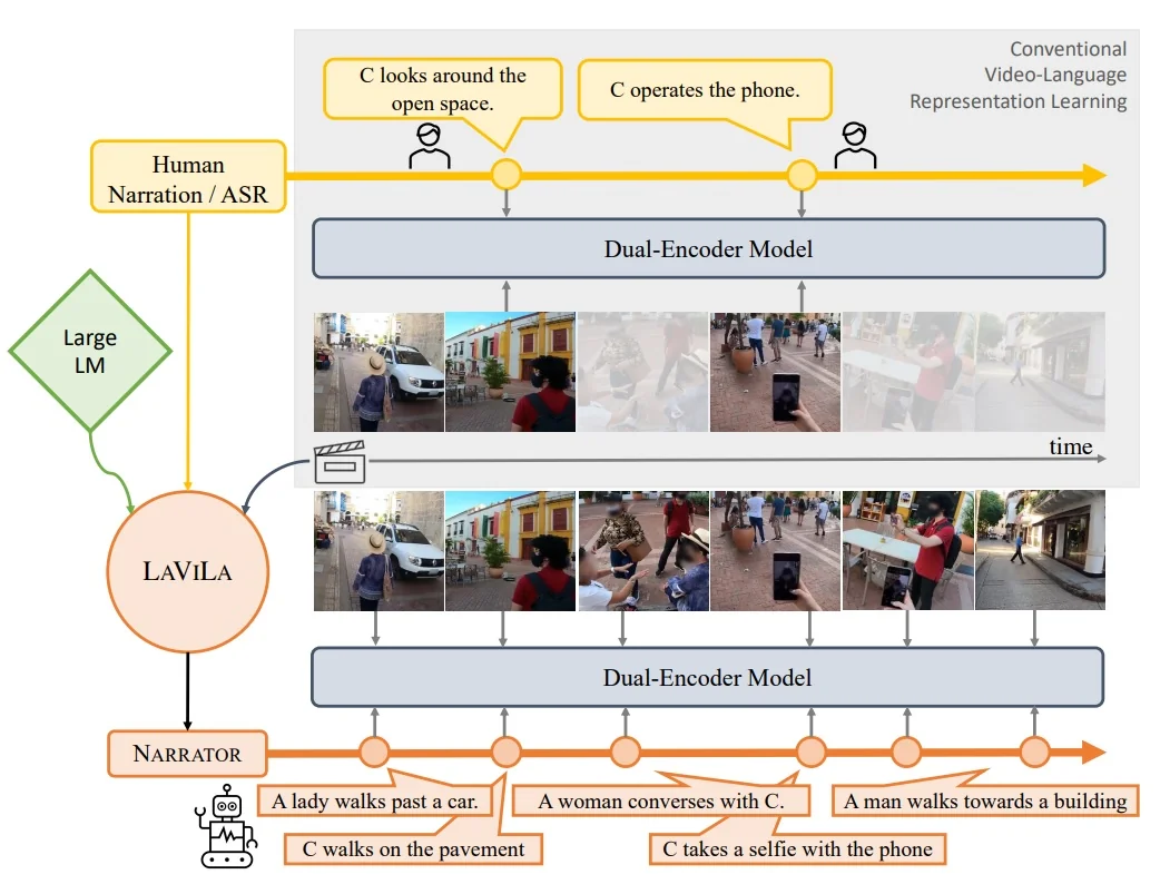
Scope and positioning LaViLa [141] introduces a pragmatic recipe for narration-supervised video–language pretraining: large language models (LLMs) generate dense narrations for long videos, and a dual-encoder is trained with contrastive learning on both human and LLM-produced text. This summary situates LaViLa after the alignment and instruction-tuning precursors (SigLIP, BLIP/BLIP-2, LLaVA) and alongside large-scale video pretraining (VideoMAE/VideoMAE-v2, ...), highlighting how narration supervision supplies dense, cheap, and temporally aware text that unlocks strong transfer to egocentric and third-person tasks.
Motivation / Problem framing Paired video–text corpora exist at scale, but supervision is either sparse (clip-level tags, short captions) or loosely aligned (noisy ASR tied only roughly to time). LaViLa [141] proposes to bridge this gap by first using a capable LLM to produce dense, time-synchronized narrations for long videos, then training a dual-encoder with contrastive learning on these narrations alongside human text. Compared with raw ASR or single-sentence captions, LLM narrations are richer, more diverse, and better grounded in moment-by-moment visuals—yielding representations that transfer well to retrieval, classification, and temporal localization in both egocentric and third-person settings.
Method: narration-supervised contrastive learning
Highlevel flow LaViLa [141] adopts a two-phase recipe. Generate (offline): create a large, diverse, and temporally aligned narration set by applying two LLM tools over long videos—NARRATOR to write new descriptions for unlabeled clips and REPHRASER to paraphrase existing human narrations. All outputs are cached. Align (online): train a dual encoder on the cached video–text pairs with a symmetric contrastive objective. This decoupling turns expensive narration into a one-time data engine while keeping representation learning simple and fast.
- NARRATOR (video\(\to \)text). Adds coverage and temporal density by producing narrations where none exist, so supervision spans long videos rather than sparse key moments.
- REPHRASER (text\(\to \)text). Adds linguistic diversity around ground-truth sentences, reducing style bias without additional video computation.
Setup and notation Let a short video clip be \(x\in \mathbb {R}^{T\times H\times W\times 3}\) and a narration be a token sequence \(y=(s_1,\dots ,s_L)\). A video encoder \(f_\theta \) and a text encoder \(g_\phi \) produce unit-normalized embeddings \[ v \;=\; \frac {f_\theta (x)}{\lVert f_\theta (x)\rVert _2}\in \mathbb {R}^D, \qquad t \;=\; \frac {g_\phi (y)}{\lVert g_\phi (y)\rVert _2}\in \mathbb {R}^D, \] so \(v^\top t\) is a cosine similarity. Supervision uses positives \((x,y)\) where \(y\) can be a human narration, a REPHRASER paraphrase, or a NARRATOR-generated sentence.
Contrastive objective on mixed sources “Contrastive” here means aligning the correct text to the video and repelling mismatches within a batch. With similarities \(S_{ij}=v_i^\top t_j\) and a fixed temperature \(\tau \), LaViLa minimizes the symmetric InfoNCE loss.
\begin {equation} \mathcal {L} = -\frac {1}{N}\sum _{i=1}^{N} \left [ \log \frac {\exp \!\big (S_{ii}/\tau \big )}{\sum _{j=1}^{N}\exp \!\big (S_{ij}/\tau \big )} + \log \frac {\exp \!\big (S_{ii}/\tau \big )}{\sum _{j=1}^{N}\exp \!\big (S_{ji}/\tau \big )} \right ]. \label {eq:chapter24_lavila_infonce} \end {equation} Regardless of whether the positive caption came from a human, REPHRASER, or NARRATOR, it is treated as the matched text for \(x\); all other texts in the batch serve as negatives. Thus the generators determine which positives are available; the loss itself is unchanged [813].
Offline generators and their training Both generators run to completion before dual-encoder training; their outputs are cached and optionally filtered [813].
- NARRATOR (video\(\to \)text). A frozen GPT-2 XL decoder is equipped with small cross-attention modules to read visual tokens and is finetuned on available \((x,y)\) with token-level negative log-likelihood to become visually conditioned. At inference, it generates diverse narrations for unlabeled clips using nucleus sampling (e.g., \(p{=}0.95\)), optionally multiple per clip.
- REPHRASER (text\(\to \)text). A frozen, off-the-shelf encoder–decoder paraphraser based on T5-large (pretrained on C4 and finetuned on a cleaned ParaNMT subset, as specified by LaViLa) is run offline to rewrite each human narration into a few semantically faithful variants. Inference uses Diverse Beam Search (e.g., \(G{=}B{=}20\), diversity \(0.7\)), after which the top 3 paraphrases are kept with basic de-duplication. This adds lexical and syntactic variety around labeled clips without extra video passes and helps balance the much larger pool of pseudo-captions produced by Narrator. [813]
Visual conditioning mechanism Visual features for NARRATOR are taken before global pooling to retain spatiotemporal detail. Let \(V\in \mathbb {R}^{(T H' W')\times D_v}\) be the video tokens from \(f_\theta \). Learnable queries \(Q\in \mathbb {R}^{N_q\times D_t}\) form a fixed-size summary via multi-head attention, \begin {equation} \mathrm {AttentionPool}(Q,V) =\mathrm {Concat}(\mathrm {head}_1,\dots ,\mathrm {head}_h)W_O,\quad \mathrm {head}_i=\operatorname {softmax}\!\left (\frac {QW_Q^{(i)}(VW_K)^\top }{\sqrt {d_0}}\right )(VW_V), \label {eq:chapter24_lavila_attnpool} \end {equation} and this summary feeds the decoder’s inserted cross-attention blocks (queries from text, keys/values from pooled video). Tanh-gated residuals are initialized near zero so the frozen language model starts fluent and gradually learns to look [813]. The visually conditioned likelihood factorizes as \begin {equation} p_{\mbox{NARRATOR}}(y' \mid x) \;=\; \prod _{\ell =1}^{L} p\!\big (s'_\ell \mid s'_{<\ell },\, x\big ). \label {eq:chapter24_lavila_narrator} \end {equation}
Batching and curriculum in practice Training mixes labeled clips \(B_\ell =\{(x_i,y_i)\}\) and unlabeled clips \(B_u=\{x_j\}\). For \((x_i,y_i)\), the positive text is sampled from Rephraser\((y_i)\) or Narrator\((x_i)\); for \(x_j\), the positive is Narrator\((x_j)\). Because captions are produced offline and cached, the dual encoder trains at CLIP-like throughput with large batches [813].
-
Coverage and diversity. NARRATOR fills temporal gaps at scale; REPHRASER reduces language style bias. Together they yield dense, well-aligned positives.
- Stable, compute-aware training. Heavy LLM generation is paid once offline; contrastive alignment remains simple and efficient.
- Simple objective, broad transfer. A single symmetric InfoNCE on mixed sources suffices and transfers well across egocentric and third-person tasks [813].
High-level training loop Algorithm Enrichment 24.9.1 summarizes the data flow that corresponds to Algorithm 1 (Paper, Appendix E).
Algorithm — Narration-supervised pretraining in LaViLa
# Inputs: labeled clips B_l={(x_i, y_i)}, unlabeled clips B_u={x_j}
# Models: video encoder f_theta, text encoder g_phi
# LLMs: REPHRASER (y -> y’’), NARRATOR (x -> y’)
# Temps: tau_r for REPHRASER pairs, tau_n for NARRATOR pairs

for step in range(num_steps):
    # 1) Build supervision from cached LLM outputs
    tilde_B_l = []
    for (x_i, y_i) in sample(B_l):
        if coin_flip(p=0.5):
            y_sup = REPHRASER(y_i)   # paraphrase human narration
            src_temp = tau_r
        else:
            y_sup = NARRATOR(x_i)    # narrate from video
            src_temp = tau_n
            tilde_B_l.append((x_i, y_sup, src_temp))

    tilde_B_u = []
    for x_j in sample(B_u):
        y_sup = NARRATOR(x_j)        # narrate unlabeled clip
        tilde_B_u.append((x_j, y_sup, tau_n))

    batch = tilde_B_l + tilde_B_u

    # 2) Encode and normalize
    V = [normalize(f_theta(x)) for (x, y, _) in batch]
    T = [normalize(g_phi(y)) for (x, y, _) in batch]
    Tau = [src_temp for (_, _, src_temp) in batch]

    # 3) CLIP-style symmetric loss with source-aware temperatures
    loss = symmetric_infonce(V, T, Tau)

    # 4) Optimize dual-encoders
    update(f_theta, g_phi, loss)
Architecture and implementation details
Dual-encoder backbone The model follows CLIP-style dual encoders: a TimeSformer visual encoder (spatial attention initialized from a ViT trained contrastively on image–text pairs) and a 12-layer Transformer text encoder; a linear projection maps both to a 256-dim joint space. Pretraining uses 4 frames per clip; downstream finetuning typically uses 16 frames.
NARRATOR design and training The video encoder for NARRATOR is the frozen dual-encoder image/video backbone plus an attention-pooling module (Eq. 24.32) that produces a fixed number of visual embeddings regardless of resolution; these condition a frozen GPT-2 XL decoder via periodically inserted cross-attention blocks with tanh-gating and layer norms. Training on Ego4D video–narration pairs uses FP32 for stability; checkpoints are selected by word-level accuracy and perplexity on held-out pairs.
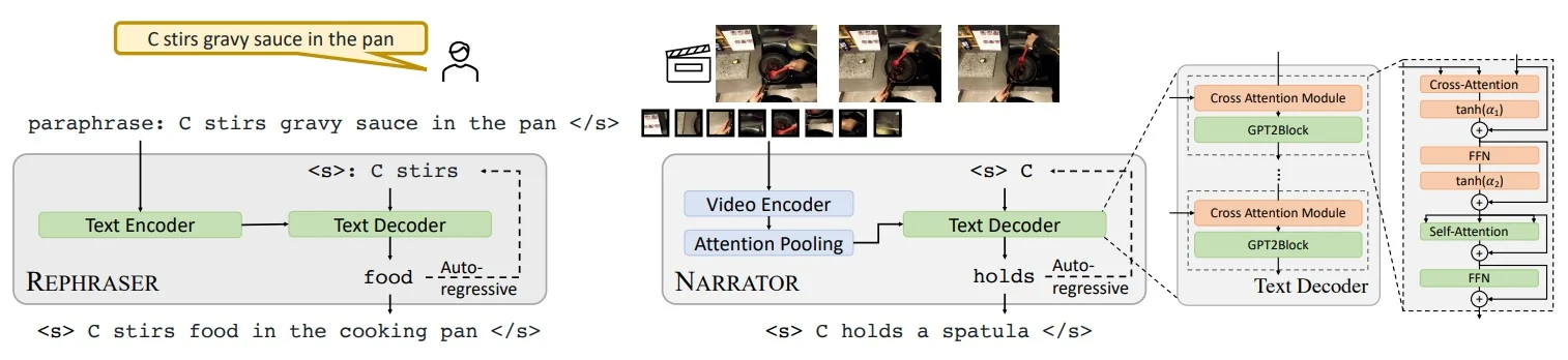
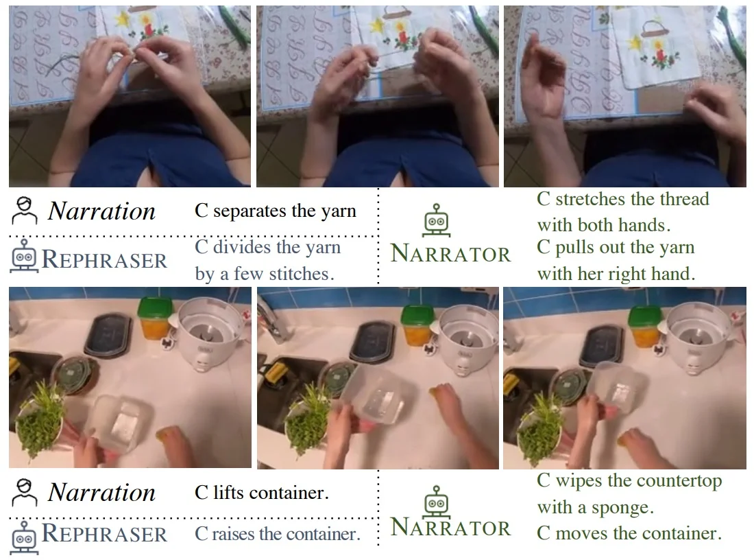
Pretraining schedule and input processing Pretraining on Ego4D runs for 5 epochs with AdamW, weight decay \(0.01\), fixed LR \(3{\times }10^{-5}\), mixed precision (FP16) and gradient checkpointing; total batch size reaches \(1024\) (e.g., \(32{\times }32\) or \(16{\times }64\) per-GPU setups). Videos are segmented into \(5\)-minute chunks with the short side scaled to \(288\); 4 frames are sampled uniformly within the clip window with standard random resized crops.
Experiments
Benchmarks and protocols Table 24.59 lists the downstream tasks used to evaluate LaViLa: egocentric multi-instance retrieval (EK-100 MIR), egocentric QA and temporal localization (Ego4D MCQ, NLQ), action recognition (EGTEA Gaze+, CharadesEgo), and third-person recognition (UCF-101, HMDB-51). Evaluations follow three standard protocols: zero-shot (ZS), finetuning (FT), and linear probing (LP).
| Dataset | Task | Egocentric | Metrics | Protocol |
|---|---|---|---|---|
| Epic-Kitchens-100 | MIR / CLS | Yes | mAP, nDCG / Top-1 | ZS, FT |
| Ego4D | MCQ / NLQ | Yes | Accuracy / Recall@N | ZS / FT |
| EGTEA Gaze+ | CLS | Yes | Top-1, Mean acc. | ZS, FT |
| CharadesEgo | CLS | Yes | Video-level mAP | ZS, FT |
| UCF-101 | CLS | No | Mean acc. | LP |
| HMDB-51 | CLS | No | Mean acc. | LP |
Headline results LaViLa establishes strong or state-of-the-art performance across first- and third-person settings by leveraging dense LLM narrations and a source-aware contrastive schedule [813]. On EK-100 MIR (Table 2 in [813]), ZS with TimeSformer-L (TSF-L) attains 40.0 mAP (V\(\rightarrow \)T) and 32.2 mAP (T\(\rightarrow \)V), averaging 36.1 mAP; FT reaches 54.7/47.1 mAP (avg. 50.9). On Ego4D (Table 3), LaViLa-L achieves 94.5% inter-video and 63.1% intra-video accuracy on MCQ, and R@1\(=\)12.05 at mIoU@0.3 on NLQ. On EGTEA (Table 4), FT with TSF-L yields 81.75% top-1 and 76.00% mean accuracy. On CharadesEgo (Table 5), ZS/FT mAP are 28.9/36.1. With third-person pretraining (Table 6), linear probing attains 88.1% on UCF-101 and 61.5% on HMDB-51.
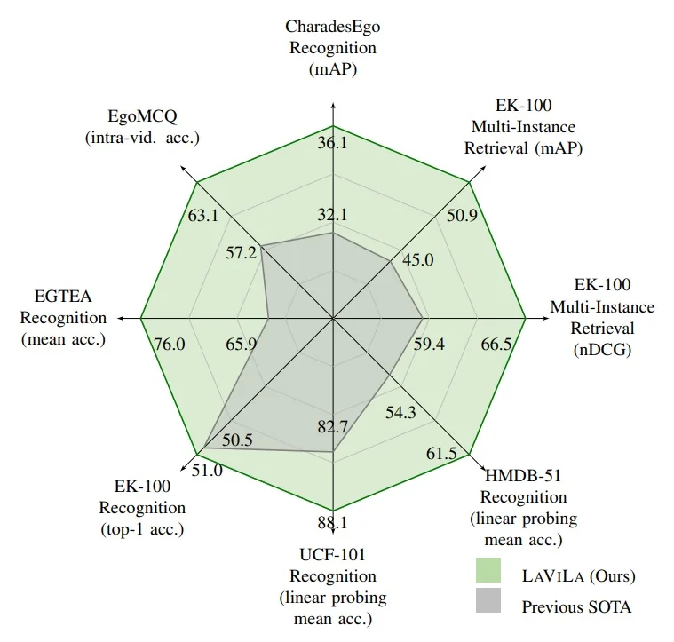
Summary of main experiments and ablations Pretraining uses roughly 4M \(\sim \)1 s narrated clips from Ego4D and evaluates zero-shot (ZS), finetuned (FT), and linear-probe (LP) settings across egocentric and third-person tasks [813].
- Narration quality and downstream effect. How quality is measured: On held-out Ego4D clips, NARRATOR outputs are compared to human references using standard captioning metrics—METEOR (0–1; matches content with synonym/fragment rewards), ROUGE-L (0–1; longest common subsequence overlap), and CIDEr (higher is better; consensus with multiple references). With GPT-2 XL as the NARRATOR, the paper reports METEOR \(0.289\), ROUGE-L \(0.530\), CIDEr \(0.940\), indicating fluent, on-topic descriptions at the same timestamps as the 1s clips. Why it matters: These dense, time-aligned sentences provide richer supervision than sparse clip labels or noisy ASR, yielding stronger video–text alignment. Observed effect: Using these narrations for pretraining correlates with better downstream retrieval on EK-100 MIR (e.g., mAP \(26.2\) with GPT-2 XL vs. \(24.3\) with a smaller GPT-2 and \(20.1\) with random-init GPT-2 XL), demonstrating that higher caption fidelity translates into better alignment [813].
- Epic-Kitchens-100 MIR (retrieval). EK-100 comprises long, egocentric cooking videos with many fine-grained actions; the Multi-Instance Retrieval task matches text queries to the correct short action segments across long videos and is scored by mAP/nDCG. With a TimeSformer-L backbone, ZS yields \(\sim 40.0\) mAP (video\(\rightarrow \)text) and \(\sim 32.2\) mAP (text\(\rightarrow \)video), and FT rises to \(\sim 54.7\) and \(\sim 47.1\) mAP, respectively, evidencing robust narration-supervised alignment in both directions [813].
- Ego4D QA and temporal localization. Ego4D includes multiple-choice QA (MCQ; inter-video / intra-video) and natural language queries (NLQ) that require pinpointing when a described event occurs. LaViLa improves MCQ accuracy (e.g., \(\sim 94.5\%\) inter-video and \(\sim 63.1\%\) intra-video) and boosts NLQ recall at fixed temporal IoU (e.g., R@1 at mIoU\(\,{=}\,0.3\) \(\sim 12.05\)), showing that dense narrations help the model learn to temporally ground text in long, first-person videos [813].
- Egocentric action recognition. On EGTEA Gaze+ and CharadesEgo, LaViLa attains strong ZS and FT results (e.g., EGTEA top-1 accuracy \(>{}80\%\) with TimeSformer-L; CharadesEgo ZS and FT mAP surpass prior contrastive/pretext methods), indicating that narration-aligned features transfer beyond retrieval to closed-set classification [813].
- Third-person generalization. Despite pretraining on egocentric footage, linear probing on trimmed third-person datasets confirms broader utility: with TimeSformer-L, UCF-101 and HMDB-51 achieve \(\sim 88\%\) and \(\sim 62\%\) accuracy, respectively, suggesting the learned representation is not tied to first-person viewpoints and generalizes to conventional action clips [813].
Ablations Ablations (Sec. 5.4; Tables 7–8 in [813]) isolate which design choices drive alignment quality. Unless noted, numbers reference EK-100 multi-instance retrieval (MIR) mAP on 1 s Ego4D clips as a proxy for video–text alignment.
- Narrator quality and LLM scale. What was tested: The NARRATOR used to create training captions was varied among (a) GPT-2 XL initialized from WebText and then visually conditioned via cross-attention, (b) a smaller GPT-2 (pretrained), and (c) GPT-2 XL with random initialization trained only on video captions. Quality was measured against human narrations with METEOR/ROUGE-L/CIDEr, and the downstream effect was measured by EK-100 MIR after using each narrator’s outputs for pretraining. Results: Pretrained GPT-2 XL yields the strongest captions (METEOR \(0.289\), ROUGE-L \(0.530\), CIDEr \(0.940\)) and the best retrieval (mAP \(26.2\)) versus the smaller GPT-2 (\(24.3\)) and random-init GPT-2 XL (\(20.1\)). Why it matters: Large, pretrained language priors generate more fluent and temporally specific narrations, producing a cleaner and denser supervision signal for contrastive alignment [813].
- Sampling strategy for narration. What is sampled: At generation time, the NARRATOR samples token sequences (full sentences) for each video clip. The study compares decoding methods: beam search (high-probability single phrasing) versus nucleus sampling (stochastic next-token draws from the top-p mass, here \(p{=}0.95\)), producing \(K{=}10\) alternative narrations per clip; a repeated-sampling variant increases this candidate pool further. Results: Nucleus sampling outperforms beam search (mAP \(29.7\) vs. \(27.9\)), and repeated sampling adds \(\sim {+}1.8\) mAP. Why it matters: Multiple diverse captions for the same clip cover alternative phrasings and event decompositions, improving robustness and generalization in contrastive training [813].
- Backbone capacity and input resolution. What was tested: TimeSformer-B \(\rightarrow \) TimeSformer-L \(\rightarrow \) TimeSformer-L@HR. Results: Consistent gains as capacity and resolution increase (mAP \(26.0 \rightarrow 29.7 \rightarrow 35.0\)). Why it matters: Stronger vision encoders exploit dense narration supervision to capture finer motion and interactions, amplifying transfer [813].
- Clip length and narration density. What was tested: Durations \(\{0.5\,\mathrm {s},1\,\mathrm {s},2\,\mathrm {s}\}\) and sentences per clip (sparse \(N{=}1\) vs. dense \(N{\approx }10\)). Results: \(1\) s clips with dense narrations perform best, typically \({+}2\)–\({+}4\) mAP over sparser/longer settings. Why it matters: Short, action-focused clips with several sentences balance coverage and precision, yielding clearer temporal grounding [813].
- Semi-supervised efficiency. What was tested: Training with \(10\%\)–\(100\%\) of the narrated Ego4D data. Results: Using only \(50\%\) of the narrated data remains competitive with full-label baselines on EK-100 MIR and Ego4D tasks. Why it matters: LLM narrations provide label-efficient supervision, sustaining strong performance under reduced human annotation budgets [813].
- Temperature setting in the contrastive loss. What was tested: Fixed temperature versus learned or source-specific temperatures. Results: A single fixed temperature (e.g., \(\tau {=}0.07\)) is most stable and yields the best overall metrics in this setting. Why it matters: Simple scaling avoids over-weighting noisier pseudo-captions or under-weighting clean paraphrases, leading to smoother optimization [813].
Limitations and future directions
Observed constraints LaViLa learns strong video–text alignment from dense narrations, but several boundaries remain clear in the original paper. [813]
- Narration quality and bias. Supervision ultimately inherits the style and limitations of narrated text (human or LLM-generated). Despite careful prompting and sampling, narrations can be repetitive, partially off-topic, or unevenly distributed across events, which may cap downstream temporal precision [813].
- Alignment over generation. The dual-encoder is optimized with a contrastive objective for retrieval and recognition. It is not trained for open-ended text generation, step-by-step explanations, or multi-turn dialogue; those abilities require an autoregressive language modeling objective and an explicit interface to a generative LLM [813].
- Clip-level horizon. Training focuses on short clips paired with sentences. This yields robust local alignment but leaves long-range reasoning (ordering, causality, procedure tracking) underconstrained unless additional mechanisms summarize or chain evidence over time [813].
- Modality scope. The method centers on video–text. Audio is not explicitly modeled in the pretraining objective, so grounding to acoustic events or off-screen sound requires further extensions [813].
- Domain and language coverage. Narrations are predominantly English and egocentric in the main setup, which can introduce domain or language bias when transferring to third-person or multilingual settings [813].
Future work These constraints suggest clear next steps for narration-supervised pretraining.
- Audio-visual grounding. Incorporate ASR and raw audio features with timestamped alignment so captions can reference sounds and speech, not only visuals, improving moment retrieval and event disambiguation.
- Instruction-tuned conversational layers. Add a lightweight connector from the frozen video encoder to a pretrained LLM and fine-tune with multimodal instructions to enable open-ended answers and multi-turn dialogue on video.
- Long-context summarization. Introduce hierarchical pooling or memory to aggregate many clips into compact tokens, enabling hour-scale reasoning and timeline queries without prohibitive compute.
- Multilingual and broader domains. Generate and curate narrations across languages and domains to reduce bias and improve transfer, with calibration or filtering to control LLM style drift.
- Quality control of pseudo-labels. Use confidence estimates, agreement checks, or retrieval-based filtering to keep narrated supervision precise while scaling data.
Bridge to instruction-tuned video–LLMs Narration-supervised alignment in LaViLa supplies dense, scalable supervision that yields a strong video encoder for downstream use. [813] This makes a natural foundation for instruction-tuned video–LLMs such as Video-LLaMA, where a pretrained video encoder is coupled to a generative LLM via a lightweight connector and adapted on conversational data to add open-ended reasoning and dialogue over video [787, 105].
Enrichment 24.9.2: Video-LLaMA 1: Instruction-Tuned Video LLM
Motivation
Why audio–visual LLMs? Most multimodal LLMs circa early 2023 target either image–text [343, 377, 823] or audio–text [256], leaving video under-served and typically silent.1 Video-LLaMA1 addresses two gaps for video understanding: (i) modeling temporal change in visual scenes, and (ii) integrating audio with vision in a single LLM-centric framework.
Design goal Leverage strong, frozen foundation encoders for vision and audio, plus a frozen LLM, and learn only light adapters to connect modalities, preserving priors while enabling efficient instruction tuning.
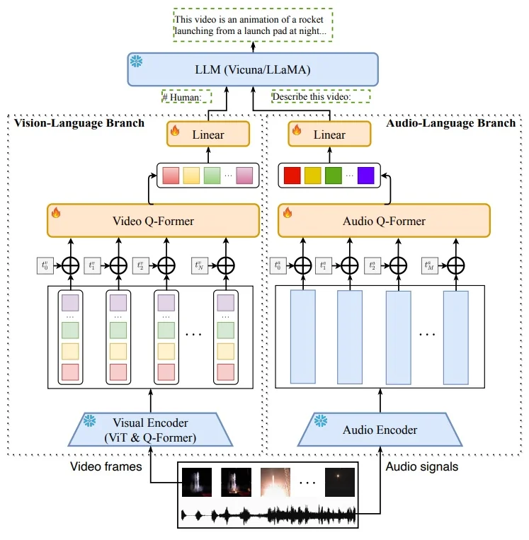
Method: Multi-Branch Cross-Modal Training with Q-Formers
Problem setup and notation Given a video with \(N\) frames and waveform audio split into \(M\) short segments, the goal is to produce a response \(\hat {y}\) to a user instruction \(y^{\mbox{instr}}\) conditioned on video and audio. Video-LLaMA1 constructs two query sequences: \(\hat {\mathbf {v}}\in \mathbb {R}^{k_V\times d}\) from frames and \(\hat {\mathbf {a}}\in \mathbb {R}^{k_A\times d}\) from audio, projects them into the LLM embedding space, and concatenates them with tokenized \(y^{\mbox{instr}}\) as a soft prompt to drive the frozen LLM’s next-token generation (See Fig. 24.99).
Vision–Language branch Per-frame features are extracted by a frozen image encoder (ViT/G from EVA-CLIP within BLIP-2), yielding \(V=[\mathbf {v}_1,\ldots ,\mathbf {v}_N]\), where \(\mathbf {v}_i\in \mathbb {R}^{K_f\times d_f}\). Temporal position embeddings are added across frames. A Video Q-Former (same architecture as BLIP-2’s Query Transformer) aggregates across time via learnable queries to produce \(k_V\) video embedding vectors \(\hat {\mathbf {v}}\in \mathbb {R}^{k_V\times d_v}\), followed by a linear projector mapping into the LLM token space to form video query tokens. These tokens are concatenated with text embeddings as a visual soft prompt to the frozen LLM.
Audio–Language branch Audio is uniformly segmented into \(M\) chunks (typically \(2\) s each), converted into log-Mel spectrograms (128 Mel bins), and fed to a frozen ImageBind audio encoder to obtain a sequence of segment embeddings \(A=[\mathbf {a}_1,\ldots ,\mathbf {a}_M]\), with \(\mathbf {a}_m\in \mathbb {R}^{d_a}\) [179]. What is ImageBind? ImageBind is a multimodal foundation model trained with contrastive learning so that images, text, audio, and other modalities share a single embedding space. It uses images as a pivot: audio is aligned to images and text is aligned to images, which binds audio and text transitively (e.g., a “bark” sound and the word “dog” end up close), providing semantically grounded audio features without extra audio–text supervision [179].
An Audio Q-Former (a lightweight, trainable query-based Transformer) with temporal position embeddings then attends over \(A\) and compresses the variable-length sequence into a fixed set of \(k_A\) audio queries, \[ \hat {\mathbf {a}}\in \mathbb {R}^{k_A\times d_a}, \] where the \(k_A\) learnable query tokens aggregate salient temporal cues. A final linear projector \(W_a\in \mathbb {R}^{d_a\times d_{\mbox{LLM}}}\) maps these queries into the LLM token space, \[ \mathbf {z}^{(a)}=\hat {\mathbf {a}}\,W_a \in \mathbb {R}^{k_A \times d_{\mbox{LLM}}}, \] yielding audio query tokens that are concatenated with the user prompt (and, when present, visual tokens) to condition the frozen LLM for audio-grounded video dialogue.
Training curriculum Video-LLaMA1 follows a staged, dual-branch curriculum that first teaches the adapters to describe from visual/audio inputs and then sharpens instruction following for dialogue. Crucially, the large backbone encoders (vision: BLIP-2’s ViT-G/14 from EVA-CLIP; audio: ImageBind) and the language model (LLaMA/Vicuna) are kept frozen; only the lightweight bridges (Video/Audio Q-Formers, temporal position embeddings, and linear projectors) are optimized in all stages [787]. This design “guides the frozen LLM” using learned query tokens (soft prompts), and the paper’s “fine-tuning” wording refers to adapting these bridges with different datasets, not unfreezing the LLM.
- (a)
- Vision pre-training (video/image\(\to \)text generation). Using large vision–caption corpora (WebVid-2M short clips; filtered CC595k image captions), the frozen BLIP-2 vision encoder produces frame features. Learnable temporal position embeddings are added to inject ordering over frames, and a Video Q-Former aggregates them into a fixed number of video query tokens. A linear projector maps these tokens to the LLM embedding space; concatenating them with text inputs prompts the frozen LLM to generate captions. This stage prioritizes broad visual knowledge despite caption noisiness [787, Sec. 2.1–2.2].
- (b)
- Vision instruction tuning (image/video dialogue). The same visual adapters are further trained on high-quality instruction data (e.g., MiniGPT-4 image descriptions, LLaVA image instructions, Video-Chat video instructions) so that the frozen LLM better follows prompts, answers questions, and maintains multi-turn coherence when conditioned on the learned video tokens [787, Sec. 2.2].
- (c)
- Audio pre-training (audio\(\to \)text via pivot). Due to scarce audio–text pairs, the audio branch leverages a frozen ImageBind audio encoder to produce segment features that already live in a multimodal space aligned with images/text [179]. Uniform 2 s chunks are converted to 128-bin log-Mel spectrograms and encoded into a sequence \(A=[\mathbf {a}_1,\ldots ,\mathbf {a}_M]\). An Audio Q-Former with temporal position embeddings fuses \(A\) into a fixed set of audio query tokens, which are projected to the LLM space. Training uses the same vision–text data as a pivot: the loss is applied on text generation while conditioning the LLM on audio-side tokens whose features are aligned to vision via ImageBind. This yields zero-shot audio understanding at inference, even without direct audio–text supervision [787, 179, Sec. 2.1.2, 2.2.2].
Video-LLaMA1 uses a single frozen image encoder (the BLIP-2 vision tower) for both images and videos by treating an image as a 1-frame video. Concretely: (i) for a static image, the encoder runs once to produce patch tokens for that single frame; (ii) for a video, \(N\) frames are uniformly sampled and each frame is encoded independently by the same tower, yielding a sequence of per-frame tokens; (iii) learnable temporal position embeddings are added to mark frame order; and (iv) a Video Q-Former cross-attends over this ordered sequence and compresses it into a fixed number of visual query tokens, which are then projected into the LLM embedding space. This unified pathway avoids modality-specific encoders while the temporal embeddings and the Q-Former supply the missing “when” signal and spatio-temporal aggregation absent from a purely image-trained backbone [787, Sec. 2.1.1–2.2].
Positional encoding (vision & audio) Because the frozen encoders do not model time, Video-LLaMA1 injects learnable temporal position embeddings after feature extraction: per-frame (vision) and per-segment (audio) embeddings are added before the corresponding Q-Formers, enabling temporal reasoning without unfreezing the backbones [787, Sec. 2.1.1–2.1.2].
Learning objective (unified view) All stages optimize the standard autoregressive language-modeling loss (next-token negative log-likelihood) on the frozen LLM, conditioned on the concatenation of modality query tokens and textual context: \[ \mathcal {L}_{\mathrm {LM}} \,=\, -\sum _{t=1}^{T} \log p\!\left ( w_t \,\middle |\, w_{<t},\, Q_v \ \mbox{and/or}\ Q_a,\, c \right ), \] where \(Q_v\)/\(Q_a\) are the fixed-length video/audio query tokens produced by the Q-Formers and projected to the LLM space, \(c\) is the text context (caption/instruction), and \(w_t\) are target tokens. No extra losses are introduced; the adapters learn to act as soft multimodal prompts that elicit correct generations from a frozen LLM [787, Sec. 2.2].
Intuition and roles Q-Formers act as learnable compressors that query and distill dense frame or audio features into a small, fixed set of tokens that an LLM can reliably consume, mirroring BLIP-2 for images but extended temporally (video) and across modality (audio). ImageBind provides the audio branch with a pragmatic route to align with text even without abundant audio–text pairs. Together, they let a frozen LLM “see and hear” with minimal new parameters.
Architecture & Implementation Details
Backbones and frozen parts Vision uses the BLIP-2 visual stack: EVA-CLIP ViT-G/14 + Q-Former (both frozen). Audio uses the frozen ImageBind audio encoder. The LLM is Vicuna/LLaMA (frozen). Trainable parts are: temporal position embeddings, Video Q-Former, Audio Q-Former, and small linear projectors to the LLM token space.
Video tokens Each frame yields \(K_f\) image tokens; temporal position embeddings index frames; Video Q-Former outputs \(k_V\) video query tokens. A linear projector maps these into the LLM embedding dimension; tokens are then prepended/concatenated to text embeddings as a soft prompt.
Audio tokens Audio is chunked, Mel-spectrogrammed, embedded via ImageBind, fused by the Audio Q-Former into \(k_A\) tokens, then projected to the LLM space and concatenated alongside video tokens.
GEMINI additions (intuitive recap) The dual-branch design feeds a central LLM with what it sees (Video Q-Former summary of frames) and what it hears (Audio Q-Former summary of audio). The LLM then produces responses grounded in both modalities, e.g., recognizing a rocket launch and describing engine roar (See Fig. 24.99).
Experiments and Ablations
Qualitative capabilities Video-LLaMA1 enables multi-turn audio–visual dialogue: (a) answering questions grounded jointly in background sound and visual content; (b) describing actions over time (temporal reasoning across frames); (c) analyzing single images; and (d) recognizing well-known landmarks (Figure 24.100). These examples illustrate how the model combines the vision and audio branches to condition a frozen (or LoRA-adapted) LLM for grounded responses [787].
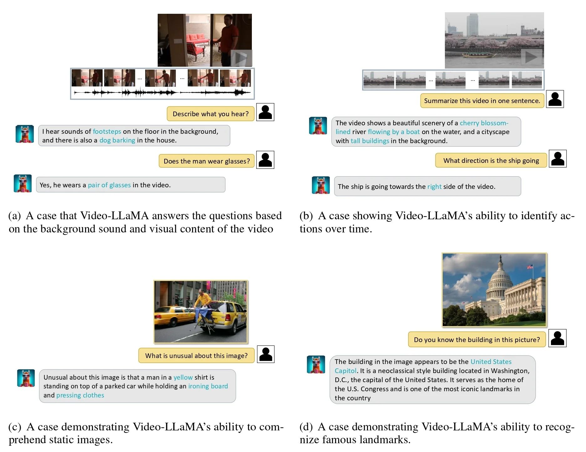
Tasks and metrics (at a glance) Evaluation follows standard video–language setups [787]: (i) Video QA on MSRVTT-QA and ActivityNet-QA (reported as answer accuracy); (ii) Video captioning on MSVD/MSRVTT (reported with CIDEr/BLEU/METEOR); and (iii) Retrieval on MSRVTT (reported with Recall@K). The paper focuses on zero-shot and instruction-tuned settings, highlighting gains attributable to the staged curriculum.
Training stages and ablations A staged curriculum underpins the stability and performance of Video-LLaMA1, with pre-training for grounding followed by instruction tuning for conversational ability; empirical studies in [787, Sec. 2.1–2.3, 4] confirm the contribution of each step.
- Vision caption pre-training \(\rightarrow \) broad visual grounding. Using large, weakly supervised corpora (WebVid-2M video clips and filtered image–caption sets), the Video Q-Former and projector learn to produce a compact set of visual query tokens that condition the frozen LLM to generate captions, yielding stronger descriptive ability and better retrieval-style baselines than adapter-free or frozen-feature variants. Ablation: Query-based cross-attention with temporal position embeddings outperforms naive frame pooling for video QA, indicating a learnable bottleneck is more effective for distilling spatio–temporal cues into the LLM token budget [787, Sec. 2.1, 4]. .
- Instruction tuning \(\rightarrow \) QA accuracy and multi-turn dialogue. Fine-tuning the same visual adapters together with a lightweight LLM adaptation on clean image/video instruction–response data improves answer relevance and stabilizes multi-turn consistency compared to caption-only training, showing that instruction-formatted supervision is required to elicit conversational behaviour. Ablation: Models trained only on captions underperform on question answering and dialogue coherence despite solid visual grounding [787, Sec. 2.3, 4]. .
- Audio pivoting \(\rightarrow \) zero-shot audio understanding. With a frozen ImageBind audio encoder, the Audio Q-Former is trained via a vision–text pivot to produce audio query tokens aligned to the LLM space without paired audio–text datasets, enabling audio-aware responses for questions that depend on background sounds. Ablation: The pivoted audio branch outperforms variants that omit audio, providing a practical and data-efficient route to audio grounding [787, Sec. 2.2, 4].
Relative to LaViLa (narration-supervised dual-encoder optimized for alignment and retrieval), Video-LLaMA1 is a generative, instruction-tuned audio–visual language model: it supports free-form answers, multi-turn dialogue, and audio grounding while reusing frozen perception backbones through Q-Formers. Compared to image-first instruction models (e.g., BLIP-2, LLaVA, MiniGPT-4), Video-LLaMA1 adds temporal modeling (frame sequences with temporal embeddings and a Video Q-Former) and an explicit audio branch via ImageBind, enabling questions that depend on motion and sound. Modality coverage is summarized in Table 24.60, and unified follow-ups (e.g., LLaVA-OneVision) are discussed in Sec. Enrichment 24.7.2.
Limitations and Future Directions
Observed constraints Video-LLaMA1 is an early-stage prototype. The paper highlights: (1) performance is bounded by the scale/quality of current training data; (2) limited ability to handle long videos due to compute and fixed token budgets; and (3) hallucinations inherited from the frozen LLM.
Future work The authors call for higher-quality audio–video–text alignment data, longer-context modeling for movies/TV-scale inputs, and mitigation strategies for hallucination. These directions naturally motivate successors (Video-LLaMA2/3) that extend clip length, strengthen audio–visual synchronization, and scale instruction data and adapters (see next subsections in this enrichment).
Enrichment 24.9.3: Video-LLaMA 2: Enhanced Understanding, Efficiency
Overview and motivation Video-LLaMA2 [105] extends Video-LLaMA1 by replacing the Q-Former connector with a compute-efficient Spatial–Temporal Convolution (STC) connector and by introducing a stronger audio pathway and staged audio–visual training. The goals are: (i) preserve local spatial–temporal structure while reducing video tokens; (ii) scale to longer clips without exploding token budgets; and (iii) strengthen audio understanding via a modern audio encoder (BEATs) and curriculum. The design keeps modality encoders frozen and lets a lightweight connector plus an LLM handle fusion and reasoning, improving robustness and efficiency for instruction-following video chat and QA.
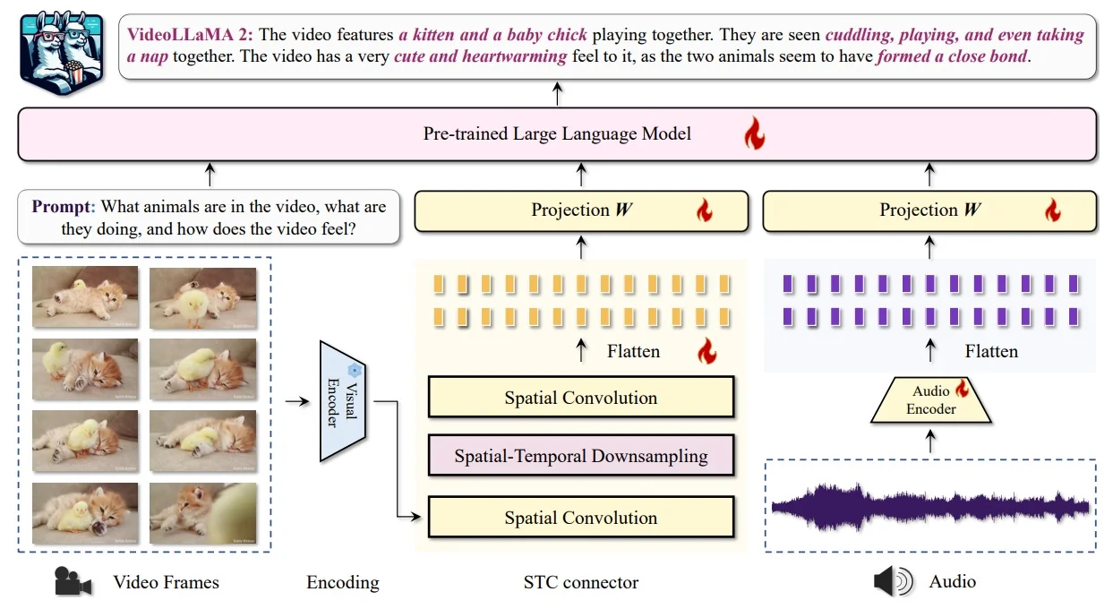
Method
Modality branches (concise) Video-LLaMA2 feeds a (frozen–decoder) LLM with compact tokens produced by two parallel branches [105, Sec. 2]:
- Vision. Uniformly sampled frames \(\rightarrow \) frozen CLIP ViT-L/14 (per-frame features) \(\rightarrow \) STC connector (RegStage \(\rightarrow \) 3D conv with downsampling \((t,s,s)\) \(\rightarrow \) RegStage) \(\rightarrow \) small MLP projector to LLM tokens [105, Sec. 2.1].
- Audio. Waveform \(\rightarrow \) log-Mel spectrograms (128 bins) \(\rightarrow \) frozen BEATs encoder \(\rightarrow \) two-layer MLP to LLM tokens (no Audio Q-Former) [105, Sec. 2.2].
Tokens from both branches are concatenated with the text prompt and passed to the LLM for autoregressive generation.
STC connector: step-by-step mechanics and intuition Primer on RegStage. RegStage is the per-stage building block from the RegNet family [515] (implemented in timm and invoked in the paper’s pseudo-code), used here purely for spatial refinement on each frame [105, Alg. 1, Sec. 2.1]. Concretely, a RegStage stacks several lightweight 2D residual bottleneck blocks (conv \(\rightarrow \) norm \(\rightarrow \) activation, optional squeeze-and-excitation and/or group convolutions), with a fixed channel width across the stage and an optional stride in the first block for spatial downsampling. It does not mix information across time—every operation is intraframe—so it functions as a per-frame “detail enhancer” that sharpens edges, textures, and small objects before (and after) the temporal aggregation step in STC.
Why RegStage vs. an ad-hoc 2D stack? RegNet’s blocks arise from a regular design space discovered by large-scale network design exploration [515]: channel widths evolve by a simple quantized linear rule, depth/width are balanced per stage, and the block recipe remains constant. This regularity yields predictable compute/accuracy scaling and strong accuracy-per-FLOP at a given budget, whereas “irregular” CNN stacks (arbitrary kernel/width changes per layer) tend to be harder to scale efficiently. In Video-LLaMA2, this makes RegStage an ideal choice around the single 3D aggregation layer: it is (i) frame-local—preserving temporal order for the downstream 3D step; (ii) parameter- and FLOP-efficient—suited to long clips; and (iii) detail-retentive—its pre/post spatial filtering mitigates the blurring that temporal downsampling can introduce [105, Sec. 2.1].
Let \(F \in \mathbb {R}^{T \times H' \times W' \times D_v}\) denote per-frame features from the frozen ViT (one image per frame). The STC (RegStage \(\rightarrow \) Conv3D \(\rightarrow \) RegStage) transforms \(F\) into an order-aware token sequence \(Q_v\) for the LLM:
- (1) Pre-aggregation spatial interaction (RegStage #1). Apply a RegStage independently on each frame to strengthen intraframe structure: \[ F_1 = \mathrm {RegStage}_1(F). \] Intuition. This step sharpens spatial details before any temporal mixing, so that subsequent compression does not wash out fine cues needed for OCR, small objects, or delicate hand-object interactions [105, Sec. 2.1].
- (2) Spatio-temporal aggregation with explicit downsampling (3D Conv). Treat the sequence as a 3D volume and aggregate with a single 3D convolution configured to downsample by factors \((t,s,s)\) along time/space: \[ F_2 = \mathrm {Conv3D}_{(t,s,s)}(F_1). \] This reduces the lattice roughly from \((T,H',W')\) to \(\big (\lceil T/t\rceil ,\lceil H'/s\rceil ,\lceil W'/s\rceil \big )\) while encoding short-range motion and local temporal context. Intuition. A 3D kernel “looks” at small space–time cubes and encodes what changes, where, and when instead of averaging away motion; explicit \((t,s,s)\) makes the token budget predictable for long clips [105, Sec. 2.1, Tab. 1].
- (3) Post-aggregation refinement (RegStage #2). Apply a second RegStage on the downsampled volume: \[ F_3 = \mathrm {RegStage}_2(F_2). \] Intuition. This “cleanup” stage restores spatial sharpness and reduces artifacts introduced by aggressive downsampling, yielding more discriminative tokens for the LLM [105, Sec. 2.1].
- (4) Projection to LLM tokens (MLP). Flatten the 3D lattice into a sequence and map each vector to the LLM embedding with a small MLP: \[ Q_v = \mathrm {MLP}\!\big (\mathrm {Flatten}(F_3)\big ) \in \mathbb {R}^{K \times d_{\mathrm {LLM}}}, \] where \(K \approx \lceil T/t\rceil \!\cdot \! \lceil H'/s\rceil \!\cdot \! \lceil W'/s\rceil \) is the resulting visual token count set by \((t,s,s)\) (e.g., the paper often uses \((2,2,2)\)). The sequence order follows scanline-in-time (preserving chronology), and \(Q_v\) is concatenated with text (and optional audio tokens) for generation [105, Sec. 2.1].
Why this “sandwich” works. A plain stack of 3D convolutions can over-mix space and time too early, blurring fine spatial structure; the RegStage–Conv3D–RegStage design deliberately separates delicate and dedicated spatial refinement (before/after) from temporal aggregation (middle), preserving locality while encoding motion. Ablations favor this configuration—especially with downsampling \((2,2,2)\)—for superior MC-VQA averages under tighter token budgets [105, Tab. 1].
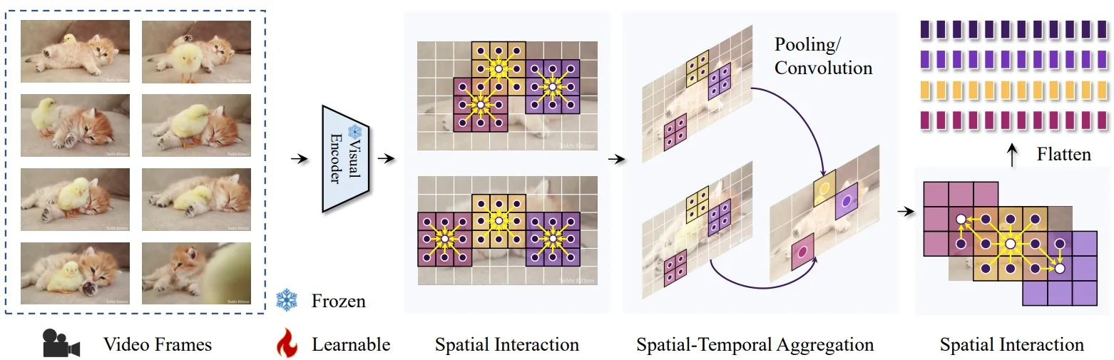
Why STC instead of a plain 3D CNN or a Q-Former?
- Versus a plain 3D CNN stack. Repeated 3D mixing tends to smear fine details by coupling space and time at every layer; STC confines temporal aggregation to one explicit step and uses RegStage to protect and then restore spatial fidelity, improving accuracy at a comparable or smaller token budget [105, Sec. 2.1, Tab. 1].
- Versus the V1 Q-Former. Attention-based querying is flexible but token-hungry on long sequences and may disturb chronological order via learned resampling; STC preserves frame order by construction, offers deterministic \((t,s,s)\) reduction, and scales linearly with clip length—yielding better MC-VQA averages under tighter budgets in the paper’s comparison [105, Sec. 2.1, Tab. 1].
Implementation of STC in Python (from the paper)
import torch.nn as nn
from timm.models.regnet import RegStage


class STCConnector(nn.Module):
    def __init__(self, config, depth, mlp_depth):
        # Temporal and spatial downsampling factor
        td, sd = config.td, config.sd
        # Input and output hidden dimension
        in_size, out_size = config.in_size, config.out_size
        # The first RegStage block
        self.s1 = RegStage(depth=depth, in_chs=in_size, out_chs=out_size)
        # Conv3D downsampler
        self.downsampler = nn.Conv3d(in_channels=out_size,
                                     out_channels=out_size,
                                     kernel_size=(td, sd, sd))
        # The second RegStage block
        self.s2 = RegStage(depth=depth, in_chs=out_size, out_chs=out_size)
        self.proj = build_mlp(mlp_depth, out_size, out_size)

    def forward(self, x):
        x = self.s1(x)
        x = self.downsampler(x)
        x = self.s2(x)
        x = self.proj(x)
        return x
Design principles. The authors avoid resampler-style connectors to keep token order consistent for the autoregressive LLM; introduce explicit 3D downsampling to control token count; and use RegStage blocks around the downsampler to compensate for losses from compression [105, Sec. 2.1, Fig. 2].
Training signal and integration All connector parameters (RegStage blocks, 3D conv, MLP) are optimized only through the standard next-token LM loss in captioning/QA/instruction formats, with visual/audio encoders frozen and the LLM optionally adapted with parameter-efficient tuning during instruction stages [105, Sec. 3]. This keeps the connector small, order-aware, and compute-efficient while enabling strong temporal modeling at inference time.
Key changes vs. V1 (what changed and why) Video-LLaMA2 replaces the V1 Video Q-Former with a convolutional STC to scale to long clips under tight token budgets while keeping the sensory encoders frozen [105, Sec. 2]. The shift is motivated by three practical needs:
- Chronology by construction. A single 3D convolution aggregates adjacent frames directly, preserving temporal order without learned resampling that can shuffle/sparsify frames in attention-based connectors [105, Sec. 2.1].
- Deterministic token control. Explicit downsampling with stride \((t,s,s)\) (e.g., \((2,2,2)\)) reduces tokens early and predictably, enabling longer contexts with stable memory/latency and better accuracy–efficiency trade-offs [105, Sec. 2.1, Tab. 1].
- Detail preservation around compression. Lightweight RegStage blocks before/after the 3D step act as spatial “sharpen/cleanup” modules, mitigating the blur introduced by temporal downsampling and improving MC-VQA averages at comparable or smaller token budgets [105, Sec. 2.1, Tab. 1].
Audio branch update. The ImageBind-pivoted Audio Q-Former in V1 is replaced with a frozen BEATs encoder plus a small MLP projector, followed by a staged audio \(\rightarrow \)audio+video curriculum. This simplifies alignment, strengthens A/V synchronization, and improves audio-aware reasoning under limited token and compute budgets [105, Sec. 2.2, 3.2].
Architecture and implementation details Vision backbone. Image-level CLIP ViT-L/14 processes frames independently at \(336{\times }336\), then the STC connector aggregates across time and space, producing a compact set of video tokens for the LLM [105, Sec. 2.1]. Audio backbone. BEATs encodes fbank (log-Mel) spectrograms; a 2-layer MLP aligns to the LLM dimension [105, Sec. 2.2]. LLM. Mistral-7B-Instruct and Mixtral-Instruct are used as decoders; modality encoders remain frozen; the connector and projector are optimized, and instruction tuning is applied for dialogue [105, Sec. 2].
Training curriculum (i) Vision–language pre-training. Filtered web-scale image/video–text data are used with frozen encoders and LLM; only the STC connector is optimized via token-level cross-entropy (next-token LM loss) [105, Sec. 3.1.1]. The curated recipe keeps \(12.2\)M pairs from \(103\)M candidates (WebVid-10M \(4.0\)M; Panda-70M \(2.8\)M; VIDAL-10M \(2.8\)M; InternVid-10M \(650\)K; CC-3M \(595\)K; DCI \(7.8\)K) [105, Tab. 2]. (ii) Multi-task fine-tuning. Simultaneous captioning, classification, VQA, and instruction tuning over \(\approx 1.35\)M samples (Video–Text \(488\)K; Image–Text \(746\)K; Text-only \(120\)K) [105, Sec. 3.1.2, Tab. 3]. (iii) Audio & AV curriculum. Three stages totaling \(\sim 1.9\)M: audio-only pre-train (\(\sim 400\)K), audio instruction (\(\sim 698\)K), and joint audio–video (\(\sim 836\)K) for synchronization and AV reasoning [105, Sec. 3.2, Tab. 4]. Objective. All stages use standard autoregressive LM loss conditioned on visual/audio tokens and text, with encoders frozen and connector/projector (and LLM adapters during instruction tuning) updated [105, Sec. 3].
Experiments and Ablations
STC Ablations A controlled sweep (8 frames, Video-LLaVA data) tests spatial interaction (RegStage vs. none) and aggregation (2D/3D pool/conv) under explicit downsampling. The optimal configuration is RegStage ✓ + 3D Conv with \((2,2,2)\) downsampling, yielding Avg. 45.1 on MV-Bench, EgoSchema, ActivityNet-QA with 576 tokens (green row, Table 1). Weaker alternatives include 2D Pool with \((1,2,2)\) at Avg. 44.4 and 1152 tokens (token-hungry), and 3D Conv with \((2,2,2)\) but no RegStage at Avg. 43.1 and 576 tokens (detail loss). Insight: A single, early 3D fusion step captures motion efficiently, while pre/post RegStage recovers spatial sharpness, giving +2–4% QA over 2D or plain 3D variants and enabling long-clip scaling without context explosion [105, Tab. 1].
Data Recipe Overview Pre-training filters 103M raw pairs to 12.2M video/image-text pairs (e.g., WebVid-10M: 4.0M; Panda-70M: 2.8M; see Table 2). Multi-task fine-tuning uses 1.35M samples (video-text 488K, image-text 746K, text-only 120K; Table 3). The audio curriculum totals 1.9M instances (400K audio pre-train, 698K audio instruction, 836K audio + video joint; Table 4). Insight: Heavy filtering (11.8% retention) prioritizes quality over raw scale, improving transfer compared with unfiltered mixtures [105, Tab. 2–4].
Multiple-Choice VQA and Perception With 16 frames and a 7B decoder, Video-LLaMA2 reports EgoSchema 51.7%, Perception-Test 51.4%, MV-Bench 54.6%, VideoMME 47.9/50.3%, and MSVC 2.53/2.59. Using 8 frames slightly reduces performance (e.g., MV-Bench 53.4%), while scaling the decoder to Mixtral 8 \(\times \) 7B (\(\approx \)72B) lifts scores to 63.9/57.5/62.0% on EgoSchema/Perception-Test/MV-Bench and 61.4/63.1% on VideoMME (MSVC 2.61/2.61), under the same protocol [105, Tab. 5].
Open-Ended Video QA For MSVD and ActivityNet-QA (accuracy/score), the 7B model attains 70.9/3.8 and 50.2/3.3. On the Video-ChatGPT human rubric, it scores 3.16/3.08/3.69/2.56/3.14 for Correctness, Detail, Context, Temporal/Consistency [105, Tab. 6]. Insight: Performance is competitive with image-first baselines on MSVD while showing stronger temporal judgments, consistent with STC’s motion preservation.
Audio QA On audio-only QA, Video-LLaMA2-7B reaches Clotho-AQA 70.11%, TUT2017 78.40%, and VocalSound 93.19% using \(\sim \)4k hours of audio, rivaling models trained on orders of magnitude more data (e.g., Qwen-Audio 7B at 57.90/64.90 with \(\sim \)137k hours) [105, Tab. 7]. Insight: The BEATs + MLP path is data-efficient for audio grounding.
Open-Ended Audio–Video QA With joint audio–video instruction, the 7B model achieves MUSIC-QA 79.2%, AVSD 57.2%, and VGGSound 70.9% on \(\sim \)1.8M pairs, surpassing prior open-source systems under comparable settings [105, Tab. 8]. Insight: The staged audio \(\rightarrow \) AV curriculum tightens cross-modal synchronization for fine-grained reasoning.
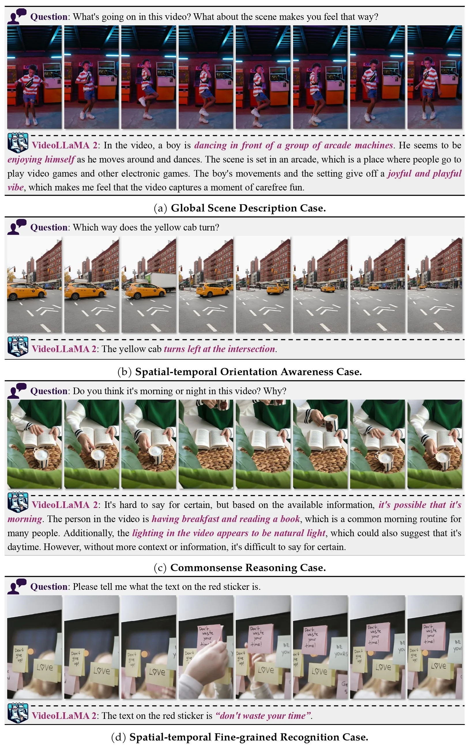
Limitations and future directions Video-LLaMA2 acknowledges several open challenges that shape the roadmap for video LLMs [105, Sec. 3–5]:
- Long-context scaling. Even with STC downsampling, reasoning beyond tens of seconds is constrained by the LLM’s context window and token budget; maintaining narrative coherence over minutes remains difficult under fixed compute and latency budgets.
- Fine-grained temporal precision. Aggressive \((t,s,s)\) reductions can blur boundaries of short, sequential actions (e.g., micro-gestures), suggesting a need for adaptive or multi-rate temporal modeling.
- Audio–visual synchronization. Joint training improves sync but still trails specialized AV systems on tightly coupled events (onset/offset, lip-speech alignment), indicating room for stronger cross-modal alignment objectives and curricula.
- LLM choice and data bias. The chosen decoders (Mistral/Mixtral) and filtered web corpora can limit domain robustness, multilingual coverage, and calibration under distribution shift; broader, curated instruction data and multilingual AV resources are needed.
Where next? Promising directions include hierarchical long-video memory and tiling, adaptive multi-rate temporal adapters, explicit AV alignment losses/heads, and larger, more diverse instruction datasets with multilingual audio and video. These themes naturally motivate the next model in this series: Video-LLaMA3, covered next, which explores longer contexts, finer temporal localization, and tighter audio–visual coupling while preserving token efficiency.
Enrichment 24.9.4: Video-LLaMA 3: Frontier Multimodal Foundation Models
Motivation
A vision-first redesign Video-LLaMA2 paired AnyRes tiling with a uniform spatio–temporal connector (STC) to squeeze long clips into an LLM context, but the grid remained rigid: tiling could distort aspect ratios and inflate tokens for simple scenes, while uniform downsampling tended to blur high–frequency detail (e.g., thin chart lines, small OCR text). Near-duplicate frames still consumed substantial budget [105]. Video-LLaMA3 reframes the pipeline around visual fidelity first, efficiency second: make the vision encoder genuinely resolution–agnostic so images and frames are ingested at native geometry, then treat a video as a sequence of correlated images and budget tokens toward changes rather than static redundancy [782]. In practice, that means any-resolution tokenization for spatial detail, a simple textualized interface (separators and timestamps) for temporality, and content-aware savings that extend the effective horizon without sacrificing detail.
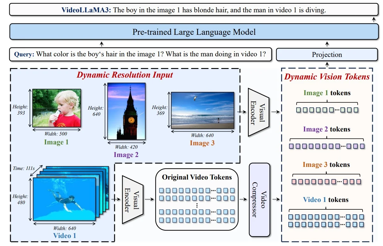
- Fidelity beyond grid heuristics Replace tiling/cropping with native-resolution tokenization to eliminate geometric distortion and preserve layout/text details in documents, charts, and high-resolution scenes [782, Sec. 3.1].
- Scalable token efficiency for longer videos Plan a clear visual budget within the LLM context and steer tokens toward motion and events via order-preserving sampling and content-aware pruning, so minutes of video remain tractable and temporal reasoning deepens instead of collapsing to coarse summaries [782, Sec. 2–3].
- One unified, instruction-friendly stream Represent images and videos in the same textualized format (newline/frame separators and simple Time: xxs stamps), enabling a single autoregressive interface to handle static VQA, multi-image comparison, long-video QA, and streaming dialogue [782, Sec. 3.3].
- Stable, staged learning First strengthen and align the vision prior on images, then add instruction following, and finally specialize for video; ablations indicate that adhering to this curriculum improves robustness and long-video performance compared to collapsing stages [782, Sec. 4.5].
Mechanisms chosen to meet these goals
- Any-resolution Vision Tokenization (AVT) Adapts the ViT to operate at native image/frame size and aspect (resolution-agnostic patch tokens), removing fixed crops or rigid tiling that inflate tokens or break layout [782, Sec. 3.1].
- Difference-aware Frame Pruning (DiffFP) Removes temporally redundant visual tokens before the LLM so long videos remain within context while preserving chronology; details follow in the next subsection [782, Sec. 2.2].
- Staged curriculum A four-stage progression (vision adaptation \(\rightarrow \) vision–language alignment \(\rightarrow \) multi-task SFT \(\rightarrow \) video-centric SFT) improves stability and transfer from strong image priors to temporal reasoning [782, Sec. 3]. Here, SFT means supervised fine-tuning on instruction-formatted input–output pairs (e.g., for the multi-task stage: image VQA, captioning, multi-image reasoning; for the video-centric stage: video QA, temporal grounding, streaming dialogue).
Scope: vision focus in V3 Unlike Video-LLaMA2, which explored audio-conditioned variants, Video-LLaMA3 is intentionally vision + language only: the paper and models do not introduce an audio branch [782]. This concentrates capacity and curated supervision on visual understanding, simplifies token budgeting for long clips, and aligns with benchmarks that evaluate visual comprehension (e.g., VideoMME without subtitles, MLVU, PerceptionTest, DocVQA, MathVista). The textualized interface remains compatible with future audio modules should they be interleaved later.
- Sharper spatial detail Native-resolution tokenization preserves small text and fine structure that uniform 3D aggregation in V2 tended to blur.
- Longer effective horizons Content-aware token savings target near-duplicate frames instead of uniformly compressing everything, enabling deeper temporal reasoning within a fixed LLM window.
Method
Pipeline at a glance Video-LLaMA3 uses a vision–centric pipeline that keeps native spatial detail while emitting tokens the LLM can read directly [782, Sec. 3]:
- Vision encoder A pretrained ViT-style backbone ingests images or video frames at their native aspect ratio/size and outputs per-patch features—no forced square crops or rigid tiling.
- Projector A small MLP maps encoder features to the LLM embedding dimension, yielding visual tokens that concatenate cleanly with text for unified autoregressive reasoning.
- Budgeted video packing Any-resolution Vision Tokenization (AVT) supplies per-frame, resolution-agnostic tokens; frames are serialized in time (optionally with simple Time: xxs tags) and, for long clips, a lightweight temporal compressor (DiffFP, described next) trims redundancy before the LLM.
This preserves fine structure (e.g., thin OCR strokes, small objects) and global layout while keeping token counts tractable for extended videos [782, Sec. 3].
Why a resolution-agnostic encoder Fixed-crop pipelines and grid-tiling “AnyRes” heuristics can distort aspect ratios, disrupt global layout, and bloat token counts on high-resolution or unusual-aspect inputs. Video-LLaMA3 replaces these heuristics with a genuinely resolution-agnostic encoder (via AVT) so every visual input—single images and all video frames—is processed at native size and aspect [782, Sec. 3.1]. The resulting token stream reflects actual visual content rather than an artificial tiling grid, which is crucial for documents, charts, and detail-heavy scenes, and it pairs naturally with later, change-aware pruning to extend the effective temporal horizon.
Any-resolution Vision Tokenization (AVT) AVT makes a ViT-based vision backbone resolution-agnostic, dynamically tokenizing images or video frames at their native sizes and aspect ratios to yield variable-length, LLM-ready tokens without cropping, resizing, or rigid tiling [782, Sec. 3.1]. The same procedure is applied to single images \(x\!\in \!\mathbb {R}^{C\times H\times W}\) and to each frame of a video \(x\!\in \!\mathbb {R}^{T\times C\times H\times W}\), with temporal serialization handled after spatial encoding.
- Native-resolution spatial patching (before tokenization). For each image or frame of size \(H{\times }W\), extract non-overlapping \(P{\times }P\) patches (stride \(P\)). This yields a grid \(H'=\lceil H/P\rceil \), \(W'=\lceil W/P\rceil \) and a sequence length \[ K \;=\; H' W' \;=\; \Big \lceil \frac {H}{P}\Big \rceil \!\cdot \! \Big \lceil \frac {W}{P}\Big \rceil \,. \] Each patch of shape \(C\!\times \!P\!\times \!P\) is flattened and linearly projected to a \(d\)-dimensional vector, producing a token sequence \(\mathbf {z}\in \mathbb {R}^{K\times d}\) that mirrors the native grid exactly. This “patchify \(\rightarrow \) embed” step fixes the geometry for positional encoding and avoids any rescaling or post-hoc interpolation artifacts.
-
Backbone adaptation to 2D-RoPE (spatial geometry). Replace the ViT’s fixed absolute positional table with 2D Rotary Position Embeddings (2D-RoPE) applied to queries/keys in every self-attention layer. Rotary encodings inject relative horizontal/vertical geometry via phase rotations, so the same encoder seamlessly handles arbitrary \(H'\!\times \!W'\) grids and aspect ratios without resizing or tiling [782, 225, Sec. 3.1].
-
Packing for the LLM (budgeted temporal serialization)
- Project to language space. A lightweight two-layer MLP with GELU maps each per-frame feature matrix \(\mathbf {f}_t \!\in \! \mathbb {R}^{K_t \times d}\) to \(\mathbf {v}_t \!\in \! \mathbb {R}^{K_t \times d_{\mbox{LLM}}}\).
- Images. For a single image, the visual tokens \(\mathbf {v} \!\in \! \mathbb {R}^{K \times d_{\mbox{LLM}}}\) are newline-separated and concatenated with text tokens, then fed to the LLM.
- Videos (chronological stream). For a clip with \(T\) frames, serialize \(\{\mathbf {v}_t\}_{t=1}^{T}\) in time to form one sequence \(\mathbf {V} \!\in \! \mathbb {R}^{(\sum _t K_t) \times d_{\mbox{LLM}}}\). Optionally prefix each frame block with a timestamp token (e.g., Time: xxs) and separate frames by commas to make temporal indices explicit.
- Context budgeting. Work within the LLM context window (e.g., total \(16{,}384\) tokens) by allocating a visual budget (e.g., \(\leq 10{,}240\) tokens) and reserving the remainder for text.
-
Order-preserving enforcement. If the visual stream exceeds the budget, apply simple, model-agnostic rules that keep chronology intact:
- Uniform frame sampling: increase the frame stride (e.g., decode at \(1\) fps and subsample to a target number of frames for short clips).
- Fixed \(2{\times }2\) spatial downsampling (post-encoder): apply \(2{\times }2\) pooling over the token grid to reduce each \(K_t\) while preserving aspect.
- Goal. Produce a well-ordered, budget-compliant visual sequence in which AVT preserves per-frame spatial fidelity; a content-aware pruning method for long videos is introduced next for additional savings [782, Sec. 3.1–3.2].
How 2D-RoPE encodes spatial relations 2D-RoPE lifts rotary embeddings from 1D to 2D image grids so self-attention depends on relative offsets \((\Delta u,\Delta v)\) instead of absolute indices [225, 782]. In Video-LLaMA3 this rotation acts per frame on spatial tokens; temporal order is handled later by serializing frames (optionally with Time: xxs) before they enter the LLM.
Attention recap. Take two patches at grid coordinates \((u,v)\) and \((u',v')\). Let \(x(u,v)\) and \(x(u',v')\) be their content embeddings. In one attention head, \[ q(u,v)=W_q\,x(u,v),\qquad k(u',v')=W_k\,x(u',v') . \] With 2D-RoPE, we rotate each query/key by an angle set by its own coordinates: \[ \tilde q(u,v)=R_{\phi (u,v)}\,q(u,v),\qquad \tilde k(u',v')=R_{\phi (u',v')}\,k(u',v') , \] where \(R_{\phi }\) is a tiny \(2{\times }2\) rotation applied per channel-pair (head dimension is even), and the angle is \[ \phi (u,v)=\theta _x\,u+\theta _y\,v \quad \mbox{(with a small bank of frequencies $\theta _x,\theta _y$ across pairs).} \] The attention score is the dot product \[ \big \langle \tilde q(u,v),\,\tilde k(u',v') \big \rangle , \] and the rotations make it depend only on the offsets \[ \Delta u = u-u',\qquad \Delta v = v-v' . \] Intuition: each token is “twisted” by an angle tied to its \((u,v)\). When two tokens interact, only the difference of those angles matters, so “one patch to the right” (e.g., \(\Delta u=-1,\Delta v=0\)) produces the same effect on any grid size. This is why 2D-RoPE is naturally resolution- and aspect-agnostic.
Why a new PE for arbitrary resolutions. Learned tables and absolute sinusoidals are tied to a specific lattice; when \(H'\!\times W'\) changes they need interpolation or reindexing and often drift off-distribution. RoPE encodes position as multiplicative rotations that compose inside the dot product, so the logit becomes a function of \((\Delta u,\Delta v)\) only. The notion “one patch to the right” is identical on \(14{\times }28\) and \(28{\times }56\) grids—no tables, no interpolation.
Setup and channel-pair rotations (encoding a patch at \((u,v)\)). After native-resolution patching, a frame yields a token grid with integer indices \((u,v)\), where \(u\!\in \!\{0,\dots ,H'-1\}\) and \(v\!\in \!\{0,\dots ,W'-1\}\). For the token at \((u,v)\), split \(q,k\!\in \!\mathbb {R}^{d}\) (even \(d\)) into \(d/2\) channel pairs \((x_{2i},x_{2i+1})\), each a tiny 2D plane we can rotate by \[ R_{\phi _i} \;=\; \begin {pmatrix} \cos \phi _i & -\sin \phi _i\\ \sin \phi _i & \phantom {-}\cos \phi _i \end {pmatrix}, \qquad \phi _i \;=\; \theta _x^{(i)}\,u \;+\; \theta _y^{(i)}\,v, \] where \(\{(\theta _x^{(i)},\theta _y^{(i)})\}_{i=1}^{d/2}\) is a frequency bank (typically geometric from coarse\(\!\to \!\)fine scales, fixed or lightly learned per head). Apply \(R_{\phi _i}\) to every pair of \(q\) and \(k\) to obtain the rotated vectors \(\tilde q,\tilde k\).
- Separable axial. Dedicate some pairs to rows (\(\phi _i=\theta _x^{(i)}u\)) and others to columns (\(\phi _i=\theta _y^{(i)}v\)).
- Mixed (diagonal-aware). Use \(\phi _i=\theta _x^{(i)}u+\theta _y^{(i)}v\) on all pairs to capture diagonals directly.
Which to use. Both realize the same relative property; mixed is often favored in vision because many structures (strokes, edges) are not axis-aligned.
Why pairs and where the frequencies come from. Treat \((x_{2i},x_{2i+1})\) as a complex coordinate \(x_{2i}+\mathrm {i}x_{2i+1}\). Multiplying by \(e^{\mathrm {i}\phi _i}\) (the rotation) preserves magnitude (content) while writing location into the angle. A geometric bank of \(\theta \)’s spreads sensitivity across spatial scales: low frequencies capture coarse layout, high frequencies capture fine detail (e.g., text strokes). Multi-head attention distributes these “frequency bins” across heads, so capacity is preserved.
Relativity in the logit (why resolution-agnostic). For tokens at \((u,v)\) and \((u',v')\) (write \(\Delta u{=}u{-}u'\), \(\Delta v{=}v{-}v'\)), \[ \big \langle \tilde q(u,v),\,\tilde k(u',v') \big \rangle \;=\; \sum _{i=1}^{d/2} \mathrm {Re}\!\Big [\,\alpha _i \, e^{\,\mathrm {i}\,(\theta _x^{(i)}\Delta u + \theta _y^{(i)}\Delta v)} \Big ], \] with coefficients \(\alpha _i\) determined by the unrotated content. The score is therefore a multi-scale, Fourier-like function of offsets \((\Delta u,\Delta v)\)—not of absolute \((u,v)\). The same \((\Delta u,\Delta v)\) produces the same phase gap across grids, enabling clean extrapolation to new resolutions and aspect ratios.
Efficient implementation. Because \(R_{\Theta }\) is block-diagonal, rotation reduces to pairwise elementwise ops: \[ \tilde q_{2i} = q_{2i}\cos \phi _i - q_{2i+1}\sin \phi _i,\qquad \tilde q_{2i+1} = q_{2i}\sin \phi _i + q_{2i+1}\cos \phi _i \] (and analogously for \(\tilde k\)). No dense matrix multiply is required.
Concrete intuition and example. Think of each channel pair as a compass needle. A patch at \((u,v)\) turns each needle by \(\phi _i=\theta _x^{(i)}u+\theta _y^{(i)}v\). Nearby patches turn needles by nearly the same angles (high overlap); distant patches turn them very differently (lower overlap).
For \(x\!\in \!\mathbb {R}^{3\times 224\times 448}\) with \(P{=}16\) (\(H'\!=\!14\), \(W'\!=\!28\)), the token at \((6,10)\) rotates by \(\phi _i=\theta _x^{(i)}\!\cdot \!6+\theta _y^{(i)}\!\cdot \!10\). Attending to \((7,10)\) introduces a horizontal phase gap proportional to \(\Delta u{=}{-}1\). Upscale to \(448{\times }896\) (\(28{\times }56\)) and the same neighbor relation yields the same phase gap—this is the core of resolution-agnostic behavior.
Why 2D-RoPE over absolute/sinusoidal PE (at a glance).
- Relative by construction. Offsets \((\Delta u,\Delta v)\) drive the logit, so no PE interpolation or reindexing is needed when \(H'\!\times W'\) changes.
- Table-free scaling. Angles are computed on the fly from integer coordinates; there are no size-specific lookup tables to retrain or resize.
- Multi-scale sensitivity. A frequency bank makes attention responsive to both coarse layout and fine detail while preserving a global receptive field.
Why time stays outside the vision PE. Video-LLaMA3 applies 2D-RoPE within each frame and leaves temporal order to the LLM by serializing frame tokens in time (optionally with simple Time: xxs tags) [782, Sec. 3.1–3.2]. This reuses strong image priors, keeps the vision stack lightweight (no 3D attention/PE), adapts naturally to variable frame counts under a token budget, and exploits the LLM’s strength on long sequences for temporal reasoning.
End-to-end position handling.
- Within a frame. Tokens lie on an integer grid \((u,v)\); 2D-RoPE rotates \(q/k\) using these coordinates, independent of flattening order.
- Across frames. Tokens are concatenated chronologically; timestamps provide explicit temporal indices for the LLM.
Differential Frame Pruner (DiffFP) Stacking per-frame tokens linearly with time produces long, redundant sequences dominated by static background regions. Video-LLaMA3 therefore introduces DiffFP, a simple, content-adaptive compressor that prunes patches with negligible temporal change while preserving key frames and motion regions [782, Sec. 3.2]. The procedure is two-stage:
(A) Uniform spatial downsampling (coarse bound). Each frame is first uniformly downsampled (e.g., \(2{\times }2\) bilinear) before patching/tokenization to place a coarse upper bound on per-frame tokens without destroying global context.
(B) Difference-aware patch pruning (fine, adaptive). Let a downsampled frame at time \(t\) be partitioned into \(H_p{\times }W_p\) patches, and let \(x_t(i,j)\in \mathbb {R}^{P{\times }P{\times }C}\) denote the pixel block (or an equivalent local descriptor used by the pruner) at patch \((i,j)\). DiffFP computes per-patch \(\ell _1\) differences to the previous frame and a frame-level change statistic: \[ d_t(i,j)\;=\;\bigl \|x_t(i,j)-x_{t-1}(i,j)\bigr \|_1,\qquad \Delta _t\;=\;\frac {1}{H_pW_p}\sum _{i=1}^{H_p}\sum _{j=1}^{W_p} d_t(i,j). \] With thresholds \(\tau _{\mbox{patch}}\) and \(\tau _{\mbox{frame}}\):
- Key-frame keep. If \(\Delta _t\ge \tau _{\mbox{frame}}\) (large global change), keep all patches of frame \(t\) to robustly capture scene cuts and large motions.
- Patch-wise keep. Otherwise, keep only patches with \(d_t(i,j)\ge \tau _{\mbox{patch}}\) and prune the rest, yielding a sparse set of motion patches for frame \(t\).
The resulting visual stream contains full key frames interleaved with sparse motion patches from intermediate frames, markedly shrinking the token budget while preserving the chronology and local dynamics needed for temporal reasoning. The pruned tokens are then concatenated (with text and, when present, additional modalities) and fed to the LLM for autoregressive generation.
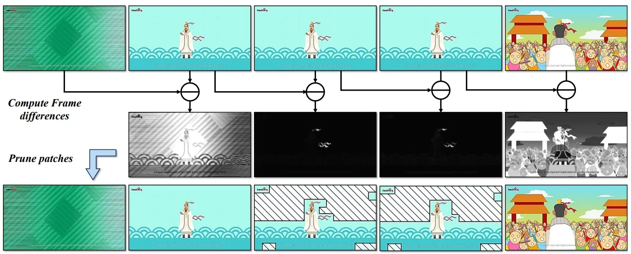
Data representations for multi-image, video, and streaming To unify static and temporal inputs in a single LLM interface, Video-LLaMA3 textualizes visual tokens with lightweight, literal delimiters that make structure explicit to the decoder [782, Sec. 3.3, Fig. 6]:
- Multi-image sequences. Visual token blocks for successive images are separated by the newline literal ∖n, and a final newline separates the vision block from the text prompt. This preserves per-image boundaries while enabling cross-image reasoning.
- Video sequences. Each frame’s tokens are prefixed by a timestamp literal Time: xxs and frames are comma-separated, e.g., Time: 0.0s [tokens], Time: 0.5s [tokens], …. A trailing ∖n then separates the visual stream from the text prompt. Timestamps provide explicit temporal anchors for ordering and duration.
- Streaming sequences. For long or live inputs, timestamped video token blocks and text turns are interleaved in one sequence (e.g., Time: 2.0s [tokens] USER:… ASSISTANT:…), enabling in-stream answers and multi-turn references to prior moments.
This delimiter-based serialization lets the LLM “read” images, videos, and streams as structured narratives, while AVT supplies faithful, resolution-agnostic tokens and DiffFP emphasizes informative changes over near-duplicate frames [782, Fig. 2, Fig. 6].
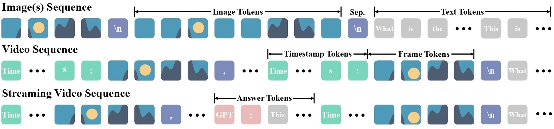
Architecture & Implementation Details
Backbone and projector Video-LLaMA3 couples a SigLIP-initialized ViT encoder with a lightweight two-layer MLP projector (GELU), a difference-aware video compressor (DiffFP), and a Qwen 2.5 family LLM for reasoning and generation [780, 782, 509]. Any-resolution Vision Tokenization (AVT) is realized by replacing the encoder’s learned absolute positional embeddings with 2D-RoPE and fine-tuning the vision stack on diverse images (scenes, documents, text-rich content). Compared to freezing the ViT (common in earlier pipelines), this adaptation is crucial: absolute PEs are tied to a fixed grid, whereas AVT demands resolution-agnostic geometry; fine-tuning lets attention heads and patch embeddings recalibrate to rotations, stabilizes scale/aspect extrapolation, and improves small-detail fidelity (OCR strokes, thin chart lines). Qwen 2.5 (e.g., 2B/7B) provides strong instruction following and long-context handling, while the shared vision stack keeps scaling cost moderate.
Training paradigm A four-stage curriculum builds a strong image prior first, then aligns and specializes for video [782]:
- Stage 1: Vision encoder adaptation. Swap absolute PEs for 2D-RoPE and fine-tune the SigLIP ViT and the projector on diverse images while keeping the LLM frozen. Intuition. Teach the encoder resolution-agnostic geometry (AVT) without language interference; freezing here would leave an absolute-PE mismatch that harms layout fidelity at new sizes/aspects.
- Stage 2: Vision–language alignment. Unfreeze encoder, projector, and LLM; jointly train on rich image–text data (including charts/regions) and mix in text-only samples. Intuition. Co-adapt vision features and the LLM so the language space learns to “read” variable-length, AVT tokens; text-only keeps linguistic fluency intact.
- Stage 3: Multi-task supervised fine-tuning (SFT). Instruction SFT over broad image tasks plus introductory video captioning; activate DiffFP to begin controlling video token counts. Intuition. Broaden skills and seed temporal competence while enforcing a practical token budget.
- Stage 4: Video-centric SFT. Focus on video QA, streaming, and temporal grounding with DiffFP active; continue mixing image-only and text-only data. Intuition. Specialize motion/event reasoning on top of the strong image prior, while guarding against catastrophic forgetting.
Where AVT and DiffFP plug in AVT. Enabled in Stage 1 by replacing absolute PEs with 2D-RoPE and fine-tuning the ViT + projector on images; thereafter, every image or frame is patchified at native aspect/size and encoded into resolution-agnostic tokens (no cropping/tiling). Why here. Early adaptation lets all later stages benefit from clean geometry and faithful layout.
DiffFP. Activated once video enters (Stages 3–4). Frames undergo fixed \(2{\times }2\) spatial downsampling post-encoder to bound per-frame token counts, then temporally redundant patches are pruned based on pixel-space \(\ell _1\) differences w.r.t. the previous frame (threshold \(\tau {\approx }0.1\) by default), preserving motion-bearing regions while cutting near-duplicates [782, Sec. 2.2]. Why here. Token budgeting is a delivery problem for the LLM context; doing it after spatial encoding keeps per-frame detail sharp and removes redundancy only when needed.
- SigLIP for strong visual priors. Sigmoid-based contrastive pretraining transfers well to text-heavy and diagrammatic images; fine-tuning with 2D-RoPE teaches resolution-agnostic geometry, improving small-detail fidelity over frozen backbones [780, 782].
- Qwen 2.5 for instruction reasoning. A modern LLM with long-context and multilingual strengths; a small projector maps vision features into the LLM space for stable alignment and scalable capacity [509].
- Video efficiency through DiffFP. Combine mild spatial downsampling with difference-aware patch pruning to fit long clips within a fixed context while emphasizing changes rather than static backgrounds [782].
- Stagewise curriculum for stability. Image \(\rightarrow \) multimodal \(\rightarrow \) video progressively aligns components, reduces optimization shock, preserves image/document skills, and yields better long-video transfer than collapsing stages [782].
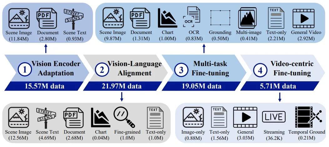
Experiments and Ablations
Benchmarks and headline performance Video-LLaMA3 is evaluated as a unified image+video MLLM and reports strong results across both video and image/math/doc tasks. For the 7B variant, representative accuracies include: MLVU (dev) 73.0%, VideoMME (w/o subtitles) 66.2%, PerceptionTest 72.8%, and MathVista (testmini) 67.1%. These trends align with the design goal: AVT preserves high-frequency spatial detail for documents/diagrams, while DiffFP focuses the budget on temporal changes for long clips.
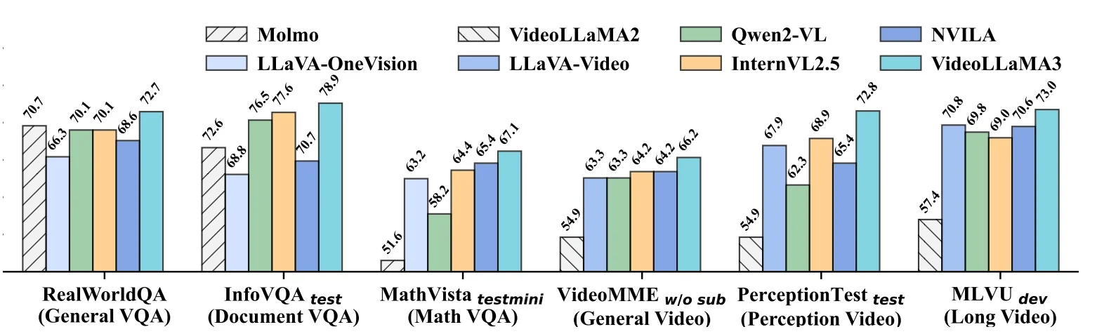
Effect of AVT and DiffFP Ablations separate the roles of Any-resolution Vision Tokenization (AVT) and Difference-aware Frame Pruning (DiffFP) [782, Sec. 3.1, Sec. 2.2, Sec. 4].
- AVT (2D-RoPE adaptation). Swapping absolute PEs for 2D-RoPE and ingesting images/frames at native aspect/size reduces geometric distortion and preserves small text/lines. The paper substantiates AVT with qualitative comparisons and aggregate benchmark gains on layout-sensitive tasks (documents, charts, diagrams) after the AVT stage, rather than a standalone numeric table isolating AVT alone [782, Fig. 2, Sec. 3.1, Sec. 4]. Intuition. AVT’s relative, table-free encoding makes “one-patch right” identical across grids, enabling clean transfer to unseen resolutions/aspects.
- DiffFP (video token efficiency). After mild per-frame \(2{\times }2\) downsampling to cap tokens, DiffFP prunes patches whose \(\ell _1\) pixel differences to the previous frame fall below a fixed threshold (default \(\tau {=}0.1\)) [782, Sec. 2.2]. The paper shows accuracy–token trade-off curves where substantial token reductions are achieved with negligible accuracy drops on long-video benchmarks under fixed context budgets (see [782, Fig. 4, Sec. 4]). Intuition. DiffFP targets static regions while retaining motion cues, reallocating budget to informative changes.
Relative to Video-LLaMA2 (uniform 3D aggregation), Video-LLaMA3 keeps spatial detail sharper and scales to longer videos via content-aware sparsification [782, 105, Sec. 2, Fig. 1]. Against similarly sized Qwen2-VL, it trends stronger on long-video and math/diagram reasoning in the authors’ composite chart, while approaching larger closed or semi-closed systems on several video tasks [782, Fig. 1]. Compared to image-first baselines (e.g., LLaVA-OneVision), Video-LLaMA3 maintains competitive document/multi-image reasoning and adds robust temporal understanding via its unified serialization interface [782, Sec. 3.3, Sec. 4].
Vision backbone ablation. Encoder studies support choosing a SigLIP-initialized ViT: after AVT adaptation and alignment, it yields strong text-aware features for OCR, charts, and fine-grained perception, outperforming alternatives on the authors’ image benchmarks [780, 782, Sec. 4.4]. Intuition. SigLIP’s contrastive pretraining plus 2D-RoPE adaptation gives a better prior for small, high-frequency structures than freezing an absolute-PE encoder.
Data curation and mixtures A staged, quality-over-quantity recipe builds image priors first, then specializes for video [782, Sec. 3.2, Tables 1–4].
- Vision Encoder Adaptation. 15.57M images spanning scenes, scene text/OCR, and documents to realize AVT and resolution-agnostic encoding.
- Vision–Language Alignment. 21.97M image–text pairs (incl. charts and fine-grained regions) plus text-only samples to retain language fluency.
- Multi-task Fine-tuning. 19.05M instruction-formatted image tasks plus general video captioning to seed temporal competence; DiffFP introduced for token control.
- Video-centric Fine-tuning. 5.71M video samples focused on video QA, streaming, and temporal grounding with DiffFP active.
Intuition. Image-first stages establish a strong, resolution-agnostic visual prior; later stages add instruction following and temporal specialization while DiffFP balances accuracy and context for long clips [782, Sec. 3.2, Sec. 4.5].
Limitations and Future Work
Long-context and token budgets. Although DiffFP reduces redundancy, extremely long videos still stress context limits; further hierarchical memory or event-level summarization could help.
Temporal precision and rare events Patch-level pruning with a fixed threshold may miss subtle, short-lived cues; adaptive thresholds or learned importance could improve recall on fine actions.
Data biases and domain transfer Vision-centric emphasis leverages curated image corpora; robustness to domain shifts (e.g., niche video domains or low-light/noisy streams) may require targeted data or adapters.
Toward Video-LLaMA4 Given Chapter Enrichment 24.9.2 highlighted STC for efficient motion aggregation, Video-LLaMA3 generalizes the idea with AVT+DiffFP for any-resolution and long-form efficiency. The next chapter on Qwen-VL families will revisit similar themes (high-res tokenization, streaming), and the subsequent Qwen3-VL hints at tighter multi-granular fusion and memory scheduling—directions also natural for the Video-LLaMA line.
Enrichment 24.9.5: Qwen-VL: Versatile Vision–Language Foundation
Motivation
Large multimodal systems frequently underperform on fine-grained visual skills (e.g., text reading, region grounding) and often lag behind proprietary models due to limited training scale and suboptimal optimization. The Qwen-VL paper targets these gaps by: (i) adding a position-aware visual receptor that compresses high-resolution visual features into a compact, LLM-friendly sequence; (ii) defining a concise input–output interface to unify images, text, and bounding-box strings; and (iii) designing a three-stage curriculum (pretraining, multi-task pretraining, supervised finetuning) over a multilingual, cleaned corpus [24].
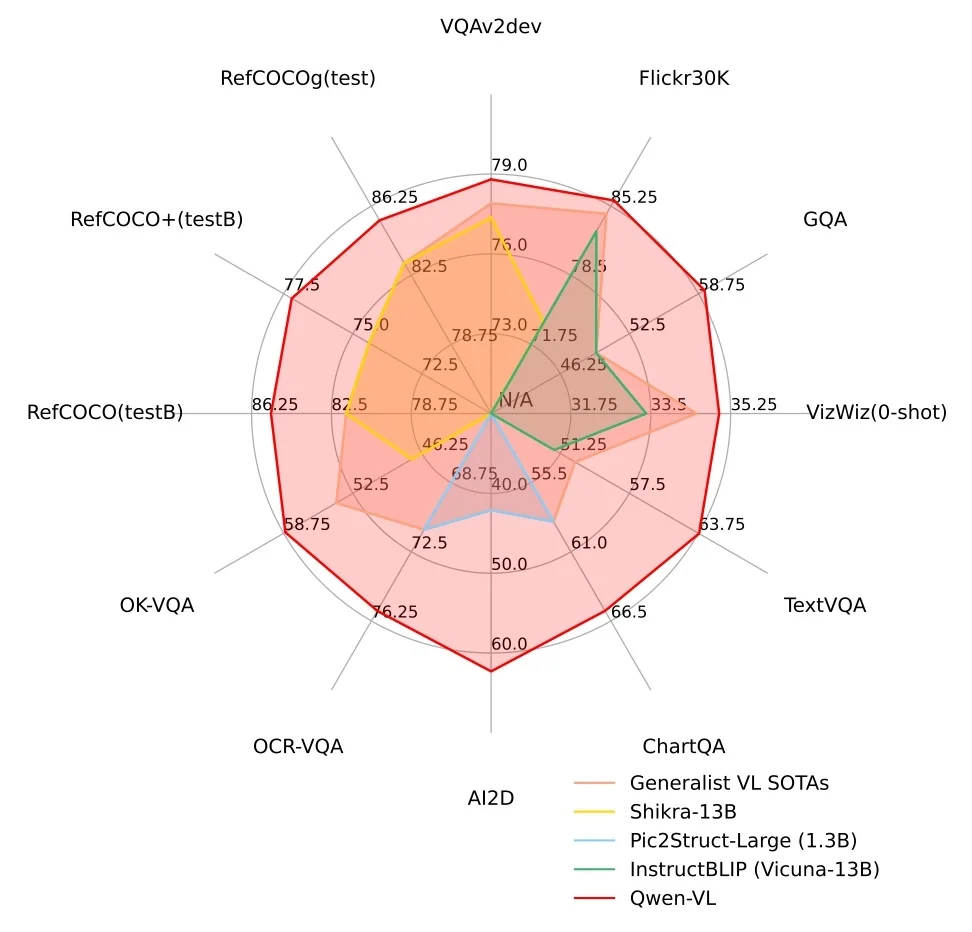
Reading the radar chart (intuition) Each spoke represents a benchmark (e.g., VQAv2, OK-VQA, TextVQA, OCR-VQA, ChartQA, RefCOCO). Larger area indicates stronger all-round performance. Qwen-VL’s polygon is notably expansive, reflecting broad generalization and especially strong text-rich understanding (TextVQA/OCR-VQA/ChartQA) relative to contemporary generalist baselines [24].
Method
Architecture (visual receptor + LLM) Qwen-VL integrates a high-capacity vision encoder, a lightweight position-aware adapter, and a large language model to enable unified multimodal reasoning [24].
- Vision encoder. A pretrained OpenCLIP ViT-bigG (patch stride \(P{=}14\)) extracts a sequence of patch features at the stage-specific input resolution, serving as robust perceptual tokens for downstream fusion [24].
- Position-aware VL adapter. A single cross-attention layer with \(M{=}256\) learnable query vectors compresses the variable-length image feature sequence into a fixed-length token set while injecting 2D absolute positional encodings into the attention to preserve spatial layout [24]. Relation to BLIP-2 Q-Former: both use learnable queries to distill visual features, but Qwen-VL adopts a single cross-attention layer (no stacked self/cross transformer blocks), prioritizing efficiency while retaining spatial fidelity via explicit 2D position signals.
- Large language model. A Qwen-7B LLM consumes the \(M\) adapter tokens interleaved with text to generate outputs, yielding a 9.6B-parameter system in total (Vision 1.9B, Adapter 0.08B, LLM 7.7B) [24, Table 1].
Input–output interface (tokenization and special tokens) Qwen-VL textualizes visual content and locations so the LLM can read, reason, and also output coordinates in plain text [24].
- Image tokens. The adapter’s \(M\) visual tokens are inserted as a contiguous block wrapped by <img> and </img> sentinels to clearly demarcate visual content from natural language tokens.
- Bounding boxes as text. Boxes are normalized to \([0,1000)\) and serialized as "(x_tl, y_tl), (x_br, y_br)"; <box>...</box> wrap the coordinate string, and <ref>...</ref> mark the referred phrase, enabling end-to-end grounding and box generation through standard autoregression.
Cross-attention compression (derivation and intuition) Let the ViT yield \(F\!\in \!\mathbb {R}^{N\times d_v}\) over \(N\) patches. The adapter maintains \(M\) learnable queries \(Z\!\in \!\mathbb {R}^{M\times d_q}\) with projections \[ Q \;=\; ZW_Q,\qquad K \;=\; FW_K,\qquad V \;=\; FW_V, \] and applies 2D absolute positional encodings to \((Q,K)\) before attention. The compressed tokens are \[ A \;=\; \mathrm {softmax}\!\Big (\frac {(Q{+}\mathrm {PE}_Q)(K{+}\mathrm {PE}_K)^\top }{\sqrt {d_h}}\Big ),\qquad H \;=\; A\,V \;\in \; \mathbb {R}^{M\times d_h}. \] Intuition. The learnable queries act like \(M\) content-and-position-aware “slots” that selectively pool salient regions while keeping geometry via 2D PEs, yielding a compact, spatially faithful summary for the LLM [24].
Training pipeline (three stages) Qwen-VL follows a staged curriculum to first align perception with language, then enrich tasks and resolution, and finally polish instruction following [24, Sec. 3].
- Stage 1: Pretraining (224\(\times \)224). Freeze the LLM and train the ViT and adapter on \(\sim \)1.4B cleaned image–text pairs (filtered from \(\sim \)5B) with next-token loss to establish basic vision–language alignment.
- Stage 2: Multi-task pretraining (448\(\times \)448). Unfreeze all modules and jointly train on captioning, VQA, grounding, referring grounding, grounded captioning, OCR, and pure-text autoregression (sequence length up to 2048), deepening high-resolution, fine-grained skills.
- Stage 3: Supervised finetuning. Freeze the ViT and finetune the adapter and LLM on curated multimodal dialogues that emphasize instruction following, multi-image conversation, and localization outputs.
Why this design Compared with feeding all ViT tokens directly, query-based cross-attention keeps the LLM context small and controllable while maintaining spatial detail through 2D position signals; compared with a deeper Q-Former stack, a single cross-attention layer reduces parameters and latency yet preserves the fine-grained cues needed for OCR and grounding thanks to high-resolution multi-task training [24].
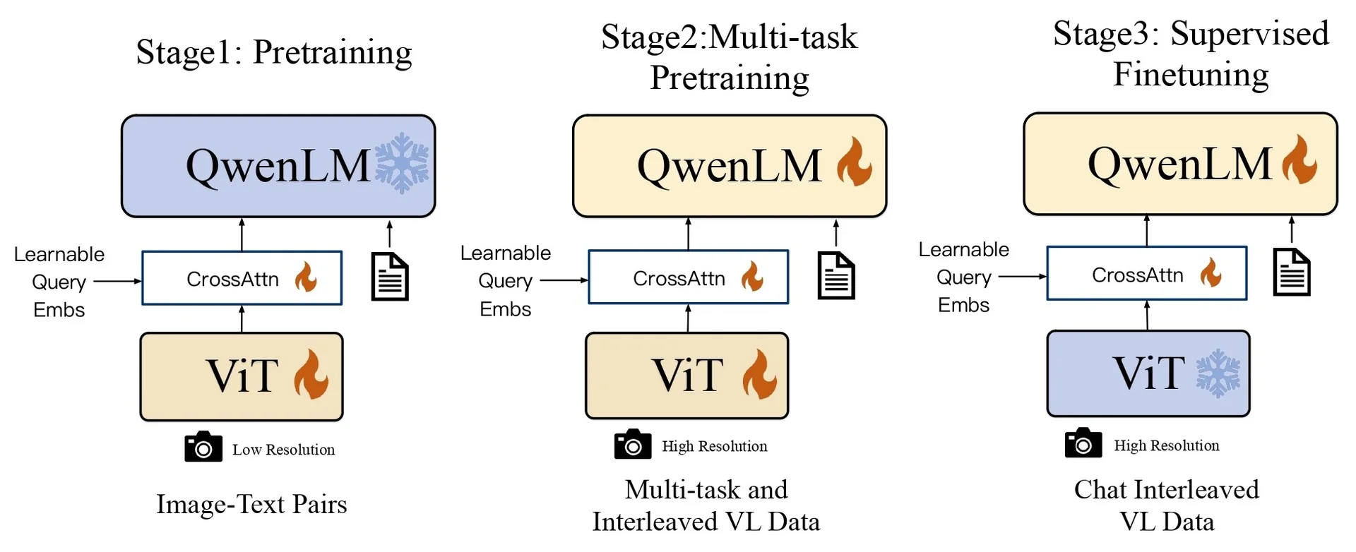
- Pretraining (scale and cleaning). Qwen-VL begins from roughly 5B image–text pairs and retains about 1.4B pairs (28%) after aggressive quality filtering, yielding a bilingual corpus. The retained pool draws primarily from LAION-en/LAION-COCO, DataComp, Coyo, CC12M/CC3M, SBU, and COCO Captions on the English side, plus LAION-zh (105M) and 220M in-house Chinese pairs, establishing broad coverage with cleaner supervision.
- Multi-task pretraining (what skills are taught). Around 69M supervised samples are used to teach diverse capabilities: captioning (19.7M), general VQA (3.6M), grounding (3.5M), referring expression comprehension and grounded captioning (8.7M each), and text-rich OCR understanding (24.8M), alongside 7.8M pure-text sequences to maintain language fluency. Representative sources include VQAv2, GQA, OK-VQA, GRIT, Visual Genome, RefCOCO/RefCOCO+/RefCOCOg, TextVQA, OCR-VQA, ChartQA, AI2D, SynthDoG (en/zh), and Common Crawl PDFs/HTML [24, Table 3].
- Design rationale. The data recipe is intentionally OCR-heavy for text reading, bilingual for cross-lingual robustness, and grounding-rich for localization; adding pure-text helps preserve the LLM’s linguistic priors while the vision–language tasks shape fine-grained multimodal reasoning [24, Sec. 3, Tables 2–3].
# Three-stage training of Qwen-VL (schematic)

# Init
vit = OpenCLIP_ViT_bigG()
llm = Qwen7B()                 # frozen in Stage 1
adapter = CrossAttnAdapter(    # 1-layer, M=256 learnable queries
    num_queries=256, use_2d_abs_pe=True
)

# Stage 1: Pretraining (224x224)
llm.freeze()
for batch in pretrain_loader(resolution=224):
    imgs, texts = batch
    F = vit(imgs)                      # patch features
    H = adapter.compress(F)            # M x d_h tokens
    tokens = wrap_img_tokens(H, texts)  # <img> ... </img> + text
    loss = autoregressive_ce(llm, tokens)
    update(vit, adapter)

# Stage 2: Multi-task pretraining (448x448)
llm.unfreeze()
vit.unfreeze()
for batch in multitask_loader(resolution=448, seq_len=2048):
    imgs, multimodal_tokens = batch    # interleaved image-text
    F = vit(imgs)
    H = adapter.compress(F)
    tokens = interleave(H, multimodal_tokens)
    loss = autoregressive_ce(llm, tokens)
    update(vit, adapter, llm)

# Stage 3: Supervised finetuning (instruction/chat)
vit.freeze()
llm.unfreeze()
for batch in sft_loader():
    imgs, chat_tokens = batch
    F = vit(imgs)
    H = adapter.compress(F)
    tokens = interleave(H, chat_tokens)  # includes boxes <box>...</box>
    loss = autoregressive_ce(llm, tokens)
    update(adapter, llm)
Architecture & Implementation Details
Backbone and adapter The ViT is initialized from OpenCLIP ViT-bigG; the adapter is a single cross-attention layer with trainable queries that compresses to \(M{=}256\) tokens, augmented with 2D absolute PEs in \((Q,K)\). The language backbone is Qwen-7B; Table 24.63 summarizes parameter counts [24].
Resolution and sequence length Images are \(224{\times }224\) in Stage 1 and \(448{\times }448\) in Stage 2; interleaved image–text sequences are packed to 2048 tokens during multi-task pretraining [24].
Special tokens and grounding format
To keep the interface simple and avoid overfull lines, Qwen-VL wraps visual
tokens between short sentinels <img> …</img> and expresses grounding with
<ref> …</ref> (text span) plus <box> …</box> (coordinates). Bounding boxes
are normalized to \([0,1000)\) and serialized compactly as (x_1,y_1),(x_2,y_2), which the
LLM reads and can also generate for localization [24].
Experiments and Ablations
Benchmarks and headline performance Qwen-VL targets image understanding with three representative result slices. Captioning/VQA: On Nocaps (0-shot) and VQAv2 it reports \(121.4\) CIDEr and \(79.5\%\), indicating robust vision \(\to \) language grounding [24, Table 4]. Text-rich VQA: On TextVQA it reaches \(63.8\%\), reflecting effective OCR + reasoning integration [24, Table 5]. Grounding: On RefCOCO test-A it attains \(92.26\%\), showcasing precise referring expression comprehension [24, Table 6]. The chat-tuned variant improves instruction following (e.g., SEED-Bench All \(58.2\)) and remains competitive on challenging zero-shot sets such as VizWiz (\(38.9\%\)) [24, Tables 4, 7].
What the ablations test The paper analyzes two design levers in the position-aware adapter + high-resolution regime: the number of learnable queries that compress ViT tokens, and the attention strategy used in the ViT at \(448{\times }448\) resolution.
- How many adapter queries (\(M\)) to use. The single cross-attention adapter pools dense ViT features into a fixed \(M\)-token summary. Appendix E.2 shows that accuracy rises as \(M\) grows and then saturates; \(M{=}256\) strikes the best speed/accuracy balance at \(448{\times }448\) and is adopted as default [24, Sec. 2.1, Appx. E.2]. Intuition: too few queries underfit fine detail; too many increase compute with diminishing returns.
- Global vs. window attention at high resolution. Appendix E.3 compares full (global) attention to windowed attention inside the ViT when moving from \(224{\times }224\) to \(448{\times }448\). Window attention trains more slowly (about \(2.5{\times }\) longer per step at \(448\) due to \(\sim 4{\times }\) tokens) and is sensitive to hyperparameters; more importantly, it reduces accuracy by nearly ten points on representative recognition/grounding targets in the authors’ setting, so global attention is preferred [24, Sec. 3.2, Appx. E.3]. Intuition: windowing saves FLOPs but weakens long-range interactions that help text reading and referring expression grounding.
How these results compare Relative to image-centric assistants (e.g., BLIP-2, InstructBLIP, Shikra), Qwen-VL reports stronger text-heavy understanding (e.g., TextVQA \(63.8\%\) vs. prior generalists at \(42{\sim }53\%\)) and competitive or better fine-grained grounding (e.g., RefCOCO test-A \(92.26\%\)) [24, Tables 4–6]. Direct score matching to video-focused systems (e.g., Video-LLaMA, LLaVA-Video) is not like-for-like because those benchmarks emphasize temporal reasoning; on image tasks, Qwen-VL generally exceeds LLaVA-style baselines reported in the Qwen-VL tables, while video models shine on long-video QA outside Qwen-VL’s scope [24, Fig. 1, Tables 4–7].
Design choices the ablations support The empirical findings consolidate three choices:
- Keep the adapter compact yet expressive. A single cross-attention layer with \(M{=}256\) learnable queries is sufficient for strong captioning/VQA and grounding while keeping end-to-end latency manageable [24, Sec. 2.1, Appx. E.2].
- Train at higher image resolution. Moving from \(224\) to \(448\) improves text reading and fine-grained perception; the authors therefore raise resolution in multi-task pretraining and keep the ViT frozen during SFT to preserve this fidelity [24, Sec. 3.2, Sec. 3.3].
- Prefer global attention at high resolution. Despite higher compute, global attention yields more stable training and clearly higher accuracy than windowed attention in the reported setting, which matters for OCR and grounding [24, Sec. 3.2, Appx. E.3].
Takeaways A compact, position-aware cross-attention adapter with \(M{=}256\) queries, coupled with higher-resolution multi-task training and global ViT attention, explains why Qwen-VL is strong on captioning/VQA (e.g., VQAv2 \(79.5\%\)), excels at text-centric understanding (e.g., TextVQA \(63.8\%\)), and remains competitive on grounding (e.g., RefCOCO test-A \(92.26\%\)) without task-specific heads [24, Tables 4–6].
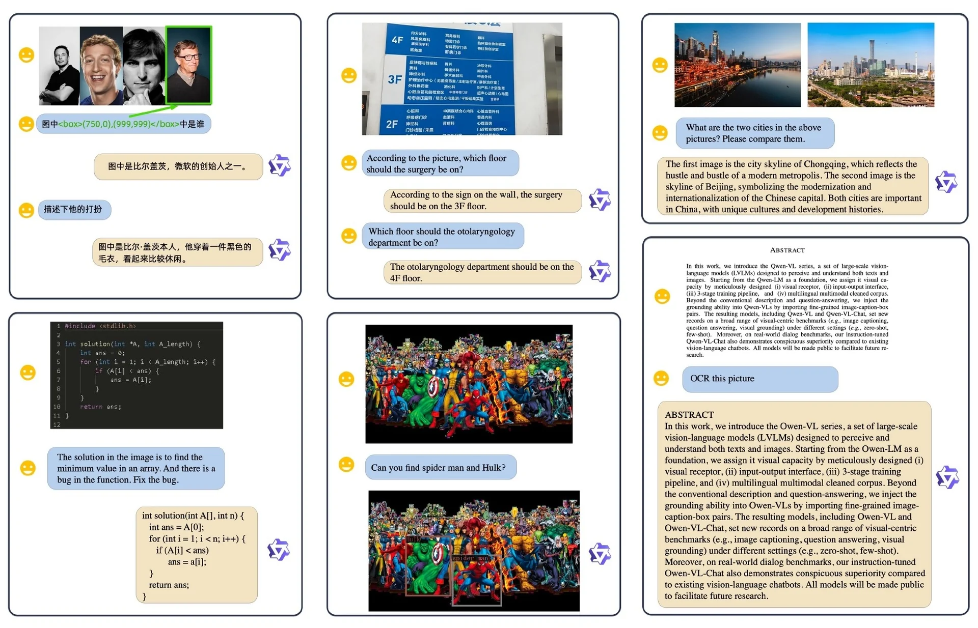
Qualitative capabilities Demonstrations include accurate referring-expression grounding with returned boxes, multilingual OCR with cross-lingual reasoning over signs and documents, multi-image comparative analyses, and structured content understanding such as code reading and correction, matching the interface design and high-resolution training [24].
Limitations and Future Work
While Qwen-VL establishes a strong generalist baseline with an efficient cross-attention adapter and a textualized grounding interface, several limitations in the 2023 design also outline a clear path for the next generation.
- Generalist–specialist gap. Qwen-VL emphasizes broad coverage across captioning, VQA, OCR-rich understanding, and grounding, yet single-task systems trained on narrowly curated data can remain ahead on their home benchmarks (e.g., chart understanding or dense scientific diagrams) [24, Sec. 5, Tables 4–6]. This motivates larger capacity and targeted mixtures to approach specialist quality without giving up generality.
- Compression bottleneck in the adapter. The single-layer, query-based adapter compresses variable-length ViT tokens to a fixed 256-token summary. This is compute-friendly, but can under-represent dense or highly cluttered scenes; the paper’s ablations select \(M{=}256\) as a speed/accuracy compromise rather than an upper bound [24, Sec. 2.1, Appx. E.2]. Future work can explore dynamic token budgets or multi-layer adapters that adapt capacity to content.
- Resolution and global context trade-offs. Moving from \(224{\times }224\) to \(448{\times }448\) improves text reading and fine detail, but also raises sequence length and training cost; windowed attention reduced accuracy in the reported setting, so the paper retained global attention with higher compute [24, Sec. 3.2, Appx. E.3]. This invites designs that keep long-range interactions while scaling to arbitrary resolution efficiently.
- Modality scope. Qwen-VL is image-centric; it does not natively model audio or video and relies on textualized coordinates for grounding [24, Sec. 2–3]. Extending to temporal and auditory modalities requires position schemes and tokenization that preserve time and synchronization in addition to space.
- Toward generation. The system focuses on understanding and localization rather than producing pixels or audio; closing the loop with vision or speech generation would require integrating diffusion/flow decoders or modular generators conditioned on the LLM [24, Sec. 5].
Bridge to Qwen2-VL These constraints foreshadow the priorities addressed by the successor model Qwen2-VL [689]: scaling capacity and data quality, introducing dynamic-resolution processing to better cover arbitrary sizes and dense layouts, and adding native video support with position schemes designed for multimodal time–space encoding. As the following summary of Qwen2-VL details, these changes directly target Qwen-VL’s compression and resolution trade-offs while broadening the modality scope.
Enrichment 24.9.6: Qwen2-VL: Dynamic Resolution Vision–Language Modeling
Motivation Many vision–language pipelines still resize inputs to a fixed canvas (e.g., \(224{\times }224\) or scale+pad), which can distort aspect ratios and suppress fine details; position encodings are often 1D or absolute 2D, which are not ideal for complex page layouts or temporal reasoning [335, 105, 782]. The Qwen-VL design (§Enrichment 24.9.4) alleviated these issues with a position-aware adapter and a textualized grounding interface, but still compressed vision to a fixed token budget at fixed training resolutions [24]. Qwen2-VL advances this line with two core ideas: naive dynamic resolution, which ingests images/documents at or near native sizes and produces a content-proportional number of visual tokens, and multimodal rotary position embedding (M-RoPE), which jointly encodes time, height, and width to unify text, images, and videos within one decoder [689]. Relative to the systems summarized in §Enrichment 24.7.2, §Enrichment 24.9.2, and §Enrichment 24.9.3, Qwen2-VL aims for a single native-resolution pipeline that scales across OCR, document understanding, and long-video reasoning, with 2B/7B/72B variants sharing the same vision stack.
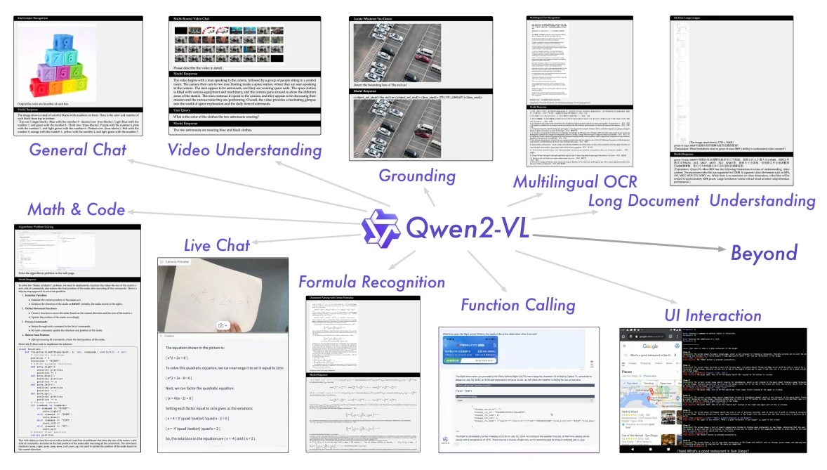
Method
- Naive dynamic resolution. Images are ingested at native resolution and extreme aspect ratios without global resize; token counts scale with content via a light 2\(\times \)2 token merger after the ViT to control sequence length.
- Multimodal RoPE (M-RoPE). Rotary position encodings are decomposed into temporal (\(t\)), height (\(h\)), and width (\(w\)) components, enabling consistent space–time indexing across text, images, and videos for attention.
- Unified image–video training. Images are treated as two identical frames (static \(t\)), while videos use true \(t\) with a shallow 3D stem; both pass through the same ViT and token merger before the LLM.
Naive dynamic resolution Let an input image \(\mathbf {x}\!\in \!\mathbb {R}^{H\times W\times C}\) be tokenized by a ViT with patch size \(p\), producing a grid \(\mathcal {G}\) of \(N{=}\lceil H/p\rceil \!\times \!\lceil W/p\rceil \) patch tokens \(F\!\in \!\mathbb {R}^{N\times d_v}\). Instead of resizing \(\mathbf {x}\) to a single fixed canvas, Qwen2-VL keeps the native grid and regulates length with a learnable \(2{\times }2\) token merger [689]. Concretely, for each non-overlapping \(2{\times }2\) neighborhood of tokens \(\{f_{i,j}\}_{(i,j)\in \{(2u,2v),(2u{+}1,2v),(2u,2v{+}1),(2u{+}1,2v{+}1)\}}\), the merger concatenates and projects \[ m_{u,v}\;=\;\phi \!\Big (\big [f_{2u,2v};\,f_{2u{+}1,2v};\,f_{2u,2v{+}1};\,f_{2u{+}1,2v{+}1}\big ]\,W_1\Big )\,W_2 \;\in \;\mathbb {R}^{d_v}, \] where \(W_1,W_2\) are linear layers and \(\phi \) is a pointwise nonlinearity. This reduces tokens by \(\approx 4{\times }\) while preserving local structure, yielding a content-proportional sequence length without distorting aspect ratios. When inputs are extremely large (e.g., tall documents or 4K scans), the same merger can be applied hierarchically (again on the merged grid) until a target budget is met, trading spatial detail for tractable context length in a controlled, locality-aware way. Multiple images are serialized by simple concatenation of their merged grids (each demarcated by vision sentinels) before interleaving with text in the decoder [689].
Videos \(\mathbf {V}\!\in \!\mathbb {R}^{T\times C\times H\times W}\) are handled frame-wise with the same mechanism. Let \(N_t\) be the per-frame tokens after patching and \(2{\times }2\) merging; the visual sequence length is \(\sum _{t=1}^{T}\!N_t\). To balance space and time under a global budget \(B_{\mathrm {vis}}\), Qwen2-VL uses simple policies such as: (i) per-frame merging depth chosen so \(N_t\!\le \!N_{\max }\); (ii) uniform or content-aware temporal subsampling (e.g., drop low-motion frames) if \(\sum _t N_t\!>\!B_{\mathrm {vis}}\); and (iii) capping the number of frames processed at native resolution while allowing coarser merging for the remainder [689]. Intuitively, this yields content-proportional tokens across images and videos: dense pages or keyframes retain more tokens, while redundant regions compress, preventing token overflow in long documents or long clips without uniform, detail-destroying downscales.
M-RoPE for space–time Rotary position embedding (RoPE) encodes relative offsets by rotating query/key channel pairs with a phase that depends on position. Standard 1D-RoPE uses a single index; Qwen2-VL generalizes this to three axes—time, height, width—via multimodal RoPE (M-RoPE) [689]. Each token is assigned a 3D ID \(\pi \!=\!(t,h,w)\), and the model allocates disjoint channel subspaces to the three axes. Writing a query head as \(\mathbf {q}\!\in \!\mathbb {R}^{d}\) with a partition \((\mathbf {q}^{(t)},\mathbf {q}^{(h)},\mathbf {q}^{(w)})\), M-RoPE applies axis-wise rotations \[ \widetilde {\mathbf {q}}^{(a)} \;=\; R^{(a)}(\pi _a)\,\mathbf {q}^{(a)},\quad R^{(a)}(\pi _a)\;=\;\bigoplus _{i=1}^{d_a/2} \begin {bmatrix} \cos \!\big (\theta ^{(a)}_i\,\pi _a\big ) & -\sin \!\big (\theta ^{(a)}_i\,\pi _a\big )\\[2pt] \sin \!\big (\theta ^{(a)}_i\,\pi _a\big ) & \phantom {-}\cos \!\big (\theta ^{(a)}_i\,\pi _a\big ) \end {bmatrix}, \quad a\in \{t,h,w\}, \] with analogous \(\widetilde {\mathbf {k}}^{(a)}\) for keys, where \(\{\theta ^{(a)}_i\}\) are geometric frequencies per axis and \(\oplus \) denotes block-diagonal composition. Concatenating the rotated subspaces gives \(\widetilde {\mathbf {q}},\widetilde {\mathbf {k}}\!\in \!\mathbb {R}^{d}\) used in attention. The inner product between two tokens with IDs \(\pi \) and \(\pi '\) then depends on their relative offsets \((\Delta t,\Delta h,\Delta w)\), which makes the attention scores equivariant to spatio-temporal translations. Qwen2-VL assigns IDs as follows: text tokens share a constant time index and a 1D progression along the width subspace (to preserve textual order); image tokens share a time index but use their \((h,w)\) grid locations; video tokens use frame order for \(t\) and per-frame \((h,w)\) for space [689].
Pseudo-code for dynamic resolution and M-RoPE
# Schematic pipeline: native-resolution vision, 2x2 token merger, M-RoPE assignment

def encode_image_or_video(frames, vit, merger2x2):
    """
    frames: list of HxW images (len=1 for image; >1 for video)
    vit: ViT with 2D-RoPE on spatial axes
    merger2x2: MLP that maps 4 patch tokens -> 1 token
    """
    visual_tokens = []
    for t, img in enumerate(frames):
        # 1) Native-resolution patching and ViT encoding (no global resize).
        F_hw = vit.patch_encode(img)                 # [H/p, W/p, C]
        # 2) 2x2 merger to control token count content-proportionally.
        F_merge = block_merge_2x2(F_hw)              # [H/(2p), W/(2p), C]
        # 3) Flatten to [N_t, C] and attach 3D position ids (t,h,w) for M-RoPE.
        T = flatten_with_ids(F_merge, t_axis=t)      # [(N_t, C), (ids_t,h,w)]
        visual_tokens.append(T)
        return concat(visual_tokens)                     # Variable-length visual sequence


def fuse_with_text(visual_tokens, text_tokens, llm):
    """
    Interleave markers and feed to LLM with multimodal RoPE activated on Q/K.
    """
    seq = [TOK.VISION_START] + visual_tokens + [TOK.VISION_END] + text_tokens
    return llm.generate(seq)
Why M-RoPE instead of 2D absolute encodings M-RoPE replaces the adapter’s 2D absolute position signals with a factorized, rotary scheme over time, height, and width, yielding a single spatio-temporal reference frame for text, images, video.
- Relative, resolution-agnostic geometry. Rotary phases encode relative \((\Delta h,\Delta w)\) offsets, improving layout transfer to unseen sizes and aspect ratios compared with absolute tables that require interpolation.
- Native temporal indexing. A dedicated temporal axis allows attention to condition on \(\Delta t\) jointly with \((\Delta h,\Delta w)\), enabling spatio-temporal reasoning for videos in a shared decoder space.
- Long-context stability. Using rotations tied to relative offsets avoids very large absolute indices, which empirically stabilizes extrapolation to long sequences.
Practical intuition.
- Video query. For “What happens after the ball crosses the line?”, attention can prioritize patches with small positive \(\Delta t\) near the line’s location in \((h,w)\), capturing immediate post-event dynamics.
- Document query. For “Read the footnote below the figure”, attention can target tokens with positive \(\Delta h\) under the referenced region within the same frame, preserving page geometry.
Scope. The paper focuses on text, image, and video; audio is not modeled and would require an additional axis or synchronized timestamping beyond this work [689].
Unified multimodal serialization
- Vision segment markers.
Visual tokens are delimited:
<|vision_start>and<|vision_end>to keep the interface LLM-native and avoid custom decoders [689]. - Grounding strings. Bounding boxes are normalized to \([0,1000)\) and serialized
compactly as
(x1,y1),(x2,y2); referred spans are output as plain text. The textual interface lets the LLM read and generate locations in one channel [689].
Architecture & Implementation Details
- Vision stack. The ViT employs 2D-RoPE and a shallow 3D stem for videos, followed by a 2\(\times \)2 token merger MLP to reduce sequence length with minimal local detail loss [689].
- LLM stack. The LLM is initialized from Qwen2 (2B/7B/72B) and trained to interleave visual and text tokens in one decoder stream with M-RoPE applied on attention [689].
- Training curriculum. The recipe follows Qwen-VL’s three stages: vision–language alignment at low cost, full multi-task image/video pretraining, and instruction tuning for chat, grounding, OCR, and tool use [689].
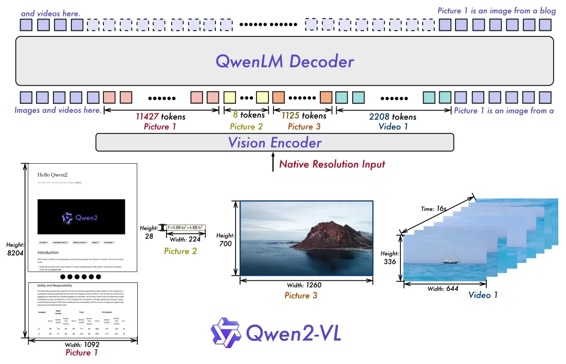
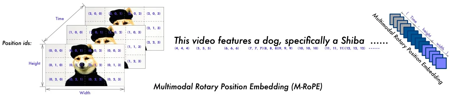
Experiments and Ablations
Benchmarks and headline performance Qwen2-VL shows very strong text–rich perception and competitive general reasoning, especially at 72B parameters [689]. On document/OCR style tasks, Qwen2-VL-72B attains DocVQA (test) \(96.5\) (GPT-4o \(92.8\), Claude-3.5 Sonnet \(95.2\)), TextVQA (val) \(85.5\), InfoVQA (test) \(84.5\), OCRBench \(877\), and RealWorldQA \(77.8\). On broad suites it is strong but not uniformly best: MMMU (val) \(64.5\) vs. GPT-4o \(69.1\) and Claude-3.5 \(68.3\); MMBench-EN (test) \(86.5\); MMEsum \(2482.7\) [689, Table 2]. The 7B variant offers a favorable cost–quality balance, e.g., TextVQA \(84.3\), OCRBench \(866\), RealWorldQA \(70.1\), MMMU (val) \(54.1\) [689, Table 2].
Video understanding Unified image–video training together with M-RoPE yields strong long–video results. Qwen2-VL-72B reports EgoSchema (test) \(77.9\) (GPT-4o \(72.2\)), MVBench \(73.6\), PerceptionTest (test) \(68.0\), and Video-MME \(71.2/77.8\) (w/o/w subtitles; GPT-4o \(71.9/77.2\)) [689, Table 4].
Grounding Referring expression comprehension scales with model size, approaching specialist detectors while retaining generality. Qwen2-VL-72B reaches RefCOCO (test-A) \(95.3\), RefCOCO+ (test-A) \(93.8\), and RefCOCOg (test) \(90.4\), improving on Qwen-VL and remaining close to specialist models such as ONE-PEACE, UNINEXT-H, and G-DINO-L [689, Table 6].
Multilingual OCR (internal) On an internal multilingual OCR suite, Qwen2-VL-72B surpasses GPT-4o on several languages (e.g., Korean \(94.5\) vs. \(87.8\), Japanese \(93.4\) vs. \(88.3\), French \(94.1\) vs. \(89.7\)), with a small shortfall on Arabic (\(70.7\) vs. \(75.9\)) [689, Table 3]. This reflects robust cross-lingual text reading while highlighting scripts that remain challenging.
Why dynamic resolution helps Ablations on Qwen2-VL-7B compare fixed image tokens to dynamic tokens that scale with content [689, Table 7]. Using a fixed budget of \(576\) image tokens yields InfoVQA (val) \(65.72\), RealWorldQA \(65.88\), and OCRBench \(828\), whereas dynamic resolution (avg. \(\sim 1924\) tokens for image content) attains \(75.89\), \(70.07\), and \(866\), respectively, while still consuming fewer tokens than the largest fixed settings. Accuracy is also robust across moderate fixed sizes (e.g., \(1600{\sim }3136\)), indicating that native-resolution packing plus the \(2{\times }2\) merger is an efficient default for text-heavy and dense layouts [689, Table 7].
Why M-RoPE matters Replacing 1D-RoPE with M-RoPE consistently improves video tasks and maintains or slightly improves image tasks [689, Table 8]. For example, PerceptionTest (test) rises from \(46.6\) to \(47.4\), NextQA from \(43.9\) to \(46.0\), and STAR from \(55.5\) to \(57.9\); on image benchmarks MathVista increases from \(39.2\) to \(43.4\) and MMBench from \(58.6\) to \(60.6\). These gains support the benefit of explicit \((t,h,w)\) encoding for unified space–time attention.
Length extrapolation With M-RoPE indexing, Qwen2-VL-72B sustains accuracy when the inference sequence length exceeds the \(16{,}384\) token training limit, remaining strong toward \(48\)K and beyond on Video-MME [689, Fig. 5].
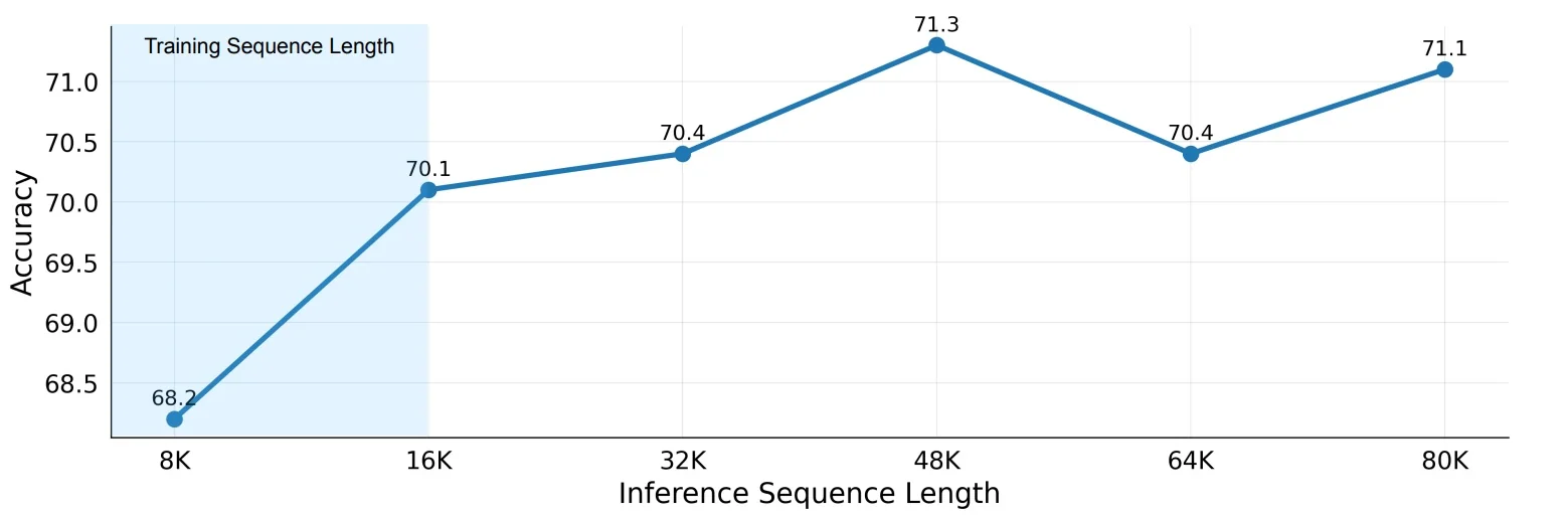
Resolution sensitivity
Varying min_pixels (i.e., upscaling small inputs before patching) shows that
moderate increases improve perceptual and text-rich tasks such as InfoVQA,
HallucinationBench, and OCRBench, with diminishing returns or slight drops at
extreme upscales [689, Fig. 4].
Scaling behavior and training curriculum Performance improves with model size across OCR, general VQA, video, and math, e.g., (2B \(\to \) 7B \(\to \) 72B) MVBench \(63.2 \to 67.0 \to 73.6\) and MathVista (testmini) \(43.0 \to 58.2 \to 70.5\) [689, Table 2, Fig. 6(a)]. The paper also analyzes the effect of increasing training tokens during the second pretraining stage for Qwen2-VL-7B: as the token count grows, most benchmarks improve smoothly (e.g., AI2D and InfoVQA), while some VQA scores fluctuate, consistent with task sensitivity to data mixtures [689, Fig. 6(b)]. Exact per-stage token totals are not disclosed; the reported trend supports allocating substantial budget to the multi-task, native-resolution stage to strengthen fine-grained perception and long-context use.
Limitations and Future Work
Qwen2-VL introduces native dynamic resolution, content-proportional visual tokens, and M-RoPE to unify images and video, yet several design trade-offs remain visible in the method and ablations [689]. The points below clarify where the current system can struggle and which directions the literature suggests are most promising.
- Resolution–efficiency trade-offs. Dynamic resolution with a \(2{\times }2\) token merger controls sequence length on most inputs, but extremely dense pages (e.g., long PDF scans, multi-column forms) or extreme aspect ratios can still yield very long visual sequences that push decoder context and memory [689, Table 2, Table 7]. Likely remedies include locality-aware ViT front-ends (adaptive strides or applying windows only where texture is high) and hierarchical merging that preserves fine detail selectively while keeping a coarse global map for long-range reasoning.
- Temporal grounding precision. M-RoPE provides a clean 3D positional scheme (time, height, width) but primarily encodes relative order, while downstream usage often requires absolute timestamps and robust handling of variable FPS [689, Table 4, Table 2, Fig. “Accuracy vs. Inference Sequence Length”]. Incorporating wall-clock alignment and FPS-aware sampling at the tokenizer level might improve fine-grained event localization over long videos without sacrificing the demonstrated length extrapolation.
- Structured extraction and precise geometry. The textual interface excels at free-form answers and box grounding, but applications needing strict schemas (e.g., JSON for invoices) or exact point/segment outputs can still trail specialist parsers and detectors; note that the paper’s grounding results chiefly report boxes on RefCOCO/+/g [689, Table 6]. Extending grounding beyond rectangles to points and polygons, and supervising format-faithful outputs (e.g., constrained decoding for tables/graphs), are natural follow-ups to close this gap.
- Long-context stability. Variable visual token counts improve fidelity yet also make runtime and memory less predictable for long, interleaved image+text+video sessions [689, Table 7, Fig. “Accuracy vs. Inference Sequence Length”]. A practical direction is to expose user-controllable token budgets and train learned token-pruning policies that down-weight redundant regions while preserving the rest.
- Hallucination control and attribution. Qwen2-VL improves robustness on perception and instruction tests, yet open-ended, multi-hop queries can still trigger visual or factual confabulations, as reflected by mixed movement on aggregate evaluations [689, Table 2]. Adding retrieval-augmented prompts for charts/docs and emitting visual evidence pointers (e.g., citing boxes or time spans used) can reduce ungrounded claims and aid auditing.
- Concise outlook: Qwen2.5-VL and Qwen3-VL. The Qwen2.5-VL report refines dynamic resolution handling with more efficient vision attention, introduces absolute-time indexing with dynamic FPS for video, extends grounding beyond boxes, and strengthens long-context efficiency [509]. Public descriptions of Qwen3-VL emphasize broader tool ecosystems and more stable long-horizon multimodal reasoning while retaining native-resolution fidelity; these directions align with the limitations outlined above.
Enrichment 24.10: Long-Context Modeling
Videos spanning minutes to hours demand mechanisms that scale beyond quadratic attention or strict autoregression. While recent VLLMs such as Video-LLaMA, the Qwen-VL family, and LLaVA-OneVision have pushed broad multimodal competence (instruction-following, OCR, grounding, AnyRes/dynamic-resolutions, multi-image interleaving), they typically rely on aggressive token compression, fixed or short temporal windows, or sparsified frame sampling. For truly long contexts—hour-long streams, movie-length narratives, live feeds—these heuristics alone are not enough; models must preserve salient details over time and offer compute that grows sub-quadratically with sequence length.
A timeline of approaches focused on long context.
- Memory-augmented transformers (2022). MeMViT [723] augments multiscale ViTs with segment-level external memory, pooling and reusing tokens across chunks. This turns naive “process each clip independently” into stateful inference, extending temporal support and improving accuracy without exploding computation.
- Streaming and state-space models (2023). Selective SSMs such as Mamba [196] maintain a compact recurrent state that is updated online as frames arrive, enabling linear-time inference in sequence length. This suits long or continuous video where latency and throughput matter more than full quadratic attention.
- Efficient long-video reasoning in VLLMs (2024). LongVLM [713] integrates memory caches, streaming updates, and sparse token selection into an LLM-centric pipeline, prioritizing serving-time constraints: it keeps the most informative spatiotemporal evidence, refreshes memory as new segments come in, and sustains coherent reasoning across long narratives.
- Blockwise/sparse attention for ultra-long sequences (first release - 2024). LWM [375] demonstrates Blockwise RingAttention to process million-token video–language contexts. Rather than compressing away detail, it restructures attention itself (blockwise, ring connectivity) so compute and memory scale to unprecedented lengths.
Enrichment 24.10.1: MeMViT: Memory-Augmented Multiscale ViTs
Motivation Many video backbones attain strong accuracy on short clips but become prohibitively expensive when naively scaling temporal support by feeding more frames to the model, causing quadratic growth in attention cost and ballooning GPU memory/runtime. The MeMViT paper proposes an alternative: process a long video online as a sequence of short clips and cache transformer keys/values as memory across iterations, so current queries can attend to a compact representation of the past with only marginal overhead [723]. Concretely, MeMViT reports temporal support up to \(30{\times }\) longer than baselines at just \(\sim \!4.5\%\) more compute, delivering higher accuracy under the same FLOPs envelope on AVA and other tasks.2
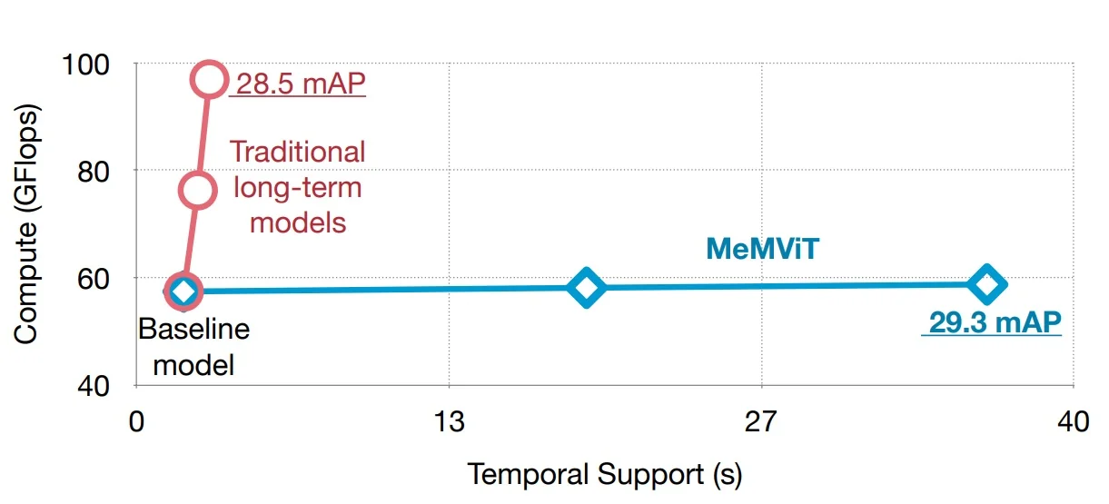
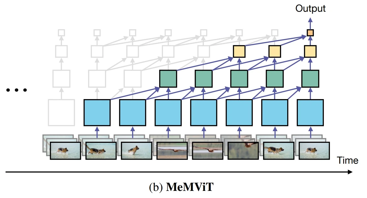
Preliminaries: ViT and MViT A standard transformer layer consumes a sequence of tokens \(X\!\in \!\mathbb {R}^{N\times d}\), projects to queries, keys, and values, \begin {equation} Q = XW_Q,\qquad K = XW_K,\qquad V = XW_V, \label {eq:memvit_linear} \end {equation} and applies scaled dot-product attention, \begin {equation} Z \;=\; \mathrm {Softmax}\!\left (\frac {QK^{\top }}{\sqrt {d}}\right )V,\qquad Z\in \mathbb {R}^{N\times d_{\mbox{out}}}. \label {eq:memvit_attn} \end {equation} ViT flattens image patches to form \(X\). For videos \(x\!\in \!\mathbb {R}^{T\times C\times H\times W}\), a tubelet embedding with tube size \((t_p\!\times \!p\!\times \!p)\) yields \[ N_0 \;=\; \frac {T}{t_p}\cdot \frac {H}{p}\cdot \frac {W}{p},\qquad Z_0\in \mathbb {R}^{N_0\times d_0}, \] so naively attending over all tokens scales quadratically in \(N_0\), which grows quickly with \(T\), \(H\), and \(W\).
MViT: multiscale hierarchy + pooling attention. Multiscale ViT (MViT) addresses video scale by borrowing two CNN-style principles [152, 354]:
- Multi-stage pyramid. The model is organized into stages \(s=1,\dots ,S\). Each stage reduces spatiotemporal resolution (token count) while increasing channel capacity, producing a sequence \(Z_s\!\in \!\mathbb {R}^{N_s\times d_s}\) with \(N_{s+1}\!<\!N_s\) and \(d_{s+1}\!>\!d_s\). This yields large receptive fields and efficient compute at deeper layers, analogous to CNN feature pyramids.
- Pooling attention. Inside a stage, attention cost is reduced by pooling along \((t,h,w)\) before forming \(Q,K,V\) (“pool-then-attend”), or equivalently pooling intermediate representations that generate \(Q,K,V\) (“pooling attention”). This shrinks the token dimension over which attention operates, lowering the quadratic factor in \(N_s\) without discarding channel information relevant for recognition.
Concretely, let a stage-\(s\) block view its input as a 4D tensor \(X_s\!\in \!\mathbb {R}^{T_s\times H_s\times W_s\times d_s}\) (with \(N_s\!=\!T_sH_sW_s\) after flattening). The improved MViT variant adopted by MeMViT applies lightweight spatiotemporal pooling before linear projections [354]: \begin {equation} \bar Q_s = P_Q(X_s),\quad \bar K_s = P_K(X_s),\quad \bar V_s = P_V(X_s),\qquad Q_s = \bar Q_s W_Q,\; K_s = \bar K_s W_K,\; V_s = \bar V_s W_V, \label {eq:memvit_pool_then_linear} \end {equation} where \(P_{\{\cdot \}}\) are strided average-pooling (or equivalent) operators over \((T_s,H_s,W_s)\) that reduce token count from \(N_s\) to \(\bar N_s\!\ll \!N_s\) while preserving channels \(d_s\). Attention then runs on \((\bar N_s\times \bar N_s)\) rather than \((N_s\times N_s)\). Intuitively, early stages keep many fine-grained tokens and small \(d_s\) for local motion/texture; later stages operate on few tokens with large \(d_s\) for global semantics. This pyramidal design provides a compute-efficient path to long-range spatiotemporal context and forms the backbone on which MeMViT attaches its memory mechanism.
Method: Memory Attention and Hierarchical Caching Clip-wise online attention with a rolling \(K/V\) cache (flattening & multi-head shapes). Given a video \(x\!\in \!\mathbb {R}^{T\times C\times H\times W}\), MeMViT streams it as clips \(x^{(t)}\!\in \!\mathbb {R}^{\tau \times C\times H\times W}\) in order \(t{=}1,2,\dots \) [723, Sec. 4.1]. Each clip is tubelet-tokenized and passed through an MViT stage that first pools then projects (Eq. (24.36)). After pooling along \((t,h,w)\), the stage-\(s\) activations have grid shape \[ \tilde Q^{(t)},\tilde K^{(t)},\tilde V^{(t)}\in \mathbb {R}^{T_p\times H_p\times W_p\times d_s}, \] which are flattened (e.g., \(t\)-major, then row-major over \((h,w)\)) to sequences \[ \bar N_s \;=\; T_pH_pW_p,\qquad \bar Q^{(t)},\bar K^{(t)},\bar V^{(t)}\in \mathbb {R}^{\bar N_s\times d_s}. \] Flattening is valid because self-attention is permutation-equivariant; a geometry-respecting rasterization preserves locality.
Multi-head attention notation and weight shapes. Let the model width at stage \(s\) be \(d_s\) and the number of heads be \(h\). The per-head width is \(d_h\) with \[ d_s \;=\; h\,d_h. \] There are two equivalent ways to write the projection matrices:
- Packed (all heads at once): \(W_Q,W_K,W_V\in \mathbb {R}^{d_s\times d_s}\) map \(d_s\!\to \!d_s\); outputs are then reshaped to \((h,\cdot ,d_h)\).
- Per-head view (clearer for shapes): for each head \(r\!\in \!\{1,\dots ,h\}\), \(W_Q^{(r)},W_K^{(r)},W_V^{(r)}\in \mathbb {R}^{d_s\times d_h}\) map \(d_s\!\to \!d_h\) and are applied in parallel, then concatenated along the last dim to recover \(d_s\).
Both views are identical because \(h\,d_h\!=\!d_s\). After attention, the \(h\) head outputs (each \(d_h\)) are concatenated to \(\mathbb {R}^{\bar N_s\times (h d_h)}{=}\mathbb {R}^{\bar N_s\times d_s}\) and mixed by the standard output projection \[ W_O \in \mathbb {R}^{d_s\times d_s}, \] which linearly combines head channels back into the stage width.
Current-step projections (with shapes). Using the per-head view for clarity, for head \(r\): \[ Q_r^{(t)}=\bar Q^{(t)}W_Q^{(r)}\in \mathbb {R}^{\bar N_s\times d_h},\;\; K_{r,\mbox{cur}}^{(t)}=\bar K^{(t)}W_K^{(r)}\in \mathbb {R}^{\bar N_s\times d_h},\;\; V_{r,\mbox{cur}}^{(t)}=\bar V^{(t)}W_V^{(r)}\in \mathbb {R}^{\bar N_s\times d_h}. \]
Rolling \(K/V\) cache. MeMViT augments the current keys/values with a FIFO cache from the previous \(M\) clips, stopping gradients into cached steps (read-only memory) [723, Sec. 4.1]: \begin {align} \bar K^{(t)} \;:=\; \big [\,\mathrm {sg}(\bar K^{(t-M)}),\ldots ,\mathrm {sg}(\bar K^{(t-1)}),\bar K^{(t)}\,\big ]\in \mathbb {R}^{(\bar N_s{+}N_m)\times d_s}, \label {eq:memvit_basic_K}\\ \bar V^{(t)} \;:=\; \big [\,\mathrm {sg}(\bar V^{(t-M)}),\ldots ,\mathrm {sg}(\bar V^{(t-1)}),\bar V^{(t)}\,\big ]\in \mathbb {R}^{(\bar N_s{+}N_m)\times d_s}, \label {eq:memvit_basic_V} \end {align}
where \(N_m\) is the number of cached (flattened) tokens. Concatenation is along the token axis; the last dimension remains \(d_s\), so the same \(W_K^{(r)},W_V^{(r)}\) apply to both current and cached rows: \[ K_r^{(t)}=\bar K^{(t)}W_K^{(r)}\in \mathbb {R}^{(\bar N_s{+}N_m)\times d_h},\qquad V_r^{(t)}=\bar V^{(t)}W_V^{(r)}\in \mathbb {R}^{(\bar N_s{+}N_m)\times d_h}. \] Per head, attention is \[ Z_r^{(t)}=\mathrm {Softmax}\!\Big (\tfrac {Q_r^{(t)}(K_r^{(t)})^\top }{\sqrt {d_h}}\Big )\,V_r^{(t)}\in \mathbb {R}^{\bar N_s\times d_h}, \] then \(Z^{(t)}=[Z_1^{(t)}\|\cdots \|Z_h^{(t)}]\in \mathbb {R}^{\bar N_s\times d_s}\) and \(Z^{(t)}W_O\) restores stage width.
Why the complexity is linear in cache size. Only the current \(\bar N_s\) tokens emit queries; cached tokens supply keys/values but no queries. Per head, the cost of forming the attention logits is \(\mathcal {O}(\bar N_s(\bar N_s{+}N_m)d_h)\) (matrix multiply \(Q_r^{(t)}[\,\bar N_s\times d_h\,]\) by \((K_r^{(t)})^\top [\,d_h\times (\bar N_s{+}N_m)\,]\)), which scales linearly with \(N_m\) and avoids the \(\mathcal {O}((\bar N_s{+}N_m)^2)\) blow-up of treating all tokens (past+present) as queries.
Keeping \(N_m\) small via learnable compression. Cached keys/values are downsampled by spatiotemporal pooling \(f_K,f_V\) that preserve channel width \(d_s\) but reduce token count by a factor such as \(4{\times }2{\times }2\) over \((T,H,W)\) [723, Sec. 4.2]. If the current stage has \(\bar N_s\) tokens, each past clip contributes \(\hat N_{m,s}=\bar N_s/16\) compressed tokens. After concatenation, augmented tensors have shape \((\bar N_s{+}M\hat N_{m,s})\times d_s\), and per head \[ (\bar N_s{+}M\hat N_{m,s})\times d_s \xrightarrow {\;W_{K/V}^{(r)}\in \mathbb {R}^{d_s\times d_h}\;} (\bar N_s{+}M\hat N_{m,s})\times d_h, \] which matches the current-step projections. Because cached tokens supply only \(K/V\) and are gradient-stopped, per-head complexity is \(\mathcal {O}\!\big (\bar N_s(\bar N_s{+}M\hat N_{m,s})\big )\) (linear in cache size), not \(\mathcal {O}\!\big ((\bar N_s{+}M\hat N_{m,s})^2\big )\).
How the rolling cache is used and updated (numerical example). For \(T{=}128\) processed as \(\tau {=}16\)-frame clips with tubelets \((t_p{=}2,p{=}16)\) at \(224{\times }224\), the first stage sees \(\bar N_s=\tfrac {16}{2}\cdot \tfrac {224}{16}\cdot \tfrac {224}{16}=1568\) tokens for \(x^{(1)}\) and attends within the clip (empty cache). After attention, that layer stores a compressed summary \((\hat K,\hat V)\) for future steps. At \(t{=}2\), queries from \(x^{(2)}\) (\(\bar N_s{=}1568\)) attend to the concatenation of cached \((\hat K,\hat V)\) from \(x^{(1)}\) and current \((\bar K,\bar V)\) from \(x^{(2)}\). The cache acts as a read-only KV store (stop-gradient), so only the present \(\bar N_s\) queries are formed; past tokens do not query each other. The same mechanism applies at deeper MViT stages where \(\bar N_s\) is smaller, so the relative overhead further shrinks while temporal receptive field grows hierarchically [723, Sec. 4.1].
Pipelined memory compression (constant-time update). Instead of recompressing all cached clips every iteration, MeMViT compresses only the freshest uncompressed step and reuses older compressed entries: \begin {align} \bar K^{(t)} \;:=\; \big [\, \hat K^{(t{-}M)},\,\ldots ,\,\hat K^{(t{-}2)},\, f_K\!\big (\mathrm {sg}(\bar K^{(t{-}1)})\big ),\, \bar K^{(t)} \,\big ], \qquad \hat K^{(t')} \;=\; \mathrm {sg}\!\big (f_K(\bar K^{(t')})\big ), \label {eq:memvit_pipeline} \end {align}
and analogously for values. With a \(4{\times }2{\times }2\) pool, each past clip contributes \(1568/16=98\) tokens; for \(M{=}2\), the current attention sees \(1568{+}2\!\cdot \!98=1764\) keys/values, i.e., \(\sim \!12\%\) overhead for a longer per-layer temporal horizon [723, Fig. 4, Table 1(b)]. Intuitively, the pipeline is a conveyor belt: each step “seals” the previous clip into a compact, trainable summary and shifts older summaries forward without recompression, keeping compute and memory near-constant over time.
Where memory is attached (hierarchical receptive fields). Memory augmentation may be applied to all layers or a subset. Empirically, alternating memory-augmented and standard attention layers often yields the best accuracy/efficiency trade-off [723, Table 1(c)]. Shallow layers (large \(\bar N\)) store fine motion/texture cues; deep layers (small \(\bar N\)) store semantic summaries. This layered placement grows the temporal receptive field with depth while the marginal memory overhead shrinks, enabling long-term modeling (tens of seconds) at modest extra FLOPs compared with the same MViT backbone without memory [723, Sec. 4.1–4.2].
Algorithmic sketch (from the paper)
# Algorithm 1 (from Wu et al., 2022): MeMViT attention (PyTorch-like)
class MeMViTAttention():
    # pool_q, pool_k, pool_v: pooling layers
    # lin_q, lin_k, lin_v: linear layers
    # f_k, f_v: compression modules
    def __init__(self, max_mem):
        self.m_k = []  # cached memory keys
        self.m_v = []  # cached memory values
        self.max_mem = max_mem

    def forward(self, x):
        # compute pooled Q, K, V
        q, k, v = pool_q(x), pool_k(x), pool_v(x)

        # compress only the immediate previous memory (pipelined)
        cm_k = f_k(self.m_k[-1]) if len(self.m_k) > 0 else None
        cm_v = f_v(self.m_v[-1]) if len(self.m_v) > 0 else None

        # concatenate (older compressed ..., newly compressed prev, current)
        aug_k = cat(self.m_k[:-1] + ([cm_k] if cm_k is not None else []) + [k])
        aug_v = cat(self.m_v[:-1] + ([cm_v] if cm_v is not None else []) + [v])

        # attention
        z = attn(lin_q(q), lin_k(aug_k), lin_v(aug_v))

        # update caches: replace prev with its compressed copy
        if len(self.m_k) > 0:
            self.m_k[-1] = cm_k.detach()
            self.m_v[-1] = cm_v.detach()

        # append current uncompressed memory for next iteration
        self.m_k.append(k.detach())
        self.m_v.append(v.detach())

        # enforce memory length
        if len(self.m_k) > self.max_mem:
            self.m_k.pop(0)
            self.m_v.pop(0)
        return z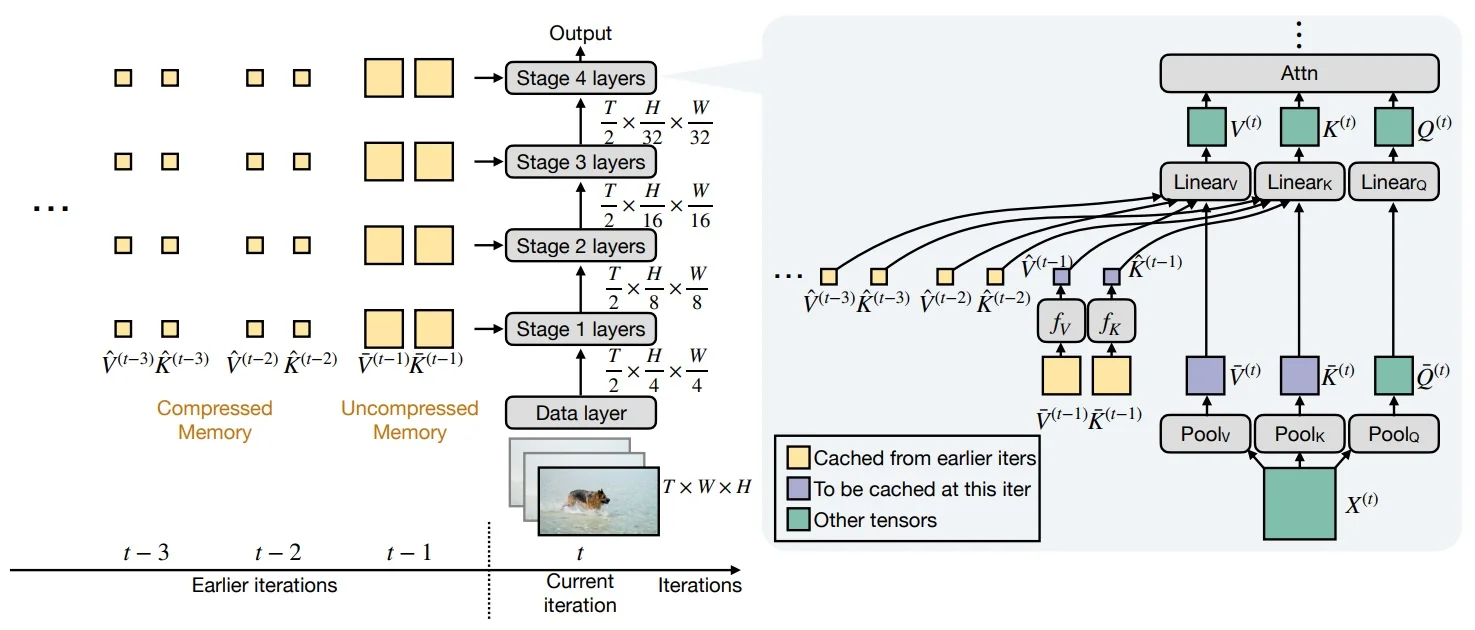
Architecture & Implementation Details
Backbone and stages MeMViT instantiates the memory augmentation on top of MViT [152, 354], typically with an MViT-B backbone (16 layers) and 16-frame input clips at stride 4 (“\(16{\times }4\)”). The model proceeds through multiple stages with token downsampling (spatiotemporal pooling) between stages; memory augmentation can be placed at all or a subset of attention layers.3
Data loading and training During both training and inference, videos are read sequentially as clips to mimic streaming: the implementation concatenates all videos and iterates through them in order. At a video boundary—when the next clip belongs to a new video—any memory carried over from the previous video is masked to zero so that unrelated context does not leak across videos. Default training follows standard MViT settings: backbone MViT-B (16 layers) with \(16{\times }4\) clips, Kinetics-400 pre-training (unless stated), AVA fine-tuning for 30 epochs with SGD (batch 128), random horizontal flips and \(224^2\) crops; FLOPs are reported at \(224^2\) input resolution [723, Sec. 5].
Experiments and Ablations
Scaling strategies Relative to the common baseline that increases the number of input frames \(T\), MeMViT attains much longer temporal support with near–flat increases in training/inference GPU memory, runtime, and FLOPs, while achieving higher mAP at comparable cost [723, Fig. 3]. The below figure visualizes this trade–off: simply scaling \(T\) rapidly exhausts memory and compute, whereas MeMViT’s hierarchical rolling cache sustains long–range context at modest cost.
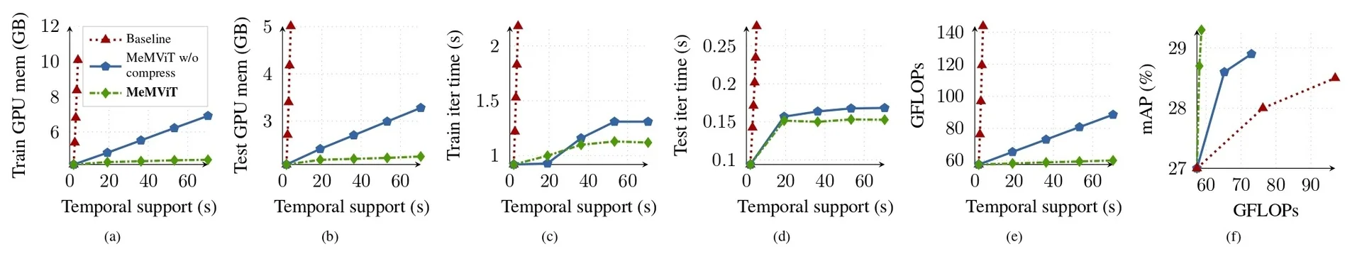
Ablations: how memory is used On AVA [197] with an MViT-B (\(16{\times }4\)) backbone [354] pretrained on Kinetics-400, MeMViT improves from \(27.0\) to \(29.3\) mAP at a small FLOPs increase (\(57.4{\to }58.7\)G) [723, Table 3]. Layer–wise memory length \(M\) shows the best trade–off at \(M{=}2\): \(M{=}1\) (effective \(8{\times }\) receptive field) yields \(28.7\) mAP, \(M{=}2\) (\(16{\times }\)) reaches \(29.3\), and overly long \(M{=}4\) (\(32{\times }\)) saturates to \(28.8\) [723, Table 1(a)]. Placing memory in about half of the transformer layers achieves the peak \(29.3\) mAP while reducing compute versus augmenting all layers [723, Table 1(c)]. For compression, aggressive temporal downsampling is more tolerable than spatial: e.g., a \(4{\times }2{\times }2\) (time:height:width) factor reaches \(29.3\) mAP at \(\approx 58.7\)G FLOPs, whereas equally aggressive spatial compression harms accuracy [723, Table 1(b)].
Pipeline vs. naive compression The pipelined strategy—compressing only the freshest cached step while reusing earlier compressed memory—reduces training GPU memory and iteration time compared with recompressing all cached steps each iteration, without sacrificing accuracy [723, Fig. 4]. Figure 24.120 highlights the improved scaling behavior.
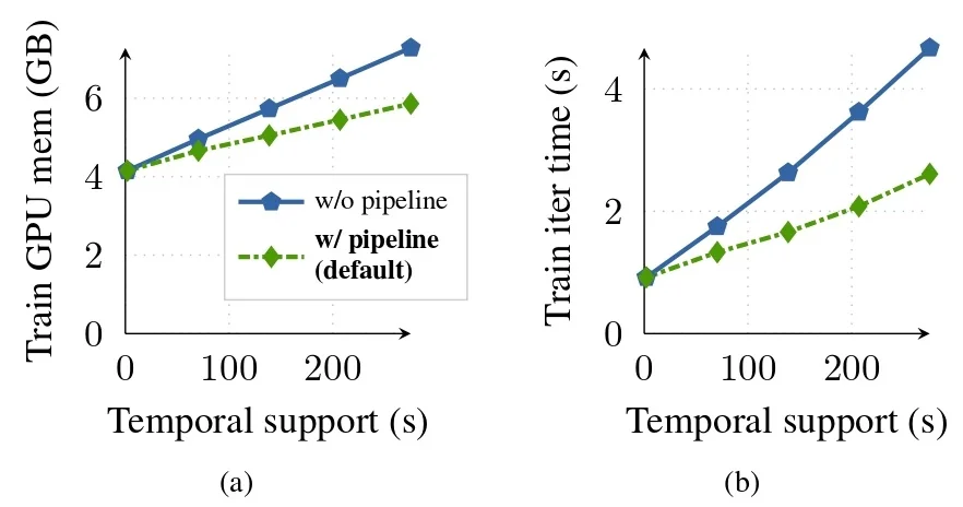
Generalization across backbones and datasets Improvements persist with larger backbones and stronger pretraining. With MViT-24 (\(32{\times }3\)), MeMViT improves AVA mAP from \(32.5\) to \(34.4\) under Kinetics-700 pretraining, at similar compute (\(204.4{\to }211.7\) GFLOPs) [723, Table 3]. Beyond AVA, MeMViT also improves EPIC-Kitchens-100: classification top-1 from \(44.6\%\) to \(46.2\%\) and anticipation class-mean recall@5 from \(29.3\%\to 32.8\%\) (verbs) and \(31.8\%\to 33.2\%\) (nouns) [723, Table 2(b)].
Takeaways from the ablations Short memories capture local motion efficiently; moderate depth (\(M{=}2\)) plus selective layer placement yields the best accuracy–efficiency balance. Temporal compression can be stronger than spatial without hurting recognition, and pipelining the compression step is key to practical long-context training [723, Tables 1–3, Figs. 3–4].
Limitations and Future Work
MeMViT demonstrates that a rolling cache over compressed keys/values can extend temporal support at low cost, but its design choices expose several trade-offs that motivate subsequent long-context models (e.g., the next summaries on LongVLM and LWM).
- Fixed window vs. relevance. The memory length \(M\) deterministically expands the receptive field but cannot adapt to which past clips are semantically relevant; ablations show benefits saturate beyond moderate \(M\) [723, Sec. 4.1, Table 1(a)]. Future directions include learned retrieval or content-aware routing to fetch only useful history instead of a rigid FIFO window.
- Compression fidelity. Pooling-based \(f_K,f_V\) (e.g., \(4{\times }2{\times }2\) over \(T{:}H{:}W\)) is efficient but lossy, potentially discarding small or fast events; the paper notes temporal compression is more tolerable than spatial [723, Sec. 4.2, Table 1(b)]. More expressive, task-aware compression or multi-granularity summaries could retain fine cues while preserving the pipelined efficiency.
- Credit assignment across clips. Cached entries are stop-gradient (sg), which stabilizes training without backpropagation through time [723, Sec. 4.1]. This read-only memory eases optimization but prevents learning signals from updating earlier clips; future work may explore limited or learned cross-clip credit assignment without incurring full BPTT.
- Temporal grounding and position encoding. Relative positional embeddings encode offsets \((\Delta t,\Delta h,\Delta w)\) and generalize across clip lengths [354, 723, Sec. 4.3], yet they do not inject absolute timestamps or stream-level cues, which could aid localization in irregular or very long videos.
- Backbone generality. Although instantiated on MViT, the memory-as-augmented-(K/V) abstraction (with pipelined compression) applies to any attention layer [723, Sec. 4.1]. Subsequent models broaden this idea with dynamic retrieval, sparse/global–local attention, and hybrid positional schemes to scale context further—directions we will cover next in LongVLM and LWM at a high level.
Enrichment 24.10.2: LongVLM: Efficient Long-Video Reasoning
Motivation Modern Video-LLMs often compress an entire video into a small, fixed set of visual tokens via heavy pooling or a Q-Former, creating an information bottleneck that can erase fine details and blur temporal ordering across minutes of content. LongVLM [713] addresses this by (i) constructing a long visual token sequence that explicitly preserves short-term segment order, and (ii) fusing these local tokens with a small set of global semantics tokens. Only a lightweight projection is trained, keeping the visual encoder and LLM frozen, yet avoiding aggressive pre-LLM compression that harms fidelity and temporal grounding.
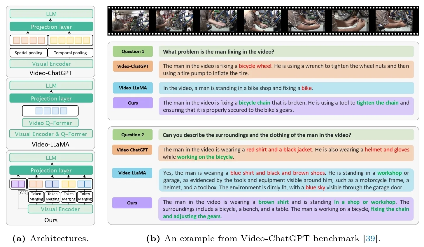
Method Setup and notation. Uniformly sample \(T\) frames, divide them into \(S\) short-term segments, each with \(K\) frames (\(T{=}S\!\cdot \!K\)). A frozen visual encoder (CLIP ViT-L/14 in the paper) extracts patch tokens for each frame. Let a frame-\(t\) token matrix be \[ P^{t}\in \mathbb {R}^{u\times d}\!, \] with \(u\) patch tokens and channel width \(d\).4 For a segment \(s\), collect its \(K\) frames’ tokens \begin {equation} \mathcal {V}^{s} \;=\; \big \{\,P^{t}\,\big \}_{t=1}^{K}\in \mathbb {R}^{K\times u\times d}. \label {eq:longvlm_vs} \end {equation}
Hierarchical token merging within each short segment. To build a compact, local representation while retaining details, LongVLM applies a hierarchical merging module \(\mathcal {G}(\cdot )\) inside each segment:
- Per-step partition. At merging step \(i\) (on a current token set of size \(R_i\)), randomly partition tokens into two disjoint sets \(\mathcal {P}_i\) and \(\mathcal {Q}_i\) with \(|\mathcal {P}_i|{=}r_i\), \(|\mathcal {Q}_i|{=}R_i{-}r_i\).
- Similarity. Split channels into \(C\) heads of width \(d_h\) (\(d{=}C\,d_h\)). For a token \(p^{(p_u)}\!\in \!\mathcal {P}_i\) and \(p^{(q_u)}\!\in \!\mathcal {Q}_i\), define the similarity by the head-averaged cosine: \begin {equation} a^{\,p^{u}q^{u}} \;=\; \frac {1}{C}\sum _{c=1}^{C} \cos \!\Big (p^{(p_u)}_{c},\,p^{(q_u)}_{c}\Big ), \label {eq:longvlm_cos} \end {equation} where \(p_c\) denotes the \(c\)-th head slice.
- Greedy pairing and merge. Choose the top-\(r_i\) pairs with the largest \(a^{\,p^{u}q^{u}}\) and average-pool each pair to a single token: \begin {equation} \tilde {t}^{(u)} \;=\; \mathrm {AvgPool}\!\Big (\,p^{(p_u)},\,p^{(q_u)}\!\Big ), \qquad u=1,\dots ,r_i. \label {eq:longvlm_merge} \end {equation} Concatenate these \(\{\tilde {t}^{(u)}\}_{u=1}^{r_i}\) with the unpaired tokens to obtain \(R_{i+1}{=}\,R_i{-}r_i\) tokens.
- Iterate. Repeat until a target budget \(M\) (tokens per segment) is reached. For segment \(s\) this yields a compact local feature \begin {equation} Z^{s} \;=\; \mathcal {G}(\mathcal {V}^{s}) \in \mathbb {R}^{M\times d}. \label {eq:longvlm_seg_z} \end {equation}
Stack segment features in temporal order to form the local sequence \begin {equation} \mathcal {L} \;=\; \big \{\,Z^{s}\,\big \}_{s=1}^{S} \in \mathbb {R}^{(MS)\times d}, \label {eq:longvlm_local_seq} \end {equation} which explicitly preserves the chronology of short-term segments across a long video.
Global semantic tokens from [CLS]. In parallel, LongVLM distills a global summary by collecting the [CLS] tokens of each frame from \(E\) (usually \(E=5\)) selected encoder layers \(\{x^{t}_{e}\}_{t=1}^{T}\) and averaging them over time per layer: \begin {equation} X_{e} \;=\; \mathrm {AvgPool}\!\Big (\{x^{t}_{e}\}_{t=1}^{T}\Big )\in \mathbb {R}^{d}, \quad e=1,\dots ,E,\qquad \mathcal {G}_{\mathrm {glob}} = \big \{X_{e}\big \}_{e=1}^{E}\in \mathbb {R}^{E\times d}. \label {eq:longvlm_global} \end {equation} These \(E\) tokens provide high-level, video-wide context (the gist) that complements the time-ordered, segment-level details in (24.41).
Concatenation, projection, and prompting the LLM. Concatenate global then local tokens (empirically superior to the reverse order): \[ [\;\mathcal {G}_{\mathrm {glob}} \,;\, \mathcal {L}\;] \in \mathbb {R}^{(E{+}MS)\times d}, \] and project them into the LLM input space with a learned linear layer only (visual encoder and LLM are frozen). The projected visual tokens are packed with the system prompt and user query and fed to the LLM to generate responses. This yields a long, information-rich visual stream for the LLM, avoiding the bottlenecks of heavy pre-LLM compression and preserving segment-level chronology.
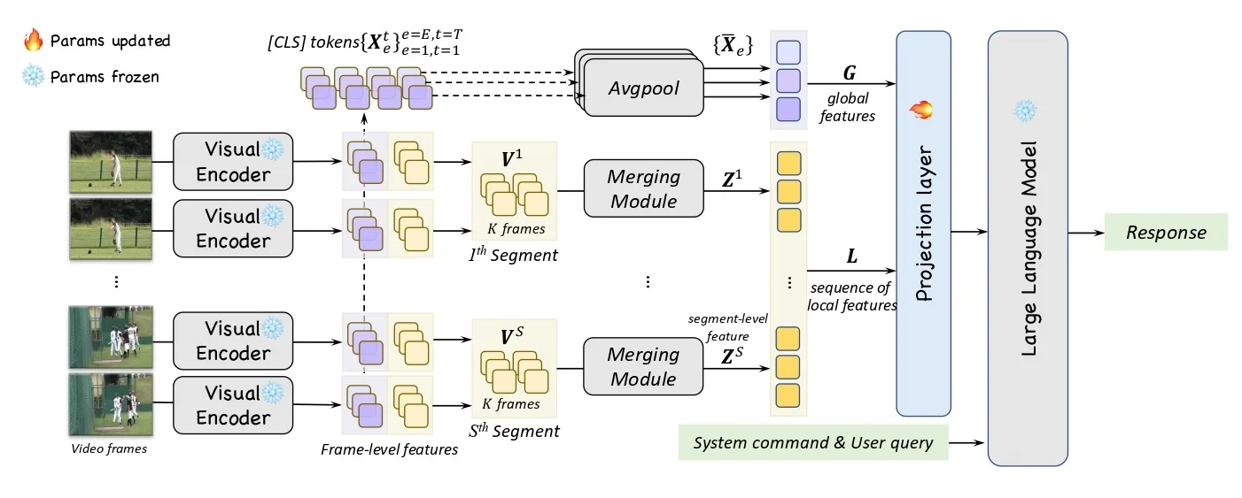
Algorithmic sketch (token merging within a segment)
# Pseudocode (faithful to the paper’s Sec. 3.2 definitions; not source code).
# Inputs: segment s with K frames, frame tokens {P^t in R^{u x d}}_{t=1..K}
# Output: Z^s in R^{M x d} (M << K*u)

def hierarchical_token_merging(P_list, M, C):
    # Flatten K x u tokens in the segment to a list T (length R0 = K*u)
    T = concat([P for P in P_list])          # T: [R0, d]
    R = len(T)
    while R > M:
        # Random disjoint partition (|P_i| = r_i, |Q_i| = R - r_i)
        P_i, Q_i = random_partition(T)
        # Head-averaged cosine similarity between every p in P_i and q in Q_i
        S = {}
        for p in P_i:
            for q in Q_i:
                S[(p, q)] = (1/C) * sum(cos(p[c], q[c]) for c in range(C))
        # Select top-|P_i| pairs by similarity (greedy, disjoint matching)
        matches = top_pairs(S, k=len(P_i))
        # Merge each matched pair by average pooling
        merged = [avg(p, q) for (p, q) in matches]
        # Unpaired tokens are carried over; update T and R
        unpaired = list(set(P_i + Q_i) - set([x for pair in matches for x in pair]))
        T = merged + unpaired
        R = len(T)
        # Return first M tokens in temporal order within the segment (implementation detail)
    return select_order_preserving(T, M)     # Z^s: [M, d]
Architecture & Implementation Details
- Backbone and LLM. LongVLM uses a frozen CLIP ViT-L/14 visual encoder and a frozen Vicuna-7B-v1.1 LLM, both initialized from LLaVA-7B-v1.1; only a single linear projection from vision features to the LLM input space is trained [713, Sec. 4.1]. The CLIP encoder operates at \(224{\times }224\) input resolution; with a \(14{\times }14\) patch size this yields \(u{=}256\) patch tokens per frame (plus [CLS]), and the similarity computation in the merging module uses \(C{=}16\) heads as stated in the paper [713, Sec. 3.2].
- Training setup. Finetuning is performed on the Video-ChatGPT-100K instruction dataset for \(3\) epochs with learning rate \(2{\times }10^{-5}\) and batch size \(32\); both the visual encoder and the LLM remain frozen while the projection layer is updated. The reported wall-clock for the full \(3\) epochs is approximately \(3\) hours on \(4\times \)A100-80GB GPUs [713, Sec. 4.1].
- Frame sampling and segmentation. During both training and inference, \(T{=}100\) frames are uniformly sampled per video at \(224^2\) resolution and divided into \(S{=}10\) short-term segments with \(K{=}10\) frames each (\(T{=}S\!\cdot \!K\)) [713, Sec. 4.1]. Within each segment, hierarchical token merging produces \(M\) compact local tokens (paper default \(M{=}30\)), while [CLS] tokens averaged over time from \(E\) selected CLIP layers provide global semantics (paper default \(E{=}5\) from the last five layers) [713, Sec. 3, Sec. 4.1].
- Token budget and ordering. The total number of visual tokens fed to the LLM per video is \((M\!\times \!S){+}E \,=\, 30\times 10 + 5 \,=\, 305\). Following the ablation, global tokens are concatenated before local tokens, i.e., [G,L], and the local sequence preserves the chronological order of segments (\(s{=}1\!\to \!S\)) when packed for the LLM [713, Fig. 2, Tab. 3]. The paper reports that [G,L] outperforms [L,G] on the Video-ChatGPT benchmark (Mean \(2.89\) vs. \(2.82\)).
- Projection and prompting. Visual tokens are linearly projected (projection is the only trainable module) and concatenated with system instructions and user queries to form the LLM input. This preserves a long, information-rich visual stream into the LLM without aggressive pre-LLM compression, aligning with the architectural rationale illustrated in Fig. 24.122.
Experiments and Ablations
Benchmarks and metrics LongVLM is evaluated on the Video-ChatGPT benchmark (500 ActivityNet-v1.3 videos, with 2,000 questions for each of five aspects: Correctness Information (CI), Detail Orientation (DO), Contextual Understanding (CU), Temporal Understanding (TU), Consistency (C)) and on zero-shot QA for ANET-QA, MSRVTT-QA, and MSVD-QA, reporting accuracy and generation quality scores.
| Method | Data | CI | DO | CU | TU | C | Mean |
|---|---|---|---|---|---|---|---|
| VideoChat [148] | 10M | 2.25 | 2.50 | 2.54 | 1.98 | 1.84 | 2.22 |
| LLaMA Adapter v2 [158] | 700K | 2.03 | 2.32 | 2.30 | 1.98 | 2.15 | 2.16 |
| Video LLaMA [142] | 10M | 1.96 | 2.18 | 2.16 | 1.82 | 1.79 | 1.98 |
| Video-ChatGPT [149] | 100K | 2.50 | 2.57 | 2.69 | 2.16 | 2.20 | 2.42 |
| Valley [159] | 234K | 2.43 | 2.13 | 2.86 | 2.04 | 2.45 | 2.38 |
| BT-Adapter [160] | 10M | 2.16 | 2.46 | 2.89 | 2.13 | 2.20 | 2.37 |
| BT-Adapter [160] | 10M+100K | 2.68 | 2.69 | 3.27 | 2.34 | 2.46 | 2.69 |
| LongVLM [117] | 100K | 2.76 | 2.86 | 3.34 | 2.39 | 3.11 | 2.89 |
| Method | Data | ANET-QA Acc. | ANET-QA Score | MSRVTT-QA Acc. | MSRVTT-QA Score | MSVD-QA Acc. | MSVD-QA Score |
|---|---|---|---|---|---|---|---|
| FrozenBiLM [161] | 10M | 24.7 | — | 16.8 | — | 32.2 | — |
| VideoChat [148] | 10M | 26.5 | 2.2 | 45.0 | 2.5 | 56.3 | 2.8 |
| LLaMA Adapter v2 [158] | 700K | 34.2 | 2.7 | 43.8 | 2.7 | 54.9 | 3.1 |
| Video LLaMA [142] | 10M | 12.4 | 1.1 | 29.6 | 1.8 | 51.6 | 2.5 |
| Video-ChatGPT [149] | 100K | 35.2 | 2.7 | 49.3 | 2.8 | 64.9 | 3.3 |
| Valley [159] | 234K | 45.1 | 3.2 | 51.1 | 2.9 | 60.5 | 3.3 |
| BT-Adapter [160] | 10M+100K | 45.7 | 3.2 | 57.0 | 3.2 | 67.5 | 3.7 |
| LongVLM [117] | 100K | 47.6 | 3.3 | 59.8 | 3.3 | 70.0 | 3.8 |
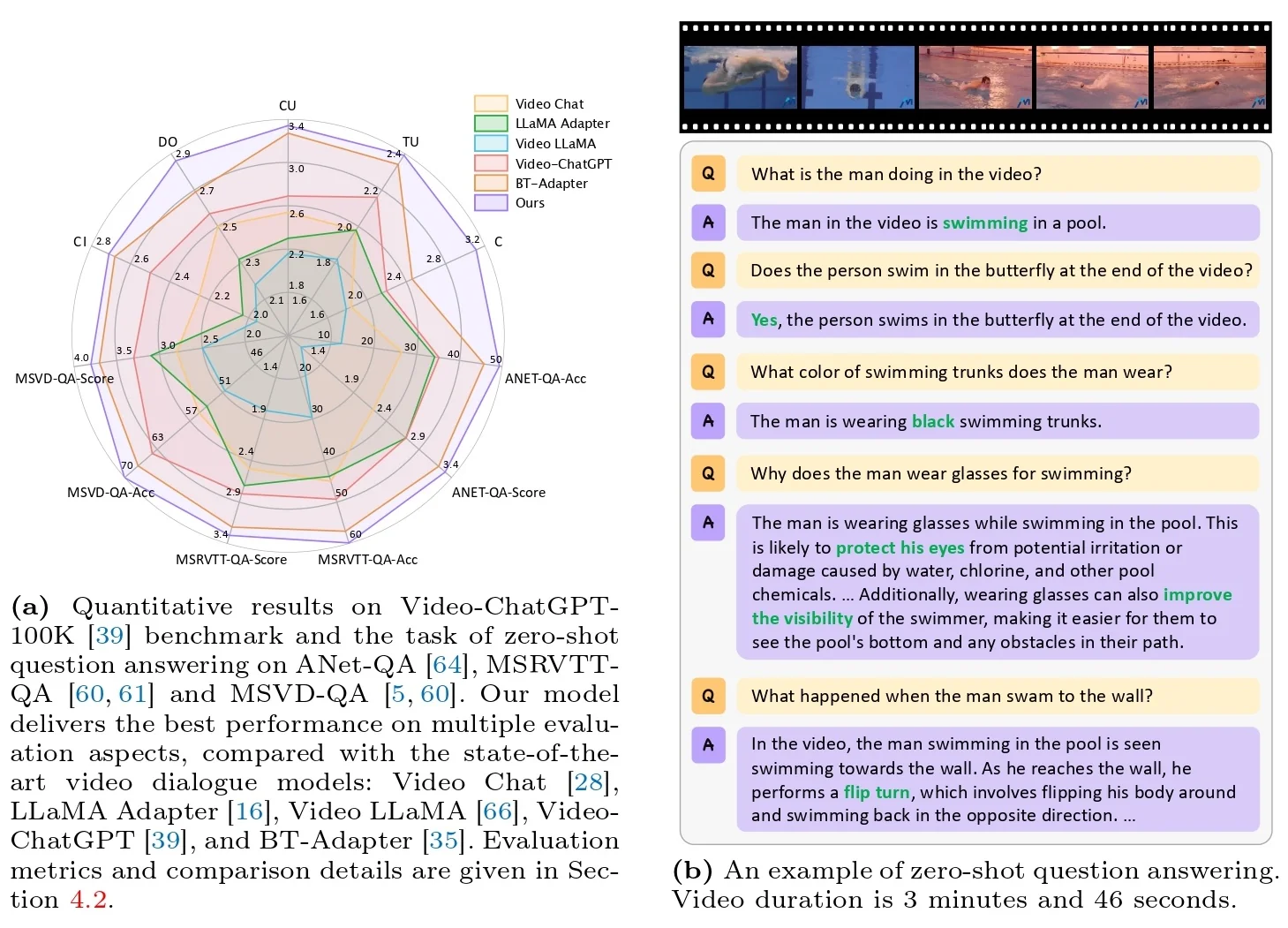
Ablations LongVLM conducts controlled ablations on: (i) local feature construction and global fusion, (ii) the per-segment token budget \(M\), and (iii) the number of selected encoder layers \(E\) used to form global [CLS] tokens [713, Sec. 4.3]. The key findings are summarized below.
| Variants | Local | Global | CI | DO | CU | TU | C | Mean |
|---|---|---|---|---|---|---|---|---|
| Pooling | Yes | No | 2.53 | 2.64 | 3.13 | 2.29 | 2.61 | 2.64 |
| Merging | Yes | No | 2.62 | 2.74 | 3.15 | 2.23 | 2.86 | 2.72 |
| [L, G] | Yes | Yes | 2.69 | 2.81 | 3.31 | 2.31 | 2.99 | 2.82 |
| [G, L] | Yes | Yes | 2.76 | 2.86 | 3.34 | 2.39 | 3.11 | 2.89 |
Local & global synergy. Replacing naive 3D pooling with hierarchical token merging improves Mean from \(2.64\) to \(2.72\). Combining local and global tokens further boosts performance, and ordering matters: prepending global tokens [G, L] achieves the best Mean of \(2.89\), matching the main result in Table 24.65.
Per-segment token budget \(M\). Increasing \(M\) improves the Video-ChatGPT Mean up to \(\approx 30\) tokens/segment (Mean \(2.89\) at \(M{=}30\)), while GPU memory remains nearly flat (e.g., \(\approx 14.86\) GB at \(M{=}30\) on ANET-QA), with no further gains at \(M{=}40\) [713, Tab. 4].
Global layers \(E\). Using global [CLS] tokens aggregated from the last \(E{=}5\) visual encoder layers yields the strongest balance (Mean \(2.89\)); smaller (\(E{=}1\)) or larger (\(E{\geq }10\)) selections slightly underperform [713, Tab. 5].
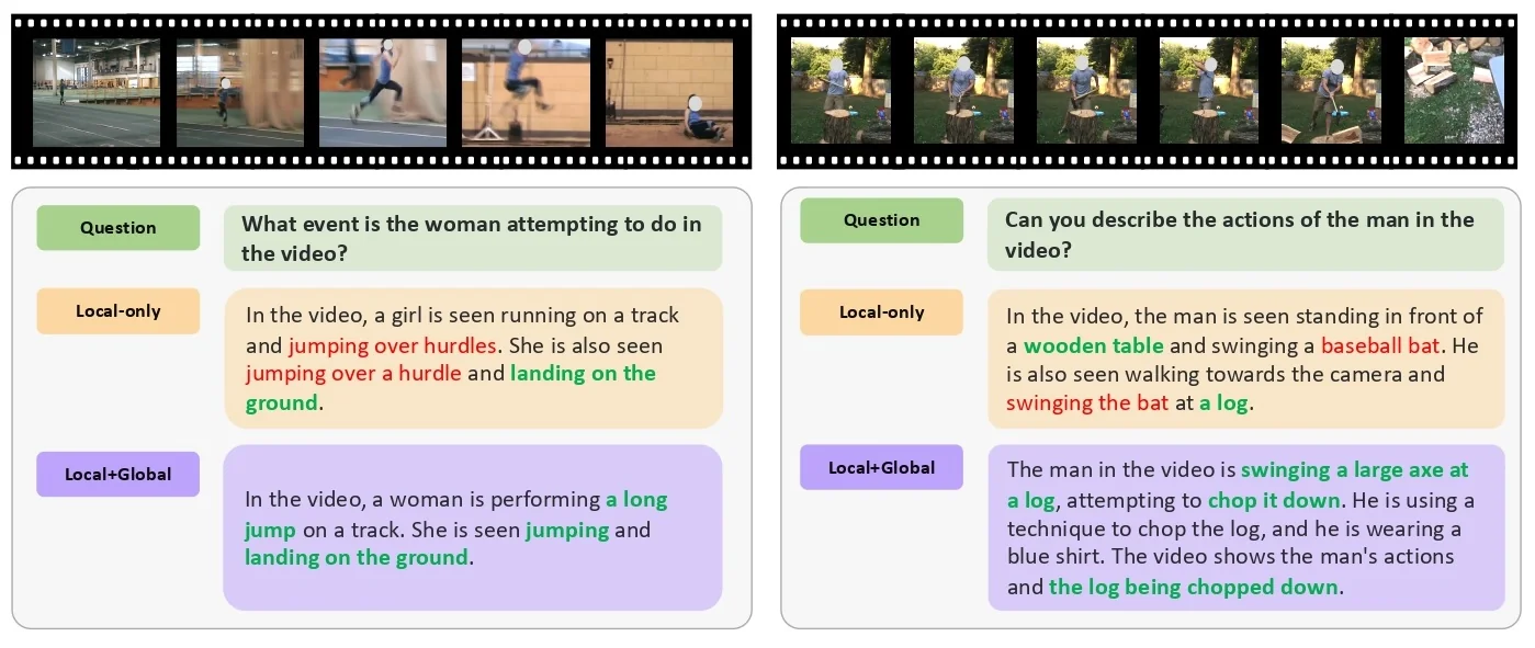
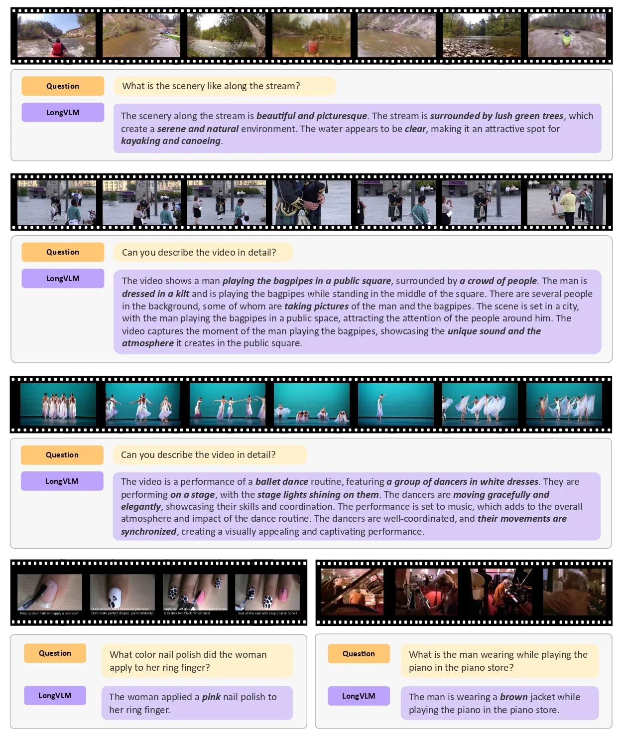
- Fixed per-segment budget. The token budget \(M\) per segment is static; highly dynamic or sparse videos may benefit from adaptive merging (retrieval- or saliency-guided) that varies the number of local tokens across segments.
-
Cosine-based merging. Merging uses head-averaged cosine similarity and average pooling, which is simple and efficient but can still lose fine-grained rare cues. More expressive, learnable merging or content-aware reweighting could further preserve details.
- Global token selection. Global semantics rely on [CLS] tokens from fixed encoder layers; while effective, other summary signals (e.g., learned cross-frame prototypes or absolute timestamps) may improve localization in long, irregular streams.
- Frozen backbone and LLM. The frozen CLIP and LLM promote stability and training efficiency, but may limit domain adaptation. Lightweight adapters or partial tuning could help in specialized domains without sacrificing efficiency.
- Scaling to extreme durations. Although LongVLM already feeds a longer visual sequence than prior Video-LLMs, very long videos still stress the LLM context window. Subsequent methods (e.g., the next subsection on LWM) explore sparse/blockwise attention and retrieval to scale beyond hundreds of tokens.
Bridge to LWM. LongVLM demonstrates that preserving a longer, ordered stream of local tokens plus a few global tokens substantially reduces hallucinations and improves temporal grounding without retraining the LLM or the visual encoder. The next method, LWM, pushes sequence length even further via scalable attention patterns and memory mechanisms designed for million-token contexts.
Enrichment 24.10.3: LWM: Blockwise RingAttention for Million-Token Contexts
Motivation Long-context Video-LLMs and MLLMs have historically been constrained by quadratic-cost attention and modality-specific projections, which force aggressive pre-LLM compression and limit temporal grounding over hours of content. LWM [375] is proposed as a unified, autoregressive world model that scales the context window to \(1\)M tokens while operating directly on discrete vision tokens and text within a single Transformer, enabling long-video understanding and retrieval at million-length scale.
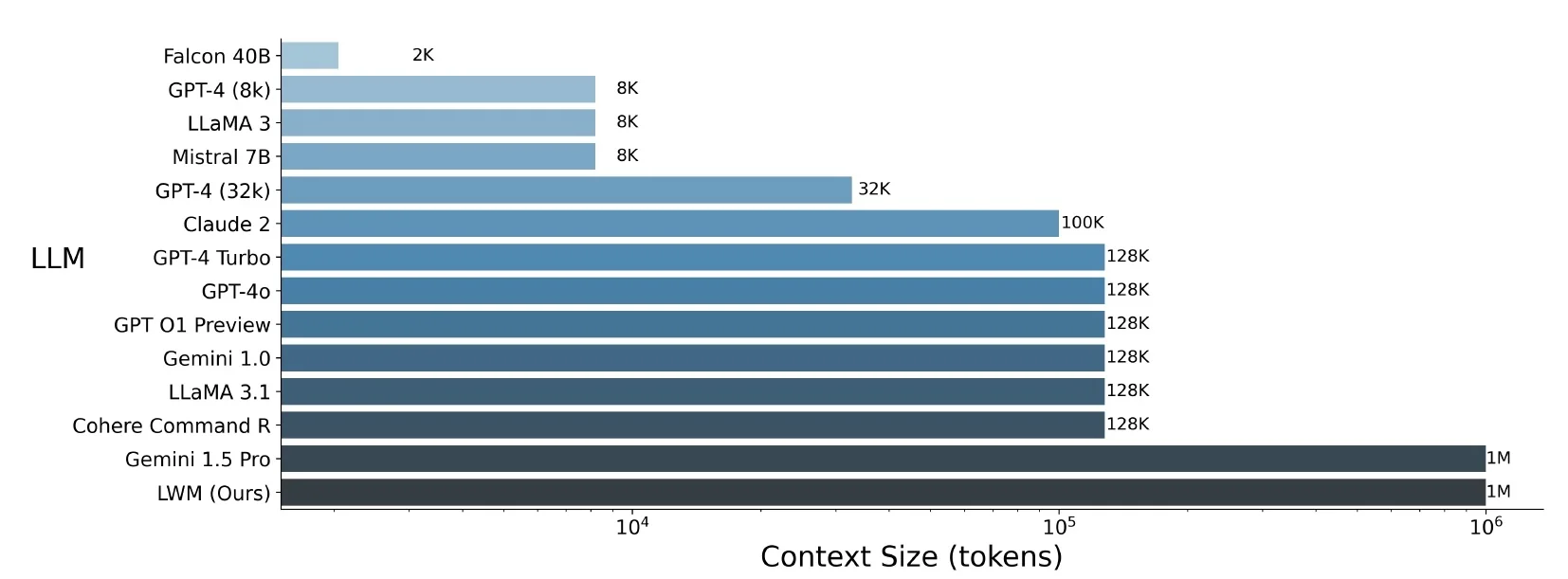
Method Unified token space with discrete vision tokens. LWM maps language and vision into a single, discrete token space processed by one causal Transformer [375]. Text is tokenized with a standard BPE tokenizer; each image frame is tokenized by a pretrained VQGAN into a \(16{\times }16\) grid of codebook indices (i.e., \(256\) tokens for a \(256{\times }256\) frame). Vision spans are bracketed by special tokens <vision> and </vision>, with per-frame and end-of-vision delimiters <eof> and <eov> to mark boundaries. After concatenation, the model autoregressively predicts the next token over the joint vocabulary (text subwords \(+\) vision codes), enabling any-to-any understanding and generation across text, image, and video without a separate vision\(\to \)LLM projection layer.5 Intuition: VQGAN turns pixels into a compact visual alphabet. Once both modalities are “just tokens”, a single decoder can read and write text, images, and videos in one sequence, with modality switches indicated by delimiters [375, Sec. 2, Fig. 3].
Training Curriculum The context window is not expanded to one million tokens in a single step. Training advances through a small ladder of maximum sequence caps (for example, \(32\mathrm {K}\rightarrow 64\mathrm {K}\rightarrow 128\mathrm {K}\rightarrow 256\mathrm {K}\rightarrow 512\mathrm {K}\rightarrow 1\mathrm {M}\)). At each rung, the very same Transformer is optimized as usual; what changes is (i) how inputs are converted to tokens and then packed up to the current cap, and (ii) how positional encodings are scaled so they remain well behaved at the longer horizon [375, Sec. 3.1]. The model is fine-tuned at one cap until stable, then training resumes from that checkpoint at the next cap, rather than starting from scratch.
From images/videos to tokens (step by step).
- 1.
- Start with raw data (and how to handle long videos). An image arrives
as \(I \in \mathbb {R}^{C\times H\times W}\) (e.g., \(3\times 256\times 256\)); a video as \(V \in \mathbb {R}^{T\times C\times H\times W}\) (e.g., \(T{=}120\) frames at \(4\) FPS for a \(30\)s clip). Before
tokenization, apply the minimal preprocessing required by the frozen
VQGAN tokenizer: resize/center-crop frames to \(256{\times }256\) and normalize pixel
values as expected by the tokenizer (e.g., to \([0,1]\) or \([-1,1]\), per its training). The
goal in this step is not feature engineering but simply to ensure frames
are in the canonical format the tokenizer expects so that code indices
are meaningful.
How to fit long videos under the current context cap \(N_{\max }\). In sub-stage training with cap \(N_{\max }\) (e.g., \(32\mathrm {K}\), \(64\mathrm {K}\), \(\ldots \), \(1\mathrm {M}\) tokens), each packed training sequence must satisfy a length budget. Let \(L_{\mbox{text}}\) be the text tokens in the packed sequence (prompt, question, target, etc.) and \(L_{\mbox{misc}}\) be delimiters and any extra small fields. The remaining vision budget is \[ B_{\mbox{vis}} \;=\; N_{\max } - L_{\mbox{text}} - L_{\mbox{misc}}. \] Each frame contributes approximately \(c_{\mbox{frame}}\approx 256 + c_{\mbox{delim}}\) tokens, where \(256\) comes from the \(16{\times }16\) VQGAN codes and \(c_{\mbox{delim}}\) accounts for <eof> and occasional boundary tokens (typically a small constant). This gives a maximum number of frames that can fit under the current cap: \[ T_{\max } \;=\; \big \lfloor B_{\mbox{vis}} / c_{\mbox{frame}} \big \rfloor . \] If the raw video has \(S\) seconds and original FPS \(f_{\mbox{raw}}\) (so \(T_{\mbox{raw}} \!=\! S f_{\mbox{raw}}\) frames), reduce temporal density as follows:
- (a)
- Temporal subsampling (preferred first). Choose a target FPS \[ f_{\mbox{target}} \;=\; \min \!\Big (f_{\mbox{raw}},\, \big \lfloor T_{\max }/S \big \rfloor \Big ), \] and uniformly sample frames at stride \(\lfloor f_{\mbox{raw}}/f_{\mbox{target}}\rfloor \). This preserves chronological order while shrinking the token count linearly with FPS.
- (b)
- Contiguous windowing (if still too long). If even \(f_{\mbox{target}}{=}1\) FPS would exceed the budget, extract a contiguous window of \(T_{\max }\) frames (e.g., pick a random start time each epoch) and discard the rest for this batch. On subsequent steps, sample a different window so that, across training, the model still sees the entire clip.
- (c)
- Sliding-window splitting (optional). Alternatively, split the video into overlapping windows of length \(\le T_{\max }\) (e.g., \(50\%\) overlap) and treat each window as a separate training example across iterations. This increases coverage without violating the cap.
Why reduce FPS or window? Each additional frame adds \(\approx 256\) tokens. Without subsampling/windowing, long clips would blow past \(N_{\max }\) early in the curriculum (e.g., \(32\mathrm {K}\)), making batches impossible to pack and destabilizing optimization. Reducing FPS trades temporal density for sequence feasibility while preserving order; windowing then ensures that, over epochs, the model eventually observes all parts of the video.
Concrete example. Suppose \(N_{\max }{=}64{,}000\), \(L_{\mbox{text}}{=}1{,}500\), \(L_{\mbox{misc}}{=}500\), so \(B_{\mbox{vis}}{=}62{,}000\). With \(c_{\mbox{frame}}\!\approx \!257\), we get \(T_{\max }{=}\lfloor 62{,}000/257 \rfloor {=}241\) frames. For a \(120\)s clip at \(f_{\mbox{raw}}{=}4\) FPS (\(T_{\mbox{raw}}{=}480\)), set \(f_{\mbox{target}}{=}\lfloor 241/120 \rfloor {=}2\) FPS and sample \(\approx 240\) frames uniformly. If the clip were \(1{,}200\)s long, even \(f_{\mbox{target}}{=}1\) FPS would exceed the budget; in that case, take a contiguous window of \(T_{\max }{=}241\) frames (about four minutes) this step, and a different window next time.
- 2.
- Tokenize vision. A frozen VQGAN encodes each \(256{\times }256\) frame into a \(16{\times }16\) grid of codebook indices (i.e., \(256\) discrete tokens per frame). For videos, concatenate frames in order and insert <eof> between successive frames; wrap the whole span with <vision> and </vision>, and close with <eov>. Example (image): <vision> [256 codes] </vision><eov>. Example (video with \(T\) frames): <vision> \([256]\,\texttt{<eof>}\,\cdots \,\texttt{<eof>}\,[256]\) </vision><eov>. The resulting visual length is roughly \(256T + O(T)\) tokens (the \(O(T)\) comes from delimiters).
- 3.
- Tokenize text. Apply BPE to captions, instructions, transcripts, or questions to obtain standard text tokens. These share the same embedding/output layers as the vision codes once the vocabulary is extended.
- 4.
- Interleave modalities. Build a single sequence that mixes text and vision in
the causal order required by the task, using delimiters as punctuation so
the decoder can switch modalities.
- Captioning. [Prompt tokens] <vision> [image codes]
</vision><eov>
[Target caption tokens]. - Video QA. [Question tokens] <vision> [frame\(_1\) codes] <eof> \(\cdots \) [frame\(_T\) codes] </vision><eov> [Answer tokens].
- Conditional generation. [Instruction tokens] \(\rightarrow \) the model emits image/video codes that a VQGAN decoder later turns into pixels.
- Captioning. [Prompt tokens] <vision> [image codes]
</vision><eov>
- 5.
- Pack to the current cap. Let \(N_{\max }\) be the current sub-stage cap (e.g., \(32\mathrm {K}\), \(64\mathrm {K}\), \(\ldots \), \(1\mathrm {M}\)).
Construct training sequences by concatenating one or more interleaved
examples until the total length reaches (or slightly under-fills) \(N_{\max }\), and apply a
causal mask.
- If a single example fits (\(\leq N_{\max }\)). Pack it as is; if there is remaining space, append another short example or leave the remainder masked to the end of the packed sequence.
- If a single example exceeds \(\boldsymbol {N_{\max }}\). Use one of the above windowing strategies so long examples still contribute signal at the current cap.
- Mixture of lengths. Because real examples vary, each batch naturally contains short and near-cap sequences. This length mixture helps the model retain short-context competence while learning to exploit very long histories.
- Concrete packing example. Suppose \(N_{\max }=64{,}000\). A video-QA example tokenizes to \(40{,}000\) tokens; an image-captioning example tokenizes to \(8{,}000\); a text-only excerpt tokenizes to \(14{,}000\). Concatenate in order: \(40{,}000 + 8{,}000 + 14{,}000 = 62{,}000 \leq 64{,}000\). The remaining \(2{,}000\) tokens are left masked or filled with a very short snippet if available.
Intuition. Think of each packed training sequence as a fixed-size “page.” Long stories are read in excerpts (windows), short notes are combined on the same page, and across many pages the model still sees the whole book.
- 6.
- Optimize and repeat. Feed the packed sequence \(X\in \mathbb {R}^{\leq N_{\max }\times d}\) into the causal Transformer and train with next-token cross-entropy over the joint vocabulary (text BPE IDs + vision code IDs). The VQGAN is always frozen; the Transformer and the shared embedding/output layers are updated so the model learns to both consume and emit vision codes alongside text. When validation stabilizes at the current cap, increase the cap to the next rung, rescale RoPE so positional geometry remains smooth at the longer horizon, resume from the latest checkpoint, and continue. Over epochs, windowed sampling ensures that even examples longer than \(N_{\max }\) are eventually seen in full, just not all at once.
Why the length ladder helps. Jumping straight to \(1\)M tokens forces the network to master long-range structure it has never seen while also maintaining local competence; optimization often becomes unstable. By first training at \(32\mathrm {K}\), the model learns reliable local and mid-range patterns (sentences, short dialogues, tens of frames). Moving to \(64\mathrm {K}\) and \(128\mathrm {K}\) extends these habits to chapters and minutes of video. Each step “warms up” the next, so the final \(1\mathrm {M}\) stage mostly requires adapting to span-wide dependencies rather than discovering everything at once.
What it means to scale RoPE. RoPE encodes position \(m\) by rotating each 2-D channel pair of a head vector with angle \[ \phi _i(m)=m\,\omega _i,\qquad \omega _i=\Theta _{\mbox{base}}^{-\,2i/d_h},\quad i=0,\ldots ,\tfrac {d_h}{2}-1, \] using \[ R(\phi )= \begin {bmatrix} \cos \phi & -\sin \phi \\ \sin \phi & \cos \phi \end {bmatrix}. \] With \(q_m^{(i)},k_n^{(i)}\in \mathbb {R}^2\), RoPE has the relative property \[ \big \langle R(\phi _i(m))\,q_m^{(i)},\,R(\phi _i(n))\,k_n^{(i)}\big \rangle \;=\; \big \langle q_m^{(i)},\,R\big ((n-m)\,\omega _i\big )\,k_n^{(i)}\big \rangle , \] so attention depends on the offset \(\Delta =n-m\) via rotations by \(\Delta \,\omega _i\).
Why naïve extrapolation breaks. If the context grows (e.g., \(32\mathrm {K}\!\to \!1\mathrm {M}\)) but \(\Theta _{\mbox{base}}\) stays fixed, high–frequency channels wrap many times around the unit circle. Very distant tokens can become spuriously similar (phase aliasing), hurting long-range reasoning.
LWM’s scaling rule (paper-faithful). Let \(s=\tfrac {N_{\mbox{new}}}{N_{\mbox{old}}}\). LWM rescales RoPE proportionally to the new context by enlarging the base: \[ \Theta _{\mbox{base}}^{\mbox{new}}=\Theta _{\mbox{base}}^{\mbox{old}}\cdot s \quad \Longleftrightarrow \quad \omega _i^{\mbox{new}}=\omega _i/s. \] Equivalently (index view), keep \(\Theta _{\mbox{base}}\) and slow the index: \[ \phi _i^{\mbox{new}}(m)=\tfrac {m}{s}\,\omega _i. \] In either view, \[ \big \langle R(\phi _i^{\mbox{new}}(m))q^{(i)},\,R(\phi _i^{\mbox{new}}(n))k^{(i)}\big \rangle = \big \langle q^{(i)},\,R\!\big (\tfrac {(n{-}m)\,\omega _i}{s}\big )k^{(i)}\big \rangle , \] so the effective distance becomes \(\Delta _{\mbox{eff}}=\Delta /s\). Example: from \(32\mathrm {K}\) to \(1\mathrm {M}\), \(s{\approx }32\); a gap of \(\Delta {=}100\mathrm {K}\) “feels like” \(\Delta _{\mbox{eff}}\!\approx \!3.1\mathrm {K}\) at the shorter cap—preventing wrap-around while preserving local geometry.
Practical note (common variant). Some implementations use a single slowdown exponent \(\alpha \!\in \![0,1]\) (often \(0.5\)) so that \(\Theta _{\mbox{base}}^{\mbox{new}}=\Theta _{\mbox{base}}^{\mbox{old}}\cdot s^{\alpha }\) (equivalently \(\Delta _{\mbox{eff}}=\Delta /s^{\alpha }\)). Use \(\alpha {=}1\) to match the paper’s “proportional to context” description; smaller \(\alpha \) can be used as an engineering tweak without changing the derivation above.
Blockwise RingAttention for exact million-length attention. Let \(X\!\in \!\mathbb {R}^{N\times d}\) be the input sequence (with \(N\) up to \(10^6\)) and \(h\) heads of size \(d_h{=}d/h\). Standard causal self-attention \[ \mathrm {Attn}(Q,K,V)\;=\;\mathrm {Softmax}\!\Big (\tfrac {QK^\top }{\sqrt {d_h}}+\mathrm {mask}\Big )\,V \] is exact but materializing \(QK^\top \) and a full KV cache is prohibitive at \(N{=}10^6\). Blockwise RingAttention [375, Sec. 3.1] partitions the sequence into \(G\) contiguous blocks of size \(B\) so \(N{=}GB\). Devices are arranged in a logical ring. Each device holds one query block \(g\) and iteratively streams key/value blocks \((K^{(g')},V^{(g')})\) from all other blocks around the ring:
- 1.
- Compute attention for local pairs \((Q^{(g)},K^{(g)},V^{(g)})\) with a fused kernel (e.g., FlashAttention), applying the causal mask to exclude future positions within the block.
- 2.
- Receive the next \((K^{(g')},V^{(g')})\) from the neighbor, compute the masked cross-block contribution \(\mathrm {Softmax}\!\big (Q^{(g)}{K^{(g')}}^{\!\top }/\sqrt {d_h}+\mathrm {mask}\big )V^{(g')}\), and accumulate it into the output for block \(g\).
- 3.
- Forward \((K^{(g')},V^{(g')})\) to the next device; repeat until all \(G\) key/value blocks have been visited exactly once.
Because each \((\mbox{query block},\mbox{key block})\) pair is covered once under the causal mask, the result is mathematically identical to dense attention. Only \(O(B)\) KV tokens live on a device at any moment; communication of streamed KV is overlapped with per-block compute, yielding high throughput on large device meshes [375, Sec. 3.1]. Intuition: Think of a block relay: each device keeps its queries and “meets” every other block’s keys/values as they circulate around the ring, accumulating the same full-context result without storing the entire sequence.
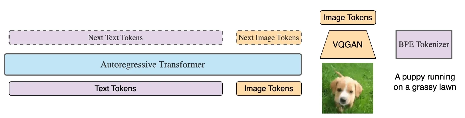
Discrete vision tokens, VQGAN, and projection-free learning. LWM makes vision “native” to the decoder by adding visual tokens—not projected features—to its vocabulary. A pretrained, frozen VQGAN maps each \(256{\times }256\) frame to a \(16{\times }16\) grid of codebook indices (flattened to \(256\) integers) [375, Fig. 3]; videos are tokenized frame-by-frame, concatenated with <eof> between frames, wrapped by <vision>...</vision>, and closed with <eov>. These indices are treated exactly like text BPE IDs: the Transformer’s shared embedding matrix (and tied LM head) is expanded to include the vision codebook plus boundary tokens, and then trained end-to-end so the same decoder models \[ p_\theta (x_{t+1}\mid x_{\le t}),\quad x_t \in \mathcal {V}_{\mbox{text}} \cup \mathcal {V}_{\mbox{vis}} \cup \{\texttt{<vision>},\texttt{</vision>},\texttt{<eof>},\texttt{<eov>}\}. \] No CLIP-style projector or adapter is required because VQGAN already produces discrete IDs; all tokens live in one space, and modality switches are cued by simple delimiters rather than separate heads. During Stage II, mixed text+vision sequences are fed under teacher forcing with a single cross-entropy over the joint vocabulary. The decoder thereby learns to interpret codes (e.g., answer questions conditioned on long spans of frames across <eof> boundaries) and to emit coherent code sequences for conditional generation; predicted codes can be rendered back to pixels by the frozen VQGAN decoder. Because the tokenizer never changes, the meaning of each code ID is stable throughout training, so learning concentrates where it matters—on the Transformer’s embeddings and attention—avoiding “interface drift” and collapse that can arise when a learned projector shifts. Intuition. VQGAN supplies a fixed “visual alphabet.” Once images and videos are written as tokens, the LLM simply learns a larger language: just as it acquires word/subword syntax, it acquires visual “subword” syntax (spatial regularities within a frame; temporal patterns across <eof>) in the same autoregressive stream.
Architecture & Implementation Details
Implementation summary.
- Backbone. A standard decoder-only Transformer (7B) serves as the core model for both text-only and multimodal training, optimized autoregressively over interleaved token streams [375].
- What is trained vs. frozen. The Transformer (initialized from a strong long-context text model) is trained across both curriculum stages; the VQGAN vision tokenizer remains frozen. The token embedding and output (softmax) layers are expanded to include the vision codebook and trained so the decoder can emit and consume visual tokens [375, Sec. 4].
- Vision tokenizer. A pretrained VQGAN [149] (from aMUSEd) discretizes images of size \(256{\times }256\) into a \(16{\times }16\) grid of code indices (256 tokens per frame). Videos are tokenized frame-by-frame and concatenated in temporal order.
- Special tokens. Vision spans are wrapped with <vision>...</vision>; per-frame boundaries use <eof>; the end of an image or the last frame of a video uses <eov>. These delimiters teach the single decoder to switch modalities inside very long sequences [375, Sec. 4].
-
Attention scaling. Million-length context is enabled by Blockwise RingAttention (exact dense attention via blockwise ring scheduling) fused with FlashAttention-style kernels for high MFU, while rotary position embeddings (RoPE) use a scaled base parameter matched to the target context length for stability up to \(1\)M tokens [375, Sec. 3.1].
- Training curriculum. Stage I grows a text-only model from \(32\)K to \(1\)M context on long-form documents, progressively rescaling the RoPE base and initializing each length from the previous one. Stage II introduces multimodality by interleaving text with image/video code sequences and continues progressive length increases (e.g., short sequences for stabilization, then to chat/long-form settings), preserving short-context accuracy while extending the window [375, Sec. 3.1, Sec. 4].
- Data construction. Stage I uses long-form book-style corpora to train long-range language modeling. Stage II mixes large-scale image–text sources (e.g., LAION-2B-en, COYO-700M; images filtered to \(\geq 256\) px) with video–text sources (e.g., WebVid10M, InternVid10M); frames are discretized by VQGAN and packed with text using the modality delimiters, and pairs are packed to target lengths with randomized text–vision order to cover captioning and generation directions [375, Sec. 4].
- Why it works. Discretizing vision removes modality-specific projectors and allows a single decoder to model text and vision uniformly in one token space, while RingAttention preserves exact full-context interactions at the million-token scale so long-range dependencies in hour-long videos and long documents remain accessible during training and inference [375, Sec. 2, Sec. 3.1].
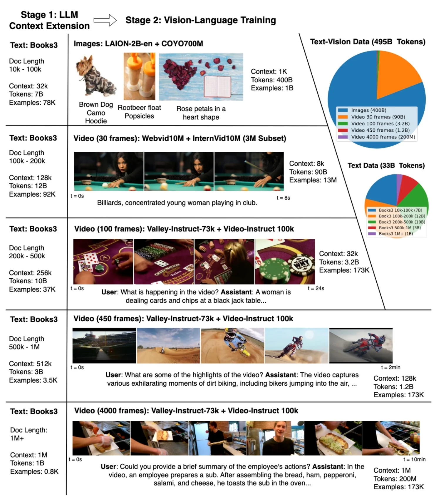
Experiments and Ablations
Long-context retrieval (needle and multi-needle) LWM maintains strong needle-in-a-haystack retrieval across the full 1M-token window: accuracy is high and largely insensitive to where the needle is placed in the sequence. In multi-needle variants (several facts inserted, one question requiring synthesis), LWM remains competitive as the number of required facts grows, reflecting that exact full-context attention (via RingAttention) reliably surfaces distant evidence rather than relying on truncation or heuristics. The paper’s plot uses a mixed x-axis (0–128K log, 128K–1M linear) to show that performance does not collapse as position approaches the 1M boundary.
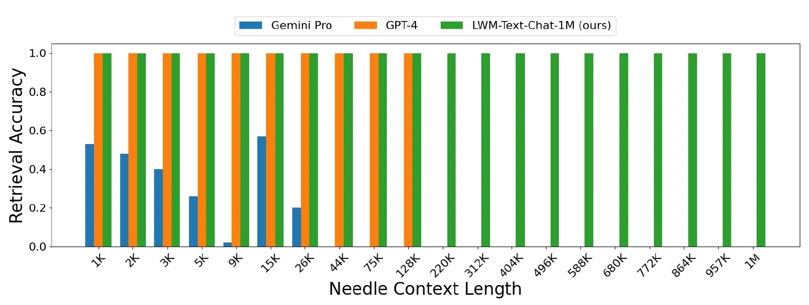
Language tasks at short context As the context is expanded from \(32\)K to \(1\)M, short-context language benchmarks (ARC, HellaSwag, MMLU, OpenBookQA) remain broadly stable (Table 1 in the paper), indicating that the length curriculum and mixed-length packing preserve near-field skills while extending the horizon.
LOFT benchmarks (512K) On long-document retrieval and RAG (LOFT), LWM at \(512\)K outperforms strong baselines on Quora and NQ and is substantially ahead on HotPotQA, highlighting the benefit of attending to the whole corpus chunk at once (no truncation artifacts). The reported scores are:
Long-video understanding On Long Video-MME, LWM-1M (7B) processes up to \(\leq 1800\) frames and achieves strong results, including \(60.8\) on the \(30\)–\(60\) min split (Table 4 in the paper). Intuitively, the model can downsample and still keep the entire narrative in-context, so answers can depend on events far apart in time without losing earlier evidence.
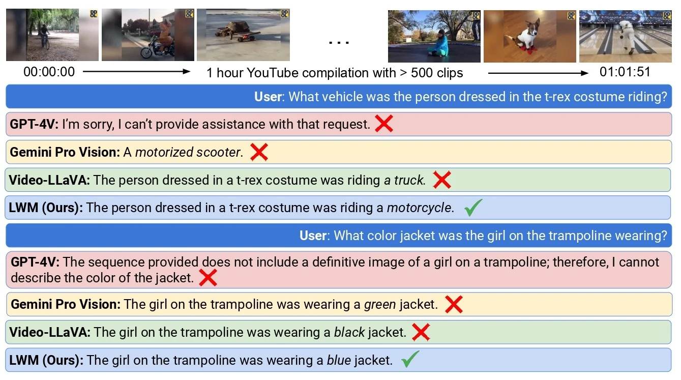
Generation Because vision is discretized, the same autoregressive decoder that models text can also emit image and short video code sequences conditioned on text. Decoding those codes through the (frozen) VQGAN yields images and simple clips with coherent local dynamics (e.g., fireworks, waves). This is a direct consequence of training a single next-token model over a joint vocabulary of text and vision IDs.
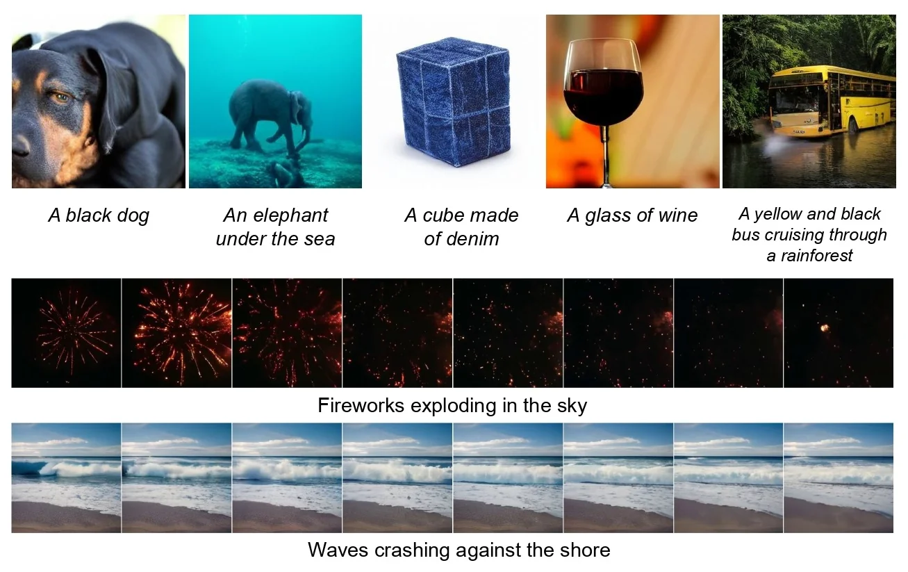
Limitations and Future Work
- Compute and hardware demands. Million-length training and inference rely on large device meshes and careful kernel fusion; although attention is exact, the system requirements are substantial and may limit accessibility.
- Vocabulary expansion and modality balance. Incorporating a vision codebook expands the vocabulary and requires curriculum tuning to preserve strong text performance while learning vision tokens at scale.
- Token efficiency for very long videos. Per-frame tokenization at fixed resolution (256 codes/frame) can become costly for multi-hour content; integrating adaptive frame rates, token pruning, or content-aware compression could further extend effective context.
- Position encoding extrapolation. Scaled RoPE is simple and empirically stable, but principled positional schemes tailored for interleaved multimodal streams may further improve generalization at extreme lengths.
Enrichment 24.11: Specialized Directions
Beyond short-clip classification, several specialized tasks push distinct modeling frontiers.
Temporal detection and localization. Here the goal is not only to recognize which action occurs but also to determine when it starts and ends in long, untrimmed videos. Methods include two–stage pipelines (proposal \(\rightarrow \) classification) as well as end-to-end transformer models that directly predict temporal boundaries.
Video diffusion models. Diffusion models extend from images to video by introducing temporal consistency modules that enforce smooth frame-to-frame evolution. A representative system, Video Diffusion Models (VDM), demonstrates high-fidelity synthesis and editing by scaling latent diffusion to temporal data [46].
Multimodal alignment. Video rarely comes alone; audio, depth, and infrared cues are often available. LanguageBind learns a unified embedding space that aligns video with multiple sensing modalities to language, broadening supervision and enabling stronger transfer across tasks [741].
Layered, object-centric video effects (Omnimatte family). Omnimatte pioneered layered mattes that jointly capture objects and their visual effects (e.g., shadows, reflections) from monocular video, enabling editing and compositing [408]. The follow-up OmnimatteRF extended this idea to neural radiance fields, allowing layered decomposition in a 3D-aware representation [409].
Related and emerging directions. Efficiency-oriented backbones (e.g., UniFormerV2 [355]) and distillation-style masked pretraining (e.g., Masked Video Distillation [691]) are widely adopted in practice. Long-form video QA (e.g., EgoSchema) and holistic reasoning benchmarks (e.g., VideoMind) continue to push models toward higher-level cognition. Finally, recent open and commercial diffusion-based systems such as VideoCrafter, Runway Gen-2, and Pika increasingly inform pipelines for video synthesis and editing.
1See also VideoChat [148] and Video-ChatGPT [149] for vision-only video dialogue.
2See Fig. 1 and Sec. 1 of [155] for the compute\(\leftrightarrow \)duration trade-off and motivation.
3“Uniform half”—augmenting roughly \(50\%\) of layers by alternating standard and memory attention—yields the best trade-off in Table 1(c) of [155].
4LongVLM follows the LLaVA family for vision\(\to \)language alignment, but keeps the encoder and LLM frozen and trains only a projection, avoiding costly end-to-end tuning.
5Using discrete VQGAN indices as tokens removes the need for a continuous vision\(\to \)language projector, but requires extending the embedding and output (softmax) layers to include the vision codebook and optimizing them jointly so the decoder learns the distribution over visual codes; see [157, Fig. 3].