Lecture 5: Neural Networks
5.1 Introduction to Neural Networks
Neural networks represent a significant leap beyond the linear classifiers and gradient-based optimization methods discussed in earlier chapters. While linear models are simple and interpretable, they are limited in their ability to represent complex functions and decision boundaries. This chapter introduces neural networks, starting with their motivation and building blocks, and explores their potential for feature representation and universal approximation.
5.1.1 Limitations of Linear Classifiers
A quick reminder: linear classifiers, while effective for certain tasks, struggle to separate data with complex or nonlinear structures. For instance:
- Geometric Viewpoint: Linear classifiers create hyperplanes in the input space, dividing it into regions. This approach fails when the data is not linearly separable.
- Visual Viewpoint: Linear classifiers learn a single template per class, leading to challenges in recognizing multiple modes of the same category, such as objects appearing in different orientations.
Hence, we need to find a solution for these challenges we face in real-world computer vision tasks.
5.1.2 Feature Transforms as a Solution
Feature transforms attempt to overcome the limitations of linear classifiers by mapping input data into a new feature space that simplifies classification, allowing to linearly separate the feature space and provide a linear-classifier based solution. We’ll now provide a high-level overview of some common feature transforms in the field of computer vision.
Feature Transforms in Action
Feature transforms aim to re-represent the data in a space where it becomes easier to classify using simple models. For instance:
-
Cartesian to Polar Transformation: Data can be transformed from Cartesian to polar coordinates. This new feature space is defined by the mathematical transformation applied. In polar coordinates, the dataset can sometimes become linearly separable, allowing a linear classifier to perform effectively. When the decision boundary is mapped back to the original Cartesian space, it results in a nonlinear elliptical boundary. This illustrates how feature transforms can overcome the limitations of linear classifiers.
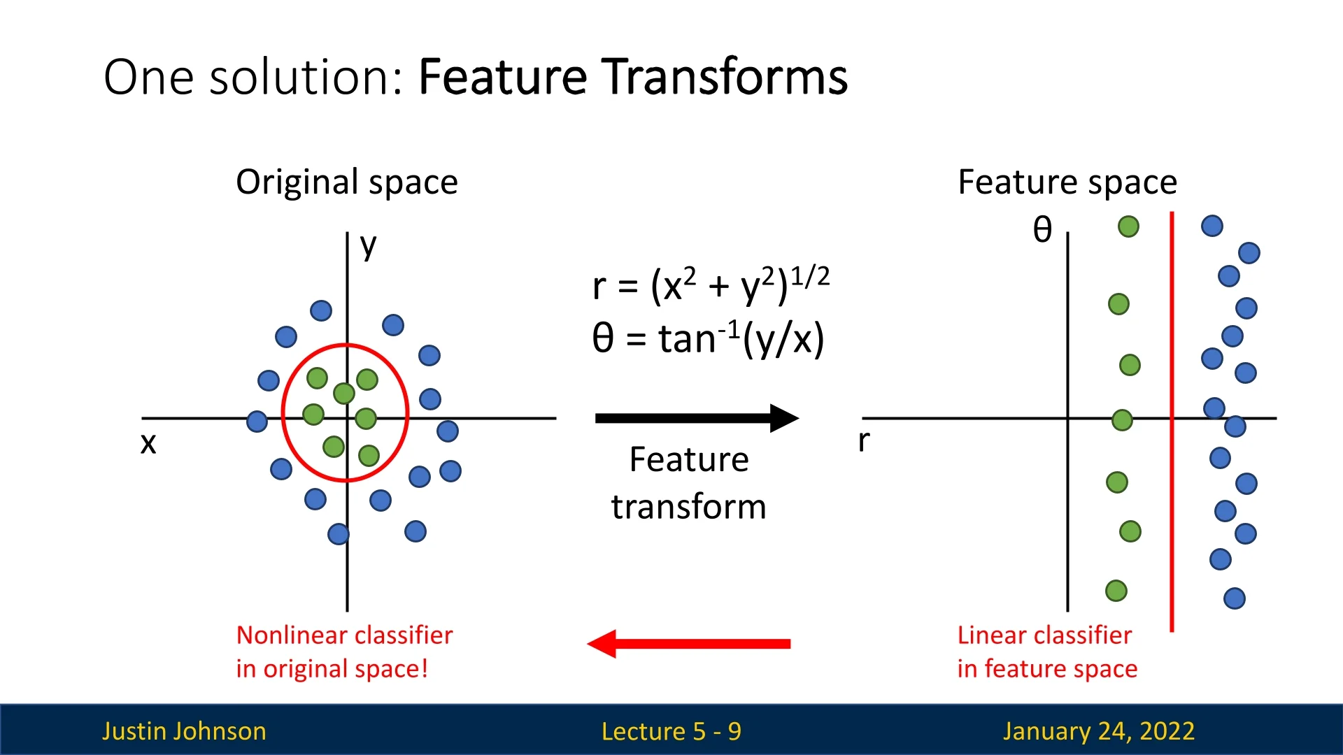
Figure 5.1: Cartesian to polar transformation enabling linear separability in the feature space. -
Color Histogram: This transformation is useful in computer vision. The RGB spectrum is divided into discrete bins, and each pixel is assigned to a corresponding bin, creating a histogram that captures the overall color distribution in the image. This approach removes spatial information, which can be helpful when objects consistently exhibit certain colors but may appear in different parts of the image.
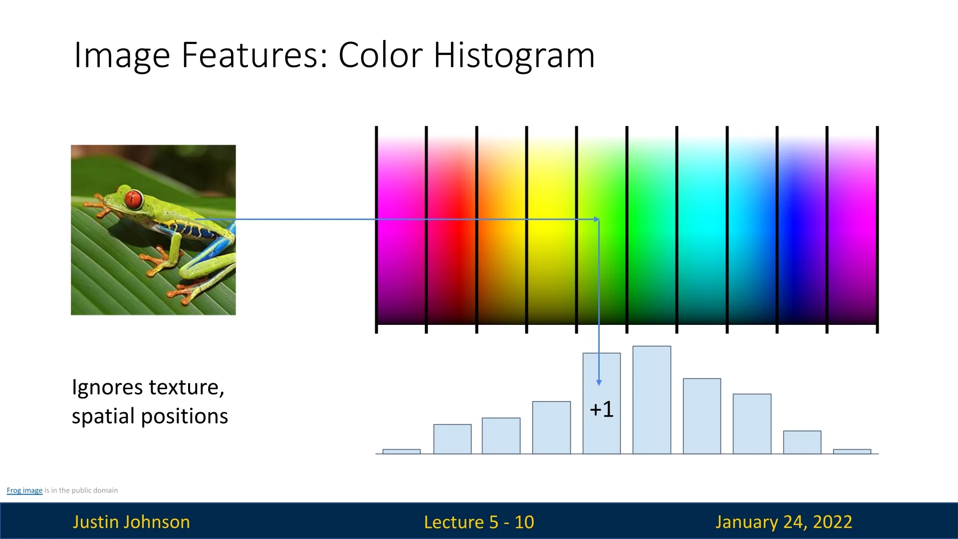
Figure 5.2: Color histogram as a feature representation for images. In such cases, this approach works well. A good example provided in the lecture (5.2) is the one of a class of red frogs that are always seen on a green background. However, the color histogram transformation fails in terms of classification when spatial structure is critical for the task, or when there are great color similarities across different categories.
-
Histogram of Oriented Gradients (HoG): The HoG transformation removes color information and retains edge orientation and strength. This approach complements the color histogram by focusing on local structure instead of overall color. It has been widely used in computer vision tasks, particularly for object detection, up to the mid-to-late 2000s.
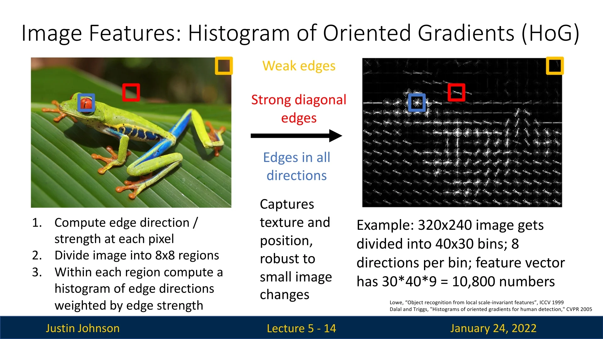
Figure 5.3: Histogram of Oriented Gradients (HoG) as a feature representation for images.
5.1.3 Challenges in Manual Feature Transformations
While feature transforms like color histograms and HoG are effective, they have significant limitations:
- They require practitioners to define specific rules for feature extraction, which can be time-consuming and error-prone.
- These hand-crafted features may not generalize well to real-world datasets, especially for out-of-distribution examples or uncommon instances (e.g., a frog of an unusual color or a cat without whiskers).
5.1.4 Data-Driven Feature Transformations
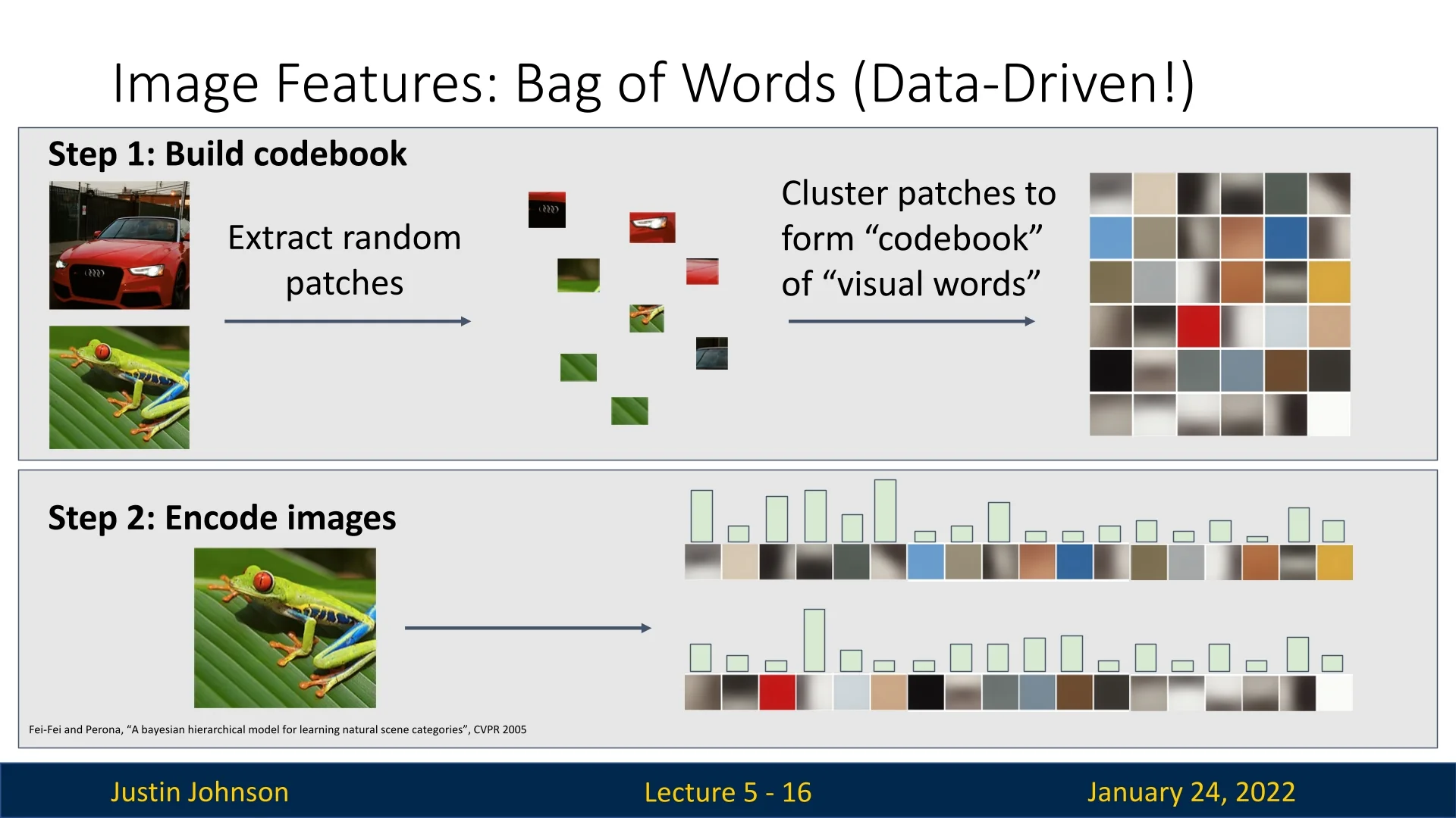
Unlike manual transformations, data-driven methods automatically derive features from the dataset, reducing the reliance on domain expertise. One such example is the Bag of Words approach.
The approach works as follows:
- Random patches are extracted from training images and clustered to form a codebook of ”visual words”.
- For each input image, a histogram is created to count how often each visual word appears.
- This method captures common structures and patterns in the dataset without requiring manual feature specification.
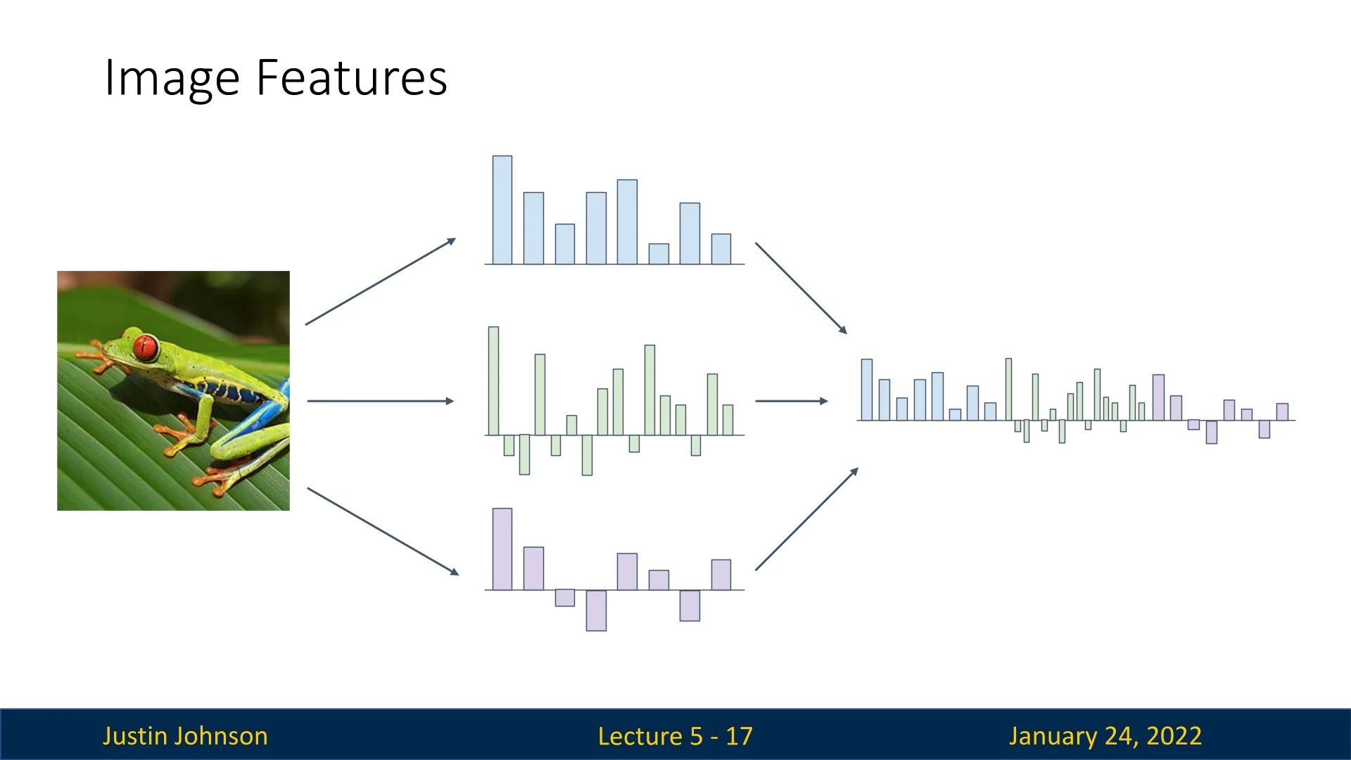
5.1.5 Combining Multiple Representations
Features derived from different transformations can be concatenated into a single high-dimensional feature vector. This combination allows capturing complementary aspects of the data (e.g., color, texture, and edges) for more robust classification. In the lecture Justin demonstrated this approach by combining color histogram, HoG and ’Bag of Visual Words’ we’ve covered earlier into a single concatenated representation vector.
5.1.6 Real-World Example: 2011 ImageNet Winner
Before the advent of deep learning, this approach of combining feature representations was considered state-of-the-art. The winner of the 2011 ImageNet Classification Challenge employed a sophisticated pipeline:
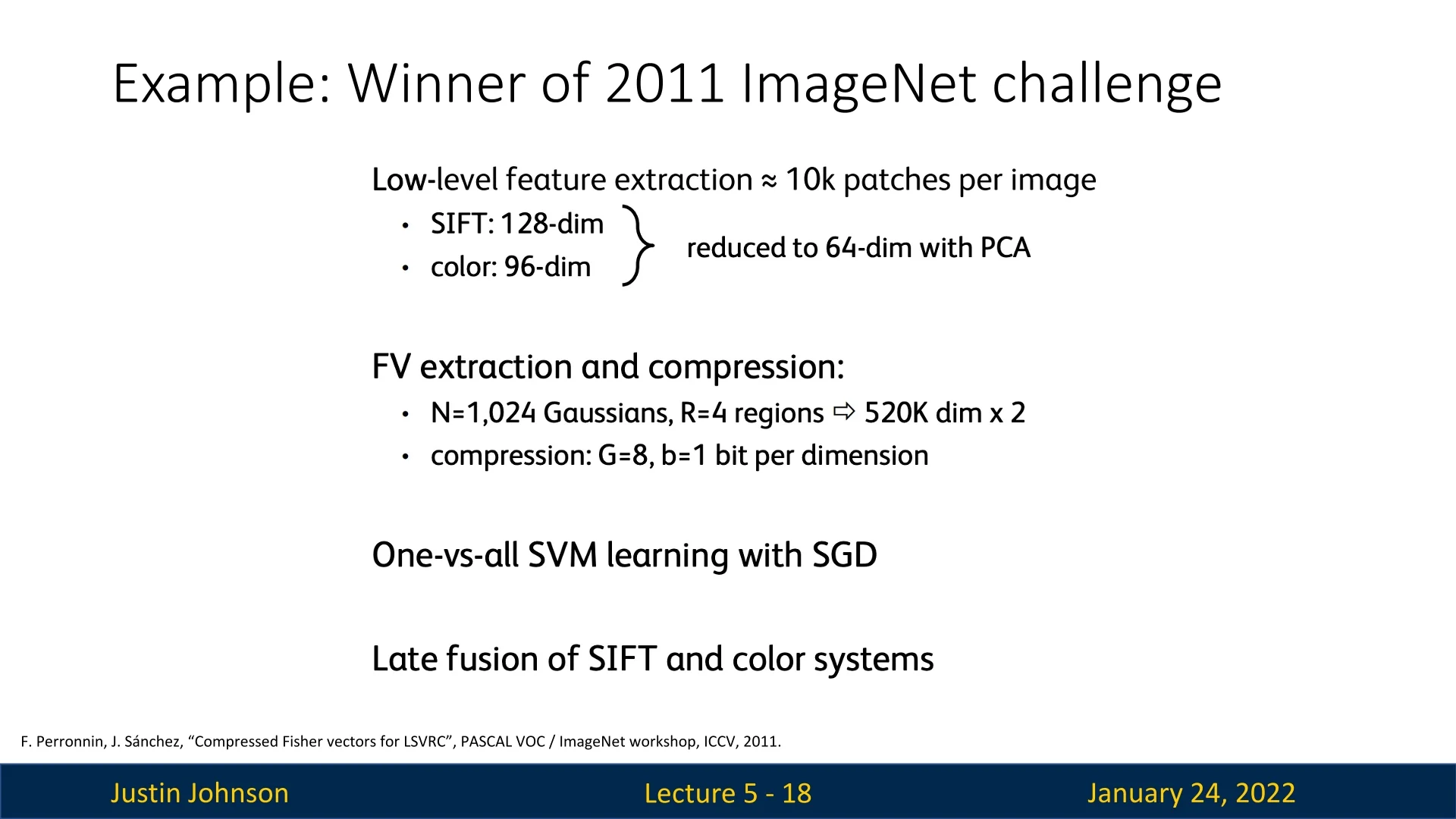
The pipeline included:
- 1.
- Extracting approximately 10,000 image patches per image, covering various scales, sizes, and locations.
- 2.
- Features like SIFT and color histograms were extracted, and dimensionality reduction was performed using PCA.
- 3.
- Fisher Vector feature encoding was applied to further compress and encode these features.
- 4.
- A one-vs-all Support Vector Machine (SVM) was trained on the resulting features for classification.
This approach highlights the complexity and manual effort involved in feature engineering before the rise of deep learning.
5.2 Neural Networks: The Basics
5.2.1 Motivation for Neural Networks
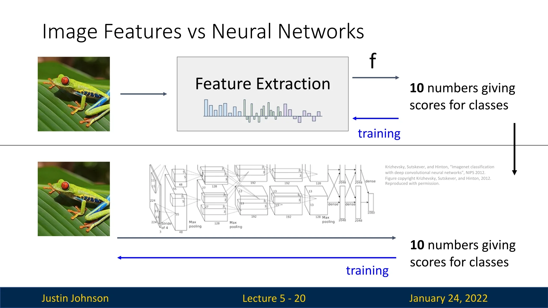
Despite their effectiveness in specific scenarios, feature transforms face inherent limitations due to their reliance on manual design or pre-specified transformations. Neural networks overcome these limitations by jointly learning feature representations and classification models in an end-to-end framework, as we will explore in the next sections.
When building a linear classifier on top of the features extracted through the methods discussed earlier, we are only tuning the parameters of the classifier (the final component in the pipeline) to maximize classification performance. This approach is limited because it fixes the feature extraction stage and optimizes only the classifier. Instead, we want an end-to-end pipeline where every component, from feature extraction to classification, is fully tunable during training based on the data. This is one of the primary motivations for switching to neural networks.
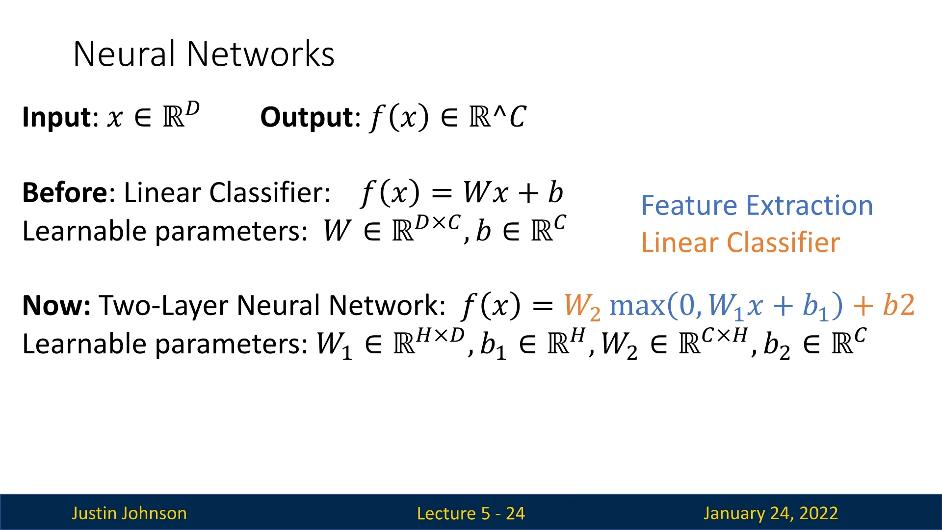
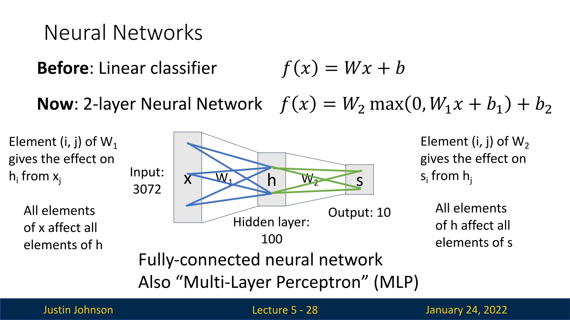
A small neural network, in its functional form, is quite similar to a linear classifier. The key difference is the introduction of a non-linear function applied to the result of the vector-matrix multiplication (between the input vector and the weight matrix). This 2-layer neural network can be generalized to any desired number of layers. Layers other than the input and output layers are called hidden layers, and deep neural networks can have an arbitrary number of them.
5.2.2 Fully Connected Networks
A fully connected neural network, also known as a multi-layer perceptron (MLP), is structured so that every neuron in one layer is connected to every neuron in the next layer. In practical terms, this means each neuron in the next layer receives inputs from all neurons in the current layer, each with its own learnable weight. This dense connectivity can capture complex relationships but often requires a large number of parameters.
5.2.3 Interpreting Neural Networks
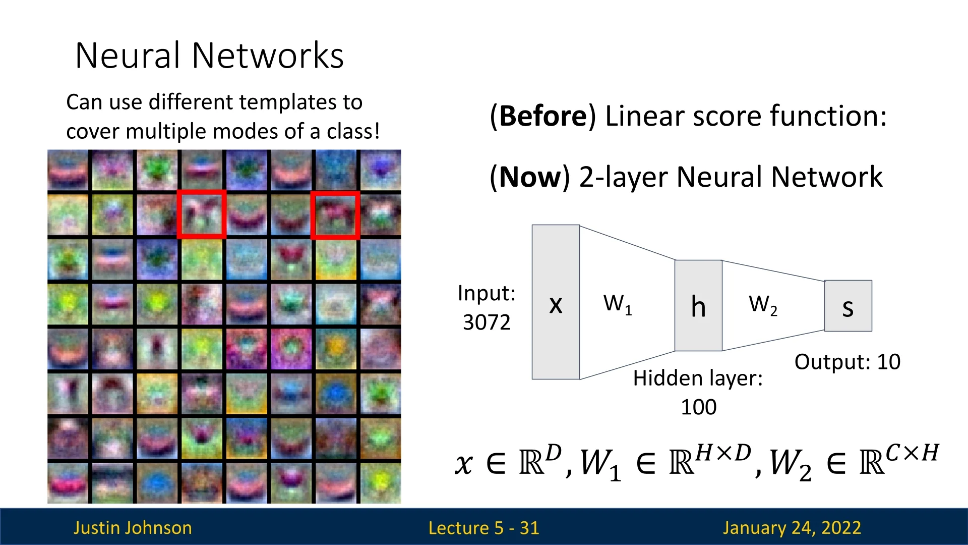
Neural networks can be analyzed in a way similar to linear classifiers. For instance, the weight matrix \(\mathbf {W}_1\) in the first layer can be reshaped and visualized as templates, each indicating how strongly it responds to particular spatial patterns in the input image. While many of these templates are not immediately interpretable, some do reveal recognizable structures.
A notable example discussed in the lecture involves two “horse” templates: one for a left-facing horse and another for a right-facing horse. This arrangement avoids the “double-headed horse” phenomenon seen in some linear classifiers, where a single template tries to capture multiple orientations or modes of an object class.
In the second layer of the network, these template responses are recombined (via another set of weights) to perform classification. Because distinct templates can be linearly combined to form more complex features, the network is said to learn a distributed representation. In other words, while individual templates may be non-intuitive or partially interpretable, their collective combination yields rich, discriminative features for tasks like object recognition.
Network Pruning: Pruning Redundant Representations One challenge in neural networks is redundancy, where multiple filters or features learn the same thing. A technique called network pruning addresses this issue. In this approach, a large neural network is trained, and as a post-processing step, redundant representations are pruned to simplify the network without significantly affecting its performance.
5.3 Building Neural Networks
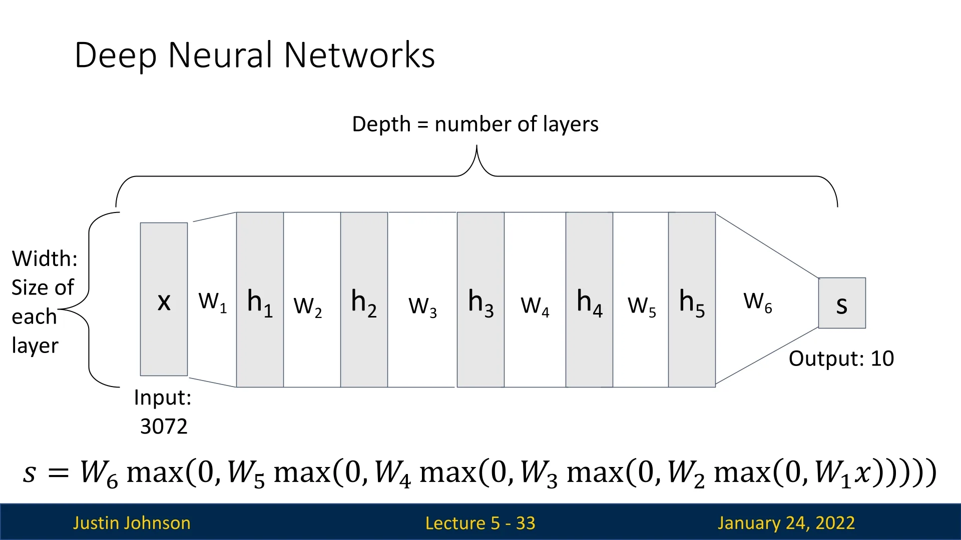
Neural networks are formed by stacking multiple layers. The depth of a network refers to the number of these layers, while the width describes the number of neurons (hidden units) per layer.
5.3.1 Activation Functions: Non-Linear Bridges Between Layers
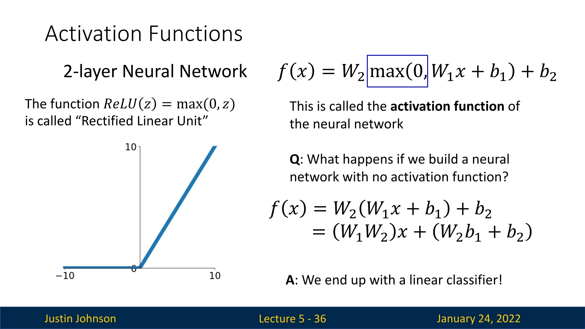
A crucial component that distinguishes neural networks from linear classifiers is the activation function. After computing \[ h = \mathbf {W} \mathbf {x} + \mathbf {b}, \] the network applies a non-linear function \( f(h) \). This combination of a linear transformation followed by a non-linear activation enables the network to model complex, non-linear decision boundaries.
Without non-linearities (e.g., if you simply had \(\mathbf {W}_2 (\mathbf {W}_1 \mathbf {x})\)), the combined transformation would still be linear, reducing the model’s expressiveness to that of a single matrix multiplication. This is illustrated in the figure below, where collapsing multiple linear layers into one (\(\mathbf {W}_3 = \mathbf {W}_2 \mathbf {W}_1\)) reduces the network to a linear classifier.
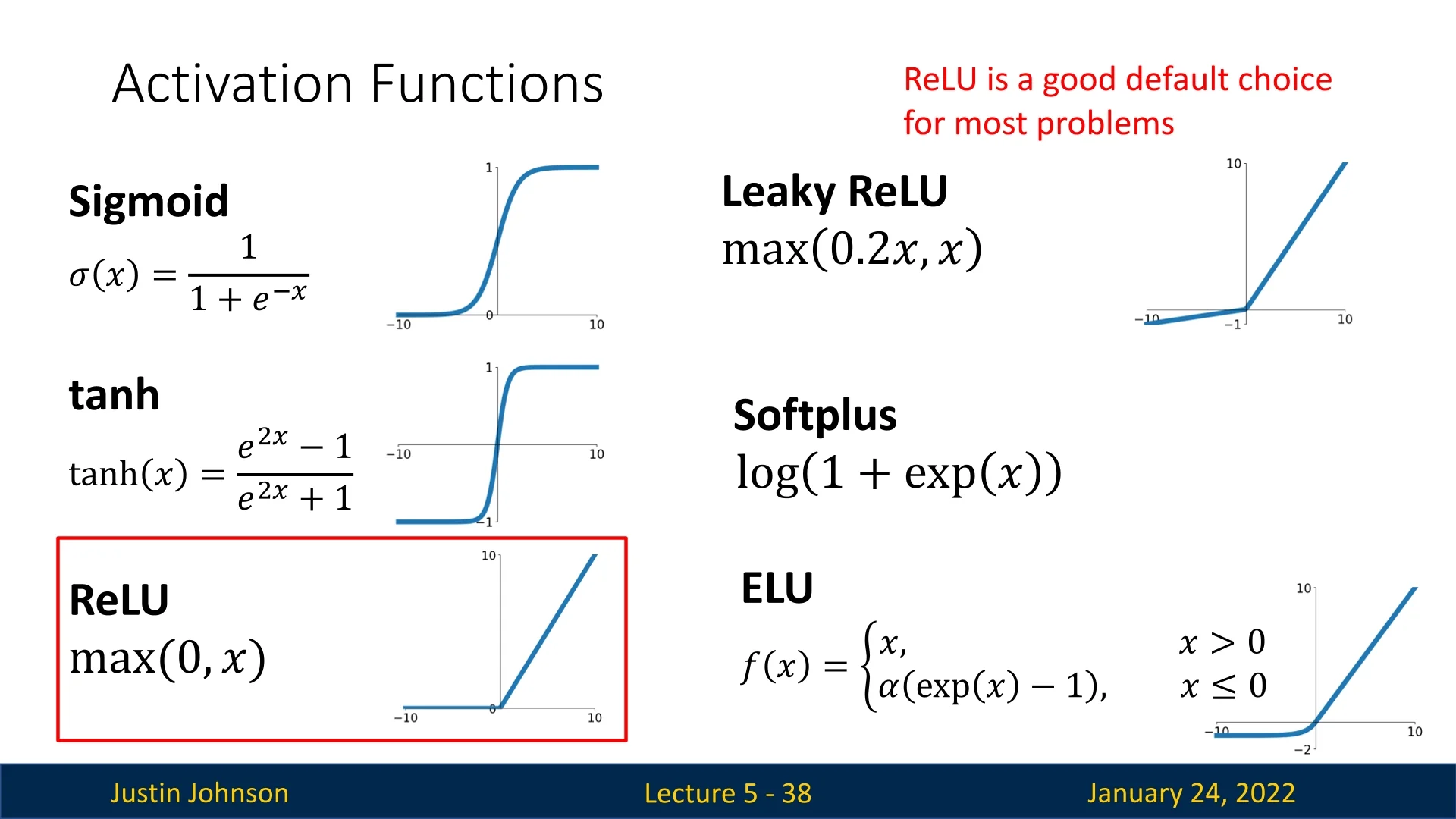
Why Non-Linearity Matters Non-linear activation functions grant neural networks the universal approximation property, enabling them to represent virtually any function given sufficient capacity (enough parameters and layers). Common activation functions include:
- ReLU (\(\max (0, x)\)): A popular choice due to its simplicity and ability to mitigate vanishing gradients. Works effectively in most modern architectures.
- Sigmoid (\(\sigma (x)\)): Historically significant but less common now due to issues such as vanishing gradients for large positive or negative inputs.
- Tanh, Leaky ReLU, and other variants: Offer different trade-offs regarding smoothness, gradient flow, and negative-domain behavior.
The figure below highlights these activation functions. Historically, Sigmoid was widely used but has largely been replaced by ReLU, which has become the de facto standard, similar to how Adam dominates optimizers.
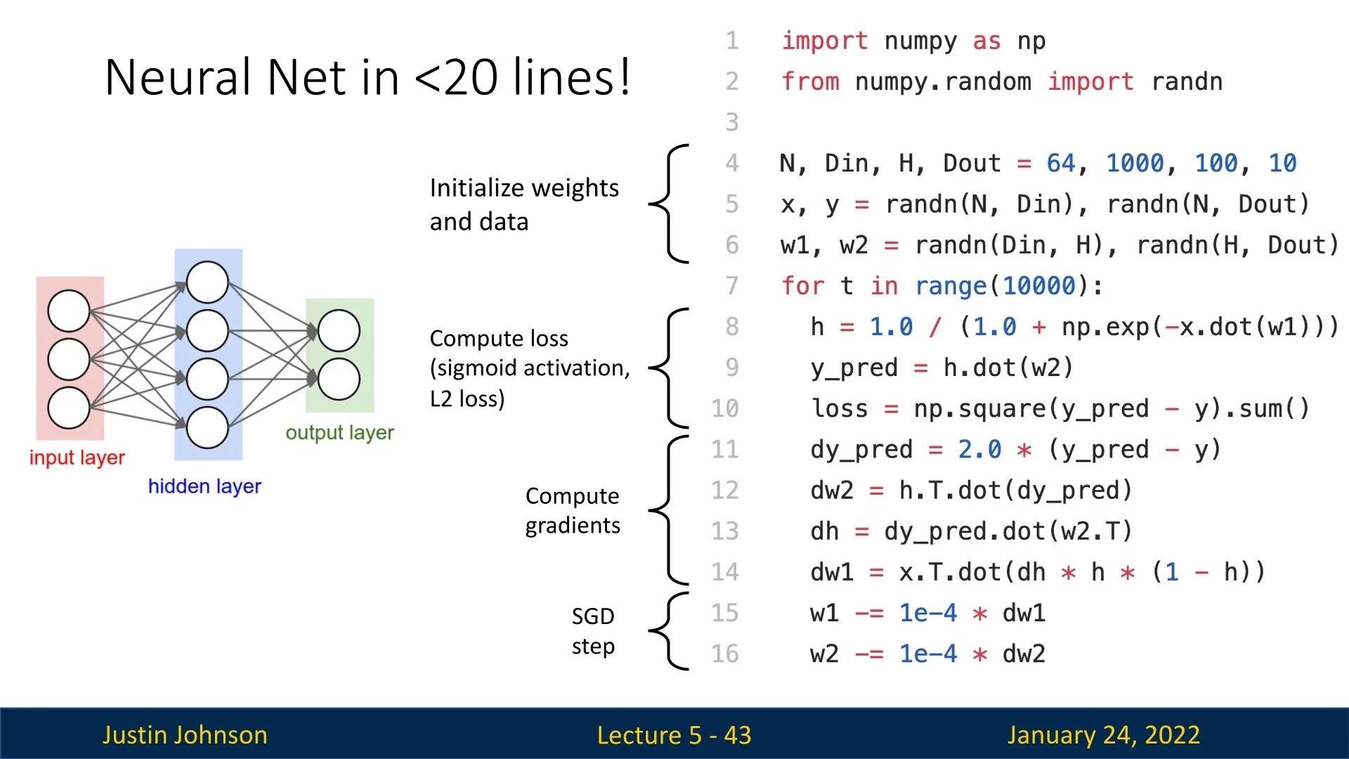
5.3.2 A Simple Neural Network in 20 Lines
Despite their conceptual depth, neural networks can be implemented succinctly. Below is an example of a minimal NumPy implementation of a neural network with:
- An input layer.
- One hidden layer with an activation function (e.g., ReLU).
- An output layer for classification or regression.
The following figure demonstrates this simplicity, showcasing the essential ingredients of a feedforward neural network.
5.4 Biological Inspiration
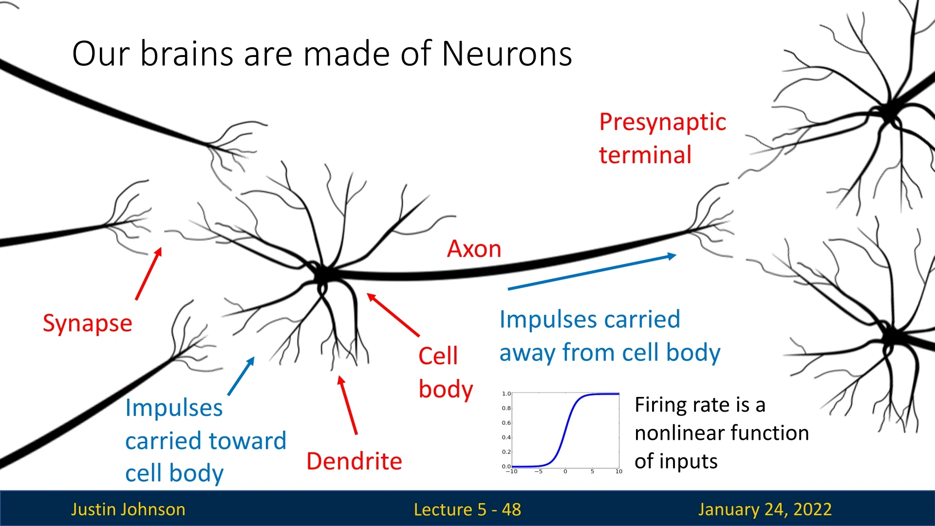
The term neural network draws loose inspiration from the structure of the human brain. Biological neurons consist of:
- Dendrites: Collect incoming signals.
- Cell Body: Sums and processes the signals.
- Axon: Transmits signals away from the cell body.
- Synapses: Modulate signal strength at neuron junctions.
The flow of impulses is illustrated below, where the cell body processes inputs and sends output signals through the axon.
5.4.1 Biological Analogy: a Loose Analogy
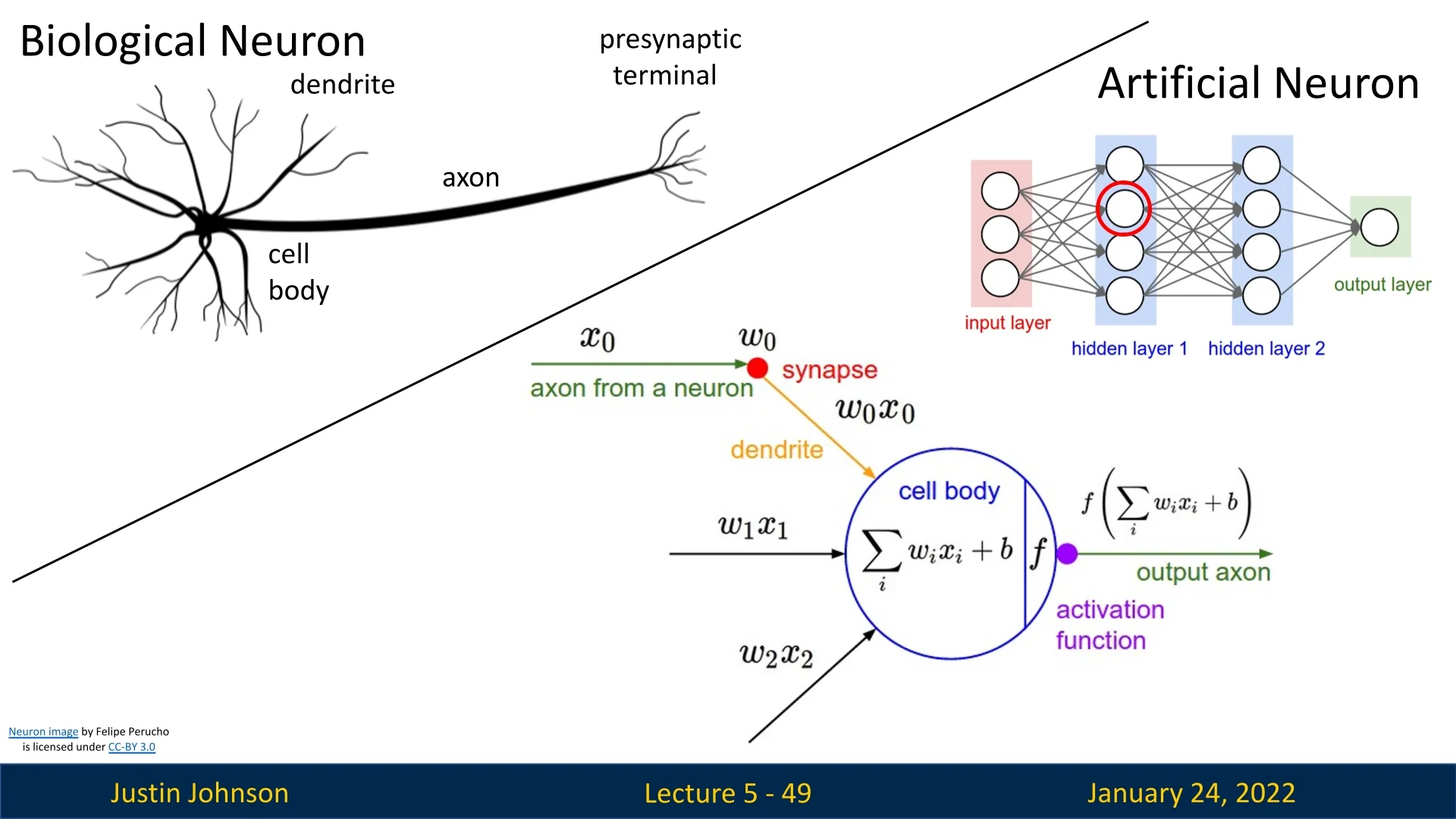
While neural networks borrow terminology and broad conceptual inspiration from neuroscience, the actual mechanisms differ significantly:
- Connectivity Patterns: Biological neurons form complex, recurrent, and varied circuits, while artificial networks often use structured, layer-based designs.
- Weights vs. Synapses: Artificial weights are scalar values updated via gradient descent, unlike the chemical and electrical processes in biological synapses.
- Dendritic Computation: Biological dendrites can perform non-linear operations before signals reach the cell body, while artificial neurons rely on simpler computations.
5.5 Space Warping: Another Motivation for Artificial Neural Networks
Neural networks provide a powerful approach to warp the input space into separable regions, enabling complex tasks like classification and regression. In the following parts, we will explore this concept of space warping and demonstrate how multi-layer architectures reshape the feature space to disentangle data distributions effectively.
Linear classifiers can be understood geometrically as operating in a high-dimensional input space, where each row of the weight matrix corresponds to a hyperplane dividing the space. These hyperplanes act as decision boundaries, and the dot product between the input and the weight matrix determines classification scores. Each hyperplane has a score of 0 along the boundary, increasing linearly as we move perpendicularly away from it.
Another perspective is to view the classifier as warping the input space. This involves transforming the input features \( x_1, x_2 \) into new coordinates \( h_1, h_2 \), based on the learned transformation \( h = \mathbf {W} \mathbf {x} \).
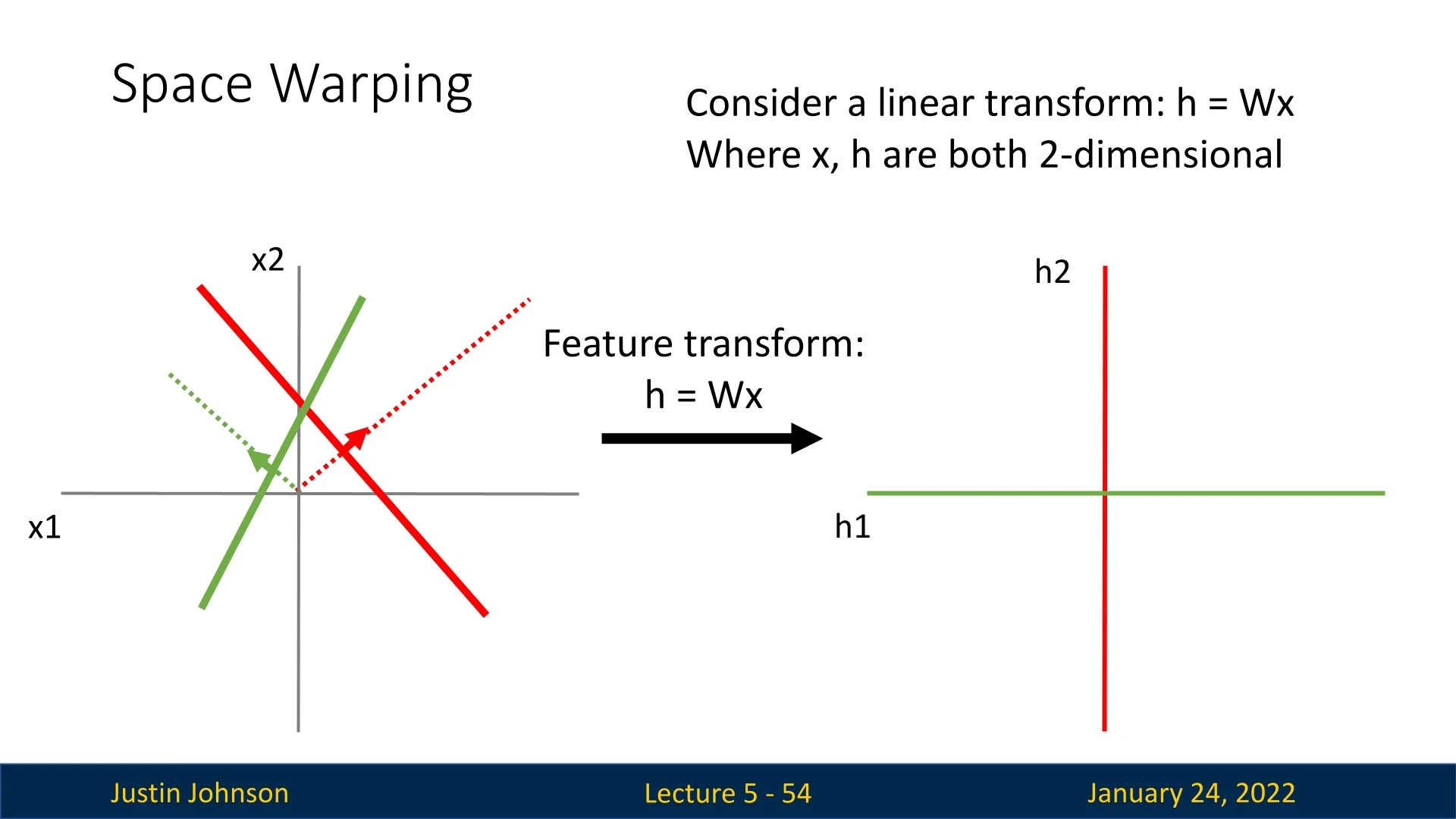
5.5.1 Linear Transformations and Their Limitations
With a linear transformation, the input space is linearly deformed. In the example below, two lines in the input space (representing decision boundaries) divide the space into four regions: A, B, C, and D.
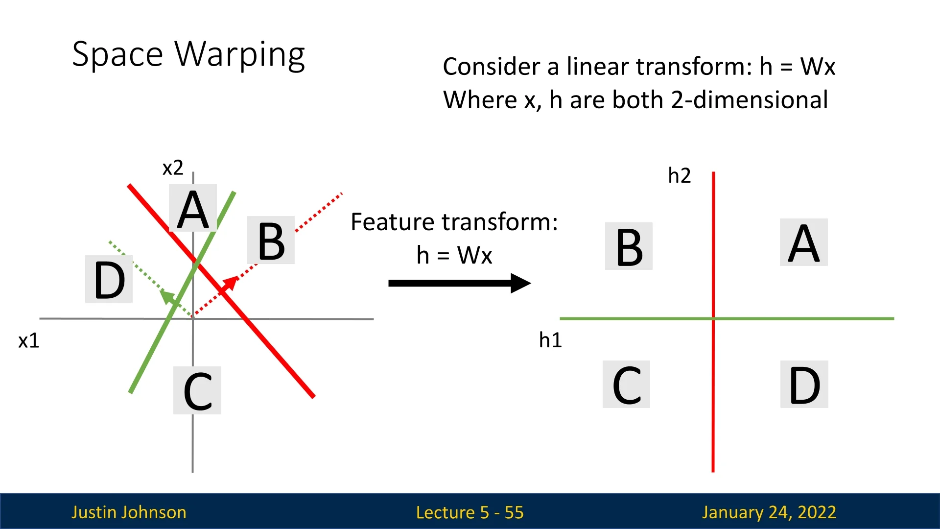
Each of these regions is transformed linearly into the new feature space. However, a critical limitation emerges: Data that is not linearly separable in the input space will remain non-linearly separable after a linear transformation. Training a classifier in this transformed space fails to resolve the separability issue.
5.5.2 Introducing Non-Linearity with ReLU
What happens if the transformation applied to the data is non-linear? Consider a neural network with a hidden layer applying the ReLU activation function: \[ h = \mbox{ReLU}(\mathbf {W} \mathbf {x}) = \max (0, \mathbf {W} \mathbf {x}), \] where \( x \) and \( h \) are 2-dimensional vectors, and biases are ignored for simplicity.
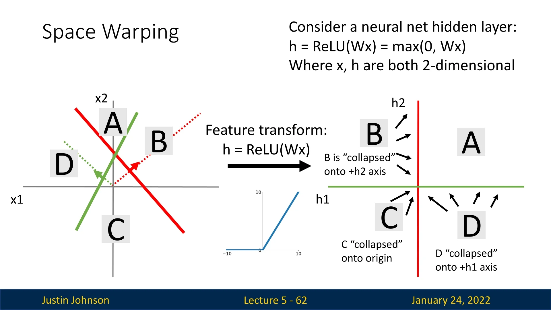
In this case:
- Quadrant A is transformed linearly.
- Quadrant B corresponds to a positive value for one feature (red) and a negative value for the other (green). ReLU collapses it onto the \( +h_2 \)-axis, setting the negative feature to 0.
- Quadrant D is similarly collapsed onto the \( +h_1 \)-axis.
- Quadrant C is entirely collapsed onto the origin, as both features are negative.
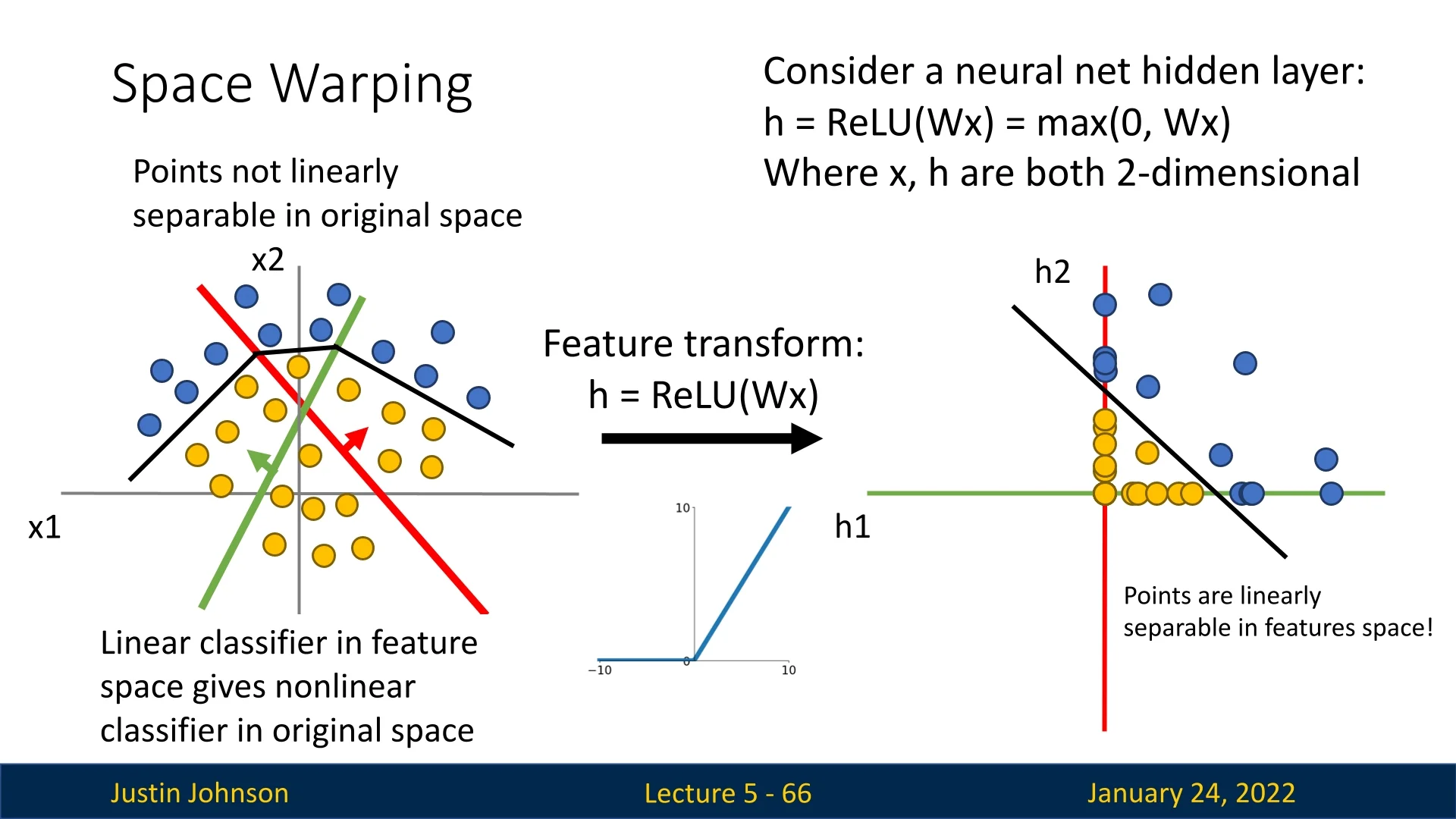
5.5.3 Making Data Linearly Separable
5.5.4 Scaling Up: Increasing Representation Power
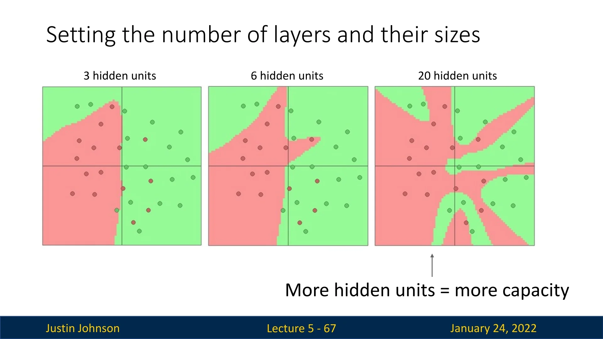
In this example, the neural network hidden layer had two dimensions, allowing it to fold the input space twice. By increasing the number of hidden units, the network gains the capacity to represent increasingly complex transformations. This results in more intricate decision boundaries in the original input space.
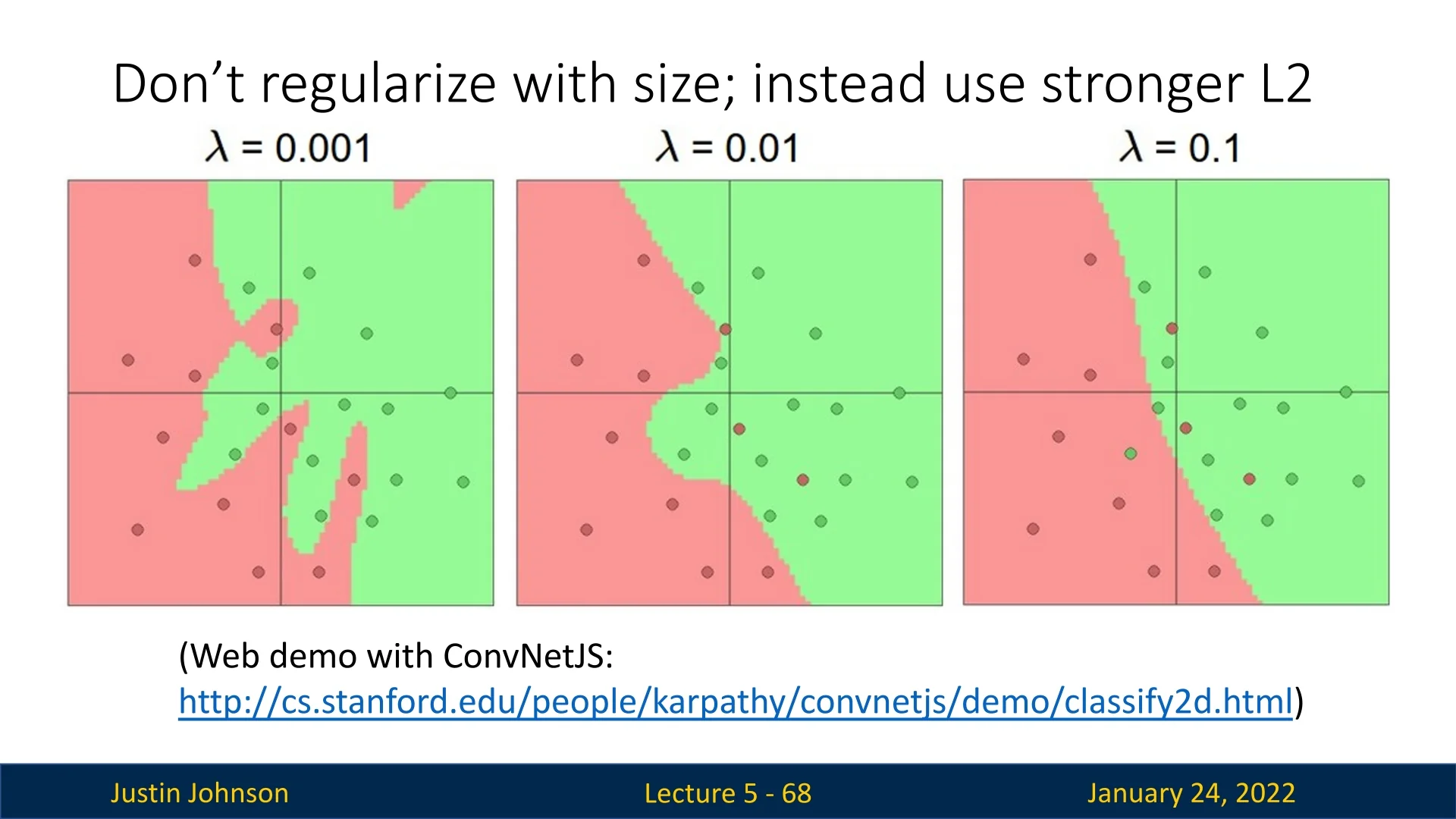
5.5.5 Regularizing Neural Networks
While increasing hidden units enhances the network’s representational capacity, care must be taken to avoid overfitting. Instead of limiting the number of neurons of hidden layers, stronger L2 regularization can be applied to smooth decision boundaries without altering the architecture.
5.6 Universal Approximation Theorem
The concept of neural networks as feature space transformers demonstrates their potential to learn very complex decision boundaries, vastly surpassing the capabilities of linear classifiers. Now we’ll formalize this power by introducing the concept of ’Universal Approximation’, which explores the types of functions neural networks can learn and their theoretical limitations.
The Universal Approximation Theorem states that a neural network with just one hidden layer can approximate any function \( f: \mathbb {R}^N \to \mathbb {R}^M \) to arbitrary precision, given certain conditions. These conditions include:
- The input space must be a compact subset of \( \mathbb {R}^N \).
- The function must be continuous.
- The term “arbitrary precision” requires formal definition.
While this result is mathematically profound, we will not delve into all these mathematical conditions behind it, as it is beyond the scope of this course. What we’ll try to do is focus on the practical side, building a method that can be used to construct any given function based on neural networks.
5.6.1 Practical Context: The Bump Function
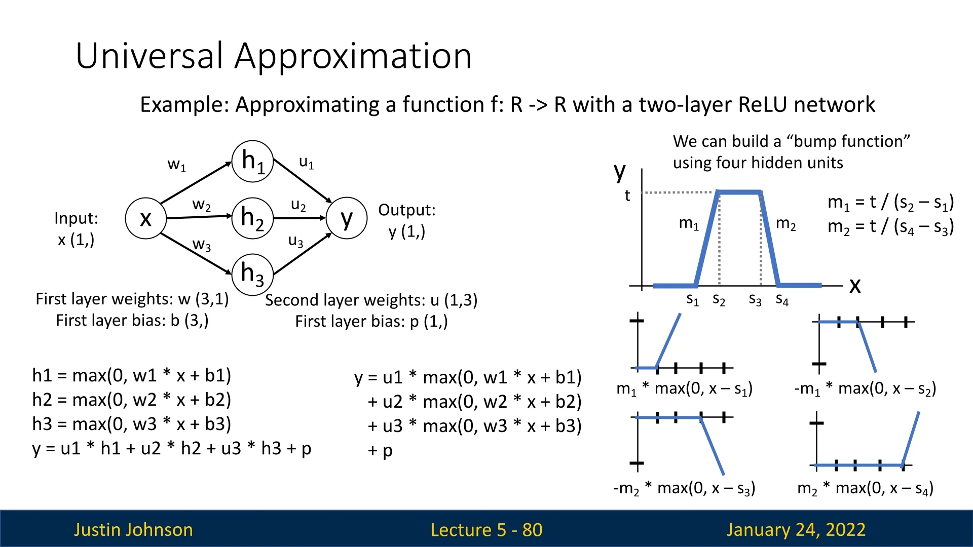
A concrete illustration of the universal approximation theorem is the construction of a simple bump function using a small two-layer ReLU network. This example demonstrates how even a few ReLU units can be combined to synthesize localized, non-linear patterns—showing how neural networks can approximate arbitrary continuous functions through composition.
Constructing a Bump with ReLU Units Consider a one-dimensional input \( x \) passed through four hidden ReLU activations: \[ h_i(x) = \max (0, w_i x + b_i), \quad i = 1, 2, 3, 4, \] whose outputs are linearly combined to form: \[ y = \sum _{i=1}^{4} u_i h_i(x) + p. \] Each ReLU creates a hinge-shaped piecewise-linear segment that becomes active (nonzero) only when \( x > -b_i / w_i \). By carefully setting the weights \( w_i, b_i, u_i \), we can align the breakpoints of these hinges at four positions \( s_1, s_2, s_3, s_4 \) along the \(x\)-axis, and choose slopes \(m_1, m_2\) such that: \[ m_1 = \frac {t}{s_2 - s_1}, \qquad m_2 = \frac {t}{s_4 - s_3}. \] These parameters generate a flat baseline, a linear rise to height \(t\), a plateau, and then a symmetric linear fall—together forming a smooth “bump” localized between \(s_1\) and \(s_4\).
Why the Bump Matters This bump construction is fundamental because it serves as a local building block for more complex approximations. By summing multiple such bumps, each positioned and scaled differently, we can approximate any continuous function on a bounded domain: \[ f(x) \approx \sum _{k=1}^{K} a_k \, \mbox{bump}_k(x), \] where each \(\mbox{bump}_k(x)\) is formed using four ReLU units. With \(4K\) hidden units, the network can represent \(K\) independent bumps—each capturing a local feature of the target function. As \(K\) increases, the approximation becomes increasingly accurate.
Intuitive Understanding Each bump acts like a localized basis function, similar to how sine waves in Fourier analysis or Gaussians in radial basis networks capture local structure. ReLU networks, therefore, build complex functions by stitching together many such simple, overlapping pieces. This demonstrates a key insight of universal approximation: even shallow networks, given enough hidden units, can approximate arbitrarily complex continuous mappings through a sum of locally linear “bump” functions.
In essence: Each ReLU adds a hinge to the function; combining several hinges creates a bump; and combining many bumps creates an arbitrary continuous curve—the essence of deep learning’s expressive power.
5.6.2 Questions for Further Exploration
This proof of capacity raises several interesting questions:
- What about the gaps between the bumps?
- Can similar results be achieved with other activation functions?
- How does this extend to higher-dimensional inputs and outputs?
For those interested in a deeper dive, Michael Nielsen’s book, Chapter 4 explores these concepts in detail1.
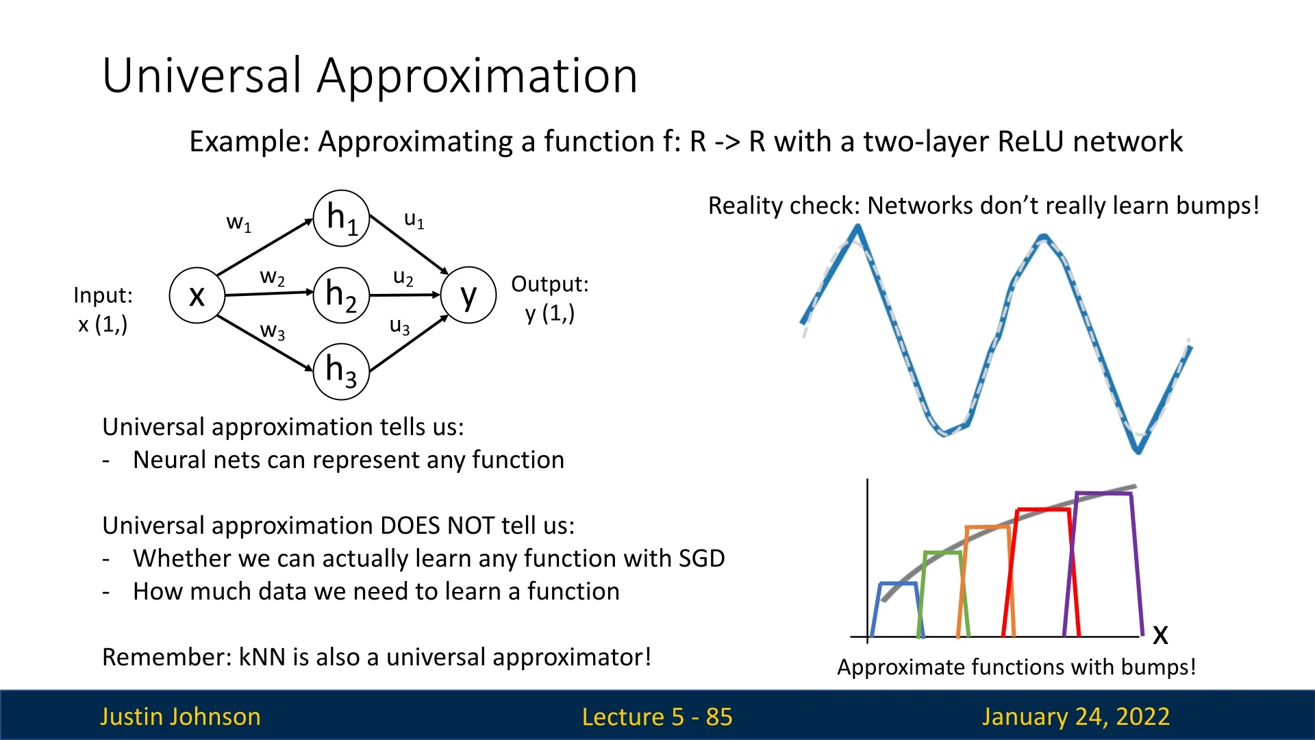
5.6.3 Reality Check: Universal Approximation is Not Enough
While the Universal Approximation Theorem demonstrates the capacity of neural networks to represent any function, practical training dynamics differ significantly. When training with stochastic gradient descent (SGD), neural networks do not learn these bump functions explicitly.
The theorem does not address:
- How effectively functions can be learned using gradient-based methods,
- How much data is required for effective learning,
- Practical considerations like optimization challenges and generalization.
As a comparison, \( k \)-Nearest Neighbors (kNN) is also a universal approximator, but this property alone does not make it the best model for most tasks. Universal approximation, while a nice property, is insufficient to declare neural networks superior.
Enrichment 5.6.4: Deep Networks vs Shallow Networks
A neural network with one hidden layer is theoretically sufficient to approximate any continuous function. This result highlights the expressive power of even shallow networks but does not imply practical feasibility.
A natural question arises: Why not simply use one deep layer? In other words, why not train only shallow networks to solve our desired tasks? There are several reasons why this is impractical:
- Memorization vs. Generalization: Shallow networks can memorize training data effectively but empirically often fail to generalize well to unseen data.
- Scalability Issues: While a single hidden layer can approximate any function, the required number of neurons grows exponentially with task complexity. More formally, for a function that requires a depth-\(D\) network with width \(W\), a depth-1 network may require width up to \(O(W^D)\) [143, 634]. This exponential growth makes training infeasible as the number of parameters and computations explode.
- Feature Hierarchies and Representation Learning: Deeper networks naturally learn hierarchical representations, where each layer extracts increasingly abstract features [36]. Mathematically, many real-world functions are compositional in nature, meaning they can be expressed as a composition of simpler functions: \begin {equation} f(x) = f_L \circ f_{L-1} \circ \dots \circ f_1(x). \end {equation} A deep network explicitly models this hierarchical structure, making it exponentially more efficient than a shallow network in terms of representation capacity [497].
Enrichment 5.6.4.1: Why Not Just Use a Very Deep and Wide Network?
While deep networks improve representation learning, increasing depth and width comes with trade-offs:
- Overfitting: More parameters increase the risk of overfitting, particularly in low-data regimes.
- Computational Costs: Training deeper networks requires longer runtimes and significantly more memory, particularly as backpropagation scales linearly with depth.
- Optimization Challenges: Deep networks suffer from vanishing and exploding gradients due to repeated matrix multiplications, making them harder to train [236, 485].
Hence, while a single hidden layer is sufficient in theory, deeper networks provide better generalization, improved representation learning, and computational efficiency in practice. The choice of depth and width remains a crucial consideration, balancing expressivity, generalization, and computational cost.
5.7 Convex Functions: A Special Case
Convex functions exhibit desirable properties for optimization.
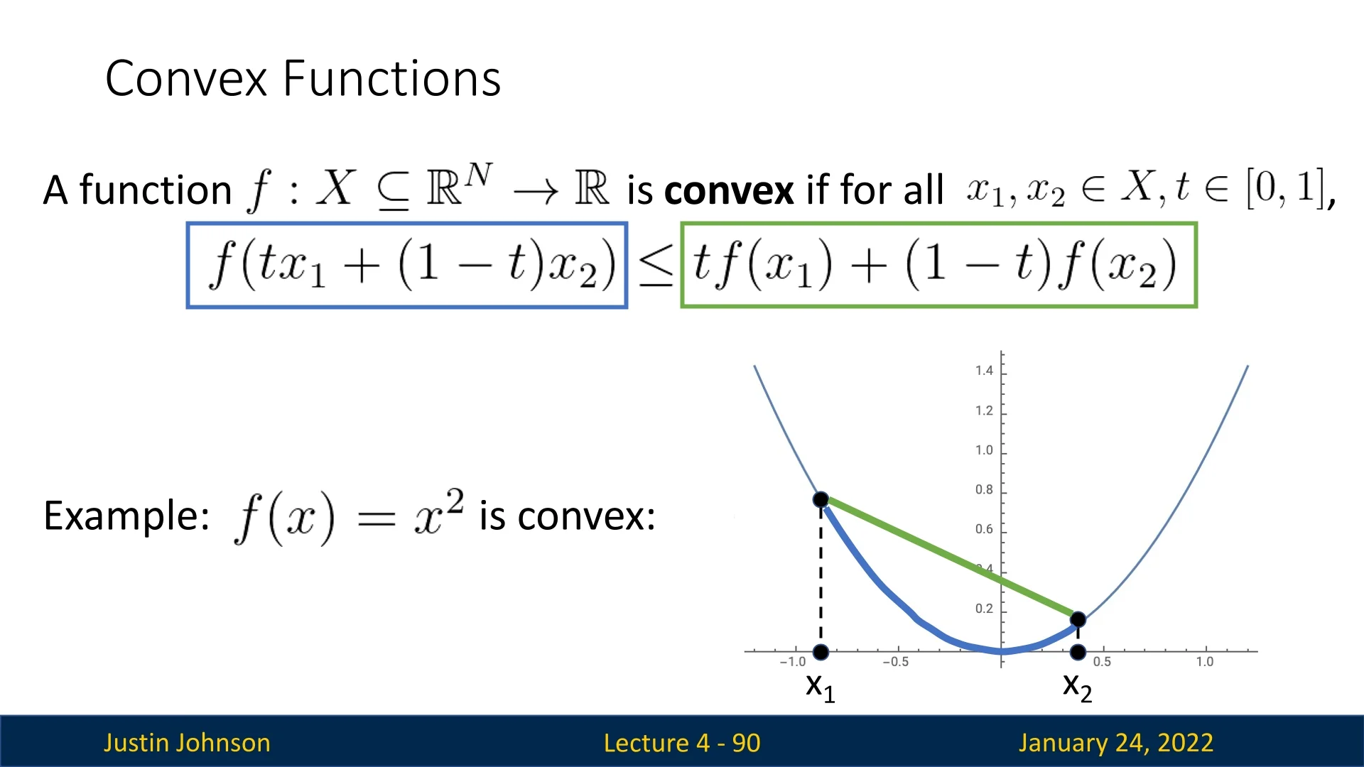
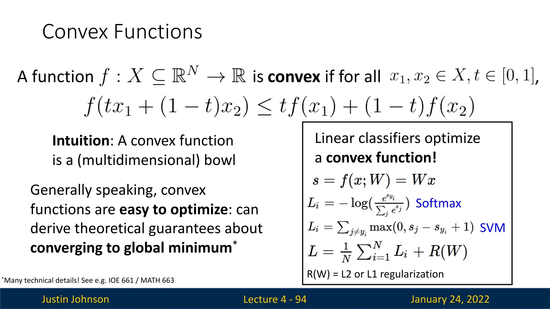
Intuitively, convex functions resemble multidimensional bowls. They are defined as functions \( f \) such that: \[ f(\alpha x_1 + (1 - \alpha ) x_2) \leq \alpha f(x_1) + (1 - \alpha ) f(x_2), \quad \forall \alpha \in [0, 1]. \]
This property ensures:
- The local minimum of a convex function is also its global minimum.
- Theoretical guarantees exist for convergence to the global minimum.
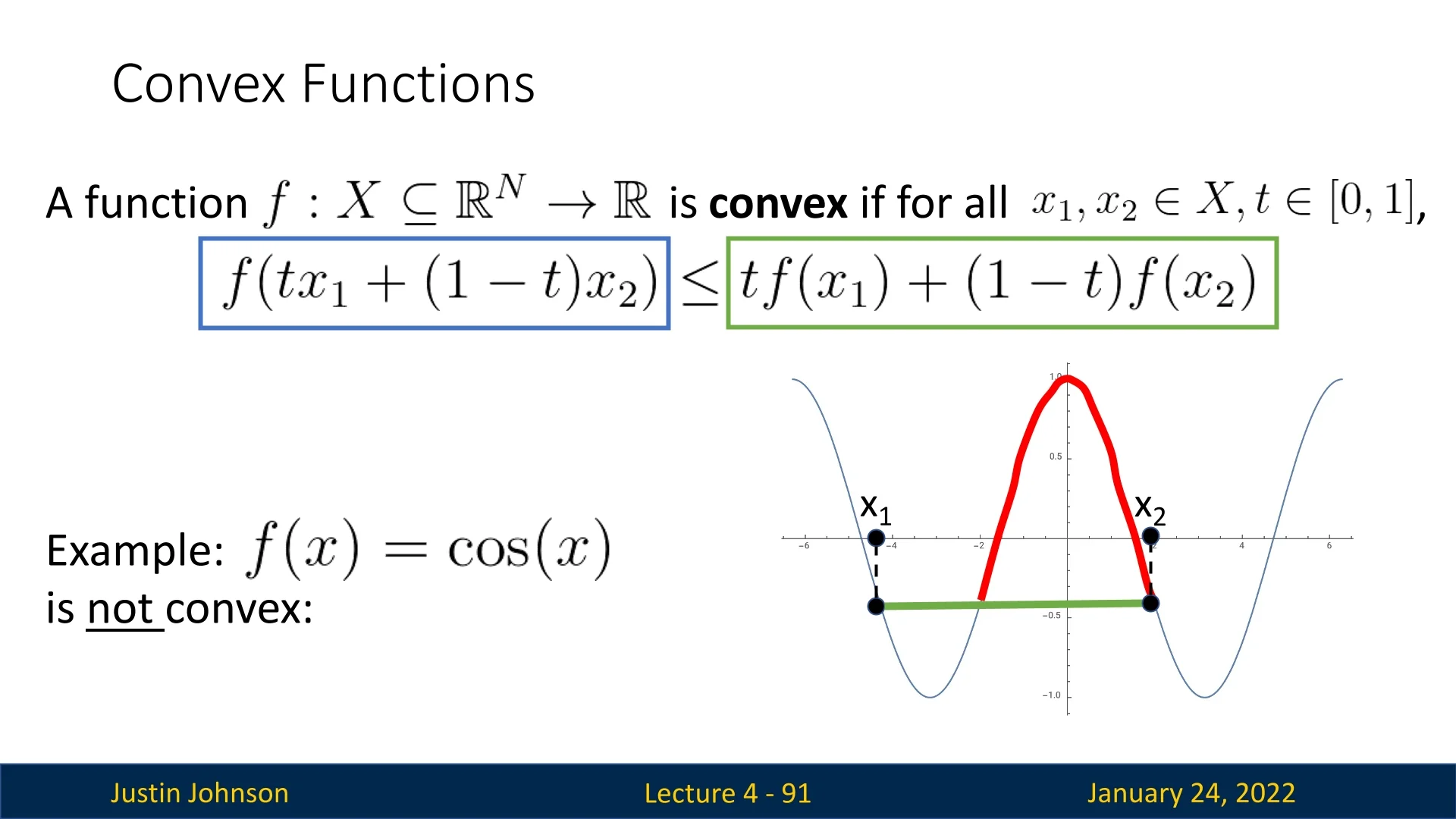
5.7.1 Non-Convex Functions
In contrast, functions like \( f(x) = \cos (x) \) are non-convex, as there exist secant lines between two points that lie below the function itself.
5.7.2 Convex Optimization in Linear Classifiers
The optimization problems arising from linear classifiers, such as those using the softmax or SVM loss functions, are convex due to their mathematical formulation. Convexity arises from the following properties:
- Convex Loss Functions: The softmax and SVM losses are convex functions of their input scores. For example, the negative log-likelihood loss used in softmax is convex because the log-sum-exp function (involved in the computation) is convex.
- Linear Transformations of Input Features: Linear classifiers involve a dot product between the input feature vector \( \mathbf {x} \) and the weight vector \( \mathbf {w} \). As linear transformations preserve convexity, the overall objective function remains convex.
- No Hidden Layers: Linear classifiers lack non-linear components or hidden layers, which are typical sources of non-convexity in neural networks.
This convex nature ensures:
- The optimization process is robust and less sensitive to initialization since the loss surface does not contain local minima or saddle points.
- Convergence to the global minimum is guaranteed under appropriate conditions, such as when using gradient descent with a suitable learning rate.
5.7.3 Challenges with Neural Networks
In contrast, optimization problems for neural networks are inherently non-convex. This means:
- There are no guarantees of convergence to a global minimum.
- Empirical success often relies on heuristics, such as good initialization, proper learning rates, and regularization techniques.
Despite this theoretical limitation, neural networks perform well empirically, which remains a topic of active research.
5.7.4 Bridging to Backpropagation: Efficient Gradient Computation
In this chapter, we explored the immense power of neural networks, from their ability to approximate complex functions to their optimization challenges. While gradient-based optimization techniques like SGD and its variants are essential for training deep neural networks, a critical question remains: how can we compute gradients efficiently for such complex architectures?
Deep neural networks often consist of millions or billions of parameters across multiple layers, making direct gradient computation infeasible using naive methods like numeric differentiation. For these models to be trainable at scale, we require a systematic and efficient way to compute the gradients of the loss function with respect to every parameter in the network.
This is where the backpropagation algorithm comes into play. Backpropagation leverages the chain rule from calculus to propagate gradient information layer by layer, drastically reducing the computational cost of gradient evaluation. It ensures that the gradient of the loss with respect to each parameter is computed in a time-efficient manner, even for networks with a deep and complex structure.
In the next chapter, we will delve into the mathematical foundations and mechanics of backpropagation, illustrating how it enables the training of neural networks at the scale required for modern applications.
1Nielsen, Michael A. Neural Networks and Deep Learning, Determination Press, 2015. Available online at http://neuralnetworksanddeeplearning.com/.