Lecture 14: Object Detectors
14.1 Beyond R-CNN: Advancing Object Detection
In the previous chapter we focused on what object detection is (bounding boxes, IoU, AP/mAP, NMS) and briefly contrasted closed-set vs. open-set detection. We now turn to how detectors are actually built, starting from the first successful CNN-based systems.
R-CNN showed that applying a deep convolutional network to region proposals could dramatically outperform traditional pipelines, firmly establishing CNNs as the backbone of modern detectors. The downside was efficiency: for each image, R-CNN runs a separate CNN forward pass on roughly \(\sim 2000\) region proposals, followed by separate SVMs and bounding box regressors. This heavy, multi-stage pipeline makes R-CNN slow to train and far too expensive for real-time or large-scale deployment.
The rest of this chapter follows the historical path toward more efficient and integrated detectors:
- Fast R-CNN shares convolutional features across all proposals and introduces RoI Pooling / RoIAlign to speed up per-region processing.
- Faster R-CNN learns region proposals with a Region Proposal Network (RPN), removing the last major hand-crafted component.
- Feature Pyramid Networks (FPNs) exploit multi-scale feature maps to improve detection of small and large objects.
- Single-stage and anchor-free detectors such as RetinaNet and FCOS further simplify the pipeline by predicting boxes and classes densely in one pass.
- YOLO-style models show how far we can push real-time, single-shot detection in practice.
Together, these CNN-based detectors form the “classical toolkit” of object detection. While they are not widely used today (besides YOLO), as we will see, many of their core ideas—feature sharing, bounding box regression, multi-task losses, and multi-scale features—reappear inside newer architectures as well.
14.1.1 Looking Ahead: Beyond CNN-Based Object Detectors
Even the most refined CNN-based detectors in this chapter share a common structure: convolutional backbones, dense candidate boxes (anchors or per-pixel predictions), and post-processing with NMS. Modern work pushes further toward end-to-end architectures that minimize hand-designed components and treat detection more like a direct set prediction problem.
A key milestone is DETR (DEtection TRansformer) [64], which uses transformers and a set-based matching loss to predict a fixed-size set of boxes and labels, removing both region proposals and NMS from the pipeline. Follow-up works such as DN-DETR [338] and DINO for detection [337] refine optimization, query design, and training recipes to improve convergence speed and accuracy, while Mask DINO [340] extends these ideas to instance and panoptic segmentation.
At the same time, large vision backbones trained with self-supervision or vision-only pretraining, such as DINOv2 [477] and DINOv3 [589], provide powerful, task-agnostic image representations that can be plugged into many detection heads (Faster R-CNN, RetinaNet, DETR variants) to boost performance with minimal task-specific tuning.
In the open-vocabulary setting briefly discussed in Chapter 13, many state-of-the-art systems build directly on these transformer and backbone advances: Grounding DINO [384], OWL-ViT and OWLv2 [446, 444], and YOLO-World [101] combine strong image encoders with text encoders to align region features with natural-language prompts. This allows detectors to move beyond a fixed label list and answer queries like “red umbrella” or “person holding a phone” in a zero-shot way.
We will study transformers, large vision backbones, and vision–language models in detail later in the book. For now, our goal is to master the classic CNN-based detectors—R-CNN, Fast R-CNN, Faster R-CNN, FPN-based two-stage models, and single-stage/anchor-free designs—since the principles they introduce are the foundation upon which these newer architectures are built.
14.2 Fast R-CNN: Accelerating Object Detection
As running a CNN forward pass separately for each of the \(\sim 2000\) region proposals per image led to massive computational overhead, despite its performance, R-CNN was too slow for practical usage.
Fast R-CNN [181] was proposed as a major improvement, significantly reducing inference time while maintaining strong detection accuracy. By reusing shared feature maps instead of processing each region proposal independently, it eliminated redundant computations and improved efficiency.
14.2.1 Key Idea: Shared Feature Extraction
Instead of running a CNN separately for each proposal, Fast R-CNN applies a deep CNN once to the entire image.
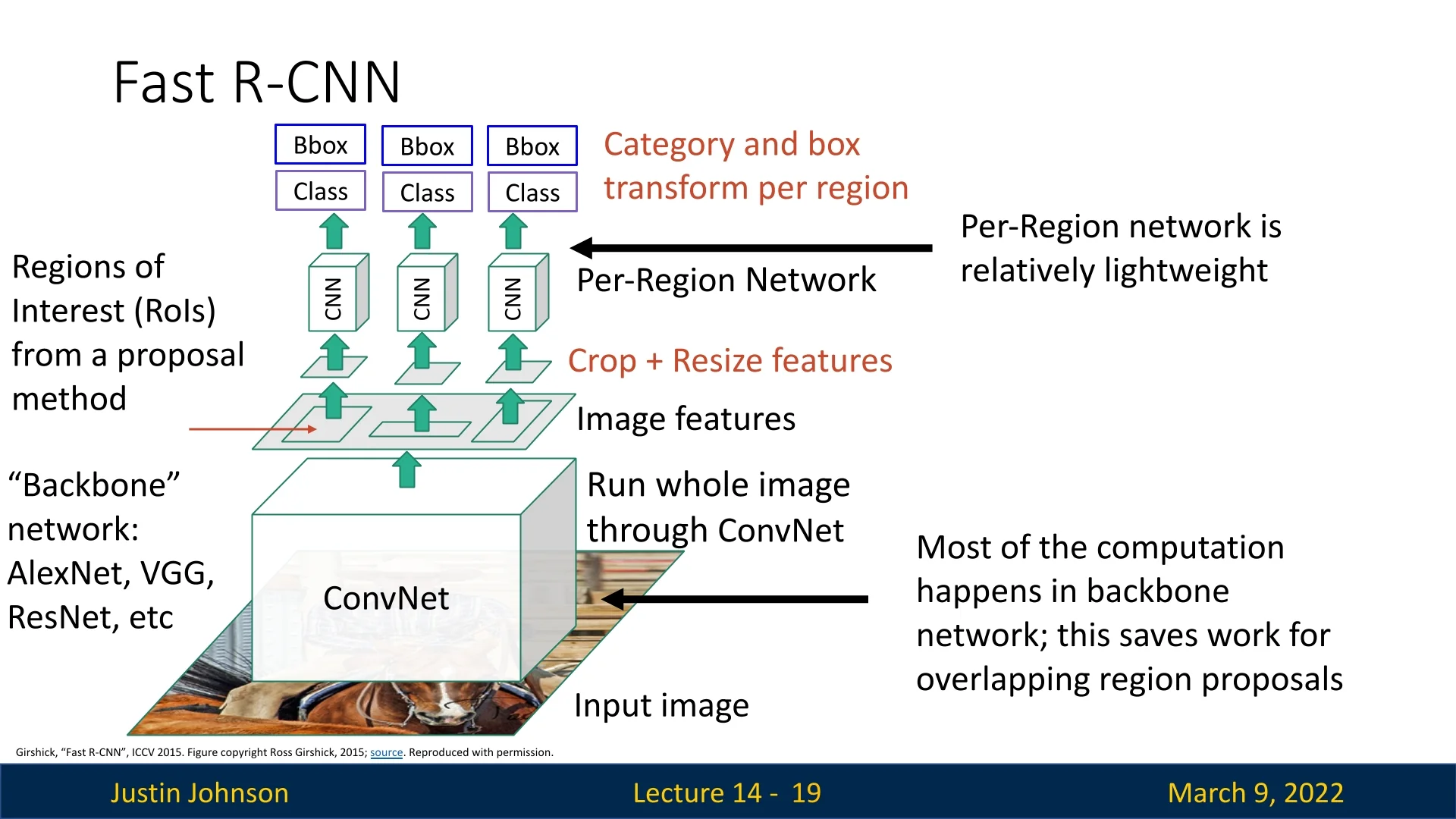
It does so by extracting a shared feature representation. Then, Region of Interest (RoI) Pooling is used to extract features corresponding to each region proposal from this shared representation. A small per-region sub-network is then applied to each extracted region to Classify the region into an object category or background, and refine the bounding box using regression.
14.2.2 Using Fully Convolutional Deep Backbones for Feature Extraction
Fast R-CNN leverages deep CNNs to extract features from the entire image in one forward pass.
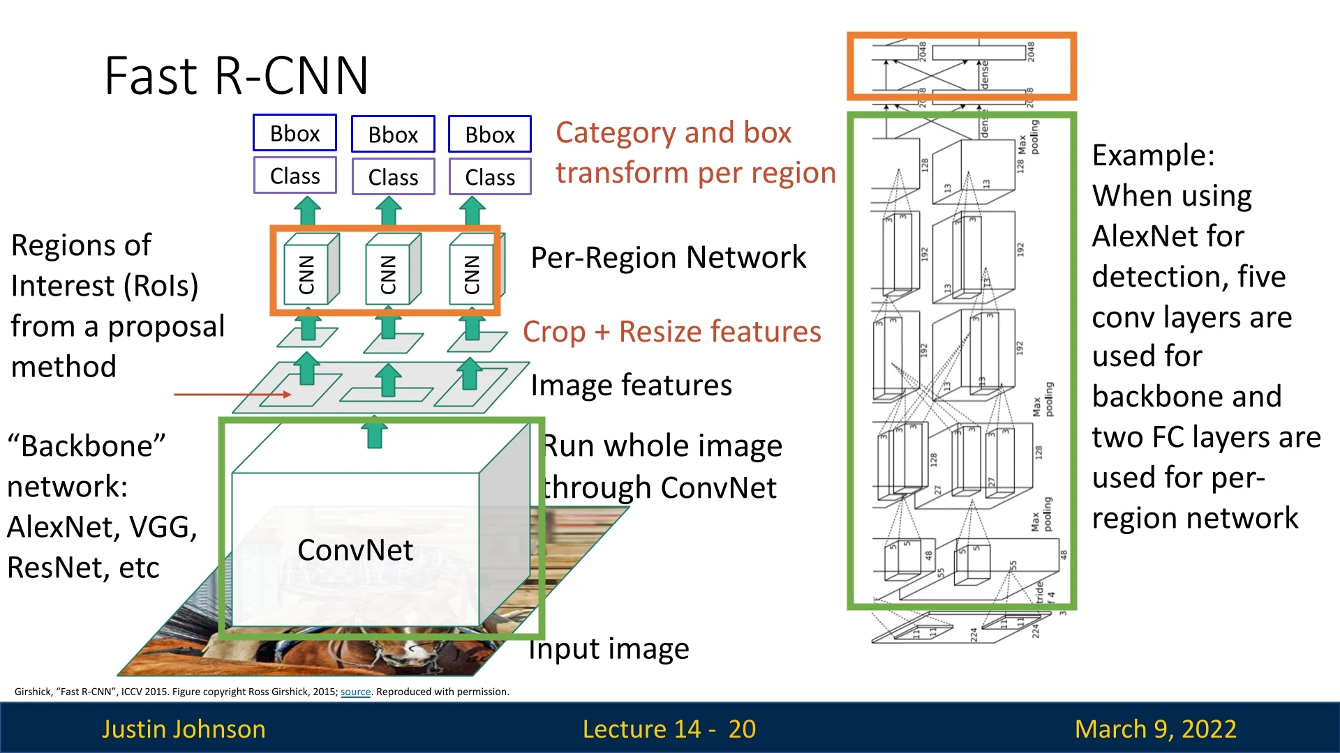
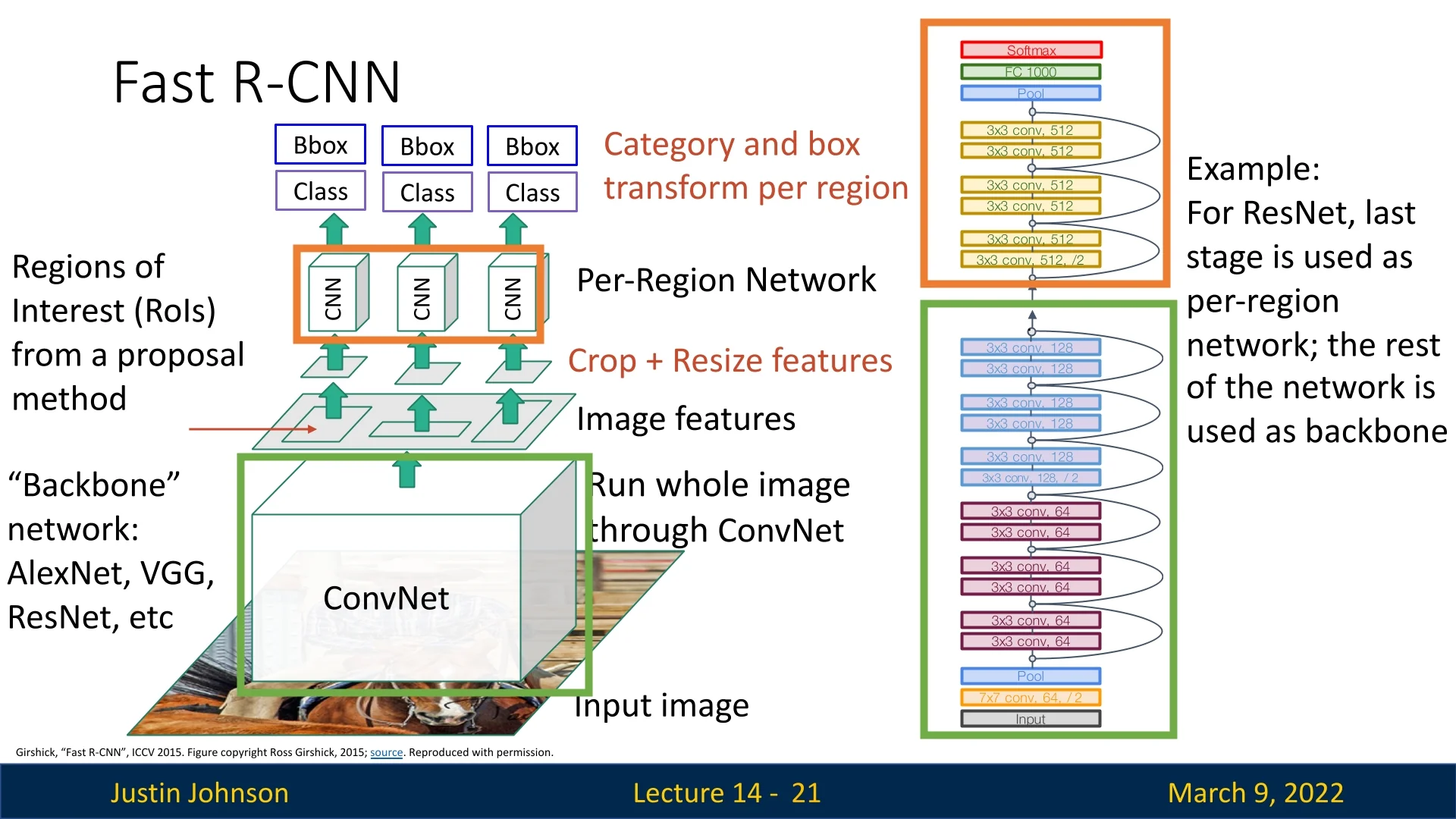
An interesting observation is that both approaches use a fully convolutional backbone.
This is deliberate, as a fully convolutional network produces a dense, spatially organized feature map in which each element corresponds directly to a specific location in the input image.
This spatial correspondence is critical for RoI pooling: it allows us to accurately map the coordinates of a region proposal (generated in the original image space) onto the feature map, so that the correct features can be “cropped out” and later pooled into a fixed-size representation.
In contrast, if the backbone ended with fully connected layers, the spatial arrangement would be lost because fully connected layers mix information from all locations. Without a maintained spatial structure, there would be no straightforward way to project a region proposal onto the feature map. Consequently, each proposal would have to be processed individually from the image itself—defeating the purpose of using a shared, efficient feature extractor.
14.2.3 Region of Interest (RoI) Pooling
In Fast R-CNN, we aim to extract feature maps corresponding to each region proposal while ensuring that the process remains differentiable so we can backpropagate gradients through the backbone CNN. This challenge is addressed using Region of Interest (RoI) Pooling.
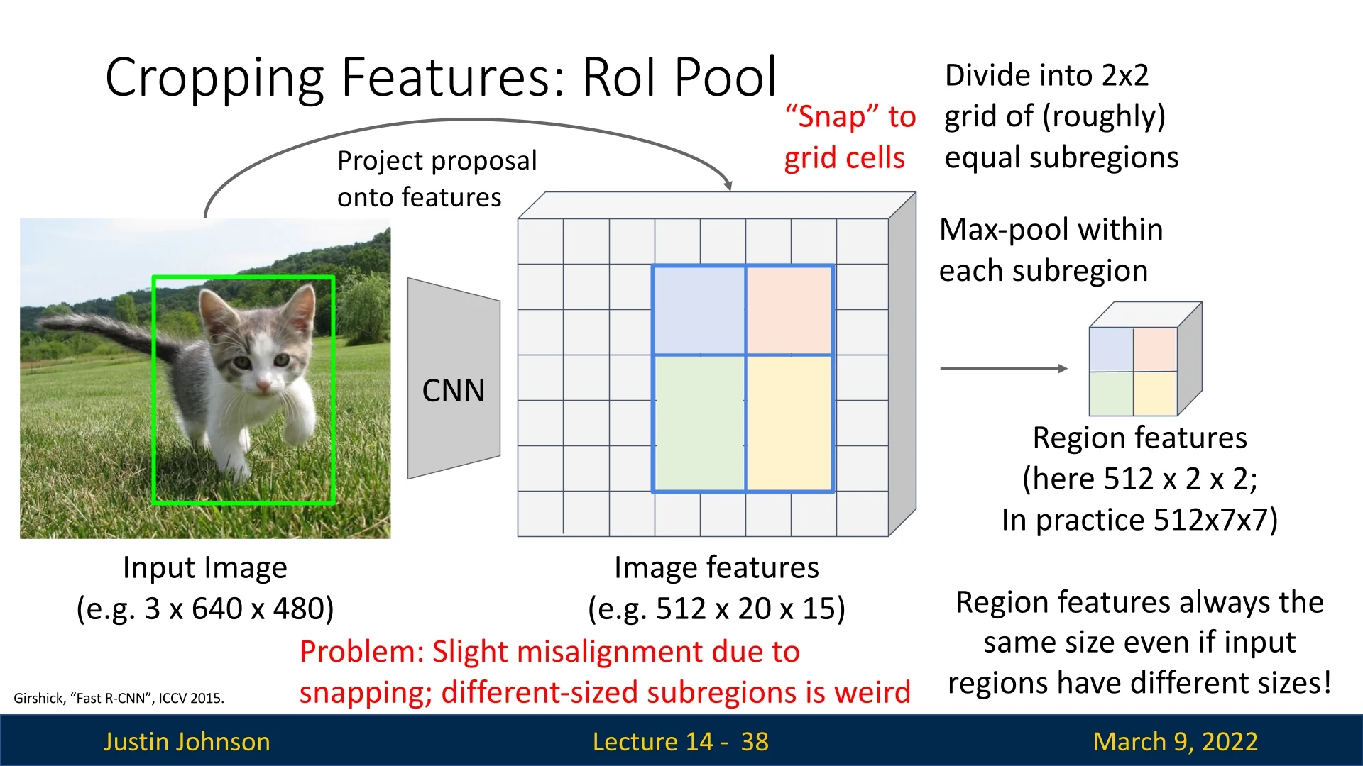
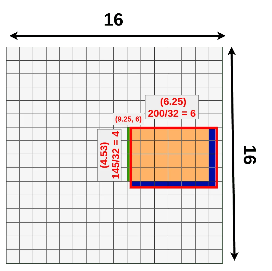
Mapping Region Proposals onto the Feature Map Region proposals—typically generated by methods such as selective search—are initially defined in the coordinate space of the original input image. However, because the backbone CNN downsamples the input by a factor \( k \) (e.g., \( k = 16 \)), these coordinates must be mapped onto the feature map. This transformation is given by:
\[ x' = \frac {x}{k}, \quad y' = \frac {y}{k}, \quad w' = \frac {w}{k}, \quad h' = \frac {h}{k} \]
where \( (x, y, w, h) \) represents the original coordinates and dimensions of the region proposal on the input image, and \( (x', y', w', h') \) represents the corresponding region on the feature map.
Since this division typically results in non-integer values (e.g., \( x' = 9.25 \)), the coordinates are quantized—usually by taking the floor function:
\[ x'' = \lfloor x' \rfloor , \quad y'' = \lfloor y' \rfloor , \quad w'' = \lfloor w' \rfloor , \quad h'' = \lfloor h' \rfloor \]
This snapping operation ensures that proposals align with the discrete grid of the feature map, making it possible to extract features corresponding to each proposal.
Dividing the Region into Fixed Bins Once the region proposal is mapped onto the feature map, the corresponding feature region is divided into a fixed number of bins. This binning ensures that all proposals—regardless of their original aspect ratio—are resized to a common spatial dimension. For example, if the target output size is \( 7 \times 7 \), the extracted region is divided into \( 7 \times 7 \) roughly equal spatial sub-regions.
Max Pooling within Each Bin For each bin, max pooling is applied across all the activations in that sub-region. This operation selects the maximum value within each bin, reducing variable-sized proposals to a uniform output shape while preserving strong feature responses. The output of RoI pooling for each proposal has a fixed spatial size, e.g., \( 7 \times 7 \times C \), where \( C \) is the number of channels in the feature map.
Summary: Key Steps in RoI Pooling
- 1.
- Scaling Region Proposals: The bounding box proposals are initially given in the coordinate space of the original image. Since the backbone CNN downsamples the input by a factor \( k \) (e.g., \( k=16 \)), the proposals must be scaled accordingly.
- 2.
- Extracting Feature Patches: The scaled bounding boxes are mapped to the corresponding feature map locations, ensuring alignment with the CNN’s output resolution.
- 3.
- Dividing into Sub-Regions: Each extracted feature patch is divided into a fixed grid of bins (e.g., \( 7 \times 7 \)), regardless of the original proposal size.
- 4.
- Max Pooling per Sub-Region: Within each bin, max pooling is applied to obtain a single representative feature value.
- 5.
- Fixed Output Size: The final output for each proposal is a tensor of shape(num_proposals, num_channels, output_size, output_size), making it suitable for downstream classification and bounding box regression.
The RoI Pooling operation can be implemented in PyTorch using a custom function that extracts fixed-size feature maps from region proposals. There is a nice implementation of [487] that follows the steps outlined earlier. If you want to understand how this method works in more detail, this is a good place to start.
Limitations of RoI Pooling A key limitation of RoI pooling is the quantization error introduced during the coordinate snapping process. Since features are assigned to discrete grid locations using floor division, minor localization errors may occur, reducing detection accuracy. This problem becomes more prominent in tasks requiring precise bounding box localization.
In addition, the fact that sub-regions are not always of the same size is also weird and may prove to be sub-optimal. Due to these problems, an improved approach called RoIAlign emerged. RoIAlign eliminates quantization errors by using bilinear interpolation instead of rounding coordinates to the nearest discrete pixel. In the next section, we will explore how RoIAlign refines feature extraction to improve object detection accuracy. Although not used in Faster R-CNN, it made its way to consequent papers like Mask R-CNN that we’ll cover later.
14.2.4 RoIAlign
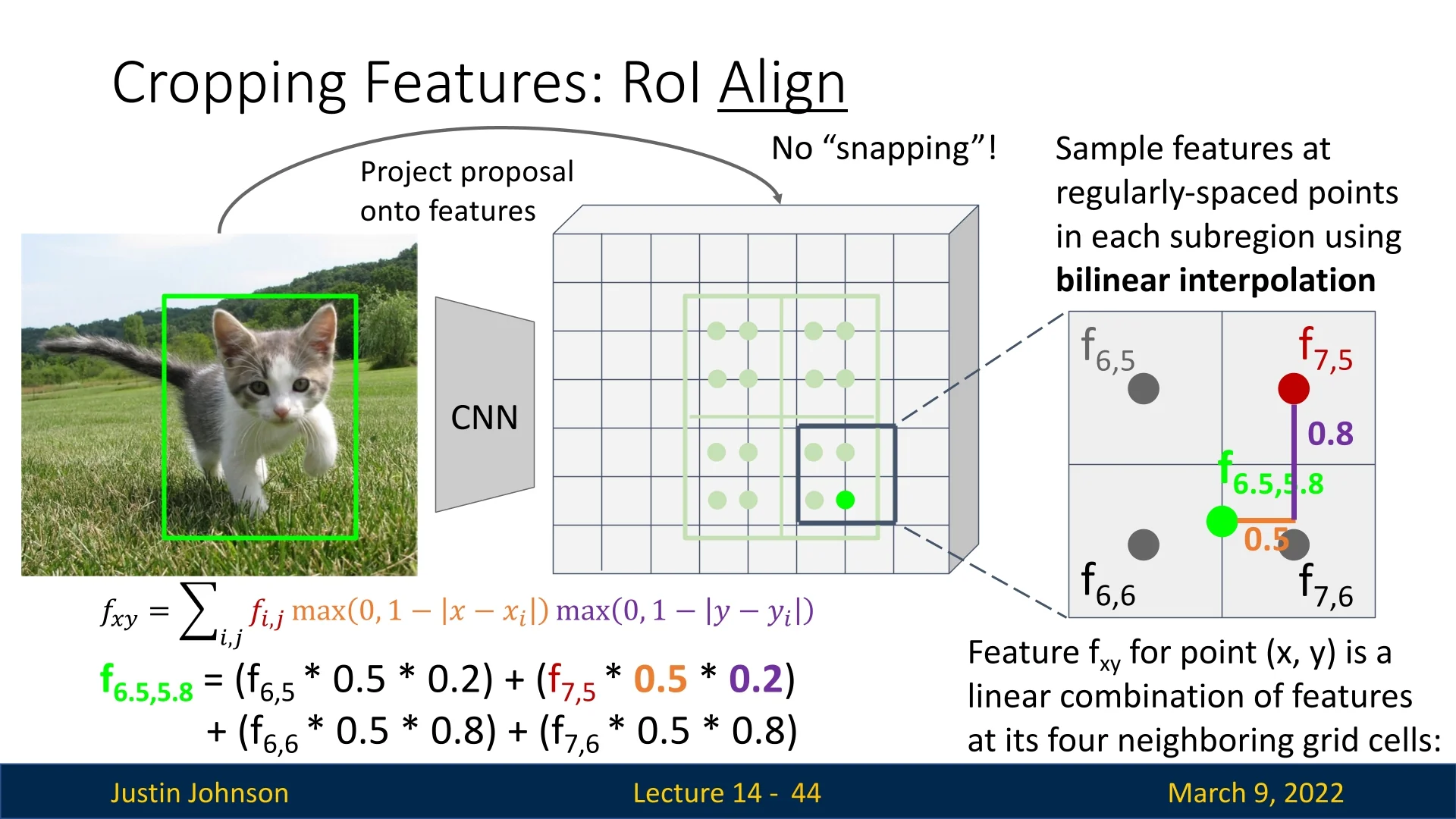
In RoIAlign we avoid any quantization (rounding) of the coordinates. Instead, we sample the feature map using bilinear interpolation to obtain sub-pixel accuracy and preserve alignment. The idea is to compute a linear combination of feature values based on their Euclidean distance to the sampling point. By doing so, each sub-region in the region of interest contributes a weighted average of the feature map’s values, thus preventing misalignments introduced by discrete rounding.
RoIAlign: A Visual Example
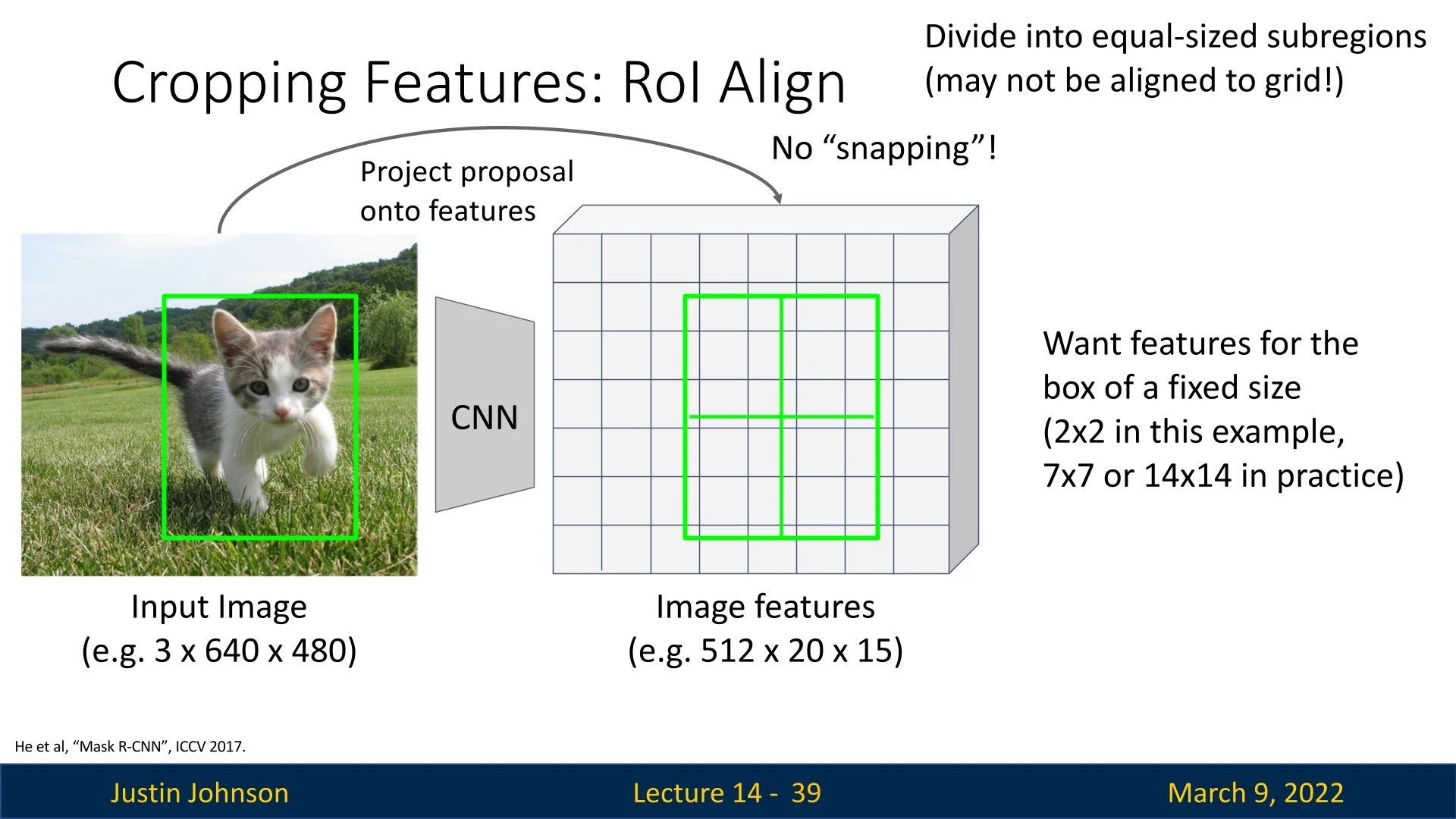
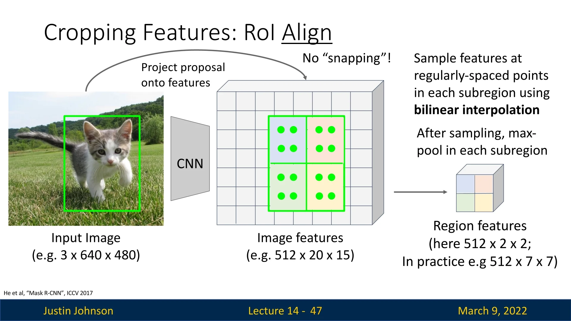
To further understand how RoIAlign works in practice, we follow a step-by-step example inspired by Justin’s lecture and [487], of which the code snippets are taken (with extra documentation I added to make it a bit more clear). This example applies RoIAlign to a region proposal of a cat image projected onto the activation/feature map. For simplicity, we use an output size of \(2 \times 2\), meaning the proposal is divided into four equal-sized sub-regions (bins), and we extract a single representative value per bin. In practice, output sizes of \(7 \times 7, 14 \times 14\) are more reasonable and common.
Step 1: Projection of Region Proposal onto the Feature Map First, we map the region proposal onto the feature map without quantization. The projected region is divided into \(2 \times 2\) bins.
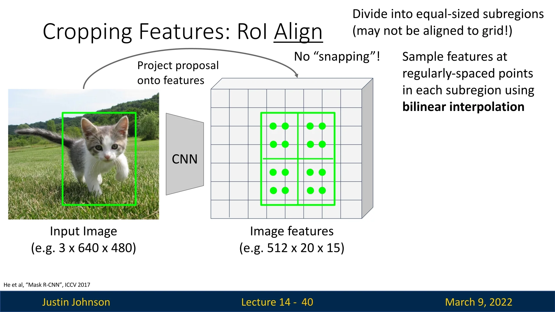
Step 2: Selecting Interpolation Points in Each Bin In RoIAlign, each bin within a region proposal is divided into regularly spaced sampling points to avoid quantization errors. Instead of snapping to the nearest discrete grid like in RoI Pooling, RoIAlign selects four interpolation points per bin to estimate the feature value using bilinear interpolation.
For each bin, four sample points are computed as follows:
- \( (x_1, y_1) \) – Top-left interpolation point
- \( (x_1, y_2) \) – Bottom-left interpolation point
- \( (x_2, y_1) \) – Top-right interpolation point
- \( (x_2, y_2) \) – Bottom-right interpolation point
As reminder, here is the part of the code in the RoIAlign method, used to compute the points to interpolate within each region of the projected proposal.
for i in range(self.output_size):
    for j in range(self.output_size):
        x_bin_strt = i * w_stride + xp0  # Bin’s top-left x coordinate
        y_bin_strt = j * h_stride + yp0  # Bin’s top-left y coordinate

        # Generate 4 points for interpolation (no rounding!)
        x1 = torch.Tensor([x_bin_strt + 0.25 * w_stride])  # Quarter into the bin
        x2 = torch.Tensor([x_bin_strt + 0.75 * w_stride])  # Three-quarters inside
        y1 = torch.Tensor([y_bin_strt + 0.25 * h_stride])  # # Quarter into the bin
        y2 = torch.Tensor([y_bin_strt + 0.75 * h_stride])  # Three-quarters inside

        # Bilinear interpolation will be performed at (x1, y1), (x1, y2), (x2,
        # y1), and (x2, y2), and these values will be used to compute the final
        # bin output for the per-region network.
For each bin (sub-region), two sample points are taken along both the \(x\)-axis and \(y\)-axis, creating a total of \(2 \times 2 = 4\) sample points. The interpolation points are systematically selected as:
\[ \{x_1, x_2\} \times \{y_1, y_2\} \]
ensuring comprehensive coverage within the bin.
Why Choose 0.25 and 0.75 for Sampling? Instead of selecting points at the exact center of each bin (\(0.5\)) or at its edges (\(0.0\) and \(1.0\)), RoIAlign samples points at \(0.25\) and \(0.75\) of the bin’s width and height. This design choice serves several purposes:
- Avoiding boundary artifacts: Sampling at \(0.0\) (bin edges) can cause rounding errors or unexpected shifts due to floating-point imprecision. Sampling at \(0.25\) and \(0.75\) keeps the points well inside the bin, ensuring they stay within the intended spatial region.
- Capturing feature variation: Sampling at just one location (e.g., the center at \(0.5\)) might miss important variations within the bin. By selecting two points per axis, we better approximate the feature distribution in that region.
- Consistent coverage: This approach systematically captures more representative “average” features, reducing the impact of noise and ensuring smooth gradient flow during backpropagation.
While RoIAlign typically uses a \(2 \times 2\) grid of sample points per bin, some implementations allow configurable sampling ratios, such as \(3 \times 3\) or higher, to improve approximation accuracy at the cost of additional computation.
By eliminating quantization artifacts and ensuring precise feature extraction, this step significantly enhances the quality of extracted region features, making RoIAlign an essential improvement over RoI Pooling.
Step 3: Mapping Sampled Points onto the Feature Grid Each of the four sampled points per bin lies within the continuous feature map, requiring us to determine its surrounding discrete grid points for bilinear interpolation. Given a sampled point \((x, y)\), it is enclosed by four neighboring integer grid points:
- \( a: (x_0, y_0) \) – Top-left corner
- \( b: (x_0, y_1) \) – Bottom-left corner
- \( c: (x_1, y_0) \) – Top-right corner
- \( d: (x_1, y_1) \) – Bottom-right corner
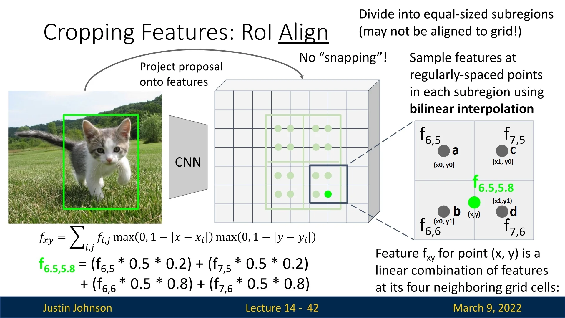
In our example, in the bottom-right bin, we consider a sampled point at \((x_2, y_2) = (6.5, 5.8)\) that is also the bottom-right point within the bin. The nearest integer grid points that enclose it are:
\[ a=(x_0 = 6, y_0 = 5), \quad b=(x_0 = 6, y_1 = 6), \quad c=(x_1 = 7, y_0 = 5), \quad d=(x_1 = 7, y_1 = 6). \]
These four points are used for interpolation, ensuring that each sampled feature value is derived from its surrounding grid points rather than being snapped to the nearest one.
To determine these enclosing grid points programmatically, we perform the following computations:
# Find the integer corners surrounding (x, y)
x0 = torch.floor(x).type(torch.cuda.LongTensor)
x1 = x0 + 1
y0 = torch.floor(y).type(torch.cuda.LongTensor)
y1 = y0 + 1

# Clamp these coordinates to the image boundary to avoid out-of-range indexing
x0 = torch.clamp(x0, 0, img.shape[1] - 1)
x1 = torch.clamp(x1, 0, img.shape[1] - 1)
y0 = torch.clamp(y0, 0, img.shape[0] - 1)
y1 = torch.clamp(y1, 0, img.shape[0] - 1)

# Extract feature values at the four surrounding grid points
Ia = img[y0, x0]  # Top-left corner
Ib = img[y1, x0]  # Bottom-left corner
Ic = img[y0, x1]  # Top-right corner
Id = img[y1, x1]  # Bottom-right corner
These four feature values \((I_a, I_b, I_c, I_d)\) serve as the basis for bilinear interpolation. Instead of directly snapping \((x, y)\) to the nearest feature grid location, we compute a weighted average of these values, using their relative distances as interpolation weights.
By mapping sampled points onto discrete grid locations in this manner, RoIAlign ensures that every proposal maintains precise alignment with the backbone’s feature map, preserving sub-pixel accuracy and avoiding misalignment errors caused by quantization.
Step 4: Computing Bilinear Interpolation Weights Once the four nearest integer grid points for a sampled point \((x,y)\) have been identified, we compute weights that determine each corner’s contribution to the interpolated value. These weights are based on the relative distances between \((x,y)\) and the four grid points.
Normalization Constant and Its Interpretation The normalization constant is given by \[ \mbox{norm_const} = \frac {1}{(x_1 - x_0)(y_1 - y_0)}, \] which is the inverse of the area of the rectangle formed by the grid points \((x_0,y_0)\), \((x_1,y_0)\), \((x_0,y_1)\), and \((x_1,y_1)\). In many cases, including our example, this rectangle is a unit square (i.e., \(x_1 - x_0 = 1\) and \(y_1 - y_0 = 1\)), so the normalization constant is 1. This constant ensures that the computed weights form a convex combination that sums to 1.
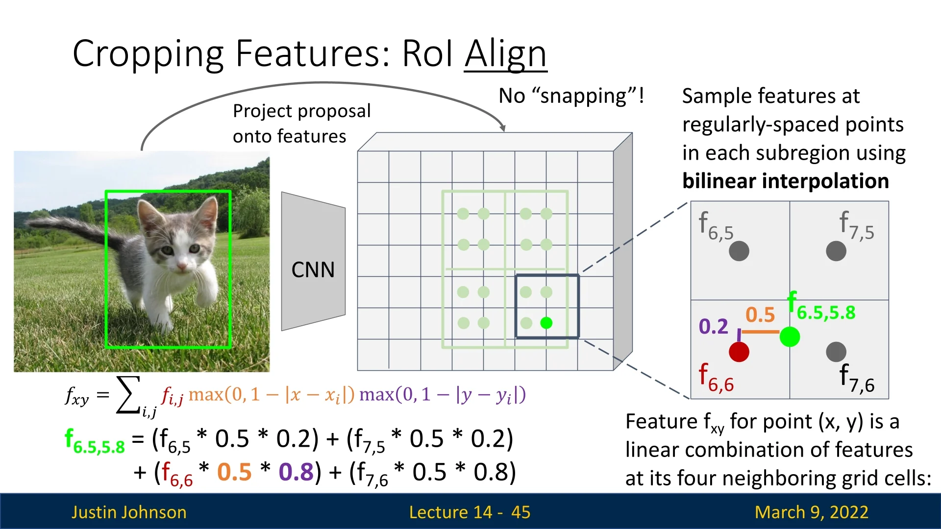
Weight Computation for Each Corner For a sampled point \((x,y) = (6.5, 5.8)\), assume the four surrounding grid points are: \[ (x_0,y_0) = (6,5), \quad (x_1,y_0) = (7,5), \quad (x_0,y_1) = (6,6), \quad (x_1,y_1) = (7,6). \] We compute the distances: \[ x_1 - x = 7 - 6.5 = 0.5, \quad x - x_0 = 6.5 - 6 = 0.5, \] \[ y_1 - y = 6 - 5.8 = 0.2, \quad y - y_0 = 5.8 - 5 = 0.8. \] The weight for each grid point is the product of the fractional distances along the x and y axes, meaning, each weight is determined by how far the sampled point is from a particular corner, considering both x and y distances. The horizontal and vertical contributions are combined as: - \((x_1 - x) / (x_1 - x_0)\) → Fraction of the width from \((x, y)\) to the right boundary. - \((x - x_0) / (x_1 - x_0)\) → Fraction from \((x, y)\) to the left boundary. - \((y_1 - y) / (y_1 - y_0)\) → Fraction of the height from \((x, y)\) to the bottom boundary. - \((y - y_0) / (y_1 - y_0)\) → Fraction from \((x, y)\) to the top boundary.
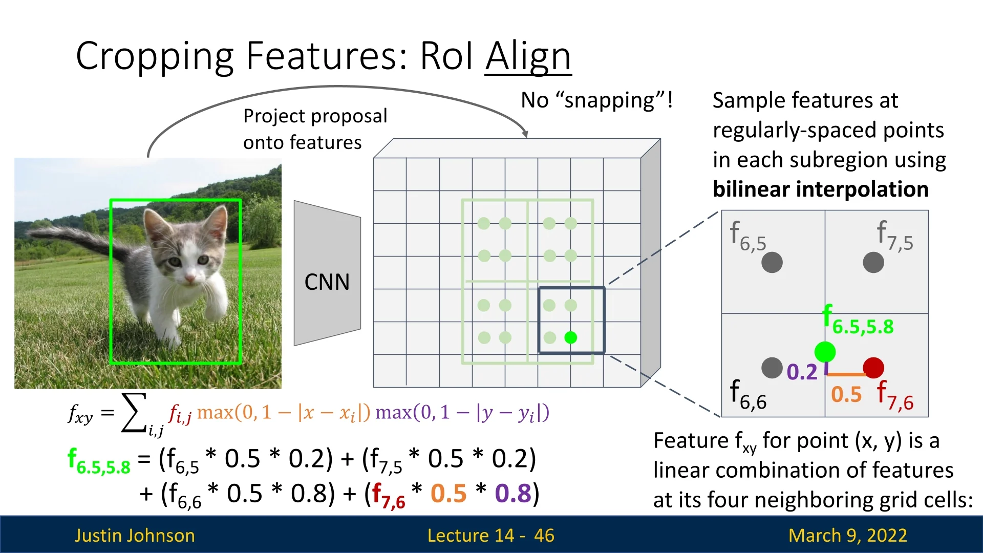
Therefore, for the top-left corner (denoted \(w_a\)), the weight is given by: \[ w_a = (x_1 - x) \cdot (y_1 - y) = 0.5 \times 0.2 = 0.1. \] Similarly, for the top-right corner (denoted \(w_c\)): \[ w_c = (x - x_0) \cdot (y_1 - y) = 0.5 \times 0.2 = 0.1. \] For the bottom-left corner (denoted \(w_b\)): \[ w_b = (x_1 - x) \cdot (y - y_0) = 0.5 \times 0.8 = 0.4, \] and for the bottom-right corner (denoted \(w_d\)): \[ w_d = (x - x_0) \cdot (y - y_0) = 0.5 \times 0.8 = 0.4. \] Thus, the weights satisfy \[ w_a + w_b + w_c + w_d = 0.1 + 0.4 + 0.1 + 0.4 = 1.0. \]

Step 5: Computing the Interpolated Feature Value Once the interpolation weights have been determined, we compute the interpolated feature value at \((x, y)\) as a weighted sum of the four surrounding feature grid values:
\[ f_{xy} = w_a f_{x_0 y_0} + w_b f_{x_0 y_1} + w_c f_{x_1 y_0} + w_d f_{x_1 y_1} \]
Each weight determines the contribution of the corresponding grid point to the interpolated value. Since closer grid points have higher weights, they exert more influence over the final value than those further away.
Example Computation For the sampled point \((x,y) = (6.5, 5.8)\), using previously computed weights: \[ w_a = 0.1, \quad w_b = 0.4, \quad w_c = 0.1, \quad w_d = 0.4 \]
and the corresponding feature values from the activation map:
\[ I_a = f_{6,5}, \quad I_b = f_{6,6}, \quad I_c = f_{7,5}, \quad I_d = f_{7,6} \]
we compute the interpolated feature value as:
\[ f_{6.5,5.8} = (0.1 \times f_{6,5}) + (0.4 \times f_{6,6}) + (0.1 \times f_{7,5}) + (0.4 \times f_{7,6}) \]
Step 6: Aggregating Interpolated Values After computing the interpolated feature values for all sampled points, we aggregate them using either:
- Average pooling: The final value is the mean of all interpolated feature values.
- Max pooling: The final value is the maximum of all interpolated values.
In Justin’s example, max pooling is used: \[ \mbox{bin value} = \max (v_1, v_2, v_3, v_4) \]
Final Output After iterating over all bins, the final RoI feature map is constructed, with each bin containing an aggregated value from bilinear interpolation. The per-proposal network then uses this structured feature representation for classification and bounding-box regression.
- RoIAlign eliminates the quantization error of RoI Pooling by leveraging bilinear interpolation.
- The interpolation process ensures precise feature extraction, leading to improved localization accuracy.
- The final feature map maintains a fixed size per RoI, making it compatible with subsequent per-region classifiers and regressors.
Hence, RoIAlign is a core component of modern architectures used for detection and segmentation like Mask R-CNN.
RoIAlign Important Implementation Parts in PyTorch Following the implementation of [487], here are the important code snippets that illustrate how RoIAlign works, helping to see how the process looks like from start to finish.
def _roi_align(self, features, scaled_proposal):
    """Given feature layers and scaled proposals return bilinear interpolated
    points in feature layer

    Args:
    features (torch.Tensor): Tensor of shape <channels x height x width>
    scaled_proposal (list of torch.Tensor): Each tensor is a bbox by which we
    will extract features from features Tensor
    """

    _, num_channels, h, w = features.shape

    # (xp0, yp0) = top-left corner of projected proposal, (xp1, yp1) = bottom-right corner.
    xp0, yp0, xp1, yp1 = scaled_proposal
    p_width = xp1 - xp0
    p_height = yp1 - yp0

    ’’’
    If we want to output a nxn tensor to the per-proposal network, then output_size = n.
    The number of sub-regions we’ll produce, like in RoIPool, will be nxn as well.
    The height and width of each sub-region will be equal, as the regions are now of exactly the same size,
    but crucially we no longer snap to integer boundaries.
    Each sub-region’s representative value will be a linear combination of the pixel values
    that this sub-region covers(via bilinear interpolation).
    ’’’
    w_stride = p_width / self.output_size  # The width of each sub-region
    h_stride = p_height / self.output_size  # The height of each sub-region

    interp_features = torch.zeros((num_channels, self.output_size, self.output_size))

    for i in range(self.output_size):
        for j in range(self.output_size):
            # top-left x coordinate of the i-th sub-region
            x_bin_strt = i * w_stride + xp0
            # top-left y coordinate of the j-th sub-region
            y_bin_strt = j * h_stride + yp0

            # generate 4 points for interpolation (no rounding!)
            x1 = torch.Tensor([x_bin_strt + 0.25*w_stride])  # quarter in the bin (x-axis)
            x2 = torch.Tensor([x_bin_strt + 0.75*w_stride])  # three-quarters in the bin (x-axis)
            y1 = torch.Tensor([y_bin_strt + 0.25*h_stride])  # quarter in the bin (y-axis)
            y2 = torch.Tensor([y_bin_strt + 0.75*h_stride])  # three-quarters in the bin (y-axis)

            ’’’
            We sample 2 points along x(0.25 and 0.75 of the bin width)
            and 2 points along y(0.25 and 0.75 of the bin height).
            This yields 2 x 2 = 4 sample points per bin.

            Why at 0.25 and 0.75?
            1) Avoid boundaries: Sampling at 0 or 1 might cause rounding/boundary issues.
                2) Capture variation: Multiple sample points per bin help represent
            the internal structure better than a single center point.
                3) Consistent coverage: 0.25 and 0.75 systematically offer an even "spread"
            in each dimension, approximating the average effectively.
                ’’’

            for c in range(num_channels):
                # features[0, c] is the single-channel feature map for channel c
                img = features[0, c]
                v1 = bilinear_interpolate(img, x1, y1)
                v2 = bilinear_interpolate(img, x1, y2)
                v3 = bilinear_interpolate(img, x2, y1)
                v4 = bilinear_interpolate(img, x2, y2)

                ’’’
                v1, v2, v3, v4 are the bilinear-interpolated values at the four sample points.
                We average these 4 values to get a single value for bin(i, j) and channel c.
                Note: In some cases, one might take max instead of average
                (mimicking max pooling). This is what Justin shows in the lecture. Hence, he takes max(v1, v2, v3, v4) instead.
                ’’’
                interp_features[c, j, i] = (v1 + v2 + v3 + v4) / 4

                return interp_features
We now understand the RoIAlign high-level flow. Next, let us examine how bilinear interpolation works for the four regularly sampled points inside each bin, of which we’ll compute the output bin value for the per-proposal network later.
def bilinear_interpolate(img, x, y):
    ’’’ We are given a point(x, y) that might not be a pixel coordinate,
    and we want to interpolate its feature value from the surrounding pixels.
    ’’’

    # find the integer corners that surround (x, y)
    x0 = torch.floor(x).type(torch.cuda.LongTensor)
    x1 = x0 + 1
    y0 = torch.floor(y).type(torch.cuda.LongTensor)
    y1 = y0 + 1

    # clamp these coordinates to the image boundary to avoid indexing out of range
    x0 = torch.clamp(x0, 0, img.shape[1] - 1)
    x1 = torch.clamp(x1, 0, img.shape[1] - 1)
    y0 = torch.clamp(y0, 0, img.shape[0] - 1)
    y1 = torch.clamp(y1, 0, img.shape[0] - 1)

    # top-left, bottom-left, top-right, bottom-right corner values
    Ia = img[y0, x0]
    Ib = img[y1, x0]
    Ic = img[y0, x1]
    Id = img[y1, x1]

    ’’’
    Next, we compute the weights for each corner. The idea:
    - (x1 - x) -> how far we are from the right edge in the x direction
    - (x - x0) -> how far we are from the left edge in the x direction
    - (y1 - y) -> how far we are from the bottom edge in the y direction
    - (y - y0) -> how far we are from the top edge in the y direction

    We multiply these "partial distances" and then normalize by the total "area"
    ((x1 - x0)*(y1 - y0)) so that wa+wb+wc+wd = 1.
    ’’’

    norm_const = 1 / ((x1.type(torch.float32) - x0.type(torch.float32)) *
    (y1.type(torch.float32) - y0.type(torch.float32)))

    wa = (x1.type(torch.float32) - x) * (y1.type(torch.float32) - y) * norm_const
    wb = (x1.type(torch.float32) - x) * (y - y0.type(torch.float32)) * norm_const
    wc = (x - x0.type(torch.float32)) * (y1.type(torch.float32) - y) * norm_const
    wd = (x - x0.type(torch.float32)) * (y - y0.type(torch.float32)) * norm_const

    # final bilinear interpolation: weighted sum of the four corners
    return torch.t(torch.t(Ia) * wa) + torch.t(torch.t(Ib) * wb) + \
    torch.t(torch.t(Ic) * wc) + torch.t(torch.t(Id) * wd)
14.3 Faster R-CNN: Faster Proposals Using RPNs
14.3.1 Fast R-CNN Bottleneck: Region Proposal Computation
Although Fast R-CNN optimized the detection pipeline, the slowest component remained the region proposal generation. The external algorithm used, such as Selective Search, was still running on the CPU, making it a major bottleneck.
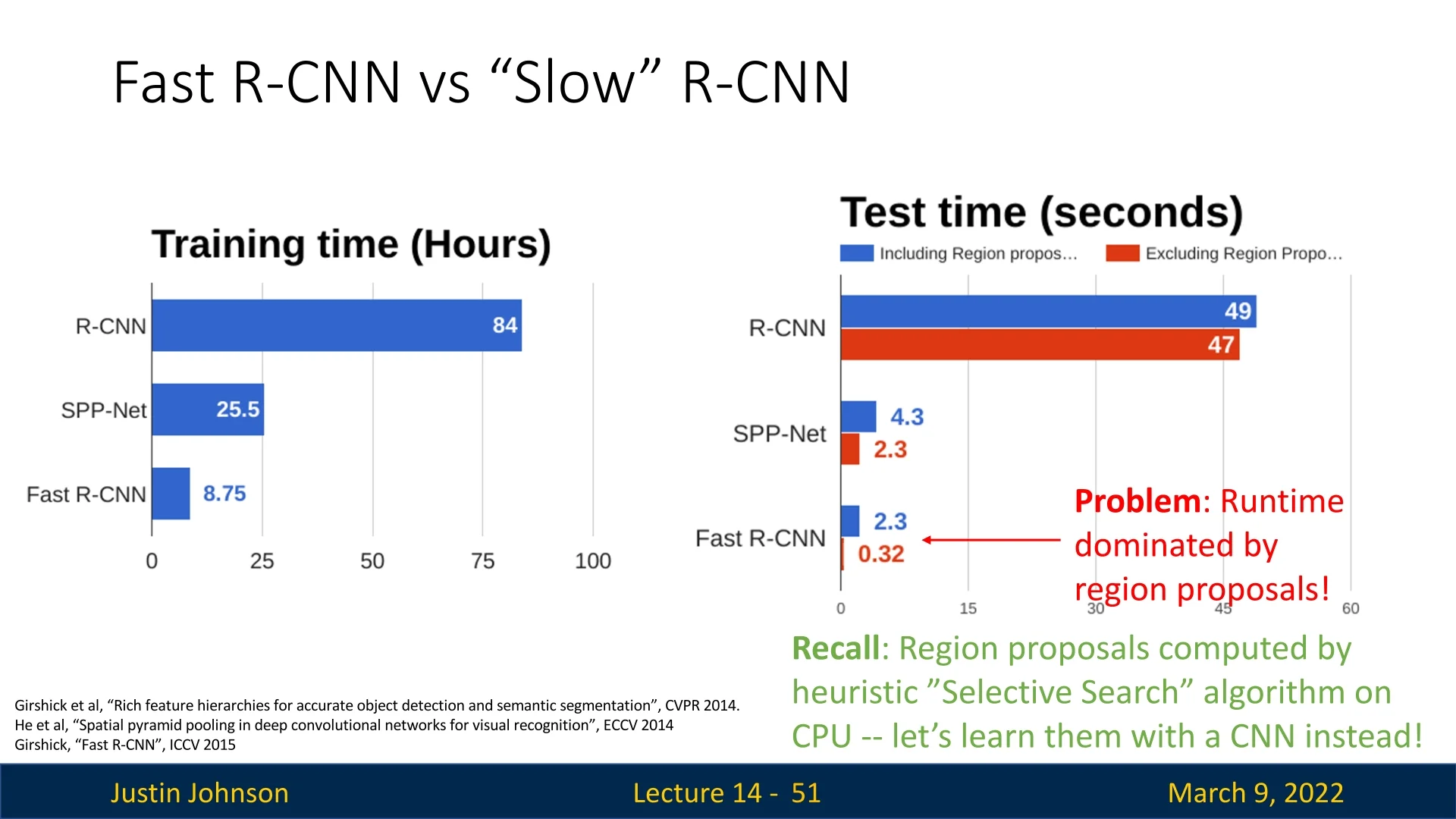
As shown in Figure 14.14, even though feature extraction and classification were now efficient, generating proposals using heuristic-based methods still consumed a significant portion of the runtime.
14.3.2 Towards Faster Region Proposals: Learning Proposals with CNNs
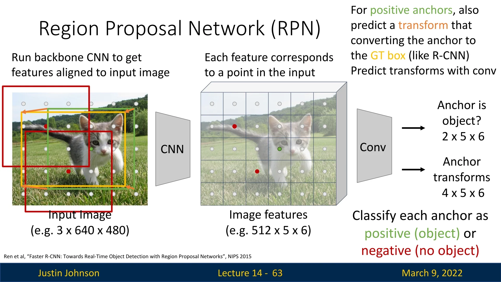
The natural next step in improving object detection efficiency was to replace the handcrafted, CPU-based proposal generation process with a learnable, CNN-based alternative. Faster R-CNN introduced the Region Proposal Network (RPN) [539], an architecture that predicts object proposals directly from the feature maps produced by the backbone CNN. This approach integrates proposal generation into the deep learning pipeline, eliminating the need for slow external algorithms.
The key idea behind RPNs is:
- Use convolutional feature maps to directly predict high-quality object proposals.
- Train the proposal generator jointly with the rest of the detection pipeline.
- Make the entire object detection process fully differentiable and GPU-accelerated.
By replacing Selective Search with an RPN, Faster R-CNN eliminates the last major bottleneck in Fast R-CNN and makes object detection significantly faster while maintaining high accuracy. In the next section, we will explore the details of Region Proposal Networks and their role in Faster R-CNN.
14.3.3 Region Proposal Networks (RPNs)
How RPNs Work Instead of using a separate region proposal algorithm, RPNs generate proposals directly from the shared feature map produced by a deep CNN backbone. The process follows these steps:
- 1.
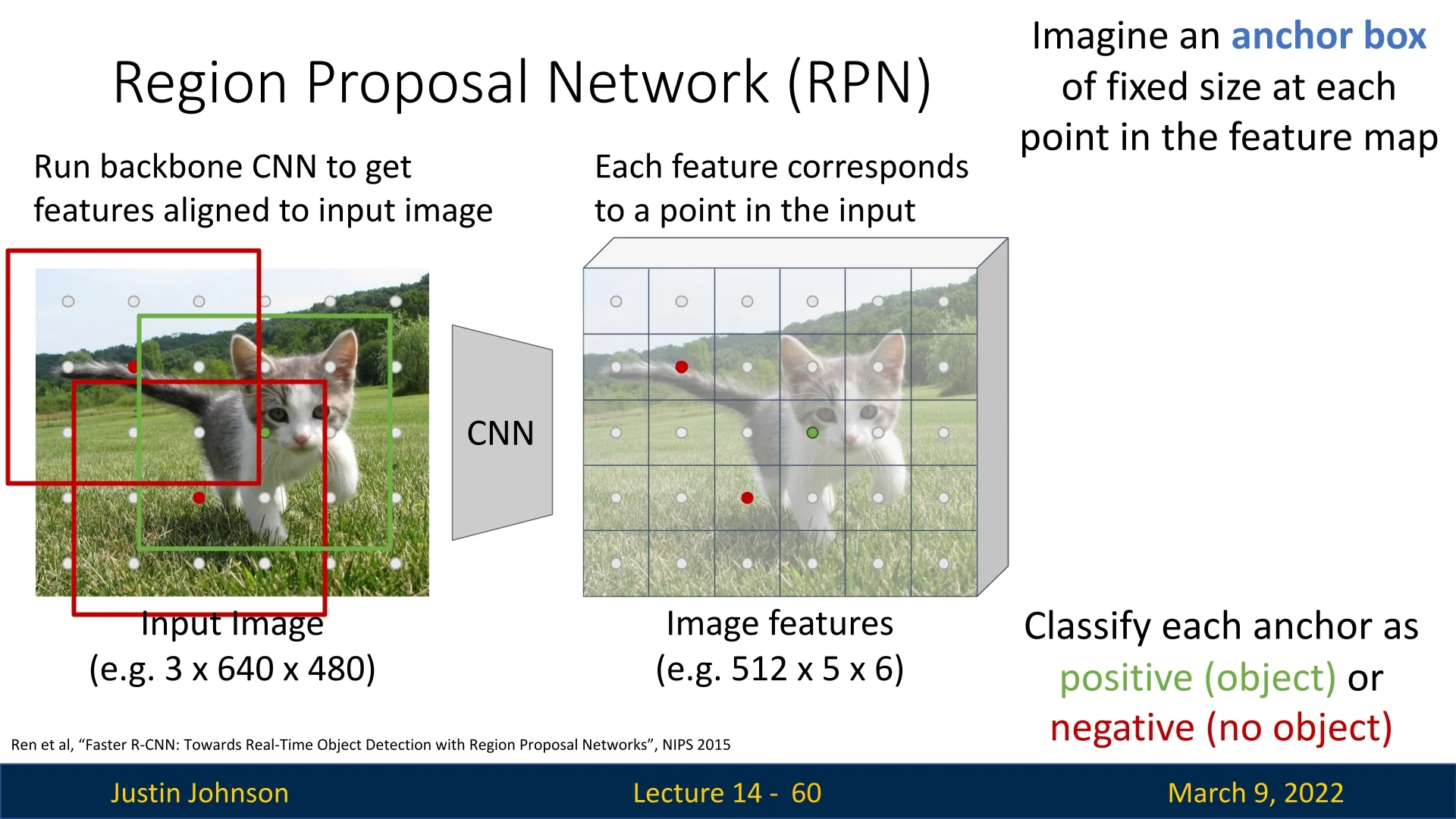
- Feature Extraction: The backbone CNN extracts a feature map from the input image while preserving spatial alignment.
- 2.
- Anchor Generation: At each spatial location on the feature map, predefined anchor boxes (of multiple sizes and aspect ratios) serve as candidate proposals.
- 3.
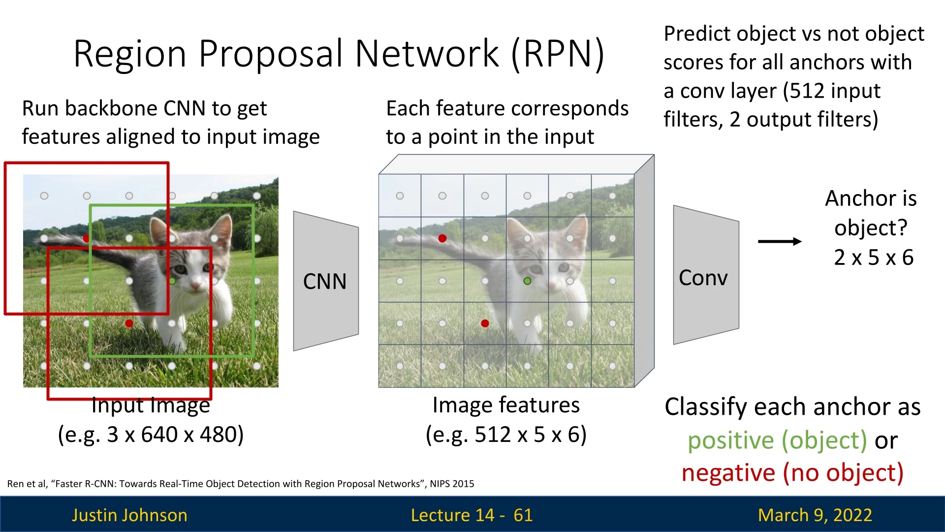
- Objectness Classification: A small convolutional layer predicts whether each anchor contains an object.
- 4.
- Bounding Box Regression: For positive anchors, another convolutional layer predicts the transformation required to refine the anchor into a better-fitting bounding box.
Since the RPN operates directly on the shared feature map, it adds minimal computational cost—it is simply a small set of convolutional layers applied to the extracted backbone features. This allows the model to generate high-quality proposals without needing separate, slow region proposal methods.
Anchor Boxes: Handling Scale and Aspect Ratio Variations In object detection, objects appear in diverse shapes and sizes. A single fixed-size proposal per spatial location would fail to capture this variability. To address this, RPNs generate proposals using a set of predefined anchor boxes at each spatial location on the feature map. Each anchor serves as a reference box that can be classified and refined to better fit actual objects.
At each spatial location, RPNs generate \(K\) anchors with:
- Different scales – Capturing small, medium, and large objects.
- Different aspect ratios – Adapting to tall, square, and wide objects.
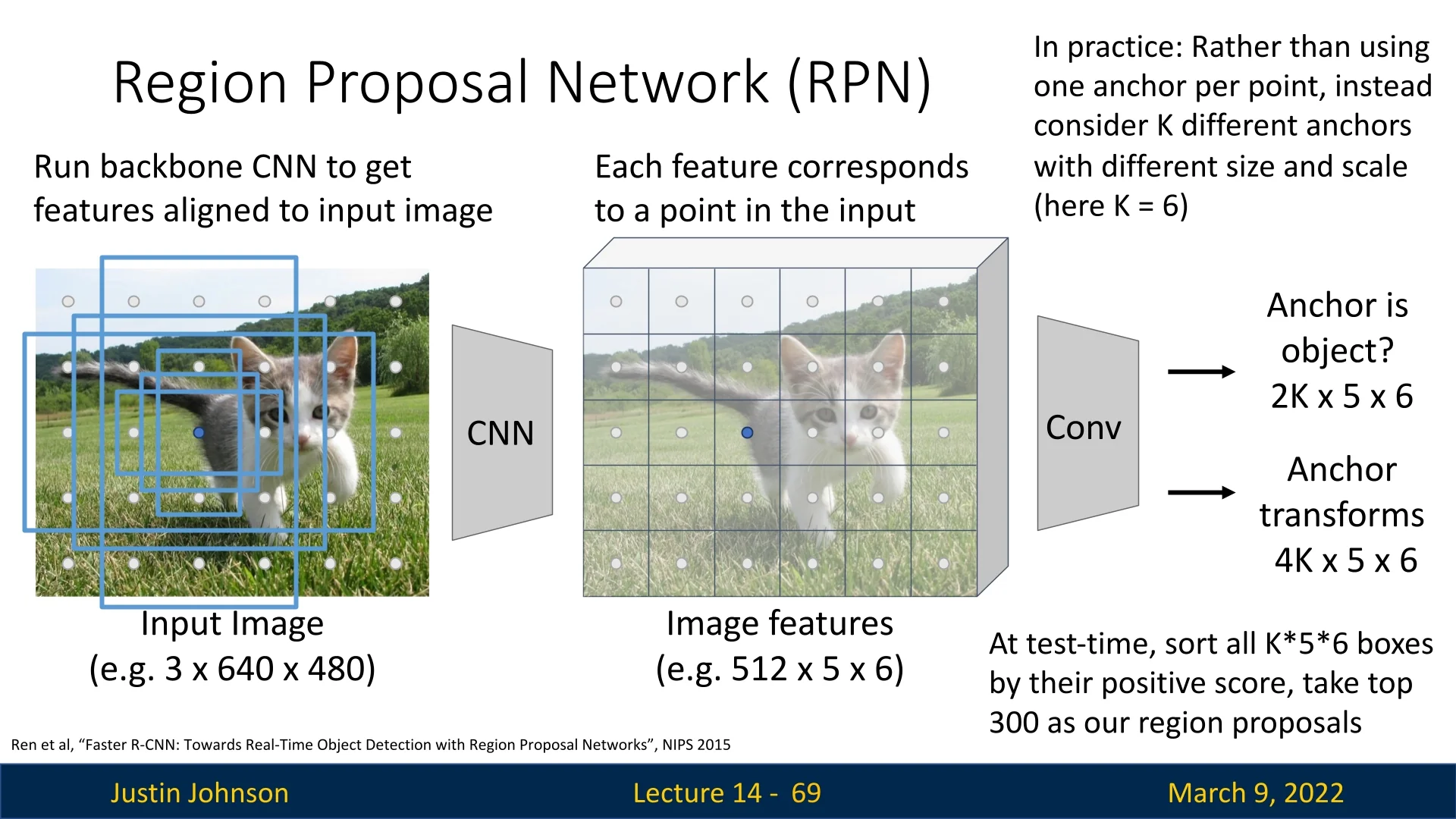
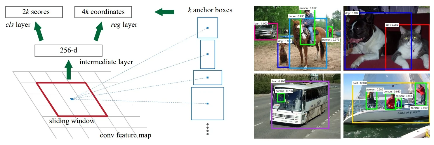
The original Faster R-CNN paper used 9 anchors per location (3 scales \(\times \) 3 aspect ratios). For each anchor, the RPN predicts:
- Objectness Score – A binary classification indicating whether the anchor contains a foreground object or belongs to background. Conceptually, this is just logistic regression: for each anchor we want a probability \(p(\mbox{object} \mid \mbox{anchor})\). In practice, most implementations parameterize this as two logits per anchor (foreground and background) and apply a softmax followed by a cross-entropy loss. For the binary case, this two-logit softmax formulation is mathematically equivalent to a single-logit sigmoid (standard logistic regression); it is simply more convenient to implement and extend to multi-class settings.
- Bounding Box Transform – A transformation \((t_x, t_y, t_w, t_h)\) refining the anchor box.
These predictions are made using a small CNN applied to the feature map. The classification branch outputs a \(2K\)-channel score map (for \(K\) anchors per location), i.e., for each spatial location it predicts two logits (foreground / background) for each of the \(K\) anchors. If the RPN feature map has spatial size \(5 \times 6\), this corresponds to a tensor of shape \(2K \times 5 \times 6\) per training image. The regression branch outputs a \(4K\)-channel transform map per spatial location, yielding an output tensor of shape \(4K \times 5 \times 6\) per training image.
Bounding Box Refinement: Aligning Anchors to Objects Even with multiple anchors per location, an anchor may not perfectly match an object’s true dimensions. To improve localization, the RPN predicts a refinement transformation, similar to what R-CNN and Fast R-CNN do for final detections. For details on bounding box transformations, refer to Section §14.
The refinement transformation is parameterized as follows:
\[ t_x = \frac {b_x - p_x}{p_w}, \quad t_y = \frac {b_y - p_y}{p_h}, \quad t_w = \ln \left ( \frac {b_w}{p_w} \right ), \quad t_h = \ln \left ( \frac {b_h}{p_h} \right ) \]
where \((p_x, p_y, p_w, p_h)\) are the anchor box parameters and \((b_x, b_y, b_w, b_h)\) are the refined bounding box parameters.
Unlike traditional proposal generation methods, RPNs train the proposal generation process jointly with the feature extraction backbone, allowing the network to learn proposals that are well-suited for the final detection task. This integration improves both accuracy and computational efficiency.
Training RPNs: Assigning Labels to Anchors To train a Region Proposal Network (RPN), we must assign labels to the anchor boxes, distinguishing between positive, negative, and neutral examples. This labeling process is crucial for optimizing both classification (objectness score) and bounding box regression.
- Positive anchors: Anchors that have an IoU \(\geq 0.7\) with at least one ground-truth box are considered positive.
- Negative anchors: Anchors with IoU \(< 0.3\) with all ground-truth boxes are labeled negative.
- Neutral anchors: Anchors with an IoU between 0.3 and 0.7 are ignored during training.
Since anchor boxes serve as a reference for object detection, positive anchors are used to compute both classification and regression losses.
Negative anchors, on the other hand, only contribute to the classification loss, ensuring the RPN learns to distinguish objects from background effectively.
Loss Function for RPN Training The RPN is trained using a multi-task loss function that jointly optimizes object classification and bounding box regression:
\[ L(\{p_i\}, \{t_i\}) = \frac {1}{N_{\mbox{cls}}} \sum _{i} L_{\mbox{cls}}(p_i, p^*_i) + \lambda \frac {1}{N_{\mbox{reg}}} \sum _{i} p^*_i L_{\mbox{reg}}(t_i, t^*_i) \]
where:
- \( p_i \) is the predicted probability of anchor \( i \) containing an object.
- \( p^*_i \) is the ground-truth label (1 for objects, 0 for background).
- \( t_i \) is the predicted bounding box transform for anchor \( i \).
- \( t^*_i \) is the ground-truth bounding box transform.
- \( L_{\mbox{cls}} \) is the binary cross-entropy loss for object classification.
- \( L_{\mbox{reg}} \) is the smooth \( L_1 \) loss applied only to positive anchors.
- \( N_{\mbox{cls}} \) and \( N_{\mbox{reg}} \) are normalization terms.
- \( \lambda \) is a balancing factor, typically set to 10.
This loss function ensures that classification and bounding box regression are optimized simultaneously.
Assigning Ground-Truth Bounding Boxes to Anchors Each positive anchor is assigned to the ground-truth box that has the maximum IoU with it. This ensures that the best-matching ground-truth object supervises the training of the anchor’s bounding box regression.
- If an anchor has \(\mbox{IoU} \geq 0.7\) with multiple ground-truth boxes, it is assigned to the object with which it has the highest IoU.
- Each ground-truth box must be matched to at least one anchor. If no anchor has \(\mbox{IoU} \geq 0.7\) with a given ground-truth box, the anchor with the highest IoU is forcibly assigned to it.
This matching process ensures that all ground-truth objects are covered by at least one anchor, enabling the RPN to propose accurate regions for all objects in an image.
Smooth \( L_1 \) Loss for Bounding Box Regression To refine anchor boxes into accurate region proposals, Faster R-CNN employs the smooth \( L_1 \) loss, which is defined as:
\[ L_{\mbox{reg}}(t_i, t^*_i) = \begin {cases} 0.5 (t_i - t^*_i)^2, & \mbox{if } |t_i - t^*_i| < 1 \\ |t_i - t^*_i| - 0.5, & \mbox{otherwise} \end {cases} \]
This loss behaves like an \( L_2 \) loss (squared error) when the error is small, ensuring smooth gradients for small offsets. However, for larger errors, it switches to an \( L_1 \) loss (absolute error), preventing large outliers from dominating the training process.
Why Smooth \( L_1 \) Instead of \( L_2 \) Loss?
- Robustness to Outliers: Unlike the \( L_2 \) loss, which heavily penalizes large errors, the smooth \( L_1 \) loss reduces the influence of extreme outliers.
- Stable Training: The transition from quadratic to linear loss ensures that large localization errors do not cause excessively high gradients, making optimization more stable.
- Better Localization: Since bounding box predictions can have large variations, the smooth \( L_1 \) loss allows more effective training, focusing on improving the fine alignment of predicted boxes.
By integrating the smooth \( L_1 \) loss into the RPN’s training objective, Faster R-CNN achieves more accurate and stable region proposals, leading to improved object detection performance.
Why Use Negative Anchors? Negative anchors (IoU \(<\) 0.3) play a crucial role in training the RPN. Without them, the model would lack supervision on how to classify background regions, leading to an excess of false positives. Negative anchors:
- Ensure the RPN learns to reject background regions by reinforcing the binary classification task.
- Provide a balance between object detection and background rejection, making the system more robust (ensuring that the RPN does not overfit to detecting only foreground objects).
Enrichment 14.3.3.1: Training Region Proposal Networks (RPNs)
The Region Proposal Network (RPN) [538] is a learnable module for generating class-agnostic object proposals from convolutional feature maps. Below is a complete walkthrough of the training process.
1. Input Feature Map Given an input image \( I \in \mathbb {R}^{H \times W \times 3} \), a CNN backbone (e.g., VGG-16, ResNet-50) produces a feature map of spatial dimensions: \[ F \in \mathbb {R}^{H' \times W' \times C'}, \quad \mbox{where } H' = H/s,\, W' = W/s. \] The stride \( s \) reflects total downsampling (often \( s = 16 \)).
A shared \(3 \times 3\) conv is applied across all spatial locations to extract intermediate features:
# Shared intermediate 3x3 conv
rpn_conv = nn.Conv2d(C_prime, 512, kernel_size=3, padding=1)
inter_features = F.relu(rpn_conv(featmap))  # (B, 512, H’, W’)
Each spatial location corresponds to a position in the original image and will be associated with \(K\) anchor boxes.
3. RPN Heads: Anchor-wise Classification and Regression Two parallel \(1\times 1\) conv layers produce:
- Objectness scores: \(2K\) channels (foreground vs. background for each anchor),
- BBox deltas: \(4K\) channels (\(\Delta x, \Delta y, \Delta w, \Delta h\) for each anchor).
rpn_cls_logits = nn.Conv2d(512, 2 * K, kernel_size=1)(inter_features)
rpn_bbox_deltas = nn.Conv2d(512, 4 * K, kernel_size=1)(inter_features)
These outputs are reshaped to \((B, H' \times W' \times K, 2)\) and \((B, H' \times W' \times K, 4)\) respectively during training for loss computation, to associate each anchor with its corresponding predictions:
rpn_cls_logits = rpn_cls_logits.permute(0, 2, 3, 1).reshape(B, -1, 2)
rpn_bbox_deltas = rpn_bbox_deltas.permute(0, 2, 3, 1).reshape(B, -1, 4)
4. Anchor Labeling and Ground Truth Assignment To train the network, we must determine which anchors are positive (object), negative (background), or ignored. For this, we compute the IoU (Intersection-over-Union) between each anchor and each ground-truth box:
- Positive: An anchor is labeled positive if it has an IoU \(\ge 0.7\) with any GT box, or if it is the highest-IoU anchor for a given GT.
- Negative: Labeled background if it has IoU \(\le 0.3\) with all GT boxes.
- Ignored: Anchors with intermediate IoU scores are not used in the loss.
labels, matched_gt_boxes = assign_labels(all_anchors, gt_boxes)
# labels: 1 = positive, 0 = negative, -1 = ignore
pos_inds = torch.where(labels == 1)[0]  # Indices of positive anchors
fg_bg_inds = torch.where(labels != -1)[0]  # Anchors involved in loss
5. Bounding-Box Regression Targets For each positive anchor, we compute the offset required to transform the anchor into its assigned ground-truth box. These offsets form the regression targets.
Each target is parameterized as: \[ \Delta x = \frac {x_{\mbox{gt}} - x_{\mbox{anchor}}}{w_{\mbox{anchor}}}, \quad \Delta y = \frac {y_{\mbox{gt}} - y_{\mbox{anchor}}}{h_{\mbox{anchor}}}, \quad \Delta w = \log \frac {w_{\mbox{gt}}}{w_{\mbox{anchor}}}, \quad \Delta h = \log \frac {h_{\mbox{gt}}}{h_{\mbox{anchor}}}. \]
These values measure:
- The relative translation (\(\Delta x, \Delta y\)) of the ground-truth box center w.r.t. the anchor box.
- The log-scale change (\(\Delta w, \Delta h\)) needed to stretch the anchor’s width/height to match the ground truth.
bbox_targets = compute_regression_targets(anchors[pos_inds], matched_gt_boxes[pos_inds])
# Shape: (N_pos, 4)
These targets serve as supervision: the network learns to predict these deltas for each positive anchor.
6. Loss Computation The RPN is trained using a multi-task loss: \[ \mathcal {L}_{\mbox{RPN}} = \frac {1}{N_{\mbox{cls}}} \sum _i \mathcal {L}_{\mbox{cls}}(p_i, p_i^*) + \lambda \cdot \frac {1}{N_{\mbox{reg}}} \sum _i \mathbb {1}_{\{p_i^* = 1\}} \cdot \mathcal {L}_{\mbox{reg}}(t_i, t_i^*), \] where:
- \(p_i\): predicted objectness logits (before softmax),
- \(p_i^*\): binary GT label (1 for object, 0 for background),
- \(t_i\): predicted regression deltas (rpn_bbox_deltas),
- \(t_i^*\): GT regression target (bbox_targets).
cls_loss = F.cross_entropy(rpn_cls_logits[fg_bg_inds], labels[fg_bg_inds])
reg_loss = smooth_l1_loss(rpn_bbox_deltas[pos_inds], bbox_targets)
total_loss = cls_loss + lambda_ * reg_loss
Note: During training, we do not decode or apply the predicted deltas to anchors. Instead, we supervise the raw predicted deltas directly, using regression targets computed from fixed anchor–GT box pairs. This ensures stable optimization, as the anchors remain fixed while the network learns to output precise \((\Delta x, \Delta y, \Delta w, \Delta h)\) shifts. Only at inference time do we apply these predicted offsets to anchors to produce proposal boxes.
Inference: Generating Region Proposals At inference time, the RPN processes all anchor boxes across the image and filters out low-confidence proposals to retain the most relevant ones. The process consists of the following steps:
- 1.
- Compute objectness scores: The classification branch predicts an object score for each anchor box.
- 2.
- Sort proposals by objectness score: The top-scoring anchors are retained for further processing.
- 3.
- Apply Non-Maximum Suppression (NMS): Overlapping proposals with a high IoU are removed, keeping only the most confident detections.
- 4.
- Select the top \(N\) proposals (e.g., 300 proposals) as final region proposals for Fast R-CNN.
By filtering out redundant and low-confidence proposals, this step improves both efficiency and accuracy, ensuring that only the most relevant regions are processed by the detector.
RPNs Improve Region Proposal Generation Compared to previous region proposal methods like Selective Search, RPNs introduce several key advantages:
- Speed: RPNs operate directly on the backbone’s shared feature map as a small conv head. Proposal generation becomes a single GPU pass instead of a slow, separate CPU algorithm.
- Learned “Objectness”: Because the RPN is trained jointly with the detector, it learns which regions in feature space are likely to contain any object, rather than relying on hand-crafted low-level grouping cues. This produces proposals that are more relevant to the downstream detection task (fewer obvious background regions, more boxes covering real objects).
- More Precise Localization: Each positive anchor is not only classified as “object vs. background,” but also refined by a learned bounding box regressor that predicts offsets \(((t_x, t_y, t_w, t_h))\). This allows the network to adjust coarse anchors to tightly hug the true object boundaries, resulting in proposals that overlap ground-truth boxes much more accurately than the fixed, heuristic boxes from Selective Search.
Thus, Faster R-CNN achieves real-time object detection by integrating RPNs and Fast R-CNN into a unified pipeline.
14.3.4 Faster R-CNN Loss in Practice: Joint Training with Four Losses
Joint Training in Faster R-CNN Unlike previous object detection pipelines where region proposal generation and object classification were trained separately, Faster R-CNN jointly trains both the RPN and the object detector. This results in a fully end-to-end learnable system with a four-part loss function:
\[ L = L_{\mbox{cls}}^{\mbox{RPN}} + L_{\mbox{reg}}^{\mbox{RPN}} + L_{\mbox{cls}}^{\mbox{Fast R-CNN}} + L_{\mbox{reg}}^{\mbox{Fast R-CNN}} \]
- \( L_{\mbox{cls}}^{\mbox{RPN}} \) – Classifies anchor boxes as object vs. background.
- \( L_{\mbox{reg}}^{\mbox{RPN}} \) – Refines anchor boxes to generate high-quality proposals.
- \( L_{\mbox{cls}}^{\mbox{Fast R-CNN}} \) – Classifies refined proposals into object categories.
- \( L_{\mbox{reg}}^{\mbox{Fast R-CNN}} \) – Further refines bounding box localization.
By training the RPN together with the detection network, the region proposal generation and object detection become more aligned, improving both efficiency and accuracy.
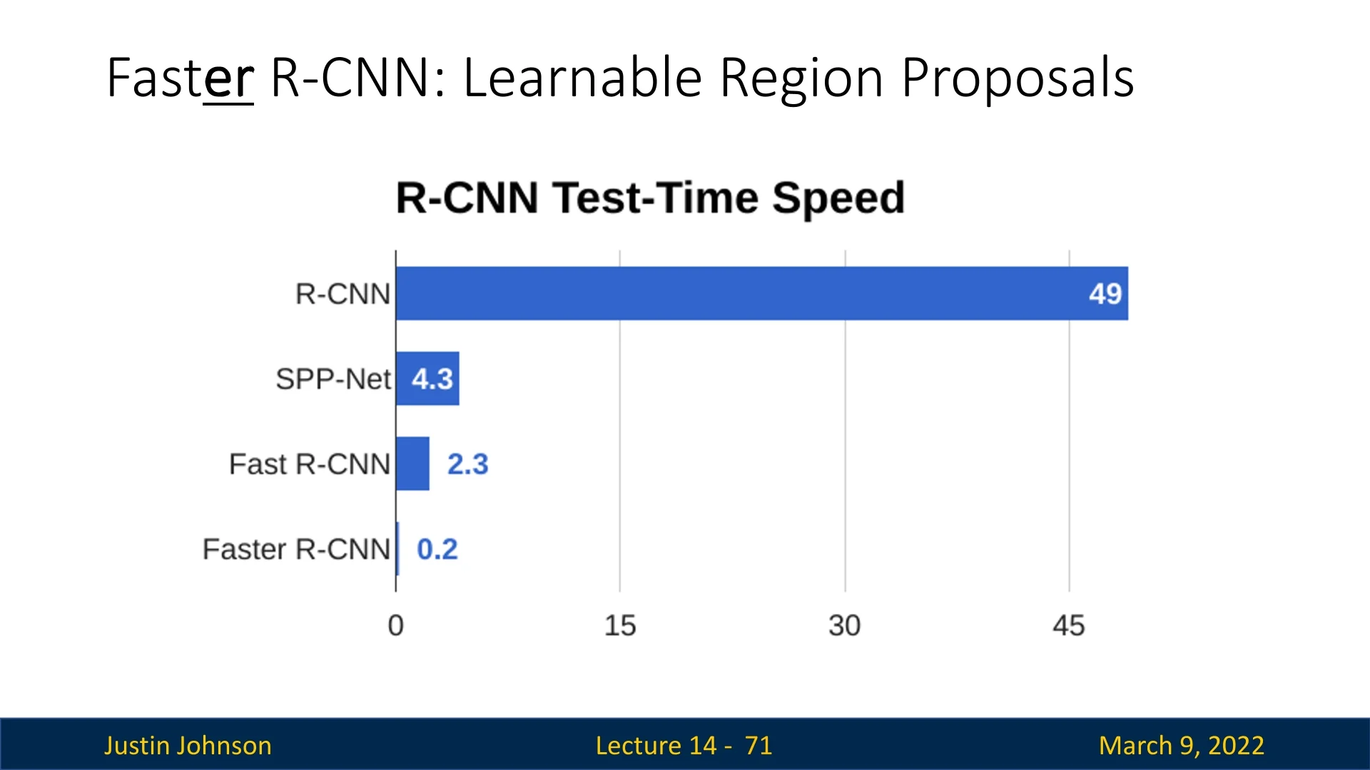
How RPN Improves Inference Speed Before Faster R-CNN, Fast R-CNN significantly reduced inference time compared to R-CNN by sharing computations. However, it still relied on external region proposal methods such as Selective Search, which were computationally expensive. Faster R-CNN eliminates this bottleneck by using RPN to generate region proposals directly from the feature map.
Key Takeaways:
- Eliminating external region proposals – Instead of using a separate CPU-based region proposal method (e.g., Selective Search), Faster R-CNN predicts region proposals using CNNs.
- Fully convolutional region proposals – The RPN operates as a small, efficient convolutional network on top of the shared feature map.
- Dramatic speedup – With RPN, the overall test-time speed improves from 2.3s in Fast R-CNN to just 0.2s in Faster R-CNN, making real-time object detection more feasible.
By integrating joint training, region proposal learning, and feature sharing, Faster R-CNN achieves significant improvements over previous detectors, making it one of the most influential object detection models.
14.3.5 Feature Pyramid Networks (FPNs): Multi-Scale Feature Learning
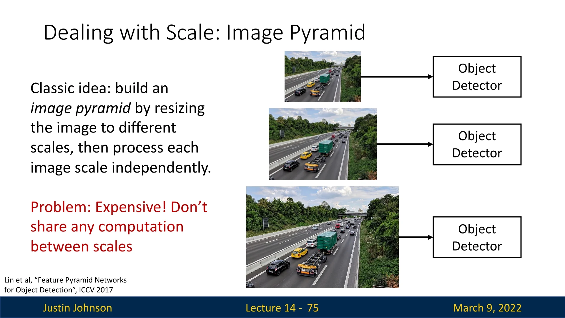
Detecting objects of varying scales is a fundamental challenge in object detection. Traditional methods attempted to improve scale invariance by constructing an image pyramid, where the image is resized to multiple scales and processed separately by the detector. This approach is computationally expensive since the network must process the same image multiple times.
Feature Pyramid Networks: A More Efficient Approach
Rather than resizing the image, Lin et al. (2017) [367] proposed leveraging the inherent hierarchical structure of convolutional neural networks (CNNs). Since CNNs naturally extract features at multiple resolutions due to their deep architecture, FPNs attach independent detectors to features from multiple levels of the backbone. This enables the model to handle objects at different scales without requiring multiple forward passes.
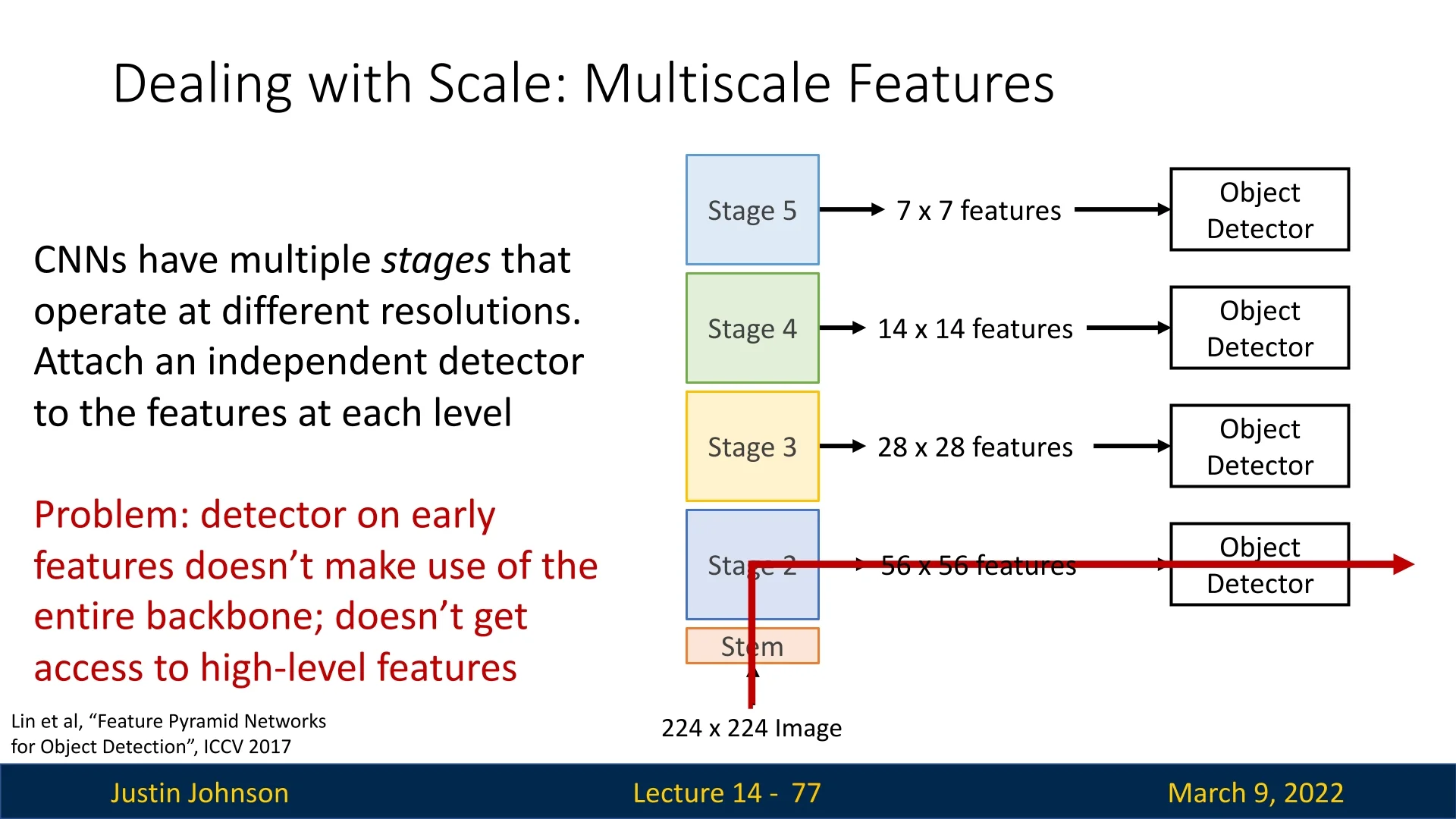
Enhancing Low-Level Features with High-Level Semantics
A major drawback of using early-stage CNN features for object detection is that they lack semantic richness. Lower layers in CNNs retain high spatial resolution but primarily capture edges and textures, whereas deeper layers encode more complex features but at a lower resolution. This results in a trade-off: high-resolution features lack meaningful context, while low-resolution features are more informative but spatially coarse.
To address this, FPNs introduce top-down connections that propagate high-level information back to lower-resolution feature maps.
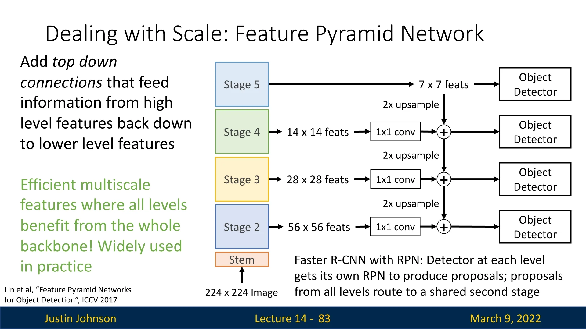
Specifically, the process consists of the following steps:
- 1.
- Each feature map from the backbone undergoes a \(1\times 1\) convolution to change its channel dimensionality. This ensures that features from different levels are compatible when combined.
- 2.
- The highest-level feature map (smallest spatial size, richest semantic information) is directly used as the starting point for the top-down pathway.
- 3.
- The lower-resolution feature maps are then progressively upsampled using bilinear interpolation or transposed convolution (also known as deconvolution) to match the spatial resolution of the next finer feature map.
- 4.
- The upsampled feature map is then element-wise added to the corresponding feature map from the backbone (which retains high spatial resolution but lacks deep semantic information).
- 5.
- Finally, the fused feature maps are further processed by a \(3\times 3\) convolution to smooth out artifacts introduced by upsampling and fusion before being used for object detection.
How Upsampling Works in FPNs Upsampling is a crucial operation in FPNs since it allows coarse but high-level features to be brought into alignment with finer-resolution feature maps. This is typically done in one of two ways:
- Bilinear Interpolation: A non-learnable method we’ve covered that interpolates pixel values based on surrounding features, and can be used to produce smooth upscaled feature maps.
- Transposed Convolution (Deconvolution): A learnable operation that applies upsampling with trainable filters, allowing the network to learn an optimal way to refine features during backpropagation. We’ll cover it in more detail later, when we’ll discuss segmentation.
By applying these top-down connections, FPNs create a hierarchical feature representation where all levels of the feature pyramid benefit from deep semantic information. This significantly improves object detection performance, especially for small objects, by ensuring that all feature levels contribute meaningful information to the final detections.
Combining Results from Multiple Feature Levels
Once object detections are generated from multiple feature levels, they must be merged to produce a final prediction. The standard approach is to apply Non-Maximum Suppression (NMS) across all detections:
- Sort all detected bounding boxes by confidence score.
- Iteratively suppress overlapping boxes with lower confidence, ensuring that redundant detections do not appear in the final output.
Advantages of FPNs Feature Pyramid Networks offer several key advantages over traditional multi-scale detection approaches:
- Efficient multi-scale feature extraction – The network processes the image only once, rather than at multiple scales.
- Enhanced small-object detection – Lower-resolution feature maps retain fine details while incorporating high-level semantics.
- Lightweight and scalable – The additional computational cost of FPNs is minimal compared to constructing an image pyramid.
By efficiently integrating information from different levels of a CNN, FPNs have become a standard component in modern object detection architectures, including Faster R-CNN.
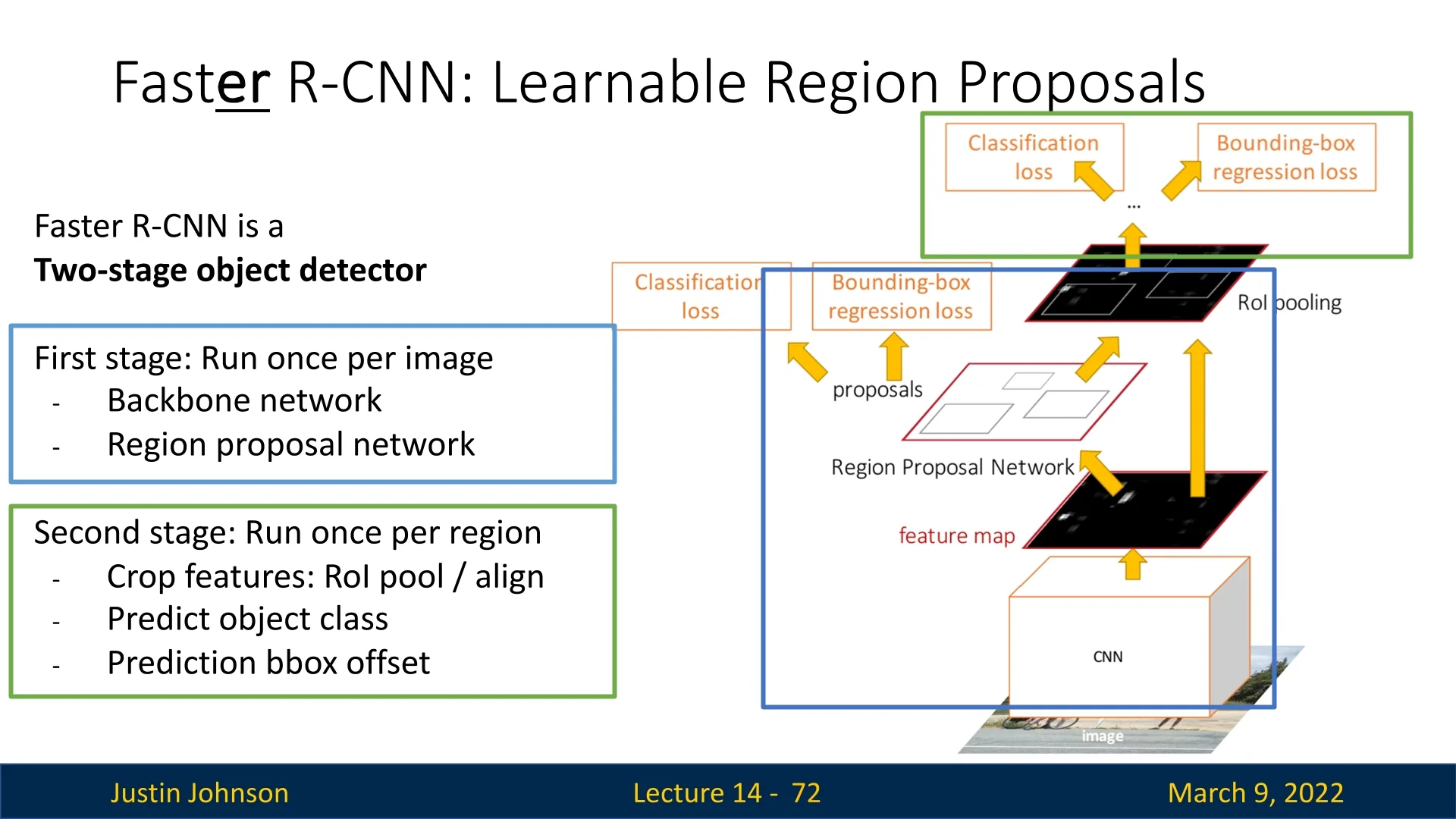
The Two-Stage Object Detection Pipeline Faster R-CNN is a two-stage object detector, meaning the detection process is divided into two sequential steps:
- 1.
- Stage 1: Region Proposal Generation
- The backbone CNN processes the entire image once to generate a feature map.
- The Region Proposal Network (RPN) applies convolutional layers to the feature map and outputs a set of region proposals, each with an objectness score and bounding box transform.
- The top \(N\) proposals (e.g., 300) are selected using Non-Maximum Suppression (NMS) to remove redundant boxes.
- 2.
- Stage 2: Object Detection and Classification
- The extracted feature map is cropped using RoIPooling, producing fixed-size feature vectors for each proposal.
- Each proposal is classified into an object category or background.
- A final bounding box refinement transformation improves localization accuracy.
This two-stage approach provides high accuracy but comes at the cost of increased computational complexity. Faster R-CNN significantly improves inference speed over its predecessors, yet the sequential pipeline—first generate proposals, then run a per-proposal classifier and regressor—still limits real-time performance.
A natural follow-up question is: do we really need a separate second stage at all? Notice that the RPN in Stage 1 is already a small, fully convolutional network that scans the feature map and predicts both an objectness score and bounding box offsets for many locations. In other words, it is almost a detector by itself—just with a very simple label space (“object vs. background”).
This observation motivated a new family of single-stage object detectors. Instead of first proposing regions and then classifying them, these models predict object categories and bounding boxes directly from the feature maps in one pass, removing the explicit proposal stage.
In the following sections, we will study this paradigm through RetinaNet [368], which introduces the Focal Loss to tackle severe class imbalance in dense prediction, and FCOS [637], a fully convolutional anchor-free detector that further simplifies the design. Later, after introducing Transformers, we will return to this idea with DEtection TRansformer (DETR) [64], a modern single-stage detector that formulates object detection as a set prediction problem.
14.4 RetinaNet: A Breakthrough in Single-Stage Object Detection
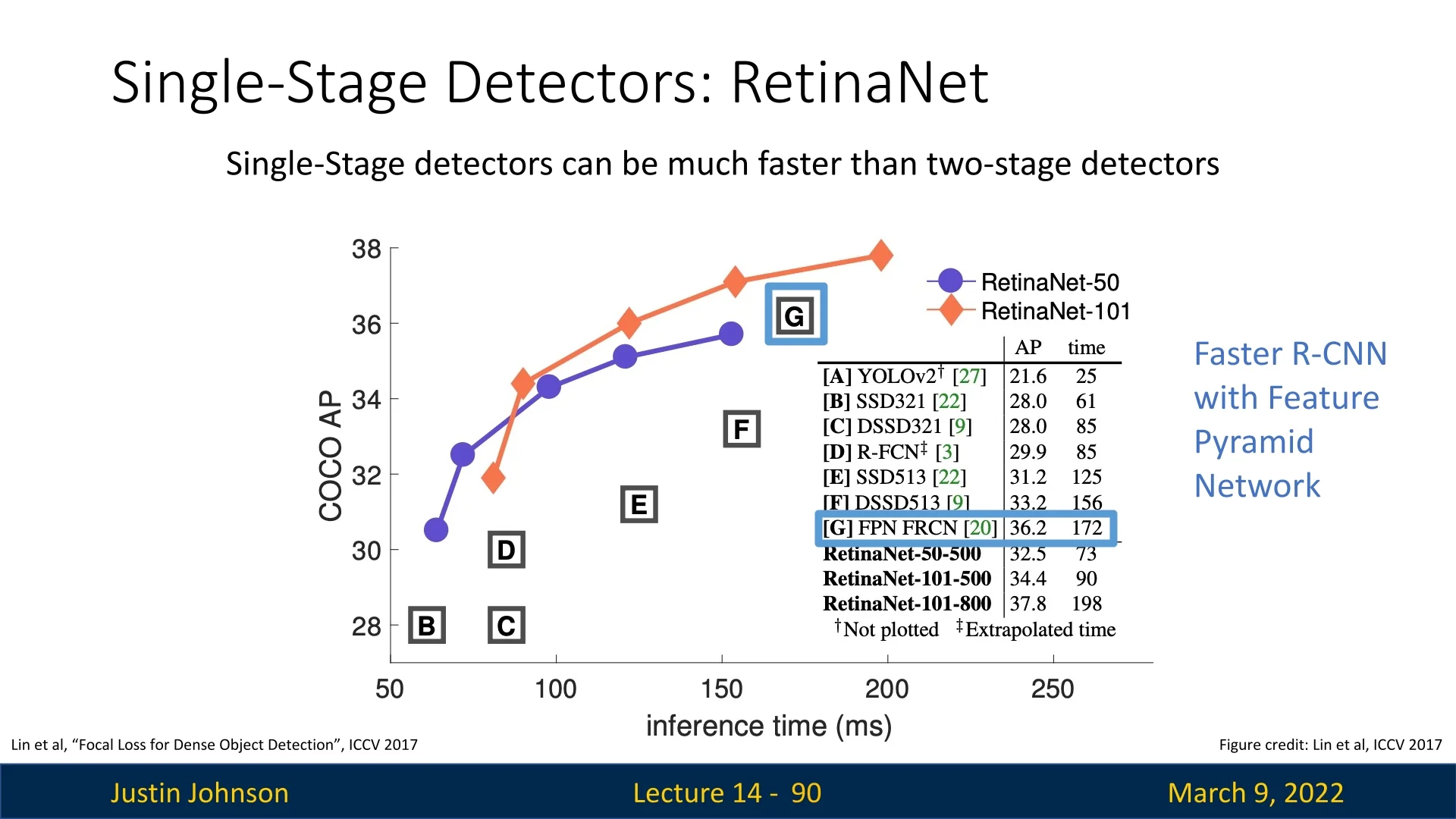
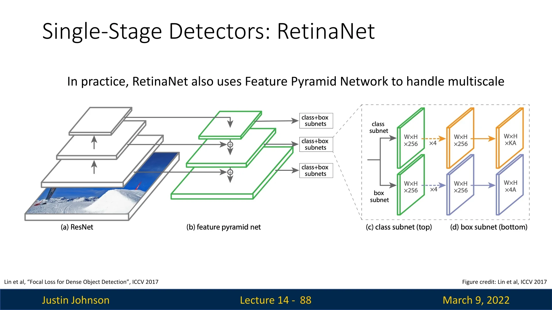
RetinaNet [368] was a major breakthrough in object detection, becoming the first single-stage detector to surpass the performance of top two-stage methods such as Faster R-CNN. It is based on a ResNet-101-FPN or ResNeXt-101-FPN backbone, where the Feature Pyramid Network (FPN) serves as the neck. By leveraging FPN, RetinaNet effectively handles multi-scale object detection while maintaining high efficiency.
14.4.1 Why Single-Stage Detectors Can Be Faster
Single-stage object detectors predict object categories and bounding boxes directly from feature maps, eliminating the need for a region proposal step. Unlike Faster R-CNN, which processes only a few thousand region proposals per image, single-stage detectors like RetinaNet operate on a dense grid of anchor boxes—potentially processing over 100,000 candidate regions in a single forward pass.
- Efficiency: Instead of applying a second-stage classifier per proposal, RetinaNet classifies objects in a single step, reducing inference time.
- Parallelization: Since all predictions are made in parallel, one-stage detectors can fully utilize modern hardware like GPUs.
However, despite these advantages, single-stage detectors historically struggled with class imbalance, which RetinaNet successfully addresses.
14.4.2 The Class Imbalance Problem in Dense Detection
One of the main challenges in single-stage detection is extreme foreground–background class imbalance. Because these detectors make predictions densely over the entire feature map, they evaluate tens of thousands (sometimes over 100,000) of anchors per image, while only a tiny fraction of them actually overlap a ground-truth object.
Concretely, this means that the vast majority of anchors are easy background examples. This imbalance causes two related problems:
- 1.
- Inefficient training: Most negative anchors are trivial to classify as background, so their individual loss and gradients are very small. Yet they still consume most of the computation in each forward/backward pass. The network spends a lot of effort repeatedly confirming “this is background” instead of learning from the relatively few informative foreground examples and hard negatives.
- 2.
- Domination of the loss by easy negatives: Although each easy background anchor contributes only a tiny loss, their sheer quantity means their summed contribution can overwhelm the loss from the few positive anchors. In this regime, a degenerate solution that simply predicts “background” almost everywhere can achieve low average loss and high raw accuracy, while completely failing to detect objects (very low recall). The optimizer is therefore biased toward modeling the majority background class well, rather than learning strong features for the rare foreground class.
This issue is much less severe in two-stage detectors like Faster R-CNN, where the RPN filters out most background regions before the second-stage classifier, leaving a more balanced subset of positive and negative proposals for training.
RetinaNet’s key contribution is to tackle this imbalance at the loss level, introducing the Focal Loss to down-weight easy negatives so that training focuses on the scarce, informative examples.
14.4.3 Focal Loss: Addressing Class Imbalance
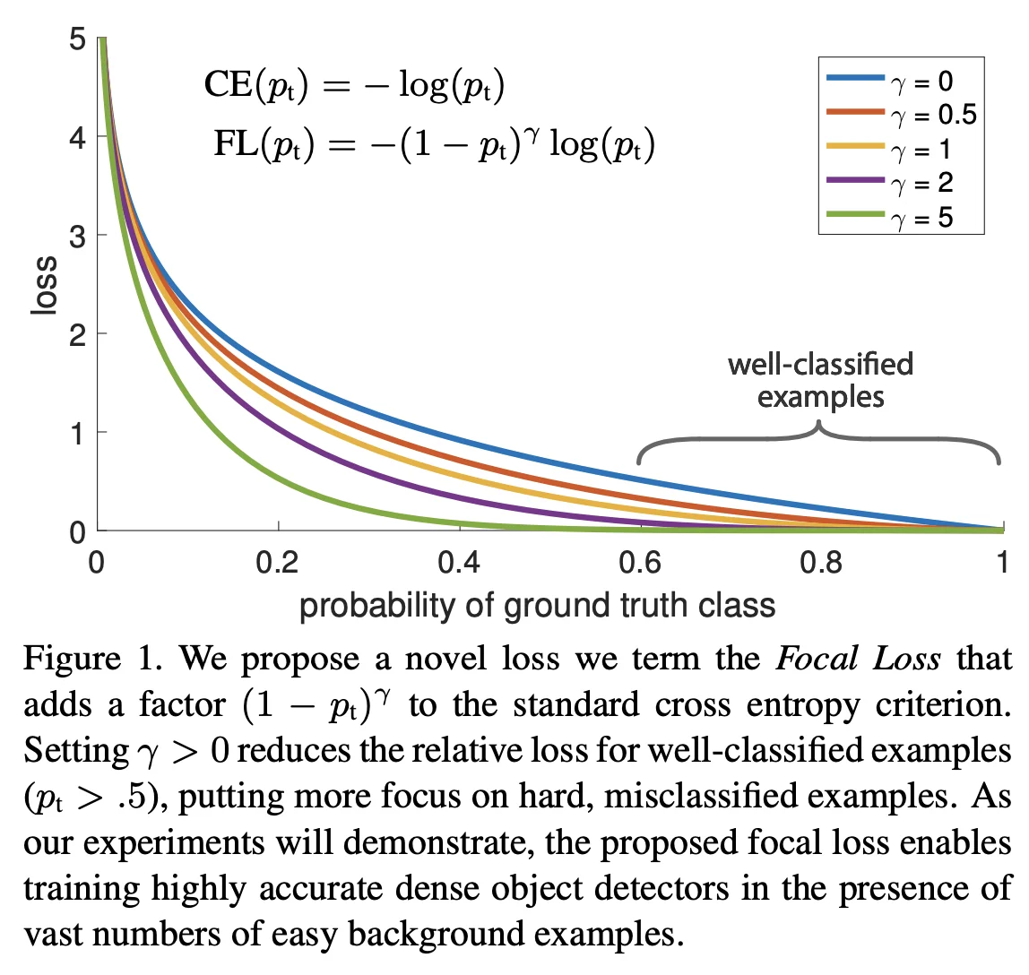
RetinaNet introduced the focal loss to tackle the severe class imbalance inherent in one-stage detectors. Instead of resorting to heuristic sampling or hard-negative mining, focal loss modifies the standard cross-entropy (CE) loss by down-weighting the loss contribution of well-classified examples, thereby shifting the model’s focus toward hard, misclassified examples.
The focal loss is defined as:
\[ FL(p_t) = - (1 - p_t)^\gamma \log (p_t) \]
where:
- \( p_t \) is the predicted probability for the ground-truth class.
- \( \gamma \) is the tunable focusing parameter.
For comparison, the standard cross-entropy loss is:
\[ CE(p_t) = -\log (p_t) \]
By introducing the modulating factor \((1-p_t)^\gamma \), the focal loss reduces the loss for examples that are already well-classified (i.e., when \( p_t \) is high). For instance, with \(\gamma = 2\):
- If \( p_t = 0.9 \), then \((1-0.9)^2 = 0.01\), and the loss becomes approximately \(0.01 \times -\log (0.9) \approx 0.01 \times 0.105 = 0.00105\). In contrast, the standard CE loss would be about 0.105.
- If \( p_t = 0.5 \), then \((1-0.5)^2 = 0.25\), and the loss is \(0.25 \times -\log (0.5) \approx 0.25 \times 0.693 = 0.173\).
- If \( p_t = 0.2 \), then \((1-0.2)^2 = 0.64\), and the loss is \(0.64 \times -\log (0.2) \approx 0.64 \times 1.609 = 1.029\).
These examples illustrate that as the prediction confidence \( p_t \) increases (i.e., for easy examples), the modulating factor quickly shrinks the loss, allowing the model to focus its learning capacity on the hard examples where \( p_t \) is lower.
An \(\alpha \)-balanced variant of the focal loss can further address class imbalance by assigning different weights to positive and negative examples:
\[ FL(p_t) = -\alpha _t (1 - p_t)^\gamma \log (p_t) \]
Here, \(\alpha _t\) is chosen to down-weight the loss for the dominant class (usually the background). In practice, selecting \(\gamma = 2\) and an appropriate \(\alpha \) (e.g., 0.25) has been shown to yield robust results.
In summary, focal loss is a key innovation in RetinaNet that directly addresses class imbalance by dynamically down-weighting the loss from easy examples. This enables training a dense one-stage detector effectively without resorting to complex sampling heuristics, ultimately achieving state-of-the-art accuracy while maintaining fast inference speeds.
14.4.4 RetinaNet Architecture and Pipeline
Backbone and Neck (FPN) RetinaNet uses a standard ImageNet–pretrained backbone (e.g., ResNet-50/101 or ResNeXt-101) to produce a hierarchy of feature maps (commonly denoted \(C_3,C_4,C_5\)). Early backbone stages are high-resolution but semantically weaker; late stages are semantically strong but very coarse. The Feature Pyramid Network (FPN) is a lightweight top-down pathway with lateral connections that fuses these signals to create a new set of semantically strong, multi-scale maps \(P_3,\dots ,P_7\). Concretely:
- \(P_5\) is obtained from \(C_5\) by a \(1{\times }1\) lateral conv; \(P_4\) and \(P_3\) are formed by upsampling the higher level and adding a lateral projection from \(C_4\) and \(C_3\) respectively, followed by a \(3{\times }3\) conv for smoothing.
- \(P_6\) and \(P_7\) extend the pyramid for very large objects via stride-2 \(3{\times }3\) convs (e.g., \(P_6\) directly from \(C_5\), then \(P_7\) from \(P_6\) with a ReLU in between).
Each level has a well-defined stride relative to the input image, typically \(\{8,16,32,64,128\}\) pixels for \(P_3\)–\(P_7\). Thus, one spatial location at \(P_\ell \) summarizes roughly a \(\mbox{stride}_\ell \times \mbox{stride}_\ell \) patch of the input. High-resolution \(P_3\) captures small objects; low-resolution \(P_6,P_7\) capture large ones and global context.
Dense Anchors (per FPN level) Detection is made dense by tiling anchors—predefined box prototypes—at every spatial location of every pyramid level. RetinaNet assigns each level a base side length \[ s_\ell \in \{32,64,128,256,512\}\quad \mbox{for}\quad P_3,\dots ,P_7, \] so that level \(P_\ell \) is responsible for objects whose side lengths are \(\mathcal {O}(s_\ell )\). To cover shapes and nearby scales without exploding the search space, \(\mathbf {A=9}\) anchors are placed per location by combining \[ \mbox{aspect ratios } r \in \{1/2,\,1,\,2\}\quad \mbox{and}\quad \mbox{in-octave scales } m_k \in \{2^{0},\,2^{1/3},\,2^{2/3}\}. \] Given \((s_\ell ,m_k,r)\), an anchor’s width and height are \[ w_{\ell ,k,r} = s_\ell \, m_k\, \sqrt {r},\qquad h_{\ell ,k,r} = s_\ell \, m_k\, / \sqrt {r}, \] which preserves the anchor’s area near \((s_\ell m_k)^2\) while adjusting its shape by \(r=w/h\).
Why fractional scales like \(2^{1/3}\)? RetinaNet partitions each octave (a doubling of size) into three equal steps in \(\log _2\) space. The multiplicative ratio between adjacent scales is \(2^{1/3}\approx 1.26\). This yields anchors that (i) are evenly spaced in scale (no “holes” between \(32\) and \(64\), etc.), (ii) avoid redundant near-duplicates that arise with coarse integer jumps, and (iii) keep coverage smooth across object sizes. Intuitively, if an object’s true size lies between powers of two, one of the three in-octave scales will land close enough that the regressor only needs to make a small, stable adjustment.
Across \(P_3\)–\(P_7\), this construction spans effective side lengths from roughly \(32\) to \(512\) pixels (and intermediate in-octave values), producing on the order of \(10^5\) anchors per image—ample coverage for size and shape, while remaining efficient due to shared convolutions over the pyramid.
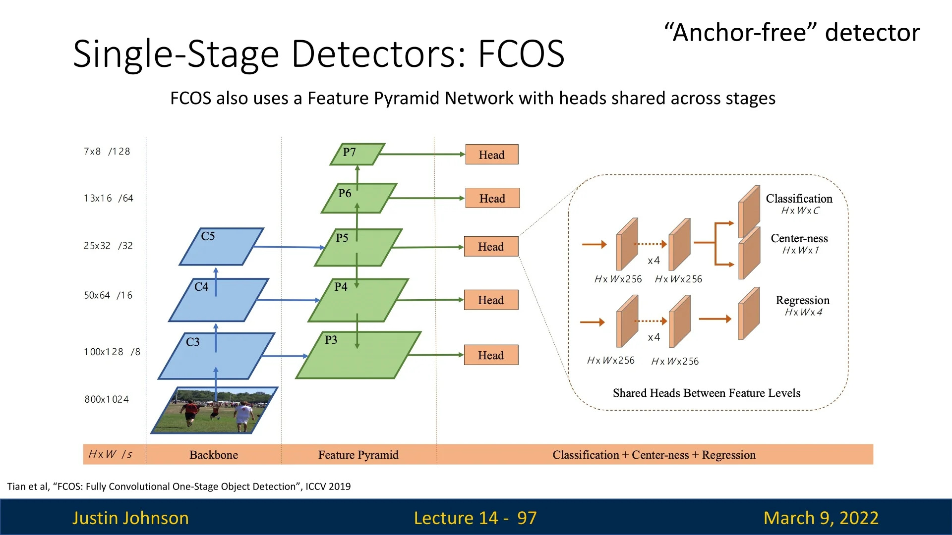
RetinaNet attaches two small, fully convolutional “heads” to every FPN level; their weights are shared across levels for parameter efficiency (the two heads do not share weights with each other):
- Classification head: a subnetwork of four \(3\times 3\) conv layers with 256 channels (each followed by ReLU), ending in a \(3\times 3\) conv that outputs \(A\times C\) per-class logits per spatial location. A sigmoid is applied independently to each of the \(C\) classes (no softmax over classes), which pairs naturally with the Focal Loss.
- Box regression head: an identically shaped subnetwork that ends in \(A\times 4\) outputs per location, parameterizing relative offsets \((t_x,t_y,t_w,t_h)\) from the anchor.
Bias initialization for stability. To counter the extreme initial imbalance, RetinaNet initializes the final classification-layer bias to \[ b=-\log \!\left (\frac {1-\pi }{\pi }\right ),\quad \pi =0.01, \] so the network starts with a low prior probability for foreground, reducing spurious early gradients from the vast background set.
Inference (single pass) All FPN levels are processed in parallel, producing a total of \(\mathcal {O}(10^5)\) anchor predictions per image. After a low score threshold (e.g., 0.05), RetinaNet applies per-class NMS (e.g., IoU 0.5) and keeps the top-\(K\) detections (e.g., \(K{=}100\)).
Why this works (and what was missing before) Architecturally, RetinaNet is deliberately simple: it keeps the RPN’s efficient, fully convolutional template but upgrades to multi-class classification and full box refinement over a feature pyramid. The historical blocker for single-stage accuracy was not the architecture but the extreme class imbalance inherent to dense prediction. RetinaNet’s breakthrough is to pair this streamlined design with the Focal Loss, which down-weights the flood of easy negatives so the classifier learns from scarce positives and hard examples. The result is two-stage–level accuracy with single-stage speed.
14.5 FCOS: An Anchor-Free, Fully Convolutional Detector
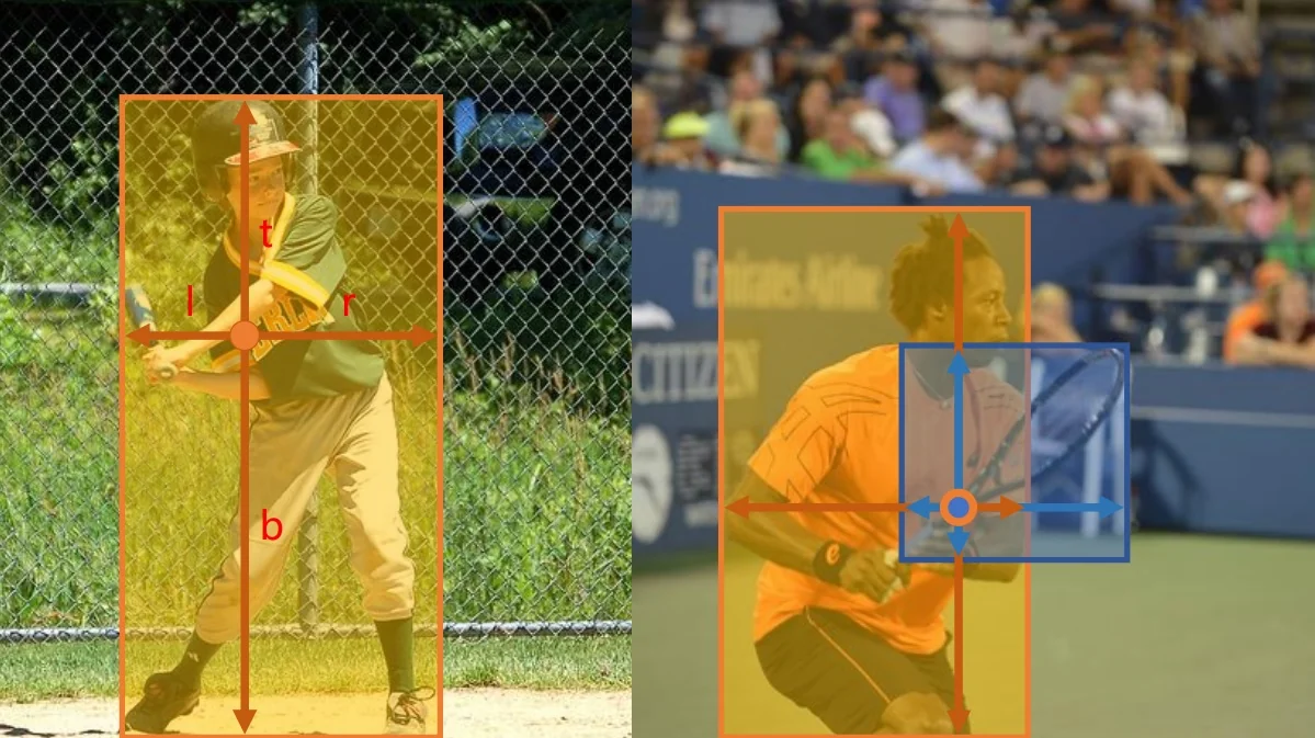
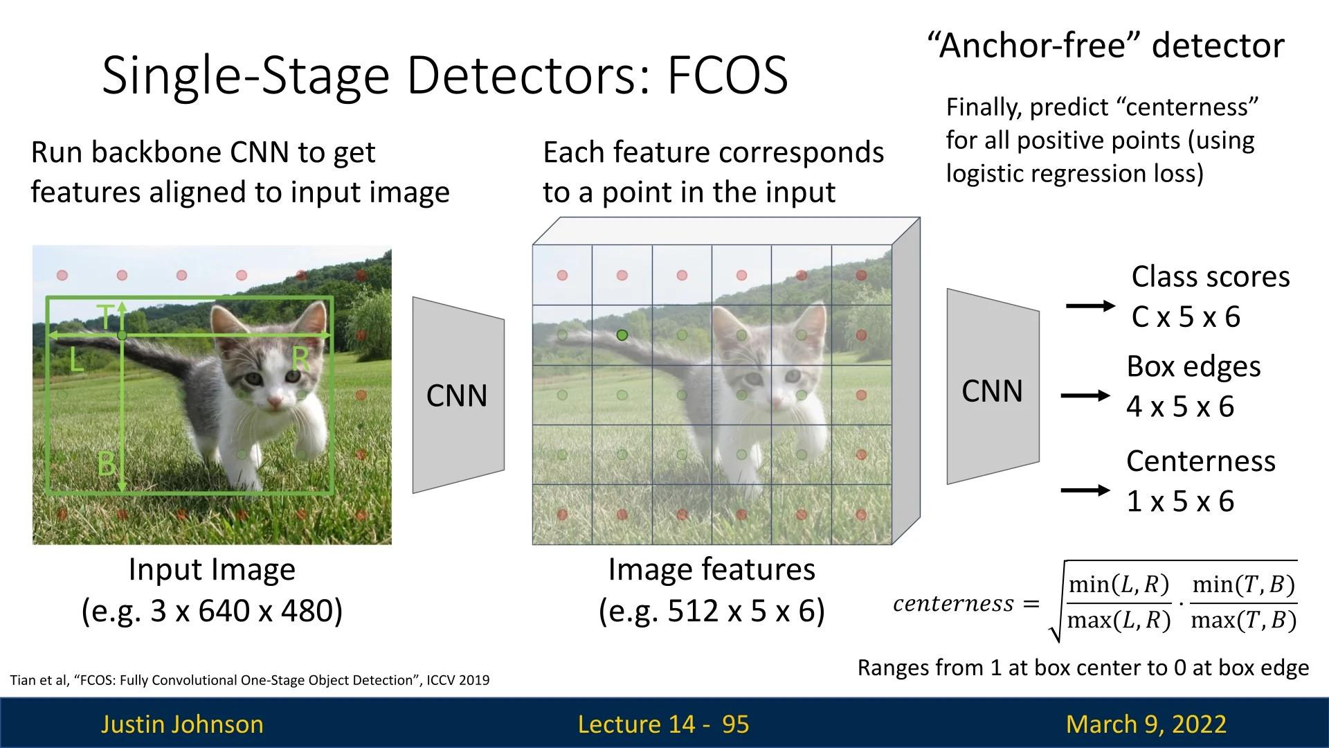
FCOS [637] is an anchor-free one-stage detector that casts detection as a dense, per-pixel prediction problem. Instead of matching ground-truth boxes to a large, hand-designed set of anchors (sizes, aspect ratios, and assignment rules), every spatial location on a feature map can vote for an object by predicting its class and the distances from that location to the four sides of the object’s box. This removes anchor hyperparameters and simplifies both the design and the training pipeline.
14.5.1 Core Pipeline and Supervision
Backbone and Feature Maps A backbone (e.g., ResNet) with FPN produces a pyramid of feature maps \(\{P_3,\dots ,P_7\}\). A location \((x,y)\) on a pyramid level with stride \(s\) corresponds to an input coordinate \(\tilde {x}=x\cdot s+\delta ,\ \tilde {y}=y\cdot s+\delta \) (with a fixed offset \(\delta \) such as \(s/2\)).
Positive/Negative Assignment For each feature-map location, FCOS checks whether its mapped coordinate \((\tilde {x},\tilde {y})\) lies inside any ground-truth box \(B=(x_0,y_0,x_1,y_1)\). If not, the location is negative (background). If yes, it is positive and is assigned to (i) that class and (ii) a single box, chosen as the smallest-area box among those covering \((\tilde {x},\tilde {y})\) to favor supervision from small, harder objects.
Distance-From-Point Regression Targets For a positive location, regression targets are the distances to the four sides of its assigned box: \[ l^\ast =\tilde {x}-x_0,\quad t^\ast =\tilde {y}-y_0,\quad r^\ast =x_1-\tilde {x},\quad b^\ast =y_1-\tilde {y}. \] At inference, predicted distances \((l,t,r,b)\) are converted back to a box \((\tilde {x}-l,\ \tilde {y}-t,\ \tilde {x}+r,\ \tilde {y}+b)\).
14.5.2 Multi-Level Prediction with FPN
As in RetinaNet, FCOS uses FPN to divide the problem by object size rather than by anchor scale. Each level is responsible for a range of object sizes (typical choices): \[ \begin {aligned} P_3 &: (0,64]\ \mbox{pixels},\quad P_4 &: (64,128],\quad P_5 &: (128,256],\\ P_6 &: (256,512],\quad P_7 &: (512,\infty ) \end {aligned} \] This assignment reduces label ambiguity across scales and lets a single set of prediction heads operate reliably at all pyramid levels.
14.5.3 Centerness: Definition, Role, and Intuition
Why Centerness Any location inside a ground-truth box is a valid positive, but locations near the edges tend to yield lower-quality boxes: one or more distances \((l^\ast ,t^\ast ,r^\ast ,b^\ast )\) are small on one side and large on the other, making the regression ill-conditioned. FCOS introduces a third head that predicts a centerness score to quantify how central a location is w.r.t. its assigned object.
Target and Shape The centerness target is \[ \mbox{centerness}^\ast = \sqrt { \frac {\min (l^\ast ,r^\ast )}{\max (l^\ast ,r^\ast )} \cdot \frac {\min (t^\ast ,b^\ast )}{\max (t^\ast ,b^\ast )} }. \] It is the geometric mean of horizontal and vertical “balancedness.” At the exact center, \(l^\ast =r^\ast \) and \(t^\ast =b^\ast \), so \(\mbox{centerness}^\ast =1\). As a point drifts toward an edge on either axis, the corresponding ratio shrinks toward \(0\), and so does the score. The square root moderates the decay so that moderately off-center locations are not over-penalized.
- Training: The centerness head is trained with a binary cross-entropy loss to regress \(\mbox{centerness}^\ast \). In addition, FCOS weights the localization loss of a positive location by \(\mbox{centerness}^\ast \), down-weighting inherently low-quality positives (near edges) during box regression.
- Inference: The final detection confidence is \(\mbox{score} = \mbox{class_prob} \times \mbox{centerness}\). This suppresses spurious boxes predicted from peripheral locations without requiring extra post-processing heuristics.
14.5.4 Localization with IoU Loss
Computation in Distance Parameterization Let the predicted distances be \((l,t,r,b)\) and the targets \((l^\ast ,t^\ast ,r^\ast ,b^\ast )\) for the same positive location. Define predicted and target areas \[ A_p=(l+r)(t+b),\qquad A_g=(l^\ast +r^\ast )(t^\ast +b^\ast ). \] Because both boxes are anchored at the same location, the intersection width and height are \[ w_I=\min (l,l^\ast )+\min (r,r^\ast ),\qquad h_I=\min (t,t^\ast )+\min (b,b^\ast ), \] and the intersection area is \(A_I=w_I\cdot h_I\). The IoU is \[ \mbox{IoU}=\frac {A_I}{A_p+A_g-A_I},\qquad L_{\mbox{reg}}=-\log (\mbox{IoU})\ \ \mbox{or}\ \ 1-\mbox{IoU}. \]
Why IoU, not \(L_1\) IoU loss is scale-invariant and holistic: it couples all four distances to maximize overlap. In contrast, \(L_1\)/smooth-\(L_1\) penalize each side independently and over-weight large boxes. Variants such as GIoU/DIoU/CIoU can further stabilize optimization, but vanilla IoU already yields strong localization in FCOS.
14.5.5 Multi-Task Objective and Training Scheme
Per image, let \(\mathcal {P}\) be the set of positive locations across all pyramid levels and \(N_+\!=\!|\mathcal {P}|\) (with a small \(\epsilon \) to avoid division by zero). FCOS minimizes \[ L_{\mbox{total}} =\underbrace {L_{\mbox{cls}}}_{\mbox{focal, pos+neg}} +\lambda _{\mbox{reg}} \underbrace {\frac {1}{N_+}\sum _{i\in \mathcal {P}}\mbox{centerness}_i^\ast \,L_{\mbox{reg},i}}_{\mbox{IoU on positives, weighted by } \mbox{centerness}^\ast } +\lambda _{\mbox{ctr}} \underbrace {\frac {1}{N_+}\sum _{i\in \mathcal {P}} \mbox{BCE}(\hat {c}_i,\mbox{centerness}_i^\ast )}_{\mbox{centerness head on positives}}, \] where:
- \(L_{\mbox{cls}}\) is the Focal Loss over all locations (positives and negatives), mitigating extreme foreground–background imbalance
- \(L_{\mbox{reg}}\) is the IoU loss in the distance parameterization for positives only
- The regression term is weighted by \(\mbox{centerness}^\ast \) to de-emphasize inherently low-quality edge positives
- \(\lambda _{\mbox{reg}},\lambda _{\mbox{ctr}}\) balance localization and centerness terms; practical defaults often set them to \(1\)
At inference, the per-class probability is multiplied by the predicted centerness before NMS. Thus, focal loss addresses class imbalance, IoU loss optimizes overlap quality, and centerness calibrates both training weights (for localization) and test-time confidences.
14.5.6 Inference
Single forward pass over the FPN yields class scores, distances, and centerness for every location. Predictions with low class score are filtered; remaining scores are multiplied by centerness; distances are converted to boxes; per-class NMS produces final detections.
14.5.7 Advantages of FCOS
FCOS introduces several improvements over anchor-based detectors:
- Simpler Design: Eliminates the need for anchor boxes, reducing hyper-parameter tuning.
- Computational Efficiency: Avoids anchor box computations, reducing memory and processing overhead.
- Better Foreground Utilization: Unlike anchor-based methods, which only consider a subset of anchors, FCOS treats every feature map location inside a ground-truth box as a positive sample.
- Improved Detection Quality: The centerness mechanism suppresses low-quality predictions, reducing false positives.
By leveraging fully convolutional architectures and eliminating the complexities of anchor boxes, FCOS provides a simple yet powerful alternative to traditional object detection methods.
Enrichment 14.6: YOLO - You Only Look Once
Enrichment 14.6.1: Background
YOLO (You Only Look Once) revolutionized object detection by treating it as a single regression problem, enabling real-time detection without requiring multiple passes over an image.
First introduced by Redmon et al. in [534], YOLO has continuously evolved (from YOLOv1 to more advanced versions) by improving accuracy while maintaining real-time performance. Its success stems from:
- Speed: YOLO’s one-pass approach makes it significantly faster than two-stage detectors, enabling applications in autonomous driving, surveillance, and real-time video analysis.
- Global Reasoning: By processing the entire image at once, YOLO reduces false positives from overlapping region proposals and makes more context-aware predictions.
Thanks to these advantages, YOLO remains one of the most widely used object detection frameworks, consistently setting new benchmarks for real-time applications.
Enrichment 14.6.2: Step-by-Step: How YOLOv1 Processes an Input Image
YOLOv1 (You Only Look Once) is a single-stage object detector that predicts bounding boxes and class probabilities in one unified forward pass. Below, we outline how YOLOv1 processes an image from start to finish.
1. Input Image and Preprocessing
- Dimensions: YOLOv1 typically expects an image resized to \(448\times 448\).
- Normalization: In practice, pixel values may be scaled (e.g., to \([0,1]\) or \([-1,1]\)) to help training stability.
- This preprocessed image is fed into the network as a PyTorch Tensor
of shape
\(\bigl [\mbox{batch_size}, 3, 448, 448\bigr ]\).
2. Feature Extraction (DarkNet + Additional Convolution Layers) YOLOv1 is composed of:
- 1.
- DarkNet, which produces a high-level feature map from the input image. DarkNet is a series of convolutional layers interspersed with activations (Leaky ReLU) and sometimes batch normalization.
- 2.
- Additional convolution layers that further refine the 1024-channel output of DarkNet.
Eventually, these convolutions yield a feature map of shape \(\bigl [\mbox{batch_size}, 1024, S, S\bigr ]\), where S is grid dimension, a hyperparameter that fits our feature extraction process (in YOLOv1, \(S=7\)). Hence, YOLOv1 divides the image conceptually into a \(7\times 7\) grid.
3. Flattening and Fully Connected Layers After the final convolutional layer, the 7\(\times \)7\(\times \)1024 feature map is:
- Flattened into a 1D vector of length \(7 \times 7 \times 1024 = 50176\).
- Passed into a Linear(50176, 4096) layer, a Leaky ReLU, and a dropout layer.
-
Finally, passed into a linear output layer of size \(S \times S \times (5B + C)\), where:
- \(S=7\) is the number of grid cells per dimension.
- \(B=2\) is the number of bounding boxes each cell predicts.
- \(C=20\) is the number of classes (for the PASCAL VOC Dataset).
This yields an output tensor of shape: \[ \bigl [\mbox{batch_size},\,7,\,7,\,(5 \times 2 + 20)\bigr ] = \bigl [\mbox{batch_size},\,7,\,7,\,30\bigr ]. \] The final layer is linear: it produces real-valued outputs that are trained, via a sum-of-squared-errors loss, to approximate normalized targets (e.g., coordinates and confidences in \([0,1]\)).
4. Understanding the Output Format Concretely, each cell’s part of the final output includes:
- 1.
- \(\mathbf {(x, y)}\): Center offsets for box 1 within the cell, in \([0,1]\).
- 2.
- \(\mathbf {w, h}\): Width and height for box 1, also in \([0,1]\).
- 3.
- \(\mbox{confidence}\): A single scalar in \([0,1]\) for how likely the predicted box is valid (the bounding box overlaps an object).
- 4.
- The same 5 parameters for box 2 (\(x, y, w, h, \mbox{confidence}\)).
- 5.
- \(\mathbf {C}\) class probabilities for the cell, also in \([0,1]\).
5. Parameterization and Normalization Although the final layer is linear, YOLOv1 parametrizes its targets so that most predicted quantities naturally lie in \([0,1]\):
- \(\hat {x}, \hat {y}\) are trained to represent the center of the box relative to the grid cell that predicts it, with targets in \([0,1]\). At inference time, we convert them to absolute image coordinates using the cell indices \((c_x, c_y)\) and the grid size \(S\).
- \(\hat {w}, \hat {h}\) are trained to represent the box width and height relative to the full image size, again with targets in \([0,1]\). The loss uses \(\sqrt {w}\) and \(\sqrt {h}\) to emphasize errors on small boxes.
- The confidence output for each box is trained to regress to \[ C = P(\mbox{object}) \cdot \mathrm {IoU}(\mbox{box}, \mbox{gt}) \in [0,1], \] where \(\mathrm {IoU}\) is the intersection-over-union with the ground-truth box.
- The class probabilities are conditional probabilities \(P(\mbox{class}_c \mid \mbox{object})\) at the cell level, with targets given by one-hot vectors over the \(C\) classes.
Thus, even though the network’s outputs are unconstrained real numbers, the combination of normalized targets and an L2 loss encourages them to behave like probabilities and normalized coordinates.
6. Converting Predictions to Actual Bounding Boxes Inside each cell, we do: \[ \hat {x}_\mbox{abs} = \frac {c_x + \hat {x}}{S}, \quad \hat {y}_\mbox{abs} = \frac {c_y + \hat {y}}{S}, \] where \(c_x, c_y\) is the grid cell’s top-left integer index (e.g., \((2,3)\) if we are in row 2, column 3) and \(S=7\). Then, \[ \hat {w}_\mbox{abs} = \hat {w} \times \mbox{image_width}, \quad \hat {h}_\mbox{abs} = \hat {h} \times \mbox{image_height}. \] The bounding box corners become: \[ x_{\mbox{min}} = \hat {x}_\mbox{abs} - \tfrac {\hat {w}_\mbox{abs}}{2}, \quad y_{\mbox{min}} = \hat {y}_\mbox{abs} - \tfrac {\hat {h}_\mbox{abs}}{2}, \quad x_{\mbox{max}} = \hat {x}_\mbox{abs} + \tfrac {\hat {w}_\mbox{abs}}{2}, \quad y_{\mbox{max}} = \hat {y}_\mbox{abs} + \tfrac {\hat {h}_\mbox{abs}}{2}. \] Thus each cell contributes up to \(B=2\) bounding boxes in absolute image coordinates.
7. Loss and Training (High Level) YOLO’s loss function balances three main terms:
- Localization Loss: Penalizes bounding box coordinate errors \((x, y, w, h)\) for the box in each cell that is responsible for an object. The loss uses \(\sqrt {w}\) and \(\sqrt {h}\) to give relatively more weight to small boxes.
- Confidence Loss: Penalizes errors in the objectness confidence. It pushes confidence toward 1 for responsible boxes in cells that contain objects, and toward 0 for all boxes in cells that do not contain objects.
- Classification Loss: A sum-of-squared-errors (L2) loss on the class probabilities, applied only to cells that contain an object.
To balance these contributions, the loss up-weights localization (\(\lambda _{\mbox{coord}} = 5\)) and down-weights the confidence loss for background cells (\(\lambda _{\mbox{noobj}} = 0.5\)).
The full loss function is: \[ L = \lambda _{\mbox{coord}} \sum _{i=1}^{S^2} \sum _{j=1}^{B} 1^{\mbox{obj}}_{ij} \bigl [(x_i - \hat {x}_i)^2 + (y_i - \hat {y}_i)^2\bigr ] \] \[ + \lambda _{\mbox{coord}} \sum _{i=1}^{S^2}\sum _{j=1}^{B} 1^{\mbox{obj}}_{ij} \bigl [(\sqrt {w_i} - \sqrt {\hat {w}_i})^2 + (\sqrt {h_i} - \sqrt {\hat {h}_i})^2\bigr ] \] \[ + \sum _{i=1}^{S^2}\sum _{j=1}^{B} 1^{\mbox{obj}}_{ij} \bigl (C_i - \hat {C}_i\bigr )^2 \] \[ + \lambda _{\mbox{noobj}} \sum _{i=1}^{S^2}\sum _{j=1}^{B} 1^{\mbox{noobj}}_{ij} \bigl (C_i - \hat {C}_i\bigr )^2 \] \[ + \sum _{i=1}^{S^2} 1^{\mbox{obj}}_{i} \sum _{c \in \mbox{classes}} \bigl (p_i(c) - \hat {p}_i(c)\bigr )^2. \]
Here the confidence target for each predicted box is defined as \[ C_i = P(\mbox{object in cell } i) \times \mathrm {IoU}(\mbox{predicted box}, \mbox{ground truth}), \] so that \(C_i = 0\) for cells without objects, and \(C_i\) equals the IoU for the “responsible” box in cells that contain an object. This ties the confidence both to object presence and to localization quality.
8. Why It Works (and Its Trade-offs)
- Efficiency: Only a single CNN forward pass is needed. This is much faster than multi-stage pipelines like R-CNN.
- Grid-Based Reasoning: Each cell “looks” at local features and tries to detect objects centered there, simplifying the logic behind region proposals.
- No Anchors in YOLOv1: The network directly learns bounding box shapes, which can be good for moderate object scale variety, but struggles for extremely small or large aspect ratios. Later YOLO versions added anchor priors for more robust shape handling.
9. Final Detections and NMS Once the forward pass is done, YOLOv1 typically:
- Converts each cell’s bounding box predictions into absolute coordinates as described.
- Filters out boxes with low confidence.
- Applies Non-Maximum Suppression (NMS) to reduce duplicates—keeping only the highest confidence box for each object.
The final set of bounding boxes with class labels becomes YOLO’s detection result.
- 1.
- Input (448\(\times \)448) \(\to \) DarkNet + Conv \(\to \) Flatten \(\to \) Fully Connected (4096D) \(\to \) \(\texttt{Linear}\) \(\to \) \(\texttt{Sigmoid}\).
- 2.
- Output shape: \(\bigl [\mbox{batch_size}, 7, 7, (5 \times 2 + 20)\bigr ]\).
- 3.
- Each \((7\times 7)\) cell: \(\underbrace {x, y, w, h, \mbox{confidence}}_{\mbox{box 1}},\; \underbrace {x, y, w, h, \mbox{confidence}}_{\mbox{box 2}},\; \mbox{class probabilities}\).
- 4.
- \(\sigma (\cdot )\) ensures values in \([0,1]\). The predicted offsets are scaled to the full image, producing final bounding boxes.
- 5.
- Loss includes coordinate errors, objectness confidence errors, and classification errors.
- 6.
- Post-processing merges overlapping boxes (NMS).
This pipeline captures what YOLOv1 does and why it does it in a simple, end-to-end fashion: object localization, classification, and bounding-box regression are all learned jointly in one pass.
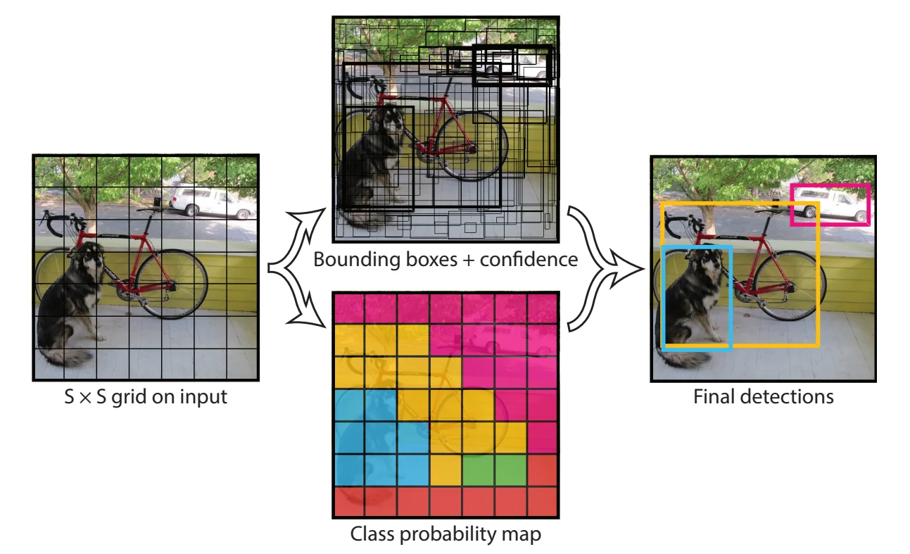
Enrichment 14.6.3: Evolution of YOLO
Over time, multiple versions of YOLO have been developed to address its limitations:
- YOLOv2 (2017) [532]: Introduced anchor boxes, batch normalization, and multi-scale training, improving both accuracy and generalization.
- YOLOv3 (2018) [533]: Added Darknet-53 as a backbone, feature pyramids, and objectness scores, significantly boosting detection accuracy.
- YOLOv4 (2020) [47]: Focused on increasing efficiency with new activation functions (Mish), better data augmentation, and optimization techniques.
- YOLOv5+ (2020s+): Introduced by Ultralytics, leveraging PyTorch and adding modern training techniques such as mosaic augmentation and hyperparameter tuning.
Each version improves upon the previous, refining accuracy, robustness, and efficiency, solidifying YOLO as one of the most influential object detection models in real-time applications.
14.7 Conclusion: The Evolution of Object Detection
Object detection has undergone significant advancements over the years, with each iteration improving both speed and accuracy. This chapter traced the evolution of object detectors, highlighting key innovations that have shaped modern detection frameworks.
From R-CNN to Faster R-CNN: Learning Region Proposals Early object detection models, such as R-CNN, relied on region proposal methods like Selective Search to generate candidate object regions. While effective, R-CNN suffered from slow inference times, as it required passing each region through a CNN separately.
Fast R-CNN improved this process by computing feature maps once for the entire image and then applying RoI Pooling or RoIAlign to extract features for each proposal, significantly reducing inference time. However, it still relied on external region proposals, which remained a computational bottleneck.
Faster R-CNN introduced Region Proposal Networks (RPNs), replacing hand-crafted region proposal methods with a trainable, CNN-based approach. This enabled fully end-to-end training, where the region proposals were learned jointly with the detector. While Faster R-CNN achieved high accuracy, its two-stage nature still made it slower, and also more computationally expensive.
Improving Multi-Scale Detection: Feature Pyramid Networks (FPN) While Faster R-CNN was a breakthrough, it struggled with detecting objects at different scales, especially smaller ones. To address this, Feature Pyramid Networks (FPNs) were introduced, leveraging the multi-scale hierarchical features of CNNs to enhance object detection at different resolutions. By integrating top-down pathways that fused low-level spatial details with high-level semantic information, FPNs became a crucial addition to many detection architectures.
RetinaNet: A Breakthrough for One-Stage Detectors While two-stage detectors like Faster R-CNN were dominant, they were computationally expensive, motivating the need for faster alternatives. RetinaNet was a milestone in object detection as it was the first single-stage detector to surpass two-stage detectors in accuracy, all while maintaining significantly higher speed.
RetinaNet introduced Focal Loss, addressing the issue of class imbalance between foreground and background objects. By down-weighting easy samples and focusing on harder examples, it improved training efficiency and allowed single-stage networks to perform on par with or better than their two-stage counterparts. RetinaNet, like Faster R-CNN, leveraged FPNs for multi-scale feature extraction, making it robust for detecting objects across different sizes.
FCOS: Moving Toward Anchor-Free Detection While RetinaNet and previous detectors relied on anchor boxes (predefined bounding box templates), FCOS took a different approach. It introduced an anchor-free detection framework, treating object detection as a per-pixel regression problem, similar to semantic segmentation. Instead of relying on predefined priors, FCOS predicted bounding boxes directly at each spatial location. This simplified the detection pipeline by removing anchor hyperparameters while maintaining strong performance.
YOLO: A Widely Used Real-Time Detector Parallel to these developments, the YOLO (You Only Look Once) family of detectors emerged as a dominant force in real-time applications. YOLO takes a different approach by treating detection as a global regression problem, dividing the image into a grid and predicting bounding boxes and class probabilities in a single forward pass. Over successive versions, YOLO has been continuously refined for accuracy and efficiency, making it one of the most popular and influential object detection frameworks.
Looking Ahead: Transformers and SOTA Detectors While this chapter focused on CNN-based object detectors, modern detection frameworks have evolved further with transformer-based architectures. Models such as the DEtection TRansformer (DETR) and its variants eliminate explicit region proposal mechanisms and instead treat detection as a set prediction problem using attention. In parallel, strong self-supervised vision transformers (for example, DINOv2) provide powerful backbone representations that can be fine-tuned for detection and segmentation tasks. As we progress in this document, we will explore several examples of state-of-the-art (SOTA) detectors that leverage transformers to push the boundaries of both accuracy and efficiency.
Summary Modern object detection has progressed from region-based CNNs to one-stage and transformer-based architectures:
- R-CNN introduced region-based detection but was very slow.
- Fast/Faster R-CNN amortized feature computation and learned region proposals via RPNs, enabling end-to-end training.
- FPNs added multi-scale feature hierarchies, improving performance on small objects.
- RetinaNet showed that one-stage detectors can match and surpass two-stage accuracy using Focal Loss.
- FCOS and such detectors simplified design by predicting boxes directly at each location.
- The YOLO family popularized real-time, grid-based detection.
- Transformer-based detectors (e.g., DETR) remove proposal stages entirely and rely on attention over image features.
These developments build on one another to yield today’s accurate, efficient, and scalable detection frameworks; later chapters will revisit them in the context of transformer-based vision models.
Enrichment 14.8: Detection Transformer (DeTR)
The Detection Transformer (DeTR) [64] is a seminal work that brought the transformer architecture into the object detection domain. Developed by Facebook AI Research (FAIR), DeTR introduced a novel framework that reformulates object detection as a direct set prediction problem, eliminating many traditional hand-crafted components like anchor boxes, region proposals, and non-maximum suppression (NMS).
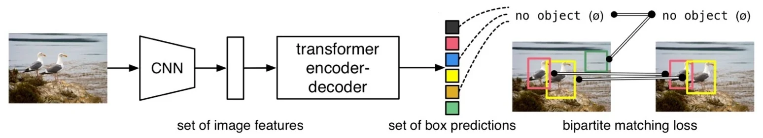
- The input image is first encoded by a convolutional backbone (e.g., ResNet-50), yielding a spatial feature map.
- The flattened feature map is treated as a sequence and passed through a transformer encoder.
- A transformer decoder receives a fixed number \(N\) of learned object queries and produces a corresponding set of \(N\) object predictions.
- Each prediction outputs both a class label and a bounding box.
Why Transformers for Detection? DeTR leverages the global self-attention of transformers to enable long-range dependency modeling across the image. Whereas CNN-based detectors often rely on local context and multi-scale heuristics to infer object presence, transformers can integrate information from the entire image holistically in a single forward pass.
However, this global modeling comes with a key design shift: DeTR produces a fixed-size set of predictions—typically \(N = 100\)—for every image, regardless of how many objects are present. This architectural choice is critical: it allows DeTR to frame detection as a set-to-set matching problem, enabling end-to-end training using a bipartite matching loss.
This design immediately raises a natural question: What happens when the number of actual objects is fewer than \(N\)?
We address this in the next subsection, where we explore how DeTR matches predictions to targets using bipartite matching, and how “no-object” padding plays a central role in the loss function and training dynamics.
Enrichment 14.8.1: Matching Predictions and GT with No-Object Padding
Building on the transformer encoder–decoder and self-attention mechanisms introduced in later chapters, DEtection TRansformer (DETR) [64] revisits object detection as a set prediction problem. Instead of producing a variable number of candidate boxes that must be filtered by anchors and non-maximum suppression (NMS), DETR passes image features through a transformer and predicts a fixed-size set of \(N\) object candidates per image (typically \(N = 100\)), each trained to correspond to at most one object (or a dedicated “no-object” slot).
Challenge: Most images contain fewer than \(N\) objects. This creates a mismatch between the number of predictions and the number of ground-truth annotations (\(M < N\)). How can we supervise all predictions consistently?
Solution: No-Object Padding To address this, DETR pads the ground-truth set with “no-object” entries—placeholder targets that carry a special background class label. The model is trained to recognize these as background predictions.
- Let the image contain \(M\) annotated boxes.
- The padded target set is expanded to size \(N\), by appending \(N - M\) dummy targets with a designated “no-object” class label.
- This allows a one-to-one matching between predicted boxes and targets using the Hungarian algorithm, even when many targets are artificial.
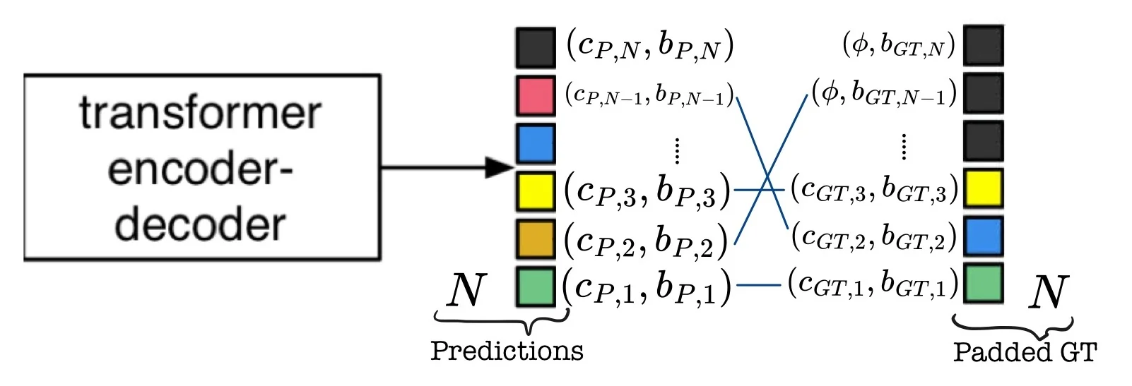
Hungarian Matching: Matching is solved globally using the Hungarian algorithm, which assigns each prediction to exactly one target (real or padded) to minimize the total matching cost:
\[ \mathcal {L}_{\mbox{match}}(i,j) = \lambda _{\mbox{cls}} \cdot \mbox{CE}(\hat {c}_i, c_j) + \lambda _{\mbox{L1}} \cdot \lVert \hat {b}_i - b_j \rVert _1 + \lambda _{\mbox{GIoU}} \cdot \bigl (1 - \mbox{GIoU}(\hat {b}_i, b_j)\bigr ) \]
# Assume:
# targets = List[Dict] with keys ’boxes’ and ’labels’
# num_queries = fixed number of DETR outputs (e.g., 100)
padded_targets = []

for tgt in targets:
boxes = tgt["boxes"]   # [num_objects, 4]
labels = tgt["labels"]  # [num_objects]

num_objs = boxes.size(0)
pad_size = num_queries - num_objs

# Pad with dummy boxes and no-object class label (e.g., 91 for COCO)
padded_boxes = F.pad(boxes,  (0, 0, 0, pad_size))  # [num_queries, 4]
padded_labels = F.pad(labels, (0, pad_size), value=no_object_class)

padded_targets.append({
    "boxes": padded_boxes,
    "labels": padded_labels
})
Why This Matters: This matching-and-padding design:
- Eliminates the need for anchor boxes or NMS.
- Supervises every prediction, even those matched to background.
- Enables fully end-to-end training with standard classification and regression losses.
By framing detection as bipartite matching, DETR achieves a clean and interpretable training objective. In the following subsection, we’ll detail the final loss function and how it combines classification, L1 distance, and GIoU penalties over the matched pairs.
Enrichment 14.8.2: Hungarian Matching Loss and Bounding Box Optimization
After performing bipartite matching between predicted and ground truth boxes (see Enrichment 14.8), DETR computes a loss over these matched pairs to optimize both class predictions and bounding box regressions. This is known as the Hungarian loss, and it operates over a permutation of predictions that minimizes the overall cost.
Step 1: Optimal Bipartite Matching Let the ground truth set be \( y = \{y_1, \dots , y_N\} \), padded with “no-object” entries if the image contains fewer than \( N \) objects. Each element \( y_i = (c_i, b_i) \) contains a class label \( c_i \in \{1, \dots , K\} \cup \{\varnothing \} \) and a bounding box \( b_i \in [0,1]^4 \). Similarly, let \( \hat {y} = \{\hat {y}_1, \dots , \hat {y}_N\} \) be the \( N \) predictions, where each \( \hat {y}_j = (\hat {c}_j, \hat {b}_j) \).
We now seek a permutation \( \hat {\sigma } \in \mathfrak {S}_N \) (the set of all permutations over \( N \) elements) that minimizes the total matching cost:
\[ \hat {\sigma } = \underset {\sigma \in \mathfrak {S}_N}{\arg \min } \sum _{i=1}^N \mathcal {L}_\mbox{match}(y_i, \hat {y}_{\sigma (i)}). \]
This permutation defines a unique one-to-one mapping between each ground truth box and a model prediction.
Step 2: Matching Cost Definition The pairwise cost function accounts for classification and box quality:
\[ \mathcal {L}_\mbox{match}(y_i, \hat {y}_{\sigma (i)}) = -\ind _{\{c_i \neq \varnothing \}} \cdot \hat {p}_{\sigma (i)}(c_i) + \ind _{\{c_i \neq \varnothing \}} \cdot \mathcal {L}_\mbox{box}(b_i, \hat {b}_{\sigma (i)}), \]
where:
- \( \hat {p}_{\sigma (i)}(c_i) \) is the predicted probability for class \( c_i \),
- \( \mathcal {L}_\mbox{box} \) is a bounding box regression loss (see below),
- \( \ind \) denotes the indicator function (equal to 1 when the condition holds, 0 otherwise).
The indicator ensures that background (\( c_i = \varnothing \)) entries do not contribute to the loss.
Step 3: Final Loss Computation Once the optimal matching \( \hat {\sigma } \) is found, the Hungarian loss is computed as:
\[ \mathcal {L}_\mbox{Hungarian}(y, \hat {y}) = \sum _{i=1}^N \left [ - \log \hat {p}_{\hat {\sigma }(i)}(c_i) + \ind _{\{c_i \neq \varnothing \}} \cdot \mathcal {L}_\mbox{box}(b_i, \hat {b}_{\hat {\sigma }(i)}) \right ]. \]
In practice, DETR downweights the classification loss for no-object classes by a factor of 10 to reduce class imbalance effects.
Bounding Box Loss: Smooth L1 and GIoU Components Once a ground truth box \( b_i \) is matched with a predicted box \( \hat {b}_{\sigma (i)} \) (via the Hungarian algorithm), DETR computes a localization loss that balances numerical precision and spatial alignment. This is achieved through a combination of Smooth L1 (Huber) loss and Generalized IoU (GIoU) loss.
1. Smooth L1 Loss (Huber Variant) The Smooth L1 loss—also known as the Huber loss—is a robust alternative to standard L1 or L2 losses. It behaves like an L2 loss near zero (ensuring smooth gradients) and like an L1 loss for larger errors (ensuring robustness to outliers). Formally:
\[ \mbox{SmoothL1}(x) = \begin {cases} 0.5 \cdot \frac {x^2}{\beta }, & \mbox{if } |x| < \beta \\ |x| - 0.5 \cdot \beta , & \mbox{otherwise} \end {cases} \]
The hyperparameter \( \beta \) controls the transition point between the quadratic and linear regimes. For DETR, \( \beta = 1.0 \) is typically used. This makes the box regression more stable, especially during early training.
# Smooth L1 (Huber) loss for bounding box regression
import torch.nn.functional as F

smooth_l1 = F.smooth_l1_loss(
    pred_boxes, target_boxes,
    reduction="none", beta=1.0
)
Despite being a coordinate-wise loss, Smooth L1 doesn’t account for the box’s spatial shape or overlap. This is where GIoU comes in.
2. Generalized IoU (GIoU) Loss Intersection over Union (IoU) is a classic metric for bounding box overlap: \[ \mbox{IoU}(A, B) = \frac {|A \cap B|}{|A \cup B|}. \] However, IoU suffers from a key weakness: if two boxes do not overlap, IoU is 0, providing no learning signal—regardless of how close the boxes are spatially.
To overcome this, [544] proposed the Generalized IoU (GIoU):
\[ \mbox{GIoU}(A, B) = \mbox{IoU}(A, B) - \frac {|C \setminus (A \cup B)|}{|C|}, \] where \( C \) is the smallest enclosing box that fully contains both \( A \) and \( B \). This makes GIoU sensitive to the spatial distance between non-overlapping boxes.
- \( C \) is found by taking the tightest box covering both \( A \) and \( B \), using min and max operations over the corners.
- When \( A \) and \( B \) overlap perfectly, GIoU reduces to IoU.
- When \( A \cap B = \emptyset \), GIoU is negative, providing a gradient toward reducing their separation.
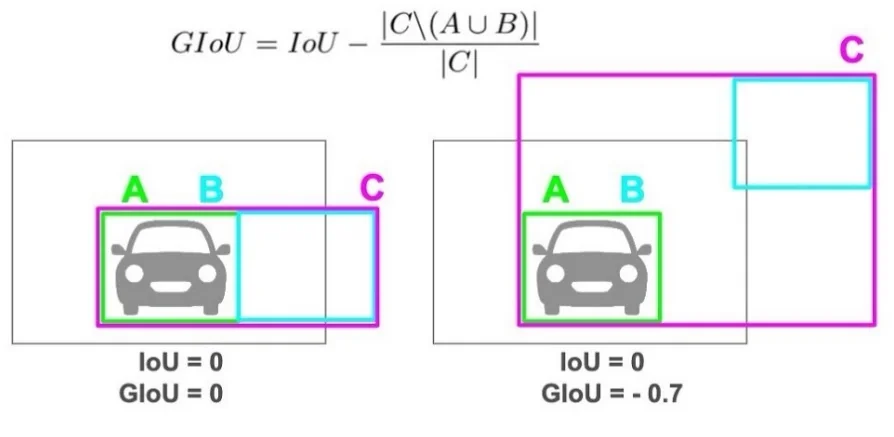
from torchvision.ops import generalized_box_iou

# GIoU loss: 1 - GIoU score
giou = generalized_box_iou(pred_boxes, target_boxes)
giou_loss = 1.0 - giou
3. Combining Smooth L1 and GIoU Each loss captures a different notion of box quality:
- Smooth L1 (Huber): Enforces numerical closeness between box coordinates (good for center, width, height alignment).
- GIoU: Encourages spatial alignment and overlap—especially helpful when predictions are far from the target.
DETR combines the two: \[ \mathcal {L}_\mbox{box}(b_i, \hat {b}_{\sigma (i)}) = \lambda _\mbox{L1} \cdot \mbox{SmoothL1}(b_i, \hat {b}_{\sigma (i)}) + \lambda _\mbox{GIoU} \cdot \left (1 - \mbox{GIoU}(b_i, \hat {b}_{\sigma (i)})\right ), \] where \( \lambda _\mbox{L1}, \lambda _\mbox{GIoU} \) are loss weights (e.g., 5.0 and 2.0 in the DETR paper).
Conclusion By blending coordinate-wise error with geometric overlap, DETR ensures that the model:
- Learns to predict numerically accurate box coordinates,
- Gains spatial awareness even when predictions are initially far off,
- Receives informative gradients during all training phases.
This elegant combination supports DETR’s end-to-end detection approach. Now that we’ve explored how predictions are matched and optimized via loss functions, we proceed to examine the architecture and flow of DETR, from feature extraction to transformer decoding and output prediction.
Enrichment 14.8.3: Architecture Overview
DETR integrates convolutional and transformer-based modules in an end-to-end object detection pipeline. The overall architecture consists of:
- 1.
- A convolutional backbone (e.g., ResNet-50 or ResNet-101) that extracts dense visual features.
- 2.
- A transformer encoder-decoder that models global interactions and predicts \(N\) object candidates.
- 3.
- A bipartite matching and loss computation mechanism to supervise predictions (see Enrichment 14.8.1).
1. CNN Backbone The input image \( X \in \mathbb {R}^{3 \times H_0 \times W_0} \) passes through a CNN backbone (e.g., ResNet-50), producing an activation map: \[ f \in \mathbb {R}^{C \times H \times W}, \quad \mbox{where } C = 2048,\quad H = H_0 / 32,\quad W = W_0 / 32. \] These activations represent coarse spatial features extracted by the CNN. A \(1 \times 1\) convolution reduces the channel dimension from \(C\) to \(d = 256\), yielding \(d\)-dimensional patch embeddings. These are then flattened into a sequence of \(HW\) tokens, each representing a spatial location.
2. Transformer Encoder Each of the \(HW\) flattened patch vectors is enriched with a 2D sine/cosine positional encoding and then passed through a standard transformer encoder (multi-head self-attention + MLP with residuals and LayerNorm). Unlike NLP models (e.g., BERT, GPT), DETR uses longer sequences (\(HW \approx 900\)) but with smaller hidden size (\(d = 256\)) to accommodate memory constraints.
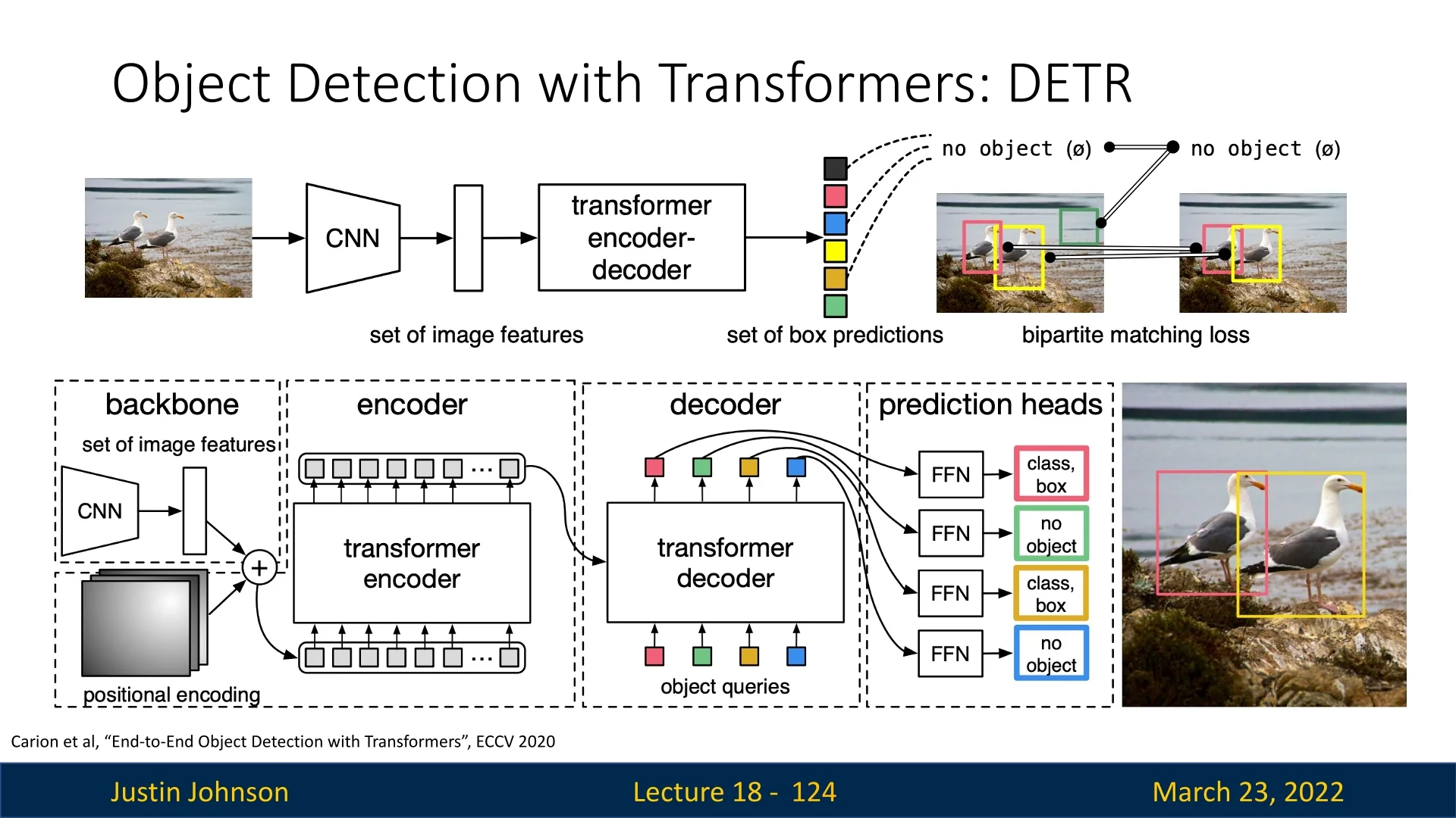
3. Learned Object Queries and Transformer Decoder
The decoder takes in \(N = 100\) learnable vectors called object queries, each intended to produce one detection result. These vectors are randomly initialized and updated during training to “ask” different questions about the image content.
- The encoder outputs serve as keys and values.
- The learned queries serve as queries in the decoder’s cross-attention layers.
This mirrors the original Transformer decoder from [664], adapted for detection instead of autoregressive text generation.
4. Interpreting Object Queries Each object query can be imagined as an attention-driven question, probing the image for different object types or regions.
For example, in the above figure 14.38, the colored boxes might be asking the following questions:
- “What small object is in the bottom-left?”
- “Is there something large in the center?”
Through training, each query vector specializes, covering distinct spatial areas, object sizes, or semantics. This is visualized in the following figure.
5. Why Attention is a Natural Fit Transformers are inherently suited for modeling pairwise relationships—making them a natural match for object detection, where understanding spatial interactions is key.
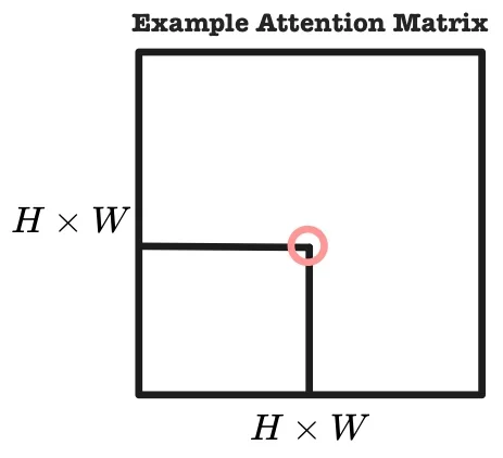
Hence, the encoder’s attention matrix (\(HW \times HW\)) can be viewed as modeling how each spatial location attends to others—implicitly capturing potential object extents. Though DeTR does not exploit this directly, it highlights how attention mechanisms align naturally with the structure of visual tasks, hinting at promising directions for future work in detection and region proposal learning.
Enrichment 14.8.4: DeTR Results, Impact, and Follow-Up Work
The introduction of DEtection TRansformer (DeTR) [64] marked a turning point in object detection by demonstrating that transformer-based architectures can achieve strong results without anchors or non-maximum suppression (NMS). DeTR generalizes remarkably well across:
- Objects of varying sizes: from small to large.
- Different object counts: from sparse to cluttered scenes.
- Challenging layouts: producing high-quality and coherent predictions.
DeTR’s learned object queries attend to semantically meaningful regions in the image. Some queries specialize in detecting small objects, others cover large or central regions, and many converge to interpretable modes that persist across datasets.
From Detection to Segmentation Thanks to its global attention mechanism and fixed set of learned queries, DeTR can be extended to perform panoptic segmentation. Instead of just bounding boxes, DeTR predicts a binary mask for each detected object in parallel. These masks are then merged using pixel-wise argmax, yielding instance segmentation results.
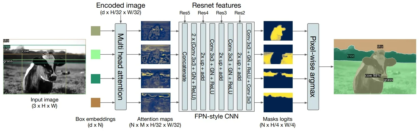
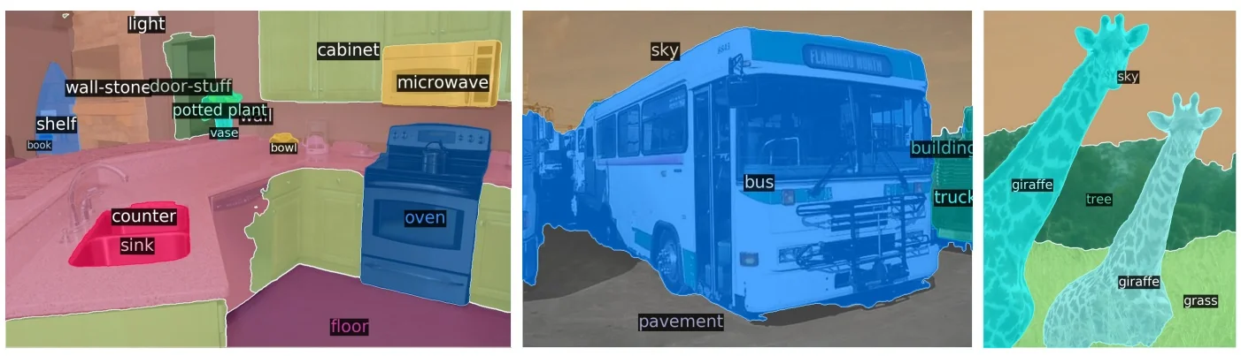
Real-World Usage: HuggingFace Implementation The practicality of DeTR has led to wide adoption in research and industry. For example, the HuggingFace Computer Vision Course provides a user-friendly notebook for fine-tuning DeTR on custom datasets, demonstrating its flexibility:
Follow-Up Works and Extensions Since its release, DeTR has inspired a rich line of research focused on addressing its main limitations—particularly training speed and convergence—while extending its capabilities:
- DAB-DeTR [382] was one of the first major improvements. It introduced dynamic anchor boxes by injecting learnable reference points into the object queries. This allowed the model to more effectively initialize and refine box predictions throughout training, leading to faster convergence and improved accuracy.
- DN-DeTR [338] further addressed the slow training issue by adding a denoising training objective. During training, noisy object queries are added and explicitly supervised, which stabilizes learning and accelerates convergence. This technique makes DeTR more competitive in terms of training time without sacrificing accuracy.
- DN-DETR [338] builds on both prior ideas and rethinks the decoder itself. It enables iterative refinement of predictions across decoder layers, where each stage progressively improves upon previous outputs. This dramatically speeds up convergence and reduces the computational footprint—bringing DeTR closer to real-time inference scenarios.
- Finally, NMS Strikes Back [478] challenges one of DeTR’s founding principles: the removal of non-maximum suppression. This work shows that reintroducing a lightweight form of NMS can help refine predictions and improve performance in crowded scenes—suggesting that hybrid approaches can sometimes outperform purist, end-to-end designs.
Broader Impact DeTR reshaped object detection by:
- Eliminating the need for hand-designed anchors and post-processing.
- Enabling a unified architecture for detection, segmentation, and panoptic tasks.
- Inspiring a new wave of research around set prediction in vision.
Its clean, end-to-end formulation led to more interpretable and modular designs, with applications extending beyond vision to robotics, remote sensing, and beyond.
Conclusion DeTR is a prime example of how Vision Transformers (ViTs) can be used to build practical, high-performance systems in computer vision. Despite being architecturally different from traditional CNNs, ViTs can now tackle nearly every major vision task—classification, detection, segmentation, and more.
The takeaway: Vision Transformers are an evolution—not a revolution. They offer a different lens through which we solve the same core problems. But with strong hardware alignment (favoring matrix multiplications over convolutions), ViTs often train and run faster than CNNs at comparable FLOPs. More importantly, they provide a seamless path toward multi-modal understanding, as seen in models like CLIP and Vision-Language Models (VLMs), empowering unified reasoning across image, text, and video.
Enrichment 14.9: Grounding DINO: DINO with Grounded Pre-Training
Enrichment 14.9.1: Motivation and Problem Setting
Motivation and Problem Setting
Classical object detectors such as Faster R-CNN or RetinaNet assume a closed-set label space: the model is trained and evaluated on a fixed, finite list of categories (e.g., the 80 COCO classes). This assumption is incompatible with many real applications, where users wish to detect arbitrary concepts specified at test time by free-form text prompts (e.g., “person holding a red ball”, “traffic light with a red arrow”). In this regime, models must understand language and localize novel categories without box-level supervision for every possible concept.
Grounding DINO [384] addresses this problem by “marrying” a strong DETR-style detector (DINO-DETR [337]) with grounded pre-training on large-scale image–text data. The model is designed to:
- Support closed-set detection on standard datasets such as COCO by fine-tuning on box-annotated data.
- Enable open-set detection by conditioning on prompts containing arbitrary category names or phrases.
- Handle referring expression comprehension (REC), where the input is a single phrase (e.g., “the man in a red shirt”) and the goal is to localize exactly the described instance.
The following figure (reproduced from [384]) highlights the conceptual difference between closed-set detection and open-set phrase grounding, and illustrates an image-editing application obtained by coupling Grounding DINO with Stable Diffusion [548].
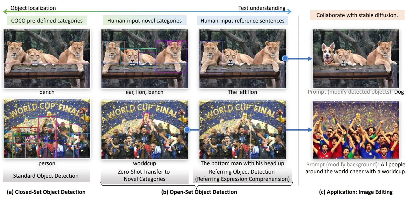
Grounding DINO: Multi-Level Language Fusion
Grounding DINO transforms the closed-set detector DINO-DETR into an open-vocabulary learner by injecting language supervision at three tightly coupled stages of the architecture [384]. Rather than processing the image in isolation and classifying boxes against a fixed vocabulary, Grounding DINO treats detection as a progressive alignment between visual features and a text prompt (e.g., “furry animal on grass”). The same BERT-extracted text embeddings are threaded through the feature enhancer (encoder), the language-guided query initialization, and the cross-modality decoder, so that all components operate in a shared vision–language space.
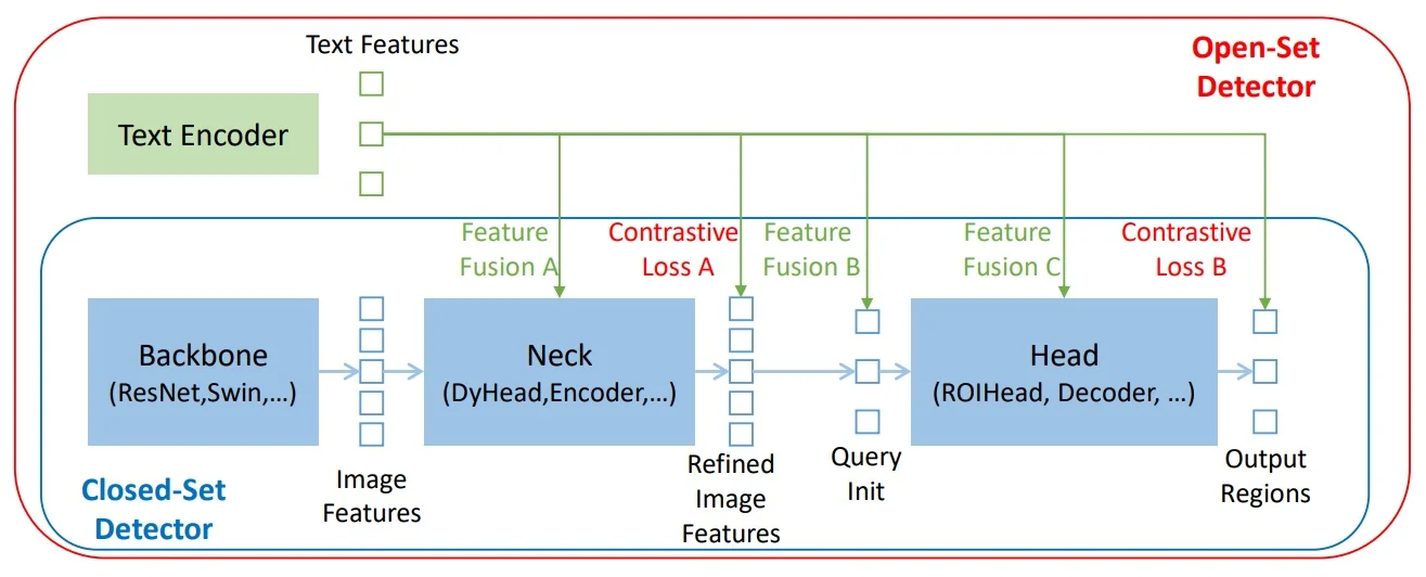
Enrichment 14.9.2: Method
Core idea and progressive fusion philosophy Grounding DINO [384] upgrades the strong closed-set detector DINO-DETR [337] into an open-vocabulary detector by replacing fixed classifier weights with region-to-phrase matching in a shared embedding space. Instead of predicting logits over a pre-defined label set, each region representation is compared (via dot products) to text-token embeddings produced by a BERT encoder. The same text features are woven into the network at three points so that early image–text alignment directly supports query initialization and final decoding. Architecturally, Grounding DINO combines a DETR-style set-prediction detector equipped with multi-scale deformable attention (from Deformable DETR/DINO-DETR [827, 337]) with GLIP-style grounded pre-training on large detection + caption corpora [349], but with much stronger cross-modal fusion in both encoder and decoder.
It is helpful to view the architecture as a three-phase refinement cascade on top of a dual encoder. These phases are conceptual stages within a single end-to-end forward pass: they are not trained separately. In every training step, the model runs through Phases A, B, and C once, and losses from the encoder and decoder are backpropagated jointly.
- Phase A: Feature Enhancer encoder. A bi-directional image–text fusion encoder with deformable attention and dense encoder-level grounding (Contrastive Loss A). It produces grounded image and text tokens, encoder-level box predictions, and a dense region–to–token similarity map, whose rows are anchored to spatial image locations and whose columns correspond to text tokens. Although the image features are repeatedly updated by self- and cross-attention, these layers only change the contents of the token vectors: they never reorder the sequence or modify each token’s associated positional/reference coordinates. The \(i\)-th output token therefore still corresponds to the same backbone cell (position \(\mathbf {p}_i\), scale \(s_i\)) as the \(i\)-th input token. This preserved spatial correspondence allows Phase B to interpret each row of \(\tilde {X}_I \tilde {X}_T^\top \) as a spatial heatmap over the prompt and to convert high-scoring image tokens, together with their encoder-predicted boxes, into dynamic decoder anchors.
- Phase B: Language-guided query selection. A deterministic module that uses the Phase-A similarity map and encoder box predictions to seed decoder queries at text-relevant locations with dynamic anchors.
- Phase C: Cross-modality decoder. A DINO-DETR-style decoder enriched with text cross-attention and decoder-level grounding (Contrastive Loss B). It refines this query set into final region–phrase predictions.
Each phase refines the previous one: Phase A aligns dense tokens and learns encoder-level box predictions; Phase B converts the strongest region–text matches into sparse queries with dynamic anchors; Phase C iteratively refines these queries using image and text, producing final boxes and open-vocabulary scores. Importantly, bounding boxes are predicted in both Phase A and Phase C: the encoder boxes (of Phase A) provide deep supervision and good anchors, while the decoder boxes (of Phase C) are the final outputs.
Phase A: Feature Enhancer and encoder-level grounding Phase A operates on top of two unimodal encoders and gradually pulls their tokens into a shared vision–language space. Crucially, all subsequent attention and feed-forward blocks act on the features of each token while preserving the token ordering and its associated positional information: a token that originated from backbone cell \((x_i,y_i)\) on level \(s_i\) remains the \(i\)-th image token throughout the Feature Enhancer. Attention may aggregate information from many locations and from text, but it never changes which spatial cell a given token index refers to. At the end of Phase A we therefore still have:
- Grounded image tokens whose indices and positional encodings anchor them to specific receptive-field regions in the image.
- Grounded text tokens tied to individual words or sub-words in the prompt.
- Encoder-level box predictions attached to each image token.
- A dense similarity matrix \(M = \tilde {X}_I \tilde {X}_T^\top \) that can be read as a region–to–token map, because rows correspond to spatially anchored image tokens and columns to text tokens.
Phase B will compress this dense similarity information into a sparse set of text-guided queries, and all of this is trained jointly via Contrastive Loss A.
Inputs and notation (dual encoder).
- Image backbone (Swin Transformer). A Swin Transformer [395], pre-trained on large-scale classification and optionally further tuned in a DINO-DETR detector [337], produces multi-scale feature maps \[ X_I^{(s)} \in \mathbb {R}^{H_s \times W_s \times d_{\mbox{img}}}, \quad s \in \{1,\dots ,S\}. \] Each map is projected by a \(1\times 1\) convolution to a shared hidden dimension \(d = 256\) and flattened to a sequence \[ X_I^{(s)} \in \mathbb {R}^{N_s \times d}, \quad N_s = H_s W_s. \] Concatenating all scales yields the image token sequence \[ X_I \in \mathbb {R}^{N_I \times d}, \quad N_I = \sum _{s=1}^{S} N_s, \] where each row is tied to a specific spatial location and stride in the feature pyramid.
- Text backbone (BERT with sub-sentence prompts). The text branch uses a BERT-base encoder [121]. The prompt \(T\) is a single string of phrases separated by delimiters (e.g., “cat . baseball glove . fire hydrant .”), a format that will later support sub-sentence masking. After tokenization and BERT encoding, a linear projection maps BERT’s hidden states into the same dimension \(d\): \[ X_T \in \mathbb {R}^{N_T \times d}, \quad N_T \leq 256. \]
At this stage, \(X_I \in \mathbb {R}^{N_I \times d}\) and \(X_T \in \mathbb {R}^{N_T \times d}\) share dimension \(d\), but originate from disjoint pre-training regimes (vision vs. language). The Swin backbone has never seen text; BERT has never seen images. Phase A is responsible for pulling these two streams into a shared, grounded space.
Multi-scale deformable attention (MSDeformAttn).
Before describing the Feature Enhancer sub-blocks, it is helpful to recall the multi-scale deformable attention module reused from Deformable DETR [827] and DINO-DETR [337]. It appears both in the encoder (Phase A) and in the decoder (Phase C).
Suppose the backbone outputs \(S\) feature levels: \[ X_I^{(s)} \in \mathbb {R}^{H_s \times W_s \times d}, \quad N_s = H_s W_s, \quad N_I = \sum _{s=1}^{S} N_s. \] Each token corresponds to a scale \(s\) and a coordinate \(\mathbf {p} = (x,y)\) with normalized reference point \(\mathbf {r}_i^{(s)} \in [0,1]^2\).
Dense self-attention baseline.
Standard self-attention over all image tokens would compute, for queries \(Q\), keys \(K\), and values \(V\), \[ \mathrm {SA}(i) = \sum _{j=1}^{N_I} \alpha _{ij} V_j, \quad \alpha _{ij} = \mbox{softmax}_j\left (\frac {Q_i K_j^\top }{\sqrt {d_k}}\right ), \] with \(O(N_I^2)\) complexity and no explicit use of the multi-scale structure beyond positional encodings.
Multi-scale deformable attention.
Deformable attention replaces dense summation with sparse, geometry-aware sampling. For each query token \(i\), head \(h\), scale \(s\), and sampling index \(k \in \{1,\dots ,K\}\), the module predicts:
- Offsets \(\Delta \mathbf {p}_i^{(h,s,k)} \in \mathbb {R}^2\).
- Unnormalized weights \(A_i^{(h,s,k)} \in \mathbb {R}\).
Sampling locations in normalized coordinates are \[ \mathbf {p}_i^{(h,s,k)} = \mathbf {r}_i^{(s)} + \Delta \mathbf {p}_i^{(h,s,k)}. \] Feature values are obtained via bilinear interpolation on scale-\(s\) feature maps: \[ \mathbf {v}_i^{(h,s,k)} = \mbox{BilinearSample}\bigl (X_I^{(s)}, \mathbf {p}_i^{(h,s,k)}\bigr ) \in \mathbb {R}^{d/H}. \] After normalizing \(A_i^{(h,s,k)}\) over all \((s,k)\) for each head to obtain \(\tilde {A}_i^{(h,s,k)}\), deformable attention produces: \[ \mathrm {MSDeformAttn}(i) = \sum _{h=1}^{H} W_h^{\mathrm {out}} \left ( \sum _{s=1}^{S} \sum _{k=1}^{K} \tilde {A}_i^{(h,s,k)}\, \mathbf {v}_i^{(h,s,k)} \right ), \] where \(W_h^{\mathrm {out}}\) are per-head output projections. Complexity is \(O(N_I H S K)\), linear in the number of tokens.
In the Feature Enhancer (Phase A), this operation refines each image token before any image–text cross-attention. A token at stride 16 near a cat’s ear, for example, can sample:
- Finer details from stride-8 features (fur texture, edge details).
- Similar-scale neighbors from stride-16 features (shape continuity).
- Coarser context from stride-32 features (overall body and background).
In the decoder (Phase C), the same module is used as cross-attention from queries to image features. Each query \(q_k^{(l)}\) has a current anchor box \((c_x,c_y,w,h)\), which is converted into one or several reference points across scales. For each head and scale, the module predicts offsets and weights, samples a few positions near the anchor, and aggregates them as above. This lets each query:
- Look locally around its current box guess across all scales.
- Refine its internal representation with multi-scale evidence.
- Prepare for text fusion by providing a geometry-aware visual summary to the subsequent text cross-attention.
This MSDeformAttn block is therefore the main mechanism by which Grounding DINO inherits the efficiency and multi-scale robustness of Deformable DETR/DINO-DETR [827, 337].
After defining MSDeformAttn, we can now describe the four sub-blocks of each Feature Enhancer layer. At layer \(\ell \), we keep image tokens \(X_I^{(\ell )} \in \mathbb {R}^{N_I \times d}\) and text tokens \(X_T^{(\ell )} \in \mathbb {R}^{N_T \times d}\); each layer applies:
- 1.
- Deformable self-attention on image tokens using MSDeformAttn.
- 2.
- Masked self-attention on text tokens.
- 3.
- Image-to-text cross-attention.
- 4.
- Text-to-image cross-attention, followed by modality-specific FFNs.
We describe these in turn.
(A1) Deformable self-attention on image tokens.
Using the MSDeformAttn module described above, the image stream is refined as \[ \hat {X}_I^{(\ell )} = \mbox{MSDeformSelfAttn}\bigl (X_I^{(\ell )}\bigr ), \quad \hat {X}_I^{(\ell )} \in \mathbb {R}^{N_I \times d}. \]
Here \(X_I^{(\ell )}\) is the concatenation of all backbone scales; each token has an associated reference point across the multi-scale pyramid, and MSDeformSelfAttn aggregates a small, learned set of samples around that point across all levels. Conceptually, each patch token becomes a compact, geometry-aware summary of its local multi-scale neighborhood, rather than a raw backbone descriptor, which stabilizes the subsequent cross-modal alignment.
(A2) Text self-attention with sub-sentence mask.
Text tokens are refined by masked self-attention: \[ \hat {X}_T^{(\ell )} = \mbox{SelfAttn}\bigl (X_T^{(\ell )}, \mbox{mask}_{\mbox{sub-sent}}\bigr ), \quad \hat {X}_T^{(\ell )} \in \mathbb {R}^{N_T \times d}. \] In open-vocabulary detection, the prompt is typically a concatenation of many category phrases and referring expressions. Naive word-level attention would let “cat” attend to “baseball glove”, mixing unrelated semantics. Grounding DINO avoids this by constructing a sub-sentence mask from simple punctuation conventions:
- Prompt formatting. The prompt is written as a single string where phrases are separated by delimiters (e.g., “.”).
- Segment assignment. After tokenization, each token is assigned a segment id according to which phrase it belongs to.
- Masked attention. The attention mask \(\mbox{mask}_{\mbox{sub-sent}}\) permits attention only within the same segment; cross-phrase entries are set to zero, yielding a block-diagonal pattern.
For example, for \[ \texttt{"a small brown dog . red car . person wearing a blue hat ."}, \] we obtain segments such as:
- Segment 0. Tokens of “a small brown dog”.
- Segment 1. Tokens of “red car”.
- Segment 2. Tokens of “person wearing a blue hat”.
Tokens inside each phrase still see all of their local context (adjectives, prepositions, compound nouns), while phrases remain cleanly separated as independent detection targets. This sub-sentence representation is exactly the option found empirically best in the Grounding DINO paper [384], and it is reused wherever text self-attention appears.
Sub-sentence text representation The paper compares three ways of encoding prompts [384]:
- Sentence-level. Each phrase is encoded in a separate BERT pass and pooled; this preserves intra-phrase structure but is inefficient and discards token-level detail.
- Word-level. All phrases are concatenated and encoded jointly with full self-attention; this is efficient but allows spurious cross-phrase interactions.
- Sub-sentence-level. All phrases are encoded jointly, but self-attention is masked to stay within each phrase, as in (A2). This keeps intra-phrase context, prevents cross-phrase contamination, and amortizes BERT computation.
This representation is used consistently in both Phase A and Phase C whenever text attention appears.
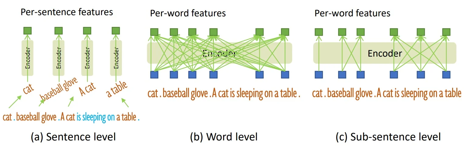
(A3) Image-to-text cross-attention (\(I \rightarrow T\)): text tokens collect visual evidence.
Once the unimodal streams have been strengthened, Phase A begins cross-modal fusion. First, text tokens query the image tokens: \[ \tilde {X}_T^{(\ell )} = \mbox{CrossAttn}_{I \rightarrow T}\bigl (Q = \hat {X}_T^{(\ell )},\, K = \hat {X}_I^{(\ell )},\, V = \hat {X}_I^{(\ell )}\bigr ), \quad \tilde {X}_T^{(\ell )} \in \mathbb {R}^{N_T \times d}. \] In matrix shapes: \begin {align*} Q_T^{(\ell )} &= W_q \hat {X}_T^{(\ell )} \in \mathbb {R}^{N_T \times d_q},\\ K_I^{(\ell )} &= W_k \hat {X}_I^{(\ell )} \in \mathbb {R}^{N_I \times d_k},\\ V_I^{(\ell )} &= W_v \hat {X}_I^{(\ell )} \in \mathbb {R}^{N_I \times d_v}, \end {align*}
with learned projections \(W_q, W_k, W_v\). The attention matrix is \[ A_{T \leftarrow I}^{(\ell )} = \mbox{softmax}\!\left (\frac {Q_T^{(\ell )} K_I^{(\ell )\top }}{\sqrt {d_q}}\right ) \in \mathbb {R}^{N_T \times N_I}, \] where each row gives weights from one text token to all image tokens. The cross-attended update is \[ \hat {U}_T^{(\ell )} = A_{T \leftarrow I}^{(\ell )} V_I^{(\ell )} \in \mathbb {R}^{N_T \times d_v}. \] With a residual path back to dimension \(d\), the new text tokens are \[ \tilde {X}_T^{(\ell )} = \hat {X}_T^{(\ell )} + \hat {U}_T^{(\ell )}. \] Each row of \(\tilde {X}_T^{(\ell )}\) is thus a mixture of:
- A linguistic component coming from the original BERT embedding \(\hat {X}_T^{(\ell )}\).
- A visual component given by a weighted sum of image tokens \(V_I^{(\ell )}\).
For the token encoding “cat”, the corresponding row of \(A_{T \leftarrow I}^{(\ell )}\) peaks on image locations that look like cats (fur, face, whiskers), so the visual component aggregates those regions. The residual connection keeps the text token anchored in language space while adding an image-dependent correction that reflects how this particular image instantiates “cat”. Shape-wise, the number of text tokens remains \(N_T\); only their contents change.
(A4) Text-to-image cross-attention (\(T \rightarrow I\)): image tokens pull semantics from text.
Next, information flows in the opposite direction: image tokens query the now image-conditioned text tokens: \[ \tilde {X}_I^{(\ell )} = \mbox{CrossAttn}_{T \rightarrow I}\bigl (Q = \hat {X}_I^{(\ell )},\, K = \tilde {X}_T^{(\ell )},\, V = \tilde {X}_T^{(\ell )}\bigr ), \quad \tilde {X}_I^{(\ell )} \in \mathbb {R}^{N_I \times d}. \] In matrix form, \begin {align*} Q_I^{(\ell )} &= W'_q \hat {X}_I^{(\ell )} \in \mathbb {R}^{N_I \times d_q},\\ K_T^{(\ell )} &= W'_k \tilde {X}_T^{(\ell )} \in \mathbb {R}^{N_T \times d_k},\\ V_T^{(\ell )} &= W'_v \tilde {X}_T^{(\ell )} \in \mathbb {R}^{N_T \times d_v}, \end {align*}
and \[ A_{I \leftarrow T}^{(\ell )} = \mbox{softmax}\!\left (\frac {Q_I^{(\ell )} K_T^{(\ell )\top }}{\sqrt {d_q}}\right ) \in \mathbb {R}^{N_I \times N_T}, \qquad \hat {V}_I^{(\ell )} = A_{I \leftarrow T}^{(\ell )} V_T^{(\ell )} \in \mathbb {R}^{N_I \times d_v}. \] With a residual path, \[ \tilde {X}_I^{(\ell )} = \hat {X}_I^{(\ell )} + \hat {V}_I^{(\ell )}. \]
Each row of \(\tilde {X}_I^{(\ell )}\) therefore becomes a mixture of:
- A visual component inherited from the backbone and deformable self-attention.
- A semantic component given by a weighted sum of text tokens that best explain that region.
For a patch on the cat’s ear, the corresponding row of \(A_{I \leftarrow T}^{(\ell )}\) has high weight on the tokens of the “cat” phrase (and possibly modifiers such as “small” or “brown”) and low weight on unrelated phrases such as “fire hydrant”. The updated feature becomes a visually grounded but text-aligned representation of that patch. Importantly, while the feature vector mixes information from many locations and tokens, the index of each image token (and its reference point in the pyramid) still tells us from which patch of the input it originated; attention moves information, not coordinates. The image token grid and multi-scale structure remain intact; only the feature vectors are rotated in the joint space.
(A5) FFNs, progressive alignment, and Contrastive Loss A.
After the two cross-attention directions, modality-specific FFNs with residual connections are applied: \[ X_I^{(\ell +1)} = \mbox{FFN}_I\bigl (\tilde {X}_I^{(\ell )}\bigr ), \quad X_T^{(\ell +1)} = \mbox{FFN}_T\bigl (\tilde {X}_T^{(\ell )}\bigr ). \] Stacking \(L_{\mbox{enh}}\) layers yields a sequence of transformations \[ (X_I^{(0)}, X_T^{(0)}) \rightarrow (X_I^{(1)}, X_T^{(1)}) \rightarrow \dots \rightarrow (X_I^{(L_{\mbox{enh}})}, X_T^{(L_{\mbox{enh}})}), \]
where at each level:
- Text tokens evolve from generic BERT embeddings into mixtures of linguistic content and the image regions that instantiate each phrase in the current image.
- Image tokens evolve from purely visual patches into mixtures of visual content and the phrase embeddings that best describe them.
Because both branches live in \(\mathbb {R}^{d}\), we can form the similarity matrix \[ M = \tilde {X}_I \tilde {X}_T^\top \in \mathbb {R}^{N_I \times N_T}, \] which is precisely the dense region–to–token similarity map mentioned above, now written explicitly as an image-token–to–text-token affinity matrix. Concretely:
- Row \(i\) of \(\tilde {X}_I\) is the embedding \(z_i^\top \in \mathbb {R}^{1 \times d}\) of the \(i\)-th image token, which originated from a specific backbone cell (a patch at location \((x_i,y_i)\) on some feature level) and now encodes a context-enriched representation of that patch.
- Row \(j\) of \(\tilde {X}_T\) is the embedding \(t_j^\top \in \mathbb {R}^{1 \times d}\) of the \(j\)-th text token, anchored to a particular word or sub-word (e.g., “cat”, “glove”, “blue”) within its phrase.
The entry \[ M_{ij} = z_i^\top t_j \] is therefore the compatibility between the patch-level token at spatial location \(i\) and the word-level token \(j\). Each row of \(M\) is a score vector over all words for a single spatial token, and each column is a score vector over all spatial tokens for a single word. It is thus natural to interpret \(M\) as a dense region–to–token affinity map, which Phase B will reuse for language-guided query selection.
To drive this alignment, Grounding DINO attaches detection heads directly to the encoder outputs and applies Contrastive Loss A [384, 349]. Each image token \(z_i\) (row of \(\tilde {X}_I\)) is treated as a candidate region:
- Box regression (encoder-level boxes). For each image token \(z_i\), which is tied to a particular backbone cell with center \((x_i,y_i)\) and stride \(s_i\), a small MLP predicts a 4D box vector \[ \hat {b}_i = (\hat {c}_x,\hat {c}_y,\hat {w},\hat {h}) \] in normalized image coordinates. Conceptually, the head starts from a default box centered at the token’s patch center \((x_i,y_i)\) with a size proportional to the feature-map stride \(s_i\), and learns offsets and scale changes around this default (mirroring the reference-point box parameterization used in Deformable DETR and DINO-DETR [827, 337]). Hungarian matching is then applied between the set of encoder-level predictions \(\{\hat {b}_i\}\) and ground-truth boxes, with a cost that combines classification (from the contrastive scores) and geometry (L1 and GIoU) as in DETR-style detectors [64]; matched tokens are trained with L1 and GIoU losses. These encoder-level boxes are not the final outputs: they (1) provide deep supervision that teaches each encoder token to propose a box anchored at its own patch, and (2) supply the dynamic anchors that Phase B will reuse when initializing decoder queries.
-
Contrastive classification (Contrastive Loss A). Instead of a fixed classifier matrix, classification is performed by comparing \(z_i\) to all text tokens \(t_j\) (rows of \(\tilde {X}_T\)): \[ u_{ij} = z_i^\top t_j,\qquad j = 1,\dots ,N_T. \]
For a token \(z_i\) matched (via Hungarian) to a ground-truth box annotated with a phrase, a small subset of text tokens (those belonging to that phrase) are labeled as positives; all other tokens are negatives. This yields a highly imbalanced multi-label problem: per image token, the vast majority of word tokens are negatives, just as most anchors in dense detectors are background. Grounding DINO therefore uses a focal-style multi-label contrastive loss (inspired by GLIP [349]), which down-weights easy negatives and focuses learning on hard negatives and the few positive token matches. In effect, this applies a CLIP-style contrastive objective at dense spatial locations, while addressing the severe foreground–background imbalance that arises in detection.
Gradients from Contrastive Loss A propagate through all Feature Enhancer layers, training the network to use its cross-attention blocks so that corresponding region and phrase features become similar and unrelated pairs become dissimilar. To summarize, by the end of Phase A, \(\tilde {X}_I\) and \(\tilde {X}_T\) form a well-aligned pair of token sets, \(M = \tilde {X}_I \tilde {X}_T^\top \) behaves as a high-quality region–to–word affinity map, and each image token carries an encoder-level box prediction \(\hat {b}_i\) that will be exploited in Phase B.
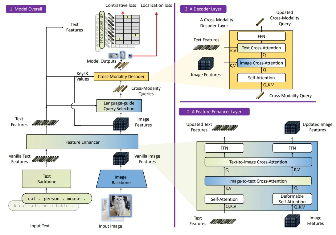
Phase B: Language-guided query selection Phase B takes the dense, grounded encoder tokens from Phase A and converts them into a sparse set of decoder queries that are already biased toward text-relevant regions. Crucially, Phase B is a loss-free, deterministic transformation executed inside the same forward pass: it does not introduce new parameters or a separate training stage. Instead, it harvests the information created by Contrastive Loss A—both the affinity matrix \(M = \tilde {X}_I \tilde {X}_T^\top \) and the encoder-level box predictions \(\hat {b}_i\)—to build a strong “warm start” for the decoder.
After Phase A we have \(\tilde {X}_I \in \mathbb {R}^{N_I \times d}\) and \(\tilde {X}_T \in \mathbb {R}^{N_T \times d}\). Each image token \(\tilde {X}_I[i,:]\) is still associated with a particular spatial cell in the backbone pyramid: it originated from a specific feature map level \(s_i\) and grid location \((x_i,y_i)\) (a patch of the input image), inherited that position’s reference point for deformable attention, and now carries an encoder-level box prediction \(\hat {b}_i\) anchored around that patch. Cross-attention has mixed information between patches and phrases, but the token indices and positional encodings retain the link “token \(i\) \(\leftrightarrow \) receptive-field region centered at \((x_i,y_i)\)”.
(B1) Scoring encoder tokens by text similarity.
Using the grounded features, Grounding DINO reuses the similarity matrix \begin {equation} S = \tilde {X}_I \tilde {X}_T^\top \in \mathbb {R}^{N_I \times N_T}, \end {equation}
where \(S_{ij}\) measures how similar image token \(i\) is to text token \(j\). To obtain a single relevance score per image token, \begin {equation} s_i = \max _j S_{ij}, \quad i = 1,\dots ,N_I. \end {equation} This asks, for each spatial token: Does this look strongly like any word or phrase in the prompt? The max pools over all words and avoids rewarding locations that weakly match many unrelated words.
The indices of the top \(N_q\) tokens under this score, \begin {equation} \mathcal {I}_{N_q} = \mathrm {Top}_{N_q}\bigl (s_1,\dots ,s_{N_I}\bigr ), \quad N_q \approx 900 \mbox{ in the reference configurations}, \end {equation} are taken as language-guided encoder locations [384]. These are precisely the tokens that Phase A and Contrastive Loss A have already made strongly aligned with some phrase.
(B2) From encoder tokens to dynamic anchor boxes.
Each index \(i \in \mathcal {I}_{N_q}\) corresponds to:
- A spatial position \((x_i, y_i)\) and stride \(s_i\) in the feature pyramid (the patch from which the token originated).
- An encoder-level box prediction \(\hat {b}_i = (\hat {c}_x,\hat {c}_y,\hat {w},\hat {h})\) in normalized image coordinates, produced in Phase A by the encoder head.
Following DAB-DETR and DINO-DETR [382, 337], Grounding DINO uses these encoder-level predictions directly as dynamic anchor boxes for decoder queries:
- Anchor centers. The initial anchor center \((c_x,c_y)\) of the query is set equal to the predicted center \((\hat {c}_x,\hat {c}_y)\).
- Anchor sizes. The initial anchor size \((w,h)\) is set equal to \((\hat {w},\hat {h})\), adapting to small objects at fine scales and large objects at coarse scales.
There is no separate box regression in Phase B: Phase B simply copies the encoder’s prediction \(\hat {b}_i\) into the query’s anchor parameterization.
The tuple \[ (c_x,c_y,w,h) := \hat {b}_i \] is then embedded (via the same sinusoidal box encoding + learned projections used in DAB-DETR/DINO-DETR) into a positional query vector. Because these anchors come from data-dependent encoder predictions instead of a fixed grid, they adapt to each image’s object sizes and locations. Conceptually, Phase A has already told us where each phrase is likely to appear; Phase B turns those encoder boxes into starting points for the decoder. The subsequent refinement of these anchors into final boxes happens in Phase C, not in Phase B.
(B3) Content embeddings and mixed query selection
As in DAB-DETR/DINO-DETR [382, 337], each decoder query is factored into:
- A positional part given by an (embedded) anchor box \((c_x,c_y,w,h)\).
- A content part given by a learnable embedding in \(\mathbb {R}^d\), independent of spatial location.
Concretely, the model maintains a bank of content embeddings \[ E_{\mbox{content}} \in \mathbb {R}^{N_q \times d}, \] which is a parameter matrix learned over the whole training set. For a single image, these \(N_q\) rows become the content part of that image’s queries. For a mini-batch of size \(B\), the same bank is tiled across the batch, yielding a tensor of shape \(\mathbb {R}^{B \times N_q \times d}\). In this sense, the content embeddings are “shared across images”: the same \(N_q\) learnable query vectors are reused for every image, but their positional part (the anchor boxes) is image-dependent.
Grounding DINO adopts DINO-DETR’s mixed query strategy, in which the same content bank \(E_{\mbox{content}}\) is combined with anchors coming from three different sources:
-
Purely learned queries. A subset of queries uses anchors that are also learned parameters, not tied to any encoder token or text. Intuitively, these queries act as generic “questions” that the decoder asks about every image, such as:
- “Is there any large object roughly in the center of the image?”.
- “Is there a small, elongated object near the top edge?”.
- “Is there a blob-like region with strong contrast anywhere?”.
Because both their content and positional parts are image-agnostic, they can learn reusable priors about common object layouts and backgrounds. They also ensure that, even if the language signal is weak or noisy, the decoder still has some DINO-like, text-free queries probing the scene.
-
Objectness-guided queries (DINO-style). Following DINO-DETR [337], a second subset of queries uses anchors taken from encoder tokens that look object-like, according to a generic objectness score from the encoder-level detection head (language-agnostic foreground likelihood, as in DINO). These anchors inherit:
- Centers and sizes from the encoder’s box predictions at those tokens.
- No direct dependence on the prompt text in their selection.
Conceptually, these queries play the role of “proposal-like” queries: they start on regions the encoder suspects to contain some object, regardless of which phrase is being asked. Grounding DINO keeps a small number of such DINO-style queries mainly for stability and backward compatibility with the strong closed-set detector it builds upon.
- Language-guided queries. Finally, a large subset of queries uses anchors derived from the language-guided indices \(\mathcal {I}_{N_q}\) in (B1)–(B2). For each selected encoder token \(i \in \mathcal {I}_{N_q}\), we take its encoder-level prediction \[ \hat {b}_i = (\hat {c}_x,\hat {c}_y,\hat {w},\hat {h}) \] and set the query’s anchor to \((c_x,c_y,w,h) = \hat {b}_i\). These anchors are then embedded (via sinusoidal encodings and learned projections) and combined with rows of \(E_{\mbox{content}}\) to form the initial query set. Because the indices were chosen by high image–text similarity, these queries start exactly on regions that Phase A has already aligned strongly with some phrase in the prompt.
In the reference configurations, language-guided queries occupy the majority of the query budget (hundreds out of the total \(N_q = 900\) queries), while the remaining queries are split between purely learned and DINO-style objectness-guided anchors. The exact numerical split is a hyperparameter rather than a core design point; what matters is that:
- Language-guided queries dominate, tightly coupling many queries to the prompt.
- Purely learned queries provide text-agnostic priors and a safety net when text supervision is weak or missing.
- Objectness-guided queries retain a small pool of DINO-like, proposal-style anchors focused on visually salient regions, independent of the textual phrasing.
In all cases, the content embeddings are shared across images, but the anchors (and thus the positional encodings) are recomputed per image, so each image still has its own \(N_q\) queries.
Formally, the language-guided part of the selection can be summarized as:
def language_guided_query_selection(X_I, X_T, num_queries):
    # X_I: [N_I, d] grounded image features (Phase A outputs)
    # X_T: [N_T, d] grounded text features

    # 1. Compute image{text similarity
S = X_I @ X_T.T              # [N_I, N_T]

# 2. Collapse over text to get one relevance score per image token
s = S.max(dim=1).values      # [N_I]

# 3. Take top-k indices as language-guided encoder locations
indices = s.topk(num_queries).indices  # [num_queries]
return indices
Intuition: Phase B as a warm start.
In DINO-DETR, encoder-based queries are chosen using generic objectness scores, so the decoder must discover both where objects are and what they are [337]. Grounding DINO retains this idea but adds a strong language-guided path. Phase A + Contrastive Loss A make tokens overlapping, say, a “cat” box highly similar to the “cat” text tokens; Phase B then:
- Keeps some purely learned and objectness-guided queries to probe object-like regions in a prompt-agnostic way.
- Adds many more queries whose anchors are copied directly from the highest-scoring image tokens under the prompt, i.e., tokens that already look like some phrase in the text.
The decoder in Phase C therefore starts from a rich mixture of queries: some asking general, text-free questions about the scene, and many already centered on plausible objects that Phase A believes correspond to the current prompt. This dramatically shrinks the decoder’s search space and makes it much easier to converge to accurate, text-grounded detections.
Phase C: Cross-modality decoder and Contrastive Loss B Phase C takes the full query set constructed in Phase B—dominated by, but not limited to, language-guided queries—and refines it into final region–phrase predictions by repeatedly attending to image features (for geometry and appearance) and text tokens (for semantics). As with Phase A, this decoder is trained jointly in a single end-to-end optimization: Contrastive Loss B is applied on top of its outputs at each training step.
Phase C uses a DINO-DETR-style decoder with an additional text cross-attention block. It takes as input:
- Initial queries \(Q^{(0)} \in \mathbb {R}^{N_q \times d}\) with content and anchor components (some purely learned, some objectness-guided, many language-guided).
- Grounded image features \(\tilde {X}_I \in \mathbb {R}^{N_I \times d}\) from Phase A.
- Grounded text features \(\tilde {X}_T \in \mathbb {R}^{N_T \times d}\) from Phase A.
At decoder layer \(l\), four sub-blocks are applied:
- 1.
- Query self-attention. \[ \hat {Q}^{(l)} = \mbox{SelfAttn}\bigl (Q^{(l)}\bigr ), \] enabling queries to communicate, share information, and suppress duplicates (e.g., two queries that see the same object can negotiate which one will take responsibility).
- 2.
- Image deformable cross-attention (reuse of MSDeformAttn). \[ \tilde {Q}^{(l)} = \mbox{MSDeformCrossAttn}\bigl (\hat {Q}^{(l)}, \tilde {X}_I\bigr ), \] where each query, using its current anchor as reference, applies the same MSDeformAttn mechanism as in Phase A, but now as cross-attention from queries to image tokens. This lets each query sample a small set of positions around its anchor across all image scales, refining its geometric and appearance representation while keeping complexity linear.
- 3.
- Text cross-attention (new relative to DINO-DETR). \[ \bar {Q}^{(l)} = \mbox{CrossAttn}_{\mbox{text}}\bigl (\tilde {Q}^{(l)}, \tilde {X}_T\bigr ), \] allowing each query to aggregate information from text tokens and decide which phrases best explain its current visual evidence. Conceptually, the query “asks” the prompt: given what I see around my anchor, am I a “red car”, a “person in blue hat”, or background?
- 4.
- Feed-forward network. \[ Q^{(l+1)} = \mbox{FFN}\bigl (\bar {Q}^{(l)}\bigr ). \]
After \(L_{\mbox{dec}} = 6\) layers, each query \(q_i = Q^{(L_{\mbox{dec}})}_i\) encodes a candidate object with refined geometry, visual features, and text alignment.
Decoder-level supervision (Contrastive Loss B).
The final queries are supervised similarly to DINO-DETR but with open-vocabulary classification [337, 384]:
- Box regression (decoder boxes). Hungarian matching assigns each ground-truth region–phrase pair to at most one query, and matched queries predict boxes trained with L1 and GIoU losses. These decoder-level predictions, not the encoder boxes, are the final outputs used at inference time; they refine the initial anchors copied from Phase A.
- Region-to-phrase contrastive classification (Contrastive Loss B). For each matched query \(q_i\) and text token \(t_j\), logits \[ \hat {u}_{ij} = q_i^\top t_j \] are computed and trained with a focal-like contrastive loss [384]. As in Phase A, each positive query is associated with a small subset of positive text tokens (those belonging to its ground-truth phrase), while all remaining tokens are negatives. The imbalance is even more severe here: most queries are background (or redundant) and most text tokens are irrelevant for any given query. Using a focal term again down-weights the many easy negatives (queries that clearly do not match a phrase, or phrases that clearly do not match a query) and forces the model to concentrate on hard negatives and the few positive region–token pairs.
The overall training objective combines encoder- and decoder-level terms (plus standard DETR-style auxiliary losses on intermediate decoder layers). Conceptually, \[ \mathcal {L} = \lambda _{\mbox{A}}\, \mathcal {L}_{\mbox{enc}}^{\mbox{box+contr}} + \lambda _{\mbox{B}}\, \mathcal {L}_{\mbox{dec}}^{\mbox{box+contr}} + \mbox{auxiliary terms}, \] where \(\mathcal {L}_{\mbox{enc}}^{\mbox{box+contr}}\) is Contrastive Loss A on encoder tokens and \(\mathcal {L}_{\mbox{dec}}^{\mbox{box+contr}}\) is Contrastive Loss B on decoder queries. Both losses are active from the beginning of training; there is no staged optimization. Encoder boxes are optimized to become good anchors and a strong grounding signal, while decoder boxes are optimized to become accurate final predictions.
At inference, any phrase can be used without retraining: the prompt is encoded once, encoder and decoder run as usual, query–text dot products are computed, scores are aggregated at the phrase level, and NMS is applied over boxes whose scores exceed the chosen threshold for the phrase. This enables true open-vocabulary detection.
Connections to prior work and overall impact The main ingredients of Grounding DINO can be traced as follows:
- DETR-style set prediction. Inherited from DETR [64], providing a query-based, order-free framework for detection.
- Multi-scale deformable attention. Adopted from Deformable DETR and DINO-DETR [827, 337], enabling efficient, high-resolution, multi-scale processing in both encoder (Phase A) and decoder (Phase C).
- Mixed query selection and denoising training. Taken from DINO-DETR [337], stabilizing optimization and improving convergence.
- Grounded contrastive losses and large-scale grounding data. Inspired by GLIP [349], now applied to Transformer encoder tokens and decoder queries instead of DyHead regions.
-
New components specific to Grounding DINO. Introduced in [384]:
- A bi-directional Feature Enhancer that combines deformable self-attention with symmetric image–text cross-attention to produce deeply grounded encoder features.
- Language-guided query selection based on encoder-level image–text similarity and encoder boxes, seeding many queries at text-relevant regions.
- Text cross-attention in each decoder layer to keep queries in direct dialogue with the prompt throughout refinement.
- Sub-sentence text representation that cleanly separates category phrases while amortizing BERT computation.
This progressive fusion—global grounding in the encoder, text-guided query seeding, and iterative query–text dialogue in the decoder—yields strong zero-shot transfer (around \(52.5\) AP on COCO zero-shot detection) while remaining compatible with standard supervised fine-tuning on downstream detection datasets [384].
The following table summarizes how Grounding DINO compares to other open-set detectors. Grounding DINO is distinctive in: (i) using a strong Transformer detector (DINO-DETR) as its base, (ii) fusing text at three levels (Phases A, B, C), and (iii) operating on sub-sentence prompts for fine-grained grounding.
| Model | Model Design |
|
| Zero-Shot Transfer |
| ||||||||||||||||||||||||||||||||||||||||||||||||||||||||||||||||||||||||||||||||||||||
|---|---|---|---|---|---|---|---|---|---|---|---|---|---|---|---|---|---|---|---|---|---|---|---|---|---|---|---|---|---|---|---|---|---|---|---|---|---|---|---|---|---|---|---|---|---|---|---|---|---|---|---|---|---|---|---|---|---|---|---|---|---|---|---|---|---|---|---|---|---|---|---|---|---|---|---|---|---|---|---|---|---|---|---|---|---|---|---|---|---|---|---|
| Base Detector | Fusion | CLIP | COCO | LVIS | ODinW | ||||||||||||||||||||||||||||||||||||||||||||||||||||||||||||||||||||||||||||||||||||||
| ViLD [32] | Mask R-CNN | – | ✓ | Sentence | ✓ | Partial label | Partial label | – | – | ||||||||||||||||||||||||||||||||||||||||||||||||||||||||||||||||||||||||||||||||||
| RegionCLIP [33] | Faster R-CNN | – | ✓ | Sentence | ✓ | Partial label | Partial label | – | – | ||||||||||||||||||||||||||||||||||||||||||||||||||||||||||||||||||||||||||||||||||
| FindIt [34] | Faster R-CNN | A | – | Sentence | ✓ | Partial label | – | – | Fine-tune | ||||||||||||||||||||||||||||||||||||||||||||||||||||||||||||||||||||||||||||||||||
| MDETR [35] | DETR | A,C | – | Word | – | Fine-tune | Zero-shot | – | Fine-tune | ||||||||||||||||||||||||||||||||||||||||||||||||||||||||||||||||||||||||||||||||||
| DQ-DETR [36] | DETR | A,C | – | Word | ✓ | Zero-shot | – | Fine-tune | – | ||||||||||||||||||||||||||||||||||||||||||||||||||||||||||||||||||||||||||||||||||
| GLIP [29] | DyHead | A | – | Word | ✓ | Zero-shot | Zero-shot | Zero-shot | – | ||||||||||||||||||||||||||||||||||||||||||||||||||||||||||||||||||||||||||||||||||
| GLIPv2 [37] | DyHead | A | – | Word | ✓ | Zero-shot | Zero-shot | Zero-shot | – | ||||||||||||||||||||||||||||||||||||||||||||||||||||||||||||||||||||||||||||||||||
| OV-DETR [38] | Deformable DETR | B | ✓ | Sentence | ✓ | Partial label | Partial label | – | – | ||||||||||||||||||||||||||||||||||||||||||||||||||||||||||||||||||||||||||||||||||
| OWL-ViT [8] | – | – | ✓ | Sentence | ✓ | Partial label | Partial label | Zero-shot | – | ||||||||||||||||||||||||||||||||||||||||||||||||||||||||||||||||||||||||||||||||||
| DetCLIP [39] | ATSS | – | ✓ | Sentence | – | Zero-shot | Zero-shot | – | – | ||||||||||||||||||||||||||||||||||||||||||||||||||||||||||||||||||||||||||||||||||
| OmDet [40] | Sparse R-CNN | C | ✓ | Sentence | ✓ | Zero-shot | – | – | – | ||||||||||||||||||||||||||||||||||||||||||||||||||||||||||||||||||||||||||||||||||
| Grounding DINO [7] | DINO-DETR | A,B,C | ✓ | Sub-sentence | ✓ | Zero-shot | Zero-shot | Zero-shot | Zero-shot | ||||||||||||||||||||||||||||||||||||||||||||||||||||||||||||||||||||||||||||||||||
Enrichment 14.9.3: Architecture and Implementation Details
Architecture and training setup From an implementation standpoint, Grounding DINO instantiates the dual-encoder, single-decoder design [384] with a small and a large configuration:
- Image backbone. The image encoder is a Swin Transformer [395], either Swin-T (lightweight) or Swin-L (high-capacity). Both produce a four-level feature pyramid (e.g., strides \(1/4, 1/8, 1/16, 1/32\)). For detection, Grounding DINO follows DINO-DETR’s multi-scale “4scale” setup [337]: several pyramid levels (typically three or four) are fed into deformable attention so that queries can aggregate fine details and coarse context. After a \(1\times 1\) projection, all image tokens live in a shared hidden dimension \(d=256\), with a typical token count \(N_I > 10^4\) per image [384].
- Text encoder. The text branch is a BERT-base encoder [121] applied once per image to a concatenated, sub-sentence-masked prompt (Section Enrichment 14.9.2). After a linear projection to \(d=256\), we obtain text tokens \(X_T \in \mathbb {R}^{N_T \times d}\) with \(N_T \leq 256\). These tokens are reused throughout Phase A (Feature Enhancer), Phase B (query selection), and Phase C (decoder), so their representation quality and length bound directly affect both accuracy and memory.
- Feature Enhancer and decoder depth. The cross-modal Feature Enhancer is implemented as a 6-layer module that alternates deformable self-attention on image tokens, masked self-attention on text tokens, and bi-directional image–text cross-attention (Section Enrichment 14.9.2). Its outputs feed (i) encoder-level detection heads for Contrastive Loss A and (ii) the language-guided query selection in Phase B. The cross-modality decoder then applies 6 layers of query self-attention, image deformable cross-attention, text cross-attention, and FFNs, mirroring DINO-DETR but with the extra text branch [337, 384].
- Compute regime. Swin-T variants are trained on 16 V100 GPUs with global batch size 32, while Swin-L variants use 64 A100 GPUs with batch size 64 [384]. The dominant memory and compute terms scale with \(N_I\) (image tokens), \(N_T\) (text tokens), and the number of queries \(N_q\): deformable attention is linear in \(N_I\), but the dense similarity \(S = \tilde {X}_I \tilde {X}_T^\top \) is \(O(N_I N_T)\). In practice, limiting \(N_T\) (sub-sentence prompts, token cap \(\leq 256\)) and using multi-scale deformable attention instead of dense attention are key to keeping training feasible.
After feature enhancement, the language-guided query selection module (Phase B) operates purely on indices and metadata: it uses the encoder’s similarity matrix \(S \in \mathbb {R}^{N_I \times N_T}\) and encoder-level boxes \(\hat {b}_i\) to choose the top-\(N_q\) image tokens as anchor sources and to assign them dynamic anchor boxes (positional part), while attaching a shared bank of learnable content embeddings to form the full query set (Section 14.9.1.0). No new parameters are introduced in this phase; it is a deterministic routing mechanism inside the same forward pass.
Losses and supervision Training follows a DETR-like set prediction formulation [64, 337] with two levels of supervision:
- Encoder-level heads attached to \(\tilde {X}_I\) implement Contrastive Loss A (Phase A), providing dense supervision and dynamic anchors.
- Decoder-level heads attached to \(Q^{(l)}\) (at each decoder layer, and especially the last) implement Contrastive Loss B (Phase C), providing the final predictions.
For each predicted query at the decoder (and similarly for selected encoder tokens), the model outputs a bounding box and a vector of logits over text tokens.
- Box regression. Each prediction is parameterized as a normalized box \((\hat {c}_x,\hat {c}_y,\hat {w},\hat {h})\). After Hungarian matching between predictions and ground-truth region–phrase pairs, matched boxes are trained with a combination of L1 loss and GIoU loss [544], exactly as in DETR-style detectors [64, 337]. At the encoder level, this teaches patch tokens to localize objects directly at their originating spatial cells and yields dynamic anchors; at the decoder level, it produces the final detection boxes used at inference.
-
Classification via contrastive focal loss. Instead of predicting over a fixed label set, each encoder token or decoder query \(z_i\) is compared to all text tokens \(t_j\) by dot product, \[ u_{ij} = z_i^\top t_j, \] so that \(u_{ij}\) scores how compatible prediction \(i\) is with token \(j\). This yields a vector of logits over text tokens, not over a closed vocabulary. A contrastive focal loss, following GLIP [349], is applied per token [384]:
- Positives are the tokens belonging to the phrase that labels the matched ground-truth box (e.g., all tokens in “small brown dog”).
- Negatives are all other tokens in the prompt, including tokens of other phrases and implicit background.
Focal weighting is crucial here: the number of negatives per prediction is very large (dozens to hundreds of tokens), while the number of positives is tiny (a few tokens per phrase). The focal term down-weights easy negatives and up-weights hard, confusing ones, preventing the loss from being dominated by background tokens and letting the model focus on subtle distinctions between similar phrases. Contrastive Loss A and Contrastive Loss B share this structure but operate at different locations (encoder tokens vs. decoder queries); the paper reuses the same focal-style formulation for both [384].
- Matching. Hungarian matching uses a weighted sum of three costs: classification, box L1, and GIoU, with weights \(2.0{:}5.0{:}2.0\), respectively [337, 384]. The final training loss reuses the same components but with weights \(1.0{:}5.0{:}2.0\). Intuitively, the higher weight on the box L1 term in both matching and loss reflects the importance of precise localization, while contrastive classification is still strong enough to enforce correct phrase assignment.
- Auxiliary supervision. As in DINO-DETR [337], auxiliary prediction heads after each decoder layer provide deep supervision, stabilizing training in the multi-layer decoder. Grounding DINO extends this idea by also attaching heads to the encoder outputs, so Contrastive Loss A shapes the Feature Enhancer from the earliest layers onward. In practice, both encoder- and decoder-level heads use the same loss components (contrastive focal classification + box L1 + GIoU), but they serve different roles: encoder heads learn good anchors and dense grounding, while decoder heads learn the final, text-grounded detections.
Enrichment 14.9.4: Experiments and Ablation
Quantitative trends on COCO, LVIS, ODinW, and RefCOCO Grounding DINO is evaluated in zero-shot, few-shot, and full fine-tuning regimes on COCO, LVIS, ODinW, and referring expression benchmarks (RefCOCO/+/g) [384]. Rather than focusing on specific numbers from Tables 2–5, it is more useful here to highlight the main patterns and relative comparisons.
-
COCO detection: With a Swin-T backbone pre-trained on large-scale detection and grounding data (e.g., Objects365, GoldG), Grounding DINO attains zero-shot COCO AP in the high-40s, outperforming both DINO-DETR and GLIP with comparable backbones by a few AP points [337, 349, 384].
Moving to a larger Swin-L backbone and richer pretraining (e.g., Objects365, OpenImages, GoldG) pushes zero-shot COCO performance into the low-50s AP range without any COCO images seen during pretraining, setting a strong zero-shot baseline among fully detector-style methods [384]. After COCO fine-tuning, the Swin-T variant reaches AP in the low-60s, slightly surpassing a Swin-L DINO baseline despite using a smaller backbone, indicating that language-guided fusion directly benefits classic supervised detection as well.
- LVIS long-tailed detection: On LVIS, a zero-shot Grounding DINO model with Swin-T and broad pretraining (e.g., Objects365+GoldG+Cap4M) achieves overall AP in the mid-20s, slightly ahead of GLIP-T under similar constraints but still below DetCLIP-style models that leverage even larger caption corpora [204, 349, 750, 384]. The key observation comes after fine-tuning: Grounding DINO’s LVIS AP climbs into the low-50s, overtaking DetCLIPv2 with the same backbone while relying on less pretraining data [384]. This suggests that its region–to–phrase formulation transfers particularly well once some task-specific supervision is available.
- ODinW (Open-World Detection in the Wild): On the ODinW benchmark, which aggregates many small detection datasets with diverse label spaces [205], Grounding DINO with a Swin-T backbone matches GLIP-v2 in average AP across tasks while offering improved median AP, indicating more stable performance on difficult or low-data domains [789, 384]. With a Swin-L backbone, Grounding DINO surpasses strong alternatives such as Florence in both average and median AP, despite using fewer parameters, reinforcing that the multi-level grounding architecture scales well with backbone capacity [768, 384].
- Referring expression comprehension (RefCOCO/+/g): For RefCOCO/+/g, zero-shot performance is moderate and broadly comparable to GLIP-type models, which is expected because these referring-expression benchmarks require fine-grained grounding and nuanced language understanding [384]. Once fine-tuned on REC data, however, Grounding DINO with Swin-T already reaches accuracies close to 90% on most RefCOCO splits, and the Swin-L variant pushes these numbers slightly higher, achieving state-of-the-art or near state-of-the-art results among compared REC models [384]. Qualitatively, the model handles complex referring phrases (e.g., “the person on the left holding an umbrella”) significantly better than detectors that only use language as a global tag.
Overall, the empirical results show a consistent pattern: with no COCO or LVIS supervision, Grounding DINO already achieves strong zero-shot detection performance across diverse datasets; with task-specific fine-tuning, it matches or surpasses specialized closed-set detectors, confirming that its open-vocabulary design does not compromise classical supervised accuracy [384].
Ablation insights and lessons Table 7 in [384] and related ablations systematically disable individual components under a controlled Swin-T / Objects365 pretraining setting, evaluated in zero-shot on COCO and LVIS. Exact numbers depend on the precise training recipe, but the relative deltas are stable and highlight which language-aware components matter most.
- Encoder-level image–text fusion (Feature Enhancer). Removing the 6-layer bi-directional Feature Enhancer and using purely visual encoder features (while keeping the rest of the architecture intact) produces the largest degradation. In the reported setting, COCO zero-shot AP drops by roughly \(3.5\) points and LVIS zero-shot AP by about \(4\)–\(4.5\) points compared to the full Grounding DINO model with encoder fusion enabled (Table 7, model #0 vs. #1 in [384]). The loss is particularly pronounced on LVIS rare categories, where many classes never appear in the supervised detector training but are present in the grounding pretraining data. Lesson: early, deep, bi-directional grounding in the encoder is the primary driver of open-vocabulary strength.
- Language-guided query selection. Replacing Grounding DINO’s language-guided query selection with DINO-style generic encoder output queries (selected solely by objectness scores, independent of text) consistently weakens zero-shot performance. In the Swin-T / Objects365 ablation, COCO zero-shot AP drops by about \(1.5\)–\(2.0\) points and LVIS zero-shot AP by roughly \(3.0\) points when text similarity is not used to rank encoder tokens (Table 7, model #1 vs. #2 in [384]). When queries are instead seeded from tokens with high image–text similarity, the model recovers those points and, in particular, detects more rare LVIS categories with fewer high-confidence but semantically wrong boxes. Lesson: initializing queries at text-relevant locations, instead of generic objectness hotspots, is crucial for robust open-vocabulary.
- Text cross-attention in the decoder. Removing the dedicated text cross-attention block from each decoder layer (while keeping encoder-level fusion and language-guided query selection) produces a further but smaller drop. The ablation reports a decrease of roughly \(0.5\)–\(1.0\) AP on COCO and about \(1.5\)–\(2.0\) AP on LVIS (Table 7, model #2 vs. #3 in [384]). The decoder still localizes objects reasonably well, but classification degrades, especially when multiple similar objects or fine-grained attributes are present (e.g., colors, clothing attributes). Lesson: iterative query–text interaction in the decoder refines both localization and semantics beyond what encoder fusion and text-guided seeding alone can provide.
- Sub-sentence text prompts. Changing from the sub-sentence representation to a flat, word-level representation (joint attention across all tokens without phrase masking) leads to a small but consistent drop, on the order of \(0.5\) AP on LVIS zero-shot evaluation (Table 7, model #3 vs. #4 in [384]). Grouping words into short, coherent phrases (and masking attention across unrelated phrases) primarily reduces interference between categories that happen to co-occur in the same prompt. Lesson: how the text is structured and masked matters; enforcing phrase-level locality makes cross-attention more stable and less noisy.
Taken together, the ablations support a clear picture: Grounding DINO’s gains do not come from a single trick but from a stack of language-aware design choices. The encoder’s Feature Enhancer establishes an aligned vision–language space and accounts for the largest share of the zero-shot AP improvements; language-guided query selection then ensures that decoding starts at semantically meaningful locations rather than generic objectness peaks; and text cross-attention in the decoder lets queries repeatedly refine their interpretation of both the image and the prompt. Sub-sentence prompts provide an additional, low-cost layer of stability by structuring the text input in a way that matches how detection categories are typically used in practice [384].
Enrichment 14.9.5: Grounding DINO 1.5
Grounding DINO 1.5 [541] advances the original model along two largely independent axes while preserving the same dual-encoder / cross-modality decoder and set-prediction formulation:
- 1.
- A stronger contrastive training recipe, in which decoder queries are contrasted against text tokens from all images in the mini-batch, not just their own image’s prompt.
- 2.
- Scaling and efficiency variants, instantiated as a high-capacity Pro model (ViT-L backbone, Grounding-20M data) and an Edge model with an efficient feature enhancer and an EfficientViT backbone for real-time inference.
Architecturally, the detection head, Hungarian matching, and open-vocabulary scoring remain unchanged; what changes is how contrastive supervision is constructed across the batch and how the encoder’s fusion cost is traded off against throughput in the Edge variant.
Batch-level contrastive supervision and cross-image negatives Original Grounding DINO applies its main contrastive loss image-wise: for an image \(I_b\) with prompt \(T_b\), only queries from \(I_b\) and tokens from \(T_b\) participate in Contrastive Loss B. Tokens that belong to prompts of other images in the mini-batch are never seen as explicit negatives for \(I_b\).
Grounding DINO 1.5 instead treats the mini-batch as a single pool of region queries and text tokens. Conceptually, one can think of forming a batch-level joint prompt \[ T_{\mbox{batch}} = T_1 \;.\; T_2 \;.\; \dots \;.\; T_B \] whose tokens are collected into a shared set \[ X_{T,\mbox{batch}} = \bigl \{ t_j \bigr \}_{j=1}^{N_T^{\mbox{batch}}}. \] In practice, the implementation can encode each image’s prompt separately and then pool the resulting tokens; the key change is the loss: decoder queries from all images are contrasted against all text tokens produced in the batch.
Concretely, after the cross-modality decoder (Phase C), each image \(I_b\) yields a set of queries \(\{q_{b,k}\}_k\), each matched (via Hungarian assignment) to a ground-truth box with an associated phrase segment or to a “no object” label, exactly as in Grounding DINO [384]. For a positive query \(q_{b,k}\) matched to a phrase segment \(T^{(b,k)} \subset T_b\), Contrastive Loss B in Grounding DINO 1.5 is constructed so that:
- Positive tokens are those in the matched phrase segment \(T^{(b,k)}\).
- Negative tokens include not only all other tokens in \(T_b\), but also tokens from prompts \(T_{b'}\) of other images \(I_{b'}\) in the same mini-batch.
From the loss’s point of view, a query on image \(I_1\) that should align with “dog” must not only give low scores to unrelated words like “car” inside \(T_1\), but also explicitly reject tokens such as “cat”, “bus”, or “red umbrella” that correctly describe objects in \(I_2,\dots ,I_B\) but are absent from \(I_1\). This turns every batch into a richer source of hard negatives than the original image-wise training, while leaving the model architecture unchanged.
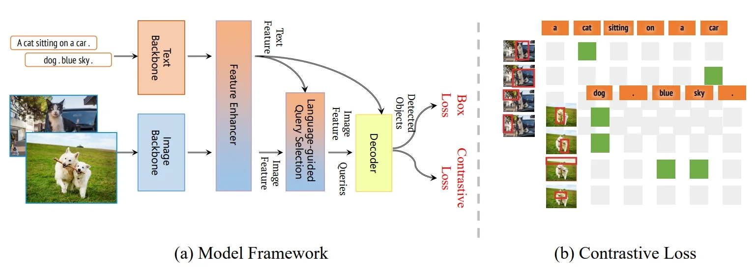
Intuitively, this batch-level contrastive supervision does two things:
- It increases the effective number and diversity of negatives seen per query at each optimization step, beyond what a single image’s prompt can provide.
- It explicitly teaches the model to say “no” to plausible phrases that are valid elsewhere in the batch but not in the current image, which empirically reduces open-vocabulary hallucinations and improves rare-category recall on LVIS [541].
The paper reports consistent gains of roughly \(+1\)–\(2\) AP in zero-shot COCO and on LVIS rare categories when switching from the original image-wise loss to the batch-level variant, under otherwise comparable settings [541].
Scaling axis: Grounding DINO 1.5 Pro On top of the new training recipe, Grounding DINO 1.5 Pro scales the model capacity and data:
- Backbone. The vision backbone is upgraded to ViT-L/14 at higher resolution (e.g., \(336\times 336\)) while keeping the same type of dual-encoder / cross-modality decoder design [541].
- Data. A new Grounding-20M dataset with over 20M grounding images is introduced, substantially enlarging the grounding supervision pool compared to the original Grounding DINO training recipe [541, 384].
- Performance. With batch-level contrastive training and the larger backbone and data, the Pro model reaches around \(54.3\) AP on COCO zero-shot detection and roughly \(55.7\) AP on LVIS-minival zero-shot, a sizeable improvement over the Swin-L version of Grounding DINO and over DetCLIP-style baselines on LVIS [541, 750].
Crucially, these gains do not come from architectural changes in the detector head: the decoder, query formulation, and set-prediction loss remain as in Grounding DINO. The improvements are attributed to (i) the stronger batch-level contrastive training, (ii) the larger ViT-L backbone, and (iii) the much broader grounding corpus.
Efficiency axis: Grounding DINO 1.5 Edge and the efficient feature enhancer While the Pro models target maximal zero-shot and fine-tuned performance, the Edge models target deployment on resource-limited hardware. The main architectural novelty here is an efficient feature enhancer that reduces the cost of encoder fusion:
- Single-scale cross-modality fusion. Instead of running multi-scale deformable self-attention over all feature pyramid levels (e.g., \(P_3\)–\(P_6\)) interleaved with text cross-attention, the Edge enhancer restricts cross-modality fusion to a single high-level feature map (typically the stride-32 \(P_5\) level). Self-attention on this map uses standard multi-head self-attention, which is easier to optimize and deploy than custom deformable kernels.
- External cross-scale injection. Information from lower-level maps \(P_3\) and \(P_4\) is injected into \(P_5\) outside the main cross-modality loop, via lightweight cross-scale fusion (e.g., upsampling and \(1\times 1\) convolutions or simple attention). This preserves multi-scale context without repeatedly applying heavy, multi-level deformable attention.
- Efficient backbone. The image backbone is swapped to EfficientViT-L1, which is specifically designed for fast multi-scale feature extraction on edge devices, while the BERT text encoder and decoder heads follow the original Grounding DINO design [541].
Importantly, the detection formulation remains identical: Edge models still output a set of boxes and phrase scores per image, trained with Hungarian matching, box regression losses, and region-to-token contrastive classification as before. The efficient feature enhancer simply computes the encoder features more cheaply, making it possible to reach, after TensorRT optimization, around \(75.2\) FPS with roughly \(36.2\) AP on LVIS-minival zero-shot on edge-class GPUs [541].
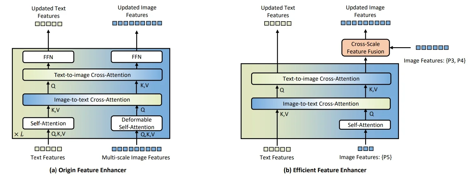
In summary, Grounding DINO 1.5 can be viewed as:
- A training upgrade (batch-level contrastive supervision with richer cross-image negatives) that both Pro and Edge variants share.
- A scaling track (Pro) that combines this training with a ViT-L backbone and a 20M-image grounding corpus for state-of-the-art open-vocabulary performance.
- An efficiency track (Edge) that re-engineers the feature enhancer and backbone for real-time open-set detection on edge devices, without changing the detector head or output format.
Enrichment 14.9.6: Limitations and Outlook
Grounding DINO and Grounding DINO 1.5 illustrate how to integrate a strong DETR-style detector with grounded pre-training for open-set detection, but several limitations remain:
- Prompt-driven hallucination. Like other open-vocabulary detectors and vision–language models, Grounding DINO can still hallucinate objects that are strongly suggested by the prompt but absent in the image (e.g., predicting a “unicorn” box when asked, given a vaguely horse-like shape). Grounding DINO 1.5’s batch-level contrastive training mitigates this by forcing queries to explicitly reject phrases that are correct for other images in the batch but wrong for the current one [541], yet hallucination remains an important open challenge.
- Rare categories and long-tail distributions. On LVIS, Grounding DINO shows significantly lower performance on rare categories compared to frequent ones (e.g., \(18.1\) vs. \(32.7\) AP in a zero-shot Swin-T model) [384]. This reflects both the DETR family’s challenges with rare classes and the limited coverage of rare concepts in available grounding data.
- Box-only outputs. Grounding DINO predicts bounding boxes but not masks. In segmentation pipelines, it must be coupled with models such as Grounded SAM and SAM 2 (in the following chapter on segmentation), which take its boxes as prompts. This decoupling can propagate localization errors to masks.
- Computational cost. Although more efficient than some alternatives (e.g., GLIPv2 and Florence) [789, 768], Grounding DINO still requires substantial pretraining compute and multi-dataset curation. Grounding DINO 1.5 improves training efficiency via batch-level prompting and an efficient feature enhancer [541], but end-to-end open-set detection remains more expensive than closed-set detectors.
- Semantic granularity. Even with sub-sentence prompts, distinguishing fine-grained attributes (e.g., “person wearing a red hat” vs. “person wearing a blue hat”) can be challenging without high-quality attribute-level grounding data.
Despite these limitations, Grounding DINO establishes a compelling template for open-set detectors:
- Combine a strong DETR-style detector (here, DINO-DETR) with grounded language pre-training.
- Use deep cross-modal fusion in the encoder, text-guided query selection, and cross-modality decoding.
- Scale training with batch-level contrastive objectives, as in Grounding DINO 1.5.
Subsequent enrichments in this chapter (OWL-ViT and OWLv2) will show complementary approaches that rely more heavily on CLIP-style vision–language encoders and less on DINO-DETR-style detection heads, providing a broader view of the open-set detection design space.
Enrichment 14.10: OWL-ViT: Open-Vocabulary Detection with ViTs
Enrichment 14.10.1: Motivation and context
OWL-ViT (“Open-World Localization Vision Transformer”) [446] shows that a pure image–text contrastive model, pre-trained only on image-level captions and without any box supervision, can serve as a strong backbone for an open-vocabulary detector once lightweight detection heads are attached and fine-tuned on box-level annotations. This stands in contrast to DINO-DETR [337] and Grounding DINO [384]:
- DINO-DETR is a closed-set detector trained with a deformable encoder–decoder Transformer and Hungarian set prediction loss, using fixed class embeddings and no language information.
- Grounding DINO injects text tokens into both the encoder and decoder, performing deep early fusion between vision and language and learning the detector jointly on caption and grounding corpora.
- OWL-ViT, by contrast, starts from a contrastively pre-trained vision–language model (LiT / CLIP) and keeps its image and text encoders largely decoupled during detection fine-tuning: images go through a ViT, queries go through a text Transformer, and they only meet at the very last layer via dot products.
This late-fusion design has a practical advantage over Grounding DINO: image embeddings can be precomputed and indexed offline, while text prompts can be embedded on the fly. In large-scale retrieval or detection-as-search scenarios, this enables querying new categories without re-running the vision backbone for the entire corpus, which is not possible with Grounding DINO’s tightly coupled encoder–decoder design.
Enrichment 14.10.2: Method
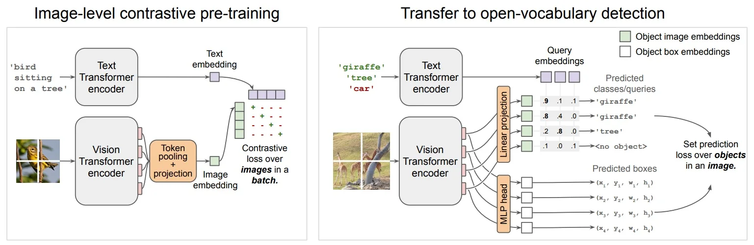
Figure 14.48 summarizes OWL-ViT’s two-stage recipe:
- 1.
- Stage 1: Image-level contrastive pretraining (offline). Before any detection data or bounding boxes are used, OWL-ViT starts from a generic dual-encoder vision–language model trained on large-scale image–caption pairs with a CLIP/LiT-style contrastive objective [512, 779, 446]. A Vision Transformer [134] processes each image \(x\) into a sequence of visual tokens (patch embeddings, optionally preceded by a [CLS] token). These token representations are then collapsed into a single global image embedding \(z^v \in \mathbb {R}^D\), either by reading out the [CLS] token (CLIP-style) or by Multi-head Attention Pooling (MAP, LiT-style) [779], where a few learnable pooling queries attend over all spatial tokens. The text encoder \(f_t\) works in an analogous way: it receives the entire caption \(c\) as a token sequence (e.g., “a bird sitting on a tree”), produces a sequence of hidden states, and then uses a designated final token (the end-of-sequence, EOS, state) as the global caption embedding \(z^t \in \mathbb {R}^D\). Internally, every text token is represented in the same \(D\)-dimensional space, but only this EOS-like summary vector participates in the contrastive loss. Both \(z^v\) and \(z^t\) are \(\ell _2\)-normalized, and a symmetric InfoNCE loss pulls \(z^v\) toward its paired \(z^t\) and pushes it away from other captions in the batch, and symmetrically for \(z^t\). This stage therefore learns a shared \(D\)-dimensional embedding space for global images and global captions only: there is no region-level supervision, no phrase-level supervision, and no bounding box annotations at all. Pretraining is run to convergence on billions of image–text pairs, yielding generic encoders \(f_v\) and \(f_t\) that map images and text sequences to vectors in the same space; these encoders are later reused (or replaced by public CLIP checkpoints) when OWL-ViT is trained as a detector.
- 2.
- Stage 2: Transfer to open-vocabulary detection (task-specific
fine-tuning). After Stage 1 has converged (or when starting from a
pre-existing CLIP/LiT checkpoint), the global pooling used for the
contrastive head (MAP or [CLS]-based readout) is discarded, and the
pretrained ViT trunk is repurposed as a dense feature extractor. The
sequence of visual tokens \(H^v = \{h^v_i\}_{i=1}^N\) is reshaped into an \(H \times W\) grid, and two lightweight
heads are attached directly to each token so that every token acts as a
candidate object prediction. The box regression head is a small MLP
that predicts offsets and log-scales relative to a fixed prior box centered
at the token’s grid location; by adding a bias so that the default box
is centered on the corresponding image patch, OWL-ViT learns only
local deformations around this prior, introducing a strong “location
bias” that stabilizes localization and speeds up convergence [446]. For
classification, each token representation \(h^v_i\) is linearly projected into the
shared \(D\)-dimensional image–text embedding space to yield \(z_i \in \mathbb {R}^D\). Query
strings \(q_k\) (category names, short phrases, or captions) are passed
through the same text encoder \(f_t\) as in Stage 1; for each query, the
final EOS state is taken, projected (if needed), and \(\ell _2\)-normalized to
obtain a query embedding \(e_k \in \mathbb {R}^D\). Thus both \(z_i\) and \(e_k\) live in exactly the same
\(D\)-dimensional space, and classification reduces to a temperature-scaled
cosine similarity \(s_{ik} \propto z_i^\top e_k\) between token \(i\) and query \(k\). For each training
image, the per-image query set consists of all categories annotated
as present or explicitly absent in that image, plus a random sample
of additional category names from the global federated vocabulary
(Objects365, Visual Genome, and related datasets), so that each image
sees on the order of fifty negative categories [446]. Detection training
then fine-tunes the encoders and heads jointly on detection datasets
using a DETR-style bipartite matching loss [64]: Hungarian matching
assigns each ground-truth box to at most one token prediction, \(\ell _1\) and
generalized IoU losses supervise box regression for matched pairs, and
a sigmoid focal loss over the per-image query set handles the large,
federated, partially annotated label spaces.
In practice, the new detection heads use relatively large learning rates, while the pretrained image and text encoders are updated with substantially smaller learning rates, so Stage 2 gently adapts the global image–text space from Stage 1 while endowing individual ViT tokens with localized, open-vocabulary detection capability.
Pretraining: global contrastive alignment (CLIP / LiT style) Let \(f_v\) denote the ViT image encoder and \(f_t\) the text encoder. Given an image \(x\), the ViT processes it into a sequence of patch tokens \[ H^v = \{h^v_1,\dots ,h^v_N\} \in \mathbb {R}^{N \times D_v}, \] where \(N\) is the number of patches and \(D_v\) the hidden dimension. To apply an image-level contrastive loss, these tokens must be aggregated into a single global image representation \(z^v\). OWL-ViT follows the contrastive “dual encoder” setups of CLIP and LiT, and therefore supports two aggregation strategies depending on the underlying pretraining recipe [512, 779]:
- [CLS] token pooling (CLIP-style). For CLIP-based checkpoints, a learnable [CLS] token is prepended to the patch sequence. After the final Transformer block, its hidden state is taken (after layer normalization and a linear projection) as the global image embedding \(z^v\).
- Multi-head Attention Pooling (MAP, LiT-style). For LiT-style pretraining [779], OWL-ViT instead uses Multi-head Attention Pooling (MAP) [779] to aggregate patch tokens. A small set of learnable pooling queries \(Q_{\mbox{pool}} \in \mathbb {R}^{M \times D_v}\) attends over the patch tokens via multi-head attention: \[ O_{\mbox{pool}} = \mathrm {MHA}\bigl (Q_{\mbox{pool}},\, K = H^v,\, V = H^v\bigr ) \in \mathbb {R}^{M \times D_v}. \] The \(M\) pooled outputs are then averaged (or linearly combined) to form \(z^v \in \mathbb {R}^{D_v}\). Intuitively, MAP allows the model to “look back” at all spatial locations with several learnable queries, and to combine them into a global summary that can, for example, focus more strongly on salient foreground objects than on background.
In both cases, the text encoder maps the caption \(c\) to a single caption embedding \(z^t \in \mathbb {R}^{D}\), typically taken from the final end-of-sequence (EOS) token. Both \(z^v\) and \(z^t\) are projected into a shared space of dimension \(D\) and \(\ell _2\)-normalized. For a batch of \(B\) image–caption pairs \(\{(x_b, c_b)\}_{b=1}^B\), OWL-ViT uses the symmetric CLIP/LiT InfoNCE loss [512, 779]: \[ \mathcal {L}_{\mbox{pretrain}} = \frac {1}{2}\,\mathcal {L}_{\mbox{i}\rightarrow \mbox{t}} + \frac {1}{2}\,\mathcal {L}_{\mbox{t}\rightarrow \mbox{i}}, \] where, writing \(s_{uv} = \frac {1}{\tau } (z^v_u)^\top z^t_v\) for a learned temperature \(\tau \), \[ \mathcal {L}_{\mbox{i}\rightarrow \mbox{t}} = -\frac {1}{B}\sum _{b=1}^B \log \frac {\exp (s_{bb})}{\sum _{j=1}^B \exp (s_{bj})}, \quad \mathcal {L}_{\mbox{t}\rightarrow \mbox{i}} = -\frac {1}{B}\sum _{b=1}^B \log \frac {\exp (s_{bb})}{\sum _{j=1}^B \exp (s_{jb})}. \] This aligns each image embedding with its own caption and repels it from all other captions (and symmetrically for captions). Crucially, this stage is purely global: the model never sees bounding boxes or region–phrase pairs, and has no notion of object location yet. All localization ability is introduced only in the second, detection-specific stage.
Detection head: encoder-only dense prediction with location bias To convert the pretrained encoders into an open-vocabulary detector, OWL-ViT removes the global pooling (MAP or [CLS]-based) and retains the full grid of ViT output tokens as dense features. For an input image resized to a fixed resolution (e.g., \(768\times 768\)), the last ViT block produces a sequence \[ H^v = \{h^v_1,\dots ,h^v_N\},\quad h^v_i \in \mathbb {R}^{D_v}, \] which can be reshaped into a 2D grid (e.g., \(24\times 24\) tokens for ViT-B/32). OWL-ViT then attaches two lightweight heads to each token, turning every token into a candidate prediction:
- Box regression head with location bias. A small MLP \(\mathrm {MLP}_{\mbox{box}}\) takes \(h^v_i\) and predicts four real-valued offsets \[ (\Delta c_x,\Delta c_y,\Delta \log w,\Delta \log h)_i = \mathrm {MLP}_{\mbox{box}}(h^v_i). \] Each token \(i\) is associated with a fixed prior center \((c_{x,i}, c_{y,i})\) in image coordinates (obtained by arranging the tokens on a regular grid) and a prior scale \(s_i\) proportional to the patch size / feature stride. The final box prediction \(\hat {b}_i = (\hat {c}_{x,i},\hat {c}_{y,i},\hat {w}_i,\hat {h}_i)\) is obtained as \[ \hat {c}_{x,i} = c_{x,i} + s_i \,\Delta c_x,\quad \hat {c}_{y,i} = c_{y,i} + s_i \,\Delta c_y,\quad \hat {w}_i = s_i \exp (\Delta \log w),\quad \hat {h}_i = s_i \exp (\Delta \log h). \] In other words, before learning, the box for token \(i\) is biased to be centered on its own grid patch with size proportional to that patch; the network only needs to learn local deformations around this default anchor, similar in spirit to Region Proposal Networks [538]. This location bias significantly accelerates convergence and improves final AP compared to predicting absolute coordinates from scratch [446].
-
Classification via text-derived weights and sampled negatives. Instead of learning a fixed classifier over a closed label set, OWL-ViT reuses the shared image–text embedding space learned during contrastive pretraining. A linear projection \(W_{\mbox{cls}}\) maps each visual token to a per-object embedding \[ z_i = W_{\mbox{cls}} h^v_i \in \mathbb {R}^{D}, \] followed by \(\ell _2\)-normalization. A text query \(q_k\) (category name, phrase, or short description) is encoded by the same text encoder, \[ e_k = \frac {f_t(q_k)}{\|f_t(q_k)\|_2} \in \mathbb {R}^D, \] and acts as the classifier weight vector for “class” \(k\). The logit for token \(i\) and query \(k\) is a temperature-scaled cosine similarity \[ s_{ik} = \frac {1}{\tau }\, z_i^\top e_k, \] where the temperature \(\tau \) is inherited from pretraining and optionally fine-tuned. There is no explicit background neuron. Instead, OWL-ViT uses independent sigmoid focal losses over a per-image query set, and a token is treated as background at inference time if its maximum score over all queries falls below a confidence threshold.
For each training image, the per-image query set is constructed from the federated vocabulary as follows [446]:
- All categories annotated as present in the image (positives).
- All categories annotated as absent (known negatives), where such annotations are available.
- Additional “pseudo-negative” categories randomly sampled from the global federated label space (Objects365, Visual Genome, and possibly LVIS/COCO) until each image sees at least about 50 negative categories.
These sampled negatives are crucial: by repeatedly presenting category names that do not match the image, the detector learns to drive their logits down, which is what enables robust open-vocabulary rejection rather than over-triggering on rare classes.
The resulting architecture is an encoder-only, dense detector: there is no Transformer decoder and no learned object queries. However, OWL-ViT still follows DETR’s set-prediction paradigm by using a bipartite matching loss between the \(N\) token-level predictions and the (typically much smaller) set of ground-truth objects [64].
Training objective and federated label spaces Detection training primarily uses Objects365 and Visual Genome with their native label vocabularies and then evaluates on LVIS and COCO [446]. The overall training loop mirrors DETR’s bipartite matching formulation [64], but replaces softmax with sigmoid focal classification and treats the label space in a federated manner.
For a given training image, let \(\{b_j, \mathcal {C}_j\}_{j=1}^M\) denote the \(M\) ground-truth objects, where \(b_j \in \mathbb {R}^4\) are bounding boxes and \(\mathcal {C}_j \subseteq \mathcal {V}_d\) is the (possibly multi-label) set of categories annotated for object \(j\) in the source dataset vocabulary \(\mathcal {V}_d\). Let \(\mathcal {Q} \subseteq \mathcal {V}\) be the per-image query set used for this image; it is constructed as in [446] by combining:
- All categories annotated as present (\(+\)) or explicitly absent (\(-\)) in the image (from \(\mathcal {V}_d\)).
- Additional “pseudo-negative” categories sampled from the global federated vocabulary \(\mathcal {V}\) until there are at least about 50 negatives per image.
For each query \(k \in \mathcal {Q}\), the text encoder \(f_t\) produces an embedding \(e_k \in \mathbb {R}^D\), and the detector produces logits \(s_{ik}\) for each token \(i \in \{1,\dots ,N\}\) as in the previous paragraph.
Bipartite matching. Following DETR, OWL-ViT computes a bipartite matching between the \(M\) ground-truth objects and the \(N\) token-level predictions using the Hungarian algorithm [64]. Let \(\hat {b}_i\) be the predicted box for token \(i\) and let \(\sigma \) be the optimal matching \[ \sigma : \{1,\dots ,M\} \rightarrow \{1,\dots ,N\} \cup \{\varnothing \}, \] that minimizes a matching cost \[ \mathcal {L}_{\mbox{match}}(j,i) = \lambda _{\mbox{cls}}\, \mathcal {L}_\mbox{cls}^{\mbox{match}}(j,i) + \lambda _{\ell _1}\, \|\hat {b}_i - b_j\|_1 + \lambda _{\mbox{giou}}\, \mathcal {L}_{\mbox{giou}}(\hat {b}_i, b_j), \] where \(\mathcal {L}_{\mbox{giou}}\) is the generalized IoU loss [544]. In practice, the weights \((\lambda _{\mbox{cls}},\lambda _{\ell _1},\lambda _{\mbox{giou}})\) are chosen following DETR-style practice; see Minderer et al. [446] for the exact values.
Focal classification loss. For classification, OWL-ViT uses sigmoid focal cross-entropy [368] instead of softmax, to support multi-label annotations and per-image query sets. For a logit \(s_{ik}\) and binary target \(y_{ik} \in \{0,1\}\), define \[ p_{ik} = \sigma (s_{ik}),\qquad \mathrm {FL}(p_{ik}, y_{ik}) = -\,\alpha \, y_{ik}\,(1-p_{ik})^\gamma \log p_{ik} - (1-\alpha )\,(1-y_{ik})\,p_{ik}^\gamma \log (1-p_{ik}), \] with \((\alpha ,\gamma )\) following the standard RetinaNet-style settings used in the original implementation [446]. Given the matching \(\sigma \), the classification targets are defined as follows. For a matched pair \((j, i = \sigma (j))\) and query \(k \in \mathcal {Q}\), \[ y_{ik} = \begin {cases} 1, & \mbox{if } k \in \mathcal {C}_j, \\ 0, & \mbox{if } k \in \mathcal {Q} \setminus \mathcal {C}_j, \end {cases} \] so the token is trained to be positive for all labels in \(\mathcal {C}_j\) and negative for the remaining queries. For unmatched tokens \(i\) (i.e., \(i \notin \mathrm {Im}(\sigma )\)), all targets are zero, \(y_{ik} = 0\) for all \(k \in \mathcal {Q}\), so they act as “no-object” background. The classification loss for one image is then \[ \mathcal {L}_{\mbox{cls}} = \frac {1}{|\mathcal {Q}|\,N} \sum _{i=1}^{N} \sum _{k \in \mathcal {Q}} \mathrm {FL}\bigl (p_{ik}, y_{ik}\bigr ), \] normalized over all tokens and queries for that image.
Box regression loss. Only matched tokens receive box regression supervision. Writing \(j(i)\) for the unique ground-truth object assigned to token \(i\) by the matching (when it exists), the box loss for one image is \[ \mathcal {L}_{\mbox{box}} = \frac {1}{M} \sum _{j=1}^{M} \Bigl ( \|\hat {b}_{\sigma (j)} - b_j\|_1 + \mathcal {L}_{\mbox{giou}}(\hat {b}_{\sigma (j)}, b_j) \Bigr ), \] with the convention that terms with \(\sigma (j) = \varnothing \) are skipped.
Total detection loss and federated masking. The total detection loss for one image is \[ \mathcal {L}_{\mbox{det}} = \lambda _{\mbox{cls}}\, \mathcal {L}_{\mbox{cls}} + \lambda _{\ell _1}\, \mathcal {L}_{\ell _1} + \lambda _{\mbox{giou}}\, \mathcal {L}_{\mbox{giou}}, \] where \(\mathcal {L}_{\ell _1}\) and \(\mathcal {L}_{\mbox{giou}}\) are the \(\ell _1\) and gIoU components of \(\mathcal {L}_{\mbox{box}}\). Because federated datasets such as Objects365, Visual Genome, and LVIS annotate overlapping but non-identical label vocabularies, OWL-ViT computes classification losses only over the per-image query set \(\mathcal {Q}\) for the current dataset and masks gradients for categories outside this vocabulary. This loss masking prevents the model from interpreting unannotated objects as negatives for labels defined only in other datasets (e.g., a “car” present but unannotated in Visual Genome must not be treated as negative evidence for the LVIS “car” class), while still benefiting from additional pseudo-negative queries sampled from the global vocabulary.
Image- and text-conditioned detection A key advantage of OWL-ViT’s symmetric design is that both image and text can act as queries without architectural changes. For text-conditioned detection, class names or phrases are encoded with \(f_t\) and used directly as classifier weights. For image-conditioned detection, a reference image (or a crop) is passed through the same vision encoder \(f_v\), and MAP produces a global embedding that is used as a query vector. When multiple reference images are available, their embeddings are mean-pooled to form a single query.
The following figure shows qualitative one-shot image-conditioned detections: OWL-ViT correctly selects instances of the reference species even when text prompts fail for fine-grained categories.
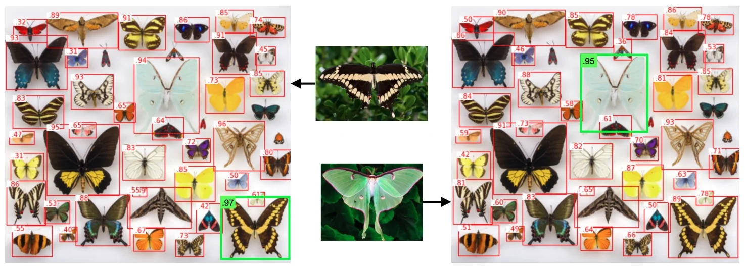
Enrichment 14.10.3: Architecture variants and ablations
The authors evaluate three backbone families: pure ViT backbones (B/32, B/16, L/16, H/14), hybrid CNN+ViT backbones (denoted hybridCNN, where a ResNet trunk produces a convolutional feature map that is flattened into tokens and fed to a ViT head), and pure ResNet-only models. The following figure summarizes two consistent trends:
- For small model sizes and tight FLOPs budgets, hybridCNN backbones (ResNet trunk + ViT head) are more compute-efficient than pure ViTs, achieving competitive AP at lower cost.
- As the FLOPs budget grows, pure ViTs scale better: they reach higher AP on LVIS overall and, more importantly, systematically achieve higher zero-shot AP on LVIS rare categories than both hybridCNN and pure ResNet backbones, indicating a stronger bias toward semantic generalization (reasoning about unseen categories) rather than just localizing a fixed set of known classes.
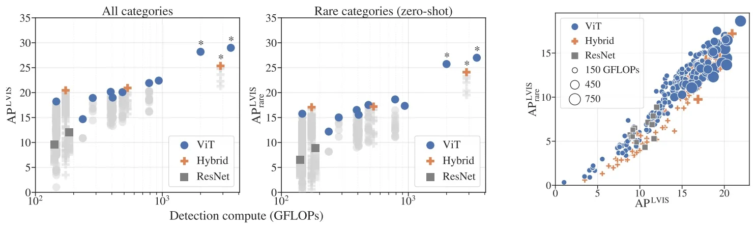
Scaling and transfer from image-level to object-level performance A central empirical question is whether better image-level contrastive pretraining actually translates into better open-vocabulary detection. The following figure plots zero-shot ImageNet accuracy (after pretraining) vs. zero-shot LVIS AP on rare categories (after detection fine-tuning) across many pretraining configurations (backbone type, model size, image resolution, number of pretraining examples).
Two patterns emerge:
- High image-level performance is necessary but not sufficient for high object-level performance: the correlation between pretraining and LVIS rare AP is strong but imperfect (Pearson \(r \approx 0.73\)).
- The right-hand plots show that, for a fixed architecture, longer contrastive pretraining (more image–text examples) improves both ImageNet accuracy and LVIS AP, while additional detection fine-tuning provides a smaller but consistent boost.
These results suggest a kind of lock-in effect: the semantic capacity of the detector is largely determined during image-level pretraining. Fine-tuning on detection data can teach localization, but it cannot easily recover semantic knowledge that the contrastive model never acquired.
Quantitative results on LVIS: open-vocabulary and zero-shot detection The below table summarizes representative LVIS v1.0 validation results from Minderer et al. [446]. Following the paper, \(\mbox{AP}_{\mbox{LVIS}}\) is AP over all categories and \(\mbox{AP}_{\mbox{LVIS}}^{\mbox{rare}}\) measures rare categories; for the zero-shot setting, labels for rare categories are removed from all detection training data.
| Method | Backbone | Training data | \(\mbox{AP}_{\mbox{LVIS}}\) | \(\mbox{AP}_{\mbox{LVIS}}^{\mbox{rare}}\) |
| ViLD-ens [32] | ResNet-50 | LVIS base | 25.5 | 16.6 |
| ViLD-ens [32] | EffNet-B7 | LVIS base | 29.3 | 26.3 |
| RegionCLIP [33] | R50x4-C4 | LVIS base | 32.3 | 22.0 |
| OWL-ViT [8] | ViT-H/14 (LiT) | LVIS base | 35.3 | 23.3 |
| OWL-ViT [8] | ViT-L/14 (CLIP) | LVIS base | 34.7 | 25.6 |
| GLIP [29] | Swin-L | O365 + GoldG + captions | 26.9 | 17.1 |
| OWL-ViT [8] | ViT-B/16 (LiT) | O365 + VG | 26.7 | 23.6 |
| OWL-ViT [8] | ViT-L/16 (LiT) | O365 + VG | 30.9 | 28.8 |
| OWL-ViT [8] | ViT-H/14 (LiT) | O365 + VG | 33.6 | 30.6 |
OWL-ViT thus improves over ViLD and GLIP on both overall AP and zero-shot rare categories, especially when scaled to large ViT backbones and trained on Objects365+VG. For example, the ViT-H/14 LiT model achieves \(33.6\) \(\mbox{AP}_{\mbox{LVIS}}\) and \(30.6\) \(\mbox{AP}_{\mbox{LVIS}}^{\mbox{rare}}\), substantially higher than GLIP’s \(26.9 / 17.1\).
One-shot and few-shot image-conditioned detection on COCO For COCO image-conditioned detection, OWL-ViT compares against SiamMask [246], CoAE (One-Shot Object Detection with Co-Attention and Co-Excitation) [242], and AIT [81]. The following table reports AP\(_{50}\) for seen and unseen category splits.
| Split 1 | Split 2 | Split 3 | Split 4 | Mean | |
Seen categories |
|||||
| SiamMask [49] | 38.9 | 37.1 | 37.8 | 36.6 | 37.6 |
| CoAE [50] | 42.2 | 40.2 | 39.9 | 41.3 | 40.9 |
| AIT [51] | 50.1 | 47.2 | 45.8 | 46.9 | 47.5 |
| OWL-ViT (\(k=1\)) [8] | 49.9 | 49.1 | 49.2 | 48.2 | 49.1 |
| OWL-ViT (\(k=10\)) [8] | 54.1 | 55.3 | 56.2 | 54.9 | 55.1 |
Unseen categories |
|||||
| SiamMask [49] | 15.3 | 17.6 | 17.4 | 17.0 | 16.8 |
| CoAE [50] | 23.4 | 23.6 | 20.5 | 20.4 | 22.0 |
| AIT [51] | 26.0 | 26.4 | 22.3 | 22.6 | 24.3 |
| OWL-ViT (\(k=1\)) [8] | 43.6 | 41.3 | 40.2 | 41.9 | 41.8 |
| OWL-ViT (\(k=10\)) [8] | 49.3 | 51.1 | 42.4 | 44.5 | 46.8 |
On unseen categories, OWL-ViT with a single reference image nearly doubles AIT’s mean AP\(_{50}\) (41.8 vs. 24.3), and using ten reference images further boosts performance to 46.8 AP\(_{50}\).
This illustrates how the symmetric vision encoder can be exploited for powerful image-conditioned detection without modifying the architecture.
Training and data ablations The paper includes a detailed ablation study on LVIS and COCO, varying training data, optimizer settings, prompts, and augmentation [446]. Some key findings (differences relative to a ViT-B/32 baseline trained on O365+VG):
- Training data matters most. Using only Visual Genome captions without Objects365 grounding data reduces \(\mbox{AP}_{\mbox{LVIS}}\) and \(\mbox{AP}_{\mbox{LVIS}}^{\mbox{rare}}\) by roughly 14 points, while using only OpenImages reduces them by about 7 points. Jointly using O365 and VG is important for both breadth and grounding.
- Differential learning rates for image vs. text encoders. Forcing the same learning rate for both encoders significantly hurts rare categories (around \(-8\) points in \(\mbox{AP}_{\mbox{LVIS}}^{\mbox{rare}}\)). In practice, the vision encoder is fine-tuned with a smaller learning rate than the text encoder, similar to domain adaptation methods such as ReCLIP [248].
- Prompt ensembling. Using multiple textual templates (e.g., “a photo of a {class}”, “a {class} in the scene”) and averaging their embeddings improves rare-category AP by around 5 points compared to a single, fixed template.
- Random negative categories. Adding random negative labels per image yields a modest but consistent improvement in zero-shot AP, especially on rare categories, showing that hard negatives sharpen the classifier.
- Mosaic augmentation and localization heuristics. Mosaic-style augmentations and simple heuristics (merging overlapping instances, adding a location bias, filtering cropped boxes) each contribute one or two AP points; removing mosaics harms performance more than simply training for more epochs.
Comparison with Grounding DINO and OWLv2 From the perspective of this chapter, OWL-ViT and Grounding DINO represent two ends of the open-vocabulary detection design space.
- Fusion strategy. OWL-ViT uses late fusion: image and text encoders are independent, and the only interaction is in the dot product between image features and query embeddings at the detection head. Grounding DINO [384] uses early and deep fusion, injecting text tokens into both the encoder and decoder via cross-attention. This makes Grounding DINO stronger at phrase grounding and region–phrase alignment, but also makes it harder to reuse as a stand-alone image or text encoder.
- Backbone training. OWL-ViT relies heavily on large-scale contrastive pretraining and fine-tunes the pretrained ViT and text encoder with relatively small learning rates. Grounding DINO jointly trains (or fine-tunes) its vision backbone and text branch on grounding corpora, often starting from ImageNet- or CLIP-style initialization.
- Detection head. Both models reuse the DETR-style box losses (\(\ell _1\) + GIoU) together with one-to-one Hungarian matching between predictions and ground-truth objects, but Grounding DINO adds a full Transformer decoder with learned object queries, whereas OWL-ViT is encoder-only and uses dense per-patch tokens as predictions.
Subsequent work OWLv2 [445] scales this recipe further with larger backbones, more data, and improved training, pushing LVIS zero-shot performance close to or beyond Grounding DINO while preserving the simplicity and retrieval-friendly, decoupled design.
For example, Minderer et al. report that OWLv2 improves LVIS rare-category AP by more than ten points over the best OWL-ViT v1 configuration, closing most of the gap to fully task-specific detectors.
Enrichment 14.10.4: Limitations and outlook
Despite its strong performance and clean design, OWL-ViT has several limitations:
- Dense, relatively slow inference. Because every ViT patch token predicts a box and scores against all query categories, large OWL-ViT models (e.g., ViT-H/14) can be significantly slower than one-stage CNN detectors, especially when many queries are used. In practice, the authors report a few frames per second on high-end GPUs for large models [446].
- Bounding boxes only. OWL-ViT predicts boxes but not masks. For segmentation, it must be combined with downstream modules such as SAM/SAM2 or Mask DINO (Chapter 15).
- Dependence on pretraining quality. The lock-in effect discussed above means that poor contrastive pretraining cannot be fully compensated during detection fine-tuning. Choosing strong image–text pretraining (e.g., LiT [779], improved CLIP variants, or domain-adapted models such as ReCLIP [248]) is crucial.
- Limited relational reasoning. Purely per-patch scoring against independent queries makes it harder to model relational phrases (e.g., “person holding a red umbrella”) compared to architectures like Grounding DINO that fuse language deeply into the encoder–decoder.
Nonetheless, OWL-ViT has had substantial impact. Its pattern of “frozen vision–language backbone + lightweight detection head with text-derived classifier weights” has been adopted by many later systems, including OWLv2 [445], frozen-VLM detectors, and YOLO-style open-vocabulary models. In later sections, OWLv2 will reappear as a stronger, scaled-up variant that pushes the same design further in both accuracy and robustness.
Enrichment 14.11: OWLv2: Scaling Open-Vocabulary Detection
Enrichment 14.11.1: Motivation and context
OWL-ViT v2 (often abbreviated OWLv2) [445] asks a simple question: if OWL-ViT already turns a contrastively pretrained vision–language model into an open-vocabulary detector, can detection performance be scaled further without collecting more human box annotations. The answer comes from self-training on web data. Instead of hand-labeling new detection datasets, OWLv2 uses OWL-ViT itself as a pseudo-annotator on the WebLI image–text corpus, generating billions of noisy boxes and category labels that are then used to train stronger “student” detectors.
This strategy contrasts with models such as GLIP, DetCLIP, and Grounding DINO [349, 815, 384], which improve open-vocabulary detection primarily by designing more powerful encoder–decoder architectures and pretraining on curated grounding datasets with explicit region–phrase supervision. OWLv2 instead keeps the simple OWL-ViT detection head and late-fusion dual encoders, and concentrates effort on data scaling and training efficiency. The resulting OWL-ST recipe (“OWL Self-Training”) scales to roughly two billion Web images and yields a ViT-G/14 detector with about \(47.2\) AP on rare LVIS categories in the zero-shot setting [445], substantially improving over OWL-ViT v1 while preserving the retrieval-friendly, encoder-only design.
Enrichment 14.11.2: OWLv2: Self-training pipeline (OWL-ST)
Overview of the three-stage recipe OWLv2 (often referred to as OWL-ST in the paper) is best understood as a strictly sequential self-training pipeline built around OWL-ViT [446]. A strong, but relatively expensive, OWL-ViT detector first plays the role of a frozen annotator that pseudo-labels a massive multilingual web corpus (WebLI [275]) with boxes and phrases. A student detector with the same basic architecture but larger backbones (CLIP or SigLIP ViTs) is then trained on these noisy pseudo-boxes using an efficiency-optimized training loop. Finally, for benchmarks such as LVIS, the self-trained student can be optionally fine-tuned on human annotations and weight-ensembled with its pre-fine-tuning version to balance in-distribution accuracy and open-world robustness. Figure 14.52 sketches these stages.
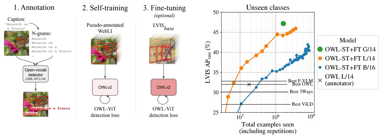
- 1.
- Stage 0: Annotator pretraining (OWL-ViT). The annotator is a standard OWL-ViT detector [446] built on a CLIP ViT-L/14 backbone. It is obtained by first contrastively pretraining CLIP on web-scale image–caption pairs and then training OWL-ViT for detection on human-annotated datasets such as Objects365, OpenImages V4, LVIS, and Visual Genome. This yields a strong open-vocabulary detector that can respond to arbitrary text queries with dense boxes and scores. In principle, any sufficiently strong OWL-ViT variant could serve as annotator, but OWLv2 consistently uses the public CLIP-L/14 OWL-ViT checkpoint in all experiments [445].
- 2.
- Stage 1: Pseudo-annotation of WebLI with the annotator. The frozen OWL-ViT annotator is run on images from WebLI [275], a massive multilingual web image–text collection. For each WebLI image \(x\), OWLv2 must decide which phrases to ask the annotator to look for. It constructs a query list by merging a fixed, human-curated dictionary of standard object categories with image-specific N-grams extracted from the caption: \[ \mathcal {Q}(x) = \underbrace {\mathcal {V}_{\mbox{curated}}}_{\mbox{fixed across images}} \;\cup \; \underbrace {\mathcal {V}_{\mbox{N-gram}}(x)}_{\mbox{caption-derived, image-specific}}. \] OWL-ViT is applied once per image with this merged query list, producing a dense set of candidate boxes and phrase scores. All boxes whose scores exceed a moderate inclusion threshold (e.g., \(0.1\)) are retained as pseudo-annotations, provided the image has at least one prediction above a higher confidence level (e.g., \(0.3\)) [445]. These settings deliberately favor quantity over purity: instead of keeping only the top-1 box per image, OWLv2 harvests many moderately confident boxes, trading some label noise for a huge effective training set.
- 3.
- Stage 2: Self-training the student detector (OWL-ST). A
student detector with the same overall design as OWL-ViT but
larger backbones (e.g., CLIP ViT-G/14 or SigLIP ViT-G/14) is
then trained on the pseudo-labeled WebLI data. In OWLv2’s main
scaling experiments, backbones are initialized from CLIP or SigLIP
checkpoints rather than from the annotator’s detection weights [445],
so the student effectively learns detection “from scratch” under the
supervision of the frozen annotator. Architecturally, the student
remains very simple: a ViT image encoder, a text encoder, and
lightweight per-patch heads. There is no Transformer decoder and no
learnable query embedding set; all predictions are anchored directly
to ViT patch tokens.
Detection objective: dense encoder-only open-vocabulary detection
The OWLv2 detector adopts the encoder-only, one-box-per-token recipe of OWL-ViT [446, 445]: detection heads are attached directly to ViT patch tokens; there is no Transformer decoder. Unlike classic one-stage detectors (e.g., RetinaNet or FCOS), supervision is still formulated as a DETR-style set-prediction problem with bipartite matching rather than heuristic IoU-threshold assignment.
For a training image \(x\) with pseudo-annotations \(\{(b_j, y_j)\}_{j=1}^M\) (pseudo boxes \(b_j\) and phrases \(y_j\) from the OWL-ViT annotator), OWLv2 forms an image-specific query set \[ \mathcal {Q}(x) = \mathcal {V}_{\mbox{curated}} \;\cup \; \mathcal {V}_{\mbox{image}}(x) \;\cup \; \mathcal {V}_{\mbox{neg}}(x), \]
where \(\mathcal {V}_{\mbox{curated}}\) is a fixed vocabulary of human-curated object names, \(\mathcal {V}_{\mbox{image}}(x)\) collects the image-specific phrases that actually appear as pseudo-labels for \(x\) (e.g., N-grams from its WebLI caption or curated names, depending on the pseudo-annotation run), and \(\mathcal {V}_{\mbox{neg}}(x)\) are “pseudo-negative” phrases sampled from other images that are guaranteed never to be positives for \(x\) but act as hard negatives on the text side [445].
All queries \(k \in \mathcal {Q}(x)\) are encoded into text embeddings, and the image is passed through the ViT encoder to yield patch embeddings \(\{h_i\}_{i=1}^N\). On top of each token \(i\) OWLv2 adds three lightweight heads:
- An objectness head predicting a scalar score \(o_i\) that estimates how likely the token corresponds to an object at all.
- A box head predicting a single candidate box \(\hat {b}_i\) (center coordinates and size) for that token.
- A classification head producing logits \(s_{ik}\) for all queries \(k \in \mathcal {Q}(x)\), typically implemented as scaled dot products (equivalently, cosine similarities after \(\ell _2\)-normalization) between visual and text embeddings, as in OWL-ViT.
To reduce computation, OWLv2 computes classification and box losses only for the top-\(K\) tokens by objectness during training (about \(10\%\) of tokens); the objectness head is trained so that tokens which later obtain high classification scores also receive high objectness scores [445].
Training: bipartite matching, not IoU-threshold mining
Let \(\mathcal {I}(x) \subset \{1,\dots ,N\}\) be the top-\(K\) tokens selected by objectness. As in OWL-ViT [446], OWLv2 uses a DETR-style Hungarian matching loss to define positives among these tokens. Concretely, for each image \(x\) the model solves a one-to-one assignment between the \(M\) pseudo boxes \(\{b_j\}\) and the selected tokens \(\{i \in \mathcal {I}(x)\}\): \[ \pi ^* = \arg \min _{\pi } \sum _{j=1}^M \Bigl [ \mathcal {C}_\mbox{cls}\bigl (s_{\pi (j),\,y_j}\bigr ) + \lambda _\mbox{box}\,\mathcal {C}_\mbox{box}\bigl (\hat {b}_{\pi (j)}, b_j\bigr ) \Bigr ], \] where \(\pi \) ranges over one-to-one assignments from boxes to tokens, \(\mathcal {C}_\mbox{cls}\) is the sigmoid / focal classification cost for phrase \(y_j\), and \(\mathcal {C}_\mbox{box}\) combines an \(\ell _1\) distance and a (G)IoU-based cost between \(\hat {b}_i\) and \(b_j\) [446]. Matching is therefore not a pure IoU-threshold rule: the assignment jointly prefers tokens that have both high phrase score and good geometric overlap with the pseudo box.
The resulting permutation \(\pi ^*\) induces binary labels \(t_{ik} \in \{0,1\}\) over all token–query pairs: \[ t_{ik} = 1 \quad \mbox{iff}\quad \exists j \;\mbox{s.t.}\; i = \pi ^*(j) \;\mbox{and}\; k \mbox{ is the query corresponding to } y_j, \] and \(t_{ik} = 0\) otherwise (including all tokens that are unmatched and all negative or pseudo-negative queries). Because each pseudo box \(b_j\) is matched to one token at most, the model is explicitly discouraged from producing many redundant positives around the same object: overlapping tokens compete in the matching, and only the best one is treated as a positive, while the others become background and are down-weighted by the focal loss.
The overall detection loss decomposes into a dense classification term and a regression term applied only to matched tokens: \[ \mathcal {L}_\mbox{det} = \underbrace {\sum _{i \in \mathcal {I}(x)} \sum _{k \in \mathcal {Q}(x)} \mathcal {L}_\mbox{cls}\bigl (s_{ik}, t_{ik}\bigr )}_{\mbox{sigmoid / focal classification over queries}} \;+\; \lambda _\mbox{box} \underbrace {\sum _{j=1}^M \mathcal {L}_\mbox{box}\bigl (\hat {b}_{\pi ^*(j)}, b_j\bigr )}_{\ell _1 + \mathrm {GIoU on matched tokens only}}, \] with a separate loss on the objectness scores \(o_i\) that encourages high objectness precisely for those tokens that end up with strong classification scores [445].
Inference and overlapping boxes
At inference time, no matching is solved: the model runs the encoder once, predicts a box \(\hat {b}_i\) and query logits \(\{s_{ik}\}_{k}\) for (essentially) all tokens, and keeps token–query pairs whose detection score \(\sigma (s_{ik})\) exceeds a threshold for the user-specified queries. Thanks to the one-to-one training objective inherited from OWL-ViT, the model tends to produce at most one high-scoring token per object and query, so heavy non-maximum suppression is not strictly required in the DETR sense. In practice, implementations can still apply light per-query top-\(K\) filtering and/or NMS to prune occasional near-duplicate boxes, especially when many queries are evaluated or when pseudo-labels are noisy.
How can the annotator produce boxes for phrases it never saw during detection training? A subtle but important point is that the OWL-ViT annotator does not rely only on its supervised detection data (Objects365, OpenImages, LVIS, Visual Genome) to recognize concepts. Its visual and textual backbones are initialized from CLIP-style contrastive pretraining on hundreds of millions of image–text pairs, which already align a very broad vocabulary of phrases with corresponding visual patterns [446]. Detection training then mainly teaches OWL-ViT where to put boxes, while its knowledge of what phrases such as “platypus”, “dog wearing sunglasses”, or “rusty bicycle” look like is inherited from this large-scale image–text pretraining.
- Teacher zero-shot capability. Given a caption-derived N-gram such as “dog wearing sunglasses”, OWL-ViT embeds the phrase with its text encoder and compares it to per-patch image features, exactly as in CLIP-style zero-shot classification. Even if no detection dataset ever contained that phrase as a box label, the shared embedding space already makes the corresponding patches stand out, so OWL-ViT can often draw a pseudo-box zero-shot [446, 445]. In other words, detection is treated as localized retrieval inside the image rather than as pure supervised classification over a fixed label set.
- Captions as prompts. The N-gram does not ask the annotator to guess blindly; it acts as an explicit prompt that says “look for this thing in this image”. For example, if the caption contains “two drones flying over a city”, OWL-ViT is directly encouraged to search for regions that match the text “drone”, even if its own detection training never included a dedicated “drone” category. When the phrase genuinely describes something in the image, CLIP-style alignment usually yields at least a roughly correct box.
-
What if the annotator is wrong or misses the object. For any single image, the annotator can certainly fail: it may hallucinate a box for a non-visual phrase (e.g., “click here”), or miss a small, occluded instance entirely. However, WebLI contains the same concept in many different images and captions.
Across thousands of occurrences of “golden retriever” or “drone”, the teacher’s correct localizations are consistent (similar dogs or drones in similar regions), whereas its mistakes are visually diverse and inconsistent.
When the student is trained on billions of such pseudo-labels, gradient descent naturally fits the consistent patterns and fails to fit the idiosyncratic errors, effectively denoising the teacher’s supervision over the whole corpus [445].
Why can OWLv2 outperform its own annotator instead of copying its mistakes? Intuitively, if the student only ever sees the teacher’s outputs, one might worry that it cannot do better than the teacher. OWLv2 overcomes this in three complementary ways.
- Many more (noisy) examples than the annotator ever saw. The annotator was trained on tens of millions of human-labeled boxes. The student, in contrast, is trained on pseudo-boxes for billions of WebLI images (when counting all mosaics and confidence thresholds), which is one to two orders of magnitude more supervision [445]. Even if each pseudo-box is imperfect, the sheer number of partially correct instances for each concept lets the student learn richer and more robust visual features than the annotator ever could.
- Larger backbones and more compute-efficient training. OWLv2 students use larger vision backbones (e.g., SigLIP ViT-G/14) than the CLIP ViT-L/14 annotator, and the Stage 2 training loop (token dropping, objectness-based instance selection, mosaic augmentation) is engineered to push far more data through these large models within a fixed compute budget. Empirically, Minderer et al. show that these students achieve substantially higher LVIS rare-category AP and ODinW mean AP than the original OWL-ViT teacher, even though the teacher provided all pseudo-labels [445].
- Signal versus noise at web scale. For a concept like “hydrant”, the teacher might localize it correctly in many images and miss or mislabel it in others. The correct localizations all share recognizable visual structure, whereas the errors are scattered over unrelated backgrounds. Over billions of examples, the student can only consistently reduce its loss by latching onto the stable pattern (true hydrants) rather than the inconsistent noise. Thus, instead of copying the teacher’s individual mistakes, OWLv2 averages them out and retains only what is statistically supported across the corpus.
What happens to objects that are not in the query set? A complementary concern is how an open-vocabulary detector can handle objects that are present in an image but never appear in that image’s curated+N-gram query list. Here it is crucial that OWLv2 trains conditionally on the query set \(\mathcal {Q}(x)\) of each image [445].
- Conditional supervision per image. For a given training image \(x\), the student is only asked: “Given this particular list of phrases \(\mathcal {Q}(x)\), which tokens correspond to which phrases?”. If “fire hydrant” is not in \(\mathcal {Q}(x)\), then hydrants in that image are simply ignored by the loss for that phrase: they are neither positives nor explicit negatives for “fire hydrant”. The model is not told that hydrants are background; it is merely not supervised about them in this particular image.
-
Coverage across WebLI. Across billions of WebLI images, most semantically meaningful concepts (“hydrant”, “escalator”, ...) do appear as queries in many other images, either via curated labels or via N-grams extracted from captions. Those other images do contribute gradients for these phrases, so the student still receives substantial supervision for each common concept, just not from every image in which it happens to appear.
- Role of CLIP/SigLIP initialization for genuinely rare phrases. For truly rare or unseen phrasings, the CLIP or SigLIP initialization already provides a coarse alignment between text and image embeddings. OWLv2’s self-training mainly improves localization, calibration, and robustness for phrases that the annotator can already tentatively ground. As in CLIP zero-shot classification, entirely new test-time prompts can still be handled if they lie in the semantic neighborhood of phrases seen during pretraining or self-training.
Thus, the absence of a phrase from \(\mathcal {Q}(x)\) for a particular image does not forbid the model from ever detecting that concept; it simply means that this image does not contribute any signal for that phrase. Over the full WebLI corpus, consistent concepts accumulate many positive examples, while idiosyncratic or spurious N-grams (e.g., “click here”) fail to form a coherent visual pattern and are effectively ignored by the student during training.
Scaling the objective to billions of pseudo-boxes. The real difficulty in Stage 2 is not the loss itself but making it computationally feasible to run this dense, open-vocabulary objective on billions of pseudo-labeled images with tens of thousands of queries per image. Minderer et al. therefore introduce three complementary efficiency mechanisms [445]:
- Token dropping (static visual pruning). After a few ViT blocks, OWLv2 computes a simple saliency proxy for each token (per-channel feature variance) and discards the least informative tokens for the remainder of the network. Uniform background patches (sky, walls, large textureless regions) have low variance and are pruned; tokens that carry edges, textures, and object structure are kept. This halves (or more) the sequence length for all subsequent layers and detection heads, cutting FLOPs and memory while preserving object-centric regions.
-
Objectness head and dynamic instance selection. Even after token dropping, naively comparing every remaining token to every query in \(\mathcal {Q}(x)\) is prohibitively expensive when \(|\mathcal {Q}(x)|\) can be \(10^4\)–\(2\times 10^4\). OWLv2 therefore adds a lightweight objectness head that predicts a scalar score for each token [445].
During training, only the top-\(K\) tokens (typically a small fraction of the retained tokens) ranked by objectness are passed through the full open-vocabulary classification head and incur the expensive dot-product loss against all queries in \(\mathcal {Q}(x)\); the box head itself remains dense and is applied to all tokens. Tokens with low objectness are treated as background and bypass the classification head.
Objectness is learned jointly with detection: tokens that are repeatedly associated with pseudo-boxes are encouraged to have high objectness, creating a self-reinforcing mechanism that focuses compute on object-like regions. This strategy focuses computation where objects are likely to appear and largely decouples the training cost from the size of the text vocabulary [445].
-
Mosaic augmentation at web scale. Finally, OWLv2 increases the number of distinct scenes seen per optimizer step using large mosaics: instead of a single WebLI image, the input is a grid (e.g., up to \(6\times 6\)) of different images tiled into one canvas [176, 445]. All pseudo-boxes are geometrically transformed into mosaic coordinates, and the detector is trained as if this were a single large image. In the default configuration, each mosaic contains on average about \(13.2\) raw images. Scaling plots therefore report the total number of raw images seen as \[ \mbox{# raw images seen} \approx 13.2 \times \mbox{(# of mosaics)}. \]
Within a fixed budget of optimizer steps, mosaics allow the student to experience roughly an order of magnitude more distinct scenes than a standard one-image-per-step loop, which is critical for exploiting WebLI’s diversity.
Conceptually, Stage 2 turns OWL-ViT’s pseudo-labels into a dense but noisy supervision signal that a much larger, more compute-efficient student can exploit. Whereas the annotator itself was only trained on tens of millions of human-labeled boxes, the student is exposed to billions of pseudo-boxes covering far more phrases and visual situations than the teacher ever saw [445]. Over this huge dataset, consistent visual–linguistic patterns (e.g., what “dog wearing sunglasses” typically looks like) reinforce one another, while spurious N-grams and mislocalized boxes fail to generalize. Combined with the CLIP/SigLIP initialization and the compute-aware training tricks above, this explains how the OWLv2 student can eventually surpass its OWL-ViT teacher by a large margin on both LVIS rare categories and open-world benchmarks such as ODinW.
- 4.
- Stage 3: Optional fine-tuning and weight ensembling. For standard benchmarks such as LVIS, a self-trained OWLv2 student can optionally be fine-tuned on the target dataset using its native annotations. As observed in robust fine-tuning work [722], this creates a tension: pure self-training yields excellent zero-shot and ODinW performance but underperforms on LVIS base categories, while full fine-tuning improves LVIS AP but partially erodes open-world generalization. OWLv2 addresses this by weight-space ensembling: the final model is a convex combination \[ \theta _{\mbox{ens}} = \lambda \, \theta _{\mbox{ST}} + (1-\lambda )\, \theta _{\mbox{FT}}, \] where \(\theta _{\mbox{ST}}\) and \(\theta _{\mbox{FT}}\) denote the self-trained and fine-tuned checkpoints and \(\lambda \in [0,1]\) controls the trade-off between robustness and in-domain accuracy [445, 722]. By sweeping \(\lambda \), Minderer et al. obtain a Pareto frontier of models that can be tuned to favor LVIS, ODinW, or a balanced mix, all without changing the architecture or retraining from scratch.
These stages are executed strictly in order: pseudo-label generation is performed offline with a frozen OWL-ViT annotator; the student is then trained end-to-end on pseudo-annotations; any dataset-specific fine-tuning and weight ensembling happen only after self-training has converged. There is no joint training of annotator and student, and the annotator is never updated using pseudo-labels.
Enrichment 14.11.3: OWLv2: Pseudo-label spaces and Web-scale annotation
Curated vs. N-gram label spaces A central design question in OWLv2 is which phrases to use when querying the OWL-ViT annotator. Unlike standard detectors with a fixed class list, OWL-ViT can score arbitrary text; OWLv2 exploits this by constructing, for every WebLI image, a query list that mixes human-curated object names with free-form phrases extracted from the caption [445]. Minderer et al. systematically study three label spaces:
- Curated vocabulary. A fixed, human-designed list obtained by merging the category names of standard detection datasets (LVIS, Objects365, OpenImages V4, Visual Genome), followed by simple normalization such as lowercasing and deduplication of synonyms and plural forms (Appendix A.1 of [445]). This yields a few thousand canonical object labels that are shared across all images and closely aligned with evaluation benchmarks such as LVIS and ODinW.
- Machine-generated N-gram vocabulary. For each WebLI image \(x\), OWLv2 extracts word N-grams up to length \(10\) from the associated caption and related text fields, after removing stop words and very generic phrases such as “click here” or file-type indicators, and capping the number of queries per image (Appendix A.2 of [445]). The resulting \(\mathcal {V}_{\mbox{N-gram}}(x)\) is image-specific and captures idiosyncratic phrases that never appear in curated taxonomies, but it also introduces label noise whenever the caption is only weakly related to the visual content.
- Union of curated and N-grams. The two label spaces are combined so that the annotator sees both benchmark-aligned category names and image-specific phrases: \[ \mathcal {Q}(x) = \mathcal {V}_{\mbox{curated}} \cup \mathcal {V}_{\mbox{N-gram}}(x). \] Every OWL-ViT forward pass uses this merged query list; there is no splitting of ground truth by source, and from the student detector’s perspective there is just one pool of pseudo-boxes with associated phrases.
The following figure summarizes quantitatively how these three label spaces affect downstream detection, and in particular how the extra coverage from N-grams trades off against their higher noise level.
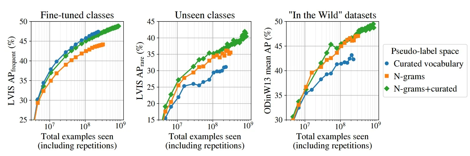
The three panels make the trade-off between clean but narrow and wide but noisy supervision visible:
-
Curated-only (clean but narrow). On LVIS frequent classes (left), the curated-only student achieves the highest or nearly highest AP for a given number of examples, reflecting that curated labels provide relatively clean pseudo-boxes on categories the teacher knows well. On LVIS rare classes and ODinW (middle and right), the same blue curve lags behind, because many long-tail concepts never appear in the curated list at all, so the student simply never receives labels for them.
- N-grams-only (wide but noisy). The N-gram-only student substantially improves AP on LVIS rare and ODinW compared to curated-only, showing that caption-derived phrases do expose the long tail and enable better open-world generalization. At the same time, on LVIS frequent classes its orange curve sits consistently below the blue curve: if N-grams were as clean as curated labels, these curves would coincide. This systematic gap on familiar categories is how the additional label noise introduced by N-grams manifests in the plots.
- Union of curated and N-grams (best trade-off). The union model recovers most of the curated model’s strength on LVIS frequent classes while matching or exceeding the N-gram model on LVIS rare and ODinW. Its green curve is close to blue on the left panel but clearly above both blue and orange in the middle and right panels, indicating that combining an anchored, benchmark-aligned vocabulary with a noisy but broad N-gram explorer yields the best overall balance between precision on known classes and recall on open-world concepts.
Why the union matters: anchor and explorer Using the union of curated and N-gram vocabularies is not redundant; it compensates for complementary failure modes.
- Curated vocabulary as an anchor. Web captions are frequently incomplete or metaphorical: an image can clearly contain a dog while the caption says only “my best friend enjoying the weekend”. If OWLv2 relied only on N-grams, the annotator would be asked to look for “best friend” and “weekend”, but never for the canonical label “dog”. The curated dictionary acts as a safety net: regardless of how the caption is phrased, every image is always queried for common objects such as “person”, “dog”, and “car”, which stabilizes supervision on benchmark-aligned categories and prevents obvious objects from being systematically missed.
- N-grams as an explorer. Conversely, curated lists are static and cannot cover the combinatorial richness of web text. They describe “dog” and “sunglasses” but not necessarily “dog wearing sunglasses” or rare fine-grained entities such as “Monarch on a Zinnia”. N-grams promote these caption phrases to first-class labels, allowing the annotator to create pseudo-boxes for concepts that never appear in any standard taxonomy. Across billions of images, the consistent visual patterns behind phrases such as “drone”, “bento box”, or “steampunk toaster” reinforce each other, whereas non-visual or idiosyncratic phrases fail to form a coherent pattern and are effectively suppressed by scale.
In this sense, the curated vocabulary acts as an anchor that keeps supervision aligned with canonical benchmarks and protects recall on standard categories, while the N-grams act as an explorer that pushes supervision into the long tail of web concepts; the union label space lets the student benefit from both.
Effect of pseudo-label confidence thresholds on downstream detection The label space determines what can, in principle, be labeled; confidence thresholds determine how much of that potential supervision survives filtering. OWLv2 therefore ablates the confidence threshold \(\tau \) used to keep OWL-ViT pseudo-boxes, training otherwise identical students with \(\tau \in \{0.1, 0.3, 0.5, 0.7\}\) and evaluating them on LVIS and ODinW [445].
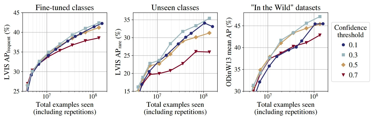
Reading Figure 14.54 from left to right, each curve first improves as the student sees more pseudo-labeled examples and then gradually saturates once the available pseudo-labels have been revisited many times. The position and height of this saturation encode how OWLv2 trades off label quality against scale:
- High thresholds shrink the dataset and hurt generalization. The red curves corresponding to \(\tau = 0.7\) consistently saturate earliest and at the lowest AP, especially for LVIS rare classes and ODinW. Minderer et al. report that increasing \(\tau \) from \(0.1\) to \(0.7\) reduces the number of usable WebLI images from roughly \(5\) billion to a few hundred million. After this smaller pool has been seen a few times, the student runs out of new, informative examples, and the red curves flatten while others continue to improve.
-
Moderate thresholds keep hard examples without collapsing under noise. The blue and gray curves corresponding to \(\tau = 0.1\) and \(\tau = 0.3\) remain the highest in the “Unseen classes” and “In the Wild” panels, while matching the best performance on frequent LVIS classes.
Lower thresholds admit many more medium-confidence detections, which include a mix of genuinely hard positives and some false positives. If this additional supervision were dominated by noise, these curves would deteriorate or oscillate; instead, their steady upward trend indicates that, at WebLI scale, the student successfully averages out inconsistent labels while benefiting from the extra diversity.
-
Noise manifests primarily as an efficiency penalty. When we compare low-threshold curves (e.g., \(\tau = 0.1, 0.3\)) against stricter ones at the same position on the \(x\)-axis early in training, the low-threshold models sometimes lag slightly behind. This is the cost of noise: the student must process more pseudo-labeled examples to statistically separate signal from spurious boxes. Crucially, these curves do not saturate prematurely. As training continues and more examples are seen, the low-threshold models overtake the high-threshold ones and reach higher final AP.
Thus, in OWLv2 the additional noise from low thresholds is not a hard ceiling on performance, but an efficiency penalty that WebLI’s scale can amortize.
Together, the label-space and threshold ablations support OWLv2’s overall philosophy. A broad union label space ensures that most semantically meaningful concepts can, at least sometimes, be named and localized, while low-to-moderate confidence thresholds maximize the number and diversity of training examples. Because the student can process WebLI at this scale (using dense one-stage training, token dropping, objectness-based instance selection, and mosaic augmentation), it is able to distill a noisy but extremely rich pseudo-label stream into detectors that outperform their OWL-ViT teachers on both benchmark categories and truly in-the-wild objects.
Enrichment 14.11.4: Architecture and training efficiency
Student detector: OWL-ViT with efficiency tweaks The student detector in OWLv2 retains the basic OWL-ViT structure [446]: a ViT image encoder \(f_v\), a text encoder \(f_t\), and lightweight box and classification heads attached to per-patch visual tokens. The detection objective is the same dense one-stage loss as in OWL-ViT: open-vocabulary sigmoid (often focal) classification over a per-image query set, combined with \(\ell _1\) and generalized IoU losses on bounding boxes, with positives defined by an IoU threshold (e.g., \(\ge 0.5\)) between predicted and (pseudo) ground-truth boxes [446, 445]. There is no Transformer decoder and no Hungarian matching; supervision is fully dense over the patch grid. Queries include both positive category names and randomly sampled “pseudo-negative” labels from other images, just as in OWL-ViT.
What changes in OWLv2 is how this detector is trained at web scale. The main additions are:
- Token dropping for cheap ViT forward passes and lower memory use.
- An objectness head for focusing classification on likely object patches.
- Mosaic augmentation to expose the student to far more distinct images per training step.
Token dropping OWLv2 adopts a form of dynamic token sparsification inspired by methods such as DynamicViT and Token Merging [528, 49]. After a subset of early Transformer blocks, the model computes a simple saliency score for each patch token, for example based on its feature variance across channels, and drops a fixed fraction (e.g., \(50\%\)) of the least informative tokens from subsequent layers [445]. This reduces the number of tokens processed by later, more expensive layers without modifying the underlying ViT backbone or its final feature stride. During self-training, token dropping provides a substantial reduction in FLOPs and memory; at inference time, the full set of tokens can be used.
Objectness head and instance selection Running open-vocabulary classification against a very large label space (hundreds of thousands of queries) for every token is prohibitively expensive. To decouple training cost from vocabulary size, OWLv2 adds an objectness head that predicts a scalar objectness score for each token. During self-training, only the top fraction of tokens by objectness (roughly \(10\%\) in the experiments) are passed through the full classification head and incur the expensive open-vocabulary loss [445].
Importantly, objectness is itself learned. Its supervision signal comes from the eventual classification scores: tokens that repeatedly receive high classification probabilities for some query are encouraged to have high objectness, so the objectness head learns to anticipate where interesting objects are likely to appear. This mechanism is reminiscent of efficient DETR variants that use dense objectness priors to restrict decoding to promising locations [752], but adapted to the encoder-only, patch-based setting of OWL-ViT.
Mosaic augmentation and the “13.2\(\times \)” factor To maximize the number of distinct images seen under limited training steps, OWLv2 uses large mosaic grids that tile multiple WebLI images into a single training example. Similar to copy-paste and mosaic augmentations used in CNN detectors, grids of varying sizes (e.g., \(1\times 1\) to \(5\times 5\)) are sampled, and pseudo-boxes are geometrically transformed into the corresponding mosaic coordinates [445].
In the configuration used for the main scaling experiments, a single mosaic contains on average about \(13.2\) distinct raw images. Mosaics thus allow the student to process roughly an order of magnitude more images than a standard single-image training loop within the same compute budget. Consequently, the “total examples seen” reported on the \(x\)-axis of the scaling plots should be interpreted as the effective number of raw images processed (approximately \(13.2\times \) the number of optimizer steps).
Enrichment 14.11.5: Scaling behavior, results, and trade-offs
Scaling laws and “student surpasses teacher” One of the main contributions of OWLv2 is an empirical study of scaling laws for open-vocabulary detection under self-training. The following figure illustrates performance (e.g., LVIS rare AP) against the total number of WebLI examples seen during self-training, for several model sizes and architectural variants.
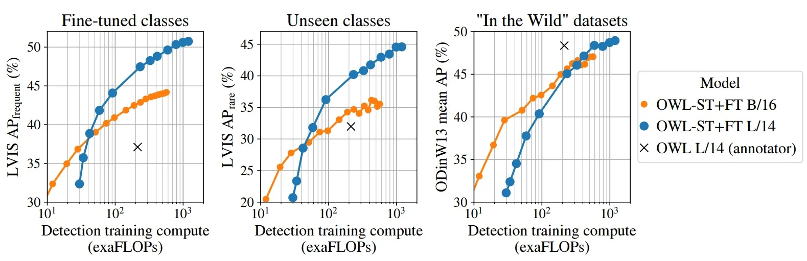
Several consistent patterns emerge [445]:
- Self-training is beneficial even at moderate compute. For reasonable training budgets, students already outperform the frozen OWL-ViT annotator that generated their pseudo-labels, demonstrating a clear “student surpasses teacher” effect.
-
Detection exhibits familiar log-linear scaling. As in large-scale classification and language modeling, performance grows roughly log-linearly with compute and data once models are in the high-data regime.
- Model size vs. training duration trade-off. For in-distribution benchmarks such as LVIS, larger backbones (e.g., ViT-L/14) dominate smaller ones once sufficient data is seen, but for heavily out-of-distribution settings (ODinW), it can be better to train a smaller backbone for longer rather than a larger one for fewer updates.
- Largest model. A SigLIP ViT-G/14 student trained with OWL-ST reaches mid-\(40\) AP on LVIS rare categories (around \(46\)–\(47\) AP depending on the exact training and ensembling setup), which at the time of publication represents one of the strongest reported LVIS rare results among open-vocabulary detectors [445].
Fine-tuning vs. open-world generalization Like many contrastively trained vision–language models, OWLv2 exhibits a trade-off between performance on a specific target dataset and robustness to distribution shift [512, 722]. The below figure illustrates this trade-off using LVIS (target dataset) and ODinW13 (out-of-distribution benchmark).
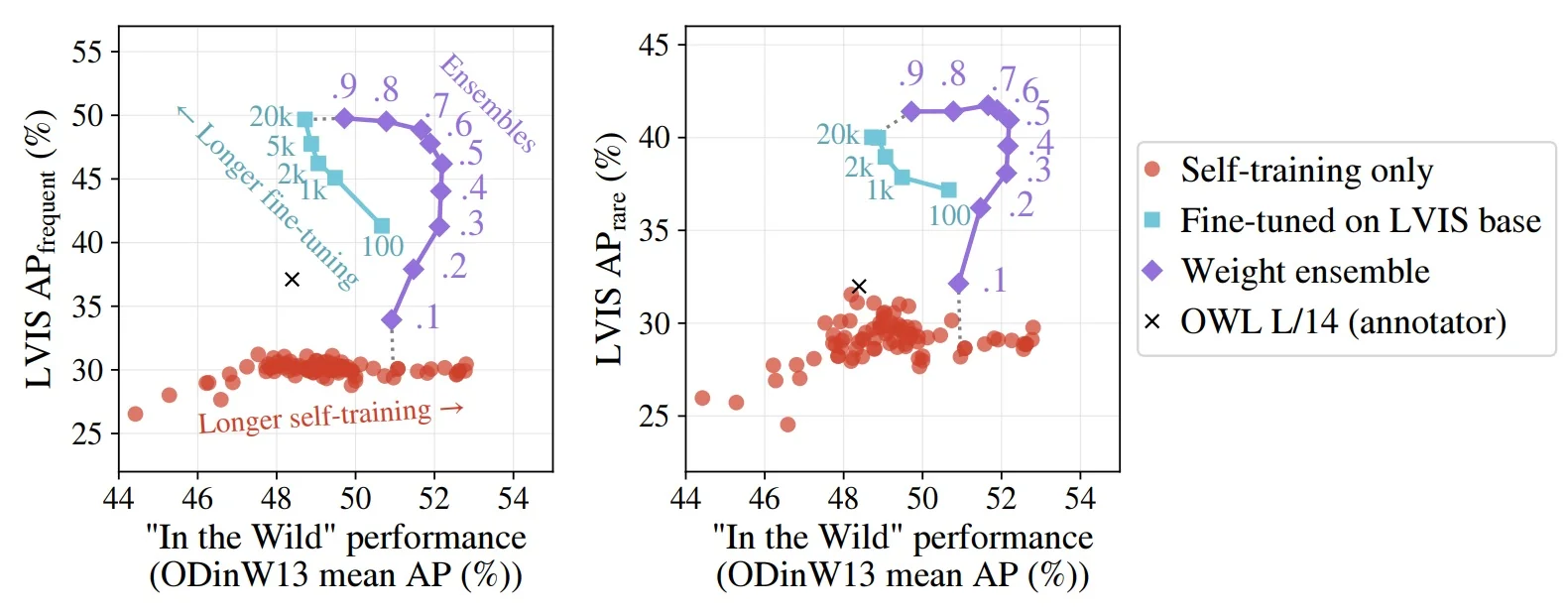
Without fine-tuning, OWLv2 models already deliver strong zero-shot performance across many datasets (LVIS, ODinW13, Objects365, OpenImages) thanks to the diversity of WebLI pseudo-annotations. Fine-tuning on LVIS further boosts performance on LVIS categories but tends to degrade open-world generalization. Weight-space ensembling between self-trained and fine-tuned checkpoints offers a simple way to shift this trade-off, recovering much of the ODinW performance while maintaining high LVIS AP [445].
Enrichment 14.11.6: Comparison to Grounding DINO and limitations
OWL-ViT / OWLv2 vs. Grounding DINO From the perspective of Chapter 14, OWLv2 and Grounding DINO [384] represent two complementary strategies for scaling open-vocabulary detection.
- Architecture and fusion. Grounding DINO starts from a DINO-DETR-style encoder–decoder with multi-scale deformable attention and injects text tokens deep into both encoder and decoder via cross-attention, enabling strong phrase grounding and fine-grained region–text alignment. By contrast, OWLv2 retains OWL-ViT’s dual-encoder, late-fusion design: image and text are encoded separately and only interact in the final dot-product similarity between per-patch features and query embeddings. This makes OWLv2 much closer to CLIP-style retrieval models and simplifies reuse of the encoders for other tasks.
- Training data. Grounding DINO relies on curated grounding datasets (e.g., Objects365, GoldG, Cap4M) with box-level text supervision [384]. OWLv2’s main gains come from scaling to roughly two billion pseudo-annotated WebLI images, produced automatically from captions with minimal filtering [445].
- Inference behavior. Grounding DINO’s tightly coupled encoder–decoder must be re-run whenever the text prompt changes, which can be expensive when exploring many complex prompts. OWLv2 inherits OWL-ViT’s decoupled, encoder-only inference: image features can be precomputed and indexed, while new text queries are embedded on the fly. This is advantageous for large-scale retrieval and detection-as-search applications.
- Performance. At publication time, OWLv2’s SigLIP ViT-G/14 student achieved state-of-the-art zero-shot rare-category AP on LVIS, substantially outperforming OWL-ViT v1 and strong baselines such as F-VLM and DetCLIP [322, 749, 445]. Grounding DINO remains competitive and often superior for phrase-level grounding and tasks that require tight coupling between language and detection, especially when trained with strong region–phrase supervision.
Limitations and outlook Minderer et al. highlight several limitations of OWLv2 [445].
- Compute and data cost. Self-training at the scale of billions of images and large ViT backbones demands substantial compute and infrastructure. Scaling further is in principle effective but quickly becomes impractical without more efficient architectures or training recipes.
- Trade-off between specialization and robustness. Fine-tuning on a target detection dataset improves performance on its label space but reduces robustness to distribution shift and sensitivity to prompt wording, similar to CLIP fine-tuning [722]. Weight ensembling mitigates but does not completely remove this trade-off.
- Noise and bias in pseudo-labels. Although OWLv2 shows that simple pseudo-annotations can be surprisingly effective at scale, they still inherit biases from the annotator, the label space, and the WebLI corpus. Improving pseudo-label quality or incorporating uncertainty estimates could further enhance performance.
Despite these limitations, OWLv2 demonstrates that a relatively simple OWL-ViT-style detector, combined with web-scale self-training, can close much of the gap to more architecturally complex open-vocabulary detectors. It also provides an important precedent for future work that treats detection as a scalable web-learning problem, much like modern image and language models.