Lecture 23: 3D vision
23.1 Introduction to 3D Perception from 2D Images
In this part of the course we explore how deep neural networks can process and predict 3D information from various inputs, particularly focusing on inferring three-dimensional structures from two-dimensional images. Unlike classical computer vision tasks that operate strictly in 2D, 3D vision tasks aim to reconstruct or understand the three-dimensional structure of the world. These tasks are essential in applications ranging from autonomous navigation to augmented reality.
23.1.1 Core Tasks in 3D Vision
In this chapter, our main focus will be on two core 3D vision tasks:
- 1.
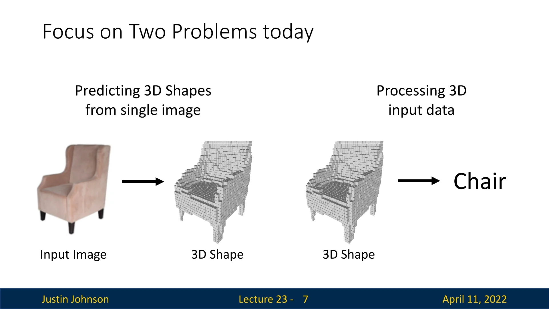
- 3D Shape Prediction: Given a single 2D image (e.g., of an armchair), the model predicts a corresponding 3D structure, such as a voxel grid that represents the shape of the object. This task is inherently ill-posed due to the loss of depth information in the 2D projection.
- 2.
- 3D-Based Classification: Given a 3D representation (e.g., a voxel grid), the model predicts the semantic class of the object (e.g., “armchair”), showing understanding from structural geometry.
Beyond these core problems, 3D vision encompasses a broad range of challenges such as motion estimation from depth, simultaneous localization and mapping (SLAM), multi-view reconstruction, and more. Importantly, due to the strong geometric structure of the 3D world, many classical vision algorithms (e.g., stereo triangulation) remain highly relevant and are often integrated with or benchmarked against learning-based methods.
23.1.2 3D Representations
A variety of representations can capture the geometry of 3D objects. While differing in format, all serve the common goal of describing shape and structure in three dimensions:
- Depth Map: A 2D grid where each pixel stores the distance (in meters) from the camera to the nearest surface point along the ray passing through that pixel. Captured by RGB-D sensors (e.g., Microsoft Kinect), these are often called 2.5D images since they only encode visible surfaces, not occluded regions.
- Voxel Grid: A 3D array of binary or real-valued occupancies representing whether a volume element (voxel) is occupied.
- Point Cloud: A sparse set of 3D points capturing surface geometry.
- Mesh: A polygonal surface composed of vertices, edges, and faces—typically used in graphics.
- Implicit Surface: A continuous function (e.g., signed distance function) where the zero-level set defines the surface of the object.
Despite differing computational properties and storage formats, all these representations aim to capture the same underlying 3D structure.
23.2 Predicting Depth Maps from RGB Images
One of the most accessible and widely studied 3D vision tasks is estimating a dense depth map from a single RGB image. This process, known as monocular depth estimation, aims to assign a depth value to each pixel, producing a 2.5D representation of scene geometry from a monocular input. The task is fundamentally ill-posed, as multiple 3D scenes can correspond to the same 2D projection, making monocular depth estimation a challenging problem that requires strong visual priors.
A common and effective architectural design for this task is the fully convolutional encoder-decoder network, which is well-suited to dense prediction tasks. These models process an input image through an encoder to extract semantically rich features and subsequently reconstruct a dense depth map via a decoder that upsamples these features to the input resolution. The fully convolutional nature of this pipeline ensures that the spatial correspondence between input pixels and output predictions is preserved, enabling pixel-aligned depth estimation.
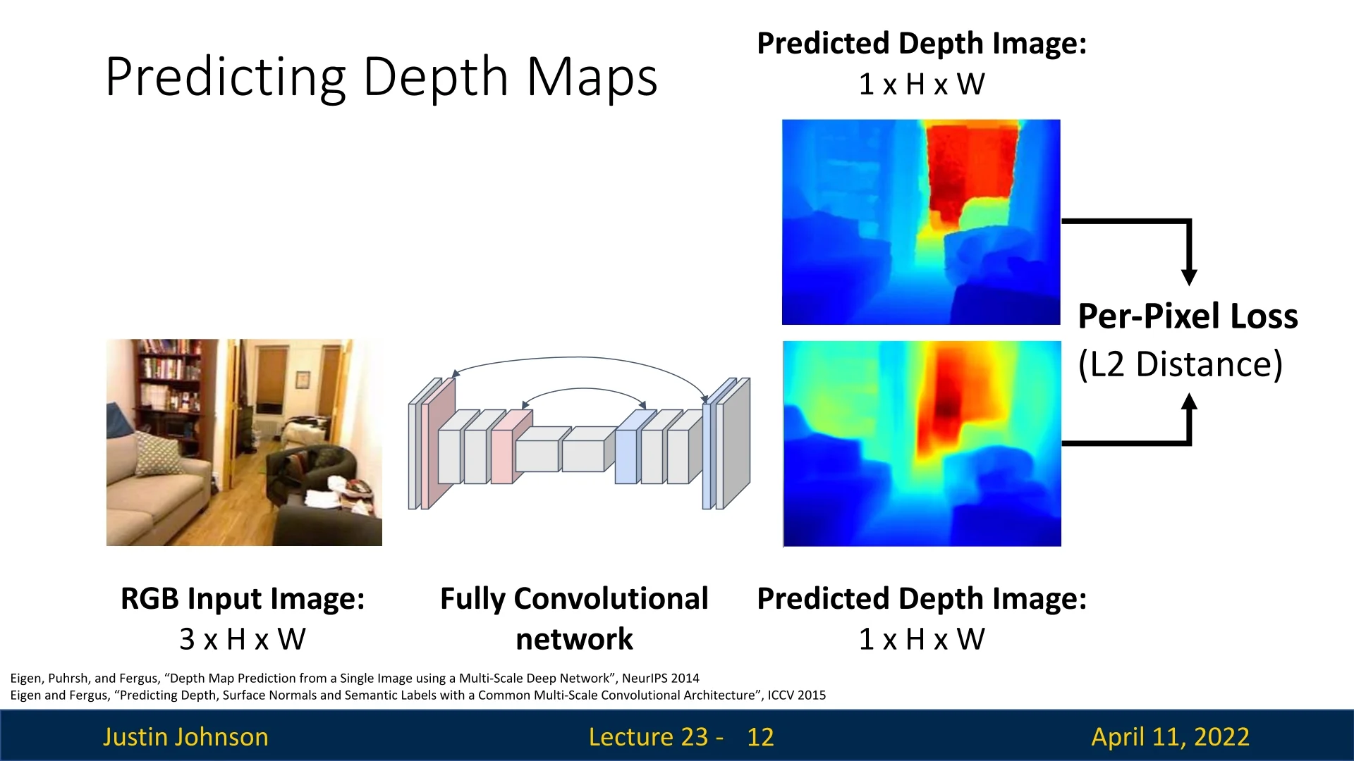
The encoder typically consists of a convolutional backbone (e.g., ResNet) pretrained on large-scale classification datasets like ImageNet. Through successive layers of strided convolutions, the encoder compresses the spatial resolution of the input while increasing the semantic abstraction and receptive field. This enables the network to aggregate both local texture and global scene layout, capturing information necessary for reasoning about object scale, occlusion, and perspective.
The decoder reverses this spatial compression, gradually upsampling the feature maps to predict a dense depth map. In U-Net-style architectures, skip connections are employed to concatenate feature maps from early encoder layers with corresponding decoder stages, facilitating the recovery of fine-grained details such as object boundaries and thin structures. This coarse-to-fine decoding strategy is particularly effective in reconciling global context with local spatial accuracy.
Several influential models build upon this framework:
- MiDaS [527] emphasizes generalization across diverse datasets. Later versions of MiDaS replace convolutional encoders with Vision Transformers (ViTs), leveraging global self-attention to capture long-range dependencies and scene-level structure. This shift enables more coherent depth maps, particularly in unfamiliar environments.
- BTS (From Big to Small) [329] enhances the decoder with local planar guidance (LPG) modules. These modules predict local plane parameters at multiple resolutions, guiding the reconstruction of depth maps by assuming piecewise planar geometry—a useful trait we can use for scenes with man-made structures or flat surfaces.
- DPT (Dense Prediction Transformer) [526] combines a ViT encoder with a convolutional decoder, explicitly designed for dense prediction tasks. DPT treats the image as a sequence of patches from the outset, enabling early global context aggregation. The decoder then reconstructs high-resolution outputs while retaining global consistency, resulting in state-of-the-art depth estimation performance on several benchmarks (at the time of publication).
While the architectural choices vary across models, the core principles remain consistent: extract semantically meaningful, globally aware features with the encoder; restore spatial detail and pixelwise correspondence with the decoder. These systems have made monocular depth estimation viable for real-time applications such as AR, robotics, and autonomous navigation, where dense 3D understanding from a single image is both efficient and essential.
Loss Function and the Limitations of Absolute Depth Regression A foundational approach to monocular depth estimation is to directly regress the ground truth depth using a pixel-wise \(\ell _2\) loss:
\[ \mathcal {L}_{\mbox{depth}} = \frac {1}{N} \sum _{i=1}^{N} \left ( d_i - \hat {d}_i \right )^2, \]
where \( d_i \) denotes the ground truth depth and \( \hat {d}_i \) is the predicted depth at pixel \( i \), for a total of \( N \) pixels. This objective treats depth estimation as a supervised regression task, optimizing the per-pixel distance between prediction and annotation.
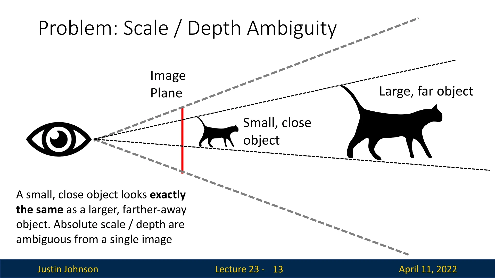
Scale-Depth Ambiguity and the Need for Invariant Losses Despite its simplicity, the \(\ell _2\) loss fails to account for a fundamental limitation in monocular depth estimation: scale-depth ambiguity. Given only a single RGB image, there exist infinitely many 3D scenes that could yield the same 2D projection. For example, a small object placed close to the camera may appear identical in the image to a larger object situated farther away. This ambiguity makes the estimation of absolute scale from monocular input fundamentally ill-posed.
While cues such as object size priors, vanishing points, or scene layout may offer some information, the absolute scale remains ambiguous without auxiliary data. Consequently, modern methods replace or augment the naïve \(\ell _2\) objective with loss functions that are invariant to scale and shift and that emphasize relative structure.
Scale-Invariant Log-Depth Loss Monocular depth estimation suffers from scale-depth ambiguity: an image alone does not reveal whether a small object is nearby or a large object is far away. This ambiguity renders absolute depth supervision fundamentally ill-posed without geometric cues. To address this, [142] proposed a scale-invariant loss that focuses on preserving relative scene structure while remaining agnostic to global depth scale.
Let \( \hat {d}_i \) and \( d_i \) denote the predicted and ground truth depth at pixel \( i \), respectively. Define the log-space residual at each pixel as \[ \delta _i = \log \hat {d}_i - \log d_i = \log \left ( \frac {\hat {d}_i}{d_i} \right ). \] This transforms multiplicative depth errors—such as those caused by an overall scaling mistake—into additive biases in log space. For example, if all predictions are off by a constant factor \( s \), then \( \delta _i = \log s \) for all \( i \).
The scale-invariant loss is given by: \[ \mathcal {L}_{\mbox{SI}} = \frac {1}{n} \sum _{i=1}^n \delta _i^2 - \frac {1}{n^2} \left ( \sum _{i=1}^n \delta _i \right )^2. \] The first term penalizes pixelwise errors in log-depth, while the second term subtracts the squared mean residual. This centering step ensures that uniform log-space errors—i.e., global scaling shifts—do not contribute to the loss. In the case where \( \hat {d}_i = s \cdot d_i \) for all \( i \), we have \( \delta _i = \log s \) and the two terms cancel exactly, yielding zero loss.
Pairwise Interpretation An equivalent expression of the same loss emphasizes its structural nature: \[ \mathcal {L}_{\mbox{SI}} = \frac {1}{n^2} \sum _{i,j} \left [ \left ( \log \hat {d}_i - \log \hat {d}_j \right ) - \left ( \log d_i - \log d_j \right ) \right ]^2. \] Here, the loss is computed over all pixel pairs, enforcing that the difference in predicted log-depth between any two pixels matches the difference in ground truth log-depth. This pairwise comparison naturally preserves the relative depth ordering and ratios across the image, which define the 3D scene structure up to scale.
Weighted Loss for Training In practice, [142] used a weighted variant of the loss to trade off scale sensitivity and structure preservation. The training objective is: \[ \mathcal {L}_{\mbox{train}} = \frac {1}{n} \sum _i \delta _i^2 - \lambda \cdot \frac {1}{n^2} \left ( \sum _i \delta _i \right )^2, \] where \( \lambda \in [0,1] \) determines how strongly the loss penalizes global scale errors. Setting \( \lambda = 0 \) recovers the standard log-MSE, while \( \lambda = 1 \) gives the fully scale-invariant loss. The authors found \( \lambda = 0.5 \) to offer a good balance—preserving global scale roughly while improving structural coherence and visual quality of the depth maps.
Why a Single Global Scale Correction Suffices Monocular images lack metric information, so networks often make consistent global depth errors—predicting all depths as uniformly too large or too small. This happens because, without geometric supervision, the model can recover scene structure (e.g., which objects are closer) but not absolute scale.
Importantly, such scale errors are not local: the network does not typically stretch some parts of the scene while shrinking others. Instead, the entire scene is scaled by a single factor \( s \), yielding predictions \( \hat {d}_i = s \cdot d_i \) for all pixels \( i \). For instance, if a model interprets a real cat as a small nearby toy, it will likely interpret a real car as a small toy car—misestimating scale consistently across objects and spatial regions.
This uniformity arises because the only available supervision—the ground truth depth—reveals the correct scale globally. Thus, if the network makes a pure scaling mistake, it will affect all depths equally, and a single correction factor suffices to align prediction with ground truth: \[ \frac {\hat {d}_i}{\hat {d}_j} = \frac {s \cdot d_i}{s \cdot d_j} = \frac {d_i}{d_j}. \] The scale-invariant loss captures this by canceling out any constant log-depth offset across the image. It ensures the network is trained to preserve relative structure, while ignoring inevitable global scale ambiguity in monocular input.
Scale and Shift-Invariant Losses in MiDaS and DPT Training monocular depth models on diverse datasets poses a core challenge: different datasets often encode depth with varying units, unknown camera baselines, or arbitrary scale and shift. For example, structure-from-motion yields depths up to scale, while stereo systems may produce disparities with dataset-specific offsets. Comparing predictions directly to such ground truth is ill-defined.
To address this, MiDaS [527] and DPT [526] adopt a scale and shift invariant objective that aligns predictions to ground truth before measuring error. Specifically, they operate in inverse depth (disparity) space—numerically stable and compatible with diverse sources—and fit an affine transformation to the predicted disparity \( \hat {d} \in \mathbb {R}^N \) to match the ground truth \( d \in \mathbb {R}^N \). The aligned prediction is given by: \[ \hat {d}_{\mbox{aligned}} = a \hat {d} + b, \] where \( a \in \mathbb {R} \) (scale) and \( b \in \mathbb {R} \) (shift) are computed via closed-form least-squares.
Robust Trimmed MAE and Multi-Scale Gradient Losses Once aligned, the model minimizes two complementary objectives that address distinct challenges in real-world training data:
1. Trimmed Mean Absolute Error (tMAE). Rather than computing loss over all pixels, MiDaS and DPT discard the highest residuals—typically the top 20%—and compute the L1 error over the remaining high-confidence set \( \mathcal {I} \subset \{1, \dots , N\} \): \[ \mathcal {L}_{\mbox{tMAE}}(d, \hat {d}) = \frac {1}{|\mathcal {I}|} \sum _{i \in \mathcal {I}} \left | a \hat {d}_i + b - d_i \right |. \]
This trimmed loss improves robustness in two ways. First, the use of L1 error prevents extreme residuals from dominating the loss—unlike L2, which excessively penalizes large errors. Second, trimming ensures that corrupted or misaligned pixels (e.g., due to missing depth, motion blur, or sensor artifacts) do not influence training. In effect, it converts noisy datasets into reliable training signals by emphasizing clean, consistent regions first, and gradually incorporating harder cases as the model improves.
2. Multi-Scale Gradient Matching. While the trimmed MAE loss ensures accuracy on reliable pixels, it does not capture how depth changes across space—that is, it ignores the local geometry of surfaces. To remedy this, MiDaS and DPT incorporate a multi-scale gradient loss that encourages the predicted depth map to exhibit the same structural transitions and surface boundaries as the ground truth.
The depth gradient at a pixel refers to the rate of change in depth with respect to its horizontal and vertical neighbors. In flat, smooth regions (e.g., walls, floors), depth changes slowly and the gradient is small. At object boundaries or depth discontinuities (e.g., the edge of a chair or the silhouette of a person), depth shifts abruptly and the gradient is large. Thus, gradients serve as a proxy for geometry: they capture where and how the scene bends, steps, or ends.
Mathematically, the spatial gradient \( \nabla d_i \) is computed using finite differences in the \(x\) and \(y\) directions—typically as: \[ \nabla d_i = \left ( d_{i+\hat {x}} - d_i,\;\; d_{i+\hat {y}} - d_i \right ), \] where \( \hat {x} \) and \( \hat {y} \) denote offsets to right and bottom neighbors. This simple local operation reveals the slope of the depth surface around each pixel.
The multi-scale gradient loss compares these gradients between prediction and ground truth at various spatial resolutions: \[ \mathcal {L}_{\mbox{grad}} = \sum _{s} \frac {1}{N_s} \sum _{i=1}^{N_s} \left \| \nabla \hat {d}_i^{(s)} - \nabla d_i^{(s)} \right \|_1. \] The use of an L1 norm ensures robustness to local mismatches. The summation over scales \( s \) (e.g., full, half, quarter resolution) allows the model to reason about both coarse structure (e.g., floor-to-wall transitions) and fine details (e.g., edges of thin objects).
Why it works: Traditional pixel-wise losses tend to average out sharp transitions, producing overly smooth or blurry depth maps. Gradient supervision counteracts this by explicitly penalizing structural mismatches. It teaches the model not only to match depth values, but to replicate the contours and discontinuities that define the geometry of the scene.
In effect, this loss forces the network to answer: Where do depth changes occur? How sharply? Do they match real-world object boundaries? The result is depth predictions with sharper edges, more accurate occlusions, and higher geometric fidelity—particularly important in zero-shot transfer settings where structure is more reliable than absolute scale.
Summary While pixel-wise \(\ell _2\) loss offers a straightforward entry point to monocular depth estimation, it fails to resolve the ill-posed nature of global scale recovery. Modern approaches instead adopt scale- and shift-invariant losses in log-depth or inverse-depth space, often augmented with gradient structure terms. These advances—combined with diverse training data and stronger architectures—have led to state-of-the-art results in monocular depth estimation across benchmarks such as KITTI, NYUv2, and ETH3D.
23.3 Surface Normals as a 3D Representation
In addition to depth maps, another powerful per-pixel 3D representation is that of surface normals. For each pixel in the input image, the goal is to estimate a 3D unit vector that represents the orientation of the local surface at that point in the scene. Surface normals are tightly linked to the underlying geometry of the object and provide a complementary view to depth.
Unlike depth, which encodes the distance between the camera and scene points, surface normals capture orientation, offering critical cues for understanding shape, curvature, and object boundaries.
Visualizing Normals Since each surface normal is a unit vector in \(\mathbb {R}^3\), they can be visualized as RGB images by mapping the \(x\), \(y\), and \(z\) components of each normal vector to the red, green, and blue color channels, respectively. This visualization provides intuitive insight into the orientation of different surfaces.
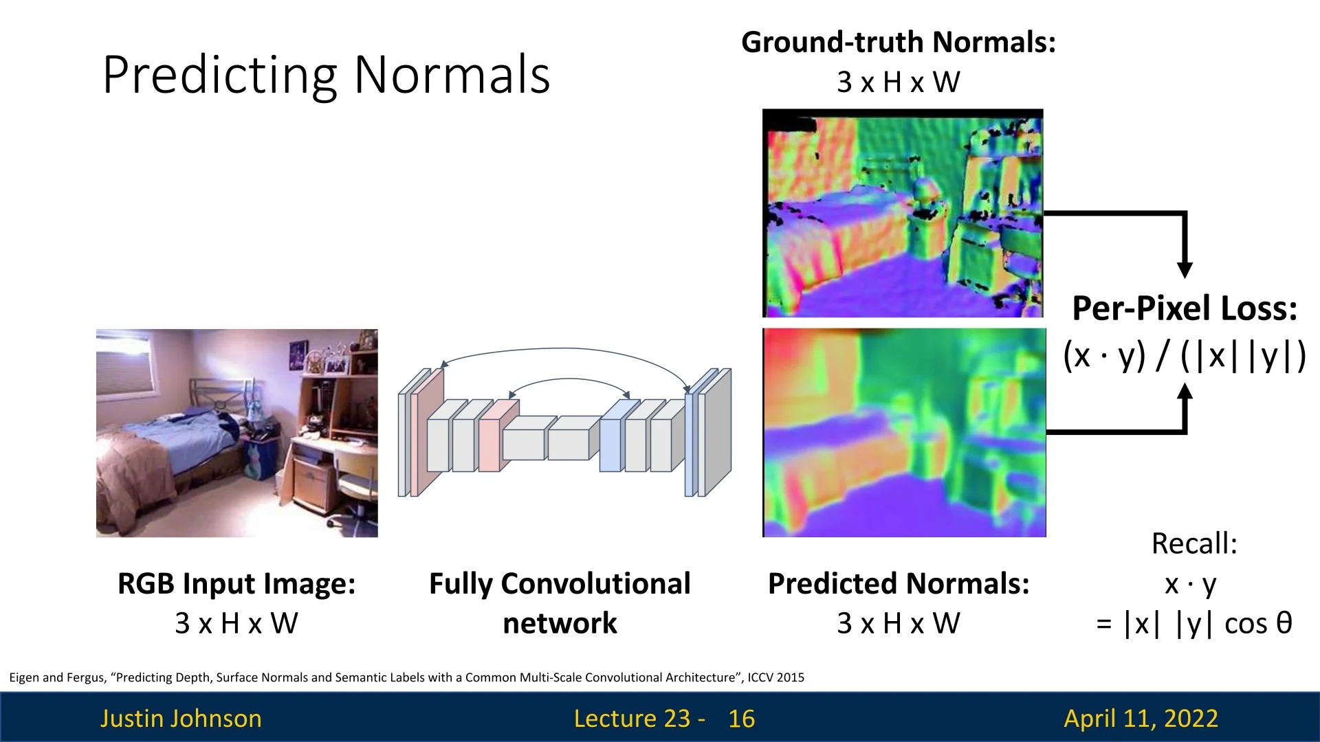
Learning Surface Normals Similar to depth prediction, surface normal estimation can be framed as a dense regression task using a fully convolutional network. The network predicts a unit vector \( \hat {\mathbf {n}}_i \in \mathbb {R}^3 \) for each pixel \( i \), and the objective is to align it with the corresponding ground truth normal \( \mathbf {n}_i \in \mathbb {R}^3 \). Since the predicted and ground truth vectors should have the same direction regardless of scale, a natural loss function is the cosine similarity loss:
\[ \mathcal {L}_{\mbox{normal}} = \frac {1}{N} \sum _{i=1}^{N} \left ( 1 - \frac { \hat {\mathbf {n}}_i \cdot \mathbf {n}_i }{ \| \hat {\mathbf {n}}_i \|_2 \cdot \| \mathbf {n}_i \|_2 } \right ), \]
where \( \cdot \) denotes the dot product and \( \| \cdot \|_2 \) is the Euclidean norm. Note that since ground truth normals are unit vectors, predicted vectors are often explicitly normalized before loss computation.
Multi-Task Learning In practice, tasks like dense segmentation and surface normal prediction are often trained jointly in a multi-task setup, sharing the same encoder but having separate decoders. This setup encourages the model to learn a richer and more consistent geometric understanding of the scene.
Limitations While both depth and surface normals provide dense and informative representations of the visible geometry in an image, they share a critical limitation: they are inherently restricted to visible surfaces. Occluded regions, hidden backsides, and self-occlusions are not represented, leading to incomplete scene understanding. To address this, more global 3D representations such as voxels, point clouds, or meshes are necessary, as they model complete volumetric structure beyond the image plane.
23.4 Voxel Grids
To model 3D geometry beyond visible surfaces, one of the most intuitive volumetric representations is the voxel grid. A voxel grid discretizes 3D space into a cubic lattice of resolution \( V \times V \times V \), where each voxel encodes occupancy information—typically as a binary value: \(1\) if the voxel is occupied by an object, and \(0\) otherwise. This can be viewed as the 3D analog of a 2D binary segmentation mask, but extended to volumetric space.
Voxel grids offer a conceptually simple and regular structure, making them attractive for early 3D learning pipelines. The representation is reminiscent of how objects are composed in voxel-based environments such as Minecraft, where entire scenes are built from discrete blocks.
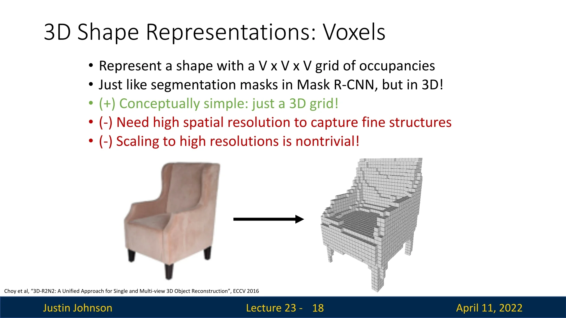
Advantages The voxel grid format enables straightforward adaptation of classical CNN-based architectures to 3D data by replacing 2D convolutions with 3D convolutions. Since the voxel grid is regular and aligned to a grid structure, operations like pooling, upsampling, and convolution generalize naturally from 2D to 3D.
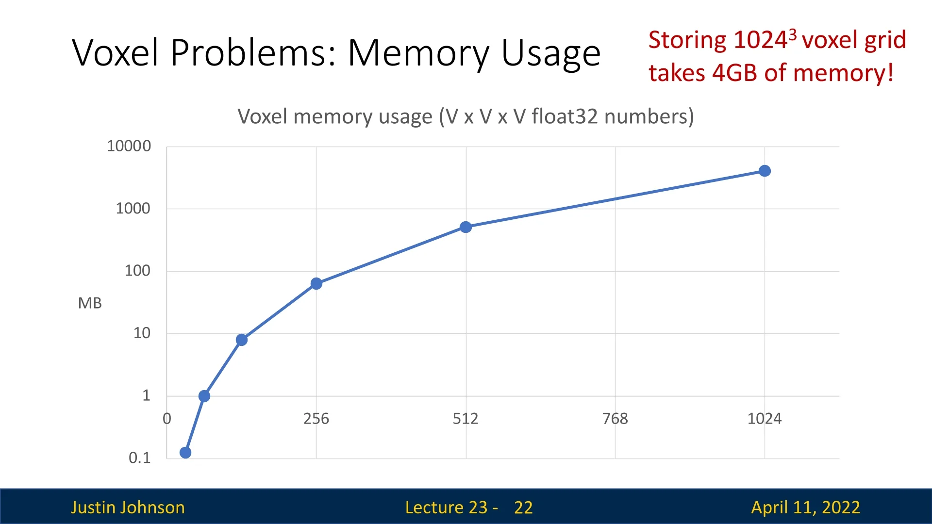
Limitations A critical downside of voxel-based representations is their poor scalability with resolution. The memory and computational cost of processing a voxel grid scales cubically with resolution: storing a grid of resolution \( V \) requires \( O(V^3) \) space. This rapidly becomes intractable for high-resolution scenes or objects, and fine details are lost at coarse voxel resolutions.
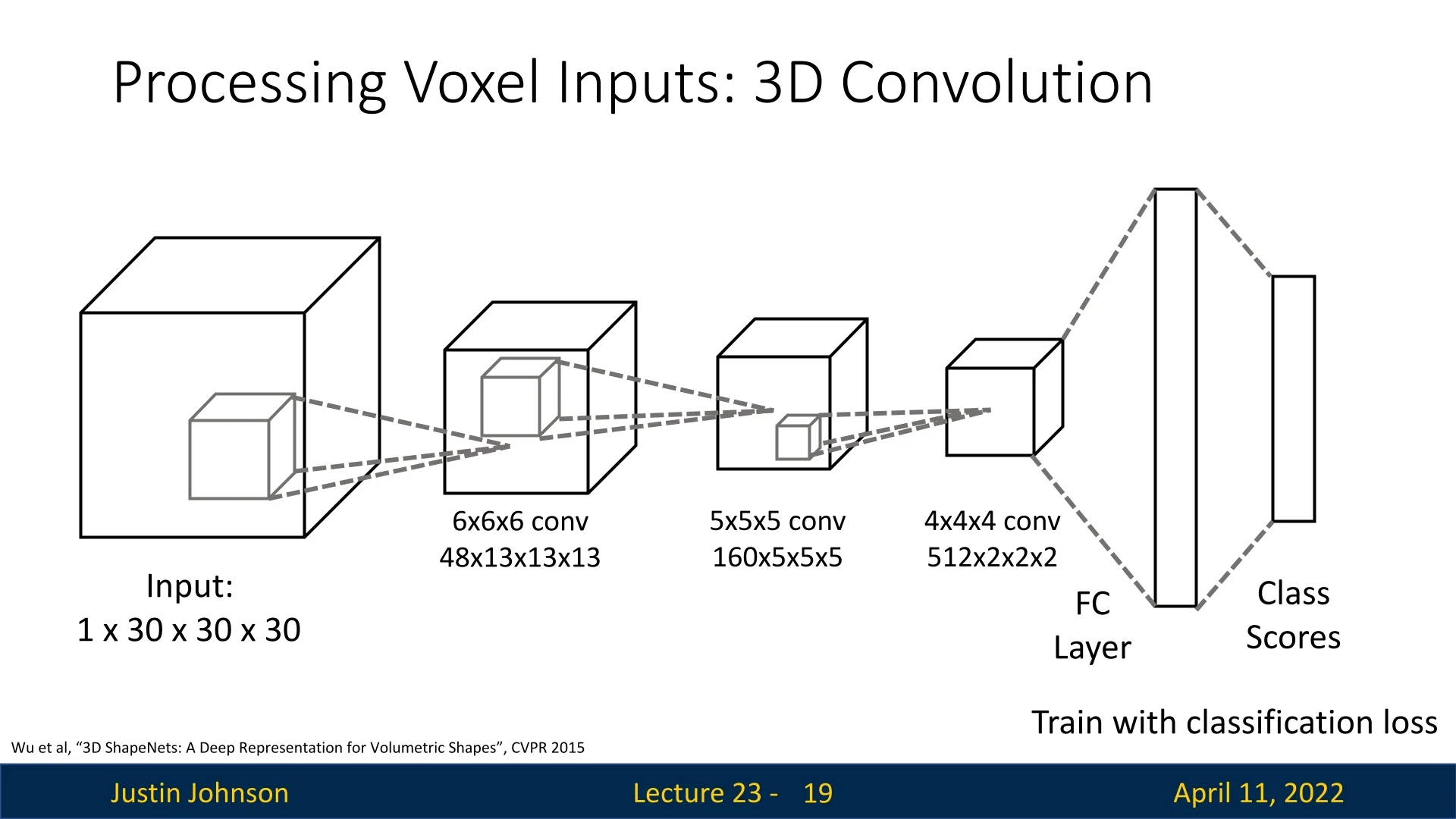
3D Convolutional Processing Similar to 2D convolution, a 3D convolution applies a local filter over spatial neighborhoods in the voxel grid. The kernel is a 3D volume of shape \( k \times k \times k \) (typically \(k=3\) or \(5\)), and it slides across the grid to compute local features:
\[ y(i, j, k) = \sum _{u,v,w} x(i+u, j+v, k+w) \cdot w(u, v, w), \]
where \( x \) is the input voxel grid or feature map, \( w \) is the learned 3D kernel, and \( y \) is the resulting activation map. These operations can be stacked in deep 3D convolutional networks to perform classification, segmentation, or shape completion.
Application Example: Image-to-Voxel Prediction A representative application of voxel-based shape representation is 3D reconstruction from a single RGB image. In this example, an image of an armchair is processed by a 2D convolutional neural network to extract high-level visual features. These features are then projected into a latent 3D space and refined through a sequence of 3D convolutional layers, ultimately producing a predicted voxel occupancy grid.
The pipeline begins with a \(3 \times 112 \times 112\) input image, which is passed through a 2D CNN backbone to generate a compressed feature representation. This feature tensor is reshaped or lifted into a 3D voxel grid of shape \(1 \times V \times V \times V\) (e.g., \(32^3\)). The lifted volume is then processed by 3D convolutional filters that reason about the spatial structure of the object in three dimensions.
The final output is a binary or probabilistic voxel grid indicating which regions of 3D space are likely to be occupied by the object. In our example, the network successfully reconstructs the volumetric shape of an armchair directly from a single view.
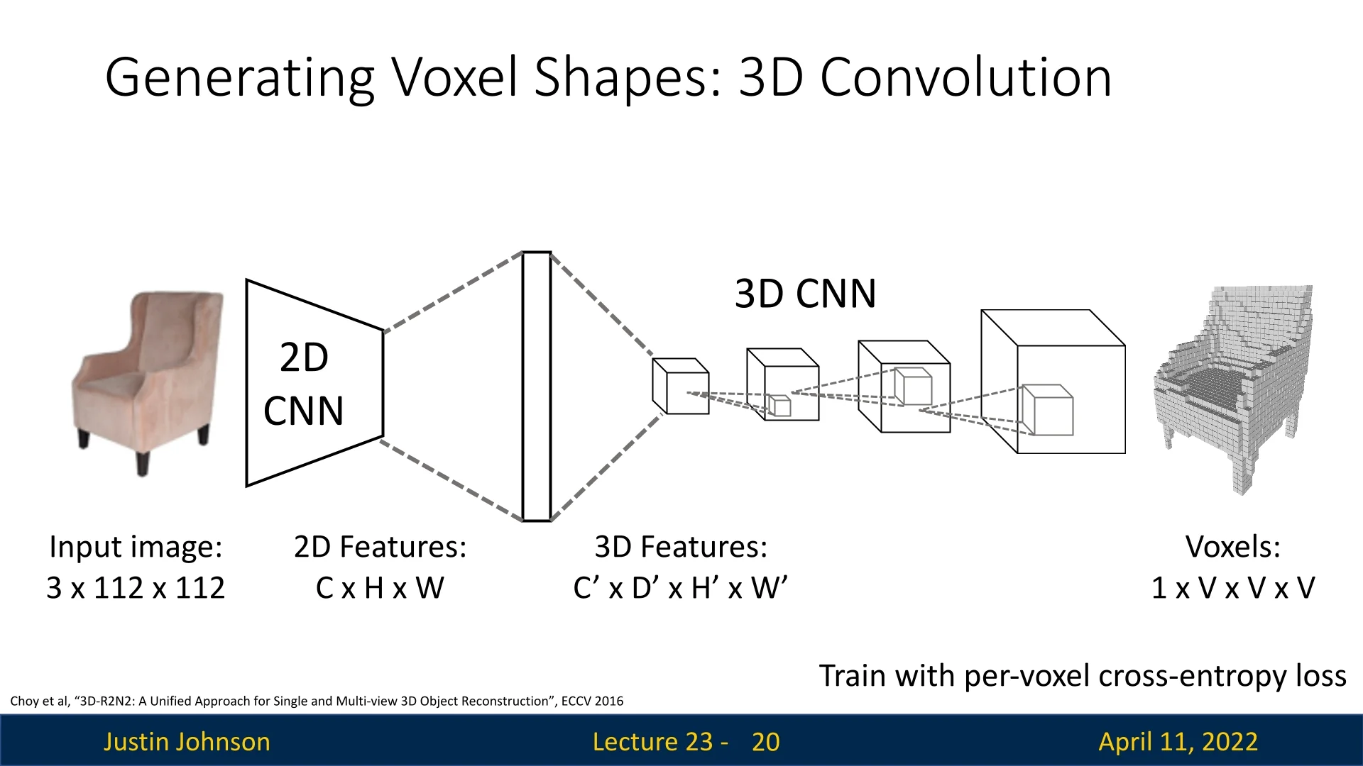
This architecture exemplifies how convolutional models can bridge 2D visual perception and 3D spatial reasoning. The voxel grid serves as an interpretable intermediate representation, enabling volumetric reasoning for tasks such as shape completion, reconstruction, etc.
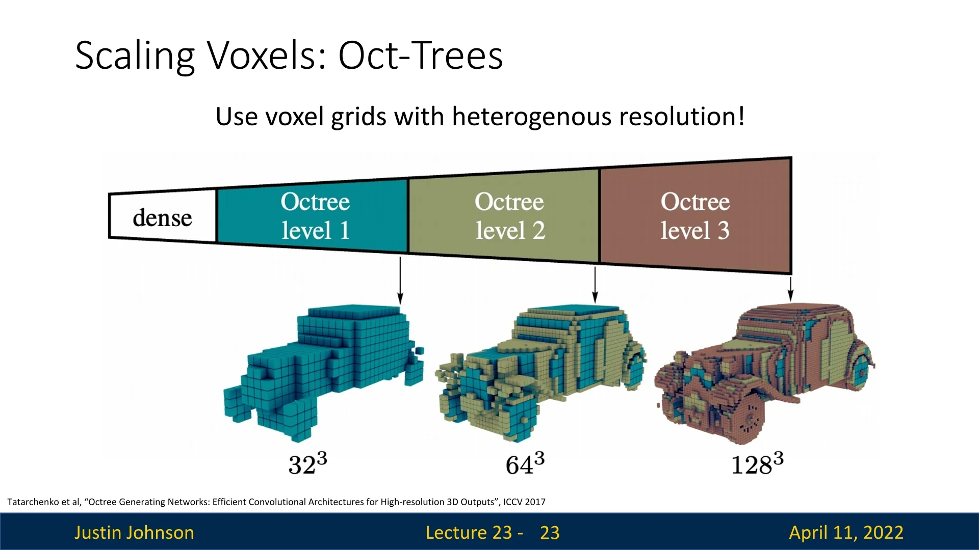
As can be seen in figure 23.8, due to the cubic growth of memory and compute with resolution, voxel-based methods are constrained in practice, motivating alternative representations such as point clouds, triangle meshes, and neural implicit fields for higher-fidelity modeling. One thing we can do though, is try to scale voxels based on Oct-Trees.
23.4.1 Scaling Voxel Grids with Octrees
Standard voxel grids suffer from a key limitation: memory and computation grow cubically with resolution. For instance, going from a \(32^3\) to \(128^3\) grid multiplies storage cost by a factor of \(4^3 = 64\). At high resolutions, this becomes intractable—even though most of the grid is typically empty or homogeneous. This makes dense voxelization wasteful and limits its ability to capture fine geometric detail.
To overcome this inefficiency, Tatarchenko et al. introduced the Octree Generating Network (OGN) [629], which replaces dense grids with a sparse hierarchical structure called an octree.
Octrees: Intuition and Structure An octree is a tree-based representation that adaptively subdivides 3D space. Starting from a single cube that covers the full scene (the root), each cube is recursively split into eight subcubes (octants)—but only when that region contains surface detail. Empty or homogeneous regions remain unrefined.
- Uniform regions (e.g., open air or flat walls) are stored as large, coarse octree nodes.
- Detailed regions (e.g., object boundaries or thin parts) are recursively subdivided to finer scales.
This adaptive spatial resolution means memory is focused where it matters: on the surface.
From Dense to Adaptive To illustrate the impact, consider representing a car at different voxel resolutions:
- A dense \(128^3\) grid would allocate over two million voxels, even for empty space.
- In contrast, an octree might use only thousands of voxels—concentrated near the car’s surface.
This reduces overall memory complexity from \(O(n^3)\) to approximately \(O(n^2)\), since the object’s surface is a 2D manifold embedded in 3D space.
Octree Generating Networks (OGNs) OGN is a convolutional architecture that generates high-resolution 3D shapes in octree format. It starts with a coarse prediction of shape (e.g., \(8^3\) or \(16^3\)) and recursively refines it. The model learns to predict:
- which voxels should be subdivided (occupancy probabilities),
- and what features to pass to each child octant (learned latent codes).
At each refinement level, the network only expands voxels flagged as informative. This enables high-fidelity 3D shape generation—without wasting memory on empty regions.
Surface-Driven Efficiency The advantage of octrees becomes clearest at high resolutions. Rather than processing millions of voxels uniformly, OGNs focus computation where object geometry is complex. For example, flat car doors are left coarse, while wheels or window edges are subdivided further.
Why and How Octrees Work Octrees address storage inefficiency by adaptively refining the voxel grid only where necessary, enabling surface-focused representations with far less memory.
How it works: The octree starts with a coarse resolution (e.g., \(32^3\)) and maintains a tree where each node represents a voxel. Each node can be classified as:
- empty: the voxel contains no surface and is not refined further;
- filled: the voxel lies entirely inside the object and needs no further subdivision;
- mixed: the voxel intersects a surface and is therefore recursively subdivided into 8 children.
The key challenge is determining which voxels to refine.
Predicting Subdivision with Neural Networks At each level of refinement, the octree maintains a sparse set of active leaf voxels. For each such voxel, the network predicts:
- 1.
- A feature vector for the current voxel (using sparse 3D convolutions on the octree structure).
- 2.
- An occupancy classification score for the voxel itself.
- 3.
- A set of 8 binary flags, one for each potential child voxel. indicating whether that subregion should be refined.
The voxel is only subdivided if at least one child is predicted as filled or mixed—that is, likely to be part of the object’s interior or intersect the surface. These predictions are made using a split prediction head that branches off the decoder.
Training with Supervised Supervision OGNs are trained end-to-end using ground truth voxel occupancy grids, from datasets like ShapeNet. The training process proceeds in a coarse-to-fine manner:
- At level \(l\) (e.g., \(32^3\)): The network processes the current octree level and predicts occupancy and subdivision flags for each voxel.
- Ground truth comparison: The predicted occupancy labels and subdivision decisions are supervised using binary cross-entropy losses against a precomputed ground truth octree. These labels are derived by voxelizing the 3D CAD mesh and marking voxels as filled, empty, or mixed.
- Subsequent levels: Only voxels marked for refinement are subdivided. Their children become the active set for the next finer resolution level (e.g., \(64^3\), then \(128^3\), etc.).
This recursive supervision continues until the desired maximum resolution is reached. The result is a hierarchical, sparsely populated voxel grid that concentrates resolution along object surfaces, drastically reducing memory and computation.
- Focuses computation: By refining only ambiguous voxels, the model avoids spending resources on empty space or flat interiors.
- Learns detail adaptively: The network learns where detail is needed from data, rather than relying on hand-crafted refinement rules.
- Enables higher resolutions: Because only a subset of voxels are represented at each level, OGNs can generate outputs at resolutions like \(256^3\) or \(512^3\) with the memory footprint of a much smaller dense grid.
This learned coarse-to-fine generation strategy allows octree-based models to efficiently capture complex geometry while remaining scalable, making them highly effective for high-resolution 3D shape prediction tasks.
Limitations and Motivation for Point-Based Methods Despite their efficiency, octrees still discretize space into axis-aligned cubes, which limits their ability to model very fine surface curvature or sharp boundaries without deep subdivisions. Moreover, generating and traversing octree hierarchies can introduce implementation complexity and latency in practice.
These limitations motivate an alternative family of 3D representations: point clouds. Unlike voxel grids or octrees, point clouds represent surfaces directly via sampled points in \(\mathbb {R}^3\), bypassing the need to discretize space altogether. Although voxel representation is pretty common in practice, and point-based methods do not benefit from the grid structure useful in convolutional networks, they are intriguing as they offer greater flexibility and memory efficiency, especially for capturing fine-grained surface geometry.
In the following part, we explore point cloud representations and the neural architectures designed to process them effectively.
23.5 Point Clouds
A point cloud is a flexible, sparse, and surface-centric representation of 3D geometry. It models an object as a set of \( P \) points in \( \mathbb {R}^3 \), each corresponding to a sampled position on the visible surface: \[ \mathcal {P} = \{ \mathbf {p}_i \in \mathbb {R}^3 \mid i = 1, \ldots , P \} \]
Unlike voxel grids, which discretize the 3D space uniformly and incur cubic memory costs, point clouds only represent surface points, yielding a compact and efficient encoding. This representation aligns naturally with real-world sensor data, such as LiDAR in autonomous vehicles.
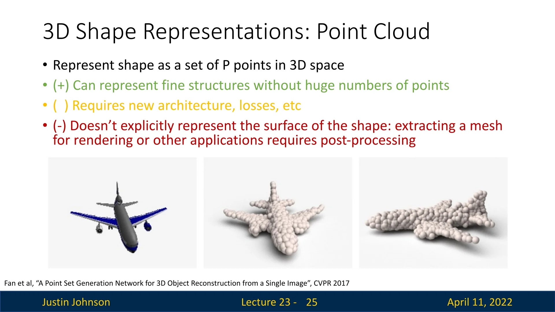
Advantages Point clouds allow for high-resolution geometric modeling without the cubic scaling of voxel-based methods. They efficiently capture fine details such as airplane wings or chair slats using a relatively small number of points (as shown in figure 23.10), while coarser regions like planar surfaces can be represented sparsely.
Limitations Point clouds do not encode surface connectivity or topology. This limits their utility for downstream applications such as mesh rendering or physics simulation, which rely on explicit surface structure. Additionally, point clouds are unordered and irregularly sampled, requiring specialized neural architectures for effective processing.
Rendering Since mathematical points are infinitesimal, visualizations inflate each point into a finite-radius sphere. This creates the illusion of a continuous surface but does not resolve the lack of connectivity. To use point clouds for graphics or simulation, surface reconstruction via meshing algorithms is often necessary.
Applications Point clouds are a core representation in 3D perception and are widely used in robotics, AR/VR, and autonomous driving. In particular, LiDAR sensors deployed on self-driving vehicles emit laser pulses to scan the environment and return a dense set of 3D points corresponding to surfaces in the scene. This raw point cloud data forms the foundation for several high-level tasks:
- Obstacle detection and tracking: Dynamic objects such as vehicles, pedestrians, and cyclists are localized and tracked in 3D space, enabling collision avoidance and motion planning.
- Semantic scene understanding: Each point in the cloud can be semantically labeled as road, building, vegetation, etc., supporting downstream reasoning about the environment.
- Mapping and localization: Aggregated LiDAR scans are used to construct high-definition (HD) maps for accurate self-localization and route planning. These maps include fine-grained structures such as lane boundaries, curbs, and traffic signs.
- Multi-sensor fusion: Point clouds are often fused with camera and radar inputs to improve robustness under challenging conditions, such as poor lighting or weather, where single modalities may fail.
By capturing precise geometric structure independent of appearance, point clouds enable spatial reasoning and metric-scale perception, making them indispensable for autonomous systems operating in complex, dynamic environments.
23.5.1 Point Cloud Generation from a Single Image
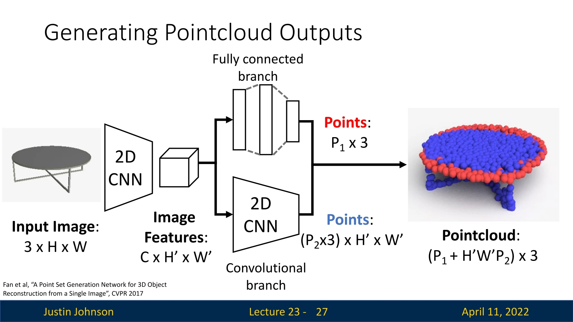
Fan et al. [153] introduce a landmark framework for reconstructing 3D shapes as point sets directly from a single RGB image. Unlike voxel grids or multi-view representations, point clouds are efficient, resolution-independent, and naturally suited to surface-level geometry. The model predicts an unordered set of 3D points \[ \hat {S} = \{\,\hat {y}_i\,\}_{i=1}^{P_1 + H'W'P_2} \subset \mathbb {R}^3, \] which approximates the visible object surface.
Architecture Overview The model follows an encoder–decoder structure with a dual-branch output head designed to capture both global object structure and fine surface detail.
- The encoder is a convolutional neural network that maps the input image \( I \in \mathbb {R}^{3 \times H \times W} \) to a latent feature tensor \( F \in \mathbb {R}^{C \times H' \times W'} \). This feature map encodes rich spatial information about the input’s underlying 3D geometry.
-
The decoder splits into two complementary branches:
-
Fully-Connected (Global) Branch: The feature map \(F\) is flattened and passed through a multi-layer perceptron (MLP) to produce a fixed set of \(P_1\) 3D points: \[ \hat {S}^{\mathrm {g}} = \{\,\hat {y}_i^{\mathrm {g}}\,\}_{i=1}^{P_1} \subset \mathbb {R}^3. \] The output dimensionality is predetermined—e.g., a final layer with \(3 \cdot P_1\) units reshaped into a \(P_1 \times 3\) matrix. This branch captures the global structure, pose, and coarse silhouette of the object. The hyperparameter \(P_1\) is typically chosen to balance expressiveness and efficiency, and remains fixed during training and inference.
- Convolutional (Local) Branch: Rather than collapsing spatial dimensions, this branch operates directly over the \(H' \times W'\) grid of the encoded feature map. At each spatial location \((i, j)\), a shared MLP (implemented as \(1 \times 1\) convolution) predicts \(P_2\) 3D points: \[ \hat {S}^{\mathrm {l}} = \{\,\hat {y}_{i,j,k}^{\mathrm {l}}\,\}_{i=1}^{H'}{}_{j=1}^{W'}{}_{k=1}^{P_2} \subset \mathbb {R}^3. \] Each point is generated relative to a canonical 2D grid anchor, allowing the network to model high-frequency surface detail. The weight-sharing mechanism enforces translation-equivariant behavior across the image, which is particularly effective for capturing fine geometry such as edges, contours, and thin structures. Because it preserves spatial layout, this branch provides dense, localized surface coverage.
-
The final output is the union of both branches: \[ \hat {S} = \hat {S}^{\mathrm {g}} \cup \hat {S}^{\mathrm {l}}, \quad \mbox{with} \quad |\hat {S}| = P_1 + H'W'P_2. \]
This architecture enables the model to combine a globally consistent shape prior (via the FC branch) with spatially grounded local refinement (via the convolutional branch), yielding geometrically faithful point cloud reconstructions with efficient capacity allocation.
Architectural Motivation This dual-path architecture reflects a coarse-to-fine design philosophy:
- The global branch supplies a stable structural prior, capturing the object’s pose, orientation, and rough geometry.
- The local branch attends to spatially localized visual cues, enriching the surface detail with high-frequency geometric structure—particularly beneficial for recovering thin parts and sharp edges.
Together, they allow the network to generate accurate and detailed 3D reconstructions while keeping output size and model complexity manageable.
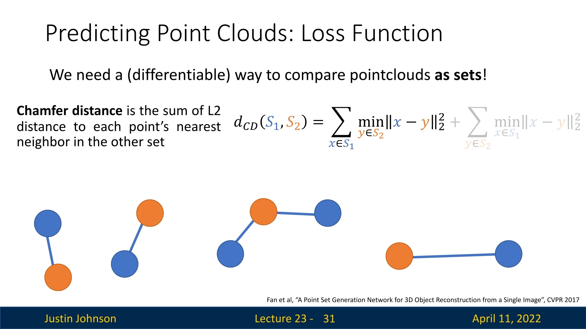
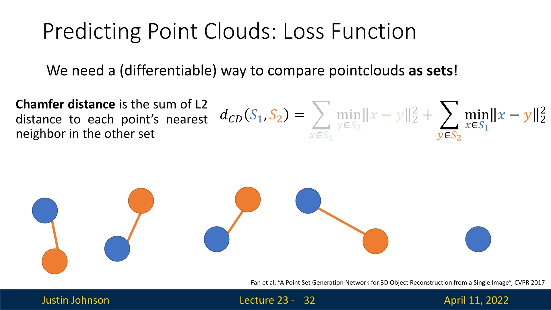
Loss Function: Chamfer Distance When predicting 3D point clouds, we aim to generate a set of points that matches a ground-truth shape surface. Crucially, both the predicted and target sets are unordered—permuting point indices does not change the represented shape. This calls for a set-based loss function that is invariant to point ordering and flexible to varying cardinality.
Fan et al. address this with the Chamfer Distance (CD), a symmetric, differentiable measure of dissimilarity between two point sets:
- \( S_1 \subset \mathbb {R}^3 \): predicted point cloud (previously \( \hat {S} \))
- \( S_2 \subset \mathbb {R}^3 \): ground-truth point cloud (previously \( S \))
The Chamfer Distance is defined as: \[ d_{\mathrm {CD}}(\textcolor {blue}{S_1}, \textcolor {orange}{S_2}) = \sum _{\textcolor {blue}{x \in S_1}} \min _{\textcolor {orange}{y \in S_2}} \|x - y\|_2^2 + \sum _{\textcolor {orange}{y \in S_2}} \min _{\textcolor {blue}{x \in S_1}} \|x - y\|_2^2. \]
Each term plays a complementary role:
- The forward term ensures that every predicted point \( \textcolor {blue}{x \in S_1} \) has a close match in the target set \( \textcolor {orange}{S_2} \). This promotes accurate surface fitting and penalizes extraneous predictions.
- The backward term guarantees that every target point \( \textcolor {orange}{y \in S_2} \) is approximated by at least one predicted point \( \textcolor {blue}{x \in S_1} \). This ensures full coverage of the ground-truth surface, even when the model predicts fewer points than the reference.
The bidirectional structure is key: even if \( |S_1| \neq |S_2| \), the loss still compares them fairly by asking how well each set ”explains” the other through nearest-neighbor matching. The use of minimum distances makes the loss permutation-invariant, and its differentiability (almost everywhere) enables end-to-end gradient-based optimization. Efficient computation is facilitated via KD-trees or approximate nearest neighbor search. The only situation in which the loss will be 0 is when the two sets are the same (each point in one is exactly on a point in the other), which is what we wanted to achieve.
Intuition and Impact The Chamfer Distance aligns naturally with the set-based nature of point clouds. By evaluating how well two sets approximate each other through nearest neighbors, it handles variable point counts and spatial distributions with ease. This makes it ideal for training neural networks to generate dense 3D surfaces from sparse supervision. Fan et al.’s use of Chamfer loss, coupled with a dual-branch decoder and CNN encoder, marked the first end-to-end framework to lift 2D images into 3D point sets with high geometric fidelity—laying the groundwork for many subsequent advances in point-based and implicit shape reconstruction.
23.5.2 Learning on Point Clouds: PointNet and Variants
Unlike images or voxels, point clouds are unordered and lack an inherent grid structure. This makes standard convolutional architectures unsuitable for directly processing them. PointNet [503] introduces a neural network architecture specifically designed to handle raw point sets while respecting their permutation invariance.
Let the input be a point cloud \( \mathcal {P} = \{p_i\}_{i=1}^P \subset \mathbb {R}^3 \), represented as a tensor \( \mathbb {R}^{P \times 3} \). PointNet processes this set in a permutation-invariant fashion using the following components:
- 1.
- Shared MLP: Apply the same MLP to each point independently: \[ \mbox{MLP}(p_i) \in \mathbb {R}^D,\quad i=1,\dots ,P \] yielding a per-point feature matrix in \( \mathbb {R}^{P \times D} \). Shared weights ensure permutation invariance across the set.
- 2.
- Symmetric Aggregation: Collapse the point cloud into a global descriptor using a permutation-invariant operator (e.g., max-pooling): \[ h_{\mbox{global}} = \max _{i=1}^P \mbox{MLP}(p_i) \in \mathbb {R}^D. \] The result is independent of input order and size.
- 3.
- Prediction Head:
- Classification: Pass \( h_{\mbox{global}} \) through fully-connected layers to produce output scores in \( \mathbb {R}^{C} \).
- Segmentation: Concatenate \( h_{\mbox{global}} \) back to each per-point feature, then apply another shared MLP to predict per-point labels.
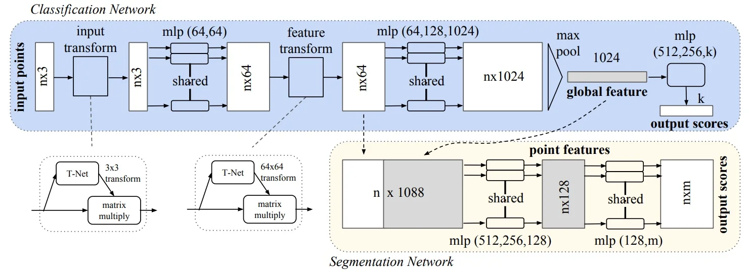
Pose Normalization via T-Net Modules To improve invariance to arbitrary spatial transformations, PointNet incorporates two optional Transformation Networks (T-Nets) that learn to align both the input point cloud and its intermediate feature representations to canonical frames.
- Input T-Net: This module predicts a spatial alignment for the raw coordinates \( \mathcal {P} \in \mathbb {R}^{P \times 3} \). It follows the PointNet architecture—shared MLPs, max-pooling, and fully connected layers—to regress a \( 3 \times 3 \) transformation matrix, which is then applied directly to the input points. This normalization step removes global rotation and translation ambiguity, ensuring that the downstream network processes consistently oriented data.
-
Feature T-Net: A second T-Net operates on the intermediate per-point feature vectors (e.g., after the first shared MLP), predicting a \( D \times D \) transformation matrix to align feature embeddings in the latent space. This matrix is applied before aggregation, improving the stability and semantic consistency of learned features across different object poses and variations.
- Regularization: To ensure that the predicted feature transformation is approximately orthogonal (i.e., preserves information), a regularization loss of the form \[ L_{\mathrm {reg}} = \left \| I - A A^\top \right \|_F^2 \] is added to the training objective, where \( A \in \mathbb {R}^{D \times D} \) is the predicted transformation matrix and \( \| \cdot \|_F \) denotes the Frobenius norm.
By learning to normalize both geometric and feature-level representations, these T-Net modules enhance the model’s robustness to pose variation and improve the reliability of downstream classification or segmentation predictions.
Hierarchical Reasoning via Iterative Refinement Beyond the basic structure, subsequent variants of PointNet can perform multi-stage feature fusion:
- After the first max-pooling yields \( h_{\mbox{global}} \in \mathbb {R}^D \), it is concatenated with each point feature to form \( \mathbb {R}^{P \times 2D} \).
- A shared MLP processes these enriched per-point vectors.
- A second max-pooling generates a refined global descriptor.
- This sequence—concat, MLP, pooling—can be repeated multiple times, allowing the network to capture hierarchical, higher-order shape attributes.
This iterative deep set reasoning retains permutation invariance while progressively enhancing the model’s expressive power.
Legacy and Evolution PointNet demonstrated that symmetry-aware, set-based architectures can rival or surpass volumetric CNNs in classification and segmentation—while using significantly less memory and supporting higher-resolution geometry. Its simple yet powerful design has led to a series of influential extensions that form the backbone of modern 3D deep learning pipelines.
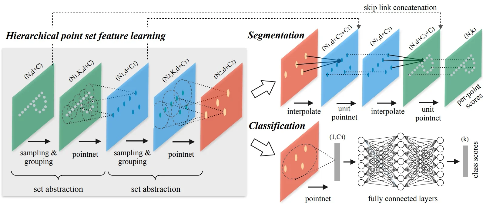
23.5.3 PointNet++: Hierarchical Feature Learning on Point Clouds
While PointNet [503] introduced a powerful set-based paradigm for point cloud processing, it suffers from a key limitation: the inability to explicitly model local geometric structures. Because PointNet aggregates all point features globally in a single pooling operation, it lacks sensitivity to fine-grained local patterns—much like trying to classify a shape without noticing its edges or corners.
PointNet++ [504] addresses this limitation by introducing a hierarchical architecture that recursively applies PointNet within spatially localized regions. This structure enables the model to learn point-wise features at progressively larger contextual scales, akin to how CNNs build up representations from local patches to full-image semantics.
The core architectural unit in PointNet++ is the Set Abstraction (SA) module, which consists of three main stages:
- 1.
- Sampling: From the full point set, a representative subset is selected as centroids of local regions. This is typically performed using Farthest Point Sampling (FPS), which ensures even spatial coverage of the point cloud by selecting points that are maximally distant from one another. This avoids clustering in high-density areas and helps capture the object’s full spatial extent.
- 2.
- Grouping: For each sampled centroid, a local neighborhood is defined. The standard method is a ball query, which includes all points within a fixed radius. This spatially bounded grouping ensures that the local features extracted are consistent and scale-aware. (Alternatively, \(k\)-nearest neighbors can be used, though ball queries preserve fixed spatial context).
- 3.
- PointNet Encoding: Within each local neighborhood, a mini-PointNet is applied—mapping the points into a local reference frame (relative to the centroid) and computing a feature vector via shared MLPs and symmetric max-pooling. This step captures local geometric properties such as curvature, edges, or flatness.
By stacking multiple SA modules, PointNet++ constructs a deep hierarchy of features—from local patches to global shape descriptors—allowing robust recognition of both coarse and detailed structure.
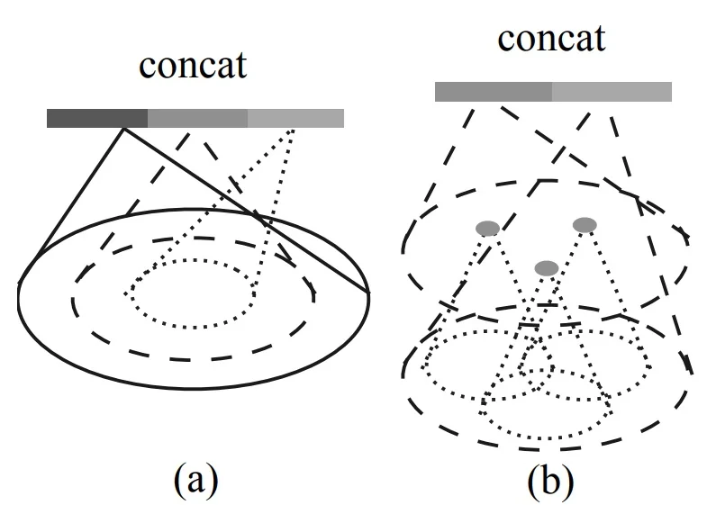
Density-Adaptive Grouping and Robustness A major challenge in real-world point clouds—such as those acquired via LiDAR or RGB-D sensors—is the presence of non-uniform sampling density. Nearby surfaces often result in dense clusters of points, while distant or occluded areas may be sparsely sampled. If a network uses a fixed-radius neighborhood (as in single-scale grouping), it may gather too few points in sparse regions (leading to unstable features), or be unnecessarily redundant in dense regions (wasting computation).
To address this, PointNet++ [504] introduces two density-adaptive grouping strategies that allow feature learning to adapt across varying sampling densities:
-
Multi-Scale Grouping (MSG): For each centroid in the set abstraction layer, MSG performs multiple ball queries of increasing radii (e.g., small, medium, large), forming concentric local neighborhoods of different scales. Each group is processed by a separate mini-PointNet, and the resulting feature vectors are concatenated into a unified multi-scale representation.
Intuition: In dense regions, small-radius neighborhoods suffice to capture fine detail; in sparse regions, larger-radius neighborhoods ensure geometric coverage. MSG makes the model robust to such density variations at the cost of increased computation due to multiple parallel branches.
-
Multi-Resolution Grouping (MRG): As a more efficient alternative, MRG leverages the hierarchical nature of PointNet++. At each level \(L_i\), the feature for a local region is computed by concatenating:
- a low-resolution feature from the previous level \(L_{i-1}\), summarizing a large, sparse context;
- a high-resolution feature from a mini-PointNet applied to the raw points in the local region at level \(L_i\).
This dual-path design allows the network to dynamically emphasize coarse or fine structure depending on local point density.
Intuition: When a region is well-sampled, detailed features from the current level dominate; when sparse, the network falls back on coarse summaries inherited from deeper layers.
Random Input Dropout: During training, PointNet++ further improves robustness by randomly dropping input points. This encourages the model to generalize across incomplete or sparsely sampled inputs—a common scenario in real-world 3D capture.
Feature Propagation for Dense Prediction For tasks like semantic segmentation—where per-point predictions are required—PointNet++ uses a feature propagation module to interpolate and upsample coarse features back to the original resolution. This is achieved via:
- Distance-weighted interpolation from nearby subsampled points.
- Skip connections from earlier levels in the hierarchy.
This ensures that each point benefits from both its raw input and the abstracted global features accumulated through the hierarchy.
Summary and Impact PointNet++ marks a major evolution in point cloud learning. By extending PointNet with hierarchical spatial reasoning, local neighborhood modeling, and density-aware design, it achieved state-of-the-art performance across classification, segmentation, and 3D object detection benchmarks at its time of publication. The hierarchical Set Abstraction modules provide a powerful and general-purpose building block for modern geometric deep learning pipelines.
Extensions and Improvements Numerous architectures have extended the PointNet++ paradigm to enhance expressiveness, efficiency, and scalability:
- PointNeXt [505] revisits PointNet++ with modern training techniques, simplified blocks, and residual connections for improved accuracy.
- DGCNN [706] introduces dynamic edge convolutions over local graphs, capturing fine-grained geometric relations across neighboring points.
- Point Transformers [807, 727] apply attention mechanisms to model long-range interactions in the point set, enabling context-aware reasoning.
These models now underpin many 3D perception systems, spanning applications in classification, segmentation, shape generation, and scene understanding.
Toward Structured Representations While point clouds offer an efficient and flexible surface representation, they lack explicit connectivity. This motivates the transition toward structured outputs such as triangle meshes and implicit surfaces, which support physically grounded operations like rendering, simulation, and editing.
23.6 Triangle Meshes for 3D Shape Modeling
Triangle meshes are among the most widely used representations for 3D shapes in computer graphics, simulation, and geometric learning. A triangle mesh explicitly defines the surface of a 3D object using a finite set of vertices and faces. Let \(\mathcal {V} = \{ \mathbf {v}_i \in \mathbb {R}^3 \mid i = 1, \ldots , V \}\) denote the set of 3D vertex coordinates, and let \(\mathcal {F} = \{ (i, j, k) \mid i, j, k \in [1, V] \}\) denote the set of triangular faces, each indexed by three vertices.
This representation defines a piecewise-linear manifold embedded in 3D, enabling efficient rendering and geometric reasoning. Each face defines a planar triangle bounded by edges, and the entire mesh approximates a continuous surface.
Advantages of Triangle Meshes Triangle meshes are the standard in real-time and offline 3D applications due to several key properties:
- Surface explicitness: Meshes represent the actual 2D surface geometry embedded in 3D, facilitating accurate surface-based computations such as rendering, shading, and physical simulation.
- Adaptive resolution: Large triangles can be used in smooth regions, while dense subdivisions can capture high-curvature or detailed regions, yielding compact yet expressive representations.
- Rich annotations: Meshes can carry per-vertex attributes such as surface normals, color, and texture coordinates, which are interpolated over the mesh faces for shading and alignment.
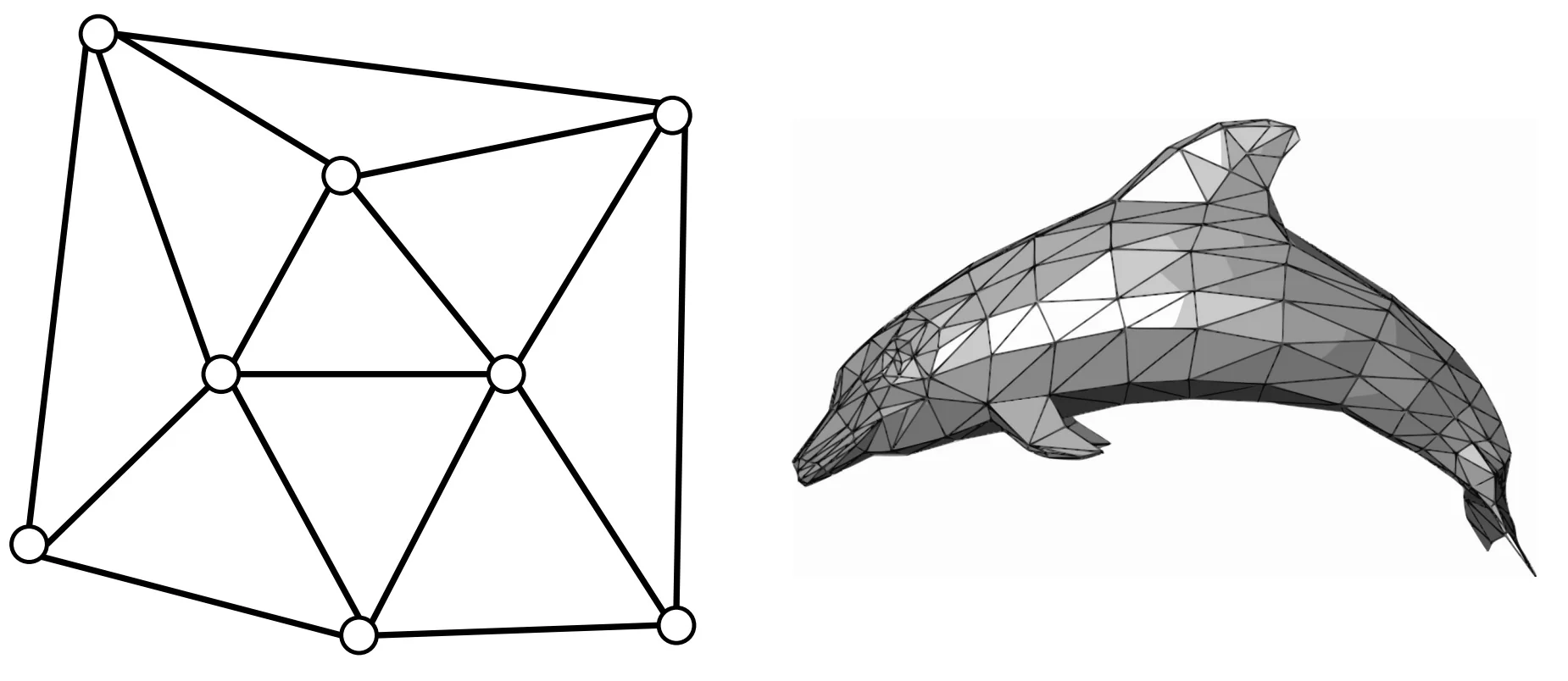
Despite their efficiency, predicting triangle meshes from raw data (e.g., RGB images or point clouds) presents significant challenges: the output structure is non-Euclidean, connectivity must be preserved, and operations such as upsampling or interpolation are nontrivial. The next subsection introduces a model that addresses these challenges through learned graph-based mesh deformation.
23.6.1 Pixel2Mesh: Predicting Triangle Meshes
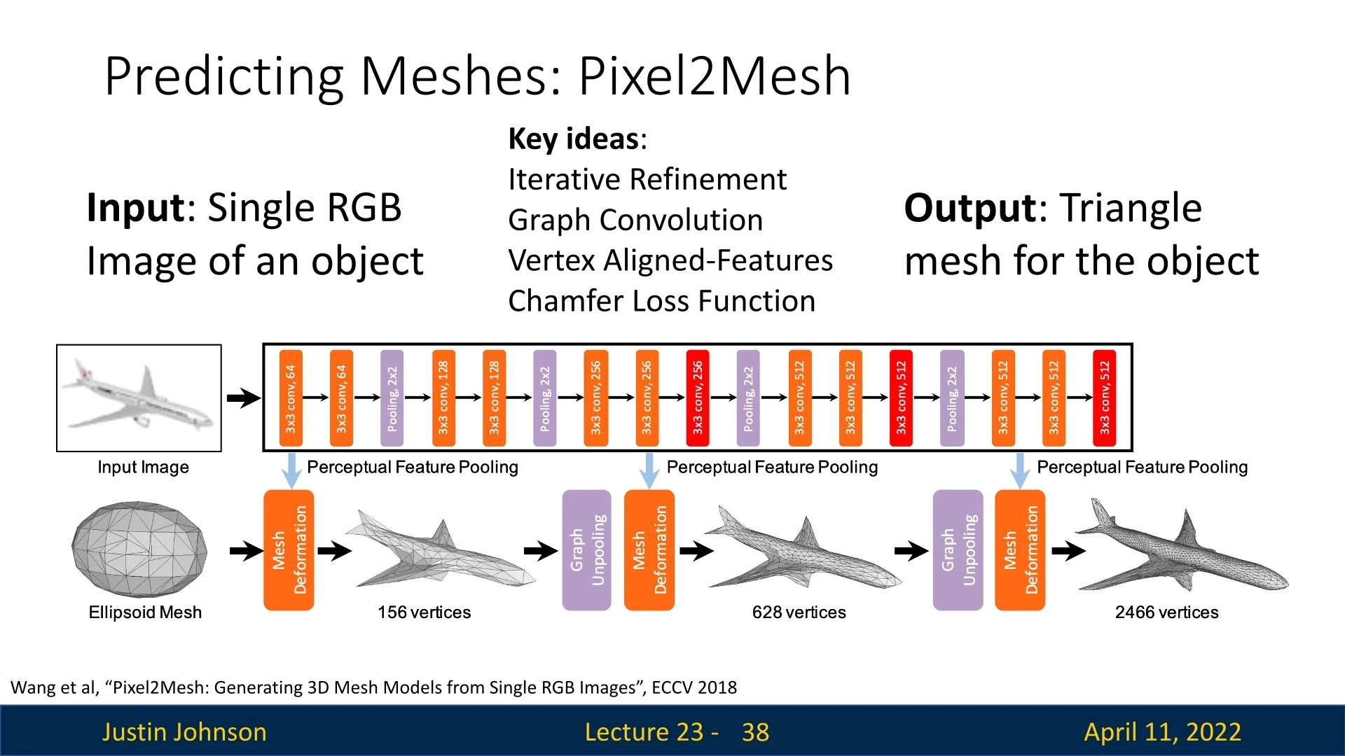
Pixel2Mesh [686] is a landmark method for generating 3D triangle meshes directly from a single RGB image. Unlike voxel-based approaches—which scale cubically in memory—or point cloud methods—which lack surface connectivity and require post-processing to extract usable geometry—Pixel2Mesh predicts structured mesh outputs: surfaces defined by vertices, edges, and faces. This makes it particularly suitable for applications that require explicit topology, such as simulation, CAD, or rendering.
Pre-Pixel2Mesh Landscape Prior to mesh-based methods, 3D learning architectures primarily explored two output formats:
- Voxel grids: Compatible with 3D convolutions and spatial reasoning, but constrained by high memory usage. Even modest resolutions (e.g., \(64^3\)) require hundreds of thousands of cells, limiting detail.
- Point clouds: More efficient and flexible, but inherently unstructured. Without connectivity, they cannot express surface geometry directly, making downstream tasks such as meshing or simulation error-prone.
Core Proposition Pixel2Mesh offers a structurally informed alternative by modeling 3D shape as a deformable mesh graph. Starting from a fixed-topology, genus-0 template (typically an ellipsoid), the network learns to iteratively deform vertex positions to match the object depicted in the image. This progressive refinement approach reframes the task: instead of generating structure from scratch, the model predicts residual displacements—small, local adjustments to an existing shape. This both simplifies learning and naturally preserves manifold topology, as the mesh’s connectivity remains unchanged across deformations.
Key Innovations Pixel2Mesh introduced a number of interlinked architectural ideas that made this formulation tractable:
- Coarse-to-Fine Refinement: The model deforms the mesh over multiple stages. After each deformation step, the mesh is upsampled—that is, each face is subdivided to increase resolution—enabling the network to model fine-grained surface detail while maintaining stability early on.
- Graph Convolution on Meshes: Deformations are computed using graph convolutional networks (GCNs), which aggregate information across neighboring vertices based on mesh connectivity. This allows localized, topology-aware reasoning.
- Vertex-Aligned Features: To connect 2D image content with the 3D mesh, the model projects each vertex onto the image plane and samples CNN features at the corresponding location. These features are passed to the GCN to guide deformation, grounding mesh updates in visual evidence.
-
Chamfer Distance for Mesh Supervision: Pixel2Mesh supervises mesh prediction by comparing the predicted vertex set \( \mathcal {V} \subset \mathbb {R}^3 \) to a ground-truth point cloud \( \mathcal {S}_{\mbox{gt}} \) using the symmetric Chamfer Distance: \[ \mathcal {L}_{\mbox{Chamfer}} = \sum _{x \in \mathcal {V}} \min _{y \in \mathcal {S}_{\mbox{gt}}} \|x - y\|_2^2 + \sum _{y \in \mathcal {S}_{\mbox{gt}}} \min _{x \in \mathcal {V}} \|x - y\|_2^2. \]
Although simple and differentiable, this loss only supervises vertex positions and ignores the interiors of mesh faces—potentially allowing distortions like sagging or warping between correctly placed vertices.
Later work, such as GEOMetrics [594], improves on this by comparing point clouds sampled from the entire predicted surface, offering finer surface-level supervision.
High-Level Pipeline Pixel2Mesh transforms a single RGB image into a 3D triangle mesh through a progressive mesh deformation pipeline that unifies convolutional image features and geometric mesh reasoning. The method begins with two inputs: a 2D image and a coarse, genus-0 mesh template (typically an ellipsoid centered in front of the camera). This template serves as the canonical starting point for all reconstructions and encodes strong priors on manifoldness and mesh topology.
The network refines this initial mesh in three stages, each consisting of deformation, unpooling, and feature update modules. The process is structured as follows:
- 1.
- Image Feature Extraction: A 2D convolutional backbone (e.g., VGG-16) processes the input RGB image to extract multi-scale feature maps from intermediate layers (e.g., conv3_3, conv4_3, conv5_3). These maps encode both low-level textures and high-level semantic patterns, offering a rich perceptual signal that guides the 3D reconstruction process.
- 2.
- Vertex-to-Image Feature Pooling: Each mesh vertex is projected onto the image plane using known camera intrinsics. At the projected 2D coordinates, features are bilinearly sampled from the image’s multi-level CNN maps and concatenated to the vertex’s current geometric descriptor. This projection-based pooling serves as the only available cue during inference, anchoring the 3D reconstruction to image evidence. It provides the graph network with localized appearance information, helping it decide where and how to displace each vertex and add detail.
- 3.
- Graph Convolution for Deformation: The mesh is represented as a graph, with vertices as nodes and edges defined by mesh connectivity. A Graph Convolutional Network (GCN) processes this structure, updating each vertex’s feature vector by aggregating information from its neighbors. The GCN is composed of multiple layers, expanding each vertex’s receptive field and enabling contextual reasoning across the surface. Crucially, the image-aligned features from the pooling step guide the GCN’s residual predictions—telling the network how to deform the shape in 3D to better match the visual evidence.
- 4.
- Graph Unpooling for Resolution Increase: To increase geometric detail, the mesh is upsampled after each deformation stage using edge-based unpooling. New vertices are inserted at the midpoints of edges, and connectivity is updated to preserve the mesh’s manifold structure. The positions and features of new vertices are initialized by averaging their endpoints, allowing the network to seamlessly enrich surface detail without altering global shape or topology.
- 5.
- Iterative Refinement: The refined mesh is passed through multiple deformation stages, each repeating the cycle of vertex-to-image feature pooling (Step 2), GCN-based displacement prediction (Step 3), and graph unpooling (Step 4). This iterative coarse-to-fine strategy begins with a low-resolution mesh that captures global structure—benefiting from short graph diameters and large effective receptive fields—and progressively increases resolution to recover fine surface details. As the mesh converges toward the target shape, vertex projections align more accurately with relevant regions in the image, enhancing the quality of sampled features and enabling increasingly precise geometric corrections at each stage.
This multi-stage architecture offers a powerful compromise between efficiency and fidelity. The low-resolution mesh allows efficient global shape reasoning in early layers, while unpooling introduces degrees of freedom necessary for high-resolution surface detail. By integrating 2D image cues at every stage and learning deformation through graph-based reasoning, Pixel2Mesh generates detailed, topologically consistent 3D meshes from a single image.
Graph-Based Feature Learning A core challenge in learning from 3D meshes is that they are non-Euclidean structures. Unlike images or voxels, which lie on regular grids with fixed-size neighborhoods and translation-invariant kernels, triangle meshes consist of irregularly connected vertices with no global coordinate frame. To apply learning methods to this setting, Pixel2Mesh treats the mesh as a graph \( \mathcal {G} = (\mathcal {V}, \mathcal {E}) \), where:
- Nodes (\( \mathcal {V} \)) are mesh vertices. Each vertex \( i \in \mathcal {V} \) is assigned a feature vector \( \mathbf {f}_i \in \mathbb {R}^d \), initialized using its 3D coordinates \( \mathbf {v}_i \in \mathbb {R}^3 \), and later enriched through graph-based message passing.
- Edges (\( \mathcal {E} \)) encode mesh connectivity. Two nodes \( i \) and \( j \) share an edge if their corresponding vertices are adjacent on a triangle face. This forms the local neighborhood \( \mathcal {N}(i) \) around each vertex.
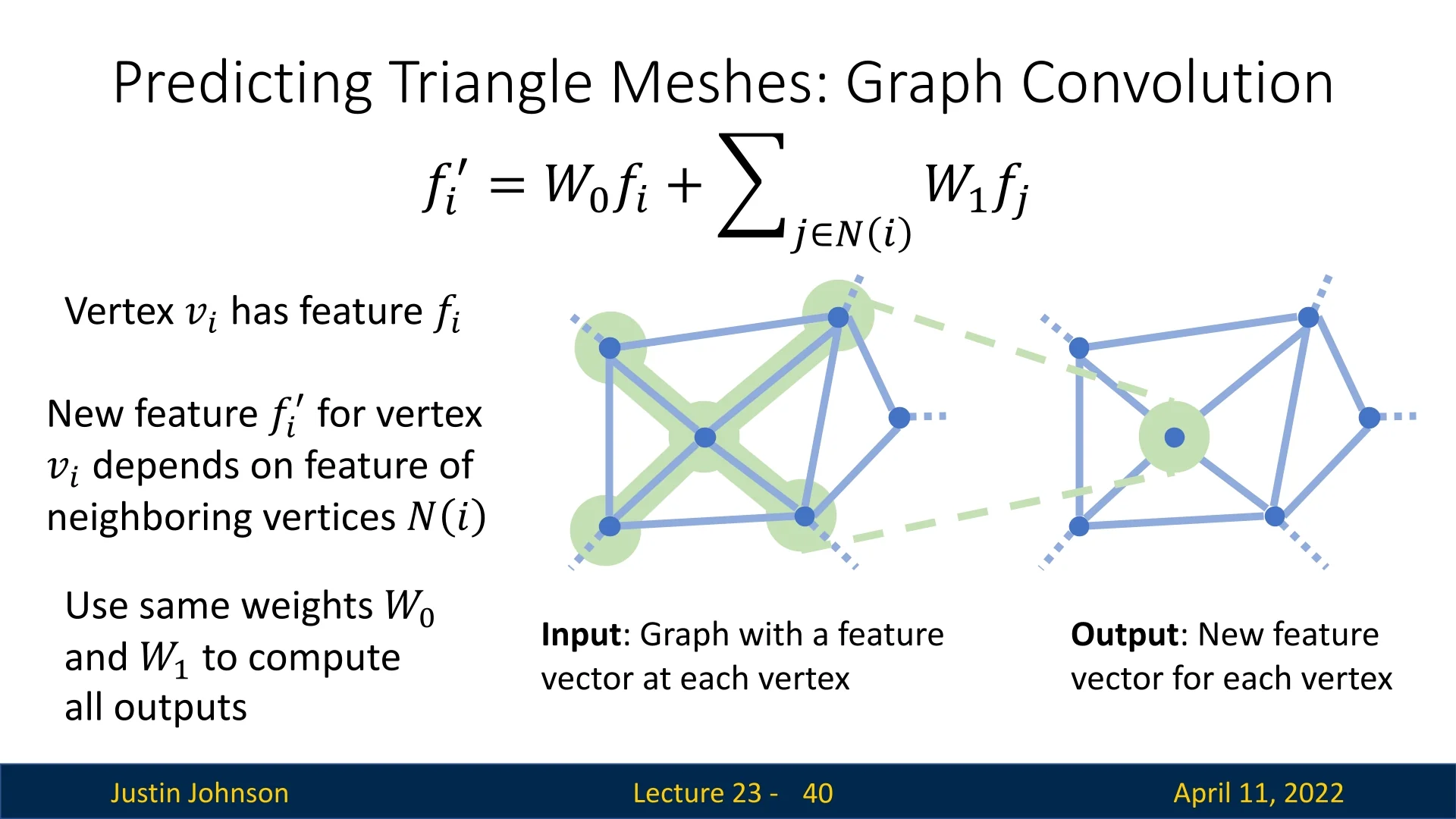
To extend the receptive field across the mesh and support complex shape reasoning, Pixel2Mesh stacks multiple such layers into a 14-layer Graph Convolutional ResNet (G-ResNet). The inclusion of residual (skip) connections helps stabilize optimization, facilitates deeper architectures, and allows low-level geometry to be preserved and reused throughout the network. As features propagate through the GCN, each vertex gains access to increasingly broader geometric context—essential for learning coherent deformations informed by both local surface cues and global object structure.
This graph-based feature hierarchy ultimately enables each vertex to predict a residual 3D displacement vector \( \Delta \mathbf {v}_i \), which updates its position without altering mesh connectivity. Subsequent parts detail how these features are fused with 2D image evidence and used to deform the mesh toward the target shape.
To increase the expressive capacity of the network, Pixel2Mesh stacks 14 such layers into a deep Graph Convolutional ResNet (G-ResNet). This depth enables each vertex to aggregate information from increasingly distant nodes, expanding its receptive field over the graph. Unlike grids, graphs can have highly irregular connectivity, and so reaching distant vertices may require many layers of message passing. Skip connections—added between GCN layers—help mitigate this by stabilizing gradient flow during training and facilitating feature reuse. In the context of mesh deformation, these residual paths are particularly useful: they allow the network to retain low-level spatial signals (e.g., coarse geometry or symmetric structures) while progressively layering on fine-grained, high-level shape refinements.
Predicting Vertex Positions via Graph Projection At the end of each mesh deformation block, the G-ResNet outputs a refined feature vector \( \mathbf {f}_i \in \mathbb {R}^d \) for each vertex \( i \). These features encode both geometric structure (through message passing over the mesh) and semantic cues (through vertex-aligned image features). To convert these features into updated vertex coordinates, Pixel2Mesh applies a simple yet crucial operation: a final linear layer referred to as the graph projection layer.
Formally, the new 3D position of each vertex is predicted as: \[ \mathbf {v}_i^{\mbox{new}} = W_{\mbox{proj}} \mathbf {f}_i, \] where \( W_{\mbox{proj}} \in \mathbb {R}^{d \times 3} \) is a learnable weight matrix shared across all vertices. This transformation maps the high-dimensional vertex features directly into absolute 3D space.
Importantly, this step does not compute or apply a residual displacement. The network predicts the final 3D position outright. Although this may seem counterintuitive—many deformation-based models favor residual updates for stability—the Pixel2Mesh architecture learns this coordinate regression implicitly, leveraging the structured feature learning of the G-ResNet. The underlying mesh structure and feature propagation already encode strong geometric priors, making direct position regression viable and effective.
Throughout this process, the mesh’s topology remains fixed: only vertex positions are updated, not their connectivity. This allows each deformation block to operate over a stable graph structure while progressively refining the mesh surface. After this coarse shape is aligned with the image, graph unpooling increases mesh resolution by inserting new vertices at edge midpoints. Subsequent deformation blocks then focus on finer-scale geometry, aided by a denser mesh and more localized 2D image alignment.
Edge-Based Graph Unpooling for Mesh Resolution Refinement After each stage of coarse deformation, Pixel2Mesh increases the mesh resolution to allow more fine-grained geometric refinement. This is achieved via a carefully designed graph unpooling operation that avoids the artifacts common in naive subdivision schemes. Instead of inserting new vertices at triangle centroids (which creates low-degree, poorly connected nodes), Pixel2Mesh uses an edge-based unpooling strategy inspired by classical mesh subdivision methods.
The unpooling procedure is as follows:
- A new vertex is inserted at the midpoint of each edge in the mesh.
- This new vertex is connected to the two endpoints of the edge.
- For every triangle in the original mesh, the three mid-edge vertices are connected to form a new inner triangle.
This process subdivides each original triangle into four smaller triangles and preserves regularity in vertex degree and local topology. To initialize the features of the new mid-edge vertices, the network simply averages the features of the parent vertices: \[ \mathbf {f}_{\mbox{new}} = \frac {1}{2}(\mathbf {f}_i + \mathbf {f}_j), \] where \( i \) and \( j \) are the endpoints of the edge. This yields smooth and stable feature transitions for subsequent GCN layers.
This coarse-to-fine unpooling scheme allows Pixel2Mesh to expand its receptive field and prediction granularity in tandem. The three-stage pipeline uses meshes with 156, 628, and finally 2466 vertices—an architecture that mirrors the increasing complexity of the shape being reconstructed. Early blocks handle the “big picture,” while later blocks focus on refining sharp contours, smooth curvatures, and small geometric details.
Image-to-Mesh Feature Alignment A key innovation in Pixel2Mesh is its ability to guide 3D mesh deformation using 2D visual cues extracted from the input image. This involves bridging two fundamentally different data domains: the regular, grid-aligned structure of 2D images and the irregular, graph-based structure of 3D meshes. Pixel2Mesh realizes this connection through a Perceptual Feature Pooling module, which aligns each mesh vertex with semantically relevant image features and dynamically refines that alignment at each deformation stage.
The process begins with a pretrained VGG-16 network (frozen during training), used to extract multi-scale image features from the input RGB image. Features are taken from three intermediate layers—conv3_3, conv4_3, and conv5_3—which together capture both fine textures and abstract semantics. These layers yield feature maps at decreasing spatial resolutions and increasing channel dimensionality.
For each vertex \( i \) in the current mesh, the following steps are performed:
- 1.
- Projection to the Image Plane: The 3D vertex position \( \mathbf {v}_i = (x_i, y_i, z_i) \in \mathbb {R}^3 \) is projected to 2D image coordinates using known perspective camera intrinsics: \[ (u_i, v_i) = \left ( \frac {f_x x_i}{z_i} + c_x,\; \frac {f_y y_i}{z_i} + c_y \right ). \] This maps the 3D point to the location on the image where it is expected to appear.
- 2.
- Bilinear Feature Sampling: At each projected coordinate \( (u_i, v_i) \), bilinear
interpolation is applied to the VGG feature maps to retrieve
image-aligned descriptors. This interpolation ensures that features
can be sampled at subpixel resolution and maintains differentiability
throughout the pipeline.
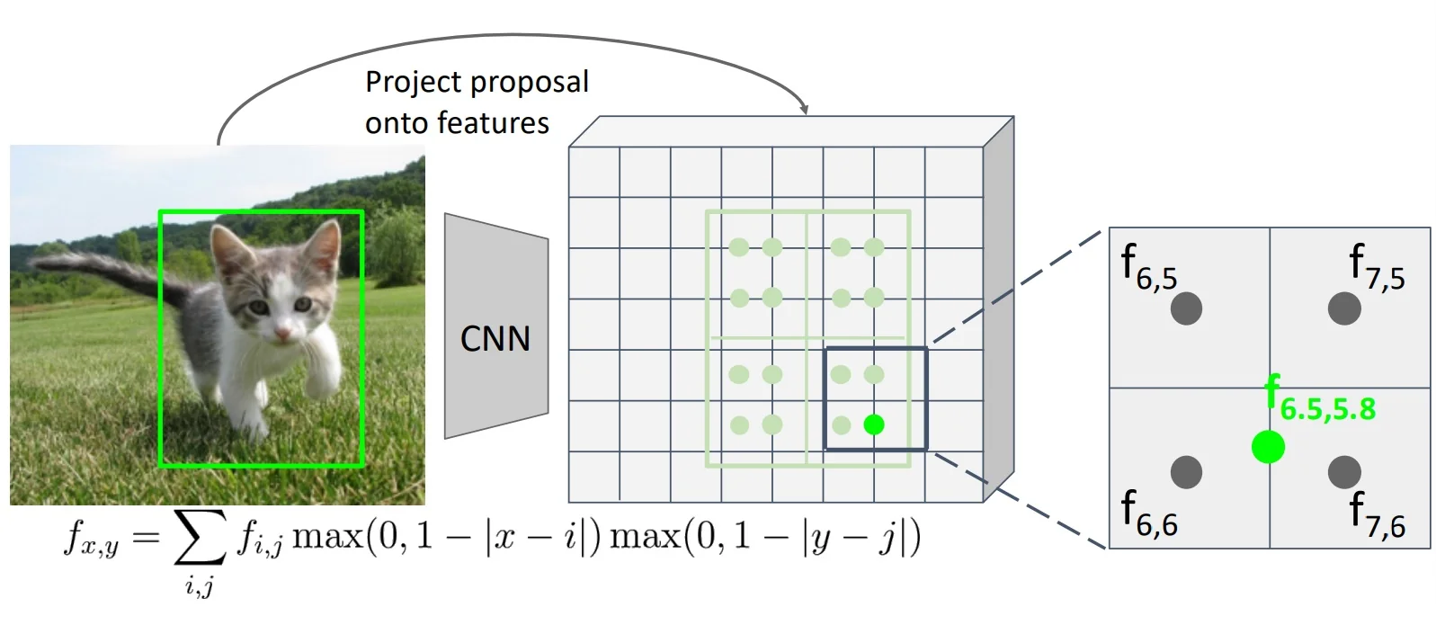
Figure 23.21: Bilinear interpolation retrieves CNN features at non-integer projected positions. This mechanism resembles RoIAlign and allows smooth vertex-to-image alignment. - 3.
- Multi-Scale Feature Fusion: The sampled feature vectors from conv3_3, conv4_3, and conv5_3 are concatenated to form a unified descriptor \( \mathbf {f}^{\mbox{img}}_i \in \mathbb {R}^{1280} \) (e.g., 256 + 512 + 512 channels). This vector encodes both local appearance and high-level semantics around the vertex projection.
- 4.
- Fusion with Graph Features: The perceptual feature \( \mathbf {f}^{\mbox{img}}_i \) is concatenated with the vertex’s geometric feature \( \mathbf {f}_i \in \mathbb {R}^d \), as computed by previous graph convolution layers. The resulting fused descriptor is then passed to the next G-ResNet deformation block to guide shape refinement.
Importantly, this perceptual pooling process is not static—it is repeated at the beginning of every mesh deformation block using the current mesh geometry. This creates a dynamic feedback loop:
- In the first stage, vertex projections from the initial ellipsoid are poorly aligned with the object, so pooled features are coarse and ambiguous.
- After the first deformation block updates vertex positions, the mesh becomes better aligned with the image.
- When pooling is reapplied in the next stage, projections land on more semantically meaningful image regions, yielding more informative features.
- This cycle continues, with improved mesh geometry enabling better feature alignment, which in turn enables more precise deformations.
This iterative loop—deform → reproject → repool—is central to Pixel2Mesh’s effectiveness. Rather than relying on static image features, the model continuously refines its 2D–3D correspondence, allowing later stages to make sharper, semantically aware deformations based on increasingly accurate visual cues. The tight coupling of image perception and geometric reasoning enables the network to generate high-fidelity 3D surfaces even from a single image input.
Loss Function for Mesh Prediction in Pixel2Mesh
To guide the deformation of a coarse mesh into a high-quality 3D reconstruction, Pixel2Mesh employs a composite loss function that balances geometric accuracy, surface regularity, and structural plausibility. The loss is applied not only to the final output but also at each intermediate stage in the coarse-to-fine refinement pipeline.
Primary Objective: Chamfer Distance (Vertex-to-Vertex) The central supervision signal is the symmetric Chamfer Distance between the predicted mesh vertices \( V_{\mbox{pred}} \) and a set of ground-truth vertices \( V_{\mbox{gt}} \), both sampled from respective meshes:
\[ \mathcal {L}_{\mbox{Chamfer}} = \sum _{v \in V_{\mbox{pred}}} \min _{u \in V_{\mbox{gt}}} \|v - u\|_2^2 + \sum _{u \in V_{\mbox{gt}}} \min _{v \in V_{\mbox{pred}}} \|u - v\|_2^2 \]
This term ensures that each predicted vertex lies close to some part of the ground-truth surface, and vice versa. While originally designed for unordered point sets, this metric is used here as a surrogate for surface similarity. It is efficient and differentiable, but has limitations—it evaluates only the positions of vertices and not the geometry of faces.
Laplacian Smoothness Loss To enforce local geometric coherence and prevent unrealistic surface artifacts, Pixel2Mesh introduces a Laplacian regularization term that encourages smooth vertex deformations. This loss penalizes deviations in the Laplacian coordinates of each vertex before and after deformation. The Laplacian coordinate of vertex \( i \) is defined as the offset between its position and the average of its immediate neighbors:
\[ \delta _i = \mathbf {v}_i - \frac {1}{|\mathcal {N}(i)|} \sum _{j \in \mathcal {N}(i)} \mathbf {v}_j \]
After a deformation block updates the mesh to new vertex positions \( \mathbf {v}_i' \), the updated Laplacian coordinate is denoted \( \delta _i' \). The Laplacian loss penalizes the change in these coordinates:
\[ \mathcal {L}_{\mbox{Lap}} = \sum _i \left \| \delta _i' - \delta _i \right \|_2^2 \]
This loss serves a dual purpose depending on the stage of mesh refinement. In early stages, when the mesh is still close to the initial ellipsoid, the Laplacian coordinates are small and uniform; the loss encourages smooth, globally consistent deformations, helping prevent tangled or self-intersecting geometry. In later stages, once the mesh has learned a plausible coarse shape, the Laplacian coordinates reflect learned local structure. Penalizing changes to these coordinates helps preserve previously learned surface details, ensuring that finer deformations do not overwrite or distort earlier predictions.
Intuitively, this loss encourages vertices to move together with their neighbors, discouraging isolated spikes, noisy fluctuations, or jagged artifacts—especially in high-curvature or thin regions. As such, it acts as a learned shape stabilizer throughout the deformation pipeline.
Edge Length Regularization As the mesh undergoes progressive refinement through unpooling, Pixel2Mesh introduces additional vertices and edges to increase spatial resolution. While this enables finer geometric detail, it also introduces new degrees of freedom that can destabilize the mesh—especially during early training or coarse-to-fine transitions. Without proper constraints, vertices may drift far from their neighbors, forming “flying vertices” connected by abnormally long edges. To suppress such artifacts, Pixel2Mesh applies an edge length regularization term, defined as:
\[ \mathcal {L}_{\mbox{edge}} = \sum _{(i,j) \in \mathcal {E}} \| \mathbf {v}_i - \mathbf {v}_j \|_2^2, \]
where \( \mathcal {E} \) is the set of all mesh edges at the current refinement stage. This loss penalizes the absolute squared length of each edge, thereby encouraging spatial coherence among neighboring vertices.
While this formulation is unnormalized in the original paper, its contribution to the overall loss is controlled via a fixed hyperparameter \( \lambda \), ensuring stability across deformation stages despite increasing edge count. Importantly, this term does not compare edge lengths to their prior values or enforce a canonical length. Instead, it acts as a dynamic local tether, discouraging over-extension without constraining the mesh to a rigid template.
This regularizer is especially critical immediately after graph unpooling. Newly added vertices—typically initialized at edge midpoints—are still trainable and unconstrained by prior geometry. The edge length loss ensures that their deformations remain consistent with the surrounding structure, preventing unstable stretching and promoting uniform vertex spacing.
Together with the Laplacian and normal consistency terms, this loss helps maintain the integrity of the mesh during deformation, guiding the network toward smooth, coherent, and physically plausible reconstructions.
Normal Consistency Loss To enhance visual quality and ensure correct surface orientation, a normal loss penalizes misalignment between predicted edges and ground-truth normals:
\[ \mathcal {L}_{\mbox{normal}} = \sum _i \sum _{j \in \mathcal {N}(i)} \left \langle v_i - v_j, \, n_q \right \rangle ^2 \]
Here, \( n_q \) is the normal at the closest point \( q \) on the ground-truth mesh to vertex \( v_i \). This loss encourages edges to lie tangent to the surface, improving shading behavior and geometric realism. It captures higher-order consistency beyond just vertex positions.
Total Loss The final loss combines all components with fixed scalar weights:
\[ \mathcal {L}_{\mbox{total}} = \mathcal {L}_{\mbox{Chamfer}} + \lambda _1 \mathcal {L}_{\mbox{normal}} + \lambda _2 \mathcal {L}_{\mbox{Lap}} + \lambda _3 \mathcal {L}_{\mbox{edge}} \]
Pixel2Mesh uses \(\lambda _1 = 1.6 \times 10^{-4}\), \(\lambda _2 = 0.3\), and \(\lambda _3 = 0.1\). These weights were selected empirically to ensure that geometric fidelity is prioritized while still promoting mesh regularity and perceptual realism.
Limitations and Future Directions While this loss formulation is effective, it has several shortcomings:
- Vertex-Only Supervision: The Chamfer loss evaluates only discrete vertex positions, not the full surface defined by mesh faces.
- Sagging Faces: Large triangles may sag or bulge between correctly placed corner vertices without incurring loss, as interior deviations are unobserved.
- Oversmoothing Risk: The combination of Laplacian and edge constraints may suppress sharp features or fine details if not balanced carefully.
- Triangulation Bias: Matching based on vertex positions can penalize geometrically similar surfaces with differing connectivity.
Later methods such as GEOMetrics address these issues by introducing surface-based sampling and differentiable point sampling from triangle interiors, allowing more accurate and complete loss computation over the full mesh surface.
Enrichment 23.6.1.1: Differentiable Surface Sampling in GEOMetrics
Surface-to-Surface Comparison with Differentiable Sampling A central innovation in GEOMetrics is its replacement of vertex-based supervision with full surface-level comparison. Pixel2Mesh constrains only mesh vertex positions using a Chamfer loss against a fixed ground-truth point cloud, ignoring the geometry of the mesh faces that connect them. As a result, large triangles can sag or bulge without penalty as long as their corner vertices remain close to the sampled ground truth—leading to visible artifacts.
To resolve this, GEOMetrics computes a symmetric distance between dense point clouds sampled from the entire surface of both meshes. The primary loss during early training is the Point-to-Point Chamfer Distance: \[ \mathcal {L}_{\mbox{PtP}} = \sum _{p \in S_{\mbox{pred}}} \min _{q \in S_{\mbox{gt}}} \|p - q\|_2^2 + \sum _{q \in S_{\mbox{gt}}} \min _{p \in S_{\mbox{pred}}} \|q - p\|_2^2 \] Here, \( S_{\mbox{pred}} \) and \( S_{\mbox{gt}} \) are point clouds sampled online from the predicted and ground-truth meshes, respectively. This loss encourages every sampled point on one surface to be close to some point on the other, and vice versa—ensuring both coverage and correspondence. The symmetric form (sum of minimum distances in both directions) avoids degenerate solutions like mode collapse, where one shape covers the other but not vice versa.
Because sampling is performed over triangle interiors rather than vertex sets, \( \mathcal {L}_{\mbox{PtP}} \) is invariant to vertex count, mesh tessellation, or triangulation pattern—making it a true surface-level supervision signal.
Point-to-Surface Loss and Fine-Tuning While \( \mathcal {L}_{\mbox{PtP}} \) is efficient and effective early in training, it remains an approximation: it compares discrete samples rather than true surfaces. During fine-tuning—the later stage of training when coarse structure has converged—GEOMetrics switches to the more precise Point-to-Surface loss: \[ \mathcal {L}_{\mbox{PtS}} = \sum _{p \in S_{\mbox{pred}}} \min _{f \in \mathcal {F}_{\mbox{gt}}} \mbox{Dist}(p, f)^2 + \sum _{q \in S_{\mbox{gt}}} \min _{f' \in \mathcal {F}_{\mbox{pred}}} \mbox{Dist}(q, f')^2 \] This loss computes the squared distance from each sampled point to the nearest triangle face on the opposing mesh, rather than to another sampled point.
This leads to a more geometrically faithful signal, especially in regions where faces are large or sparsely sampled—e.g., flat areas or sharp edges. By comparing to the continuous mesh surface (via face planes), \( \mathcal {L}_{\mbox{PtS}} \) avoids underestimating distances due to poor sampling density, making it better suited for high-precision surface alignment during final optimization.
Differentiable Surface Sampling via Reparameterization To ensure end-to-end differentiability, GEOMetrics samples surface points from the predicted mesh using a two-stage stochastic procedure:
- Area-weighted face selection: Each triangle is selected with probability proportional to its area, ensuring uniform sampling over the surface.
- Barycentric sampling: For a triangle with vertices \( v_1, v_2, v_3 \), a sample point \( r \) is drawn using: \[ r = (1 - \sqrt {u}) v_1 + \sqrt {u}(1 - w) v_2 + \sqrt {u} w v_3, \quad u, w \sim \mathcal {U}(0, 1) \]
This formula produces points uniformly distributed over triangle interiors. Crucially, \( r \) is a smooth function of the triangle vertices and the sampled random variables \( u, w \). Through the reparameterization trick—where \( u, w \) are held fixed during backpropagation—gradients from the loss propagate cleanly to the vertex positions. This makes it possible for the model to learn mesh geometry from supervision applied directly to its surface.
In practice, thousands of points (typically 3k–10k) are sampled per mesh per iteration, enabling fine-grained geometric feedback across the full predicted surface. This helps eliminate artifacts such as sagging triangles or curvature mismatches that would go unnoticed under vertex-only supervision.
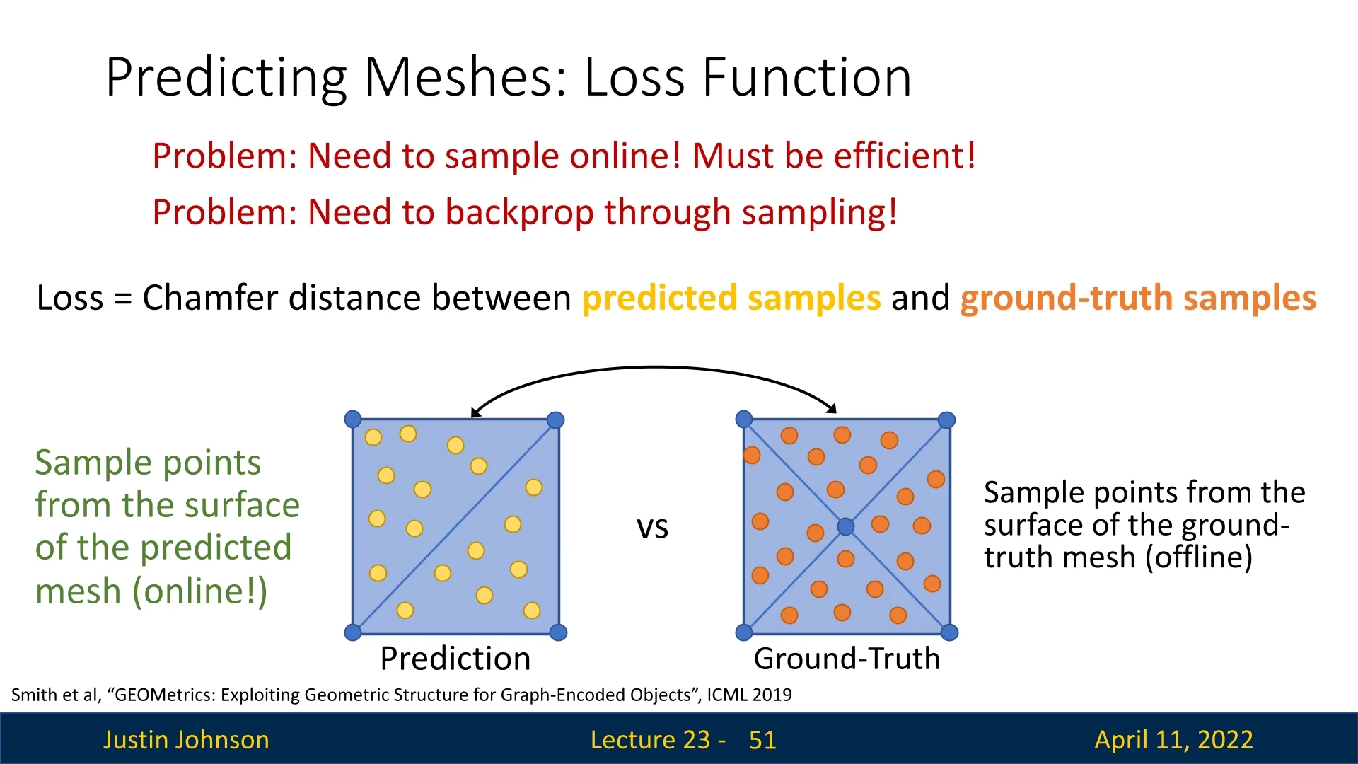
Complete Loss Formulation in GEOMetrics Beyond surface alignment, GEOMetrics incorporates two additional regularizers for mesh quality:
- Edge Length Regularization \( \mathcal {L}_{\mbox{edge}} \): discourages stretched edges and flying vertices.
- Laplacian Regularization \( \mathcal {L}_{\mbox{lap}} \): promotes local smoothness by minimizing differences between a vertex and the average of its neighbors.
The complete training objective is: \[ \mathcal {L}_{\mbox{total}} = w_1 \mathcal {L}_{\mbox{PtS}} + w_2 \mathcal {L}_{\mbox{edge}} + w_3 \mathcal {L}_{\mbox{lap}} + w_4 \mathcal {L}_{\mbox{latent}} \] where \( \mathcal {L}_{\mbox{latent}} \) is a perceptual loss that encourages global structural consistency using an auxiliary mesh-to-voxel autoencoder. Weights \( w_i \) are fixed scalars tuned for empirical balance.
Adaptive Mesh Refinement via Face Splitting Perhaps even more impactful than its loss function is GEOMetrics’ ability to adaptively modify mesh topology. Unlike Pixel2Mesh, which deforms a mesh with fixed vertex count and connectivity, GEOMetrics dynamically adds new vertices and faces during training. It identifies high-curvature or high-error regions and splits faces accordingly—concentrating resolution where it is needed most. This allows GEOMetrics to capture sharp details and fine contours without overloading flat regions with unnecessary vertices, leading to more efficient and expressive meshes.
This synergy between:
- accurate surface-level supervision.
- adaptive geometric capacity.
is what enables GEOMetrics to surpass previous models like Pixel2Mesh++ in reconstruction fidelity.
Advantages Over Vertex-Based Supervision Unlike Pixel2Mesh’s vertex-to-point Chamfer loss, GEOMetrics’ point-to-point surface loss:
- Supervises the entire surface, including triangle interiors.
- Handles varying mesh resolutions, as supervision is decoupled from vertex count.
- Respects valid geometric variation, allowing alternative triangulations of the same surface to be treated equally.
- Provides dense feedback, improving training stability and reconstruction fidelity.
Combined with adaptive face splitting, this loss enables GEOMetrics to produce smoother, more accurate, and topologically robust 3D shapes—closely matching the true surface geometry and not just sparse surface samples.
Limitations of Pixel2Mesh and the Motivation for Successor Models
While Pixel2Mesh introduced a landmark approach to deforming 3D meshes from a single RGB image using graph-based convolutions, several fundamental limitations restrict its generality and reconstruction quality. These include limited supervision, fixed-topology constraints, and reliance on single-view input. Each of these weaknesses directly motivated the development of successor models such as Pixel2Mesh++ [712] and Mesh R-CNN [183].
Single-View Ambiguity and 2.5D Reconstruction Pixel2Mesh is designed for single-view reconstruction. As a result, it struggles to infer geometry for regions not visible in the input image—such as the back of a chair or the underside of a car—because no direct pixel-level evidence is available. The model must hallucinate plausible completions from learned priors, often leading to reconstructions that appear reasonable from the input view but become implausible from novel viewpoints. This limitation manifests as a 2.5D facade, where only the visible surfaces are accurate.
Pixel2Mesh++ [712] addresses this challenge by introducing a multi-view deformation network, which jointly optimizes mesh refinements over multiple input images with known camera poses. This enforces cross-view consistency, improves alignment across viewpoints, and reduces ambiguity from occluded regions—ultimately producing shapes that are globally correct, not just front-facing.
Topological Rigidity and the Genus-0 Constraint Because Pixel2Mesh deforms a fixed ellipsoid mesh, it inherits a genus-0 topology by design. The graph unpooling operations add vertices and increase resolution, but never alter the global connectivity. As such, the model cannot represent structures with holes, handles, or disconnected components (e.g., mugs, chairs, or lamps).
This motivated the development of Mesh R-CNN [183], which replaces template deformation with a two-stage voxel-to-mesh pipeline. A coarse voxel occupancy grid is first predicted and then converted into a mesh using a differentiable surface extraction method. This allows the resulting mesh to assume arbitrary topology—including high-genus structures—removing the restrictive genus-0 bottleneck entirely.
Surface-Level Supervision and Over-Smoothing Limitations Pixel2Mesh originally supervised mesh deformation by applying the symmetric Chamfer Distance between predicted vertex positions and a pre-sampled ground-truth point cloud. While effective for guiding coarse shape, this vertex-only supervision ignores the faces connecting the vertices. As a result, the model can produce meshes where the corners of triangles are well-aligned, yet the interiors may sag or bulge—creating visibly inaccurate geometry that incurs no loss penalty.
This deficiency is exacerbated by the use of strong regularizers—such as Laplacian and edge length losses—which encourage smooth deformations. Combined with the inherently diffusive nature of graph convolutions, these constraints often lead to over-smoothed reconstructions that lack sharp creases, high-frequency detail, or geometric precision in sparsely sampled regions.
Pixel2Mesh++ [712] directly addresses this issue by incorporating a resampled surface-level Chamfer loss. Instead of comparing vertex coordinates, it samples dense point clouds from the predicted mesh surface using area-weighted barycentric sampling and computes the Chamfer loss against the ground-truth surface. This resampling improves gradient coverage over the full mesh and provides more reliable supervision in regions with irregular tessellation or thin structures.
GEOMetrics [594] builds further on this idea by introducing fully differentiable sampling operations and designing losses that explicitly evaluate surface-to-surface geometry. Its Point-to-Point (PtP) loss compares dense sampled point clouds, while the more refined Point-to-Surface (PtS) loss measures exact distances from predicted points to ground-truth triangle faces—yielding higher fidelity and stronger surface alignment. These losses not only address sagging artifacts, but also resolve ambiguities due to vertex layout or triangulation mismatches.
While both Pixel2Mesh++ and GEOMetrics move beyond vertex-based loss functions, the key distinction lies in formulation. Pixel2Mesh++ retains the Chamfer framework but improves its application via surface sampling; GEOMetrics reformulates the loss to reflect the mesh’s implicit surface, enabling direct point-to-face supervision.
Domain Shift and Real-World Generalization Trained primarily on synthetic datasets like ShapeNet, Pixel2Mesh suffers from a domain gap when tested on real-world imagery. Lighting variation, clutter, occlusion, and camera calibration errors can all destabilize the vertex-to-image feature alignment step. This leads to inconsistent updates and poor reconstruction quality in natural scenes.
Mesh R-CNN [183] takes a different route: by grounding its pipeline in instance detection via Mask R-CNN, it gains robustness to diverse, real-world input. Mesh generation is conditioned on high-confidence 2D detections, improving generalization to cluttered, multi-object scenes.
Summary and Takeaways Pixel2Mesh introduced a foundational framework for 3D mesh reconstruction from single RGB images, combining graph-based deformation, vertex–image alignment, and progressive refinement. However, key limitations—including its reliance on single-view input, fixed genus-0 template topology, and vertex-only supervision—highlighted the need for more flexible and accurate approaches.
The first evolution in this direction was Pixel2Mesh++ [712], which enriched the original framework without discarding its template-based foundations. By incorporating multi-view image input and surface-aware losses via differentiable mesh sampling, it improved geometric fidelity and alleviated ambiguity from occlusion and limited field-of-view—yet still operated under a fixed-topology deformation regime.
More structurally transformative approaches soon followed:
- GEOMetrics [594] enhanced surface-level supervision through dense differentiable sampling and adaptive face splitting. This resolved vertex sparsity and sagging-face artifacts while enabling targeted geometric refinement—but remained limited to low-genus templates.
- Mesh R-CNN [183] broke free from the fixed-topology constraint altogether. By predicting voxel-based occupancy maps followed by mesh extraction and refinement, it enabled the generation of arbitrary topology—including holes, handles, and disconnected parts—marking a major departure from template-based reconstruction.
Together, these successor models reflect a progression: from enriching Pixel2Mesh with multi-view cues and improved losses, to redefining the reconstruction pipeline entirely. As we now transition to Mesh R-CNN, we will see how voxel-driven, detection-aware pipelines offer a powerful alternative for general-purpose, topology-flexible 3D mesh reconstruction.
23.6.2 Mesh R-CNN: Topology-Aware Mesh Reconstruction from Real-World Images
Motivation and Key Ideas Traditional mesh reconstruction pipelines, such as Pixel2Mesh (Section 23.6.1), deform a fixed-topology template mesh (typically genus-0), which fundamentally limits their capacity to represent real-world objects with topological complexity—such as holes, multiple parts, or disconnected components.
Mesh R-CNN [183] introduces a hybrid reconstruction paradigm that overcomes this limitation by integrating two complementary representations:
- A voxel-based prediction branch first estimates a coarse 3D shape from the input image. Since voxel grids are regular and topology-agnostic, this stage can represent arbitrary structures, including objects with holes or non-manifold parts.
- A mesh refinement branch then converts the voxel output into a triangular mesh and applies graph-based neural operations to improve surface fidelity and geometric detail.
While voxel grids offer topological flexibility, they suffer from low resolution and quantization artifacts due to memory constraints. Mesh R-CNN resolves this by converting the voxel output into a surface mesh using the cubify operation, and then refining the mesh using a graph convolutional network (GCN). This two-stage process combines the strengths of volumetric and surface-based approaches: arbitrary topology from voxels, and high-resolution detail from meshes.
The entire system is trained end-to-end using paired RGB images and watertight 3D meshes, enabling amodal 3D shape prediction even in the presence of occlusion.
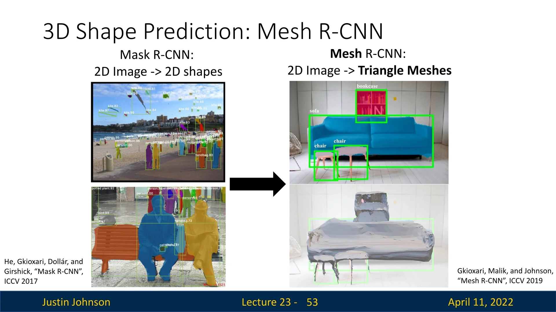
Mask R-CNN as Backbone for 2D Instance Segmentation Mesh R-CNN builds on the Mask R-CNN architecture introduced in Section §13, which performs 2D object detection and instance segmentation by augmenting Faster R-CNN with a pixel-level segmentation head. Given an input image, Mask R-CNN produces:
- Bounding box proposals for object instances.
- RoI-aligned feature maps for each proposal.
- Binary segmentation masks and class labels for each instance.
Mesh R-CNN inherits these components and reuses RoI-aligned features to bootstrap 3D shape prediction in the following stages.
The Mesh Prediction Head: A Hybrid Voxel-to-Mesh Strategy With Mask R-CNN as its 2D perception backbone (Section §14), Mesh R-CNN augments this architecture with a dedicated 3D shape prediction branch, called the mesh head. This component reconstructs a full 3D mesh for each detected object instance and is designed to balance topological flexibility with geometric precision.
The key architectural insight is to decompose the reconstruction task into two complementary and end-to-end trainable stages:
- 1.
- Voxel Prediction: For each object detected by Mask R-CNN, a coarse 3D occupancy grid is predicted from RoI-aligned image features. This voxel grid serves as a topology-agnostic representation that can naturally encode complex structures—including holes, thin parts, and disconnected components—without being constrained by mesh connectivity or genus. Because voxel occupancy is defined per grid cell, this stage supports per-instance reconstructions with arbitrary and varying topology.
- 2.
- Mesh Refinement: The predicted voxel grid is converted into a watertight triangle mesh using a dedicated cubify operation, which replaces each occupied voxel with a triangulated cuboid, merges shared vertices and edges, and removes interior faces. This produces an initial mesh whose topology directly mirrors the voxelized shape. To improve geometric fidelity, the mesh is then refined by a sequence of graph convolutional layers that deform vertex positions while preserving the established connectivity.
This voxel-to-mesh pipeline addresses a major limitation of prior methods like Pixel2Mesh, which were constrained to deforming a single genus-0 template mesh and thus unable to represent objects with complex topologies. By deferring mesh construction until after a coarse shape has been predicted, Mesh R-CNN avoids prematurely committing to a fixed topology and instead enables the reconstruction of multiple, topologically diverse meshes—one per detected instance—even from a single input image.
Crucially, the voxel and mesh branches are trained jointly within a fully differentiable framework. The voxel grid is supervised via a binary occupancy loss, while the mesh is optimized using surface-level objectives such as Chamfer distance, normal consistency, and edge regularization (all seen previously with Pixel2Mesh). This tight integration enables the system to learn both what to reconstruct (via voxels) and how to reconstruct it accurately (via mesh refinement), resulting in high-quality 3D predictions that generalize across diverse object categories and scene configurations.
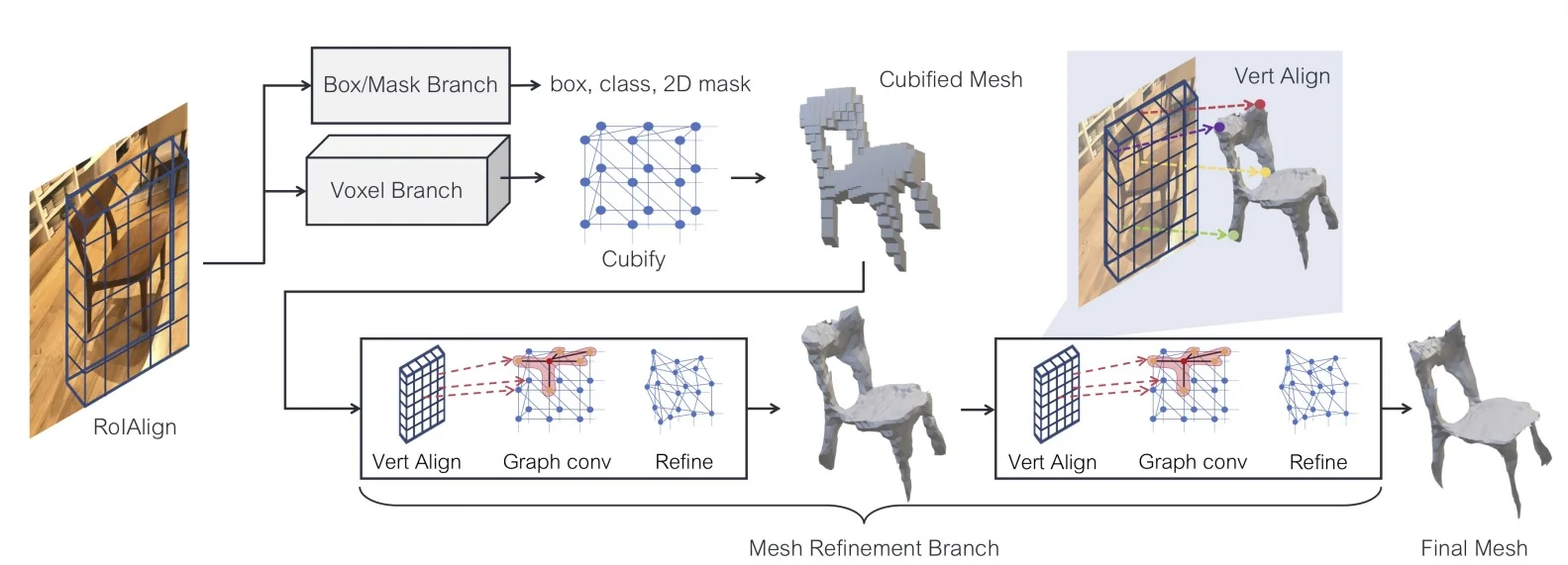
The Voxel Branch for Topological Flexibility
The first stage of the mesh head in Mesh R-CNN is the voxel prediction branch, which estimates a coarse 3D shape for each detected object as a voxel occupancy grid. Voxel representations are topology-agnostic by construction: they impose no constraints on surface connectivity and can naturally represent complex geometric structures—including holes, disconnected components, and non-manifold parts—without requiring a mesh template. This stands in contrast to methods like Pixel2Mesh (Section 23.6.1), which deform a fixed-topology genus-0 sphere and thus cannot model diverse shape topologies.
In Mesh R-CNN, the voxel branch uses RoI-aligned features from the Mask R-CNN backbone to predict occupancy probabilities over a grid of shape \( G \times G \times G \), where \( G = 24 \) or \( 48 \) depending on the dataset. Specifically, \( G = 48 \) is used for synthetic datasets like ShapeNet, while \( G = 24 \) is used for real-image datasets like Pix3D to manage memory constraints. Each voxel \( (i,j,k) \) receives a scalar logit, which is transformed via a sigmoid activation into an occupancy probability \( p^{\mbox{pred}}_{ijk} \in [0,1] \). This probabilistic grid forms a coarse but flexible volumetric scaffold that directly determines the topology of the output mesh in the next stage.
Perspective-Aware Voxel Grid via Camera Frustum Alignment To ensure metric grounding and spatial consistency, Mesh R-CNN defines its voxel grid within a camera-aligned 3D frustum. This volume is constructed using the predicted 2D bounding box and known camera intrinsics \( K \), anchoring the 3D grid in true physical coordinates rather than in an arbitrary canonical frame. The process consists of two phases: constructing the 3D voxel volume, and populating it with 2D-aligned features.
Phase 1: Constructing the Frustum-Aligned Voxel Grid
- Step 1:
- Defining the Frustum Volume. Given a Region of Interest (RoI)
bounding box \[ \mathcal {B} = (u_{\min },\; v_{\min },\; u_{\max },\; v_{\max }), \] and a known camera intrinsics matrix \( K \), Mesh R-CNN
constructs a perspective frustum in 3D by back-projecting the four
image-plane corners of \( \mathcal {B} \) using \( K^{-1} \). Each back-projected ray originates at
the camera center and passes through a bounding box corner, defining
the edges of the viewing frustum.
To bound the depth extent of the object, these rays are truncated between near and far depth planes, \( z_{\mbox{near}} \) and \( z_{\mbox{far}} \), which define the front and back clipping planes of the frustum. These values are not fixed in the paper but are dataset-dependent; for example, values like \( 0.5 \)m to \( 2.5 \)m may be used for indoor objects, while normalized scales are often applied for datasets like ShapeNet. The key point is that the frustum adapts to the RoI and camera parameters, ensuring that the predicted voxel grid aligns with the object’s visible volume in camera coordinates.
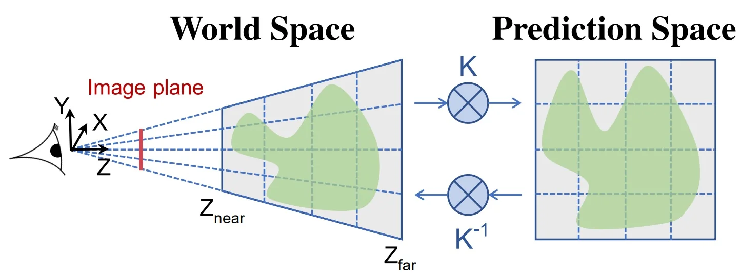
Figure 23.26: Frustum-aligned prediction space in Mesh R-CNN. Rather than predicting occupancy in a uniform world-aligned cube, Mesh R-CNN defines voxel predictions in a space aligned with the image plane. This is achieved by applying the camera intrinsics matrix \( K \) during voxel warping; applying \( K^{-1} \) transforms the voxel coordinates back into 3D world space. The result is a truncated frustum bounded by near and far depth planes (\( z_{\mbox{near}}, z_{\mbox{far}} \)), centered on the detected object. This frustum-aware grid mirrors the actual viewing volume of the camera, ensuring that voxel resolution is higher for nearby regions and coarser at greater depths—naturally encoding perspective and spatial priors. For background on camera intrinsics and perspective projection, see [588]. Figure adapted from Gkioxari et al. [17]. - Step 2:
- Canonical Grid Initialization. A logical voxel grid \( \mathcal {G} \in [-1,1]^3 \) is instantiated with
shape \( G \times G \times G \). This canonical cube serves as a resolution-independent coordinate
frame for voxel predictions. Each voxel index \( (i, j, k) \) is mapped to a normalized
position \( (x, y, z) \in [-1,1]^3 \), where:
- \( x = -1 \) denotes the leftmost extent and \( x = 1 \) the rightmost.
- \( y = -1 \) denotes the bottom and \( y = 1 \) the top.
- \( z = -1 \) corresponds to the front of the volume (near plane), and \( z = 1 \) to the back (far plane).
- Step 3:
- Perspective-Aware Warping. To map \( \mathcal {G} \) into the physical frustum, each
normalized coordinate \( (x, y, z) \) is transformed into a 3D point \( (X, Y, Z) \) using a homography
induced by the camera intrinsics and frustum geometry. This transformation
ensures:
- Voxels near the camera are tightly packed and represent small metric volumes.
- Voxels deeper in the frustum span larger volumes, mimicking perspective scaling.
This warping is applied before voxel prediction begins, allowing the 3D CNN to operate over a regular grid while producing perspective-consistent outputs.
Phase 2: Lifting 2D Features into 3D
Intuition. Rather than explicitly constructing a 3D feature volume, Mesh R-CNN leverages a fully-convolutional 2D network to infer 3D shape by predicting vertical voxel columns directly from RoI-aligned image features.
- Step 4:
- RoI Feature Extraction. The Mask R-CNN backbone provides RoI-aligned feature maps \( F \in \mathbb {R}^{C \times G \times G} \) for each object proposal, where \( G \) denotes the spatial resolution of the voxel grid along the horizontal and vertical image axes.
- Step 5:
- 2D Fully-Convolutional Prediction. A small 2D fully-convolutional network—analogous in structure to the Mask R-CNN mask head—is applied to \( F \) to produce an output tensor of shape \( G \times G \times G \). Here, each pixel location in the \( G \times G \) grid corresponds to a column of \( G \) occupancy logits along the depth axis of the voxel grid.
- Step 6:
- Voxel Probability Estimation. A sigmoid activation is applied to the output logits to obtain voxel-wise probabilities: \[ p_{ijk}^{\mbox{pred}} = \sigma (\ell _{ijk}) \quad \mbox{for all } (i,j,k) \in [0,G)^3, \] where \( \ell _{ijk} \) is the logit corresponding to voxel \( (i,j,k) \). The result is a perspective-aware, topology-flexible volumetric prediction aligned with the camera frustum.
Phase 3: Voxel Supervision and Mesh Conversion
Intuition. Starting from a voxel-aligned feature volume, we now convert the predicted occupancy grid into a coarse surface mesh. The cubify step transforms this discrete structure into a watertight mesh suitable for graph-based refinement.
- Step 7:
- Voxel-Wise Binary Cross-Entropy. The voxel prediction head
outputs a probability grid \( p^{\mbox{pred}} \in [0,1]^{G \times G \times G} \) representing the likelihood of occupancy at
each voxel location.
This is trained against a binary ground-truth volume \( p^{\mbox{gt}} \in \{0,1\}^{G \times G \times G} \) using voxel-wise binary cross-entropy: \[ \mathcal {L}_{\mbox{voxel}} = \frac {1}{G^3} \sum _{i,j,k} \mathrm {BCE}(p^{\mbox{pred}}_{ijk},\; p^{\mbox{gt}}_{ijk}). \] This encourages the network to produce a volumetric shape estimate that captures object structure and supports topological variation.
- Step 8:
- Thresholding the Occupancy Grid. At inference time, the predicted voxel probabilities are binarized using a fixed threshold \( \tau = 0.2 \), as used in the original Mesh R-CNN experiments on ShapeNet and Pix3D: \[ V_{ijk} = \mathbb {1}[p^{\mbox{pred}}_{ijk} > \tau ]. \] This produces a binary voxel occupancy grid \( V \in \{0,1\}^{G \times G \times G} \) that defines the object’s coarse 3D shape. Note: The threshold \( \tau \) can be adjusted per dataset to balance recall and precision, though \( 0.2 \) was found to work well empirically in the original evaluations [183].
- Step 9:
- Cubify: Voxel Grid to Watertight Mesh. The cubify operator [183]
transforms the binary voxel volume \( V \) into a triangle mesh \( \mathcal {M} = (\mathcal {V}, \mathcal {F}) \) using the following
procedure:
- Step 9:a.
- Cube Placement. For each occupied voxel \( V_{ijk} = 1 \), a unit cube is placed at grid location \( (i, j, k) \), consisting of 8 vertices and 12 triangle faces.
- Step 9:b.
- Face Culling. If a neighboring voxel in any of the six axial directions is also occupied, the shared face between cubes is removed. This avoids redundant geometry and ensures watertightness.
- Step 9:c.
- Vertex Merging. Once all cube faces are placed and pruned, duplicate vertices and edges are merged, yielding a coherent mesh with consistent connectivity and arbitrary topology.
Vectorized Cubify for Efficient Execution. A naive implementation of cubify would loop over all \( G^3 \) voxel cells, checking and processing each one. To make this practical for end-to-end training, Mesh R-CNN implements a fully vectorized version:
- The binary occupancy grid is convolved with small 3D kernels that detect voxel boundaries and interior faces.
- Face presence masks are computed in parallel across the grid.
- A custom CUDA kernel emits all vertices and triangles in a batched, GPU-accelerated fashion.
This reduces cubification time from over 300 ms to roughly 30 ms per batch (\( N = 32 \), \( G = 32 \)), making it feasible to include mesh conversion directly within the training loop.
Summary and Advantages The perspective-aware voxel branch enables Mesh R-CNN to predict topologically diverse 3D shapes directly from image features while preserving metric accuracy and view consistency. By warping a canonical voxel grid into the camera frustum and anchoring each voxel to a pixel-aligned image location, this design provides:
- Topological flexibility: Arbitrary shapes with holes, disconnected parts, etc.
- Metric grounding: Voxel predictions are made in camera space, aligned with the object’s true scale and depth.
- Learning efficiency: The network operates over a regular cube, while projection and warping handle geometry and alignment.
This voxel branch forms the foundation for Mesh R-CNN’s full 3D mesh reconstruction pipeline.
Mesh Refinement Branch: Image-Guided Graph Deformation
The voxel branch provides a coarse, topology-flexible mesh extracted via cubify, but the resulting geometry is blocky and lacks high-fidelity surface detail. The mesh refinement branch addresses this by iteratively displacing the vertices of the cubified mesh using image-guided graph convolutions, producing a final shape aligned with both 2D appearance and 3D structure.
Fixed-Topology Refinement Pipeline Let \( \mathcal {M}^{(0)} = (\mathcal {V}, \mathcal {E}, \mathcal {F}) \) denote the triangle mesh output by cubification. This mesh has fixed topology and vertex count determined entirely by the voxel resolution (e.g., \( 24^3 \)). Unlike Pixel2Mesh (Section 23.6.1), Mesh R-CNN performs no graph unpooling or vertex subdivision. Instead, the refinement branch updates vertex positions across three deformation stages \( s = 1,2,3 \), each comprising several stages.
- (a)
- VertAlign [183]: Each vertex \( \mathbf {v}_i^{(s-1)} \in \mathbb {R}^3 \) is projected onto the image plane via the camera intrinsics \( K \). A RoI-aligned CNN feature map is bilinearly sampled at this projected location, yielding an image feature vector. This feature is concatenated with the vertex’s current latent feature vector \( \mathbf {f}_i^{(s-1)} \), enriching it with 2D appearance context.
- (b)
- Graph Convolutional Layers: Several residual GCN layers propagate and transform vertex features based on the mesh’s fixed edge structure \( \mathcal {E} \). These operations aggregate information from neighboring vertices while preserving geometric and topological coherence.
- (c)
- Vertex Displacement Prediction: A linear MLP head predicts a 3D displacement \( \Delta \mathbf {v}_i^{(s)} \in \mathbb {R}^3 \) for each vertex. The updated position is computed via residual addition: \[ \mathbf {v}_i^{(s)} = \mathbf {v}_i^{(s-1)} + \tanh (\Delta \mathbf {v}_i^{(s)}), \] where the tanh activation stabilizes training by bounding displacement magnitude.
This pipeline produces progressively refined meshes \( \mathcal {M}^{(1)}, \mathcal {M}^{(2)}, \mathcal {M}^{(3)} \), each with the same vertex connectivity as \( \mathcal {M}^{(0)} \), but improved geometric fidelity.
Loss Functions Voxel Supervision Loss. The voxel branch predicts a coarse 3D occupancy grid \( p^{\mbox{pred}} \in [0,1]^{G \times G \times G} \), supervised by binary cross-entropy against a ground-truth volume \( p^{\mbox{gt}} \in \{0,1\}^{G \times G \times G} \):
\[ \mathcal {L}_{\mbox{voxel}} = \lambda _{\mbox{voxel}} \cdot \frac {1}{G^3} \sum _{i,j,k} \mathrm {BCE}\left (p^{\mbox{pred}}_{ijk},\; p^{\mbox{gt}}_{ijk}\right ), \qquad \lambda _{\mbox{voxel}} = \begin {cases} 1 & \mbox{ShapeNet} \\ 3 & \mbox{Pix3D} \end {cases} \]
This term encourages the model to predict a coarse but topologically valid structure that serves as the scaffold for mesh generation.
Mesh Refinement Loss. At each refinement stage \( s = 1, 2, 3 \), the model samples 5,000 points from the predicted mesh \( P^{(s)} \) and the ground-truth mesh \( Q \) and evaluates three differentiable geometric losses:
- Chamfer Distance: \[ \mathcal {L}_{\mbox{cham}}^{(s)} = \frac {1}{|P^{(s)}|} \sum _{p \in P^{(s)}} \min _{q \in Q} \|p - q\|_2^2 + \frac {1}{|Q|} \sum _{q \in Q} \min _{p \in P^{(s)}} \|q - p\|_2^2. \]
- Normal Consistency: \[ \mathcal {L}_{\mbox{norm}}^{(s)} = \frac {1}{|F|} \sum _{f \in F} \left (1 - \frac {\mathbf {n}_f \cdot \mathbf {n}_f^{\mbox{gt}}} {\|\mathbf {n}_f\| \cdot \|\mathbf {n}_f^{\mbox{gt}}\|} \right ). \]
- Edge Length Regularization: \[ \mathcal {L}_{\mbox{edge}}^{(s)} = \frac {1}{|E|} \sum _{(i,j) \in E} \|\mathbf {v}_i - \mathbf {v}_j\|_2^2. \]
This term plays a crucial role in maintaining mesh integrity by discouraging very short edges that can lead to self-intersections and degenerate faces. While its formulation mathematically penalizes longer edges more heavily due to its squared length structure, its functional effect during training—especially in conjunction with shape- and normal-alignment terms—is to prevent vertex collapse. Extremely short edges often arise when adjacent vertices are pulled too close together, causing local triangle degeneracy and overlapping surfaces. By imposing a soft constraint on edge length, this loss nudges the mesh toward a more regular, uniformly tessellated structure, helping eliminate artifacts like face folding, wrinkling, and self-intersections.
Empirical ablations in the paper confirm that removing this term leads to ”degenerate predicted meshes with many overlapping faces” [183], while including it significantly improves mesh quality by preserving geometric plausibility.
Each stage’s refinement loss is: \[ \mathcal {L}^{(s)} = \lambda _{\mbox{cham}} \mathcal {L}_{\mbox{cham}}^{(s)} + \lambda _{\mbox{norm}} \mathcal {L}_{\mbox{norm}}^{(s)} + \lambda _{\mbox{edge}} \mathcal {L}_{\mbox{edge}}^{(s)}, \qquad \mathcal {L}_{\mbox{mesh}} = \frac {1}{3} \sum _{s=1}^3 \mathcal {L}^{(s)}. \]
Training Variants. To balance quantitative accuracy and visual quality, Mesh R-CNN defines the following loss weight settings:
\[ \begin {array}{l|ccc} \mbox{Variant} & \lambda _{\mbox{cham}} & \lambda _{\mbox{norm}} & \lambda _{\mbox{edge}} \\ \hline \mbox{Best (ShapeNet, Pix3D)} & 1.0 & 0 & 0 \\ \mbox{Pretty (ShapeNet)} & 1.0 & 0 & 0.2 \\ \mbox{Pretty (Pix3D)} & 1.0 & 0.1 & 1.0 \\ \end {array} \]
The “Best” variant optimizes Chamfer distance exclusively for quantitative benchmarks. The “Pretty” variant adds smoothness terms: on ShapeNet, a moderate edge weight promotes mesh regularity; on Pix3D, both edge and normal terms are boosted to improve robustness on real images.
Summary. The voxel loss captures coarse topological structure, while the mesh losses refine geometry by aligning surfaces (Chamfer), smoothing normals, and avoiding degenerate edges. This multi-stage supervision enables Mesh R-CNN to produce meshes that are both structurally sound and visually plausible from single RGB images.
Summary Mesh R-CNN’s refinement branch combines fixed-topology triangle meshes from voxel predictions with per-vertex 2D image features to produce detailed, amodal 3D shapes. Unlike Pixel2Mesh, which deforms and subdivides a template mesh, Mesh R-CNN freezes mesh connectivity after voxelization and performs all refinement through graph-based vertex displacements. This avoids topological restrictions, maintains geometric consistency, and enables scalable, instance-specific mesh generation in real-world scenes.
Experiments and Ablations
Mesh R-CNN undergoes comprehensive empirical evaluation on both synthetic and real-world data, focusing on its ability to predict accurate and topologically diverse 3D meshes from single images. The experiments evaluate detection, reconstruction, robustness to occlusion, and the effects of various architectural choices.
Datasets Two benchmark datasets are used:
- ShapeNet [76]: Used for validating the mesh prediction module. It contains clean renderings of CAD objects with known camera parameters.
- Pix3D [615]: A real-world dataset pairing 2D images with aligned 3D shapes, including cluttered scenes and occlusions. Mesh R-CNN is the first system to tackle joint detection and shape inference on this dataset.
Evaluation Metrics The system is evaluated using:
- Chamfer Distance (CD): Measures point-wise distance between predicted and ground-truth surfaces.
- Normal Consistency (NC): Penalizes misaligned surface normals.
- F1\(_\tau \) Score: Harmonic mean of precision and recall over distance threshold \( \tau \).
- AP\(_\mbox{mesh}\): For Pix3D, combines 2D detection and 3D reconstruction quality. A prediction is correct if its class is correct, it is not a duplicate, and its F1\(_{0.3}\) score exceeds 0.5.
- AP\(_\mbox{box}\), AP\(_\mbox{mask}\): Standard COCO-style detection and segmentation metrics, also reported on Pix3D.
Key Results on ShapeNet Mesh R-CNN significantly outperforms prior work including Pixel2Mesh+, 3D-R2N2, and PSG. Its “Best” variant achieves a Chamfer distance of 0.306 and F1\(_\tau \) of 74.84 on the standard test set. On the “Holes Test Set”—a curated subset of 534 objects with visible holes—Mesh R-CNN far exceeds template-based methods like Pixel2Mesh+, which are limited by their fixed-topology assumptions.
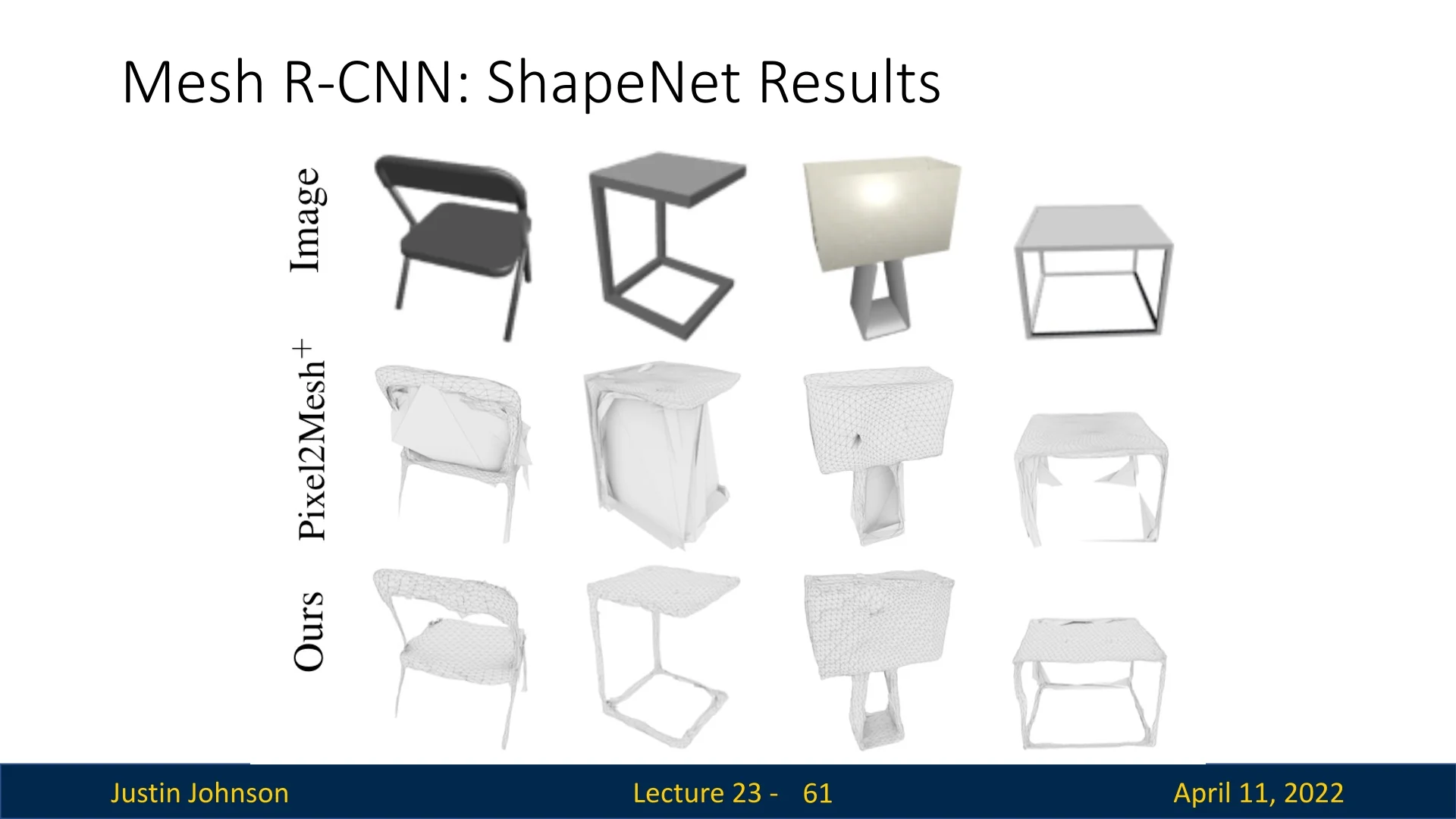
Key Results on Pix3D On real-world scenes, Mesh R-CNN outperforms all baselines (Voxel-Only, Sphere-Init, Pixel2Mesh+) in AP\(_\mbox{mesh}\) across nearly all object categories. Performance gains are especially notable for topologically complex classes like bookcases (+21.6%), tables (+16.7%), and chairs (+7.3%).
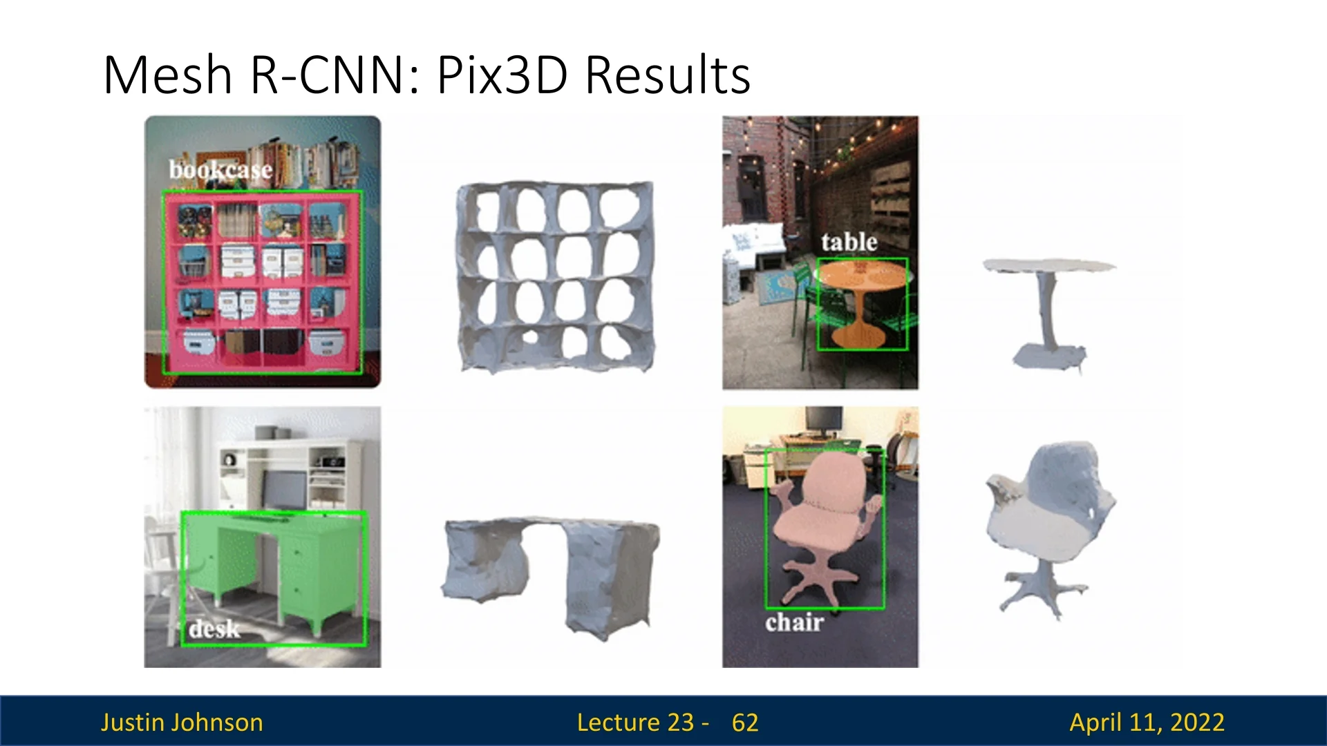
Amodal Completion Mesh R-CNN is capable of completing occluded object geometry. As shown in the following figure, it reconstructs sofas occluded by dogs and chairs, enabled by volumetric reasoning and perceptual feature alignment.
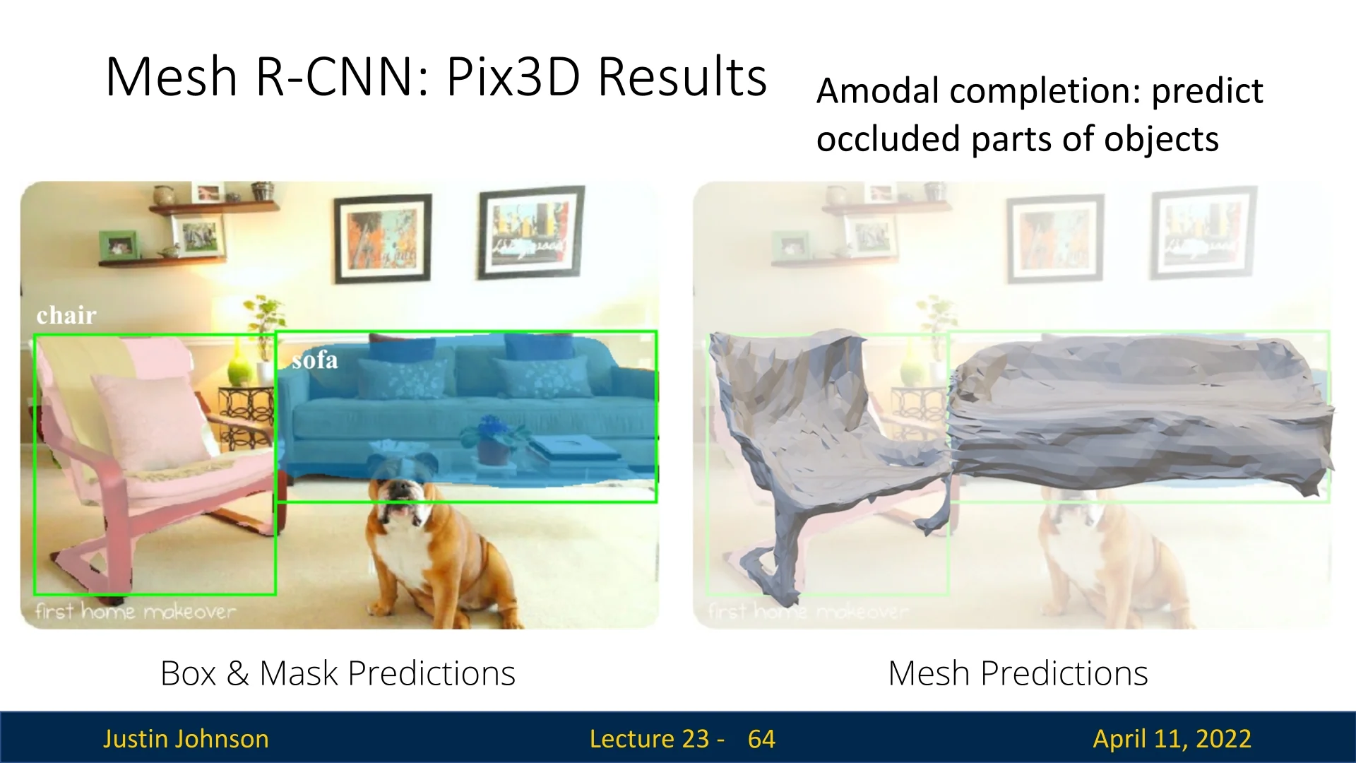
Failure Modes Errors in the 2D segmentation stage can propagate to 3D mesh prediction. The following figure shows a bookshelf with missing compartments due to segmentation holes in the input mask.
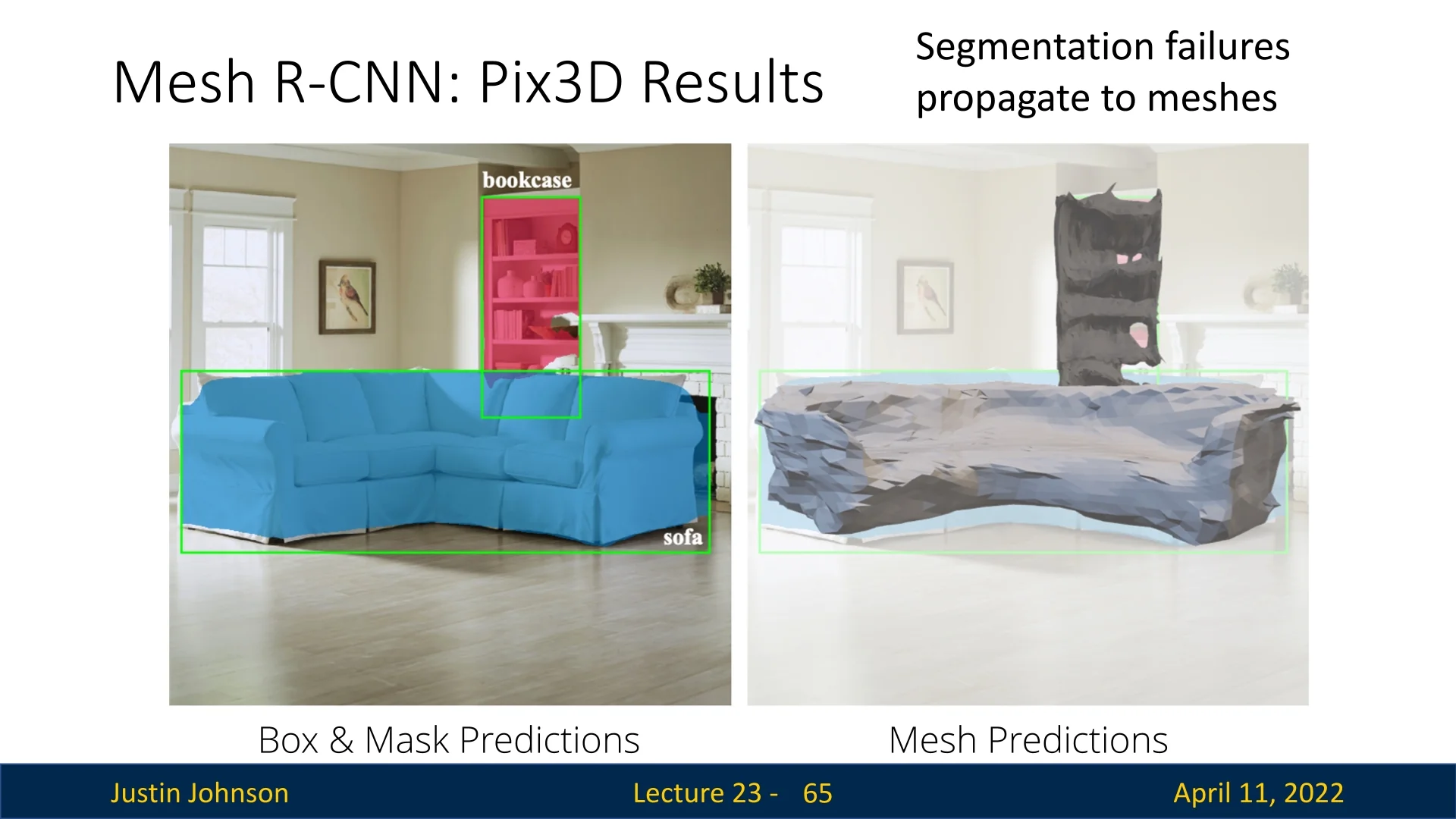
Ablation Studies The performance of Mesh R-CNN is validated through ablation studies that isolate the impact of each architectural and supervisory component. These experiments, conducted on ShapeNet and Pix3D, quantitatively and qualitatively demonstrate why voxel-based initialization, iterative refinement, and geometric regularization are all essential for high-fidelity mesh prediction.
- Voxel-Only: In this setting, the mesh refinement branch is removed and the final mesh is directly obtained via cubify on the voxel occupancy grid. While this preserves coarse topology, the resulting meshes are blocky and lack fine detail. On ShapeNet, the voxel-only model yields a Chamfer distance of \( \mathbf {0.916} \) and an F1@0.3 score of \( \mathbf {33.1\%} \), significantly worse than the full model’s \( \mathbf {0.133} \) Chamfer and \( \mathbf {86.6\%} \) F1@0.3 [183, Table 2]. Similarly, on Pix3D, voxel-only achieves an AP\(_\mbox{mesh}\) of only \( \mathbf {5.3\%} \) vs. \( \mathbf {51.1\%} \) for the full system (Stage 1, COCO pretraining). These results confirm that the voxel branch alone is insufficient for detailed surface recovery; mesh refinement is indispensable.
-
Pixel2Mesh+ and Sphere-Init: These baselines deform a fixed-topology template mesh (typically a genus-0 sphere) using GCN layers. While adequate for simple shapes, they cannot represent objects with holes or disconnected parts. On ShapeNet’s “Holes Test Set,” Pixel2Mesh+ achieves a Chamfer distance of \( \mathbf {0.137} \) and F1@0.3 of \( \mathbf {85.5\%} \), underperforming Mesh R-CNN’s \( \mathbf {0.130} \) and \( \mathbf {86.7\%} \) respectively [183, Table 2]. The performance gap is especially pronounced on Pix3D, where Mesh R-CNN achieves an AP\(_\mbox{mesh}\) of \(48.2\%\) on chairs and \(70.2\%\) on bookcases in Stage 1, compared to \(26.7\%\) and \(34.1\%\) respectively for Pixel2Mesh+, yielding substantial improvements of \(+21.5\%\) and \(+36.1\%\). These results underscore the limitations of fixed-topology deformation approaches and demonstrate the superiority of Mesh R-CNN’s voxel-initialized pipeline, which enables prediction of meshes with arbitrary topology, better aligned to the structural diversity present in real-world images.
- Refinement Stages: Mesh R-CNN performs mesh refinement in three sequential stages, each consisting of vertex-image alignment, graph convolution, and vertex updates. This coarse-to-fine process allows the model to progressively capture global structure and fine surface detail. While the ShapeNet Chamfer distance for the full model with three stages is \( \mathbf {0.133} \) [183, Table 2], the paper does not report direct Chamfer values for single- or two-stage variants on ShapeNet. However, a related ablation on Pix3D reveals that reducing from three to one refinement step degrades AP\(_\mbox{mesh}\) from \( \mathbf {51.1\%} \) to \( \mathbf {48.6\%} \) [183, Table 4]. This validates the benefit of iterative refinement. Although Mesh R-CNN does not visualize per-stage refinement qualitatively, earlier works like Pixel2Mesh show clear improvements in surface smoothness and structure across multiple GCN blocks [686, Figure 6], supporting the intuition that repeated refinement is essential for accurate and detailed reconstructions.
- Loss Term Importance: The edge length regularization loss \( \mathcal {L}_{\mbox{edge}} \) plays a crucial role in ensuring mesh plausibility and geometric stability. While minimizing Chamfer distance alone may improve quantitative alignment, it can produce structurally degenerate results. Mesh R-CNN explicitly demonstrates this tradeoff: removing edge regularization (i.e., setting \( \lambda _{\mbox{edge}} = 0 \)) yields a lower Chamfer distance of \( \mathbf {0.133} \) for the “Best” model on ShapeNet, whereas including it with \( \lambda _{\mbox{edge}} = 0.2 \) in the “Pretty” model increases Chamfer distance to \( \mathbf {0.171} \) [183, Table 2]. However, this quantitative gain comes at the cost of mesh quality. As visually shown in Figure 5, the absence of edge regularization leads to self-intersecting, overlapping faces and triangle clumping [183, Figure 5]. On Pix3D, the “Pretty” model uses a stronger regularization weight \( \lambda _{\mbox{edge}} = 1.0 \), which helps preserve surface coherence and avoid mesh collapse in cluttered scenes. These results, along with similar findings in prior work such as Wang et al. [686, Figure 5], confirm that while edge regularization may reduce agreement with point-based metrics, it is essential for producing visually plausible and topologically stable meshes.
Conclusion These experiments demonstrate that Mesh R-CNN overcomes the limitations of fixed-topology methods by enabling variable-topology meshes, robust 3D inference from cluttered scenes, and end-to-end optimization of 2D and 3D objectives.
23.7 Implicit Surface Representations
From Discrete to Continuous Geometry Traditional 3D shape representations—such as voxel grids, point clouds, or triangle meshes—explicitly enumerate spatial elements. In contrast, implicit surface representations define a shape as the level set of a continuous function \( f : \mathbb {R}^3 \to {0, 1} \). Given any spatial coordinate \( \mathbf {x} \in \mathbb {R}^3 \), the function \( f(\mathbf {x}) \) determines whether the point lies inside, outside, or on the object’s surface. The surface is then implicitly defined as the set \( \{ \mathbf {x} \mid f(\mathbf {x}) = \tau \} \), where \( \tau \) is a fixed threshold—typically \( \tau = 0 \) for signed distance fields or \( \tau = 0.5 \) for occupancy fields.
Occupancy Fields vs. Signed Distance Functions Two widely used formulations of \( f \) are:
- Occupancy Function: Models the probability that a point is inside the object. The function \( f(\mathbf {x}) \in [0,1] \) outputs a probability, and the surface is implicitly defined by the decision boundary \( \{ \mathbf {x} \mid f(\mathbf {x}) = 0.5 \} \).
- Signed Distance Function (SDF): Outputs the signed Euclidean distance from point \( \mathbf {x} \) to the nearest surface. The sign indicates whether the point is inside (negative) or outside (positive), and the surface is given by the zero-level set \( \{ \mathbf {x} \mid f(\mathbf {x}) = 0 \} \).
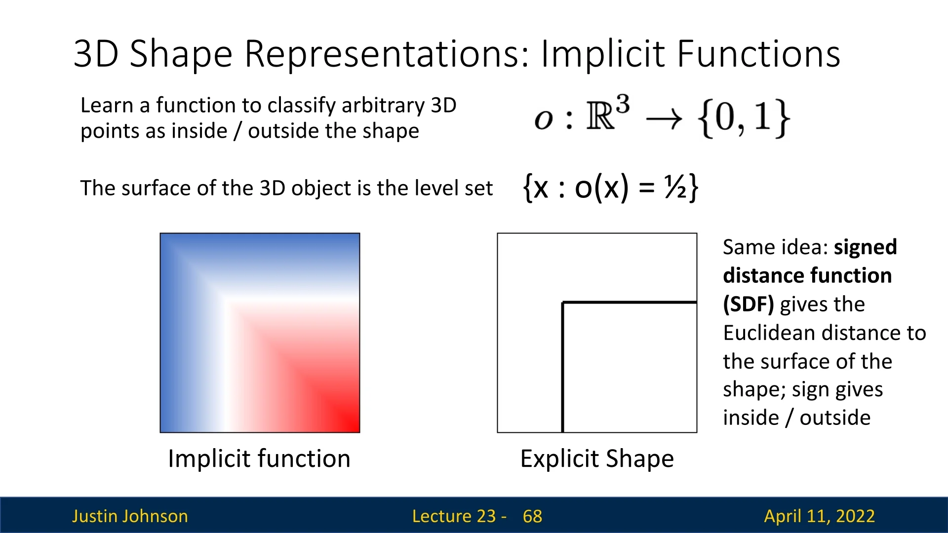
Neural Implicit Models Modern methods represent the function \( f \) using a small multi-layer perceptron (MLP), which maps 3D coordinates \( \mathbf {x} \in \mathbb {R}^3 \) to scalar values indicating occupancy or distance. This neural network can be evaluated at arbitrary resolutions and enables high-fidelity shape representation with a compact memory footprint. Notable examples include Occupancy Networks [437] and DeepSDF [481], both of which learn shape fields by regressing values pointwise.
Why Surface Extraction Is Required Although neural implicit models are continuous and memory-efficient, they do not produce an explicit mesh directly. Most downstream tasks—such as rendering, simulation, or surface loss computation—require a triangulated mesh as output. This motivates dedicated extraction procedures that convert the learned function \( f \) into an explicit surface. The next subsection introduces one such method: Multi-Scale Iso-surface Extraction (MISE), which constructs a mesh by progressively refining a voxel grid where the level set \( f(\mathbf {x}) = \tau \) intersects.
23.7.1 Multi-Scale IsoSurface Extraction (MISE)
Occupancy Networks represent 3D geometry not as explicit meshes or voxels, but as the decision boundary of a learned implicit function \( f_\theta (\mathbf {p}, \mathbf {x}) \). Here, \( \mathbf {p} \in \mathbb {R}^3 \) is a spatial query point, and \( \mathbf {x} \) is a conditioning input (e.g., an image or latent vector). The function predicts whether \( \mathbf {p} \) lies inside the object depicted by \( \mathbf {x} \), typically using a threshold \( \tau = 0.5 \) to define the surface. To extract an explicit mesh from this continuous field, Occupancy Networks use the Multiresolution IsoSurface Extraction (MISE) algorithm [437], which adaptively refines a voxel grid around the surface and outputs a high-resolution mesh.
- Step 1
- Coarse Grid Initialization: To locate the surface approximately, MISE first defines a coarse 3D voxel grid (e.g., \(32^3\)) that spans the object’s bounding box. The occupancy network \( f_\theta (\mathbf {p}, \mathbf {x}) \) is evaluated at each corner of the grid. Voxels whose corners straddle the threshold \( \tau \)—i.e., some values are above and some below—are marked active, since the surface likely intersects them. This step efficiently identifies the region of interest without exhaustively evaluating the entire volume.
- Step 2
- Octree Subdivision: Instead of densely refining the whole grid, MISE recursively subdivides only the active voxels into eight subvoxels (octree refinement). New corner points introduced by the subdivision are evaluated by \( f_\theta \), and voxels are again checked for surface crossings. This process is repeated for \( N \) levels. The result is a spatial hierarchy that is fine near the implicit surface and coarse elsewhere, reducing computation and memory without sacrificing detail.
- Step 3
- Marching Cubes Extraction: Once the highest refinement level is reached, the Marching Cubes algorithm [403] is applied to the final voxel grid. Each voxel’s eight occupancy values define a binary pattern (inside vs. outside), used to index a precomputed triangulation lookup table. Triangles are placed within the voxel by interpolating along edges where occupancy transitions across \( \tau \). Assembled over the full grid, this produces a watertight, manifold mesh approximating the surface.
- Step 4
- Mesh Refinement via Gradient Descent: The initial mesh may lie slightly off the true surface due to grid discretization. To correct this, each vertex \( \mathbf {v} \in \mathcal {V} \) is optimized using gradient descent to minimize the loss \[ \mathcal {L}_{\mbox{align}} = \sum _{\mathbf {v} \in \mathcal {V}} \left ( f_\theta (\mathbf {v}, \mathbf {x}) - \tau \right )^2. \] The gradient \( \nabla _{\mathbf {v}} f_\theta (\mathbf {v}, \mathbf {x}) \) guides each vertex toward the level set \( f_\theta = \tau \), effectively “snapping” the mesh onto the continuous surface. This removes stair-step artifacts and enhances surface fidelity.
Each step in MISE builds upon the last: the coarse grid identifies candidate surface regions; octree subdivision focuses resolution near the surface; Marching Cubes generates an explicit triangle mesh; and gradient refinement polishes the mesh using the implicit signal. The result is a high-resolution, watertight mesh faithful to the learned 3D shape.
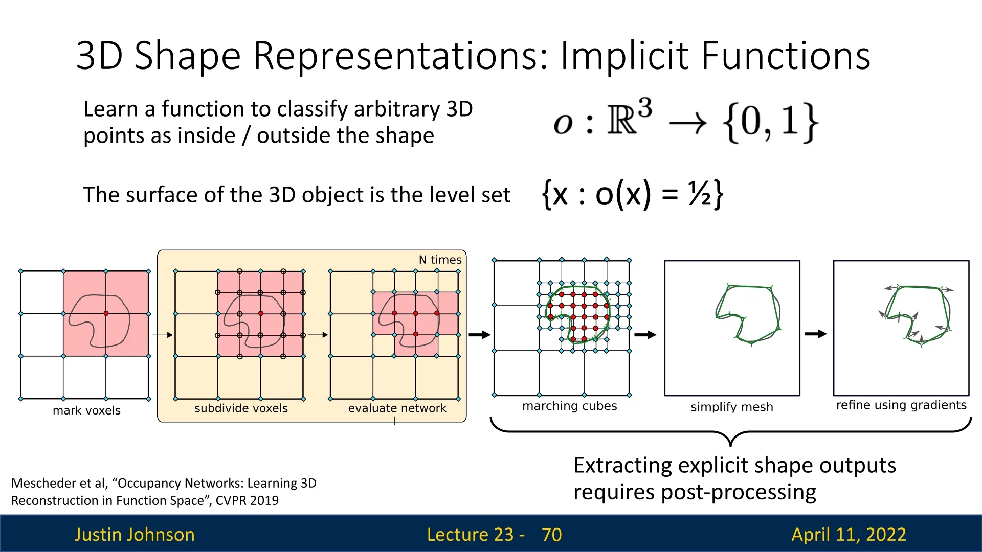
23.7.2 Implicit Surface Advantages & Limitations
Advantages Implicit surface representations offer several key benefits:
- Resolution Independence: Surfaces can be reconstructed at arbitrary resolution with no cubic memory growth.
- Topological Flexibility: No constraints on the number of components, holes, or genus of the reconstructed surface.
- Differentiability: Enables accurate normals, gradient-based surface optimization, and differentiable rendering.
Limitations Despite their flexibility, implicit methods have drawbacks:
- Post-Processing Required: Explicit mesh output demands surface extraction, often involving non-differentiable Marching Cubes or costly optimization.
- Slow Evaluation: Each point query requires a forward pass through the network; querying millions of points is expensive.
- Supervision Demands: High-quality training requires accurate surface-level supervision, often obtained from watertight CAD models.
Relation to Octrees and Voxel Refinement As in Octree Generating Networks (OGNs), implicit representations benefit from adaptive subdivision. Unlike OGNs, however, implicit models do not need to explicitly store voxel contents—pointwise evaluation suffices. This makes them ideal for continuous or parametric 3D learning pipelines.
23.8 General 3D Topics
This section outlines three foundational aspects relevant across most 3D reconstruction pipelines: metrics for shape comparison, the choice of coordinate systems, and the major datasets used for training and evaluation. Understanding these design decisions is critical for interpreting model performance and selecting the right tools for the task at hand.
23.8.1 Shape Comparison Metrics
Voxel IoU: Intuitive but Limited In 2D image tasks, metrics like Intersection-over-Union (IoU) for bounding boxes and segmentation masks are widely used. A natural idea is to extend IoU to 3D by voxelizing the shape and comparing binary occupancy grids. However, this introduces several issues, as discussed by Tatarchenko et al. [631]:
- Loss of fine structures: Thin parts (e.g., table legs or airplane wings) may disappear when voxelized at coarse resolutions.
- Representation mismatch: Point clouds and meshes must be rasterized to voxels, introducing approximation error.
- Metric collapse: At low overlap, IoU scores saturate near zero and fail to distinguish plausible from implausible reconstructions.
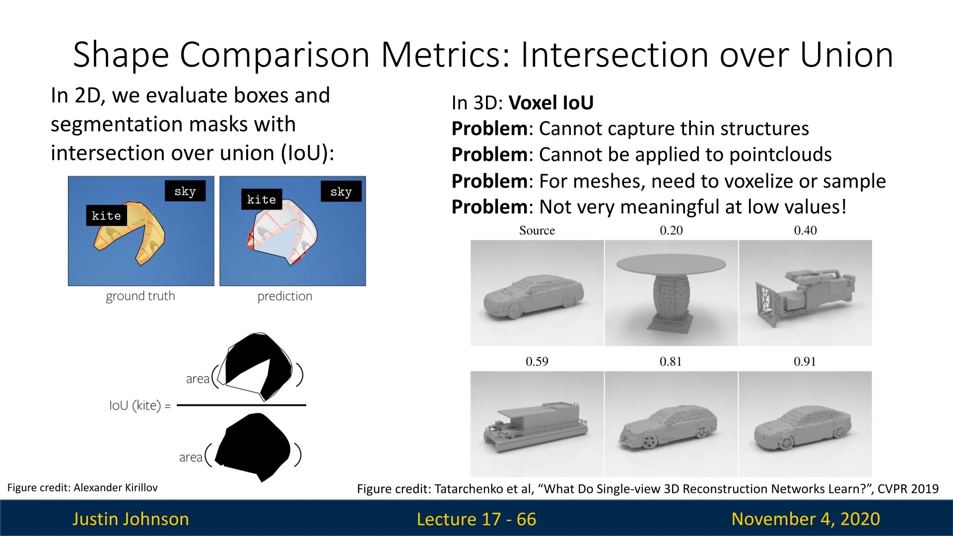
Chamfer Distance: Simple and Effective A widely adopted alternative is the Chamfer distance (CD), which compares two point clouds by computing nearest-neighbor distances in both directions:
\[ \mbox{CD}(P, Q) = \frac {1}{|P|} \sum _{p \in P} \min _{q \in Q} \|p - q\|_2^2 + \frac {1}{|Q|} \sum _{q \in Q} \min _{p \in P} \|q - p\|_2^2. \]
CD works well for arbitrary 3D representations and is differentiable, making it a common loss function. However, it is highly sensitive to outliers due to its reliance on squared \( \ell _2 \) distances.
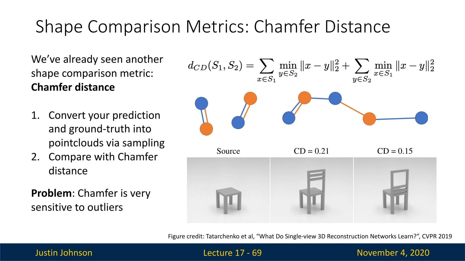
F1 Score: Thresholded Surface Accuracy To address CD’s sensitivity, we can compute precision and recall over thresholded nearest-neighbor distances:
- Precision@\(t\): Fraction of predicted points within distance \(t\) of the ground-truth surface.
- Recall@\(t\): Fraction of ground-truth points within distance \(t\) of the prediction.
- F1@\(t\): Harmonic mean: \( \displaystyle \frac {2 \cdot \mbox{Precision@}t \cdot \mbox{Recall@}t}{\mbox{Precision@}t + \mbox{Recall@}t} \)
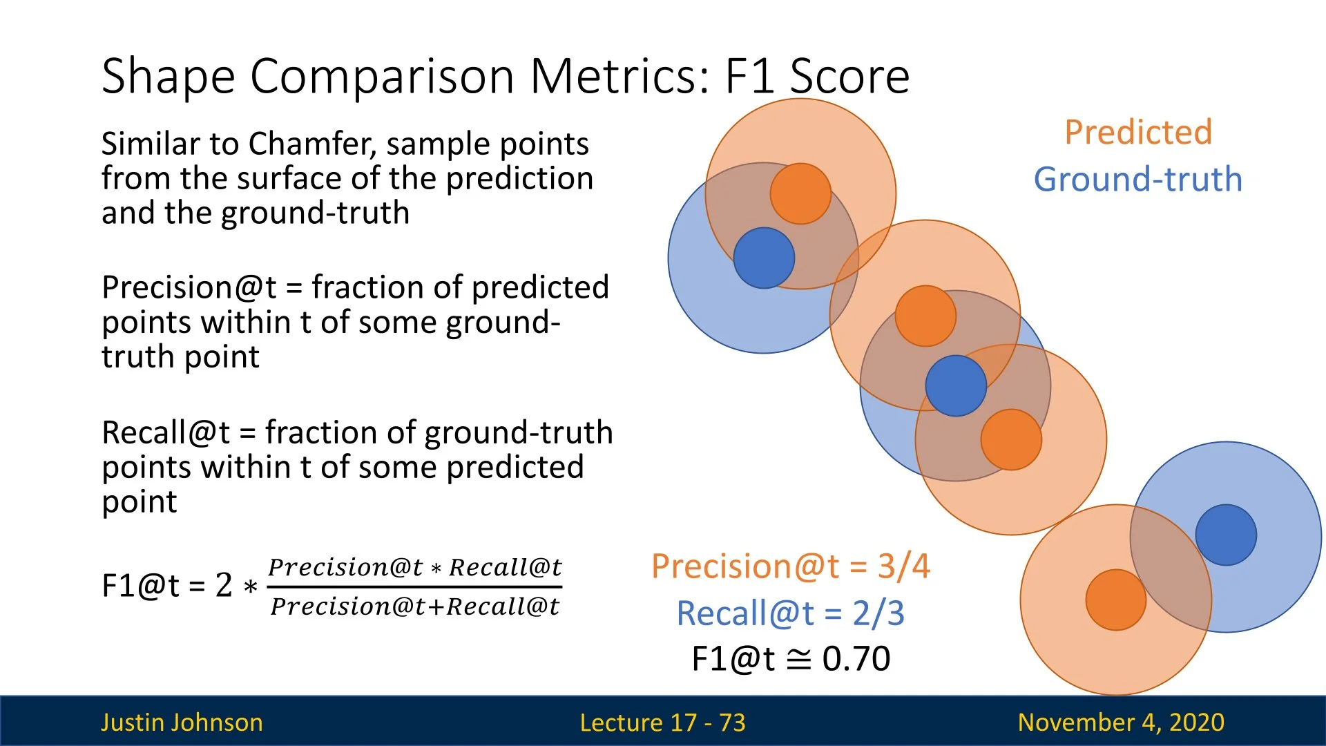
Threshold Sensitivity F1@\(t\) is only meaningful at the right spatial scale. Too small a \(t\) penalizes fine misalignments; too large a \(t\) washes out detail. Therefore, it is standard practice to report F1@\(t\) for multiple values of \(t\).
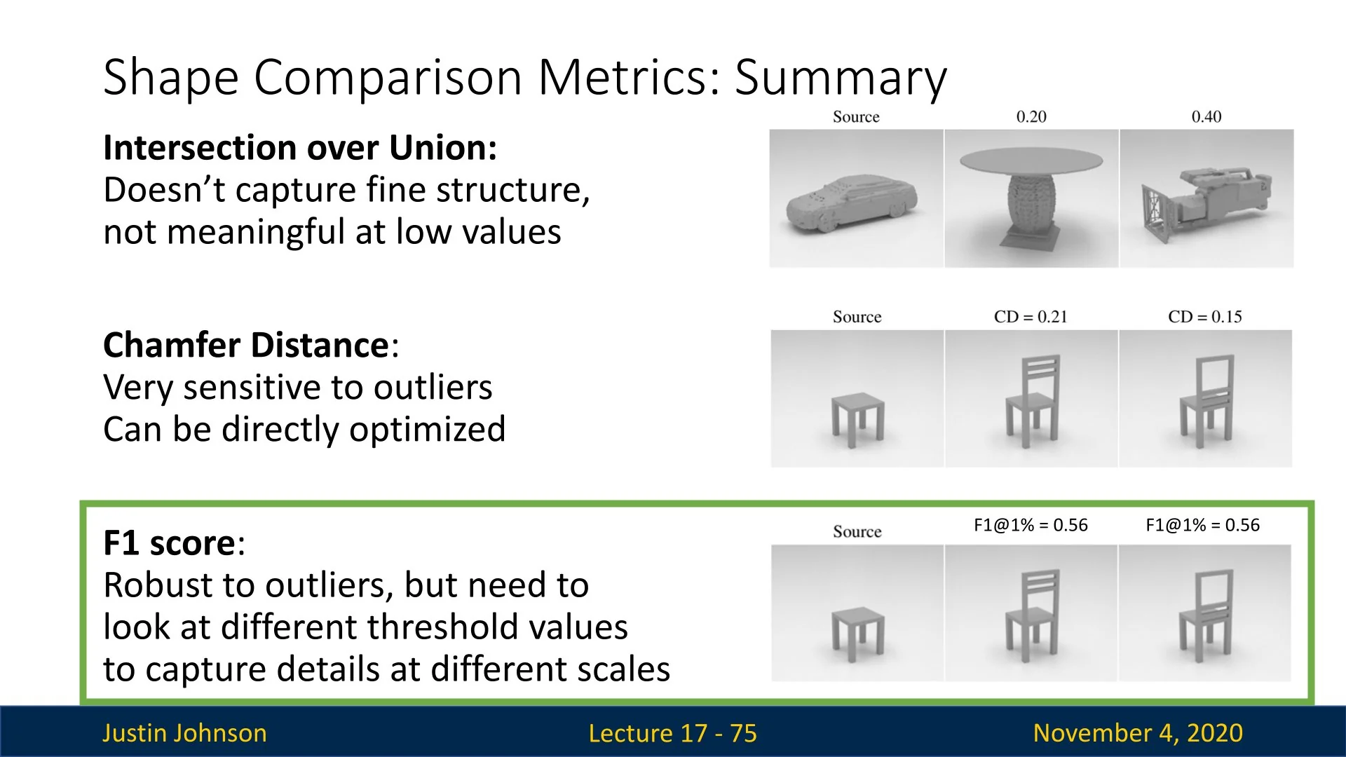
23.8.2 Camera Coordinates: Canonical vs. View-Aligned
Canonical Coordinates Many 3D pipelines predict objects in a canonical orientation (e.g., front of chair = \(+z\)), which simplifies training and dataset organization. However, this introduces a disconnect between the input viewpoint and the output geometry, forcing the model to learn pose estimation as a side task.
View Coordinates Alternatively, we can predict shapes aligned with the input camera pose. This simplifies feature alignment and improves generalization. The 2018 CVPR study by Shin et al. [585] demonstrates that view-coordinates lead to better results on novel objects and unseen categories.
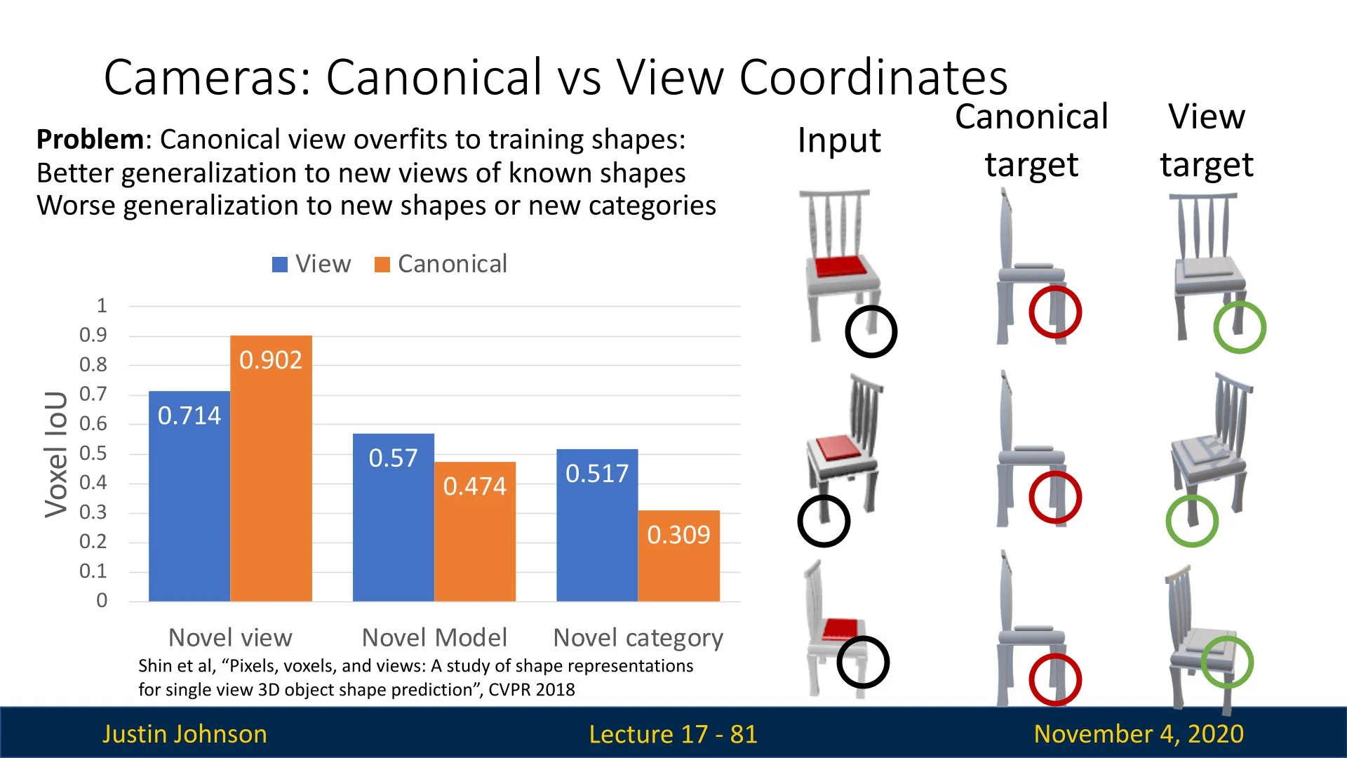
Conclusion Unless a downstream task requires a fixed coordinate frame (e.g., assembly simulation), predicting in view coordinates is preferred due to its alignment benefits and superior generalization.
23.8.3 3D Datasets
Core Benchmarks for Single-View Reconstruction 3D reconstruction methods typically train and evaluate on a handful of publicly available datasets. The two most influential are ShapeNet and Pix3D, which together define the synthetic-to-real spectrum of object-level benchmarks.
ShapeNet ShapeNet [76] is the dominant synthetic dataset for learning object geometry from images. It provides clean, manifold CAD meshes with consistent alignment and dense annotations.
- Scale: Over 50,000 3D models across 55 categories. The Core v2 split uses 13 categories for benchmarking.
- Images: Each object is rendered from 20–25 uniformly sampled viewpoints on a hemisphere.
- Advantages: Large scale, watertight geometry, and complete surface supervision.
- Limitations: Synthetic only; lacks real lighting, texture variation, or background context. Category distribution is skewed (e.g., chairs dominate).
Pix3D Pix3D [615] bridges synthetic geometry with real-world scenes. It aligns 3D furniture CAD models with natural RGB images of the same object instances, captured in real environments.
- Scale: 219 unique 3D models and 17,000 real images across 9 furniture categories.
- Advantages: Contains lighting variation, clutter, and occlusion; includes ground-truth pose, segmentation, and mesh alignment.
- Limitations: Small object coverage; only one labeled object per image; annotations are sometimes incomplete or noisy.
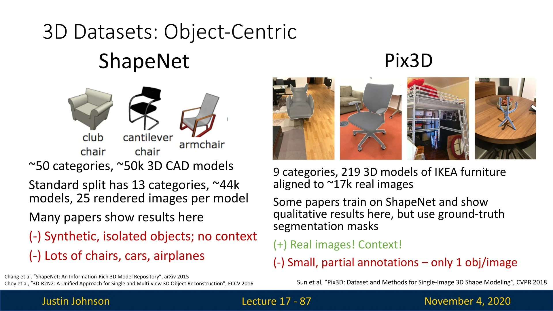
Training Strategy A common pipeline is to pretrain on ShapeNet for geometry learning and fine-tune or evaluate qualitatively on Pix3D to test robustness to clutter, occlusion, and real-world image statistics.
However, as 3D learning expands, modern benchmarks increasingly push beyond these datasets in scale, realism, and diversity.
CO3D: Common Objects in 3D CO3D [537] comprises internet-scale videos of common objects (e.g., bottles, toys, shoes) captured using handheld phones. It includes camera poses and multi-view image sequences.
- Scale: Over 1.5 million frames from 50 categories; hundreds of object instances per class.
- Use Case: Training category-specific NeRFs and multi-view consistent models.
- Strengths: Real-world occlusion and lighting; dense image-based supervision.
Objaverse and Objaverse-XL Objaverse [118] is a web-scale dataset of Creative Commons–licensed 3D assets, released to support foundational 3D vision models and text–3D learning.
- Scale: 10M+ meshes across a wide spectrum of categories; many include textures and captions.
- Use Case: Pretraining CLIP-style vision–language–geometry models.
- Strengths: Unprecedented diversity and licensing openness; extensible for 3D GenAI.
- Challenges: Inconsistent mesh quality and scaling; preprocessing required.
ScanNet ScanNet [115] provides RGB-D video scans of real-world indoor scenes with semantic and instance segmentation labels.
- Scale: 1,500 scans and over 2.5 million RGB-D frames.
- Use Case: Scene-level 3D understanding, SLAM, and real-world domain generalization.
- Strengths: Photorealism, full-scene context, dense camera trajectories.
- Limitations: No watertight ground-truth meshes; reconstructed via noisy TSDF fusion.
Supplementary Datasets While most reconstruction benchmarks focus on visual realism, other datasets support tasks like analytic surface modeling or object detection.
- ABC Dataset [312]: 1M parametric CAD models in STEP format, designed for curvature estimation and surface fitting. Rich in metadata but lacks textures and everyday context.
- ModelNet [728]: 12k CAD meshes across 10 or 40 categories. Still common in point cloud classification; now largely superseded by ShapeNet.
- PartNet [452]: Over 26k 3D models with fine-grained, hierarchical part annotations—useful for segmentation and affordance tasks.
- Objectron [2]: Short AR videos with annotated 3D bounding boxes for 15 object categories. Captures real-world scale and motion but only provides sparse 3D annotations.
Summary ShapeNet and Pix3D remain the standard benchmarks for mesh-level shape prediction. Newer datasets like CO3D and Objaverse expand the task to multi-view learning and massive-scale generalization. Scene-level datasets like ScanNet and industrial corpora like ABC enable new frontiers in physical realism, structure, and simulation fidelity. A robust training curriculum typically begins with synthetic pretraining and proceeds to real-world fine-tuning.
23.9 Neural Radiance Fields (NeRF)
23.9.1 Problem Setup: Novel View Synthesis with Known Cameras
What Is Novel View Synthesis? Imagine taking several photos of a scene—say, a Lego bulldozer—from different known positions. Now imagine rendering a new image of that same scene from a viewpoint you never captured. This task is called novel view synthesis: the goal is to generate realistic images of a scene as it would appear from arbitrary camera positions, given only a sparse set of observed images and their corresponding camera poses. This problem sits at the intersection of geometry, appearance modeling, and rendering—and is central to applications in virtual reality, 3D reconstruction, and photorealistic simulation.
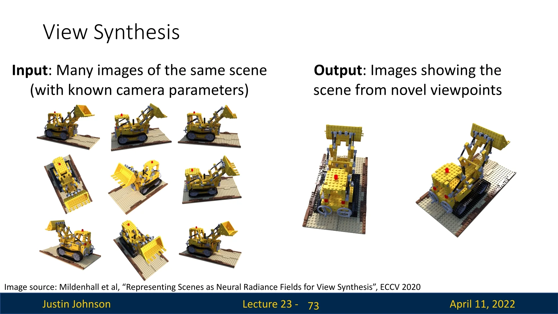
Limitations of Traditional Novel View Synthesis Pipelines Classical novel view synthesis systems follow a brittle, multi-stage pipeline rooted in explicit 3D reconstruction [576, 793, 571]:
- Structure-from-Motion (SfM). Estimates camera intrinsics and extrinsics by matching 2D features across views and triangulating sparse 3D keypoints.
- Multi-View Stereo (MVS). Densifies the sparse point cloud using stereo correspondence and depth estimation across calibrated views.
- Surface reconstruction and texturing. Generates a mesh or voxel grid and back-projects color information from input images to produce a renderable surface.
This pipeline is highly sensitive to noise. The explicit geometry produced in early stages must support all downstream tasks; any errors in pose estimation, depth prediction, or surface reconstruction propagate without correction.
In practice, these systems frequently fail due to several structural limitations:
- Limited view coverage. Geometry is only recovered where multiple views overlap. Occluded or unobserved regions remain incomplete or hallucinated [576].
- Photometric assumptions. Most SfM–MVS methods assume Lambertian surfaces and brightness constancy. Real-world effects such as specularities, translucency, and variable illumination violate these assumptions, corrupting correspondence and depth estimates .
- Sparse inputs and wide baselines. With few input images or large viewpoint shifts, feature correspondences become unreliable, degrading both pose and geometry [1].
- Textureless or repetitive regions. Surfaces lacking distinctive features—e.g., white walls—or containing repeated patterns confuse matching algorithms, leading to holes or incorrect geometry [793].
- Error accumulation and memory cost. Small mismatches, pose drift, and meshing artifacts accumulate through the pipeline. High-resolution volumetric grids also incur steep memory and computational costs [576].
Moreover, traditional methods commit to a single explicit surface. Modeling view-dependent phenomena (e.g., reflections, specular highlights) requires hand-designed reflectance functions (e.g., BRDFs) that are difficult to estimate and rarely generalize across real-world conditions.
Neural Radiance Fields (NeRF) [442, 378] were introduced to overcome these fragilities. Rather than reconstructing a discrete surface, NeRF learns a continuous, view-conditioned radiance field from posed images. Novel views are rendered directly by integrating this field along camera rays via differentiable volume rendering—yielding sharper, more consistent results even under challenging visibility, appearance, and lighting conditions.
23.9.2 A New Paradigm: Neural Fields
Neural Radiance Fields (NeRF) [442] exemplify a transformative shift in view synthesis: from pipelines that reconstruct explicit 3D geometry to models that learn neural fields, also known as implicit neural representations. Rather than discretizing scenes into meshes or voxel grids, neural fields represent continuous volumetric functions using the parameters of a multilayer perceptron (MLP). These functions take spatial coordinates—optionally conditioned on direction—and output physical scene properties such as radiance, density, or occupancy.
Scene Representation In NeRF, the scene is defined by a function \[ F_\Theta : (x, y, z, \theta , \phi ) \mapsto (\sigma , \mathbf {c}) \in \mathbb {R}_{\geq 0} \times [0,1]^3, \] where \((x, y, z)\in \mathbb {R}^3\) denotes a location in world coordinates and \((\theta , \phi )\) specify the viewing direction using spherical coordinates. The output consists of:
- Volume density \(\sigma \): a scalar indicating the probability of light terminating (i.e., hitting material) at the queried point.
- Radiance \(\mathbf {c}\): an RGB value specifying the color emitted from that point in direction \((\theta , \phi )\).
This directional dependence enables the model to capture view-dependent phenomena like specular highlights or reflections.
Why Only Direction Matters Notably, NeRF conditions on the viewing direction rather than the full camera pose. This is because the color emitted at a given location depends only on the relative angle between the viewing ray and the local surface normal—not on the absolute camera orientation. The roll angle (in-plane camera rotation) does not affect light interaction and is therefore omitted from the input.
Training Supervision: From Images to Rays NeRF is trained on a set of images with known camera intrinsics and extrinsics. For each pixel, a corresponding 3D ray is defined using the camera model, and the radiance field is queried along that ray. The goal is to learn \(\Theta \) such that the predicted color along each ray matches the observed pixel value. This requires accurate knowledge of the camera parameters associated with each image in the dataset.
23.9.3 Camera Parameters as a Prerequisite
For NeRF to model and render a scene accurately, it must first understand the relationship between each 2D input image and the shared 3D world coordinate system. This requires, for every image, a complete specification of the camera’s parameters—both internal and external. These parameters form the geometric scaffolding that enables NeRF to associate each pixel with a corresponding 3D ray.
- Intrinsics define the internal projection geometry of the camera and are typically encoded by a \( 3 \times 3 \) calibration matrix \( K_k \) for image \( k \). This matrix specifies the focal lengths \((f_x, f_y)\) and the principal point \((c_x, c_y)\), which together determine how 3D points in camera coordinates are projected onto the 2D image plane: \[ K_k = \begin {bmatrix} f_x & 0 & c_x \\ 0 & f_y & c_y \\ 0 & 0 & 1 \end {bmatrix} \] Optional intrinsics may also include lens distortion parameters, though these are typically omitted or corrected in NeRF datasets.
- Extrinsics define the pose of the camera with respect to a global world coordinate frame. They consist of a rotation matrix \(\mathbf {R}_k\) and a translation vector \(\mathbf {t}_k\) for image \(k\), which together specify a camera-to-world transformation \([\mathbf {R}_k \mid \mathbf {t}_k] \in \mathrm {SE}(3)\). This mapping is essential for expressing 3D locations consistently across all views.
These parameters are crucial because NeRF learns a function over 3D world coordinates. To supervise this function using 2D image pixels, the model must be able to trace each pixel’s ray through the scene—originating from the camera’s position and passing in the direction that pixel subtends in space. Without accurate intrinsics and extrinsics, this mapping from pixel to 3D ray cannot be defined, and the network cannot learn a consistent radiance field.
In practice, these camera parameters are not usually provided with the dataset and must be estimated from the images themselves. Their accuracy is critical: small errors in estimated poses result in misaligned rays, which in turn degrade the consistency of supervision across views. This often leads to blurred reconstructions or ghosting artifacts in rendered images, especially in regions of fine structure or high frequency detail.
Accordingly, before training NeRF, a robust geometric calibration step must be performed to recover per-image intrinsics and extrinsics. The standard approach is to estimate these parameters from the image set itself using classical techniques based on multi-view geometry.
Recovering Camera Parameters via SfM As previously mentioned, in most real-world datasets, explicit camera parameters are not available. To bridge this gap, NeRF typically relies on classical Structure-from-Motion (SfM) [571] pipelines to estimate both intrinsic and extrinsic parameters directly from the image collection. This process aligns the entire dataset into a unified 3D coordinate frame and enables ray construction for NeRF training.
SfM recovers this calibration through the following multi-stage optimization:
- 1.
- Feature correspondence: Local image features (e.g., SIFT) are detected and matched across image pairs to establish 2D correspondences—keypoints that observe the same 3D point across views.
- 2.
- Triangulation: Using matched keypoints and camera projection geometry, 3D point locations are triangulated, resulting in a sparse point cloud that defines the underlying scene structure.
- 3.
- Bundle adjustment: A global nonlinear optimization jointly refines all estimated camera parameters and 3D points by minimizing reprojection error. This adjusts the intrinsics, extrinsics, and 3D structure to best explain the observed 2D matches across the dataset.
The result is a calibrated camera model for each image, typically consisting of a pose \( \mathcal {P}_k = (\mathbf {R}_k, \mathbf {t}_k) \in \mathrm {SE}(3) \) and an intrinsics matrix \( K_k \). Together, these determine the origin and direction of every ray traced from pixel to world, anchoring the supervision of NeRF’s radiance field.
However, SfM is not infallible. Challenging image regions—such as occlusions, textureless surfaces, or large baselines—can lead to pose drift and imperfect alignments. These miscalibrations cause ray inconsistencies across views and may lead to visual artifacts such as ghosting or blur. To address this, many NeRF variants treat the poses as learnable parameters and jointly optimize them alongside the radiance field, refining camera geometry in tandem with appearance modeling.
With camera calibration complete, each pixel in each training image defines a 3D ray in world space. The next stage is to evaluate the neural radiance field along these rays using differentiable volume rendering.
23.9.4 Volume Rendering: From Rays to Pixels
Once calibrated rays are constructed from the camera intrinsics and extrinsics, the NeRF pipeline proceeds to synthesize pixel colors by simulating how light accumulates along each ray. This is achieved through a process known as volume rendering, a classical technique from graphics that models a ray traversing a semi-transparent scene.
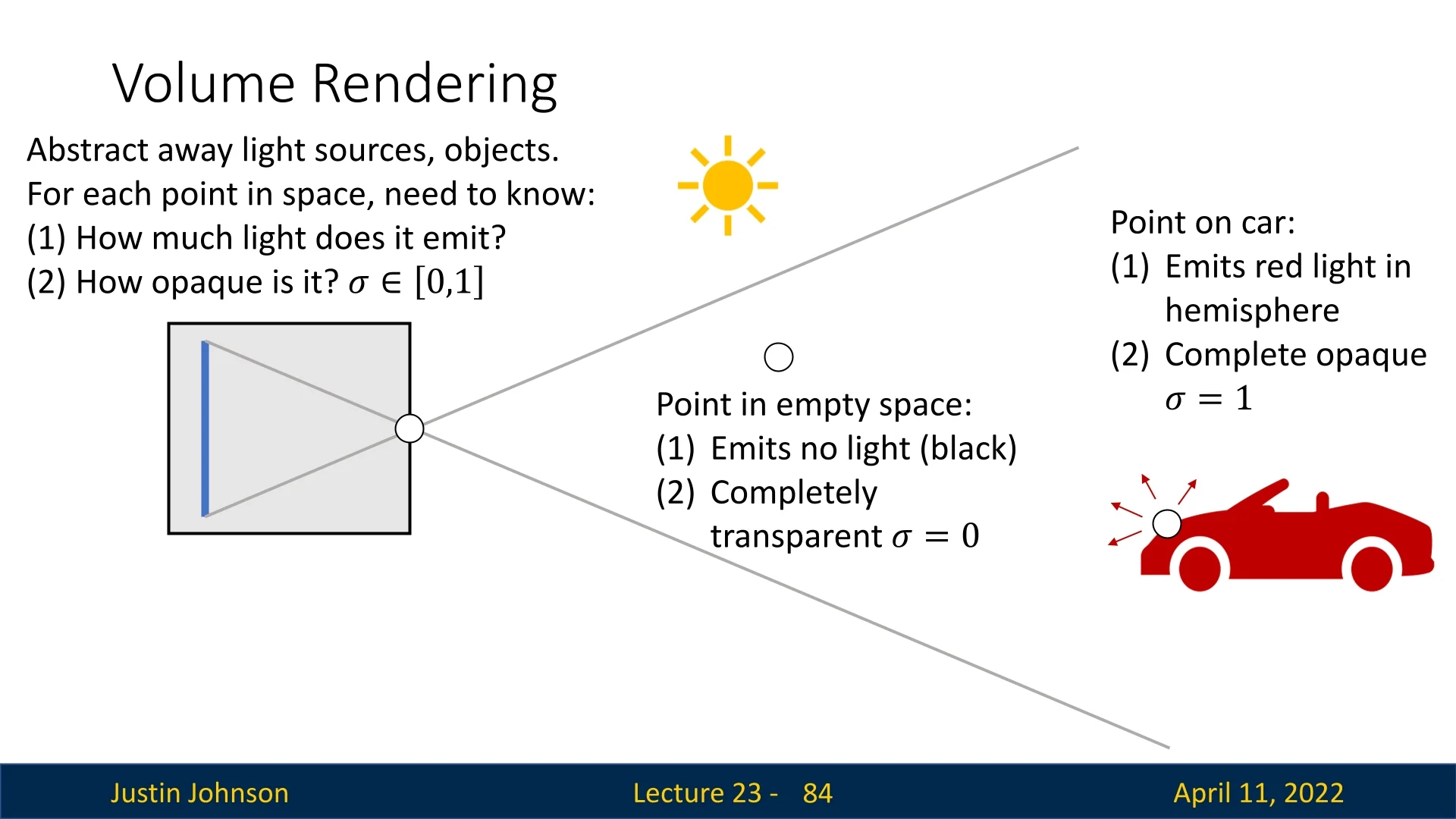
To determine the color of a single pixel, NeRF casts a ray from the camera’s optical center into the 3D scene, simulating how light accumulates along that path. Under the pinhole camera model, every ray originates from a single 3D point—the camera center—and passes through a specific location on the image plane. This ray is parameterized as: \[ \mathbf {r}(t) = \mathbf {o} + t\mathbf {d}, \quad t \in [t_n, t_f], \] where:
- \( \mathbf {o} \in \mathbb {R}^3 \) is the ray origin in world coordinates. It corresponds to the physical center of projection—the point through which all rays pass—and is computed for image \( k \) from its extrinsics: \[ \mathbf {o}_k = -\mathbf {R}_k^\top \mathbf {t}_k. \] This expression inverts the camera pose transformation \( [\mathbf {R}_k \mid \mathbf {t}_k] \), yielding the camera’s location in the global coordinate frame.
- \( \mathbf {d} \in \mathbb {S}^2 \) is the unit direction vector that points from the camera center \( \mathbf {o} \) through the center of pixel \( (u, v) \) on the image plane. It is carefully constructed so that the ray intersects the sub-pixel center of the target pixel, ensuring accurate alignment and avoiding aliasing artifacts.
To compute \( \mathbf {d} \), NeRF inverts the pinhole projection model in three steps:
- 1.
- Target the pixel center: Pixels are indexed by integer raster coordinates \( (u, v) \in \mathbb {Z}^2 \), which reference their top-left corners. To model light paths more precisely, NeRF offsets these coordinates by \( +\tfrac {1}{2} \), aiming the ray through the center of the square pixel: \[ \mathbf {p}_{\mbox{pix}} = \begin {bmatrix} u + \tfrac {1}{2} \\ v + \tfrac {1}{2} \\ 1 \end {bmatrix}. \] This homogeneous 2D point lies on the image plane and acts as the projected target for the ray.
- 2.
- Unproject to camera space: The camera intrinsics matrix \( K \in \mathbb {R}^{3 \times 3} \), \[ K = \begin {bmatrix} f_x & 0 & c_x \\ 0 & f_y & c_y \\ 0 & 0 & 1 \end {bmatrix}, \] encodes the focal lengths and principal point. Applying the inverse intrinsics yields a direction vector in the camera’s local 3D frame: \[ \mathbf {d}_{\mbox{cam}} = K^{-1} \mathbf {p}_{\mbox{pix}}. \] This vector points from the camera origin through the pixel center, intersecting the virtual image plane at depth \( z = 1 \).
- 3.
- Transform to world space and normalize: To express the ray direction in global coordinates, we rotate the camera-frame direction using the inverse rotation: \[ \mathbf {d}_{\mbox{world}} = \mathbf {R}^\top \mathbf {d}_{\mbox{cam}}, \quad \mathbf {d} = \frac {\mathbf {d}_{\mbox{world}}}{\| \mathbf {d}_{\mbox{world}} \|_2}. \]
The resulting ray \( \mathbf {r}(t) = \mathbf {o} + t\mathbf {d} \) travels through two key points: the camera center \( \mathbf {o} \) and the 3D location that maps—via projection—to the center of pixel \( (u, v) \). This construction ensures that each pixel defines a unique 3D ray that is both photometrically accurate and geometrically aligned.
- \( t \in [t_n, t_f] \) is the depth parameter along the ray. Each value of \( t \) specifies a point \( \mathbf {r}(t) \) in 3D space. The interval bounds the segment of the ray used for rendering: \( t_n \) avoids camera-adjacent voids, and \( t_f \) limits traversal to a relevant portion of the scene.
This setup defines the geometric foundation for NeRF’s differentiable volume rendering pipeline: each pixel gives rise to a calibrated 3D ray that queries the scene via learned color and density functions, enabling accurate supervision from multiview imagery.
The color of a pixel is modeled as a continuous accumulation of radiance along its viewing ray: \[ \mathcal {C}(\mathbf {r}) = \int _{t_n}^{t_f} \underbrace {T(t)}_{\mbox{transmittance}} \cdot \underbrace {\sigma (\mathbf {r}(t))}_{\mbox{density}} \cdot \underbrace {\mathbf {c}(\mathbf {r}(t), \mathbf {d})}_{\mbox{radiance}} \, dt. \] This integral aggregates light contributions from all points \( \mathbf {r}(t) \) along the ray segment between a near bound \( t_n \) and far bound \( t_f \). At each infinitesimal location, the integrand quantifies how much light is emitted, how much material is present, and how likely that light is to reach the camera unoccluded.
- The volume density \( \sigma (\mathbf {r}(t)) \in [0,1] \) acts as a soft occupancy field—higher values indicate denser or more opaque regions, while \( \sigma = 0 \) corresponds to empty space.
- The radiance \( \mathbf {c}(\mathbf {r}(t), \mathbf {d}) \in [0,1]^3 \) gives the RGB color emitted from point \( \mathbf {r}(t) \) in viewing direction \( \mathbf {d} \).
- The transmittance \( T(t) \in [0,1] \) denotes the survival probability of light traveling from the camera to depth \( t \), without being blocked by foreground matter.
Why an integral? Because the scene is modeled as a continuous volumetric field, there is no single surface to sample. Instead, light can originate from anywhere along the ray. Each point emits some color, attenuated by the surrounding medium, and contributes only a tiny amount. The integral sums up these infinitesimal contributions from all depths \( t \in [t_n, t_f] \), forming a composite pixel color. This approach mirrors how light propagates through translucent media in physics and allows smooth transitions, semi-transparent edges, and view-dependent blending.
More precisely, \( \sigma \cdot \mathbf {c} \, dt \) represents the amount of light emitted by a small segment \( dt \) around \( \mathbf {r}(t) \), and \( T(t) \) scales this emission based on how much of it survives traversal through the density field in front of it. The closer the point is to the camera, the less likely it is to be occluded, making early segments contribute more strongly. Distant points can only affect the pixel color if transmittance remains high—i.e., if the path before them is transparent.
The transmittance term is computed as an exponential of the accumulated density: \[ T(t) = \exp \left ( -\int _{t_n}^{t} \sigma (\mathbf {r}(s)) \, ds \right ). \] This expression is a solution to the radiative transfer equation under absorption-only conditions and follows the Beer–Lambert law. It encodes the idea that every unit of density along the path slightly diminishes light transmission. The more material encountered before \( t \), the smaller \( T(t) \) becomes. Thus, occlusion emerges naturally from integration—no hard surfaces or visibility heuristics are needed.
This continuous, differentiable formulation enables NeRF to produce photorealistic renderings with accurate soft shadows, translucency, and gradual occlusion. It replaces discrete surface modeling with an elegant volumetric framework in which geometry and appearance emerge implicitly from learned density and radiance fields.
Discretizing the Rendering Equation: Stratified Sampling and Alpha Compositing Evaluating the continuous integral is analytically intractable for neural fields. NeRF approximates it by sampling \( N \) depths \( t_1, \dots , t_N \) uniformly or via hierarchical importance sampling along the ray. At each sampled point \( \mathbf {r}(t_i) \), the MLP predicts: \[ \sigma _i := \sigma (\mathbf {r}(t_i)), \qquad \mathbf {c}_i := \mathbf {c}(\mathbf {r}(t_i), \mathbf {d}). \]
Assuming that density is constant over the small interval \( [t_i, t_{i+1}] \), we define: \[ \delta _i := t_{i+1} - t_i, \qquad \alpha _i := 1 - \exp (-\sigma _i \delta _i), \] where \( \alpha _i \) approximates the opacity—the probability that the ray terminates inside segment \( i \).
The discrete transmittance \( T_i \) up to segment \( i \) is thus: \[ T_i := \prod _{j=1}^{i-1} (1 - \alpha _j) = \exp \left ( -\sum _{j=1}^{i-1} \sigma _j \delta _j \right ), \] the probability that light successfully traverses all prior segments without being absorbed.
With these components, the rendered pixel color is approximated as: \[ \hat {\mathcal {C}}(\mathbf {r}) = \sum _{i=1}^{N} T_i \cdot \alpha _i \cdot \mathbf {c}_i. \] This rule is mathematically equivalent to front-to-back alpha compositing, where each semi-transparent segment contributes its color, modulated by its own opacity and the transparency of everything in front.
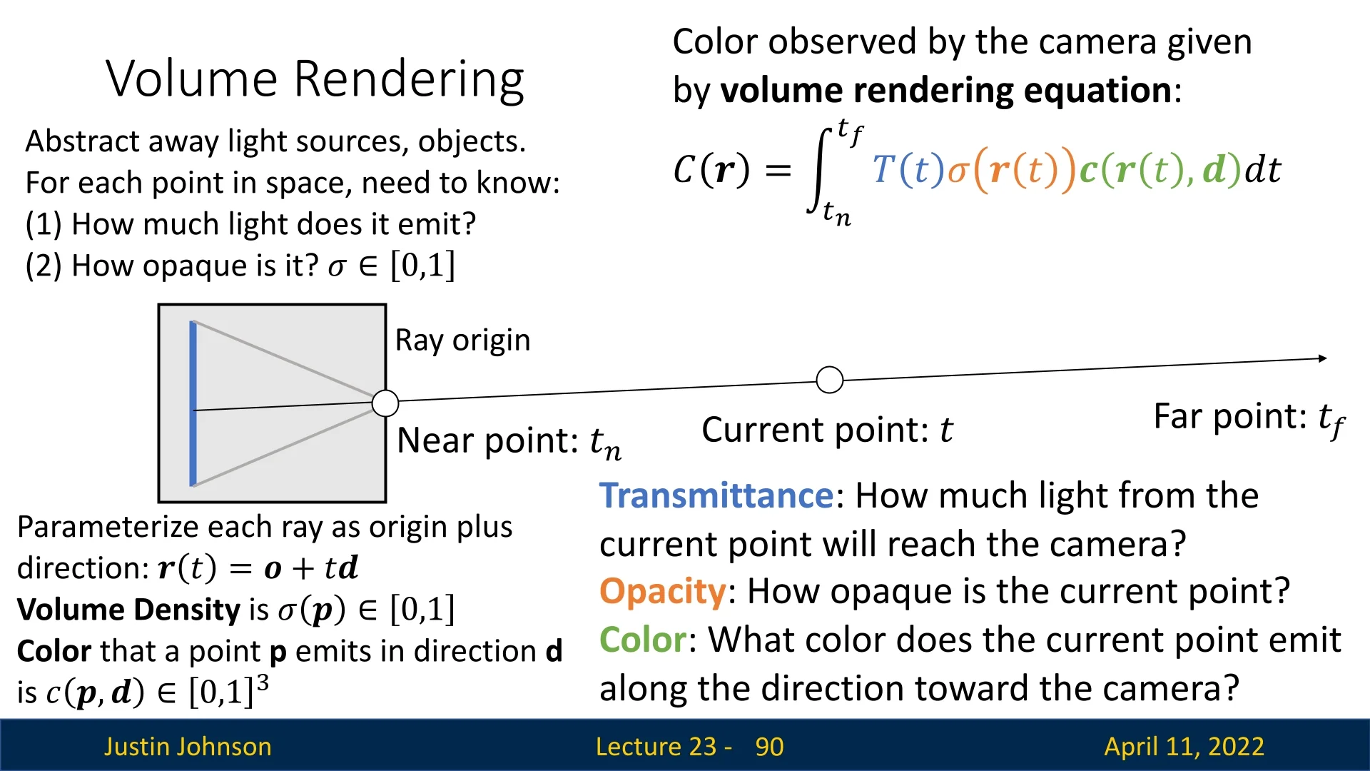
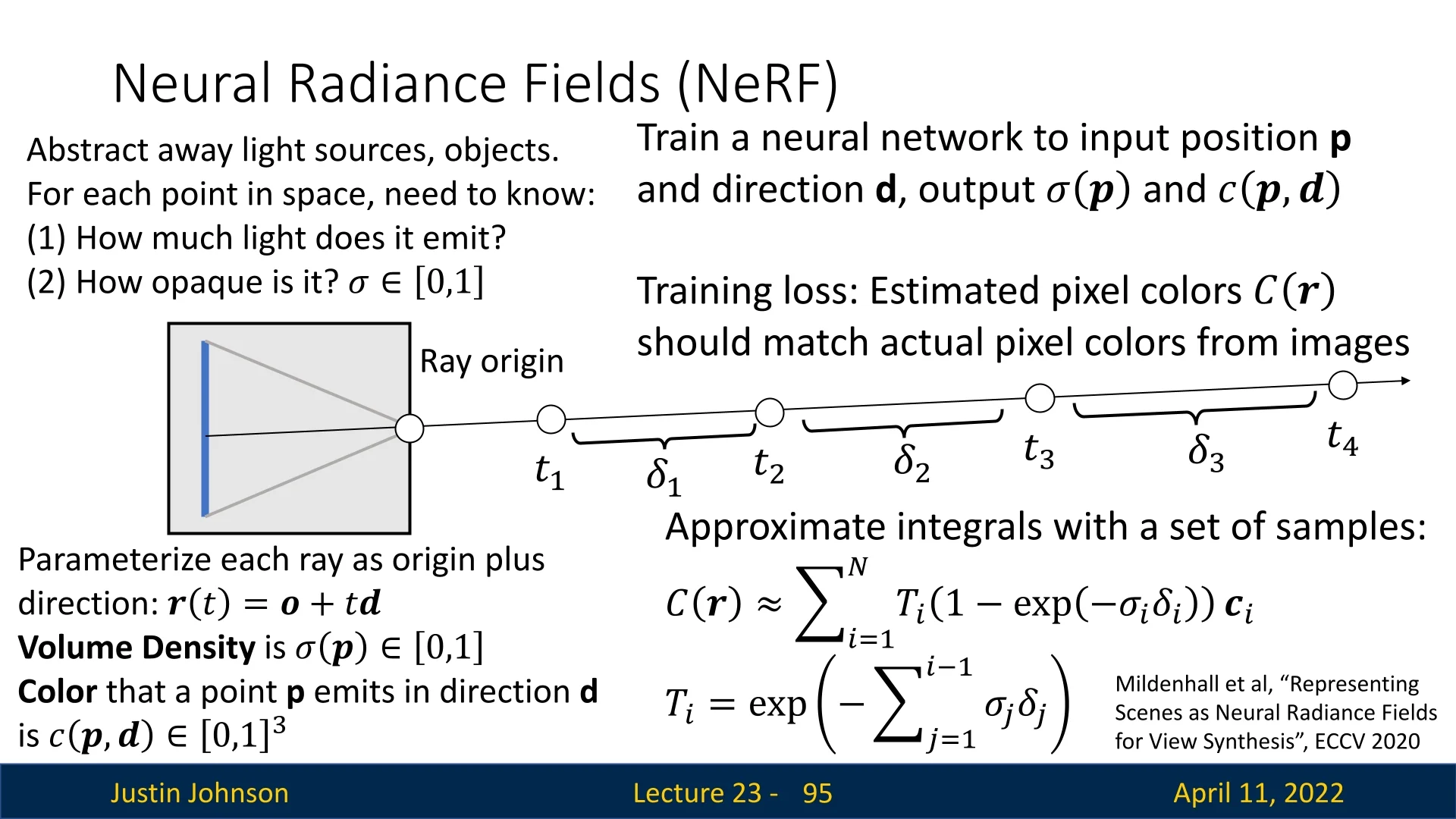
From Pixel Color to Supervised 3D Sampling Once a ray \( \mathbf {r}(t) = \mathbf {o} + t\mathbf {d} \) is constructed for pixel \( (u, v) \), NeRF must supervise the unknown 3D scene based solely on the pixel’s ground-truth color \( \mathcal {C}(\mathbf {r}) \in [0,1]^3 \). There is no direct annotation for which points along the ray contain surfaces or emit light; supervision is available only at the endpoint of the entire rendering process. The core insight of NeRF is that even this sparse signal is sufficient: if a radiance field is to match all observed views, it must explain how light accumulates along each ray to produce the correct color.
To turn this sparse supervision into dense learning signal, NeRF samples \( N \) 3D points along the ray. Although these points differ in location \( \mathbf {r}(t_i) \), they all share the same viewing direction \( \mathbf {d} \), which defines how color should vary based on perspective. Each point is passed to a neural network \( f_\theta \), yielding:
\[ \sigma _i := \sigma (\mathbf {r}(t_i)), \qquad \mathbf {c}_i := \mathbf {c}(\mathbf {r}(t_i), \mathbf {d}), \]
where \( \sigma _i \in \mathbb {R}_{\geq 0} \) is the predicted volume density and \( \mathbf {c}_i \in [0,1]^3 \) is the view-dependent color. These are combined via front-to-back alpha compositing to produce an estimated pixel color: \[ \hat {\mathcal {C}}(\mathbf {r}) = \sum _{i=1}^{N} T_i \cdot \alpha _i \cdot \mathbf {c}_i, \qquad \alpha _i = 1 - \exp (-\sigma _i \delta _i), \qquad T_i = \prod _{j=1}^{i-1} (1 - \alpha _j), \] where \( \delta _i = t_{i+1} - t_i \) is the spacing between samples.
This entire pipeline is fully differentiable. NeRF defines an \( \ell _2 \) reconstruction loss between the rendered color and ground truth: \[ \mathcal {L}_{\mbox{recon}} = \left \| \hat {\mathcal {C}}(\mathbf {r}) - \mathcal {C}(\mathbf {r}) \right \|_2^2, \] and uses backpropagation to update the MLP weights \( \theta \). Each pixel thus supervises not just a point sample, but an entire ray of 3D locations, encouraging the network to learn a coherent global representation.
Hierarchical Sampling: Coarse-to-Fine Supervision and Loss To allocate computation effectively along each ray, NeRF employs a coarse-to-fine sampling strategy using two separate but jointly trained MLPs. The first stage explores the ray with uniform coverage, while the second concentrates on promising regions—typically those with higher predicted opacity. Both networks are optimized with ground-truth pixel color supervision, allowing the model to learn geometry and appearance jointly.
- Coarse stage (exploration): NeRF begins by drawing \( N_c \) samples along the ray \( \mathbf {r}(t) = \mathbf {o} + t\mathbf {d} \) using stratified sampling. The interval \( [t_n, t_f] \) is divided into equal-width bins, and one depth value is jittered uniformly within each: \[ t_i \sim \mathcal {U}\left [ \frac {i-1}{N_c}(t_f - t_n) + t_n,\; \frac {i}{N_c}(t_f - t_n) + t_n \right ]. \] Each corresponding 3D location \( \mathbf {r}(t_i) \) is passed through the coarse MLP, which predicts density \( \sigma _i \) and radiance \( \mathbf {c}_i \). These are composited into an initial pixel color estimate \( \hat {\mathcal {C}}_{\mbox{coarse}}(\mathbf {r}) \), supervised by the known ground-truth color \( \mathcal {C}(\mathbf {r}) \) from the training image: \[ \mathcal {L}_{\mbox{coarse}} = \left \| \hat {\mathcal {C}}_{\mbox{coarse}}(\mathbf {r}) - \mathcal {C}(\mathbf {r}) \right \|_2^2. \]
- Fine stage (refinement): The coarse compositing weights \[ w_i := T_i \cdot \alpha _i \] define a piecewise PDF over the ray that emphasizes surface-adjacent regions. From this distribution, \( N_f \) additional samples \( \{ t_j' \} \) are drawn. These fine samples are merged with the coarse ones, and the union is passed to a second fine MLP, which outputs improved density and color estimates. These are composited into a higher-resolution prediction \( \hat {\mathcal {C}}_{\mbox{fine}}(\mathbf {r}) \), also supervised via a reconstruction loss: \[ \mathcal {L}_{\mbox{fine}} = \left \| \hat {\mathcal {C}}_{\mbox{fine}}(\mathbf {r}) - \mathcal {C}(\mathbf {r}) \right \|_2^2. \]
The final training objective combines both stages: \[ \mathcal {L}_{\mbox{total}} = \mathcal {L}_{\mbox{coarse}} + \mathcal {L}_{\mbox{fine}}. \]
This coarse-to-fine architecture allows the coarse MLP to guide sampling adaptively—allocating more effort where surfaces are likely to be.
Why This Works: Learning Geometry from Pixel Colors At a glance, NeRF’s approach seems almost paradoxical: the model has no knowledge of surfaces, yet learns to infer geometry purely from pixel-level color supervision. This works because each pixel’s color constrains the entire ray beneath it. By rendering sampled 3D points into a single prediction \( \hat {\mathcal {C}}(\mathbf {r}) \), NeRF creates a differentiable bridge between thousands of possible 3D explanations and a single observed RGB triplet.
- Supervision Distribution: Although we supervise only one color per ray, gradients flow through all points that contributed to the composited prediction—distributing signal to every sample \( \mathbf {r}(t_i) \).
- Emergent Surfaces: The only way to consistently satisfy these ray-level constraints across all views is to assign high density \( \sigma \) to points where many rays agree on a visual transition—i.e., surfaces.
- Efficient Focus: Hierarchical sampling ensures that fine-level computation is concentrated around informative regions, reducing noise and improving convergence.
Together, this architecture allows NeRF to transform sparse RGB supervision into a globally consistent volumetric reconstruction. It replaces dense 3D supervision with a powerful ray-based training signal that not only enables photorealism, but also implicitly discovers geometry.
A Differentiable Rendering Engine for View Synthesis The NeRF rendering pipeline is fully differentiable: all operations—depth sampling, MLP querying, and the computation of per-sample density \( \sigma _i \), color \( \mathbf {c}_i \), opacity \( \alpha _i \), transmittance \( T_i \), and accumulated pixel color—are smooth and continuous. This enables the system to be trained end-to-end via gradient descent, minimizing a reconstruction loss between predicted colors \( \hat {\mathcal {C}}(\mathbf {r}) \) and ground-truth image values \( \mathcal {C}(\mathbf {r}) \).
At inference time, this same mechanism enables photorealistic novel view synthesis: given an unseen camera pose, rays are cast through each pixel and evaluated against the learned radiance field to render new, realistic images of the scene.
To support such high-fidelity synthesis, the underlying model must capture detailed scene geometry and appearance, including fine spatial structure and subtle view-dependent effects. NeRF achieves this by modeling the radiance field as a continuous function parameterized by a compact Multi-Layer Perceptron (MLP), which maps each sampled 5D coordinate \( (\mathbf {x}, \mathbf {d}) \) to a scalar volume density \( \sigma \) and a direction-conditioned color \( \mathbf {c} \).
In practice, this modeling approach must be paired with careful input parameterization and architectural choices to ensure stable optimization and accurate reconstruction. The next subsection introduces the key components—starting with how raw input coordinates are encoded and how the radiance field network is structured to support expressive, high-quality view synthesis.
23.9.5 Practical Implementation Details
To realize photorealistic view synthesis in practice, Neural Radiance Fields (NeRF) rely on careful architectural design choices and encoding strategies that address the limitations of standard neural networks in representing fine spatial and angular detail. We begin by discussing the core technique that enables high-frequency reconstruction—positional encoding—and then present the structure of the neural network used to model the radiance field.
Positional Encoding for High-Frequency Detail
A key challenge in training Multi-Layer Perceptrons (MLPs) to represent complex 3D scenes is their inherent spectral bias—a tendency to learn and prioritize low-frequency (smooth) functions during optimization [518]. This empirically common phenomenon limits an MLP’s ability to accurately reconstruct fine geometric detail or rapidly varying texture when operating directly on raw spatial or angular coordinates.
In the context of NeRF, this bias manifests as blurry surfaces, oversmoothed edges, and a general failure to capture high-frequency content such as thin structures, sharp contours, or specular highlights. Though MLPs are universal function approximators, their convergence rate for high-frequency components is significantly slower [522]. This results in poor early representations and long training times for high-resolution detail, with the network often getting stuck in smooth approximations of the scene.
This limitation stems from the inductive properties of MLPs: small changes in the input—such as a slight shift in spatial location or viewing angle—tend to produce small changes in the output, especially when the input space is unstructured and low-dimensional. As shown in Fourier-domain analyses of coordinate-based MLPs, deeper or wider networks alone do not resolve this issue [518, 522]. High-frequency functions require precise, localized output variations, which are difficult to express using standard activation dynamics and gradient descent unless the input is carefully encoded.
To address this, NeRF introduces a simple yet powerful solution: positional encoding. Instead of feeding raw 3D coordinates \( \mathbf {x} \in \mathbb {R}^3 \) and 2D viewing directions \( \mathbf {d} \in \mathbb {S}^2 \) directly into the MLP, each scalar input value \( p \) is transformed by a fixed encoding function \( \gamma (p) \), which projects it into a high-dimensional space of sinusoids at exponentially increasing frequencies: \[ \gamma (p) = \left ( \sin (2^0 \pi p), \cos (2^0 \pi p), \ldots , \sin (2^{L-1} \pi p), \cos (2^{L-1} \pi p) \right ). \] This transformation is applied independently to each component of \( \mathbf {x} \) and \( \mathbf {d} \), resulting in a total input dimensionality of \( 3(2L + 1) + 3(2L' + 1) \) when using \( L \) frequency bands for position and \( L' \) for direction.
The motivation behind this transformation is grounded in Fourier analysis. Positional encoding effectively “injects” a spectrum of basis functions into the input space, allowing the network to represent high-frequency signals through linear combinations of these sinusoids in the first layer. Rather than forcing the MLP to learn such frequency structure through deep nonlinear compositions—which is inefficient and prone to convergence issues—this encoding enables the model to access high-frequency expressivity from the start.
Empirical results confirm the importance of this technique: models trained without positional encoding exhibit significantly reduced visual fidelity, slower convergence, and inability to recover fine detail. In contrast, networks using positional encoding successfully reconstruct sharp surfaces, reflective materials, and detailed textures [442]. Subsequent theoretical analysis shows that positional encoding modifies the neural tangent kernel (NTK) of the MLP to increase its bandwidth and flatten its spectrum, improving gradient flow and allowing more balanced learning of low- and high-frequency components [624].
Intuition Behind Positional Encoding To grasp the role of positional encoding in NeRF, it helps to consider how an MLP ”sees” space. When fed raw spatial or angular coordinates, the network operates in a smooth, low-frequency regime: small changes in input tend to produce only small changes in output. While this behavior is appropriate for modeling gradual variations, it becomes a liability when the scene contains sharp edges, fine textures, or high-frequency lighting effects. In such cases, the desired output—radiance or density—may change rapidly over very small spatial intervals. Standard MLPs struggle to express such localized variation due to their spectral bias toward smooth functions.
This limitation arises because MLPs must synthesize high-frequency behavior through deep compositions of nonlinearities, which is both inefficient and slow to converge. As a result, renderings trained on raw coordinates tend to exhibit blurred contours and oversmoothed detail—especially near thin structures or specular surfaces.
Positional encoding addresses this problem by enriching each scalar input with a fixed set of sinusoidal functions at multiple frequencies: \[ \gamma (p) = \left ( \sin (2^0 \pi p), \cos (2^0 \pi p), \ldots , \sin (2^{L-1} \pi p), \cos (2^{L-1} \pi p) \right ). \] This mapping transforms the input space such that small changes in position or direction can produce large, expressive shifts in the encoded representation—especially in the higher-frequency components. Crucially, this does not destabilize the network; rather, it gives the MLP access to a spectrum of variation that it can combine linearly in the first layer, allowing it to model both smooth regions and sharp transitions with ease.
An intuitive analogy is that of a painter. Feeding raw coordinates into an MLP is like giving an artist only broad brushes: suitable for outlining large shapes, but incapable of capturing intricate structure. Positional encoding equips the model with a complete set of tools—from coarse rollers to ultra-fine brushes—so it can render both global layout and detailed texture. The high-frequency “ink” is already embedded in the input; the MLP need only learn how to blend it.
Importantly, positional encoding does not increase the model’s depth or parameter count. Instead, it reformulates the input representation to align with the underlying complexity of the radiance field. By embedding frequency structure directly into the input space, it enables the network to express high-detail content from the very beginning of training—accelerating convergence and dramatically improving reconstruction fidelity.
Network Architecture and Functional Mapping
The NeRF network is a fully-connected MLP with ReLU activations. Its design reflects a structural separation between geometric and appearance representations, achieved via a two-stage processing pipeline.
The input 3D location \( \mathbf {x} \), encoded via \( \gamma (\mathbf {x}) \), is passed through a series of \( 8 \) layers, each with \( 256 \) units and ReLU activations. A skip connection concatenates the original positional encoding \( \gamma (\mathbf {x}) \) to the output of the 4th layer. This first stage outputs two quantities:
- A scalar volume density \( \sigma \), representing how likely the ray is to terminate at that location.
- A learned feature vector \( \mathbf {h} \in \mathbb {R}^{256} \) representing local geometry and appearance context.
To model view-dependent effects, the encoded viewing direction \( \gamma (\mathbf {d}) \) is concatenated with \( \mathbf {h} \), and passed through an additional 1-hidden-layer MLP (with 128 units) to predict RGB color \( \mathbf {c} \in [0,1]^3 \).
This separation allows the network to maintain consistent density across all directions while permitting directional variation in emitted color, enabling the modeling of non-Lambertian surfaces such as specular highlights and reflections.
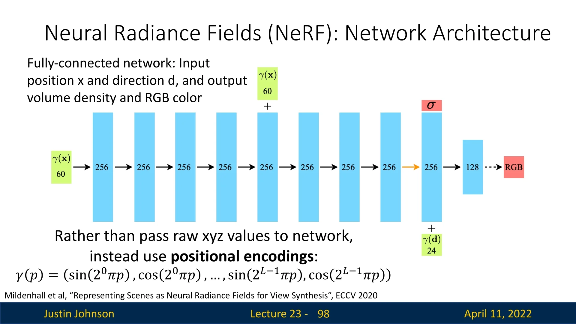
Together, the positional encoding and network design allow NeRF to map input rays to realistic colors with high accuracy.
Training vs. Inference: Pixel-Level Supervision and Scene Reconstruction
Although NeRF is trained using a loss defined at the level of individual image pixels, its learned representation is fundamentally volumetric: a continuous 5D field that maps 3D spatial locations and 2D viewing directions to color and density. A natural question arises—how can independent pixelwise comparisons to ground-truth RGB values yield a globally consistent 3D scene representation?
The key insight is that each pixel, while evaluated in isolation during training, arises from a unique ray that passes through the shared 3D environment. As the model is optimized to match the color seen along each ray, it must learn a radiance field whose volumetric structure explains not just isolated pixels but the appearance of entire scenes across multiple views. If the model were to hallucinate geometry or color in one ray that contradicts observations in another, the accumulated error across views would remain high. Thus, consistency across views serves as a powerful regularizer: even though supervision is pixel-local, the shared volumetric MLP must reconcile all views into a coherent underlying scene.
Training Procedure NeRF is trained on a dataset of posed RGB images \( \{ I_k \}_{k=1}^K \), where each image \( I_k \) is accompanied by known camera intrinsics and extrinsics. For each scene, a dedicated neural radiance field is trained from scratch using all available views—unlike models trained across multiple scenes, NeRF does not require train/validation/test image splits for learning. Instead, novel view synthesis is evaluated on held-out camera poses after scene reconstruction is complete.
At each iteration, a batch of camera rays \( \mathbf {r} = \mathbf {o} + t\mathbf {d} \) is randomly sampled from the set of all training pixels across all images. Each ray is then evaluated using a two-stage hierarchical sampling scheme. In the first pass, \( N_c \) coarse depth samples \( \{ t_i \} \) are drawn along the ray via stratified sampling, and the corresponding 3D points \( \mathbf {r}(t_i) \) are passed through the MLP to predict volume densities \( \sigma _i \) and view-dependent colors \( \mathbf {c}_i \). The coarse rendering \( \hat {\mathcal {C}}_c(\mathbf {r}) \) is computed using discrete volume rendering.
These weights are then used to inform a second round of importance sampling, focusing on regions of high density. An additional \( N_f \) fine samples are drawn along each ray and passed through a separate MLP (or the same MLP reused) to produce the final rendering \( \hat {\mathcal {C}}_f(\mathbf {r}) \). Both renderings are supervised against the ground-truth pixel color \( \mathcal {C}(\mathbf {r}) \) using an \(\ell _2\) loss: \[ \mathcal {L}_{\mbox{train}} = \sum _{\mathbf {r} \in \mathcal {B}} \left [ \left \| \hat {\mathcal {C}}_c(\mathbf {r}) - \mathcal {C}(\mathbf {r}) \right \|_2^2 + \left \| \hat {\mathcal {C}}_f(\mathbf {r}) - \mathcal {C}(\mathbf {r}) \right \|_2^2 \right ], \] where \( \mathcal {B} \) is the minibatch of rays. This loss is minimized via gradient descent, with gradients backpropagated through the entire rendering pipeline—including MLP evaluations, opacity computation, and alpha compositing. Over time, this process encourages the network to discover a coherent 3D radiance field that explains all views simultaneously.
Although the training signal is defined at the pixel level, the MLP must synthesize a global function that satisfies all camera rays across the scene.
Inference Procedure At inference time, NeRF renders novel views from previously unseen camera poses. Given new camera intrinsics and extrinsics—either provided as ground truth or estimated via structure-from-motion tools like COLMAP—a ray is cast through the center of each pixel in the desired output image resolution. For each ray \( \mathbf {r}(t) = \mathbf {o} + t\mathbf {d} \), NeRF applies the same stratified and hierarchical sampling strategy used during training.
Sampled 3D points along the ray are passed through the trained MLP to predict volume densities \( \sigma _i \) and view-dependent colors \( \mathbf {c}_i \). These are combined via discrete volume rendering: \[ \hat {\mathcal {C}}(\mathbf {r}) = \sum _{i=1}^{N} T_i \cdot \alpha _i \cdot \mathbf {c}_i, \] where \( \alpha _i \) and \( T_i \) represent the segment opacity and transmittance, respectively. This process is repeated independently for every ray—effectively synthesizing the image pixel by pixel using only forward passes through the network.
Inference is parallelizable across rays and pixels, making it well-suited for GPU execution. However, it remains computationally intensive: each output frame requires evaluating hundreds of MLP queries per pixel. This results in high-fidelity but slow rendering, with original NeRF models taking tens of seconds per image on modern GPUs for small scenes up to days for more complex and high-resolution one on weaker GPUs.
Why Pixel-Level Supervision Works Although NeRF is trained with per-pixel supervision, it does not learn isolated 2D mappings for each image. Instead, the volumetric rendering process couples every pixel to a ray that traverses the 3D scene, and these rays intersect and overlap across views. As a result, the color of each pixel depends on the shared radiance field that defines density and appearance throughout space.
This coupling turns local pixel errors into global constraints: an incorrect prediction at any point along a ray affects not just one pixel, but all others whose rays pass through the same region. Minimizing the total photometric loss across all training images therefore requires the model to discover a single, consistent radiance field that simultaneously explains all views. In this sense, NeRF performs multi-view 3D reconstruction not through explicit geometry, but through radiance field alignment guided by view-dependent color integration.
The shared MLP must assign densities and colors that are jointly plausible across viewpoints—encoding accurate 3D structure, coherent surface geometry, and realistic appearance effects such as specularities or occlusions. Crucially, this global consistency acts as an implicit regularizer: if a sharp edge or fine surface detail is modeled inconsistently across views, the resulting rendering error remains high and drives the network to correct it. This prevents the network from overfitting to individual images and enforces smooth, physically plausible reconstructions.
Outlook The training and inference procedures outlined above empower NeRF to produce photorealistic images from novel viewpoints, relying on learned volumetric representations encoded within a neural network. However, this expressivity comes at a significant computational cost: each frame requires casting thousands of rays and performing hundreds of MLP evaluations per pixel, both during optimization and at test time. In the parts that follow, we examine NeRF’s empirical performance through experiments and ablations, before turning to its limitations and the growing body of work aimed at improving efficiency, scalability, and generalization.
23.9.6 Experiments and Ablation Studies
To validate the NeRF architecture, Mildenhall et al. [442] conducted extensive experiments on both synthetic and real-world datasets. These included comparisons with prior methods and ablation studies to isolate the contributions of key design components.
Quantitative and Qualitative Evaluation
To assess the effectiveness of NeRF, Mildenhall et al. [442] evaluated their model on two distinct datasets:
- Realistic Synthetic 360\(^\circ \): A custom Blender-rendered dataset of eight scenes, each containing complex geometry and non-Lambertian materials. Each scene provides 100 training views and 200 held-out test views at a resolution of \(800 \times 800\) pixels.
- Real Forward-Facing: A real-world dataset derived from handheld captures of eight indoor/outdoor scenes. These images were processed with COLMAP to extract camera poses, and 1/8 of the views were held out for evaluation.
Evaluation used the following standard image quality metrics:
- PSNR (Peak Signal-to-Noise Ratio): A log-domain pixel-wise fidelity metric, expressed in decibels. Higher values indicate better reconstruction accuracy.
- SSIM (Structural Similarity Index Measure): A perceptual metric capturing local luminance, contrast, and structure similarity. Ranges from 0 to 1; higher is better.
- LPIPS (Learned Perceptual Image Patch Similarity): Measures perceptual similarity using deep features. Lower values indicate better perceptual fidelity.
These results highlight NeRF’s significant improvement over prior methods. Compared to SRN and LLFF, NeRF improves PSNR by more than 6 dB, increases structural similarity, and cuts LPIPS perceptual error nearly in half.
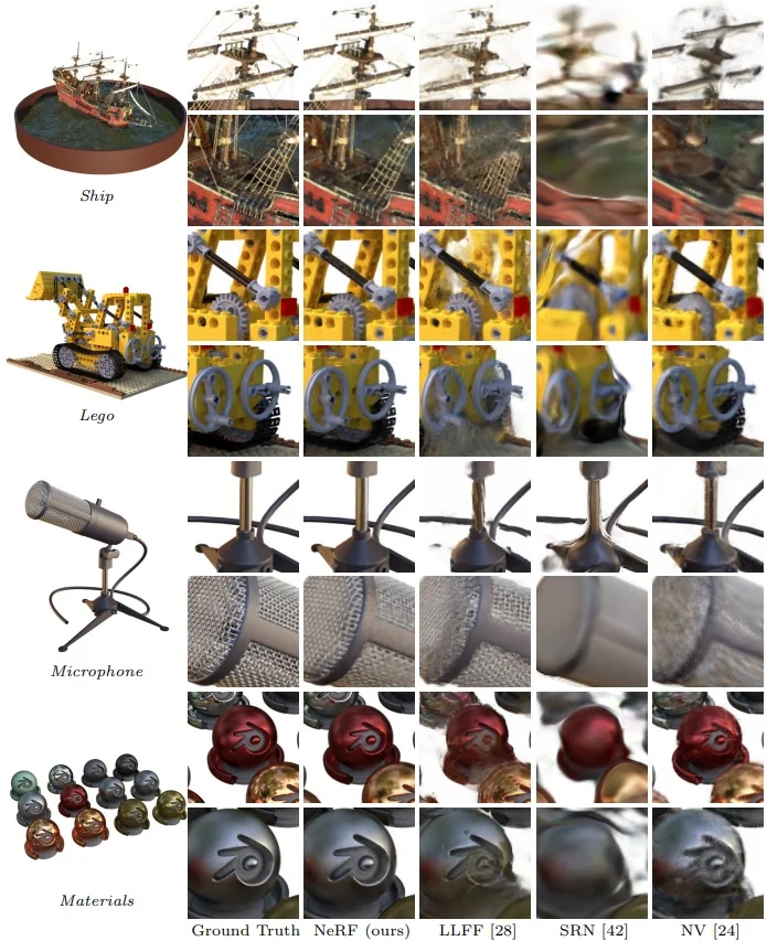
Ablation Studies
To understand which components most influence NeRF’s performance, the authors conducted a series of ablations on the Realistic Synthetic 360° dataset. The study evaluated the effects of disabling positional encoding (PE), view-dependence (VD), and hierarchical sampling (H), as well as reducing the number of input views and adjusting frequency hyperparameters.
| Row | Configuration | \(L\) | #Img | \((N_c, N_f)\) | PSNR |
|---|---|---|---|---|---|
| 1 | No PE, VD, H | – | 100 | (256, –) | 26.67 |
| 2 | No Positional Encoding | - | 100 | (64, 128) | 28.77 |
| 3 | No View Dependence | 10 | 100 | (64, 128) | 27.66 |
| 4 | No Hierarchical Sampling | 10 | 100 | (256, –) | 30.06 |
| 5 | Far fewer images | 10 | 25 | (64, 128) | 27.78 |
| 6 | Fewer images | 10 | 50 | (64, 128) | 29.79 |
| 7 | Lower frequency (\(L=5\)) | 5 | 100 | (64, 128) | 30.59 |
| 8 | Higher frequency (\(L=15\)) | 15 | 100 | (64, 128) | 30.81 |
| 9 | Full Model (baseline) | 10 | 100 | (64, 128) | 31.01 |
Key observations:
- Positional Encoding (PE) is indispensable for capturing high-frequency details such as edges, textures, and specular boundaries. Disabling PE (Row 2) reduces PSNR from 31.01 to 28.77, a 2.24 dB drop. This confirms that raw 3D inputs (xyz) are insufficient due to the spectral bias of MLPs, which favor learning smooth, low-frequency functions. PE provides the network with high-frequency sine and cosine basis functions, significantly improving representation capacity.
- View Dependence (VD) enables NeRF to model view-dependent effects like specular highlights and non-Lambertian reflectance. Removing view direction inputs (Row 3) yields a PSNR of 27.66, a 3.35 dB drop from the full model. Visually, surfaces appear matte and unrealistically static across viewpoints. This component is essential for photorealism and dynamic lighting effects.
- Hierarchical Sampling (H) improves both accuracy and training efficiency by allocating more samples to high-opacity regions. Disabling it (Row 4) leads to a moderate drop of 0.95 dB (PSNR 30.06 vs. 31.01) and increases training cost. While the rendering quality remains competitive, the uniform sampling strategy is computationally inefficient, often allocating samples to empty space, causing more noisy predictions.
- Number of Input Views directly affects reconstruction quality. Reducing the number of input images from 100 (Row 9) to 50 (Row 6) or 25 (Row 5) lowers PSNR to 29.79 and 27.78, respectively. Notably, even with only 25 views, NeRF still outperforms all prior baselines evaluated on 100 views, demonstrating robustness. However, performance declines in occluded or textureless regions, especially under extreme sparsity.
- Frequency Parameter \( L \) controls the number of sine/cosine frequency bands in PE. Lowering \( L \) to 5 (Row 7) leads to underfitting, decreasing PSNR to 30.59. Increasing \( L \) to 15 (Row 8) slightly reduces performance (30.81), likely due to overfitting or gradient instability. Thus, \( L = 10 \) (Row 9) offers a well-balanced tradeoff between expressivity and stability.
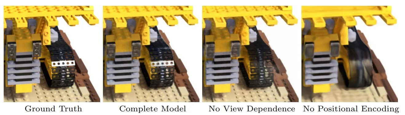
These experiments validate the necessity of all three architectural innovations—Fourier-based input encoding, view-dependent radiance modeling, and hierarchical sampling—for achieving NeRF’s high-fidelity results. Removing any one of these leads to degraded reconstructions and/or reduced realism, and sometimes even to slower convergence.
23.9.7 Limitations of the Original NeRF Architecture
Despite the seminal impact of NeRF on 3D view synthesis, the original architecture introduced by [442] exhibits several foundational limitations that have since motivated a wave of follow-up research. These limitations are not isolated flaws but rather systemic consequences of NeRF’s core design—a monolithic, scene-specific MLP that implicitly encodes geometry and radiance in millions of uninterpretable parameters. This subsection outlines six key bottlenecks, each of which inspired entire subfields of NeRF variants and accelerations.
1. Computational Inefficiency: Prohibitive Training and Inference Time
The most immediate drawback of NeRF is its extreme computational cost. Training a single scene typically requires tens to hundreds of GPU-hours, rendering it impractical for real-time or interactive use. Even inference is slow: to render a single image, NeRF must trace thousands of rays and query the MLP hundreds of times per ray, leading to total long runtimes per frame. This high latency renders applications such as virtual walkthroughs, VR/AR environments, or online editing infeasible without significant acceleration strategies. As we will see in subsequent parts, this limitation motivated a wave of speed-focused methods including Plenoxels [162], Instant-NGP [457], and TensoRF [80].
2. Data Hungriness and Pose Sensitivity
NeRF requires dense and accurate supervision: typically 100 or more posed input images for each scene. With sparse views, the model tends to overfit, memorizing training pixels and producing incorrect geometry with “floaters”—hallucinated density blobs in empty space. Moreover, NeRF assumes externally provided camera poses, often estimated via SfM pipelines such as COLMAP. Pose errors—especially in large or low-texture scenes—can severely degrade reconstruction quality, introducing ghosting and multi-exposure artifacts. These dependencies make NeRF fragile in real-world settings, where pose estimation and dense capture are often unavailable or noisy.
3. Static Scene Assumption
The original NeRF architecture assumes the scene is completely static during capture. Even minor motion—e.g., waving trees, moving pedestrians, changing shadows—violates this assumption. Since the MLP must learn a consistent radiance field, it fails to reconcile inconsistencies in dynamic scenes, leading to ghosting, blur, or averaged-out artifacts. Consequently, NeRF cannot model temporal phenomena or non-rigid deformation without significant modification. This limitation gave rise to dynamic variants such as D-NeRF [502] and subsequent temporally aware architectures.
4. Poor Scalability to Large or Unbounded Scenes
The architectural choice to encode an entire scene in a single MLP imposes a severe scalability bottleneck. As the physical extent of the scene increases—e.g., modeling a building, city block, or 360° landscape—the network’s finite capacity becomes insufficient. The result is coarse geometry and low-frequency, blurry reconstructions. Additionally, the fixed near and far depth bounds used in NeRF’s ray sampling mechanism are ill-suited for outdoor, forward-facing, or horizon-spanning scenes. These challenges spurred modular representations such as Block-NeRF [623], which decompose large scenes into a grid of smaller NeRFs with overlapping coverage and shared appearance embeddings.
5. Inadequate Robustness to Real-World Imaging Conditions
Most NeRF experiments are performed on sanitized datasets of clean, low dynamic range (LDR), well-lit images. In contrast, real-world imagery often suffers from HDR saturation, sensor noise, motion blur, lens artifacts, and non-uniform exposure. The original NeRF, trained on LDR values, fails to reconstruct true radiance under such conditions. Moreover, it lacks mechanisms for denoising or compensating for exposure variation. Recent works like RawNeRF [443] address this by operating on raw sensor data directly, enabling robust HDR synthesis and improved fidelity under challenging lighting.
6. Non-Editable and Opaque Representation
Finally, NeRF’s learned radiance field is entirely implicit—stored in millions of weights of an MLP. This makes downstream operations such as object editing, segmentation, relighting, or geometry manipulation extremely difficult. In traditional 3D representations (e.g., meshes or voxels), editing corresponds to direct manipulation of structures with semantic meaning. In NeRF, by contrast, even deleting an object or changing its appearance would require retraining the model or resorting to finetuning tricks. This “black-box” nature remains a key challenge and an active area of research. Later approaches like Control-NeRF [325] and NeRFShop [271] aim to bridge this gap by decoupling editable features from rendering logic.
Summary The limitations of the original NeRF—its slowness, data hungriness, fragility, and lack of editability—are all downstream consequences of its monolithic, implicit MLP-based design. Recognizing this, researchers have shifted towards more modular, explicit, and hybrid representations. As we will see in upcoming parts, these improvements not only alleviate NeRF’s bottlenecks but also expand its capabilities to dynamic scenes, outdoor environments, real-time applications, and creative workflows.
Enrichment 23.10: NeRF: Acceleration and Representation Revisions
While the original NeRF architecture achieved groundbreaking results in novel view synthesis, it suffered from severe computational bottlenecks and restrictive design choices. This limitation gave rise to two key research directions:
- Making NeRFs faster: by improving both scene representation and the rendering pipeline;
- Rethinking representation itself: by exploring whether implicit MLPs are the optimal abstraction for radiance fields.
This subsection surveys the most prominent families of acceleration techniques and scene representation variants—each representing a distinct research trajectory in the evolving landscape of neural rendering.
Explicit Voxel and Point Grid Representations A fundamental insight that motivated the first wave of NeRF accelerations is that the full power of an MLP may not be necessary to represent a static radiance field. In the original NeRF, each query along a ray—at a specific 3D point and viewing direction—requires a forward pass through a deep, overparameterized network. This becomes prohibitively slow when hundreds of queries must be processed per pixel in the image. If instead one could cache the radiance field explicitly in space, the model could avoid MLP evaluation altogether and retrieve color and density via simple, differentiable lookups.
This leads to a powerful tradeoff: speed versus memory. By storing radiance and density in spatial grids—either dense or sparsely populated—methods can dramatically reduce inference time and enable real-time rendering. The price is cubic memory growth with resolution, requiring careful grid design or pruning to scale. The following two methods exemplify this family of approaches.
Enrichment 23.10.1: Plenoxels: Sparse Voxel Grids with Spherical Harmonics
Plenoxels [162] introduce a fully explicit scene representation that removes neural networks from the NeRF rendering pipeline. Instead of approximating the radiance field using a continuous MLP \( f_\theta (\mathbf {x}, \mathbf {d}) \), Plenoxels define a sparse 3D voxel grid in which each voxel corner—corresponding to a 3D coordinate in space—stores:
- A scalar volume density \( \sigma \in \mathbb {R}_+ \), analogous to NeRF, encoding how much matter is present at that spatial location.
- Spherical harmonics (SH) coefficients for view-dependent RGB color. For SH degree \( l \), each corner stores \( (l + 1)^2 \) coefficients per color channel (e.g., \( 9 \) per channel for \( l = 2 \)): \[ \mathbf {c}(\mathbf {x}, \mathbf {d}) = \sum _{\ell =0}^{l} \sum _{m=-\ell }^{\ell } \mathbf {a}_{\ell m} \cdot Y_{\ell m}(\mathbf {d}), \] where \( Y_{\ell m}(\mathbf {d}) \) is the SH basis evaluated at viewing direction \( \mathbf {d} \), and \( \mathbf {a}_{\ell m} \in \mathbb {R}^3 \) are the learnable RGB coefficients.
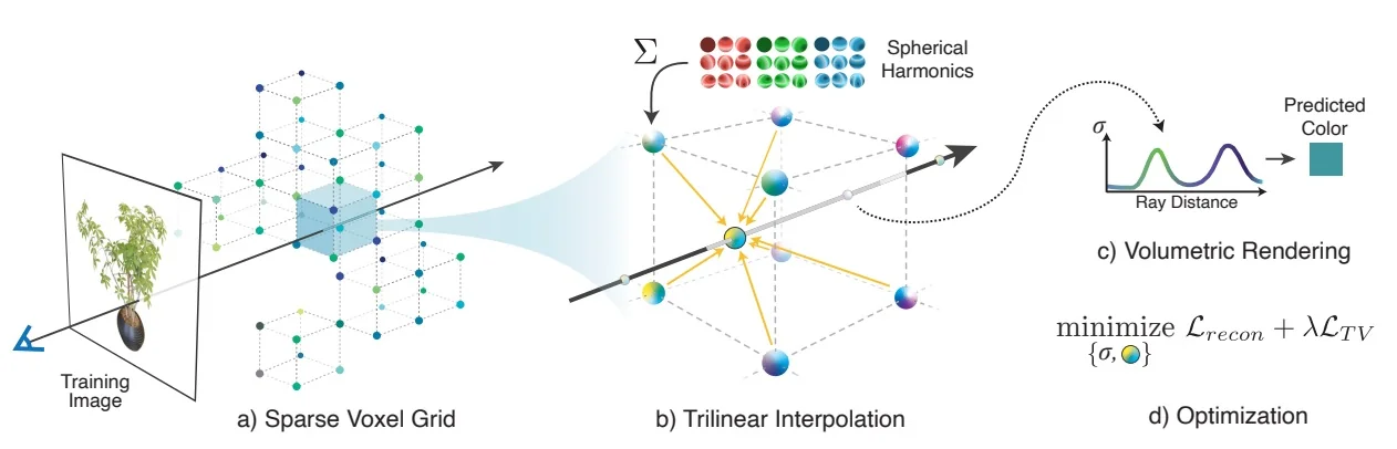
Inference and Volume Rendering. For each ray \( \mathbf {r}(t) = \mathbf {o} + t\mathbf {d} \), Plenoxels sample a set of points \( \mathbf {r}(t_i) \) within the interval \( [t_n, t_f] \), as in NeRF. For each point:
- The trilinear interpolation of densities and SH coefficients is computed from the eight corners of the voxel enclosing \( \mathbf {r}(t_i) \).
- The interpolated SH coefficients are combined with the viewing direction \( \mathbf {d} \) via SH basis functions to compute the radiance \( \mathbf {c}_i \in [0,1]^3 \).
- These values \( (\sigma _i, \mathbf {c}_i) \) are integrated along the ray using the same differentiable alpha compositing rule as NeRF: \[ \hat {\mathcal {C}}(\mathbf {r}) = \sum _{i=1}^N T_i \cdot \alpha _i \cdot \mathbf {c}_i, \quad \alpha _i = 1 - \exp (-\sigma _i \delta _i), \quad T_i = \prod _{j=1}^{i-1}(1 - \alpha _j). \]
This process is far more efficient than evaluating an MLP for each query point.
Training via Reconstruction Loss. Plenoxels are trained using the same loss as NeRF. For a ray with known ground-truth color \( \mathcal {C}(\mathbf {r}) \), the predicted color \( \hat {\mathcal {C}}(\mathbf {r}) \) is supervised by: \[ \mathcal {L}_{\mbox{recon}} = \left \| \hat {\mathcal {C}}(\mathbf {r}) - \mathcal {C}(\mathbf {r}) \right \|_2^2. \] To ensure smoothness and avoid artifacts, the authors also apply a total variation regularization term to both the SH coefficients and densities.
Why Spherical Harmonics? Spherical harmonics are a compact, differentiable basis for modeling smooth directional variation. At each spatial point, SHs allow the color to change with viewpoint (e.g., capturing specularities), while still being efficient to store and evaluate. Importantly, their basis functions \( Y_{\ell m}(\mathbf {d}) \) are fixed and directional—so the only learnable parameters are the SH coefficients per corner.
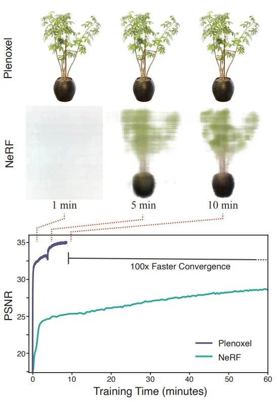
Fast Convergence via Coarse-to-Fine Refinement. The voxel grid is initialized at a low resolution (e.g., \( 128^3 \)), with voxels that have low opacity pruned early. As training progresses, high-opacity regions (likely to contain object surfaces) are adaptively subdivided into finer voxels. This hierarchical approach allows Plenoxels to focus memory and resolution only where detail is required.
Core Insight and Tradeoffs. Plenoxels’ design replaces learned neural scene functions with a sparse, explicit grid of radiance information. The grid is fully differentiable, fast to query, and optimized directly—avoiding the need for costly MLP forward passes. However, this performance comes at the cost of memory: voxel-based representations scale cubically with resolution, and require pruning and sparsity to remain tractable.
Key insight: By combining spherical harmonics with sparse voxel grids, Plenoxels offer a radiance field representation that is fast to optimize and evaluate, enabling high-quality novel view synthesis in minutes rather than hours.
Enrichment 23.10.2: DVGO: Direct Optimization on Dense Voxel Grids
Direct Voxel Grid Optimization (DVGO) [613] accelerates novel view synthesis by replacing NeRF’s implicit MLP with a fully explicit scene representation: a dense voxel grid storing volume densities and appearance features. This design allows DVGO to train up to two orders of magnitude faster than NeRF while retaining differentiable volumetric rendering.
A dense grid refers to a regular axis-aligned 3D array covering a bounded scene volume, where every voxel is allocated and updated during training—unlike sparse grids, which store only occupied regions. This simplifies memory layout and interpolation, but requires careful bounding and coarse-to-fine scheduling to manage memory usage.
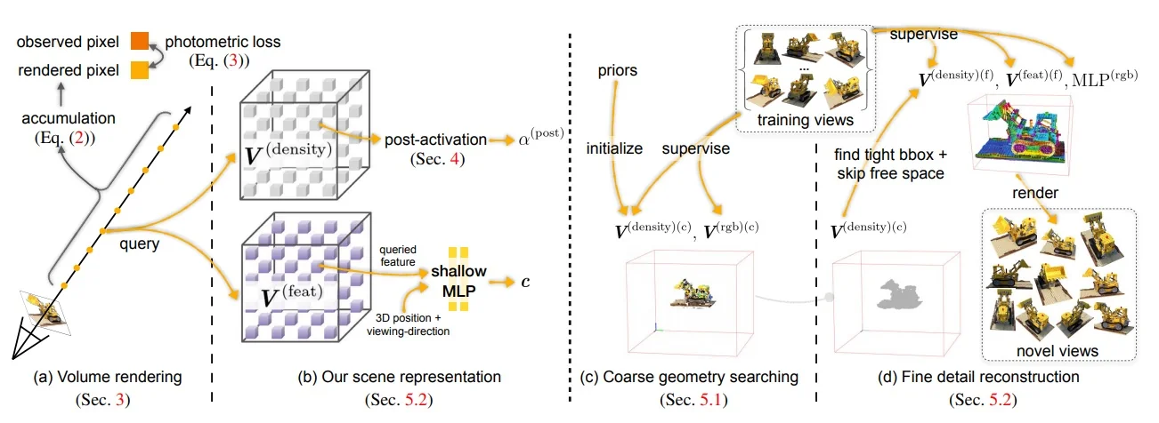
Rendering Pipeline DVGO preserves the volumetric rendering framework of NeRF but replaces the implicit MLP with an explicit, grid-based representation. The rendering process is composed of the following steps:
- 1. Ray Sampling: For each pixel, a ray is cast as \( \mathbf {r}(t) = \mathbf {o} + t\mathbf {d} \), where \( \mathbf {o} \) is the camera origin and \( \mathbf {d} \) is the viewing direction. The ray is sampled at depths \( \{t_i\}_{i=1}^N \), yielding 3D sample points \( \mathbf {x}_i = \mathbf {r}(t_i) \).
- 2. Grid Query via Trilinear Interpolation: Each point \( \mathbf {x}_i \) is mapped into the dense voxel grid. DVGO retrieves the interpolated density \( \sigma (\mathbf {x}_i) \in \mathbb {R} \) and a learned appearance feature \( \mathbf {f}(\mathbf {x}_i) \in \mathbb {R}^C \) using trilinear interpolation from the eight surrounding voxels.
-
3. Color Decoding: To produce RGB color, DVGO offers two options:
- Direct RGB: The feature \( \mathbf {f} \) is directly interpreted as an RGB vector—this is the fastest and view-independent mode.
- Tiny MLP: A shallow two-layer MLP with the viewing direction \( \mathbf {d} \) as input decodes the color as \( \mathbf {c}_i = \mbox{MLP}(\mathbf {f}, \mathbf {d}) \). This captures simple view-dependent effects at minimal cost.
- 4. Volume Rendering: Colors \( \mathbf {c}_i \) and opacities \( \alpha _i = 1 - \exp (-\sigma _i \delta _i) \) are combined using alpha compositing: \[ T_i = \prod _{j=1}^{i-1} (1 - \alpha _j), \quad \hat {\mathcal {C}}(\mathbf {r}) = \sum _{i=1}^{N} T_i \cdot \alpha _i \cdot \mathbf {c}_i. \] The model is trained to minimize the reconstruction loss: \[ \mathcal {L} = \left \| \hat {\mathcal {C}}(\mathbf {r}) - \mathcal {C}(\mathbf {r}) \right \|_2^2. \]
Coarse-to-Fine Upsampling and Fine Detail Reconstruction DVGO’s training proceeds in a progressive manner: it begins with a coarse voxel grid (e.g., \( 128^3 \)) and upsamples it at fixed iteration checkpoints (e.g., after 2k and 4k steps) to finer resolutions (e.g., \( 256^3 \), \( 512^3 \)). Each upsampling operation uses trilinear interpolation to initialize the finer grid from the coarser one. Crucially, nonlinear activations (e.g., ReLU or softplus) are applied after interpolation—this post-activation strategy enhances sharp surface modeling and reduces high-resolution artifacts.
This multi-resolution training schedule enables the model to:
- Quickly capture global geometry with minimal compute at low resolution,
- Preserve continuity and prior learning when upsampling,
- Refine high-frequency details and textures in later training phases without restarting optimization.
During inference, only the final high-resolution grid is used.
Foreground–Background Decomposition To support both bounded and unbounded scenes, DVGO introduces a two-grid decomposition. The foreground region is represented with a dense voxel grid aligned to a tight bounding box. For unbounded backgrounds (e.g., skies or distant terrain), DVGO uses a secondary cylindrical grid in log-depth space. Rays first accumulate color and opacity from the foreground; if the transmittance remains nonzero, they continue into the background grid.
DVGOv2 Improvements DVGOv2 [613] builds on DVGO with several technical enhancements that improve both training efficiency and rendering fidelity:
- Distortion-Aware Loss: A fast implementation of the distortion regularization from mip-NeRF 360 [28], reducing complexity from \( \mathcal {O}(N^2) \) to \( \mathcal {O}(N) \).
- Adaptive Learning Rate: Voxels observed from fewer views are assigned lower learning rates to reduce overfitting to sparse observations.
- Low-Opacity Initialization: The density grid is initialized to near-zero opacity to avoid redundant clouds in empty regions.
- Cuboid Grid Parameterization: Supports unbounded scenes via a contracted cuboid grid inspired by mip-NeRF 360.
These changes lead to faster convergence, better generalization, and improved visual quality, especially in complex or forward-facing scenes.
Comparison to Plenoxels and NeRF
- NeRF: Relies on a deep MLP to model density and color, requiring multiple hours of training per scene. DVGO eliminates the MLP for geometry and uses only a shallow decoder for color, yielding up to \( 100\times \) faster training.
- Plenoxels: Employs sparse voxel grids with spherical harmonics (SH) for view-dependent color. While more memory-efficient, SH can introduce ringing artifacts and requires custom CUDA kernels. DVGO, in contrast, uses dense grids and is implemented in pure PyTorch, making it easier to adopt and extend.
Efficiency and Tradeoffs Quantitative benchmarks on the LLFF dataset highlight the tradeoffs:
- Training Time: DVGOv2 converges in ˜10.9 minutes vs. 24.2 minutes for Plenoxels.
- Quality: DVGOv2 achieves slightly better PSNR (26.34 vs. 26.29) and lower LPIPS (0.197 vs. 0.210).
- Inference Time: DVGOv2 is slightly slower (0.07–0.36 s per image) than Plenoxels (˜0.0667 s), due to its dense grid.
DVGO is ideal for rapid prototyping, differentiable pipelines, and simpler research codebases. Plenoxels remains competitive in memory-constrained or real-time settings. The choice depends on application constraints: DVGO favors training speed and modularity; Plenoxels favors compactness and high-speed inference.
Performance Across Scene Types DVGO and its improved variant DVGOv2 [614] deliver strong rendering quality across diverse benchmarks while significantly accelerating training. DVGOv2 incorporates distortion-aware loss, low-opacity initialization, and adaptive learning rates for enhanced convergence, especially in real-world or unbounded settings.
| Method | Train Time | PSNR↑ | SSIM↑ | LPIPS↓ |
|---|---|---|---|---|
Synthetic-NeRF (8 scenes) |
||||
| DVGO | 14.2m | 31.95 | 0.957 | 0.053 |
| Plenoxels | 11.1m | 31.71 | 0.958 | 0.049 |
| Instant-NGP | 5.0m | 33.18 | – | – |
| TensoRF (L) | 17.6m | 33.14 | 0.963 | 0.047 |
| DVGOv2 (L) | 6.8m | 32.76 | 0.962 | 0.046 |
| Method | Train Time | PSNR↑ | SSIM↑ | LPIPS↓ |
|---|---|---|---|---|
LLFF (forward-facing) |
||||
| NeRF [442] | ˜1440m | 26.50 | 0.811 | 0.250 |
| Plenoxels | 24.2m | 26.29 | 0.839 | 0.210 |
| TensoRF (S) | 19.7m | 26.51 | 0.832 | 0.217 |
| TensoRF (L) | 25.7m | 26.73 | 0.839 | 0.204 |
| DVGOv2 w/o \(\mathcal {L}_{\mbox{dist}}\) | 13.9m | 26.24 | 0.833 | 0.204 |
| DVGOv2 | 10.9m | 26.34 | 0.838 | 0.197 |
| Method | Train Time | PSNR↑ | SSIM↑ | LPIPS↓ |
|---|---|---|---|---|
mip-NeRF 360 (unbounded) |
||||
| NeRF | hours | 24.85 | 0.659 | 0.426 |
| NeRF++ | hours | 26.21 | 0.729 | 0.348 |
| mip-NeRF 360 | hours | 28.94 | 0.837 | 0.208 |
| DVGOv2 w/o \(\mathcal {L}_{\mbox{dist}}\) | 16.4m | 24.73 | 0.663 | 0.465 |
| DVGOv2 (\(p=2\)) | 13.2m | 24.80 | 0.659 | 0.468 |
| DVGOv2 (\(p=\infty \)) | 14.0m | 25.24 | 0.680 | 0.446 |
| DVGOv2 (\(p=\infty \))* | 15.6m | 25.42 | 0.695 | 0.429 |
Final Remarks DVGO and DVGOv2 establish voxel-based grids as powerful alternatives to neural radiance fields. By combining dense 3D grids, post-activation interpolation, and shallow decoders, they offer rapid convergence with minimal architectural complexity. DVGOv2 further enhances training stability and scalability for real-world and unbounded scenes—making it a highly competitive baseline for fast and differentiable view synthesis.
Hash-Based Feature Grid Representations While voxel-based methods accelerate NeRF by caching scene representations in spatial grids, they suffer from cubic memory growth as resolution increases. To overcome this bottleneck, a new family of approaches—starting with Instant-NGP—replaces dense voxel grids with compact multiresolution hash encodings. These techniques map 3D points to feature vectors via hash tables that sparsely index multiscale grids. The result is a flexible and memory-efficient representation that supports fast training, real-time rendering, and high fidelity.
Core Tradeoff. Hash-based grids strike a balance between speed and quality, avoiding the memory overhead of dense voxel fields while adapting to scene complexity. However, they introduce stochasticity due to hash collisions—multiple spatial locations may share a feature if they fall into the same hash bucket—potentially adding noise to reconstructions. Despite this, hash encodings have proven remarkably robust and scalable across datasets.
Enrichment 23.10.3: Instant-NGP: Multiscale Hash Encoding for Real-Time NeRF
Instant-NGP [457] revolutionized radiance field rendering by achieving real-time training and inference through a novel multi-resolution hash encoding and a fully optimized GPU pipeline. The method decouples scene resolution from memory usage by mapping 3D positions to compact, trainable feature vectors via hash tables. These features, concatenated across multiple spatial scales, are passed to a small neural decoder to predict density and color.
Multiscale Hash Encoding Instant-NGP replaces dense voxel grids with a compact, adaptive alternative: a multiresolution hash grid encoding. The key idea is to approximate the benefits of a high-resolution voxel grid without paying its cubic memory cost. Instead of explicitly allocating every voxel, the method uses a hierarchy of virtual grids combined with spatial hashing and trilinear interpolation to extract meaningful features at arbitrary 3D positions.
At each level \( \ell \in \{1, \dots , L\} \), the scene is conceptually divided into a \( 2^\ell \times 2^\ell \times 2^\ell \) regular grid. For a given point \( \mathbf {x} \in \mathbb {R}^3 \), Instant-NGP performs the following steps at level \( \ell \):
- 1.
- Voxel identification: Scale \( \mathbf {x} \) to the grid resolution and identify the indices of the 8 surrounding voxel corners.
- 2.
- Hash lookup: Each corner index is passed through a fixed spatial hash function: \[ h(x, y, z) = ((x \cdot p_1) \oplus (y \cdot p_2) \oplus (z \cdot p_3)) \boldsymbolod T, \] where \( p_1, p_2, p_3 \) are large primes, \( \oplus \) denotes bitwise XOR, and \( T \) is the fixed hash table size.
- 3.
- Feature interpolation: Each hash index retrieves a trainable feature vector from a table specific to level \( \ell \). These 8 vectors are then interpolated using trilinear interpolation, weighted by the relative position of \( \mathbf {x} \) within the voxel, to obtain a level-specific embedding \( \mathbf {f}_\ell (\mathbf {x}) \in \mathbb {R}^F \).
This process is repeated independently at all \( L \) levels. The resulting embeddings are concatenated: \[ \mathbf {f}(\mathbf {x}) = \bigoplus _{\ell =1}^L \mathbf {f}_\ell (\mathbf {x}) \in \mathbb {R}^{L \cdot F}. \]
Motivation and Benefits This design achieves fine-grained spatial adaptivity using constant memory per level. At coarse levels, the grid size is typically smaller than \( T \), so the hash function provides a near one-to-one mapping. At fine levels, where the number of grid points exceeds \( T \), multiple spatial positions map to the same slot—creating collisions. These collisions are tolerated and implicitly resolved through training: the feature vectors stored in each hash slot are optimized via backpropagation, and the network learns to disambiguate overlapping mappings by adjusting gradients according to relevance.
This approach yields several key benefits:
- Compactness: Each hash table is small and fixed-size, yet the total system covers extremely high spatial resolution.
- Continuity: Trilinear interpolation smooths transitions between nearby points.
- Adaptivity: Regions with high-frequency detail attract stronger gradients, naturally concentrating representational capacity.
- Efficiency: All hash lookups and interpolations are lightweight and fully parallelizable on modern GPUs.
Hash Function and Learning Dynamics Instant-NGP encodes 3D positions using a multiresolution hierarchy of spatial hash tables. Each level \( \ell \in \{1, \dots , L\} \) maintains a separate hash table: an array of \( T \) learnable feature vectors in \( \mathbb {R}^F \). The table does not store voxels explicitly. Instead, a fixed spatial hash function maps integer voxel indices to table slots: \[ h(x, y, z) = ((x \cdot p_1) \oplus (y \cdot p_2) \oplus (z \cdot p_3)) \boldsymbolod T, \] where \( p_1, p_2, p_3 \) are large primes, and \( \oplus \) denotes bitwise XOR. The table size \( T \) is fixed (typically \( T \in [2^{14}, 2^{19}] \)).
Given a query point \( \mathbf {x} \in \mathbb {R}^3 \), the encoding proceeds as follows:
- 1.
- Multiscale voxelization: For each level \( \ell \), \( \mathbf {x} \) is scaled to the level’s virtual grid and enclosed voxel cell. The 8 surrounding integer voxel corners \( \{\mathbf {c}_i\} \subset \mathbb {Z}^3 \) are identified.
- 2.
- Hash-based lookup: Each corner \( \mathbf {c}_i = (x_i, y_i, z_i) \) is hashed to index \( h(x_i, y_i, z_i) \), retrieving a feature vector \( \mathbf {v}_i \in \mathbb {R}^F \) from the level’s table.
- 3.
- Interpolation: The 8 vectors \( \{\mathbf {v}_i\} \) are trilinearly interpolated using \( \mathbf {x} \)’s relative position in the voxel to obtain \( \mathbf {f}_\ell (\mathbf {x}) \in \mathbb {R}^F \).
The results from all \( L \) levels are concatenated to form the full encoding: \[ \mathbf {f}(\mathbf {x}) = \bigoplus _{\ell =1}^L \mathbf {f}_\ell (\mathbf {x}) \in \mathbb {R}^{L \cdot F}, \] which is passed to a lightweight MLP to predict volume density \( \sigma \) and emitted color \( \mathbf {c} \).
The only trainable parameters in this encoding stage are the feature vectors \( \{\mathbf {v}_i\} \) in the hash tables. These are initialized randomly and updated during training. Although the hash function and voxel coordinates are fixed and non-differentiable, the downstream operations—interpolation, concatenation, and the MLP—are differentiable. This allows gradients from the output loss to backpropagate to the retrieved vectors: \[ \mbox{loss} \rightarrow \mbox{MLP} \rightarrow \mathbf {f}(\mathbf {x}) \rightarrow \mathbf {f}_\ell (\mathbf {x}) \rightarrow \mbox{weights} \rightarrow \{ \mathbf {v}_i \}. \] Since trilinear interpolation is a linear operation, gradients are distributed proportionally to the interpolation weights. Each feature vector \( \mathbf {v}_i \) receives a meaningful update via gradient descent, despite being accessed through a non-differentiable hash index.
This design decouples the spatial access mechanism from learning. The hash function defines a fast, fixed indexing scheme; the MLP never sees raw coordinates \( \mathbf {x} \), only the feature-based encoding \( \mathbf {f}(\mathbf {x}) \). Learning proceeds entirely by adjusting the content of the hash tables to minimize prediction error.
To decorrelate nearby spatial positions, the hash function applies two transformations: each coordinate is multiplied by a large prime to stretch the input space, then the results are combined using bitwise XOR to mix their bits. This ensures that adjacent voxel indices—such as \( (x, y, z) \) and \( (x, y, z+1) \)—produce distant hash indices, scattering neighboring points across the table and reducing local redundancy.
Since the hash table size \( T \) is fixed and shared across all levels, collisions are resolution-dependent. At coarse levels, the number of possible voxel corners is small relative to \( T \), so collisions are rare. At fine levels, however, the voxel grid grows cubically, quickly exceeding \( T \) and making collisions inevitable—i.e., distinct locations mapping to the same feature vector.
Instant-NGP does not resolve these collisions structurally. Instead, it relies on implicit resolution through gradient-based optimization. During training, multiple points may share a feature vector, but their contributions differ: voxels near high-frequency structures (e.g., edges or textured surfaces) produce stronger gradients, which dominate the updates. Voxels in smooth or empty regions contribute weak gradients and have little effect. This causes the optimizer to adaptively reallocate memory: important areas receive sharper, more expressive encodings, while uninformative regions are compressed.
The multiresolution hierarchy further mitigates the effects of collisions. Even if two points collide at one level, they are unlikely to do so across all \( L \) levels. Since the final encoding \( \mathbf {f}(\mathbf {x}) = \bigoplus _{\ell =1}^L \mathbf {f}_\ell (\mathbf {x}) \) aggregates interpolated features across resolutions, most spatial positions retain a nearly unique representation. This enables the MLP to distinguish between distinct locations reliably, despite heavy parameter sharing.
This collision-tolerant design enables Instant-NGP to maintain high fidelity with a compact memory budget: a fixed-size hash table per level suffices to encode large scenes efficiently, while multiscale encoding and gradient-driven adaptivity ensure representational capacity is focused where it matters most.
Fast MLP Decoder and View Conditioning The final concatenated multiscale embedding \( \mathbf {f}(\mathbf {x}) \), along with an encoding of the viewing direction \( \mathbf {d} \), is passed to a lightweight MLP decoder: \[ (\sigma , \mathbf {c}) = f_\theta (\mathbf {f}(\mathbf {x}), \mathbf {d}). \] This MLP typically has 2–3 layers and is implemented with the tiny-cuda-nn library, which fuses matrix multiplication and activation layers into a single CUDA kernel. This reduces memory traffic and enables the entire forward/backward computation to execute in microseconds.
The network outputs:
- A scalar density \( \sigma \in \mathbb {R}_+ \), controlling opacity along the ray.
- An RGB color vector \( \mathbf {c} \in [0, 1]^3 \), which can depend on the view direction via \( \mathbf {d} \).
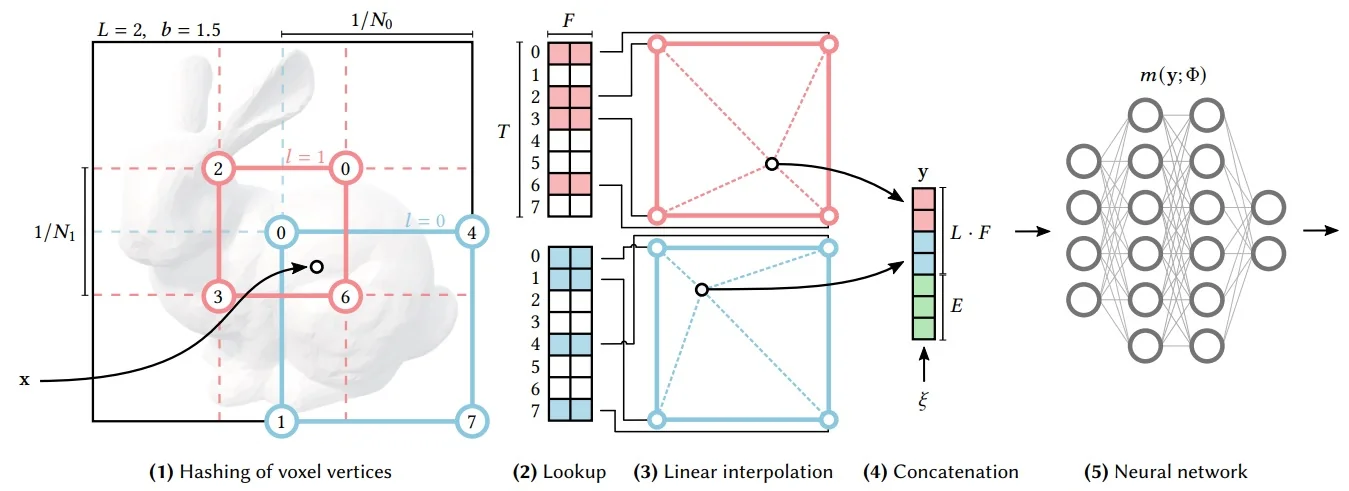
This architecture supports real-time training and rendering by combining a compact, hash-based spatial encoding with an extremely efficient neural decoder.
Occupancy Grid Acceleration To reduce the number of MLP evaluations in empty space, Instant-NGP employs a coarse occupancy grid that accelerates volume rendering by identifying which regions of the scene are likely to contain nonzero density. This grid is dynamically updated during training and acts as a binary mask that allows rays to skip regions deemed empty, leading to speedups of \( 10\times \) to \( 100\times \) in large scenes.
The grid is a 3D bitfield over a coarse voxelization of the scene’s bounding volume. For any sample point along a camera ray, the renderer first checks the occupancy bit of the voxel containing the point. If the bit is unset (i.e., the region is marked as empty), the sample is skipped and the MLP is not queried. This drastically reduces redundant computation in free space and occluded volumes.
The occupancy grid is not static; it is updated periodically based on the current predictions of the model. Specifically, Instant-NGP maintains a separate floating-point density grid (not visible to the renderer) to accumulate raw density values over time. Every \( N \) training steps (e.g., \( N = 16 \)), the system performs the following update:
- 1.
- A set of candidate grid cells is selected for update, using a combination of uniform sampling and rejection sampling near occupied regions.
- 2.
- For each selected cell, a random 3D point \( \mathbf {x} \) within the cell is chosen.
- 3.
- The MLP is queried at \( \mathbf {x} \) to obtain its predicted volume density \( \sigma (\mathbf {x}) \).
- 4.
- The cell’s accumulated density value is updated by taking the maximum of the existing value and \( \sigma (\mathbf {x}) \).
- 5.
- The final occupancy bit is set if this value exceeds a threshold \( \epsilon \); otherwise, the cell remains marked as empty.
Importantly, the MLP is not evaluated at the eight corners of each voxel for this purpose. Instead, it is evaluated at a single random point within the cell, which is sufficient to detect occupied space due to the smoothness of the learned density field. This process ensures that the occupancy grid reflects the evolving geometry of the scene, pruning away empty regions while preserving regions with fine detail.
At rendering time, this grid enables efficient ray marching: rays are advanced in larger steps through empty regions and subdivided only when approaching occupied space. Combined with Instant-NGP’s compact encoding, this mechanism enables high-fidelity novel view synthesis at interactive frame rates.
Training and Inference Training follows the same NeRF paradigm: rays are sampled, feature vectors are encoded from hash tables, densities and colors are predicted, and volume rendering integrates them into pixel colors. The MSE loss is backpropagated through the entire system, including the hash table entries (which are learnable) and the MLP. During inference, the process is purely feed-forward and supports 100+ FPS rendering on modern GPUs.
- Speed and Efficiency: Instant-NGP achieves dramatic acceleration over prior NeRF methods. With hash-based encoding and optimized CUDA kernels, it reaches high-quality reconstructions in just seconds. For example, on the LEGO scene, Instant-NGP matches or surpasses NeRF’s performance (\(32.54\) PSNR) in under 15 seconds of training (see the below table). Real-time rendering is also enabled at over 60 FPS.
- Quality and Convergence: Despite its speed, Instant-NGP does not sacrifice fidelity. After just 1 minute of training, it consistently outperforms NeRF [442] and NSVF [379], and achieves results competitive with or exceeding mip-NeRF [29]. Notably, the hash-encoded model reaches \(33.18\) average PSNR in 5 minutes—higher than all baselines.
- Compactness: The hash encoding decouples memory consumption from scene resolution. Each level uses a fixed-size table of \( T \) feature vectors, yielding predictable memory use (e.g., \(2-8\) MB), regardless of spatial complexity.
- Adaptivity: Collisions in the hash tables are not explicitly resolved. Instead, gradient-based optimization allocates representational capacity where needed: voxels near surfaces or textures produce stronger gradients and dominate updates to shared entries. This enables the model to prioritize detail-rich regions while ignoring redundant space.
-
Limitations:
- Requires custom CUDA kernels and optimized memory layouts, limiting ease of deployment across platforms.
- Primarily suited for dense photometric supervision; extensions to sparse-view or semantic tasks are nontrivial.
- Hash collisions may introduce subtle artifacts in high-frequency regions.
| Method | Mic | Ficus | Chair | Hotdog | Materials | Drums | Ship | Lego | Avg. |
| Instant-NGP (Hash, 1s) | 26.09 | 21.30 | 21.55 | 21.63 | 22.07 | 17.76 | 20.38 | 18.83 | 21.20 |
| Instant-NGP (Hash, 5s) | 32.60 | 30.35 | 30.77 | 33.42 | 26.60 | 23.84 | 26.38 | 30.13 | 29.26 |
| Instant-NGP (Hash, 15s) | 34.76 | 32.26 | 32.95 | 35.56 | 28.25 | 25.23 | 28.56 | 33.68 | 31.41 |
| Instant-NGP (Hash, 1m) | 35.92 | 33.05 | 34.34 | 36.78 | 29.33 | 25.82 | 30.20 | 35.63 | 32.64 |
| Instant-NGP (Hash, 5m) | 36.22 | 33.51 | 35.00 | 37.40 | 29.78 | 26.02 | 31.10 | 36.39 | 33.18 |
| mip-NeRF (hours) | 36.51 | 33.29 | 35.14 | 37.48 | 30.71 | 25.48 | 30.41 | 35.70 | 33.09 |
| NSVF (hours) | 34.27 | 31.23 | 33.19 | 37.14 | 32.68 | 25.18 | 27.93 | 32.29 | 31.74 |
| NeRF (hours) | 32.91 | 30.13 | 33.00 | 36.18 | 29.62 | 25.01 | 28.65 | 32.54 | 31.01 |
| Instant-NGP (Freq., 1m) | 26.62 | 24.72 | 28.51 | 32.61 | 26.36 | 21.33 | 24.32 | 28.88 | 26.67 |
| Instant-NGP (Freq., 5m) | 31.89 | 28.74 | 31.02 | 34.86 | 28.93 | 24.18 | 28.06 | 32.77 | 30.06 |
Key insight: By replacing dense voxel grids with multiresolution hash encodings and using a fully fused MLP, Instant-NGP transforms NeRF into a memory-efficient and GPU-optimal rendering system capable of real-time operation.
Enrichment 23.10.4: Nerfacto: Merging Instant-NGP & NR Pipelines
Nerfacto [625] generalizes the Instant-NGP architecture into a more robust and modular neural rendering pipeline. It retains the core speed advantages of multiresolution hash encodings, but integrates a range of techniques from more expressive NeRF variants—including Mip-NeRF 360, NeRF-W, and Ref-NeRF—to support complex, real-world data. Developed within the Nerfstudio framework, Nerfacto prioritizes flexibility, semantic extensibility, and practical usability over raw speed alone.
At the core, Nerfacto still uses a hash-encoded MLP to map each sampled 3D point \( \mathbf {x} \in \mathbb {R}^3 \) and view direction \( \mathbf {d} \in \mathbb {S}^2 \) to a predicted color and density. Like Instant-NGP, it queries a multiresolution hash grid to produce a high-frequency encoding \( \mathbf {f}(\mathbf {x}) \), which is fed to a compact decoder network.
However, Nerfacto departs from Instant-NGP in three major ways:
- Proposal Network Sampling: Nerfacto improves ray efficiency by using a hierarchy of lightweight proposal networks—small hash-encoded MLPs—that predict coarse density distributions. These guide sample placement toward regions of likely scene content, reducing wasted queries and enhancing edge sharpness. This replaces the occupancy grid with a more learned, view-adaptive sampling strategy, similar to mip-NeRF 360.
- Hybrid Feature Fusion: In addition to 3D hash features, Nerfacto optionally fuses image-space features from 2D convolutional encoders. These image features can inject view-specific cues, aiding the model in tasks like relighting, semantic rendering, or pose correction. The final input to the MLP decoder is a concatenation of 3D features, view direction encodings, and (optionally) per-image appearance embeddings or 2D descriptors.
- Extended Output and Losses: Unlike Instant-NGP—which focuses solely on color and density prediction—Nerfacto supports multi-head outputs and diverse losses, including surface normals, depth supervision, semantic labels, or photometric consistency across views. This makes it suitable for real-world, unbounded scenes captured with noisy camera poses and lighting variation.
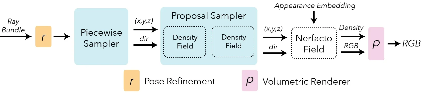
By combining fast hash-based encoding with modular losses, proposal sampling, and auxiliary inputs, Nerfacto enables real-time training and visualization even in messy, in-the-wild datasets. While Instant-NGP is best suited for clean, object-centric scenes with pre-registered cameras, Nerfacto handles general scenes with pose noise, dynamic lighting, and semantic supervision. It offers a practical middle ground between research flexibility and production deployment.
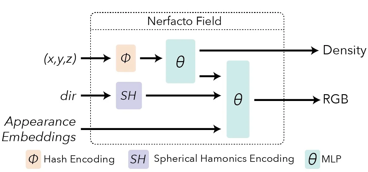
Applications and Design Goals Nerfacto is engineered not only for high-quality novel view synthesis, but also as a general-purpose backbone for a wide range of NeRF-style applications. Its modular design, efficient encoding, and support for auxiliary supervision make it suitable for both academic experimentation and real-world deployment. Key goals include:
- Reusability: Nerfacto supports downstream tasks such as relighting, surface extraction, and semantic segmentation. Fine-tuning is straightforward, enabling rapid adaptation to new scenes or objectives.
- Speed: By retaining Instant-NGP’s hash-based encoding and efficient volumetric rendering, Nerfacto preserves real-time training and inference speeds—despite additional model components and loss terms.
- Robustness: Nerfacto is designed to operate under imperfect capture conditions, including sparse viewpoints, noisy poses, and variable lighting. It generalizes well with minimal hyperparameter tuning and works effectively across both bounded and unbounded scenes.
Compared to Instant-NGP—which focuses on maximal efficiency for object-centric datasets with known poses—Nerfacto emphasizes extensibility and supervision-rich learning. Its architecture accommodates semantic objectives, auxiliary features, and dynamic inputs without sacrificing rendering quality or speed.
Core Insight and Tradeoffs Nerfacto’s core insight is that fast hash-based scene encoding can be extended into a flexible, semantically-aware rendering framework. The multiresolution hash grid compresses spatial variation across scales, while learned decoders map fused 3D and 2D features to rich volumetric outputs. This allows the model to achieve high fidelity with a compact parameter budget.
Although hash collisions are unavoidable at fine resolutions, their impact is mitigated by the multilevel encoding: even if two spatial positions collide at one resolution, they are unlikely to collide across all levels. This ensures that the final encoding \( \mathbf {f}(\mathbf {x}) \) remains discriminative and expressive, preserving sharp detail and accurate color prediction, just like in Instant-NGP.
Key insight: Nerfacto demonstrates that real-time neural rendering does not require sacrificing flexibility or supervision. By combining Instant-NGP’s memory efficiency with neural field modularity, it bridges efficient graphics pipelines and modern learning-based scene understanding.
Enrichment 23.10.5: TensoRF: Tensor-Factorized Fields
TensoRF [80] proposes a compact and interpretable alternative to MLP-based NeRF-style radiance field models. The scene is still represented as a continuous 5D function \[ \mathcal {F}(\mathbf {x}, \mathbf {d}) = (\sigma , \mathbf {c}), \] mapping a 3D location \( \mathbf {x} \in \mathbb {R}^3 \) and a viewing direction \( \mathbf {d} \in \mathbb {S}^2 \) to a scalar volume density \( \sigma \in \mathbb {R} \) and a view-dependent RGB color \( \mathbf {c} \in \mathbb {R}^3 \).
Overview Vanilla NeRF computes features by feeding spatial coordinates into a coordinate-based MLP, which is queried at every sampled point along a ray. TensoRF replaces this with an explicit, low-rank tensor representation that stores features in a structured form and can be queried directly via interpolation. This change shifts most computation from deep networks to simple lookups and lightweight decoding, reducing both memory and runtime while preserving compatibility with NeRF’s differentiable volume rendering framework. Conceptually, the model consists of:
- A 4D spatial feature tensor \( \mathcal {T} \in \mathbb {R}^{X \times Y \times Z \times C} \), storing a feature vector of dimension \(C\) at each spatial location \(\mathbf {x} = (x,y,z)\);
- A lightweight decoder \(S\) that maps features and a view direction \(\mathbf {d}\) to the density \(\sigma \) and RGB color \(\mathbf {c}\).
Radiance Field Decomposition via Tensor Approximation The latent feature field \(\mathcal {T}\) is decomposed into:
- Geometry tensor \( \mathcal {T}_\sigma \in \mathbb {R}^{X \times Y \times Z \times C_\sigma } \) — features used for density estimation.
- Appearance tensor \( \mathcal {T}_c \in \mathbb {R}^{X \times Y \times Z \times C_c} \) — features used for predicting view-dependent color.
These combine as \(\mathcal {T} = [\mathcal {T}_\sigma \;|\; \mathcal {T}_c]\) with \(C = C_\sigma + C_c\).
Rather than store \(\mathcal {T}\) densely, TensoRF learns a small number \(R = R_\sigma + R_c\) of axis-aligned vector–matrix (VM) factors, acting as compressed tensor components. For any point \(\mathbf {x} \in [0,1]^3\):
- Geometry features are reconstructed by summing \(R_\sigma \) geometry VM components.
- Appearance features are reconstructed by summing \(R_c\) appearance VM components.
- These are passed to density and color heads to compute \(\sigma (\mathbf {x})\) and \(\mathbf {c}(\mathbf {x}, \mathbf {d})\), respectively.
This factorization reduces storage complexity from \(\mathcal {O}(N^3 C)\) for a dense voxel grid to \(\mathcal {O}(N^2 R C)\), enabling high-resolution reconstructions without prohibitive memory costs.
Vector–Matrix (VM) Decomposition Each tensor field in TensoRF—whether the geometry tensor \( \mathcal {T}_\sigma \) or the appearance tensor \( \mathcal {T}_c \)—is not stored as a dense 4D grid. Instead, it is approximated using a sum of \( R \) low-rank vector–matrix (VM) components. For any continuous 3D query point \( \mathbf {x} = (x, y, z) \in [0,1]^3 \), each rank-\( r \) component evaluates as: \[ \hat {A}_r(\mathbf {x}) = v^{(x)}_r(x) \cdot M^{(y,z)}_r(y,z) + v^{(y)}_r(y) \cdot M^{(x,z)}_r(x,z) + v^{(z)}_r(z) \cdot M^{(x,y)}_r(x,y), \] where:
- \( v^{(i)}_r(\cdot ) \in \mathbb {R}^{N_i} \) is a learnable 1D vector defined along axis \( i \in \{x, y, z\} \), evaluated via linear interpolation.
- \( M^{(j,k)}_r(\cdot , \cdot ) \in \mathbb {R}^{N_j \times N_k} \) is a learnable 2D matrix over the orthogonal plane \( (j,k) \), evaluated via bilinear interpolation.
Each term behaves like a 3D slab: a vector modulates variation along one axis while the matrix textures the perpendicular plane. This makes VM components far more expressive than CP decomposition’s fully separable outer products, enabling detailed structures such as diagonal surfaces or 2D textures with fewer components.
Interpolation: From Discrete Grids to Continuous Coordinates TensoRF learns vector and matrix values at discrete grid locations (e.g., \( N_x = 128 \) entries along the x-axis), but rendering requires evaluating them at continuous 3D coordinates. This is achieved by differentiable interpolation:
1. Normalization. All 3D sample points are first mapped from world coordinates into the normalized unit cube \( [0,1]^3 \) that encloses the scene. If a ray exits this cube, integration stops and no further queries are made.
2. Linear interpolation (1D vectors). For a coordinate \( x \in [0,1] \) and vector \( v^{(x)}_r \in \mathbb {R}^{N_x} \), we: \[ u = x \cdot (N_x - 1), \quad i = \lfloor u \rfloor , \quad \alpha = u - i, \] \[ v^{(x)}_r(x) = (1 - \alpha ) \cdot v^{(x)}_r[i] + \alpha \cdot v^{(x)}_r[i+1]. \] This blends the two neighboring entries based on the fractional offset \( \alpha \). If \( x \) aligns with a grid cell center (e.g., \( \alpha = 0 \)), it degenerates to a direct lookup.
3. Bilinear interpolation (2D matrices). For a matrix \( M^{(y,z)}_r \in \mathbb {R}^{N_y \times N_z} \) and normalized coordinates \( (y, z) \in [0,1]^2 \): \[ u = y \cdot (N_y - 1), \quad v = z \cdot (N_z - 1), \] \[ i = \lfloor u \rfloor , \quad j = \lfloor v \rfloor , \quad \alpha = u - i, \quad \beta = v - j, \] \[ \begin {aligned} M^{(y,z)}_r(y,z) =\; & (1-\alpha )(1-\beta ) \cdot M[i,j] + \alpha (1-\beta ) \cdot M[i+1,j] \\ +& (1-\alpha )\beta \cdot M[i,j+1] + \alpha \beta \cdot M[i+1,j+1]. \end {aligned} \]
Example. Suppose \( x = 0.5 \), and \( N_x = 128 \). Then \( u = 63.5 \), so we interpolate between \( v_r^{(x)}[63] \) and \( v_r^{(x)}[64] \) with equal weights. If \( y = 0.7 \), \( z = 0.2 \), and \( N_y = N_z = 128 \), we blend the four matrix entries around cell \( (89, 25) \) according to the local offsets \( \alpha \), \( \beta \).
Differentiability and Training Efficiency Since linear and bilinear interpolation are piecewise-linear functions of \( \mathbf {x} \), gradients propagate through them during backpropagation. This enables end-to-end training of all vector and matrix values using volume rendering loss, just like weights in a neural network.
VM decomposition thus achieves a balance between expressiveness and efficiency. Each axis-aligned component requires only a small number of memory lookups (2 for vectors, 4 for matrices), and scales quadratically in spatial resolution rather than cubically like voxel grids. This makes TensoRF compact, fast, and differentiable, with no need for deep MLPs at inference time.
Geometry: View-Independent Density Estimation To compute the scalar volume density at a query point \( \mathbf {x} \in [0,1]^3 \), TensoRF evaluates all geometry VM components and linearly combines them using learned scalar weights \( w^{(\sigma )}_r \). This sum is then passed through a shifted Softplus activation: \[ \sigma (\mathbf {x}) = \log \left (1 + \exp \left (\sum _{r=1}^{R_\sigma } w^{(\sigma )}_r \cdot \hat {A}_{\sigma ,r}(\mathbf {x}) + \beta \right )\right ), \] where \( \beta \in \mathbb {R} \) is a learned bias.
This decoder-free formulation directly outputs a non-negative scalar density without using a neural network. The Softplus function, defined as \[ \texttt{Softplus}(z) = \log (1 + \exp (z)), \] smoothly approximates the ReLU function and ensures that the predicted density is always positive. The shifted variant \( \texttt{Softplus}(z + \beta ) \) improves training stability and expressiveness.
Appearance: View-Dependent Color Prediction To model view-dependent color, TensoRF uses a separate set of VM components. Each component \( r \in \{1, \ldots , R_c\} \) contributes a 3D appearance feature vector at point \( \mathbf {x} \), constructed by concatenating the outputs from its three axis–plane interactions: \[ \mathbf {f}_c^{(r)}(\mathbf {x}) = \left [ v^{(x)}_r(x) M^{(y,z)}_r(y,z), \quad v^{(y)}_r(y) M^{(x,z)}_r(x,z), \quad v^{(z)}_r(z) M^{(x,y)}_r(x,y) \right ]. \]
The full appearance descriptor is then computed by summing over all such components: \[ \mathbf {f}_c(\mathbf {x}) = \sum _{r=1}^{R_c} \mathbf {f}_c^{(r)}(\mathbf {x}) \in \mathbb {R}^{C_c}. \]
This feature vector is projected using a learned matrix \( B \in \mathbb {R}^{P \times C_c} \), where \( P \) is the number of latent appearance channels used by the color decoder. The projected feature is combined with a frequency-encoded view direction \( \mathbf {s}(\mathbf {d}) \), and passed to a lightweight decoder \( S \): \[ \mathbf {c}(\mathbf {x}, \mathbf {d}) = S\left ( B \cdot \mathbf {f}_c(\mathbf {x}),\; \mathbf {s}(\mathbf {d}) \right ). \]
The decoder \( S \) is typically a two-layer MLP or a small set of spherical harmonic (SH) basis functions. This architecture enables efficient modeling of view-dependent lighting and appearance while maintaining fast inference.
Comparison to CP Decomposition TensoRF also explores a CP (CANDECOMP/PARAFAC) decomposition of the form: \[ \mathcal {T}(x, y, z) = \sum _{r=1}^R v^{(x)}_r(x) \cdot v^{(y)}_r(y) \cdot v^{(z)}_r(z), \] where each rank-\( r \) term is the outer product of three 1D vectors defined along the spatial axes. This formulation is highly compact, requiring only \( \mathcal {O}(N R) \) memory for resolution \( N \), but suffers from a strong separability constraint: each component captures only rank-1 correlations across the three dimensions. As a result, it lacks the capacity to model complex structures such as depth discontinuities, slanted edges, or fine textures, unless the rank \( R \) is increased substantially.
In contrast, the vector–matrix (VM) decomposition adopted in TensoRF breaks this constraint by coupling two spatial axes per term. Each component \( \hat {A}_r(\mathbf {x}) \) includes bilinear interaction over a 2D matrix (e.g., \( y \)-\( z \)) modulated by variation along the third axis (e.g., \( x \)). This allows a single VM component to encode high-frequency planar details or axis-aligned surface patterns that would require many CP terms to approximate.
Mathematically, the VM decomposition relaxes the strict separability constraint of CP by modeling 2D spatial interactions explicitly through matrix components. This increases the expressive power of each rank-\( r \) term while preserving a tractable memory footprint of \( \mathcal {O}(N^2 R) \), significantly more scalable than dense voxel grids yet more flexible than rank-1 CP.
Empirically, this design enables TensoRF-VM to achieve superior tradeoffs between accuracy, efficiency, and compactness. The model converges rapidly—typically within a few to tens of minutes—while attaining higher PSNR than both CP-based variants and dense-grid baselines. Furthermore, its compact factorized representation yields scene models as small as 30–75MB that match or exceed the visual fidelity of MLP-based NeRFs, with real-time rendering performance and substantially reduced parameter count.
Summary TensoRF’s VM decomposition reframes 3D scene representation as a problem in efficient multilinear algebra. It enables fast, continuous queries, low memory usage, and real-time rendering without relying on deep MLPs. The combination of geometry and appearance factorization into interpretable, axis-aligned vector–matrix components provides both practical acceleration and theoretical insight into compact neural field design.
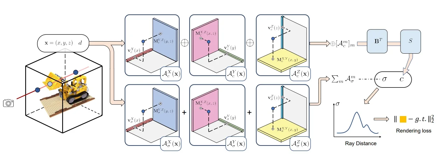
Quantitative Comparison TensoRF achieves excellent reconstruction quality while offering faster training and reduced memory. The following table compares TensoRF against major baselines on standard NeRF benchmarks, including Synthetic-NeRF, NSVF, and Tanks & Temples:
| Method | Time | Size (MB) | Synthetic-NeRF | NSVF | Tanks & Temples
| |||
|---|---|---|---|---|---|---|---|---|
| PSNR↑ | SSIM↑ | PSNR↑ | SSIM↑ | PSNR↑ | SSIM↑ | |||
| NeRF [442] | 35h | 5.0 | 31.01 | 0.947 | 30.81 | 0.952 | 25.78 | 0.864 |
| NSVF [379] | \(>\)48h | - | 31.75 | 0.953 | 35.18 | 0.979 | 28.48 | 0.901 |
| Plenoxels [162] | 11.4m | 778.1 | 31.71 | 0.958 | - | - | 27.43 | 0.906 |
| DVGO [613] | 15.0m | 612.1 | 31.95 | 0.957 | 35.08 | 0.975 | 28.41 | 0.911 |
| TensoRF (VM-192) | 17.4m | 71.8 | 33.14 | 0.963 | 36.52 | 0.982 | 28.56 | 0.920 |
Qualitative Results As shown in the below figure, TensoRF produces sharp, photorealistic reconstructions with accurate geometry and appearance. Notably, it recovers fine details such as the floor and shadows in synthetic scenes more faithfully than NeRF or Plenoxels, and exhibits fewer aliasing artifacts.
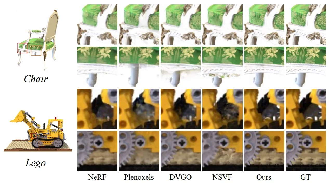
Key insight: TensoRF shows that tensor decomposition offers a memory-efficient and accurate alternative to MLP-heavy or voxel-based radiance field models. By factorizing spatial variation into 1D and 2D components, it achieves state-of-the-art results with significantly reduced overhead.
Enrichment 23.10.6: Mip-NeRF: Anti-Aliased Radiance Fields
Motivation: scale ambiguity and aliasing In standard NeRF [442], each pixel is modeled as a single, infinitesimally thin ray, even though in reality a pixel sees a finite footprint in the scene. This footprint corresponds to a cone-shaped region of space whose size grows with depth. When training with mixed-scale imagery (both close-up and distant views), NeRF’s point-sampled positional encoding ignores the footprint size entirely, forcing the network to reconcile incompatible signals.
Without scale awareness, two characteristic artifacts appear:
- Aliasing in distant views: A faraway pixel’s footprint may intersect fine geometry that is smaller than the pixel can resolve. Sampling only at its center captures spurious high-frequency detail, producing jagged edges or temporal shimmer.
- Over-smoothing in close-up views: To remain consistent with coarse, distant observations, the model suppresses fine detail in close-ups, leading to blurriness and loss of texture.
While supersampling (casting multiple rays per pixel) can reduce both problems by averaging over the footprint, it does not guarantee perfect removal of aliasing and is prohibitively expensive — each extra ray multiplies the number of MLP evaluations.
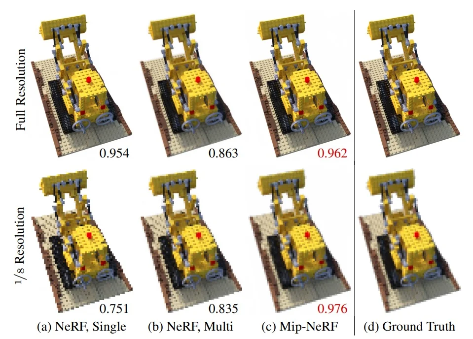
From pixels to cones In a real pinhole camera, a pixel does not capture light from a single infinitesimal ray, but from a continuous bundle of rays passing through its finite footprint on the image plane. These rays form a cone whose apex is at the camera center and whose axis points through the pixel center. The further we travel along this cone into the scene, the larger its cross-section becomes — so the same pixel may correspond to a tiny region on a nearby surface but a much larger region on a distant one. To model a pixel’s contribution faithfully, we therefore need to account for how both the position and the spatial extent of the region it covers change with depth, setting the stage for a depth-wise decomposition of the cone.
Why cones are divided into frustums In volumetric rendering, the color of a pixel is obtained by integrating scene density and radiance along the corresponding camera ray. For a cone-shaped pixel footprint, doing this integration over the entire cone in one step is both impractical and physically inaccurate:
- Depth variation: The scene’s density and emitted color change continuously with depth.
- Occlusion: Objects at different distances can block each other, so visibility changes along the viewing direction.
- Light transport: The transmittance — the fraction of light that reaches the camera — must be updated incrementally as we progress through space.
If we treated the entire cone as a single unit, these effects would be averaged together indiscriminately, erasing important depth-dependent structure.
The remedy is to discretize the cone into a sequence of depth intervals \[ [t_0, t_1], \; [t_1, t_2], \; \dots , \] each forming a frustum — the portion of the cone between two depth planes. This is conceptually similar to NeRF’s point sampling along a ray, but instead of single points, each sample now represents a finite 3D region with a nonzero cross-section. By working with frustums, we can:
- Associate each segment with its own spatial footprint size, enabling scale-aware encoding.
- Capture how density, color, and visibility change between consecutive depth ranges.
- Incrementally update transmittance and accumulate contributions in a physically consistent manner.
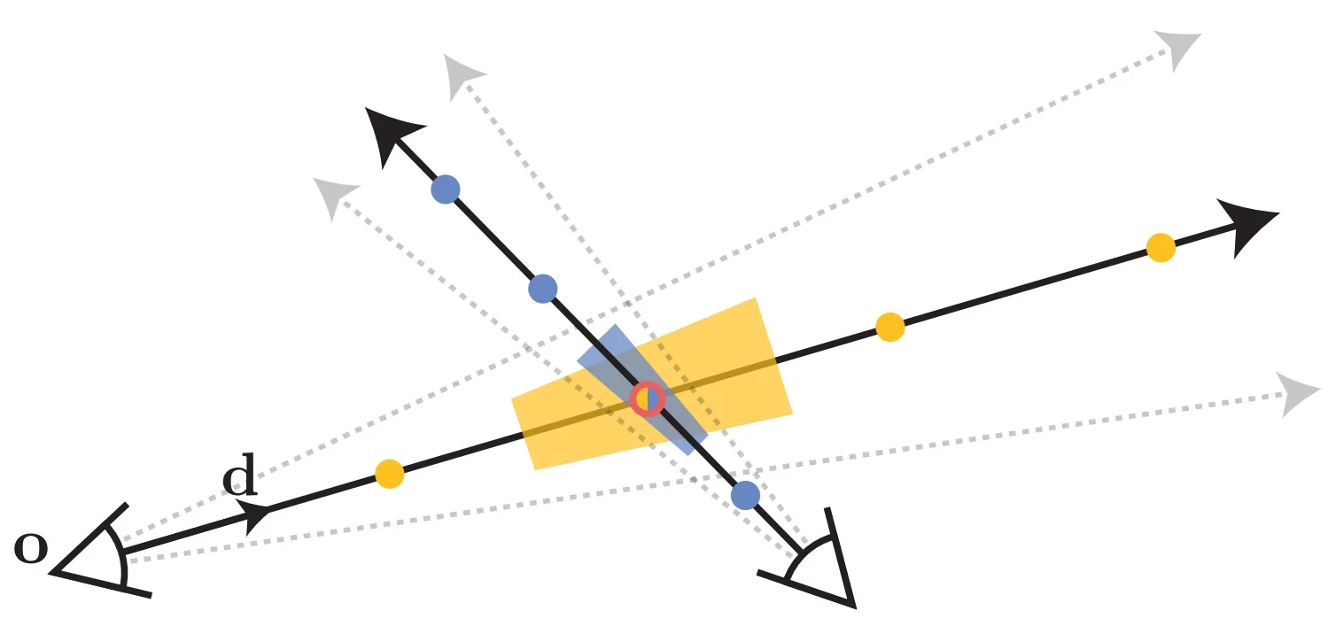
From frustums to a pixel’s color Once the cone is split into frustums, the rendering process accumulates their contributions to produce the final pixel value. For the \(k\)-th frustum, the network predicts a mean density \(\sigma _k\) and a mean color \(\mathbf {c}_k\) that represent the frustum’s aggregated appearance. These are then combined using the standard volume rendering equation: \[ C_{\mbox{pixel}} = \sum _{k=1}^N T_k \, \alpha _k \, \mathbf {c}_k , \] where:
- \(\alpha _k = 1 - \exp (-\sigma _k \, \Delta t_k)\) is the frustum’s opacity given its depth thickness \(\Delta t_k\),
- \(T_k = \prod _{j=1}^{k-1} (1 - \alpha _j)\) is the transmittance — the fraction of light that reaches frustum \(k\) without being blocked by earlier segments.
This discrete summation mirrors NeRF’s point-based accumulation but replaces points with scale-aware volumetric regions.
Crucially, unlike the original NeRF [442], which applies positional encoding to a single 3D point along each ray sample, Mip-NeRF instead asks:
What is the average positional encoding of all points within this frustum?
Here, “positional encoding” refers to the same Fourier feature mapping used in NeRF to represent high-frequency variation in color and density. Averaging these features over the frustum volume acts as a principled low-pass filter: sub-frustum spatial variation is integrated out, while coarser structure is preserved. This transforms each sample into a scale-aware volumetric descriptor rather than a potentially aliased point measurement.
From pixels to cones In the pinhole camera model, a pixel corresponds not to a single infinitesimal ray, but to the set of rays passing through its finite footprint on the image plane. These rays form a cone with apex at the camera center \( \mathbf {o} \in \mathbb {R}^3 \) and central axis along the unit ray direction \( \mathbf {d} \in \mathbb {R}^3 \) through the pixel center.
At a depth \(t\) along \(\mathbf {d}\), the cone’s cross-section is the back-projection of the pixel’s footprint into 3D space. If the pixel is square with width \(w\) (in world-space units at the image plane) and the camera has focal length \(f\) (same units), similar triangles show that this cross-section is a square whose side length—the physical distance between two opposite edges—is: \[ S(t) = \frac {w}{f} \, t. \] At unit depth (\(t=1\)), this reduces to \(S = \frac {w}{f}\), the side length of the footprint in world units when projected to 1 meter from the camera.
Approximating the footprint as a disk To simplify later analytic derivations, Mip-NeRF replaces the square cross-section at each depth with a rotationally symmetric disk of radius \(r(t)\), producing a right circular cone. If we simply took \(r(t) = S(t)/2\) so the disk matched the square’s width, the two shapes would differ in their second moments (spatial variances), meaning they would have different frequency responses and thus different effective blur sizes.
To ensure the disk has the same spatial spread as the square, Mip-NeRF uses variance matching. For a shape centered at the origin, the marginal variance along one axis is: \[ \mathrm {Var}_{\mbox{square}} = \frac {S^2}{12}, \qquad \mathrm {Var}_{\mbox{disk}} = \frac {R^2}{4}, \] where \(S\) is the square’s side length and \(R\) is the disk’s radius. Equating these variances: \[ \frac {S^2}{12} = \frac {R^2}{4} \quad \Rightarrow \quad R = \frac {S}{\sqrt {3}}. \]
Thus the matched disk radius at depth \(t\) is: \[ r(t) = \frac {S(t)}{\sqrt {3}} = \frac {w}{f \sqrt {3}} \, t, \] so the radius grows linearly with depth with slope \[ \dot {r} = \frac {w}{f\sqrt {3}}, \] representing the disk radius per unit depth.
Why variance matching? Variance measures the average squared distance of footprint points from its center, directly controlling the degree of spatial smoothing. Matching variances ensures that the simplified disk and the true square blur high-frequency detail in the same way, while the disk’s rotational symmetry allows later analytic treatment of frustums. This makes it possible for Mip-NeRF to replace costly Monte Carlo integration with closed-form Gaussian-based anti-aliasing in subsequent steps.
Frustum geometry and indicator function To formalize this region of space, Mip-NeRF defines an indicator function \[ \mathrm {F}(\mathbf {x}, \mathbf {o}, \mathbf {d}, \dot {r}, t_0, t_1), \] which returns \( 1 \) if a 3D point \( \mathbf {x} \in \mathbb {R}^3 \) lies inside the conical frustum defined by origin \( \mathbf {o} \), axis \( \mathbf {d} \), slope \( \dot {r} \), and depth bounds \( t_0, t_1 \), and \( 0 \) otherwise: \begin {equation} \mathrm {F}(\mathbf {x}, \mathbf {o}, \mathbf {d}, \dot {r}, t_0, t_1) = \mathbb {1} \left \{ \left ( t_0 < \frac {\mathbf {d}^\top (\mathbf {x} - \mathbf {o})}{\|\mathbf {d}\|_2^2} < t_1 \right ) \land \left ( \frac {\mathbf {d}^\top (\mathbf {x} - \mathbf {o})}{\|\mathbf {d}\|_2 \, \|\mathbf {x} - \mathbf {o}\|_2} > \frac {1}{\sqrt {1 + (\dot {r} / \|\mathbf {d}\|_2)^2}} \right ) \right \}. \label {eq:chapter23_mipnerf_indicator} \end {equation}
This condition performs two geometric checks:
-
Depth check: The term \[ \frac {\mathbf {d}^\top (\mathbf {x} - \mathbf {o})}{\|\mathbf {d}\|^2} \in (t_0, t_1) \] measures how far along the ray axis the projection of \( \mathbf {x} \) lies. Here:
- \( \mathbf {x} - \mathbf {o} \) is the displacement from the ray origin.
- The dot product \( \mathbf {d}^\top (\mathbf {x} - \mathbf {o}) \) gives the scalar projection of this displacement onto \( \mathbf {d} \).
- Division by \( \|\mathbf {d}\|^2 \) converts this projection into a true depth value even if \( \mathbf {d} \) is not unit length.
The inequality enforces that the point lies between the near and far depth planes of the frustum.
-
Angular check: This condition tests whether the point \(\mathbf {x}\) lies inside the angular aperture of the cone defined by the pixel footprint.
First, recall that the vector \(\mathbf {d}\) is the central ray direction of the cone, and \(\mathbf {x} - \mathbf {o}\) is the vector from the camera origin to the point \(\mathbf {x}\). The angle between these two vectors is: \[ \theta = \angle (\mathbf {d}, \mathbf {x} - \mathbf {o}), \] whose cosine can be computed via the dot product: \[ \cos (\theta ) = \frac {\mathbf {d}^\top (\mathbf {x} - \mathbf {o})}{\|\mathbf {d}\| \, \|\mathbf {x} - \mathbf {o}\|}. \]
The cone’s half-angle \(\alpha \) is the angular radius of its cross-section as seen from the apex. From the slope definition \(\dot {r}\) (radius per unit depth), we have: \[ \tan (\alpha ) = \frac {\dot {r}}{\|\mathbf {d}\|}, \] and therefore: \[ \cos (\alpha ) = \frac {1}{\sqrt {1 + (\dot {r} / \|\mathbf {d}\|)^2}}. \]
The check: \[ \frac {\mathbf {d}^\top (\mathbf {x} - \mathbf {o})}{\|\mathbf {d}\| \, \|\mathbf {x} - \mathbf {o}\|} > \frac {1}{\sqrt {1 + (\dot {r} / \|\mathbf {d}\|)^2}} \] is equivalent to testing: \[ \cos (\theta ) > \cos (\alpha ). \]
Since \(\cos (\theta )\) decreases monotonically with \(\theta \) over the range \([0, \pi ]\), the inequality \(\cos (\theta ) > \cos (\alpha )\) means: \[ \theta < \alpha . \] In words: the angular deviation of \(\mathbf {x}\) from the cone axis is smaller than the cone’s half-angle, so \(\mathbf {x}\) lies within the cone’s aperture rather than outside it.
Why this matters: The frustum is defined not only by near and far depth limits along the axis, but also by the cone’s angular extent. Even if a point lies between \(t_0\) and \(t_1\) in depth, it must also pass this angular check to ensure it projects back to the same pixel footprint on the image plane. Without this test, the frustum definition would include points that are too far off-axis to be observed through the pixel.
Together, these checks precisely describe the 3D frustum volume subtended by a pixel over a given depth range. With this exact region defined, Mip-NeRF can next express the expected positional encoding over the frustum as a normalized volume integral—providing the starting point for the derivation that follows.
Expected positional encoding over a frustum Given the frustum region described by the indicator function \(\mathrm {F}\) from (23.1), Mip-NeRF defines the expected positional encoding as the mean of the NeRF positional encoding \(\gamma (\mathbf {x})\) over all 3D points \(\mathbf {x}\) lying within the frustum.
Formally, let \(\mathbf {X}\) be a random point drawn uniformly from the frustum volume \[ R = \{ \mathbf {x} \in \mathbb {R}^3 \mid \mathrm {F}(\mathbf {x}, \mathbf {o}, \mathbf {d}, \dot {r}, t_0, t_1) = 1 \}. \] The uniform density on \(R\) is \[ p(\mathbf {x}) \;=\; \frac {1}{\mathrm {Vol}(R)} \, \mathbb {1}_R(\mathbf {x}), \quad \mathrm {Vol}(R) = \int _{\mathbb {R}^3} \mathbb {1}_R(\mathbf {x}) \, d\mathbf {x}. \] The expectation of \(\gamma (\mathbf {X})\) under \(p\) is therefore \[ \mathbb {E}[\gamma (\mathbf {X})] = \int _{\mathbb {R}^3} \gamma (\mathbf {x})\, p(\mathbf {x})\, d\mathbf {x} = \frac {1}{\mathrm {Vol}(R)} \int _{R} \gamma (\mathbf {x}) \, d\mathbf {x}. \] Substituting the frustum indicator \(\mathrm {F}\) for \(\mathbb {1}_R\) gives \begin {equation} \gamma ^*(\mathbf {o}, \mathbf {d}, \dot {r}, t_0, t_1) = \frac { \int _{\mathbb {R}^3} \gamma (\mathbf {x}) \, \mathrm {F}(\mathbf {x}, \mathbf {o}, \mathbf {d}, \dot {r}, t_0, t_1) \, d\mathbf {x} }{ \int _{\mathbb {R}^3} \mathrm {F}(\mathbf {x}, \mathbf {o}, \mathbf {d}, \dot {r}, t_0, t_1) \, d\mathbf {x} }. \label {eq:chapter23_mipnerf_expected_encoding} \end {equation}
Here:
- The denominator is the frustum’s volume — the total measure of all 3D points that project to the given pixel between depths \(t_0\) and \(t_1\).
- The numerator integrates the encoded feature vector \(\gamma (\mathbf {x})\) over exactly the same set of points.
Their ratio is thus the uniform average of \(\gamma (\mathbf {x})\) over the frustum.
Intuition The expected positional encoding in (23.2) is the uniform average of \(\gamma (\mathbf {x})\) over the frustum \(R\). Formally, if \(\mathbf {x} \sim \mathrm {Uniform}(R)\), then \[ \mathbb {E}[\gamma (\mathbf {x})] = \frac {1}{\mathrm {Vol}(R)} \int _{R} \gamma (\mathbf {x}) \; d\mathbf {x}. \] In the discrete case, this would be approximated as \[ \frac {1}{N} \sum _{i=1}^N \gamma (\mathbf {x}_i), \quad \mathbf {x}_i \stackrel {\mbox{i.i.d.}}{\sim } \mathrm {Uniform}(R), \] and taking \(N \to \infty \) recovers the continuous form above. The denominator in (23.2) normalizes the numerator, converting it from a total sum over space into a mean per unit volume.
In the original NeRF formulation, each pixel is represented by a single infinitesimally narrow ray, so \(\gamma (\mathbf {x})\) is evaluated only along that 1D path. This ignores the fact that a real pixel integrates light over a finite footprint on the image plane, corresponding to a continuum of rays forming a conical frustum in 3D space. Mip-NeRF instead averages \(\gamma (\mathbf {x})\) over this entire frustum, embedding the pixel’s full visual support directly into its feature vector.
This volumetric averaging acts as a built-in low-pass filter. If the wavelength of a sinusoidal component in \(\gamma (\mathbf {x})\) is smaller than the frustum’s cross-section, its oscillations average out, attenuating high-frequency terms that would otherwise cause aliasing when rendering at resolutions or viewing distances different from training. Frequencies with wavelengths larger than the frustum remain unaffected, preserving resolvable detail. The result is scale consistency: textures that are smooth at a distance will not develop spurious high-frequency artifacts up close, and fine details will naturally fade with distance rather than alias into incorrect patterns.
A straightforward way to compute the average in (23.2) is to approximate it via Monte Carlo sampling: draw points uniformly inside the frustum and average their encodings. While conceptually simple, this approach is inefficient in practice:
- High variance: Monte Carlo estimates fluctuate due to sampling noise, especially for the high-frequency sinusoidal terms in \(\gamma (\mathbf {x})\).
- Computational cost: Achieving stable, low-variance estimates requires many samples per pixel, inflating training and rendering time.
- Missed structure: The positional encoding \(\gamma (\mathbf {x})\) is composed of sinusoidal basis functions, whose integrals over certain geometric shapes can be computed exactly.
To avoid stochastic approximation entirely, Mip-NeRF replaces each frustum segment with a moment-matched Gaussian distribution \(\mathcal {N}(\boldsymbol {\mu }, \boldsymbol {\Sigma })\) that has the same first and second moments as the true frustum. This substitution retains the key spatial statistics while making the expected positional encoding \(\mathbb {E}[\gamma (\mathbf {X})]\) analytically tractable. With this Gaussian model in place, the integral in (23.2) reduces to closed-form expressions for the mean and covariance of \(\mathbf {X}\).
Moment-matched Gaussian approximation To enable closed-form evaluation of (23.2), Mip-NeRF replaces the uniform distribution over a frustum segment with a Gaussian \(\mathcal {N}(\boldsymbol {\mu }, \boldsymbol {\Sigma })\) having the same first and second moments. The idea is that the frustum is a truncated cone whose geometry is simple enough that we can compute these moments analytically, and then replace the frustum with a Gaussian of matching mean and covariance.
Frustum-centric coordinates We first align our coordinate system so that the ray direction is the \(t\)-axis: \[ \hat {\mathbf {d}} = \frac {\mathbf {d}}{\|\mathbf {d}\|}, \qquad \mathbf {x}(t, \mathbf {u}) = \mathbf {o} + t\,\hat {\mathbf {d}} + \mathbf {u}, \] where:
- \(t \in [t_0, t_1]\) is the depth along the ray,
- \(\mathbf {o} \in \mathbb {R}^3\) is the ray origin,
- \(\mathbf {u} \in \mathbb {R}^3\) is a vector perpendicular to \(\hat {\mathbf {d}}\).
The frustum’s circular cross-section at depth \(t\) has radius \[ r(t) = \dot {r}\,t, \] where \(\dot {r}\) is the cone’s angular radius in world units (essentially the pixel footprint’s half-width projected into 3D space).
Marginal depth distribution \(p(t)\) A key step in Mip-NeRF’s Gaussian frustum approximation is to characterize the depth distribution of points within a pixel’s 3D footprint. For a given pixel, this footprint is modeled as a right circular cone originating at the camera center \(\mathbf {o}\) and extending along the viewing ray. The cone has slope \(\dot r\) (radius per unit depth), chosen to match the pixel’s footprint on the image plane.
At a distance \(t\) from \(\mathbf {o}\) along the ray, the cone’s cross–section is a disk of radius \[ r(t) = \dot r\,t, \] and therefore exact area \[ A(t) = \pi \,[r(t)]^2 = \pi \,(\dot r\,t)^2. \] A thin slab between depths \(t\) and \(t+dt\) has volume element \[ dV(t) = A(t)\,dt = \pi \,(\dot r)^2\,t^2\,dt. \]
The uniform-in-volume assumption means that the probability of sampling a point in a slab is proportional to its volume. Deeper slabs have larger cross–sections and therefore more 3D volume per unit depth. Taking the unnormalized marginal depth density to be the actual slice area gives \[ p_{\mbox{unnorm}}(t) = \pi \,(\dot r)^2\,t^2, \qquad t \in [t_0, t_1], \] where \(t_0\) and \(t_1\) are the near and far bounds of the frustum segment.
To convert \(p_{\mbox{unnorm}}(t)\) into a probability density, we divide by its total mass over \([t_0,t_1]\): \[ p(t) = \frac {p_{\mbox{unnorm}}(t)}{\displaystyle \int _{t_0}^{t_1} p_{\mbox{unnorm}}(\tau )\,d\tau } = \frac {\pi (\dot r)^2\,t^2}{\displaystyle \int _{t_0}^{t_1} \pi (\dot r)^2\,\tau ^2\,d\tau } = \frac {t^2}{\displaystyle \int _{t_0}^{t_1} \tau ^2\,d\tau }. \] The geometric constants \(\pi \) and \((\dot r)^2\) cancel exactly, so no arbitrary constant \(C\) must be introduced.
Evaluating the remaining denominator: \[ \int _{t_0}^{t_1} \tau ^2\,d\tau = \left [ \frac {\tau ^3}{3} \right ]_{t_0}^{t_1} = \frac {t_1^3 - t_0^3}{3}, \] yields the closed form \[ p(t) = \frac {3\,t^2}{t_1^3 - t_0^3}, \qquad t \in [t_0, t_1]. \]
This density is the correct marginal for uniform-in-volume sampling, and is later used to compute the mean depth \(\mu _t\) and depth variance \(\sigma _t^2\) of the Gaussian frustum. By contrast, weighting by \(1/A(t)\) would correspond to sampling uniformly along the axis, giving each depth slice equal probability regardless of its volume—an assumption inconsistent with volumetric pixel modeling.
Mean depth \(\mu _t\) In probability theory, the mean (expected) value of a continuous random variable \(t\) with probability density function (PDF) \(p(t)\) is \begin {equation} \mu _t \;=\; \mathbb {E}[t] \;=\; \int _{t_0}^{t_1} t \, p(t) \, dt. \label {eq:chapter23_mipnerf_expectation_def} \end {equation} In our frustum setting, the marginal depth density \(p(t)\) is proportional to the cross-sectional area at depth \(t\), which grows as \(t^2\) for a cone. Normalizing over \([t_0, t_1]\) yields \[ p(t) = \frac {3\,t^2}{t_1^3 - t_0^3}, \qquad t \in [t_0, t_1]. \] Substituting into Eq. 23.3: \begin {align} \mu _t &= \frac {3}{t_1^3 - t_0^3} \int _{t_0}^{t_1} t^3 \, dt = \frac {3}{t_1^3 - t_0^3} \left [ \frac {t^4}{4} \right ]_{t_0}^{t_1} \\ &= \frac {3\,(t_1^4 - t_0^4)}{4\,(t_1^3 - t_0^3)}. \label {eq:chapter23_mipnerf_mu_t_exact} \end {align}
Why not the midpoint? If \(p(t)\) were uniform, the mean would be \((t_0 + t_1)/2\). Here, \(p(t) \propto t^2\) upweights deeper slices because they occupy more volume, shifting \(\mu _t\) toward \(t_1\).
Stable reparameterization of \(\mu _t\) When \(t_1 \approx t_0\), Eq. (23.67) can suffer from catastrophic cancellation. To avoid this, define \[ t_\mu = \frac {t_0 + t_1}{2}, \qquad t_\delta = \frac {t_1 - t_0}{2}, \] so that \(t_0 = t_\mu - t_\delta \) and \(t_1 = t_\mu + t_\delta \). Using the binomial expansions \[ (t_\mu + t_\delta )^3 - (t_\mu - t_\delta )^3 = 6\,t_\mu ^2\,t_\delta + 2\,t_\delta ^3, \] \[ (t_\mu + t_\delta )^4 - (t_\mu - t_\delta )^4 = 8\,t_\mu ^3\,t_\delta + 8\,t_\mu \,t_\delta ^3, \] Eq. (23.4) simplifies to \begin {equation} \mu _t = t_\mu \;+\; \frac {2\,t_\mu \,t_\delta ^2}{3t_\mu ^2 + t_\delta ^2}, \label {eq:chapter23_mipnerf_mu_t_stable} \end {equation} which is exactly the mean formula in the Mip-NeRF paper.
Axial variance \(\sigma _t^2\) The variance along the ray is \begin {equation} \sigma _t^2 \;=\; \mathbb {E}[t^2] - \mu _t^2, \label {eq:chapter23_mipnerf_axial_variance} \end {equation} where the second moment is \begin {align} \mathbb {E}[t^2] &= \frac {3}{t_1^3 - t_0^3} \int _{t_0}^{t_1} t^4 \, dt = \frac {3}{t_1^3 - t_0^3} \left [ \frac {t^5}{5} \right ]_{t_0}^{t_1} \\ &= \frac {3\,(t_1^5 - t_0^5)}{5\,(t_1^3 - t_0^3)}. \label {eq:chapter23_mipnerf_second_moment_t} \end {align}
Stable reparameterization of \(\sigma _t^2\) Substitute \(t_\mu , t_\delta \) and use \[ (t_\mu + t_\delta )^5 - (t_\mu - t_\delta )^5 = 10\,t_\mu ^4\,t_\delta + 20\,t_\mu ^2\,t_\delta ^3 + 2\,t_\delta ^5, \] along with the cubic difference above, to obtain \[ \mathbb {E}[t^2] = \frac {3\,(t_\mu ^4 + 2\,t_\mu ^2\,t_\delta ^2 + \tfrac {1}{5}t_\delta ^4)} {3\,t_\mu ^2 + t_\delta ^2}. \] Similarly, squaring Eq. 23.4 gives \[ \mu _t^2 = \frac {(3t_\mu ^3 + 3t_\mu t_\delta ^2)^2}{(3t_\mu ^2 + t_\delta ^2)^2}. \] Substituting into Eq. 23.5 yields the closed form \begin {equation} \sigma _t^2 = \frac {t_\delta ^2}{3} - \frac {4 t_\delta ^4 \left ( 12 t_\mu ^2 - t_\delta ^2 \right )} {15 \left ( 3 t_\mu ^2 + t_\delta ^2 \right )^2}, \label {eq:chapter23_mipnerf_sigma_t} \end {equation} which matches the formulation in the Mip-NeRF paper and remains numerically stable for small \(t_\delta \).
Radial (perpendicular) variance \(\sigma _r^2\) Alongside the axial statistics \((\mu _t,\,\sigma _t^2)\), the Gaussian frustum approximation also needs to capture the spread of points perpendicular to the ray axis. If the axial variance \(\sigma _t^2\) describes how far points are distributed along the beam (depth uncertainty), then \(\sigma _r^2\) quantifies how far they spread sideways at a given depth.
Flashlight analogy. Imagine shining a flashlight in a dark room. The light beam widens as it travels away from the source, creating a circular spot that grows with distance. The axial variance tells us how long the illuminated region is along the beam; the radial variance tells us how wide it is at each depth. Both are needed to fully describe the shape of the illuminated volume.
Role in completion. Together, \(\sigma _t^2\) and \(\sigma _r^2\) form the two orthogonal variance components of the frustum:
- \(\sigma _t^2\): spread parallel to the ray — measures the frustum’s thickness in depth.
- \(\sigma _r^2\): spread perpendicular to the ray — measures the frustum’s width in either orthogonal direction.
Combining them into a covariance matrix yields a full 3D Gaussian that moment-matches the frustum, enabling Integrated Positional Encoding to adjust high-frequency features according to both depth uncertainty and footprint size.
Step 1: Conditional second moment at fixed depth At a given depth \(t\), the cross-section of the frustum is a disk of radius \[ R_t \;=\; r(t) \;=\; \dot {r} \, t, \] where \(\dot {r}\) is the cone slope (radius per unit depth). We want the per-axis radial variance at this depth — i.e., the variance of the \(x\)-coordinate (or \(y\)-coordinate) of points uniformly distributed inside this disk. Why an area integral? The definition of the conditional second moment of the radial distance is: \[ \mathbb {E}[\rho ^2 \mid t] \;=\; \frac {\displaystyle \int _{\mbox{disk}} \rho ^2 \, dA}{\displaystyle \int _{\mbox{disk}} dA}, \] where:
- \(\rho = \sqrt {x^2 + y^2}\) is the Euclidean distance from the axis in the perpendicular plane.
- \(dA\) is an infinitesimal area element.
- The denominator normalizes by the total cross-sectional area, ensuring the result is the mean of \(\rho ^2\) over the disk.
Switching to polar coordinates. In polar coordinates \((\rho , \theta )\), the area element is \(dA = \rho \, d\rho \, d\theta \) and the disk is parameterized by: \[ 0 \,\leq \, \rho \,\leq \, R_t, \qquad 0 \,\leq \, \theta \,<\, 2\pi . \] Substituting into the definition gives: \begin {align} \mathbb {E}[\rho ^2 \mid t] &= \frac {\displaystyle \int _{0}^{2\pi } \!\! \int _{0}^{R_t} \rho ^2 \cdot \rho \, d\rho \, d\theta } {\displaystyle \int _{0}^{2\pi } \!\! \int _{0}^{R_t} \rho \, d\rho \, d\theta } && \text {(definition of mean over the disk)} \\[0.4em] &= \frac {\displaystyle \int _{0}^{2\pi } \!\! \int _{0}^{R_t} \rho ^3 \, d\rho \, d\theta } {\displaystyle \pi R_t^2}. \end {align}
Evaluating the integrals. The angular integration yields \(2\pi \), so: \[ \mathbb {E}[\rho ^2 \mid t] = \frac {2\pi }{\pi R_t^2} \int _{0}^{R_t} \rho ^3 \, d\rho = \frac {2}{R_t^2} \left [ \frac {\rho ^4}{4} \right ]_{0}^{R_t} = \frac {R_t^2}{2}. \]
From radial to per-axis variance. Because the distribution is rotationally symmetric, the variance splits evenly between the \(x\) and \(y\) axes: \begin {equation} \mathbb {E}[x^2 \mid t] \;=\; \mathbb {E}[y^2 \mid t] \;=\; \frac {\mathbb {E}[\rho ^2 \mid t]}{2} = \frac {R_t^2}{4}. \label {eq:chapter23_mipnerf_conditional_x2} \end {equation} This per-axis quantity is what will later be averaged over \(t\) to obtain the unconditional radial variance \(\sigma _r^2\).
Step 2: Averaging over depth The unconditional per-axis radial variance is the expectation of Eq. 23.7 over the marginal depth density \(p(t)\) from the frustum geometry: \begin {align} \sigma _r^2 &= \mathbb {E}[x^2] = \int _{t_0}^{t_1} \frac {R_t^2}{4} \, p(t) \, dt \\ &= \int _{t_0}^{t_1} \frac {\dot {r}^2 t^2}{4} \cdot \frac {3\,t^2}{t_1^3 - t_0^3} \, dt = \frac {3\,\dot {r}^2}{4\,(t_1^3 - t_0^3)} \int _{t_0}^{t_1} t^4 \, dt. \end {align} Evaluating the remaining polynomial integral: \[ \int _{t_0}^{t_1} t^4 \, dt = \left [ \frac {t^5}{5} \right ]_{t_0}^{t_1} = \frac {t_1^5 - t_0^5}{5}. \] Thus: \begin {equation} \sigma _r^2 = \dot {r}^2 \, \frac {3\,(t_1^5 - t_0^5)}{20\,(t_1^3 - t_0^3)}, \qquad t \in [t_0, t_1]. \label {eq:chapter23_mipnerf_sigma_r2} \end {equation}
Numerical stability via midpoint–half-width parameterization. As in the axial variance case, direct evaluation of Eq. 23.8 can suffer from catastrophic cancellation when \(t_1 \approx t_0\). To mitigate this, Mip-NeRF reparameterizes: \[ t_\mu = \frac {t_0 + t_1}{2}, \qquad t_\delta = \frac {t_1 - t_0}{2}, \] so that \[ t_0 = t_\mu - t_\delta , \qquad t_1 = t_\mu + t_\delta . \] The difference-of-powers terms in Eq. 23.8 then become: \[ t_1^3 - t_0^3 = (t_\mu + t_\delta )^3 - (t_\mu - t_\delta )^3 = 6 t_\mu ^2 t_\delta + 2 t_\delta ^3 = 2 t_\delta \left ( 3 t_\mu ^2 + t_\delta ^2 \right ), \] \[ t_1^5 - t_0^5 = (t_\mu + t_\delta )^5 - (t_\mu - t_\delta )^5 = 10 t_\mu ^4 t_\delta + 20 t_\mu ^2 t_\delta ^3 + 2 t_\delta ^5 = 2 t_\delta \left ( 5 t_\mu ^4 + 10 t_\mu ^2 t_\delta ^2 + t_\delta ^4 \right ). \] Substituting into Eq. 23.8 and simplifying yields: \[ \sigma _r^2 = \dot {r}^2 \; \frac {3}{20} \cdot \frac {2 t_\delta \left ( 5 t_\mu ^4 + 10 t_\mu ^2 t_\delta ^2 + t_\delta ^4 \right )} {2 t_\delta \left ( 3 t_\mu ^2 + t_\delta ^2 \right )} = \dot {r}^2 \cdot \frac {5 t_\mu ^4 + 10 t_\mu ^2 t_\delta ^2 + t_\delta ^4}{10 \left ( 3 t_\mu ^2 + t_\delta ^2 \right )}. \] Finally, polynomial division gives the paper’s stable form: \begin {equation} \sigma _r^2 = \dot {r}^2 \left ( \frac {t_\mu ^2}{4} + \frac {5 t_\delta ^2}{12} - \frac {4 t_\delta ^4}{15 \left ( 3 t_\mu ^2 + t_\delta ^2 \right )} \right ). \label {eq:chapter23_mipnerf_sigma_r2_stable} \end {equation}
Moment-Matched Gaussian in World Space Given the frustum’s axial statistics \((\mu _t, \sigma _t^2)\) and radial variance \(\sigma _r^2\) from the previous derivation, we can represent its full 3D extent with a Gaussian whose mean and covariance match those of the true uniform distribution inside the frustum. The mean lies along the ray at depth \(\mu _t\), while the covariance separates into:
- an axial term \(\sigma _t^2\,\mathbf {d}\mathbf {d}^\mathsf {T}\), encoding uncertainty along the ray direction \(\mathbf {d}\);
- a radial term \(\sigma _r^2\!\left (I - \frac {\mathbf {d}\mathbf {d}^\mathsf {T}}{\|\mathbf {d}\|_2^2}\right )\), encoding isotropic spread in the plane orthogonal to \(\mathbf {d}\).
This moment-matched Gaussian, \[ \mathcal {N}\!\left ( \mathbf {o} + \mu _t \mathbf {d},\; \sigma _t^2\,\mathbf {d}\mathbf {d}^\mathsf {T} + \sigma _r^2\!\left (I - \frac {\mathbf {d}\mathbf {d}^\mathsf {T}}{\|\mathbf {d}\|_2^2}\right ) \right ), \] compactly captures both the location and shape of the frustum segment in world space. The next steps detail how this form arises from decomposing points into axial and radial components and applying the corresponding projection operators.
Step 1: Decomposition into Axial and Radial Components. Any 3D point \(\mathbf {x}\) inside the conical frustum segment can be written as \[ \mathbf {x} \;=\; \mathbf {o} + t\,\mathbf {d} + \mathbf {u}, \] where:
- \(\mathbf {o} \in \mathbb {R}^3\) is the ray origin.
- \(\mathbf {d} \in \mathbb {R}^3\) is the (possibly unnormalized) ray direction.
- \(t \in [t_0, t_1]\) is the axial depth coordinate along the ray, with mean \(\mathbb {E}[t] = \mu _t\) and variance \(\mathrm {Var}(t) = \sigma _t^2\).
- \(\mathbf {u} \in \mathbb {R}^3\) is the radial offset from the central ray to the actual point, lying in the plane perpendicular to \(\mathbf {d}\).
The vector \(\mathbf {u}\) appears naturally because the frustum’s cross-section at depth \(t\) is a filled circle rather than a single point. Sampling uniformly from the frustum means sampling both along the axis (via \(t\)) and within the in-plane disk (via \(\mathbf {u}\)). Rotational symmetry ensures that \(\mathbf {u}\) is isotropic within the perpendicular plane and has no component along \(\mathbf {d}\).
Step 2: Projectors onto Axial and Radial Subspaces. Any 3D vector can be decomposed into a component parallel to the ray direction \(\mathbf {d}\) and a component perpendicular to it. The orthogonal projection matrix onto the ray direction is \[ P_{\parallel } = \frac {\mathbf {d}\,\mathbf {d}^\top }{\|\mathbf {d}\|_2^{2}}, \] which takes any vector \(\mathbf {v}\) and returns its shadow along \(\mathbf {d}\). The complementary projection matrix \[ P_{\perp } = I - P_{\parallel } \] removes the axial component, leaving only the part lying in the plane orthogonal to \(\mathbf {d}\). Because the frustum’s cross-section is circular, radial offsets are: \[ \mathbb {E}[\mathbf {u}] = \mathbf {0}, \quad \mathrm {Cov}(\mathbf {u}) = \sigma _r^2\,P_{\perp }, \quad \mathrm {Cov}(t,\mathbf {u}) = \mathbf {0}, \] meaning they have zero mean, are isotropic in the orthogonal plane, and are independent of depth.
Step 3: Mean in World Space. The expected position inside the frustum is obtained by averaging over \(t\) and \(\mathbf {u}\). Since \(\mathbf {u}\) has zero mean, only the axial displacement contributes: \[ \boldsymbol {\mu } = \mathbb {E}[\mathbf {x}] = \mathbf {o} + \mathbb {E}[t]\,\mathbf {d} = \mathbf {o} + \mu _t\,\mathbf {d}. \] This places the Gaussian’s mean along the ray at depth \(\mu _t\).
Step 4: Covariance in World Space. The total covariance \(\boldsymbol {\Sigma }\) comes from two independent sources of variation:
- Axial variance from the spread of \(t\) along the ray: \(\mathrm {Cov}(t\,\mathbf {d}) = \sigma _t^2\,\mathbf {d}\,\mathbf {d}^\top \).
- Radial variance from the circular footprint: \(\mathrm {Cov}(\mathbf {u}) = \sigma _r^2\,P_{\perp }\).
Independence means their contributions simply add: \[ \boldsymbol {\Sigma } = \sigma _t^2\,(\mathbf {d}\,\mathbf {d}^\top ) + \sigma _r^2\,P_{\perp }. \] Thus, we have isolated the uncertainty along the ray from the uncertainty in the orthogonal plane.
Step 5: Explicit World-Space Formula. Substituting the definition of \(P_{\perp }\) into the covariance expression gives: \begin {equation} \boxed { \begin {aligned} \boldsymbol {\mu } &= \mathbf {o} + \mu _t\,\mathbf {d}, \\ \boldsymbol {\Sigma } &= \sigma _t^2\,(\mathbf {d}\,\mathbf {d}^{\top }) + \sigma _r^2\!\left ( I - \frac {\mathbf {d}\,\mathbf {d}^{\top }}{\|\mathbf {d}\|_2^{2}} \right ) \end {aligned} } \label {eq:chapter23_mipnerf_gaussian} \end {equation} This formula is the direct result of Steps 3–4: the mean comes from the depth centroid, and the covariance comes from the sum of axial and radial contributions.
Rewriting positional encoding as Fourier features Having expressed the frustum segment as a Gaussian \(\mathcal {N}(\boldsymbol {\mu }, \boldsymbol {\Sigma })\) in world coordinates, the next step is to evaluate the expected positional encoding of a random point \(\mathbf {x}\) drawn from this Gaussian. Recall that in the original NeRF formulation [442], each 3D coordinate \(\mathbf {x} \in \mathbb {R}^3\) is mapped to a high-dimensional feature vector via a sinusoidal encoding: \[ \gamma (\mathbf {x}) = \big [\,\sin (2^0\pi x_1),\, \cos (2^0\pi x_1),\,\dots ,\,\sin (2^{L-1}\pi x_3),\,\cos (2^{L-1}\pi x_3) \,\big ]^\top , \] where \(L\) denotes the number of frequency bands.
Motivation for the rewrite. Directly taking the expectation \(\mathbb {E}_{\mathbf {x} \sim \mathcal {N}(\boldsymbol {\mu }, \boldsymbol {\Sigma })}[\gamma (\mathbf {x})]\) is cumbersome if we treat each \(\sin \) and \(\cos \) term independently. However, note that each channel of \(\gamma (\mathbf {x})\) is a sine or cosine of a linear form in \(\mathbf {x}\), i.e. \(\sin (\mathbf {p}^\top \mathbf {x})\) or \(\cos (\mathbf {p}^\top \mathbf {x})\) for some frequency vector \(\mathbf {p} \in \mathbb {R}^3\). This suggests a more compact matrix Fourier form in which all frequencies are collected into a single matrix.
Fourier matrix formulation We collect all per-axis frequency scales into a single frequency matrix \(\mathbf {P} \in \mathbb {R}^{3\times 3L}\) whose columns come in triples (for \(x,y,z\)) at each band \(2^k\):
\[ \mathbf {P} \;=\; \big [\,2^0 I_3 \;\; 2^1 I_3 \;\; \cdots \;\; 2^{L-1} I_3\,\big ] \;=\; \begin {bmatrix} 2^0 & 0 & 0 & 2^1 & 0 & 0 & \dots & 2^{L-1} & 0 & 0 \\ 0 & 2^0 & 0 & 0 & 2^1 & 0 & \dots & 0 & 2^{L-1} & 0 \\ 0 & 0 & 2^0 & 0 & 0 & 2^1 & \dots & 0 & 0 & 2^{L-1} \end {bmatrix}. \]
Each block \(2^k I_3\) provides the scale \(2^k\) applied independently to \(x,y,z\) (no cross-axis mixing). With this notation, NeRF’s positional encoding can be written compactly as
\[ \gamma (\mathbf {x}) \;=\; \begin {bmatrix} \sin \!\big (\mathbf {P}^\top \mathbf {x}\big )\\[2pt] \cos \!\big (\mathbf {P}^\top \mathbf {x}\big ) \end {bmatrix}, \]
where \(\sin \) and \(\cos \) act elementwise on the \(3L\)-vector \(\mathbf {P}^\top \mathbf {x}\).
Why this helps. With the frustum segment modeled as \[ \mathbf {x} \sim \mathcal {N}(\boldsymbol {\mu }, \boldsymbol {\Sigma }), \] the Fourier form of \(\gamma (\mathbf {x})\) applies only a linear projection \(\mathbf {P}^\top \) before evaluating sines and cosines. By the affine transformation property of Gaussian random vectors, \[ \mathbf {y} = \mathbf {A}\mathbf {x} + \mathbf {b} \quad \Rightarrow \quad \mathbf {y} \sim \mathcal {N}(\mathbf {A}\boldsymbol {\mu } + \mathbf {b},\; \mathbf {A}\boldsymbol {\Sigma }\mathbf {A}^\top ), \] setting \(\mathbf {A} = \mathbf {P}^\top \) and \(\mathbf {b} = \mathbf {0}\) yields \[ \boldsymbol {\mu }_\gamma = \mathbf {P}^\top \boldsymbol {\mu }, \qquad \boldsymbol {\Sigma }_\gamma = \mathbf {P}^\top \boldsymbol {\Sigma }\,\mathbf {P}. \] Each row \(\mathbf {p}^\top \) of \(\mathbf {P}^\top \) corresponds to a specific frequency probe; its associated variance in \(\boldsymbol {\Sigma }_\gamma \) directly measures how much that frequency varies across the frustum.
Closed-form expectations. For one frequency probe \(\mathbf {p}^\top \), the encoding channel is \(\sin (\mathbf {p}^\top \mathbf {x})\) or \(\cos (\mathbf {p}^\top \mathbf {x})\) with \[ z = \mathbf {p}^\top \mathbf {x} \sim \mathcal {N}(\mu _z, \sigma _z^2), \quad \mu _z = \mathbf {p}^\top \boldsymbol {\mu }, \quad \sigma _z^2 = \mathbf {p}^\top \boldsymbol {\Sigma }\,\mathbf {p}. \] Here, \(\mu _z\) is the projected mean of the frustum, and \(\sigma _z^2\) its variance along \(\mathbf {p}\)—small values indicate a stable frequency, large values signal rapid oscillations and potential aliasing.
Using the complex exponential trick. The expectations \(\mathbb {E}[\sin (z)]\) and \(\mathbb {E}[\cos (z)]\) can be computed in closed form using the identity \[ \sin (z) = \Im (e^{i z}), \quad \cos (z) = \Re (e^{i z}), \] and the known result for the characteristic function of a Gaussian: \[ \mathbb {E}[e^{i z}] = e^{i \mu _z} \, e^{-\frac {1}{2} \sigma _z^2}. \] This follows from the moment-generating function of a normal variable, where the factor \(e^{-\frac {1}{2}\sigma _z^2}\) comes from integrating the quadratic term in the exponent.
Taking real and imaginary parts yields: \[ \mathbb {E}[\sin (z)] = \sin (\mu _z)\, e^{-\frac {1}{2} \sigma _z^2}, \qquad \mathbb {E}[\cos (z)] = \cos (\mu _z)\, e^{-\frac {1}{2} \sigma _z^2}. \]
Interpretation and anti-aliasing effect. The factor \(e^{-\frac {1}{2} \sigma _z^2}\) attenuates each frequency according to its variance over the frustum:
- High variance: \(\sigma _z^2 \gg 0\) \(\Rightarrow \) strong attenuation of high-frequency oscillations that cannot be reliably represented at the frustum’s scale.
- Low variance: \(\sigma _z^2 \approx 0\) \(\Rightarrow \) little to no attenuation for low-frequency components.
This provides a principled, scale-aware low-pass filtering that suppresses alias-prone frequencies while preserving stable ones—precisely the anti-aliasing behaviour missing from vanilla NeRF.
In vector form, this closed-form computation replaces the costly Monte Carlo integration of the positional encoding over the frustum with a single evaluation per channel, directly yielding the integrated positional encoding used in Mip-NeRF’s forward pass.
From scalar attenuation to full IPE. For a single channel, we have shown that \[ \mathbb {E}[\sin (z)] = \sin (\mu _z)\, e^{-\frac {1}{2}\sigma _z^2}, \qquad \mathbb {E}[\cos (z)] = \cos (\mu _z)\, e^{-\frac {1}{2}\sigma _z^2}. \] Stacking all frequency probes (rows of \(\mathbf {P}^\top \)) into vector form gives the integrated positional encoding: \[ \gamma (\boldsymbol {\mu }, \boldsymbol {\Sigma }) = \begin {bmatrix} \sin (\boldsymbol {\mu }_\gamma ) \circ \exp \!\left (-\frac {1}{2}\,\mathrm {diag}(\boldsymbol {\Sigma }_\gamma )\right ) \\ \cos (\boldsymbol {\mu }_\gamma ) \circ \exp \!\left (-\frac {1}{2}\,\mathrm {diag}(\boldsymbol {\Sigma }_\gamma )\right ) \end {bmatrix}, \] where \(\circ \) denotes elementwise multiplication, \(\boldsymbol {\mu }_\gamma = \mathbf {P}^\top \boldsymbol {\mu }\), and \(\boldsymbol {\Sigma }_\gamma = \mathbf {P}^\top \boldsymbol {\Sigma }\,\mathbf {P}\). Only the diagonal of \(\boldsymbol {\Sigma }_\gamma \) is needed because \(\gamma (\mathbf {x})\) factorizes over channels: each sine or cosine depends only on its own 1D projection variance.
Efficient diagonal computation. To evaluate the integrated positional encoding, we need the variance of each 1D projected coordinate \[ z = \mathbf {p}^\top \mathbf {x}, \quad \mathbf {x} \sim \mathcal {N}(\boldsymbol {\mu }, \boldsymbol {\Sigma }), \] for every positional encoding channel. In matrix form, these variances are the diagonal entries of \[ \boldsymbol {\Sigma }_\gamma = \mathbf {P} \, \boldsymbol {\Sigma } \, \mathbf {P}^\top , \] where each row of \(\mathbf {P}\) corresponds to a frequency vector in the positional encoding basis.
Forming \(\boldsymbol {\Sigma }_\gamma \in \mathbb {R}^{(3L) \times (3L)}\) explicitly is costly when \(L\) (the number of frequency bands) is large, because it requires a full matrix product and storage of all frequency–frequency covariances. Fortunately, we never need the full matrix: the expectation of \(\sin (z)\) or \(\cos (z)\) depends only on the marginal variance \(\sigma _z^2\) for that channel. Since positional encoding applies each frequency independently to each spatial dimension, off-diagonal terms in \(\boldsymbol {\Sigma }_\gamma \) are irrelevant, and only \(\mathrm {diag}(\boldsymbol {\Sigma }_\gamma )\) is required.
Frequency scaling. If the base frequency vector \(\mathbf {p}\) has variance \(\mathbf {p}^\top \boldsymbol {\Sigma } \, \mathbf {p}\), then multiplying \(\mathbf {p}\) by \(2^k\) scales this variance by \((2^k)^2 = 4^k\). Each positional encoding band is exactly such a scaled copy of the base frequency, so the diagonal entries can be written compactly as \[ \mathrm {diag}(\boldsymbol {\Sigma }_\gamma ) = \begin {bmatrix} \mathrm {diag}(\boldsymbol {\Sigma }), \; 4 \, \mathrm {diag}(\boldsymbol {\Sigma }), \; \dots , \; 4^{L-1} \, \mathrm {diag}(\boldsymbol {\Sigma }) \end {bmatrix}^\top . \] This reduces the entire problem to computing \(\mathrm {diag}(\boldsymbol {\Sigma }) \in \mathbb {R}^3\), the per-axis variance of the 3D Gaussian frustum in world coordinates.
Frustum covariance diagonal. The covariance \(\boldsymbol {\Sigma }\) of the frustum segment encodes both depthwise and cross-sectional spread of points within that volume. It naturally decomposes into:
- an axial component \(\sigma _t^2\) along the ray direction \(\mathbf {d}\),
- a radial component \(\sigma _r^2\) orthogonal to \(\mathbf {d}\).
Projecting the axial variance into \((x,y,z)\) components requires the squared direction vector \((\mathbf {d} \circ \mathbf {d})\). The radial component must be distributed equally in all directions orthogonal to \(\mathbf {d}\), which is achieved by projecting with \[ \mathbf {I} - \frac {\mathbf {d} \circ \mathbf {d}}{\|\mathbf {d}\|_2^2}, \] whose diagonal entries are \(1 - (\mathbf {d} \circ \mathbf {d}) / \|\mathbf {d}\|_2^2\).
Combining these gives the per-axis variances: \[ \mathrm {diag}(\boldsymbol {\Sigma }) = \sigma _t^2 \, (\mathbf {d} \circ \mathbf {d}) + \sigma _r^2 \left ( \mathbf {1} - \frac {\mathbf {d} \circ \mathbf {d}}{\|\mathbf {d}\|_2^2} \right ). \] Here:
- \(\sigma _t^2\) is the variance of depth values \(t\) along the ray, scaled per coordinate axis.
- \(\sigma _r^2\) is the variance of points in the circular cross-section at each depth, spread uniformly in the orthogonal plane.
- The projection terms ensure that the decomposition cleanly separates along-ray and cross-ray uncertainty.
This diagonal–only computation is what makes Mip-NeRF’s IPE practical: instead of a full covariance in the positional encoding basis, we only evaluate three variances in world space and scale them by known frequency factors. These variances directly control the exponential attenuation \(e^{-\frac {1}{2} \sigma _z^2}\) for each channel, suppressing high-frequency features that cannot be resolved within the frustum’s extent and thereby providing principled, scale-aware anti-aliasing.
Architecture & Implementation Details
Cone tracing and interval IPE features Aside from cone tracing and IPE, Mip-NeRF follows the NeRF pipeline. For each pixel, we cast a cone from the camera center \(\mathbf {o}\) along the view direction \(\mathbf {d}\) (rather than a single infinitesimal ray). We then sample a sorted set of \(n{+}1\) depths \[ t_0 < t_1 < \cdots < t_n \] between near and far planes and form \(n\) conical frustum segments \([t_k, t_{k+1}]\). For each segment we:
- 1.
- moment-match the segment with a world-space Gaussian \(\mathcal {N}(\boldsymbol {\mu }_k, \boldsymbol {\Sigma }_k)\) using Eq. (8),
- 2.
- compute its integrated positional encoding (IPE) by the closed forms in Eqs. (13)–(16).
These IPE features (optionally concatenated with the view-direction encoding as in NeRF) are fed to the network to produce a density \(\tau _k\) and color \(\mathbf {c}_k\) per segment. Volume rendering then proceeds as in NeRF, using the transmittance weights induced by \(\{\tau _k\}\) over the segments \(\{[t_k, t_{k+1}]\}\).
Single multiscale MLP with hierarchical sampling NeRF uses two distinct MLPs (“coarse” and “fine”) because PE encodes a single implicit scale. In contrast, Mip-NeRF’s IPE is scale-aware: the inputs explicitly carry segment size/shape, allowing a single MLP to model multiple scales. We therefore use one MLP with parameters \(\Theta \) and still perform hierarchical sampling:
- Coarse pass: draw \(n\) intervals by stratified sampling on \([t_{\mathrm {near}}, t_{\mathrm {far}}]\), compute IPE per interval, render color \(\mathbf {C}(\mathbf {r};\Theta , t^c)\) and weights \(\{w_k\}\).
- Fine pass: construct a resampling PDF from smoothed weights (see Eq. (18) below), draw another \(n\) intervals by inverse transform sampling, compute IPE per interval, and render \(\mathbf {C}(\mathbf {r};\Theta , t^f)\).
Using one network halves the parameter count, simplifies training, and empirically improves accuracy while keeping total MLP evaluations comparable to NeRF.
Training objective Let \(\mathcal {R}\) be the set of rays and \(\mathbf {C}^\ast (\mathbf {r})\) the ground-truth pixel color. With a single MLP, we balance coarse and fine terms by a scalar \(\lambda \): \begin {equation} \min _{\Theta }\; \sum _{\mathbf {r}\in \mathcal {R}} \Big ( \lambda \,\big \|\mathbf {C}^\ast (\mathbf {r}) - \mathbf {C}(\mathbf {r};\Theta , t^{c})\big \|_2^2 \;+\; \big \|\mathbf {C}^\ast (\mathbf {r}) - \mathbf {C}(\mathbf {r};\Theta , t^{f})\big \|_2^2 \Big ). \label {eq:chapter23_mipnerf_objective} \end {equation} In the paper, the authors set \(\lambda =0.1\) in experiments.
Smoothed importance sampling for the fine pass In NeRF and Mip-NeRF, the coarse pass determines where along the ray the scene is likely to have important structure (surfaces, edges, textures). This information is encoded in the alpha compositing weights \(\{w_k\}_{k=1}^n\): \[ w_k \;=\; T_k \,\big (1 - e^{-\tau _k\,\Delta t_k}\big ), \] where \(T_k\) is the transmittance up to segment \(k\) (probability that the ray has not terminated before \(t_k\)), \(\tau _k\) is the predicted density, and \(\Delta t_k = t_{k+1}-t_k\) is the segment length. Intuitively, \(w_k\) is the fraction of the ray’s total contribution to the final pixel color coming from segment \(k\). Segments intersecting visible surfaces will have large \(w_k\).
Why these weights are used for sampling. We use \(\{w_k\}\) as a discrete probability density function (PDF) to guide sampling in the fine pass:
- Large \(w_k\) \(\Rightarrow \) high chance of resampling that region for finer detail.
- Small \(w_k\) \(\Rightarrow \) low chance, unless we deliberately force exploration.
Given a PDF over the \(n\) coarse segments, we can draw new sample depths via inverse transform sampling: construct the cumulative distribution function (CDF) from \(\{w_k\}\), draw uniform random numbers \(u \in [0,1]\), and find the depth bin whose CDF interval contains \(u\).
Why stabilization is needed. Raw \(\{w_k\}\) can be:
- Sparse: most weights are near zero, concentrating probability on very few bins, which can lead to missing geometry slightly outside those bins.
- Noisy: small prediction fluctuations create spiky PDFs, producing unstable fine-pass samples.
This is especially problematic in Mip-NeRF because the coarse and fine passes query the same MLP (rather than two separate ones as in NeRF), so bad fine-pass samples can directly harm the shared network’s learning.
Smoothing with max and blur filters. To make the PDF more robust, Mip-NeRF replaces each \(w_k\) with a smoothed envelope \(w'_k\):
- 1.
- 2-tap max filter: For each \(k\), take the maximum weight among \((w_{k-1}, w_k)\) and \((w_k, w_{k+1})\), then average the two maxima: \[ m_k = \frac {\max (w_{k-1}, w_k) + \max (w_k, w_{k+1})}{2}. \] This widens peaks so that high-probability regions extend to their immediate neighbors (helps catch slightly misaligned samples).
- 2.
- 2-tap blur filter: Apply a local average to \(m_k\), which softens sharp spikes and spreads probability mass across nearby bins.
This sequence—max pooling followed by average pooling—is known in computer vision as a blurpool filter [798].
Forcing exploration. After smoothing, a small constant \(\alpha \) is added to each bin: \[ w'_k \;=\; m_k + \alpha . \] This ensures that even “empty” regions of the ray still have a nonzero probability of being resampled, avoiding blind spots. The paper sets \(\alpha =0.01\). Finally, \(\{w'_k\}\) is renormalized to sum to 1 before building the fine-pass CDF.
\begin {equation} w'_k = \frac {1}{2}\!\left (\max (w_{k-1}, w_k) + \max (w_k, w_{k+1})\right ) + \alpha , \quad \mbox{renormalize }\{w'_k\} \mbox{ to sum to } 1. \label {eq:chapter23_mipnerf_blurpool_pdf} \end {equation}
Effect: Compared to NeRF’s approach of merging coarse and fine samples into one sorted list, Mip-NeRF’s smoothed-PDF resampling:
- Reduces sample collapse into overly narrow regions.
- Guarantees some coverage of empty space.
- Produces more stable fine-pass updates for the shared MLP.
Implementation Details. Mip-NeRF is built on JaxNeRF, a JAX reimplementation of NeRF. Training follows NeRF’s schedule: Adam for \(1\!\times \!10^6\) iterations with batch size \(4096\) and a logarithmic learning-rate decay from \(5\cdot 10^{-4}\) to \(5\cdot 10^{-6}\). The only substantive architectural changes are:
- Cone tracing with interval IPE.
- A single multiscale MLP.
- Smoothed PDF resampling for the fine pass.
Benefits over NeRF Encoding interval size/shape into the inputs:
- Halves model size (one MLP instead of two).
- Improves multiscale accuracy (coarse+fine are queries at different sampling budgets, not different networks).
- Improves runtime a bit (with the same parity, meaning the same total number of per-ray evaluations).
- Eliminates the need to hand-tune the maximum PE frequency: high frequencies beyond a segment’s resolvable bandwidth are attenuated automatically by IPE.
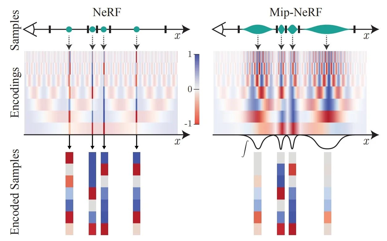
Results and Ablations
Quantitative performance The below table reports performance on the multiscale Blender dataset (credit: [29]), comparing Mip-NeRF to baseline NeRF and several improved NeRF variants. Mip-NeRF achieves the highest PSNR and SSIM across all scales (Full, 1/2, 1/4, 1/8 resolution), while reducing LPIPS—a perceptual dissimilarity metric—to the lowest values. The performance gap widens as the resolution decreases, demonstrating Mip-NeRF’s robustness to scale changes. Notably, removing IPE (w/o IPE) drops PSNR by up to \(6\,\mathrm {dB}\) at the lowest resolution, confirming its central role in anti-aliasing.
PSNR \(\uparrow \) | SSIM \(\uparrow \) | LPIPS \(\downarrow \) | Avg. \(\downarrow \) | Time (h) | #Params | ||||||||||
|---|---|---|---|---|---|---|---|---|---|---|---|---|---|---|---|
| FR | 1/2 | 1/4 | 1/8 | FR | 1/2 | 1/4 | 1/8 | FR | 1/2 | 1/4 | 1/8 | ||||
| NeRF (Jax Impl.) | 31.196 | 30.647 | 26.252 | 22.533 | 0.9498 | 0.9560 | 0.9299 | 0.8709 | 0.0546 | 0.0342 | 0.0428 | 0.0750 | 0.0288 | 3.05 | 1,191K |
| NeRF + Area Loss | 27.224 | 29.578 | 29.445 | 25.039 | 0.9113 | 0.9394 | 0.9524 | 0.9176 | 0.1041 | 0.0677 | 0.0406 | 0.0469 | 0.0305 | 3.03 | 1,191K |
| NeRF + Area, Centered Pix. | 29.893 | 32.118 | 33.399 | 29.463 | 0.9376 | 0.9590 | 0.9728 | 0.9620 | 0.0747 | 0.0405 | 0.0245 | 0.0398 | 0.0191 | 3.02 | 1,191K |
| NeRF + Area, Center, Misc. | 29.900 | 32.127 | 33.404 | 29.470 | 0.9378 | 0.9592 | 0.9730 | 0.9622 | 0.0743 | 0.0402 | 0.0243 | 0.0394 | 0.0190 | 2.94 | 1,191K |
| Mip-NeRF | 32.629 | 34.336 | 35.471 | 35.602 | 0.9579 | 0.9703 | 0.9786 | 0.9833 | 0.0469 | 0.0260 | 0.0168 | 0.0120 | 0.0114 | 2.84 | 612K |
| Mip-NeRF w/o Misc. | 32.610 | 34.333 | 35.497 | 35.638 | 0.9577 | 0.9703 | 0.9787 | 0.9834 | 0.0470 | 0.0259 | 0.0167 | 0.0120 | 0.0114 | 2.82 | 612K |
| Mip-NeRF w/o Single MLP | 32.401 | 34.131 | 35.462 | 35.967 | 0.9566 | 0.9693 | 0.9780 | 0.9834 | 0.0479 | 0.0268 | 0.0169 | 0.0116 | 0.0115 | 3.40 | 1,191K |
| Mip-NeRF w/o Area Loss | 33.059 | 34.280 | 33.866 | 30.714 | 0.9605 | 0.9704 | 0.9747 | 0.9679 | 0.0427 | 0.0256 | 0.0213 | 0.0308 | 0.0139 | 2.82 | 612K |
| Mip-NeRF w/o IPE | 29.876 | 32.160 | 33.679 | 29.647 | 0.9384 | 0.9602 | 0.9742 | 0.9633 | 0.0742 | 0.0393 | 0.0226 | 0.0378 | 0.0186 | 2.79 | 612K |
Qualitative performance The following figure shows visual comparisons on two Blender scenes across four scales. We crop a fixed region and display it as an image pyramid; the SSIM for each scale is shown in the lower-right, with the highest values (most successful SSIM results) highlighted in red. Mip-NeRF consistently outperforms NeRF and its improved variants both visually (fewer moiré patterns, crisper low-res textures) and quantitatively. The benefit is most pronounced at extreme downscales (1/8 res), where NeRF exhibits heavy aliasing but Mip-NeRF maintains smooth, faithful structure.
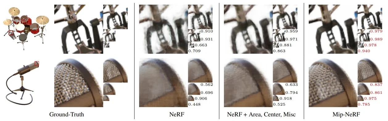
Ablation insights (following table 23.9)
- IPE is essential: Removing IPE reduces PSNR by up to \(6\,\mathrm {dB}\) at 1/8 resolution and greatly increases LPIPS, confirming it as the core mechanism for anti-aliasing.
- Moment-matching matters: Approximations that do not match the frustum’s true mean/variance (e.g., naive Gaussian) blur thin structures and lower both SSIM and PSNR.
- Area loss aids stability: Removing the area loss degrades performance at extreme scales, suggesting it complements IPE by regularizing footprint integration.
- Parameter efficiency: Mip-NeRF achieves superior results with roughly half the parameters of the baseline NeRF (612K vs 1.19M), aided by its single-scale-aware MLP.
Generalization to unseen scales In experiments with randomized camera zooms at test time, Mip-NeRF preserves detail and avoids aliasing even at scales never seen during training. This supports the mipmap analogy: each sample’s feature vector is already pre-filtered to match its footprint, so no extra post-processing is needed.
Limitations and Downsides
While Mip-NeRF mitigates scale aliasing, it inherits several constraints from the original NeRF:
- Bounded scene assumption: Optimized for forward-facing or spatially bounded scenes, making it ill-suited for large unbounded environments without further modification.
- View-dependent aliasing: IPE attenuates spatial high frequencies but does not pre-filter rapid view-dependent effects (e.g., specular highlights, reflections), which can still alias.
- Extra per-sample cost: Computing frustum moments and performing Gaussian integration introduce modest runtime overhead, although the reduced parameter count partly offsets this.
- Parameter sensitivity: Inaccurate cone-slope estimates or moment approximations can lead to over-blurring or residual aliasing.
These factors have motivated extensions that adapt IPE to broader settings, improve efficiency, or integrate it into hybrid scene representations.
Notable Works Building on Mip-NeRF
Mip-NeRF’s conical frustum integration and integrated positional encoding (IPE) have proven to be broadly reusable primitives. By explicitly encoding the spatial extent of each ray sample, these techniques offer a general anti-aliasing mechanism that can be slotted into diverse neural scene representations. As a result, subsequent works have adopted Mip-NeRF’s ideas to tackle new regimes such as unbounded scenes, high-speed rendering, and multi-modal supervision.
- Mip-NeRF 360 [28]: Extends Mip-NeRF to large, unbounded 360\(^\circ \) scenes via scene contraction, a distortion-based sampling loss, and multi-scale proposal networks. Retains the IPE formulation to prevent aliasing under extreme zoom or wide-FOV capture.
- Zip-NeRF [30]: Improves generalization to novel scenes by combining Mip-NeRF’s IPE with strong geometry priors and data-driven regularization. Achieves higher quality with fewer views and reduced overfitting.
- Tri-MipRF [247]: Integrates multi-resolution IPE into a tri-plane radiance field representation, yielding faster rendering while preserving Mip-NeRF’s anti-aliasing benefits.
- Gaussian Splatting with IPE (e.g., [299], follow-up variants): Adapts Mip-NeRF’s scale-aware encoding to initialize or filter point/ellipsoid attributes in real-time splatting pipelines, improving detail retention at varying scales.
Enrichment 23.10.7: NeuS: Neural Implicit Surfaces by Volume Rendering
Motivation
Surface reconstruction from multi-view images is a long-standing problem in computer vision. Classical multi-view stereo (MVS) pipelines such as COLMAP produce dense point clouds and polygon meshes, but often fail to recover fine details or handle challenging lighting and textureless regions. Neural scene representations, notably NeRF [442], have recently demonstrated photorealistic novel view synthesis, but NeRF’s volume rendering formulation inherently represents scenes as semi-transparent volumes rather than sharp, watertight surfaces. This leads to fuzzy geometry and small-scale surface artifacts, particularly when extracting explicit meshes.
An alternative is to represent scenes via a signed distance function (SDF), as in methods like IDR [753], which directly target surface rendering. SDF-based approaches tend to produce cleaner and more accurate surfaces, but prior work couples SDFs with classical surface rendering equations that do not model complex light transport along the ray. This makes them susceptible to catastrophic failures under occlusion: for example, IDR can produce visually plausible but geometrically incorrect reconstructions that “fill in” occluded spaces with spurious surfaces.
The following figure from the NeuS paper [688] illustrates this trade-off. In the bamboo planter example, IDR produces a clean-looking but topologically incorrect surface by filling the interior; NeRF better preserves the hollow geometry but introduces visible surface noise due to volumetric density smoothness. NeuS aims to combine the strengths of both: the sharp geometry of SDF-based surfaces and the photometric consistency of volumetric rendering.
To achieve this, NeuS reformulates the volume rendering weights so that they are derived directly from the SDF, enabling differentiable, unbiased surface localization while retaining the correct transmittance behavior of volumetric rendering. This addresses a key bias problem in naive SDF-to-density conversions (see the following figure), where the weight distribution shifts away from the true surface, leading to systematic depth errors. By aligning the rendering formulation with the signed distance geometry, NeuS bridges the gap between surface-based and volume-based neural reconstruction.
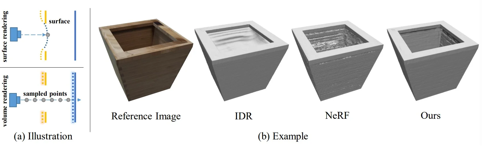
Method
Scene representation and rendering objective NeuS [688] directly learns an implicit Signed Distance Function (SDF) \( f_\theta : \mathbb {R}^3 \rightarrow \mathbb {R} \). For any point \(\mathbf {x} \in \mathbb {R}^3\), \(f_\theta (\mathbf {x})\) is the signed Euclidean distance to the closest point on the scene’s surface, with the zero level set \(\{\mathbf {x} \mid f_\theta (\mathbf {x}) = 0\}\) defining the surface itself: \[ f_\theta (\mathbf {x}) = \begin {cases} < 0, & \mathbf {x} \ \mbox{is inside the surface}, \\ = 0, & \mathbf {x} \ \mbox{is on the surface}, \\ > 0, & \mathbf {x} \ \mbox{is outside the surface}. \end {cases} \] By definition, this covers any number of disconnected or self-occluding surfaces — at each spatial location we only care about the distance to the nearest one, so a single continuous function \(f_\theta \) can represent multi-object scenes and thin structures.
Along a camera ray \(\mathbf {r}(t) = \mathbf {o} + t\,\mathbf {d}\), it is possible to have two depths \(t_0 < t_1\) such that \[ f_\theta (\mathbf {r}(t_0)) = f_\theta (\mathbf {r}(t_1)), \] even though these correspond to entirely different physical surfaces (e.g., a nearer front face and a farther back face with the same signed distance magnitude). For physically correct rendering, the nearer point \(\mathbf {r}(t_0)\) should contribute more to the pixel color than the farther one \(\mathbf {r}(t_1)\), since the latter is occluded by the former. NeuS therefore imposes the occlusion-aware requirement: if \(t_a < t_b\) and \(f_\theta (\mathbf {r}(t_a)) = f_\theta (\mathbf {r}(t_b))\), then \(w(t_a) > w(t_b)\), where \(w(t)\) is the per-sample weight along the ray.
The pixel color is modeled as a line integral of per-sample radiance contributions: \[ C(\mathbf {r}) \;=\; \int _{0}^{+\infty } w(t)\; c\!\big (\mathbf {r}(t),\mathbf {d}\big )\, dt, \] where \(c(\mathbf {r}(t),\mathbf {d})\) is the view-dependent color at position \(\mathbf {r}(t)\), and \(w(t)\) is a weight we will derive from the SDF following the paper’s Eqs. (2)–(13). Intuitively,
- \(w(t)\) must (i) peak exactly at the zero level set to avoid geometric bias.
- \(w(t)\) must respect occlusion so that nearer visible surfaces dominate the pixel color.
From SDF to volume rendering In the previous discussion we treated the signed distance function \(f_\theta \) as a given geometric primitive. In NeuS [688], this SDF is not precomputed — it is represented by a trainable multi-layer perceptron (MLP) that maps any 3D coordinate \(\mathbf {x}=(x,y,z)\) to its signed distance from the scene surface. The MLP typically uses positional encoding on \(\mathbf {x}\) to capture high-frequency detail, residual skip connections for stable optimization, and smooth activations such as Softplus to make the SDF differentiable everywhere. Training this network from multi-view images requires coupling the implicit geometry to a differentiable volume rendering model, so that image-space supervision can update the 3D SDF parameters.
The central design question is: given an SDF field \(f_\theta \), how should we convert it into per-ray weights \(w(t)\) for rendering, such that surfaces are accurately located and occlusion is respected? NeuS approaches this by interpreting the SDF along a ray as defining a probabilistic surface location.
Specifically, instead of learning a free-form volume density \(\sigma (t)\) as in the original NeRF, NeuS derives it directly from the signed distance function \(f_\theta \) so that the density field is geometrically tied to the zero-level set representing the surface. To do this, NeuS uses the logistic cumulative distribution function (CDF) and its derivative: \[ \Phi _s(x) = \frac {1}{1 + e^{-s x}}, \qquad \phi _s(x) = \Phi _s'(x) = \frac {s\,e^{-s x}}{\big (1+e^{-s x}\big )^2}, \] where \(s > 0\) controls sharpness (spread \(1/s\)) and is learned jointly with the SDF parameters.
Why the logistic family?
- The derivative \(\phi _s(x)\) is a smooth, symmetric, unimodal “bump” centered at \(x=0\), which makes it well-suited for concentrating density exactly at the surface (\(f_\theta (\mathbf {x}) = 0\)) while avoiding the discontinuities that would make optimization unstable.
- The CDF \(\Phi _s(x)\) transitions smoothly from 0 (far inside) to 1 (far outside) across the surface, providing a continuous and differentiable notion of “inside” vs. “outside” that plugs directly into the transmittance computation in volume rendering.
- Learning \(s\) allows the method to adapt the thickness of the high-density region during training: early on, a lower \(s\) produces a wider band of nonzero density around the surface, which increases the number of samples along a ray that contribute gradients and thus stabilizes learning. As training progresses, \(s\) increases, narrowing this band to approach the physical reality of an infinitely thin surface — effectively concentrating the density into a subpixel-scale layer for sharper geometry and cleaner renderings.
- In contrast, NeRF learns a free-form volume density \(\sigma (\mathbf {x})\) without explicitly enforcing a geometric zero-level surface. This can lead to inconsistencies between the geometry implied by the density field and the appearance in rendered images. NeuS’s SDF-driven density formulation ensures that the geometry and appearance are linked through the same underlying surface definition.
When applied along a ray \(\mathbf {r}(t)\), \(\phi _s(f_\theta (\mathbf {r}(t)))\) acts as a surface-likelihood profile: it peaks where the ray intersects the surface and decays smoothly away from it. To produce physically correct renderings, this profile must be combined with an occlusion-aware transmittance term so that nearer intersections dominate over farther ones, and it must be constructed to be unbiased — i.e., its maximum should occur exactly at \(f_\theta (\mathbf {r}(t)) = 0\). The derivation of such an unbiased, occlusion-aware weight \(w(t)\) from \(\Phi _s\) and \(\phi _s\) is the focus of the next section.
Naïve SDF\(\to \)density conversion and its bias A straightforward NeRF-style mapping would define \[ w_{\mbox{naive}}(t) = T(t)\,\sigma (t), \quad T(t)=\exp \!\Big (-\int _{0}^{t}\sigma (u)\,du\Big ), \quad \sigma (t)=\phi _s\big (f_\theta (\mathbf {r}(t))\big ), \] where \(T(t)\) is the accumulated transmittance and \(\sigma (t)\) is the “density” derived from the SDF. This form is naturally occlusion-aware due to \(T(t)\), but the product \(T(t)\,\sigma (t)\) tends to peak before the actual surface intersection \(f_\theta (\mathbf {r}(t^*))=0\), introducing a geometric bias. Intuitively, as \(\sigma (t)\) rises approaching the surface, \(T(t)\) is already decaying, shifting the peak forward along the ray (The following figure shows exactly that).
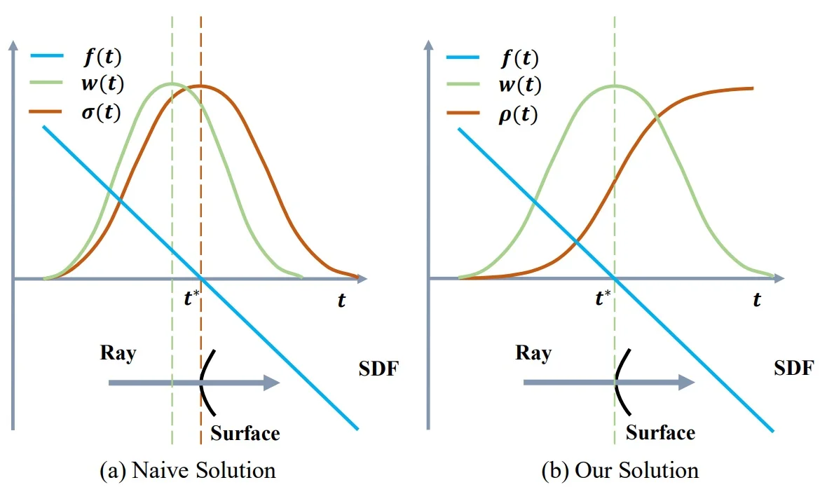
A direct unbiased weighting that fails occlusion A seemingly natural way to obtain an unbiased surface-localization weight from the SDF is to normalize the S-density along the ray: \[ w_{\mbox{dir}}(t) = \frac {\phi _s\big (f(\mathbf {r}(t))\big )}{\int _{0}^{+\infty } \phi _s\big (f(\mathbf {r}(u))\big ) \, du}. \] Here, the numerator \(\phi _s(f(\mathbf {r}(t)))\) is maximal exactly when \(f(\mathbf {r}(t))=0\), i.e., at the true surface intersection, because \(\phi _s\) is a smooth, unimodal density centered at zero. This guarantees that \(w_{\mbox{dir}}(t)\) peaks at the correct location—hence “unbiased.”
However, this construction ignores depth ordering and thus fails to model occlusion. If a ray encounters multiple surfaces, the SDF \(f(\mathbf {r}(t))\) will cross zero at each intersection, producing multiple peaks in \(\phi _s(f(\mathbf {r}(t)))\). Since \(w_{\mbox{dir}}(t)\) is obtained by global normalization of these peaks, the contributions from all intersections are rescaled to sum to one and are all blended into the final color. Crucially, no mechanism here suppresses the influence of farther intersections once a nearer one has been reached—violating the physical visibility constraint that closer surfaces should occlude those behind them.
This limitation motivates the NeuS formulation, which retains the precise, unbiased surface localization of \(w_{\mbox{dir}}\) while introducing an occlusion-aware transmittance term so that nearer surfaces dominate the final rendered pixel.
Derivation of the NeuS Weight Function for the Single-Plane Case
We begin with the simplest setting: a single infinite plane intersected by one camera ray.
Step 1: Geometric Setup Let the ray be parameterized as \begin {equation} \mathbf {p}(t) = \mathbf {o} + t\,\mathbf {v}, \quad t \geq 0, \end {equation} where \(\mathbf {o} \in \mathbb {R}^3\) is the camera origin, \(\mathbf {v} \in \mathbb {S}^2\) is a unit direction vector, and \(t\) denotes depth along the ray. Let \(t^*\) be the depth where the signed distance function (SDF) vanishes: \begin {equation} f(\mathbf {p}(t^*)) = 0. \end {equation}
Step 2: Normal and Incidence Angle Let \(\mathbf {n}\) be the unit outward normal of the plane. The incidence angle \(\theta \) is defined by \begin {equation} \cos \theta = \mathbf {v} \cdot \mathbf {n}. \end {equation} A perpendicular hit yields \(|\cos \theta | = 1\), while grazing incidence has \(|\cos \theta | \approx 0\).
Step 3: SDF properties (geometry and intuition) A true signed distance function (SDF) \(f:\mathbb {R}^3 \to \mathbb {R}\) satisfies, almost everywhere, \begin {equation} \nabla f(\mathbf {x}) = \mathbf {n}(\mathbf {x}), \qquad \|\nabla f(\mathbf {x})\|_2 = 1, \end {equation} where \(\mathbf {n}(\mathbf {x})\) is the outward unit normal to the surface at the closest point \(\pi (\mathbf {x})\).
- Gradient equals the normal. Consider moving \(\mathbf {x}\) in a tangent direction \(\mathbf {t}\) at \(\pi (\mathbf {x})\). The closest-point distance does not change to first order: \[ \frac {\partial f}{\partial t}(\mathbf {x}) = 0 \quad \mbox{for all tangents $\mathbf {t}$ at $\pi (\mathbf {x})$}. \] In contrast, moving along the normal \(\mathbf {n}(\pi (\mathbf {x}))\) increases the signed distance at the maximal possible rate: \[ \frac {\partial f}{\partial n}(\mathbf {x}) = 1. \] The gradient \(\nabla f(\mathbf {x})\) is the vector collecting all directional derivatives. The fact that tangent derivatives are zero and the normal derivative is exactly \(1\) implies \[ \nabla f(\mathbf {x}) = \mathbf {n}(\pi (\mathbf {x})), \] i.e., the gradient is not only parallel to the surface normal but identical to it.
- Unit slope. By the definition of distance, taking a small step \(\delta \) along the outward normal \[ \mathbf {x}_\delta = \pi (\mathbf {x}) + \delta \,\mathbf {n}(\pi (\mathbf {x})) \] changes the signed distance by exactly \(\delta \): \[ f(\mathbf {x}_\delta ) = f(\pi (\mathbf {x})) + \delta = \delta . \] Therefore, \[ \frac {d}{d\delta } f(\mathbf {x}_\delta )\Big |_{\delta =0} = 1 \] and since this is the derivative in the gradient’s direction, we must have \(\|\nabla f(\mathbf {x})\|_2 = 1\).
Equivalently, a perfect SDF solves the Eikonal equation \(\|\nabla f\|_2 = 1\) with \(f = 0\) on the surface, except on the medial axis where the nearest point is not unique. In learned SDFs, this property is encouraged by the Eikonal regularizer \((\|\nabla f\|_2 - 1)^2\), which ensures correct metric scaling and underpins the angle-based derivations in Step 4.
Step 4: SDF Evolution Along the Ray By the chain rule, \begin {equation} \frac {df}{dt} = \nabla f(\mathbf {p}(t)) \cdot \frac {d\mathbf {p}}{dt} = \mathbf {n} \cdot \mathbf {v} = \cos \theta . \end {equation} With the convention \(f > 0\) outside the surface, \(f < 0\) inside, an entering ray satisfies \(\cos \theta < 0\): \begin {equation} \frac {df}{dt} = -\,|\cos \theta |. \end {equation}
Step 5: Local linearization near the surface Let \(t^*\) be the depth at which the ray \(\mathbf {p}(t) = \mathbf {o} + t\,\mathbf {v}\) intersects the surface, i.e., \(f(\mathbf {p}(t^*)) = 0\). From Step 4 we know that \[ \frac {df}{dt} = \nabla f \cdot \frac {d\mathbf {p}}{dt} = \mathbf {n}(\mathbf {p}(t)) \cdot \mathbf {v}. \] At \(t = t^*\), the gradient equals the outward unit normal, \(\mathbf {n}(\mathbf {p}(t^*))\), so \[ \frac {df}{dt}\Big |_{t^*} = \mathbf {n}(\mathbf {p}(t^*)) \cdot \mathbf {v} = -\,|\cos \theta |, \] where \(\theta \) is the incidence angle between the ray and the normal; the minus sign follows from the convention \(f>0\) outside the surface.
First-order approximation: Under the tangent-plane assumption near \(\mathbf {p}(t^*)\), the unit normal \(\mathbf {n}\) is constant in this neighborhood. From Step 4, along the ray \(\mathbf {p}(t)\) we have \[ \frac {df}{dt} = \mathbf {n} \cdot \mathbf {v} = -\,|\cos \theta | \quad \mbox{(constant)}. \] This is an ordinary differential equation with constant right-hand side. Integrating both sides with respect to \(t\) from \(t^*\) to \(t\) gives \[ f(\mathbf {p}(t)) - f(\mathbf {p}(t^*)) = -\,|\cos \theta |\,(t - t^*). \] Since \(f(\mathbf {p}(t^*)) = 0\) (the ray is on the surface at \(t^*\)), we obtain \begin {equation} f(\mathbf {p}(t)) \;=\; -\,|\cos \theta |\,\big (t - t^*\big ). \end {equation}
Interpretation:
- \(t < t^* \ \Rightarrow \ f > 0\): the sample lies outside the surface.
- \(t = t^* \ \Rightarrow \ f = 0\): the sample lies on the surface.
- \(t > t^* \ \Rightarrow \ f < 0\): the sample lies inside the surface.
The slope magnitude \(|\cos \theta |\) measures how quickly the signed distance changes along the ray: grazing rays (\(\theta \) near \(90^\circ \)) change \(f\) slowly, while near-normal rays (\(\theta \) near \(0^\circ \)) change it rapidly. This angular factor is exactly what Step 6 will remove to construct a per-depth weight that is unbiased with respect to the ray–surface angle.
Step 6: Direct unbiased weight construction Let \(\Phi _s\) be the logistic CDF with sharpness \(s\), and \(\phi _s = \Phi _s'\) its PDF (the S-density). A naive choice, \begin {equation} w(t)=\phi _s\big (f(\mathbf {p}(t))\big ), \end {equation} produces a bell-shaped bump centered at the true hit depth \(t^*\), but its area in \(t\)-space scales like \(1/|\cos \theta |\). Intuition: along the ray, \(f(\mathbf {p}(t))\) changes at rate \(\big |\tfrac {df}{dt}\big | = |\cos \theta |\) (Step 4). Grazing rays (\(|\cos \theta |\!\ll \!1\)) sweep through the same range of SDF values more slowly, stretching the bump in depth; hence, more total weight accumulates in free space before the hit than for a head-on ray. This angle-dependent “mass inflation” is undesirable: it skews how much a single opaque surface contributes depending on view angle and can over-emphasize pre-surface samples.
Normalization (single-plane model). To remove this geometric inflation, we normalize by the total area along the ray: \begin {equation} w_{\mathrm {dir}}(t) \;=\; \frac {\phi _s\big (f(\mathbf {p}(t))\big )} {\displaystyle \int _{0}^{+\infty }\phi _s\big (f(\mathbf {p}(u))\big )\,du}. \end {equation} Under the local planar model of Step 5, \(f(\mathbf {p}(u))=-\,|\cos \theta |\,(u-t^*)\) and \(\tfrac {df}{du}=-\,|\cos \theta |\). With the change of variables \(x=f(\mathbf {p}(u))\) (so \(du=-\,dx/|\cos \theta |\)) we obtain \begin {equation} \int _{0}^{+\infty }\phi _s\big (f(\mathbf {p}(u))\big )\,du \;=\; \frac {1}{|\cos \theta |} \int _{x_{\min }}^{x_{\max }} \phi _s(x)\,dx, \end {equation} where \(x_{\min } = -\,|\cos \theta |\,t^*\) and \(x_{\max } \to +\infty \). In the idealized infinite-depth limit \(t^*\to +\infty \), \begin {equation} \lim _{t^*\to +\infty } \int _{0}^{+\infty }\phi _s\big (f(\mathbf {p}(u))\big )\,du \;=\; \frac {1}{|\cos \theta |} \int _{-\infty }^{+\infty }\phi _s(x)\,dx \;=\; \frac {1}{|\cos \theta |}. \end {equation} Hence, in this limit, the direct single-plane weight becomes \begin {equation} \boxed {\,w(t) \;=\; |\cos \theta |\,\phi _s\!\big (f(\mathbf {p}(t))\big ).\,} \end {equation} For finite \(t^*\), this expression is an accurate approximation whenever the support of \(\phi _s\) lies well inside the integration domain.
Why normalization removes the bias (formal & intuitive). Let \(k := |\cos \theta |\) and \(f(\mathbf {p}(t)) = -\,k\,(t-t^*)\) near \(t^*\).
-
(i) Unit mass, angle-invariant. \begin {align} \int _{0}^{+\infty } w(t)\,dt \;=\; k \!\int _{0}^{+\infty } \phi _s\!\big (f(\mathbf {p}(t))\big )\,dt \overset {x=f}{=} k \!\int _{x=f(\mathbf {p}(+\infty ))}^{x=f(\mathbf {p}(0))} \phi _s(x)\,\frac {-dx}{k} \;\approx \; \int _{-\infty }^{+\infty } \phi _s(x)\,dx \;=\; 1, \end {align}
where the approximation becomes exact as \(t^*\!\to \!+\infty \). Intuition: the bump widens by \(1/k\) for grazing rays, and the prefactor \(k\) exactly scales its height so that the total area remains \(1\).
- (ii) No pre-surface overweighting. Under the same change of variables, \(t<t^*\!\iff \!x>0\) and \(t>t^*\!\iff \!x<0\). Since \(\phi _s\) is symmetric, \begin {equation} \int _{t<t^*} w(t)\,dt \;=\; \int _{x>0} \phi _s(x)\,dx \;=\; \tfrac {1}{2} \;=\; \int _{x<0} \phi _s(x)\,dx \;=\; \int _{t>t^*} w(t)\,dt, \end {equation} again exact in the \(t^*\!\to \!+\infty \) limit (or whenever both tails of \(\phi _s\) are contained in the integration domain). Thus the fraction of weight allocated before the hit is fixed at \(1/2\)—grazing rays do not gain extra early mass. Moreover, the distribution of \((t-t^*)\) under \(w\) is symmetric, so \(\mathbb {E}_w[t]=t^*\): there is no forward shift of the “center of mass.”
- (iii) Peak at the surface (no forward drift). Because \(\phi _s\) is unimodal with maximum at \(x=0\), \(w(t)\propto \phi _s(f(\mathbf {p}(t)))\) attains its maximum at \(f=0\), i.e., exactly at \(t=t^*\). Hence \(w(t^*) > w(t)\) for all \(t \neq t^*\).
Step 7: Derivative-of-CDF Identity From Step 4 we know that along the ray \[ \frac {df}{dt} \;=\; \mathbf {n}\!\cdot \!\mathbf {v} \;=\; -\,|\cos \theta |, \] for an entering ray. Applying the chain rule to the cumulative distribution \(\Phi _s(f(\mathbf {p}(t)))\) gives \begin {equation} \frac {d}{dt}\,\Phi _s\!\big (f(\mathbf {p}(t))\big ) \;=\; \phi _s\!\big (f(\mathbf {p}(t))\big )\,\frac {df}{dt} \;=\; -\,|\cos \theta |\,\phi _s\!\big (f(\mathbf {p}(t))\big ). \end {equation} Thus the NeuS weight may be expressed as \begin {equation} \boxed {\,w(t) \;=\; |\cos \theta |\,\phi _s(f(\mathbf {p}(t))) \;=\; -\,\tfrac {d}{dt}\,\Phi _s(f(\mathbf {p}(t))).\,} \end {equation}
Step 8: Interpretation as Soft Visibility The function \(\Phi _s(f(\mathbf {p}(t)))\) acts as a soft visibility function:
- Outside the surface (\(f>0\)), \(\Phi _s \approx 1\), meaning the ray is fully visible.
- Deep inside (\(f<0\)), \(\Phi _s \approx 0\), meaning the ray has been completely occluded.
- Near the zero-level set, \(\Phi _s\) smoothly transitions between these values.
The weight \(w(t)\) is precisely the negative slope of this transition along depth, concentrating probability where the ray crosses the soft band around the surface.
Step 9: Embedding into Volume Rendering Classical volume rendering defines \[ w(t) \;=\; T(t)\,\rho (t), \qquad T'(t) = -\,\rho (t)\,T(t). \] Identifying \begin {equation} T(t) \;=\; \Phi _s(f(\mathbf {p}(t))), \end {equation} we obtain \begin {equation} \rho (t) \;=\; \frac {w(t)}{T(t)} = \frac {-\tfrac {d}{dt}\,\Phi _s(f(\mathbf {p}(t)))}{\Phi _s(f(\mathbf {p}(t)))}. \end {equation} Hence the NeuS construction ensures \[ w(t) \;=\; T(t)\rho (t), \] so the derivative-of-CDF weight integrates seamlessly into the unbiased volume rendering framework.
Multi-Surface Generalization
Up to now we have assumed a single, locally planar zero-level set with a consistent orientation (entering side only). In realistic 3D scenes, however, a ray may intersect multiple surfaces (e.g., front and back faces of an object), or may exit a surface region where the signed distance field increases in the viewing direction (\(df/dt > 0\)). This introduces two problems:
- 1.
- The raw expression \[ \rho (t) \;=\; -\,\frac {d}{dt}\,\log \Phi _s(f(\mathbf {p}(t))) \] can become negative when \(df/dt > 0\), leading to unphysical “negative density”.
- 2.
- Without correction, the transmittance \(T(t) = \exp \!\left (-\int _0^t \rho (u)\,du\right )\) could become increasing, which contradicts the physical principle that visibility along a ray must monotonically decrease.
Enforcing Physical Validity NeuS resolves these issues by clipping the density: \begin {equation} \rho (t) \;=\; \max \!\left ( -\,\frac {\tfrac {d}{dt}\,\Phi _s(f(\mathbf {p}(t)))}{\Phi _s(f(\mathbf {p}(t)))}, \, 0 \right ). \end {equation} This guarantees that \(\rho (t) \geq 0\), so that transmittance is non-increasing and weights \(w(t) = T(t)\rho (t)\) remain physically consistent.
Intuition One way to view this is to imagine the ray entering and leaving a “soft surface band”. On the entering side (\(df/dt < 0\)), the visibility drops and the derivative contributes positive density. On the exiting side (\(df/dt > 0\)), visibility recovers; the raw derivative would suggest negative density, but NeuS suppresses this contribution to avoid creating “ghost” surfaces with negative opacity. In effect, NeuS only accumulates mass where surfaces occlude the ray, never where they re-open.
Weights Construction Summary In the single-surface case, the NeuS weight \[ w(t) = |\cos \theta | \,\phi _s(f(\mathbf {p}(t))) \] is unbiased: it integrates to one, splits symmetrically around the true intersection, and peaks exactly at the surface crossing. The clipping-based generalization ensures that this property extends to arbitrary, multi-surface geometry, embedding the construction into the physically consistent volume rendering framework.
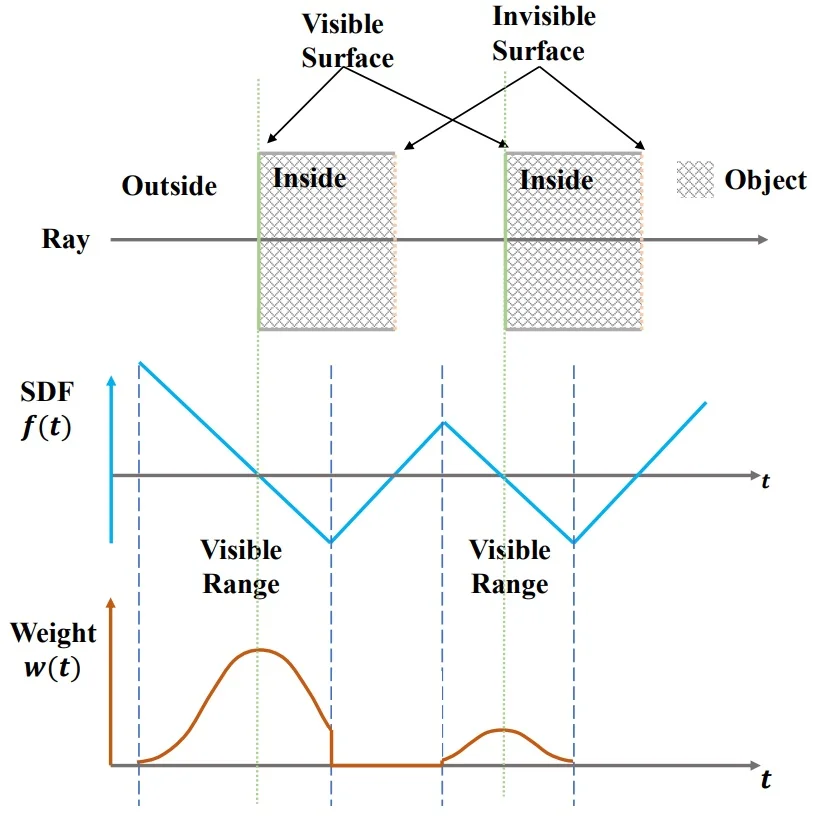
Discretization To obtain discrete counterparts of the opacity and weight functions, the authors used the same approximation scheme as used in NeRF [442]. Specifically, they sample \(n\) points along a ray, \[ p_i = \mathbf {o} + t_i \mathbf {v}, \quad i=1,\dots ,n, \quad t_i < t_{i+1}, \] and approximate the pixel color of the ray as \begin {equation} \hat {C} = \sum _{i=1}^{n} T_i \,\alpha _i \, c_i, \end {equation} where \(T_i\) denotes the discrete accumulated transmittance, defined by \[ T_i = \prod _{j=1}^{i-1} (1 - \alpha _j), \] and \(\alpha _i\) represents the discrete opacity given by \begin {equation} \alpha _i = 1 - \exp \!\left ( - \int _{t_i}^{t_{i+1}} \rho (t) \, dt \right ). \end {equation} Using the NeuS definition of the \(s\)-density \(\rho (t)\), this integral can be shown to yield \begin {equation} \alpha _i = \max \!\left ( \frac {\Phi _s(f(p_i)) - \Phi _s(f(p_{i+1}))}{\Phi _s(f(p_i))}, \, 0 \right ), \end {equation}
where \(\Phi _s\) is the cumulative distribution induced by the sigmoid with sharpness parameter \(s\). The term \(c_i\) is obtained by evaluating the radiance branch of the MLP at the point \(\mathbf {x}_i\) and viewing direction \(\mathbf {d}\), giving \(c_i = c(\mathbf {x}_i,\mathbf {d})\). Importantly, NeuS does not eliminate the MLP; rather, it changes its parameterization. Instead of predicting a free density value \(\sigma (\mathbf {x})\) as in NeRF, the network outputs a signed distance value \(f_\theta (\mathbf {x})\). This is then converted into densities through the sigmoid-based cumulative distribution \(\Phi _s(f_\theta (\mathbf {x}))\), from which the discrete opacities \(\alpha _i\) are derived.
The max operator ensures non-negativity by clipping spurious increases of \(\Phi _s\) across bins. Thus the discretization remains faithful to the continuous NeuS rendering equation.
Compared to NeRF, the forward cost is essentially identical—both require evaluating an MLP for each sample. The key difference lies in representation: NeRF directly predicts densities, while NeuS predicts an SDF and enforces surface-consistency through its transformation. This change does not accelerate rendering, but it yields sharper, geometrically consistent surfaces and avoids the “fuzzy-shell” artifacts common to NeRF.
Training NeuS is trained without any ground-truth 3D supervision. Instead, it relies on standard 2D image supervision: observed pixel colors and, if available, binary foreground masks. The goal is to optimize the signed distance function \( f_\theta \) and color head so that the rendered radiance field explains all training views consistently.
Pixel sampling. At each iteration, a batch of \(m\) image pixels is sampled. For every pixel we collect its color, optional binary mask, and corresponding camera ray in world space: \[ P = \{ C_k, \, M_k, \, \mathbf {o}_k, \, \mathbf {v}_k \}_{k=1}^m, \] where \( C_k \in \mathbb {R}^3 \) is the observed RGB value, \( M_k \in \{0,1\} \) is the foreground/background indicator, \(\mathbf {o}_k\) is the camera origin, and \(\mathbf {v}_k\) the unit ray direction.
Overall objective. For each ray, \(n\) points are sampled and rendered through the NeuS volume rendering equation, producing predicted colors \(\hat {C}_k\) and occupancies \(\hat {O}_k\). The total training loss is \begin {equation} \mathcal {L} = \mathcal {L}_{\mbox{color}} + \lambda \, \mathcal {L}_{\mbox{reg}} + \beta \, \mathcal {L}_{\mbox{mask}}, \end {equation} where each term enforces a different supervision signal.
Color reconstruction. The primary signal is per-pixel color matching: \begin {equation} \mathcal {L}_{\mbox{color}} = \frac {1}{m} \sum _{k=1}^m \mathcal {R}(\hat {C}_k, C_k), \end {equation} where \(\mathcal {R}\) is an \(\ell _1\) loss, chosen for robustness to outliers. This term encourages the rendered radiance field to reproduce the ground-truth images.
Eikonal regularization. To ensure that \(f_\theta \) behaves as a valid signed distance function, NeuS adds an Eikonal loss [195]: \begin {equation} \mathcal {L}_{\mbox{reg}} = \frac {1}{nm} \sum _{k,i} \bigl (\|\nabla f(\hat {p}_{k,i})\|_2 - 1\bigr )^2, \end {equation} forcing the gradient norm to remain close to 1 almost everywhere.
Mask supervision. When binary foreground masks are available, NeuS includes an additional constraint on ray occupancy: \begin {equation} \mathcal {L}_{\mbox{mask}} = \mbox{BCE}(M_k, \hat {O}_k), \qquad \hat {O}_k = \sum _{i=1}^n T_{k,i}\alpha _{k,i}, \end {equation} where \(\hat {O}_k \in [0,1]\) is the predicted probability that ray \(k\) intersects the object. If \(M_k=0\) (background pixel), the network is penalized for predicting any opacity along that ray. If \(M_k=1\) (foreground), the network must explain the pixel with some nonzero occupancy. This mask loss thus provides strong geometric supervision in cases where silhouettes are known.
Hierarchical sampling. The hierarchical sampling strategy in NeuS is designed to efficiently localize the surface by focusing computation on regions where the signed distance field (SDF) indicates high surface likelihood. Importantly, NeuS achieves this with a single MLP, unlike NeRF which maintains separate coarse and fine networks.
- Stage 1: Uniform sampling with fixed sharpness. Each ray is first discretized into \(n_0\) uniformly spaced points (e.g., 64). For these coarse samples, NeuS evaluates the S-density function \[ \phi _{s}(f(x)) = \Phi _s(-f(x)) \cdot \left | \frac {\partial f}{\partial x} \right | \] using a fixed sharpness parameter \( s \). This fixed \( s \) is not learned but annealed over iterations (e.g., \( s = 32 \cdot 2^i \) in iteration \(i\)) so that the sampling distribution becomes progressively more peaked near potential surface regions. The goal is to obtain a broad but informative estimate of where surfaces may lie.
- Stage 2: Importance sampling with learned sharpness. Based on the coarse distribution, NeuS resamples additional \(n_1\) points (e.g., 4 iterations of 16 points each). For these fine samples, the probability density is computed with the learned sharpness parameter \(s\), which is optimized during training. This adaptive \(s\) sharpens over time, concentrating samples more tightly around the true surface as the SDF becomes well-defined.
Thus, NeuS does not use two separate networks but instead uses two different regimes of the same S-density function: one with fixed, annealed sharpness for exploration, and one with learned sharpness for exploitation. This hierarchical approach balances efficiency with precision: the fixed \(s\) ensures coverage so that surfaces are not missed, while the learned \(s\) allows the model to progressively refine and localize surfaces with high fidelity.
Compared to NeRF, where hierarchical sampling requires evaluating two full MLPs (a coarse and a fine model), NeuS is more efficient: only a single MLP is optimized and queried, with different sampling distributions guiding where along the ray the network is evaluated. Moreover, since NeuS is SDF-based, the learned sharpness naturally drives samples toward the zero level set, achieving more accurate and unbiased surface reconstruction than NeRF’s density-based formulation.
Training stabilization via geometry initialization Directly training an SDF-based radiance field from random initialization often leads to vanishing gradients, since no ray finds a valid surface early in optimization. To mitigate this, NeuS biases the final layer of the SDF network such that its zero-level set initially approximates a coarse sphere around the scene. This “geometry initialization” ensures that rays intersect meaningful surfaces at the start of training, stabilizing the optimization process. As learning progresses, the initialized surface quickly deforms to match the actual scene geometry.
Experiments and Ablations
Experimental setup NeuS is evaluated on the DTU dataset, which provides multi-view images with ground-truth geometry. Reconstructions are reported both with and without mask supervision. Mask supervision means that a foreground mask of the object is available during training, ensuring that background pixels do not bias the reconstruction. Without mask supervision, the method must disentangle object and background purely from image observations.
Quantitative results The following table reports Chamfer distance (lower is better) across multiple DTU scans, comparing NeuS to prior implicit reconstruction methods (IDR [753], UNISURF [469]) and to volumetric rendering baselines (NeRF [442]) and COLMAP [571]. NeuS consistently achieves the lowest mean error (0.84), significantly outperforming both NeRF and UNISURF.
| ScanID | IDR | NeRF | NeuS | COLMAP | NeRF (w/o mask) | UNISURF | NeuS (w/o mask) |
| 24 | 1.63 | 1.83 | 0.83 | 0.81 | 1.90 | 1.32 | 1.00 |
| 37 | 1.87 | 2.39 | 0.98 | 2.05 | 1.60 | 1.36 | 1.37 |
| 40 | 0.63 | 1.79 | 0.56 | 0.73 | 1.85 | 1.72 | 0.93 |
| 55 | 0.48 | 0.66 | 0.37 | 1.22 | 0.58 | 0.44 | 0.43 |
| 63 | 1.04 | 1.79 | 1.13 | 1.79 | 2.28 | 1.35 | 1.10 |
| 65 | 0.79 | 1.44 | 0.59 | 1.58 | 1.27 | 0.79 | 0.65 |
| 69 | 0.77 | 1.50 | 0.60 | 1.02 | 1.47 | 0.80 | 0.57 |
| 83 | 1.33 | 1.20 | 1.45 | 3.05 | 1.67 | 1.49 | 1.48 |
| 97 | 1.16 | 1.96 | 0.95 | 1.40 | 2.05 | 1.37 | 1.09 |
| 105 | 0.76 | 1.27 | 0.78 | 2.05 | 1.07 | 0.89 | 0.83 |
| 106 | 0.67 | 1.44 | 0.52 | 1.00 | 0.88 | 0.59 | 0.52 |
| 110 | 0.90 | 2.61 | 1.43 | 1.32 | 2.53 | 1.47 | 1.20 |
| 114 | 0.42 | 1.04 | 0.36 | 0.49 | 1.06 | 0.46 | 0.35 |
| 118 | 0.51 | 1.13 | 0.45 | 0.78 | 1.15 | 0.59 | 0.49 |
| 122 | 0.53 | 0.99 | 0.45 | 1.17 | 0.96 | 0.62 | 0.54 |
| Mean | 0.90 | 1.54 | 0.77 | 1.36 | 1.49 | 1.02 | 0.84 |
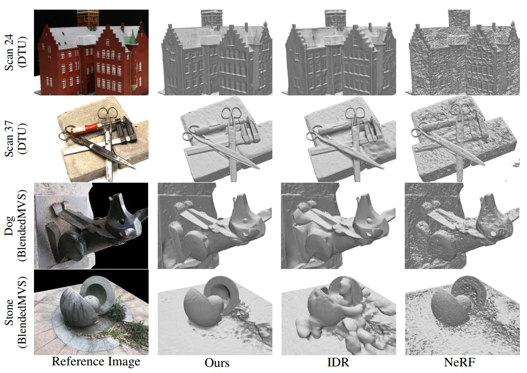
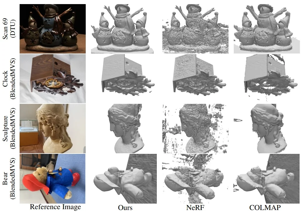
Ablation studies The contribution of each component in NeuS is verified via ablation. The following table reports Chamfer distance and mean absolute error (MAE) between ground-truth and predicted SDF values. The results highlight the necessity of all components: naive volume rendering (a) and direct SDF supervision (b) fail catastrophically; removing the Eikonal regularization (c) or geometry initialization (d) significantly degrades performance; only the full model (e) achieves low reconstruction error.
| Variant | Chamfer Distance | MAE |
| (a) Naive Solution | 1.49 | 1.75 |
| (b) Direct Solution | 4.45 | 44.34 |
| (c) w/o Eikonal | 0.64 | 88.94 |
| (d) w/o Geo-Init. | 0.62 | 6.19 |
| (e) Full Model | 0.59 | 0.93 |
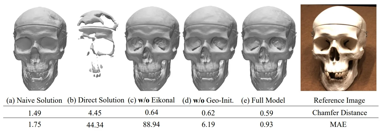
While NeuS delivers high-quality surface reconstructions via its signed distance field (SDF)–based volume rendering, it has notable limitations:
- Computational cost: The reliance on per-sample MLP evaluations and SDF-to-density conversion makes training and inference slower compared to standard NeRF pipelines.
- Mask dependency: Although NeuS works without mask supervision, accurate foreground masks significantly boost reconstruction fidelity; without them, detail in thin or complex structures can suffer.
- Topology challenges: Representing highly intricate or open surfaces remains a challenge for closed-surface SDF models.
Previous works.
- IDR [753]: Introduced differentiable rendering of implicit surfaces using signed distance functions (SDFs), supervising geometry through surface normals and photometric consistency. While conceptually elegant, IDR struggled with complex or open-topology scenes (e.g., buckets or vases), where normal-based rendering did not provide stable gradients. NeuS builds directly on IDR’s use of SDFs but resolves its instability by adopting a volume rendering formulation, yielding more consistent optimization signals and sharper reconstructions.
Concurrent works.
- VolSDF [754]: Proposed mapping SDF values to densities via a Laplace cumulative distribution function (CDF), enabling smoother and more stable volume rendering than IDR. However, VolSDF used a fixed sharpness parameter, which limited its ability to adapt across varying surface scales. NeuS improved on this by introducing a learnable sharpness, allowing adaptive localization of surfaces and producing significantly crisper reconstructions, especially in fine-detail regions.
- UNISURF [469]: Presented a unified framework bridging NeRF and implicit surface rendering. Unlike NeuS, UNISURF relied more heavily on external mask supervision, which limited its robustness in unconstrained scenarios. Both works shared the motivation of reconciling surface-based and volumetric representations, but NeuS advanced the field by learning the SDF-to-density mapping directly, reducing reliance on explicit segmentation cues.
Later works.
- HF-NeuS [704]: Decomposed the SDF into base and residual frequency components, enabling reconstruction of thin structures and high-frequency detail (e.g., sharp edges or wires). While improving fidelity compared to NeuS, it retained the same runtime bottlenecks since both relied on per-point MLP evaluation.
- PET-NeuS [705]: Replaced dense per-point MLP queries with tri-plane encodings, where features were stored in structured 2D planes and interpolated during rendering. This design improved efficiency and detail, addressing NeuS’s computational cost while preserving its SDF-based accuracy.
- NeUDF [385]: Generalized NeuS-style rendering to unsigned distance functions (UDFs), removing the assumption of closed surfaces inherent to SDFs. This allowed robust reconstructions of open and thin structures (e.g., curtains, leaves, or perforated objects) that NeuS struggled with, thus broadening applicability to more complex real-world geometries.
- KiloNeuS [148]: Partitioned the scene into thousands of small MLP “experts,” drastically reducing training and inference time. Compared to NeuS, which required hours of optimization, KiloNeuS achieved near real-time performance while maintaining competitive quality, making SDF-based rendering far more practical.
- NeuS2 [703]: Extended NeuS with hash-grid encodings and optimized CUDA kernels, reducing training from hours to minutes per scene. Crucially, NeuS2 also incorporated support for dynamic scenes, handling time-varying geometry and appearance—a limitation in the original NeuS. This positioned NeuS2 as a scalable and general successor.
- GSDF [767]: Combined NeuS-style SDF geometry with Gaussian Splatting for appearance modeling. The motivation was that SDFs excel at representing surfaces but are inefficient for view-dependent appearance, while Gaussians offer fast rasterization and smooth view interpolation. By splitting geometry (SDF) and appearance (Gaussians), GSDF improved both quality and rendering efficiency compared to pure NeuS.
Enrichment 23.10.8: Point-NeRF: Point-based Neural Radiance Fields
Point-NeRF [736] introduces a point-based neural radiance field representation that combines the strengths of explicit point clouds and implicit volumetric rendering. Unlike NeRF [442], which fits a global MLP per scene, Point-NeRF leverages neural point clouds that encode local geometry and appearance features, enabling efficient feed-forward initialization and rapid per-scene optimization. This summary details the motivation, method, architecture, experiments, limitations, and follow-up work.
Motivation
Classical NeRF methods achieve impressive view synthesis results but suffer from inefficiency: each scene requires hours or days of optimization, and significant computation is wasted sampling empty space. Point clouds, by contrast, provide explicit geometric priors but often suffer from holes, noise, or sparsity when reconstructed using MVS or SfM pipelines (e.g., COLMAP [571]).
Point-NeRF addresses both challenges by:
- Using neural points distributed near surfaces to avoid sampling empty space.
- Enabling direct feed-forward initialization of neural radiance fields via deep MVS prediction.
- Employing point pruning and growing to repair sparse or noisy point clouds.
This hybrid approach leads to reconstructions that surpass NeRF in quality and efficiency, converging in tens of minutes up to a several hours instead of days.
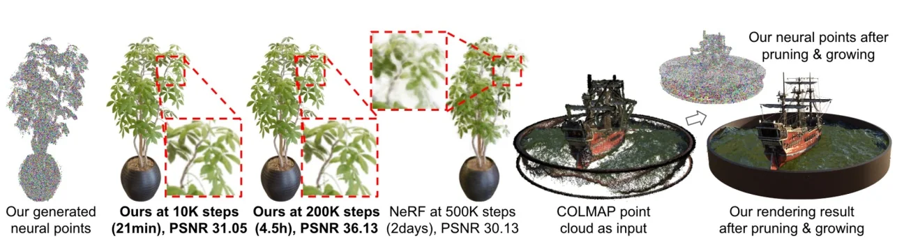
Method
Overview Point-NeRF reconstructs a continuous radiance field by augmenting an explicit 3D point set with neural attributes and rendering it with a lightweight, local MLP. Crucially, the 3D points and their initial attributes are obtained by scene-independent, feed-forward networks that operate directly on posed images—so a new scene can be initialized relatively fast without re-training these networks.
Inputs. We are given a calibrated image set \[ \mathcal {I}_Q=\{(I_q,\Phi _q)\}_{q=1}^{Q},\quad \Phi _q=(K_q,R_q,t_q), \] i.e., \(Q\) RGB images with known intrinsics/extrinsics.
Scene-independent initialization (learned across many scenes). Point-NeRF trains two modules across scenes so they generalize to new inputs and provide a fast, scene-agnostic initialization:
-
Geometry/Confidence module \(G_{p,\gamma }\) (MVSNet-style 3D CNN). For a reference view \(q\) with a small set of neighboring source views \(\mathcal {N}(q)\) (typically \(|\mathcal {N}(q)|{=}2\)), \(G_{p,\gamma }\) proceeds as follows:
- 1.
- Plane-swept cost volume. Build a 3D tensor over \((u,v,d)\) by differentiably warping source-view feature maps onto fronto-parallel planes placed at discrete depths \(d\!\in \!\mathcal {D}\) in the reference frustum (plane-induced homographies). At each pixel \((u,v)\) and plane \(d\), we compute a cost (e.g., channel-wise variance across the warped sources) that measures multi-view agreement. Intuition: if the hypothesized plane passes through the true surface seen at \((u,v)\), the warped source features align well and the cost is low; otherwise they disagree and the cost is high.
- 2.
- Regularization and probabilities. A compact 3D CNN regularizes the noisy cost volume and outputs depth logits \(L_q(u,v,d)\); applying a softmax along \(d\) gives the depth probability volume \[ P_q(u,v,d)=\frac {\exp L_q(u,v,d)}{\sum _{d'\in \mathcal {D}}\exp L_q(u,v,d')}\in [0,1],\quad \sum _{d\in \mathcal {D}} P_q(u,v,d)=1. \] Intuition: the logits are unnormalized scores; after softmax, \(P_q(u,v,\cdot )\) becomes a distribution along the reference ray stating how likely each depth hypothesis explains pixel \((u,v)\) given all views.
- 3.
- Depth regression (soft-argmin). Regress a single expected depth per pixel by the probability-weighted average \[ D_q(u,v)=\sum _{d\in \mathcal {D}} d\,P_q(u,v,d). \] Intuition: \(D_q(u,v)\) is the (differentiable) expectation of the per-ray depth distribution. If \(P_q(u,v,\cdot )\) is sharply peaked at some \(d^\star \), then \(D_q(u,v)\!\approx \!d^\star \) (like an argmax); if it is spread over nearby planes, \(D_q\) interpolates them, yielding sub-plane precision.
- 4.
- Unprojection to 3D points. Using the reference camera parameters \(\Phi _q=(K_q,R_q,t_q)\), back-project each pixel \((u,v)\) with depth \(d=D_q(u,v)\) into 3D: \[ x_{\mathrm {cam}}=d\,K_q^{-1}[u,v,1]^\top ,\qquad p=R_q^{\!\top }(x_{\mathrm {cam}}-t_q)\in \mathbb {R}^3, \] producing a per-view point set \(\{p_i^{(q)}\}_{i=1}^{N_q}\). Intuition: this lifts the 2D depth map \(D_q\) into a cloud of 3D anchors that sit on the most plausible surface along each reference ray.
- 5.
- Confidence from \(P_q\). Assign each 3D point a confidence by sampling the depth probability at its inferred depth: \[ \gamma _i^{(q)}\approx P_q\!\big (u_i,\,v_i,\,D_q(u_i,v_i)\big )\in [0,1], \] using tri-linear interpolation in \((u,v,d)\) to handle non-integer coordinates. Intuition: tri-linear sampling blends the eight neighboring grid values to evaluate \(P_q\) at the continuous location \((u_i,v_i,d_i)\). If \(P_q(u_i,v_i,\cdot )\) is peaked near \(d_i\), the pixel’s multi-view evidence strongly agrees there, so \(\gamma _i^{(q)}\) is large; if it is flat or multi-modal, the depth is uncertain and \(\gamma _i^{(q)}\) is small.
Generalization. Trained once across diverse scenes, \(G_{p,\gamma }\) produces dense geometry and uncertainty-aware confidences for a new scene with a single forward pass (no per-scene retraining), yielding a fast and reliable geometric scaffold for Point-NeRF.
- Feature module \(G_f\) (2D CNN). Independently, \(G_f\) extracts multi-scale feature maps from each \(I_q\) (shared weights across views). For every 3D point \(p_i^{(q)}\), we project it into visible training views and sample the corresponding feature maps; the sampled descriptors are fused (e.g., concatenation/averaging or a small fusion MLP) to obtain a per-point appearance vector \(f_i^{(q)}\). \(G_f\) is also trained across scenes and reused as-is at inference.
Running \(G_{p,\gamma }\) and \(G_f\) for several references yields per-view sets \(\{(p_i^{(q)},f_i^{(q)},\gamma _i^{(q)})\}\). These are combined (union with light filtering/deduplication) into a single, scene-level neural point cloud \[ P=\{(p_i,f_i,\gamma _i)\mid i=1,\dots ,N\}, \] which then drives fast, surface-aware rendering and the subsequent per-scene refinement (with pruning and growing).
Per-scene refinement (\(\approx \) tens of minutes). Given the unified neural point cloud \(P=\{(p_i,f_i,\gamma _i)\}_{i=1}^N\) (points \(p_i\!\in \!\mathbb {R}^3\) with per-point features \(f_i\) from \(G_f\) and confidences \(\gamma _i\)), Point-NeRF renders a novel view by differentiable ray marching restricted to space near the point cloud. This restriction avoids wasting samples in empty regions and is implemented by querying, at each shading location, only the \(K\) nearest neural points within a radius \(R\). All radiance and density predictions at shading locations are regressed from these local neighbors rather than a global MLP.
Ray setup and sampling (as in NeRF) For a target camera with intrinsics \(K\) and extrinsics \((R,t)\) (world\(\to \)camera), a pixel \((u,v)\) defines a camera ray with origin at the camera center \(o=-R^{\!\top }t\) and direction \[ d \;=\; \frac {R^{\!\top }K^{-1}[u,\,v,\,1]^\top }{\big \|R^{\!\top }K^{-1}[u,\,v,\,1]^\top \big \|}. \] We sample depths \(\{t_j\}_{j=1}^{M}\) along this ray (near\(\to \)far) and form shading locations \(x_j=o+t_j d\) with spacings \(\Delta _j=t_{j+1}-t_j\). The pixel color is accumulated via the standard volume-rendering rule \[ c \;=\; \sum _{j=1}^{M}\tau _j\!\left (1-e^{-\sigma _j\Delta _j}\right )\, r_j, \qquad \tau _j \;=\; \exp \!\Big (-\sum _{t=1}^{j-1}\sigma _t\Delta _t\Big ). \] Intuition. At each sample \(x_j\) the density \(\sigma _j\) induces an opacity \(\alpha _j=1-e^{-\sigma _j\Delta _j}\) (how much the sample contributes) and a transmittance \(\tau _j\) (how much light survives from the ray origin up to \(x_j\)). The emitted/view-dependent color \(r_j\) is then weighted by the chance that the ray reaches \(x_j\) (\(\tau _j\)) and “stops” there (\(\alpha _j\)). High \(\sigma _j\) increases \(\alpha _j\) (more contribution, more occlusion downstream); low \(\sigma _j\) passes energy forward.
Local neighbor query (surface-aware shading) At each ray sample \(x_j\) we gather only the \(K\) nearest anchors within a radius \(R\): \[ \mathcal {N}(x_j)\;=\;\Big \{(p_i,f_i,\gamma _i)\ \Big |\ \|p_i-x_j\|\le R,\ \mbox{$K$ nearest}\Big \}. \] Restricting computation to nearby anchors focuses shading near likely surfaces and avoids wasting samples in empty space. In practice, a uniform voxel grid or hash grid over \(\{p_i\}\) accelerates neighbor lookup so that only cells intersected by the ray are visited.
Local feature regression (Eq. 3) Each neighbor \((p_i,f_i,\gamma _i)\in \mathcal {N}(x_j)\) is turned into a location-specific descriptor by a small MLP \(F\): \[ f_{i,x_j}\;=\;F\!\big (f_i,\;x_j-p_i\big ). \] Conditioning on the relative offset \(x_j-p_i\) (with positional encoding in practice) grants translation invariance and lets each neural point act as a local 3D chart around itself.
Radiance aggregation (Eqs. 4–5) Location-specific features are blended with inverse-distance weights and confidence modulation: \[ f_{x_j}\;=\;\frac {\sum _{i}\gamma _i\,w_i\,f_{i,x_j}}{\sum _i w_i}, \qquad w_i=\frac {1}{\|x_j-p_i\|}, \qquad r_j\;=\;R\!\big (f_{x_j},\,d\big ), \] where \(R\) is a light MLP that also takes the viewing direction \(d\) (directional positional encoding). Intuition: nearby, high-confidence anchors dominate \(r_j\), while distant or dubious anchors are downweighted.
Density aggregation (Eqs. 6–7) Densities are produced in two stages: \[ \sigma _i \;=\; T\!\big (f_{i,x_j}\big ),\qquad \sigma _j\;=\;\frac {\sum _i \sigma _i\,\gamma _i\,w_i}{\sum _i w_i}, \quad w_i=\frac {1}{\|x_j-p_i\|}. \] Why both \(w_i\) and \(\gamma _i\)? \(w_i\) encodes geometric proximity (even a reliable point should not dominate far away), while \(\gamma _i\) encodes reliability (even a nearby point should contribute little if its confidence is low). Together they yield robust, surface-aware \(\sigma _j\).
Putting the pieces together For each pixel ray: (i) sample \(\{x_j\}\), (ii) query \(\mathcal {N}(x_j)\), (iii) compute \(\{f_{i,x_j}\}\) via \(F\), (iv) aggregate to \(r_j\) and \(\sigma _j\) via \(R\) and \(T\), and (v) composite with \[ c \;=\; \sum _{j=1}^{M}\tau _j\!\left (1-e^{-\sigma _j\Delta _j}\right )\, r_j, \qquad \tau _j \;=\; \exp \!\Big (-\sum _{t=1}^{j-1}\sigma _t\Delta _t\Big ). \]
End-to-end optimization objective Rendered colors are supervised by an \(\ell _2\) photometric loss \(L_{\mbox{render}}\) (optionally plus perceptual terms). During per-scene refinement, gradients do flow into the neural point cloud attributes and the local shading MLPs, while the scene-agnostic generators \(G_{p,\gamma }\) and \(G_f\) remain frozen (they were pretrained across scenes to provide fast initialization). Concretely, we update:
- Per-point attributes \((f_i,\gamma _i)\): \(f_i\) specializes to the scene’s appearance; \(\gamma _i\) sharpens so anchors truly on-surface receive high confidence while outliers are suppressed.
- Local MLPs \(F,R,T\): adapt the mapping from neighbor-conditioned features to \((r,\sigma )\) for this scene.
- Topology (discrete edits): instead of moving \(p_i\) continuously (unstable and unable to close large holes), we use pruning and growing.
The total loss is \[ L_{\mbox{total}} \;=\; L_{\mbox{render}} \;+\; \lambda _{\mbox{sparse}}\,L_{\mbox{sparse}}, \qquad L_{\mbox{sparse}} ~=~ \frac {1}{|\gamma |}\sum _i\!\big [\log (\gamma _i)+\log (1-\gamma _i)\big ], \] which (per paper Eq. (10)) polarizes confidences toward \(\{0,1\}\) and makes pruning decisions unambiguous.
Topology edits during refinement (per paper) Pruning. Points with persistently low confidence are removed; specifically, every \(10\mathrm {K}\) iterations, points with \(\gamma _i<0.1\) are pruned (as in the paper), eliminating outliers and reducing neighborhood clutter.
Growing. To add anchors where geometry is missing, use the current field to propose new points along training rays. For a sample at \(x_j\) with density \(\sigma _j\) and step \(\Delta _j\), define the instantaneous opacity \[ \alpha _j \;=\; 1 - \exp (-\sigma _j \Delta _j). \] Let \(j_g=\arg \max _j \alpha _j\) be the most opaque sample on the ray (paper Eq. (11)). If (i) \(\alpha _{j_g}\) exceeds an opacity threshold \(T_{\mbox{opacity}}\) (likely surface) and (ii) the distance from \(x_{j_g}\) to the nearest existing anchor exceeds \(T_{\mbox{dist}}\) (under-anchored region), insert a new point at \(p_{\mbox{new}}=x_{j_g}\). Initialize its attributes as in the paper’s pipeline: features \(f_{\mbox{new}}\) from \(G_f\) by projecting \(p_{\mbox{new}}\) into visible views and fusing sampled descriptors; confidence \(\gamma _{\mbox{new}}\) with a moderate prior (e.g., \(0.3\)) that will be driven by \(L_{\mbox{render}}{+}L_{\mbox{sparse}}\). Merging near-duplicates and updating the neighbor index keeps queries efficient.
Outcome. Because geometry and initial descriptors come from the pretrained, scene-independent generators (\(G_{p,\gamma }\) and \(G_f\)), per-scene training converges in tens of minutes yet achieves quality competitive with or better than NeRF trained for hours. The confidence- and distance-weighted aggregation stabilizes learning, while pruning/growing self-organize the anchor set to close holes and remove outliers, preparing us for the next section on Architecture & Implementation Details.
Architecture and Implementation Details
- Point Generation: Depth maps predicted via a cost-volume 3D CNN \(G_{p,\gamma }\), unprojected into 3D points with confidence \(\gamma _i\).
- Feature Extraction: 2D CNN \(G_f\) (VGG-style) produces multi-scale features aligned with points.
- Radiance/Density MLPs: Small per-point MLPs regress local features, radiance, and density.
- Positional Encoding: Applied to relative positions and view directions.
- Optimization: Loss combines rendering error and sparsity penalty: \[ L_{\mbox{opt}} = L_{\mbox{render}} + \alpha L_{\mbox{sparse}}, \] with pruning/growing every 10k iterations.
Experiments and Ablations
Point-NeRF is evaluated on DTU [273], NeRF-Synthetic [442], Tanks&Temples [311], and ScanNet [115]. This section reproduces the paper’s reported numbers and highlights the main observations.
No Per-scene Optimization | Per-scene Optimization |
||||||||
|---|---|---|---|---|---|---|---|---|---|
| PixelNeRF [762] | MVSNeRF [79] | IBRNet [677] | Point-NeRF | Point-NeRF\(_{\!1\mathrm {K}}\) | Point-NeRF\(_{\!10\mathrm {K}}\) | MVSNeRF\(_{\!10\mathrm {K}}\) | IBRNet\(_{\!10\mathrm {K}}\) | NeRF\(_{\!200\mathrm {K}}\) [442] | |
| PSNR \(\uparrow \) | 19.31 | 26.63 | 26.04 | 23.89 | 28.43 | 30.12 | 28.50 | 31.35 | 27.01 |
| SSIM \(\uparrow \) | 0.789 | 0.931 | 0.917 | 0.874 | 0.929 | 0.957 | 0.933 | 0.956 | 0.902 |
| LPIPS\(_{\mathrm {VGG}}\) \(\downarrow \) | 0.382 | 0.168 | 0.190 | 0.203 | 0.183 | 0.117 | 0.179 | 0.131 | 0.263 |
| Time \(\downarrow \) | – | – | – | – | 2min | 20min | 24min | 1h | 10h |
DTU With \(1\mbox{K}\) iterations (\(\approx 2\) minutes), Point-NeRF already exceeds a NeRF baseline at \(200\mbox{K}\) iterations (\(\approx 10\) hours) on PSNR/SSIM/LPIPS; at \(10\mbox{K}\) iterations it attains the best SSIM and LPIPS among the listed methods (Table 1).
| NPBG [8] | NeRF [442] | IBRNet [677] | NSVF [379] | Point-NeRF\(^{\mathrm {col}}_{\!200\mathrm {K}}\) | |
| Point-NeRF\(_{\!20\mathrm {K}}\) Point-NeRF\(_{\!200\mathrm {K}}\) | |||||
| PSNR \(\uparrow \) | 24.56 | 31.01 | 28.14 | 31.75 | 31.77 30.71 33.31 |
| SSIM \(\uparrow \) | 0.923 | 0.947 | 0.942 | 0.964 | 0.973 0.967 0.978 |
| LPIPS\(_{\mathrm {VGG}}\) \(\downarrow \) | 0.109 | 0.081 | 0.072 | – | 0.062 0.081 0.049 |
| LPIPS\(_{\mathrm {Alex}}\) \(\downarrow \) | 0.095 | – | – | 0.047 | 0.040 0.050 0.027 |
NeRF-Synthetic At \(20\mbox{K}\) iterations (\(\approx 40\) minutes), Point-NeRF reaches NeRF-level quality; at \(200\mbox{K}\) it surpasses NeRF on PSNR/SSIM/LPIPS (Table 2), with qualitative advantages on thin structures.
Tanks&Temples and ScanNet On the Tanks&Temples subset of [311] (five scenes: Ignatius, Truck, Barn, Caterpillar, Family), Point-NeRF reports a mean \(29.61\) / \(0.954\) / \(0.080\) (PSNR / SSIM / LPIPS\(_\mbox{Alex}\)), which improves over NSVF’s \(28.40\) / \(0.900\) / \(0.153\) by \(+1.21\) dB PSNR, \(+0.054\) SSIM, and \(-0.073\) LPIPS (lower is better), indicating higher fidelity and better perceptual quality under larger, real scenes.
For ScanNet [115] (two scenes used by [379]), Point-NeRF achieves \(30.32\) / \(0.909\) / \(0.220\) versus NSVF’s \(25.48\) / \(0.688\) / \(0.301\), i.e., \(+4.84\) dB PSNR, \(+0.221\) SSIM, and \(-0.081\) LPIPS\(_\mbox{Alex}\). These results follow the evaluation protocol of [379] (depth-image–initialized scenes) and show a consistent advantage in both accuracy and perceptual metrics on indoor scans.
Initialization from external COLMAP clouds When starting from COLMAP points [571], pruning and growing (Sec. 23.10.8.0) substantially improve geometry and rendering. The following figure shows qualitative effects; The following table (paper’s numbers) reports gains on Ship and Hotdog.
| Method | Ship (PSNR / SSIM / LPIPS\(_{\mbox{VGG}}\)) | Hotdog (PSNR / SSIM / LPIPS\(_{\mbox{VGG}}\)) |
|---|---|---|
| Point-NeRF (No P&G) | 25.50 / 0.878 / 0.182 | 34.91 / 0.983 / 0.067 |
| Point-NeRF (With P&G) | 30.97 / 0.942 / 0.124 | 37.30 / 0.991 / 0.037 |
| COLMAP init (No P&G) | 19.35 / 0.905 / 0.167 | 29.91 / 0.978 / 0.061 |
| COLMAP init (With P&G) | 30.18 / 0.941 / 0.134 | 35.49 / 0.986 / 0.061 |
Feature-initialization ablation (paper’s Table 5) Initializing point features with extracted multi-view image features accelerates convergence and improves final metrics versus random initialization: 20K iters PSNR/SSIM \(30.09/0.963\) (extracted) vs. \(25.44/0.932\) (random); 200K iters \(33.00/0.978\) (extracted) vs. \(32.01/0.972\) (random).
Limitations
- Dependence on seed quality. The feed-forward initializer greatly accelerates setup, but extremely sparse or noisy initial geometry can still cap fidelity. Pruning/growing helps, yet very large holes or heavy outliers remain challenging to repair quickly.
- Memory and neighborhood queries. High point densities increase memory footprint and the cost of building/querying spatial indices. At render time, each shaded sample performs a local \(K\)NN aggregation, so throughput is ultimately limited by ray marching and repeated neighbor lookups.
- Mesh extraction. Even though the representation is anchored by explicit points, producing watertight, topologically consistent meshes from the learned radiance field is non-trivial, as in many radiance-field methods.
Outlook toward 3D Gaussian Splatting. These bottlenecks motivate alternative explicit radiance parameterizations that trade local \(K\)NN aggregation and per-sample MLP evaluations for analytic rasterization of continuous primitives. A prominent next step is 3D Gaussian Splatting [299], which represents the scene with anisotropic Gaussians carrying color (e.g., spherical-harmonics coefficients), opacity, and covariance. Rendering then becomes screen-space splatting with differentiable visibility, enabling much higher frame rates. In the following section, a comparison is drawn between Point-NeRF’s point-anchored, ray-marched formulation and Gaussian-based splatting, clarifying how the latter alleviates neighbor-query overhead and amortizes rendering—while introducing its own visibility and ordering considerations.
Enrichment 23.10.9: 3D Gaussian Splatting: RT Radiance Field Rendering
Motivation and big picture
Context and objective Radiance fields deliver high-fidelity novel views, but classic NeRF pipelines are costly at train and render time due to dense ray marching and repeated MLP evaluation. Fast explicit variants (Plenoxels, DVGO, Instant-NGP, TensoRF, etc.) accelerate this by replacing networks with explicit features or compact encodings, while Point-NeRF adopts point primitives with differentiable rasterization. 3D Gaussian Splatting (3DGS) [299] represents the scene with anisotropic 3D Gaussians and renders them using a visibility-aware, differentiable, tile-based software rasterizer. Each 3D ellipsoid projects to a 2D ellipse whose Gaussian footprint is blended front-to-back, preserving the volumetric accumulation behavior while enabling real-time rendering once optimized.
Key idea 3D Gaussian Splatting (3DGS) renders scenes by forward rasterization instead of backward ray marching [299]. The scene is a collection of learnable anisotropic 3D Gaussians. Each Gaussian is projected to a soft 2D ellipse and blended in front-to-back depth order using \(\alpha \)-compositing; this reproduces volumetric visibility while remaining GPU-friendly.
Core terms A 3D Gaussian is defined by a center \(\mu \in \mathbb {R}^3\) and covariance \(\Sigma \in \mathbb {R}^{3\times 3}\) with (unnormalized) density \[ G(x)\;\propto \;\exp \!\Big (-\tfrac {1}{2}(x-\mu )^{\top }\Sigma ^{-1}(x-\mu )\Big ). \] If \(\Sigma =\sigma ^2 I\) the spread is the same in all directions (isotropic); otherwise it is direction-dependent and the shape is an oriented ellipsoid (anisotropic). 3DGS parameterizes the covariance in a sophisticated manner allowing simple optimization with minimal constraints.
How 3DGS uses Gaussians Each Gaussian stores:
- geometry and opacity: \((\mu ,\,R,\,S,\,a)\).
- appearance: a set of learned spherical harmonics (SH) coefficients for view-dependent color.
All parameters are optimized from posed images via backpropagation (details later).
From 3D to 2D footprints We use the standard pinhole camera to map a 3D point to pixel coordinates. Let a world point be \(x\in \mathbb {R}^3\). First apply the extrinsics \(W=[R_c\,|\,t_c]\) (world\(\to \)camera): \[ X \;=\; W\,\tilde {x} \;=\; \begin {bmatrix} X_c \\ Y_c \\ Z_c \end {bmatrix}, \qquad \tilde {x}=\begin {bmatrix}x\\1\end {bmatrix}, \] so \((X_c,Y_c,Z_c)\) are the point’s coordinates in the camera frame and \(Z_c{>}0\) is its depth along the optical axis. Then apply the intrinsics \[ K \;=\; \begin {bmatrix} f_x & 0 & c_x\\[2pt] 0 & f_y & c_y\\[2pt] 0 & 0 & 1 \end {bmatrix}, \] where \(f_x,f_y\) are focal lengths measured in pixels (scaling image-space units along \(u\) and \(v\)), and \((c_x,c_y)\) is the principal point (optical center in pixels). The pinhole projection \(\pi :\mathbb {R}^3\to \mathbb {R}^2\) is \[ (u,v) \;=\; \pi (X) \;=\; \Bigl (f_x\,\tfrac {X_c}{Z_c} + c_x,\;\; f_y\,\tfrac {Y_c}{Z_c} + c_y\Bigr ), \] i.e., we form normalized image coordinates \((X_c/Z_c,\,Y_c/Z_c)\) and then scale/shift by \((f_x,f_y)\) and \((c_x,c_y)\).
Local linearization and the projection Jacobian To obtain a simple, differentiable footprint for each Gaussian, we linearize the pixel coordinates near its center \(\mu \). Let \(X_0=W\,\mu =(X_0,Y_0,Z_0)^{\top }\) be the center in camera space. The projection Jacobian \(J\in \mathbb {R}^{2\times 3}\) is the derivative of pixel coordinates with respect to camera coordinates at \(X_0\): \[ J \;=\; \left .\frac {\partial (u,v)}{\partial (X_c,Y_c,Z_c)}\right |_{X_0} \;=\; \begin {bmatrix} \dfrac {f_x}{Z_0} & 0 & -\,\dfrac {f_x X_0}{Z_0^2}\\[10pt] 0 & \dfrac {f_y}{Z_0} & -\,\dfrac {f_y Y_0}{Z_0^2} \end {bmatrix}. \] Thus a small 3D motion \(\delta X\) near \(X_0\) produces a pixel shift \(\delta p\approx J\,\delta X\): lateral moves \((X_c,Y_c)\) shift pixels by roughly \(f_{x,y}/Z_0\) (more at small depth, less when far), while motion along \(Z_c\) changes scale, pushing pixels outward as the point approaches the camera.
Induced 2D covariance Gaussian covariances transform under a linear map \(A\) as \(A\,\Sigma \,A^{\top }\). Since a small world-space displacement \(\delta x\) maps to pixels by \(\delta p\approx (J\,W)\,\delta x\), the screen-space covariance is \[ \Sigma ' \;=\; J\,W\,\Sigma \,W^{\top }J^{\top }. \] Geometrically, the 3D ellipsoid becomes a 2D ellipse whose orientation and size encode local perspective (rotation, foreshortening, scale). This \(\Sigma '\) defines a soft, rapidly decaying footprint over nearby pixels; farther from the ellipse center, the contribution to the pixel is smaller.
View-dependent color with spherical harmonics For a fixed view, each projected ellipse contributes one RGB color; only its per-pixel weight \(\alpha _i(x)\) varies across the footprint. That color is a function on directions \(\hat {\mathbf {v}}_i=(o-\mu _i)/\|o-\mu _i\|\in \mathbb {S}^2\) and is expanded in real spherical harmonics (an orthonormal basis on the unit sphere, analogous to a Fourier/Taylor basis but for directions): \[ c_i(\hat {\mathbf {v}}_i)=\sum _{l=0}^{L}\sum _{m=-l}^{l}\mathbf {c}_{i,lm}\,Y_{lm}(\hat {\mathbf {v}}_i), \] where \(Y_{lm}\) are basis functions on \(\mathbb {S}^2\) and \(\mathbf {c}_{i,lm}\!\in \!\mathbb {R}^3\) are learned per-Gaussian coefficients. Low degrees \(L\) capture smooth, low-frequency view dependence; higher \(L\) add directional detail. Training starts at \(L{=}0\) (constant color) to stabilize geometry and opacity, then ramps \(L\) up (e.g., to a small order) to introduce view dependence without a large decoder [299].
Rasterize and composite For each view, 3DGS projects all Gaussians, sorts overlapping footprints front-to-back within image tiles, and blends them using \(\alpha \)-compositing. If \(\alpha _k(x)\) is the per-pixel opacity of the \(k\)-th (depth-sorted) Gaussian at pixel \(x\), and \(c_k\) is its view-dependent color, the accumulated color uses the transmittance \(T_{k-1}(x)\) (remaining visibility before \(k\)): \[ C(x)\;=\;\sum _k T_{k-1}(x)\,\alpha _k(x)\,c_k,\qquad T_k(x)\;=\;T_{k-1}(x)\,\bigl (1-\alpha _k(x)\bigr ),\quad T_0(x)=1. \] This reproduces the effect of volumetric rendering but operates on 2D ellipses (no per-ray samples).
- Quality with compactness Anisotropic Gaussians align to edges and thin structures, achieving sharp detail with fewer primitives (vs. isotropic point splats or uniformly sampled ray accumulations).
- Surface alignment and subpixel fidelity Oriented ellipses capture anisotropic image gradients (edges, ridges), reducing holes and flicker compared with Point-NeRF and classic NeRF.
- Explicit visibility with dense gradients Front-to-back \(\alpha \)-compositing gives crisp occlusion ordering, and the differentiable rasterizer sends gradients to many overlapping splats per pixel, avoiding k-nearest sparsity and per-ray sample sparsity.
- Efficient view dependence Per-Gaussian spherical harmonics (SH) produce smooth directional color without a large MLP; degree ramping stabilizes early training. [299].
- Capacity steering in 3D The clone/split/prune schedule adapts both the number and the shape/orientation of primitives, concentrating dof where reprojection errors are high.
- Real-time rendering 2D rasterization on projected ellipses replaces expensive ray marching.
- Tile-wise global ordering A single radix sort by depth and tile enables coherent front-to-back blending with early termination once transmittance saturates.
- Stable, fast optimization The covariance parameterization and closed-form projection to \(\Sigma '\) yield well-behaved gradients; analytic derivatives for the parameters avoid fragile PSD constraints and heavy autodiff through eigendecompositions.
In what follows we derive 3DGS step by step, and then then turn to experiments and ablations, and conclude with limitations and follow-up work.
3D Gaussian Splatting stages
Before we dive into the details, we give a high-level walkthrough of the 3DGS pipeline, linking the core idea—forward rasterization of anisotropic 3D Gaussians—to the concrete steps used for projection, image formation, optimization, and real-time rendering.
- 1.
- Initialization From calibrated multi-view images, run SfM to recover camera poses and a sparse point cloud. Seed one Gaussian per SfM point with center \(\mu \), rotation \(R\) (via a unit quaternion), diagonal scale \(S=\mathrm {diag}(s_x,s_y,s_z)\), opacity \(a\), and a small set of real spherical-harmonics (SH) coefficients for view-dependent color. For stability, begin with degree \(L{=}0\) (constant color) and ramp \(L\) upward as geometry and opacity settle.
- 2.
- Projection Around each center \(\mu \), locally linearize the pinhole camera. With world\(\to \)camera transform \(W\) and the \(2{\times }3\) projection Jacobian \(J\) at \(W\mu \), the 3D covariance \(\Sigma =(RS)(RS)^{\top }\) becomes the screen-space covariance \[ \Sigma ' \;=\; J\,W\,\Sigma \,W^{\top }J^{\top }. \] Thus a 3D ellipsoid projects to a soft 2D ellipse (splat) with image mean \(u=\pi (W\mu )\). The camera-space depth \(Z_c\) of \(\mu \) will define visibility order.
- 3.
- Image formation For pixel \(x\), each overlapping splat contributes a weight (opacity) that decays with its elliptical distance: \[ \alpha _i(x)\;\propto \; a_i\,\exp \!\Big (-\tfrac {1}{2}(x-u_i)^{\top }{\Sigma _i'}^{-1}(x-u_i)\Big ). \] The splat’s color is evaluated once per view from its SH expansion at the unit view direction \(\hat {\mathbf {v}}_i=(o-\mu _i)/\|o-\mu _i\|\): \[ c_i(\hat {\mathbf {v}}_i)\;=\;\sum _{l=0}^{L}\sum _{m=-l}^{l}\mathbf {c}_{i,lm}\,Y_{lm}(\hat {\mathbf {v}}_i). \] Splat colors are then accumulated using front-to-back \(\alpha \)-compositing: \[ C(x)\;=\;\sum _{k} T_{k-1}(x)\,\alpha _k(x)\,c_k,\qquad T_k(x)\;=\;T_{k-1}(x)\bigl (1-\alpha _k(x)\bigr ),\quad T_0(x)=1. \] Why front-to-back Gaussians are processed from nearest to farthest (increasing \(Z_c\)). This respects occlusions (near splats naturally hide far ones) and enables early termination: once \(T_{k-1}(x)\) becomes very small (pixel nearly opaque), remaining far splats can be skipped, saving work without changing the result.
- 4.
- Optimization and adaptive densification Optimize all parameters \((\mu ,R,S,a,\) SH\()\) end-to-end with Adam under a photometric loss (typically L1 + SSIM). Every few iterations, apply density control to match detail to error signals: clone small Gaussians in high-gradient regions (under-reconstruction), split over-large splats into two smaller ones when gradients suggest unresolved structure, and prune nearly transparent or excessively large Gaussians. The SH degree \(L\) is increased during training so view dependence is learned after geometry stabilizes.
- 5.
- Real-time rendering A GPU tile-based differentiable rasterizer frustum-culls Gaussians, bins them into fixed-size tiles (e.g., \(16{\times }16\)), globally sorts by (tile, depth), and blends per-pixel in front-to-back order. The visibility-aware order gives correct occlusion and allows early-out when transmittance saturates; a compact backward pass records only touched splats for gradients. Together these yield real-time novel-view synthesis once trained.
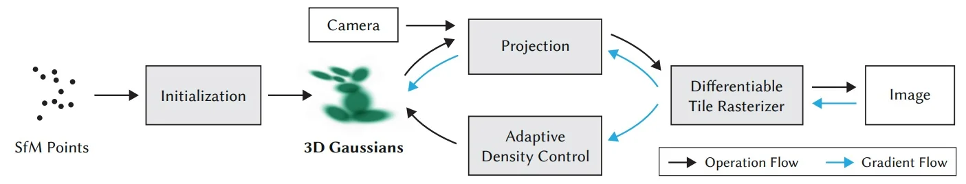
Representation and parameterization
From mean–covariance to a renderable primitive A 3D Gaussian is specified by a mean \(\mu \in \mathbb {R}^3\) and a covariance \(\Sigma \in \mathbb {R}^{3\times 3}\), with (unnormalized) density \[ G(x)\;\propto \;\exp \!\Big (-\tfrac 12(x-\mu )^\top \Sigma ^{-1}(x-\mu )\Big ). \] The quadratic form \((x-\mu )^\top \Sigma ^{-1}(x-\mu )\) acts like a squared distance (the Mahalanobis distance). Let \(\Sigma =Q\Lambda Q^\top \) be the eigendecomposition, where \(Q=[e_1\ e_2\ e_3]\) has unit, mutually orthogonal columns (the principal directions) and \(\Lambda =\mathrm {diag}(\lambda _1,\lambda _2,\lambda _3)\) with \(\lambda _i\ge 0\) (the principal variances). Then:
- Principal directions \(e_i\) are unit vectors in \(\mathbb {R}^3\) that define the ellipsoid’s axes. They coincide with the canonical \(x/y/z\) axes only if \(\Sigma \) is already diagonal in that basis. In general, \(e_i\) are rotated versions of \(x/y/z\).
- Level sets are the sets of points where the density has the same value, equivalently where the Mahalanobis distance is constant: \[ \{\,x\in \mathbb {R}^3 : (x-\mu )^\top \Sigma ^{-1}(x-\mu )=k\,\}\quad (k>0). \] In 3D these level sets are ellipsoids centered at \(\mu \) with semi–axis lengths \(\sqrt {k\,\lambda _i}\) along directions \(e_i\). The constant \(k\) simply picks “how far out” the surface is (larger \(k\) \(\Rightarrow \) a larger, similar ellipsoid). Intuitively, you can think of \(k\) as selecting a “constant–standard–deviation” contour, generalized to 3D.
- Isotropy vs. anisotropy If \(\Sigma =\sigma ^2 I\), then \(e_i\) align with \(x/y/z\) and all \(\lambda _i=\sigma ^2\), producing a sphere (isotropic spread). If the \(\lambda _i\) differ and/or \(Q\neq I\), the ellipsoid is stretched and rotated (anisotropic spread).
In practical terms, increasing a variance (some \(\lambda _i\)) makes the ellipsoid longer along the corresponding principal direction \(e_i\); introducing covariance (nonzero off–diagonals in \(\Sigma \)) rotates the principal directions away from \(x/y/z\). After local projection to the image, these adjustments control the width and orientation of the resulting 2D ellipse (the screen–space footprint).
Initialization and the need for valid, optimizable covariances 3DGS initializes one Gaussian per SfM point to cover the coarse geometry, then continuously optimizes the set while adding, cloning, splitting, and pruning primitives (densification) as required by the data [299]. During training, every covariance must remain a valid covariance (symmetric and positive semidefinite): \[ \Sigma =\Sigma ^\top ,\qquad x^\top \Sigma \,x\ge 0\ \ \forall x. \] Naively updating the free entries of \(\Sigma \) can violate these constraints (e.g., negative eigenvalues), destabilizing learning and yielding non-physical shapes. A parameterization that preserves validity by construction is therefore essential.
Choosing a geometry parameterization for valid optimization As directly updating the parameters of the covariance matrix \(\Sigma \) can violate symmetry or positive semidefiniteness (PSD), which destabilizes learning. 3DGS instead optimizes a decoupled set of variables and reconstructs \(\Sigma \) from them: \[ (\mu ,\,R,\,S)\quad \mbox{with}\quad \Sigma \;=\; R\,S\,S^\top R^\top , \] where
- \(\mu \in \mathbb {R}^3\) is the 3D center (learned by gradient descent).
- \(R\in \mathbb {R}^{3\times 3}\) is a rotation matrix (\(R^\top R=I,\ \det (R)=1\)) obtained from a unit quaternion that is re-normalized after each update.
- \(S=\mathrm {diag}(s_x,s_y,s_z)\) holds positive axis scales (enforced via a positivity reparameterization, e.g., \(\exp \) or sigmoid activation).
Because \(S S^\top \) is PSD and \(R\) is orthonormal, \(R S S^\top R^\top \) is always symmetric PSD, so validity is guaranteed throughout training—no eigen-clamping or PSD projection is needed. Equally important, this form decouples orientation (\(R\)) from axis lengths (\(S\)), yielding interpretable, well-conditioned updates; in contrast, editing \(\Sigma \) directly entangles rotation and scale (off-diagonals simultaneously tilt and shear), making gradients harder to interpret and constrain. The paper also provides closed-form derivatives w.r.t. the scale and quaternion parameters, avoiding fragile eigendecompositions.
Intuition and practical knobs for \(R\) and \(S\) Think of \(S\) as the axis lengths and \(R\) as the steering wheel that orients those axes in space:
- Vary \(s_x\) or \(s_y\) (with \(R\) fixed) stretches or shrinks the ellipsoid along the corresponding rotated axes in world space. After projection the screen-space ellipse widens mainly along the matching image directions, helping one primitive cover elongated features (e.g., edges) with fewer neighbors.
- Vary \(s_z\) (depth thickness) increases extent roughly along the view-normal direction, adding controllable thickness. This improves coverage of slanted, foreshortened surfaces across nearby views and reduces holes.
- Rotate \(R\) (with \(S\) fixed) re-orients the ellipsoid without changing its radii. The projected ellipse rotates accordingly, letting a single primitive align with wires, leaf stems, fence slats, or oblique edges—capturing anisotropic detail compactly and reducing flicker.
These independent knobs let 3DGS tilt, stretch, and thicken coverage to match local geometry in 3D while keeping every covariance valid during optimization.
Opacity as a direct parameter 3DGS replaces NeRF’s ray–integrated density with a per–Gaussian opacity that directly gates the screen–space footprint. For Gaussian \(i\) we keep an unconstrained logit \(\tilde a_i\in \mathbb {R}\) and map it to a bounded opacity \[ a_i \;=\; \sigma (\tilde a_i) \;=\; \frac {1}{1+e^{-\tilde a_i}} \in (0,1), \] optionally clamped to \(a_i\in [\varepsilon ,\,1-\varepsilon ]\) (e.g., \(\varepsilon =10^{-3}\)) for numerical stability.
After projection, the ellipse has center \(u_i\) and screen–space covariance \(\Sigma _i'\). Its per–pixel alpha (used in compositing) is the unnormalized Gaussian falloff scaled by \(a_i\): \[ \alpha _i(x)\;=\;a_i\;\exp \!\Bigl (-\tfrac {1}{2}\,(x-u_i)^\top {\Sigma _i'}^{-1}(x-u_i)\Bigr ). \] Thus \(\alpha _i(u_i)=a_i\) and \(\alpha _i(x)\le a_i<1\) elsewhere. Colors are then blended in front–to–back order using the transmittance recursion, which both respects occlusion and enables early termination once the remaining visibility is negligible [299].
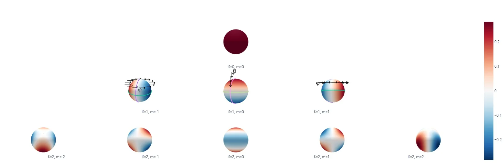
How to read Fig. 23.72 and why SH suit 3DGS. Directions live on the unit sphere \(\mathbb {S}^2\), and \(\{Y_{\ell m}\}\) form an orthonormal basis, much like Fourier modes on a circle.
- Degree \(\ell \): sets angular resolution. Larger \(\ell \) means more bands in \(\theta \) (north–south).
- Order \(m\): sets azimuthal detail. \(|m|\) counts nodal meridians in \(\phi \) (east–west), while \(\ell -|m|\) counts nodal circles in \(\theta \).
Examples in Fig. 23.72:
-
\(\ell =0\) (monopole):
- \(m=0\): constant everywhere, no variation.
-
\(\ell =1\) (dipoles):
- \(m=-1\): varies left–right with \(\phi \), one vertical nodal plane; vanishes at poles.
- \(m=0\): varies up–down with \(\theta \), node at the equator (north pole red, south pole blue).
- \(m=1\): same as \(m=-1\) but rotated \(90^\circ \) around \(z\).
-
\(\ell =2\) (quadrupoles):
- \(m=-2\): four lobes around the equator, separated by two vertical nodal planes (\(90^\circ \) apart); zeros at poles.
- \(m=-1\): four lobes alternating across equator and meridian; one vertical plane and one horizontal circle as nodes.
- \(m=0\): two polar caps of one sign and an equatorial belt of the opposite sign; nodal circles at \(\cos ^2\theta =\tfrac {1}{3}\).
- \(m=1\): same as \(m=-1\) but rotated \(90^\circ \) in \(\phi \).
- \(m=2\): same as \(m=-2\) but rotated \(90^\circ \) in \(\phi \).
This basis is ideal for 3D Gaussian Splatting: the view direction \(\hat {\mathbf v}\) lies on \(\mathbb {S}^2\), and a low-order SH expansion provides a compact, smooth, differentiable way to represent each Gaussian’s view-dependent color.
Appearance as a directional color field For a fixed camera, each projected ellipse contributes one RGB that depends on the unit view direction \(\hat {\mathbf v}=(o-\mu )/\|o-\mu \|\in \mathbb {S}^2\). 3DGS models this per channel with a real spherical–harmonics (SH) expansion \[ \begin {aligned} c^{(r)}(\hat {\mathbf v})&=\sum _{l=0}^{L}\sum _{m=-l}^{l} c^{(r)}_{lm}\,Y_{lm}(\hat {\mathbf v}),\qquad c^{(g)}(\hat {\mathbf v})=\sum _{l=0}^{L}\sum _{m=-l}^{l} c^{(g)}_{lm}\,Y_{lm}(\hat {\mathbf v}),\\ c^{(b)}(\hat {\mathbf v})&=\sum _{l=0}^{L}\sum _{m=-l}^{l} c^{(b)}_{lm}\,Y_{lm}(\hat {\mathbf v}), \end {aligned} \] so there are \((L{+}1)^2\) coefficients per channel (e.g., \(L{=}2\) uses \(9\) per channel, \(27\) total). Real SH form an orthonormal basis on directions.
Practical intuition.
- \(L{=}0\) (only \(Y_{00}\)): view–independent “clay ball” color; good for diffuse walls or matte plastic.
- \(L{\approx }1\mbox{–}2\): broad, smooth directional changes (fabric sheen, brushed metal, soft grazing–angle brightening).
- \(L{\approx }2\mbox{–}3\): sharper lobes suitable for glossy paint/ceramic and weak specular highlights.
Very mirror–like effects would require still higher \(L\), but 3DGS typically keeps \(L\) small for compactness and stability.
Coarse–to–fine SH ramping for stable training. Rather than enable full view dependence from the start, 3DGS trains with a curriculum [299]:
- 1.
- Begin with \(L{=}0\) (diffuse). Color is direction–independent, so the optimizer must first fit images via geometry \((\mu ,R,S)\) and opacity \(a\)—reducing “cheating” with spurious view effects and limiting floaters.
- 2.
- Unlock higher \(L\) in stages. After geometry/opacity stabilize, enable \(L{=}1,2,\ldots \) to add higher angular frequencies (specular–like lobes, Fresnel–like changes) without destabilizing the coarse structure. This mirrors frequency annealing used in other neural rendering systems and yields robust geometry first, then progressively richer view dependence with only a handful of extra coefficients.
Image formation and compositing
What each splat provides For a pixel \(x\) and for every Gaussian \(i\) whose footprint reaches it, we already have:
- Its screen–space mean \(u_i\) and covariance \(\Sigma '_i\) (the ellipse).
- Its per–pixel alpha \(\alpha _i(x)\) (peak opacity \(a_i\) modulated by the elliptical falloff; Sec. 23.10.9.0).
- Its view–dependent RGB \(c_i\) evaluated once for the current camera using SH.
Depth ordering for visibility Occlusion is handled by sorting contributors at \(x\) from nearest to farthest using their camera–space depths \(Z_{c,i}\) at the Gaussian centers \(\mu _i\). This establishes a visibility–aware sequence \(k=1,2,\dots \).
Front–to–back transmittance (premultiplied form) Let \(T_{k-1}(x)\) be the remaining visibility before blending the \(k\)-th (already depth–sorted) splat. Using premultiplied colors, \[ C(x)\;=\;\sum _{k} T_{k-1}(x)\,\alpha _k(x)\,c_k,\qquad T_k(x)\;=\;T_{k-1}(x)\bigl (1-\alpha _k(x)\bigr ),\quad T_0(x)=1. \]
- Near splats contribute first; farther ones are attenuated by \(T_{k-1}(x)\).
- This mirrors volumetric rendering, but on projected 2D ellipses rather than per–ray samples (NeRF: \(T=\exp (-\!\int \sigma \,ds)\); here \(\alpha \) acts as discrete absorption).
Why front–to–back matters now The transmittance recursion is causal: \(T_k\) depends only on earlier alphas. Consequently, \[ \mbox{if}\;\;T_{k-1}(x)\le \varepsilon _T \;\Rightarrow \; \sum _{j\ge k} T_{j-1}(x)\,\alpha _j(x)\,\|c_j\| \;\le \; \varepsilon _T, \] since \(\alpha _j\in [0,1]\) and \(\|c_j\|\le 1\) (normalized colors). Two immediate consequences:
- Occlusion is respected by construction: Near content attenuates or completely hides far content as \(T\) decreases.
- The remaining sum is bounded once \(T\) is small: A pixel “pre–finishes”, so later terms are negligible. We will exploit this property when describing early termination in the rasterizer.
Practical footprint (compact support) Although a Gaussian has infinite support, its tail is negligible beyond a few standard deviations. Define the elliptical distance \[ d_i^2(x)\;=\;(x-u_i)^\top {\Sigma '_i}^{-1}(x-u_i), \] and restrict evaluation to \(x\) inside a level set \(\{\,d_i^2(x)\le \tau \,\}\) (e.g., \(\tau \in [3,5]\)). This:
- Focuses computation where the splat meaningfully contributes.
- Avoids numerical noise from summing vanishingly small tails.
Where we are headed. The equations above define the image formation the renderer must realize. We next complete the method—adaptive densification and optimization (losses, gradients)—then return to the tile–based rasterizer, which enforces depth order and leverages the transmittance pre–finish for efficiency.
Adaptive densification
Goal and signal Starting from one Gaussian per SfM point, we adaptively allocate capacity so primitives concentrate where reprojection error persists. Every \(K\) iterations (e.g., a few hundred), we consult view-space positional gradients \(\nabla _{\mu }\mathcal {L}\) and simple shape statistics to decide whether to clone, split, or prune. This keeps the model compact while resolving missing detail [299].
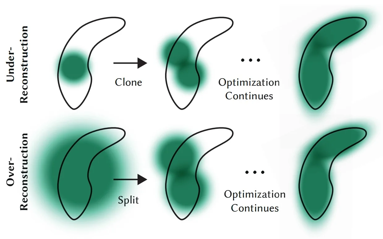
Clone (add coverage) If a small splat (e.g., bounded principal axes in \(S\) and screen footprint in \(\Sigma '\)) exhibits a large view-space positional gradient \(\|\nabla _{\mu }\mathcal {L}\|\) over recent iterations, we clone it:
- 1.
- Create a copy with the same \((R,S,a,\mbox{SH})\).
- 2.
- Displace the clone’s center by a small step along the aggregated gradient direction (optionally normalized and scaled).
- 3.
- Optionally damp the parent/clone opacities slightly to avoid transient over-coverage.
Cloning increases local sample density where the renderer still fails to match image evidence (thin structures, high-curvature silhouettes).
Split (resolve detail) If a splat remains large (e.g., one axis of \(S\) above a threshold) while residuals stay high, we split:
- 1.
- Replace the parent by two children whose scales are reduced by a factor \(\phi \) (empirically \(\phi {\approx }1.6\)) along all axes.
- 2.
- Sample child centers from the parent’s 3D Gaussian (or place them symmetrically along the principal axis with largest spread).
- 3.
- Inherit \((R,a,\mbox{SH})\), optionally perturb \(R\) or \(S\) minutely to break symmetry.
Splitting preserves coverage but increases spatial frequency capacity, allowing edges and textures to be represented with multiple smaller footprints.
Prune (stay compact) We prune primitives that contribute negligibly or become degenerate:
- Nearly transparent (\(a\) below a threshold over a window of iterations).
- Unreasonably large in world space or screen space (guard against splats that try to “cover everything”).
- Persistently off-frustum or behind the near plane.
Pruning reduces memory and compute and prevents artifacts such as low-contrast haze.
When and how often Densification runs periodically and touches only a fraction of splats per pass. Thresholds for gradient magnitude, size (via \(S\) or \(\Sigma '\) eigenvalues), and opacity are set conservatively; exact values can be tuned per dataset, but the logic—clone if small & underfit, split if large & underfit, prune if unused or degenerate—follows [299]. Because gradients propagate through the differentiable rasterizer to all overlapping splats, these decisions are well informed by multi-view evidence.
Effect on optimization Interleaving gradient steps with densification yields a coarse-to-fine growth of representation: the model first captures broad layout, then allocates more, smaller, and better-oriented Gaussians only where error persists. This shares the spirit of multiresolution strategies in explicit grids, but preserves the flexibility of an unstructured point-based representation.
Training objective and schedules
Photometric objective We fit rendered images to ground truth using a convex combination of per-pixel \(\ell _1\) and a differentiable SSIM-based term: \[ \mathcal {L}(C,\,C^\star )\;=\;(1-\lambda )\,\|C-C^\star \|_1\;+\;\lambda \,\mathrm {D\mbox{-}SSIM}(C,\,C^\star ), \qquad \lambda \in [0,1], \] where \(C\) is the rendered image and \(C^\star \) the target. The SSIM component measures luminance, contrast, and structure agreement in local windows, providing a perceptual anchor that complements the edge-preserving \(\ell _1\) term.
SSIM, D-SSIM, and the notion of “structure” For two local patches \(x,y\) (e.g., Gaussian-weighted \(11{\times }11\) windows), SSIM is \[ \mathrm {SSIM}(x,y) =\frac {(2\mu _x\mu _y + C_1)(2\sigma _{xy}+C_2)} {(\mu _x^2+\mu _y^2 + C_1)(\sigma _x^2+\sigma _y^2 + C_2)}, \] where:
- Luminance match \((2\mu _x\mu _y + C_1)/(\mu _x^2+\mu _y^2 + C_1)\) compares local means (exposure/brightness).
- Contrast match \((2\sigma _x\sigma _y + C_2)/(\sigma _x^2+\sigma _y^2 + C_2)\) compares local standard deviations (contrast).
- Structure match is essentially the normalized correlation \(\sigma _{xy}/(\sigma _x\sigma _y)\); it rewards the same pattern of variation even when absolute intensity shifts slightly.
We turn similarity into a loss via \(\mathrm {D\mbox{-}SSIM}(x,y)=(1-\mathrm {SSIM}(x,y))/2\in [0,1]\), averaged over windows and channels. In practice, SSIM’s structure term encourages the correct spatial relationships of pixels (textures, edges, fine detail), while the luminance/contrast terms keep exposure and local energy consistent. See [467, 25] for practical guidance.
Why not pure MSE/PSNR Mean squared error (MSE) underlies PSNR (\(\mathrm {PSNR}=-10\log _{10}\mathrm {MSE}\)) but correlates poorly with human visual perception: it penalizes small spatial shifts of high-frequency content excessively and often prefers blurry predictions over slightly misaligned sharp ones. In 3DGS, many overlapping splats jointly explain high-frequency detail; a pure MSE/PSNR objective tends to over-smooth such detail. The \(\ell _1{+}\)D-SSIM blend better matches HVS (Human Vision System) sensitivity: \(\ell _1\) preserves edges, while SSIM emphasizes local structural fidelity (textures, contrasts) and tolerates mild brightness drifts.
LPIPS vs. SSIM in training LPIPS [800] compares images in a deep feature space (e.g., VGG/AlexNet), and is strong as an evaluation metric for perceptual quality. We do not use LPIPS in the 3DGS training loss for several reasons:
- Photometric faithfulness matters. Supervision comes from posed photos; exact colors and fine correspondences are crucial for stable geometry/opacity learning. LPIPS has feature invariances that can tolerate color/brightness shifts, sometimes encouraging “perceptually OK” but photometrically biased reconstructions.
- Efficiency and memory. LPIPS requires a forward/backward pass through a deep CNN per image (or patch), adding nontrivial compute and VRAM on top of the differentiable rasterizer. SSIM is lightweight and fully local.
- Gradient locality and stability. SSIM provides short-range, structure-aligned gradients that integrate well with splat-based compositing; LPIPS offers non-local gradients that can destabilize early optimization (especially before geometry has converged).
Empirically, \(\ell _1{+}\)D-SSIM (with a small \(\lambda \), e.g., \(0.2\) as in [299]) yields sharp, photometrically faithful results while keeping training fast and stable. LPIPS remains valuable for reporting perceptual quality at test time.
Update schedule and stability We optimize all parameters \((\mu ,R,S,a,\mbox{SH})\) with Adam over mini-batches of posed images.
- Learning rates. Slightly larger for \((\mu ,S)\) early to quickly settle geometry; smaller for rotation (quaternion) and SH to avoid oscillations.
- SH degree ramping. Keep \(L{=}0\) (view-independent color) until geometry/opacity stabilize, then unlock \(L{=}1,2,\ldots \) in stages. This coarse-to-fine curriculum first fixes layout and coverage, then adds higher angular frequencies (specular-like lobes, Fresnel-like variation) without destabilizing structure [299].
- Opacity hygiene. Clamp \(a\in [\varepsilon ,1-\varepsilon ]\) and optionally apply periodic small resets near the cameras to discourage persistent semi-transparent “floaters” before pruning.
Differentiable tile–based rasterizer
Goal and inputs The rasterizer must realize the image–formation equations from Sec. 23.10.9.0 efficiently on GPU, while preserving differentiability. For the current view we assume, per Gaussian \(i\), the following are already available:
- Screen–space mean \(u_i\) and covariance \(\Sigma '_i\).
- Peak opacity \(a_i\) and per–pixel alpha definition \(\alpha _i(x)\).
- View–dependent color \(c_i\) evaluated once from SH for this camera.
- Camera–space depth \(Z_{c,i}\) at the center \(\mu _i\) (for visibility ordering).
- Frustum–cull Gaussians whose ellipses lie fully outside the image (use a conservative \(d_i^2(x)\le \tau \) mask).
- For each remaining Gaussian, compute the tight axis–aligned bounding box of its ellipse level set \(\{x:\,d_i^2(x)\le \tau \}\) and clip it to the screen.
Stage B: tile binning Partition the screen into fixed–size tiles (e.g., \(16{\times }16\)). For each Gaussian \(i\):
- Determine the set of tiles overlapped by its clipped ellipse box.
- Emit a record for each overlapped tile \(t\): a pair \((i,t)\) plus the quantities needed downstream (e.g., \(u_i\), \({\Sigma '_i}^{-1}\), \(a_i\), \(c_i\), \(Z_{c,i}\)).
Stage C: global sort by (tile, depth) Construct a 64–bit key per record \((i,t)\) that packs
- The tile id in the most significant bits (groups records by tile).
- A monotone depth key derived from \(Z_{c,i}\) in the least significant bits (orders front–to–back).
Globally radix–sort all records by this key; the result is a single array where each tile occupies a contiguous segment with its Gaussians in front–to–back order.
Stage D: per–tile blending (forward) Launch one CUDA block per tile; within a block, assign one thread per pixel. For the tile’s ordered list \((i_1,\dots ,i_M)\):
- Initialize \(C(x){:=}\mathbf {0}\) and \(T(x){:=}1\) for every pixel \(x\) in the tile.
-
For \(m=1\ldots M\):
- Compute the elliptical distance \(d_{i_m}^2(x)\) and skip if \(d_{i_m}^2(x)>\tau \) (compact support).
- Evaluate \(\alpha _{i_m}(x)=a_{i_m}\exp (-\tfrac 12 d_{i_m}^2(x))\).
- Accumulate \(C(x)\mathrel {+}= T(x)\,\alpha _{i_m}(x)\,c_{i_m}\).
- Update \(T(x)\mathrel {*}=(1-\alpha _{i_m}(x))\).
- Optionally stop if \(T(x)\le \varepsilon _T\) (front–to–back “pre–finish”).
Minimal bookkeeping for backprop. While iterating, each pixel thread appends a compact record for every touched splat \(i_m\): store its index, \(T_{m-1}(x)\) (the prefix transmittance just before blending), and \(\alpha _{i_m}(x)\). This per–pixel visitation list is short due to compact support and pre–finish, and suffices for an efficient backward pass.
Stage E: per–tile gradients (backward) Given pixel–wise loss gradients \(\frac {\partial \mathcal {L}}{\partial C(x)}\in \mathbb {R}^3\), traverse each pixel’s visitation list in reverse order to accumulate parameter derivatives. Let the \(k\)–th visited (depth–sorted) splat at \(x\) have \((i_k,\,T_{k-1}(x),\,\alpha _{i_k}(x),\,c_{i_k})\), and define the suffix “background color” seen behind \(k\) (normalized) by the recurrence \[ \bar C_{\mbox{behind}}^{(K+1)}(x)=\mathbf {0},\qquad \bar C_{\mbox{behind}}^{(k)}(x)=\alpha _{i_k}(x)\,c_{i_k}\;+\;\bigl (1-\alpha _{i_k}(x)\bigr )\,\bar C_{\mbox{behind}}^{(k+1)}(x). \] Then for each \(k\) (from back to front):
- Color coefficients (SH) receive \[ \frac {\partial \mathcal {L}}{\partial c_{i_k}} \mathrel {+}= T_{k-1}(x)\,\alpha _{i_k}(x)\;\frac {\partial \mathcal {L}}{\partial C(x)}. \]
- Opacity (per–pixel) receives \[ \frac {\partial \mathcal {L}}{\partial \alpha _{i_k}(x)} \mathrel {+}= T_{k-1}(x)\;\Bigl (\,c_{i_k}\;-\;\bar C_{\mbox{behind}}^{(k+1)}(x)\Bigr )\,\cdot \,\frac {\partial \mathcal {L}}{\partial C(x)}. \]
- Chain to geometric parameters via \(\alpha _{i_k}(x)=a_{i_k}\exp (-\tfrac 12 d_{i_k}^2(x))\): \[ \frac {\partial \mathcal {L}}{\partial a_{i_k}} \mathrel {+}= \exp \!\bigl (-\tfrac 12 d_{i_k}^2(x)\bigr )\;\frac {\partial \mathcal {L}}{\partial \alpha _{i_k}(x)},\qquad \frac {\partial \mathcal {L}}{\partial d_{i_k}^2(x)} \mathrel {+}= -\tfrac 12\,\alpha _{i_k}(x)\;\frac {\partial \mathcal {L}}{\partial \alpha _{i_k}(x)}. \]
- Propagate \(\frac {\partial \mathcal {L}}{\partial d^2}\) to \(u_{i_k}\) and \(\Sigma '_{i_k}\) using \[ d_{i_k}^2(x)=(x-u_{i_k})^\top {\Sigma '_{i_k}}^{-1}(x-u_{i_k}), \] and then further to world–space \((\mu ,R,S)\) through the Jacobian chain \(\Sigma ' = J W \Sigma W^\top J^\top \).
Because only touched pairs \((x,i)\) are revisited, the backward pass scales with the effective overlap, not the total number of Gaussians.
Numerical and implementation notes
- Tile size. \(16{\times }16\) balances occupancy and shared–memory usage; other sizes are possible.
- Stable alphas. Keep \(a_i\in [\varepsilon ,1-\varepsilon ]\) and use \(\tau \in [3,5]\) for compact support (Sec. 23.10.9.0).
- Recompute vs. store. To minimize memory, store \(T_{k-1}\) and \(\alpha _{i_k}(x)\); re–evaluate \(c_{i_k}\) from SH on the fly if needed (one evaluation per splat–pixel).
- Sparse work. Frustum culling, compact support, and pre–finish together bound both forward work and the size of visitation lists, enabling real–time rendering once trained.
Summary. The rasterizer maps the analytic 2D ellipse footprints to tiles, establishes a per–tile, front–to–back order with a single global sort, and evaluates the premultiplied \(\alpha \)–compositing recurrence using only local (tile) data. A compact per–pixel record of touched splats permits an equally local backward pass, with gradients chained to opacity, color (SH), and geometry through closed–form derivatives. This completes the forward/backward machinery of 3DGS.
Experiments and ablations
Datasets and evaluation protocol Evaluation is conducted on widely used real and synthetic benchmarks:
- Mip-NeRF360 [28]: real, unbounded 360\(^\circ \) captures with large baselines and substantial depth variation (e.g., Bicycle, Garden, Stump, Counter, Room). The official train/test splits are used.
- Tanks&Temples [311]: real outdoor/vehicle scenes with challenging occlusions and scale changes (commonly Truck, Train) and accurate ground-truth poses.
- Deep Blending [222]: real indoor environments (Playroom, DrJohnson) exhibiting complex view-dependent effects and clutter, with calibrated multi-view imagery.
- Synthetic NeRF (Blender) [442]: rendered objects with clean geometry and known ground truth (Chair, Drums, Ficus, Hotdog, Lego, Materials, Mic, Ship) for controlled comparisons.
Unless otherwise noted, images are rendered at each dataset’s standard resolution. Reported metrics are PSNR (dB; higher is better), SSIM (\(\uparrow \)), and LPIPS (\(\downarrow \)). Optimization wall-clock time and novel-view FPS are reported on a single high-end GPU, following the protocol of [299].
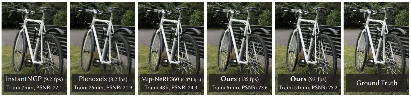
Quantitative comparison (held-out views) We summarize cross-dataset results (reformatted into per-dataset tables for readability).
| Method | SSIM \(\uparrow \) | PSNR \(\uparrow \) | LPIPS \(\downarrow \) | Train | FPS | Mem |
| Plenoxels | 0.626 | 23.08 | 0.463 | 25m49s | 6.79 | 2.1GB |
| INGP-Base | 0.671 | 25.30 | 0.371 | 5m37s | 11.7 | 13MB |
| INGP-Big | 0.699 | 25.59 | 0.331 | 7m30s | 9.43 | 48MB |
| Mip-NeRF360 | 0.792\(^\dagger \) | 27.69\(^\dagger \) | 0.237\(^\dagger \) | 48h | 0.06 | 8.6MB |
| 3DGS-7K | 0.770 | 25.60 | 0.279 | 6m25s | 160 | 523MB |
| 3DGS-30K | 0.815 | 27.21 | 0.214 | 41m33s | 134 | 734MB |
| Method | SSIM \(\uparrow \) | PSNR \(\uparrow \) | LPIPS \(\downarrow \) | Train | FPS | Mem |
| Plenoxels | 0.719 | 21.08 | 0.379 | 25m05s | 13.0 | 2.3GB |
| INGP-Base | 0.723 | 21.72 | 0.330 | 5m26s | 17.1 | 13MB |
| INGP-Big | 0.745 | 21.92 | 0.305 | 6m59s | 14.4 | 48MB |
| Mip-NeRF360 | 0.759 | 22.22 | 0.257 | 48h | 0.14 | 8.6MB |
| 3DGS-7K | 0.767 | 21.20 | 0.280 | 6m55s | 197 | 270MB |
| 3DGS-30K | 0.841 | 23.14 | 0.183 | 26m54s | 154 | 411MB |
| Method | SSIM \(\uparrow \) | PSNR \(\uparrow \) | LPIPS \(\downarrow \) | Train | FPS | Mem |
| Plenoxels | 0.795 | 23.06 | 0.510 | 27m49s | 11.2 | 2.7GB |
| INGP-Base | 0.797 | 23.62 | 0.423 | 6m31s | 3.26 | 13MB |
| INGP-Big | 0.817 | 24.96 | 0.390 | 8m00s | 2.79 | 48MB |
| Mip-NeRF360 | 0.901 | 29.40 | 0.245 | 48h | 0.09 | 8.6MB |
| 3DGS-7K | 0.875 | 27.78 | 0.317 | 4m35s | 172 | 386MB |
| 3DGS-30K | 0.903 | 29.41 | 0.243 | 36m02s | 137 | 676MB |
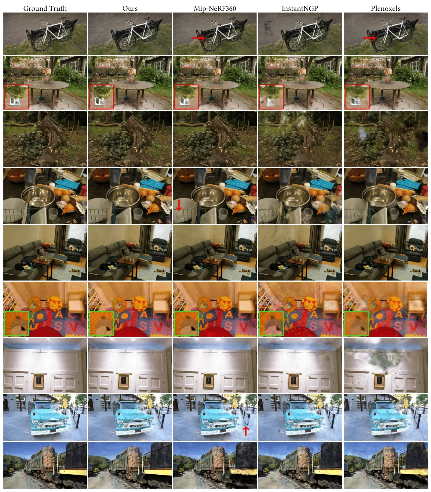
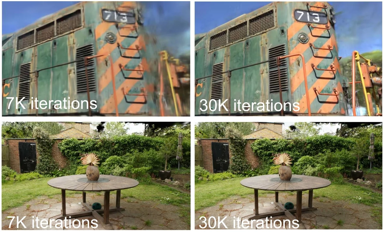
| Method | Mic | Chair | Ship | Materials | Lego | Drums | Ficus | Hotdog | Avg. |
| Plenoxels | 33.26 | 33.98 | 29.62 | 29.14 | 34.10 | 25.35 | 31.83 | 36.81 | 31.76 |
| INGP-Base | 36.22 | 35.00 | 31.10 | 29.78 | 36.39 | 26.02 | 33.51 | 37.40 | 33.18 |
| Mip-NeRF | 36.51 | 35.14 | 30.41 | 30.71 | 35.70 | 25.48 | 33.29 | 37.48 | 33.09 |
| Point-NeRF | 35.95 | 35.40 | 30.97 | 29.61 | 35.04 | 26.06 | 36.13 | 37.30 | 33.30 |
| 3DGS-30K | 35.36 | 35.83 | 30.80 | 30.00 | 35.78 | 26.15 | 34.87 | 37.72 | 33.32 |
Ablations We study design choices via controlled ablations (numbers reproduced from [299]).
| Setting | Truck-5K | Garden-5K | Bicycle-5K | Truck-30K | Garden-30K | Bicycle-30K | Avg-5K | Avg-30K |
| Limited-BW | 14.66 | 22.07 | 20.77 | 13.84 | 22.88 | 20.87 | 19.16 | 19.19 |
| Random Init | 16.75 | 20.90 | 19.86 | 18.02 | 22.19 | 21.05 | 19.17 | 20.42 |
| No-Split | 18.31 | 23.98 | 22.21 | 20.59 | 26.11 | 25.02 | 21.50 | 23.90 |
| No-SH | 22.36 | 25.22 | 22.88 | 24.39 | 26.59 | 25.08 | 23.48 | 25.35 |
| No-Clone | 22.29 | 25.61 | 22.15 | 24.82 | 27.47 | 25.46 | 23.35 | 25.91 |
| Isotropic | 22.40 | 25.49 | 22.81 | 23.89 | 27.00 | 24.81 | 23.56 | 25.23 |
| Full | 22.71 | 25.82 | 23.18 | 24.81 | 27.70 | 25.65 | 23.90 | 26.05 |
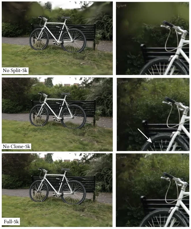
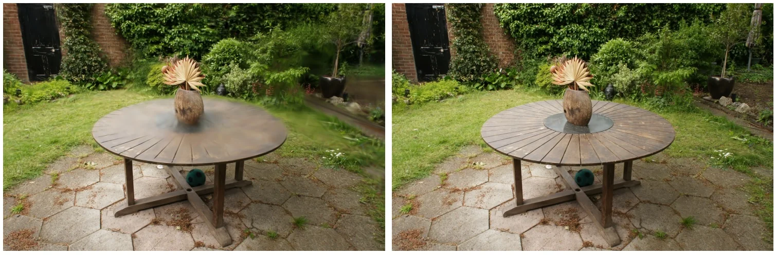
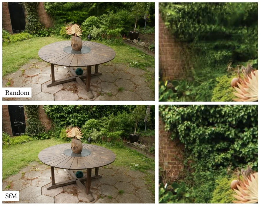
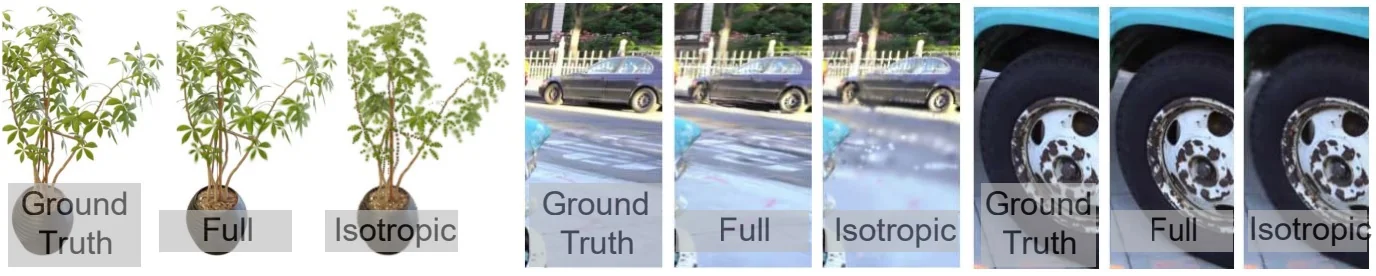
- Quality vs. speed: With tens of minutes of training, 3DGS approaches or surpasses Mip-NeRF360 quality while enabling real-time novel-view rendering (\(\ge \!100\) FPS) on standard GPUs.
- Representation matters: Anisotropy, view-dependent SH, and densification (clone/split) each contribute significantly; removing any one harms PSNR/visual fidelity (Table 23.19).
- Initialization helps: SfM seeding outperforms random starts, reducing artifacts and time to quality (Fig. 23.79).
Limitations and future work
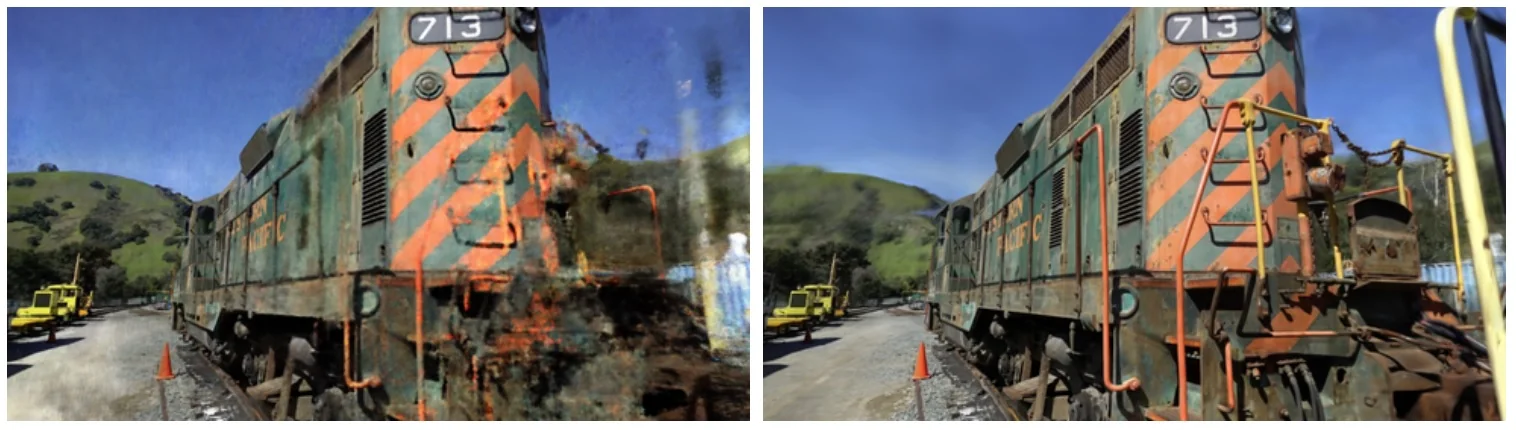
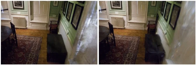
Typical limitations include:
- Sparse coverage or weak overlap. With limited multi-view support, Gaussians may overgrow (coarse blobs) or under-cover (holes), especially at long range [299, 28].
- Extreme view dependence. Very sharp, mirror-like effects exceed low-degree SH; capturing such specularities robustly requires richer reflectance models [299].
- Memory scaling. Quality grows with the number of Gaussians; very large scenes can stress memory bandwidth and capacity without compression or streaming [299].
- Static-scene assumption. The base formulation targets rigid, static scenes; handling motion or changing illumination requires extensions beyond the original 3DGS pipeline [299].
Future work Recent, highly cited follow-ups suggest concrete avenues beyond the original formulation:
- Dynamics and tracking. Extending splats to time (4D) enables real-time dynamic rendering [725], while dense SLAM systems fuse mapping and tracking directly with Gaussians for online reconstruction [551].
- Richer appearance / inverse rendering. Jointly estimating reflectance and lighting with Gaussian splats (inverse rendering) improves specularities and relighting fidelity [702]; surfel-style anisotropic primitives further tighten shading–geometry coupling [298].
- Initialization and scalability. Removing reliance on external SfM (e.g., COLMAP-free pipelines) widens applicability and can reduce failure cases tied to sparse/biased points [164]; generative priors with Gaussians help regularize learning and scale content creation [627].
- Surfaces and hybrids. Surface-aligned or surface-extractable Gaussian formulations bridge to mesh-like structure for editing and compression [200], complementing the original unstructured point representation.
Enrichment 23.11: NeRF: Real-World Robustness & Sparse Supervision
NeRFs trained “in the wild” must tolerate sparse viewpoints, photometric variation, and even unknown poses. These works inject priors or jointly estimate calibration to make NeRFs usable under realistic capture.
- BARF [360]: Jointly optimizes camera poses and NeRF via coarse-to-fine (frequency) scheduling, reducing local minima in self-calibration.
- NeRF-W [431]: Handles unconstrained photo collections by separating “transient” appearance (lighting, people) from static scene content.
- IBRNet [677]: A generalizable IBR prior that conditions on a few source views to synthesize novel views without per-scene MLP overfitting.
- PixelNeRF [762]: Predicts scene radiance directly from one/few images using a CNN encoder, enabling few-shot generalization.
Further influential works (not expanded): RegNeRF [466] (regularization for sparse inputs), Mega-NeRF [426] (distributed training at landscape scale).
Enrichment 23.11.1: BARF: Bundle-Adjusting Neural Radiance Fields
Motivation and problem setting
Why this problem matters Neural Radiance Fields (NeRF) achieve high-fidelity novel-view synthesis only if all training images come with accurate camera extrinsics. In real captures, however, poses from SfM/SLAM can be noisy, incomplete, or entirely unavailable (e.g., monocular videos, sparse photo collections). This dependency limits NeRF in exactly the regimes we care about for robust, real-world deployment: casual capture, small baselines, texture-poor scenes, or motion that confounds SfM. Removing the reliance on precomputed poses would unlock NeRF for far broader use.
What makes joint optimization hard If poses are inaccurate or unknown, training becomes a coupled problem over the scene and the cameras. Naïvely unfreezing poses in a standard NeRF objective turns the problem highly nonconvex and initialization-sensitive: the network can explain photometric errors either by moving the cameras or by hallucinating geometry/appearance. In practice this often yields misregistered trajectories, distorted geometry, and rendering artifacts instead of self-correction [360]. The core need is to shape the optimization so that early gradients provide coherent, consistent directions for camera updates.
A lesson from classical image alignment In classical registration, direct photometric methods optimize geometric parameters and routinely employ multiscale image pyramids to enlarge the basin of convergence. The strategy is to first align low-frequency (blurred or downsampled) images to obtain a robust global displacement, and only then reintroduce higher-frequency detail for refinement. Low-pass residuals yield smoother objectives and coherent gradients; exposing high frequencies too early makes the landscape rugged and per-pixel Jacobians oscillatory, impeding convergence. BARF transfers this multiscale idea from images to neural fields by low-passing the inputs—via a schedule that gates NeRF’s positional-encoding bands during training—so early pose updates are governed by smooth structure and fine detail is deferred until registration stabilizes.
The paper’s idea and contribution BARF reframes NeRF with unknown poses as dense photometric bundle adjustment and makes it tractable by controlling frequency content. Concretely, it:
- Jointly optimizes camera poses and the radiance field under the standard rendering loss.
- Applying a smooth coarse-to-fine window over positional-encoding bands that enlarges the basin for pose recovery and only later restores full representational bandwidth. This simple mechanism reliably realigns cameras from noisy or identity initializations and preserves NeRF-level fidelity once all bands are active.
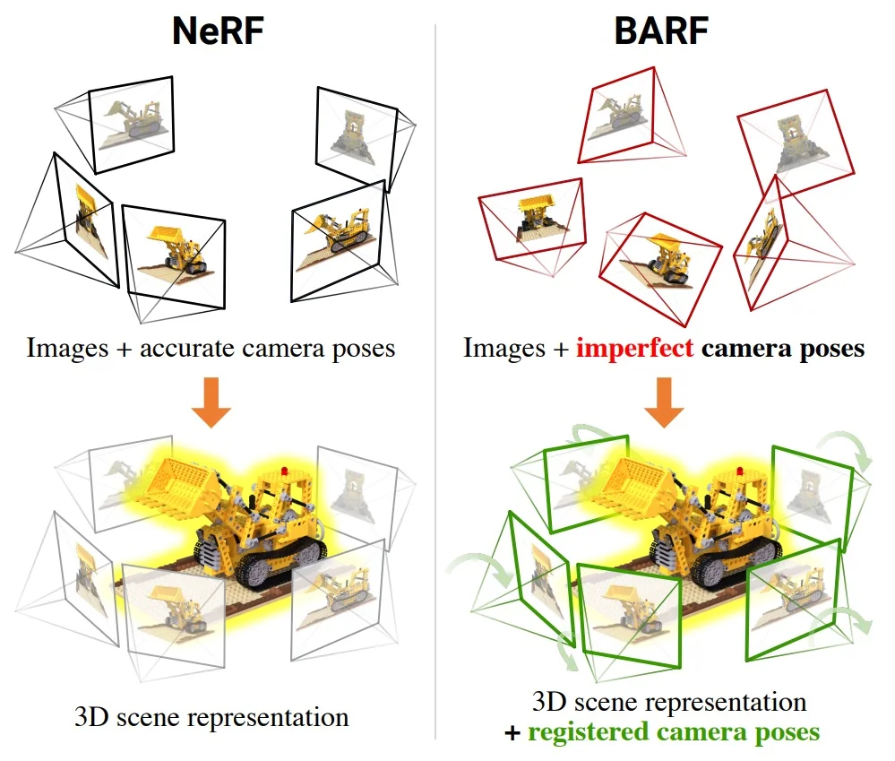
What we aim to solve and why:
- Goal — Learn a high-fidelity neural scene and accurate camera poses directly from images, without relying on external SfM/SLAM.
- Challenge — Naïve joint optimization is ill-conditioned: high-frequency encodings inject rugged gradients that drive poses to poor local minima.
- Approach — Window the frequency bands of positional encoding in a coarse-to-fine schedule so early pose gradients are stable and globally coherent.
- Impact — Makes NeRF usable with imperfect/unknown poses, recovering trajectories from scratch and achieving view synthesis competitive with pose-supervised NeRFs [360].
High level overview of BARF
Joint objective Given images \(\{I_i\}_{i=1}^M\) and a radiance field \(f_\theta \) mapping a 3D location and a view direction to density and color, \[ f_\theta :\;(\mathbf {x},\mathbf {d}) \;\mapsto \; \big (\sigma (\mathbf {x}),\,\mathbf {c}(\mathbf {x},\mathbf {d})\big ), \] BARF minimizes a standard photometric synthesis loss while treating both the network parameters \(\theta \) and the camera poses \(\{\mathbf {T}_i\}\) as variables. For a pixel \(\mathbf {u}\) in image \(i\), let \(\widehat {\mathbf {C}}_i(\mathbf {u};\mathbf {T}_i,\theta )\) denote the differentiably volume–rendered color along the ray defined by \(\mathbf {u}\) under pose \(\mathbf {T}_i\). The objective is \begin {equation} \min _{\theta ,\{\mathbf {T}_i\}} \;\; \mathcal {L}(\theta ,\{\mathbf {T}_i\}) \;=\; \sum _{i=1}^M \sum _{\mathbf {u}\in \mathcal {R}_i} \Big \|\, \widehat {\mathbf {C}}_i(\mathbf {u};\mathbf {T}_i,\theta )-I_i(\mathbf {u}) \,\Big \|_2^2, \label {eq:barf_joint_objective} \end {equation} so image residuals can, in principle, correct both scene and camera. We postpone the exact pose parametrization and update rule to the in–depth derivation, where we show how pose increments are obtained by backpropagating through volume rendering.
Bandwidth scheduling via windowed positional encoding Why low frequencies matter first Early pose updates must aggregate gradients from many rays that hit nearby 3D points while poses are still inaccurate. Low spatial frequencies vary slowly, which yields:
- Coherent guidance — Neighboring rays see similar residual structure, so their pose gradients point in similar directions and add constructively.
- Wider linearization radius — Smooth residuals keep the first–order (local linear) model valid over a larger region, allowing stable steps despite large initial misalignment.
- Higher SNR for registration — Slowly varying structure is less sensitive to pixel-level noise/specularities, making the global motion signal easier to extract.
In contrast, for the \(k\)-th positional-encoding (PE) band (applied coordinate-wise), \[ \gamma _k(\mathbf {x})=\big [\cos (2^k\pi \,\mathbf {x}),\,\sin (2^k\pi \,\mathbf {x})\big ],\qquad \frac {\partial \gamma _k}{\partial \mathbf {x}}=2^k\pi \,\big [-\sin (2^k\pi \,\mathbf {x}),\,\cos (2^k\pi \,\mathbf {x})\big ]. \] The spatial period is \(\lambda _k = \tfrac {1}{2^k}\) (direction flips every \(2^{-k}\) offset), and the Jacobian norm scales as \(O(2^k)\) (steep, rapidly varying gradients). Together these cause (i) directional incoherence across nearby samples—aggregated pose gradients partially cancel—and (ii) a shrinking trust region for first–order updates when misalignment is large.
How BARF enforces low\(\rightarrow \)high bandwidth BARF turns PE into a bandwidth knob by windowing frequency bands with a single progress variable \(\alpha \!\in \![0,L]\). Using the paper’s raised–cosine ramp, the modified encoding is \[ \widetilde {\gamma }(\mathbf {x};\alpha )=\big [\,\mathbf {x},\,w_0(\alpha )\gamma _0(\mathbf {x}),\,\ldots ,\,w_{L-1}(\alpha )\gamma _{L-1}(\mathbf {x})\,\big ], \quad w_k(\alpha )=\tfrac {1}{2}\!\left [1-\cos \!\big (\pi \,\mathrm {sat}(\alpha -k)\big )\right ], \] where \(\mathrm {sat}(t)=\min \{\max \{t,0\},1\}\). A simple linear ramp \(\alpha (t)\) increases from \(0\) to \(L\) over a chosen iteration window. This acts as a dynamic low-pass filter on coordinates: \[ \frac {\partial (w_k(\alpha )\gamma _k)}{\partial \mathbf {x}} = w_k(\alpha )\,\frac {\partial \gamma _k}{\partial \mathbf {x}}. \] Early on, \(w_k(\alpha )\!\approx \!0\) for large \(k\) keeps only low-frequency, slowly varying Jacobians (coherent aggregation, wide basin) for robust camera updates; as alignment stabilizes, \(w_k(\alpha )\!\rightarrow \!1\) progressively restores high-frequency capacity and full NeRF fidelity—without destabilizing registration.
- Method and derivations — We write the discretized rendering, pose parameterization in \(\mathfrak {se}(3)\), and derive the required Jacobians for joint updates.
- Coarse-to-fine PE — We present the exact windowed encoding and schedule, with intuition relating bandwidth control to the optimization basin.
- Architecture and implementation — We specify MLP design, sampling, optimizers, and evaluation protocol for faithful reproduction.
- Experiments and ablations — We summarize planar alignment, Blender, and LLFF results, highlighting why C2F-PE is critical to registration and fidelity.
- Limitations and future work — We discuss schedule sensitivity, efficiency, and assumptions (static scenes, fixed intrinsics), and outline extensions.
Method and derivations
NeRF with differentiable volume rendering A radiance field \(f_\theta \) maps a 3D location and a viewing direction to a volume density and an RGB color, \[ f_\theta :\;(\mathbf {x},\mathbf {d}) \mapsto \big (\sigma (\mathbf {x}),\,\mathbf {c}(\mathbf {x},\mathbf {d})\big ). \] For image \(I_i\) and pixel \(\mathbf {u}\!\in \!\mathcal {R}_i\), the camera-\(i\) ray in camera coordinates is \(\mathbf {r}_i(t)=\mathbf {o}_i+t\,\widehat {\mathbf {d}}_i(\mathbf {u})\), with bounds \(t_n<t<t_f\). Under the current extrinsics \(\mathbf {T}_i\), each sample at parameter \(t\) is evaluated at the corresponding world point \(\mathbf {x}(t)\), giving the standard emitted-radiance model \[ \widehat {\mathbf {C}}_i(\mathbf {u};\mathbf {T}_i,\theta ) \;=\; \int _{t_n}^{t_f} T(t)\,\sigma \!\big (\mathbf {x}(t)\big )\,\mathbf {c}\!\big (\mathbf {x}(t),\widehat {\mathbf {d}}_i(\mathbf {u})\big )\,dt, \qquad T(t)=\exp \!\Big (-\!\int _{t_n}^{t}\sigma (\mathbf {x}(s))\,ds\Big ). \] Following NeRF, the integral is approximated with \(N\) stratified samples \(\{t_j\}_{j=1}^N\): \[ \widehat {\mathbf {C}}_i(\mathbf {u})=\sum _{j=1}^{N} w_j\,\mathbf {c}_j,\quad w_j=T_j\,\alpha _j,\quad \alpha _j=1-\exp (-\sigma _j\,\delta _j),\quad T_j=\prod _{k<j}(1-\alpha _k), \] with \(\sigma _j=\sigma (\mathbf {x}_j)\), \(\mathbf {c}_j=\mathbf {c}(\mathbf {x}_j,\widehat {\mathbf {d}}_i)\), \(\mathbf {x}_j=\mathbf {x}(t_j)\), and \(\delta _j=t_{j+1}-t_j\). This fully differentiable composition supplies gradients to both \(f_\theta \) and the camera parameters through the sample locations \(\mathbf {x}_j\).
Joint objective (reference) The global loss is given in (23.38) of the high-level overview (§23.11.1.0). The remainder of this subsection specifies the pose parametrization and the exact derivatives that backpropagate image residuals to both \(\theta \) and \(\{\mathbf {T}_i\}\).
From rigid motions to minimal pose updates A camera pose is a rigid motion: a 3D rotation plus a 3D translation. Using homogeneous coordinates, \[ \mathbf {T}_i \;=\; \begin {bmatrix} \mathbf {R}_i & \mathbf {t}_i\\ \mathbf {0}^\top & 1 \end {bmatrix}, \qquad \mathbf {R}_i\in \mathbb {R}^{3\times 3},\ \mathbf {t}_i\in \mathbb {R}^3. \] A rotation matrix is valid iff \(\mathbf {R}_i^\top \mathbf {R}_i=\mathbf {I}_3\) and \(\det (\mathbf {R}_i)=1\). Naïve gradient steps on the nine entries of \(\mathbf {R}_i\) generally violate these constraints. BARF therefore applies minimal 6D pose increments that are mapped to valid rigid motions via the exponential map and then composed with the current pose. In the paper’s functional view, this shows up as a rigid warp \(W(\cdot ;\mathbf {p}_i)\) applied to 3D points before evaluating the field \(f_\theta \) and the compositor \(g\); equivalently, the rendered color \(\widehat {\mathbf {C}}_i(\mathbf {u};\mathbf {p}_i,\theta )\) depends differentiably on \(\mathbf {p}_i\) through the sample locations along the ray.
Twist updates via the exponential map A small camera motion is represented by a 6D twist \[ \boldsymbol {\xi }_i \;=\; \begin {bmatrix}\boldsymbol {\omega }_i\\[2pt] \mathbf {v}_i\end {bmatrix}\in \mathbb {R}^6, \] where \(\boldsymbol {\omega }_i\in \mathbb {R}^3\) is an axis–angle vector and \(\mathbf {v}_i\in \mathbb {R}^3\) is a translation increment. Intuition for \(\boldsymbol {\omega }_i\): let \(\theta =\|\boldsymbol {\omega }_i\|\) and \(\hat {\mathbf {u}}=\boldsymbol {\omega }_i/\theta \) (if \(\theta >0\)). Then \(\hat {\mathbf {u}}\) is the rotation axis (a unit 3D direction left invariant by the rotation) and \(\theta \) is the rotation angle in radians; points rotate by angle \(\theta \) in planes orthogonal to \(\hat {\mathbf {u}}\).
What \(\mathrm {SE}(3)\), \(\mathfrak {se}(3)\), and the exponential map mean. \(\mathrm {SE}(3)\) (the special Euclidean group) is the set of rigid motions \[ \mathrm {SE}(3)=\Big \{\; \begin {bmatrix}\mathbf {R}&\mathbf {t}\\ \mathbf {0}^\top& 1\end {bmatrix} \;\Big |\; \mathbf {R}\in \mathrm {SO}(3),\ \mathbf {t}\in \mathbb {R}^3 \Big \}, \qquad \mathrm {SO}(3)=\{\mathbf {R}\in \mathbb {R}^{3\times 3}\mid \mathbf {R}^\top \mathbf {R}=\mathbf {I}_3,\ \det \mathbf {R}=1\}. \] \(\mathfrak {se}(3)\) (the Lie algebra of \(\mathrm {SE}(3)\)) is the tangent space at the identity: \[ \mathfrak {se}(3)=\Big \{\; \begin {bmatrix}\widehat {\boldsymbol {\omega }}&\mathbf {v}\\ \mathbf {0}^\top& 0\end {bmatrix} \;\Big |\; \widehat {\boldsymbol {\omega }}^\top =-\widehat {\boldsymbol {\omega }},\ \mathbf {v}\in \mathbb {R}^3 \Big \}. \] The hat operator \(\widehat {(\cdot )}:\mathbb {R}^3\!\to \!\mathbb {R}^{3\times 3}\) encodes the cross product: \(\widehat {\mathbf {a}}\,\mathbf {b}=\mathbf {a}\times \mathbf {b}\), i.e., \[ \widehat {\boldsymbol {\omega }}_i \;=\; \begin {bmatrix} 0 & -\omega _{i,3} & \ \omega _{i,2}\\ \omega _{i,3} & \ 0 & -\omega _{i,1}\\ -\omega _{i,2} & \ \omega _{i,1} & 0 \end {bmatrix}. \] Embedding the 6D twist into a \(4\times 4\) block gives \[ \widehat {\boldsymbol {\xi }}_i \;=\; \begin {bmatrix} \widehat {\boldsymbol {\omega }}_i & \mathbf {v}_i\\ \mathbf {0}^\top & 0 \end {bmatrix}\in \mathfrak {se}(3). \] The exponential map \(\exp :\mathfrak {se}(3)\!\to \!\mathrm {SE}(3)\) sends a tangent vector at the identity to a finite rigid motion. Dynamically, it is the time-1 solution of the linear ODE \(\dot {\mathbf {T}}(s)=\widehat {\boldsymbol {\xi }}_i\,\mathbf {T}(s)\) with \(\mathbf {T}(0)=\mathbf {I}_4\), namely \(\mathbf {T}(1)=\exp (\widehat {\boldsymbol {\xi }}_i)\).
Matrix exponential: why the series converges and what it yields. For any finite matrix \(\mathbf {A}\), \[ \exp (\mathbf {A}) \;=\; \sum _{n=0}^{\infty }\frac {\mathbf {A}^n}{n!} \] converges absolutely because \(\big \|\sum _{n=0}^{\infty }\mathbf {A}^n/n!\big \| \le \sum _{n=0}^{\infty }\|\mathbf {A}\|^n/n! = e^{\|\mathbf {A}\|}\) (submultiplicative norm and ratio test). Applying the series to \(\widehat {\boldsymbol {\xi }}_i\) and collecting blocks gives the group exponential \[ \exp (\widehat {\boldsymbol {\xi }}_i) \;=\; \begin {bmatrix} \mathbf {R}_i & \mathbf {t}_i\\ \mathbf {0}^\top & 1 \end {bmatrix}, \qquad \mathbf {R}_i \;=\; \exp (\widehat {\boldsymbol {\omega }}_i),\quad \mathbf {t}_i \;=\; \mathbf {V}(\boldsymbol {\omega }_i)\,\mathbf {v}_i, \] with \[ \mathbf {V}(\boldsymbol {\omega }_i) \;=\; \sum _{n=0}^\infty \frac {1}{(n+1)!}\,\widehat {\boldsymbol {\omega }}_i^{\,n} \;=\; \mathbf {I}_3 + \frac {1-\cos \theta }{\theta ^2}\,\widehat {\boldsymbol {\omega }}_i + \frac {\theta -\sin \theta }{\theta ^3}\,\widehat {\boldsymbol {\omega }}_i^{\,2}, \qquad \theta =\|\boldsymbol {\omega }_i\|. \] Why these closed forms appear: the skew matrix \(\widehat {\boldsymbol {\omega }}\) satisfies the polynomial identities \(\widehat {\boldsymbol {\omega }}^3=-\theta ^2\widehat {\boldsymbol {\omega }}\) and \(\widehat {\boldsymbol {\omega }}^4=-\theta ^2\widehat {\boldsymbol {\omega }}^{\,2}\). Grouping even and odd powers in the series produces the sine/cosine Taylor series, yielding Rodrigues’ formula for rotation and the companion \(\mathbf {V}\) for the translation block.
Why \(\exp (\widehat {\boldsymbol {\omega }})\) is a valid rotation. Since \(\widehat {\boldsymbol {\omega }}^\top =-\widehat {\boldsymbol {\omega }}\) and \(\mathrm {tr}(\widehat {\boldsymbol {\omega }})=0\), \[ \mathbf {R}^\top \mathbf {R} =\exp (\widehat {\boldsymbol {\omega }})^\top \exp (\widehat {\boldsymbol {\omega }}) =\exp (-\widehat {\boldsymbol {\omega }})\exp (\widehat {\boldsymbol {\omega }})=\mathbf {I}_3, \qquad \det (\mathbf {R})=\exp (\mathrm {tr}(\widehat {\boldsymbol {\omega }}))=1, \] so \(\mathbf {R}\in \mathrm {SO}(3)\) by construction.
Closed forms and small-angle limits. Rodrigues’ formula gives \[ \mathbf {R} =\mathbf {I}_3 + \frac {\sin \theta }{\theta }\,\widehat {\boldsymbol {\omega }} + \frac {1-\cos \theta }{\theta ^2}\,\widehat {\boldsymbol {\omega }}^{\,2}, \qquad \mathbf {t}=\mathbf {V}(\boldsymbol {\omega })\,\mathbf {v}. \] As \(\theta \to 0\), \(\mathbf {R}\approx \mathbf {I}_3+\widehat {\boldsymbol {\omega }}\) and \(\mathbf {V}(\boldsymbol {\omega })\approx \mathbf {I}_3+\tfrac {1}{2}\widehat {\boldsymbol {\omega }}\), so \(\exp (\widehat {\boldsymbol {\xi }})\approx \mathbf {I}_4+\widehat {\boldsymbol {\xi }}\). Special cases: \(\boldsymbol {\omega }=\mathbf {0}\) gives pure translation \((\mathbf {R}=\mathbf {I}_3,\ \mathbf {t}=\mathbf {v})\); \(\mathbf {v}=\mathbf {0}\) gives pure rotation \((\exp (\widehat {\boldsymbol {\xi }})=\mathrm {diag}(\mathbf {R},1))\).
Pose update (left composition) and numerical evaluation. Given the current camera-to-world transform \(\mathbf {T}_i\), the update uses a left increment \[ \mathbf {T}_i \;\leftarrow \; \exp \!\big (\widehat {\boldsymbol {\xi }}_i\big )\,\mathbf {T}_i, \] which perturbs the camera in world coordinates (consistent with rays being functions of \(\mathbf {T}_i\)). Closed forms are evaluated as \[ \mbox{if }\theta >\varepsilon :\ \mathbf {R}=\mathbf {I}_3+\tfrac {\sin \theta }{\theta }\widehat {\boldsymbol {\omega }} +\tfrac {1-\cos \theta }{\theta ^2}\widehat {\boldsymbol {\omega }}^{\,2}, \quad \mathbf {t}=\mathbf {V}(\boldsymbol {\omega })\,\mathbf {v}; \quad \mbox{else use the Taylor limits above,} \] which stabilizes computation near \(\theta =0\). Optimizing the unconstrained vector \(\boldsymbol {\xi }_i\in \mathbb {R}^6\) is therefore advantageous: each gradient step in \(\mathbb {R}^6\) is mapped by \(\exp \) back to a valid rigid motion, and the small-step behavior matches the familiar axis–angle and translation increments that yield well-scaled Jacobians for backpropagation.
How a pose increment moves 3D samples (and affects colors) For a pixel \(\mathbf {u}\) in view \(i\), the camera–frame ray is \[ \mathbf {r}_i(t)=\mathbf {o}_i+t\,\widehat {\mathbf {d}}_i(\mathbf {u}),\quad t\in [t_n,t_f], \] and the corresponding world point under \(\mathbf {T}_i=[\,\mathbf {R}_i\mid \mathbf {t}_i\,]\) is \[ \mathbf {y}(t)=\mathbf {R}_i\big (\mathbf {o}_i+t\,\widehat {\mathbf {d}}_i\big )+\mathbf {t}_i. \] A small left increment \(\boldsymbol {\xi }_i=[\boldsymbol {\omega }_i^\top ,\mathbf {v}_i^\top ]^\top \) yields the first-order Jacobians \[ \frac {\partial \mathbf {y}}{\partial \boldsymbol {\omega }_i}=-[\mathbf {y}]_\times , \qquad \frac {\partial \mathbf {y}}{\partial \mathbf {v}_i}=\mathbf {I}_3, \] where \([\mathbf {a}]_\times \mathbf {b}=\mathbf {a}\times \mathbf {b}\). For the \(j\)-th world sample \(\mathbf {x}_j=\mathbf {y}(t_j)\), \[ \frac {\partial \mathbf {x}_j}{\partial \boldsymbol {\xi }_i} = \big [\,-[\mathbf {x}_j]_\times \;\; \mathbf {I}_3 \,\big ]\in \mathbb {R}^{3\times 6}. \] Backpropagating through the differentiable volume renderer gives the per-pixel pose gradient \[ \frac {\partial \widehat {\mathbf {C}}_i(\mathbf {u})}{\partial \boldsymbol {\xi }_i} = \sum _{j=1}^{N} \frac {\partial \widehat {\mathbf {C}}_i}{\partial \mathbf {x}_j}\, \big [\,-[\mathbf {x}_j]_\times \;\; \mathbf {I}_3 \,\big ], \] where \(\tfrac {\partial \widehat {\mathbf {C}}_i}{\partial \mathbf {x}_j}\) is provided by autodiff from the field \(f_\theta \) and the compositing rule.
Ray-compositing gradients (decomposition) With discrete compositing \(\widehat {\mathbf {C}}=\sum _{j=1}^{N} w_j\,\mathbf {c}_j\) and \[ \alpha _j = 1-\exp (-\sigma _j\,\delta _j),\quad T_j = \prod _{k<j} (1-\alpha _k),\quad w_j = T_j\,\alpha _j, \] the pose gradient splits into a weight path and a color path: \[ \frac {\partial \widehat {\mathbf {C}}}{\partial \boldsymbol {\xi }} = \sum _{j=1}^{N}\!\Big (\underbrace {\frac {\partial w_j}{\partial \boldsymbol {\xi }}\,\mathbf {c}_j}_{\mbox{weight path}} +\underbrace {w_j\,\frac {\partial \mathbf {c}_j}{\partial \boldsymbol {\xi }}}_{\mbox{color path}}\Big ), \] with \[ \frac {\partial \mathbf {c}_j}{\partial \boldsymbol {\xi }} = \frac {\partial \mathbf {c}}{\partial \mathbf {x}}\Big |_{\mathbf {x}_j} \frac {\partial \mathbf {x}_j}{\partial \boldsymbol {\xi }}, \qquad \frac {\partial \sigma _j}{\partial \boldsymbol {\xi }} = \frac {\partial \sigma }{\partial \mathbf {x}}\Big |_{\mathbf {x}_j} \frac {\partial \mathbf {x}_j}{\partial \boldsymbol {\xi }}. \] The weights differentiate as \[ \frac {\partial w_j}{\partial \boldsymbol {\xi }} = \underbrace {\frac {\partial T_j}{\partial \boldsymbol {\xi }}\,\alpha _j}_{\mbox{upstream densities}} + \underbrace {T_j\,\frac {\partial \alpha _j}{\partial \boldsymbol {\xi }}}_{\mbox{local density}}, \qquad \frac {\partial \alpha _j}{\partial \boldsymbol {\xi }} = e^{-\sigma _j\delta _j}\,\delta _j\,\frac {\partial \sigma _j}{\partial \boldsymbol {\xi }}, \] and, using \(1-\alpha _k=\exp (-\sigma _k\delta _k)\), \[ \frac {\partial T_j}{\partial \boldsymbol {\xi }} = T_j \sum _{k<j}\frac {-1}{1-\alpha _k}\,\frac {\partial \alpha _k}{\partial \boldsymbol {\xi }} = -\,T_j \sum _{k<j} \delta _k\,\frac {\partial \sigma _k}{\partial \boldsymbol {\xi }}. \] Every term factors through the geometric Jacobian \(\tfrac {\partial \mathbf {x}_j}{\partial \boldsymbol {\xi }}\), enabling joint updates of \(\theta \) and \(\{\mathbf {T}_i\}\).
Why smooth inputs help pose gradients For a pixel \(\mathbf {u}\) in view \(i\), the pose gradient aggregates sample-wise contributions \[ \frac {\partial \widehat {\mathbf {C}}_i(\mathbf {u})}{\partial \boldsymbol {\xi }_i} = \sum _{j=1}^{N} \underbrace {\frac {\partial \widehat {\mathbf {C}}_i}{\partial \mathbf {x}_j}}_{\mbox{appearance/density}} \underbrace {\frac {\partial \mathbf {x}_j}{\partial \boldsymbol {\xi }_i}}_{\mbox{geometry}}, \qquad \frac {\partial \widehat {\mathbf {C}}_i}{\partial \mathbf {x}_j} = \frac {\partial \widehat {\mathbf {C}}_i}{\partial \sigma _j}\frac {\partial \sigma }{\partial \mathbf {x}}\Big |_{\mathbf {x}_j} + \frac {\partial \widehat {\mathbf {C}}_i}{\partial \mathbf {c}_j}\frac {\partial \mathbf {c}}{\partial \mathbf {x}}\Big |_{\mathbf {x}_j}. \] The geometry term \(\frac {\partial \mathbf {x}_j}{\partial \boldsymbol {\xi }_i}\) is smooth (Sec. 23.11.1.0); the stability of the sum is therefore governed by how smoothly \(\frac {\partial \sigma }{\partial \mathbf {x}}\) and \(\frac {\partial \mathbf {c}}{\partial \mathbf {x}}\) vary across neighboring samples.
With positional encoding (PE), the field is composed as \(f_\theta = f'_\theta \circ \gamma \) with input \(\boldsymbol {\phi }=\gamma (\mathbf {x})\). By the chain rule, \[ \frac {\partial \sigma }{\partial \mathbf {x}} = \frac {\partial \sigma }{\partial \boldsymbol {\phi }}\;\frac {\partial \gamma (\mathbf {x})}{\partial \mathbf {x}}, \qquad \frac {\partial \mathbf {c}}{\partial \mathbf {x}} = \frac {\partial \mathbf {c}}{\partial \boldsymbol {\phi }}\;\frac {\partial \gamma (\mathbf {x})}{\partial \mathbf {x}}. \] Hence the spatial variation and magnitude of the PE Jacobian \(\frac {\partial \gamma }{\partial \mathbf {x}}\) directly set the smoothness of the appearance/density factor \(\frac {\partial \widehat {\mathbf {C}}_i}{\partial \mathbf {x}_j}\).
Effect of high-frequency PE. BARF defines the \(L\)-band PE (coordinate-wise) as \[ \gamma (\mathbf {x}) = \big [\mathbf {x},\,\gamma _0(\mathbf {x}),\,\ldots ,\,\gamma _{L-1}(\mathbf {x})\big ]\in \mathbb {R}^{3+6L},\quad \gamma _k(\mathbf {x})=\big [\cos (2^k\pi \mathbf {x}),\,\sin (2^k\pi \mathbf {x})\big ]\in \mathbb {R}^{6}, \] whose Jacobian is \begin {equation} \frac {\partial \gamma _k(\mathbf {x})}{\partial \mathbf {x}} = 2^k\pi \,\big [-\sin (2^k\pi \mathbf {x}),\;\cos (2^k\pi \mathbf {x})\big ]. \label {eq:barf_gamma_jac_from_paper} \end {equation} Equation (23.39) shows two issues for registration at large \(k\): (i) the Jacobian norm scales as \(O(2^k)\) (very steep), and (ii) its direction flips with spatial period \(\lambda _k\!\approx \!2^{-k}\) (very rapid sign changes). When high-\(k\) bands dominate early, adjacent samples \(\mathbf {x}_{j}\) and \(\mathbf {x}_{j+1}\) frequently lie on opposite sides of a sine/cosine lobe, so their \(\frac {\partial \widehat {\mathbf {C}}_i}{\partial \mathbf {x}_{j}}\) directions disagree and partially cancel in the sum over \(j\). The net pose gradient becomes weak/noisy and the first-order update has a small trust region.
Coarse-to-fine positional encoding
Windowed positional encoding To restore directional coherence early and full fidelity later, BARF modulates each band by a smooth window \(w_k(\alpha )\in [0,1]\) driven by progress \(\alpha \in [0,L]\): \begin {equation} \gamma _k(\mathbf {x};\alpha ) = w_k(\alpha )\,\big [\cos (2^k\pi \mathbf {x}),\;\sin (2^k\pi \mathbf {x})\big ], \label {eq:barf_gamma_weighted} \end {equation} with the raised-cosine schedule \begin {equation} w_k(\alpha )= \begin {cases} 0 & \mbox{if } \alpha <k,\\[6pt] \dfrac {1-\cos \!\big ((\alpha -k)\pi \big )}{2} & \mbox{if } 0\le \alpha -k<1,\\[10pt] 1 & \mbox{if } \alpha -k\ge 1. \end {cases} \label {eq:barf_wk_exact} \end {equation} Differentiating (23.40) yields \begin {equation} \frac {\partial \gamma _k(\mathbf {x};\alpha )}{\partial \mathbf {x}} = w_k(\alpha )\,2^k\pi \,\big [-\sin (2^k\pi \mathbf {x}),\;\cos (2^k\pi \mathbf {x})\big ], \label {eq:barf_gamma_jac_weighted} \end {equation} i.e., the PE Jacobian’s magnitude and oscillation are attenuated by \(w_k(\alpha )\).
Curriculum. A simple linear ramp \(\alpha (t)\) from \(0\) to \(L\) over a chosen iteration window implements coarse\(\!\rightarrow \!\)fine training: early iterations keep \(w_k(\alpha )\!\approx \!0\) for large \(k\), suppressing the high-frequency, rapidly flipping factors in (23.42); neighboring \(\frac {\partial \widehat {\mathbf {C}}_i}{\partial \mathbf {x}_j}\) then vary slowly and add constructively, enlarging the trust region for pose updates. As alignment stabilizes, \(w_k(\alpha )\!\to \!1\) for all \(k\), restoring full bandwidth so the radiance field recovers fine detail without destabilizing registration.
Architecture and implementation details We follow BARF’s NeRF setup with minor simplifications [93]. Training uses a single MLP (128 hidden units per layer) without hierarchical sampling. Images are resized to \(400{\times }400\), and \(1024\) pixel rays are sampled per step. Each ray is discretized into \(N{=}128\) points; density \(\sigma \) is stabilized with softplus. Optimization uses Adam for \(200\textrm{K}\) iterations with learning rates decayed from \(5{\times }10^{-4}\!\to \!10^{-4}\) for the network \(f\) and \(10^{-3}\!\to \!10^{-5}\) for the poses. The coarse\(\to \)fine positional encoding (PE) schedule linearly ramps \(\alpha \) from iterations \(20\textrm{K}\!\to \!100\textrm{K}\), after which all bands up to \(L{=}10\) are active.
Network and sampling The network \(f_\theta \) follows NeRF’s design with separate density and color heads, stratified sampling of \(N\) points per ray, and standard \(\alpha \)-compositing. Hierarchical sampling is omitted to isolate registration effects.
Optimization Parameters \(\theta \) and \(\{\mathbf {p}_i\}\) are optimized jointly with Adam. The PE progress \(\alpha \) is ramped linearly over a preset iteration range; once \(\alpha =L\), all bands remain active. Camera intrinsics are assumed known; poses are updated via the Lie-algebra increments above. Unless otherwise noted, evaluation follows the paper: Procrustes alignment for pose errors and PSNR/SSIM/LPIPS for synthesis quality.
Experiments and ablations
Datasets and evaluation protocol Evaluation is conducted on widely used real and synthetic benchmarks. For pose accuracy, optimized trajectories are first aligned to ground truth via Procrustes on camera centers, after which mean rotation and translation errors are reported. For view-synthesis quality (PSNR, SSIM, LPIPS), BARF follows NeRF’s rendering pipeline but includes a brief test-time photometric refinement step to reduce residual pose errors before reporting metrics. This ensures that differences in image quality reflect scene modeling rather than leftover misregistration.
Planar image alignment BARF jointly learns a coordinate-based image and patch warps. Compared to naïve (full) positional encoding (PE) and no-PE baselines, BARF recovers accurate alignment and a sharper image representation [93].
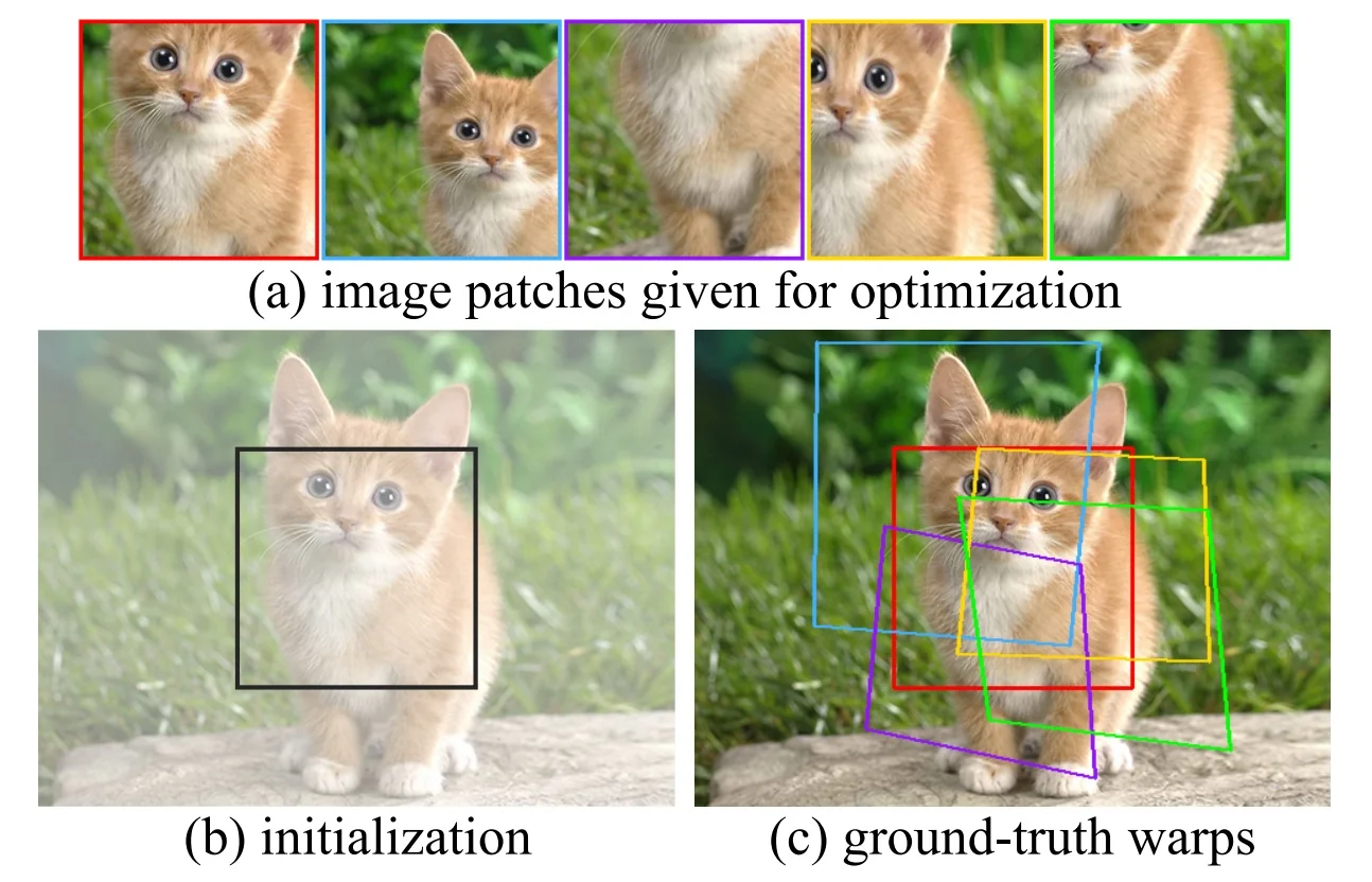
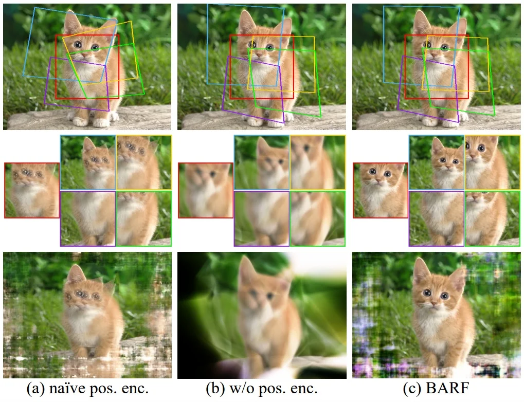
| Positional encoding | \(\mathrm {SL}(3)\) registration error \(\downarrow \) | Patch PSNR (dB) \(\uparrow \) |
| naïve (full) | 0.2949 | 23.41 |
| without | 0.0641 | 24.72 |
| BARF (coarse-to-fine) | 0.0096 | 35.30 |
Synthetic NeRF scenes With synthetic pose noise, BARF realigns cameras and matches the view quality of a pose-supervised NeRF [93].
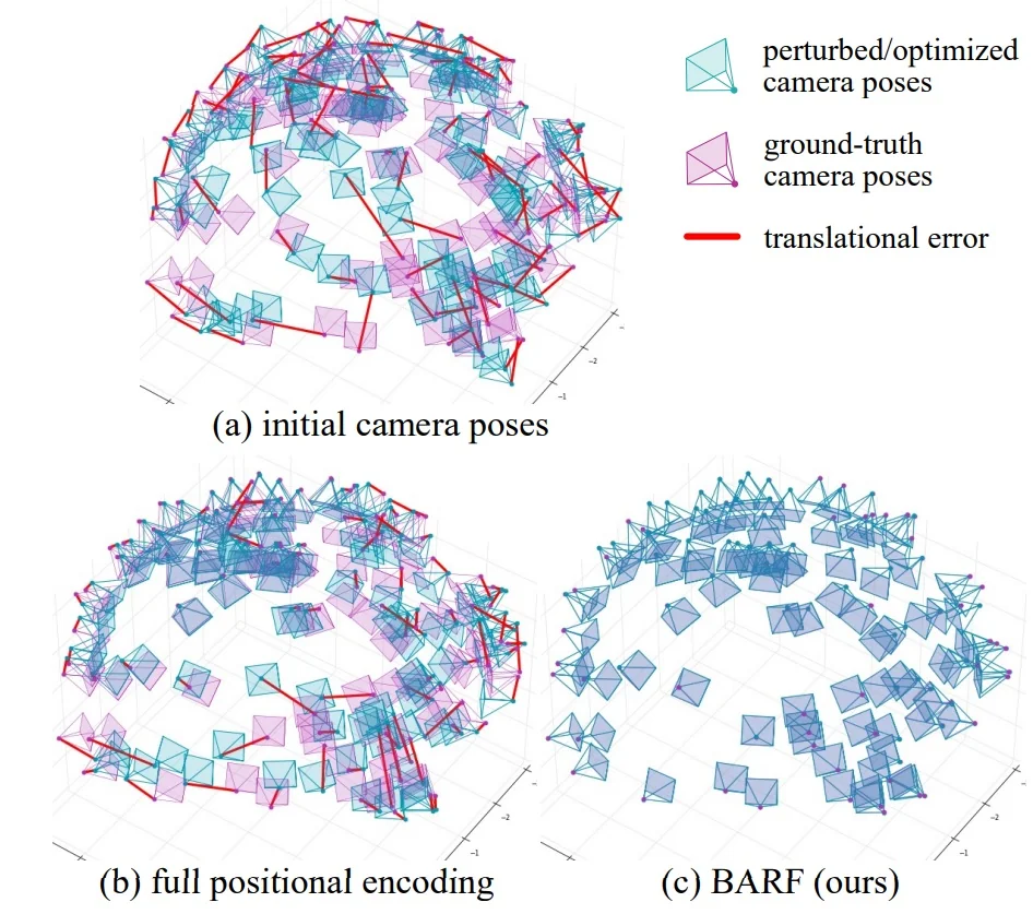
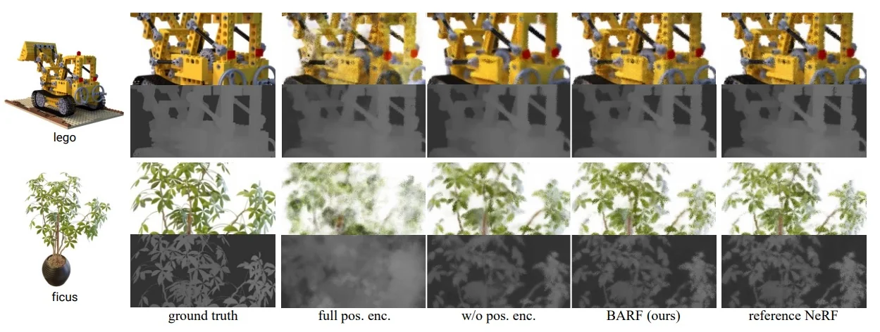
| Scene | PSNR (ref.) | SSIM (ref.) | LPIPS (ref.) | |||||||||||||||
| full | w/o | BARF | full | w/o | BARF | full | w/o | BARF | full | w/o | BARF | full | w/o | BARF | ||||
| Chair | 7.186 | 0.110 | 0.096 | 16.638 | 0.555 | 0.428 | 19.02 | 30.22 | 31.16 | 31.91 | 0.804 | 0.942 | 0.954 | 0.961 | 0.223 | 0.065 | 0.044 | 0.036 |
| Drums | 3.208 | 0.057 | 0.043 | 3.222 | 0.255 | 0.225 | 20.83 | 23.56 | 23.91 | 23.96 | 0.840 | 0.893 | 0.900 | 0.902 | 0.166 | 0.116 | 0.099 | 0.095 |
| Ficus | 9.368 | 0.095 | 0.085 | 10.135 | 0.430 | 0.474 | 19.75 | 25.58 | 26.26 | 26.68 | 0.836 | 0.922 | 0.934 | 0.941 | 0.182 | 0.070 | 0.058 | 0.051 |
| Hotdog | 3.290 | 0.225 | 0.248 | 6.344 | 1.122 | 1.308 | 28.15 | 34.00 | 34.54 | 34.91 | 0.923 | 0.967 | 0.970 | 0.973 | 0.083 | 0.040 | 0.032 | 0.032 |
| Lego | 3.252 | 0.108 | 0.082 | 4.841 | 0.391 | 0.291 | 24.23 | 26.37 | 28.33 | 29.28 | 0.876 | 0.898 | 0.927 | 0.942 | 0.102 | 0.112 | 0.050 | 0.037 |
| Materials | 6.971 | 0.845 | 1.188 | 2.287 | 0.678 | 0.422 | 22.45 | 26.86 | 27.84 | 28.92 | 0.891 | 0.905 | 0.940 | 0.944 | 0.249 | 0.068 | 0.045 | 0.041 |
| Mic | 10.554 | 0.081 | 0.071 | 22.724 | 0.356 | 0.301 | 15.10 | 19.93 | 21.18 | 31.98 | 0.788 | 0.968 | 0.971 | 0.971 | 0.334 | 0.050 | 0.048 | 0.044 |
| Ship | 5.506 | 0.095 | 0.075 | 7.232 | 0.354 | 0.326 | 22.12 | 26.78 | 27.50 | 28.00 | 0.755 | 0.833 | 0.849 | 0.858 | 0.255 | 0.175 | 0.132 | 0.118 |
| Mean | 6.167 | 0.202 | 0.193 | 11.303 | 0.768 | 0.756 | 22.12 | 26.78 | 27.50 | 29.40 | 0.821 | 0.917 | 0.930 | 0.936 | 0.205 | 0.087 | 0.065 | 0.057 |
Real LLFF scenes with unknown poses BARF localizes from identity initialization and achieves synthesis quality comparable to a reference NeRF trained with SfM poses [93].
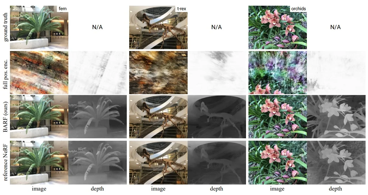
| Scene | Rotation (\(^\circ \))\(\downarrow \) | Translation\(\downarrow \) | PSNR\(\uparrow \) | PSNR (ref.) | SSIM\(\uparrow \) | SSIM (ref.) | LPIPS\(\downarrow \) | LPIPS (ref.) | |||||
| full | BARF | full | BARF | full | BARF | full | BARF | full | BARF | ||||
| Fern | 74.452 | 0.191 | 30.167 | 0.192 | 9.81 | 23.79 | 23.72 | 0.187 | 0.710 | 0.733 | 0.853 | 0.311 | 0.262 |
| Flower | 2.525 | 0.251 | 2.635 | 0.224 | 17.08 | 23.37 | 23.24 | 0.344 | 0.698 | 0.668 | 0.490 | 0.211 | 0.244 |
| Fortress | 75.094 | 0.479 | 33.231 | 0.364 | 12.15 | 29.08 | 25.97 | 0.270 | 0.823 | 0.786 | 0.807 | 0.132 | 0.185 |
| Horns | 58.764 | 0.304 | 32.664 | 0.222 | 8.89 | 22.78 | 20.35 | 0.158 | 0.727 | 0.624 | 0.805 | 0.298 | 0.421 |
| Leaves | 88.091 | 1.272 | 13.540 | 0.249 | 9.64 | 18.78 | 15.33 | 0.067 | 0.537 | 0.306 | 0.782 | 0.353 | 0.526 |
| Orchids | 37.104 | 0.627 | 20.312 | 0.404 | 9.42 | 19.45 | 17.34 | 0.085 | 0.574 | 0.518 | 0.806 | 0.291 | 0.307 |
| Room | 173.811 | 0.320 | 66.922 | 0.270 | 10.78 | 31.95 | 32.48 | 0.278 | 0.940 | 0.948 | 0.871 | 0.099 | 0.083 |
| T-rex | 166.231 | 1.138 | 53.309 | 0.720 | 10.48 | 22.55 | 22.12 | 0.158 | 0.767 | 0.739 | 0.885 | 0.206 | 0.244 |
| Mean | 84.509 | 0.573 | 31.598 | 0.331 | 11.03 | 23.97 | 22.56 | 0.193 | 0.722 | 0.665 | 0.787 | 0.238 | 0.283 |
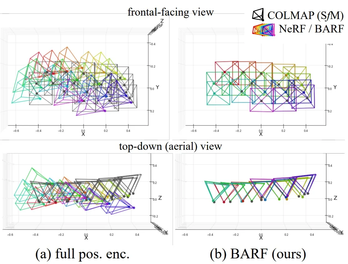
Limitations and future work
- Schedule sensitivity The coarse\(\!\rightarrow \!\)fine bandwidth schedule (\(\alpha (t)\), window \(w_k\)) is hand-set; poor schedules can under/over-regularize early registration and shrink the convergence basin.
- Compute and sampling Jointly optimizing poses and a volumetric field requires dense per-ray sampling and long training, so runtime scales with samples per ray and number of images.
- Scene/model assumptions The formulation assumes static scenes, photometric consistency, and known intrinsics; motion blur, rolling shutter, illumination/exposure shifts, and unknown intrinsics are out of scope.
Follow-ups addressing BARF’s limitations
- Pose robustness with sparse/noisy inputs SPARF augments BARF’s photometric objective with multi-view feature correspondences to jointly refine NeRF and poses from very few, noisy views, improving pose stability when geometric signal is weak [97].
- Pose-free initialization NoPe-NeRF removes the need for pose priors by jointly recovering camera poses and the field from raw images, expanding BARF’s setting to completely unknown extrinsics [98].
- Photometric violations: motion blur BAD-NeRF handles significant motion blur while bundle-adjusting, coupling a deblurring model with pose refinement so that residuals remain informative for registration under real camera shake [99].
- Generalization and efficiency DBARF marries BARF-style bundle adjustment with a generalizable NeRF backbone, improving data-efficiency and robustness across scenes while still refining poses end-to-end [100].
Enrichment 23.11.2: NeRF-W: NeRF for Unconstrained Photo Collections
Motivation
Vanilla NeRF [37] assumes a static, photometrically consistent scene in which geometry, reflectance, and illumination are constant across views. In-the-wild photo collections such as Phototourism [101] break these assumptions due to:
- Substantial photometric shifts (time of day, weather, exposure/white balance, post-processing).
- Transient occluders (people, vehicles, scaffolding).
which, when trained naively, lead NeRF to produce colored fog, ghosting, and biased geometry.
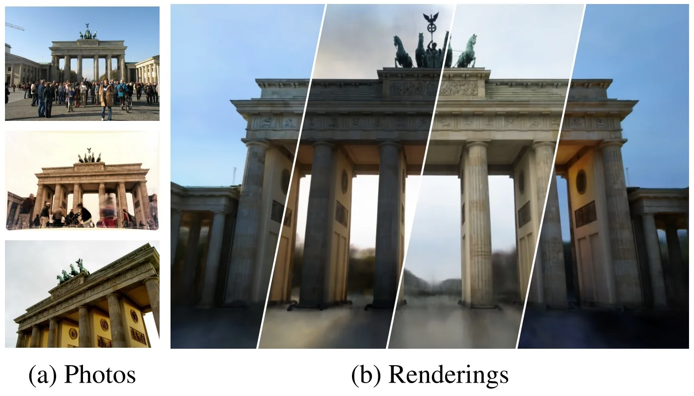
NeRF-W at a glance NeRF-W [94] extends NeRF to Internet photo collections by keeping a single, shared static geometry and routing nuisances into two learned, image-specific factors. Before diving into equations, it helps to fix the data flow and what each part sees and produces:
- Inputs and data flow. Each pixel in image \(I_i\) defines a calibrated ray with world-space samples \(\mathbf {x}\) and a viewing direction \(\mathbf {d}\). The model consumes: position encodings of \(\mathbf {x}\) for geometry, a directional encoding of \(\mathbf {d}\) for view dependence, and two small per-image codes \(\ell ^{(a)}_i\) (appearance) and \(\ell ^{(\tau )}_i\) (transient). Geometry is predicted without any image-specific code; color may depend on both \(\mathbf {d}\) and \(\ell ^{(a)}_i\).
-
Trunk and static field. A NeRF-style trunk maps the position-encoded 3D sample \(\mathbf {x}\) to a static volume density \(\sigma (\mathbf {x})\) and a learned feature vector \(\mathbf {z}(\mathbf {x})\). These features summarize local scene properties beyond coordinates (e.g., geometry/material cues) and are passed to lightweight heads, while \(\sigma (\mathbf {x})\) is computed without any image-specific latent so that one shared geometry is enforced across all images.
- Appearance embedding \(\ell ^{(a)}_i\) and static color head. Each training image \(I_i\) carries a low-dimensional appearance code \(\ell ^{(a)}_i\) that enters only the color branch. The static color head takes the geometric features extracted from the basic geometry network, \(\mathbf {z}(\mathbf {x})\), a directional encoding of \(\mathbf {d}\), and \(\ell ^{(a)}_i\) to produce RGB radiance \(\mathbf {c}_i(\mathbf {x},\mathbf {d})\). Intuition: exposure, white balance, tone mapping, and illumination differences are absorbed by \(\ell ^{(a)}_i\), allowing color to adapt while geometry stays fixed.
- Transient embedding \(\ell ^{(\tau )}_i\) and transient head. A second per-image code \(\ell ^{(\tau )}_i\) drives a transient head that, from \(\mathbf {z}(\mathbf {x})\), predicts an image-dependent density \(\sigma ^{(\tau )}_i(\mathbf {x})\), a transient color \(\mathbf {c}^{(\tau )}_i(\mathbf {x})\), and a per-sample uncertainty signal used during training. Intuition: content that appears only in some photos (people, cars, flags, scaffolding) is explained by this per-image layer instead of corrupting the shared static scene.
- Compositing and learning signal. Along each ray, static and transient opacities jointly control transmittance, and their colors are alpha-composited into a single prediction that is compared to the observed RGB under a Gaussian negative log-likelihood. The rendered per-ray uncertainty down-weights unreliable pixels, and an \(\ell _1\) sparsity prior discourages overuse of the transient density. Intuition: persistent structure must be explained by the static field; ephemeral phenomena are explained sparingly by the transient field; photometric shifts are handled by \(\ell ^{(a)}_i\).
- Inference-time behavior. For novel-view synthesis without a reference image, the transient path is disabled and only the static field is rendered to produce clean, temporally stable views, while the appearance can be controlled by fixing, averaging, or interpolating \(\ell ^{(a)}\) of the scene training images. For a held-out photo, a small \(\ell ^{(a)}\) can be optimized on a subset of its pixels to match its look, with geometry remaining shared because the static \(\sigma (\cdot )\) never depends on \(\ell ^{(a)}\).
Method: Formulation and Derivation
Rendering operator Let a calibrated ray be \(\mathbf {r}(t)=\mathbf {o}+t\,\mathbf {d}\), \(t\in [t_n,t_f]\), with samples \(t_1,\ldots ,t_K\) and steps \(\delta _k=t_{k+1}-t_k\). The discrete volume–rendering operator is \begin {equation} \label {eq:nerfw_R} R(\mathbf {r},\,f,\,\sigma ) \;=\; \sum _{k=1}^{K} T(t_k)\;\alpha \!\big (\sigma (t_k)\,\delta _k\big )\;f(t_k), \qquad \alpha (x)=1-e^{-x}. \end {equation} Here \(T(t_k)=\prod _{k'=1}^{k-1}\exp (-\sigma (t_{k'})\,\delta _{k'})=\exp (-\sum _{k'=1}^{k-1}\sigma (t_{k'})\,\delta _{k'})\) is the cumulative transmittance to the start of slab \(k\), and \(\alpha (\sigma (t_k)\delta _k)=1-\exp (-\sigma (t_k)\delta _k)\) is the per-interval opacity, i.e., the probability the first interaction happens inside slab \(k\) given survival to its entrance.
What \(f\) is in practice and how NeRF-W instantiates \(R\) The operator \(R\) is a generic “first-hit expectation” that composites a per-sample quantity \(f(t)\) under the same probabilistic survival/termination process. NeRF-W uses this operator in two concrete ways: to mix colors from a shared static field and an image-dependent transient field, and to render a per-ray uncertainty that only affects the training loss.
- Single-field baseline (orientation). With one density \(\sigma (\mathbf {x})\) and one per-sample RGB \(\mathbf {c}(\mathbf {x},\mathbf {d})\), taking \(f=\mathbf {c}\) yields the expected color \(R(\mathbf {r},\mathbf {c},\sigma )\), as in vanilla NeRF’s emission–absorption model.
- Two-field color in NeRF-W. NeRF-W adds an image-dependent transient field with density \(\sigma ^{(\tau )}_i\) and color \(\mathbf {c}^{(\tau )}_i\) alongside the shared static field \((\sigma ,\mathbf {c}_i)\). During training, both densities attenuate the ray, so survival uses the joint density, \[ T_i(t_k)\;=\;\exp \!\Big (-\sum _{k'<k}\big [\sigma (t_{k'})+\sigma ^{(\tau )}_i(t_{k'})\big ]\delta _{k'}\Big ). \] The expected color is then the sum of two contributions—one from each field—weighted by their own opacities: \begin {equation} \label {eq:nerfw_composite_color_recap} \hat {\mathbf {C}}_i(\mathbf {r}) \;=\; \sum _{k=1}^{K} T_i(t_k)\Big ( \alpha (\sigma (t_k)\delta _k)\,\mathbf {c}_i(t_k) \;+\; \alpha (\sigma ^{(\tau )}_i(t_k)\delta _k)\,\mathbf {c}^{(\tau )}_i(t_k) \Big ). \end {equation} Intuition: Persistent structure is explained by the appearance-conditioned static color, while image-specific occluders are explained by the transient color; because both densities enter survival, they compete to explain where the first interaction lies.
- Rendered per-ray uncertainty (definition and why transient-only). The transient head, conditioned on the image-specific code \(\ell ^{(\tau )}_i\), outputs an unconstrained value \(\tilde {\beta }_i(t)\) per sample, which we map to a nonnegative scale with a shifted softplus \[ \beta _i(t)\;=\;\beta _{\min }\;+\;\log \!\big (1+\exp (\tilde {\beta }_i(t))\big ), \] where \(\beta _{\min }>0\) avoids zero-variance and prevents the optimizer from entirely ignoring any ray. We then render a ray-wise uncertainty (standard deviation) by alpha-compositing \(\beta _i(t)\) through the transient opacity: \begin {equation} \label {eq:nerfw_rendered_beta} \hat {\beta }_i(\mathbf {r}) \;=\; \sum _{k=1}^{K} T_i(t_k)\,\alpha \!\big (\sigma ^{(\tau )}_i(t_k)\,\delta _k\big )\,\beta _i(t_k), \end {equation} with survival \(T_i\) computed from the joint density \(\sigma +\sigma ^{(\tau )}_i\). Routing via \(\sigma ^{(\tau )}_i\) is intentional: the same transient mechanism that boosts opacity for ephemeral content also gates how much \(\beta _i(t)\) contributes to \(\hat {\beta }_i(\mathbf {r})\). This ties uncertainty exactly to occluders and photometric outliers explained by the transient pathway, rather than diluting it over persistent static structure.
-
How picture-specific content shows up in the transient/uncertainty path.
- What the transient head drives. The transient branch produces a density \(\sigma ^{(\tau )}(t)\), a color \(\mathbf {c}^{(\tau )}(t)\), and an uncertainty carrier \(\beta (t)\). In the color compositor (Eq. (23.44)), \(\sigma ^{(\tau )}\) enters via its opacity \(\alpha (\sigma ^{(\tau )}\delta )\). In the uncertainty compositor (Eq. (23.45)), the same opacity gates how \(\beta (t)\) accumulates into the ray-wise \(\hat {\beta }(\mathbf {r})\).
- When a ray hits ephemeral content. If a ray passes through an occluder or a photometric outlier, training can increase \(\sigma ^{(\tau )}\) on those samples. Two coupled effects follow: (i) \(\alpha (\sigma ^{(\tau )}\delta )\) grows, so \(\mathbf {c}^{(\tau )}\) gets more weight in Eq. (23.44); (ii) the same \(\alpha (\sigma ^{(\tau )}\delta )\) also increases the contribution of \(\beta (t)\) to \(\hat {\beta }(\mathbf {r})\) in Eq. (23.45), making that ray’s supervision softer in the loss.
- When the content is absent. Where no ephemeral content is present, \(\sigma ^{(\tau )}\!\approx \!0\Rightarrow \alpha (\sigma ^{(\tau )}\delta )\!\approx \!0\); both the transient color and the rendered uncertainty vanish, and the ray is supervised normally by the static pathway.
-
Gaussian NLL (training-time reweighting). Notation: dropping image indices. For clarity, when we write \(\mathbf {C}(\mathbf {r})\), \(\hat {\mathbf {C}}(\mathbf {r})\), and \(\hat {\beta }(\mathbf {r})\) without image index, we mean “for the image that \(\mathbf {r}\) comes from”. Concretely, if \(\mathbf {r}\) is sampled from image \(i\), \[ \mathbf {C}(\mathbf {r}) \equiv \mathbf {C}_i(\mathbf {r}),\quad \hat {\mathbf {C}}(\mathbf {r}) \equiv \hat {\mathbf {C}}_i(\mathbf {r})\ \mbox{(Eq.~\eqref {eq:nerfw_composite_color_recap} using }\ell ^{(a)}_i,\ell ^{(\tau )}_i\mbox{)},\quad \hat {\beta }(\mathbf {r}) \equiv \hat {\beta }_i(\mathbf {r})\ \mbox{(Eq.~\eqref {eq:nerfw_rendered_beta})}, \] and in the sparsity term \(\sigma ^{(\tau )}(t_k)\equiv \sigma ^{(\tau )}_i(t_k)\). With this shorthand, we assume isotropic, ray-specific noise, \( \mathbf {C}(\mathbf {r}) \sim \mathcal {N}\!\big (\hat {\mathbf {C}}(\mathbf {r}),\,\hat {\beta }(\mathbf {r})^2\mathbf {I}\big ), \) giving the per-ray NLL (up to a constant) \begin {equation} \label {eq:nerfw_gauss_nll_recap} \begin {aligned} \mathcal {L}(\mathbf {r}) \;=\;& \underbrace {\frac {\big \|\mathbf {C}(\mathbf {r})-\hat {\mathbf {C}}(\mathbf {r})\big \|_2^2}{2\,\hat {\beta }(\mathbf {r})^2}}_{\mbox{(a) data fit: down-weight uncertain rays}} \;+\; \underbrace {\tfrac {1}{2}\log \!\big (\hat {\beta }(\mathbf {r})^2\big )}_{\mbox{(b) variance regularizer}} \;+\; \underbrace {\lambda _u\,\frac {1}{K}\sum _{k=1}^{K}\sigma ^{(\tau )}(t_k)}_{\mbox{(c) transient sparsity}}. \end {aligned} \end {equation}
- (a) Data fit. With \(\mathbf {e}=\mathbf {C}-\hat {\mathbf {C}}\), the residual is scaled by \(1/\hat {\beta }^2\): larger predicted uncertainty \(\Rightarrow \) the ray pays less in the loss and contributes weaker gradients. Because \(\hat {\beta }\) is composited through transient opacity (Eq. (23.45)), this down-weighting targets rays affected by transient phenomena.
- (b) Variance regularizer. The \(\tfrac {1}{2}\log \hat {\beta }^2\) term is the Gaussian normalizer; it prevents the trivial escape \(\hat {\beta }\!\to \!\infty \) and calibrates the learned scale. Minimizing (a)+(b) w.r.t. \(\hat {\beta }^2\) gives \(\hat {\beta }^2=\|\mathbf {e}\|^2\): intuitively, the model is nudged to predict a per-ray variance commensurate with that ray’s squared error—big errors (noisy/hard rays) push \(\hat {\beta }\) up; small errors pull it down. This keeps \(\hat {\beta }\) neither exploding (penalized by \(\log \)) nor collapsing to zero (penalized by the data term).
- (c) Transient sparsity. The \(\ell _1\)-style penalty on nonnegative \(\sigma ^{(\tau )}\) discourages using the transient density to explain persistent structure, preserving a clean static reconstruction.
Training vs. inference. This NLL is used only during training to make supervision robust (via \(\hat {\beta }\)) and to keep transients sparse. At inference, the transient/uncertainty branches are disabled and we render only with \(f=\mathbf {c}\) from the static field, yielding clean, temporally stable views. The dataset-level objective simply sums \(\mathcal {L}(\mathbf {r})\) over all sampled training rays (equivalently \(\sum _i\sum _{\mathbf {r}\in \mathcal {R}_i}\mathcal {L}_i(\mathbf {r})\)).
- Sparse or weak supervision. Regions that are rarely seen, far from cameras, or only observed at oblique angles (e.g., large ground/sky areas) are poorly constrained and often reconstruct with localized blur. The model has too little multi-view evidence to pin down both geometry and appearance (examples in Fig. 23.98).
- Pose/camera errors from SfM. NeRF-W assumes accurate COLMAP poses/intrinsics. Bad estimates introduce inconsistent rays, which the model cannot reconcile, leading to blur/ghosting or wrong structure in affected regions; see discussion in [431].
- Appearance outside the training manifold. The per-image appearance code captures global photometric effects, but extreme illumination/exposure shifts or strong non-Lambertian effects may not be representable, yielding color mismatches even when geometry is correct.
- Imperfect transient separation. Without labels, the transient branch can under/over-explain clutter: some truly static details may be treated as transient (causing holes/softening), or transient residue can remain as faint “fog”.
- (i)
- Joint camera / radiance-field optimization with photometric calibration. Optimizing poses, intrinsics, exposure, and the field together (a neural analogue of bundle adjustment) could correct SfM drift and harmonize brightness/white balance across views, reducing blur and ghosting.
- (ii)
- Stronger disentanglement of illumination vs. exposure/white balance. Factorizing the appearance code into physically meaningful components would enable finer control (e.g., change lighting without altering exposure) and reduce leakage of photometric variation into geometry.
- (iii)
- Learned priors for transient segmentation and temporal consistency. Incorporating priors (e.g., semantic or motion cues) could make the static/transient split more reliable and stabilize renderings across viewpoints, further limiting colored-fog artifacts.
- (iv)
- Scaling to very sparse, long-tail photo collections with better uncertainty calibration. Improving the calibration of per-ray uncertainty (so predicted variances match actual errors) would help the model down-weight unreliable rays more appropriately, making reconstructions more accurate when data are scarce or noisy.
- Source selection: choose a small working set of nearby views for the target camera.
- Geometric proxy: estimate coarse geometry (e.g., SfM/colmap depths, plane-sweep volumes, or multi-plane images) to relate target pixels to source pixels/features.
- Reprojection/warping: use camera intrinsics/extrinsics to warp source evidence (pixels or learned features) toward the target viewpoint.
- Blending & visibility: combine warped evidence with view-dependent weights (heuristic or learned). Errors in proxy geometry or weighting often cause ghosting near occlusions and thin structures.
- Stage 1 — View selection & feature extraction (per selected source view, once). Select \(N\) neighboring source images whose cameras are close to the target pose, whose headings are similar to \(\mathbf {d}\), and whose frusta overlap the target frustum. Each selected image is passed once through a shared encoder–decoder CNN to produce a dense 2D feature map (at reduced resolution). Every pixel of this map encodes a local descriptor mixing appearance and coarse geometric cues (e.g., texture, edges, occlusion hints from context). These learned features are later sampled (via projection) at arbitrary 3D queries to provide per-view evidence about what the scene looks like from that camera. We cache, for each view \(i\), its RGB image, its feature map, and its viewing direction \(\mathbf {d}_i\) so they can be reused for all target pixels/rays.
-
Stage 2 — Per-ray volumetric prediction (uses all \(N\) views at each sampled 3D point). For each target pixel, cast a ray and sample \(M\) points \(\{\mathbf {x}_k\}_{k=1}^{M}\) (near\(\rightarrow \)far). At each sample \(\mathbf {x}_k\) we use all selected views:
- Multi-view gathering. Project \(\mathbf {x}_k\) into each source view \(i\) with the known cameras; bilinearly read the view’s RGB \(\mathbf {C}_i\) and feature vector \(\mathbf {f}_i\) at the projected coordinates (invalid/out-of-frustum projections are skipped or downweighted). Form the relative viewing direction \(\Delta \mathbf {d}_i=\mathbf {d}-\mathbf {d}_i\) (or an angular encoding).
- Color via learned blending. A small shared MLP takes \([\mathbf {f}_i,\ \Delta \mathbf {d}_i]\) and outputs a blending logit \(\alpha _i\). Convert logits to weights via a softmax \[ w_i^{c}=\frac {\exp (\alpha _i)}{\sum _{j=1}^{N} \exp (\alpha _j)},\qquad \sum _i w_i^{c}=1, \] and compute the sample color as a convex combination \[ \mathbf {c}_k=\sum _{i=1}^{N} w_i^{c}\,\mathbf {C}_i. \] Why view dependence is preserved: \(\mathbf {c}_k\) is a weighted copy of actual source pixels, so specularities and other view-dependent effects present in appropriately aligned views are naturally carried into the synthesized color; \(\Delta \mathbf {d}_i\) steers weights toward sources with similar viewing directions [677].
-
Density via ray-wise reasoning.
- (i) Density feature by multi-view pooling (per sample; permutation-invariant). Using the gathered per-view features \(\{\mathbf {f}_i\}_{i=1}^{N}\) at \(\mathbf {x}_k\), compute global statistics to expose agreement/disagreement across views: \[ \boldsymbol {\mu }=\tfrac {1}{N}\sum _{i=1}^{N}\mathbf {f}_i,\qquad \mathbf {v}=\tfrac {1}{N}\sum _{i=1}^{N}(\mathbf {f}_i-\boldsymbol {\mu })^{\odot 2}. \] For each view \(i\), concatenate local and global cues and pass through a shared PointNet-like MLP: \[ \big [\mathbf {f}_i,\ \boldsymbol {\mu },\ \mathbf {v}\big ]\xrightarrow {\ \mathrm {MLP}_\phi \ }\big (\mathbf {f}'_i,\ s_i\big ), \] yielding a multi-view–aware feature \(\mathbf {f}'_i\) and a reliability score \(s_i\). Normalize scores into visibility-aware weights \[ w_i=\frac {\exp (s_i)}{\sum _{j=1}^{N}\exp (s_j)}, \] then form weighted first- and second-order statistics and map them to a compact density feature: \[ \boldsymbol {\mu }_w=\sum _{i=1}^{N} w_i\,\mathbf {f}'_i,\qquad \mathbf {v}_w=\sum _{i=1}^{N} w_i\,(\mathbf {f}'_i-\boldsymbol {\mu }_w)^{\odot 2},\qquad \mathbf {f}_\sigma (\mathbf {x}_k)=\mathrm {MLP}_\psi \!\big ([\boldsymbol {\mu }_w,\ \mathbf {v}_w]\big )\in \mathbb {R}^{d_\sigma }. \] This pooling handles a variable number of views, downweights inconsistent/occluded views, and summarizes multi-view agreement at \(\mathbf {x}_k\) into a fixed-length descriptor predictive of occupancy [677].
- (ii) Ray transformer for coherent densities (per ray). Collect the near-to-far sequence \(\{\mathbf {f}_\sigma (\mathbf {x}_k)\}_{k=1}^{M}\) for one ray and add depth-wise positional encodings \(p_k\) (e.g., sinusoidal in ray parameter \(t_k\)): \[ \mathbf {z}_k=\mathbf {f}_\sigma (\mathbf {x}_k)+p_k,\quad k=1,\dots ,M. \] A lightweight ray transformer (single multi-head self-attention layer) processes \(\{\mathbf {z}_k\}\) so each sample attends to the others along the same ray. Intuitively, strong near-field evidence can suppress spurious far-field candidates, and clusters of consistent samples reinforce surfaces. The attended features \(\{\hat {\mathbf {z}}_k\}\) are passed through a tiny head to obtain nonnegative densities: \[ \sigma _k=\mathrm {MLP}_\rho \!\big (\hat {\mathbf {z}}_k\big ),\qquad k=1,\dots ,M. \]
Figure 23.99: Density and color prediction at a 5D location \((\mathbf {x},\mathbf {d})\) in IBRNet [677]. Per-view features \(\{\mathbf {f}_i\}\) are combined with global statistics (mean/variance) by a PointNet-like MLP to produce multi-view–aware features and visibility-aware weights; weighted pooling yields a compact density feature \(\mathbf {f}_\sigma \). A ray transformer consumes the sequence \(\{\mathbf {f}_\sigma (\mathbf {x}_k)\}\) on a ray (with positional encodings) and outputs coherent densities \(\{\sigma _k\}\). For color, a blending head uses \([\mathbf {f}_i,\Delta \mathbf {d}_i]\) to predict weights that form \(\mathbf {c}_k\) as a weighted average of source colors, preserving view-dependent effects. - Stage 3 — NeRF-style volume rendering & training (per pixel). With \((\mathbf {c}_k,\sigma _k)\) at sorted depths along the ray, let \(\delta _k\) denote the spacing between consecutive samples (e.g., \(\delta _k = t_{k+1}-t_k\) in ray-parameter units). The transmittance to sample \(k\) is \[ T_k=\exp \!\Big (-\sum _{j=1}^{k-1}\sigma _j\,\delta _j\Big ), \] and the rendered pixel color is \[ \tilde {\mathbf {C}}(\mathbf {r})=\sum _{k=1}^{M} T_k\Big (1-e^{-\sigma _k\,\delta _k}\Big )\,\mathbf {c}_k. \] Training follows the familiar coarse/fine hierarchical sampling and an \(\ell _2\) photometric loss on both passes. The renderer is unchanged from NeRF [442]; what differs is how \((\mathbf {c},\sigma )\) are predicted: here they are inferred on-the-fly from the target scene’s images and features, using weights learned across many training scenes [677].
- Per-image encoder–decoder CNN (shared). A U-Net/ResNet34-style encoder–decoder (Instance Normalization as replacement of BatchNorm) processes each selected source image once to produce a dense 2D feature map at reduced resolution (output: \(160\!\times \!120\!\times \!64\)).1 These features are cached and later sampled by projection at arbitrary 3D queries.
-
Per-sample MLP heads (shared across views and rays).
- Color head (blending). Given a projected feature \(\mathbf {f}_i\) from view \(i\) and the relative viewing direction \(\Delta \mathbf {d}_i\), a small MLP outputs a scalar blending logit whose softmax across views yields weights \(\{w_i^c\}\). The sample color is \(\mathbf {c}_k=\sum _i w_i^c \mathbf {C}_i\) (a convex blend of actual source colors), preserving view dependence.
- Density pooling head. For density, a PointNet-like shared MLP maps \([\mathbf {f}_i,\boldsymbol {\mu },\mathbf {v}]\) (local feature with global across-view mean/variance) to a multi-view–aware feature \(\mathbf {f}'_i\) and a reliability score \(s_i\). Softmax-normalized scores provide visibility-aware weights \(w_i\!\propto \!\exp (s_i)\). Weighted mean/variance over \(\{\mathbf {f}'_i\}\) are then mapped by a tiny MLP to a compact density feature \(\mathbf {f}_\sigma (\mathbf {x}_k)\!\in \!\mathbb {R}^{d_\sigma }\) (e.g., \(d_\sigma {=}16\)).
- Ray transformer (single layer, along-ray self-attention). For one ray, the sequence \(\{\mathbf {f}_\sigma (\mathbf {x}_k)\}_{k=1}^{M}\) (with depth-wise positional encodings) is processed by a single multi-head self-attention layer (4 heads). The attended features feed a tiny head to produce nonnegative densities \(\{\sigma _k\}\) jointly for all samples, improving depth ordering and occlusion handling.
- Cameras on the upper hemisphere are subsampled by factors \(\{2,4,6,8,10\}\) to simulate progressively sparser capture.
- Hence, for a given target view, the number of selectable neighbors \(N\) and baselines decrease, reducing parallax and multi-view agreement.
- The rendering pipeline and loss remain unchanged; only the available inputs differ.
- Observed effect of sparsity (Figure 23.101). As source views become sparser, errors grow near thin structures, specular regions, and occlusion boundaries. This is consistent with weaker multi-view consistency and fewer reliable visibility cues.
- Zero-shot robustness. The pretrained (scene-agnostic) model degrades gracefully: despite reduced inputs, the learned fusion recovers large-scale structure and many details, indicating effective cross-scene priors.
-
Procedure.
- Initialize all network parameters from the scene-agnostic pretrained model (shared encoder–decoder CNN, per-sample MLP heads for color and density pooling, and the ray transformer).
- Optimize on the posed images of the target scene using the same NeRF-style objective: coarse/fine hierarchical sampling of ray points and an \(\ell _2\) photometric loss between rendered and ground-truth pixel colors [677].
- Keep the rendering pipeline, view selection (\(N\) neighbors), sampling strategy, and losses unchanged; only the weights are updated. In practice, rays are randomly sampled across training images each iteration, and both coarse and fine branches are trained jointly as in the pretrained model.
-
What is adapted. Fine-tuning specializes the generic, cross-scene priors to the geometry/appearance and camera layout of the specific scene by calibrating:
- Visibility-aware pooling. The PointNet-like density-pooling head refines the reliability scores \(\{s_i\}\) and resulting weights \(\{w_i\}\) so that views inconsistent or occluded at a sample location receive lower influence when forming the compact density feature \(\mathbf {f}_\sigma (\mathbf {x}_k)\).
- Color blending. The color head adjusts how relative viewing directions \(\Delta \mathbf {d}_i\) and per-view features \(\mathbf {f}_i\) are mapped to blending weights \(\{w_i^c\}\), improving reproduction of scene-specific view-dependent effects (e.g., specularities) under the available baselines.
- Along-ray reasoning. The ray transformer adapts its self-attention to the scene’s depth statistics, helping resolve near–far ordering and occlusions more decisively when aggregating \(\{\mathbf {f}_\sigma (\mathbf {x}_k)\}_{k=1}^M\).
- Low-level features. The shared encoder–decoder CNN updates its filters so that the 2D feature maps align with the target scene’s photometric characteristics (exposure, material cues, texture scale), which strengthens the multi-view consistency signal used downstream.
-
Why it helps under sparsity.
- With few and narrowly spaced source views, the generic priors learned across many scenes may be insufficient to disambiguate thin structures and complex occlusions. Fine-tuning reduces this domain gap by aligning the priors to the target scene’s actual pose/appearance distribution.
- Calibrated visibility weights decrease uncertainty in \(\mathbf {f}_\sigma \), steering density toward physically plausible surfaces and away from “black-hole” artifacts.
- Refined color blending emphasizes the most reliable source rays for each 3D sample, improving view-dependent appearance without introducing high-frequency regression artifacts.
- The adapted ray transformer strengthens along-ray suppression of spurious far samples once a nearer surface is explained, yielding cleaner boundaries and fewer floaters.
-
Empirical takeaway (Figure 23.101).
- As input views are made sparser, IBRNet\(_\mbox{ft}\) consistently degrades more gracefully than the zero-shot model: edges remain sharper, thin structures persist longer, and occlusion boundaries are cleaner, while the rendering objective and architecture remain unchanged [677].
- pixelNeRF [762] (CVPR 2021): conditions a NeRF directly on image-aligned features from one/few inputs and regresses color/density. Unlike IBRNet’s explicit color blending and along-ray transformer, pixelNeRF relies on a fully convolutional conditioning pipeline for feed-forward generalization.
- GRF [652] (ICCV 2021; arXiv 2020): learns a general radiance field by projecting pixel features to 3D and aggregating across views (with attention). Compared to IBRNet, GRF eschews pixel copying/blending and focuses on implicit field regression conditioned on inputs.
- MVSNeRF [79] (ICCV 2021): imports plane-sweep cost volumes and 3D CNNs from MVS for geometry-aware aggregation. In contrast to IBRNet’s PointNet-style pooling plus a ray transformer, MVSNeRF leverages explicit multi-plane geometry priors to guide density/color regression and supports fast feed-forward reconstruction with optional per-scene fine-tune.
- NeuRay [392] (CVPR 2022): augments feature aggregation with an explicit, learned per-view visibility field. For each 3D query, the method predicts how visible it is from every source camera and downweights occluded/inconsistent evidence before color/density prediction. Compared to IBRNet’s implicit, score-based pooling, NeuRay disentangles visibility estimation from appearance blending.
- GeoNeRF [278] (CVPR 2022): injects stronger geometry by constructing multi-scale cost volumes (plane-sweep style) and fusing them with a Transformer. This emphasizes epipolar consistency and depth reasoning more explicitly than IBRNet’s PointNet-like pooling, improving few-view robustness and occlusion handling.
- Point-NeRF [736] (CVPR 2022): anchors features on a neural point cloud and renders through point-based volume rendering. In contrast to IBRNet’s pixel-aligned (per-view) feature sampling, Point-NeRF shifts to a scene-adaptive, point-anchored representation that can be efficient and accurate when reliable points are available.
- RegNeRF [466] (CVPR 2022): remains per-scene but targets the same sparse-input failure modes via strong regularization (e.g., unseen-view patch losses, sampling annealing). While not cross-scene like IBRNet, it offers complementary loss/regularization ideas that can inspire priors for generalizable renderers.
- Conditioning mechanism: pixel-aligned sampling (IBRNet) vs. cost-volume aggregation (GeoNeRF) vs. point-anchored features (Point-NeRF).
- Visibility modeling: implicit reliability pooling + along-ray attention (IBRNet) vs. explicit per-view visibility fields (NeuRay) vs. geometry-constrained matching in volumes (GeoNeRF).
- Training regime: cross-scene, feed-forward generalization (IBRNet, NeuRay, often GeoNeRF variants) vs. per-scene but robustly regularized optimization (RegNeRF).
- Trade-offs: stronger geometry priors tend to improve occlusions and thin structures under extreme sparsity, while pixel/feature-conditioned designs often yield higher throughput and simpler deployment across scenes.
- Full The complete PixelNeRF model conditions the radiance field on fine-grained, pixel-aligned image features and includes the NeRF-style viewing direction input \(\mathbf {d}\) to capture view-dependent appearance.
- -- Local Replaces pixel-aligned features with a single global image code. This removes spatially precise conditioning at projected locations \(\pi (\mathbf {x})\), testing whether per-pixel alignment is essential for shape/detail recovery.
- -- Dirs Removes the explicit direction input \(\mathbf {d}\) to test the importance of view-dependent effects (e.g., specularities) under sparse supervision.
- Rendering speed. PixelNeRF inherits NeRF’s slow volumetric rendering, with runtime scaling linearly with the number of input views. This makes interactive applications infeasible.
- Positional encoding scale. The choice of frequency bands in \(\gamma (\cdot )\) and manually tuned ray sampling bounds limit scale invariance. PixelNeRF struggles when scenes deviate strongly in scale or depth range.
- Dataset constraints. Training and evaluation rely on ShapeNet and DTU, which are synthetic or controlled. Generalization to in-the-wild 360\(^\circ \) captures is still limited.
- IBRNet [677] improved multi-view aggregation with attention-based pooling, enhancing generalization across unseen scenes.
- MVSNeRF [79] introduced cost-volume features to better exploit geometric consistency under sparse views.
- PixelNeRF++ and other variants investigated scaling the approach to more complex outdoor or dynamic settings.
- Vision transformers for NeRF priors (e.g., [392, 278]) replaced CNN encoders with transformers for improved visibility reasoning and global context.
- Block-NeRF [623]: Composes geographic “blocks” to model city-scale environments with streaming and modular training.
- Mip-NeRF 360 [28]: Tackles unbounded \(360^\circ \) scenes with integrated positional encoding and anti-aliased cones.
- Nerfies [483]: Learns continuous deformation fields from casual handheld videos for non-rigid, dynamic scenes.
- D-NeRF [502]: Extends NeRF with time as an input for explicit scene dynamics.
- Geographic tiling of the street network into overlapping blocks using priors such as intersection coordinates and segment lengths (from maps or HD-road graphs).
- Per-block training of compact mip-NeRFs (see Enrichment 23.10.5) on geographically filtered images, with appearance embeddings, exposure conditioning, and pose refinement to absorb long-term capture variability.
- Visibility-driven selection of only the few blocks that actually see the current view, using a small visibility network to cull irrelevant blocks.
- Cross-block compositing and appearance alignment to merge rendered images smoothly and reconcile style differences across time, weather, and cameras.
- Geometric continuity: Overlap ensures that street geometry and building façades crossing block boundaries are represented consistently by at least two models, reducing visible seams during rendering.
- Appearance alignment: Because training images are captured under different conditions (day/night, clear/cloudy, varied camera exposure), overlap provides shared pixels where neighboring blocks can align their appearance embeddings. Without overlap, blocks could converge to inconsistent colors or lighting, producing sharp discontinuities.
- 1.
- Geographic initialization: Block origins are selected at intersections or uniformly along long street segments, using map priors such as OpenStreetMap or HD-road graphs.
- 2.
- Coverage definition: Each block is defined as a sphere or radius around the origin, extending most of the way toward neighbors to enforce overlap.
- 3.
- Geographic filtering of training data: Each training image is assigned to blocks based on whether its camera frustum intersects the block’s coverage region. This ensures that each Block-NeRF only sees the data relevant to its intended sub-region.
- 4.
- Independent training: Blocks are trained independently in parallel, producing a modular set of models. This modularity allows retraining only the affected blocks when local changes occur (e.g., construction on one street), rather than reoptimizing the entire city.
- Appearance embeddings (per-image latent codes) absorb day-to-day or seasonal shifts in illumination and weather, ensuring that lighting changes are captured photometrically rather than as spurious geometry.
- Exposure conditioning encodes camera exposure values (e.g., shutter speed \(\times \) gain) with a sinusoidal positional encoding, stabilizing training under brightness fluctuations and enabling interpretable exposure control at inference.
- Pose refinement introduces small, regularized SE(3) offsets per driving segment to correct residual odometry drift, mitigating ghosting and duplication artifacts at block boundaries.
- 1.
- Candidate selection: Gather blocks within radius \(R_{\mbox{select}}\) of the camera center \(c\).
- 2.
- Visibility pruning: For each candidate, probe \(f_v\) at a sparse set of sample points/rays from \(c\) and average predictions. Blocks with low mean visibility are culled. Typically only \(1\)–\(3\) remain, preventing compute waste on blocks that are occluded or irrelevant.
- 3.
- Rendering: Surviving blocks are fully rendered with mip-NeRF ray marching.
- 4.
- Compositing: Per-block images \(\mathbf {I}_i\) are combined with inverse-distance weights, producing a seamless output. Distance-based blending is temporally stable, avoiding flicker in flythroughs.
- 5.
- Appearance alignment: To harmonize across different lighting conditions, \(f_v\) also identifies high-visibility overlap between neighboring blocks. In these regions, adjacent blocks adjust their latent appearance codes so that colors match the reference block, yielding globally consistent appearance (time-of-day, weather, white balance).
- 1.
- Fix a reference block with a chosen appearance code \(\ell ^{\mbox{ref}}\).
- 2.
- For each neighboring block \(j\), use \(f_v\) to identify overlap regions that are simultaneously visible.
- 3.
- Optimize only \(\ell _j\), keeping network weights frozen, to minimize color differences over the shared patch: \[ \min _{\ell _j} \sum _{p \in \mathcal {P}} \big \|\mathbf {I}_{\mbox{ref}}(p;\,\ell ^{\mbox{ref}}) - \mathbf {I}_j(p;\,\ell _j)\big \|^2. \]
- 4.
- Propagate alignment outward across the block graph.
- Dynamic radiance fields for explicitly modeling moving objects.
- Unbounded representations (e.g., NeRF++ [792], mip-NeRF 360 [28]) for sharper distant reconstructions.
- Acceleration techniques such as voxel caching [379, 763] or hash encodings [457] for real-time rendering and faster training.
- Global parameterization. Fitting an unbounded world into a fixed near/far box squeezes very distant geometry into a tiny coordinate range, so equal steps in model space correspond to huge steps in world space at the far field, leaving too few effective intervals for the entire background and causing blur despite intra-interval anti-aliasing [29, 28].
- Sampling geometry. Uniform steps in metric depth \(t\) devote many samples to nearby content (large pixel footprint) but too few to distant content (tiny footprint), which yields aliasing and loss of detail in horizons and skies for fully 360° captures [28].
- Capacity vs. efficiency. Large, real scenes mix extremely near and far structure; making a single mip-NeRF MLP sufficiently large and supervising it at multiple scales is expensive, so capacity is constrained by training cost [29].
- Ambiguity and artifacts. The inverse problem is underconstrained at scale; optimization can explain pixels via semi-transparent blobs (floaters) or by dragging distant matter toward the camera (background collapse). Noise injection and multi-scale supervision help but neither controls how mass is arranged along a ray nor fixes the global parameterization mismatch [442, 29].
- 1.
- Nonlinear scene reparameterization. A smooth contraction maps \(\mathbb {R}^3\) into an isotropic ball of radius \(2\) while leaving the unit ball around the camera unchanged. Preserving the unit ball keeps local metric geometry faithful where pixels are most sensitive (foreground parallax and high-frequency detail). Compressing the exterior into the shell \(1\!\to \!2\) makes “infinity” finite and numerically well-behaved, and the extra radius beyond \(1\) provides dynamic range so far depths do not collapse onto a single boundary. The spherical target avoids axis/corner biases of a cube, treating all directions symmetrically. Paired with disparity-linear spacing along rays, equal steps in the contracted coordinate correspond more closely to equal changes in image footprint at long range, restoring a well-conditioned sampling geometry for unbounded scenes.
- 2.
- Proposal-driven hierarchical sampling. Each camera ray is
divided into contiguous segments (intervals) in a normalized
coordinate \(s\in [0,1]\), yielding a 1D histogram with a nonnegative weight per
interval that reflects its contribution to the pixel after volumetric
compositing. What changes versus mip-NeRF is the division of labor:
rather than repeatedly querying and supervising the same MLP at
multiple scales, MipNeRF360 [28] decouples where to sample from what
to predict. A small proposal MLP is evaluated on a coarse, roughly
uniform partition (in the contracted, disparity-linear coordinate) to
produce a coarse weight profile that guides where the ray should
be refined; the ray is then re-partitioned so intervals concentrate
around the predicted peaks (optionally repeating this proposal step
once more). Only after this final, content-focused partition has been
built is the high-capacity NeRF MLP run—once per ray at a single
stage, namely on the final set of intervals—by querying it at each
final interval to predict densities and colors for the actual rendering.
To make the proposal reliable without adding another image loss,
a lightweight histogram-consistency objective trains the proposal to
cover the support that the NeRF MLP ultimately uses (gradients
flow only into the proposal in this term), ensuring the sampler does
not overlook mass that the renderer needs. In short, mip-NeRF’s
multi-scale rendering is replaced by a cheap sampler (proposal MLP)
plus a single high-fidelity renderer (NeRF MLP), concentrating
expensive computation exactly where it matters most [28].
Why this improves things:
- The proposal amortizes search, so the final intervals rapidly cluster near actual surfaces instead of being wasted in empty space.
- The NeRF MLP avoids redundant coarse-and-fine rendering passes, enabling higher capacity without prohibitive training cost.
- The consistency term keeps proposals conservative (they must cover what NeRF uses), reducing missed surfaces and aliasing in unbounded scenes.
- 3.
- Distortion regularization. Like mip-NeRF, each interval is a conical
frustum approximated by a 3D Gaussian and is anti-aliased within the
interval via integrated positional encoding; what those methods do not
control is how the total weight is distributed across intervals along the ray.
In unbounded scenes this longitudinal ambiguity is a major failure mode:
the optimization can explain a pixel by spreading small weights over
many separated intervals (yielding semi-transparent floaters), or by
shifting mass into near intervals to shorten optical paths (background
collapse). MipNeRF360 [28] adds a distortion loss that penalizes
spread of the per-ray weight histogram in the normalized coordinate \(s\)
(via pairwise distances between interval midpoints plus a width
term).
High level: the loss softly prefers compact, near-unimodal allocations across intervals when consistent with the images, steering the solution toward “a surface here” rather than many faint lobes along the line of sight. This complements the within-interval anti-aliasing (unchanged) and, together with the proposal-guided sampling and contraction, reduces floaters, discourages background collapse, and yields sharper, more plausible geometry in 360° environments [28].
- Background blur. In Euclidean \(t\), a fixed number of intervals must span an enormous depth range, so each far interval covers a huge swath of world space; its Gaussian/IPE averages many distinct background colors, appearing blurry. After contraction paired with disparity-linear spacing (explained below), the far field occupies a finite, uniformly coverable band in the warped coordinate. Intervals become approximately equal-sized in the contracted radius, so the background is represented by many small, distinct bins rather than a few massive ones. Less averaging \(\Rightarrow \) sharper backgrounds.
- Background collapse. With poor far-field resolution, optimization can “cheat” by pulling density toward the camera: shorter paths can reproduce colors with fewer samples, so mass drifts forward. In the contracted domain, moving density from the far shell toward the near region causes large displacements in the warped coordinate (and hence stronger reconstruction penalties), while the far band itself now has sufficient resolution to place density where images demand it. The optimization no longer gains an easy advantage by collapsing the background forward.
- Matches image sensitivity. In a pinhole camera, a fronto-parallel patch at depth \(z\) projects with scale \(\propto 1/z\); small image changes are roughly proportional to changes in disparity \(d=1/z\) (since \(\,\partial \,\)image\(/\partial d\) stays more nearly depth-invariant than \(\,\partial \,\)image\(/\partial z\)). Uniform steps in \(s\) therefore allocate samples in proportion to perceptual/photometric change along the ray, especially at long range, improving coverage of sky and distant objects.
- Pairs with contraction. For a camera at the origin, the contraction radius along a ray is \(r'(t)=2-\tfrac {1}{t}\). Uniform steps in \(s\) with \(g(t)=1/t\) (i.e., uniform disparity) produce approximately uniform steps in \(r'\) across the outer shell. Thus, a fixed sample budget yields near-uniform spatial coverage in the warped domain, which is the domain where features are computed.
- Numerical stability and consistency. Normalizing every ray to \(s\!\in [0,1]\) makes histograms, losses (proposal consistency, distortion), and resampling ray-agnostic: bin sizes, gradients, and learning rates do not depend on unknown scene scales or ad-hoc near/far ranges. The mapping in Eq. (23.54) recovers \(t\) only where metric distances are required (e.g., transmittance factors), avoiding depth-scale–dependent conditioning in the rest of the pipeline.
- Coarse partition and proposal histogram. Start by partitioning \(s\in [0,1]\) into contiguous bins with endpoints \(\hat {t}=\{\hat {t}_0,\ldots ,\hat {t}_{M}\}\) (paper notation uses \(t\) for bin edges; here \(\hat {t}\) indicates the proposal partition; \(t\)/\(\hat {t}\) can be read as any monotone ray coordinate, e.g., \(s\)). Evaluate the proposal MLP at these bins and convert predicted densities to a proposal weight histogram \((\hat {t},\hat {w})\) using the standard volumetric compositing weights (cf. NeRF/mip-NeRF; see Eq. (23.67) in the previous subsection).
- Importance resampling. Treat \(\hat {w}\) as a distribution over the ray and resample to form a finer partition that concentrates bins where \(\hat {w}\) is large (near likely surfaces). The paper uses one or two proposal stages, each producing its own \((\hat {t},\hat {w})\) and a refined partition.
- Final rendering pass. Only after the final, content-focused partition is constructed, evaluate the high-capacity NeRF MLP once per ray at a single stage: query it at each final interval to predict density and color, and composite to the pixel. This avoids redundant coarse-and-fine renderings of the same ray while still guiding samples to informative regions.
- Coarse may over-cover, must not under-cover. A coarse proposal can safely spread mass broadly—resampling will zoom into its peaks—but it must not omit mass where the final pass concentrates; otherwise, that region could never be discovered. The bound in Eq. (23.55) encodes exactly this asymmetry by demanding that every final-bin weight be “explainable” by overlapping proposal mass.
- Independent of bin layout and size. Because the bound sums proposal mass over overlaps, it tolerates different bin counts and widths and does not assume aligned edges. Merging or splitting proposal bins while conserving mass does not change whether a region is covered.
- Loss roles at a glance. The NeRF MLP optimizes image reconstruction (and, later, distortion) on the final partition, while the proposal MLP optimizes \(\mathcal {L}_{\mathrm {prop}}\) to learn a conservative cover around NeRF’s weight distribution. This division of labor lets the small network amortize “where to look” and the large network focus capacity on “what to predict”, improving both speed and accuracy in unbounded scenes.
- Annealing. Before drawing fine samples from \(\hat {w}\), raise weights with a Schlick-biased schedule over step \(n\!\in [0,N]\), \[ \hat {w}_n \propto \hat {w}^{\frac {b\,n/N}{(b-1)\,n/N+1}},\quad b=10. \] Early in training, this flattens the distribution (exploration across the ray); as training proceeds, it sharpens back to \(\hat {w}\) (exploitation near predicted surfaces). This avoids premature lock-in to spurious peaks.
- Dilation. Convert the histogram to a density \(\hat {p}_i=\hat {w}_i/(\hat {t}_{i+1}-\hat {t}_i)\), replace \(\hat {p}\) by a local maximum over \(s\pm \epsilon _k\) with \[ \epsilon _k=\frac {a}{\prod _{k'=1}^{k-1} n_{k'}} + b,\quad a=0.5,\; b=0.0025, \] where \(n_k\) is the number of fine samples drawn at proposal level \(k\), then integrate back and renormalize. This creates a small, scale-aware safety margin around peaks so that minor pose/view changes do not cause the proposal to miss a thin surface (reduces rotational aliasing).
- Midpoint resampling. Draw \(n{+}1\) sorted samples from the coarse histogram and use midpoints of adjacent samples (including reflected endpoints) as the new bin edges. Using raw samples as edges erodes peaks and creates irregular gaps; midpoints preserve modes and yield more even, low-alias partitions.
- Proposal guidance. Removing the proposal MLP stages and sampling only from the final network leads to degraded quality and visible floaters, confirming the necessity of the histogram-consistency training.
- Distortion loss. Disabling \(\mathcal {L}_{\mathrm {dist}}\) produces fragmented weight distributions along rays, resulting in floaters and background collapse. Compared to density-noise injection, \(\mathcal {L}_{\mathrm {dist}}\) yields superior suppression of artifacts without sacrificing fine detail.
- IPE vs. standard PE. Replacing integrated positional encoding with ordinary positional encoding reduces performance in unbounded scenes, especially where anti-aliasing is critical. Off-axis IPE further improves handling of anisotropic footprints.
- Single vs. multi-proposal. Using two proposal stages instead of one refines the sampling distribution more reliably, especially in challenging rays with both near and far content.
- Training cost. The multi-stage proposal guidance and large NeRF MLP make training computationally demanding compared to lightweight or grid-based alternatives.
- Rendering speed. At test time, inference is slower than real-time systems such as PlenOctrees or Instant-NGP, since MipNeRF360 still relies on MLP queries along rays.
- Over-regularization. In some cases, the distortion loss can oversimplify weight distributions, slightly reducing fine detail in favor of compactness.
- Scene priors. While contraction handles unbounded domains, scenes with extreme depth ranges or severe occlusion patterns may still exhibit artifacts or require many proposal samples to converge.
- Temporal consistency. Consider the tip of a moving finger: without alignment, the network must memorize its material properties at every position along its trajectory. With the canonical anchor, the finger tip maps to a single coordinate, preserving sharp detail.
- Separation of dynamics from statics. Static background points (e.g., walls) map trivially to themselves, while dynamic objects (e.g., a bouncing ball) are displaced by the learned deformation. The canonical network can thus specialize in view-dependent appearance, while motion complexity is isolated in the deformation field.
- a deformation network \(\Psi _t\), which aligns points observed at time \(t\) with a canonical space,
- a canonical network \(\Psi _x\), which predicts density and radiance in the canonical configuration.
- NeRF [442], which assumes static scenes and therefore cannot handle motion.
- T-NeRF, a temporal baseline that directly regresses \[ (\mathbf {x}, \mathbf {d}, t) \mapsto (\mathbf {c}, \sigma ), \] without using a canonical space or deformation field. T-NeRF highlights the shortcomings of naive temporal modeling: while it can capture coarse changes over time, it treats the same physical point at different instants as unrelated, leading to blurred details and inconsistent geometry. Importantly, T-NeRF is not D-NeRF without curriculum learning, but rather the simplest 6D extension of NeRF used as a baseline.
- NeRF [442], which assumes static scenes.
- T-NeRF, a 6D extension that directly regresses \((\mathbf {x}, \mathbf {d}, t) \mapsto (\mathbf {c}, \sigma )\) without canonical warping.
- Training cost. Like NeRF, D-NeRF relies on volumetric rendering that requires querying MLPs hundreds of times per ray. The addition of a deformation network compounds this cost, making training slow and memory-intensive (on the order of days on a single GPU).
- Synthetic focus. D-NeRF’s evaluation is confined to clean, synthetic sequences with known camera parameters and dense coverage. Its performance on real-world captures—with noise, sparse viewpoints, and imperfect calibration—remains unexplored.
- Deformation capacity. The deformation field is assumed to be smooth and bijective, mapping each observation into the canonical space. While effective for simple motions, this assumption struggles with complex dynamics such as large occlusions, self-contact, or true topological changes (e.g., an object splitting or a mouth opening/closing).
- Canonical anchoring. D-NeRF typically fixes the canonical frame at \(t=0\), which is arbitrary. If the first frame is occluded or atypical, this choice can bias correspondences across time and destabilize optimization.
- From synthetic to real-world capture. Extending canonical–deformation frameworks to unconstrained mobile videos requires handling photometric inconsistency, calibration errors, and drifting backgrounds.
- From weak to stronger priors. Beyond smoothness assumptions, deformation fields benefit from geometric regularizers that bias them toward locally rigid or cycle-consistent warps, preventing collapse into degenerate solutions.
- From arbitrary to flexible canonicalization. Conditioning deformations purely on time anchors the canonical space too rigidly; more adaptive conditioning strategies are needed to capture variations across diverse observations.
- From expensive to efficient training. Reducing the heavy computational footprint of dynamic NeRFs—without sacrificing fidelity—remains a central challenge, inspiring later work on acceleration and hybrid representations.
- Decoupling from absolute time: Conditioning deformations on a per-image latent code \(\omega _i\) instead of the scalar time index \(t\) removes an arbitrary temporal anchor (e.g., \(t{=}0\)) and improves flexibility for casually captured sequences with irregular motion
- Locally rigid motion modeling: Using dense \(\mathrm {SE}(3)\) transforms allows compact, coherent representation of rotations and translations across space, addressing ambiguity that displacement fields face when mimicking rotation via spatially varying translations
- Bias toward plausible deformations: Elastic regularization on the deformation Jacobian and a c2f frequency-annealing schedule guide optimization away from degenerate warps in under-constrained settings
- Removal of arbitrary anchoring: Deformations are no longer tied to \(t{=}0\), avoiding bias toward whichever frame was chosen as the reference.
- Observation-based indexing: States are referenced by observation identity rather than clock time, allowing out-of-order or irregular captures to be modeled consistently.
- Interpolatable state space: The latent deformation codes live in a continuous space, so smooth synthesis of intermediate states is possible by interpolating between codes.
- Novel view of a training frame. Suppose we want to see frame \(i\) (same body pose, same facial expression, etc.) but from a new camera angle. We simply reuse its learned codes \((\omega _i,\psi _i)\). Rays are cast from the new camera, warped into canonical space by \(T(\mathbf {x},\omega _i)\), and rendered through the canonical NeRF \(F\). No new optimization is required.
- Novel view of an in-between frame. If we want to synthesize a pose that was not captured exactly, we can interpolate between nearby deformation codes. For instance, \[ \omega (\alpha ) = (1{-}\alpha )\,\omega _i + \alpha \,\omega _j,\quad \alpha \in [0,1], \] smoothly blends the deformations of frames \(i\) and \(j\). This produces a plausible intermediate motion that can then be rendered from any viewpoint.
- Appearance. The appearance code \(\psi _i\) can be reused from a particular frame (to match its look), or set to a certain training image value or an interpolation between such codes, as shown with the deformation code.
- LERF [300]: Language-embedded radiance fields support text queries and localized edits grounded in semantics.
- Instruct-NeRF2NeRF [211]: Uses instruction-following priors to edit existing NeRFs while preserving scene identity and structure.
- 1) Capture and NeRF: Optimize a NeRF backbone for geometry and appearance from a casual hand-held sequence.
- 2) CLIP supervision pyramid: Precompute a multi-scale feature pyramid of CLIP embeddings from image crops between \(s_{\min }\) and \(s_{\max }\).
- 3) Language field over volumes: Train \(F_{\mbox{lang}}(\mathbf {x}, s)\) to match the (interpolated) CLIP embedding of the crop corresponding to the projected physical volume, keeping it view-independent.
- 4) Volumetric language rendering: Along a ray \(\mathbf {r}(t)\), evaluate \(F_{\mbox{lang}}(\mathbf {x}(t), s(t))\) and integrate with NeRF’s density-based weights to obtain a per-pixel language embedding.
- 5) Relevancy maps for text prompts: Embed the query text with CLIP and score cosine similarity against rendered language embeddings to obtain a 3D-consistent heatmap.
- 3D consistency: NeRF’s volumetric rendering fuses information across views; LERF ties language to geometry at each 3D location and scale, eliminating per-view inconsistencies common in 2D detectors. This ensures that queries like “yellow” highlight the same regions from all viewpoints.
- Open-vocabulary generality in 3D Both LERF and OWL-ViT inherit CLIP’s open vocabulary, but LERF avoids 2D detection biases (per-view boxes/masks) by learning a volumetric semantic field. This improves long-tail and abstract queries in practice—for instance “electricity” activates outlets and cords jointly, and rare entities like “Waldo” localize coherently within the 3D scene.
- Hierarchical semantics via scale: The explicit physical scale \(s\) allows the same 3D location to carry different meanings depending on context (e.g., “utensils” at a coarse scale versus “wooden spoon” at a fine scale). This also extends naturally to scene text, such as localizing the printed word “Boops” on a mug.
- 1.
- Choose image scales: Define discrete square crop sizes \(\{s_{\mbox{img}}^{(k)}\}\) in pixels between \(s_{\min }\) and \(s_{\max }\) (often log-spaced).
- 2.
- Slide and embed: For each training image and each \(s_{\mbox{img}}^{(k)}\), slide a square window on a regular grid with overlap (\(\sim 50\%\)), resize to CLIP’s input, and encode with the frozen CLIP image encoder to obtain \[ \varphi ^{\mbox{CLIP}}(u,v,s_{\mbox{img}}^{(k)}) \in \mathbb {R}^{512}, \] stored at crop center \((u,v)\) for that scale.
- 3.
- Form the multi-scale feature pyramid: Stack the per-scale grids to obtain, per image, a pyramid indexed by \((u,v)\) and \(s_{\mbox{img}}^{(k)}\) (large crops \(\to \) scene/objects; small crops \(\to \) parts/text).
- 1.
- Pick a pixel and a CLIP scale: Choose a training pixel \((u,v)\) and a pyramid scale \(s_{\mbox{img}}\) (crop size, in pixels). Cast the camera ray \(\mathbf {r}(t)\) through \((u,v)\) and sample depths \(\{t_i\}\) with camera-frame depths \(z_i\).
- 2.
- Backbone features and scale in world space: For each sample \(\mathbf {x}_i=\mathbf {r}(t_i)\), compute backbone features \[ \mathbf {h}(\mathbf {x}_i)=E_{\mbox{feat}}(\mathbf {x}_i), \] and set a world-space receptive field that projects to the chosen image crop: \[ s(t_i) \;=\; \frac {z_i}{f}\,s_{\mbox{img}}, \] where \(f\) is the focal length in pixels. This makes farther samples use a larger physical support so that all samples along the ray correspond to the same image receptive field \(s_{\mbox{img}}\).
- 3.
- Query the language head and volume-render: Evaluate the language head per sample and aggregate with the standard NeRF weights \(w_i=T_i\alpha _i\): \[ \hat {\boldsymbol {\varphi }}_{\mbox{lang}}(u,v; s_{\mbox{img}}) \;=\; \sum _i w_i\,F_{\mbox{lang}}\!\big (\mathbf {h}(\mathbf {x}_i),\,s(t_i)\big ), \qquad \widehat {\hat {\boldsymbol {\varphi }}}_{\mbox{lang}} \;=\; \frac {\hat {\boldsymbol {\varphi }}_{\mbox{lang}}}{\big \|\hat {\boldsymbol {\varphi }}_{\mbox{lang}}\big \|_2}. \] This yields a rendered per-pixel language embedding aligned with scene geometry.
- 4.
- Retrieve the CLIP target (image space): Trilinearly interpolate the precomputed CLIP pyramid at \((u,v,s_{\mbox{img}})\) (bilinear over \((u,v)\) and linear over adjacent scales) to get \[ \boldsymbol {\varphi }^{\mbox{CLIP}}_{\mbox{target}}(u,v,s_{\mbox{img}})\in \mathbb {R}^{512}, \qquad \widehat {\boldsymbol {\varphi }}^{\mbox{CLIP}}_{\mbox{target}} \;=\; \frac {\boldsymbol {\varphi }^{\mbox{CLIP}}_{\mbox{target}}}{\big \|\boldsymbol {\varphi }^{\mbox{CLIP}}_{\mbox{target}}\big \|_2}. \]
- 5.
- Align rendered prediction to CLIP target: Use cosine similarity on unit-normalized vectors: \[ \mathcal {L}_{\mbox{lang}} \;=\; 1 - \cos \!\Big ( \widehat {\hat {\boldsymbol {\varphi }}}_{\mbox{lang}}(u,v; s_{\mbox{img}}),\; \widehat {\boldsymbol {\varphi }}^{\mbox{CLIP}}_{\mbox{target}}(u,v,s_{\mbox{img}}) \Big ). \]
- What is \(\mathbf {h}(\mathbf {x})\)? It is the shared, multi-resolution hashgrid feature produced by \(E_{\mbox{feat}}\) at 3D position \(\mathbf {x}\); both semantic heads read these same features.
- Where is the “cube”? The cube is implicit in the scale argument \(s(t_i)\) of \(F_{\mbox{lang}}\): it specifies the physical support in 3D over which the language head aggregates semantics at each sample. No explicit 3D voxelization or 2D rasterization of a cube is required.
- Why render before supervising? CLIP targets live at image patches. By volume-rendering \(F_{\mbox{lang}}\) along the ray with NeRF’s transmittance weights, the predicted embedding becomes a geometry-aware, per-pixel descriptor that is commensurate with the image-space CLIP patch, making the supervision well-posed.
- Faithful scale coupling: The mapping \(s(t_i)=(z_i/f)\,s_{\mbox{img}}\) preserves a fixed image receptive field while adapting the world receptive field by depth, ensuring consistent coarse-to-fine behavior across views.
- 1.
- Render the CLIP feature field \(\hat {\varphi }_{\mbox{lang}}(u,v;s)\) for each candidate \(s\) (e.g., \(\sim 30\) uniformly spaced values in \([0,2]\) m).
- 2.
- For each \(s\), compute a relevancy map by comparing rendered features to the text embedding (see below).
- 3.
- Reduce each map to a scalar activation (e.g., the mean similarity of the top-\(k\) pixels).
- 4.
- Select the scale \(s\) with the highest activation and keep its relevancy map for visualization.
- Null phrase calibration: The mean similarity to generic prompts (“object”, “things”, “stuff”, “texture”) is subtracted to suppress spurious activations that are semantically uninformative.
- Visibility and opacity filtering: Pixels with low accumulated opacity are discarded, and only rays with sufficient multi-view support (e.g., visible in \(\geq 5\) training images) are retained, suppressing background clutter and artifacts.
- CLIP supervision remains faithful to its training context (patch-level embeddings), thanks to explicit scale coupling.
- NeRF’s volumetric rendering guarantees view-consistency and geometry alignment in the heatmaps.
- Post-processing steps mitigate noise, producing sharp, interpretable visualizations that localize natural-language queries in 3D scenes.
- Dense, label-free, pixel-aligned targets: DINO preserves open-vocabulary zero-shot behavior without prompts or class lists.
- Continuous supervision matches volumetric training: DINO’s smooth-within / sharp-at-boundary behavior fits differentiable volumetric \(\ell _2\) regression; hard masks (e.g., SAM) introduce discrete topology, prompt dependence, and dataset biases ill-suited to continuous multi-view rendering.
- Regularizing the shared latent space: Since both heads read \(\mathbf {h}(\mathbf {x})\), DINO improves the very features the CLIP head uses; mask pipelines would require non-differentiable steps (masking/reprojection) and would not densify the latent space end-to-end.
- Practicality: A single frozen DINO pass per image yields cheap regression targets; mask generators add runtime/brittleness and risk constraining open-vocabulary behavior.
- \(\mathcal {L}_{\mbox{rgb}}\) (photometric). The NeRF branch is trained in the standard way: for each ray \(r\), the rendered color \(\hat {C}(r)\) is matched to the ground-truth pixel \(C^{\ast }(r)\) using MSE, \[ \mathcal {L}_{\mbox{rgb}} \;=\; \tfrac {1}{|\mathcal {R}|}\sum _{r\in \mathcal {R}}\|\hat {C}(r)-C^{\ast }(r)\|_2^2. \] This is necessary because NeRFs are not “once-for-all” pretrained models; they must be optimized per scene. A NeRF trained on Scene A carries no useful weights for Scene B. Without this photometric loss, the geometry and appearance of the new scene would never be recovered.
- \(\mathcal {L}_{\mbox{lang}}\) (language). Cosine similarity between the rendered, unit-normalized CLIP embedding \(\hat {\varphi }_{\mbox{lang}}\) and the interpolated CLIP target from the multi-scale crop pyramid. This updates the shared semantic backbone and the CLIP head.
- \(\mathcal {L}_{\mbox{dino}}\) (structure). \(\ell _2\) regression between the rendered DINO embedding \(\hat {\varphi }_{\mbox{dino}}\) and frozen per-pixel descriptors \(\varphi ^{\mbox{DINO}}(u,v)\). This updates the shared backbone and the DINO head.
-
Rendering and calibration
- Render the volumetric language map by integrating the language field along camera rays with NeRF transmittance weights: \[ \hat {\varphi }_{\mbox{lang}}(u,v;s)=\sum _i w_i\,F_{\mbox{lang}}\!\big (\mathbf {h}(\mathbf {r}(t_i)),\,s(t_i)\big ),\quad w_i=T_i\alpha _i,\ \alpha _i=1-e^{-\sigma _i\delta _i}. \]
- Compute per-pixel relevancy scores via cosine similarity to the text query embedding from the frozen CLIP text encoder, \(\varphi _{\mbox{text}}\), and apply null-phrase calibration by subtracting the mean similarity to generic phrases (“object”, “things”, “stuff”, “texture”).
- Apply visibility/opacity masking: discard pixels with low accumulated opacity and suppress samples observed by fewer than \(\sim 5\) training views to reduce noise in poorly constrained regions.
-
Score aggregation to a scene-level value
- Aggregate per-pixel scores within each view using top-\(k\) pooling (over high-confidence pixels).
- Aggregate across views (e.g., max or mean) to produce a single scene-level score indicating the strongest evidence of the concept anywhere in the scene.
-
Precision–recall computation
- Sweep a threshold over the scene-level score to trace out the PR curve; positives/negatives derive from human annotations.
-
Report results on two query sets:
- COCO-like: frequent, closed-vocabulary-style labels where baselines are comparatively strong.
- Long-tail: in-the-wild labels (brands, book titles, parts, attributes) that stress open-vocabulary generalization.
- 1.
- Volumetric, scale-aware supervision that couples world-space volumes to multi-scale CLIP patch embeddings.
- 2.
- Auxiliary DINO regularization that imposes within-object smoothness and sharp inter-object boundaries on the shared semantic backbone.
- 3.
- Factorized architecture that decouples geometry (trained only by \(\mathcal {L}_{\mbox{rgb}}\)) from semantics (trained by \(\mathcal {L}_{\mbox{lang}}\)/\(\mathcal {L}_{\mbox{dino}}\)), preventing geometric drift.
- Image guidance \(s_I\) controls similarity to the conditioning image \(c_I\) (content preservation)
- Instruction guidance \(s_T\) controls adherence to the instruction \(c_T\) (edit strength)
- Instruction and caption generation A finetuned GPT–3 proposes an initial caption, an instruction, and a corresponding edited caption.
- Consistent image pair synthesis Stable Diffusion with Prompt-to-Prompt generates the original and edited images with shared seeds and attention maps to preserve structure.
- Triplet assembly at scale Over \(\sim \!450{,}000\) triplets are collected: (original image, instruction, edited image).
- Diffusion training A diffusion model is trained on these triplets to perform instruction-following edits on arbitrary input images.
- Real-image editing from instructions Unlike text-to-image models, IP2P accepts an existing image \(c_I\) and modifies it according to \(c_T\), rather than synthesizing a new scene from scratch.
- Grounded edits with controllable fidelity Image conditioning and the \(s_I\) scale preserve. identity, layout, and fine details; \(s_T\) controls edit strength, enabling cross-view consistency when editing NeRF training images.
- Generalization to arbitrary inputs Training on many aligned before–after pairs teaches the model to apply edits to photographs without access to diffusion internals, which P2P requires.
- Original capture anchoring: Use the unedited capture \(I_v^0\) as conditioning to preserve scene identity, viewpoint geometry, and fine detail.
- Latent-space editing: Edit the current NeRF render \(I_v^i\) in the latent domain using the instruction \(c_T\) and guidance scales \((s_I,s_T)\).
- Dataset refinement: Replace the edited images in the training set and fine-tune the NeRF on this partially updated dataset.
- Render One or more views are rendered from the current NeRF
- Edit in latent space Each rendering is edited by IP2P using the original-capture latent \(c_I=\mathcal {E}(I_v^0)\) and instruction \(c_T\)
- Decode and replace Edited latents are decoded to RGB and replace the corresponding training images
- Retrain NeRF Standard NeRF optimization is run on rays sampled from the full, partially edited dataset
- Per-frame IP2P on novel-path renderings: Applying InstructPix2Pix independently to each rendered frame yields strong single-frame edits but significant view-to-view variance, breaking 3D consistency.
- One-time dataset update: Editing every training image once and training to convergence depends heavily on initial 2D consistency; typical outcomes are blurry, artifact-prone 3D scenes.
- DreamFusion-style SDS with text-only diffusion: Using SDS with a text-only Stable Diffusion prior on a real scene tends to diverge because each view would require an exact textual description of the entire scene.
- SDS with InstructPix2Pix: Image conditioning prevents divergence, yet optimization that samples only from a few full images yields unreliable supervision and more artifacts.
- IN2N + Stable Diffusion: Replacing IP2P with text-only Stable Diffusion inside the iterative loop produces blurry, incoherent density due to the lack of image conditioning.
- Editor failure or ambiguity: Certain instructions are not faithfully executed by InstructPix2Pix, leading to missing or incorrect edits in the supervision images.
- Inconsistent 2D updates: View-dependent differences in edited details can be irreconcilable during volumetric optimization, producing blur or artifacts.
- Large geometric changes: Edits that imply topological change or wide-scale geometry rearrangement remain challenging under image-conditioned editing.
- Stronger 3D priors during editing: Incorporate multi-view or depth-aware constraints into the editing stage to reduce cross-view variance.
- Structure-aware regularization: Encourage locality and geometric plausibility (e.g., semantic masks or learned attention priors without manual annotation).
- Interactive guidance: Human-in-the-loop strategies to refine ambiguous instructions or correct inconsistent edits during Iterative DU.
- DreamFusion [501]: Distills a 2D text-to-image diffusion model into a NeRF for text-to-3D synthesis via score distillation.
- Latent-NeRF / DreamFields [440, 269]: Trains radiance fields in latent spaces or with strong 2D guidance to boost fidelity and efficiency.
- No cross-view correspondence. In supervised NeRF, the same real scene must simultaneously satisfy dozens of fixed cameras; pixels across views are tied by projective geometry, leaving little room for degenerate solutions. In DreamFusion-like setups, each step samples a new random camera and a fresh critic; there is no explicit constraint that a pixel explaining the “nose” in one view must correspond to the same 3D locus explaining the nose in later views.
- View-dependent radiance enables per-view “explanations”. A classical NeRF uses \(\mathbf {c}(\mathbf {x},\mathbf {d})\): color may change with viewing direction \(\mathbf {d}\). With only a single camera per step, a network can satisfy the critic by repainting appearance per view while keeping density nearly flat, yielding billboards/multi-faced artifacts.
- Ill-posedness and missing parts. A single projection collapses depth; occluded/back-facing regions are unobserved. Even with multiple independently sampled views over training, nothing forces the model to make those views arise from one coherent shape rather than a union of per-view “sheets.”
- Scale and transmittance trade-offs. Volume rendering allows different combinations of density and color to produce similar pixel intensities; without geometric signals, optimization may settle on thin, view-specific, semi-opaque structures that look right but encode poor shape.
- 1.
- Sample view and light: a random camera and a nearby point light are chosen; the caption is augmented with lightweight view tokens (front/side/overhead) to match the sampled viewpoint.
- 2.
- Select a render mode: one of albedo, shaded, or textureless shaded is chosen (described below).
- 3.
- Render: a differentiable volume renderer integrates density \(\tau \) and albedo \(\rho \), with shading tied to surface normals from \(-\nabla \tau \).
- 4.
- SDS guidance: the rendered image is noised to \(z_t\), the frozen diffusion prior predicts \(\hat \varepsilon _\phi (z_t|y,t)\), and the residual with the injected noise \(\varepsilon \) is formed.
- 5.
- Update: the residual is backpropagated through the renderer and used to update NeRF parameters \(\theta \).
- Foreground object field. Inside a bounded sphere, an MLP \(f_\theta :\mathbf {x}\mapsto (\tau (\mathbf {x}),\,\rho (\mathbf {x}))\) predicts volumetric density \(\tau \) (shape) and view-independent albedo \(\rho \) (base color). Because \(\rho \) does not depend on view direction, variability across viewpoints must come from geometry and lighting, not from re-painting appearance.
- Directional background. A lightweight function \(\mathbf {b}(\hat {\mathbf {r}})\) of ray direction supplies the distant backdrop (a “skybox”). It cannot produce density or geometry—only colors—so it cannot be used to explain images by adding fog in 3D.
- Albedo (color only). \[ \mathbf {c}_i^{\mbox{alb}} = \rho _i . \] This mode shows the critic just the raw pigment without any lighting. It ensures that caption semantics (e.g. “a red apple”) anchor to the right places in the 3D volume. Gradients flow mainly into albedo \(\rho \), with weaker updates to density \(\tau \) through transmittance. On its own, however, this admits the “billboard” shortcut: painting a flat plane with the right texture.
- Shaded (color + light). \[ \mathbf {c}_i^{\mbox{shaded}} = \rho _i \odot s_i, \qquad s_i=\boldsymbol {\ell }_a + \boldsymbol {\ell }_\rho \max \{0,\langle \mathbf {n}_i,\hat {\mathbf {l}}\rangle \}, \;\; \mathbf {n}_i \propto -\nabla _{\mathbf {x}}\tau (\mathbf {x}_i). \] Here the albedo is modulated by diffuse shading. Because \(s_i\) depends on surface normals, and normals depend on \(\nabla \tau \), feedback now flows through the density field as well as the albedo. This couples appearance to geometry: the critic’s judgment of brightness directly sharpens the shape.
- Textureless shaded (shape only). \[ \mathbf {c}_i^{\mbox{texless}} = s_i \quad (\rho \equiv \mathbf {1}). \] By setting albedo to white, the only variations in the rendered image come from light and surface orientation. The critic can no longer be satisfied by painting details onto flat surfaces: the only way to improve is to refine geometry so that shading patterns look realistic. Gradients thus flow almost exclusively into \(\tau \).
- 1.
- Sample view and light. Draw a random camera and a point light; add view tokens (front, side, overhead, etc.) to the caption.
- 2.
- Pick a render mode. Alternate among albedo (anchors color semantics), shaded (injects curvature/normal cues), and textureless shaded (removes texture shortcuts to force geometry).
- 3.
- Render and diffuse. Render \(x^{(m)}(\theta )\) at low resolution; sample \(t\) and form \(z_t=\alpha _t x^{(m)}+\sigma _t\varepsilon \).
- 4.
- Apply SDS. Evaluate \(\hat {\varepsilon }_\phi (z_t|y,t)\); form \(g_t=w(t)(\hat {\varepsilon }_\phi -\varepsilon )\); backpropagate \(g_t\) through the renderer to update \(\theta \).
- Render an image from the 3D model (two views per asset).
- Present CLIP with this image and its correct caption, alongside 40 random distractor captions.
- Count success if CLIP assigns the highest similarity to the correct caption.
- Color renders: full shaded images that test joint shape and texture alignment.
- Textureless renders (“Geo”): albedo removed, leaving only shading from geometry. This isolates whether the 3D shape alone matches the caption, eliminating texture-only shortcuts.
- Color renders. DreamFusion matches or surpasses prior work across all CLIP backbones, confirming strong caption–appearance coherence. Generated models are not only textured plausibly but also semantically faithful to prompts.
- Textureless renders. DreamFusion achieves much higher R-Precision than baselines. This shows that even without texture, the geometry itself is aligned with the caption. By contrast, CLIP-supervised methods often rely on painting textures onto weak shapes.
- Mechanism. These gains come from DreamFusion’s design: view-independent albedo, shading-based supervision, and Score Distillation Sampling. Together, they prevent degenerate “billboard” solutions and force the model to sculpt volumetric geometry that remains recognizable even when stripped of texture.
- View-aware prompting. Append tokens that match the sampled camera (e.g., front, side, back, overhead) so the text prior “expects” the current viewpoint.
- View-independent reflectance (with normals). Replace a view-dependent RGB head with an object field that outputs density \(\tau \) and view-independent albedo \(\rho \); compute surface normals from the density gradient (\(\mathbf {n}\!\propto \!-\nabla \tau \)) and use them for shading.
- Randomized diffuse lighting. Sample a point light (typically near the camera) every step so different parts of the surface are illuminated over training.
- Textureless shaded passes. Interleave renders where albedo is removed (\(\rho \equiv \mathbf {1}\)) so the image depends only on geometry through shading.
- View tokens \(\Rightarrow \) single identity across views. Without them, the critic judges each view in isolation; the model can learn Janus artifacts (multi-faced subjects) and flat, view-specific fixes. Aligning the caption to the camera ties all views to the same object.
- View-independent \(\rho \) + normals \(\Rightarrow \) “paint” no longer helps. When color cannot vary with view, appearance changes must come from lighting on geometry. Normals derived from \(-\nabla \tau \) route supervision into \(\tau \), improving curvature and smoothness rather than re-painting per view.
- Random lighting \(\Rightarrow \) all bumps get seen. A fixed light can hide geometry on the dark side. Varying light direction exposes different surface patches across steps, yielding denser, less biased geometric gradients.
- Textureless passes \(\Rightarrow \) unambiguous shape signal. Removing albedo eliminates the “texture shortcut”. The only way to satisfy the critic is to sculpt \(\tau \) so shading alone explains the image. Trade-off: overuse can encourage carving high-contrast texture edges into geometry, so these passes are interleaved rather than used exclusively.
- 1.
- base (no view tokens),
- 2.
- + view-aware prompting,
- 3.
- + lighting/shaded renders,
- 4.
- + textureless shaded passes
- Start from a base object (e.g., “a squirrel”).
- Add attributes sequentially: “wearing a leather jacket”, then “riding a motorcycle”. Each edit accumulates without breaking identity or view consistency.
- Branch into creative variants: the same squirrel can be edited to be “carved out of wood”, or placed in new environments like “on a road made of ice” vs. “through a field of lava”.
- Diversity vs. guidance. Extremely strong classifier-free guidance (CFG) is required to achieve high-fidelity supervision. This often induces mode seeking, reducing sample diversity across random seeds and causing repeated “canonical” solutions for a given prompt.
- Material and lighting realism. The use of diffuse Lambertian shading simplifies training but underrepresents specular highlights, translucency, and complex BRDF effects. As a result, generated assets often appear matte or plasticky rather than photorealistic.
- Scene complexity. DreamFusion is fundamentally object-centric: it assumes a single foreground object within a bounded volume and a separate background. This restricts its ability to model multi-object interactions, cluttered layouts, or spatially structured environments.
- Compute bottleneck. The most significant drawback is efficiency. SDS guidance requires repeatedly rendering full-resolution images from the NeRF and passing them through the frozen diffusion prior. This is slow and memory-intensive, limiting scalability and making interactive use challenging.
- Diversity-aware guidance, balancing CFG fidelity with variability.
- Richer reflectance models, capturing specularities and complex light transport.
- Scene-level modeling, extending beyond single objects to structured, multi-object environments.
- Hybrid pipelines, combining DreamFusion’s explicit geometry supervision with latent diffusion efficiency, as seen in later works.
- 1.
- A random diffusion time \(t\) is sampled.
- 2.
- Gaussian noise \(\epsilon \) is added to the rendered latent \(\mathbf {z}\), producing \(x_t = \sqrt {\alpha _t}\mathbf {z} + \sqrt {1-\alpha _t}\epsilon \).
- 3.
- The frozen Stable Diffusion denoiser \(\epsilon _\phi (x_t, T, t)\) predicts the noise, conditioned on the text prompt \(T\).
- 4.
- The SDS gradient is computed from the residual \((\epsilon _\phi - \epsilon )\), which backpropagates through the rendering process to update the NeRF parameters \(\theta \).
- The binary entropy function is minimized at \(w_{\mathrm {term}}=0\) or \(1\), meaning the ray makes a confident, binary decision: either no surface was encountered, or a solid surface terminated the ray.
- The function peaks at \(w_{\mathrm {term}}=0.5\), corresponding to maximum ambiguity. This case occurs when the model spreads low opacity across many samples, effectively creating fog. The loss strongly penalizes this outcome.
- 1.
- Suppression of floaters: small blobs of density that contribute minor opacity become disfavored, since they push \(w_{\mathrm {term}}\) away from 0 or 1.
- 2.
- Crisp object boundaries: instead of a gradual haze, rays either fully terminate on an object (opacity near 1) or pass cleanly through empty space (opacity near 0).
- Camera sampling. Uniform azimuth/elevation around the object with radius jitter; FoV drawn from a range to expose multiple scales.
- \(t\)-sampling. Uniform or cosine-weighted over diffusion steps; \(w(t)\) chosen to balance early/late noise levels.
- Gradient stabilization. Stop-gradient on \(\hat \varepsilon _{\mathrm {cfg}}\) (teacher) and optional gradient clipping on \(\nabla _{\mathbf {z}}\mathcal {L}_{\mathrm {SDS}}\) before backpropagating through volume rendering.
- Far from the surface (large \(d\)), the weight \(\!\to \!1\), so the NeRF is strongly penalized if its occupancy diverges from the proxy. This preserves the global volume.
- Near the surface (\(d\!\approx \!0\)), the weight \(\!\to \!0\), relaxing the constraint. Here, the NeRF is free to deviate from the coarse proxy and follow gradients from the text-conditioned SDS loss. This enables addition of fine details (fur, ornaments, textures) without being locked into the proxy’s crude geometry.
- NeRF MLP weights (geometry and latent features): the network that outputs densities \(\sigma \) and latent channels \((c_1,\ldots ,c_4)\) continues to be optimized.
- Adapter weights (the \(3{\times }4\) matrix): this layer learns a better mapping from the four latent channels to RGB.
- The NeRF with the adapter renders an RGB image \(\hat I_{\mbox{RGB}}\) (via volumetric compositing of \((\hat r,\hat g,\hat b)\) and \(\sigma \)).
- \(\hat I_{\mbox{RGB}}\) is passed through the (frozen) VAE encoder to obtain a latent code \(z'\).
- Score Distillation Sampling (SDS) is applied in latent space on \(z'\) using the text-conditioned denoiser; this yields gradients.
- Gradients backpropagate through the encoder (no updates), then through the RGB image, adapter, volume renderer, and into the NeRF MLP.
- Initialization: the matrix in Eq. 23.72 approximates the VAE decoder’s local colorization, providing coherent initial RGB previews rather than arbitrary colors.
- Learning signal: there is no ground-truth RGB. Improvement is measured by how well the re-encoded latents \(z'\) satisfy SDS. Lower SDS loss implies better alignment; gradients adjust both the adapter matrix and NeRF MLP accordingly.
- Why not decode with the full VAE decoder \(\mathbf {D}\) each step? Inserting a deep CNN into every volumetric rendering iteration would be prohibitively slow, and SDS still requires returning to \(Z\). The adapter achieves a fast, differentiable RGB bridge without dragging \(\mathbf {D}\) through the ray-marching loop.
- Latent-only training captures semantics but can under-express pixel-space sharpness due to decoder limitations.
- The refinement loop biases the field toward RGB detail: the NeRF learns to place and modulate high-frequency color directly, while SDS—applied after re-encoding—keeps the result text-faithful and multi-view consistent.
Architecture & Implementation Details
Cameras. Poses and intrinsics (with radial/tangential distortion) are estimated using COLMAP. Training. Hierarchical sampling (coarse\(\rightarrow \)fine) as in NeRF; Adam with \((\beta _1{=}0.9,\beta _2{=}0.999,\epsilon {=}10^{-7})\), batch size \(2048\), \(300{,}000\) steps on 8 GPUs. Hyperparameters (\(\beta _{\min }\), \(\lambda _u\), \(n^{(a)}\), \(n^{(\tau )}\)) are selected on Brandenburg Gate and reused across scenes [431]. Evaluation protocol. NeRF–W learns appearance embeddings only for training images. For a held-out test image, the appearance code is unknown, so at test time we introduce a new variable \(\ell ^{(a)}_{\mbox{test}}\) and optimize it while freezing all network weights and all other latents. Concretely, we minimize the same per-ray color objective used in training, but only over rays from the left half of the test image: \[ \ell ^{(a)}_{\mbox{test}} \;\leftarrow \; \arg \min _{\ell }\;\sum _{\mathbf {r}\in \mbox{left-half}} \mathcal {L}\big (\mathbf {r};\,\ell ^{(a)}{=}\ell \big ), \] where \(\mathcal {L}\) is the Gaussian NLL (or \(\ell _2\) in the coarse pass) evaluated with the frozen fields. After this brief adaptation, we render with the static field (transient/uncertainty branches disabled) using \(\ell ^{(a)}_{\mbox{test}}\) and compute PSNR/SSIM/LPIPS only on the right half (Fig. 23.93).
This split-half protocol prevents information leakage: the pixels used to tune \(\ell ^{(a)}_{\mbox{test}}\) are disjoint from the pixels used to score. It also leverages a key design property of NeRF–W—\(\sigma (\cdot )\) is appearance-free—so test-time appearance tuning cannot change geometry, only photometric factors (exposure/white balance/lighting), yielding fair and stable evaluation of novel-view synthesis under the test image’s appearance.
Experiments and Ablations
NeRF-W is evaluated on six Phototourism landmarks and compared against NRW [438], NeRF [442], and two ablations: NeRF-A (appearance only; no transient) and NeRF-U (uncertainty only; no appearance). NeRF-W attains the best PSNR and MS-SSIM across all scenes and competitive LPIPS.
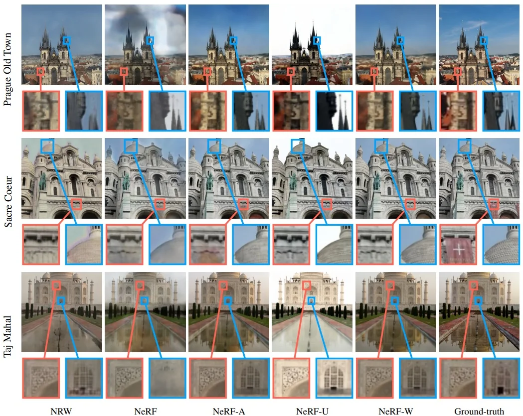
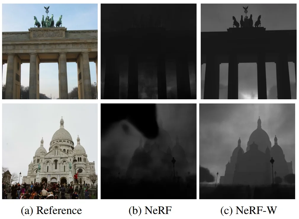
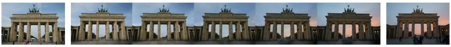
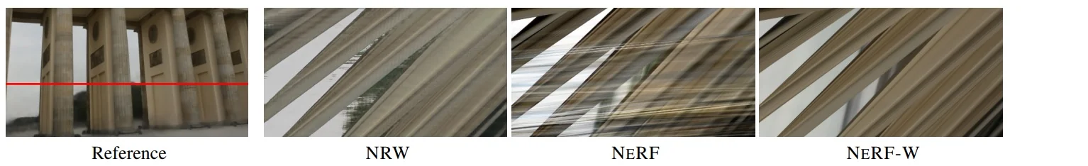
Brandenburg Gate | Sacre Coeur | Trevi Fountain | Taj Mahal | Prague | Hagia Sophia |
|||||||||||||
|---|---|---|---|---|---|---|---|---|---|---|---|---|---|---|---|---|---|---|
| PSNR | MS-SSIM | LPIPS | PSNR | MS-SSIM | LPIPS | PSNR | MS-SSIM | LPIPS | PSNR | MS-SSIM | LPIPS | PSNR | MS-SSIM | LPIPS | PSNR | MS-SSIM | LPIPS | |
| NRW [22] | 23.85 | 0.914 | 0.141 | 19.39 | 0.797 | 0.229 | 20.56 | 0.811 | 0.242 | 21.24 | 0.844 | 0.201 | 19.89 | 0.803 | 0.216 | 20.75 | 0.796 | 0.231 |
| NeRF [24] | 21.05 | 0.895 | 0.208 | 17.12 | 0.781 | 0.278 | 17.46 | 0.778 | 0.334 | 15.77 | 0.697 | 0.427 | 15.67 | 0.747 | 0.362 | 16.04 | 0.749 | 0.338 |
| NeRF-A | 27.96 | 0.941 | 0.145 | 24.43 | 0.923 | 0.174 | 26.24 | 0.924 | 0.211 | 25.99 | 0.893 | 0.225 | 22.52 | 0.870 | 0.244 | 21.83 | 0.820 | 0.276 |
| NeRF-U | 19.49 | 0.921 | 0.174 | 15.99 | 0.826 | 0.223 | 15.03 | 0.795 | 0.277 | 10.23 | 0.778 | 0.373 | 15.03 | 0.787 | 0.315 | 13.74 | 0.706 | 0.376 |
| NeRF-W | 29.08 | 0.962 | 0.110 | 25.34 | 0.939 | 0.151 | 26.58 | 0.934 | 0.189 | 26.36 | 0.904 | 0.207 | 22.81 | 0.879 | 0.227 | 22.23 | 0.849 | 0.250 |
Limitations and Future Work
Failure modes. Despite its robustness to in-the-wild photos, NeRF-W still fails in predictable ways:
Future directions.
Enrichment 23.11.3: IBRNet: Learning Multi-View Image-Based Rendering
Motivation
Problem. Given a sparse set of posed source images, synthesize photorealistic novel views of unseen scenes without any per-scene fine-tuning. A single model should generalize zero-shot to new scenes. (An optional short per-scene fine-tune can further improve fidelity; see IBRNet\(_\mbox{ft}\)).
Background: What is Image-Based Rendering (IBR)? IBR produces new views by reusing captured rays from nearby images rather than fitting a global scene-specific field. A representative classical pipeline (e.g., LLFF [441], which predates and is not based on NeRF) typically contains:
IBR preserves high-frequency appearance because it copies real image content, but its success hinges on good proxies and robust visibility reasoning under sparse views.
How NeRF differs (and how IBR can build on it). NeRF [442] represents a single scene as a continuous radiance+density field parameterized by an MLP, trained per scene by minimizing a photometric loss under differentiable volume rendering. This yields accurate geometry/appearance but requires scene-specific optimization. Modern IBR-style methods can reuse NeRF’s rendering formulation (sampling, transmittance, composition) while replacing the scene-specific field with mechanisms that aggregate multi-view image evidence on the fly. Thus, IBR can be viewed as image-conditioned rendering, whereas NeRF is scene-parameterized rendering.
Key idea. IBRNet [677] is trained once, across many diverse scenes, to interpret a small, pose–proximal set of source images from the current scene and convert them into per-ray volumetric properties that a standard NeRF-style volume renderer [442] can compose. The learned modules—a shared per-image CNN, lightweight MLP heads for visibility-aware blending and pooling, and a single-layer ray transformer that reasons along a ray—do not memorize a particular scene; instead, they encode transferable priors for fusing multi-view evidence. At test time, these same modules run in a purely feed-forward manner on the new scene’s images, so no per-scene optimization is required (a short optional fine-tune, IBRNet\(_\mbox{ft}\), can further refine thin structures and specular detail when capture is very sparse) [677].
Method: image-conditioned RGB–\(\sigma \) prediction and NeRF-style rendering
Setup and notation. Given a target camera ray \(\mathbf {r}(t)=\mathbf {o}+t\mathbf {d}\) and a small working set of \(N\) nearby source images with known intrinsics/extrinsics, IBRNet predicts, for each sampled 5D query \((\mathbf {x},\mathbf {d})\) on \(\mathbf {r}\), a color \(\mathbf {c}\in [0,1]^3\) and a density \(\sigma \ge 0\) by aggregating multi-view evidence from the source views and composing them with the standard differentiable volume renderer [442, 677]. Throughout, \(\mathbf {C}_i\) and \(\mathbf {f}_i\) denote the RGB and CNN feature sampled from source view \(i\) at the projection of \(\mathbf {x}\); \(\mathbf {d}_i\) is the source viewing direction; and \(\Delta \mathbf {d}_i=\mathbf {d}-\mathbf {d}_i\) encodes the relative direction.
Why fast and zero-shot. Per-source-view features are computed once and reused; per-sample heads are tiny MLPs; the only attention is a single, lightweight transformer along each ray. Because the scene content resides in the images and the network merely aggregates them using learned, transferable priors, a new scene needs no optimization loop—yet the same pipeline admits a brief fine-tune (IBRNet\(_\mbox{ft}\)) when desired to adapt to extreme sparsity or challenging reflectance, without altering the rendering formulation [677].
Architecture & Implementation Details
High-level architecture. IBRNet comprises three lightweight components trained jointly across many scenes [677]:
Feature extraction network.
| Input (id: dimension) | Layer | Output (id: dimension) |
|---|---|---|
| 0: \(640 \times 480 \times 3\) | \(7 \times 7\) Conv, 64, stride 2 | 1: \(320 \times 240 \times 64\) |
| 1: \(320 \times 240 \times 64\) | Residual Block 1 | 2: \(160 \times 120 \times 64\) |
| 2: \(160 \times 120 \times 64\) | Residual Block 2 | 3: \(80 \times 60 \times 128\) |
| 3: \(80 \times 60 \times 128\) | Residual Block 3 | 4: \(40 \times 30 \times 256\) |
| 5: \(40 \times 30 \times 256\) | \(3 \times 3\) Upconv, 128, factor 2 | 6: \(80 \times 60 \times 128\) |
| [3, 6]: \(80 \times 60 \times 256\) | \(3 \times 3\) Conv, 128 | 7: \(80 \times 60 \times 128\) |
| 7: \(80 \times 60 \times 128\) | \(3 \times 3\) Upconv, 64, factor 2 | 8: \(160 \times 120 \times 64\) |
| [2, 8]: \(160 \times 120 \times 128\) | \(3 \times 3\) Conv, 64 | 9: \(160 \times 120 \times 64\) |
| 9: \(160 \times 120 \times 64\) | \(1 \times 1\) Conv, 64 | Out: \(160 \times 120 \times 64\) |
| Method | #Params | #Src.Views | #FLOPs | PSNR\(\uparrow \) | SSIM\(\uparrow \) | LPIPS\(\downarrow \) |
| SRN | 0.55M | – | 5M | 22.84 | 0.668 | 0.378 |
| NeRF [442] | 1.19M | – | 304M | 26.50 | 0.811 | 0.250 |
| IBRNet\(_{\mathrm {ft}}\) | 0.04M | 5 | 29M | 25.80 | 0.828 | 0.190 |
| IBRNet\(_{\mathrm {ft}}\) | 0.04M | 8 | 45M | 26.56 | 0.847 | 0.176 |
| IBRNet\(_{\mathrm {ft}}\) | 0.04M | 10 | 55M | 26.73 | 0.851 | 0.175 |
Experiments & Ablations
Datasets and evaluation protocol. IBRNet is evaluated on three standard benchmarks: Diffuse Synthetic 360\(^\circ \) (DeepVoxels subset), Realistic Synthetic 360\(^\circ \) (NeRF synthetic), and Real Forward-Facing (LLFF forward-facing scenes). Following the original evaluation, each test view is rendered using \(N{=}10\) selected source views. Image quality is reported with PSNR/SSIM (higher is better) and LPIPS (lower is better) [677].
Baselines. The scene-agnostic (no per-scene tuning) setting is compared to LLFF [441]. The per-scene optimization setting is compared to SRN [593], NV (Neural Volumes) [401], and NeRF [442]. An optional short per-scene fine-tuning variant (IBRNet\(_\mbox{ft}\)) is also reported.
Quantitative comparison (synthetic datasets).
| Method | Setting | Diffuse Synthetic 360\(^\circ \) | Realistic Synthetic 360\(^\circ \) |
||||
|---|---|---|---|---|---|---|---|
| PSNR\(\uparrow \) | SSIM\(\uparrow \) | LPIPS\(\downarrow \) | PSNR\(\uparrow \) | SSIM\(\uparrow \) | LPIPS\(\downarrow \) | ||
| LLFF [44] | No per-scene opt. | 34.38 | 0.985 | 0.048 | 24.88 | 0.911 | 0.114 |
| IBRNet [79] | No per-scene opt. | 37.17 | 0.990 | 0.017 | 25.49 | 0.916 | 0.100 |
| SRN [42] | Per-scene opt. | 33.20 | 0.963 | 0.073 | 22.26 | 0.846 | 0.170 |
| NV [43] | Per-scene opt. | 29.62 | 0.929 | 0.099 | 26.05 | 0.893 | 0.160 |
| NeRF [37] | Per-scene opt. | 40.15 | 0.991 | 0.023 | 31.01 | 0.947 | 0.081 |
| IBRNet\(_\mbox{ft}\) [79] | Per-scene opt. | 42.93 | 0.997 | 0.009 | 28.14 | 0.942 | 0.072 |
Quantitative comparison (Real Forward-Facing).
| Method | Setting | PSNR\(\uparrow \) | SSIM\(\uparrow \) | LPIPS\(\downarrow \) |
|---|---|---|---|---|
| LLFF [44] | No per-scene opt. | 24.13 | 0.798 | 0.212 |
| IBRNet [79] | No per-scene opt. | 25.13 | 0.817 | 0.205 |
| SRN [42] | Per-scene opt. | 22.84 | 0.668 | 0.378 |
| NeRF [37] | Per-scene opt. | 26.50 | 0.811 | 0.250 |
| IBRNet\(_\mbox{ft}\) [79] | Per-scene opt. | 26.73 | 0.851 | 0.175 |
| PSNR\(\uparrow \) | SSIM\(\uparrow \) | LPIPS\(\downarrow \) | |
| No ray transformer | 21.31 | 0.675 | 0.355 |
| No view directions | 24.20 | 0.796 | 0.243 |
| Direct color regression | 24.73 | 0.810 | 0.220 |
| Full model (IBRNet) | 25.13 | 0.817 | 0.205 |
Sensitivity to source-view density. Input view sparsity denotes limiting both the number and angular spread of available source images for rendering. In the IBRNet evaluation protocol [677]:
What the figure shows and why it matters.
Per-scene fine-tuning (IBRNet\(_\mbox{ft}\)): how it is done and why it helps.
Geometry and additional results.
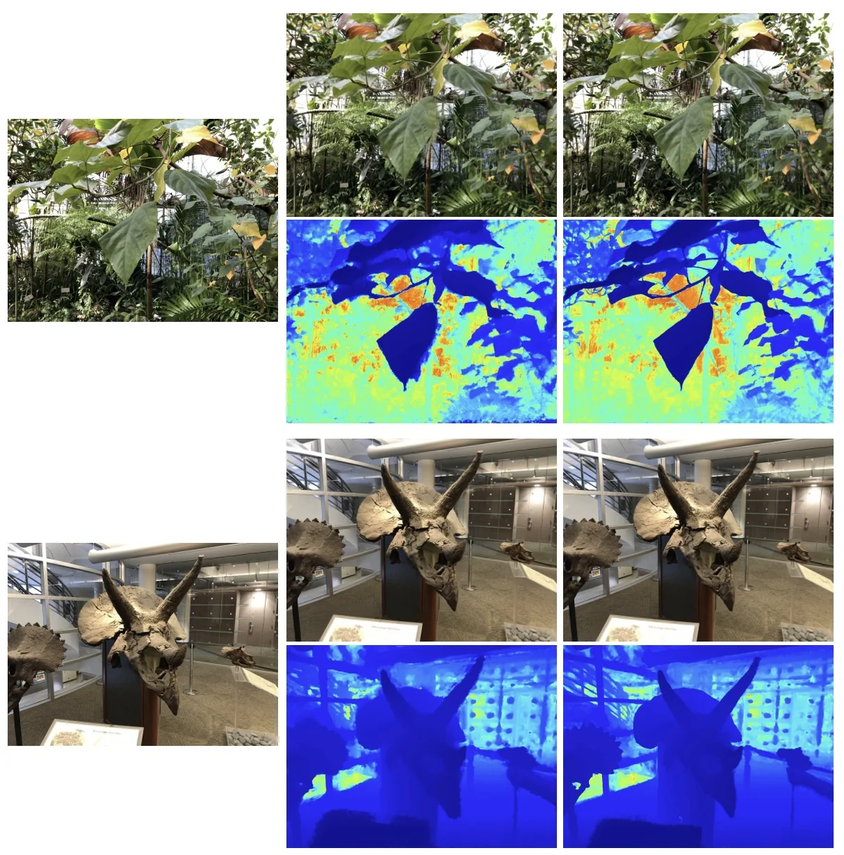
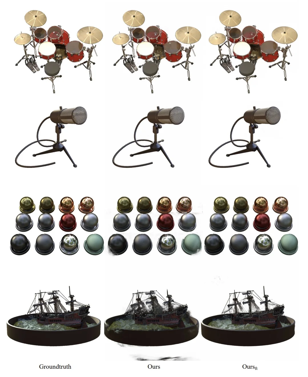
Limitations and Future Directions
Limitations. IBRNet can degrade under extremely sparse inputs and complex occlusions; although the ray transformer mitigates “black holes”, challenging specular/transparent regions may still benefit from scene-specific adaptation. Quality depends on source-view selection, pose accuracy, and coverage; thin structures and reflections improve with brief per-scene fine-tuning (IBRNet\(_\mbox{ft}\)) [677].
Concurrent and prior generalizable radiance-field methods. Several highly cited works contemporaneous with (or preceding) IBRNet pursue generalizable novel view synthesis with related but distinct designs:
Subsequent follow-ups building on IBRNet’s goals. A line of work pursues the same objective—high-quality novel views from sparse inputs with little or no per-scene optimization—by relocating where priors and visibility reasoning live in the pipeline:
Key design axes highlighted by these follow-ups.
Enrichment 23.11.4: pixelNeRF: Neural Radiance Fields from One or Few Images
Motivation
Neural Radiance Fields (NeRF) [442] achieve impressive photorealism in novel view synthesis but require dense multi-view supervision and time-intensive per-scene optimization. This limitation makes them unsuitable for scenarios with only one or few input views. PixelNeRF [762] addresses this shortcoming by learning a scene prior across multiple objects and categories, enabling feed-forward prediction of radiance fields conditioned on sparse input images. The key insight is to incorporate pixel-aligned image features into NeRF’s volumetric formulation, thereby leveraging visual evidence for generalization across scenes.
Method
PixelNeRF modifies the classical NeRF formulation by conditioning the radiance field on features extracted from input images. This conditioning transforms NeRF from a per-scene optimization problem into a feed-forward prediction pipeline that can generalize to unseen objects and scenes.
Radiance field prediction As in NeRF, the radiance field is a continuous function \[ f(\mathbf {x}, \mathbf {d}) = (\sigma , \mathbf {c}), \] that maps a 3D point \(\mathbf {x}\in \mathbb {R}^3\) and viewing direction \(\mathbf {d}\in \mathbb {R}^3\) to a density \(\sigma \) and color \(\mathbf {c}\). In NeRF, this mapping is optimized independently for each scene. PixelNeRF instead conditions \(f\) on features aligned with the input pixels.
Feature encoding and alignment An encoder \(E\) (a ResNet-34 backbone pretrained on ImageNet) processes each input image \(I\) into a pixel-aligned feature grid \(W=E(I)\). Given a query point \(\mathbf {x}\) in the camera space of an input image, PixelNeRF projects \(\mathbf {x}\) onto the image plane: \[ \pi (\mathbf {x}) = K[R \;|\; t]\mathbf {x}, \] where \(K\) are the camera intrinsics and \([R|t]\) are extrinsics. The local image feature is then sampled via bilinear interpolation: \[ \mathbf {w} = W(\pi (\mathbf {x})). \] This feature encodes appearance cues and geometric context at the projection of \(\mathbf {x}\).
Feature-conditioned NeRF The NeRF network \(f\) receives the positional encoding \(\gamma (\mathbf {x})\), the viewing direction \(\mathbf {d}\), and the interpolated feature \(\mathbf {w}\): \[ f(\gamma (\mathbf {x}), \mathbf {d}; \mathbf {w}) = (\sigma , \mathbf {c}). \] Instead of concatenating \(\mathbf {w}\) to the input, PixelNeRF injects it as a residual modulation at each layer of the MLP, inspired by style transfer methods such as AdaIN and SPADE. This design improves stability and ensures features influence the radiance field consistently across depths.
Volume rendering loss Rendered colors are computed as in NeRF: \[ \hat {C}(r) = \int _{t_n}^{t_f} T(t)\,\sigma (t)\,\mathbf {c}(t)\, dt, \quad T(t) = \exp \!\Big (-\int _{t_n}^t \sigma (s)\,ds\Big ). \] Training minimizes pixel-wise squared error: \[ \mathcal {L} = \sum _{r\in \mathcal {R}(P)} \| \hat {C}(r) - C(r)\|_2^2. \]
Why view-space conditioning Most reconstruction frameworks define radiance fields in a canonical object-centered frame, requiring all instances to share alignment. PixelNeRF instead operates in view space, i.e., the coordinate frame of each input camera. This removes the need for a canonical alignment, improving generalization to unseen categories, multiple-object scenes, and real-world captures where canonical orientation does not exist.
Multi-view extension For multiple input images \(\{I^{(i)}\}_{i=1}^n\) with poses \(P^{(i)}=[R^{(i)}|t^{(i)}]\), query points are transformed into each view: \[ \mathbf {x}^{(i)} = P^{(i)}\mathbf {x}, \qquad \mathbf {d}^{(i)} = R^{(i)}\mathbf {d}. \] Each view provides intermediate features: \[ V^{(i)} = f_1(\gamma (\mathbf {x}^{(i)}), \mathbf {d}^{(i)}; W^{(i)}(\pi (\mathbf {x}^{(i)}))). \] These are pooled using an order-independent operator \(\psi \) (average pooling) and passed to a final network \(f_2\): \[ (\sigma , \mathbf {c}) = f_2(\psi (V^{(1)}, \dots , V^{(n)})). \] This architecture allows variable numbers of input images at test time without retraining.
Intuition and significance PixelNeRF can be understood as embedding a strong inductive bias into NeRF: each query point consults features sampled from projected 2D observations. This design provides two critical benefits: (1) appearance grounding, since colors derive from aligned image evidence; and (2) geometric priors, since features across views encode spatial structure. Consequently, PixelNeRF learns to hallucinate plausible completions when input views are sparse, a task impossible for vanilla NeRF.
Architecture and Implementation
PixelNeRF uses a ResNet-34 encoder with a feature pyramid to capture local and global cues. Features from multiple scales are upsampled and concatenated, resulting in \(512\)-dimensional descriptors aligned with image pixels. The NeRF network \(f\) is implemented as a residual MLP. Instead of concatenating features directly, linear layers map each feature vector into per-block residuals added within ResNet blocks. This design stabilizes training and enables feature modulation across layers.
Experiments and Ablations
PixelNeRF is evaluated across category-specific (chairs, cars), category-agnostic (13 ShapeNet classes), unseen categories, multi-object scenes, and real-world datasets (Stanford Cars; DTU MVS), demonstrating consistent gains over SRN [593] and DVR [465]. Ablations confirm the necessity of pixel-aligned local features and view-direction inputs.
Category-specific single-view reconstruction A separate PixelNeRF is trained per category using multi-view 2D supervision; qualitative examples include a chair, sofa, van, and police car.
Category-specific two-view reconstruction Two input images are encoded; two novel renderings are shown per example for chairs and cars.
| Method | 1-view | 2-view | ||
|---|---|---|---|---|
| PSNR\(\uparrow \) | SSIM\(\uparrow \) | PSNR\(\uparrow \) | SSIM\(\uparrow \) | |
Chairs | ||||
| GRF [103] | 21.25 | 0.86 | 22.65 | 0.88 |
| TCO\(^\ast \) [107] | 21.27 | 0.88 | 21.33 | 0.88 |
| dGQN [108] | 21.59 | 0.87 | 22.36 | 0.89 |
| ENR\(^\ast \) [109] | 22.83 | – | – | – |
| SRN [42] | 22.89 | 0.89 | 24.48 | 0.92 |
| PixelNeRF\(^\ast \) [78] | 23.72 | 0.91 | 26.20 | 0.94 |
Cars |
||||
| SRN [42] | 22.25 | 0.89 | 24.84 | 0.92 |
| ENR\(^\ast \) [109] | 22.26 | – | – | – |
| PixelNeRF\(^\ast \) [78] | 23.17 | 0.90 | 25.66 | 0.94 |
Ablation on local features and view directions Goal This ablation on ShapeNet chairs isolates the contributions of two architectural choices in PixelNeRF [762]: pixel-aligned local features and explicit view directions. The objective is to determine how each component affects few-shot reconstruction quality in single-view and two-view settings within PixelNeRF’s viewer-centric, feed-forward formulation.
Design of the variants
Mechanism and expected effects PixelNeRF uses a ResNet-34 encoder to produce a multi-scale feature pyramid that is upsampled and concatenated into \(\sim \)512-D descriptors aligned to input pixels. For a 3D query point \(\mathbf {x}\), the point is projected to each input image, and a bilinearly interpolated feature \(\mathbf {w}=W(\pi (\mathbf {x}))\) modulates the NeRF MLP through residual injections at block entrances. This pixel-level conditioning supplies localized appearance and geometry cues tied to \(\mathbf {x}\)’s projections. Removing local features (-- Local) collapses this spatially precise conditioning to a global code, reducing fidelity in thin structures and high-frequency textures. Removing directions (-- Dirs) suppresses view-dependent modeling, impairing consistency under large baselines or glossy surfaces.
Findings The following table shows that both components are important. Relative to Full, -- Local exhibits noticeable drops in PSNR/SSIM and worse LPIPS, indicating that pixel-aligned evidence is helpful for accurate shape and texture reconstruction from few views. -- Dirs also degrades all metrics, confirming the choice of using explicit viewing direction inputs for high-fidelity, view-dependent rendering. The Full model achieves the best performance in both 1-view and 2-view settings.
| Variant | 1-view | 2-view | ||||
|---|---|---|---|---|---|---|
| PSNR\(\uparrow \) | SSIM\(\uparrow \) | LPIPS\(\downarrow \) | PSNR\(\uparrow \) | SSIM\(\uparrow \) | LPIPS\(\downarrow \) | |
| – Local | 20.39 | 0.848 | 0.196 | 21.17 | 0.865 | 0.175 |
| – Dirs | 21.93 | 0.885 | 0.139 | 23.50 | 0.909 | 0.121 |
| Full | 23.43 | 0.911 | 0.104 | 25.95 | 0.939 | 0.071 |
Category-agnostic single-view reconstruction A single PixelNeRF trained jointly on the 13 largest ShapeNet categories preserves thin structures and small textures, while outperforming baselines quantitatively (exactly as reported).
| plane | bench | cbnt. | car | chair | disp. | lamp | spkr. | rifle | sofa | table | phone | boat | mean | |
| \(\uparrow \) PSNR | ||||||||||||||
| DVR [106] | 25.29 | 22.64 | 24.47 | 23.95 | 19.91 | 20.86 | 23.27 | 20.78 | 23.44 | 23.35 | 21.53 | 24.18 | 25.09 | 22.70 |
| SRN [42] | 26.62 | 22.20 | 23.42 | 24.40 | 21.85 | 19.07 | 22.17 | 21.04 | 24.95 | 23.65 | 22.45 | 20.87 | 25.86 | 23.28 |
| PixelNeRF [78] | 29.76 | 26.35 | 27.72 | 27.58 | 23.84 | 24.22 | 28.58 | 24.44 | 30.60 | 26.94 | 25.59 | 27.13 | 29.18 | 26.80 |
| \(\uparrow \) SSIM | ||||||||||||||
| DVR [106] | 0.905 | 0.866 | 0.877 | 0.909 | 0.787 | 0.814 | 0.849 | 0.798 | 0.916 | 0.868 | 0.840 | 0.892 | 0.902 | 0.860 |
| SRN [42] | 0.901 | 0.837 | 0.831 | 0.897 | 0.814 | 0.744 | 0.801 | 0.779 | 0.913 | 0.851 | 0.828 | 0.811 | 0.898 | 0.849 |
| PixelNeRF [78] | 0.947 | 0.911 | 0.910 | 0.942 | 0.858 | 0.867 | 0.913 | 0.855 | 0.968 | 0.908 | 0.898 | 0.922 | 0.939 | 0.910 |
| \(\downarrow \) LPIPS | ||||||||||||||
| DVR [106] | 0.095 | 0.129 | 0.125 | 0.098 | 0.173 | 0.150 | 0.172 | 0.170 | 0.094 | 0.119 | 0.139 | 0.110 | 0.116 | 0.130 |
| SRN [42] | 0.111 | 0.150 | 0.147 | 0.115 | 0.152 | 0.197 | 0.210 | 0.178 | 0.111 | 0.129 | 0.135 | 0.165 | 0.134 | 0.139 |
| PixelNeRF [78] | 0.084 | 0.116 | 0.105 | 0.095 | 0.146 | 0.129 | 0.114 | 0.141 | 0.066 | 0.116 | 0.098 | 0.097 | 0.111 | 0.108 |
Unseen categories and multi-object scenes Training only on plane, car, chair, PixelNeRF generalizes to 10 unseen categories and handles composed scenes of multiple chairs by predicting in view space.
Real images: Stanford Cars and DTU MVS A car model transfers to Stanford Cars after background removal with PointRend; on DTU, feed-forward wide-baseline synthesis is demonstrated from three posed inputs; PSNR quantiles versus per-scene NeRF are reported in the paper.
Limitations and Future Work
Future work and influence PixelNeRF inspired numerous follow-ups addressing its limitations:
These directions show how PixelNeRF provided the first bridge between feed-forward image-conditioned priors and NeRF-based volumetric rendering, catalyzing a wave of methods tackling sparse-view reconstruction and real-world generalization.
Enrichment 23.12: NeRF: Unbounded, Dynamic, Large-Scale Scenes
Scaling beyond tabletop scenes requires anti-aliasing across scales, compositional scene structure, and deformation fields for motion.
Further influential works (not expanded): HyperNeRF [482] (handles topological changes in dynamic scenes), Mega-NeRF [426] (city-to-landscape scale).
Enrichment 23.12.1: Block-NeRF: Scalable Large Scene Neural View Synthesis
Motivation
Neural Radiance Fields (NeRF) and its multiscale extension mip-NeRF (see Enrichment 23.10.5) have demonstrated remarkable performance on small-scale, object-centric, or single-building scenes. However, scaling such methods to city-sized environments introduces severe bottlenecks: limited model capacity, memory constraints, and inconsistent appearance due to data collected across different days, times, and weather conditions. For practical applications in mapping and autonomous driving, the ability to reconstruct neighborhoods with temporal consistency and update regions without retraining the full model is crucial. Block-NeRF [623] introduces a decomposition strategy that splits the environment into compact, geographically bounded NeRFs (blocks). Each block is trained independently and later merged at inference to produce seamless renderings, decoupling rendering cost from the overall environment size.
Method
High-level overview Block-NeRF [623] scales neural view synthesis to neighborhoods by structuring the scene geographically and decoupling capacity and rendering from global extent. The pipeline proceeds in four stages:
Block partitioning and structure The partitioning strategy employed by Block-NeRF is designed to make large-scale reconstruction, such as multi-block urban scenes, tractable by dividing the environment into smaller, manageable sub-regions. Instead of training one monolithic NeRF for an entire city—which would exceed memory and compute limits—Block-NeRF constructs a structured grid of compact NeRFs that can be trained and updated independently.
Why overlapping sub-regions? Each Block-NeRF is defined to overlap about 50% with its neighbors. This deliberate redundancy serves two roles:
During inference, this overlap also supports seamless compositing when multiple blocks contribute to a target view, avoiding visual jumps at block boundaries.
Why place origins at intersections? Block origins are typically anchored at road intersections. Intersections serve as natural hubs in city topology: they connect multiple streets, maximize shared visibility across trajectories, and ensure that blocks cover semantically meaningful spatial units. Placing block centers at intersections also yields a regular, interpretable tiling of the urban grid. In practice, a block covers its local intersection and extends along adjacent streets.
How are partitions built? From these origins, each block’s coverage extends roughly 75% of the way to neighboring intersections. This produces the desired \(\sim 50\%\) overlap across adjacent blocks. Building the partitions proceeds as follows:
This decomposition yields a scalable representation: a city becomes a grid of compact NeRFs with intentional redundancy at boundaries. The overlap is key not only for geometric continuity but also for appearance alignment, enabling Block-NeRF to harmonize heterogeneous data collected across days, weather conditions, and camera settings.
Architectural design choices Each Block-NeRF extends mip-NeRF with three critical augmentations:
In addition, a lightweight visibility network \(f_v\) is trained to predict whether a spatial sample would be visible from a given camera viewpoint. Unlike computing transmittance \(T\) directly from each block’s density field (which requires full ray marching), \(f_v\) is a cheap learned proxy supervised by training-time transmittance. This decoupled approximation plays two roles in the Block-NeRF pipeline: (i) block selection at inference, where it prevents unnecessary evaluation of irrelevant or occluded blocks, and (ii) appearance matching, where it identifies reliable overlap regions between neighboring blocks for cross-block alignment.
How \(f_v\) integrates into the pipeline During training. For every training ray, Block-NeRF already computes sample weights \[ T_i = \exp \!\Big (-\sum _{j<i} \sigma _j \delta _j\Big ), \] the transmittance at depth \(t_i\). These values supervise \(f_v(\mathbf {x}_i,\mathbf {d})\) at sampled points, teaching the auxiliary network to approximate visibility directly from \((\mathbf {x},\mathbf {d})\) without performing volume accumulation. Thus \(f_v\) becomes a fast surrogate of NeRF’s own visibility reasoning.
During inference. Given a novel camera:
Why \(f_v\) is essential Without \(f_v\), Block-NeRF would need to partially render all nearby blocks to check visibility. This is computationally intractable for hundreds of blocks. \(f_v\) serves as a fast scout: trained once during supervision, then deployed at inference to prune irrelevant blocks and guide alignment. This makes city-scale rendering practical while preserving seamless transitions across block boundaries.
Compositing across blocks After visibility pruning, the surviving blocks are rendered with mip-NeRF’s volumetric ray marching (Sec. Enrichment 23.10.5). Their outputs \(\mathbf {I}_i\) are then blended in raster space using inverse-distance weights relative to the camera: \[ w_i \propto \|c - x_i\|^{-p}, \qquad \sum _i w_i = 1, \] with \(p\) controlling the sharpness of transitions. This global weighting strategy is simple to compute, avoids per-pixel overhead, and—most importantly—yields temporally stable results for long flythroughs. In practice, distance-based blending reliably hides seams in overlap regions; more complex schemes (e.g., depth- or visibility-based blending) can sharpen stills but often introduce flicker over time.
Appearance control and cross-block alignment A remaining challenge is that independently trained blocks do not share a common appearance embedding space: the same latent index can correspond to different global looks (e.g., sunny in one block, cloudy in another). When blended directly, such inconsistencies manifest as visible seams. To harmonize the output, Block-NeRF performs appearance matching across overlaps:
This process aligns low-frequency appearance factors such as illumination, weather, and time-of-day, producing a globally coherent style while preserving local geometry. Once aligned, the entire city-scale environment can be rendered consistently under any desired appearance (e.g., dusk everywhere).
Why this design works Geographic tiling concentrates capacity where needed and enables local updates. Visibility-driven selection avoids wasting compute and prevents seam artifacts from blocks that cannot explain the view. Distance-based blending is temporally stable and simple. Appearance embeddings + exposure conditioning disentangle nuisance factors (time, weather, camera settings) from scene structure, while appearance matching reconciles independently trained blocks into a coherent city-scale radiance field.
Experiments and Ablations
Ablations on Alamo Square Appearance embeddings, exposure conditioning, and pose refinement all contribute significantly to fidelity. Removing appearance embeddings forces the model to encode weather variations as geometry, introducing artifacts. Disabling pose refinement produces blur and duplication from misalignment. Removing exposure slightly lowers accuracy but eliminates exposure control.
| Model | PSNR\(\uparrow \) | SSIM\(\uparrow \) | LPIPS\(\downarrow \) |
| mip-NeRF [57] | 17.86 | 0.563 | 0.509 |
| -Block-NeRF (no appearance) | 20.13 | 0.611 | 0.458 |
| -Block-NeRF (no exposure) | 23.55 | 0.649 | 0.418 |
| -Block-NeRF (no pose opt.) | 23.05 | 0.625 | 0.442 |
| Full Block-NeRF | 23.60 | 0.649 | 0.417 |
Block granularity on Mission Bay Splitting into finer blocks improves accuracy even when the total parameter count is fixed. With smaller block sizes, each block specializes to local geometry and appearance, and only a few blocks are active per frame, keeping inference efficient.
| # Blocks | Weights / Total | Block size | Compute | PSNR\(\uparrow \) | SSIM\(\uparrow \) | LPIPS\(\downarrow \) |
| 1 | 0.25M / 0.25M | 544 m | \(1\times \) | 23.83 | 0.825 | 0.381 |
| 4 | 0.25M / 1.00M | 271 m | \(2\times \) | 25.55 | 0.868 | 0.318 |
| 8 | 0.25M / 2.00M | 116 m | \(2\times \) | 26.59 | 0.890 | 0.278 |
| 16 | 0.25M / 4.00M | 54 m | \(2\times \) | 27.40 | 0.907 | 0.242 |
| 1 | 1.00M / 1.00M | 544 m | \(1\times \) | 24.90 | 0.852 | 0.340 |
| 4 | 0.25M / 1.00M | 271 m | \(0.5\times \) | 25.55 | 0.868 | 0.318 |
| 8 | 0.13M / 1.00M | 116 m | \(0.25\times \) | 25.92 | 0.875 | 0.306 |
| 16 | 0.07M / 1.00M | 54 m | \(0.125\times \) | 25.98 | 0.877 | 0.305 |
Limitations and Future Work
Block-NeRF inherits Mip-NeRF’s high rendering cost and struggles with unmasked dynamic content. Transient objects leave artifacts such as shadows; vegetation and seasonal changes lead to blurred trees; construction requires retraining of affected blocks. Distant structures are under-sampled, producing lower fidelity. Future directions to combat these and improve results include:
Enrichment 23.12.2: Mip-NeRF 360: Unbounded Anti-Aliased NeRF
Motivation
Real-world unbounded scenes (full 360° rotations, sky and horizons, distant buildings) reveal persistent weaknesses in NeRF-style pipelines: distant regions render blurry, scaling capacity becomes costly, and ambiguity induces artifacts such as semi-transparent floaters and background collapse. Readers are referred to the prior subsection on mip-NeRF for anti-aliasing via integrated positional encoding (IPE) over conical-frustum Gaussians (§Enrichment 23.10.5) [29]. MipNeRF360 [28] builds on that foundation to make 360° unbounded scenes numerically well-posed, sample-efficient, and less ambiguous.
Challenges in unbounded 360° scenes
MipNeRF360 solutions to unbounded scenes challenges
Method
MipNeRF360 extends mip-NeRF (§Enrichment 23.10.5) to unbounded 360° scenes with three coupled components: a smooth nonlinear scene reparameterization that makes “infinity” finite while preserving near-camera geometry; a proposal-driven hierarchical sampling scheme that decouples where to sample from what to predict via online histogram consistency; and a distortion regularizer that shapes per-ray weight distributions to suppress floaters and discourage background collapse [28].
Preliminaries: mip-NeRF For a ray \(\mathbf {r}(t)=\mathbf {o}+t\mathbf {d}\) with distances \(t=\{t_i\}_{i=0}^{N}\) partitioning intervals \(T_i=[t_i,t_{i+1})\), mip-NeRF approximates each conical frustum by a 3D Gaussian with mean \(\boldsymbol \mu \) and covariance \(\boldsymbol \Sigma \) and featurizes it with integrated positional encoding (IPE): \begin {equation} \gamma (\boldsymbol \mu ,\boldsymbol \Sigma )=\left \{\! \begin {bmatrix} \sin (2^{\ell }\boldsymbol \mu )\,\exp \!\big (-2^{2\ell -1}\operatorname {diag}(\boldsymbol \Sigma )\big )\\ \cos (2^{\ell }\boldsymbol \mu )\,\exp \!\big (-2^{2\ell -1}\operatorname {diag}(\boldsymbol \Sigma )\big ) \end {bmatrix} \right \}_{\ell =0}^{L-1} \label {eq:mipnerf_ipe} \end {equation} These features drive an MLP (NeRF MLP) to produce density \(\tau _i\) and color \(\mathbf {c}_i\): \begin {equation} (\tau _i,\mathbf {c}_i)=\mathrm {MLP}\!\big (\gamma (\mathbf {r}(T_i));\Theta _{\mbox{NeRF}}\big ) \label {eq:mipnerf_mlp} \end {equation} Pixel color is rendered by volumetric compositing: \begin {align} \mathbf {C}(\mathbf {r},t) &= \sum _i w_i\,\mathbf {c}_i, \label {eq:mipnerf_color}\\ w_i &= \big (1-e^{-\tau _i\,(t_{i+1}-t_i)}\big )\exp \!\Big (-\sum _{i'<i}\tau _{i'}(t_{i'+1}-t_{i'})\Big ) \label {eq:mipnerf_weights} \end {align}
Coarse intervals are sampled uniformly in \([t_n,t_f]\): \begin {equation} t^{\mathrm {c}}\sim \mathcal {U}[t_n,t_f],\qquad t^{\mathrm {c}}=\mathrm {sort}(\{t^{\mathrm {c}}\}) \label {eq:mipnerf_tc} \end {equation} then refined via inverse-transform sampling from the coarse histogram: \begin {equation} t^{\mathrm {f}}\sim \mathrm {hist}\!\big (t^{\mathrm {c}},w^{\mathrm {c}}\big ),\qquad t^{\mathrm {f}}=\mathrm {sort}(\{t^{\mathrm {f}}\}) \label {eq:mipnerf_tf} \end {equation} Training minimizes a weighted sum of coarse/fine reconstruction losses: \begin {equation} \sum _{\mathbf {r}\in \mathcal {R}}\frac {1}{10}\,\mathcal {L}_{\mathrm {recon}}\big (\mathbf {C}(\mathbf {r},t^{\mathrm {c}}),\mathbf {C}^\ast (\mathbf {r})\big )\;+\;\mathcal {L}_{\mathrm {recon}}\big (\mathbf {C}(\mathbf {r},t^{\mathrm {f}}),\mathbf {C}^\ast (\mathbf {r})\big ) \label {eq:mipnerf_loss} \end {equation} See §Enrichment 23.10.5 for details [29].
Scene and ray parameterization Context and goal. In mip-NeRF, each ray interval (a conical frustum) is approximated by a 3D Gaussian with mean \(\boldsymbol \mu \) and covariance \(\boldsymbol \Sigma \), and features are computed directly in Euclidean coordinates via integrated positional encoding (IPE). For truly unbounded 360° scenes, this Euclidean parameterization becomes ill-conditioned at long range. MipNeRF360 changes where those features are computed: it first reparameterizes the scene by a smooth warp \(f:\mathbb {R}^3\!\to \!\mathbb {R}^3\) that makes infinity finite, and only then encodes the frustum-Gaussians. This has two consequences. First, the Gaussian must be pushed through the nonlinear \(f\) so that both its center and its spatial extent are correctly warped. Second, ray distances must be reparameterized to align sample placement with the new geometry. Together, these steps define MipNeRF360’s scene and ray parameterization [28].
Pushing Gaussians through a smooth warp (Eq. 9). Because \(f\) is nonlinear, the image of a Gaussian is not Gaussian in closed form. MipNeRF360 therefore adopts the standard first–order (Extended Kalman Filter–style) approximation: linearize \(f\) at the mean and propagate mean and covariance through that local linear map, \begin {equation} f(\mathbf {x}) \approx f(\boldsymbol \mu ) + J_f(\boldsymbol \mu )\,(\mathbf {x}-\boldsymbol \mu ), \qquad f(\boldsymbol \mu ,\boldsymbol \Sigma ) \;=\; \Big (f(\boldsymbol \mu ),\; J_f(\boldsymbol \mu )\,\boldsymbol \Sigma \,J_f(\boldsymbol \mu )^\top \Big ). \label {eq:linearize-push} \end {equation} Here \(J_f(\boldsymbol \mu )\) is the \(3{\times }3\) Jacobian of \(f\) at \(\boldsymbol \mu \), capturing the local stretch/rotation induced by \(f\). This “Kalman-like” pushforward is essential: it preserves not only the warped position \(f(\boldsymbol \mu )\) but also the warped extent and orientation \(J_f\boldsymbol \Sigma J_f^\top \) of the frustum. Without updating the covariance, far-field frustums—often highly anisotropic—would be misrepresented after warping, undermining mip-NeRF’s anti-aliasing.
Choosing the warp: contraction (Eq. 10). In MipNeRF360 the scene warp \(f\) is a smooth contraction that maps all of \(\mathbb {R}^3\) into a closed ball of radius \(2\) while leaving the unit ball unchanged: \begin {equation} f(\mathbf {x}) \;=\; \operatorname {contract}(\mathbf {x}) \;=\; \begin {cases} \mathbf {x}, & \|\mathbf {x}\|\le 1,\\[4pt] \Bigl (2-\dfrac {1}{\|\mathbf {x}\|}\Bigr )\dfrac {\mathbf {x}}{\|\mathbf {x}\|}, & \|\mathbf {x}\|>1. \end {cases} \label {eq:contract} \end {equation} Why keep \(\|\mathbf {x}\|\!\le \!1\) unchanged, and why a shell \([1,2]\) for the far field? The unit ball fixes a normalized near-field scale around the camera where small metric errors drive perceived sharpness (parallax, fine texture). Keeping \(f(\mathbf {x})=\mathbf {x}\) there preserves exact Euclidean geometry and the anti-aliasing behavior inherited from mip-NeRF. Mapping everything beyond the unit sphere into the finite shell \(1\!\to \!2\) preserves dynamic range for large depths: depths just beyond \(1\) map near \(1\), while depths \(\|\mathbf {x}\|\!\to \!\infty \) map smoothly toward \(2\)—so “far” and “very far” remain separable after warping, instead of collapsing onto a single boundary. Because the target is spherical, all directions are treated symmetrically.
Why this reduces common failure modes (mechanism, not just outcome):
After pushing the frustum-Gaussian \((\boldsymbol \mu ,\boldsymbol \Sigma )\) through \(f\) via the linearization in Eq. (23.52), features are computed from the contracted Gaussian \[ \gamma \!\big (\operatorname {contract}(\boldsymbol \mu ,\boldsymbol \Sigma )\big ), \] so within-interval anti-aliasing is preserved but now in a bounded, well-conditioned coordinate system [28].
Off-axis IPE—where it fits and why it matters After the scene is contracted and each frustum-Gaussian \((\boldsymbol \mu ,\boldsymbol \Sigma )\) is pushed through the warp using the EKF-style update in Eq. (23.52), MipNeRF360 computes features in the contracted space with Integrated Positional Encoding (IPE). IPE is mip-NeRF’s anti-aliasing mechanism: instead of encoding a single point, it encodes the expected sine/cosine responses under the Gaussian, so pixel footprint and frustum extent are baked into the features. In the original, axis-aligned version, these sinusoids are taken along the coordinate axes, which means only the diagonal of \(\boldsymbol \Sigma \) (per-axis variance) can modulate the features.
The contraction plus the Kalman-like pushforward typically yields full, rotated covariances in the warped space—far-field frustums are elongated and oriented off-axis—so restricting IPE to axis directions discards the very orientation cues that distinguish different Gaussians. MipNeRF360 therefore adopts off-axis IPE (Appendix of [28]): it projects the Gaussian onto a fixed bank of non-axis-aligned unit directions (the vertices of a twice-tessellated icosahedron), allowing off-diagonal covariance to influence the features. Intuitively, two Gaussians can share the same per-axis spreads yet differ in orientation; axis-aligned IPE conflates them, while off-axis IPE keeps them separate. The result is a richer, orientation-sensitive encoding of elongated, distant frustums, which improves discrimination and stability in the far field [28].
Reparameterizing the ray: disparity-linear coordinate (Eq. 11). The contraction makes the space finite; the ray parameter determines how samples populate that space. MipNeRF360 maps Euclidean distance \(t\!\in [t_n,t_f]\) to a normalized coordinate \(s\!\in [0,1]\) via an invertible \(g\): \begin {equation} s \;=\; \frac {g(t)-g(t_n)}{g(t_f)-g(t_n)},\qquad t \;=\; g^{-1}\!\big (s\,g(t_f)+(1-s)\,g(t_n)\big ), \label {eq:s-mapping} \end {equation} and sets \(g(x)=1/x\) so bins are uniform in inverse depth (disparity). Why \(s\) (disparity) behaves better than \(t\) (metric depth):
Together, Eq. (10) makes “infinity” finite with preserved depth resolution, and Eq. (11) distributes a fixed number of samples where the image is most sensitive—yielding sharper backgrounds, fewer collapse incentives, and more stable optimization in unbounded 360° scenes [28].
Coarse-to-fine online distillation Where this fits in the pipeline. Having reparameterized the scene with the contraction \(f\) and the ray with the disparity-linear coordinate \(s\) (Sec. Enrichment 23.12.2), MipNeRF360 must still decide where along \(s\in [0,1]\) to place computation. Rather than supervising a single MLP at multiple scales (mip-NeRF), MipNeRF360 separates where to sample from what to predict: a lightweight network proposes sampling distributions along the ray, and a high-capacity network predicts densities and colors [28].
Two-MLP cascade. The model uses (i) a small proposal MLP that outputs only densities (hence interval weights, no colors), and (ii) a large NeRF MLP that outputs both density and color. Work proceeds along the normalized coordinate \(s\):
From proposal to final histogram. Building on the two–MLP cascade, each ray is processed in two stages: (i) one or two proposal passes produce a coarse, then refined sampling partition together with a coarse weight histogram; (ii) a single final pass evaluates the high-capacity NeRF MLP on the last, content-focused partition to obtain the weights and colors used for rendering. The proposal is trained to safely guide the final pass via a one-sided consistency loss; the NeRF MLP is trained by the usual image reconstruction (and later, distortion) losses. Crucially, the consistency loss uses stop-gradient on the NeRF outputs so that NeRF “leads” and the proposal “follows”, preventing the two networks from colluding by making NeRF artificially easier to cover [28].
Notation and partitions (one ray). Along a ray we keep a 1D histogram: a strictly increasing list of bin edges and one nonnegative weight per bin that sums to \(1\). During the proposal stage the small network is evaluated on a coarse partition, yielding a proposal histogram with edges \(\hat {t}=\{\hat {t}_j\}_{j=0}^{\hat {M}}\) and weights \(\hat {w}=\{\hat {w}_j\}_{j=1}^{\hat {M}}\) (weights computed from proposal densities via standard NeRF compositing). After importance resampling around peaks of \(\hat {w}\), we obtain a refined partition on which the NeRF MLP is run once to produce the final histogram \((t,w)\) with edges \(t=\{t_i\}_{i=0}^{M}\) and weights \(w=\{w_i\}_{i=1}^{M}\). Typically \(\hat {M}\!<\!M\) and proposal bins are wider. This is an intended difference in bin counts/widths that we denote as different “step size”. Because the refined edges are created from the coarse proposal via resampling, the two partitions need not align; they are allowed to be misaligned by design.
About coordinates. The paper actually samples and resamples in the disparity-linear coordinate \(s\!\in [0,1]\). For notational continuity we write edges as \(t\), but you can read \(t\) as “whatever monotone ray coordinate is used to lay out edges” (in practice, \(t\equiv s\) here). This choice does not affect the consistency machinery: the check asks whether a final interval \(T_i=[t_i,t_{i+1})\) is covered by the coarse proposal, which we test by summing proposal weights over all proposal bins that overlap \(T_i\). Summing over overlaps depends only on which portions of the ray are covered, not on how those portions are parametrized, so it remains valid even when the two histograms have different edge locations, widths, or numbers of bins.
Histogram-consistency bound (Eqs. 12–13). The proposal is trained with a one-sided don’t-miss-mass constraint so that importance resampling can always find regions the final pass relies on. Let the final bins be \(T_i=[t_i,t_{i+1})\) and the proposal bins be \(\hat {T}_j=[\hat {t}_j,\hat {t}_{j+1})\). Define the overlap-based bound for any interval \(T\): \begin {equation} \mathrm {bound}(\hat {t},\hat {w},T)\;=\;\sum _{j:\,T\cap \hat {T}_j\neq \emptyset }\hat {w}_j. \label {eq:bound} \end {equation} Consistency requires \(w_i \le \mathrm {bound}(\hat {t},\hat {w},T_i)\) for all \(i\). Any excess final mass above this bound is penalized: \begin {equation} \mathcal {L}_{\mathrm {prop}}(t,w,\hat {t},\hat {w}) \;=\; \sum _i \frac {1}{w_i}\,\max \!\Bigl (0,\,w_i-\mathrm {bound}(\hat {t},\hat {w},T_i)\Bigr )^2, \label {eq:lprop} \end {equation} with stop-gradient on \((t,w)\) so that only the proposal MLP is updated.
Intuition.
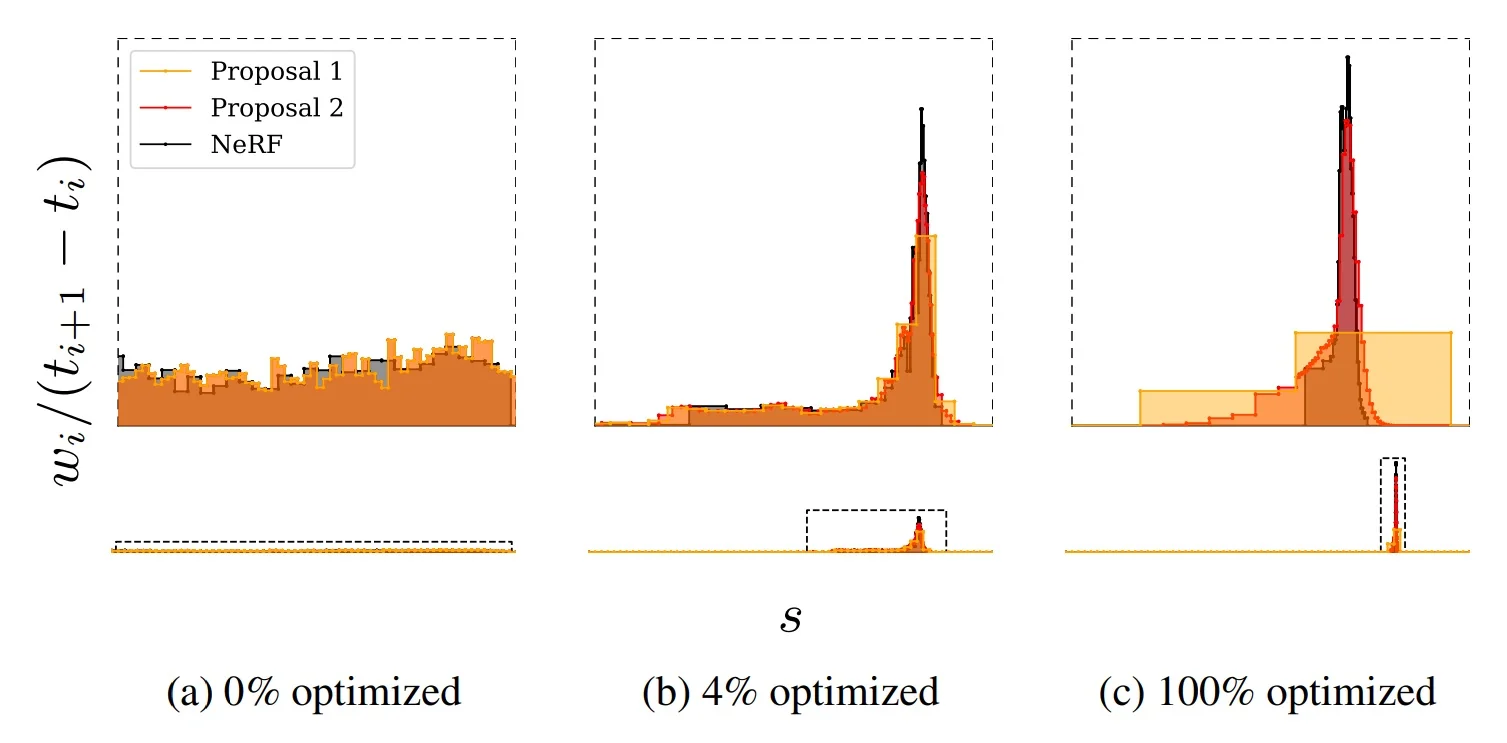
Sampling refinements: what they do and why they help.
Regularization for interval-based models Even with contraction and proposal guidance, the inverse problem remains ambiguous along the ray: colors can be matched by distributing small weights across many separated intervals (floaters) or by shifting mass toward the camera (background collapse). MipNeRF360 therefore adds a distortion loss on the per-ray step function \(w_s(\cdot )=\sum _i w_i\,\mathbf {1}_{[s_i,s_{i+1})}(\cdot )\) over \(s\!\in [0,1]\): \begin {equation} \mathcal {L}_{\mathrm {dist}}(s,w)=\int \!\!\int w_s(u)\,w_s(v)\,|u-v|\,\mathrm {d}u\,\mathrm {d}v. \label {eq:ldist_integral} \end {equation} Evaluated on piecewise-constant histograms, this yields the efficient discrete form \begin {equation} \mathcal {L}_{\mathrm {dist}}(s,w)=\sum _{i,j} w_i w_j\left |\frac {s_i+s_{i+1}}{2}-\frac {s_j+s_{j+1}}{2}\right |+\frac {1}{3}\sum _i w_i^2\,(s_{i+1}-s_i). \label {eq:ldist_discrete} \end {equation} The pairwise-midpoint term penalizes spreading weight across distant intervals, while the width term penalizes placing large mass in wide bins. Minimizing \(\mathcal {L}_{\mathrm {dist}}\) thus favors compact, minimally fragmented weight layouts consistent with the image evidence, which suppresses floaters and reduces the incentive for background collapse. Gradients of this loss naturally pull nearby weighted intervals together, shrink overly wide bins, and drive weights to zero when a ray is empty [28].
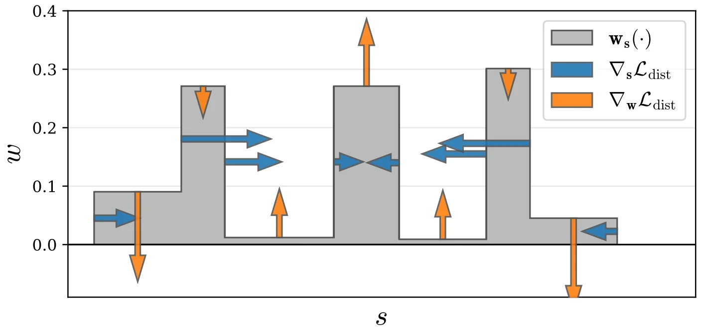
Optimization and training recipe Network sizes and sampling. The proposal MLP uses \(4\) layers with \(256\) hidden units; the NeRF MLP uses \(8\) layers with \(1024\) units; ReLU internals and softplus density. Two proposal stages are evaluated (each with \(64\) samples) to produce \((\hat {s}^{(0)},\hat {w}^{(0)})\) and \((\hat {s}^{(1)},\hat {w}^{(1)})\), followed by one NeRF stage with \(32\) samples to produce \((s,w)\) [28].
Loss. The overall objective is \begin {equation} \mathcal {L}=\mathcal {L}_{\mathrm {recon}}(\mathbf {C}(t),\mathbf {C}^\ast )+\lambda \,\mathcal {L}_{\mathrm {dist}}(s,w)+\sum _{k=0}^{1}\mathcal {L}_{\mathrm {prop}}\!\big (s,w,\hat {s}^{(k)},\hat {w}^{(k)}\big ), \qquad \lambda =0.01 \label {eq:total_loss} \end {equation} with stop-grad on \((s,w)\) inside \(\mathcal {L}_{\mathrm {prop}}\). \(\mathcal {L}_{\mathrm {recon}}\) uses the Charbonnier loss \(\sqrt {(x-x^\ast )^2+\varepsilon ^2}\) with \(\varepsilon =10^{-3}\).
Schedule and stabilization. Train for \(250\)k iterations, batch size \(2^{14}\) rays, Adam with \((\beta _1,\beta _2,\varepsilon )=(0.9,0.999,10^{-6})\), log-linear LR from \(2\!\times \!10^{-3}\) to \(2\!\times \!10^{-5}\) with \(512\)-step warm-up, gradient clipping to norm \(10^{-3}\). Random RGB backgrounds during training encourage opaque backgrounds; at test time use \((0.5,0.5,0.5)\) [28].
Implementation notes. Apply the Jacobian efficiently via autodiff linearize/JVP primitives without explicitly forming \(J_f\). When a full covariance is computed, off-axis IPE (Appendix; fixed non-axis-aligned basis \(P\) from a twice-tessellated icosahedron) leverages anisotropy information that axis-aligned IPE discards.
Results and Ablations
Quantitative evaluation MipNeRF360 is evaluated on the new 360° unbounded dataset introduced in the paper, as well as on prior benchmarks. On the synthetic Tanks and Temples and LLFF datasets, it achieves state-of-the-art results, substantially improving PSNR, SSIM, and LPIPS compared to NeRF and Mip-NeRF. The distortion loss is particularly important in suppressing floaters and stabilizing reconstructions in unbounded scenes [28].
Qualitative comparison Figures in the paper show that MipNeRF360 produces sharper details, cleaner geometry, and more consistent background rendering compared to both NeRF and Mip-NeRF. Floaters that plague earlier methods are effectively eliminated, and distant backgrounds are reconstructed without collapse.
Ablations The authors conduct extensive ablation studies:
Generalization across datasets Ablations also demonstrate that the combination of contraction, histogram consistency, and distortion regularization is robust across different scene scales.
Limitations
Despite its advances, MipNeRF360 has limitations:
Outlook These limitations motivate subsequent work on accelerating unbounded NeRF training and inference (e.g., via hash encodings or tensor decompositions) and on refining regularizers to balance artifact suppression with fine detail preservation.
Enrichment 23.12.3: D-NeRF: Neural Radiance Fields for Dynamic Scenes
Motivation
Rendering novel views of a scene from a sparse set of images is a fundamental challenge in computer vision and graphics, with applications in augmented reality, virtual reality, and film production. Neural Radiance Fields (NeRF) [442] demonstrated that a static 3D scene can be encoded as a continuous volumetric radiance field, enabling photo-realistic novel view synthesis. However, the core assumption of NeRF is staticity: every spatial location corresponds to a fixed geometry and appearance across all observations. This assumption breaks down in the presence of dynamic, non-rigid motion, such as humans moving, articulated objects deforming, or shadows shifting with time. Directly extending NeRF by adding a time parameter fails, as temporal redundancy and correspondences across frames are not effectively exploited.
D-NeRF, introduced by Pumarola et al. [502], addresses this limitation by explicitly modeling temporal dynamics. The key idea is to represent dynamic scenes via a canonical configuration and learn a deformation field that maps any observed state of the scene back to this canonical space. This canonical anchor allows the model to share information across different time instants and learn consistent geometry and appearance, despite each temporal state being seen from only a single viewpoint.
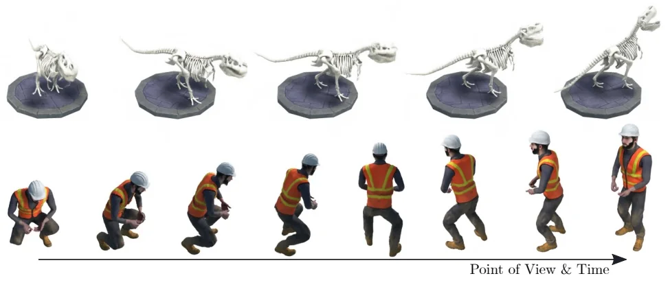
Problem Setup
The problem considered by D-NeRF is illustrated in the below figure. Given a sparse set of images of a non-rigid dynamic scene captured by a moving monocular camera, the objective is to implicitly encode the scene such that novel views at arbitrary times can be synthesized. Formally, the model must learn a mapping \[ M: ( \mathbf {x}, \mathbf {d}, t ) \mapsto ( \mathbf {c}, \sigma ), \] where \(\mathbf {x} \in \mathbb {R}^3\) is a 3D point, \(\mathbf {d}\) is the viewing direction, \(t\) is a time parameter, \(\mathbf {c} \in \mathbb {R}^3\) is the emitted color, and \(\sigma \in \mathbb {R}_{\geq 0}\) is the volume density.
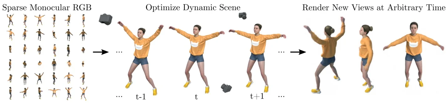
Challenges of direct spatio-temporal regression. A straightforward idea might be to extend NeRF by regressing color and density directly from both space and time, \[ M : (\mathbf {x}, \mathbf {d}, t) \mapsto (\mathbf {c}, \sigma ). \] Yet this formulation quickly breaks down: a surface point that moves or deforms across frames is assigned different coordinates at each time \(t\), and the model has no way of knowing that these correspond to the same physical entity. As a result, temporal redundancy is ignored, leading to blurred reconstructions and unstable geometry.
To address this, D-NeRF introduces an intermediate canonical configuration that serves as a shared reference for all time instants. Instead of relearning radiance for every frame, the model learns a deformation field that warps observed points back to the canonical space. Radiance and density are then predicted only once in this space, ensuring that appearance remains consistent over time.
This decomposition has clear benefits:
This design reflects how humans perceive motion: despite deformations, objects are recognized as consistent entities by mentally aligning them to an internal reference. Analogously, D-NeRF aligns all observations to its canonical configuration, laying the foundation for the method described next.
Method
The D-NeRF method generalizes NeRF to handle dynamic, non-rigid scenes by decomposing the mapping \[ M : (\mathbf {x}, \mathbf {d}, t) \mapsto (\mathbf {c}, \sigma ) \] into two learnable modules:
The resulting architecture, as can be seen in the following figure, learns how geometry changes over time via \(\Psi _t\) while maintaining appearance consistency through \(\Psi _x\).
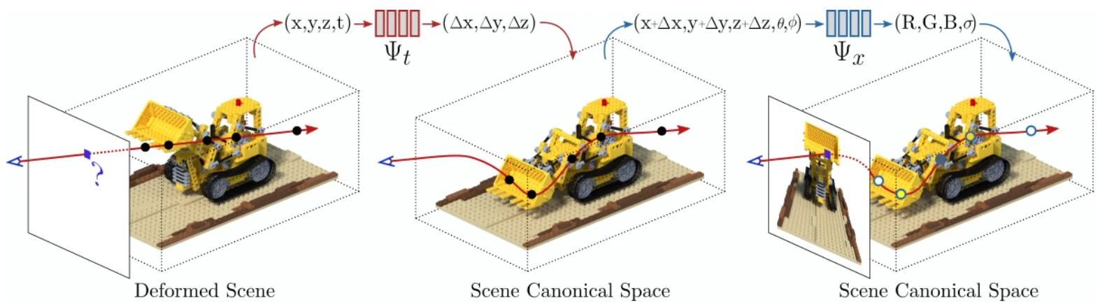
Canonical network The canonical network \(\Psi _x\) learns to represent the scene at a fixed reference state, chosen as \(t=0\). It predicts color \(\mathbf {c}\) and density \(\sigma \) for each canonical point and viewing direction: \[ \Psi _x : (\mathbf {x} + \Delta \mathbf {x}, \mathbf {d}) \mapsto (\mathbf {c}, \sigma ). \] This canonical anchor integrates information from all time instants, so that missing or occluded details in one frame can be inferred from others. Intuitively, \(\Psi _x\) functions as a static NeRF defined in canonical space, ensuring that geometry and appearance remain temporally consistent.
Deformation network The deformation network \(\Psi _t\) estimates a displacement field that maps points observed at time \(t\) into the canonical configuration: \[ \Psi _t : (\mathbf {x}, t) \mapsto \Delta \mathbf {x}, \] so that the canonical coordinate is given by \(\mathbf {x} + \Delta \mathbf {x}\). Formally, the network is constrained as \[ \Psi _t(\mathbf {x}, 0) = 0, \] ensuring that the canonical state coincides with the scene at \(t=0\). Dynamic regions (such as moving limbs or bouncing balls) receive non-zero displacements, while static background points map (hopefully) to themselves. This separation of deformation from radiance allows the canonical network to remain agnostic to motion.
Volume rendering with deformations To render an image, D-NeRF adapts the NeRF volume rendering equation to account for canonical warping. Given a ray defined by origin \(\mathbf {o}\) and direction \(\mathbf {d}\), a 3D point along the ray is \(\mathbf {x}(h) = \mathbf {o} + h\mathbf {d}\). The color of a pixel \(p\) at time \(t\) is computed as \begin {equation} C(p, t) = \int _{h_n}^{h_f} T(h, t)\,\sigma (\mathbf {p}(h,t))\,\mathbf {c}(\mathbf {p}(h,t), \mathbf {d}) \, \mathrm {d}h, \label {eq:chapter23_dnerf_volint} \end {equation} where \begin {align} \mathbf {p}(h,t) &= \mathbf {x}(h) + \Psi _t(\mathbf {x}(h), t), \label {eq:chapter23_dnerf_warp} \\ [\mathbf {c}(\mathbf {p}(h,t), \mathbf {d}), \, \sigma (\mathbf {p}(h,t))] &= \Psi _x(\mathbf {p}(h,t), \mathbf {d}), \label {eq:chapter23_dnerf_canonical}\\ T(h,t) &= \exp \!\left (-\int _{h_n}^{h} \sigma (\mathbf {p}(s,t)) \, \mathrm {d}s\right ). \label {eq:chapter23_dnerf_transmittance} \end {align}
Here \(\mathbf {p}(h,t)\) is the warped canonical point corresponding to \(\mathbf {x}(h)\), and \(T(h,t)\) is the accumulated transmittance probability along the ray. Equations 23.60–[ref] mirror NeRF’s rendering formulation, but crucially, density and radiance are queried in canonical space.
For practical training, the integrals are approximated using stratified quadrature with \(N\) samples along each ray. The discrete approximation is \begin {equation} C'(p, t) = \sum _{n=1}^{N} T'(h_n, t)\,\alpha (h_n, t, \delta _n)\,\mathbf {c}(\mathbf {p}(h_n,t), \mathbf {d}), \label {eq:chapter23_dnerf_discrete} \end {equation} with \begin {align} \alpha (h, t, \delta ) &= 1 - \exp \!\left (-\sigma (\mathbf {p}(h,t)) \,\delta \right ), \label {eq:chapter23_dnerf_alpha}\\ T'(h_n, t) &= \exp \!\left (-\sum _{m=1}^{n-1} \sigma (\mathbf {p}(h_m,t))\,\delta _m\right ), \label {eq:chapter23_dnerf_Tprime} \end {align}
where \(\delta _n = h_{n+1}-h_n\) is the distance between samples.
Learning objective The networks \(\Psi _x\) and \(\Psi _t\) are trained jointly by minimizing the mean squared error between rendered pixels and ground-truth images: \begin {equation} \mathcal {L} = \frac {1}{N_s} \sum _{i=1}^{N_s} \big \| \hat {\mathbf {C}}(p_i, t) - C'(p_i, t) \big \|_2^2, \label {eq:chapter23_dnerf_loss} \end {equation} where \(N_s\) rays are sampled per batch, \(\hat {\mathbf {C}}\) denotes the ground-truth pixel colors, and \(C'\) is the predicted color from Eq. 23.61. This supervision requires only monocular images with known camera poses, without multi-view consistency or 3D ground truth.
Architecture and Implementation Details
Network design Both the canonical network \(\Psi _x\) and the deformation network \(\Psi _t\) are implemented as multilayer perceptrons (MLPs) with eight fully connected layers of 256 units each and ReLU activations. The canonical network outputs color \(\mathbf {c}\) and density \(\sigma \) with a final sigmoid activation to constrain values to valid ranges, while the deformation network outputs displacement vectors \(\Delta \mathbf {x}\) with no final non-linearity. This separation ensures that the canonical branch specializes in appearance and geometry, while the deformation branch is free to model continuous spatial displacements.
Positional encoding As in NeRF [442], D-NeRF does not feed raw coordinates and viewing directions directly into the networks. Instead, each scalar input \(p\) is mapped to a higher-dimensional Fourier feature space: \[ \gamma (p) = \left ( \sin (2^0 \pi p), \cos (2^0 \pi p), \ldots , \sin (2^L \pi p), \cos (2^L \pi p) \right ). \] This positional encoding enables the MLPs to represent highly oscillatory functions, which is crucial for capturing fine geometric detail and sharp appearance boundaries.
D-NeRF applies the encoding separately to spatial coordinates \(\mathbf {x}\), viewing directions \(\mathbf {d}\), and time \(t\), but with different frequency depths \(L\). Spatial coordinates require high-frequency capacity to model detailed surfaces and textures, so \(L=10\) is used. By contrast, time and viewing direction are more smoothly varying quantities—motions are continuous and shading changes gradually—so a smaller frequency budget (\(L=4\)) suffices. This allocation balances expressivity and stability, ensuring the model can capture fine spatial details without overfitting to noise in temporal or directional variation.
Canonical reference frame The canonical configuration serves as a temporal anchor for the entire dynamic scene. Without loss of generality, D-NeRF defines the frame at \(t=0\) as canonical, imposing the constraint \[ \Psi _t(\mathbf {x}, 0) = 0. \] This choice is practical: one reference frame must be selected, and picking the first observed frame avoids ambiguity while ensuring that the deformation network only learns displacements for \(t \neq 0\). Anchoring to \(t=0\) guarantees that all temporal states are consistently mapped to a single geometry, so that the canonical network \(\Psi _x\) always operates in a stable coordinate system.
Curriculum strategy Training D-NeRF directly on the full temporal range is challenging, since large deformations between distant time instants make optimization unstable. To mitigate this, the authors introduce a curriculum learning strategy: input frames are ordered chronologically and introduced gradually, starting from those close to the canonical frame and progressively extending to more distant time instants. This approach allows the networks to first master small deformations, then progressively handle larger ones. The effect is similar to learning a language by starting with simple phrases before moving to complex sentences—by staging the difficulty, convergence is improved and the learned deformation fields remain smoother and more coherent.
Optimization details Training is conducted on \(400\times 400\) images for 800k iterations. Each batch samples \(N_s = 4096\) rays, with 64 samples per ray. The Adam optimizer [305] is used with initial learning rate \(5\!\times \!10^{-4}\), exponential decay to \(5\!\times \!10^{-5}\), and momentum parameters \(\beta _1=0.9\), \(\beta _2=0.999\). On a single Nvidia GTX 1080 GPU, training takes approximately two days.
Experiments and Ablations
D-NeRF is evaluated on a dataset of eight synthetic dynamic scenes rendered with complex motions and non-Lambertian materials. Each sequence contains between 100 and 200 frames at \(800\times 800\) resolution, with ground-truth train/validation/test splits. The experiments aim to dissect the contributions of the canonical and deformation networks, and to compare D-NeRF against two alternatives:
Learned canonical scene and displacement fields D-NeRF successfully learns a displacement field \(\Delta \mathbf {x}\) that aligns all observations to a sharp canonical space. The following figure illustrates this mapping: dynamic inputs at different time instants are warped into the canonical configuration, where geometry and appearance remain stable. The figure shows radiance rendering, density mesh, depth map, and color-coded correspondences. Matching colors across canonical and deformed meshes demonstrate that temporal correspondences are preserved, even though each deformation state is only seen from a single viewpoint.
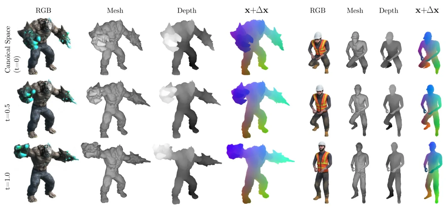
Shading and appearance consistency A key challenge is handling shading effects and appearance changes over time. The following figure shows a scene with three balls made of plastic (green), translucent glass (blue), and metal (red). Although shadows and highlights move across the floor as objects deform, D-NeRF encodes these changes by warping the canonical configuration. For instance, shadows cast by the red ball at \(t=0.5\) and \(t=1\) are aligned to different canonical regions, yet the network synthesizes them consistently. This demonstrates that D-NeRF can separate geometry from shading variation, producing coherent results without explicitly modeling illumination.
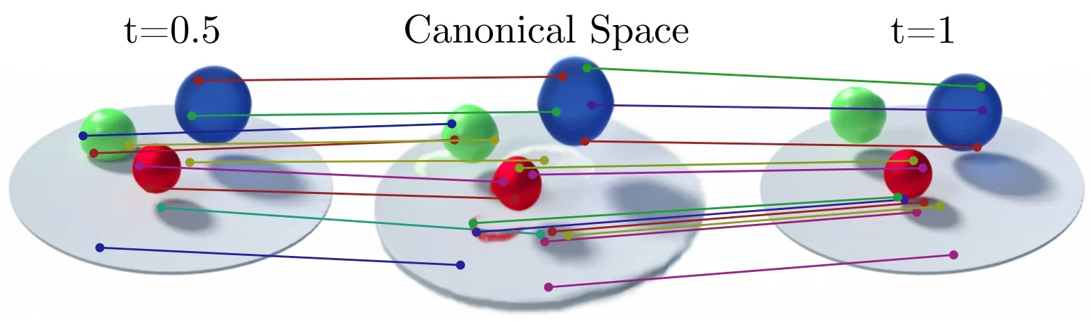
Quantitative and qualitative comparisons D-NeRF is compared against two baselines:
As shown in the following table, D-NeRF consistently outperforms both baselines across metrics including MSE, PSNR, SSIM, and LPIPS. Qualitatively, NeRF collapses to blurry averages of motion, while T-NeRF captures coarse dynamics but fails on high-frequency details such as textures and fine structures. D-NeRF preserves sharpness and reproduces fine detail, despite each time instant being observed from only a single camera.
Hell Warrior | Mutant | Hook | Bouncing Balls |
|||||||||||||
|---|---|---|---|---|---|---|---|---|---|---|---|---|---|---|---|---|
| Method | MSE\(\downarrow \) | PSNR\(\uparrow \) | SSIM\(\uparrow \) | LPIPS\(\downarrow \) | MSE\(\downarrow \) | PSNR\(\uparrow \) | SSIM\(\uparrow \) | LPIPS\(\downarrow \) | MSE\(\downarrow \) | PSNR\(\uparrow \) | SSIM\(\uparrow \) | LPIPS\(\downarrow \) | MSE\(\downarrow \) | PSNR\(\uparrow \) | SSIM\(\uparrow \) | LPIPS\(\downarrow \) |
| NeRF [37] | 44e-3 | 13.52 | 0.81 | 0.25 | 9e-4 | 20.31 | 0.91 | 0.09 | 21e-3 | 16.65 | 0.84 | 0.19 | 1e-2 | 18.28 | 0.88 | 0.23 |
| T-NeRF (temporal baseline) | 47e-4 | 23.19 | 0.93 | 0.08 | 8e-4 | 30.56 | 0.96 | 0.04 | 18e-4 | 27.21 | 0.94 | 0.06 | 6e-4 | 32.01 | 0.97 | 0.04 |
| D-NeRF [48] | 31e-4 | 25.02 | 0.95 | 0.06 | 7e-4 | 31.29 | 0.97 | 0.02 | 11e-4 | 29.25 | 0.96 | 0.11 | 5e-4 | 32.80 | 0.98 | 0.03 |
Lego | T-Rex | Stand Up | Jumping Jacks |
|||||||||||||
| Method | MSE\(\downarrow \) | PSNR\(\uparrow \) | SSIM\(\uparrow \) | LPIPS\(\downarrow \) | MSE\(\downarrow \) | PSNR\(\uparrow \) | SSIM\(\uparrow \) | LPIPS\(\downarrow \) | MSE\(\downarrow \) | PSNR\(\uparrow \) | SSIM\(\uparrow \) | LPIPS\(\downarrow \) | MSE\(\downarrow \) | PSNR\(\uparrow \) | SSIM\(\uparrow \) | LPIPS\(\downarrow \) |
| NeRF [37] | 9e-4 | 20.30 | 0.79 | 0.23 | 3e-3 | 24.49 | 0.93 | 0.13 | 1e-2 | 18.19 | 0.89 | 0.14 | 1e-2 | 18.28 | 0.88 | 0.23 |
| T-NeRF (temporal baseline) | 3e-4 | 23.82 | 0.90 | 0.15 | 9e-4 | 30.19 | 0.96 | 0.13 | 7e-4 | 31.24 | 0.97 | 0.02 | 6e-4 | 32.01 | 0.97 | 0.03 |
| D-NeRF [48] | 6e-4 | 21.64 | 0.83 | 0.16 | 6e-4 | 31.75 | 0.97 | 0.03 | 5e-4 | 32.79 | 0.98 | 0.02 | 5e-4 | 32.80 | 0.98 | 0.03 |
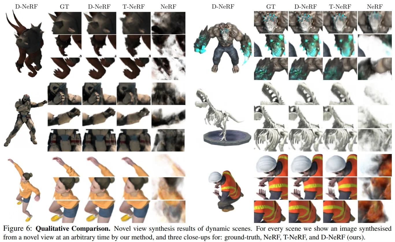
Time and view conditioning Finally, D-NeRF demonstrates robust novel-view synthesis across both space and time. The following figure shows renderings of diverse dynamic scenes from novel viewpoints at multiple time instants. The first column displays the canonical configuration, while subsequent columns show warped renderings across time. The model generalizes to articulated human motion, asynchronous object motion, and complex deformations. Interestingly, even when the canonical space appears slightly blurry (as in the Jumping Jacks scene), the warped renderings remain sharp, indicating that the deformation field compensates to maximize rendering quality.
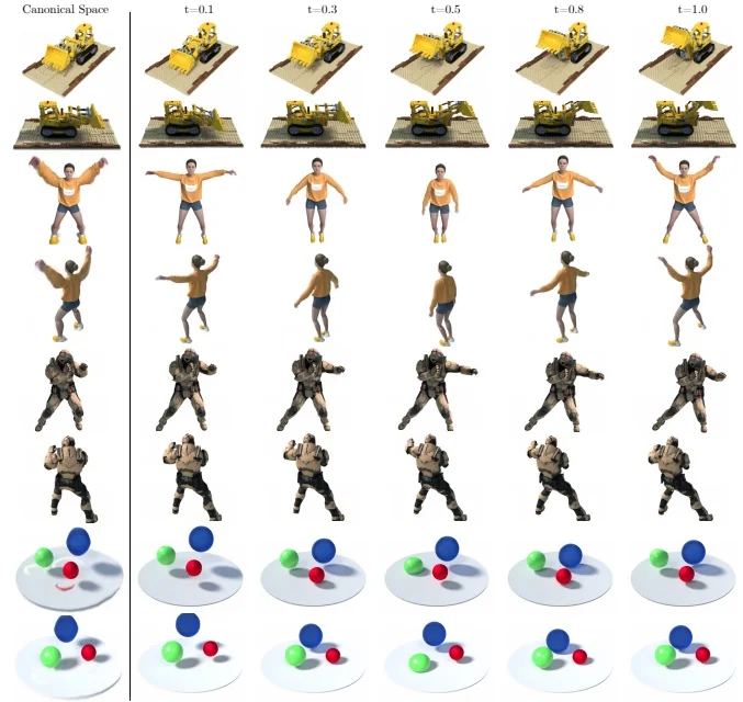
Limitations Although D-NeRF represents an important step beyond static NeRF by explicitly modeling dynamics through a canonical scene representation and a time-conditioned deformation network, it still exhibits several notable limitations:
Future directions These limitations motivated a wave of follow-up research that sought to make dynamic NeRFs more practical and robust:
In summary, D-NeRF established the usefulness of canonicalization for dynamic scene reconstruction but remained limited by its computational demands, reliance on synthetic settings, and difficulty with complex deformations. The next method we examine, Nerfies, was developed precisely to address these shortcomings, adapting the canonical–deformation formulation to casually captured real-world videos.
Enrichment 23.12.4: Nerfies: Deformable Neural Radiance Fields
Motivation
Dynamic NeRFs such as D-NeRF [502] demonstrated that a canonical radiance field plus a deformation mechanism can reconstruct non-rigid scenes; however, D-NeRF was validated primarily on synthetic data with known calibration and dense coverage. Nerfies [483] adapts this canonical–deformation paradigm to casual, real-world captures (handheld mobile selfies), introducing design choices to handle photometric inconsistency, large yet locally rigid motion, and under-constrained optimization. The goal of the work is photorealistic, free-viewpoint renderings of people and everyday scenes captured outside controlled rigs.
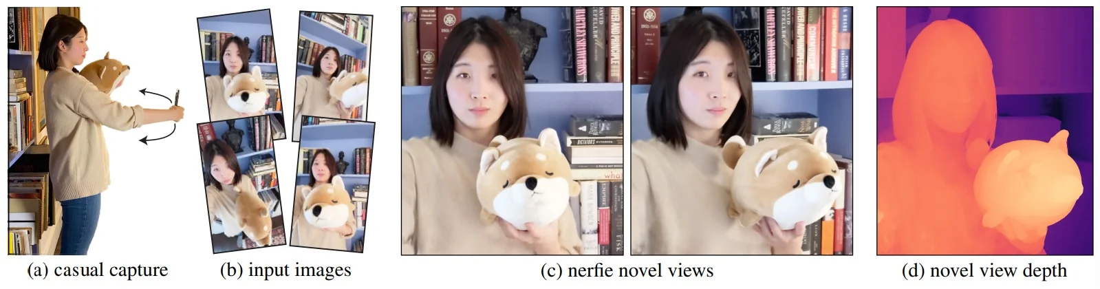
Method
Nerfies retains a canonical radiance field but replaces time-conditioned displacements with per-image latent–conditioned \(\mathrm {SE}(3)\) deformation fields, stabilized by elastic regularization and a coarse-to-fine (c2f) schedule on positional encodings. Compared to D-NeRF’s \( (\mathbf {x},t)\mapsto \Delta \mathbf {x} \), this design introduces the following key shifts:
Motivation relative to D-NeRF While D-NeRF established the value of canonicalization for dynamic scenes, its reliance on synthetic data and time-conditioned displacements limited applicability to real-world captures. Nerfies adapts the same blueprint to unconstrained videos, focusing on robustness to casual data collection, realistic motion modeling, and training stability. In doing so, it addresses D-NeRF’s key weaknesses—pose anchoring, rotational ambiguity, and fragile optimization—while preserving the benefits of a canonical template
Canonical radiance field A canonical NeRF \[ F:(\mathbf {x}',\mathbf {d},\psi _i)\;\mapsto \;(\mathbf {c},\sigma ) \] maps canonical 3D position \(\mathbf {x}'\), view direction \(\mathbf {d}\), and an appearance latent \(\psi _i\) to color and density. The use of per-image appearance latents follows the idea introduced in NeRF-W (see Enrichment Enrichment 23.11.1), where such codes compensate for photometric variations across casually captured images (e.g., exposure, white balance, or tone mapping). This differs from D-NeRF, where the canonical template is tied to the frame at \(t{=}0\), effectively anchoring the scene to an arbitrary temporal reference. In Nerfies, the canonical radiance field instead represents a learned, temporally invariant template of the subject, disentangled from both time and observation-specific appearance. The canonical configuration is not selected from a single frame but is optimized jointly during training so that all deformed observations can be consistently mapped into it.
Observation-to-canonical deformation Each input image \(i\) is associated with two learned latents: an appearance code \(\psi _i\) (as in NeRF-W; see Enrichment Enrichment 23.11.1) that absorbs photometric variations, and a deformation code \(\omega _i\) that indexes a per-image deformation field. For a sample \(\mathbf {x}\) on a camera ray in the observation frame, \[ T:(\mathbf {x},\omega _i)\;\mapsto \;\mathbf {x}' \,, \qquad G(\mathbf {x},\mathbf {d},\psi _i,\omega _i) \;=\; F\!\big (T(\mathbf {x},\omega _i),\,\mathbf {d},\,\psi _i\big ). \] Rendering proceeds by sampling along the ray in the observation frame, mapping samples to the canonical frame via \(T\), querying the canonical field \(F\), and volumetrically integrating as in NeRF.
Relation to D-NeRF. D-NeRF ties deformation to an explicit time index \(t\), which implicitly anchors the canonical to a particular frame and encourages frame-tracking warps. Nerfies instead replaces \(t\) with per-image deformation indices \(\omega _i\) and learns the canonical jointly with \(F\) and \(T\). This shift has several practical consequences:
Inference for new views (same scene). During training, each input image is assigned two codes: a deformation code \(\omega _i\) (capturing the pose or state of the scene in that frame) and an appearance code \(\psi _i\) (capturing its photometric style, e.g., exposure). Once training is complete, we can render the scene from any new camera without retraining:
In short, Nerfies inference works by treating each frame’s latent codes as a handle on the scene’s configuration. By reusing or interpolating these codes, the model can render captured or novel states from arbitrary viewpoints, and with arbitrary appearance settings, something that time-anchored methods like D-NeRF cannot easily achieve.
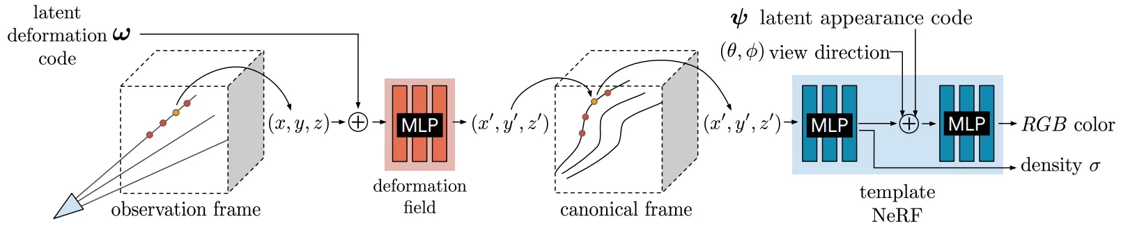
Why dense \(\mathrm {SE}(3)\) fields A naive displacement field writes \(\mathbf {x}'=\mathbf {x}+V(\mathbf {x},\omega _i)\). While universal in principle, it is cumbersome for coherent rotations: a single rigid rotation must be approximated by spatially varying translations whose magnitudes grow with distance from the axis. This entangles motion type and spatial location, making the mapping hard to learn consistently and prone to shear-like artifacts.
Nerfies instead predicts a dense \(\mathrm {SE}(3)\) transform at each location, using a screw-axis parameterization \(S=(\mathbf {r};\mathbf {v})\in \mathbb {R}^{6}\) (the Lie algebra \(\mathfrak {se}(3)\)). Intuitively, \(\mathbf {r}\) encodes the local rotation axis and angle, and \(\mathbf {v}\) encodes the accompanying translation consistent with that rotation (a “twist”). Let \(\theta =\|\mathbf {r}\|\) be the rotation angle, and let \([\mathbf {r}]_\times \) denote the \(3{\times }3\) skew-symmetric matrix for cross products. The exponential map yields the rigid transform \[ e^{\mathbf {r}} \;=\; I \;+\; \frac {\sin \theta }{\theta }[\mathbf {r}]_\times \;+\; \frac {1-\cos \theta }{\theta ^{2}}[\mathbf {r}]_\times ^{2},\qquad G \;=\; I \;+\; \frac {1-\cos \theta }{\theta ^{2}}[\mathbf {r}]_\times \;+\; \frac {\theta -\sin \theta }{\theta ^{3}}[\mathbf {r}]_\times ^{2}, \] \[ \mathbf {x}' \;=\; e^{S}\mathbf {x} \;=\; e^{\mathbf {r}}\mathbf {x} \;+\; G\,\mathbf {v}. \] Intuition. The term \(e^{\mathbf {r}}\) rotates \(\mathbf {x}\) by angle \(\theta \) around axis \(\mathbf {r}/\theta \). The matrix \(G\) converts the “velocity” \(\mathbf {v}\) in the Lie algebra into a translation that is compatible with the rotation (so that rotation and translation form a single rigid motion). When \(\theta \to 0\), the series reduce to \(e^{\mathbf {r}}\!\approx I+[\mathbf {r}]_\times \) and \(G\!\approx I+\tfrac {1}{2}[\mathbf {r}]_\times \), smoothly recovering pure translations and infinitesimal rotations. This parameterization lets the MLP express rotations coherently (one angle shared over a region) rather than reconstructing them as inconsistent, location-dependent shifts.
The deformation network \(W:(\mathbf {x},\omega _i)\mapsto (\mathbf {r},\mathbf {v})\) is initialized near identity (small outputs for \(\mathbf {r},\mathbf {v}\)), so that \(e^{S}\!\approx I\) at the start of training. This stabilizes optimization: the model learns residual motion away from no-warp, while additional priors (elastic/background regularization and the coarse-to-fine schedule) bias solutions toward plausible, near-rigid deformations where supervision is weak.
Observation vs. canonical frames The central idea of Nerfies is to disentangle appearance from motion by mapping every observed image into a common reference. Each input frame is an observation frame—the subject in its actual pose, expression, or transient configuration at capture time. The network jointly learns a static canonical frame—a pose-agnostic 3D template—along with a deformation field that warps each observation back to this shared canonical space. The displacement vectors encode how geometry must be shifted (e.g., sideways or front–back) so that all observations reconcile into a single, consistent template.
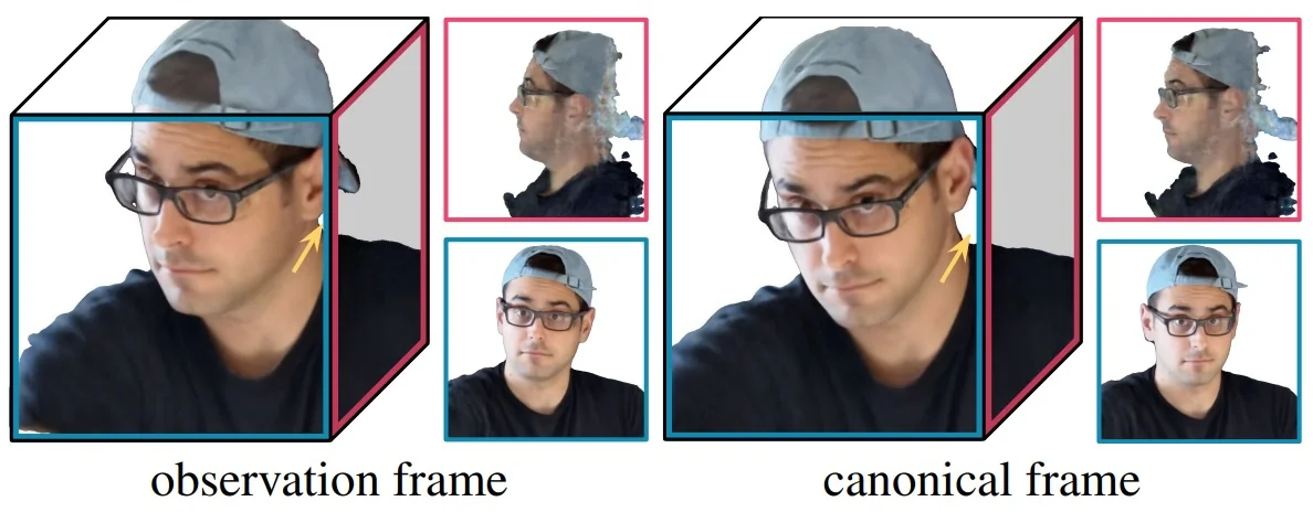
Elastic regularization (why, what, how) Why. Jointly fitting the canonical radiance field \(F\) and the deformation \(T\) from only photometric supervision is under–constrained: many different \((F,T)\) pairs can reproduce the same pixels. In practice, the optimizer may “explain” motion by letting \(T\) shrink, stretch, or shear space (degenerate but photometrically cheap), rather than by learning the intended near–rigid motion. Plain smoothness penalties (as in D-NeRF) do not directly discourage such volume changes.
What. Nerfies therefore adds an as-rigid-as-possible prior: locally, a small neighborhood should behave like a rigid body (rotation + translation), i.e., preserve lengths/areas/volumes. This explicitly targets “shrink/grow” modes.
How. Let \(J_T(\mathbf {x})=\partial T(\mathbf {x},\omega _i)/\partial \mathbf {x}\) be the Jacobian of the deformation at a sample \(\mathbf {x}\). With the SVD \(J_T=U\Sigma V^\top \) and singular values \(\{\sigma _k\}\), rigidity corresponds to \(\Sigma =I\) (no local scaling). We penalize deviation from this condition using the log-scale error \[ \mathcal {L}_{\mbox{elastic}}(\mathbf {x}) \;=\; \big \|\log \Sigma \big \|_F^2, \] where \(\log \Sigma =\mathrm {diag}(\log \sigma _1,\log \sigma _2,\log \sigma _3)\). Using \(\log \) makes expansion and contraction symmetric (e.g., \(\sigma {=}2\) and \(\sigma {=}0.5\) incur equal cost in magnitude). For robustness to truly non-rigid regions and occasional outliers, Nerfies applies a Geman–McClure penalty to the log-scale magnitude, \[ \mathcal {L}_{\mbox{elastic-r}}(\mathbf {x}) \;=\; \rho \!\left (\big \|\log \Sigma \big \|_F,\;c\right ), \] and weights the term by ray transmittance so that empty space (which should be free to warp to account for foreground motion against a static background) is not over-regularized.
Intuition in one sentence. The loss tells the network: “prefer deformations that look locally rigid (rotate/translate) and only scale when necessary,” which steers optimization away from photometrically convenient but geometrically implausible solutions that simple smoothness cannot prevent.
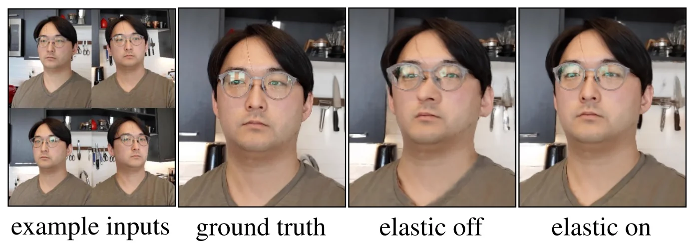
Background regularization Static points (e.g., from SfM) are softly encouraged to remain fixed in canonical space to prevent background drift: \[ \mathcal {L}_{\mbox{bg}} \;=\; \frac {1}{K}\sum _{k=1}^{K} \big \| T(\mathbf {x}_k,\omega _i) - \mathbf {x}_k \big \|_2^2. \]
Coarse-to-fine optimization (why, what, how) Why. If the deformation network can express high spatial frequencies from the start, it may overfit tiny appearance cues and settle in poor local minima before the large, global motion is discovered.
What. We therefore curriculum the capacity of the deformation MLP: begin with only low-frequency (smooth) warps, then gradually admit higher frequencies so the model first aligns the big motion and only later refines fine detail.
How. Let \(\gamma (\mathbf {x})\) denote the positional encoding of coordinates used by the deformation network \(T\). Its \(j\)-th frequency band is multiplied by a Hann window weight \[ w_j(\alpha )\;=\;\frac {1-\cos \!\big (\pi \,\mathrm {clamp}(\alpha -j,\,0,\,1)\big )}{2}, \qquad \alpha (t)\;=\;\frac {m\,t}{N}, \] where \(m\) is the maximum number of bands and \(t\!\in [0,N]\) indexes training. Early on \(\alpha \!\approx \!0\), so \(w_j(\alpha )\!\approx \!0\) for all high \(j\) and only the lowest bands are active (smooth warps). As \(t\) increases, the window slides to the right, smoothly turning on higher bands until, at \(\alpha =m\), all are fully active.
Effect. The network first solves the easy, low-frequency alignment (rigid/large motions), then safely adds high-frequency corrections (facial wrinkles, cloth folds, small non-rigid motion). This schedule consistently avoids bad minima while preserving the ability to model fine motion by the end of training.
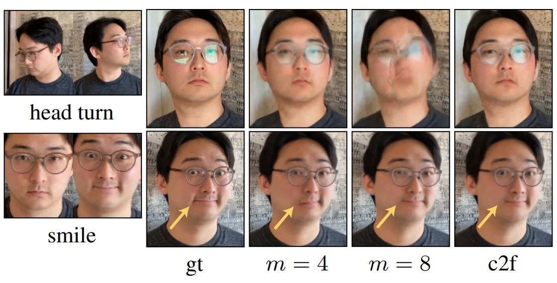
Latent-code interpolation Per-image conditioning means each training frame \(i\) carries two learned embeddings: an appearance code \(\psi _i\) and a deformation code \(\omega _i\). Because \(\omega _i\) indexes the scene state (pose/deformation) independently of camera, we can synthesize intermediate states by interpolating in the deformation-latent space while rendering from any camera: \[ \omega (\alpha ) = (1{-}\alpha )\,\omega _{\mbox{start}} + \alpha \,\omega _{\mbox{end}},\qquad \alpha \in [0,1]. \] Holding \(\psi \) fixed (or blending it similarly) produces smooth motion with consistent geometry and appearance in novel views.
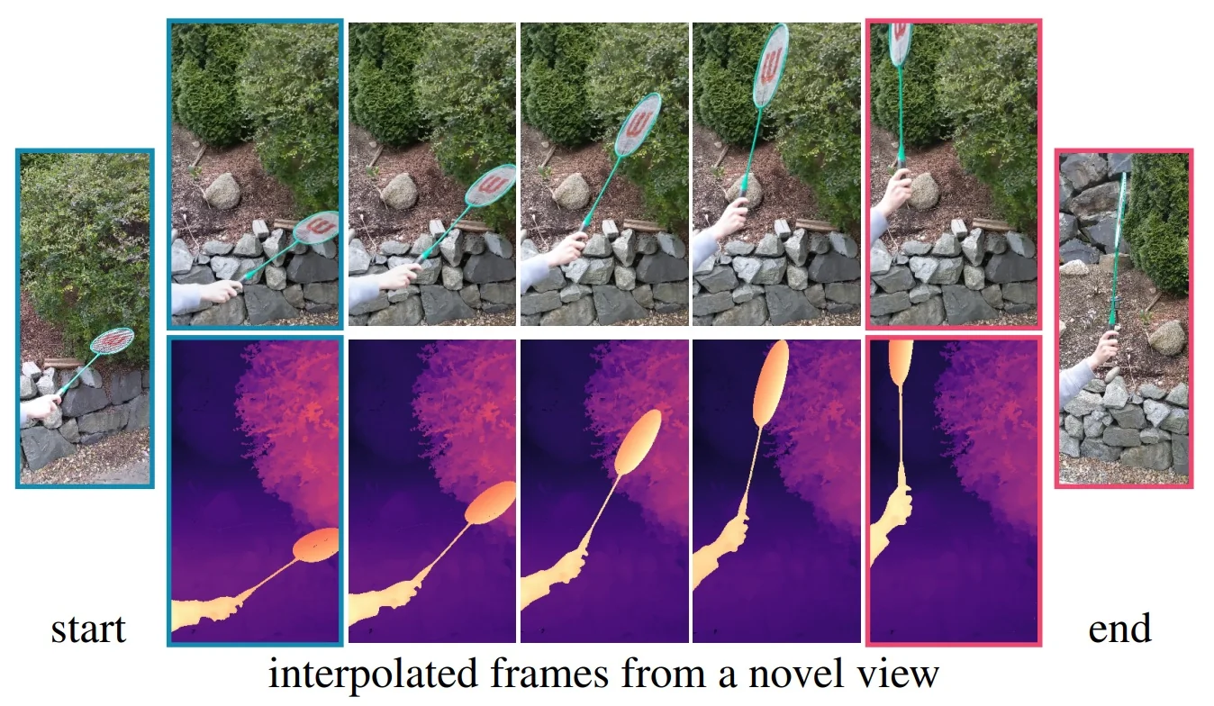
Architecture and implementation details
Canonical field. A NeRF-style MLP \(F:(\mathbf {x}',\mathbf {d},\psi _i)\!\mapsto \!(\mathbf {c},\sigma )\) with sinusoidal positional encodings predicts color and density in a canonical space; density uses a Softplus activation to ensure valid densities.
Deformation network. An MLP \(W\) predicts a dense \(\mathrm {SE}(3)\) field via screw parameters \((\mathbf {r},\mathbf {v})\) from encoded observation-space points and a per-image deformation code: \[ W:(\mathbf {x},\omega _i)\!\mapsto \!(\mathbf {r},\mathbf {v}),\qquad T(\mathbf {x},\omega _i)=e^{(\mathbf {r};\mathbf {v})}\mathbf {x}. \]
Per-image latents. Appearance latents \(\{\psi _i\}\) absorb photometric variation (exposure/white balance). Deformation latents \(\{\omega _i\}\) index the non-rigid state for each observation and enable state interpolation.
Experiments and Ablations
Evaluation uses synchronized dual-phone captures to obtain validation views of the same dynamic state. Baselines include NeRF, NeRF+latent, Neural Volumes, NSFF\(^\dagger \), and a D-NeRF–style \(\gamma (t)+\)Translation\(^\dagger \). Qualitative results show recovery of fine structures (e.g., hair strands) and full-body details; quantitative comparisons (PSNR/LPIPS) and ablations validate the contributions of \(\mathrm {SE}(3)\) deformations, elastic regularization, background constraints, and c2f.
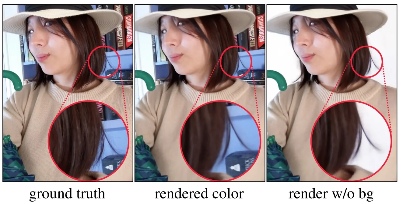
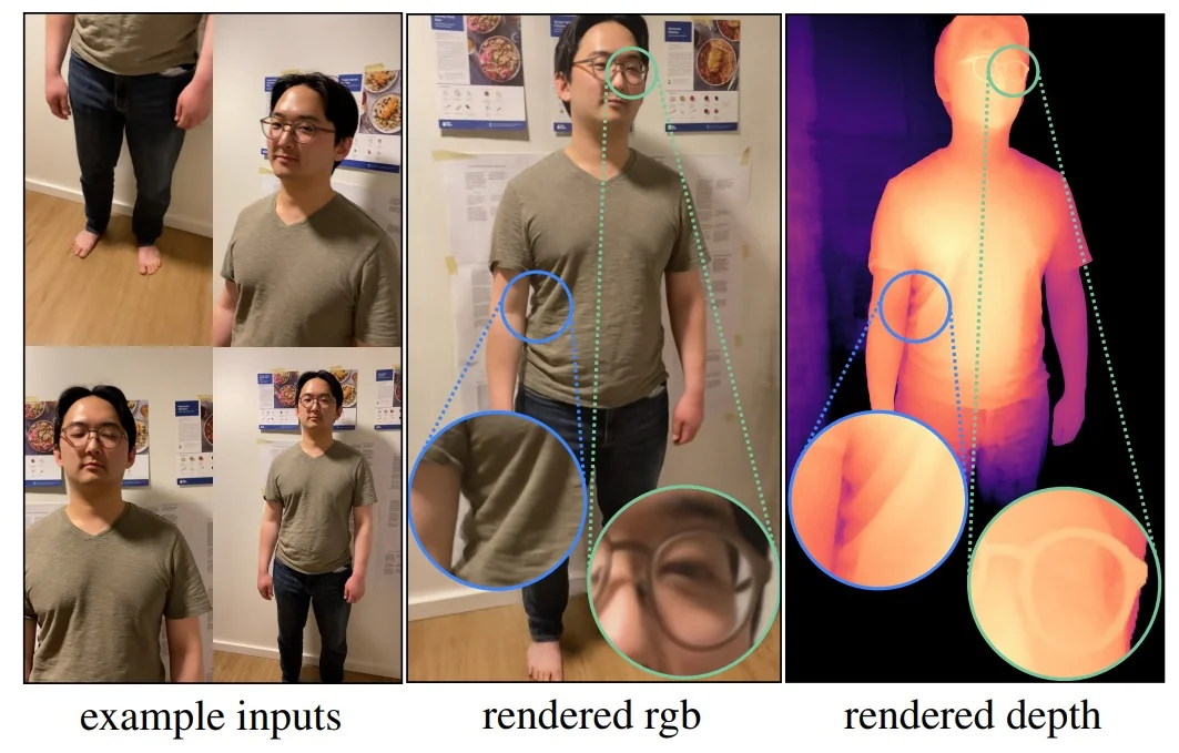
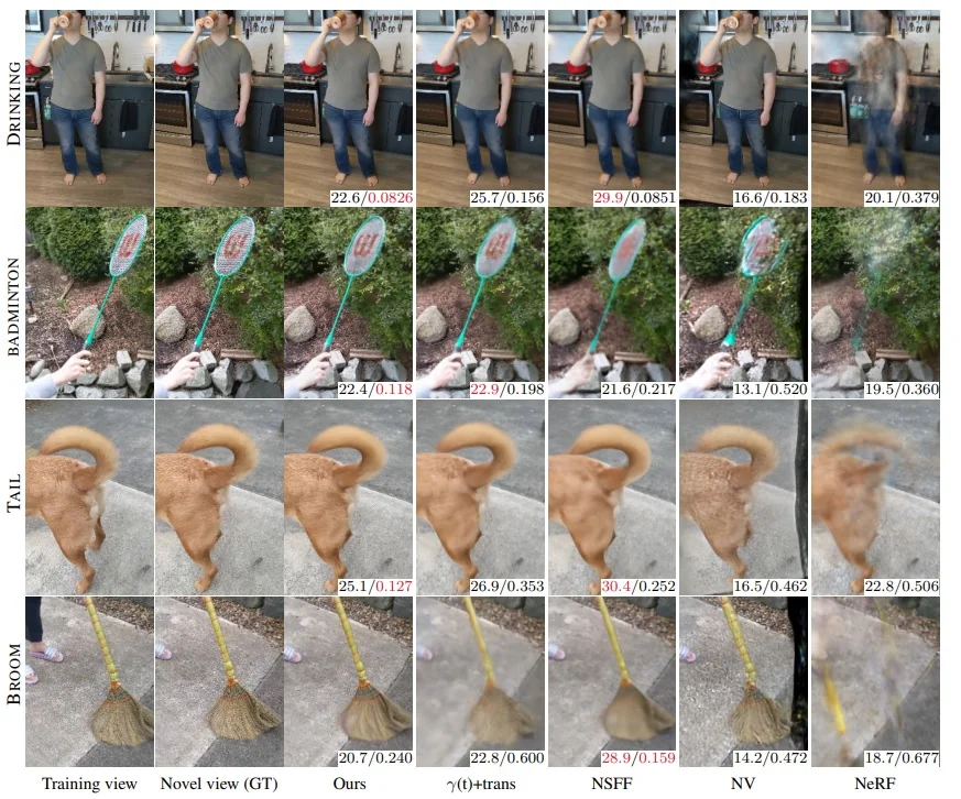
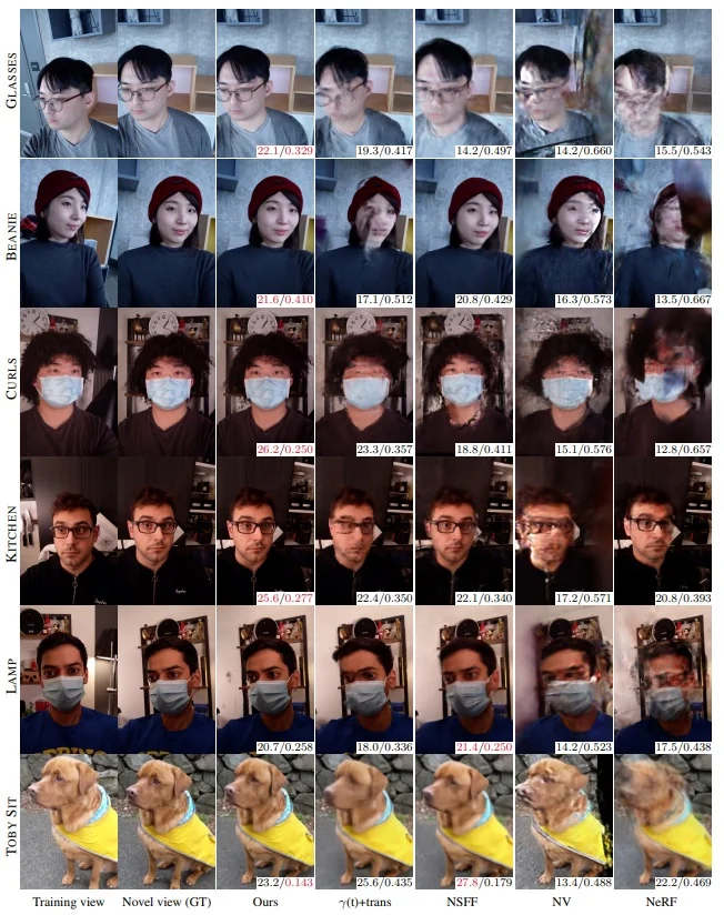
| Method | Glasses PSNR/LPIPS | Beanie PSNR/LPIPS | Curls PSNR/LPIPS | Kitchen PSNR/LPIPS | Lamp PSNR/LPIPS | Toby Sit PSNR/LPIPS | Mean PSNR/LPIPS |
| NeRF [37] | 18.10/0.474 | 16.80/0.583 | 14.40/0.616 | 19.10/0.434 | 17.40/0.444 | 22.80/0.463 | 18.10/0.502 |
| NeRF + latent | 19.50/0.463 | 19.50/0.535 | 17.30/0.539 | 20.10/0.403 | 18.90/0.386 | 19.40/0.385 | 19.10/0.452 |
| Neural Volumes [43] | 15.40/0.616 | 15.70/0.595 | 15.20/0.588 | 16.20/0.569 | 13.80/0.533 | 13.70/0.473 | 15.10/0.562 |
| NSFF\(^\dagger \) [117] | 19.60/0.407 | 21.50/0.402 | 18.00/0.432 | 21.40/0.317 | 20.50/0.239 | 26.90/0.208 | 21.30/0.334 |
| \(\gamma (t)\) + Trans\(^\dagger \) [48] | 22.20/0.354 | 20.80/0.471 | 20.07/0.426 | 22.50/0.344 | 21.90/0.283 | 25.30/0.420 | 22.20/0.383 |
| Nerfies (\(\lambda {=}0.01\)) | 23.40/0.305 | 22.20/0.391 | 24.60/0.319 | 23.90/0.280 | 23.60/0.232 | 22.90/0.159 | 23.40/0.281 |
| Nerfies (\(\lambda {=}0.001\)) | 24.20/0.307 | 23.20/0.391 | 24.90/0.312 | 23.50/0.279 | 23.70/0.230 | 22.80/0.174 | 23.70/0.282 |
| No elastic | 23.10/0.317 | 24.20/0.382 | 24.10/0.322 | 22.90/0.290 | 23.70/0.230 | 23.00/0.257 | 23.50/0.300 |
| No coarse-to-fine | 23.80/0.312 | 21.90/0.408 | 24.50/0.321 | 24.00/0.277 | 22.80/0.242 | 22.70/0.244 | 23.30/0.301 |
| No SE3 | 23.50/0.314 | 21.90/0.401 | 24.50/0.317 | 23.70/0.282 | 22.70/0.235 | 22.90/0.206 | 23.20/0.293 |
| Nerfies (base) | 24.00/0.319 | 20.90/0.466 | 23.50/0.345 | 22.40/0.323 | 22.10/0.254 | 22.70/0.184 | 22.60/0.314 |
| No BG Loss | 22.30/0.317 | 21.50/0.395 | 20.10/0.371 | 22.50/0.290 | 20.03/0.260 | 22.30/0.145 | 21.50/0.296 |
| Method | Drinking PSNR/LPIPS | Tail PSNR/LPIPS | Badminton PSNR/LPIPS | Broom PSNR/LPIPS | Mean PSNR/LPIPS |
| NeRF [37] | 18.60/0.397 | 23.00/0.571 | 18.80/0.392 | 21.00/0.667 | 20.30/0.506 |
| NeRF + latent | 21.90/0.233 | 24.90/0.404 | 20.00/0.308 | 21.90/0.576 | 22.20/0.380 |
| Neural Volumes [43] | 16.20/0.198 | 18.50/0.559 | 13.10/0.516 | 16.10/0.544 | 16.00/0.454 |
| NSFF\(^\dagger \) [117] | 27.70/0.080 | 30.60/0.245 | 21.70/0.205 | 28.20/0.202 | 27.10/0.183 |
| \(\gamma (t)\) + Trans\(^\dagger \) [48] | 23.70/0.151 | 27.20/0.391 | 22.90/0.221 | 23.40/0.627 | 24.30/0.347 |
| Nerfies (\(\lambda {=}0.01\)) | 22.40/0.087 | 23.90/0.161 | 22.40/0.130 | 21.50/0.245 | 22.50/0.156 |
| Nerfies (\(\lambda {=}0.001\)) | 21.80/0.096 | 23.60/0.175 | 22.10/0.132 | 21.00/0.270 | 22.10/0.168 |
| No elastic | 22.20/0.086 | 23.70/0.174 | 22.00/0.132 | 20.90/0.287 | 22.20/0.170 |
| No coarse-to-fine | 22.30/0.096 | 24.30/0.257 | 21.80/0.151 | 21.90/0.406 | 22.60/0.228 |
| No SE3 | 22.40/0.086 | 23.50/0.191 | 21.20/0.156 | 20.90/0.276 | 22.60/0.228 |
| Nerfies (base) | 22.60/0.127 | 24.30/0.298 | 21.10/0.173 | 22.10/0.503 | 22.50/0.275 |
| No BG Loss | 22.30/0.085 | 23.50/0.210 | 20.40/0.161 | 20.90/0.330 | 21.80/0.196 |
Limitations and Future Work
Like other diffeomorphic-warp dynamic NeRFs, Nerfies faces difficulty with genuine topology changes (e.g., mouth opening/closing) and very rapid motion, where geometry can become inconsistent despite plausible colors. This is a great limitation and a focus for future works to improve.
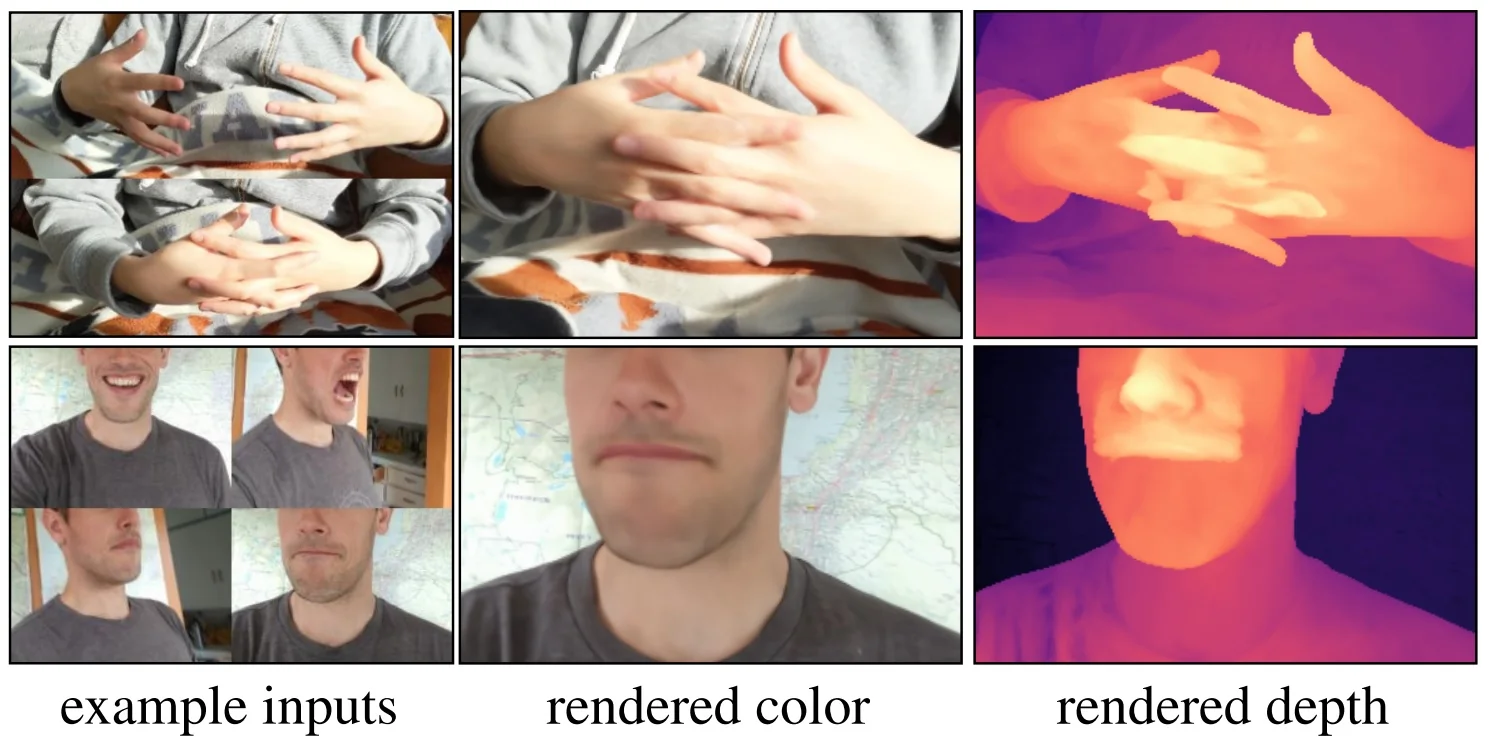
Enrichment 23.13: NeRF: Editing, Controllability & Semantic Manipulation
Decoupling geometry, appearance, and semantics enables targeted edits, retrieval, and instruction following.
Further influential works (not expanded): NeRF-Editing [167] (factorized edits via differentiable decompositions). We note broader text-guided approaches, but keep focus on language-driven interfaces directly usable for scene editing.
Enrichment 23.13.1: Language Embedded Radiance Fields (LERF)
Motivation Neural Radiance Fields (NeRFs) [442] reconstruct scenes as continuous volumetric functions, producing photorealistic novel views. Yet despite this visual fidelity, the representation itself is semantically opaque: the field encodes only colors and densities, without grounding in human-interpretable concepts. This opacity restricts interaction and control—for example, one cannot simply ask where the “utensils” are in a kitchen or identify objects based on abstract properties and affordances.
In contrast, 2D open-vocabulary methods such as LSeg [336] and OWL-ViT [446] enable language-driven reasoning about images. However, they often depend on region proposals or supervision from curated segmentation datasets, which biases generalization toward in-distribution categories and weakens expressivity for rare or long-tail queries.
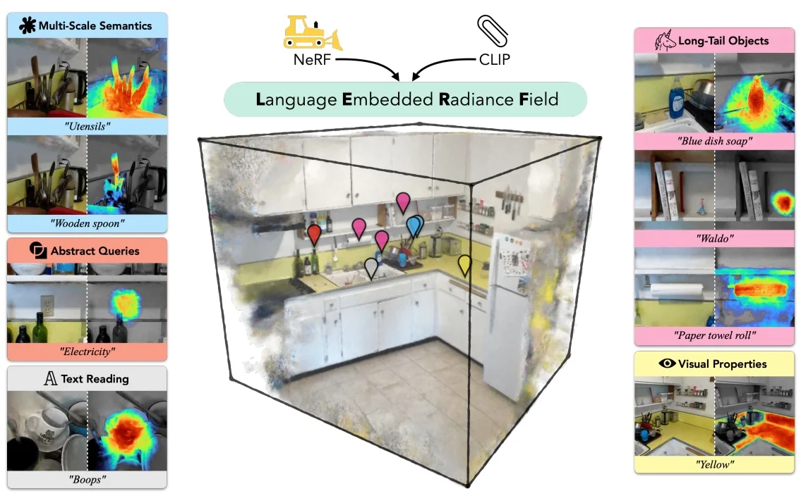
High-level overview Language Embedded Radiance Fields (LERF) [300] close the semantics gap by grounding raw CLIP [512] embeddings in a dense, multi-scale 3D field that is optimized alongside a NeRF backbone. Unlike proposal- or dataset-driven 2D pipelines, LERF does not fine-tune CLIP and does not rely on segmentation masks. The key idea is to make language supervision volumetric and scale-aware: instead of supervising infinitesimal points (ill-posed for patch-based CLIP), LERF learns a view-independent language field: \[ F_{\mbox{lang}}(\mathbf {x}, s) \in \mathbb {R}^d \] that outputs a CLIP vector for a 3D cube centered at \(\mathbf {x}\) with physical side length \(s\). Supervision comes from a precomputed multi-scale pyramid of CLIP embeddings derived from image crops of training views. During rendering, NeRF’s density weights integrate these features along rays to produce pixel-aligned, view-consistent relevancy maps for arbitrary text prompts.
Why this suits open-vocabulary 3D queries LERF transforms a static NeRF reconstruction into a semantic 3D interface that can be queried directly with natural text. Its design provides three key advantages:
In practice, these capabilities can be realized from a casual hand-held capture: a scene is reconstructed in under one hour, after which relevancy maps for arbitrary text prompts can be generated interactively in real time.
Method
The central contribution of LERF [300] is to extend the NeRF framework with a language field that grounds natural language in 3D space. Below, we detail the method from the field definition and supervision to volumetric rendering and regularization.
Language field definition Standard NeRF parameterizes a continuous volumetric function \[ F(\mathbf {x}, \mathbf {d}) \mapsto (\sigma , c), \] where each 3D sample \(\mathbf {x}\) and viewing direction \(\mathbf {d}\) yield a density \(\sigma \) and view-dependent color \(c\). This encodes only geometry and appearance, with no semantics. LERF augments this with a view-independent language field computed from a shared semantic backbone \(E_{\mbox{feat}}\): \[ \mathbf {h}(\mathbf {x}) \;=\; E_{\mbox{feat}}(\mathbf {x}), \qquad F_{\mbox{lang}}\!\big (\mathbf {h}(\mathbf {x}), s\big ) \in \mathbb {R}^{512}. \] Unlike NeRF’s infinitesimal point queries, \(F_{\mbox{lang}}\) is defined over volumes: for a cube centered at \(\mathbf {x}\) with side length \(s\), the output is a CLIP feature vector describing that region’s semantics. The explicit physical scale \(s\) is essential: large \(s\) aggregates broad context (e.g., “utensils” across a drawer), while small \(s\) isolates fine parts (e.g., a “wooden spoon”). \(F_{\mbox{lang}}\) is view-independent, so multiple views of the same 3D region reinforce a single semantic embedding.
Supervision via CLIP pyramid CLIP produces semantics for image patches with context, while NeRF samples 3D points. LERF supervises a world-space volume \((\mathbf {x}, s)\) using the CLIP embedding of the image patch onto which it projects. The pipeline: (i) precompute, for each training image, a multi-scale “textbook” of CLIP features in image coordinates; (ii) during training, project \((\mathbf {x}, s)\) into a view and read the matching embedding via interpolation.
Part 1 — Precomputation: building the image-space textbook
Part 2 — Training: supervising a world-space volume with an image-space patch
Notes on correctness and design
Volumetric language rendering The NeRF scene is trained photometrically to predict \((\sigma , c)\); this backbone is unchanged. LERF adds a parallel, view-independent semantic layer rendered with the same sampler and transmittance. Along \(\mathbf {r}(t)=\mathbf {o}+t\mathbf {d}\) with step size \(\delta _i\), opacity \(\alpha _i = 1-\exp (-\sigma _i\,\delta _i)\), and transmittance \(T_i = \prod _{j<i}(1-\alpha _j)\), \[ \hat {\varphi }_{\mbox{lang}}(u,v;s) \;=\; \sum _{i} w_i \, F_{\mbox{lang}}\!\big (\mathbf {h}(\mathbf {r}(t_i)),\, s(t_i)\big ), \qquad w_i \;=\; T_i\,\alpha _i, \] followed by \(\ell _2\) normalization. The depth-dependent \(s(t)\) mirrors the projective coupling used in supervision. Given a text query, the CLIP text encoder yields \(\varphi _{\mbox{text}}\); cosine similarity with \(\hat {\varphi }_{\mbox{lang}}\) produces a view-consistent relevancy map. During training, \[ \mathcal {L}_{\mbox{lang}} \;=\; 1 - \cos \!\Big (\,\hat {\varphi }_{\mbox{lang}}, \; \varphi ^{\mbox{CLIP}}_{\mbox{target}} \Big ), \] where \(\varphi ^{\mbox{CLIP}}_{\mbox{target}}\) is retrieved from the pyramid at the projected location and scale.
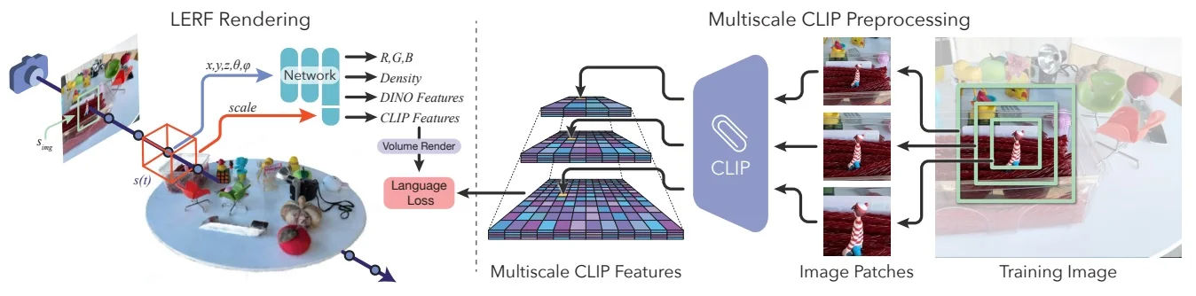
Regularization with DINO LERF augments the CLIP-driven language supervision with a second, structural head that reads the same latent features but not the scale: \[ F_{\mbox{dino}}\!\big (\mathbf {h}(\mathbf {x})\big ) \in \mathbb {R}^{d_{\mbox{dino}}}. \] Precomputation (DINO). Each training image is passed once through a frozen DINO ViT, producing dense, pixel-aligned descriptors \[ \varphi ^{\mbox{DINO}}(u,v)\in \mathbb {R}^{d_{\mbox{dino}}}\,. \] Unlike CLIP, which supplies a multi-scale pyramid of patch embeddings to supervise scale-aware semantics, DINO descriptors are already dense at the native image resolution and require no pyramid or scale interpolation. They provide local, category-agnostic cues (smooth within objects, sharp at boundaries).
Volumetric rendering and loss. Using the same transmittance weights \(w_i\) as RGB and the CLIP head, \[ \hat {\varphi }_{\mbox{dino}}(u,v) \;=\; \sum _i w_i \, F_{\mbox{dino}}\!\big (\mathbf {h}(\mathbf {r}(t_i))\big ), \qquad \mathcal {L}_{\mbox{dino}} \;=\; \big \| \hat {\varphi }_{\mbox{dino}}(u,v) - \varphi ^{\mbox{DINO}}(u,v) \big \|_2^2. \] Both \(\mathcal {L}_{\mbox{lang}}\) (patch-based, multi-scale CLIP) and \(\mathcal {L}_{\mbox{dino}}\) (dense, pixel-aligned DINO) backpropagate through their heads and into the shared backbone \(E_{\mbox{feat}}\), shaping \(\mathbf {h}(\mathbf {x})\) to be smooth on object interiors and to change sharply at boundaries. This regularizes the latent space that the CLIP head consumes, yielding crisper, less patchy semantics at inference—despite the DINO head never being matched to text at test time.
Inference: scale selection and heatmap rendering At inference time, LERF produces a text-driven heatmap indicating where a natural-language query is likely to be grounded in the 3D scene. Importantly, only the CLIP head and the NeRF rendering pipeline are used; the DINO head serves only as a training-time regularizer and is not involved at test time.
Scale selection (global per query). The CLIP head is conditioned on a physical scale parameter \(s\), which ties a 3D neighborhood in world coordinates to the patch sizes that CLIP was trained on. Because the optimal scale depends on the query (“kitchen” spans meters, while “wooden spoon” spans centimeters), LERF sweeps over a discrete set of candidate scales:
This procedure balances global and local queries: scene-level concepts favor larger \(s\), while fine-grained part queries favor smaller \(s\). Fixing a single global \(s\) per query stabilizes the visualization, though it assumes objects of interest are roughly consistent in size.
Text embeddings. For a user-specified query (e.g., “wooden spoon”), a frozen CLIP text encoder produces a unit-normalized embedding vector \[ \varphi _{\mbox{text}} \;\in \; \mathbb {R}^{512}. \] This serves as the reference against which all rendered CLIP features are compared.
Relevancy computation (CLIP + NeRF aggregation). Given a viewpoint and the chosen scale \(s\), each pixel \((u,v)\) accumulates semantic features along its camera ray: \[ \hat {\varphi }_{\mbox{lang}}(u,v;s) \;=\; \sum _i w_i\,F_{\mbox{lang}}\!\big (\mathbf {h}(\mathbf {r}(t_i)),\, s(t_i)\big ), \] where \(\mathbf {r}(t)\) is the ray, \(\mathbf {h}(\cdot )\) the shared latent features, and \[ w_i = T_i \alpha _i, \qquad \alpha _i = 1-\exp (-\sigma _i\delta _i), \qquad T_i = \prod _{j<i}(1-\alpha _j). \] These weights are identical to those used in NeRF’s RGB rendering, ensuring that semantic aggregation is geometry- and opacity-aware. The per-pixel relevancy score is then the cosine similarity: \[ \mbox{score}(u,v) \;=\; \cos \!\big (\hat {\varphi }_{\mbox{lang}}(u,v;s), \,\varphi _{\mbox{text}}\big ). \]
Refinements. Two additional steps sharpen the resulting heatmap:
Intuition. This inference process ensures that:
Architecture and factorization (overview, sharing, and why DINO helps). LERF is trained end-to-end with three cooperating modules: (1) a NeRF backbone \((\sigma ,c)\) for appearance/geometry that receives only \(\mathcal {L}_{\mbox{rgb}}\); (2) a shared feature backbone \(E_{\mbox{feat}}\) (multi-resolution hashgrid) that outputs \(\mathbf {h}(\mathbf {x})\); and (3) two disjoint semantic heads that both read \(\mathbf {h}(\mathbf {x})\): \[ \underbrace {F_{\mbox{lang}}\!\big (\mathbf {h}(\mathbf {x}),\,s\big )}_{\mbox{CLIP head}} \in \mathbb {R}^{512}, \qquad \underbrace {F_{\mbox{dino}}\!\big (\mathbf {h}(\mathbf {x})\big )}_{\mbox{DINO head}} \in \mathbb {R}^{d_{\mbox{dino}}}. \] Because \(\mathcal {L}_{\mbox{lang}}\) and \(\mathcal {L}_{\mbox{dino}}\) both update \(E_{\mbox{feat}}\), DINO’s dense, pixel-aligned supervision sculpts the shared latent space into geometry-aware features that directly benefit the CLIP head at inference.
Why DINO (and not SAM or detector/segmenter baselines).
Thus, DINO acts as an effective training-time structural regularizer on the shared backbone, while CLIP remains the sole driver of text matching at inference.
Training objective. LERF trains all of its components end-to-end from scratch on the target scene. The CLIP and DINO encoders that provide semantic supervision are frozen, but both the NeRF branch \((\sigma ,c)\) and the semantic backbone \(E_{\mbox{feat}}\) are actively optimized. The total loss is \[ \mathcal {L} \;=\; \mathcal {L}_{\mbox{rgb}} \;+\; \lambda _{\mbox{lang}}\,\mathcal {L}_{\mbox{lang}} \;+\; \lambda _{\mbox{dino}}\,\mathcal {L}_{\mbox{dino}}\,. \]
Why train jointly? If we were to freeze a separately trained NeRF and only add semantics afterwards, the semantic heads would be forced to sit on top of whatever ambiguities or artifacts the NeRF geometry contains (e.g., smoky volumes in textureless regions). By co-optimizing \(\mathcal {L}_{\mbox{rgb}}\), \(\mathcal {L}_{\mbox{lang}}\), and \(\mathcal {L}_{\mbox{dino}}\) together, the geometry and semantics co-adapt: RGB loss guarantees photometric fidelity, while the semantic losses push the backbone to place sharper boundaries and consistent features at object borders. The result is a decoupled but synergistic training process: geometry is accurate, semantics are consistent, and the final heatmaps are crisp and view-consistent.
Results and Ablations
Qualitative results LERF enables open-vocabulary, language-driven exploration of reconstructed 3D scenes. Given a text query (e.g., “coffee mug”), the model renders a relevancy heatmap that highlights the corresponding 3D region across novel views, acting as a soft segmentation without predefined categories or manual masks. Representative results show robust localization across: objects (“eggs”, “shoes”), parts (“hand”, “fingers”), attributes/materials (“wooden”, “glass”), abstract categories (“cartoon”, “bath toy”), long-tail named entities (“waldo”, “jake from adventure time”), and even text strings on book spines (“the cookie bible”). These maps remain view-consistent due to volumetric aggregation and the shared 3D geometry. (Adapted from [118].)
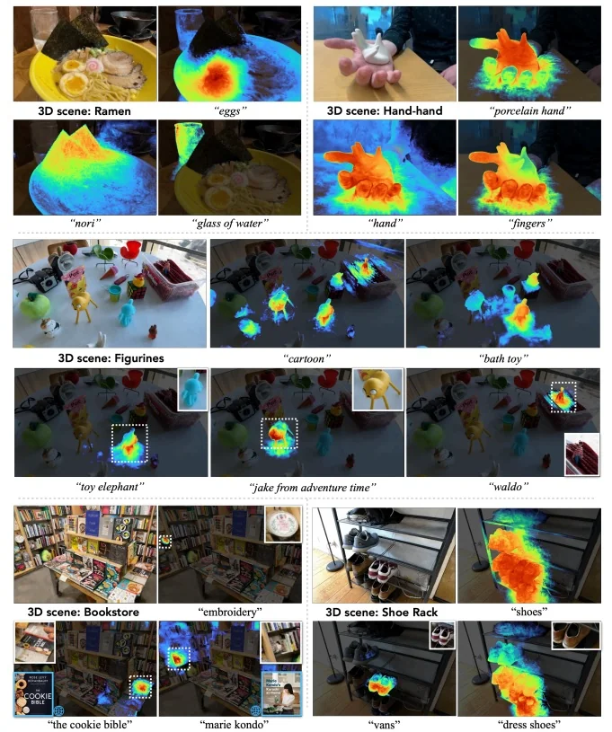
2D CLIP vs. volumetric LERF A direct 2D baseline interpolates similarity over patchwise CLIP embeddings in image space, which ignores multi-view geometry. In contrast, LERF renders language features volumetrically using NeRF transmittance, improving alignment with 3D structure.
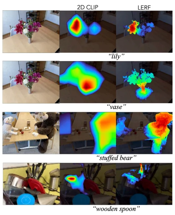
Localization against LSeg (3D) and OWL-ViT LERF is further compared to baselines that rely on 2D vision-language models projected into 3D. Results show stronger localization for long-tail concepts from novel views.
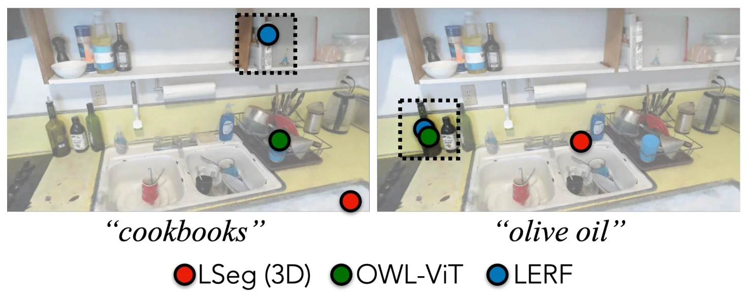
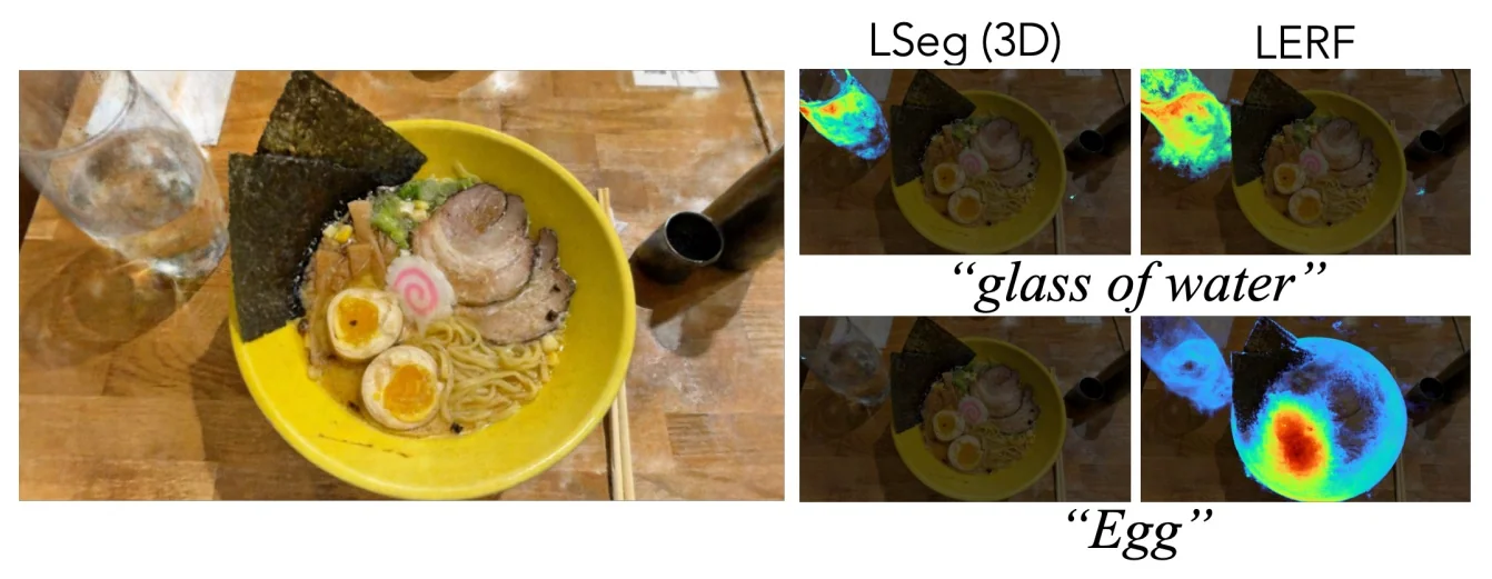
| Test Scene | LSeg (3D) | OWL-ViT | LERF |
|---|---|---|---|
| waldo kitchen | 13.0% | 42.6% | 81.5% |
| bouquet | 50.0% | 66.7% | 91.7% |
| ramen | 15.0% | 92.5% | 62.5% |
| teatime | 28.1% | 75.0% | 93.8% |
| figurines | 8.9% | 38.5% | 79.5% |
| Overall | 18.0% | 54.8% | 80.3% |
3D existence: precision–recall The task evaluates whether a queried concept exists anywhere in a scene, independently of precise localization. For each {scene, query} pair:
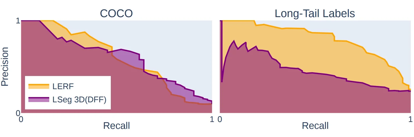
Ablation studies The contribution of DINO regularization and multi-scale CLIP supervision can be isolated through ablations. Removing DINO weakens object-level grouping and boundary sharpness, producing patchy features that bleed into the background, particularly in sparsely observed areas. Training without the CLIP pyramid (single-scale) harms both coarse context and fine parts: large objects lose global coherence and small items lose discriminative detail. Together these components regularize the shared semantic backbone and stabilize the language field across scales.
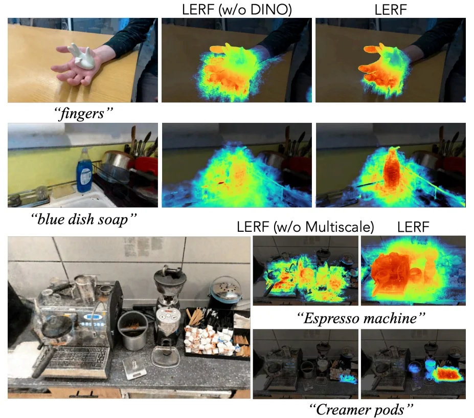
Failure cases and ambiguities Typical errors stem from (i) fine-grained category proximity in CLIP space (e.g., “zucchini” vs. other long green vegetables), (ii) visual look-alikes or texture priors (“leaf” firing on green plastic), and (iii) global context gaps where volumetric aggregation over thin structures favors edges (“table”). These issues reflect both biases in the teacher model and geometric ambiguities in under-constrained regions.
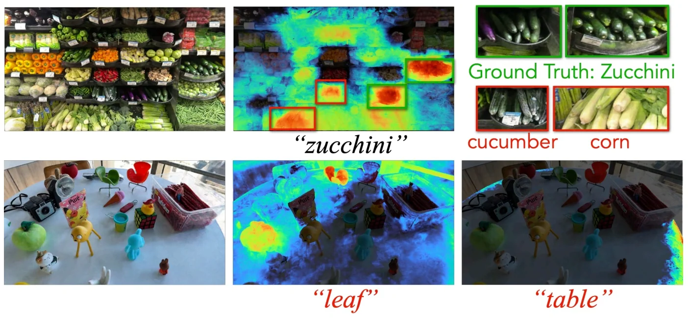
Prompt sensitivity (prompt tuning) Because CLIP embeddings are highly sensitive to text phrasing, LERF inherits this prompt sensitivity. Adding discriminative modifiers (color, material, container type) reduces ambiguity and improves accuracy, particularly when geometry is ambiguous or coverage is sparse.
CLIP bag-of-words behavior Supervision from frozen CLIP also introduces token-level quirks: compositional structure may be underweighted and nouns can dominate parts or attributes unless explicitly disambiguated. Typos that remain close in token space may also mislead supervision.
Efficiency analysis Training overhead relative to a vanilla NeRF is modest: CLIP crop pyramids and dense DINO descriptors are precomputed once per image, and training reduces to fast lookups and \(\ell _2\) regression to frozen targets. At inference, rendering language maps reuses the same rays and transmittance weights as RGB; the DINO head is inactive. Overall runtime and scaling remain comparable to standard NeRF pipelines while providing richer, open-vocabulary semantics.
Summary of findings Experimental analyses identify three design choices as critical:
Together these elements yield view-consistent, open-vocabulary 3D semantic maps that answer existence queries robustly and localize fine-grained concepts across novel viewpoints.
Enrichment 23.13.2: InstructNeRF2NeRF: Editing 3D Scenes with Instructions
Motivation
Editing implicit 3D representations is nontrivial: traditional 3D tools presuppose explicit geometry and expert workflows, whereas neural radiance fields provide no direct handles for intuitive manipulation. CLIP-guided or physics-based approaches have enabled stylization or property tweaks but often struggle with localized, instruction-driven edits that remain consistent across viewpoints. InstructNeRF2NeRF [211] proposes a language-based interface for NeRF editing by harnessing an instruction-following 2D diffusion prior and consolidating those edits into a coherent 3D scene via iterative retraining.
Background on InstructPix2Pix
The InstructNeRF2NeRF (I2N2) framework enables intuitive, language-based 3D scene editing by leveraging InstructPix2Pix (IP2P) [57], a diffusion model trained specifically for instruction-following image editing. I2N2 employs IP2P to iteratively modify the multi-view images that supervise a NeRF, thereby nudging the underlying 3D scene toward the desired text instruction. For diffusion fundamentals and classifier-free guidance, see Ch. 20, §20 and §20.
Core idea of InstructPix2Pix IP2P differs from text-to-image models by conditioning on both an input image \(c_I\) (to ground the edit) and a natural-language instruction \(c_T\) (to specify the change). Editing is performed in the latent domain by progressively denoising a noisy latent \(z_t\) toward an edited latent \(z_0\). The denoising network \(\epsilon _\theta \) predicts the injected noise, \[ \hat {\epsilon } \;=\; \epsilon _\theta \!\left (z_t;\, t,\, c_I,\, c_T\right ), \] from which the edited latent is obtained and decoded to pixels. This single-pass, dual-conditioned formulation avoids per-example inversion or fine-tuning while enabling localized, instruction-aligned edits.
Crucial controls: dual guidance scales IP2P extends classifier-free guidance with two independent scales that balance fidelity and edit strength:
Tuning \((s_I, s_T)\) is essential for multi-view consistency when IP2P is used to edit the many camera views that supervise a 3D scene.
How InstructPix2Pix is trained and why Prompt-to-Prompt alone is insufficient IP2P is trained on a large-scale instruction–edit dataset constructed synthetically [57]. Instead of hand-drawn masks, structural consistency between “original” and “edited” images is enforced at data-generation time using Prompt-to-Prompt §20 with Stable Diffusion §20: the same random seed and cross-attention structure are reused so pose, layout, and background align, and only the instructed change varies. The pipeline is:
At inference, IP2P edits real images by directly conditioning on \((c_I,c_T)\) and controlling \((s_I,s_T)\). This capability is precisely what Prompt-to-Prompt (P2P) lacks: P2P is an inference-time technique for editing images as they are generated from text, requiring the source and target prompts and access to the generation trajectory. It cannot edit arbitrary photographs because those internal states are absent. IP2P, trained on P2P-aligned pairs, learns the general skill of editing any given image from an instruction.
What IP2P brings beyond text-to-image diffusion and Prompt-to-Prompt
Connection to InstructNeRF2NeRF Text-only diffusion priors struggle on reconstructed scenes because each view would need a perfectly faithful textual description, often causing blur or divergence. InstructNeRF2NeRF (I2N2) resolves this by embedding InstructPix2Pix (IP2P) inside an Iterative Dataset Update loop that edits supervision images in the Stable-Diffusion–style latent space and then retrains the NeRF. At a high level, each cycle consists of:
Repetition consolidates potentially inconsistent per-view edits into a single, 3D-consistent solution.
Method
The core mechanism is an Iterative Dataset Update (Iterative DU) that alternates between latent-space editing of training views with InstructPix2Pix (IP2P) and NeRF optimization on the evolving dataset. Rather than modifying the NeRF loss directly with diffusion gradients, as in Score Distillation Sampling (SDS), edits are injected indirectly by refreshing the supervision images. This design retains the stability of conventional NeRF optimization while leveraging the semantic power of diffusion models.
Editing a single dataset image Given a calibrated view \(v\) with original capture \(I_v^0\), current render \(I_v^i\) from the evolving NeRF, and a global instruction \(c_T\), IP2P outputs an updated image \[ I_v^{i+1} \;\leftarrow \; U_\theta \!\big (I_v^{i},\, t;\, I_v^{0},\, c_T\big ), \] where \(U_\theta \) denotes the latent-domain editing pipeline: \[ \begin {aligned} z_{I,0} &= \mathcal {E}(I_v^0) && \mbox{(encode original capture for image conditioning } c_I),\\ z_0 &= \mathcal {E}(I_v^i) && \mbox{(encode current NeRF render)},\\ z_t &= \mbox{ForwardDiffuse}(z_0, t) && \mbox{(add noise in latent space)},\\ \hat \epsilon &= \epsilon _\theta (z_t;\, t,\, c_I{=}z_{I,0},\, c_T) && \mbox{(IP2P U-Net noise prediction with dual conditioning)},\\ \tilde z_0 &= \mbox{Denoise}(z_t,\hat \epsilon , s_I, s_T) && \mbox{(classifier-free guidance with } s_I, s_T),\\ I_v^{i+1} &= \mathcal {D}(\tilde z_0) && \mbox{(decode edited latent to RGB)}. \end {aligned} \] The noise level \(t\in [t_{\min },t_{\max }]\) trades off structure preservation (lower \(t\)) versus stronger edits (higher \(t\)).
Iterative Dataset Update At each outer iteration, the following sequence is performed:
Anchoring edits with \(I_v^0\) prevents drift across iterations, while guidance scales \((s_I,s_T)\) balance fidelity and edit strength. Repeated alternation reconciles per-view edits into a consistent 3D radiance field.
Training objective and relation to SDS The NeRF is trained with a conventional photometric reconstruction loss: \[ \mathcal {L}_{\mbox{NeRF}} \;=\; \sum _{r \in \mathcal {R}} \big \| C_\theta (r) - \hat {C}(r) \big \|_2^2, \] where \(C_\theta (r)\) is the color predicted by the NeRF for ray \(r\), and \(\hat {C}(r)\) is the RGB from the current dataset image after any IP2P updates.
This contrasts with methods that use Score Distillation Sampling (SDS), where the diffusion model provides a gradient directly on NeRF-rendered images to guide optimization toward the text prompt. While SDS can align NeRF to a description without paired data, it often yields blurry density or divergence when applied to real captures, because each camera view would require a perfectly accurate textual description.
InstructNeRF2NeRF avoids this instability by letting IP2P generate updated images that already satisfy the textual instruction. The NeRF is then trained only on image-level supervision, preserving the stability and geometric grounding of the reconstruction while still inheriting the semantic flexibility of diffusion editing.
Architecture and Implementation Details
Implementation follows nerfacto in Nerfstudio. Latent noise levels are sampled from \([t_{\min }, t_{\max }] = [0.02, 0.98]\); IP2P runs for 20 denoising steps per update. Classifier-free guidance typically uses \(s_I = 1.5\) and \(s_T = 7.5\). Each outer cycle updates one image (\(d=1\)) and performs \(n=10\) NeRF optimization steps. Training proceeds up to 30k iterations on a single Titan RTX GPU. Hyperparameters such as edit scheduling and ray sampling strategies follow the InstructNeRF2NeRF paper [211].
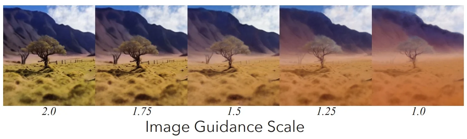
Experiments and Ablation
Qualitative edits span global scene changes (time of day, weather, material and style) and localized object or identity modifications while maintaining cross-view consistency across novel viewpoints.
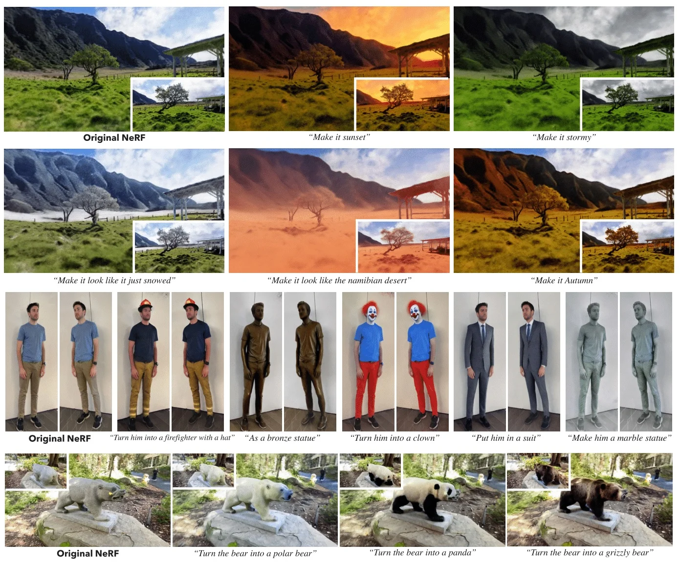
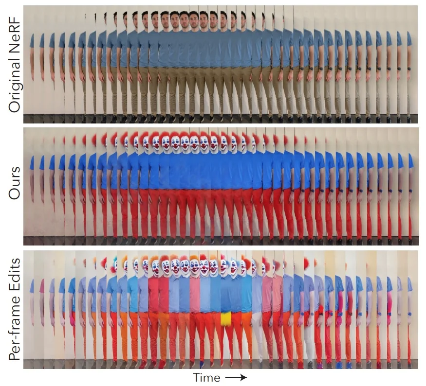
Baselines and iterative update importance The ablation suite isolates the impact of image conditioning and the iterative dataset update:
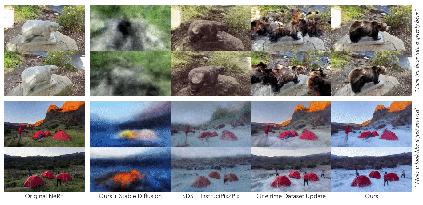
Quantitative evaluation Following the paper, two CLIP-space metrics are reported across 10 edits on two scenes: Text–image direction similarity (edit alignment) and Consistency across frames along a novel path. Results show that InstructNeRF2NeRF matches the edit strength of per-frame IP2P while achieving the best multi-view consistency.
Limitations and Future Work
Performance inherits the strengths and weaknesses of the 2D editor. When InstructPix2Pix fails to carry out the desired instruction or yields inconsistent 2D updates, consolidation into a clean 3D edit can fail. Challenging cases include large structural rearrangements, difficult removals, or subtle material edits that are under-specified.
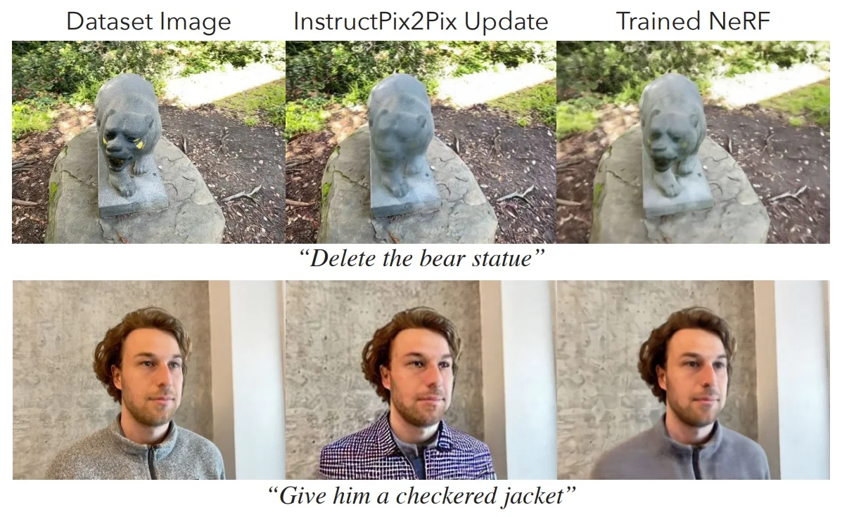
Enrichment 23.14: NeRF: Generative & Cross-Modal Foundations
Linking NeRFs with large pretrained priors (diffusion, language) enables text-to-3D and cross-modal supervision, a step toward 3D foundation models.
Further influential works (not expanded): Magic3D [361], Fantasia3D [86] (two-stage, high-res pipelines). Mentioned for context; emphasis remains on NeRF-centric generation and cross-modal supervision.
Enrichment 23.14.1: DreamFusion: Text-to-3D with Score Distillation Sampling
DreamFusion [501] tackles the ambitious goal of generating a valid 3D NeRF model directly from text, without relying on paired 3D supervision. The method’s central innovation is Score Distillation Sampling (SDS), which couples a frozen 2D diffusion model to a differentiable renderer: the diffusion prior acts as a semantic critic that supplies image-space gradients, and these are backpropagated into a NeRF to sculpt a 3D scene consistent with the text prompt.
Motivation
The aim is to produce a valid, view-consistent 3D NeRF from a single text caption, i.e., without any paired multi-view images. This problem is deeply underconstrained: many different 3D scenes can render to images that look plausible to an image-level critic at a single viewpoint. Naively optimizing photometric appearance is therefore not enough to guarantee correct geometry.
Why “many valid 2D views” need not imply valid 3D Even if each individual view looks correct, the training signal in text-to-3D is typically per-step, single-view and unpaired across time. This creates several loopholes:
Intuition (the “fog sheets” thought experiment): Think of the NeRF as controlling a cube of fog. At the start there is no object at all—the model must somehow conjure a cat from a caption. At training step \(t\), the diffusion critic looks from the front and asks for a cat. The simplest trick is to condense a thin fog sheet and paint on a flat image of a cat’s face. From the front this looks fine. At step \(t{+}1\), the critic moves to the side and again asks for a cat. Nothing forces the network to keep the same cat consistent across views: it can just create a new perpendicular fog sheet with a different painted cat profile. Each request is satisfied—the critic always sees “a cat” from its current angle—but the fog volume now contains multiple inconsistent 2D cats stitched together, not a single coherent 3D cat.
How DreamFusion closes the loophole The root problem is that many distinct 3D explanations can project to equally valid 2D images. To avoid this “per-view repainting”, DreamFusion changes the rules of rendering. Instead of allowing arbitrary view-dependent color, it splits appearance into albedo (intrinsic, view-independent surface color) and shading (appearance derived from surface normals and lighting). With this setup, the only way to make the same cat look correct from different angles is to actually form a stable 3D shape whose shading and albedo explain the critic’s feedback. Randomized camera viewpoints and lightweight view prompts bind these perspectives together, while the diffusion prior supplies semantics and realism. The result is that 2D guidance becomes not just image supervision, but a force that sculpts consistent geometry across views—even though no ground-truth 3D scene is available as in classical NeRF training.
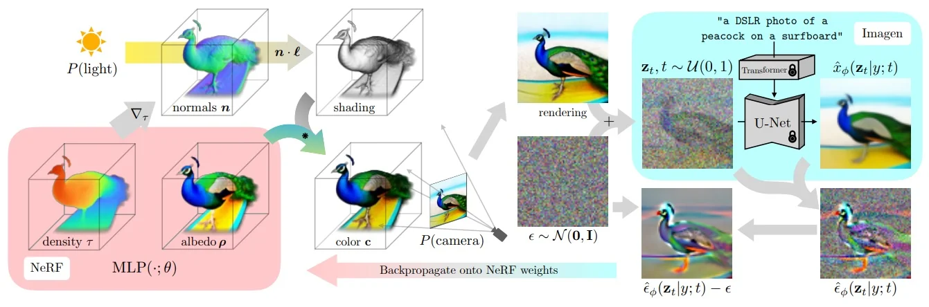
Method
High-level optimization loop At each training step DreamFusion renders an image from the current 3D field, queries a frozen diffusion prior for an image-space correction, and backpropagates that correction into the field’s parameters. The loop is:
Foreground–background separation A single NeRF that tries to explain both the object and the environment tends to take an easy shortcut: it smears low density across space or “repaints” colors per view, satisfying a 2D critic without sculpting a compact 3D shape. DreamFusion avoids this by giving the object and the environment different jobs:
The renderer combines the two with standard alpha compositing: \[ C_{\mathrm {img}} \;=\; C_{\mathrm {fg}} + (1-A)\,\mathbf {b}(\hat {\mathbf {r}}), \qquad C_{\mathrm {fg}}=\sum _i w_i\,\mathbf {c}_i,\;\; A=\sum _i w_i . \] If the object along the ray is opaque (\(A\!\approx \!1\)), the background is hidden; if the ray is empty (\(A\!\approx \!0\)), the background shows through. Trained end-to-end with SDS, the object field learns compact shape and albedo, while the background head explains the environment without inviting density “spill”. For purely scenic prompts (e.g., “a sunset”), the object field can remain nearly transparent and the background carries the content; for object-centric prompts, they cooperate naturally.
From density to orientation: making shape visible Once foreground and background are disentangled, the next step is to make the object’s geometry perceptible from a single rendered view. In images, 3D shape is revealed primarily through shading, which depends on how surfaces are oriented relative to light. To compute shading, DreamFusion derives surface orientation directly from the NeRF’s density field.
The volumetric density \(\tau (\mathbf {x})\) is a scalar field: low in empty space, high inside the object. Its gradient \(\nabla _{\mathbf {x}}\tau \) points toward the direction of steepest increase, i.e., into the solid. Flipping the sign yields an outward-pointing vector aligned with the local surface normal: \[ \mathbf {n}(\mathbf {x}) \;\propto \; -\nabla _{\mathbf {x}} \tau (\mathbf {x}), \qquad \hat {\mathbf {n}}=\frac {\sum _i w_i\,\mathbf {n}_i}{\sum _i w_i}, \] where the ray-normal \(\hat {\mathbf {n}}\) is an opacity-weighted average of sample-level normals. This construction provides the critic with orientation cues even though the NeRF never predicts normals explicitly.
With normals available, DreamFusion can introduce randomized lighting. A point light direction \(\hat {\mathbf {l}}\), ambient term \(\boldsymbol {\ell }_a\), and diffuse color \(\boldsymbol {\ell }_\rho \) define a Lambertian shading factor: \[ s_i = \boldsymbol {\ell }_a \;+\; \boldsymbol {\ell }_\rho \cdot \max \{0,\,\langle \mathbf {n}_i, \hat {\mathbf {l}}\rangle \}. \] This factor modulates albedo \(\rho _i\) at each sample to yield intensity variations that depend on surface curvature.
By alternating whether albedo is included, modulated, or removed, DreamFusion creates complementary renderings that expose different signals about appearance and shape. These become the three render modes described next, each designed to steer the critic’s gradients toward the right part of the scene representation.
Render modes: complementary recipes for supervision The object head always outputs the same raw ingredients at each 3D point: volumetric density \(\tau (\mathbf {x})\) (which sculpts shape) and albedo \(\rho (\mathbf {x})\) (the base, unlit color). From \(\tau \) we also derive a surface normal via \(-\nabla \tau \), and with a randomized light we compute a shading factor \(s\). The three render modes are not extra networks, but three different recipes for combining these ingredients into a 2D image. By showing the critic different combinations, DreamFusion exposes both texture and geometry.
Why alternate between all three? Each mode alone is insufficient. Albedo anchors colors but ignores shape; textureless shading enforces shape but discards semantics; shaded rendering mixes both but can be ambiguous about whether an error is due to color or geometry. By cycling among them, DreamFusion forces the critic’s gradients to supervise both appearance and geometry, closing off shortcuts and gradually sculpting a coherent 3D object.
This sets up the final ingredient: a way to turn the critic’s judgment into gradients. The critic is a frozen text-to-image diffusion model, and the mechanism is Score Distillation Sampling (SDS), described next.
Score Distillation Sampling: turning a 2D prior into 3D updates Goal. Use a frozen 2D diffusion model as a critic to guide a 3D NeRF. The critic never trains; only the NeRF parameters \(\theta \) are updated.
Rendering and forward noising. For a sampled camera, light, and render mode \(m\in \{\mbox{alb},\mbox{shaded},\mbox{texless}\}\), render \[ x^{(m)}(\theta )\in \mathbb {R}^{H\times W\times 3}. \] Draw timestep \(t\) and add VP noise: \[ z_t=\alpha _t\,x^{(m)}(\theta )+\sigma _t\,\varepsilon ,\qquad \varepsilon \sim \mathcal {N}(0,I),\quad \alpha _t^2+\sigma _t^2=1. \]
Frozen critic (diffusion prior). The diffusion network predicts the injected noise \[ \hat {\varepsilon }_\phi =\hat {\varepsilon }_\phi (z_t\,|\,y,t) \] (with CFG inside the call). If the render already lies on the prompt manifold, \(\hat {\varepsilon }_\phi \approx \varepsilon \); otherwise the difference \((\hat {\varepsilon }_\phi -\varepsilon )\) is a pixel-space correction.
SDS gradient (definition and derivation). DreamFusion defines the update via the critic’s score, chained through the renderer: \[ \nabla _\theta \mathcal {L}_{\mathrm {SDS}}(\theta ) =\mathbb {E}_{t,\varepsilon }\!\left [ w(t)\,\big (\hat {\varepsilon }_\phi (z_t\,|\,y,t)-\varepsilon \big )\; \frac {\partial x^{(m)}}{\partial \theta } \right ]. \] Diffusion theory gives \(\nabla _{z_t}\log p_\phi (z_t\,|\,y)\propto -(\hat {\varepsilon }_\phi -\varepsilon )/\sigma _t\), so the term \(\big (\hat {\varepsilon }_\phi -\varepsilon \big )\) is an image-space residual direction. No gradient flows through \(\hat {\varepsilon }_\phi \); all learning happens by multiplying this residual with the renderer Jacobian \(\partial x^{(m)}/\partial \theta \).
How the image residual becomes NeRF updates. Let \(G \doteq w(t)\,(\hat {\varepsilon }_\phi -\varepsilon )\in \mathbb {R}^{H\times W\times 3}\). Then \[ \nabla _\theta \mathcal {L}_{\mathrm {SDS}} = \left \langle G,\; \frac {\partial x^{(m)}}{\partial \theta } \right \rangle = \sum _{\mbox{pixels }p}\; G_p^\top \frac {\partial x^{(m)}_p}{\partial \theta }. \] For a pixel \(p\) with ray samples \(\{\mathbf {x}_i\}_{i=1}^N\), \[ C=\sum _{i=1}^N w_i\,\mathbf {c}_i,\quad A=\sum _{i=1}^N w_i,\quad w_i=T_i\,\alpha _i,\quad T_i=\prod _{j<i}(1-\alpha _j),\quad \alpha _i=1-e^{-\tau _i\,\delta _i}. \] Useful partials: \[ \frac {\partial \alpha _i}{\partial \tau _i}=\delta _i\,e^{-\tau _i\delta _i} =\delta _i(1-\alpha _i),\qquad \frac {\partial C}{\partial \rho _i}=w_i\,\mathbf {I}_3. \] We keep the standard NeRF transmittance pathway symbolic via \(\frac {\partial C}{\partial \alpha _i}\), which accounts for how changing opacity at any sample modulates all farther contributions through \(T_k\) (\(k\ge i\)).
Mode-specific decompositions. The render mode \(m\) sets \(\mathbf {c}_i\) and therefore which parameters receive strong gradients.
Albedo (unlit): appearance-centric updates \[ \mathbf {c}_i^{\mbox{alb}}=\rho _i. \] Chain rule: \[ \frac {\partial x^{\mbox{alb}}}{\partial \theta } =\sum _i \underbrace {\frac {\partial C}{\partial \rho _i}}_{w_i}\, \frac {\partial \rho _i}{\partial \theta } \;+\; \sum _i \underbrace {\frac {\partial C}{\partial \alpha _i}}_{\mbox{via }T,\;w}\, \underbrace {\frac {\partial \alpha _i}{\partial \tau _i}}_{\delta _i(1-\alpha _i)}\, \frac {\partial \tau _i}{\partial \theta }. \] Effect. The first sum (strong) refines \(\rho \) (textures/colors). The second (weaker) adjusts \(\tau \) only through transmittance—insufficient to robustly sculpt geometry on its own.
Shaded color (lit): coupled appearance\(\to \)geometry updates \[ \mathbf {c}_i^{\mbox{shaded}}=\rho _i\odot s_i,\qquad s_i=\boldsymbol {\ell }_a+\boldsymbol {\ell }_\rho \cdot \max \{0,\langle \mathbf {n}_i,\hat {\mathbf {l}}\rangle \},\quad \mathbf {n}_i \propto -\nabla _{\mathbf {x}}\tau (\mathbf {x}_i). \] Chain rule (grouping terms): \[ \frac {\partial x^{\mbox{shaded}}}{\partial \theta } =\underbrace {\sum _i \frac {\partial C}{\partial \rho _i}\frac {\partial (\rho _i\odot s_i)}{\partial \rho _i}\frac {\partial \rho _i}{\partial \theta }}_{\mbox{appearance (as in albedo)}} \;+\; \underbrace {\sum _i \frac {\partial C}{\partial \mathbf {c}_i}\frac {\partial (\rho _i\odot s_i)}{\partial \mathbf {n}_i}\frac {\partial \mathbf {n}_i}{\partial \tau _i}\frac {\partial \tau _i}{\partial \theta }}_{\mbox{geometry via normals}} \;+\; \underbrace {\sum _i \frac {\partial C}{\partial \alpha _i}\frac {\partial \alpha _i}{\partial \tau _i}\frac {\partial \tau _i}{\partial \theta }}_{\mbox{geometry via transmittance}}. \] Effect. Two geometry channels appear: (i) via normals (\(\mathbf {n}_i\propto -\nabla \tau \), which introduces derivatives of \(\nabla \tau \) w.r.t. \(\theta \); autodiff handles these), and (ii) via \(\alpha \). Shaded mode therefore sculpts \(\tau \) while still refining \(\rho \).
Textureless shaded (lit, no texture): pure geometry updates \[ \mathbf {c}_i^{\mbox{texless}}=s_i\quad (\rho \equiv \mathbf {1}). \] Chain rule: \[ \frac {\partial x^{\mbox{texless}}}{\partial \theta } =\underbrace {\sum _i \frac {\partial C}{\partial \mathbf {c}_i}\frac {\partial s_i}{\partial \mathbf {n}_i}\frac {\partial \mathbf {n}_i}{\partial \tau _i}\frac {\partial \tau _i}{\partial \theta }}_{\mbox{geometry via normals}} \;+\; \underbrace {\sum _i \frac {\partial C}{\partial \alpha _i}\frac {\partial \alpha _i}{\partial \tau _i}\frac {\partial \tau _i}{\partial \theta }}_{\mbox{geometry via transmittance}}. \] Effect. With \(\rho \) removed, all signal flows into \(\tau \). The only way to please the critic is to improve geometry (normals/curvature and occupancy).
Intuition. SDS provides a pixel-space “correction image”. The renderer’s Jacobian routes that correction into \(\rho \) in albedo mode, and into \(\tau \) (via normals and opacity) in shaded/textureless modes. Cycling the three modes resolves the classic ambiguity: albedo learns caption-faithful appearance; shaded couples appearance to curvature; textureless removes the paintbrush entirely, hardening geometry. High CFG increases realism of the supervising direction but may reduce diversity; \(w(t)\) balances contribution across noise levels.
View sampling and view-aware prompting Each iteration samples a random camera (azimuth, elevation, distance, focal multiplier) and a point light near the camera. Captions are augmented with lightweight view tokens (front/side/overhead) to align the diffusion prior’s expectations with the current viewpoint. Because albedo \(\rho \) is view-independent, variation across views must be accounted for by geometry and lighting, encouraging one coherent 3D asset rather than per-view repainting.
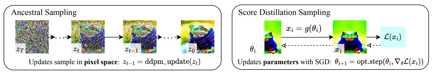
Putting the loop together Each iteration interleaves appearance- and geometry-focused signals so that SDS sculpts both \(\rho \) and \(\tau \):
Albedo steps maintain caption-faithful appearance; shaded steps sharpen geometry via normal-dependent shading; textureless steps consolidate shape by eliminating albedo as a degree of freedom. View-aware prompting stabilizes semantics across viewpoints, randomized lighting diversifies geometric cues, and background factorization prevents degenerate density fills—together converting 2D diffusion feedback into reliable, 3D-consistent supervision.
Implementation Details
Frozen diffusion prior DreamFusion employs the base Imagen model at \(64{\times }64\) with classifier-free guidance and a strong language encoder (e.g., T5-XXL). Larger guidance typically improves realism at the cost of diversity.
Foreground–background composition The object field is confined to a bounded sphere to discourage diffuse density spread. The background head provides direction-conditioned colors and is alpha-composited via transmittance, yielding object-centric assets without fog.
Experiments and Ablation
Qualitative gallery and comparisons DreamFusion produces diverse, compositionally rich assets with multi-view consistency and clean geometry.
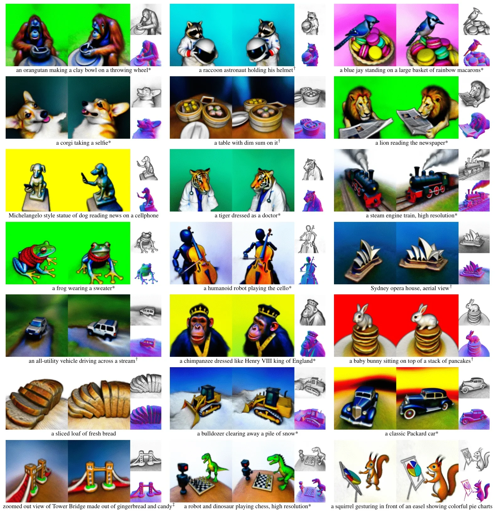
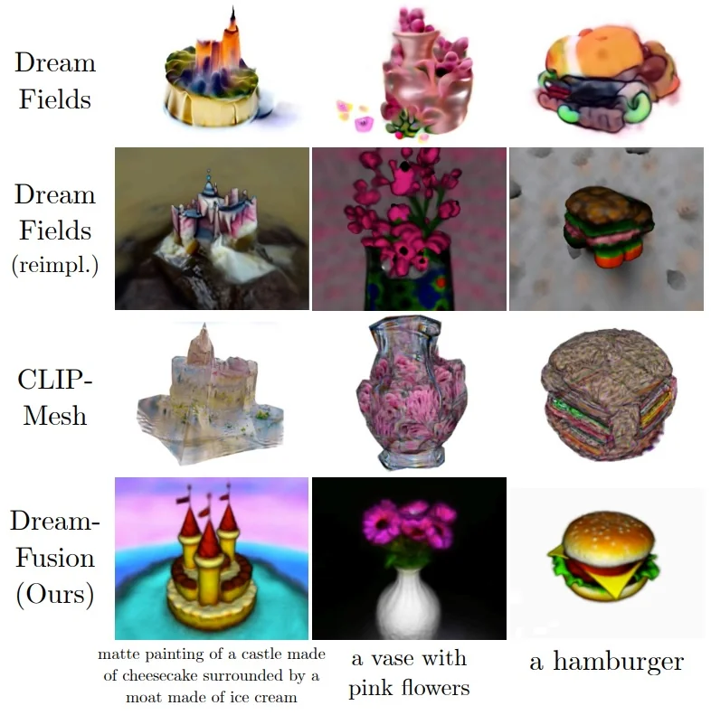
Caption–image coherence via CLIP retrieval Goal. To test whether generated 3D assets truly match their captions, DreamFusion evaluates caption–image coherence using CLIP retrieval, following the protocol in [501]. CLIP serves as a frozen “judge” that compares rendered images against text captions.
Metric (R-Precision). The evaluation is framed as a retrieval task:
R-Precision is the fraction of correct matches. Higher values indicate stronger text–image alignment.
Encoders. Results are reported across three CLIP backbones: B/32, B/16, and L/14. This ensures robustness across different embedding granularities.
Two evaluation modes. To disentangle appearance from geometry, renders are produced under two conditions:
Caveat. Baselines like Dream Fields and CLIP-Mesh are trained directly with CLIP supervision. Their scores may be optimistic when evaluated with the same CLIP family, while DreamFusion relies on a diffusion prior (Imagen) and therefore does not benefit from this alignment.
Findings.
In summary, CLIP retrieval confirms that DreamFusion succeeds not just at painting caption-faithful textures but also at learning consistent 3D geometry that aligns with the text prompt.
Ablations: what unlocks geometry? What we test. Starting from a minimal setup, components are added one at a time to see which choices turn 2D supervision into reliable 3D shape:
Why they matter.
Empirical takeaway. In the ablation (see the below figure), improvements are smallest on albedo evaluations and largest on shaded/textureless evaluations—precisely where geometry matters. The progression
monotonically increases geometry-sensitive R-Precision and visually turns multi-faced, flat subjects into smooth, volumetric shapes with cleaner silhouettes.
Iterative refinement and compositional editing Editing protocol. DreamFusion allows continued optimization from intermediate checkpoints. A single NeRF is retained while the caption is modified, and SDS fine-tuning resumes on the updated text. This means new content is composed onto the existing asset rather than starting over.
What this enables.
Limitations and Future Work
While DreamFusion establishes a powerful pipeline for text-to-3D generation, several limitations remain:
These limitations motivated subsequent methods that trade DreamFusion’s image-space guidance for more efficient latent-space guidance. Approaches such as LatentNeRF [440], Fantasia3D [86], and Magic3D [361] directly distill supervision from latent diffusion models (e.g., Stable Diffusion) rather than pixel-space denoisers. This substantially reduces computational cost while preserving geometric consistency. In addition, Fantasia3D explores disentangled control over geometry and appearance, addressing the shading/material realism issue, while Magic3D introduces a coarse-to-fine optimization pipeline that improves both detail and efficiency.
Looking forward, promising directions include:
In the next part, we examine LatentNeRF, a direct response to DreamFusion’s computational bottlenecks, which achieves faster optimization by shifting SDS guidance from image-space to latent-space, while also keeping/improving the resultant image quality.
Enrichment 23.14.2: Latent-NeRF for Shape-Guided 3D Generation
Motivation
From DreamFusion to Latent-NeRF DreamFusion Enrichment 23.13.2 established that a powerful 2D text-to-image diffusion model can supervise a 3D NeRF via Score Distillation Sampling (SDS), but it operates in RGB space and originally relied on a heavy, proprietary backbone (Imagen). Latent-NeRF adopts the same SDS principle yet relocates supervision and rendering into Stable Diffusion’s VAE latent space \(Z\), thereby reducing computational load while maintaining multi-view consistency through NeRF’s volumetric rendering. Beyond efficiency, the central goal is controllability: text-only guidance is underconstrained in 3D, so the paper introduces Sketch-Shape geometry guidance and Latent-Paint for texturing explicit meshes.
Why latent supervision Volumetric rendering is fundamentally a linear operation that blends feature vectors along rays. The convolutional encoder used in the VAE ensures that each latent vector at coordinate \((u,v)\) encodes a localized patch of pixels, often called a super-pixel. These super-pixels preserve spatial coherence, so interpolating them along a ray produces meaningful blends in latent space. Empirically, decoding linear combinations of latents results in plausible local textures and structures, just as decoding linearly blended RGB colors yields plausible photometric mixtures. This property justifies treating \(\mathbf {Z}\) (typically \(64{\times }64{\times }4\)) as a continuous radiance field suitable for NeRF-style volume rendering, even though its channels are abstract features rather than raw RGB.
In effect, the latent radiance field serves as a dense 3D representation in which NeRF’s differentiable rendering can be applied directly, producing latent images that are natively compatible with Stable Diffusion’s denoiser. This eliminates the bottleneck of pixel-to-latent encoding at each iteration and allows gradients from the diffusion model to flow efficiently into the NeRF.
Method
Overview and connection to DreamFusion Latent-NeRF builds directly on the Score Distillation Sampling (SDS) framework introduced in DreamFusion, but shifts the entire process into the latent space. Whereas DreamFusion renders RGB images from NeRF and then re-encodes them into latents for diffusion guidance, Latent-NeRF trains a NeRF whose outputs are already latents. This simple yet powerful modification removes redundant encoding steps and ensures consistency between the NeRF’s output domain and the Stable Diffusion denoiser.
Concretely, the NeRF MLP maps a 5D input—3D position plus 2D viewing direction—to a volume density \(\sigma \) and a 4-dimensional latent feature vector \(\mathbf {c}\in \mathbb {R}^4\). Standard volumetric rendering integrates these outputs along each ray, yielding a latent image \[ \mathbf {z} \in \mathbb {R}^{64\times 64\times 4}. \]
At each training step, Latent-NeRF applies SDS in latent space:
This procedure is structurally analogous to DreamFusion, but by performing all operations in the latent domain, Latent-NeRF achieves both efficiency and training stability. Subsequent refinement stages can optionally decode the latent radiance field back into RGB using the VAE decoder, enabling high-fidelity visualization while retaining the computational benefits of latent-space supervision.
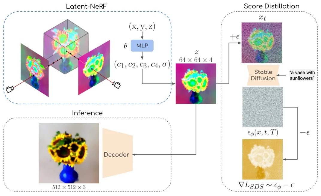
NeRF in Stable Diffusion latent space Given a point \(\mathbf {x}\) and view direction, the MLP outputs \((c_1,c_2,c_3,c_4)\) and density \(\sigma \). Standard volumetric rendering aggregates these along the ray to yield \(\mathbf {z}\). This retains the multi-view coupling of NeRF while aligning supervision to the latent domain where the teacher denoiser operates.
SDS in latent space At each step, with \(\varepsilon \!\sim \!\mathcal {N}(0,I)\) and schedule constant \(\bar \alpha _t\), \begin {equation} x_t \;=\; \sqrt {\bar \alpha _t}\,x \;+\; \sqrt {1-\bar \alpha _t}\,\varepsilon , \end {equation} and the per-pixel SDS gradient is \begin {equation} \nabla _x \mathcal {L}_{\mathrm {SDS}} \;=\; w(t)\,\big (\,\varepsilon _\phi (x_t,t,T)\;-\;\varepsilon \,\big ), \end {equation} where \(\varepsilon _\phi \) denotes the denoiser, \(T\) is the prompt, and \(w(t)\) depends on the noise schedule. Latent-NeRF minimizes \begin {equation} \mathcal {L} \;=\; \lambda _{\mathrm {SDS}}\,\mathcal {L}_{\mathrm {SDS}} \;+\; \lambda _{\mathrm {sparse}}\,\mathcal {L}_{\mathrm {sparse}}, \label {eq:chapter23_latentnerf_textonly_loss} \end {equation} with \(\mathcal {L}_{\mathrm {sparse}}=\mathrm {BE}(w_{\mbox{blend}})\) to suppress floaters/background fog.
# Pretrained Stable Diffusion: encoder E, decoder D, UNet eps_phi
# Radiance field f_theta: (x, y, z, d) -> (c1..c4, sigma)

for step in range(num_steps):
    # 1) Random camera pose; render latent z via volumetric rendering
    z = render_latent(f_theta, sample_camera())

    # 2) Pick diffusion time t and add noise
    t = sample_t()
    eps = torch.randn_like(z)
    x_t = sqrt(alpha_bar[t]) * z + sqrt(1 - alpha_bar[t]) * eps

    # 3) Denoise with text T and form SDS gradient wrt z
    eps_pred = eps_phi(x_t, t, T)                # Stable Diffusion UNet
    g_sds = w(t) * (eps_pred - eps)

    # 4) Backprop through rendering to update theta
    loss_main = (g_sds.detach() * z).sum()     # autograd handles chain rule
    loss_sparse = binary_entropy(w_blend(z))
    loss = lambda_sds*loss_main + lambda_sparse*loss_sparse
    loss.backward()
    optimizer.step()
    optimizer.zero_grad()
Rendering and latent image formation Let \(\{\mathbf {x}_i\}_{i=1}^{N}\) be the stratified samples along a camera ray with spacings \(\Delta _i\). The field outputs \((\mathbf {c}_i,\sigma _i)=f_\theta (\mathbf {x}_i,\mathbf {d})\) where \(\mathbf {c}_i\in \mathbb {R}^4\) are Stable-Diffusion VAE latents and \(\sigma _i\ge 0\) are densities. Using standard alpha compositing: \begin {align} \alpha _i &= 1 - \exp (-\sigma _i \Delta _i), \qquad T_i \;=\;\prod _{j<i} (1-\alpha _j), \label {eq:chapter23_latentnerf_alphaTi}\\ w_i &= T_i \,\alpha _i, \qquad \mathbf {z}(u,v) \;=\; \sum _{i=1}^{N} w_i \,\mathbf {c}_i \;\in \; \mathbb {R}^{4}, \label {eq:chapter23_latentnerf_z} \end {align}
so the rendered latent image \(\mathbf {z}\in \mathbb {R}^{64\times 64\times 4}\) is obtained by evaluating ([ref]) per pixel \((u,v)\).
Diffusion guidance in latent space (SDS) For a randomly drawn diffusion step \(t\) and Gaussian noise \(\varepsilon \!\sim \!\mathcal {N}(0,I)\), the forward noising is \begin {equation} x_t \;=\; \sqrt {\bar \alpha _t}\,\mathbf {z} \;+\; \sqrt {1-\bar \alpha _t}\,\varepsilon , \label {eq:chapter23_latentnerf_eq1} \end {equation} and the per-pixel SDS gradient applied to \(\mathbf {z}\) is \begin {equation} \nabla _{\mathbf {z}} \mathcal {L}_{\mathrm {SDS}} \;=\; w(t)\,\big (\,\varepsilon _\phi (x_t,t,T)\;-\;\varepsilon \,\big ), \label {eq:chapter23_latentnerf_eq2} \end {equation} where \(\varepsilon _\phi \) is the frozen Stable Diffusion denoiser and \(w(t)\) follows the noise schedule (scaling can absorb the \(\sqrt {1-\bar \alpha _t}\) factor used in some SDS variants). Gradients backpropagate through (§20) and (§20) into \(\theta \).
Classifier-free guidance (CFG) in latent SDS When using CFG, the denoiser is queried twice (with/without the text): \begin {equation} \hat \varepsilon _{\mathrm {cfg}} \;=\; (1+s)\,\varepsilon _\phi (x_t,t,T)\;-\;s\,\varepsilon _\phi (x_t,t,\varnothing ), \quad s\ge 0, \label {eq:chapter23_latentnerf_cfg} \end {equation} and \(\varepsilon _\phi \) in (23.67) is replaced by \(\hat \varepsilon _{\mathrm {cfg}}\). This preserves the SDS form while strengthening text adherence.
Sparsity / anti-fog regularization A well-known failure mode in NeRF optimization is the tendency to produce “floaters” (detached blobs of density) or a diffuse “fog” spread throughout the volume. Both artifacts can satisfy the supervision signal (e.g., SDS) from certain views, but they yield incoherent or implausible 3D structure. To combat this, Latent-NeRF introduces a sparsity prior on the ray termination probability.
Let \(w_i\) denote the volumetric weight at sample \(i\) along a ray, and define the ray’s termination probability as \[ w_{\mathrm {term}} \;=\; \sum _i w_i \;=\; 1 - T_{N+1}, \] where \(T_{N+1}\) is the residual transmittance at the end of the ray. Intuitively, \(w_{\mathrm {term}}\) measures whether the ray “hit something” (value close to 1) or passed entirely through empty space (value close to 0).
The sparsity penalty applies the binary entropy function: \begin {equation} \mathcal {L}_{\mathrm {sparse}} \;=\; -\;w_{\mathrm {term}}\log w_{\mathrm {term}} -\;(1-w_{\mathrm {term}})\log (1-w_{\mathrm {term}}). \label {eq:chapter23_latentnerf_sparse} \end {equation}
Why this works.
Effect on geometry. Minimizing \(\mathcal {L}_{\mathrm {sparse}}\) discourages semi-transparent mass and pushes density into compact, surface-like structures. This leads to:
Relation to other regularizers. This objective serves the same purpose as the “opacity penalty” in DreamFusion and resembles distortion-based losses in Mip-NeRF 360, which also discourage opacity from being spread diffusely along rays. The key distinction here is its simplicity: the binary entropy prior directly penalizes uncertainty in ray termination, providing a lightweight yet effective “anti-fog” constraint that integrates seamlessly with SDS.
Total objective (normal/text-only mode) Combining latent SDS with sparsity yields: \begin {equation} \mathcal {L}_{\mbox{total}} \;=\; \lambda _{\mathrm {SDS}}\;\mathcal {L}_{\mathrm {SDS}} \;+\; \lambda _{\mathrm {sparse}}\;\mathcal {L}_{\mathrm {sparse}}, \label {eq:chapter23_latentnerf_total_objective} \end {equation} with \(\mathcal {L}_{\mathrm {SDS}}\) applied by integrating (23.67) over all pixels of \(\mathbf {z}\) for the current camera. Typical implementation details include:
Sketch-Shape guidance: Rationale and Mechanism Why it is needed. Text-to-3D generation guided only by natural language is often underspecified: prompts such as “a wooden chair” or “a German Shepherd” describe appearance but rarely pin down a unique geometry. This lack of geometric priors can produce ambiguous or unstable reconstructions (e.g., Janus-like multiple faces, inconsistent body proportions). To mitigate this, Latent-NeRF introduces Sketch-Shape guidance, which supplies a coarse 3D proxy (e.g., composed of primitive shapes or a rough mesh) that defines global structure and pose. The text prompt then refines this scaffold by providing details, texture, and style. This decoupling of geometry (from the Sketch-Shape) and appearance (from text guidance) yields controllable, stable synthesis.
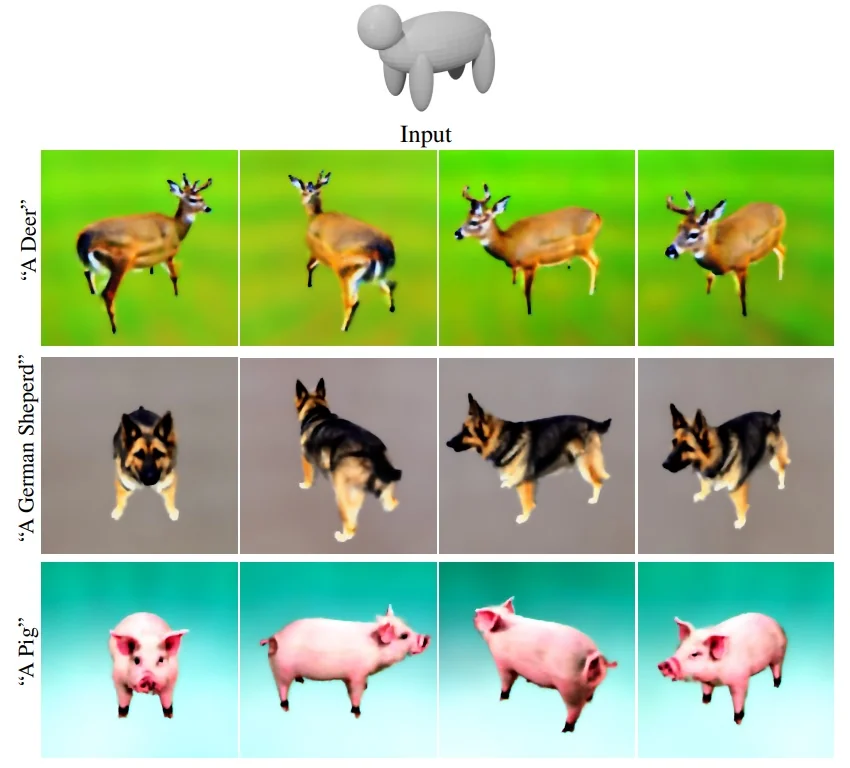
How it works. The coarse shape is converted into a binary occupancy function, \(\alpha _{\mbox{GT}}(p)\in \{0,1\}\), which marks whether a sampled point \(p\) along a camera ray lies inside or outside the proxy. The NeRF MLP is not replaced by a separate network; rather, the same radiance field MLP outputs its usual density \(\sigma \) and opacity \(\alpha _{\mbox{NeRF}}(p)\). A distance-weighted cross-entropy loss then encourages \(\alpha _{\mbox{NeRF}}\) to match \(\alpha _{\mbox{GT}}\):
\begin {equation} \mathcal {L}_{\mbox{Sketch-Shape}} \;=\; \mathrm {CE}\!\big (\alpha _{\mbox{NeRF}}(p),\,\alpha _{\mbox{GT}}(p)\big )\cdot \!\Big (1 - e^{-\tfrac {d^2}{2\sigma _S^2}}\Big ), \label {eq:chapter23_latentnerf_eq4} \end {equation}
where \(d\) is the distance from \(p\) to the Sketch-Shape surface, and \(\sigma _S\) controls the softness of the constraint.
Interpretation of the weighting. The exponential term modulates how strictly the constraint is enforced:
The parameter \(\sigma _S\) tunes this tradeoff: small values enforce tight adherence to the proxy, while larger values allow more stylistic freedom.
Integration. The Sketch-Shape loss is evaluated on the same set of ray samples already used for volumetric rendering, so no additional forward passes are needed. The NeRF MLP remains the sole predictor of densities and latents; the proxy only contributes distance and occupancy values for loss computation. This design makes Sketch-Shape guidance a lightweight addition that integrates seamlessly with the main SDS optimization, combining coarse geometric supervision with text-driven refinement.
Effect of the leniency parameter \(\sigma _S\) Increasing \(\sigma _S\) relaxes the constraint, enabling the NeRF geometry to deviate more from the input shape under textual pressure.
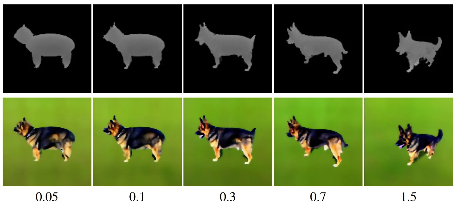
Latent-Paint for explicit meshes When an explicit mesh with known UV coordinates is available, Latent-Paint enables texture optimization directly in the Stable Diffusion latent space.
UV coordinates. UVs are a standard graphics convention for mapping points on a 3D surface to positions in a 2D texture image. Each vertex on the mesh is assigned a \((u,v)\) coordinate in \([0,1]^2\), so that a 2D image can be “wrapped” around the 3D surface. If a mesh does not come with UVs, they can be automatically computed with algorithms such as XAtlas, which unfold the surface into a set of non-overlapping charts.
Mechanism. Latent-Paint defines a latent texture image \(\Theta \in \mathbb {R}^{H\times W\times 4}\) in the same 4-channel space as Stable Diffusion’s VAE. Differentiable rasterization maps each triangle of the mesh to the corresponding latent pixels of \(\Theta \), producing a rendered latent image from a given camera viewpoint. This image is then supervised by the same latent SDS rule used in Latent-NeRF: it is noised, denoised by the Stable Diffusion UNet, and the residual between predicted and injected noise provides gradients. These gradients backpropagate through the differentiable renderer to update the pixels of \(\Theta \).
After convergence, a single decode of \(\Theta \) with the VAE decoder produces a high-resolution RGB texture image. The benefit of this approach is that it avoids per-pixel optimization in RGB space and instead leverages Stable Diffusion’s compact latent representation to guide texture generation efficiently.
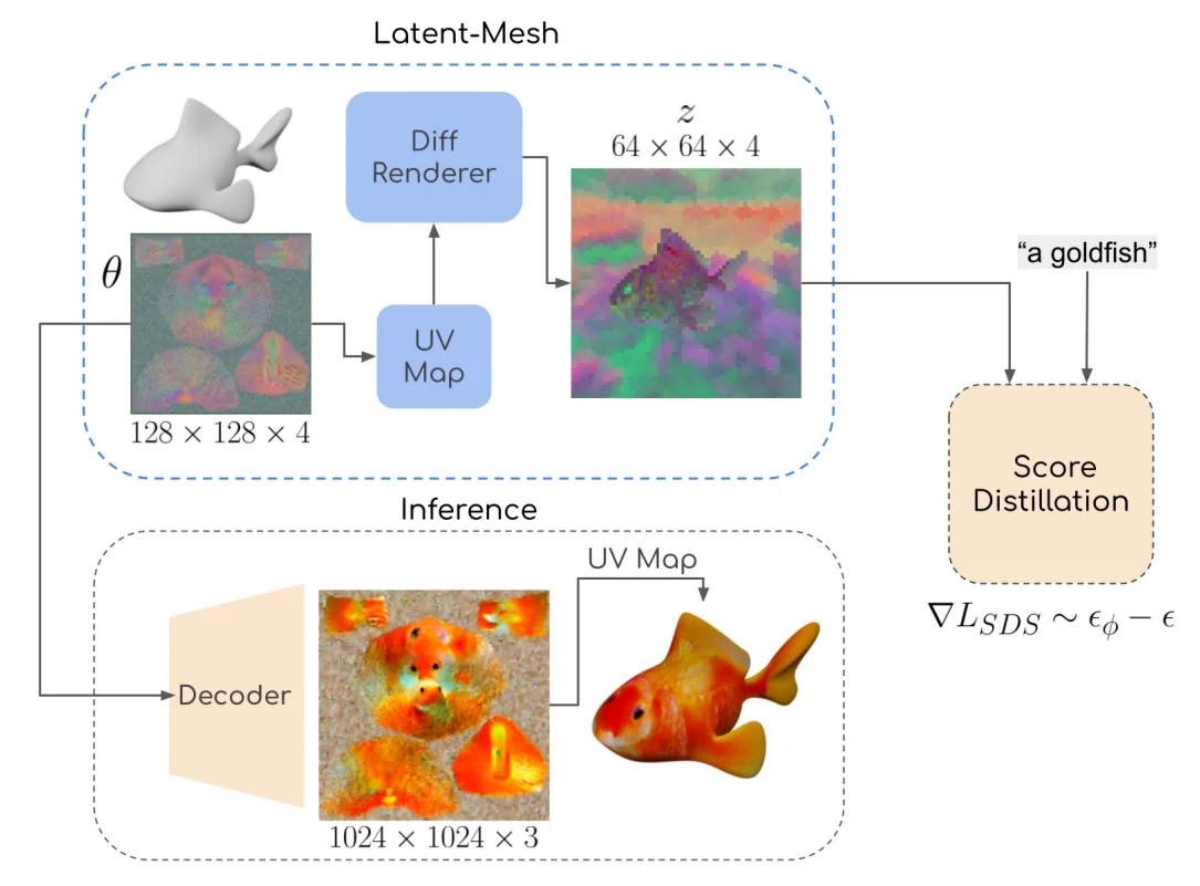
RGB refinement with a learnable linear adapter Although latent-space training is efficient, many applications (visualization, export, rendering) require a NeRF that emits RGB directly. To bridge this gap, Latent-NeRF adds a small linear adapter on top of the NeRF’s four latent output channels \((c_1,\ldots ,c_4)\). This adapter maps the latent channels to approximate RGB \((\hat r,\hat g,\hat b)\) using a \(3{\times }4\) matrix, initialized to a hand-fit linearization of the Stable Diffusion VAE decoder: \begin {equation} \begin {pmatrix}\hat r\\[2pt]\hat g\\[2pt]\hat b\end {pmatrix} = \begin {pmatrix} 0.298 & 0.187 & -0.158 & -0.184\\ 0.207 & 0.286 & \phantom {-}0.189 & -0.271\\ 0.208 & 0.173 & \phantom {-}0.264 & -0.473 \end {pmatrix} \begin {pmatrix}c_1\\[2pt]c_2\\[2pt]c_3\\[2pt]c_4\end {pmatrix}. \label {eq:chapter23_latentnerf_eq3} \end {equation} This initialization is only a starting point; the matrix is made trainable and updated during refinement.
What parameters are trained.
Both components co-adapt: the NeRF learns to emit latent features that decode to better colors, and the adapter learns how to colorize those features effectively.
How RGB participates in the loss.
Thus, even though the supervision remains in \(Z\), the RGB pathway matters: the only way to make \(z'\) align with the text-conditioned score is to render RGB that, when re-encoded, produces better latents. This couples pixel-space fidelity to the latent-space objective.
Why this matrix and how it improves.
Why refinement helps.
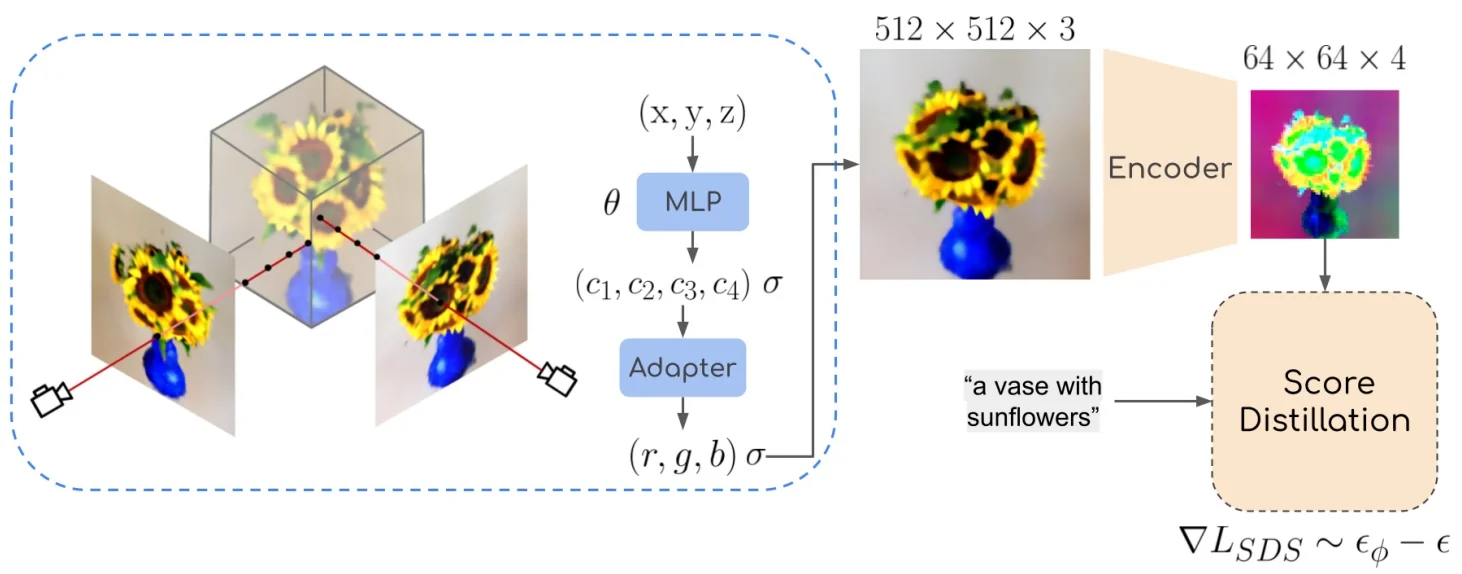
Architecture and Implementation Details
Backbones Stable Diffusion v1-4 (HuggingFace Diffusers) provides the VAE \((E,D)\) and UNet denoiser \(\varepsilon _\phi \); Instant-NGP serves as the NeRF backbone for efficiency. Latent rendering uses \(64{\times }64{\times }4\) maps; Latent-Paint uses \(H\!=\!W\!=\!128\) latent textures by default.
Schedules and regularizers SDS uses Eq. 23.66–23.67 with \(w(t)\) tied to the diffusion schedule. A binary-entropy sparsity term \(\mathrm {BE}(w_{\mbox{blend}})\) suppresses floaters and encourages strict object/background blending. Sketch-Shape uses Eq. 23.71 over the point set already sampled for volumetric rendering.
Experiments and Ablations
Text-only generation and multi-view consistency Latent-NeRF produces coherent 3D assets under text-only guidance; view sweeps confirm stable geometry and appearance.
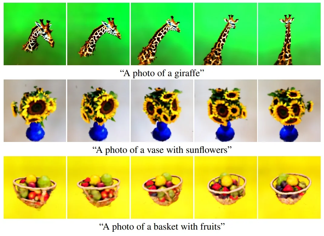
Qualitative comparison Against DreamFields, CLIPMesh, and DreamFusion, Latent-NeRF typically shows sharper textures and more plausible geometry for identical prompts.
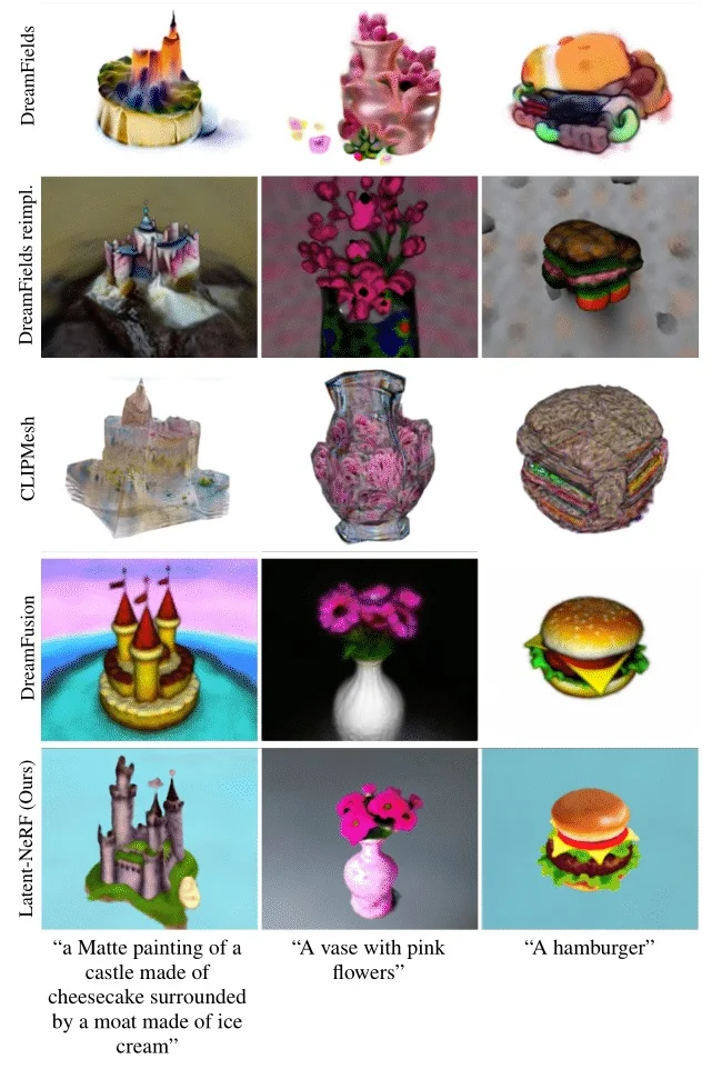
RGB refinement improvements Refinement enhances high-frequency detail (textures, material cues) beyond what the VAE decoder alone produces.
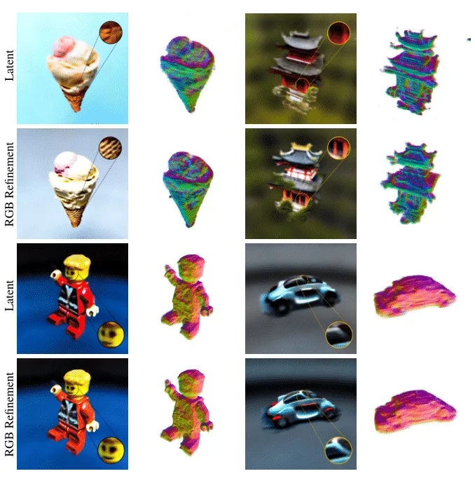
Controllability via Sketch-Shape Using identical prompts with and without shape guidance reveals strong benefits for geometric coherence.
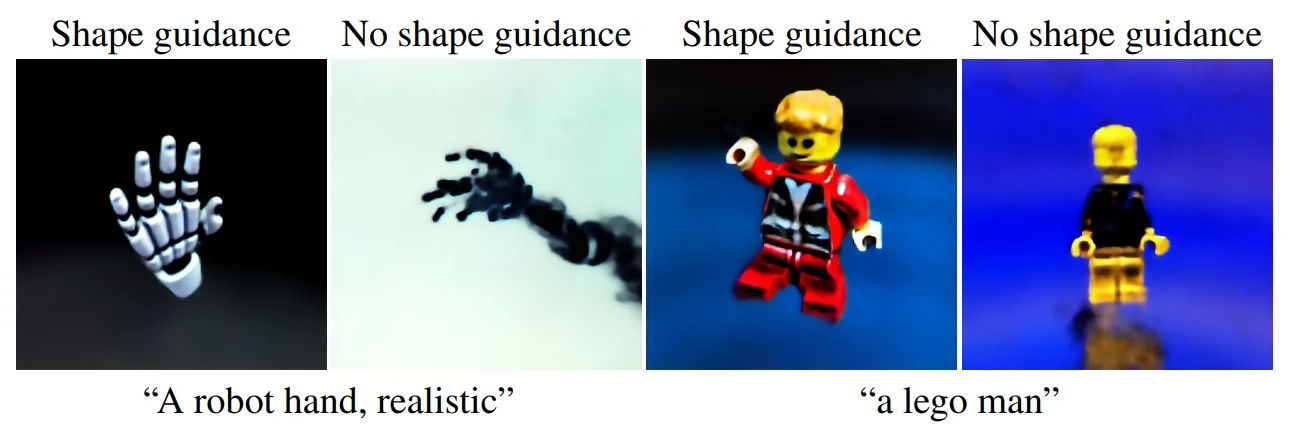
More Sketch-Shape results A simple house prior can be styled in multiple ways; further examples span hands, toys, and vehicles.
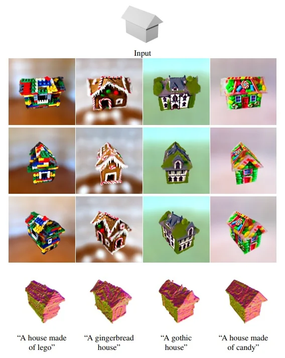
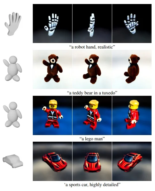
Latent-Paint on generic meshes Text-driven textures can be applied to shapes without UVs (computed on-the-fly) or with precomputed UVs.
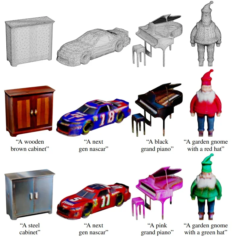
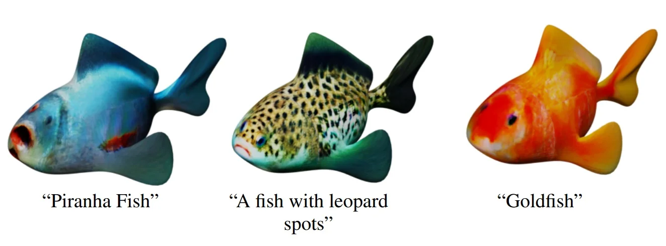
Texturing comparison on a common mesh Latent-Paint produces textures that are more realistic and prompt-faithful than CLIP-guided baselines.
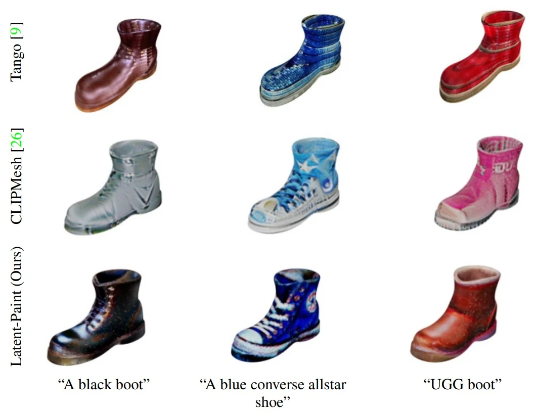
Personalization via Textual Inversion Latent-NeRF inherits the ability to use learned tokens for novel objects/styles, enabling faithful reconstruction and creative composition.
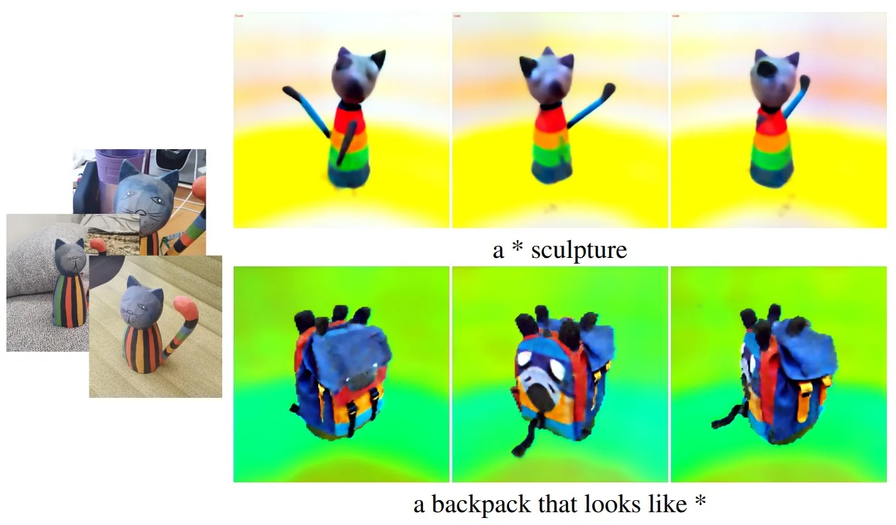
Limitations and Future Work
View ambiguity and Janus artifacts Because Latent-NeRF relies on a 2D prior, supervision for unseen views is weak. This often causes Janus artifacts, such as multi-faced geometry (e.g., a squirrel with two faces), where the denoiser defaults to canonical front views rather than plausible backs.
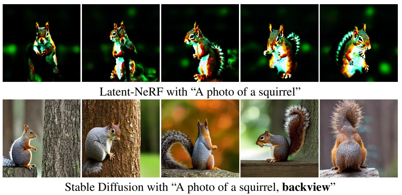
Controllability and future directions Controllability remains limited: results vary with seed, and prompts can be ambiguous. The paper mitigates this with shape priors (Sketch-Shape), explicit texturing (Latent-Paint), and opacity regularization, but these do not fully solve view inconsistency. Future directions include integrating other, possibly stronger, 3D priors (depth or normal cues), exploring 3D-native diffusion backbones, and extending beyond UV textures to richer material models such as BRDFs.