Lecture 6: Backpropagation

6.1 Introduction: The Challenge of Computing Gradients

In the previous lecture, we explored how neural networks exploit non-linear space warping to form complex decision boundaries—far surpassing the capabilities of linear classifiers. While activation functions like ReLU make this possible, they introduce a key question:

How do we efficiently compute gradients for neural networks with millions or billions of parameters?

Traditional numerical or purely symbolic differentiation methods quickly become:

• Scalability Bottlenecks: Deriving gradients manually does not scale to deep networks.
• High Computational Complexity: Efficient gradient computation is non-trivial at large scales.
• Limited Modularity: Any architectural modification (e.g., adding layers, changing the loss) requires recalculating derivatives from scratch.

6.1.1 A Bad Idea: Manually Deriving Gradients

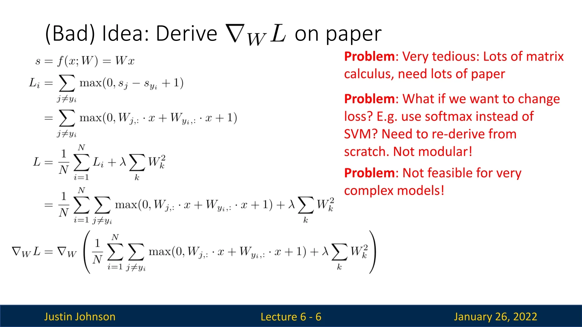
One naive approach is to derive all gradients by hand. As shown in Figure 6.1, it might be doable for basic linear models. Nevertheless, it also clearly demonstrates some of the problems described in the introduction (very tedious and error-prone), and mostly, it gives us a hint to how complex this process will be for more complex models like neural networks, with many layers and millions up to billions of parameters. Hence, this approach is impractical, and we need to think of a better idea to compute gradients for the neural network optimization task.

6.1.2 A Better Idea: Utilizing Computational Graphs (Backpropagation)

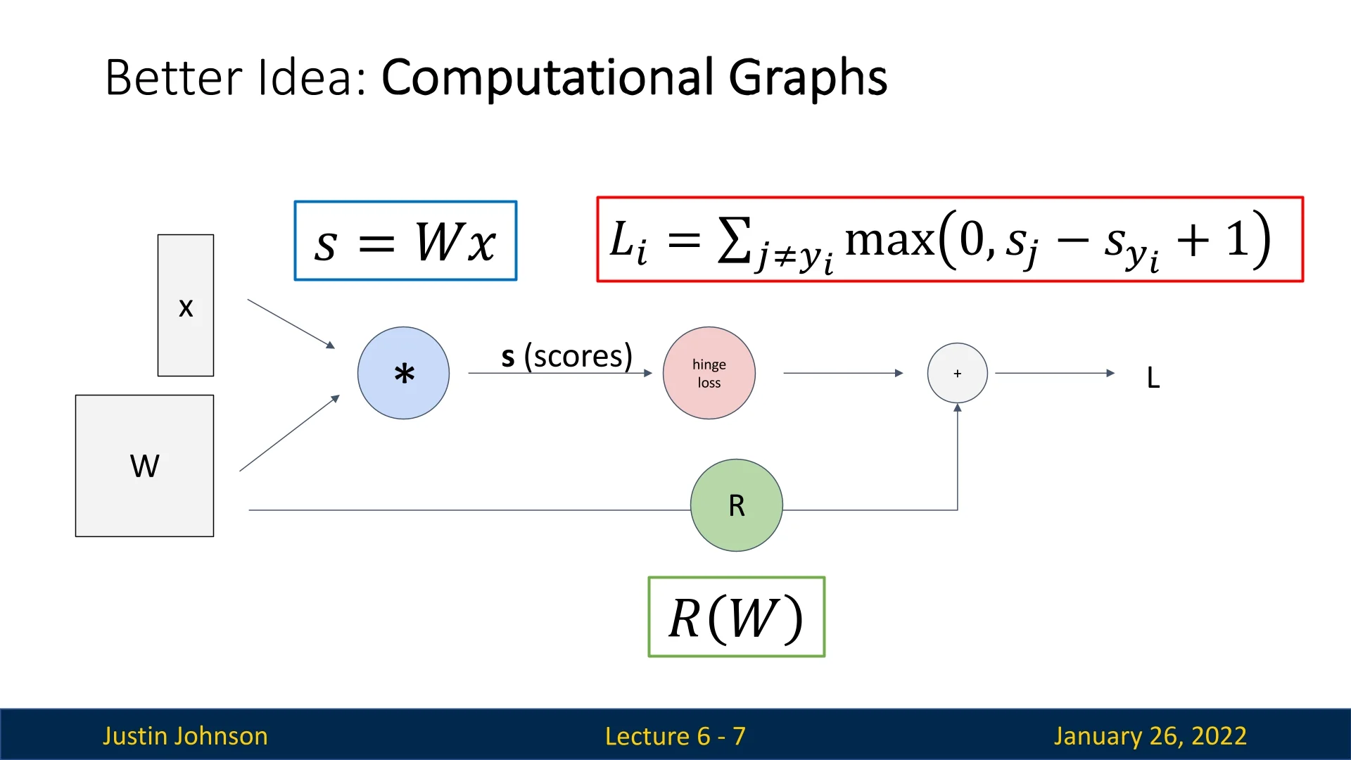
A more robust solution is to represent computations as a computational graph:

• Each node in the graph performs a specific operation (e.g., addition, matrix multiplication, or more complex operations like ReLU based on more basic primitives).
• Edges represent the flow of intermediate values (outputs of one operation become inputs to the next).
• Backpropagation can be used to automatically compute the gradient at each node by systematically applying the chain rule in reverse. Hence, each node in the graph only does simple local computations (derives the downstream gradients using a multiplication of the local gradient and the upstream gradient received from a following node). We’ll see several examples of backpropagation later to understand what do we mean by that and what makes it important.

Why Use Computational Graphs?

• Modularity: Swap loss functions, activation layers, or architectures without manually re-deriving gradients.
• Scalability: Supports deep networks with millions of parameters, keeping computations local to each node.
• Automation: Greatly reduces human error and development time.

6.2 Toy Example of Backpropagation: \(f(x,y,z) = (x + y)\,z\)

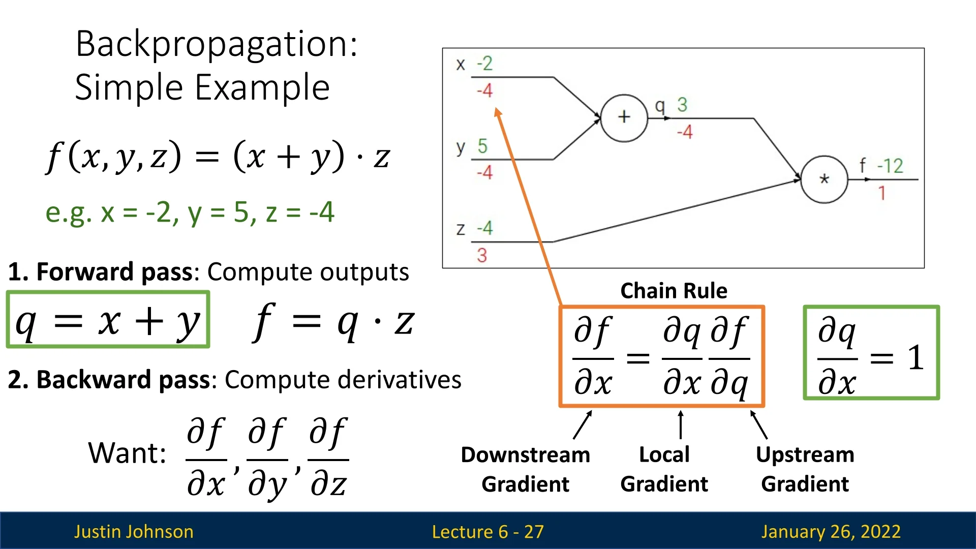
Consider a simple function: \[ f(x,y,z) = (x + y)\,z, \] with \(x = -2\), \(y = 5\), and \(z = -4\).

6.2.1 Forward Pass

We traverse the graph from left to right:

• \(\displaystyle q = x + y = -2 + 5 = 3.\)
• \(\displaystyle f = q \cdot z = 3 \times (-4) = -12.\)

6.2.2 Backward Pass: Computing Gradients

To find \(\frac {\partial f}{\partial x}, \frac {\partial f}{\partial y}, \frac {\partial f}{\partial z}\), we apply the chain rule:

• \(\displaystyle \frac {\partial f}{\partial z} = q = 3.\)
• \(\displaystyle \frac {\partial f}{\partial q} = z = -4.\)
• \(\displaystyle \frac {\partial f}{\partial y} = \frac {\partial f}{\partial q} \times \frac {\partial q}{\partial y} = (-4) \times 1 = -4.\)
• \(\displaystyle \frac {\partial f}{\partial x} = \frac {\partial f}{\partial q} \times \frac {\partial q}{\partial x} = (-4) \times 1 = -4.\)

6.3 Why Backpropagation?

6.3.1 Local & Scalable Gradients Computation

As we’ve seen in the above examples, within the computational graph, each node performs only local gradient calculations. This is the core principal behind backpropagation, making it scalable and practical. Therefore, in order to make sure we clearly understand why, we’ll zoom out and provide a high-level overview looking only at an abstract node in a computational graph independently.

Suppose a node \(f\) outputs \(z\) from inputs \(x\) and \(y\). Given an upstream gradient \(\frac {\partial L}{\partial z}\) (the partial derivative of the loss \(L\) w.r.t. \(z\)), the node only needs:

• \(\displaystyle \frac {\partial z}{\partial x}\),
• \(\displaystyle \frac {\partial z}{\partial y}\),

to compute: \[ \frac {\partial L}{\partial x} \;=\; \frac {\partial z}{\partial x} \;\times \; \frac {\partial L}{\partial z}, \quad \frac {\partial L}{\partial y} \;=\; \frac {\partial z}{\partial y} \;\times \; \frac {\partial L}{\partial z}. \]

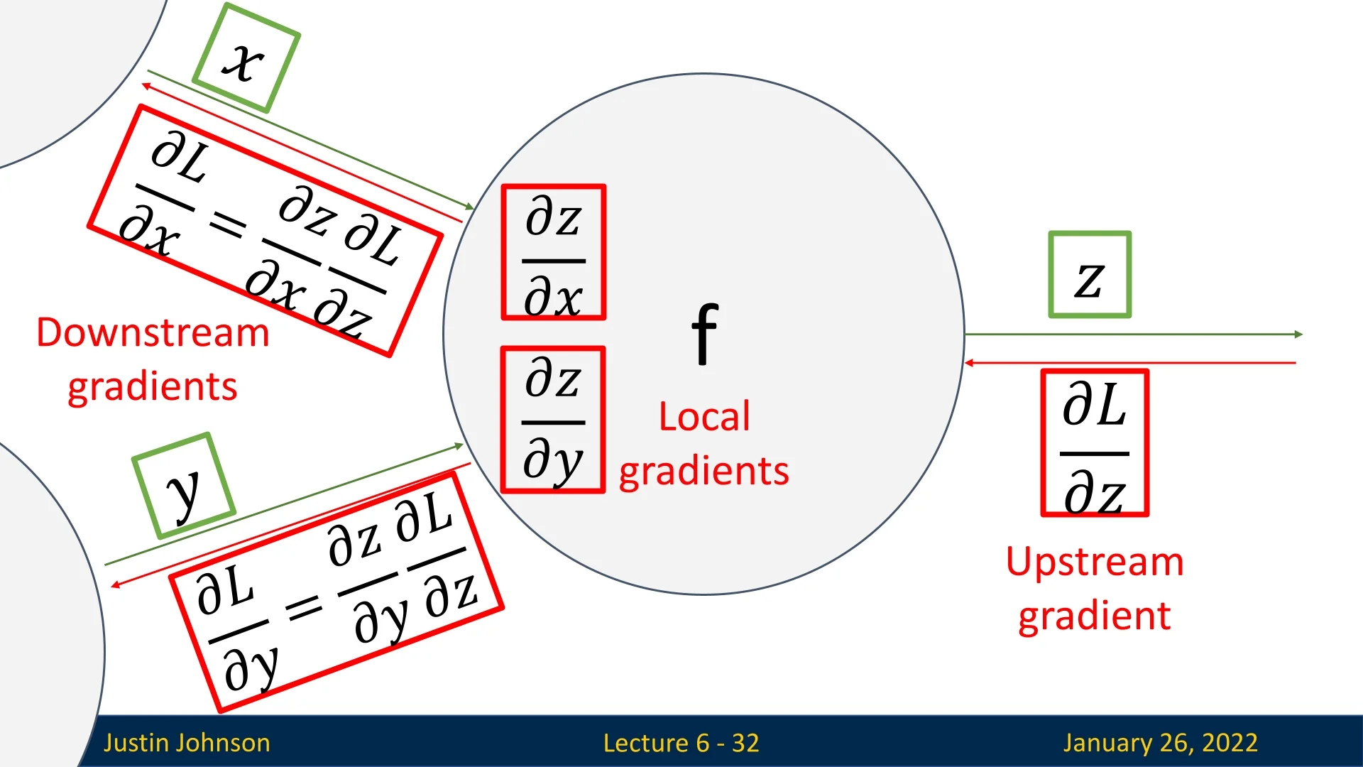
The local multiplication by \(\frac {\partial L}{\partial z}\) (the upstream gradient) ensures each node can be implemented and debugged independently, enabling large-scale networks to remain tractable. This demonstrates the power and essence behind backpropagation for complex models, making it the go-to approach for gradients computation in neural networks optimization.

6.3.2 Pairing Backpropagation Gradients & Optimizers is Easy

While backpropagation efficiently provides the necessary gradients for each parameter, we still need gradient-based optimizers to use those gradients in gradient descent updates. In practice, we pair backprop with methods like Stochastic Gradient Descent (SGD) or AdamW, which adjust parameters based on the gradients to minimize the loss. This synergy—automatic gradient computation via backprop, combined with iterative updates via gradient descent—enables neural networks to learn effectively from large and complex datasets.

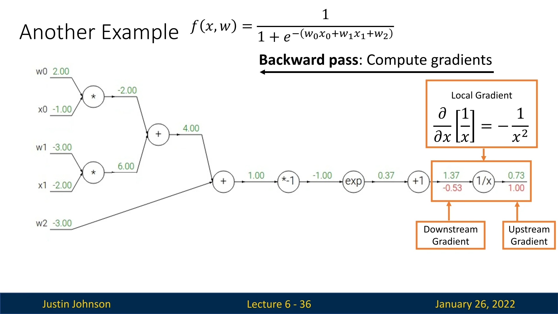
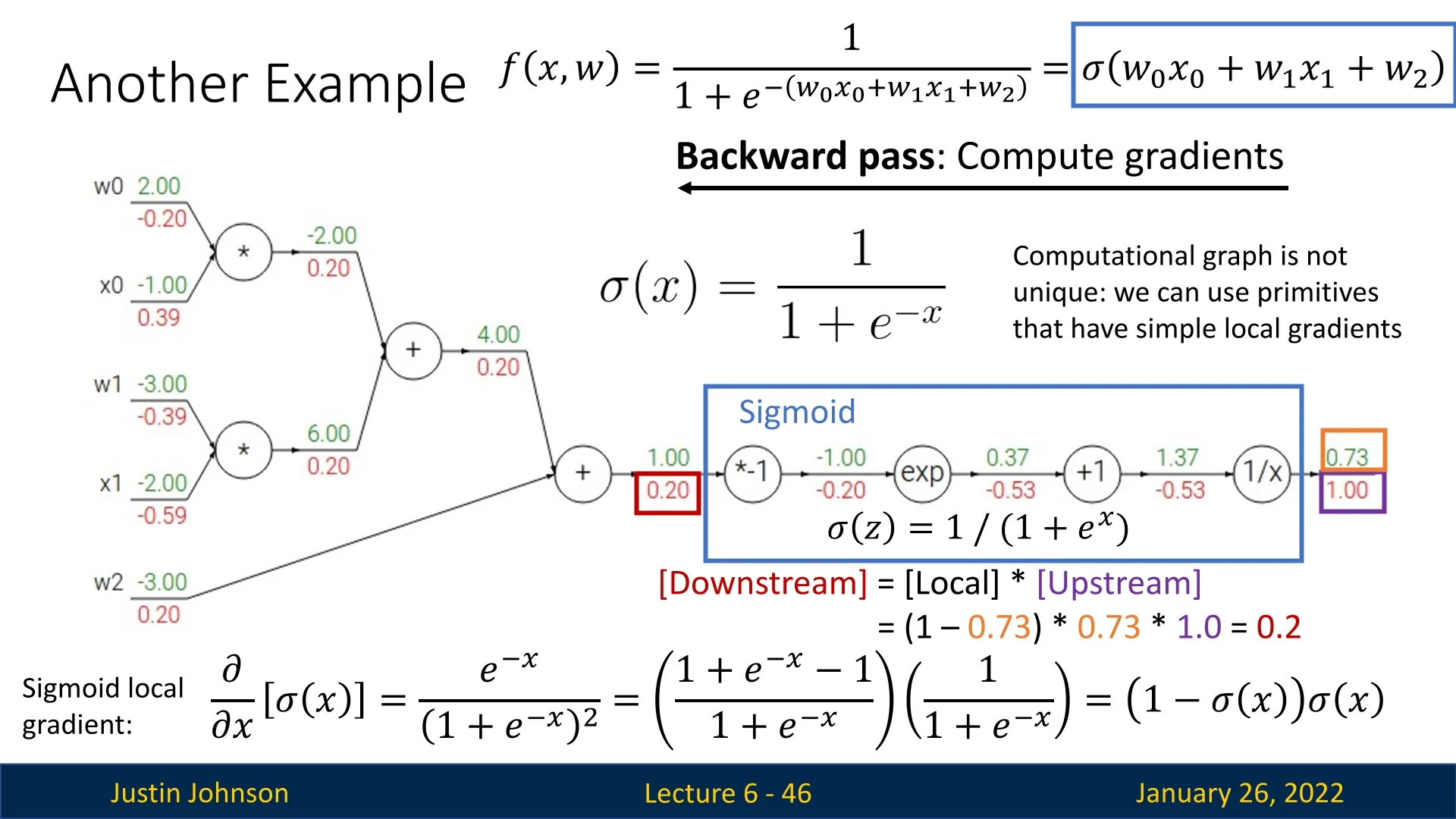
6.3.3 Modularity and Custom Nodes

Because the computation graph decomposes into local operations, we can define specialized nodes for common functions. For example, a “sigmoid node” encapsulates the sigmoid function: \[ \sigma (x) = \frac {1}{1 + e^{-x}}, \] and uses the known derivative \(\sigma '(x) = \sigma (x)\bigl (1 - \sigma (x)\bigr )\) to backpropagate efficiently. This approach:

• Simplifies the computational graph, reducing intermediate steps.
• Improves memory efficiency (fewer nodes, less storage for intermediate values).
• Allows us to treat the sigmoid as a single, optimized building block in our network, making the graph more semantically meaningful.

6.3.4 Utilizing Patterns in Gradient Flow

Backpropagation is not just a mechanical process of computing derivatives; it follows structured gradient flow patterns that help us analyze and design computational graphs more effectively. By understanding these patterns, we can quickly construct computational graphs, debug gradient propagation issues, and optimize network structures.

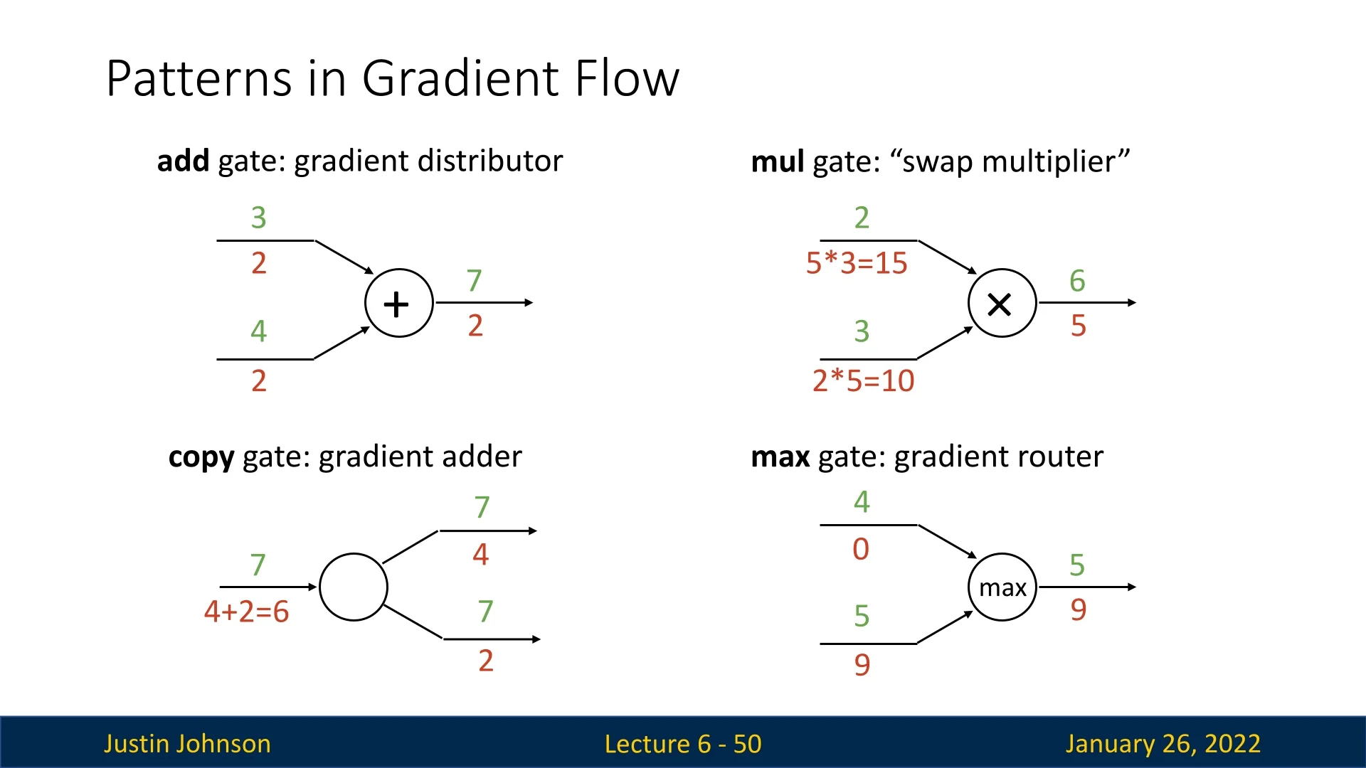
6.3.5 Addition Gate: The Gradient Distributor

The add gate acts as a gradient distributor during the backward pass. When a function locally computes the output as the sum of its inputs, the local gradients for each input are simply 1. Thus, the downstream gradient for each input is equal to the upstream gradient, making it straightforward to propagate gradients backward.

This pattern also provides an intuition about how gradient flow behaves in models that use addition operations, such as residual connections in deep networks which we’ll extensively cover later.

6.3.6 Copy Gate: The Gradient Adder

The copy gate (or copy node) is a trivial operation in the forward pass—it simply duplicates its input. However, it is useful when the same term appears in multiple parts of a computational graph.

For instance, weight matrices are shared across different parts of a loss function:

• In one path, they compute intermediate values such as \( h = Wx + b \).
• In another path, they contribute to the regularization term (e.g., L1/L2 regularization).

Since the weight matrix is reused, the backward pass must account for all gradient contributions. The copy gate accumulates gradients by summing all upstream gradients and passing the combined result as its downstream gradient.

Interestingly, the add and copy gates are dual operations:

• The forward operation of the add gate behaves like the backward operation of the copy gate.
• The forward operation of the copy gate behaves like the backward operation of the add gate.

6.3.7 Multiplication Gate: The Gradient Swapper

The multiplication gate (or mul gate) swaps the roles of its inputs in the backward pass. For the function \[ f(x,y) = x \cdot y, \] the local gradients are \[ \frac {\partial f}{\partial x} = y, \quad \frac {\partial f}{\partial y} = x. \] Hence:

• The downstream gradient for \(y\) is \(x\) times the upstream gradient,
• The downstream gradient for \(x\) is \(y\) times the upstream gradient.

This mixing of gradients can lead to:

• Exploding gradients: Large products magnify updates, destabilizing training,
• Vanishing gradients: Small products reduce gradient magnitudes, slowing convergence.

6.3.8 Max Gate: The Gradient Router

The max gate selects the largest input value in the forward pass and routes the entire upstream gradient to that winning input in the backward pass. All other inputs receive zero gradient. While intuitive, this creates gradient starvation: only one path in the computational graph receives a nonzero gradient, potentially slowing learning.

6.4 Implementing Backpropagation in Code

Now that we understand gradient flow patterns, how can we implement backpropagation in practice? One approach is to compute the flat gradient code. This method directly computes gradients step by step without leveraging modular APIs such as PyTorch’s autograd. While simple, it lacks flexibility.

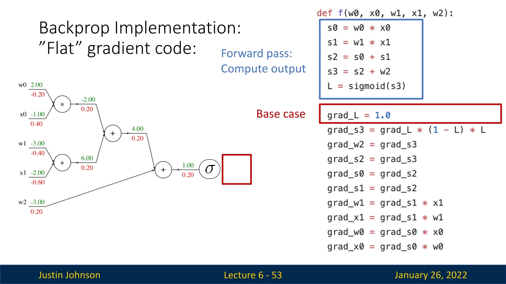
6.4.1 Flat Backpropagation: A Direct Approach

The forward pass follows naturally from the computational graph, while the backward pass appears as a reversed version of it. The process begins with the base case: \[ \texttt{grad_L} = 1.0 \] (i.e., the gradient of the loss with respect to itself is 1), and then we propagate gradients in reverse order.

A step-by-step breakdown:

• The loss is computed after applying a sigmoid activation, so we begin by computing the local gradient of the sigmoid function: \[ \frac {d}{dx} \sigma (x) = \sigma (x) \cdot (1 - \sigma (x)). \] Since \(\sigma (x)\) is the output of the sigmoid function (denoted as \(L\)), we get: \[ \texttt{grad_s3} = \texttt{grad_L} \cdot (1 - L) \cdot L. \]
• The add gate distributes grad_s3 equally to its inputs, propagating gradients further back in the graph.
• The final two mul gates act as swapped multipliers, computing gradients for each input based on the values of the other.

Why Flat Backpropagation Works Well. Despite its simplicity, this approach correctly computes gradients without manually deriving them. However, it has major limitations:

• Non-Modular: Any change in the model or loss function requires rewriting the gradient code from scratch.
• Hard to Scale: Flat implementations do not easily extend to deep architectures with many layers.

6.5 A More Modular Approach: Computational Graphs in Practice

A more structured way to implement backpropagation is to use a computational graph API. Instead of manually coding backward passes, we represent the entire model as a graph structure that:

• Stores nodes corresponding to computations.
• Automatically computes gradients by traversing the graph in reverse order.
• Allows modifications to loss functions and architectures without rewriting gradient code.

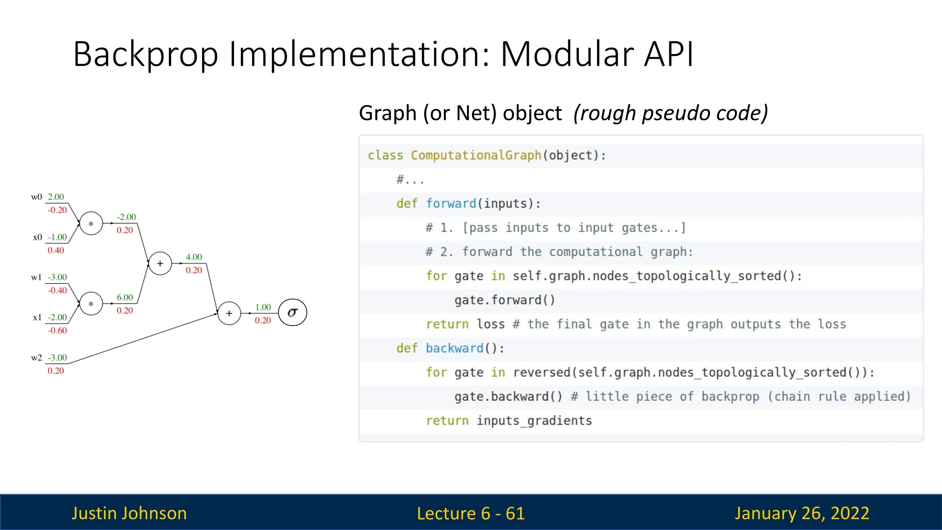
6.5.1 Topological Ordering in Computational Graphs

A computational graph provides an efficient way to manage computations, enabling automatic differentiation and modularity. The graph structure follows a topological ordering, meaning:

• Each node appears before all nodes dependent on it in the forward pass.
• In the backward pass, the nodes are traversed in the reverse order.

This ensures that gradients are properly propagated through the network, following the dependencies established in the forward pass.

6.5.2 The API: Forward and Backward Methods

A computational graph framework defines an API with two essential functions:

1.

forward(): Computes and stores intermediate values for later use in backpropagation.

2.

backward(): Applies the chain rule to compute gradients by traversing the graph in reverse.

Many deep learning frameworks, such as PyTorch, TensorFlow, and JAX, implement automatic differentiation engines based on this principle. These frameworks eliminate the need for manually coding derivatives, making it easier to train deep models.

6.5.3 Advantages of a Modular Computational Graph

Using a computational graph for backpropagation offers several advantages over flat backpropagation:

• Modularity: Changing the model architecture or loss function only requires modifying the forward function, and the backward function is computed automatically.
• Scalability: Works efficiently for deep networks with millions or billions of parameters.
• Automatic Differentiation: Frameworks can compute gradients dynamically, reducing the need for manual derivative calculations.

This modular approach enables modern deep learning frameworks to handle complex architectures efficiently while abstracting away the tedious details of gradient computation.

6.6 Implementing Backpropagation with PyTorch Autograd

A practical example of a modular approach to implementing backpropagation is PyTorch’s Autograd engine. In PyTorch, functions that support automatic differentiation inherit from
torch.autograd.Function. These functions must implement two key static methods:

• Forward: Computes the node’s output and stashes values required for the backward pass.
• Backward: Receives the upstream gradient and propagates it back using local derivatives.

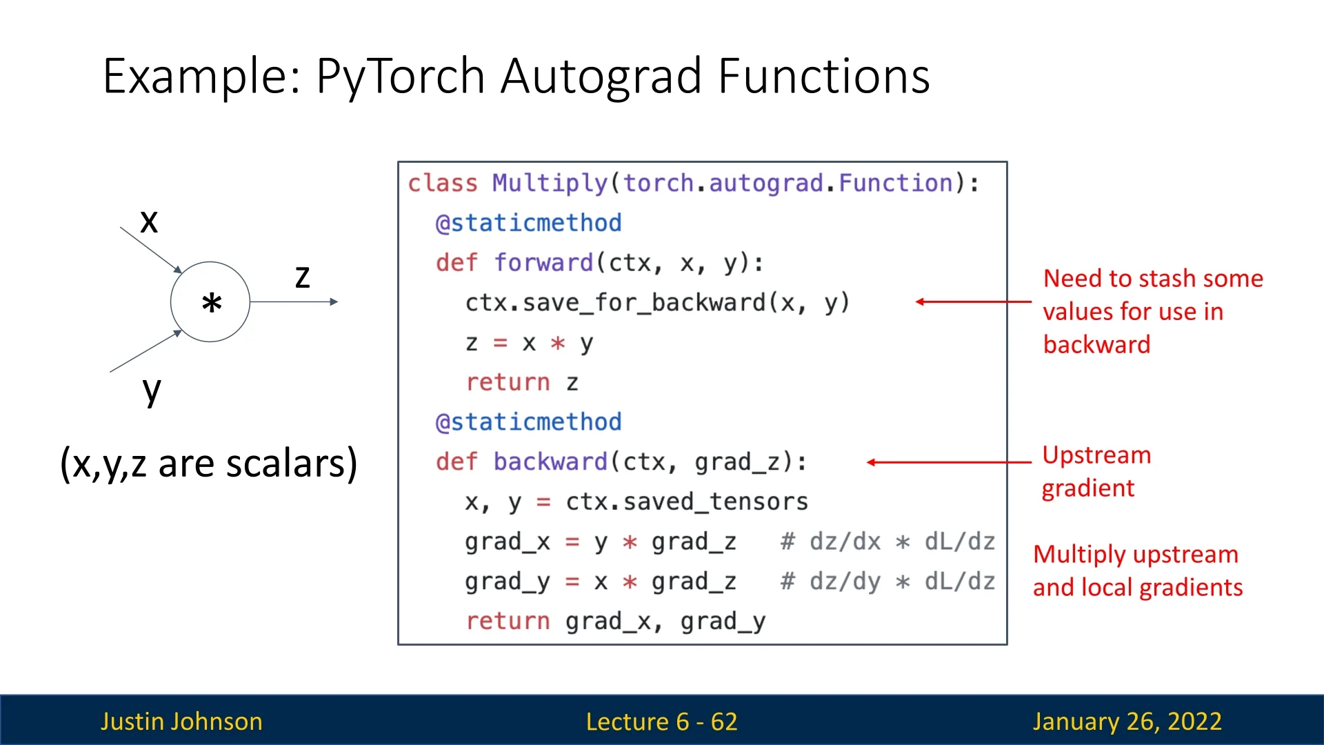
6.6.1 Example: Multiplication Gate in Autograd

Consider a simple multiplication operation \( z = x \cdot y \), implemented in PyTorch Autograd:

1.

The forward method computes \( z \) and saves \( x \) and \( y \) for the backward pass in a dedicated context variable ctx.

2.

The backward method retrieves \( x \) and \( y \) as it receives the context from the forward pass, and the upstream gradient. It then applies the chain rule, and returns the downstream gradients: \[ \frac {\partial L}{\partial x} = \frac {\partial L}{\partial z} \cdot y, \quad \frac {\partial L}{\partial y} = \frac {\partial L}{\partial z} \cdot x. \]

This pattern generalizes to all operations in a computational graph, allowing PyTorch to handle backpropagation automatically.

6.6.2 Extending Autograd for Custom Functions

Developers can extend PyTorch’s Autograd by defining their own Function classes, implementing custom forward and backward methods. By doing so, new differentiable operations can be seamlessly integrated into neural network models.

An interesting example is PyTorch’s implementation of the sigmoid activation function, which follows this modular API:

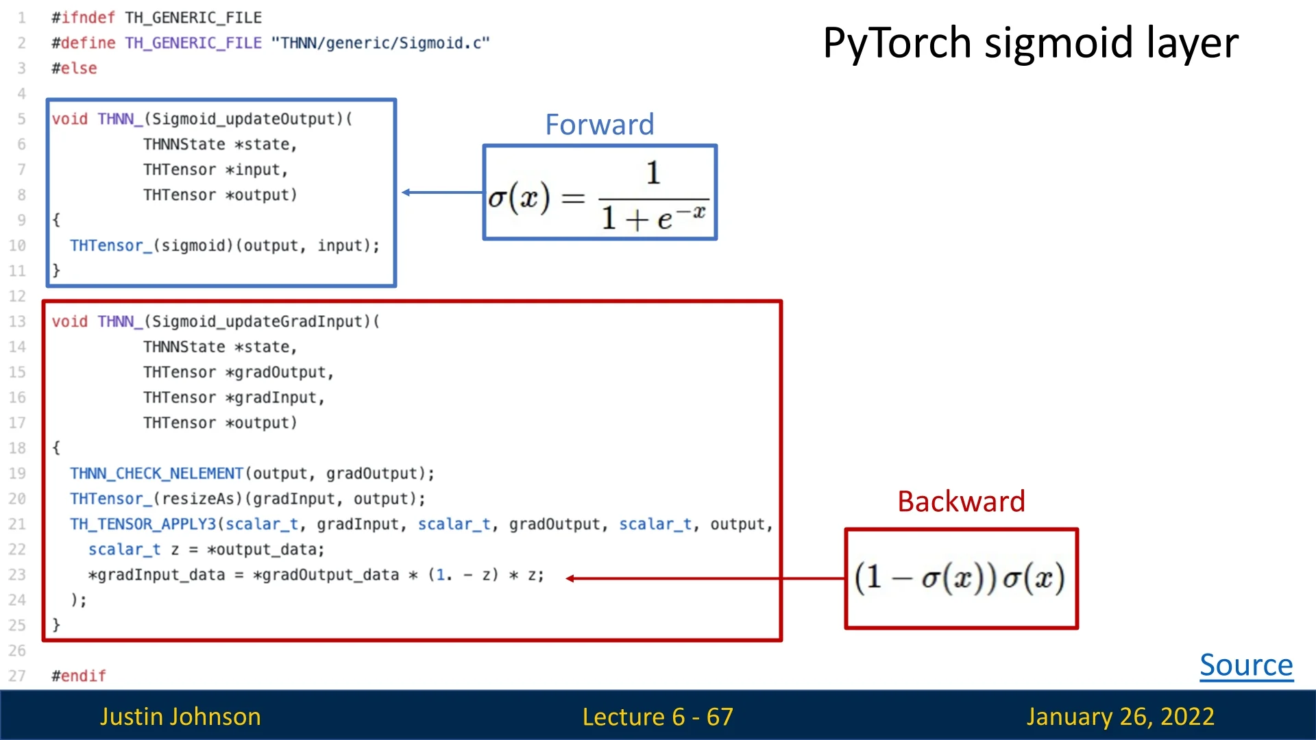
By chaining multiple such autograd functions, we construct computational graphs, enabling both inference (forward pass) and training (backward pass). This is the core essence of PyTorch.

6.7 Beyond Scalars: Backpropagation for Vectors and Tensors

So far, we have discussed backpropagation in the context of scalar-valued functions. However, real-world neural networks involve vector-valued functions, requiring us to extend backpropagation to gradients and Jacobians.

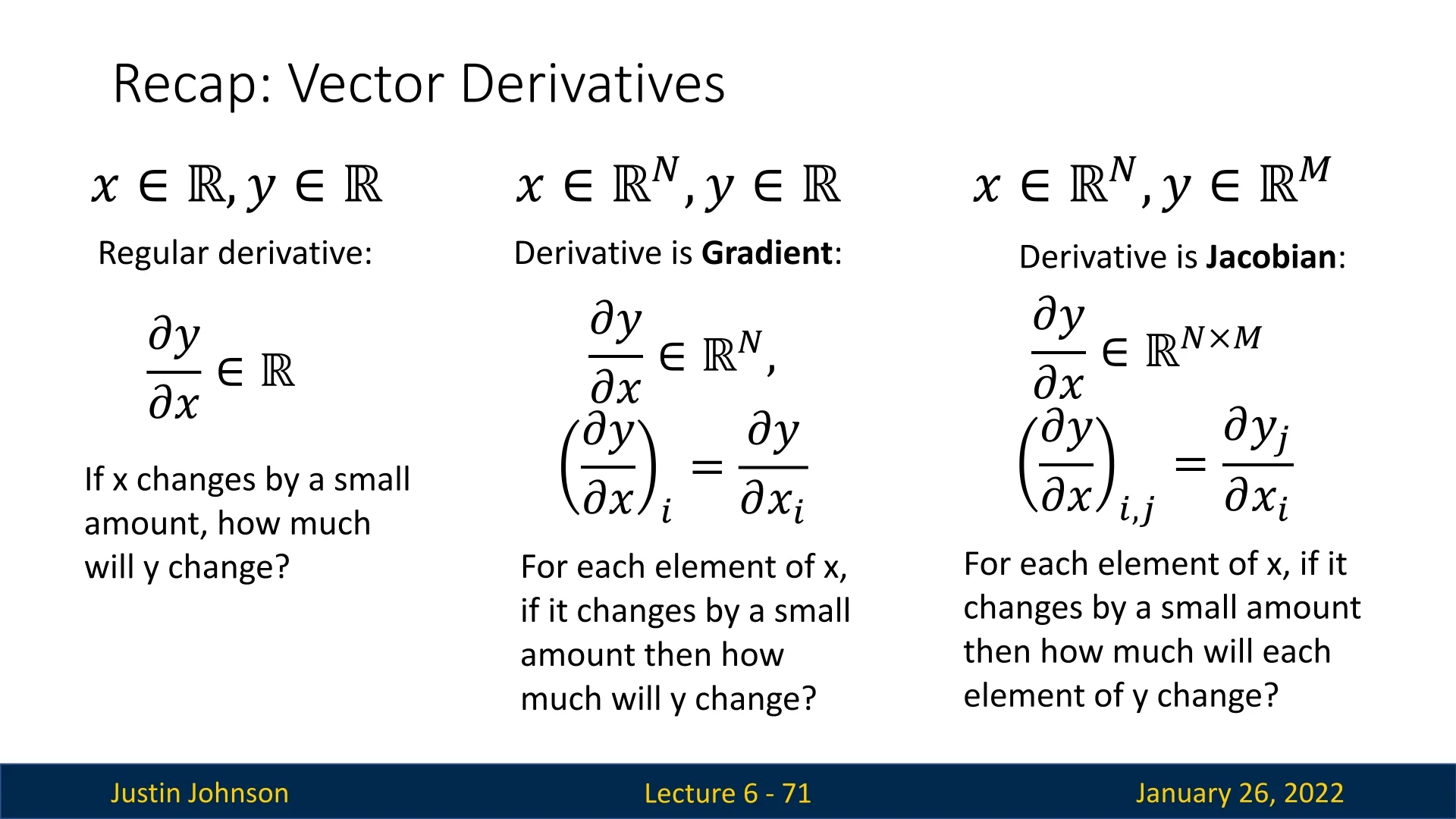
6.7.1 Gradients vs. Jacobians

• Gradient (Scalar-Valued Function): For a function \(f: \mathbb {R}^N \to \mathbb {R}\), the gradient is the vector of partial derivatives: \[ \nabla f(\mathbf {x}) \;=\; \left [ \frac {\partial f}{\partial x_1},\; \frac {\partial f}{\partial x_2},\; \dots ,\; \frac {\partial f}{\partial x_N} \right ]. \] In a typical neural network setting, \(f\) might be a loss function \(\mathcal {L}(\theta )\) of the model parameters \(\theta \), and \(\nabla \mathcal {L}\) tells us how to update the parameters to minimize the loss.
• Jacobian (Vector-Valued Function): For a function \(F: \mathbb {R}^N \to \mathbb {R}^M\), the Jacobian is an \(M \times N\) matrix where each entry \[ J_{ij} \;=\; \frac {\partial F_i}{\partial x_j} \] represents how each input dimension \(x_j\) affects each output dimension \(F_i\). Rows of this matrix can be seen as gradients of individual output components. In neural networks, this arises very often when we compute local derivatives for a node in the graph, as if the inputs to the node are vectors x, y and the output is a vector z, and each vector has its own number of elements (\(D_x, D_y, D_z\)) then the local ’gradients’ (derivatives) in this case are Jacobian matrices: dz/dx is of dim \([D_x \times D_z]\) and dz/dy is of dim \([D_y \times D_z]\).

By understanding both gradients and Jacobians, we see why backpropagation must handle vector-valued outputs (e.g., a network’s logits or output features) rather than only scalar-valued loss functions. Modern frameworks automatically compute these matrix derivatives, enabling efficient training in multi-output scenarios. We’ll now explore how the backpropagation process we’ve seen earlier generalizes to support such functions.

6.7.2 Extending Backpropagation to Vectors

In earlier sections, we focused on backpropagation when both inputs and outputs to a node were scalars. Real-world neural networks, however, typically process and produce vectors or even higher-dimensional tensors. This section provides a detailed look at how backpropagation extends to these more general scenarios.

We now move from a node that received scalars \(x, y\) and returned a scalar \(z\), to a node that handles:

• \(\mathbf {x}\in \mathbb {R}^{D_x}\) and \(\mathbf {y}\in \mathbb {R}^{D_y}\) (input vectors),
• \(\mathbf {z}\in \mathbb {R}^{D_z}\) (output vector).

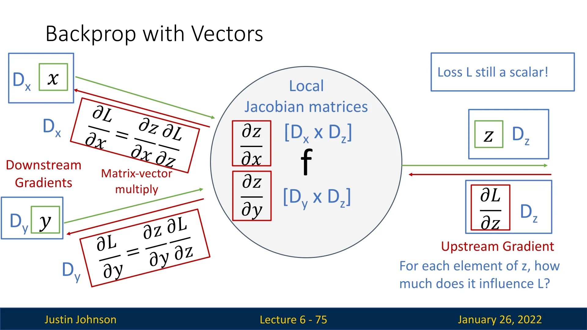
Although the output is now a vector, the overall loss function \(L\) (e.g., a training objective) remains a scalar. Therefore: \[ \underbrace {\frac {\partial L}{\partial \mathbf {z}}}_{\mbox{upstream gradient}} \in \mathbb {R}^{D_z}, \] tells us how sensitive \(L\) is to each component \(z_i\). The local gradients \(\tfrac {\partial \mathbf {z}}{\partial \mathbf {x}}\) and \(\tfrac {\partial \mathbf {z}}{\partial \mathbf {y}}\) become Jacobian matrices: \[ \frac {\partial \mathbf {z}}{\partial \mathbf {x}} \;\in \; \mathbb {R}^{D_z \times D_x}, \quad \frac {\partial \mathbf {z}}{\partial \mathbf {y}} \;\in \; \mathbb {R}^{D_z \times D_y}. \] By applying the chain rule, the downstream gradients \(\tfrac {\partial L}{\partial \mathbf {x}}\) and \(\tfrac {\partial L}{\partial \mathbf {y}}\) each become: \[ \frac {\partial L}{\partial \mathbf {x}} = \left (\frac {\partial \mathbf {z}}{\partial \mathbf {x}}\right )^\mathsf {T} \frac {\partial L}{\partial \mathbf {z}}, \qquad \frac {\partial L}{\partial \mathbf {y}} = \left (\frac {\partial \mathbf {z}}{\partial \mathbf {y}}\right )^\mathsf {T} \frac {\partial L}{\partial \mathbf {z}}, \] where each result has the same dimension as the corresponding input vector (\(D_x\) or \(D_y\)).

6.7.3 Example: Backpropagation for Elementwise ReLU

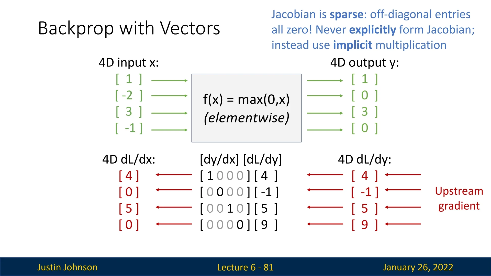
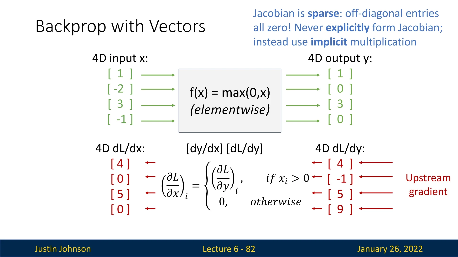
Consider an elementwise ReLU applied to a vector \(\mathbf {x}\in \mathbb {R}^{4}\). For example: \[ \mathbf {x} = \begin {bmatrix}1 \\ -2 \\ 3 \\ -1\end {bmatrix} \quad \longrightarrow \quad \mathbf {y} = \max \!\bigl (\mathbf {0},\mathbf {x}\bigr ) = \begin {bmatrix}1 \\ 0 \\ 3 \\ 0\end {bmatrix}. \] If the upstream gradient (the sensitivity of the loss \(L\) w.r.t. each element of \(\mathbf {y}\)) is \[ \frac {\partial L}{\partial \mathbf {y}} = \begin {bmatrix}4 \\ -1 \\ 5 \\ 9\end {bmatrix}, \] we must compute \(\tfrac {\partial L}{\partial \mathbf {x}}\). Conceptually, the local Jacobian \(\tfrac {\partial \mathbf {y}}{\partial \mathbf {x}}\) is a \(4\times 4\) diagonal matrix: \[ \begin {bmatrix} 1 & 0 & 0 & 0\\ 0 & 0 & 0 & 0\\ 0 & 0 & 1 & 0\\ 0 & 0 & 0 & 0 \end {bmatrix}, \] where the diagonal element is \(1\) if \(x_i>0\) and \(0\) otherwise. This multiplication yields: \[ \frac {\partial L}{\partial \mathbf {x}} = \begin {bmatrix}4 \\ 0 \\ 5 \\ 0\end {bmatrix}. \]

6.7.4 Efficient Computation via Local Gradient Slices

High-dimensional neural network operations, such as matrix multiplications or convolutions, often have massive Jacobians when viewed formally. Storing or iterating over all partial derivatives explicitly is impractical. Instead, we exploit local gradient slices to determine how each input component affects the output, then combine these slices via standard matrix multiplications.

6.7.5 Backpropagation with Matrices: A Concrete Example

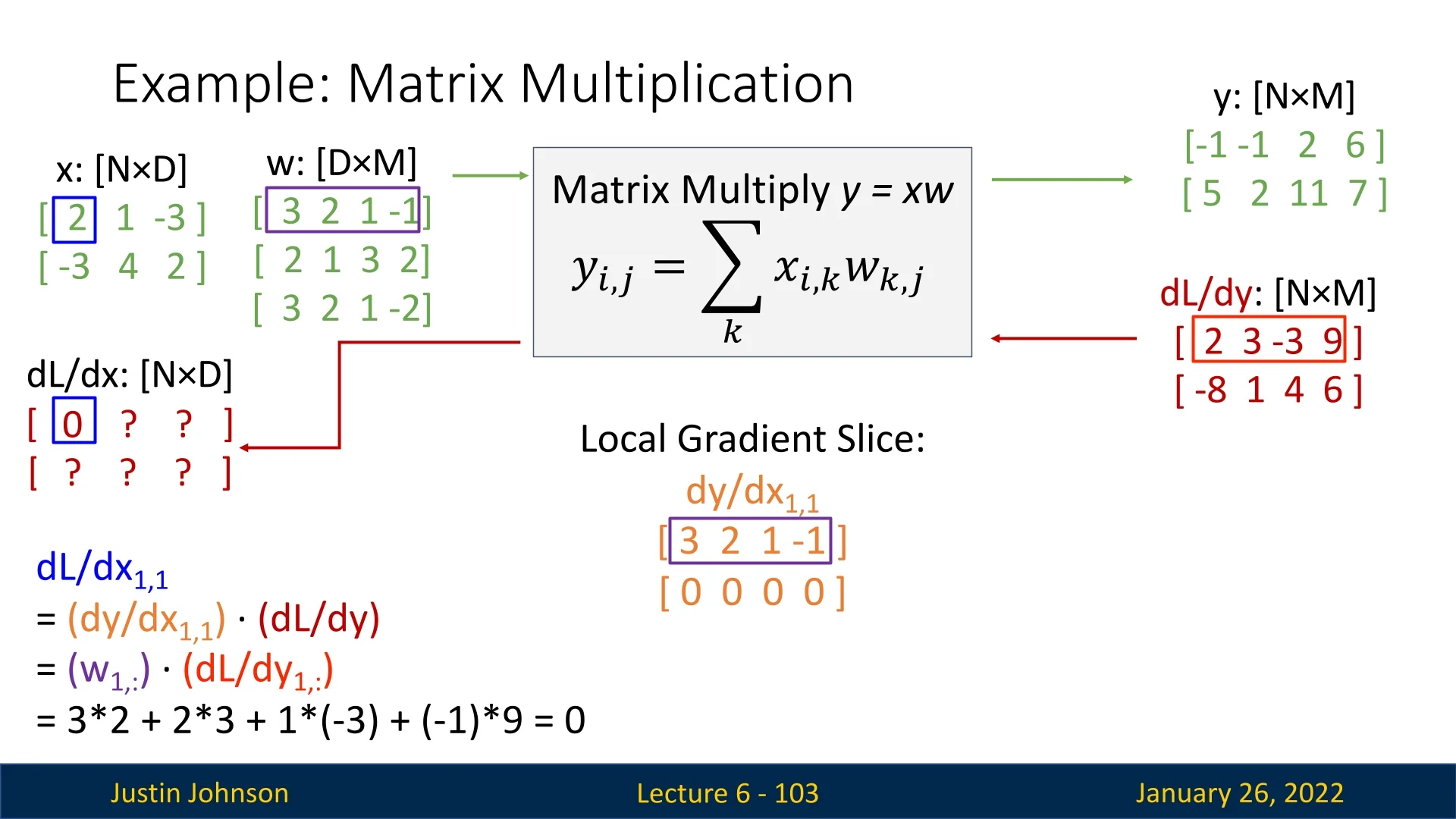
Consider a matrix multiplication: \[ \mathbf {Y} = \mathbf {X}\,\mathbf {W}, \] where \(\mathbf {X}\in \mathbb {R}^{N\times D}\), \(\mathbf {W}\in \mathbb {R}^{D\times M}\), and \(\mathbf {Y}\in \mathbb {R}^{N\times M}\). We have a scalar loss \(L\), and the upstream gradient \(\tfrac {\partial L}{\partial \mathbf {Y}}\) is also an \((N\times M)\)-shaped matrix.

Numerical Setup. Let \(N=2\), \(D=3\), and \(M=4\). Suppose: \[ \mathbf {X} = \begin {bmatrix} 2 & 1 & -3 \\ -3 & 4 & 2 \end {bmatrix}, \quad \mathbf {W} = \begin {bmatrix} 3 & 2 & 1 & -1 \\ 2 & 1 & 3 & 2 \\ 3 & 2 & 1 & -2 \end {bmatrix}. \] Multiplying gives \(\mathbf {Y}\in \mathbb {R}^{2\times 4}\). Concretely, \[ \mathbf {Y} = \mathbf {X}\,\mathbf {W} = \begin {bmatrix} -1 & -1 & 2 & 6 \\ 5 & 2 & 11 & 7 \end {bmatrix}. \] In the backward pass, we receive: \[ \frac {\partial L}{\partial \mathbf {Y}} = \begin {bmatrix} 2 & 3 & -3 & 9 \\ -8 & 1 & 4 & 6 \end {bmatrix}. \]

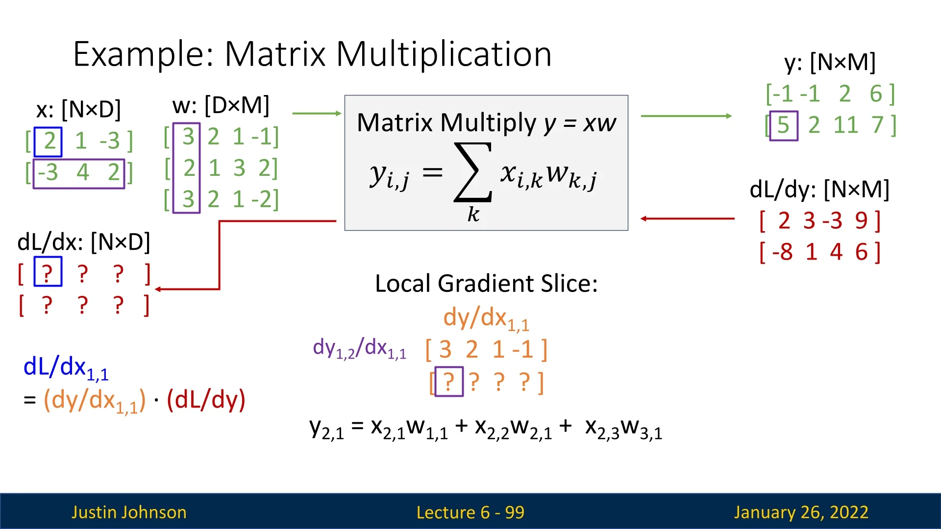
Slice Logic for One Input Element. Focusing on a single entry, e.g. \(\mathbf {X}_{1,1}=2\):

• Only row \(1\) of \(\mathbf {Y}\) depends on \(\mathbf {X}_{1,1}\).
• Each element \(y_{1,m}\) is updated by \(x_{1,1}\cdot w_{1,m}\).
• The second row \(y_{2,\cdot }\) is unaffected, so its local gradient is zero.

Hence, for \(\mathbf {X}_{1,1}\), the local gradient slice \(\tfrac {\partial \mathbf {Y}}{\partial x_{1,1}}\) has the form: \[ \begin {bmatrix} w_{1,1} & w_{1,2} & w_{1,3} & w_{1,4}\\ 0 & 0 & 0 & 0 \end {bmatrix}. \] Next, we take the elementwise product with \(\tfrac {\partial L}{\partial \mathbf {Y}}\) over the same region to compute \(\tfrac {\partial L}{\partial x_{1,1}}\). Numerically: \[ w_{1,\cdot } = [\,3,\;2,\;1,\;-1\,], \quad \frac {\partial L}{\partial y_{1,\cdot }} = [\,2,\;3,\;-3,\;9\,]. \] So \[ \tfrac {\partial L}{\partial x_{1,1}} = 3\times 2 + 2\times 3 + 1\times (-3) + (-1)\times 9 = 0. \]

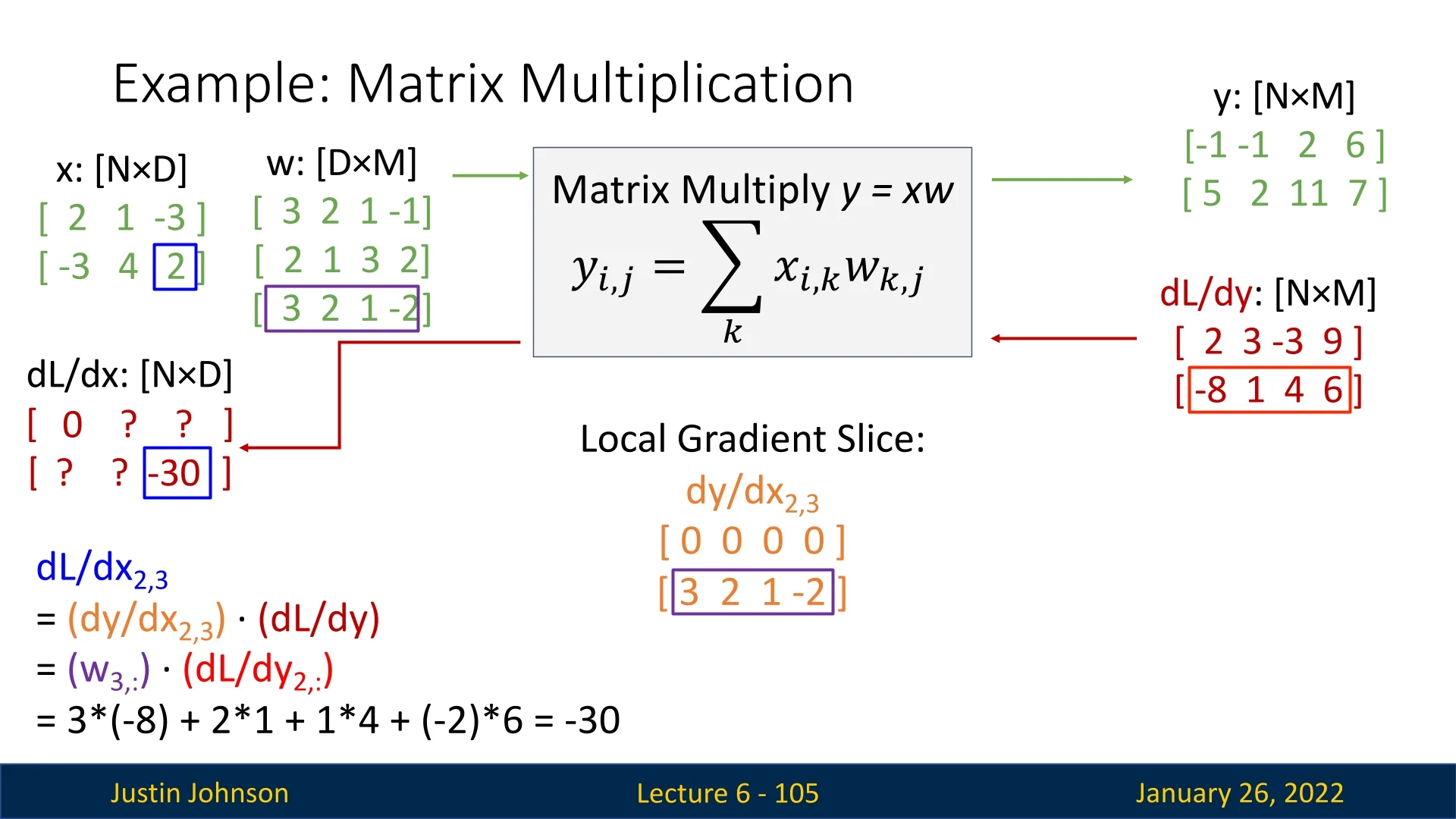
Another Example: \(\mathbf {X}_{2,3}\). For \(\mathbf {X}_{2,3}=2\):

• Only row \(2\) of \(\mathbf {Y}\) depends on it.
• Each element \(y_{2,m}\) is updated by \((x_{2,3}\cdot w_{3,m})\).
• The first row is unaffected (local gradient is zero).

If \(w_{3,\cdot } = [\,3,\;2,\;1,\;-2\,]\), then \[ \tfrac {\partial L}{\partial x_{2,3}} = 3\times (-8) + 2\times 1 + 1\times 4 + (-2)\times 6 = -24 + 2 + 4 - 12 = -30. \]

6.7.6 Implicit Multiplication for the Entire Gradient

While the slice-by-slice perspective shows how each input entry influences each output entry, in practice we combine all slices at once with matrix multiplication. Concretely: \[ \frac {\partial L}{\partial \mathbf {X}} = \left (\frac {\partial L}{\partial \mathbf {Y}}\right ) \,\mathbf {W}^\mathsf {T}, \quad \frac {\partial L}{\partial \mathbf {W}} = \mathbf {X}^\mathsf {T} \,\left (\frac {\partial L}{\partial \mathbf {Y}}\right ). \] These expressions produce the exact same result as summing the contributions from each local slice individually—without constructing the full \(((N\times D)\times (N\times M))\) Jacobian.

Why Slices Are the Solution.

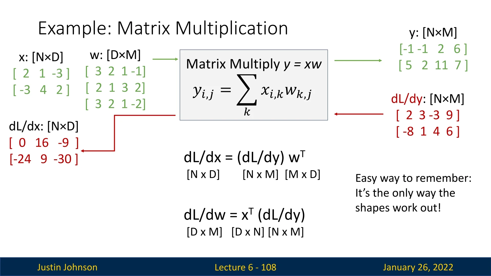
• Memory Savings: Instead of building a giant Jacobian, we focus on local slices (each shaped like \(\mathbf {Y}\), and effectively, a row of \(\mathbf {Y}\) that is not 0s) and multiply them with the matching row of \(\tfrac {\partial L}{\partial \mathbf {Y}}\) to get the corresponding element of the downstream gradient. The local slices can be discarded each time after we finish the computation of the corresponding element of the downstream gradient.
• Efficiency: In practice, we skip per-element slicing entirely and jump to \(\bigl (\tfrac {\partial L}{\partial \mathbf {Y}}\bigr )\,\mathbf {W}^\mathsf {T}\) and \(\mathbf {X}^\mathsf {T}\,\bigl (\tfrac {\partial L}{\partial \mathbf {Y}}\bigr )\) using fast BLAS/GPU kernels.
• Scalability to High Dimensional Tensors: For high-rank tensors (e.g., images), the same principle applies. We typically flatten or reshape dimensions to perform the relevant multiplications in a similarly efficient manner.

This implicit backprop approach avoids the exponential growth of explicit Jacobian storage, making gradient-based learning feasible even for large-scale neural networks.

6.7.7 A Chain View of Backpropagation

Another way to understand backpropagation is to see the computational graph as a chain of functions operating on intermediate variables. Suppose we have: \[ x_1 = f_1(x_0), \quad x_2 = f_2(x_1), \quad \dots , \quad L = f_4(x_3), \] where \( f_4 \) outputs the scalar loss \( L \). This chain perspective is especially useful when exploring different modes of automatic differentiation.

Reverse-Mode Automatic Differentiation

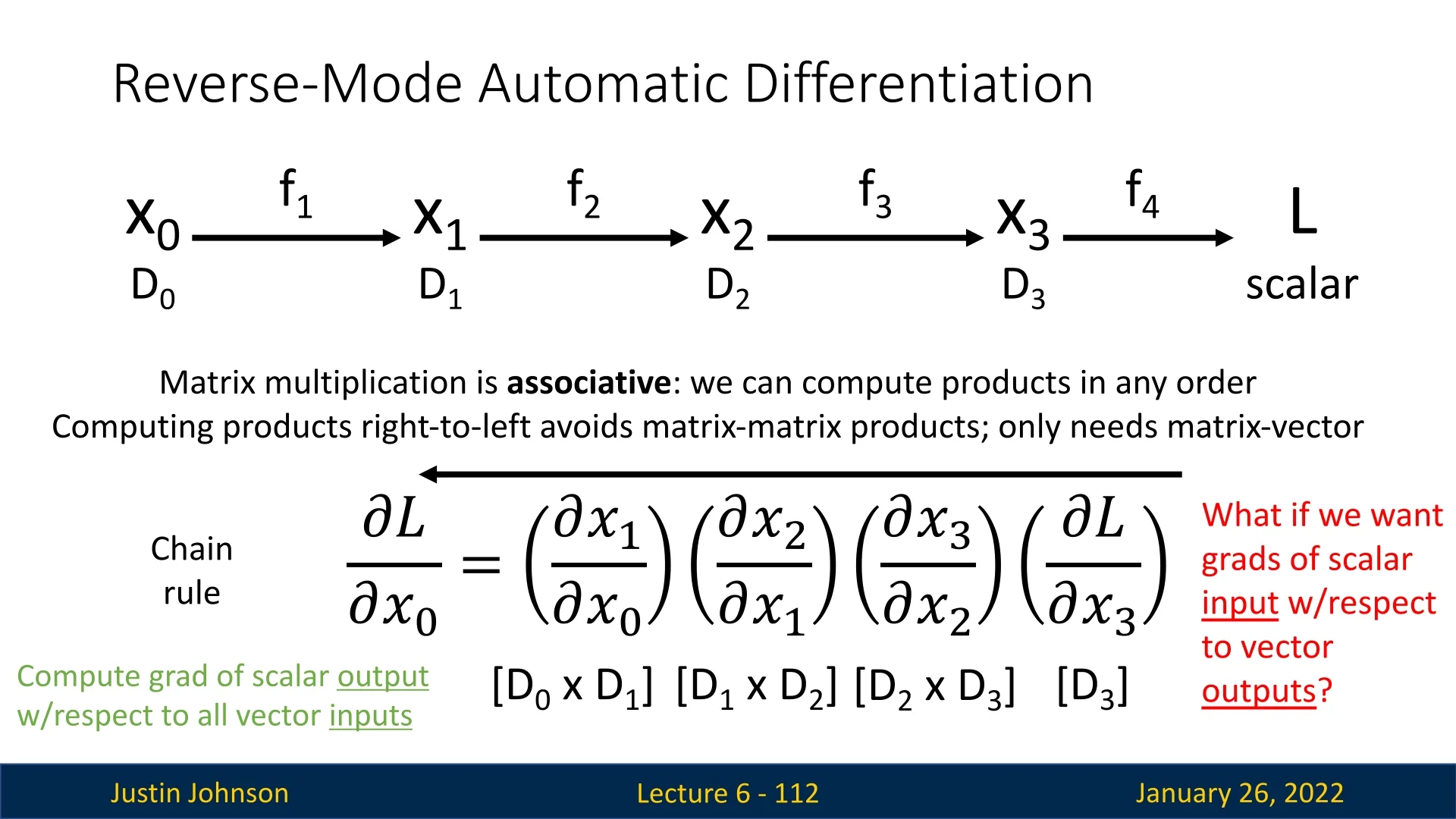
When a scalar loss \(L\) appears at the end of the computational graph, reverse-mode automatic differentiation efficiently calculates gradients with respect to a large number of parameters. By traversing the chain from \(L\) backward, matrix-vector products replace matrix-matrix products, which is much more efficient for high-dimensional problems.

Forward-Mode Automatic Differentiation

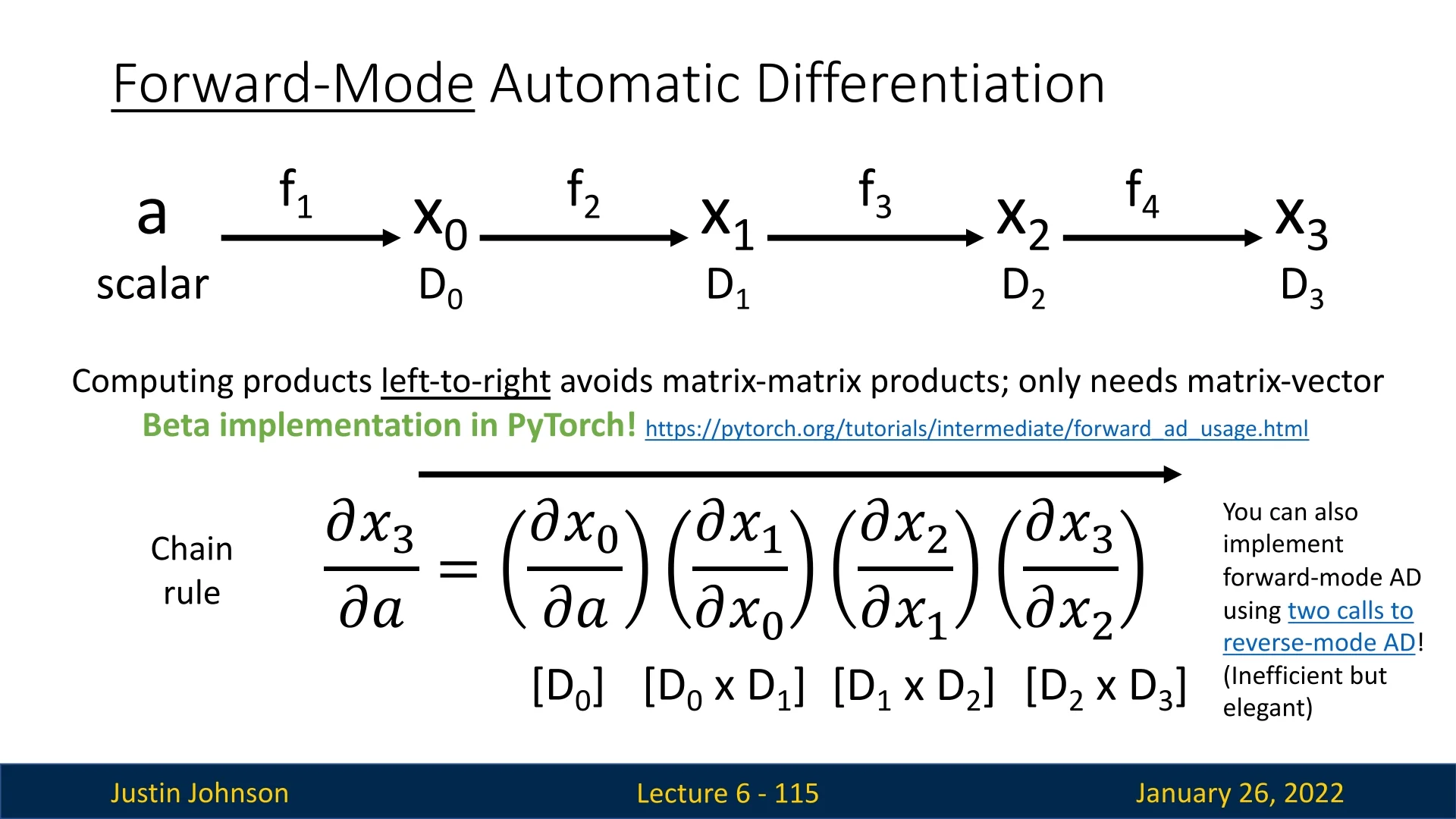
In contrast to reverse-mode automatic differentiation, which is optimized for computing derivatives of a scalar loss with respect to many parameters, forward-mode automatic differentiation is more suitable when:

• A single scalar input (or a few inputs) affects many outputs, and we need derivatives of all outputs with respect to this input.
• The computational graph is narrow but deep (e.g., computing derivatives with respect to time-dependent variables in simulations).

When Is Forward-Mode Automatic Differentiation is Useful? While forward-mode differentiation is rarely used in deep learning, it plays a crucial role in other scientific and engineering domains, including:

• Physics Simulations: Understanding how changes in fundamental constants (e.g., gravity, friction) affect entire system dynamics.
• Sensitivity Analysis: Evaluating how small variations in input parameters propagate through a model, which is essential for robust system design.
• Computational Finance and Engineering: Where derivative calculations are needed for risk modeling and structural analysis.

Unlike reverse-mode differentiation, which propagates gradients backward, forward-mode propagates derivatives forward through the computation graph, making it efficient for computing derivatives with respect to a few key inputs.

6.7.8 Computing Higher-Order Derivatives with Backpropagation

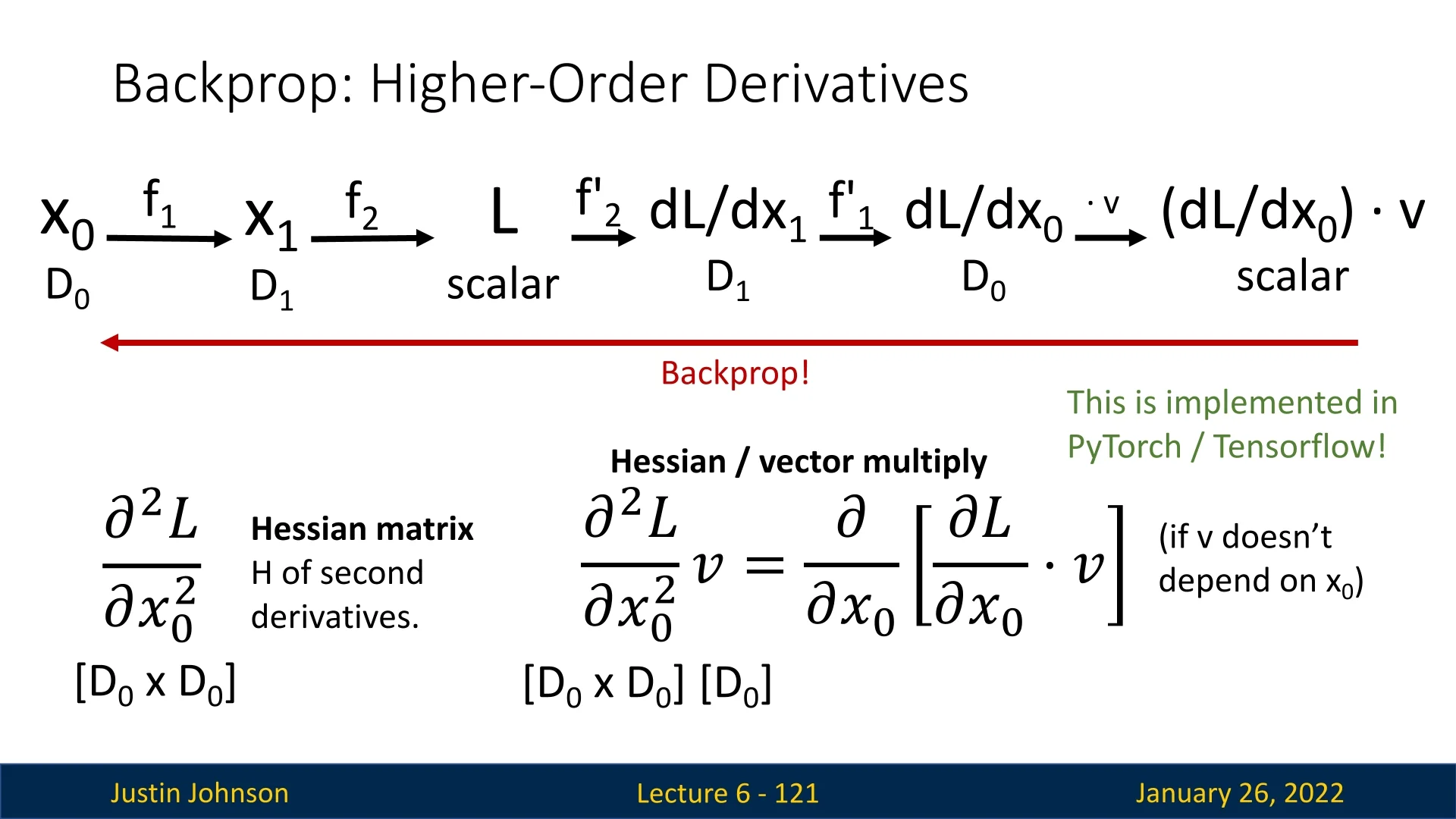
So far, we have focused on first-order derivatives, which capture how small changes in parameters affect the loss function. However, higher-order derivatives, such as Hessians (matrices of second-order partial derivatives), provide additional insights.

Why Compute Hessians? The Hessian matrix \( \mathbf {H} = \nabla ^2 L \) captures second-order effects, helping in:

• Second-Order Optimization: Methods like Newton’s method and quasi-Newton methods (e.g., L-BFGS) use Hessian information for faster convergence.
• Understanding Model Sensitivity: Hessians quantify how different parameters interact and influence optimization.
• Regularization and Pruning: Hessian-based techniques help in feature selection and gradient-based network pruning.

Efficient Hessian Computation: Hessian-Vector Products A naive approach to computing the Hessian matrix explicitly is infeasible in large-scale models (as it requires storing an \( \mathbb {R}^{N \times N} \) matrix). Instead, we use Hessian-vector multiplication: \[ \mathbf {H} \mathbf {v} = \nabla \left ( \nabla L \cdot \mathbf {v} \right ), \] which allows us to obtain second-order information efficiently without forming the full Hessian matrix.

6.7.9 Application: Gradient-Norm Regularization

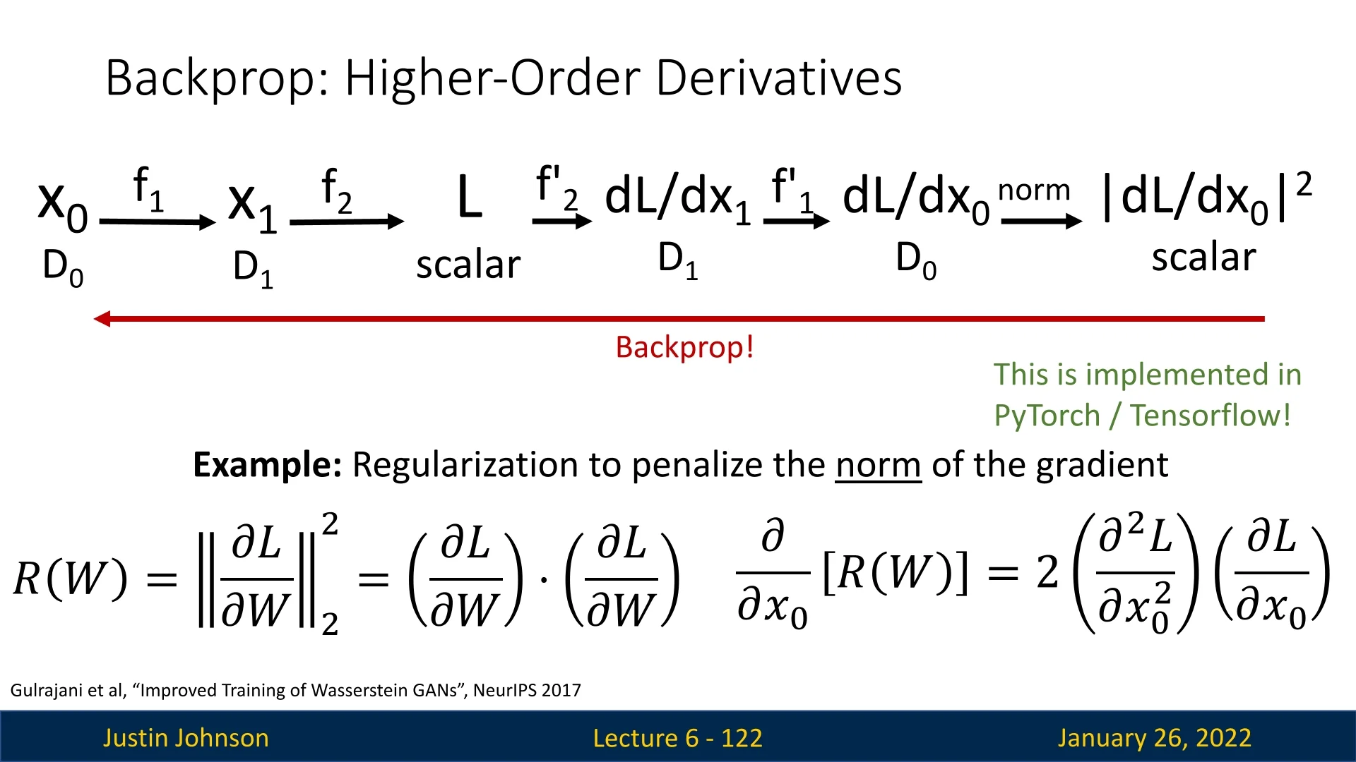
One practical application of higher-order derivatives in deep learning is penalizing the gradient norm: \[ R(W) = \|\nabla _W L\|_2^2. \] Computing \( \tfrac {d}{d W}R(W) \) involves second derivatives of \( L \). With backpropagation for higher-order terms, we can approximate or compute this regularization effectively, potentially improving model training by smoothing out rugged loss landscapes.

6.7.10 Automatic Differentiation: Summary of Key Insights

Automatic differentiation (AD) provides a unified framework for efficiently computing derivatives of complex functions expressed as computational graphs. Backpropagation, as used in deep learning, is a specific instance of this framework—corresponding to reverse-mode automatic differentiation.

• Reverse-mode automatic differentiation (backpropagation). In deep learning, we typically minimize a scalar loss with respect to millions of parameters. Reverse-mode AD propagates sensitivities backward through the computational graph, allowing all partial derivatives of a scalar output to be computed in a single backward pass. This makes it the method of choice for large-scale neural network training.
• Forward-mode automatic differentiation. Forward-mode AD pushes derivatives forward from the inputs instead of backward from the output. It is most efficient when there are few input variables but many outputs—such as in scientific computing, sensitivity analysis, and physical simulations—where the goal is to measure how a single parameter affects multiple outcomes.
• Higher-order derivatives. The same computational principles that underlie backpropagation can be extended to compute higher-order derivatives, including Hessians and Hessian–vector products. These quantities capture curvature information, enabling more refined optimization strategies.
• Second-order methods and regularization. Hessian-based quantities support advanced techniques such as second-order optimization (e.g., Newton’s method) and curvature-aware regularization, which can improve convergence speed and stability in challenging loss landscapes.

Taken together, these insights highlight that backpropagation is not merely a training algorithm, but a powerful instance of the broader concept of automatic differentiation. The same underlying ideas—propagating derivatives through computational graphs—form the mathematical foundation for a wide spectrum of applications, from deep learning optimization to scientific modeling and engineering simulations.