Lecture 22: Self-Supervised Learning
22.1 Motivation and Definition
22.1.1 What is Self-Supervised Learning (SSL)?
Learning Representations Without Labels Self-Supervised Learning (SSL) is a learning paradigm that allows models to learn from unlabeled data by solving automatically constructed tasks—known as pretext tasks—that do not require manual annotations. These tasks are derived from the raw input itself and are carefully designed to encourage the model to learn semantic structure and meaningful features that transfer well to standard supervised tasks such as image classification, object detection, or segmentation.
A central goal in SSL is to obtain a compact embedding function \[ f_\theta : \mathbb {R}^D \rightarrow \mathbb {R}^d, \qquad \mbox{where} \quad d \ll D, \] that maps high-dimensional inputs (e.g., images) to low-dimensional feature vectors. These embeddings should reflect the intrinsic structure of the data: semantically similar inputs (e.g., two views of the same object) should have high similarity in the latent space, while dissimilar inputs should be mapped far apart. This geometric constraint is typically imposed using a distance metric such as cosine similarity or Euclidean distance.
Pretraining Then Transferring Most SSL pipelines follow a two-stage workflow:
- 1.
- Pretraining: The model is trained from scratch to solve a synthetic pretext task using only unlabeled data. This forces the encoder to develop robust, general-purpose features.
- 2.
- Transfer: The learned encoder is then adapted to a downstream task. This can be done by fine-tuning all weights using a small amount of labeled data, or by freezing the encoder and training only a lightweight head (e.g., a linear classifier).
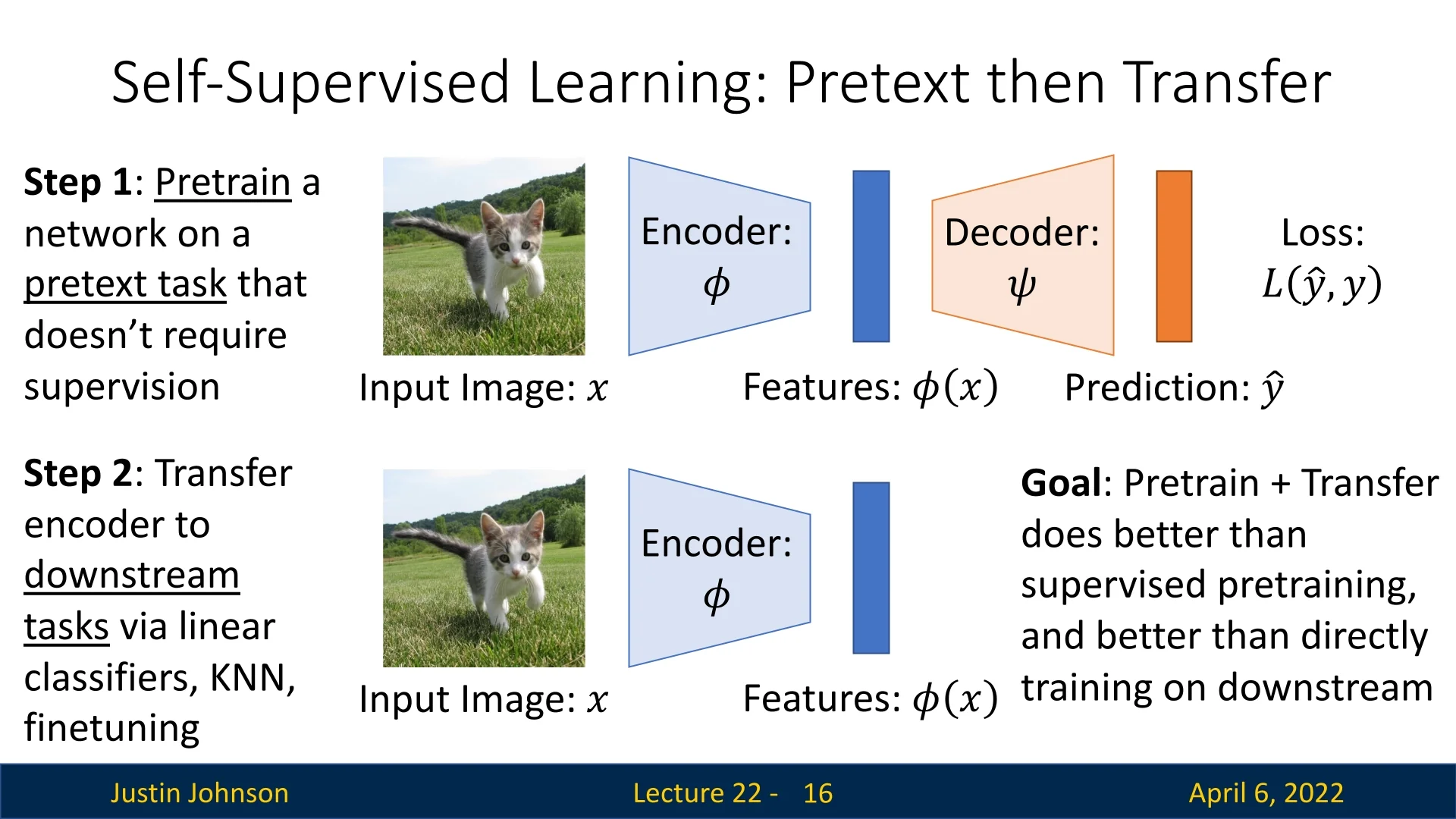
This two-phase approach is illustrated in Figure 22.1. Notably, SSL-based pretraining can outperform both randomly initialized models and models trained in a fully supervised manner on large-scale labeled datasets such as ImageNet—especially when downstream labels are scarce.
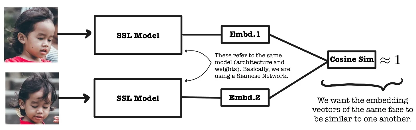
Embedding Geometry and Semantic Similarity At the heart of SSL is the idea of embedding structure. The model is encouraged to produce similar embeddings for input samples that are semantically related (e.g., different augmentations of the same image), while enforcing dissimilarity between unrelated examples. This results in a representation space in which similarity under a fixed metric (such as cosine similarity) reflects semantic closeness. In many cases, the learned embeddings can serve directly as features for classification, retrieval, or verification.
Why Pretext Tasks Work Although pretext tasks may appear synthetic or even trivial in nature, their solutions often require understanding of high-level structure and semantics. For example, a task that involves predicting the correct orientation of an image implicitly forces the model to recognize objects and their canonical alignment. Similarly, tasks that rely on partial reconstruction require capturing texture, geometry, and context. By solving such surrogate tasks, the model acquires transferable visual concepts that generalize well across datasets and tasks.
Categories of Pretext Tasks Pretext tasks vary in their construction, but all share the goal of inducing the model to learn informative and transferable features. They can be grouped into several broad categories:
-
Generative tasks: These involve reconstructing or generating parts of the input image:
- Autoencoding: Compress and reconstruct the original image.
- Denoising / Masked Modeling [219]: Predict masked or corrupted image regions.
- Colorization [799]: Recover color from grayscale inputs.
- Inpainting [486]: Fill in missing patches.
- Autoregressive prediction: Predict future pixels or patches based on context.
- Generative Adversarial Training [186]: Learn to synthesize realistic images.
-
Discriminative tasks: These involve predicting a categorical property or relation:
- Context prediction [131]: Identify the relative spatial layout of image patches.
- Rotation prediction [178]: Classify the discrete rotation applied to an image.
- Clustering and pseudo-labeling [69]: Assign images to unsupervised feature clusters.
- Similarity discrimination [89, 220]: Distinguish between similar and dissimilar inputs.
-
Multimodal tasks: These extend SSL beyond RGB by incorporating other input modalities:
Backbones, Augmentations, and Losses The success of SSL depends not only on the task formulation but also on architectural and algorithmic choices. Backbone networks such as ResNets [215] and Vision Transformers [134] are commonly used to extract hierarchical features. Data augmentations—such as cropping, flipping, color jittering, and blurring—play a critical role in enforcing invariance and robustness by creating diverse input views. Loss objectives vary by task type and are tailored to align representations appropriately; further details are introduced later in this chapter.
Summary Self-supervised learning enables models to learn visual representations by solving data-derived pretext tasks. These representations, encoded as compact embeddings, exhibit semantic structure and generalize across tasks and domains. SSL has emerged as a foundational paradigm for scalable learning in the absence of labels.
22.1.2 Why Self-Supervised Learning?
Supervised Learning is Expensive Modern deep learning systems thrive on data—but high-quality labeled datasets are costly to obtain at scale. Consider the task of labeling one billion images: even under optimistic assumptions (10 seconds per image, a wage of $15/hour), the annotation cost exceeds $40 million. This estimate excludes setup overheads, platform fees, and quality control, meaning real-world costs could easily be two to three times higher. As models grow larger and more data-hungry—such as Vision Transformers and foundation models—this dependency on human-annotated supervision becomes increasingly impractical.
But Unlabeled Data is Free (and Plentiful) In contrast, unlabeled image data is ubiquitous. Vast corpora of raw images can be harvested from the web, videos, or embedded sensors at minimal cost. Self-Supervised Learning (SSL) capitalizes on this abundance by creating artificial supervision signals from the data itself. Rather than relying on manually assigned class labels, SSL constructs pretext tasks—auxiliary objectives that encourage the model to uncover meaningful structures within the input.
Learning Like Humans Unlike traditional supervised systems, human learning is largely unsupervised. Babies are not handed millions of labeled examples—instead, they learn by interacting with their environment, forming expectations, and detecting patterns. SSL adopts a similar philosophy: it trains models to predict naturally occurring signals in the input (e.g., spatial context, color, motion, or other parts of the image), enabling them to develop internal representations that generalize across tasks.
SSL as the Backbone of Foundation Models This learning paradigm has enabled the emergence of powerful generalist systems, such as foundation models in vision and language. For example, CLIP [512] learns visual representations by aligning images with their associated captions—without requiring fine-grained category labels. Inspired by the success of large-scale self-supervised pretraining in NLP (e.g., GPT [59]), these models rely on SSL objectives—such as contrastive learning, masked prediction, or multimodal alignment—to learn semantically rich, transferable features. As a result, SSL is now a key pillar in scaling visual learning beyond the limits of supervision.
22.1.3 LeCun’s AI Cake: SSL as the Base Layer
The Cake Analogy Yann LeCun famously likened the components of AI to a layered cake:
- Génoise (Base): Self-Supervised Learning—general representation learning from unlabeled data.
- Icing: Supervised Learning—fine-tuning on specific tasks with labeled data.
- Cherry: Reinforcement Learning—learning from sparse reward signals in sequential decision tasks.
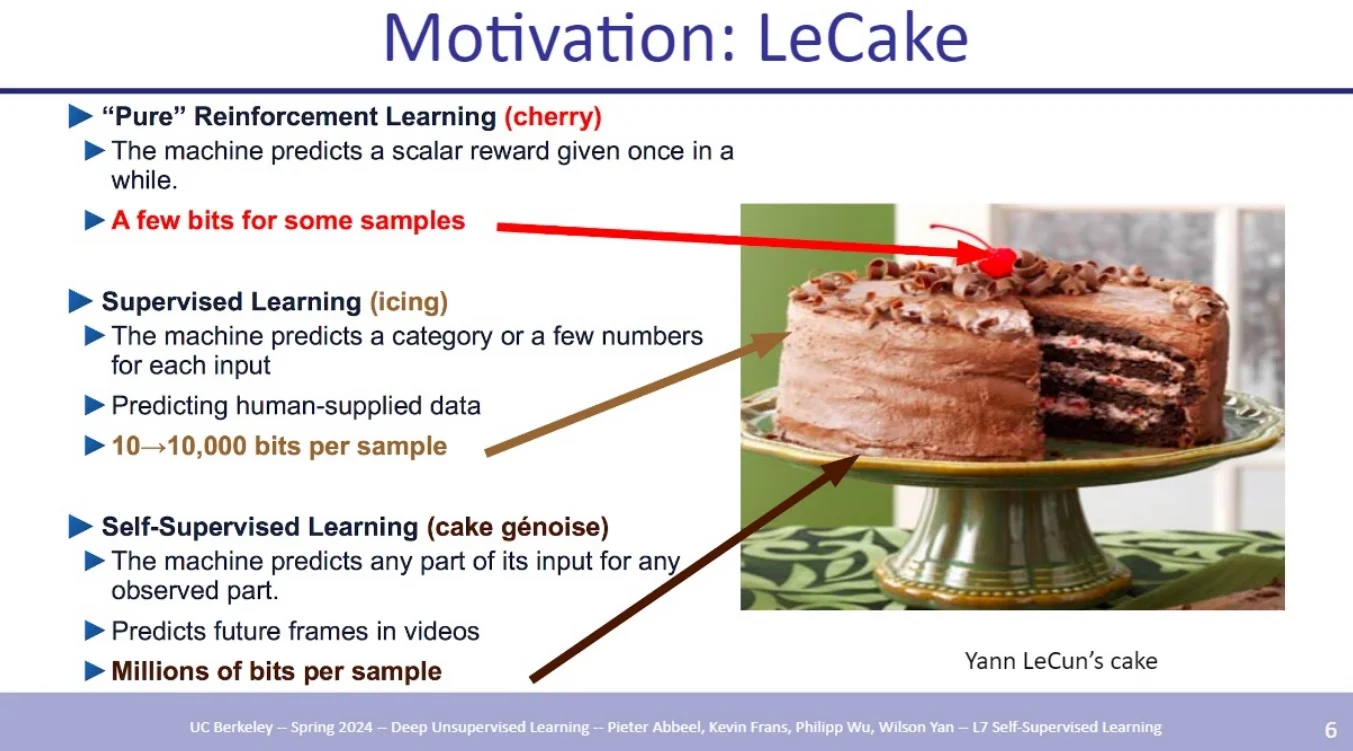
Practical Significance This analogy underscores that any intelligent pipeline should begin with SSL to form robust foundational knowledge before adding task-specific or behavior-based learning.
22.1.4 Practical Integration into Deep Learning Pipelines
How SSL is Used in Practice SSL models are often trained on vast unlabeled datasets to produce strong feature extractors. These are then reused in downstream tasks:
- Linear classifiers for probing representation quality.
- KNN retrieval to test neighborhood consistency.
- MLPs for non-linear transfer to downstream tasks.
- Fine-tuning the backbone network on task-specific data.
Flexible Transfer and Modularity In practice, a lightweight classifier—typically a linear layer or a shallow multilayer perceptron (MLP)—is attached on top of the frozen encoder to perform downstream tasks. If the learned representations are not perfectly linearly separable, using an MLP head with 2–3 layers often yields substantial performance improvements by capturing mild nonlinearities.
Full fine-tuning of the encoder is also possible and sometimes beneficial when ample downstream labels are available. However, this approach introduces significantly more trainable parameters and risks overfitting in low-data regimes. As such, full fine-tuning should be reserved for downstream datasets of moderate to large scale, while smaller datasets benefit more from frozen representations with minimal adaptation.
Strategic Impact and Adoption Self-supervised learning has become the default pretraining strategy for modern vision models, particularly large-scale architectures like Vision Transformers. By eliminating the need for manual annotation, SSL shifts the bottleneck from label curation to scalable data collection, enabling broader and more cost-effective deployment. Its ability to learn transferable features from unlabeled data makes it a foundational component of contemporary AI pipelines.
22.2 A Taxonomy of Self-Supervised Representation Learning Methods
Self-Supervised Representation Learning (SSRL) now comprises a diverse set of methods that extract meaningful representations from unlabeled data. These methods are generally categorized into four principal families based on their core learning strategies.
22.2.1 Contrastive Methods
Discriminative Representations via Similarity and Dissimilarity Contrastive approaches train encoders to pull together representations of similar samples (positive pairs) and push apart those of dissimilar ones (negative pairs). These typically rely on aggressive data augmentation and clever mining or sampling strategies.
- SimCLR / SimCLR v2 [89, 90]: Frameworks that rely on strong augmentations and a projection head; SimCLR v2 adds depth and fine-tuning.
- MoCo / MoCo v2 / MoCo v3 [220, 96, 95]: Momentum Contrast methods with a dynamic dictionary and momentum encoder; v2 improves augmentations and projection design, v3 applies them to ViTs.
- ReLIC / ReLIC v2 [450, 640]: Contrastive methods that extend instance discrimination with latent clusters.
- CLIP [512]: Multimodal contrastive learning aligning image and text embeddings.
- NNCLR [139]: Nearest-neighbor based contrastive learning for representation smoothing and consistency.
Insight Contrastive methods achieve strong performance but often require large batch sizes, memory banks, or additional sampling heuristics to mine hard negatives.
22.2.2 Distillation-Based Methods
Teacher-Student Framework without Negatives Distillation-based approaches avoid negative samples by training a student network to match the embeddings or output distributions of a slowly-updated teacher model.
- BYOL [194]: Learns representations by aligning student and teacher networks without any contrastive negatives.
- SimSiam [93]: Demonstrates that negative samples and momentum encoders are not strictly required.
- DINO / DINOv2 [71, 477]: Combines ViT architectures with self-distillation, yielding highly transferable visual features.
- C-BYOL [330]: Introduces curriculum learning into the BYOL pipeline to improve robustness.
Insight These methods are empirically robust, especially when combined with ViT backbones, and combat representation collapse using asymmetric loss structures or architectural regularization.
22.2.3 Feature Decorrelation Methods
Promoting Redundancy Reduction These methods encourage feature dimensions to be uncorrelated, ensuring each encodes distinct information.
- Barlow Twins [774]: Minimizes off-diagonal cross-correlations while aligning features.
- VICReg [27]: Combines variance preservation with invariance and decorrelation terms.
- TWIST [146]: Adds whitening-based losses atop Barlow-style objectives to enhance decorrelation.
Insight By enforcing statistical independence across channels, these approaches reduce collapse risk and yield more disentangled representations.
22.2.4 Clustering-Based Methods
Learning via Group-Level Semantics Clustering-based approaches group similar samples using pseudo-labels from online or offline clustering, and then train the model to predict cluster assignments.
- DeepCluster / DeeperCluster [69, 73]: Alternate between k-means clustering and training the network using cluster assignments.
- SwAV [72]: Learns cluster prototypes and aligns augmentations via swapped prediction.
Insight These methods bridge the gap between contrastive and generative modeling, capturing semantic structure without explicit supervision or handcrafted positives/negatives.
Summary Table
| Category | Key Mechanism | Representative Methods |
|---|---|---|
| Contrastive | Pull together similar samples; repel negatives using contrastive losses | SimCLR, MoCo, CLIP, ReLIC, ReLICv2, NNCLR |
| Distillation | Match teacher and student outputs via EMA; no negatives needed | BYOL, SimSiam, DINO, DINOv2, C-BYOL |
| Feature Decorrelation | Enforce uncorrelated dimensions via covariance-based losses | Barlow Twins, VICReg, TWIST |
| Clustering | Use pseudo-labels from clustering to form supervision | DeepCluster, SwAV, DeeperCluster |
22.3 Contrastive Methods
22.3.1 Motivation for Contrastive Learning
Among various SSL strategies, contrastive learning has emerged as a particularly effective and conceptually elegant approach for acquiring rich and transferable visual representations.
A central objective in SSL is to train a model that maps high-dimensional data (e.g., images in \( \mathbb {R}^D \)) into compact, semantically meaningful embeddings in a lower-dimensional space \( \mathbb {R}^d \), where \( d \ll D \). These embeddings are intended to satisfy a key geometric property: inputs that are semantically similar should have representations that are close under a chosen similarity metric (typically cosine similarity), while dissimilar inputs should be mapped far apart. Such semantic alignment in the embedding space enables generalization across a wide range of downstream tasks, including classification, retrieval, and segmentation.
Core Idea Contrastive learning formalizes representation learning as a discrimination problem in the latent space. The model is trained using positive pairs—typically two different augmentations of the same image—and negative pairs, composed of unrelated images. The objective is to pull positive pairs close together in the embedding space while pushing negative pairs apart. This dynamic creates a structured feature space where semantic similarity correlates with geometric proximity.
A widely used formulation is based on the contrastive loss, such as InfoNCE [473], which minimizes the distance between an anchor and its positive key, while simultaneously maximizing the distance to negative keys in a batch or memory bank. Mathematically, for an anchor representation \( z_i \) and its positive counterpart \( z_j \), the loss takes the form: \[ \mathcal {L}_{\mbox{InfoNCE}} = -\log \frac {\exp (\mbox{sim}(z_i, z_j)/\tau )}{\sum _{k=1}^{K} \exp (\mbox{sim}(z_i, z_k)/\tau )}, \] where \( \mbox{sim}(\cdot , \cdot ) \) denotes cosine similarity and \( \tau \) is a temperature hyperparameter.
Instance Discrimination as a Pretext Task Unlike traditional classification, contrastive learning does not assume predefined categories. Instead, it adopts the instance discrimination paradigm, treating each image as its own class. The model learns to identify an augmented view of the same instance among a set of distractors. This formulation naturally addresses the representation collapse problem—where a model maps all inputs to the same point—by requiring the network to maintain distinctiveness across a large set of negatives.
For instance, we can decide that given a batch of \( N \) images, each image is augmented twice to produce \( 2N \) views. These are embedded via an encoder and normalized into unit vectors. The resulting \( 2N \) representations define \( N \) positive pairs and \( 2(N-1) \) negatives per anchor. Contrastive loss is then applied over these structured pairs to enforce the desired geometry of the representation space.
Avoiding Trivial Solutions One of the key advantages of contrastive learning over earlier heuristic pretext tasks (e.g., jigsaw puzzles, rotation prediction, or colorization) is its robustness to degenerate solutions. Pretext tasks based on fixed prediction targets often result in overly task-specific or low-level features. In contrast, contrastive methods build representations through relational signals—similarity between instances—thereby capturing high-level invariances and semantic content. The explicit use of negatives ensures that the encoder cannot collapse all embeddings into a trivial constant vector.
Scalability and Generalization Contrastive methods scale effectively to large datasets and can leverage high-capacity models, such as ResNet or Vision Transformers (ViTs), to learn expressive features. Large batch sizes or memory banks are often used to provide a diverse pool of negatives, although variants have also been developed to operate efficiently under smaller memory or compute budgets.
The learned representations exhibit strong transferability and often rival or surpass those obtained through supervised pretraining. Notable examples include:
- Face verification [572], where contrastive loss enables identity-preserving embeddings for recognition and clustering.
- Zero-shot classification with CLIP [512], which learns aligned embeddings for images and natural language descriptions via contrastive training, unlocking powerful cross-modal generalization.
- General-purpose pretraining, where contrastive methods such as SimCLR [89] and MoCo [220] have closed the performance gap between supervised and self-supervised approaches across many vision benchmarks.
Key Advantages The popularity of contrastive learning stems from several practical and conceptual strengths:
- State-of-the-art performance: When trained with sufficient compute and data, contrastive models achieve competitive results across a wide range of tasks.
- Transferability: Representations learned through contrastive objectives generalize well to tasks unseen during training, even with minimal fine-tuning.
- Conceptual simplicity: The framework is based on intuitive geometric principles—pull similar things together, push dissimilar things apart—and often implemented with simple Siamese or triplet architectures.
- Scalability: Contrastive methods make efficient use of large unlabeled datasets and are well-suited for modern distributed training environments.
From Semantic Similarity to Objective Formulation The core objective of contrastive learning is closely aligned with the goals of metric learning: to construct an embedding space in which semantically similar inputs are mapped to nearby vectors, and dissimilar inputs are pushed apart. Let \( f_\theta : \mathbb {R}^D \rightarrow \mathbb {R}^d \) be an encoder network that maps high-dimensional input samples \( x \in \mathbb {R}^D \) to compact feature vectors \( z = f_\theta (x) \in \mathbb {R}^d \). In practice, these embeddings are \(\ell _2\)-normalized to lie on the unit hypersphere, i.e., \( \|z\|_2 = 1 \).
A natural and widely used choice for comparing such embeddings is cosine similarity, defined as: \[ \mathrm {sim}(x_i, x_j) = \cos (\theta _{i,j}) = \frac {f_\theta (x_i)^\top f_\theta (x_j)}{\|f_\theta (x_i)\|_2 \, \|f_\theta (x_j)\|_2}. \] When embeddings are normalized, this expression simplifies to the dot product: \[ \mathrm {sim}(x_i, x_j) = f_\theta (x_i)^\top f_\theta (x_j), \] which measures the cosine of the angle \( \theta _{i,j} \) between the two vectors.
Cosine similarity ranges from \( -1 \) (opposite directions) to \( 1 \) (identical directions), with \( 0 \) indicating orthogonality. It captures the directional alignment between vectors while being invariant to their scale, making it particularly suitable for high-dimensional spaces where the absolute magnitudes of features are less meaningful than their relative orientations. In the context of contrastive learning, cosine similarity quantifies the semantic closeness of data points in the embedding space—serving as the quantitative foundation upon which the contrastive objective is built.
Contrastive Learning as Mutual Information Maximization In addition to its geometric intuition, contrastive learning can be interpreted through the lens of information theory. The goal of the model is to maximize the mutual information between two views of the same input instance—each obtained via stochastic data augmentations such as random cropping, color distortion, or blurring. These views are assumed to preserve the core semantics of the original image while introducing superficial variations.
By maximizing agreement between these positive views in the embedding space, the model learns to retain the information that is shared across augmentations. This process encourages the representation to focus on invariant, discriminative features and to discard irrelevant noise. In effect, contrastive learning approximates the maximization of mutual information between transformed views of the same input [473], guiding the model toward robust and generalizable representations.
Towards a Unified Loss Function These insights—geometric alignment under cosine similarity and mutual information preservation under augmentation—together motivate a concrete learning objective. To formalize the contrastive principle, we require a loss function that:
- Encourages high similarity between embeddings of positive pairs;
- Penalizes similarity between embeddings of negative pairs.
In the next section, we derive the InfoNCE loss, a widely adopted objective that captures these goals by comparing the relative similarity of a positive pair to a set of negatives drawn from the batch or memory bank. This loss serves as the cornerstone of modern contrastive methods.
22.3.2 Origin and Intuition Behind Contrastive Loss
From Dimensionality Reduction to Discriminative Embeddings The contrastive loss was first proposed by Hadsell et al. [207] for supervised dimensionality reduction. The goal was to learn a transformation \( G_{\boldsymbol {W}}(\cdot ) \), parameterized by weights \( \boldsymbol {W} \), that maps high-dimensional inputs \( \vec {X} \in \mathbb {R}^D \) to a compact embedding space \( \mathbb {R}^d \), such that similar inputs are embedded close together and dissimilar ones are mapped at least margin \( m \) apart.
Given a pair \( (\vec {X}_1, \vec {X}_2) \) and a binary similarity label \( Y \in \{0, 1\} \), the contrastive loss is: \[ L(W, Y, \vec {X}_1, \vec {X}_2) = (1 - Y) \cdot \frac {1}{2} D_W^2 + Y \cdot \frac {1}{2} \left [\max (0, m - D_W)\right ]^2 \] where \( D_W = \| G_{\boldsymbol {W}}(\vec {X}_1) - G_{\boldsymbol {W}}(\vec {X}_2) \|_2 \).
Why the Margin Matters This loss has two regimes:
- For similar pairs (\( Y = 0 \)), the embedding distance \( D_W \) is minimized.
- For dissimilar pairs (\( Y = 1 \)), the distance is enforced to be at least \( m \).
The margin prevents the model from arbitrarily increasing dissimilar distances, akin to the hinge loss in SVMs.
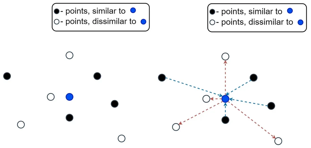
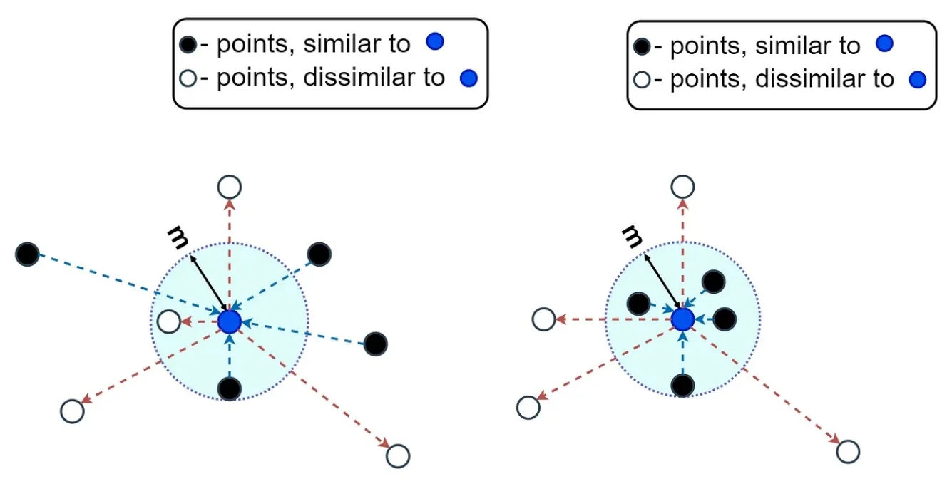
A Visual Summary of the Learning Objective The goal of contrastive learning is to shape the embedding space such that similar points are tightly clustered while dissimilar points are pushed away. This intuition is captured by minimizing the intra-class distances and maximizing the inter-class distances. Visually, we aim to shorten the intra-class arrows (from the anchor to similar samples) and lengthen the inter-class arrows (from the anchor to dissimilar samples).
Formally, for each anchor embedding \( \vec {z}_a \), we want: \[ \max _{i \in \mathcal {P}} \| \vec {z}_a - \vec {z}_i \|_2 < \min _{j \in \mathcal {N}} \| \vec {z}_a - \vec {z}_j \|_2, \] where \( \mathcal {P} \) denotes the set of similar (positive) examples and \( \mathcal {N} \) the set of dissimilar (negative) examples. This condition ensures that the most distant positive is still closer than the nearest negative—enabling accurate grouping under a simple nearest-neighbor decision rule.
This margin-based separation underpins the contrastive loss function introduced by Hadsell et al., which explicitly enforces that:
- Similar samples (label \( Y = 0 \)) fall within a small distance of the anchor;
- Dissimilar samples (label \( Y = 1 \)) are pushed outside a minimum margin \( m \).
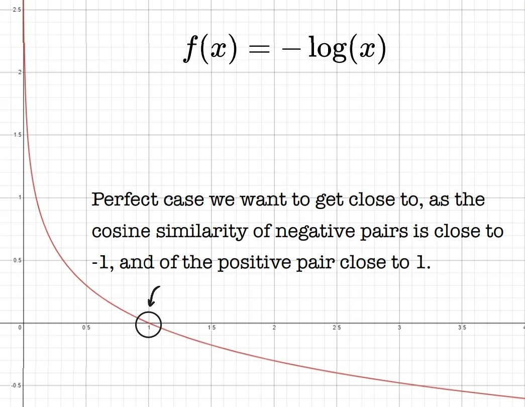
Why Not Use \( \frac {1}{D_W} \)? One might consider directly maximizing dissimilarity by minimizing \( \frac {1}{D_W} \), where \( D_W = \| G_{\boldsymbol {W}}(\vec {X}_1) - G_{\boldsymbol {W}}(\vec {X}_2) \|_2 \). However, such a formulation is unstable: the gradient of \( \frac {1}{D_W} \) diverges as \( D_W \to 0 \), which can lead to numerical instability and overfitting. Instead, Hadsell et al.’s formulation imposes a margin-based hinge on the dissimilar term: \[ \frac {1}{2} \left [ \max (0, m - D_W) \right ]^2, \] which saturates to zero once the dissimilar pair is sufficiently separated—yielding a more stable and robust learning signal.
From Supervision to Self-Supervision Originally developed for supervised settings with labeled pairs, contrastive loss has been adapted to the self-supervised regime by removing the need for manual annotations. In this formulation, positive pairs are created by applying two different augmentations to the same image, while negative pairs are defined implicitly by treating other images in the batch (or memory bank) as dissimilar.
This strategy enables scalable training on large unlabeled datasets while learning semantically meaningful embeddings. The underlying assumption is that different augmented views of the same image share the same semantic identity.
This idea forms the basis of prominent SSL methods such as SimCLR [89], which relies on large batches and strong augmentations, and MoCo [220], which uses a momentum encoder and memory bank to maintain negative examples across iterations.
These methods extend contrastive learning to instance-level discrimination tasks without labels, preserving the core objective: pull similar samples together and push dissimilar ones apart. We now illustrate how augmented views form anchor–positive–negative triplets used in contrastive training.
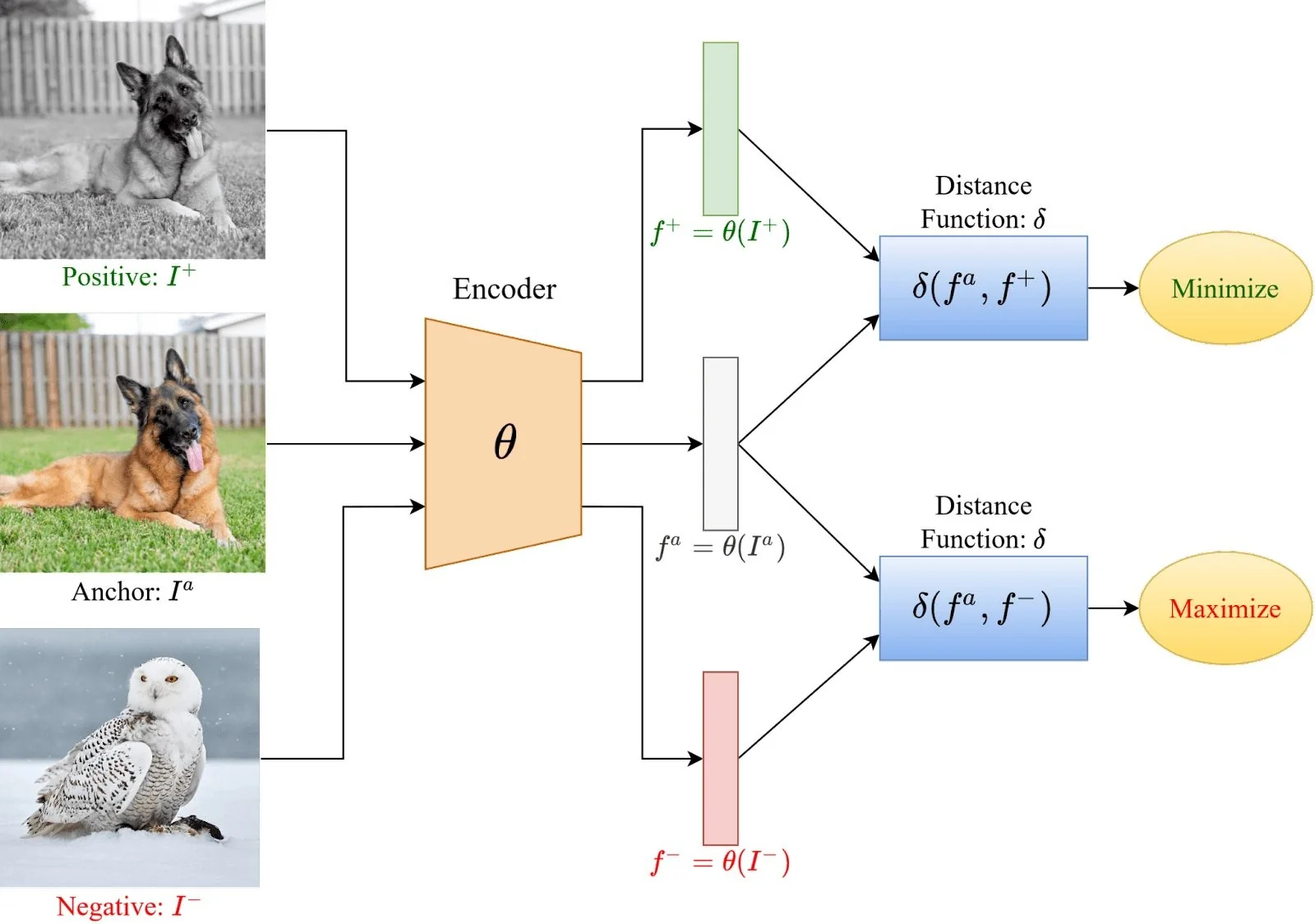
Triplet Setup: Anchor, Positive, Negative Every training batch uses:
- An anchor \( {I}^a \),
- A positive \( I^+ \), an augmented view of the anchor,
- Multiple negatives \( I^- \), views of different images.
The model learns to attract \( {I}^a \) and \( I^+ \), while repelling \( {I}^a \) from all \( I^- \).
This setting prepares the ground for more advanced losses like InfoNCE and NT-Xent, which we now derive.
22.3.3 The NT-Xent Loss: Normalized Temperature-Scaled Cross-Entropy
Overview and Purpose The NT-Xent loss (Normalized Temperature-Scaled Cross Entropy) was introduced in SimCLR [89] as a specialized instance of the broader InfoNCE loss. Its goal is to pull together embeddings of positive pairs—two different augmentations of the same image—while pushing apart negative pairs—augmentations of other images.
Unlike the more general InfoNCE, which allows a fixed number of negatives \(K\) (often stored in a memory bank), NT-Xent uses all other augmented samples within the batch as negatives. This batch-based construction, combined with cosine similarity and temperature scaling, makes NT-Xent self-contained, scalable, and well-suited for large-batch training without the need for external memory or momentum encoders.
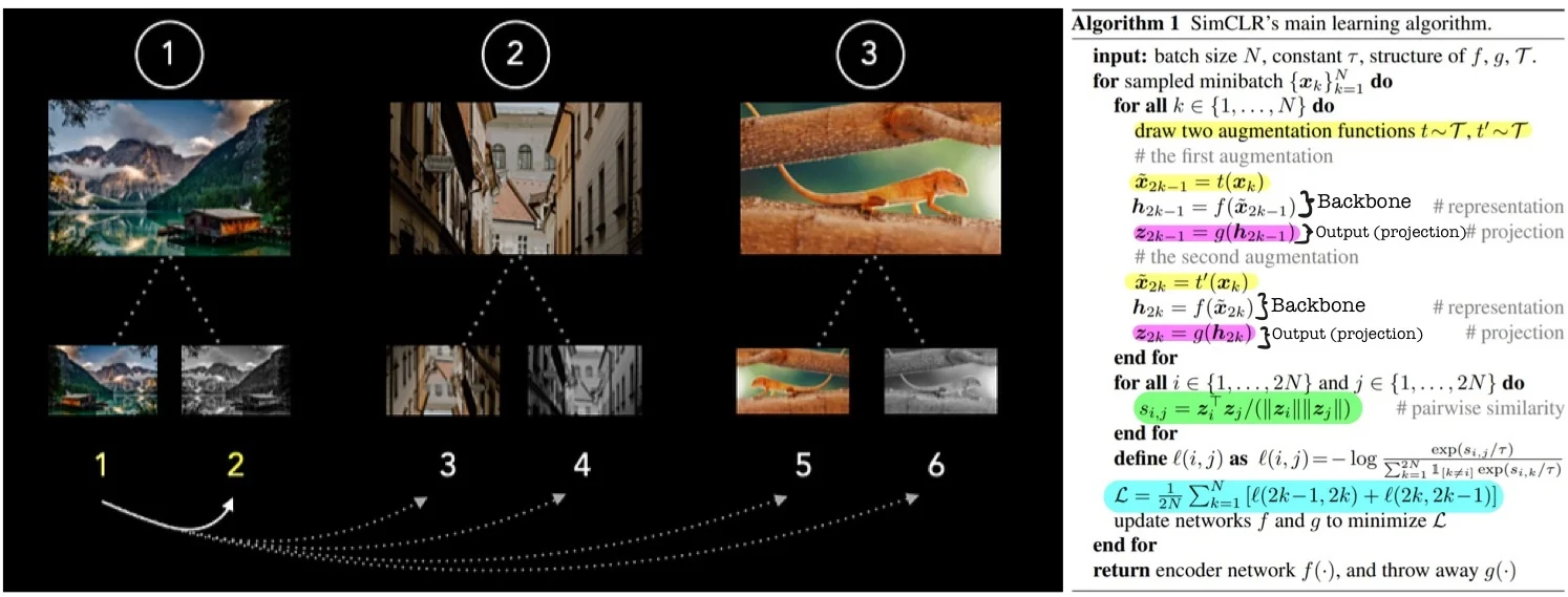
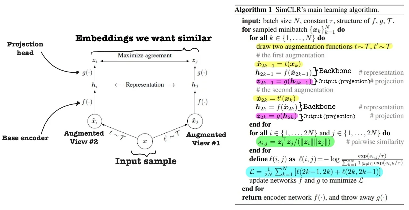
Pairwise Contrastive Loss: NT-Xent Formulation Given a batch of \( N \) training images, SimCLR applies two independent stochastic data augmentations to each, resulting in \( 2N \) views. These are passed through a shared encoder \( f(\cdot ) \) followed by a projection head \( g(\cdot ) \), producing representations \( \{ \mathbf {z}_1, \mathbf {z}_2, \dots , \mathbf {z}_{2N} \} \subset \mathbb {R}^d \). Each original image thus yields a positive pair: \( (\mathbf {z}_{2k-1}, \mathbf {z}_{2k}) \) for \( k = 1, \dots , N \).
Let \( \mathrm {sim}(\mathbf {z}_i, \mathbf {z}_j) \) denote the cosine similarity between embeddings \( \mathbf {z}_i \) and \( \mathbf {z}_j \), both normalized to unit length: \[ \mathrm {sim}(\mathbf {z}_i, \mathbf {z}_j) = \frac {\mathbf {z}_i^\top \mathbf {z}_j}{\|\mathbf {z}_i\| \cdot \|\mathbf {z}_j\|} \in [-1, 1]. \]
The NT-Xent loss for a positive pair \( (i, j) \) is defined as: \[ \ell (i, j) = -\log \frac {\exp \left (\mathrm {sim}(\mathbf {z}_i, \mathbf {z}_j)/\tau \right )}{\sum _{k=1}^{2N} \mathbb {1}_{[k \ne i]} \exp \left (\mathrm {sim}(\mathbf {z}_i, \mathbf {z}_k)/\tau \right )}, \] where \( \tau > 0 \) is a temperature hyperparameter that scales the logits in the softmax.
This loss encourages each anchor \( \mathbf {z}_i \) to be more similar to its corresponding positive \( \mathbf {z}_j \) than to any of the \( 2N - 2 \) remaining negatives in the batch. Importantly, the positive \( j \) is included in the denominator as part of the softmax normalization—framing the task as (soft) classification among all other examples, with the correct match being \( j \).
Batch Aggregation and the \( \frac {1}{2N} \) Factor Each of the \( 2N \) augmented views serves once as an anchor. Hence, the total batch loss averages over all \( 2N \) such anchor-positive loss terms: \[ \mathcal {L}_{\mbox{NT-Xent}} = \frac {1}{2N} \sum _{k=1}^{N} \left [ \ell (2k - 1, 2k) + \ell (2k, 2k - 1) \right ]. \]
The normalization factor \( \frac {1}{2N} \) ensures that the total loss is the mean over all anchor-based comparisons. Each sample contributes exactly one anchor-to-positive term (and is a target once for its positive), and the symmetry ensures both directions are treated equally.
The Role of Symmetry In SimCLR, each image gives rise to two independently augmented views, forming a positive pair. For each such pair \((i, j)\), the NT-Xent loss is computed twice: once treating \(i\) as the anchor and \(j\) as the positive, and once with roles reversed. This symmetric loss formulation is not redundant—it is a principled mechanism that enforces bidirectional learning and representational consistency.
A common misconception is that if the representation \(i\) is optimized to be similar to \(j\), then \(j\) will automatically become similar to \(i\). While this holds for the cosine similarity itself—since \(\mbox{sim}(z_i, z_j) = \mbox{sim}(z_j, z_i)\)—it does not hold for the gradients of the loss. The NT-Xent objective applies a softmax over all non-anchor embeddings for each anchor. Thus, in \(\ell (i, j)\), \(z_i\) is compared against all other examples to classify \(z_j\) as its match. In contrast, \(\ell (j, i)\) uses \(z_j\) as the anchor and normalizes over a different softmax distribution. Despite the symmetry of the similarity metric, the loss landscapes—and therefore the gradients—are different for \(\ell (i, j)\) and \(\ell (j, i)\). As a result, omitting either direction would lead to asymmetric learning and potentially degraded representations for one side of the pair.
- Balanced gradient updates: Each of the \(2N\) views in a batch acts as an anchor exactly once. This guarantees that every view receives a direct learning signal and contributes symmetrically to parameter updates.
- Reciprocal alignment: Symmetric loss ensures that both views learn to identify their counterpart among many negatives, encouraging mutual semantic agreement across augmentations.
- Gradient diversity and stability: By computing the loss in both directions, the batch yields twice as many anchor-positive training signals. This increased supervision reduces gradient variance and stabilizes convergence.
- Stronger collapse prevention: Symmetry amplifies the discriminative pressure by requiring every view to be uniquely identifiable from its counterpart. This discourages degenerate solutions where all embeddings collapse to the same point.
In summary, the symmetric NT-Xent loss is essential for learning robust, discriminative, and augmentation-invariant representations. It ensures that both views of each instance are held equally accountable during training, preventing one-sided learning and promoting mutual consistency across the feature space.
Illustration of the Loss Mechanism
Role of the Projection Head SimCLR applies the NT-Xent loss not on the encoder output \( h_i = f(\tilde {x}_i) \), but on a transformed embedding \( z_i = g(h_i) \) produced by a non-linear projection head \( g(\cdot ) \). This architectural choice serves multiple roles:
- Enhanced contrastive learning: The projection head maps features into a latent space tailored for the contrastive objective, often improving training efficiency and downstream alignment.
- Disentangled optimization: By separating the encoder and contrastive spaces, SimCLR allows \( f(\cdot ) \) to focus on learning transferable representations, while \( g(\cdot ) \) handles the invariance constraints of the contrastive task.
- Downstream effectiveness: Empirically, the encoder outputs \( h \) outperform the projected representations \( z \) on downstream tasks. This suggests that \( g(\cdot ) \) discards non-semantic variation useful only during pretraining—preserving generality in \( f(\cdot ) \).
For each positive pair, we want the similarity score \( s_{i,j} \) to dominate the softmax numerator, while all other similarity scores are minimized in the denominator. This aligns positive pairs and repels negative ones in angular space.
Summary NT-Xent effectively replaces the contrastive margin in Hadsell’s formulation with a temperature-scaled softmax. It eliminates the need for threshold tuning, is differentiable everywhere, and naturally fits into batch-wise contrastive pipelines.
We now examine two key contrastive frameworks: SimCLR, which uses NT-Xent with large in-batch negatives, and MoCo, which introduces a momentum encoder and memory queue for scalable contrastive learning. We start with SimCLR, then follow MoCo through its three versions.
22.3.4 SimCLR: A Simple Framework for Contrastive Learning
Overview SimCLR [89] introduced a surprisingly simple yet powerful framework for self-supervised contrastive learning that achieved state-of-the-art performance using standard architectures and without requiring negative mining tricks or memory banks. Its core training objective is the NT-Xent loss, introduced in part 22.3.3, which pulls together positive pairs while pushing apart negatives in the embedding space.
Architecture Components The SimCLR framework is composed of the following components:
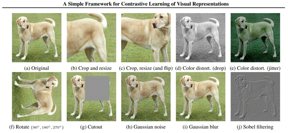
- Stochastic Data Augmentation Module: Each image is transformed into two augmented views using strong random transformations (e.g., random cropping, color distortion, blur), forming a positive pair. Other images in the batch form negative pairs.
- Encoder Network \( f(\cdot ) \): A standard ResNet (e.g., ResNet-50) extracts a representation vector \( {h} \in \mathbb {R}^d \) from each augmented view.
- Projection Head \( g(\cdot ) \): A small MLP maps \( {h} \) to a lower-dimensional vector \( {z} = g({h}) \), on which the contrastive loss is applied.
The paper’s critical finding is that while contrastive training is applied to \( {z} \), the upstream encoder output \( {h} \) consistently yields better performance on downstream tasks. The projection head thus acts as a form of task-specific decoupling, allowing the encoder to retain general-purpose semantics while contrastive alignment occurs in \( {z} \)-space.
Design Principles Behind SimCLR Beyond its loss function, SimCLR’s success hinges on several essential design insights:
- Strong Data Augmentations Are Crucial: SimCLR demonstrated empirically that augmentations such as random crop, color distortion, and Gaussian blur are not mere regularizers but define the pretext task by creating diverse views of the same image.
- Importance of the Projection Head: Removing the non-linear head or applying the contrastive loss directly on \( {h} \) significantly degraded performance. This architectural separation was essential for avoiding information loss and achieving strong transferability.
- Large Batch Sizes: NT-Xent is computed over all other \( 2N-2 \) samples as negatives. Larger batches improve the quality of negative sampling, and SimCLR scaled up to batch sizes of 8192 using 128 TPU cores.
- Temperature Scaling: The temperature parameter \( \tau \) controls the sharpness of the similarity distribution and strongly affects performance. Lower values increase contrastiveness but can destabilize training; careful tuning is needed.
Training Configuration and Stability SimCLR’s strong performance was not only due to its contrastive loss and data augmentations, but also to its rigorous training setup. The model was trained for 1000 epochs—an unusually long schedule—using large batch sizes of up to 8192.
These batch sizes are essential for generating a sufficient number of negative examples within each batch (e.g., 16,382 negatives per positive pair at batch size 8192). To enable stable optimization under such conditions, SimCLR used the LARS optimizer [761], which supports large-batch training with high learning rates.
The learning rate followed a linear warm-up for the first 10 epochs, followed by a cosine decay schedule without restarts. Training also relied heavily on strong data augmentations, including color distortions, random cropping, and Gaussian blur, which proved more impactful for contrastive learning than for supervised settings. Despite its conceptual simplicity, SimCLR was computationally intensive: a full 1000-epoch training of ResNet-50 required multiple days on TPU pods or dozens of V100 GPUs.
Performance Benchmarks SimCLR established new benchmarks for self-supervised learning:
- Linear evaluation protocol: When training a linear classifier atop frozen features, SimCLR achieved 76.5% top-1 accuracy on ImageNet with a ResNet-50 encoder—on par with fully supervised ResNet-50 models. This confirmed that self-supervised pretraining could match label-based training in representation quality.
- Label efficiency: In semi-supervised settings, SimCLR dramatically outperformed supervised baselines. Fine-tuning on just 1% of ImageNet labels yielded substantially better accuracy than supervised models trained on the same data subset. This demonstrates the method’s exceptional ability to learn from scarce annotations.
- Transferability: SimCLR’s representations transferred effectively to downstream tasks beyond ImageNet. Across 12 natural image classification datasets, SimCLR matched or surpassed a supervised ResNet-50 baseline on 10 of them, demonstrating robustness and generality.
These results highlight that scaling contrastive learning—through larger batches, longer training, and effective augmentations—can yield powerful representations without the need for human labels, and can generalize across domains.
Visualization of SimCLR Pipeline
Limitations and the Road to MoCo Despite its success, SimCLR suffers from a key limitation: its reliance on extremely large batch sizes. Since all negatives are sampled in-batch, sufficient diversity requires thousands of negatives per anchor—demanding massive compute. This constraint motivates subsequent approaches such as MoCo, which replace batch-based negatives with a dynamic memory bank and a momentum encoder, offering comparable performance with smaller batches.
We now turn to MoCo [220], a method that addresses this limitation by introducing a scalable and memory-efficient alternative to batch-based contrastive learning.
22.3.5 Momentum Contrast (MoCo)
Motivation: Avoiding Large Batch Sizes SimCLR demonstrated that contrastive learning benefits significantly from large numbers of negative examples. However, it used in-batch negatives only, meaning the number of negatives was tied to the batch size. To provide over 8000 negatives per anchor (as in SimCLR), one must train with prohibitively large batches—e.g., 8192 samples—across dozens of GPUs with high memory budgets.
MoCo [220] was introduced to overcome this scalability bottleneck. Its core idea is to decouple the number of negatives from the batch size by maintaining a large, dynamic dictionary (queue) of past embeddings. It also introduces a momentum encoder to ensure that the representations stored in this queue evolve slowly and remain consistent over time—enabling effective contrastive learning with a small batch and many stable negatives (previously stored in a FIFO queue).
Core Architecture MoCo adopts an asymmetric dual-encoder architecture, consisting of:
- Query encoder \( f_q \): a standard neural network (e.g., ResNet-50) trained via backpropagation.
- Key encoder \( f_k \): a second encoder with the same architecture, whose parameters are updated as a moving average of \( f_q \): \[ \theta _k \leftarrow m \cdot \theta _k + (1 - m) \cdot \theta _q \] This momentum update with \( m \approx 0.999 \) ensures that \( f_k \) evolves slowly, producing temporally consistent keys that can be stored in a queue and reused as negatives across multiple steps.
Terminology note. MoCo replaces the classical anchor–positive–negative triplet terminology with the more functional terms query (trainable view) and key (reference views). The positive key comes from the same image as the query, while negatives are sampled from the memory queue.
Contrastive Loss in MoCo MoCo adopts the InfoNCE loss, mathematically identical to the NT-Xent loss in SimCLR. For a query \( q = f_q(x_q) \), a positive key \( k^+ = f_k(x_k^+) \), and a set of negatives \( \{ k_i^- \} \) drawn from the queue \( \mathcal {K} \), the loss is: \[ \mathcal {L}_{\mbox{MoCo}} = -\log \frac {\exp (q \cdot k^+ / \tau )}{\exp (q \cdot k^+ / \tau ) + \sum _{k^- \in \mathcal {K}} \exp (q \cdot k^- / \tau )} \] The query and its positive key are two augmentations of the same image, while the negatives come from different images (past embeddings stored in the queue).
MoCo Training Pipeline Each training step proceeds as follows:
- 1.
- Sample a batch of images; for each image, create two augmentations: \( x_q \) and \( x_k \).
- 2.
- Pass \( x_q \) through the query encoder \( f_q \) to produce the query \( q \).
- 3.
- Pass \( x_k \) through the key encoder \( f_k \) to obtain the key \( k^+ \). No gradients flow through \( f_k \).
- 4.
- Compute the InfoNCE loss between \( q \), \( k^+ \), and negatives \( \{ k^- \} \) in the queue.
- 5.
- Backpropagate gradients to update \( f_q \).
- 6.
- Update \( f_k \) using exponential moving average (EMA) of \( f_q \).
- 7.
- Enqueue the new key \( k^+ \) and dequeue the oldest key to maintain queue size.
Why MoCo Works: Scale, Stability, and Efficiency MoCo addresses two core challenges in contrastive learning: the need for many negatives and the requirement for stable targets. Its architecture offers a scalable and hardware-efficient alternative to large-batch contrastive methods like SimCLR.
- Large-scale negatives without large batches: In SimCLR, negatives are limited to samples within the current batch, requiring extremely large batch sizes (e.g., 8192) to match the number of negatives MoCo can access. MoCo overcomes this limitation through a dynamic queue: a FIFO buffer of encoded key representations from prior mini-batches. This decouples the number of negatives from the current batch size, allowing MoCo to leverage tens of thousands of negatives per step (e.g., a queue of 65,536) while training with batches as small as 256—greatly reducing the compute and memory burden.
- Stable representations through momentum: To ensure that the queue remains semantically consistent with the current encoder, MoCo employs a momentum encoder. The key encoder \( f_k \) is updated as an exponential moving average (EMA) of the query encoder \( f_q \): \[ \theta _k \leftarrow m \cdot \theta _k + (1 - m) \cdot \theta _q \] A high momentum (e.g., \( m = 0.999 \)) ensures that \( f_k \) evolves slowly across training steps. This stabilizes the embeddings stored in the queue and prevents contrastive comparisons from drifting out of alignment. Without this slow evolution, earlier keys would quickly become obsolete, leading to noisy or contradictory learning signals.
- Asymmetric training improves robustness: Only the query encoder \( f_q \) is trained with gradients, while the key encoder \( f_k \) passively tracks it via momentum. This architectural asymmetry improves training stability, reduces memory requirements, and avoids collapse. By decoupling the learning dynamics of the two encoders, MoCo implicitly regularizes the training objective, making the contrastive task more stable and better behaved.
What the Queue Enables Unlike SimCLR, which must compute all negatives on-the-fly within the current batch, MoCo separates negative storage from computation. This leads to multiple advantages:
-
Extremely large dictionaries: MoCo’s queue holds thousands of negatives—potentially 100× more than what can fit in a single batch. This increases the diversity of the contrastive signal and improves the model’s ability to discriminate among fine-grained features in high-dimensional space.
- Efficient memory and compute: Only the current batch is encoded by \( f_q \) and \( f_k \), while prior embeddings are reused from the queue without recomputation. This constant per-step cost enables MoCo to scale up the effective batch size without scaling GPU memory usage.
- Temporal coherence: The queue is updated at each step by enqueuing newly encoded positive keys and removing the oldest entries. Because the key encoder evolves slowly via EMA, even old entries in the queue remain consistent with the current representation space. Without this, the contrastive task would break down—indeed, MoCo fails to train when \( m = 0 \).

Momentum Hyperparameter Tuning and Ablation Results A central component of MoCo’s architecture is the momentum-based update of the key encoder \( f_k \), governed by an exponential moving average (EMA):
\[ \theta _k \leftarrow m \cdot \theta _k + (1 - m) \cdot \theta _q \]
Here, \( \theta _q \) and \( \theta _k \) denote the parameters of the query and key encoders, respectively, and \( m \in [0, 1) \) is the momentum coefficient.
This update rule ensures that the representations stored in the queue—many of which were computed several iterations earlier—remain temporally consistent with the current query space. A high momentum slows the evolution of \( f_k \), thereby maintaining coherence among the stored negatives. In contrast, a low momentum causes \( f_k \) to change rapidly, making the queue misaligned with the current query distribution and impairing training.
| \( m \) | 0 | 0.9 | 0.99 | 0.999 | 0.9999 |
| Accuracy (%) | fail | 55.2 | 57.8 | 59.0 | 58.9 |
As shown in Table 22.2, the model’s performance is highly sensitive to the value of \( m \). When \( m = 0 \), MoCo fails entirely—the key encoder becomes a direct copy of the query encoder, causing the queue to drift erratically and undermining consistency. At the other extreme, very high momentum values (e.g., \( m = 0.999 \)) yield the best performance by preserving alignment across steps while still allowing the queue to adapt gradually. These findings emphasize that consistency is more important than freshness in maintaining a reliable dictionary for contrastive learning.
Other Key Ablations and Design Justifications In addition to momentum tuning, the MoCo v1 paper includes several important ablations that support its architectural decisions:
- Queue size \( K \): Larger queues consistently improve performance. Increasing \( K \) from 4,096 to 65,536 enables access to more diverse negatives without great additional computational cost, as only the current mini-batch is encoded.
-
Contrastive loss mechanisms: MoCo is compared to two alternatives: (i) a memory bank that stores outdated keys, and (ii) an end-to-end encoder that uses in-batch negatives. All mechanisms benefit from larger negative sets, but MoCo outperforms the others by maintaining both scale and temporal consistency.
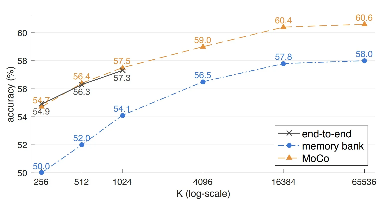
Figure 22.12: Comparison of three contrastive loss mechanisms on the ImageNet linear classification benchmark using a ResNet-50 backbone. All models share the same pretext task and differ only in their contrastive design. The number of negatives is \( K \) for MoCo and memory bank methods, and \( K - 1 \) for end-to-end approaches (excluding the positive sample). MoCo matches or surpasses the accuracy of both alternatives by combining a large pool of negatives with temporally consistent embeddings—achieving strong performance without relying on massive batches or tolerating stale keys. Source: [220]. -
Shuffling BatchNorm: In distributed training, naive use of Batch Normalization (BN) can introduce information leakage between the query and key branches. Since BN computes statistics across a batch, both the query and its corresponding positive key—if processed within the same synchronized batch—may indirectly share feature information through shared normalization. This enables the model to ”cheat” the pretext task by manipulating BN statistics, resulting in artificially low loss without truly learning semantic structure.
To mitigate this, MoCo applies batch shuffling for the key encoder: samples are randomly permuted before being distributed across GPUs. As a result, the BN statistics used in the query and key branches are computed over different sample subsets. This decouples their normalization pathways and forces the model to solve the contrastive task based on actual feature alignment rather than statistical shortcuts. Ablation results show that disabling this trick leads to significant performance degradation, underscoring its role in enabling genuine contrastive learning.
- Transfer performance: MoCo’s learned representations generalize well to downstream tasks. When fine-tuned on PASCAL VOC, COCO detection, or keypoint estimation, MoCo-pretrained models often outperform supervised counterparts, especially under low-data regimes.
Together, these results establish MoCo as a scalable and principled solution to the limitations of in-batch contrastive methods. Its success laid the groundwork for subsequent improvements in MoCo v2 and MoCo v3.
Performance and Comparison with SimCLR MoCo achieves comparable results (though lesser in this version) to SimCLR with dramatically lower resource demands:
| Aspect | SimCLR | MoCo |
|---|---|---|
| Negatives Source | In-batch only | External memory queue |
| Batch Size Requirement | Very large (up to 8192) | Small/moderate (e.g., 256) |
| Architectural Symmetry | Symmetric (same encoder) | Asymmetric (EMA target) |
| Update Mechanism | SGD on both encoders | SGD + EMA |
| Memory Usage | High (due to batch size) | Efficient |
| Collapse Prevention | Large batch + symmetry | Stable queue + EMA encoder |
From MoCo v1 to MoCo v2 MoCo v1 successfully decoupled negative sampling from batch size, enabling scalable contrastive learning with modest compute. However, its initial formulation was deliberately minimal—focused on demonstrating feasibility rather than achieving state-of-the-art accuracy. This left room for improvement. MoCo v2 [96] builds directly on the core architecture of MoCo v1 but integrates empirical best practices from SimCLR, including stronger data augmentations, a deeper nonlinear projection head, and cosine learning rate decay. These enhancements are orthogonal to the momentum-queue mechanism and can be applied without changing MoCo’s fundamental contrastive structure. As a result, MoCo v2 significantly boosts linear evaluation performance, closing the gap with—and in some settings surpassing—SimCLR, all while maintaining the efficiency and stability of the original framework.
22.3.6 MoCo v2 and MoCo v3
From MoCo v1 to v2: Architectural Refinements Following the success of MoCo [220], the second version—MoCo v2 [96]—introduced two impactful modifications inspired by SimCLR [89]:
- Replacing the ResNet encoder’s linear head with a 2-layer MLP projection head (2048-d hidden layer, ReLU nonlinearity).
- Augmenting the training pipeline with stronger augmentations, specifically adding Gaussian blur.
While these changes appear minor, they yield significant accuracy gains during unsupervised training. Notably, MoCo v2 maintains MoCo v1’s core design: a dynamic queue of negative keys and a momentum encoder. These enhancements allow MoCo v2 to surpass SimCLR in performance—despite requiring significantly smaller batch sizes.
MLP Head and Temperature Ablation. The following table—based on results from [96]—highlights the influence of the MLP projection head and temperature parameter \( \tau \) on ImageNet linear classification accuracy:
| \(\tau \) | 0.07 | 0.1 | 0.2 | 0.3 | 0.4 | 0.5 |
|---|---|---|---|---|---|---|
| w/o MLP | 60.6 | 60.7 | 59.0 | 58.2 | 57.2 | 56.4 |
| w/ MLP | 62.9 | 64.9 | 66.2 | 65.7 | 65.0 | 64.3 |
Comparison with SimCLR. As further demonstrated in Table 22.5, MoCo v2 [96] achieves competitive or superior performance compared to SimCLR, despite using significantly smaller batch sizes and fewer computational resources.
MoCo v3: Adapting Momentum Contrast to Vision Transformers With the rise of Vision Transformers (ViTs) [134], MoCo v3 [94] extended the momentum contrastive learning framework beyond convolutional backbones. It introduces several architectural and algorithmic updates that make it well-suited for training Transformer-based encoders in a scalable, stable, and contrastive manner.
Key innovations of MoCo v3 include:
- Removal of the memory queue: Unlike MoCo v1 and v2, MoCo v3 discards the dictionary queue and adopts an in-batch negatives strategy like SimCLR. This is made viable by scaling up batch sizes (e.g., 2048–4096), ensuring sufficient negative diversity without external memory.
- Symmetric contrastive loss: Previous versions used an asymmetric loss—queries were trained to match fixed keys. In MoCo v3, both augmented views are treated symmetrically: the loss is computed as \( \mathcal {L}(q_1, k_2) + \mathcal {L}(q_2, k_1) \), leveraging the full batch and encouraging bi-directional alignment.
- Non-shared prediction head: A learnable prediction MLP is appended only to the query encoder \( f_q \). This design, borrowed from BYOL, avoids trivial alignment and improves training stability by introducing asymmetry between encoders.
-
Frozen random patch projection in ViTs: MoCo v3 introduces a seemingly counter-intuitive yet effective design: when using ViTs, the patch projection layer—which maps image patches into token embeddings—is randomly initialized and then frozen. This layer is not trained; instead, a stop-gradient operator is applied immediately after it. The rationale stems from a key observation: during self-supervised ViT training, sharp gradient spikes frequently originate in the shallowest layers, particularly the patch projection. These spikes cause unstable optimization and mild accuracy degradation (e.g., 1–3%). Freezing this projection layer eliminates this instability, yielding smoother loss curves and higher final accuracy.
Importantly, the frozen projection still preserves input information due to the overcomplete nature of the embedding (e.g., mapping from 768 raw pixels to a 768-dimensional vector), making random projection surprisingly effective. While it may seem preferable to use a pretrained patch embedder, doing so would violate the self-supervised training regime’s independence from labeled data. The frozen random projector thus offers a principled compromise: it avoids instability without introducing supervision or sacrificing downstream performance.
These architectural innovations result in a streamlined and highly effective self-supervised training procedure. The following pseudocode illustrates the core training loop of MoCo v3 in PyTorch-like syntax, highlighting the interplay between query and key encoders, augmentation symmetry, and momentum updates:
# f_q: backbone + projection MLP + prediction MLP
# f_k: backbone + projection MLP (momentum-updated)
# m: momentum coefficient
# t: temperature

for x in loader:                   # Load a minibatch of N samples
    x1, x2 = aug(x), aug(x)        # Two random augmentations per sample

    q1, q2 = f_q(x1), f_q(x2)      # Query embeddings (with pred head)
    k1, k2 = f_k(x1), f_k(x2)      # Key embeddings (no pred head)

    loss = ctr(q1, k2) + ctr(q2, k1)   # Symmetric InfoNCE loss
    loss.backward()

    update(f_q)                    # SGD update for query encoder
    f_k = m * f_k + (1 - m) * f_q  # EMA update for key encoder
Loss Function. MoCo v3 uses a symmetric InfoNCE loss computed over in-batch negatives. Each query is matched to its corresponding key, and all other entries in the batch act as negatives:
def ctr(q, k):
    logits = mm(q, k.t())    # NxN cosine similarities
    labels = range(N)            # Positive pairs on the diagonal
    loss = CrossEntropyLoss(logits/t, labels)
    return 2 * t * loss           # Scaling to match SimCLR convention
This formulation treats each pair \( (q_i, k_i) \) as positive, and the remaining \( N - 1 \) entries in each row as negatives. The temperature \( t \) adjusts the sharpness of the distribution, and the scaling factor \( 2t \) compensates for the bidirectional loss.
Why Symmetric Loss? Earlier MoCo variants used an asymmetric loss because they relied on an external queue whose keys were not mutually comparable. MoCo v3, by operating on synchronized in-batch keys, can safely match both \( q_1 \rightarrow k_2 \) and \( q_2 \rightarrow k_1 \). This symmetry increases gradient diversity, ensures both views act as anchors, and improves the robustness of learned representations.
- The query encoder \( f_q \) is updated via SGD and includes both a projection and prediction head.
- The key encoder \( f_k \) is updated via exponential moving average (EMA) of \( f_q \), and has no prediction head.
- The contrastive loss uses all \( N - 1 \) in-batch samples as negatives for each query.
- Symmetric training ensures both augmented views serve equally as anchor and target, avoiding representational bias.
Performance Highlights MoCo v3 achieves state-of-the-art results on ImageNet using both CNN and ViT backbones. Tables 22.6 and 22.7 show MoCo v3 outperforming or matching alternatives like BYOL and SimCLR across multiple settings.
| Backbone | ViT-B | ViT-L | ViT-H |
| Linear Probing | 76.7 | 77.6 | 78.1 |
| End-to-End Finetuning | 83.2 | 84.1 | – |
Takeaway MoCo v3 elegantly unifies contrastive learning with Transformer architectures by (1) removing the queue, (2) adopting a symmetric InfoNCE loss, and (3) introducing practical stability mechanisms like frozen embeddings and non-shared heads. These changes not only boost performance but also simplify training and broaden applicability across vision architectures.
22.3.7 SimCLR v2: Scaling Contrastive Learning for Semi-Supervised Settings
Motivation and Overview SimCLR v1 [89] showed that strong visual representations can be learned without labels by leveraging contrastive learning with the NT-Xent loss (see 22.3.3). However, its focus was limited to unsupervised pretraining with moderate architectures and did not provide a full pipeline for label-efficient learning. To address this, SimCLR v2 [90] introduces a scalable and modular framework that unifies contrastive pretraining, supervised fine-tuning, and self-distillation. The result is a general-purpose pipeline for semi-supervised learning that achieved (at the time of publication) state-of-the-art performance in low-label regimes, while also improving linear evaluation and transfer capabilities.
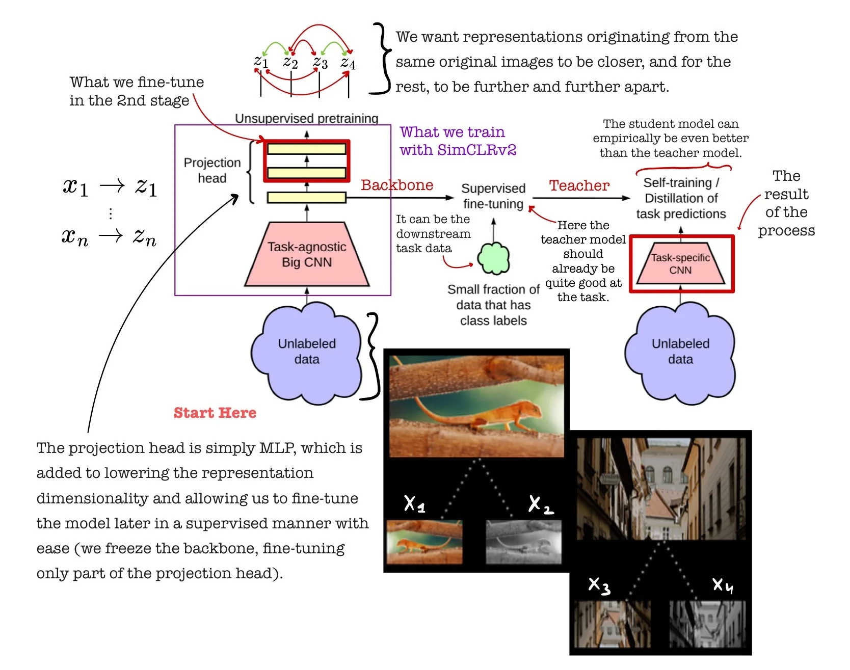
Three-Stage Training Framework SimCLR v2 introduces a structured pipeline that combines large-scale self-supervised pretraining, label-efficient supervised fine-tuning, and knowledge distillation. This enables strong performance in both self- and semi-supervised regimes by leveraging unlabeled data at scale and making effective use of limited labels.
- 1.
- Unsupervised Pretraining: A high-capacity encoder (e.g., ResNet-152 or ResNet-152+SK) is trained using the SimCLR contrastive objective on large-scale unlabeled data. This stage learns augmentation-invariant features by bringing together representations of the same image under different views while repelling those from different images. Larger encoders capture more diverse semantic structure, aiding downstream generalization.
- 2.
- Supervised Fine-tuning: The pretrained encoder is fine-tuned on a small labeled subset (e.g., 1–10% of ImageNet). Rather than discarding the projection head, fine-tuning starts from an intermediate layer (layer_2) of the MLP, preserving useful invariances and improving performance under low-label settings.
- 3.
- Knowledge Distillation: The fine-tuned model acts as a teacher for a student network, which is trained on unlabeled data using soft labels (logits or probabilities). These soft targets encode inter-class structure and uncertainty, guiding the student to learn smoother and more generalizable decision boundaries. Surprisingly, the student can even outperform the teacher.
Architectural Enhancements and Ablation Insights SimCLR v2 enhances SimCLR v1 through several key refinements:
- Larger Encoders: Using deeper and wider networks, such as ResNet-152+SK, improves representation quality learned from unlabeled data.
- Three-Layer Projection Head: The projection MLP \( g(\cdot ) \), extended from 2 to 3 layers, \[ z = W_3 \cdot \mbox{ReLU}(W_2 \cdot \mbox{ReLU}(W_1 h)), \] increases the head’s expressiveness for contrastive learning while decoupling it from the encoder \( f(\cdot ) \), which remains focused on learning transferable features.
- Mid-layer Fine-tuning: Fine-tuning from the second hidden layer of \( g(\cdot ) \) bridges pretraining and downstream tasks, acting as a task-adaptive adapter and improving label efficiency.
Why Distillation Works The distillation step enables the student to benefit from the teacher’s knowledge—even exceeding it—through several mechanisms:
- Soft Targets as Rich Supervision: Unlike hard labels, soft labels encode class similarities and model uncertainty, offering a smoother and more informative learning signal.
- Regularization via Teacher Guidance: The teacher’s outputs act as denoised supervision, reducing overfitting to limited labels and improving generalization.
- Expanded Supervision from Unlabeled Data: By assigning soft labels to the entire unlabeled set, the student trains on a vastly expanded pseudo-labeled dataset.
- Simpler Optimization Objective: Mimicking the teacher’s output distribution is often easier than learning the task from scratch with limited labels, enabling more stable and efficient training.
- Student Surpassing Teacher: The student can outperform its teacher because it trains on more data (via distillation) with richer supervision, while regularized by the teacher’s knowledge.
Quantitative Results and Analysis To assess SimCLR v2’s performance under semi-supervised conditions, the authors evaluate its accuracy on ImageNet using 1% and 10% of labels. Following a two-stage protocol—self-supervised pretraining followed by supervised fine-tuning and distillation—SimCLR v2 achieves substantial improvements over both prior self-supervised methods and strong semi-supervised baselines. The table below reports Top-1 and Top-5 accuracy using various ResNet architectures and training setups.
| Method | Architecture | 1% T1 | 1% T5 | 10% T1 | 10% T5 |
|---|---|---|---|---|---|
| Supervised baseline [90] | ResNet-50 | 25.4 | 48.4 | 56.4 | 80.4 |
| SimCLR v1 [89] | R-50 (4\(\times \)) | 63.0 | 85.8 | 74.4 | 92.6 |
| BYOL [194] | R-200 (2\(\times \)) | 71.2 | 89.5 | 77.7 | 93.7 |
| SimCLR v2 (distilled) | R-50 | 73.9 | 91.5 | 77.5 | 93.4 |
| SimCLR v2 (distilled) | R-50 (2\(\times \)+SK) | 75.9 | 93.0 | 80.2 | 95.0 |
| SimCLR v2 (self-distilled) | R-152 (3\(\times \)+SK) | 76.6 | 93.4 | 80.9 | 95.5 |
Table 22.8 shows that with just 1% of labels (approximately 13 images per class), SimCLR v2 with ResNet-152 (3\(\times \) wider + SK convolutions) achieves 76.6% Top-1 accuracy and 93.4% Top-5 accuracy, outperforming all prior methods.
| Training Setup | 1% Labels | 10% Labels |
|---|---|---|
| Label only | 12.3 | 52.0 |
| Label + distill (labeled only) | 23.6 | 66.2 |
| Label + distill (labeled + unlabeled) | 69.0 | 75.1 |
| Distill only (unlabeled only) | 68.9 | 74.3 |
Table 22.9 presents ablations on distillation strategy. Notably, a comparable performance to the best one is achieved even without any labeled examples during the distillation phase. This demonstrates the strength of soft-label supervision: learning from the teacher’s logits—even on fully unlabeled data—transfers robust knowledge.
Table 22.10 reports linear evaluation accuracy for ResNet-50 (1\(\times \)) backbones. SimCLR v2 substantially improves over SimCLR v1 and MoCo v2, nearly matching the fully supervised model despite using no labels during pretraining.
Conclusion The SimCLR family demonstrates the power of contrastive learning to scale with model capacity and data availability. Starting from its first version [89], which emphasized instance discrimination with large batch sizes and strong augmentations, SimCLR v2 [90] extended this foundation into a full semi-supervised framework. It combines:
- Stronger encoders and augmentations during large-scale contrastive pretraining,
- A deeper projection head with mid-layer fine-tuning to retain invariant features,
- Soft-label distillation to extract value from unlabeled data—even without further label supervision.
These advances allow SimCLR v2 to achieve top-tier performance across both low-label and fully supervised regimes. However, while effective, SimCLR remains a purely instance-level learner, optimizing contrast between individual examples rather than trying to capture the semantic structure of the data manifold directly.
This motivates the next family of methods—ReLIC (REpresentation Learning via Invariant Causal mechanisms)—which extends contrastive learning by incorporating relational and group-level constraints, paving the way for more robust and causally grounded representations.
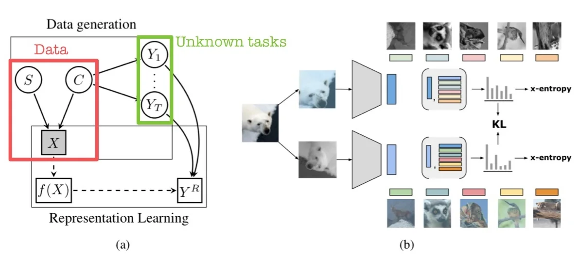
22.3.8 ReLIC: Representation Learning via Invariant Causal Mechanisms
Motivation and Causal Assumptions ReLIC [450] introduces a causal lens to self-supervised representation learning by explicitly aiming to disentangle content from style. The method assumes that each observed image \( X \) is generated by two independent latent factors: \[ X = g(C, S) \] where:
- \( C \) denotes the content—the semantically relevant signal such as object identity, shape, or structure.
- \( S \) represents the style—the nuisance variation such as color, lighting, texture, or viewpoint.
and assumes statistical independence between them: \( C \perp S \). This separation echoes the intuition that the identity of an object (e.g., “cat”) does not depend on superficial visual properties like background or illumination.
To formalize its invariance objective, ReLIC relies on the causal do-calculus [491]. Specifically, for any downstream task \( Y_t \), the model assumes that predictions should be based solely on content \( C \), and remain unchanged under interventions on style \( S \). This is written as: \[ p^{\mathrm {do}(S = s_i)}(Y_t \mid C) = p^{\mathrm {do}(S = s_j)}(Y_t \mid C), \quad \forall s_i, s_j \in \mathcal {S} \] Here, \( p^{\mathrm {do}(S = s)}(Y_t \mid C) \) denotes the interventional distribution—the probability of label \( Y_t \) conditioned on content \( C \), under a hypothetical external intervention that forces the style variable \( S \) to take the value \( s \). The use of do-notation, introduced by Pearl, distinguishes causal effects from observational correlations. In this context, it encodes the notion that the label of an image (e.g., “zebra”) should not change merely because the background shifts from grassland to water, or the lighting changes from day to dusk.
Example: Consider two augmentations of an image of a red car—one where the car appears under daylight and one under shadows. While these views differ in pixel space, the object’s identity is the same. A causally robust model should therefore map both views to the same semantic representation, ignoring the nuisance introduced by style.
In ReLIC, such interventions on \( S \) are simulated using common data augmentations (e.g., random crop, color jitter, Gaussian blur), and the goal becomes to learn a representation \( f(X) \) that reflects \( C \) while being invariant to such augmentations. By explicitly encouraging prediction consistency across different styles, ReLIC aligns representation learning with the causal invariance principle: semantic meaning should remain stable under changes that do not alter the underlying content.
Learning via Invariant Proxy Prediction Since the latent variables \( C \), \( S \), and \( Y_t \) are unobserved during training, ReLIC introduces a self-supervised proxy objective that indirectly enforces the causal invariance principle. Specifically, it defines:
- A proxy task \( Y^R \), instantiated as instance discrimination—distinguishing each image from all others.
- A set of augmentations \( \mathcal {A} = \{a_1, a_2, \dots \} \) that preserve content but vary style. These are treated as interventions on the style variable \( S \).
- A learned encoder \( f(X) \), which is optimized to approximate the latent content variable \( C \).
The central learning principle is that predictions of the proxy task should remain invariant under different style interventions: \[ p^{\mathrm {do}(a_i)}(Y^R \mid f(X)) = p^{\mathrm {do}(a_j)}(Y^R \mid f(X)), \quad \forall a_i, a_j \in \mathcal {A} \] This means that although the augmentations \( a_i, a_j \) may alter stylistic attributes (e.g., color, background), the identity prediction of the image via the proxy task \( Y^R \) should remain unchanged when computed on the representation \( f(X) \).
To implement this, ReLIC defines a joint loss consisting of two components:
- 1.
- A standard contrastive loss (e.g., InfoNCE) that encourages positive pairs to be close and negative pairs to be apart.
- 2.
- An explicit invariance penalty, formalized as a Kullback–Leibler (KL) divergence between the predicted proxy distributions across different augmentations: \[ \mathcal {L}_{\mathrm {inv}} = D_{\mathrm {KL}} \left ( p(Y^R \mid f(a_i(X))) \parallel p(Y^R \mid f(a_j(X))) \right ) \]
The full ReLIC objective is a weighted sum of these terms: \[ \mathcal {L}_{\mathrm {ReLIC}} = \mathcal {L}_{\mathrm {contrastive}} + \beta \cdot \mathcal {L}_{\mathrm {inv}} \] where \( \beta > 0 \) controls the strength of the invariance constraint. This structure ensures that representations are both discriminative and causally invariant, encouraging the encoder \( f(X) \) to capture content while discarding stylistic factors.
Summary ReLIC recasts self-supervised learning as a problem of learning causally invariant representations. Unlike SimCLR or MoCo, which enforce augmentation invariance implicitly through the contrastive loss, ReLIC explicitly penalizes prediction shifts induced by augmentations using a causally inspired KL regularization term. This principled approach leads to features that are not only discriminative but also robust to distributional shifts, improving generalization on downstream tasks and out-of-distribution robustness benchmarks.
From Proxy Tasks to Instance Discrimination To approximate latent content \( C \) without using task-specific labels, ReLIC defines a self-supervised proxy task \( Y^R \) based on instance discrimination. Each training image is treated as its own class: \[ \left \{ (x_i,\, y_i^R = i) \mid x_i \in \mathcal {D} \right \} \] This fine-grained task encourages the model to recognize image instances across views, even when style perturbed. Since it refines any downstream task into its most atomic semantic form, instance discrimination serves as a universal supervision signal for representation learning.
ReLIC Architecture and Training Setup ReLIC employs a dual-view contrastive framework with asymmetric roles for its components. Each image \( x_i \) is augmented twice: \( x_i^t, x_i^{t'} \sim \mathcal {T} \). The two views are processed by:
- \( f \): online encoder, trained via backpropagation.
- \( g \): target encoder, updated as an exponential moving average (EMA) of \( f \): \[ g \leftarrow m \cdot g + (1 - m) \cdot f \]
- \( h, q \): projection heads for \( f \) and \( g \), respectively.
This yields \( \ell _2 \)-normalized embeddings: \[ \mathbf {z}_i^t = h(f(x_i^t)), \qquad \mathbf {z}_i^{t'} = q(g(x_i^{t'})) \]
Terminology note. ReLIC adopts modern functional terminology aligned with self-supervised learning conventions, replacing the classical triplet roles (anchor, positive, negative) with query and target. The online view \( x_i^t \), processed by the trainable encoder \( f \), serves as the query. Its counterpart \( x_i^{t'} \), processed by a fixed encoder \( g \)—either updated via exponential moving average (EMA) or detached via stop-gradient—provides the target. The query is optimized via backpropagation; the target supplies both a matching embedding and a reference similarity distribution. In this formulation, the target view effectively assumes the role of an anchor, acting as a stable reference for both the contrastive (first-order) and distributional (second-order) loss terms.
Contrastive and Distributional Loss Terms The online embedding \( \mathbf {z}_i^t \) serves as a query, contrasted against the batch of target embeddings \( \{\mathbf {z}_j^{t'}\}_{j=1}^N \). ReLIC’s objective includes two components:
- The first term is a contrastive loss, which encourages similarity between a data point \( \mathbf {z}_i^t \) and its positive pair \( \mathbf {z}_i^{t'} \), while contrasting it against all negatives drawn from the other augmented view \( t' \). Importantly, this term is asymmetric: it compares \( \mathbf {z}_i^t \) to the set \( \{\mathbf {z}_j^{t'}\}_{j \ne i} \cup \{\mathbf {z}_i^{t'}\} \), rather than symmetrizing over both directions. However, because both \( t \) and \( t' \) are sampled from a stochastic augmentation distribution, this asymmetry is averaged out across training. This encourages reciprocal distancing of negatives across both views and aligns positive pairs more tightly.
- The second term is a KL divergence regularizer that explicitly enforces distributional invariance. It compares the similarity distributions (i.e., softmax beliefs over all targets) induced by \( \mathbf {z}_i^t \) and \( \mathbf {z}_i^{t'} \) across augmentations. This penalizes shifts in similarity structure due to augmentations, encouraging the model to learn representations where pairwise similarity patterns remain consistent regardless of the applied style transformation. Critically, while the loss is often written using shorthand as \( p(\mathbf {z}_i^t) \) and \( p(\mathbf {z}_i^{t'}) \), these distributions are coupled—each depends on the cross-view similarities and cannot be computed independently. This coupling is what gives the KL term its invariance-enforcing power.
Together, these losses promote both instance-level alignment and global relational consistency across views—key to ReLIC’s causal invariance principle.
The use of a target encoder updated via EMA plays a central role in enabling these two losses to work in tandem. While the contrastive objective focuses on instance discrimination, the invariance loss compares entire distributions of similarity scores. In this setup, the online encoder must align its outputs with a stable reference. By slowly updating the target encoder as an exponential moving average of the online encoder, ReLIC ensures that the embeddings used to construct the target distributions evolve smoothly over time.
This strategy is adapted from BYOL [194] and is crucial for preventing representational collapse and instability in optimization. Unlike MoCo [220], which uses EMA to maintain a large and consistent dictionary of negatives, ReLIC leverages it to stabilize relational signals—specifically, the structure of similarities across samples and augmentations. The EMA target acts as a form of temporal ensembling, allowing the online network to chase a slowly moving target that encodes more robust, invariant relationships.
Importantly, only the online encoder \( f \) is used at inference time. The target encoder \( g \) exists purely as a training mechanism to provide smooth and stable targets. Its EMA nature ensures that the guidance it provides is less noisy and more temporally averaged, avoiding the pitfalls of attempting to match rapidly fluctuating representations. Without such a mechanism, the KL regularizer could force the online network to chase unstable similarity profiles—potentially leading to divergence or collapse.
Thus, the EMA target encoder is not an architectural luxury but a functional necessity: it anchors the distributional invariance constraint with a slowly evolving reference, ensuring that the online encoder converges toward a representation space that is both semantically meaningful and causally invariant under augmentation-induced interventions. We now proceed to formalize the loss used in ReLIC.
Loss Term 1: Instance-Level Contrastive Learning ReLIC promotes first-order consistency by maximizing the similarity between positive pairs \( (x_i^t, x_i^{t'}) \) using a contrastive learning objective. Similarity is defined as a temperature-scaled dot product between \( \ell _2 \)-normalized embeddings: \[ \phi _\tau (\mathbf {u}, \mathbf {v}) = \frac {\langle \mathbf {u}, \mathbf {v} \rangle }{\tau }, \] where \( \tau > 0 \) is a temperature hyperparameter.
For notational clarity and to build intuition more effectively, we denote the projected embeddings as \( \mathbf {z} = h(f(x)) \) and \( \mathbf {z}' = q(g(x')) \), and express the loss in terms of \( \mathbf {z}, \mathbf {z}' \) rather than directly using the input views \( x_i^t, x_i^{t'} \). This also entails defining \( \phi _\tau \) as a standalone operator that applies a temperature-scaled dot product to any pair of vectors, rather than implicitly depending on encoder branches as in the original ReLIC formulation. While this represents a notational simplification, the underlying computation and resulting loss remain mathematically equivalent.
Given two augmentations \( x_i^t, x_i^{t'} \sim \mathcal {T} \) of an image \( x_i \), the model computes corresponding embeddings: \[ \mathbf {z}_i^t = h(f(x_i^t)), \quad \mathbf {z}_i^{t'} = q(g(x_i^{t'})), \] where \( f \) and \( h \) define the online encoder and projector, and \( g \), \( q \) are their EMA-based target counterparts.
The probability of correctly identifying the positive match \( \mathbf {z}_i^{t'} \) among a batch of targets is given by: \[ p(x_i^t; x_i^{t'}) = \frac {\exp (\phi _\tau (\mathbf {z}_i^t, \mathbf {z}_i^{t'}))}{\sum \limits _{j=1}^{N} \exp (\phi _\tau (\mathbf {z}_i^t, \mathbf {z}_j^{t'}))} \]
ReLIC defines the contrastive loss by summing over all instances and all pairs of augmentations: \[ \mathcal {L}_{\mbox{contrastive}} = - \sum _{i=1}^{N} \sum _{t, t'} \log p(x_i^t; x_i^{t'}) \]
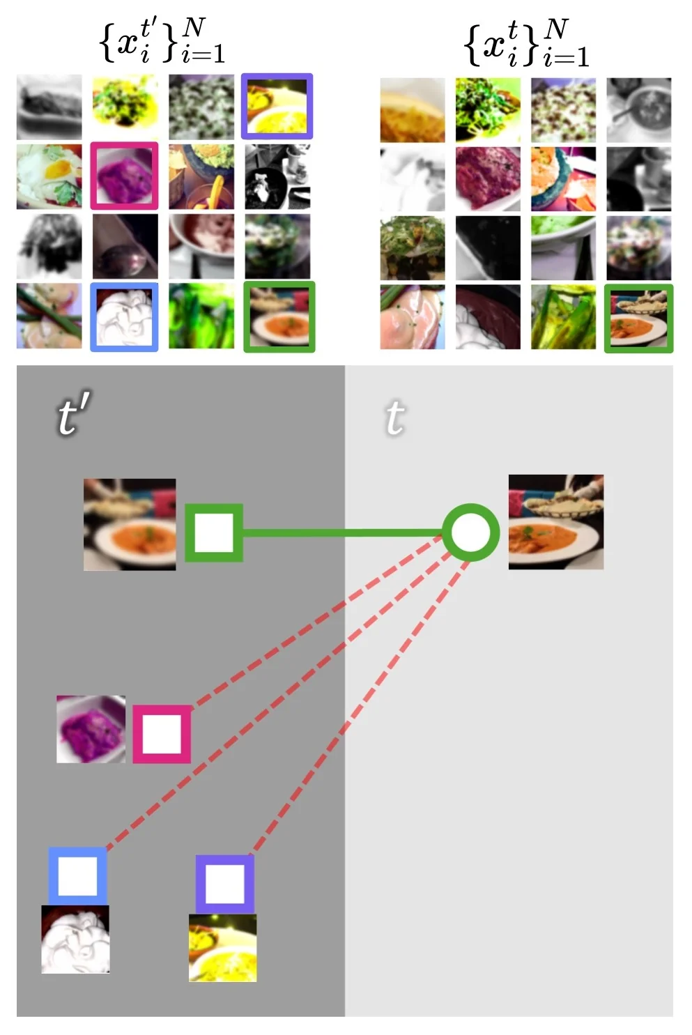
As shown in Figure 22.16, this formulation pulls together positive pairs across augmentations while pushing apart all negatives in the batch. Unlike binary classification formulations, ReLIC optimizes a softmax distribution over the full batch, which enables fine-grained relational learning.
The target encoder—updated via exponential moving average (EMA) of the online encoder—provides stable reference embeddings throughout training. This softmax-based instance discrimination lays the foundation for the second loss term, which aligns relational belief distributions across augmentations to enforce invariance.
Loss Term 2: KL Regularization for Distributional Invariance While the contrastive objective aligns positive pairs \( (\mathbf {z}_i^t, \mathbf {z}_i^{t'}) \), it does not ensure that the similarity structure of the learned representation is preserved across augmentations. Specifically, two embeddings of the same image—though close to each other—may still rank other samples in the batch differently, resulting in inconsistent relational structure. This undermines the goal of learning augmentation-invariant semantics.
To address this, ReLIC introduces a KL divergence regularization term that promotes distributional invariance: the belief distributions over similarity scores, as induced by different augmentations of the same image, should remain consistent.
KL Divergence Between Positive Pairs. Let \( \mathbf {z}_i^t \) denote the embedding from the online encoder and \( \mathbf {z}_i^{t'} \) from the EMA-updated target encoder. ReLIC defines similarity-based belief distributions as follows:
\[ \begin {aligned} p(x_i^t) &:= p(x_i^t; x_i^{t'}) = \frac {\exp \left ( \phi _\tau (\mathbf {z}_i^t, \mathbf {z}_i^{t'}) \right )}{\sum \limits _{j=1}^N \exp \left ( \phi _\tau (\mathbf {z}_i^t, \mathbf {z}_j^{t'}) \right )} \\[0.5em] p(x_i^{t'}) &:= p(x_i^{t'}; x_i^t) = \frac {\exp \left ( \phi _\tau (\mathbf {z}_i^{t'}, \mathbf {z}_i^t) \right )}{\sum \limits _{j=1}^N \exp \left ( \phi _\tau (\mathbf {z}_i^{t'}, \mathbf {z}_j^t) \right )} \end {aligned} \]
The KL divergence is then computed as: \[ D_{\mathrm {KL}}(p(x_i^t) \,\|\, p(x_i^{t'})) = \mathrm {sg} \left [ \log p(x_i^{t'}; x_i^t) \right ] - \log p(x_i^t; x_i^{t'}) \]
This expression is consistent with the formulation in the original paper. The stop-gradient operator \( \mathrm {sg}[\cdot ] \) is applied to the first term, freezing the target distribution computed from \( \mathbf {z}_i^{t'} \). During training, only the online encoder \( f \) (producing \( \mathbf {z}_i^t \)) is updated, while the target encoder \( g \) (producing \( \mathbf {z}_i^{t'} \)) provides a stable reference distribution.
Rationale for Stop-Gradient. This asymmetry in optimization is crucial. If both sides of the KL divergence were updated simultaneously, they could co-adapt or collapse toward trivial, unstable solutions. By freezing the target-side distribution, ReLIC stabilizes training and ensures that the online encoder learns to match a slowly evolving belief structure. This follows the mean teacher strategy [729], where the EMA encoder serves as a consistent teacher guiding the online encoder toward invariant behavior.
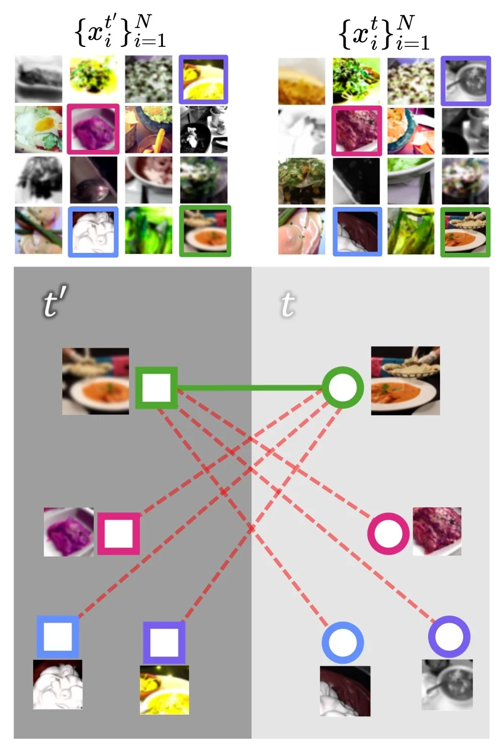
As shown in Figure 22.17, this loss does not merely align a positive pair but enforces that their similarity profiles over the batch remain invariant. This encourages the model to encode consistent relational structure under visual perturbations.
From Causal Motivation to Loss Construction ReLIC is motivated by a causal view of data generation, assuming that an image is generated as:
\[ X = g(C, S), \qquad C \perp S \]
Here, \( C \) represents semantic content (identity), while \( S \) encodes nuisance style factors (e.g., lighting, texture, viewpoint). Augmentations correspond to interventions \( \texttt{do}(S = s) \) that modify style while preserving content. The objective is to learn representations \( f(X) \) that preserve information about \( C \), while being invariant to changes in \( S \):
\[ p^{\mathrm {do}(a)}(Y^R \mid f(X)) \approx \mbox{constant across } a \in \mathcal {A} \]
This leads to a two-part loss:
- First-order consistency: contrastive alignment of positive pairs via instance discrimination.
- Second-order consistency: KL regularization to enforce invariance of similarity beliefs across different augmentations.
ReLIC Objective The full training loss combines contrastive alignment with the KL regularizer:
\[ \mathcal {L}_{\mathrm {ReLIC}} = \sum _{t, t' \sim \mathcal {T}} \sum _{i=1}^{N} \left [ - \log p(x_i^t; x_i^{t'}) + \beta \cdot D_{\mathrm {KL}}(p(x_i^t) \,\|\, p(x_i^{t'})) \right ] \]
Here, the contrastive term aligns positive pairs and repels negatives, while the KL term enforces second-order consistency—i.e., stable similarity distributions across views. The use of random sampling over augmentations \( t, t' \sim \mathcal {T} \) ensures that both asymmetric directions are symmetrized statistically over training.
Though the notations \( p(x_i^t) \) and \( p(x_i^{t'}) \) appear independent, it is critical to recognize that they are inherently cross-view coupled: each belief distribution is computed relative to embeddings from the opposite augmentation stream. This coupling is the cornerstone of ReLIC’s distributional invariance mechanism and is what gives the KL term its power to preserve relational structure under stylistic perturbations.
Architecture and Implementation Details
- Encoders \( f, g \): ResNet-50 backbones
- Projection heads \( h, q \): 4-layer MLPs with hidden sizes decreasing from 4096 to 512
- Representation dimension: 128
- Augmentations: random resized crop, color jitter, blur
- EMA decay: typically \( m = 0.999 \)
Performance and Evaluation ReLIC was shown to perform competitively on ImageNet-1k under the linear evaluation protocol. With ResNet-50, it achieved a top-1 accuracy of 74.8%, surpassing BYOL (74.3%) and approaching SwAV (75.3%) despite using no labels.
Importantly, the target encoder \( g \) was used for downstream tasks—leveraging its stabilized updates for robust representation quality.
Summary and Outlook ReLIC advances contrastive self-supervised learning by formally embedding it within a causal framework and enforcing explicit invariance through regularization. This combination of theory and practice yields robust, transferable features and avoids overfitting to augmentation artifacts. Its success underscores the power of integrating causal reasoning into representation learning.
In the following subsection, we explore ReLICv2 [640], which pushes this principle further through saliency-aware masking, multi-scale augmentations, and more aggressive generalization techniques—achieving state-of-the-art robustness and even surpassing supervised learning baselines.
22.3.9 ReLICv2: Enhanced Invariant Representation Learning
Motivation: From View Invariance to Causal Robustness
While ReLIC [450] introduced a principled invariance regularizer to contrastive learning, it still relied on standard augmentations to simulate causal interventions on style. However, such augmentations may preserve background textures or co-occurring objects that correlate with semantic classes but are not causally related to the object’s identity. These spurious correlations can leak into the learned representations, reducing generalization to out-of-distribution (OOD) data.
ReLICv2 [640] addresses this by incorporating additional methodologies to steer the model toward representations that are truly content-based. Its core aim is to ensure that the similarity structure induced by the learned representation reflects underlying semantic content—regardless of variation in background, style, or partial visibility. To this end, ReLICv2 extends the original framework along two key dimensions:
- 1.
- Foreground-aware saliency masking to remove spurious background signals.
- 2.
- Multi-view training with heterogeneous crop sizes to promote spatial and semantic robustness.
Foreground Saliency Masking
A central challenge in contrastive representation learning is the presence of spurious correlations—for instance, consistent co-occurrence between a semantic object and background artifacts such as textures, lighting conditions, or object co-appearance. While ReLIC [450] addressed this problem by enforcing invariance across augmentations, it treated all pixels equally, which allowed such spurious background features to influence learning.
To counteract this, ReLICv2 [640] introduces a fully unsupervised saliency masking mechanism that encourages learning from foreground content while ignoring distractive background information. This is achieved through the following steps:
- A saliency estimation pipeline is applied to each view during training to generate a binary mask.
- Pixels outside salient regions are masked out and replaced by noise or zero.
- This operation is applied stochastically, so some crops retain full background information to preserve diversity.
The key advantage of this approach is that the model learns to be invariant to background style by seeing both masked and unmasked variants of the same image and being explicitly penalized if its similarity distribution shifts. This enforces a causal disentanglement between the object’s content and its style or context.
Multi-View Learning with Large and Small Crops
ReLICv2 generalizes the two-view contrastive setup of ReLIC into a flexible multi-view framework that better captures semantic and spatial invariance. Specifically, it samples a set of large views (standard resized crops of the full image) and a smaller number of small views (localized, tighter crops, potentially occluding object parts). The key motivations behind this design are:
- Style robustness: Large views, subjected to heavy augmentations (color jitter, blur, etc.), teach the model to be invariant to style changes while preserving object identity.
- Occlusion robustness: Small views encourage the model to preserve consistent similarity distributions even when only partial visual evidence of the object is available.
ReLICv2 Objective
ReLICv2 extends the original ReLIC framework [450] by combining instance-level contrastive learning with a distributional invariance regularizer. It operates over multiple augmented views of each image in a batch, leveraging both global and local crops. For each image \( x_i \) in a batch of \( N \) training samples, two distinct sets of augmentations are generated:
- \( \mathcal {L}_i = \{ x_i^{l, t_{\ell _1}} \}_{\ell _1=1}^{L} \sim \mathcal {T}_{\mbox{sal}} \): a set of \( L \) large (global) views per image, where each augmentation \( t_{\ell _1} \sim \mathcal {T}_{\mbox{sal}} \) applies standard transformations from \( \mathcal {T} \) with optional saliency masking (with probability \( p_m \)). These large views serve both as online queries and as targets via the EMA network. In the loss, one of them—indexed by \( \ell _1 \)—acts as the reference anchor.
- \( \mathcal {S}_i = \{ x_i^{s, t_{s_1}} \}_{s_1=1}^{S} \sim \mathcal {T} \): a set of \( S \) small (local) views, where each augmentation \( t_{s_1} \sim \mathcal {T} \) uses standard SimCLR-style transformations without masking. These are used only as queries through the online encoder.
Each view \( x \in \mathcal {L}_i \cup \mathcal {S}_i \) is passed through the online encoder-projector \( h(f(x)) \), yielding an \( \ell _2 \)-normalized query embedding \( \mathbf {z} \in \mathbb {R}^d \). However, only the large views \( x_i^{l, t_{\ell _1}} \in \mathcal {L}_i \) are also processed by the EMA-based target network \( q(g(x)) \) to produce corresponding target embeddings \( \mathbf {z}' \in \mathbb {R}^d \). This design reflects a key idea: large views are more likely to preserve global object semantics and full spatial context, making them better suited as stable targets.
In contrast, small crops may omit critical semantic information and thus are excluded from forming targets to prevent anchoring on incomplete or misleading features.
The total ReLICv2 objective combines contrastive identification and distributional alignment across multiple augmented views of each image: \begin {align} \mathcal {L} = \sum _{i=1}^{N} \sum _{\ell _1=1}^{L} \Bigg ( &\underbrace { \sum _{\ell _2=1}^{L} \left [ \underbrace {- \log p(x_i^{l, t_{\ell _2}}; x_i^{l, t_{\ell _1}})}_{\substack {\text {large-to-large}\\\text {contrastive}}} + \underbrace {\beta \cdot D_{\mathrm {KL}}\left (p(x_i^{l, t_{\ell _2}}) \parallel \operatorname {sg}[p(x_i^{l, t_{\ell _1}})]\right )}_{\substack {\text {large-to-large}\\\text {distributional alignment}}} \right ] }_{\substack {\text {comparisons among}\\\text {large views}}} \nonumber \\ &+ \underbrace { \sum _{s_1=1}^{S} \left [ \underbrace {- \log p(x_i^{s, t_{s_1}}; x_i^{l, t_{\ell _1}})}_{\substack {\text {small-to-large}\\\text {contrastive}}} + \underbrace {\beta \cdot D_{\mathrm {KL}}\left (p(x_i^{s, t_{s_1}}) \parallel \operatorname {sg}[p(x_i^{l, t_{\ell _1}})]\right )}_{\substack {\text {small-to-large}\\\text {distributional alignment}}} \right ] }_{\substack {\text {comparisons of small views}\\\text {to large anchor } x_i^{l, t_{\ell _1}}}} \Bigg ) \label {eq:chapter22_relicv2_loss} \end {align}
As indicated in Eq. (22.1), large views appear on both sides of the probability terms—once as queries through the online network and once as targets through the EMA network—whereas small views appear only on the query side. This asymmetry is deliberate. Large crops typically cover most of the object and its surrounding context, so restricting the EMA network to these views makes its targets encode stable, holistic semantics. Letting the same large views also act as queries ties the online representation space to this global anchor, ensuring that the online encoder cannot drift too far from a context-rich reference. Small crops, by contrast, may capture only object parts or even background. They are therefore used solely as queries, never as targets, so that incomplete or ambiguous content cannot reshape the EMA distribution. Moreover, the objective intentionally omits small-to-small terms: local views are never trained to match one another directly, but instead are all pulled toward the shared large-view targets via the InfoNCE and KL components. In effect, each small crop must explain the same global semantic distribution as its corresponding large view, enforcing a local-to-global inductive bias while keeping the target side anchored in stable, high-level structure.
Term 1: Contrastive Log-Likelihood (Large-to-Large) The first component of the ReLICv2 loss in Equation (22.1) compares large (global) views of the same image under different augmentations. For each training image \( x_i \), each large view \( x_i^{l, t_{\ell _2}} \in \mathcal {L}_i \) is treated as a query, and compared to a designated reference anchor \( x_i^{l, t_{\ell _1}} \in \mathcal {L}_i \). The online and target embeddings are given by: \[ \mathbf {z} = h(f(x_i^{l, t_{\ell _2}})), \quad \mathbf {z}' = q(g(x_i^{l, t_{\ell _1}})), \] where all vectors are \( \ell _2 \)-normalized. The similarity between query and target is computed using a temperature-scaled dot product: \[ \phi _\tau (\mathbf {z}, \mathbf {z}') = \frac {\langle \mathbf {z}, \mathbf {z}' \rangle }{\tau }. \]
To estimate the contrastive likelihood, ReLICv2 defines a candidate set \( \mathcal {C}_i^{l, \ell _2} = \{ x_i^{l, t_{\ell _1}} \} \cup \mathcal {N}_i \), where \( \mathcal {N}_i \subset \bigcup _{j \neq i} \mathcal {L}_j \) consists of negative large views sampled from other images in the batch. The contrastive softmax probability of matching query \( x_i^{l, t_{\ell _2}} \) to anchor \( x_i^{l, t_{\ell _1}} \) is: \[ p(x_i^{l, t_{\ell _2}}; x_i^{l, t_{\ell _1}}) = \frac { \exp \left ( \phi _\tau (\mathbf {z}, \mathbf {z}') \right ) }{ \sum \limits _{x_k \in \mathcal {C}_i^{l, \ell _2}} \exp \left ( \phi _\tau (\mathbf {z}, \mathbf {z}'_k) \right ) }, \] where \( \mathbf {z}'_k = q(g(x_k)) \) are target embeddings of the candidates. The negative log-likelihood loss, \[ - \log p(x_i^{l, t_{\ell _2}}; x_i^{l, t_{\ell _1}}), \] encourages alignment between different large views of the same image while contrasting against negatives from other images.
A corresponding contrastive term is also applied between each small view \( x_i^{s, t_{s_1}} \in \mathcal {S}_i \) and the same anchor \( x_i^{l, t_{\ell _1}} \). This will be described in detail in later parts.
Term 2: KL Divergence (Large-to-Large) The second component of the large-to-large comparison in Equation (??) enforces distributional invariance between augmented views of the same image. Rather than matching a single positive, this term aligns entire similarity distributions over the batch, thereby promoting second-order consistency in relational structure.
Let \( x_i^{l, t_{\ell _2}} \in \mathcal {L}_i \) be the query view, and \( x_i^{l, t_{\ell _1}} \in \mathcal {L}_i \) the reference anchor. The online embedding of the query is: \[ \mathbf {z}_{\mbox{query}} = h(f(x_i^{l, t_{\ell _2}})), \] while the online embedding of the reference view is: \[ \mathbf {z}_{\mbox{ref}} = h(f(x_i^{l, t_{\ell _1}})). \] To compute similarity distributions, both embeddings are compared to a shared candidate set of target embeddings defined over the current batch: \[ \mathcal {K}_{\mbox{batch}} = \left \{ q(g(x_k)) \;\middle |\; x_k \in \bigcup _{j=1}^N \mathcal {L}_j \right \}. \] For each candidate \( \mathbf {z}'_k \in \mathcal {K}_{\mbox{batch}} \), we define the similarity between the query and candidate as: \[ \phi _\tau (\mathbf {z}, \mathbf {z}'_k) = \frac {\langle \mathbf {z}, \mathbf {z}'_k \rangle }{\tau }. \]
The resulting similarity distributions over \(\mathcal {K}_{\mbox{batch}}\) are defined as softmaxes: \begin {align*} p(x_i^{l, t_{\ell _2}})[k] &= \frac { \exp \left ( \phi _\tau (\mathbf {z}_{\text {query}}, \mathbf {z}'_k) \right ) }{ \sum \limits _{\mathbf {z}'_{k'} \in \mathcal {K}_{\text {batch}}} \exp \left ( \phi _\tau (\mathbf {z}_{\text {query}}, \mathbf {z}'_{k'}) \right ) }, \\ p(x_i^{l, t_{\ell _1}})[k] &= \frac { \exp \left ( \phi _\tau (\mathbf {z}_{\text {ref}}, \mathbf {z}'_k) \right ) }{ \sum \limits _{\mathbf {z}'_{k'} \in \mathcal {K}_{\text {batch}}} \exp \left ( \phi _\tau (\mathbf {z}_{\text {ref}}, \mathbf {z}'_{k'}) \right ) }. \end {align*}
The KL divergence between these two distributions is then: \[ D_{\mathrm {KL}}\left ( p(x_i^{l, t_{\ell _2}}) \,\|\, \operatorname {sg}[p(x_i^{l, t_{\ell _1}})] \right ), \] where the stop-gradient operator \( \operatorname {sg}[\cdot ] \) freezes the reference distribution to prevent gradient flow. This ensures that the online embedding of the query view learns to imitate the relational structure of the anchor without altering the target distribution.
In combination with the contrastive term, this distributional alignment encourages each large view to exhibit consistent similarity rankings to all other examples, thereby reinforcing invariance to augmentation, masking, and local variation.
Small-to-Large View Consistency Terms In addition to large-to-large comparisons, ReLICv2 enforces consistency between small (local) and large (global) views of the same image. These terms correspond to the second set of inner summands in Equation (22.1), where each small view \( x_i^{s, t_{s_1}} \in \mathcal {S}_i \) is aligned to a large anchor view \( x_i^{l, t_{\ell _1}} \in \mathcal {L}_i \) using both contrastive and distributional losses.
Let \[ \mathbf {z}_{\mbox{query}} = h(f(x_i^{s, t_{s_1}})) \] denote the online embedding of the small view, and \[ \mathbf {z}_{\mbox{ref}} = h(f(x_i^{l, t_{\ell _1}})) \] the online embedding of the reference large view. The target candidate set remains \[ \mathcal {K}_{\mbox{batch}} = \left \{ \mathbf {z}'_k = q(g(x_k)) \;\middle |\; x_k \in \bigcup _{j=1}^N \mathcal {L}_j \right \}, \] where each \( \mathbf {z}'_k \in \mathbb {R}^d \) is the \( \ell _2 \)-normalized target embedding corresponding to a large view in the batch.
The contrastive softmax probability that the small view matches its designated large anchor is: \[ p(x_i^{s, t_{s_1}}; x_i^{l, t_{\ell _1}}) = \frac { \exp \left ( \phi _\tau (\mathbf {z}_{\mbox{query}}, \mathbf {z}'_{\ell _1}) \right ) }{ \sum \limits _{\mathbf {z}'_k \in \mathcal {K}_{\mbox{batch}}} \exp \left ( \phi _\tau (\mathbf {z}_{\mbox{query}}, \mathbf {z}'_k) \right ) }, \]
where \( \mathbf {z}'_{\ell _1} = q(g(x_i^{l, t_{\ell _1}})) \) is the target embedding of the anchor view. The corresponding first-order contrastive loss is: \[ - \log p(x_i^{s, t_{s_1}}; x_i^{l, t_{\ell _1}}), \] which encourages the small view to identify the correct global anchor among a set of distractors from other images.
To additionally enforce second-order alignment, similarity distributions over the batch are computed for both views: \begin {align*} p(x_i^{s, t_{s_1}})[k] &= \frac { \exp \left ( \phi _\tau (\mathbf {z}_{\text {query}}, \mathbf {z}'_k) \right ) }{ \sum \limits _{\mathbf {z}'_{k'} \in \mathcal {K}_{\text {batch}}} \exp \left ( \phi _\tau (\mathbf {z}_{\text {query}}, \mathbf {z}'_{k'}) \right ) }, \\ p(x_i^{l, t_{\ell _1}})[k] &= \frac { \exp \left ( \phi _\tau (\mathbf {z}_{\text {ref}}, \mathbf {z}'_k) \right ) }{ \sum \limits _{\mathbf {z}'_{k'} \in \mathcal {K}_{\text {batch}}} \exp \left ( \phi _\tau (\mathbf {z}_{\text {ref}}, \mathbf {z}'_{k'}) \right ) }, \end {align*}
for all \( \mathbf {z}'_k \in \mathcal {K}_{\mbox{batch}} \). These distributions reflect the relational structure induced by each view across the batch.
The KL divergence term between the distributions is: \[ D_{\mathrm {KL}}\left ( p(x_i^{s, t_{s_1}}) \,\|\, \operatorname {sg}[p(x_i^{l, t_{\ell _1}})] \right ), \] where the stop-gradient operator \( \operatorname {sg}[\cdot ] \) ensures that the reference distribution remains fixed during optimization. This term aligns the similarity profile of the partial view with that of the full-resolution anchor, reinforcing relational consistency.
Together, these small-to-large alignment terms promote local-to-global consistency, requiring representations of cropped or occluded views to exhibit the same relational semantics as their corresponding full-image counterparts. This increases robustness to object scale, partial visibility, and spatial perturbations.
Training Procedure The pseudocode below summarizes the training pipeline for ReLICv2. Each batch sample \( x \) is optionally passed through a learned saliency masking module to suppress background regions with probability \( p_m \). Large views are generated via global crops and passed through both the online network \( f_o \) and the target network \( g_t \), while small views are generated via local crops and passed only through \( f_o \). The online and target projections are then used to compute the ReLICv2 loss, which includes both contrastive log-likelihood and KL divergence terms for all large-to-large and small-to-large view pairs, as defined in Equation (22.1).
After computing the average loss over all view comparisons, the online network is updated via backpropagation, and the target network is updated using an exponential moving average (EMA) of the online parameters. This view-dependent asymmetry ensures that only semantically complete views contribute to the distributional anchors, while smaller or occluded views regularize the learning objective.
’’’
f_o: online network: encoder + comparison_net
g_t: target network: encoder + comparison_net
gamma: target EMA coefficient
n_e: number of negatives
p_m: mask apply probability
’’’

for x in batch:  # load a batch of B samples
    # Apply saliency mask and remove background
    x_m = remove_background(x)

    for i in range(num_large_views):
        # Select either original or background-removed image with probability p_m
        x_sel = x_m if Bernoulli(p_m) else x
        # Apply large crop and augmentation
        xl_i = aug(crop_l(x_sel))

        # Forward pass through online and target networks
        ol_i = f_o(xl_i)
        tl_i = g_t(xl_i)

    for i in range(num_small_views):
        # Apply small crop and augmentation
        xs_i = aug(crop_s(x))
        # Forward pass through online network only
        os_i = f_o(xs_i)

    loss = 0

    # Contrastive + KL loss: large-to-large
    for i in range(num_large_views):
        for j in range(num_large_views):
            loss += loss_relic(ol_i, tl_j, n_e)

    # Contrastive + KL loss: small-to-large
        for i in range(num_small_views):
            for j in range(num_large_views):
            loss += loss_relic(os_i, tl_j, n_e)

    # Normalize loss over all pairs
    scale = (num_large_views + num_small_views) * num_large_views
    loss /= scale

    # Backpropagation and EMA update
    loss.backward()
    update(f_o)
    g_t = gamma * g_t + (1 - gamma) * f_o
With the training procedure and loss structure established, we next examine the empirical behavior of ReLICv2 across architectural ablations, saliency effectiveness, and transfer benchmarks.
Empirical Evaluation and Robustness Analysis Continuing from the objective formulation, we now elaborate on the empirical insights, ablations, and evaluation results that highlight the advantages of ReLICv2. These include improvements in robustness, semantic fidelity, and transferability, as well as quantitative comparisons with previous state-of-the-art contrastive methods.
Linear Evaluation Performance ReLICv2 achieves state-of-the-art accuracy under the linear probing protocol on ImageNet, outperforming both self-supervised and fully supervised ResNet-50 models.
ReLICv2 is the first self-supervised method to consistently outperform supervised training on ImageNet under equivalent evaluation settings.
Robustness and Out-of-Distribution Generalization To evaluate the robustness and OOD generalization capabilities of ReLICv2, the authors test linear classifiers trained on frozen ImageNet-pretrained ResNet-50 features across five datasets. The evaluation follows a zero-shot linear protocol: classifiers are trained using labeled ImageNet training data and evaluated directly on the test sets of each benchmark without fine-tuning.
ReLICv2 achieves state-of-the-art robustness across all ImageNet-V2 variants and ImageNet-C, outperforming both previous self-supervised methods and the supervised baseline. For out-of-distribution generalization, ReLICv2 remains competitive with the supervised model and consistently improves upon earlier contrastive approaches.
Semantic Clarity and Class-wise Consistency Beyond accuracy, ReLICv2 improves the semantic structure of the learned feature space, as evidenced by class confusion metrics and visualization.
The improved class separability reflects tighter within-class clustering and more discriminative, content-aligned representations.
Summary
ReLICv2 extends contrastive self-supervised learning with principled causal regularization, saliency masking, and multi-scale view consistency. Its empirical performance not only surpasses earlier methods like ReLIC, MoCo, and SimCLR, but also matches or exceeds supervised learning on ImageNet and robustness benchmarks. These advances underscore the strength of explicit distributional invariance and inductive view diversity in driving generalizable feature learning.
22.3.10 Further Contrastive Innovations
Contrastive learning has progressed significantly beyond its foundational frameworks like SimCLR and MoCo, which rely on instance discrimination with simple augmentations and view matching. Recent approaches have introduced new ways to define “positives” and “negatives,” enhancing sample efficiency, semantic alignment, and robustness to augmentations. This subsection highlights three such innovations: Nearest-Neighbor Contrastive Learning (NNCLR), Adversarial Contrastive Learning (AdCo), and Contrastive Learning with Stronger Augmentations (CLSA).
Nearest-Neighbor Contrastive Learning (NNCLR) NNCLR [139] introduces a principled rethinking of how positive pairs are defined in contrastive learning. Instead of relying solely on augmentations of the same image, NNCLR retrieves the nearest neighbor of each query from a momentum-encoded support queue and uses it as the positive. This shifts the learning objective from enforcing low-level augmentation invariance toward learning semantic consistency across the dataset.
The training process proceeds in three stages:
- 1.
- Two augmented views \( x_i^1, x_i^2 \sim \mathcal {T} \) are generated for each image \( x_i \). One is selected as the query.
- 2.
- The nearest neighbor of the query embedding is retrieved from a dynamically updated support queue to serve as the positive.
- 3.
- An InfoNCE contrastive loss is applied between the query and its nearest neighbor, using other samples from the batch or queue as negatives. Optionally, the loss can be symmetrized by repeating the process with the roles reversed.
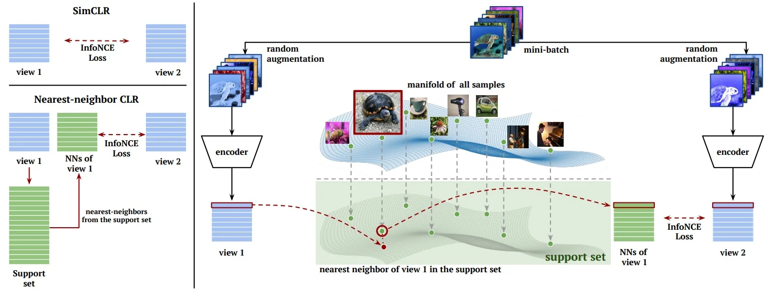
This design introduces several key benefits:
- It promotes semantic grouping: nearest neighbors increasingly belong to the same class or share meaningful visual attributes as training progresses.
- It reduces dependence on strong augmentations, since neighbor retrieval introduces natural variation and semantic diversity.
- It enhances generalization and transferability, improving performance on both linear evaluation and few-shot classification across downstream tasks.
NNCLR improves SimCLR’s ImageNet top-1 accuracy by 3.8% and outperforms supervised ResNet-50 in 11 out of 12 transfer benchmarks.
Adversarial Contrastive Learning (AdCo) AdCo [245] reframes negative sampling as a learnable adversarial process. Instead of drawing negatives from a memory bank or batch, AdCo introduces a set of adversarial negatives—learnable vectors optimized to be maximally confusing to the encoder. Training proceeds via a minimax game: \[ \min _{\theta } \max _{\mathcal {N}} \mathcal {L}_{\mbox{contrast}}(\theta , \mathcal {N}), \] where the encoder \( \theta \) is trained to discriminate positives from negatives, while the adversarial negatives \( \mathcal {N} \) are simultaneously updated to increase their similarity to the query.
This setup provides several key advantages:
- Principled hard negative mining: negatives are dynamically optimized to match the current query distribution.
- Reduced reliance on large batches or queues: learned negatives eliminate the need for external storage or large-scale sampling.
- Improved representation quality: the continual adversarial challenge accelerates convergence and sharpens instance discrimination.
AdCo achieves 75.7% top-1 accuracy on ImageNet (ResNet-50) with multi-crop augmentations, surpassing many memory-based contrastive baselines while using fewer resources.
Contrastive Learning with Stronger Augmentations (CLSA) CLSA [695] addresses a core failure mode of contrastive learning under overly strong augmentations. Traditional objectives force embeddings of weak and strongly augmented views to match directly, risking semantic distortion or collapse. Instead, CLSA compares their similarity distributions over a memory bank, enabling robustness to heavy transformations without enforcing brittle pointwise alignment.
Given a weak view \( z_i^{\mbox{weak}} \) and a strong view \( z_i^{\mbox{strong}} \), CLSA minimizes a distributional KL divergence: \[ \mathcal {L}_{\mbox{DDM}} = \mathrm {KL}\left (p(\cdot \mid z_i^{\mbox{weak}}) \parallel p(\cdot \mid z_i^{\mbox{strong}})\right ), \] where \( p(\cdot \mid z) \) denotes a softmax over cosine similarities to entries in a memory bank. A stop-gradient is applied to the weak-view distribution, distilling its similarity structure into the strong view. This Distributional Divergence Minimization (DDM) loss transfers relational knowledge rather than requiring exact feature alignment.
This design enables:
- Semantic consistency under severe augmentations, by aligning distributions rather than embeddings.
- Robust, generalizable features without collapse, even when weak and strong views differ substantially.
- Improved downstream performance, particularly for detection and transfer settings.
CLSA achieves 76.2% top-1 accuracy on ImageNet with a ResNet-50 backbone and multi-crop augmentation, approaching supervised performance. On COCO, it improves small-object detection AP by 3.6% over MoCo v2, demonstrating strong transferability and robustness.
Enrichment 22.3.10.1: CLSA vs. ReLIC: KL Divergence in Perspective
While both CLSA and ReLICv1 employ KL divergence to align distributions across augmented views, they do so under fundamentally different assumptions and goals. The divergence in purpose is not due to how the distributions are computed—both apply softmax over similarities—but in what those distributions represent and how they are interpreted within the learning process.
CLSA: Distributional Distillation Across Augmentation Strength CLSA [695] addresses the difficulty of learning from strongly augmented views, which may distort semantic content. It applies KL divergence between the similarity distributions of a weakly augmented view \( z_i^{\mbox{weak}} \) and a strongly augmented view \( z_i^{\mbox{strong}} \): \[ \mathcal {L}_{\mbox{DDM}} = \mathrm {KL}\left (p(\cdot \mid z_i^{\mbox{weak}}) \parallel p(\cdot \mid z_i^{\mbox{strong}})\right ), \] where \( p(\cdot \mid z) \) is a softmax over similarities to entries in a memory bank. A stop-gradient is applied to the weak view, casting it as a teacher. The KL term thus distills structural information—i.e., the neighborhood of similar samples—into the strong view. This setup is intentionally asymmetric: the strong view learns from the more stable similarity beliefs of the weak view without forcing their embeddings to match directly.
ReLICv1: Invariant Prediction Across Augmentations ReLICv1 [450] uses KL divergence to enforce prediction consistency across augmented views. Given embeddings from two views \( x_i^t \) and \( x_i^{t'} \), ReLIC aligns their proxy-target prediction distributions: \[ \mathcal {D}_{\mbox{KL}} = \mathrm {KL}\left (p(x_i^t) \parallel \operatorname {sg}[p(x_i^{t'})]\right ), \] where \( p(x) \) is a contrastive softmax over a designated positive and batch negatives. Unlike CLSA, the two views are treated symmetrically in principle—they are semantically equivalent—and the KL term acts as a regularizer for causal invariance. The model is penalized when stylistic changes (augmentations) alter its output belief about the target. The stop-gradient ensures that gradients flow only through the query view, anchoring the prediction distribution of one view as the reference.
Two KL Terms, Two Philosophies
| Aspect | CLSA (DDM Loss) | ReLICv1 (Invariance Loss) |
|---|---|---|
| Input Assumption | Strong view is a degraded student; weak view is the teacher. | Both views are peers; neither is privileged. |
| What is aligned? | Similarity distribution over memory bank neighbors. | Proxy-target prediction over contrastive positives/negatives. |
| Purpose of KL | Guided distillation under heavy augmentation. | Regularization for prediction stability. |
| Role of stop-gradient | On the teacher (weak view). | On the reference view in KL. |
| Underlying Robustness | Robustness through neighborhood consistency. | Causal invariance across style interventions. |
Summary (CLSA vs. ReLIC) Although both methods compare softmax distributions over similarity scores, their roles in learning are distinct. CLSA uses KL divergence for structure transfer from clean to noisy views, enhancing robustness under severe augmentation. ReLIC uses KL divergence for semantic invariance, ensuring that the model’s proxy predictions remain stable across augmentations. Both are asymmetric, but for different reasons—CLSA’s asymmetry reflects a teacher-student hierarchy; ReLIC’s enforces consistency between symmetric peers. This difference reflects their respective goals: relational robustness versus predictive invariance.
Comparative Landscape and Emerging Trends
| Method | Backbone | Negatives? | Positives | Top-1 (%) |
|---|---|---|---|---|
| SimCLR [89] | ResNet-50 | In-batch | Augmented view | 69.3 |
| MoCo v1 [220] | ResNet-50 | Queue | Augmented view | 60.6 |
| MoCo v2 [96] | ResNet-50 | Queue | Augmented view | 71.1 |
| MoCo v3 [94] | ViT-B/16 | Momentum encoder | Augmented view | 76.5 |
| NNCLR [139] | ResNet-50 | NN queue | Nearest neighbor | 75.4 |
| AdCo [245] | ResNet-50 | Adversarial negatives | Augmented view | 72.8 |
| CLSA [695] | ResNet-50 | Queue | Weak/strong views | 76.2 |
| ReLIC [450] | ResNet-50 | Belief alignment | Predictive views | 74.8 |
| ReLICv2 [640] | ResNet-50 | EMA + multi-view | Multi-view + masking | 77.1 |
Across these methods, several trends emerge:
- Semantic alignment via feature-space neighbors (NNCLR).
- Learnable negatives for harder optimization (AdCo).
- Distributional robustness to augmentation strength (CLSA).
These directions extend the original contrastive learning paradigm toward methods that generalize better, converge faster, and are more robust to practical training conditions.
A Transition Toward Natural Supervision While the above methods operate entirely in the visual modality, a growing class of contrastive frameworks leverages image–text supervision. The CLIP model (Contrastive Language–Image Pretraining), introduced in the next section, aligns vision and language encoders via large-scale web supervision, enabling zero-shot transfer and multimodal generalization.
22.3.11 CLIP: Learning Transferable Visual Models from Natural Language Supervision
Motivation: Beyond Fixed Labels Traditional supervised vision models are trained on fixed, human-curated label sets like ImageNet. While effective within their domains, these models suffer two key limitations: they cannot generalize beyond the predefined label set, and they require extensive manual annotation. For example, a model trained on ImageNet may recognize a “leopard,” but not a “hedgehog,” “sedan,” or “birthday cake” if such categories were excluded from training.
The internet, by contrast, offers a vast, freely available resource of images paired with natural language captions—on platforms like Flickr, Reddit, and Pinterest. These (image, text) pairs encode rich, descriptive, and diverse supervision. CLIP [513] proposes to leverage this organic data to train vision models in a more scalable, generalizable, and label-free way: by aligning images and language directly.
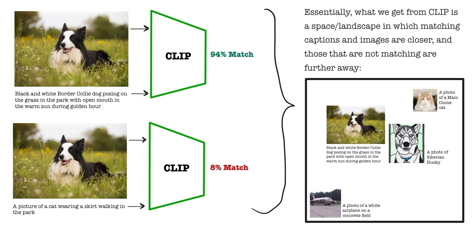
A Naïve Approach: Caption Prediction A natural first attempt to link vision and language is to train a model to generate a caption from an image—similar to traditional image captioning [669]. This seems promising at first: to succeed, the model must learn rich visual semantics. For instance, recognizing that the image in Figure 22.23 depicts a black-and-white Border Collie on grass implies some level of object understanding.
However, this predictive approach quickly proves inefficient for learning general-purpose visual representations. The task of full caption generation is a high-entropy objective: the model must not only parse visual content but also master grammar, syntax, and word ordering. Worse, there are often many valid ways to describe the same image (e.g., “a dog in a field” vs. “a Border Collie outdoors”), making learning brittle—small phrasing changes can yield very different loss signals.
Additionally, captions scraped from the web tend to be noisy, inconsistent, or stylistically verbose (e.g., “A photo of a ...”), further degrading training robustness. These issues compound to make caption prediction a poor pretraining signal for transferable visual understanding.
Efficiency Comparison: Contrastive vs. Predictive Objectives The limitations of prediction-based learning become especially apparent in zero-shot settings—where the model must generalize to new categories without any task-specific supervision. A standard benchmark for evaluating this generalization is zero-shot ImageNet classification.
What is Zero-Shot ImageNet Accuracy? The goal is to classify a test image into one of 1,000 ImageNet classes, without training on labeled ImageNet examples. Rather than learning a classifier, the model performs retrieval over text descriptions:
- 1.
- For each class (e.g., golden retriever, container ship), a prompt such as “a photo of a golden retriever” is written.
- 2.
- These 1,000 prompts are encoded using the model’s text encoder.
- 3.
- The test image is encoded with the image encoder.
- 4.
- The predicted label is the one whose text embedding is closest to the image embedding (typically using cosine similarity).
This evaluation setup naturally favors models that embed both modalities into a shared semantic space—as is the case with CLIP. In contrast, predictive models such as caption generators and Bag-of-Words predictors were originally designed for different objectives and typically require additional adaptation or heuristic matching to be evaluated in this retrieval-style framework.
Figure 22.24 compares three paradigms under this shared evaluation task:
- 1.
- Caption Prediction: Autoregressive models are trained to generate full captions from image inputs. For zero-shot classification, the model first generates a caption, then this caption is matched to one of the 1,000 class prompts—either by computing string or embedding similarity. However, this is a two-stage workaround not aligned with the original training objective. Moreover, autoregressive generation is inherently slow and computationally costly, making this pipeline brittle and inefficient.
- 2.
- Bag-of-Words Prediction: These models output an unordered set of words associated with the image. To adapt this to classification, each class name is reduced to a bag of tokens, and the model’s prediction is matched by measuring overlap (e.g., Jaccard similarity or word count). This formulation removes syntax and speeds up training—achieving a \(3\times \) efficiency gain over full captioning—but it still lacks a true similarity metric or embedding space for semantic alignment, limiting performance.
- 3.
- Contrastive Learning (CLIP): CLIP directly learns a joint embedding space by maximizing agreement between paired image–text embeddings in a batch of \(N\) pairs. Using a symmetric contrastive loss, the model distinguishes \(N\) correct alignments from \(N^2\) possibilities. This not only fits the zero-shot retrieval formulation exactly—it also yields an additional \(4\times \) efficiency gain over Bag-of-Words, and a total of \(12\times \) over caption generation.
Why Contrastive Learning Wins CLIP’s alignment of training objective, architecture, and evaluation yields several key advantages:
- No generation overhead. CLIP bypasses the need for text decoding, grammar modeling, or syntactic correctness—only vector similarity matters.
- Direct semantic grounding. Because learning is framed as matching, CLIP aligns image and text by shared meaning, not lexical overlap—making it robust to phrasing variation.
- Superior generalization. CLIP achieves state-of-the-art zero-shot accuracy on ImageNet without ever seeing the 1,000 labels—demonstrating contrastive learning’s strength for transfer.
Key Insight While all three approaches leverage similar image–text data, only CLIP’s contrastive formulation is structurally aligned with retrieval-based classification. Predictive models like caption generators and Bag-of-Words predictors require nontrivial adaptations to operate in this setting, often resulting in inefficiencies and mismatches between their training and evaluation procedures. CLIP, by contrast, is trained end-to-end to embed images and text into a shared semantic space, where simple similarity comparisons drive both training and inference.
This alignment between objective and evaluation is what enables CLIP to outperform traditional models in both accuracy and efficiency. But how exactly is this achieved? In the next parts, we explore the architectural design and training strategy that make CLIP’s contrastive learning pipeline so effective—and so broadly applicable.
CLIP’s Contrastive Training Approach and Loss
Training Strategy: Paired Alignment at Scale CLIP is trained to align images and their natural language descriptions in a shared multimodal embedding space using a contrastive objective. Its architecture consists of two independent yet jointly optimized encoders:
- An image encoder \( f_{\mbox{img}} \), typically a ResNet-50 or Vision Transformer (ViT), maps an image \( x_i^{\mbox{img}} \) to a latent representation. A learned projection head \( W_{\mbox{img}} \) then maps this representation into the shared embedding space.
- A text encoder \( f_{\mbox{text}} \), implemented as a Transformer with causal attention (similar to GPT), maps a sequence of tokens \( x_i^{\mbox{text}} \) to a text representation. Like the image side, it is followed by a projection head \( W_{\mbox{text}} \) to align the embedding space. Importantly, this encoder is trained from scratch alongside the vision backbone—without using language-specific objectives like masked language modeling or next-token prediction.
Both embeddings are \(\ell _2\)-normalized to lie on the unit hypersphere: \[ \mathbf {z}_i^{\mbox{img}} = \mbox{normalize}(f_{\mbox{img}}(x_i^{\mbox{img}}) W_{\mbox{img}}), \quad \mathbf {z}_i^{\mbox{text}} = \mbox{normalize}(f_{\mbox{text}}(x_i^{\mbox{text}}) W_{\mbox{text}}) \] This ensures that similarity between representations corresponds directly to their cosine similarity, computed as a dot product between normalized vectors.
Symmetric Contrastive Loss CLIP optimizes a symmetric contrastive loss over batches of paired image–text examples. Given a batch of \( N \) pairs \( \{(x_i^{\mbox{img}}, x_i^{\mbox{text}})\}_{i=1}^N \), the model considers all \( N^2 \) possible image–text pairings. The similarity between image \( i \) and text \( j \) is given by: \begin {equation} s_{i,j} = \frac {\langle \mathbf {z}_i^{\mbox{img}}, \mathbf {z}_j^{\mbox{text}} \rangle }{\tau } \label {eq:chapter22_clip_similarity} \end {equation} where \( \tau > 0 \) is a learnable temperature parameter that controls the sharpness of the softmax distribution. A lower value of \( \tau \) emphasizes hard negatives more strongly. This is essentially a temperatured cosine similarity, as the embedding vectors are \(\ell _2\)-normalized.
The loss is defined as the average of two cross-entropy terms:
\begin {equation} \mathcal {L}_{\mbox{CLIP}} = \frac {1}{2N} \sum _{i=1}^{N} \left [ - \log \frac {\exp (s_{i,i})}{\sum _{j=1}^{N} \exp (s_{i,j})} - \log \frac {\exp (s_{i,i})}{\sum _{j=1}^{N} \exp (s_{j,i})} \right ] \label {eq:chapter22_clip_loss} \end {equation}
- The first term encourages each image to retrieve its paired text (image-to-text).
- The second encourages each caption to retrieve its corresponding image (text-to-image).
This symmetric setup casts contrastive learning as two parallel classification problems. Each image and caption acts as a query, identifying its matching partner among all candidates in the batch. All other pairs serve as implicit negatives—yielding \( N^2 - N \) distractors per batch.
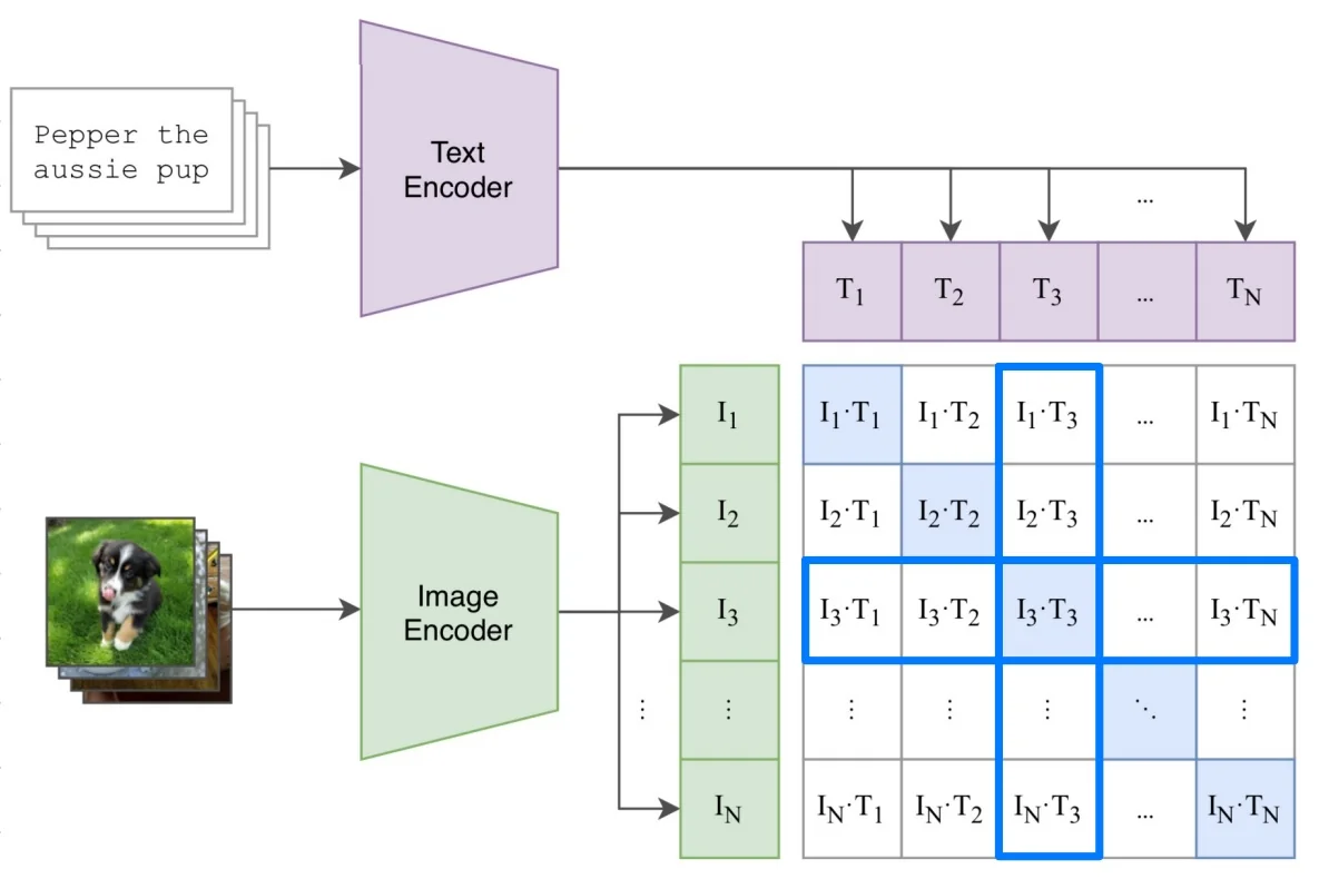
Interpretation and Scaling Advantages CLIP’s contrastive objective directly optimizes semantic alignment across modalities without relying on generation, token-level supervision, or fixed label vocabularies. By training on naturally co-occurring (image, text) pairs, the model learns to encode meaning in a way that is more invariant to phrasing and robust to contextual variation. This approach enables retrieval-based evaluation without requiring textual decoding or classification heads.
Importantly, the shared embedding space learned by CLIP supports efficient downstream usage: zero-shot classification, retrieval, and prompt-based recognition all reduce to simple similarity search via dot products. This stands in contrast to autoregressive captioning or bag-of-words models, which require additional steps—such as text generation or lexical matching—to participate in the same tasks.
Efficient Large-Scale Training CLIP was trained on a massive dataset of 400 million (image, text) pairs collected from the web. The dual-encoder architecture makes this process computationally scalable: contrastive gradients can be computed efficiently across large batches in parallel, without the need for memory banks, hard negative mining, or cross-modal attention mechanisms.
Moreover, CLIP treats the temperature parameter \( \tau \) in the similarity score as a learnable quantity. Rather than manually tuning it, the model optimizes \( \tau \) jointly with the encoders. This dynamic adaptation improves convergence and stability, particularly when training with large and noisy data.
Together, these design choices make CLIP’s training pipeline not only more scalable but also better aligned with real-world web supervision, laying the groundwork for transferable, open-vocabulary visual understanding.
CLIP Loss Pseudo Code & Further Explanations
’’’
image_encoder - ResNet or Vision Transformer(ViT)
text_encoder - CBOW or Text Transformer
I[n, h, w, c] - minibatch of aligned images
T[n, l] - minibatch of aligned texts
W_i[d_i, d_e] - learned projection of image to embed
W_t[d_t, d_e] - learned projection of text to embed
t - learned temperature parameter
’’’

# extract feature representations of each modality:
I_f = image_encoder(I)  # [n, d_i]
T_f = text_encoder(T)  # [n, d_t]

# joint multimodal embedding [n, d_e]:
I_e = l2_normalize(np.dot(I_f, W_i), axis=1)
T_e = l2_normalize(np.dot(T_f, W_t), axis=1)

# scaled pairwise cosine similarities [n, n]:
logits = np.dot(I_e, T_e.T) * np.exp(t)

# symmetric loss function:
labels = np.arange(n)
loss_i = cross_entropy_loss(logits, labels, axis=0)
loss_t = cross_entropy_loss(logits, labels, axis=1)
loss = (loss_i + loss_t)/2
Explanation The input consists of \( N \) aligned (image, text) pairs. The image encoder produces visual feature vectors of dimension \( d_i \), while the text encoder outputs textual features of dimension \( d_t \). These are projected into a shared \( d_e \)-dimensional embedding space using learned linear mappings \( W_i \in \mathbb {R}^{d_i \times d_e} \) and \( W_t \in \mathbb {R}^{d_t \times d_e} \).
Since the raw feature dimensions \( d_i \) and \( d_t \) differ across modalities, the projections \( W_i \) and \( W_t \) ensure compatibility for similarity comparison. After projection, both embeddings are \( \ell _2 \)-normalized, making the dot product a cosine similarity: \[ \mbox{cosine}(z_i^{\mbox{img}}, z_j^{\mbox{text}}) = \frac {\langle z_i^{\mbox{img}}, z_j^{\mbox{text}} \rangle }{\|z_i^{\mbox{img}}\| \cdot \|z_j^{\mbox{text}}\|} = \langle z_i^{\mbox{img}}, z_j^{\mbox{text}} \rangle \] as \( \|z\| = 1 \) after normalization. The resulting matrix of logits \( \in \mathbb {R}^{N \times N} \) contains pairwise similarities scaled by \( \exp (t) \), where \( t \in \mathbb {R} \) is a learned temperature parameter controlling the sharpness of the softmax distribution.
The final loss is symmetric: it computes a softmax distribution over both rows (image-to-text) and columns (text-to-image), applying a cross-entropy objective in each direction:
- Row-wise (Image→Text): For each image embedding, predict the index of its matching caption within the batch.
- Column-wise (Text→Image): For each text embedding, predict the index of its corresponding image.
By penalizing high similarity with mismatched pairs, the loss encourages the model to separate true associations from in-batch negatives. The total loss is the average of the two directional components.
Intuition Behind the BCE Terms The batch cross-entropy (BCE) terms across each axis correspond to estimating a categorical distribution over possible matches. For the image-to-text loss: \[ \mbox{BCE}_i = -\log \frac {\exp (\langle z_i^{\mbox{img}}, z_i^{\mbox{text}} \rangle / \tau )}{\sum _{j=1}^N \exp (\langle z_i^{\mbox{img}}, z_j^{\mbox{text}} \rangle / \tau )} \] The same applies symmetrically for the text-to-image direction. These distributions penalize the model for assigning high confidence to mismatched pairs \( i \neq j \), encouraging tight alignment across modalities.
CLIP Experiments and Ablations
Zero-Shot Performance vs. Supervised Models A key highlight of CLIP’s training pipeline is its ability to perform zero-shot classification—assigning labels to images from unseen datasets without any gradient updates or supervision. To benchmark this, the authors compared zero-shot CLIP models to traditional supervised baselines trained on ImageNet.
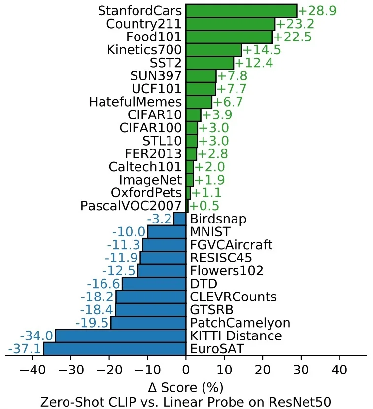
The standard supervised baseline here uses a linear probe: a linear classifier trained atop frozen ResNet-50 representations. CLIP, by contrast, uses zero-shot prompts like “a photo of a banana” to embed classes and selects the class whose embedding has highest cosine similarity with the image. The fact that CLIP can outperform supervised ResNet-50 on ImageNet—without access to ImageNet labels—speaks to the effectiveness of language supervision and contrastive learning at scale.
Notably, CLIP’s margin of superiority is largest on datasets with few training examples per class, where fine-tuning is difficult but general representations are valuable. On highly specialized or medical tasks (e.g., tumor detection), however, supervised models still outperform.
Robustness to Natural Distribution Shift Vision models often suffer substantial performance degradation under natural distribution shift—a change in data appearance or source that does not alter the label space. CLIP, trained on noisy and uncurated web data, displays remarkable robustness in this setting.
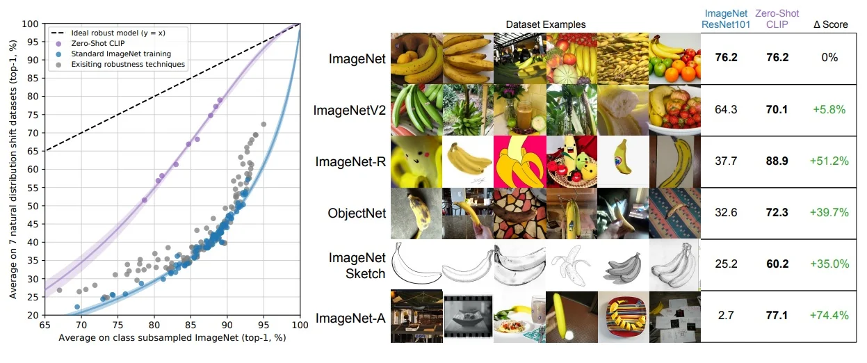
For example, when evaluating image classification across ImageNet and four derived variants (e.g., ImageNet-V2, ImageNet-R, ObjectNet), CLIP maintains stronger consistency than a supervised ResNet-101 with similar in-domain accuracy. The key factor is CLIP’s exposure to diverse, real-world variation during pretraining, which encourages abstraction over spurious correlations. Rather than memorizing style- or dataset-specific statistics, CLIP learns to recognize the underlying semantic identity of objects (e.g., banana-ness) across contexts.
Linear Probe Evaluation Across Models To further probe the quality of its representations, CLIP was evaluated using linear probes on frozen encoders. This is a common technique for comparing feature expressiveness across models: a logistic classifier is trained on top of the frozen embeddings to assess how linearly separable different categories are.
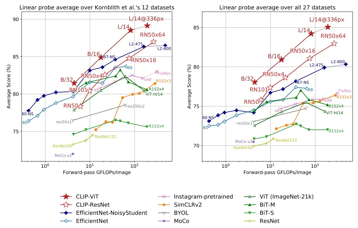
The results demonstrate that CLIP’s representations are broadly transferable: its largest model (ViT-L/14@336px) outperforms strong supervised and self-supervised baselines, such as MoCo v2 and Noisy Student EfficientNet-L2, on both 12- and 27-dataset suites. Additionally, ViT-based CLIP models were found to be roughly \(3\times \) more compute-efficient than CLIP’s ResNet counterparts—highlighting the dual benefits of better generalization and architectural efficiency.
Tradeoffs in Dataset-Specific Adaptation The final experiment explored the tension between generality and specialization. While CLIP excels in zero-shot transfer, adapting it to a specific dataset—via fine-tuning or learning dataset-specific classifiers—can sometimes improve local performance at the cost of broader robustness.
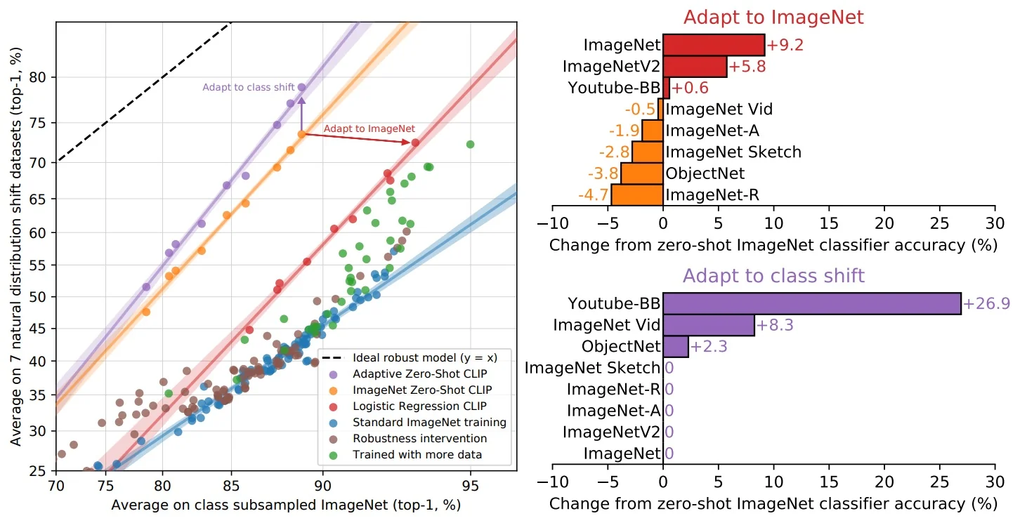
For instance, training a linear classifier directly on ImageNet features can slightly improve classification accuracy on ImageNet itself, but may lower performance on distribution shift benchmarks. This suggests that such fine-tuning encourages reliance on domain-specific cues. The authors recommend using prompt ensembling (e.g., averaging over templates like “a photo of a {label}”) to boost zero-shot accuracy while preserving generalization.
Summary and Practical Takeaways CLIP’s experimental evaluation reinforces the power of contrastive language–image pretraining on noisy, web-scale data. Its design decisions—such as symmetric contrastive loss, massive in-batch negatives, and a learnable temperature—translate into practical benefits:
- Zero-shot generalization: CLIP achieves strong performance across 30+ datasets without task-specific labels.
- Transferability: CLIP’s representations are broadly useful for linear probing, retrieval, captioning, and grounding tasks.
- Robustness: Its learned embeddings are more stable under distribution shift compared to supervised baselines.
In sum, CLIP represents a turning point in multimodal learning—demonstrating that large-scale contrastive training with natural language supervision can rival, and sometimes surpass, years of progress in image-only representation learning.
22.4 Self-Distillation Methods
22.4.1 Limitations of Contrastive Learning
Despite their widespread success, contrastive self-supervised methods such as SimCLR [89], MoCo [220], and CLIP [513] face several notable limitations:
- Dependence on Negative Samples: These methods require large sets of negative examples to avoid representational collapse. This introduces a tension between performance and semantic alignment: semantically similar examples may be treated as negatives (“false negatives”), inadvertently pushing related representations apart.
- Large Batch Size Requirements: To provide sufficiently diverse negatives, methods like SimCLR rely on large batch sizes (e.g., 4096+), which strain GPU memory. Alternatives like MoCo sidestep this using memory banks, but introduce complexity in maintaining and sampling from queues.
- Sensitivity to Augmentations: The contrastive signal depends critically on strong augmentations (e.g., color jittering, cropping, blurring). Methods are often brittle to changes in augmentation policy, limiting robustness across domains.
- Careful Hyperparameter Tuning: Performance is sensitive to choices such as the temperature parameter \( \tau \), the architecture and depth of projection heads, and optimizer configurations.
- Collapse in Poor Settings: When negatives are insufficiently diverse, models risk collapsing to trivial solutions. Though contrastive learning is more robust than most SSL paradigms, collapse remains a challenge.
- Limited Semantic Understanding: Contrastive methods typically focus on instance-level discrimination, which can impede learning of semantic groupings. Images of the same object under different conditions (e.g., lighting or pose) may be treated as unrelated, limiting generalization.
These limitations motivate a shift to a different family of self-supervised methods that can learn without explicit negatives: self-distillation.
22.4.2 From Contrastive Methods to Self-Distillation
While contrastive methods supervise learning by comparing different data samples—usually requiring negative pairs and large batch sizes—self-distillation offers a predictive alternative. These methods optimize alignment between different augmented views of the same image, typically without explicit negatives or pairwise contrast. The goal is to preserve the representational power of self-supervision while avoiding its brittle design constraints.
Self-distillation builds on the broader framework of knowledge distillation (KD), originally proposed for model compression [228]. In classical KD, a compact student network is trained to imitate the behavior of a high-capacity teacher network—often using soft probability outputs rather than hard labels to provide richer supervision.
Classical Knowledge Distillation Knowledge distillation (KD) is a framework for transferring learned representations from a high-capacity teacher network to a smaller or simpler student model [228, 188]. This transfer allows the student to benefit from the teacher’s deep knowledge and generalization behavior—even without direct access to labeled data.
Three main families of KD approaches exist:
-
Response-based distillation: The student mimics the teacher’s final output, typically in the form of class logits or softmax scores:
- Hard distillation treats the teacher’s top-1 class as a one-hot label.
- Soft distillation uses the teacher’s entire output distribution, often softened with a temperature parameter to expose class similarities.
- Feature-based distillation: The student learns from intermediate hidden activations of the teacher, promoting alignment of local feature patterns.
- Relation-based distillation: The student matches higher-order relationships between samples, such as pairwise similarities or structural dependencies.
Of these, response-based distillation is the most widely adopted. Its key idea is to replace hard labels with a richer supervisory signal: the teacher’s full softmax output. These soft targets reveal relative similarities between classes, sometimes referred to as ”dark knowledge”. For example, a teacher might predict 80% truck and 15% bus, helping the student encode class similarity beyond binary decisions.
To generate soft targets, the teacher’s logits \( z_i \) are scaled by a temperature parameter \( \tau > 1 \) before applying the softmax: \[ P(i) = \frac {\exp (z_i / \tau )}{\sum _j \exp (z_j / \tau )}. \] The student outputs a similarly softened distribution \( Q \), and training minimizes the Kullback–Leibler divergence: \[ D_{\mathrm {KL}}(P \,\|\, Q) = \sum _i P(i) \log \left ( \frac {P(i)}{Q(i)} \right ). \] A higher \( \tau \) flattens the distribution, encouraging the student to learn inter-class relationships and not just the top prediction.
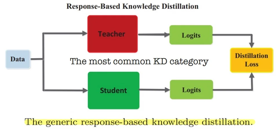
While response-based distillation is powerful, it assumes access to a pretrained and fixed teacher network—an assumption that breaks down in self-supervised learning, where no labeled data exists to train such a teacher. This motivates a natural question: can a model learn from itself in the absence of labels or external supervision?
Self-distillation (SD) emerges as a compelling answer. Rather than mimicking a separate teacher, the model supervises itself across different time steps or input views. This reframes knowledge distillation as an internal prediction alignment task and opens the door to label-free, contrastive-free representation learning.
We now explore the formulation and motivation behind self-distillation in greater depth.
From Classical KD to Self-Distillation Self-distillation (SD) adapts the teacher–student framework to the self-supervised setting, where no labels or pretrained teachers are available. Unlike classical knowledge distillation (KD), which transfers soft predictions from a fixed, pretrained teacher, SD involves a model teaching itself through the alignment of its own predictions across time and augmentations. This reframing introduces several core differences:
- Teacher origin: In KD, the teacher is a static, often overparameterized model trained with supervision. In SD, the teacher is a moving target: a slowly evolving exponential moving average (EMA) of the online model itself.
- Supervisory signal: KD aligns softmax distributions over classes. SD discards class supervision entirely and instead minimizes representation discrepancy across views—typically using cosine or MSE loss between learned embeddings.
- Training objective: KD is supervised or semi-supervised; SD is fully unsupervised and relies on view consistency for training.
Despite these differences, both paradigms are united by the use of soft targets—intermediate representations that provide a richer learning signal than hard labels alone. In SD, this soft signal comes not from external supervision, but from a stabilized, slowly moving reference.
Self-Distillation: Teacher-Free Prediction Alignment Self-distillation methods implement this paradigm via two networks with shared architecture:
- The online network, trained via backpropagation.
- The target network, updated via an EMA of the online network’s weights.
At each training step, the online network processes a view \( x^t \), while the target network encodes a separate view \( x^{t'} \) of the same image. A non-linear predictor head \( h \), applied only to the online network, introduces architectural asymmetry—a critical element for avoiding collapse. The loss is computed as:
\[ \mathcal {L}_{\mbox{SD}} = \left \| h(f_o(x^t)) - \mbox{stop_grad}(f_t(x^{t'})) \right \|^2, \]
where \( f_o \) and \( f_t \) are the encoders of the online and target networks, respectively. The stop_grad operator prevents gradients from flowing into the target branch, ensuring it provides a stable, fixed target.
Crucially, this loss operates on representation vectors—not logits—and does not require predefined classes. But this raises a conceptual puzzle: If both networks start from scratch, how does learning begin?
Cold Start and the Bootstrapping Feedback Loop A central puzzle in self-distillation is how training succeeds when both the online and target networks are randomly initialized. At first glance, the idea of learning from a ”teacher” that knows nothing appears paradoxical. Yet, in practice, self-distillation methods such as BYOL and SimSiam converge reliably. This success hinges on a carefully engineered interplay of asymmetries that enable the model to bootstrap its way to meaningful representations.
- Data asymmetry: Even with identical initial weights, the two branches receive different augmentations of the same input image. These distinct views lead to different encoder outputs, producing a nonzero initial loss and immediate gradients—providing a meaningful signal from the first step.
- Architectural asymmetry: A non-linear predictor head \( h \) is applied only to the online branch. This ensures that the network’s task is not merely to copy the target’s output, but to learn a transformation that aligns embeddings across different views. Without this asymmetry, collapse to trivial solutions (e.g., constant outputs) becomes a local minimum; with it, such solutions become unstable.
- Temporal asymmetry via EMA: The target network is updated as an exponential moving average (EMA) of the online network’s parameters. This produces a slowly evolving teacher that acts as a smoothed, temporally consistent guide. Early in training, even small improvements in the online network are gradually integrated into the target, allowing it to become a slightly better teacher over time.
Together, these asymmetries initiate a self-reinforcing learning loop: the online network improves slightly, the EMA target incorporates this improvement with stability, and the next iteration uses the improved target as a more informative reference. Over time, this dynamic leads to the emergence of increasingly structured representations.
But how can a model learn anything useful from an initially random target? The key insight is that learning does not require the target to be semantically meaningful from the start—it only needs to be consistent. Even a random network, when applied to different views of the same image, produces outputs with subtle statistical regularities.
By aligning its predictions to these weak but consistent signals, the online network begins to capture view-invariant structure. The EMA then amplifies and stabilizes this structure over time, enabling the system to progressively bootstrap richer representations from noise.
This bootstrapping mechanism—rooted in data diversity, architectural design, and temporal smoothing—explains how self-distillation avoids collapse and learns effectively from scratch, without labels or contrastive negatives.
Final Representation: What Do We Keep? A major trend across modern self-supervised learning (SSL) is the use of teacher–student architectures with distillation-like mechanisms. While not all methods—such as MoCo or SimCLR—fit the narrow definition of self-distillation, they adopt similar principles involving dual networks, embedding alignment, or moving-average targets. In these frameworks, the standard practice is to retain only the online encoder (backbone) after training, while discarding all auxiliary components.
- BYOL (self-distillation): “At the end of training, we only keep the encoder \( f_\theta \); everything else is discarded.”
- SimCLR (contrastive): “We throw away the projection head and use the encoder’s penultimate layer for downstream tasks.”
- DINO (self-distillation): “The features used in downstream tasks are the output of the backbone \( f \).”
- Barlow Twins (non-distillative): The projection head (called the expander) is discarded; only the encoder is retained.
This design choice is justified by both theoretical and practical considerations:
- The online encoder is the active learner. It is optimized via gradient descent and accumulates the learned representations by minimizing the self-supervised loss. Its parameters reflect the most up-to-date and discriminative features at the end of training.
- The target network is a training stabilizer. It acts as a slowly updated exponential moving average (EMA) of the online network. While it provides a stable signal throughout training, it is always lagging behind the online model. As such, it is not an independent model but an auxiliary ensembling mechanism.
- Auxiliary heads are task-specific. The predictor and projector are only necessary to shape the loss landscape during pretraining (e.g., for embedding alignment). They are not designed for general-purpose feature transfer, and often reduce information useful for downstream tasks [89, 194].
In summary, the encoder of the online network—the part trained to predict and adapt—captures the transferable structure learned during pretraining. The other components, though essential for enabling stable and effective training, are not retained. For downstream tasks, a new head (e.g., a linear classifier) is attached to the frozen or fine-tuned encoder. This separation between pretext optimization and transfer representation is central to the self-distillation pipeline.
Introduction Summary Self-distillation methods learn by enforcing consistency across views without contrastive loss or negative samples. Through architectural asymmetry, temporal smoothing, and internal bootstrapping, they extract rich representations from unlabeled data. This paradigm underlies modern frameworks such as BYOL, SimSiam, and DINO.
We now examine how these principles are instantiated, starting with BYOL’s use of a predictor head and momentum encoder to stabilize training.
22.4.3 Bootstrap Your Own Latent (BYOL)
Motivation: Learning Without Contrast Contrastive learning methods like SimCLR and MoCo rely heavily on negative pairs to prevent representational collapse. These methods require either extremely large batch sizes (e.g., 4096 in SimCLR) or auxiliary structures like momentum encoders and memory queues (as in MoCo). However, managing these negatives introduces several downsides: semantic repulsion, high GPU memory demand, sensitivity to augmentation strategies, and complex tuning of hyperparameters such as temperature.
In response to these limitations, BYOL [194] proposes a radically different approach: a self-distillation framework that learns meaningful representations without any form of negative samples. BYOL replaces the contrastive objective with a predictive one—minimizing the distance between two augmented views of the same image—enabled by a dual-network setup and architectural asymmetries that avoid collapse.
Architectural Overview Bootstrap Your Own Latent (BYOL) introduces a self-supervised framework built on two interacting neural networks: an online network, which is trained via gradient descent, and a target network, which provides stable targets without backpropagation. The two branches share the same backbone architecture but differ in their update mechanisms and structural components.
- Online Network (trainable): Composed of an encoder \( f_\theta \), a projector \( g_\theta \), and a predictor \( q_\theta \). The predictor head \( q_\theta \) is applied only in this branch and introduces essential asymmetry, playing a crucial role in preventing representational collapse.
- Target Network (non-trainable): Consists of an encoder \( f_\xi \) and a projector \( g_\xi \). Its parameters are updated using an exponential moving average (EMA) of the online network’s weights: \[ \xi \leftarrow \tau \xi + (1 - \tau ) \theta \] where \( \tau \in [0, 1) \) is a momentum coefficient, typically initialized at \( \tau = 0.996 \) and gradually increased to 1.
For each image \( x \), BYOL applies two stochastic data augmentations, producing two distinct views \( v = t(x) \) and \( v' = t'(x) \). The online network processes \( v \) through its encoder–projector–predictor pipeline to yield a predicted representation. Simultaneously, the target network processes \( v' \) through its encoder and projector to generate a target embedding. The objective is to align these outputs without requiring negative examples.
Mathematical Formulation and Training Objective Let \( x \in \mathcal {D} \) be an input image. BYOL applies two independent stochastic augmentations to obtain views \( v = t(x) \) and \( v' = t'(x) \). These views are processed by two networks:
- Online network (learned via backpropagation): composed of an encoder \( f_\theta \), a projection head \( g_\theta \), and a predictor head \( q_\theta \). It computes: \[ y_\theta = f_\theta (v), \quad z_\theta = g_\theta (y_\theta ), \quad p_\theta = q_\theta (z_\theta ) \]
- Target network (updated via EMA): composed of encoder \( f_\xi \) and projector \( g_\xi \), with: \[ y'_\xi = f_\xi (v'), \quad z'_\xi = g_\xi (y'_\xi ) \]
To ensure stable training, both outputs are \( \ell _2 \)-normalized: \[ \bar {p}_\theta = \frac {p_\theta }{\|p_\theta \|_2}, \quad \bar {z}'_\xi = \frac {z'_\xi }{\|z'_\xi \|_2} \]
The core objective encourages the online prediction \( \bar {p}_\theta \) to align with the target projection \( \bar {z}'_\xi \), treated as a constant using a stop-gradient operator: \[ \mathcal {L}_{\theta ,\xi }(v, v') = \left \| \bar {p}_\theta - \texttt{sg}(\bar {z}'_\xi ) \right \|_2^2 \] This squared \( \ell _2 \)-distance is equivalent to maximizing cosine similarity between unit vectors. The stop-gradient (sg) operator halts gradient flow through the target branch, enforcing an optimization asymmetry that is crucial for collapse prevention.
To ensure balanced learning and prevent the network from specializing in predicting only one view from the other, BYOL symmetrizes the loss by swapping the roles of the online and target branches across augmentations. Specifically, the second augmented view \( v' \) is passed through the online network and the first view \( v \) through the target network, producing a second prediction–target pair: \[ \tilde {\mathcal {L}}_{\theta ,\xi }(v', v) = \left \| \bar {p}_\theta ' - \texttt{sg}(\bar {z}_\xi ) \right \|_2^2 \] where \( \bar {p}_\theta ' = q_\theta (g_\theta (f_\theta (v'))) \) and \( \bar {z}_\xi = \frac {g_\xi (f_\xi (v))}{\|g_\xi (f_\xi (v))\|_2} \). This symmetry ensures that both augmentations contribute equally to representation learning and mitigates potential bias arising from fixed network roles.
The final training objective combines both directions: \[ \mathcal {L}_{\mbox{BYOL}} = \mathcal {L}_{\theta ,\xi }(v, v') + \tilde {\mathcal {L}}_{\theta ,\xi }(v', v) \]
Unlike contrastive frameworks that depend on repulsion between negatives, BYOL relies solely on positive pair alignment. Its ability to avoid collapse stems not from the loss formulation alone, but from a carefully balanced design: the predictor head introduces architectural asymmetry, the EMA target stabilizes learning trajectories, and the stop-gradient mechanism prevents trivial feedback loops. Together, these elements enable the model to distill invariant, semantically meaningful features from raw, unlabelled data. We’ll uncover it in detail later.
Robustness and Empirical Performance A central strength of BYOL lies in its robustness to design constraints that affect contrastive methods. Unlike SimCLR, which degrades significantly without large batch sizes or aggressive data augmentations, BYOL maintains high performance under less demanding setups.
Batch Size Robustness. BYOL does not depend on negative sampling, and thus avoids the batch size bottleneck inherent in contrastive methods. While SimCLR relies on large batches (e.g., 4096) to yield diverse negatives, BYOL performs well down to a batch size of 256. Below 128, performance does decline—but this is attributed to the batch normalization statistics becoming unreliable at small batch sizes, rather than any flaw in BYOL’s learning dynamics.
Augmentation Robustness. SimCLR’s reliance on strong augmentations (e.g., color jitter, grayscale) is tied to its need to create hard positives and diverse negatives. In contrast, BYOL learns by aligning predictions, not discriminating between pairs, and therefore suffers less when specific augmentations are removed. While strong augmentations still help, BYOL’s learning signal is less fragile, making it easier to deploy in practice with simplified data pipelines.
Linear Evaluation on ImageNet To assess representational quality, BYOL is evaluated using the standard linear probing protocol on ImageNet: the encoder is frozen and a linear classifier is trained on top. BYOL sets a new state of the art across several architectures.
Semi-Supervised Evaluation BYOL also excels in label-scarce regimes. When trained with just 1% or 10% of labeled ImageNet data, it significantly outperforms prior work.
Transfer to Downstream Tasks Pretraining with BYOL produces highly transferable representations. On 12 downstream datasets evaluated under linear probing, BYOL outperforms both SimCLR and supervised ImageNet baselines in most cases.
| Method | Food101 | CIFAR10 | CIFAR100 | Birdsnap | SUN397 | Cars | Aircraft | VOC07 | DTD | Pets | Caltech101 | Flowers |
| BYOL (ours) | 75.3 | 91.3 | 78.4 | 57.2 | 62.2 | 67.8 | 60.6 | 82.5 | 75.5 | 90.4 | 94.2 | 96.1 |
| SimCLR [89] | 72.8 | 90.5 | 74.4 | 42.4 | 60.6 | 49.3 | 49.8 | 81.4 | 75.7 | 84.6 | 89.3 | 92.6 |
| Supervised-IN | 72.3 | 93.6 | 78.3 | 53.7 | 61.9 | 66.7 | 61.0 | 82.8 | 74.9 | 91.5 | 94.5 | 94.7 |
Ablation Studies and Collapse Prevention Extensive ablation studies reveal that BYOL’s success hinges on a triad of mechanisms designed to destabilize trivial solutions and guide the optimizer toward informative representations:
- Predictor \( q_\theta \): A non-linear MLP head applied only to the online branch. Its architectural asymmetry is critical: without it, the online encoder can trivially match the target’s output, resulting in representational collapse. This is empirically confirmed by the original BYOL ablation, where removing the predictor yields just 0.2% top-1 accuracy [194], and reinforced by later works like SimSiam, in which the authors observed that the predictor stabilizes training even without a momentum encoder [93].
- EMA Target Update (\( \tau \)): The target network is updated as an exponential moving average of the online parameters. Setting \( \tau = 0 \) eliminates temporal smoothing, effectively collapsing the two branches and destabilizing learning. Conversely, fixing \( \tau = 1 \) stalls the target, preventing progressive refinement. BYOL operates best under a high-momentum regime (e.g., \( \tau \approx 0.996 \)), which introduces a slow-evolving supervisory signal [194, 636].
- Stop-Gradient: Gradients are prevented from flowing into the target branch, breaking symmetry and avoiding trivial co-adaptation. Without this operation, the encoder and predictor can conspire to output constant vectors that yield low loss, leading to collapse [93].
Each of BYOL’s core mechanisms—predictor asymmetry, EMA target updates, and stop-gradient, addresses a distinct failure mode that could otherwise lead to representational collapse. While a constant-output encoder can technically minimize the loss, this solution becomes unstable under BYOL’s training dynamics. In particular, the online network is constantly updated to match a target that is slowly changing and view-dependent. Attempting to align all predictions to a fixed, uninformative vector becomes increasingly inconsistent and error-prone as training progresses. This makes the trivial solution difficult for the optimizer to maintain.
A useful analogy is that of a pencil balanced on its tip: although this is a valid equilibrium in theory, it is so sensitive to perturbations that it cannot be maintained in practice. Likewise, in BYOL, the combination of architectural asymmetry and temporal smoothing renders the collapsed solution highly sensitive to random fluctuations and gradient noise. As a result, optimization is naturally repelled away from collapse and drawn toward more stable solutions—namely, feature-rich representations that reflect consistent structure across augmented views [636].
Recent theoretical analyses reinforce this intuition. Although a degenerate, constant-output solution can trivially minimize the BYOL loss, such a solution is structurally fragile. The predictor must map diverse augmentations to a fixed target representation—an unrealistic objective if the features encode no meaningful variation. Instead, BYOL implicitly promotes alignment of principal components across views and disperses variance across feature dimensions [636, 774]. These emergent properties parallel the explicit redundancy-reduction objectives introduced later in VICReg and Barlow Twins.
Finally, standard deep learning practices further bolster training stability. Random initialization ensures that optimization begins in a diverse regime, away from degenerate attractors. Batch Normalization injects stochasticity and enforces re-centering, making it harder for the model to converge to constant outputs. While neither mechanism alone is sufficient to prevent collapse—and BYOL has been shown to function even without batch statistics [545]—their inclusion supports better optimization and generalization throughout training.
Conclusion BYOL marked a turning point in self-supervised learning by showing that predictive alignment—without contrastive negatives—can produce strong, transferable representations. Its stability arises not from the loss itself, but from three key mechanisms: a predictor for architectural asymmetry, EMA for temporal smoothing, and stop-gradient for optimization decoupling. Together, they prevent collapse and promote invariant feature learning.
This success prompts a natural question: Can these benefits be retained without the EMA target? SimSiam explores this possibility by preserving the predictor and stop-gradient, but removing the momentum encoder. We now examine its simplified design and theoretical insights.
22.4.4 SimSiam: Self-Supervised Learning Without Negative Pairs or Momentum
Motivation: Can Collapse Be Avoided Without Negatives or EMA? SimSiam [93] explores a surprising and insightful question at the heart of self-supervised representation learning: Can we avoid collapse without contrastive negatives or a momentum-updated target network? Building on architectural insights from BYOL [194], SimSiam introduces a drastically simplified framework that removes both of these components—long believed to be essential for training stability—and retains only one asymmetry: the stop-gradient operation.
The framework employs a Siamese setup, where two augmented views of the same image are processed through identical encoders. Crucially, the gradient is only allowed to flow through one branch, while the other is treated as a fixed target. This seemingly minimal intervention proves sufficient to prevent representational collapse. Empirically, SimSiam achieves competitive performance among non-contrastive methods, despite its conceptual simplicity and lack of auxiliary targets or negative sampling.
Although SimSiam does not reach state-of-the-art accuracy, it plays a pivotal role in understanding why self-distillation methods work and which mechanisms are truly necessary for stable learning. It reveals that collapse prevention can emerge purely from gradient-level asymmetry, while other components—such as momentum encoders or batch normalization—may be helpful but not essential. As such, SimSiam is not merely a practical method but a crucial analytical probe into the foundations of self-supervised learning.
Architecture and Symmetric Learning Mechanism SimSiam employs a symmetric Siamese architecture to compare two augmented views of a single image. Given an input \( x \), two views \( x_1 = t(x) \) and \( x_2 = t'(x) \) are generated through independent data augmentations. These views are processed by a shared-weight network composed of:
- Encoder \( f(\cdot ) \): a shared backbone (typically ResNet-50) followed by a projection MLP. The encoder maps each augmented view to a projected representation \( z \).
- Prediction head \( h(\cdot ) \): an MLP applied only to one branch to break symmetry and introduce gradient asymmetry.
Let the intermediate representations be: \[ z_1 = f(x_1), \quad z_2 = f(x_2), \quad p_1 = h(z_1), \quad p_2 = h(z_2) \]
SimSiam minimizes the negative cosine similarity between predictions and the stop-gradient-protected projections of the other view: \[ \mathcal {D}(p_1, z_2) = - \frac {p_1}{\|p_1\|_2} \cdot \frac {z_2}{\|z_2\|_2}, \quad \mathcal {D}(p_2, z_1) = - \frac {p_2}{\|p_2\|_2} \cdot \frac {z_1}{\|z_1\|_2} \]
To avoid biasing the learning toward one view, SimSiam symmetrizes the loss by swapping the roles of the two views and aggregating both prediction-target pairs. The final training objective is: \[ \mathcal {L}_{\mbox{SimSiam}} = \frac {1}{2} \mathcal {D}(p_1, \texttt{sg}(z_2)) + \frac {1}{2} \mathcal {D}(p_2, \texttt{sg}(z_1)) \]
Here, \( \texttt{sg}(\cdot ) \) denotes the stop-gradient operation, which halts gradient flow through the target branch.
SimSiam Training Pseudocode The following pseudocode illustrates SimSiam’s core training loop. It highlights the minimalist design that enables stable representation learning without contrastive pairs or a target network. The encoder \( f \) (composed of a backbone and a projection MLP) processes two augmented views \( x_1 \) and \( x_2 \) of each input image. The prediction MLP \( h \) is then applied to each projection, and the loss is computed as the average negative cosine similarity between cross-view prediction–target pairs. Crucially, the function D includes a detach() operation on \( z \), implementing the stop-gradient mechanism that prevents representational collapse by freezing the target features during backpropagation.
# f: backbone + projection mlp
# h: prediction mlp

for x in loader:  # load a minibatch x with n samples
    x1, x2 = aug(x), aug(x)  # random augmentation
    z1, z2 = f(x1), f(x2)    # projections, n-by-d
    p1, p2 = h(z1), h(z2)    # predictions, n-by-d

    L = D(p1, z2)/2 + D(p2, z1)/2  # loss

    L.backward()     # back-propagate
    update(f, h)     # SGD update


def D(p, z):  # negative cosine similarity
    z = z.detach()  # stop gradient
    p = normalize(p, dim=1)  # l2-normalize
    z = normalize(z, dim=1)  # l2-normalize
    return -(p * z).sum(dim=1).mean()
Gradient Formula and Learning Signal SimSiam’s training objective is defined by a symmetrized negative cosine similarity loss: \[ \mathcal {L}_{\mbox{SimSiam}} = \frac {1}{2} \mathcal {D}(p_1, \texttt{sg}(z_2)) + \frac {1}{2} \mathcal {D}(p_2, \texttt{sg}(z_1)) \] where \( p_1 = h(f(x_1)) \), \( z_2 = f(x_2) \), and \[ \mathcal {D}(p, z) = - \frac {p}{\|p\|_2} \cdot \frac {z}{\|z\|_2} \] is the negative cosine similarity between \(\ell _2\)-normalized vectors.
Focusing on the first term, \( \mathcal {L}_1 = \frac {1}{2} \mathcal {D}(p_1, \texttt{sg}(z_2)) \), the stop-gradient operator ensures that \( z_2 \) is treated as a constant during backpropagation. Thus, gradients flow only through the predicting branch.
Let \( P_1 = p_1 / \|p_1\|_2 \) and \( Z_2 = z_2 / \|z_2\|_2 \), so that: \[ \mathcal {L}_1 = -\frac {1}{2} P_1 \cdot Z_2 \] Since \( Z_2 \) is fixed, the gradient with respect to \( p_1 \) is given by: \[ \frac {\partial \mathcal {L}_1}{\partial p_1} = -\frac {1}{2} \cdot \frac {\partial P_1}{\partial p_1}^\top Z_2 \] Using the identity: \[ \frac {\partial P_1}{\partial p_1} = \frac {1}{\|p_1\|_2} \left ( I - \frac {p_1 p_1^\top }{\|p_1\|_2^2} \right ) \] we obtain the explicit gradient: \[ \frac {\partial \mathcal {L}_1}{\partial p_1} = -\frac {1}{2} \left ( \frac {z_2}{\|p_1\|_2 \|z_2\|_2} - \frac {(p_1 \cdot z_2) p_1}{\|p_1\|_2^3 \|z_2\|_2} \right ) \] This learning signal pulls \( p_1 \) toward alignment with the fixed \( z_2 \), encouraging consistent representations across augmentations.
Gradients are then propagated backward through the prediction head \( h \) and encoder \( f \) via the chain rule: \[ \frac {\partial \mathcal {L}_1}{\partial \theta _h} = \frac {\partial \mathcal {L}_1}{\partial p_1} \cdot \frac {\partial p_1}{\partial \theta _h}, \qquad \frac {\partial \mathcal {L}_1}{\partial \theta _f} = \frac {\partial \mathcal {L}_1}{\partial p_1} \cdot \frac {\partial p_1}{\partial z_1} \cdot \frac {\partial z_1}{\partial \theta _f} \] This selective update mechanism enforces asymmetry: only the predicting branch is optimized in each term, while the target remains a fixed reference.
The stop-gradient operation acts as a structural constraint that prevents representational collapse. Without it, gradients flow symmetrically through both branches, allowing the shared encoder \( f \) to trivially minimize the loss by collapsing all outputs to a constant vector \( c \). If all outputs align perfectly, then: \[ p_1 = z_2 = p_2 = z_1 = c \quad \Rightarrow \quad \frac {p}{\|p\|_2} = \frac {z}{\|z\|_2} \quad \Rightarrow \quad \mathcal {D}(p, z) = -1 \] Since the SimSiam objective is symmetrized and each term is weighted by \( \frac {1}{2} \), the total loss becomes: \[ \mathcal {L}_{\mbox{SimSiam}} = \frac {1}{2}(-1) + \frac {1}{2}(-1) = -1 \] This value represents the global minimum of the objective. However, it corresponds to a degenerate solution in which all representations collapse to a single direction on the unit sphere. In this state, feature variance across the batch approaches zero, and the learned representations become uninformative for downstream tasks.
The stop-gradient prevents this collapse by halting gradient flow into one branch—treating its representation as a fixed learning target. This breaks the co-adaptation loop that would otherwise allow the model to coordinate both views toward trivial agreement. Instead, the predicting branch (through \( h \) and \( f \)) must learn to match a (hopefully) non-trivially evolving target \( z \), whose variability is preserved by being exempt from gradient updates in that loss term. Empirically, SimSiam without stop-gradient rapidly converges to this trivial solution with a loss of \( -1 \), near-zero standard deviation in outputs, and chance-level accuracy [93]. In contrast, with stop-gradient, the network is compelled to extract meaningful, invariant features across augmentations, sustaining both representation quality and diversity.
EM-Like Interpretation of SimSiam Training SimSiam’s optimization can be interpreted as an online, alternating process analogous to the Expectation-Maximization (EM) algorithm. This perspective helps explain how SimSiam avoids collapse despite its symmetric architecture and lack of contrastive negatives or momentum encoders.
Let \( \eta _x \) denote a latent target representation for image \( x \). SimSiam implicitly minimizes the following population objective: \[ \mathcal {L}(\theta , \eta ) = \mathbb {E}_{x,\,T} \left [ \| f_\theta (T(x)) - \eta _x \|_2^2 \right ] \] where \( f_\theta \) is the encoder (including the projection MLP), \( \eta _x \) is an instance-specific latent representation, and \( T \sim \mathcal {T} \) denotes a random data augmentation sampled from the augmentation distribution \( \mathcal {T} \).
Optimizing both \( \theta \) and \( \eta \) jointly would lead to degenerate solutions. Instead, SimSiam implicitly performs the following alternating procedure at each iteration:
- E-step (Target estimation): Fix \( \theta \), and approximate \( \eta _x \leftarrow f_\theta (T'(x)) \), where \( T'(x) \sim \mathcal {T} \) is a fresh stochastic augmentation. In practice, this corresponds to computing the second view’s representation \( z_2 = f(x_2) \) and freezing it via the stop-gradient operator: \( \eta _x = \texttt{sg}(z_2) \).
- M-step (Parameter update): Fix \( \eta _x \), and update \( \theta \) to minimize \( \| f_\theta (T(x)) - \eta _x \|_2^2 \). This corresponds to computing \( p_1 = h(f(x_1)) \), and updating the parameters of \( f \) and \( h \) to align the prediction with the frozen target \( z_2 \).
This alternating behavior is what prevents collapse. The target \( \eta _x \) varies stochastically due to different augmentations drawn from \( \mathcal {T} \), which include cropping, color jittering, flipping, and blurring. Consequently, the model isn’t likely to simply map every input to a constant vector. Instead, it’s encouraged to learn how to produce a representation \( f(x_1) \) that generalizes across augmentations and can be transformed by the predictor \( h \) into an accurate match for \( z_2 \).
The presence of the prediction head \( h \) further supports this EM interpretation. Since the E-step is approximated using a single sample rather than the expectation \( \mathbb {E}_T[f(T(x))] \), \( h \) learns to compensate for this variability, acting as a regression head that bridges the gap between stochastic projections. Empirically, removing or fixing \( h \) causes the model to collapse, reinforcing its role in stabilizing the alternating optimization.
In summary, SimSiam’s use of stop-gradient transforms a structurally symmetric architecture into an asymmetrically optimized system. This EM-like view provides a principled justification for the training dynamics, explaining how the model achieves non-trivial representation learning without explicit negative samples or temporal ensembling.
Conclusion: Stop-Gradient as a Structural Inductive Bias This asymmetric optimization induced by the stop-gradient operation is not merely a stabilizing detail—it is the cornerstone of SimSiam’s ability to extract useful representations from unlabeled data. It reshapes the training dynamics in a way that not only avoids trivial solutions, but also encourages robustness to augmentation, separation of semantics, and sensitivity to structure.
But how critical is this mechanism in practice? To what extent do other components—such as the prediction head, batch normalization, or network depth—contribute to the method’s success? The following part delves into SimSiam’s empirical landscape, dissecting its architecture through targeted ablations and revealing which ingredients are essential for stability, performance, and generalization.
Empirical Validation of the Stop-Gradient Mechanism SimSiam’s most critical empirical finding is that the stop-gradient operation is indispensable for preventing representational collapse. When the stop-gradient is removed, the network degenerates immediately, producing near-constant outputs and achieving no meaningful accuracy—even on simple benchmarks. This collapse is evidenced by three distinct indicators:
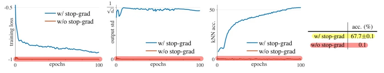
- Loss dynamics: Without stop-gradient, the training loss plummets to a trivial minimum, reflecting degenerate convergence.
- Representation collapse: The standard deviation across channels drops sharply, indicating that all output vectors are collapsing to a single mode.
- kNN classification: Downstream utility is destroyed—accuracies approach random guess levels.
These findings confirm that the stop-gradient is not merely a training trick—it is the primary stabilizing force in SimSiam. By freezing one side of the network, the method introduces a hard asymmetry that prevents both branches from co-adapting to trivial solutions. It also reduces mutual drift, anchoring learning around a fixed target.
Ablation Studies and Analysis To better understand the mechanisms underlying SimSiam’s stability and performance, the authors conduct a series of ablation studies [93]. These experiments systematically isolate the role of the prediction head, learning rate decay, batch size, and BatchNorm placement. The results reinforce that while many design choices improve training dynamics, only a few are truly critical for preventing collapse.
| Variation | Accuracy (%) |
|---|---|
| Baseline (predictor MLP + lr decay) | 67.7 |
| (a) No predictor MLP | 0.1 |
| (b) Fixed random predictor | 1.5 |
| (c) No learning rate decay | 68.1 |
The predictor MLP \( h \) is indispensable. When removed or fixed, the system collapses to degenerate solutions. This highlights that \( h \) not only introduces a necessary asymmetry but must remain trainable to track the evolving representations. Moreover, disabling learning rate decay on \( h \) improves results—likely because \( h \) must continuously adapt to non-stationary targets \( z_2 \), a behavior consistent with the EM-like interpretation of SimSiam’s training dynamics.
| Batch Size | 64 | 128 | 256 | 512 | 1024 | 2048 | 4096 |
|---|---|---|---|---|---|---|---|
| Accuracy (%) | 66.1 | 67.3 | 68.1 | 68.1 | 68.0 | 67.9 | 64.0 |
SimSiam achieves strong results even at small batch sizes, in contrast to contrastive methods like SimCLR that require large batches to construct effective negative sets. At extreme batch sizes (e.g., 4096), performance drops slightly—not because of collapse, but due to reduced stochasticity in BatchNorm and diminished gradient noise. This mirrors similar limitations observed in supervised training with large batches. Optimizers like LARS could potentially mitigate this, though they are not required for stability.
| Case | Proj. BN | Pred. BN (output) | Accuracy (%) |
|---|---|---|---|
| (a) No BN | – | – | 34.6 |
| (b) Hidden-only BN | ✓ | – | 67.4 |
| (c) Default (hidden+output) | ✓ | – | 68.1 |
| (d) All BN (incl. pred. output) | ✓ | ✓ | unstable |
BatchNorm is beneficial when applied to the hidden layers of the projection and prediction MLPs, where it improves convergence by reducing internal covariate shift and smoothing the loss landscape. This effect is evident in cases (b) and (c), which significantly outperform the no-BN baseline (a).
However, applying BN to the final output of the prediction MLP—as in case (d)—causes the model to diverge. This is not due to collapse (i.e., the model outputting a constant vector), but rather to optimization instability: the loss becomes erratic, and training fails to converge. The root cause is a conflict between BatchNorm’s standardization objective and the alignment objective of the cosine similarity loss.
To illustrate: the cosine similarity loss encourages the predicted vector \( p_1 \) to point in the same direction as the stop-gradient target \( z_2 \). But BatchNorm normalizes each output dimension across the batch to zero mean and unit variance, thereby erasing consistent directional signals that span the batch. For example, if a feature dimension consistently activates for a particular semantic concept (e.g., ”dog” images), BatchNorm will force this signal back toward zero, undermining the model’s effort to align \( p_1 \) and \( z_2 \). As a result, the loss and the normalization act at cross-purposes, producing gradients that oscillate and fail to descend smoothly.
This instability is a distinct failure mode: while the model does not collapse, it also cannot learn. Therefore, the lesson is not merely to use BN, but to use it strategically: allow it to regularize internal representations, but avoid placing it at points where it interferes with critical geometric constraints like those enforced by cosine similarity.
In summary, SimSiam’s ablation studies reveal a delicate interplay between network architecture and training dynamics. Preventing collapse depends not only on the presence of the stop-gradient and a learnable prediction head, but also on ensuring that optimization components like BatchNorm cooperate with—rather than counteract—the training objective.
Comparison to Other Self-Supervised Methods SimSiam’s performance is benchmarked against leading methods including SimCLR, MoCo v2, BYOL, and SwAV. Remarkably, SimSiam achieves comparable performance despite being simpler and not requiring negative samples, large batches, or momentum encoders.
| Method | Neg. Pairs | Momentum | 100 ep | 800 ep |
|---|---|---|---|---|
| SimCLR (repro.) | ✓ | – | 66.5 | 70.4 |
| MoCo v2 (repro.) | ✓ | ✓ | 67.4 | 72.2 |
| BYOL (repro.) | – | ✓ | 66.5 | 74.3 |
| SwAV (repro.) | – | – | 66.5 | 71.8 |
| SimSiam | – | – | 68.1 | 71.3 |
| Method | VOC07 AP | VOC07+12 AP | COCO Det. AP | COCO Seg. AP |
|---|---|---|---|---|
| ImageNet Sup. | 42.4 | 53.5 | 38.2 | 33.3 |
| SimCLR (repro.) | 46.8 | 55.5 | 37.9 | 33.3 |
| MoCo v2 (repro.) | 48.5 | 57.0 | 39.2 | 34.3 |
| BYOL (repro.) | 47.0 | 55.3 | 37.9 | 33.2 |
| SwAV (repro.) | 46.5 | 55.4 | 37.6 | 33.1 |
| SimSiam (base) | 47.0 | 56.4 | 37.9 | 33.2 |
| SimSiam (opt.) | 48.5 | 57.0 | 39.2 | 34.4 |
Paper Summary SimSiam’s primary contribution lies in its radical simplification of self-supervised learning. By eliminating the need for negative pairs and momentum encoders, it reveals that the stop-gradient operation alone—when paired with architectural asymmetry and prediction—can stabilize training and prevent collapse. This simplicity does not come at the cost of performance: SimSiam rivals more complex frameworks on standard benchmarks, and its ablations underscore the critical role of its asymmetries in training dynamics.
SimSiam’s findings challenge earlier assumptions from contrastive learning and BYOL: namely, that collapse prevention demands external mechanisms such as queues or target encoders. Instead, SimSiam highlights the importance of gradient flow structure rather than network complexity. Its implicit EM-like interpretation and empirical robustness invite new design patterns in self-supervised learning that prioritize architectural asymmetry and prediction dynamics.
This shift sets the stage for the emergence of methods like DINO, which further extend these ideas in several directions:
- From instance-level to token-level supervision: While SimSiam aggregates representations over the entire image, DINO introduces finer-grained self-distillation using ViT tokens, allowing localized learning signals.
- From representation alignment to cluster emergence: SimSiam optimizes similarity losses between two views. DINO, by contrast, encourages the emergence of semantically meaningful clusters—without requiring labels.
- From architectural asymmetry to output sharpening: DINO stabilizes training not only through stop-gradients and momentum encoders, but also by temperature sharpening and centering of the output logits—mechanisms that expand and refine the core idea of bootstrapping.
In the following subsection, we explore DINO (Self-Distillation with No Labels) [70], a milestone that blends SimSiam’s SG asymmetry, BYOL’s EMA targets, and transformer-specific innovations to enable the emergence of semantic structure in vision transformers—without supervision.
22.4.5 DINO: Self-Distillation with No Labels
Motivation: From Invariance to Semantic Understanding Self-supervised learning (SSL) has steadily progressed from contrastive methods such as SimCLR [89] and MoCo [220] to non-contrastive approaches like BYOL [194] and SimSiam [93]. Each iteration has reduced reliance on negative pairs or auxiliary targets. DINO [70] marks a conceptual leap by combining self-distillation with Vision Transformers (ViTs) [134], enabling strong visual representations—and even emergent semantic segmentation—without supervision.
The motivation behind DINO is twofold. First, the authors seek to exploit the inductive capacity of ViTs without the constraints of predefined labels. Second, they aim to go beyond learning invariances to augmentations—toward improved semantic understanding. Remarkably, DINO-trained ViTs learn to identify object boundaries and semantic regions using only internal attention, with no labels provided during training.
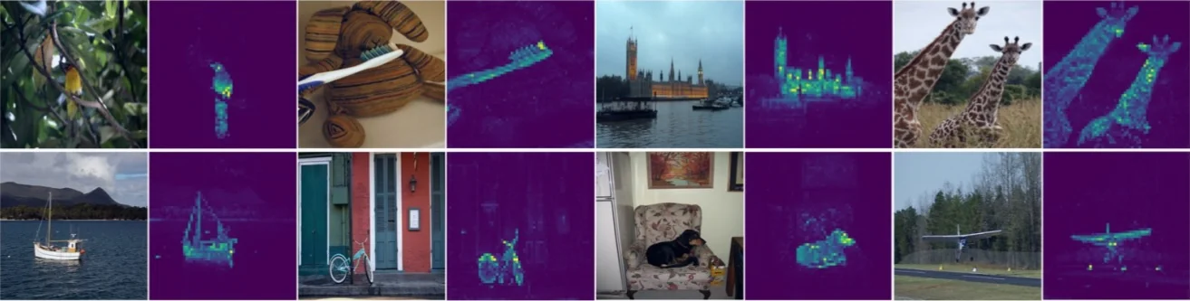
Self-Distillation Without Labels DINO—short for DIstillation with NO labels—frames self-supervised learning as a teacher–student distillation task without any labeled data. Both the student \( g_{\theta _s} \) and teacher \( g_{\theta _t} \) networks share the same architecture (typically a ViT backbone followed by an MLP head), but differ in how their parameters evolve:
- The student network \( g_{\theta _s} \) is updated via standard backpropagation.
- The teacher network \( g_{\theta _t} \) is updated as an exponential moving average (EMA) of the student: \[ \theta _t \leftarrow \lambda \theta _t + (1 - \lambda ) \theta _s \] where \( \lambda \in [0.996, 1.0] \) controls the EMA momentum.
This EMA update, inherited from BYOL, ensures that the teacher changes slowly over time, providing stable and high-quality training targets. Throughout training, the teacher consistently produces better representations than the student, guiding it toward semantically meaningful features.
Multi-Crop Strategy and View Asymmetry DINO formulates self-supervised learning as a knowledge distillation task between a student network \( g_{\theta _s} \) and a teacher network \( g_{\theta _t} \), parameterized by \( \theta _s \) and \( \theta _t \), respectively. Both networks share the same architecture, but only the student is updated via gradient descent. The teacher parameters are updated using an exponential moving average (EMA) of the student parameters.
From each input image, DINO samples a set of augmented views \( V \) using a multi-crop strategy:
- Two global views \( x_1^g, x_2^g \in V \), high-resolution crops (e.g., \( 224 \times 224 \)) that each cover a large portion of the image.
- Several local views \( x' \in V \setminus \{x_1^g, x_2^g\} \), smaller crops (e.g., \( 96 \times 96 \)) that focus on limited regions.
The student network \( g_{\theta _s} \) processes all views \( x' \in V \), while the teacher network \( g_{\theta _t} \) processes only the global views \( x \in \{x_1^g, x_2^g\} \). This asymmetry enforces a local-to-global learning objective, where the student must produce predictions from partial information (local crops) that are consistent with the teacher’s output on broader contextual views (global crops).
Each network outputs a \( K \)-dimensional vector that is interpreted as unnormalized logits over \( K \) output bins. These logits are then normalized into a categorical probability distribution using a temperature-scaled softmax. For the student network, the output distribution is defined as: \begin {equation} P_s(x')^{(i)} = \frac {\exp (g_{\theta _s}(x')^{(i)} / \tau _s)}{\sum _{k=1}^{K} \exp (g_{\theta _s}(x')^{(k)} / \tau _s)}, \end {equation} where \( P_s(x')^{(i)} \) denotes the normalized probability assigned to the \( i \)-th output dimension, and \( \tau _s > 0 \) is the temperature parameter controlling the entropy of the student distribution: larger \( \tau _s \) produces softer (higher-entropy) outputs.
For the teacher network, the output distribution is computed similarly, but includes a centering term and a lower temperature for sharpening: \begin {equation} P_t(x)^{(i)} = \frac {\exp ((g_{\theta _t}(x)^{(i)} - C^{(i)}) / \tau _t)}{\sum _{k=1}^{K} \exp ((g_{\theta _t}(x)^{(k)} - C^{(k)}) / \tau _t)}, \end {equation} where \( \tau _t \ll \tau _s \) induces sharper, more peaked teacher predictions, and the centering vector \( C \in \mathbb {R}^K \) is updated via exponential moving average of the teacher outputs over the batch. The purpose of centering is to prevent collapse to a trivial solution in which one output bin dominates across all images and views. Together, centering and sharpening ensure that the teacher provides a stable, informative target distribution.
The training objective is to align the student’s prediction on one view \( x' \in V \) with the teacher’s prediction on a different view \( x \in \{x_1^g, x_2^g\} \), where \( x' \ne x \). This promotes consistency across differently sized or positioned crops from the same image, enabling the student to learn invariant semantic representations. The objective minimizes the cross-entropy between teacher and student outputs: \begin {equation} \min _{\theta _s} \sum _{x \in \{x_1^g, x_2^g\}} \sum _{\substack {x' \in V \\ x' \ne x}} H\big ( \texttt{sg}(P_t(x)),\, P_s(x') \big ), \end {equation} where the cross-entropy is defined as \( H(p, q) = -\sum _{i=1}^K p^{(i)} \log q^{(i)} \), and \( \texttt{sg}(\cdot ) \) denotes the stop-gradient operator applied to the teacher’s output to prevent gradients from flowing into \( g_{\theta _t} \). Only the student parameters \( \theta _s \) are updated via backpropagation, while the teacher parameters \( \theta _t \) are updated via EMA.
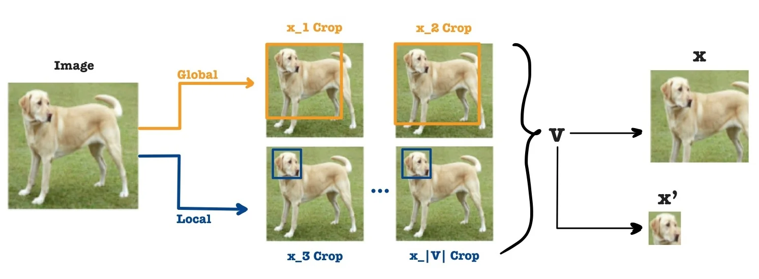
This asymmetric design—across view assignment, parameter updates, and output normalization—is central to DINO’s ability to learn structured representations without collapse. The use of multi-crop views, particularly the contrast between local and global crops, forces the student to infer the teacher’s global semantic predictions from partial observations. This promotes object-centric representations, robustness to occlusion, and invariance to viewpoint and scale—all without requiring negative pairs or a prediction head.
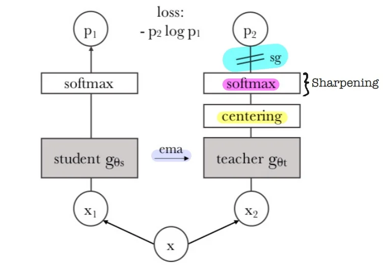
Architectural Backbone: Why Vision Transformers? Vision Transformers (ViTs) are particularly well-suited to DINO’s self-distillation framework. As introduced in Section §18, ViTs tokenize an input image into fixed-size patches, which are embedded and processed via stacked self-attention layers. A special learnable token—[CLS]—is prepended to the patch sequence and serves as a global aggregator. Its final representation is typically used as the image-level summary.
In DINO, the output of the [CLS] token is passed through a projection head: a 3-layer MLP that transforms the \( D \)-dimensional backbone output into a \( K \)-dimensional logit vector. These logits represent the model’s assignment over \( K \) emergent prototypes or semantic bins and serve as the input to the softmax used in the self-distillation loss. Thus, while the [CLS] token itself captures holistic image semantics, it is the post-MLP logits—derived from it—that define the probabilistic targets and predictions compared between the teacher and student.
This architectural separation is crucial: the ViT backbone focuses on learning rich, position-aware image features via attention, while the projection head maps the globally pooled [CLS] embedding into a space amenable to self-supervised alignment. The student is trained to match the teacher’s softened and centered output distributions over these prototypes, even from smaller local crops. This interaction—between ViT’s global summarization, DINO’s multi-view setup, and the projection into a high-rank prototype space—is what enables strong, semantically aligned features to emerge without supervision.
In the following parts, we formalize the training algorithm via pseudocode and dissect the core components of DINO’s loss—centering, sharpening, and their interplay with temperature scaling.
Preventing Collapse with Centering and Sharpening A central challenge in self-supervised learning is avoiding representational collapse—a degenerate regime in which the model produces trivial or uninformative outputs. This pathology arises when the training objective admits solutions that minimize the loss without learning useful representations. DINO avoids collapse not through architectural asymmetry—such as a prediction head used in BYOL [194] or SimSiam [93]—but through a carefully constructed functional asymmetry, applied only to the teacher network’s output.
Collapse in self-supervised learning generally takes two forms:
- Feature collapse: The network produces nearly identical feature vectors for all inputs, with one output dimension dominating. This leads to low-diversity, axis-aligned representations.
- Uniform (entropy) collapse: The network assigns equal probability to all output dimensions, producing a flat softmax distribution with maximal entropy. No useful discrimination between inputs is preserved.
DINO applies two operations exclusively to the teacher network’s output—centering and sharpening—which together form a minimal yet effective defense against representational collapse. Each mechanism targets a distinct degenerative tendency, and their opposing effects balance one another during training.
Centering mitigates dominance by individual output dimensions. For a batch of teacher outputs \( \{ \mathbf {z}_t^{(i)} \}_{i=1}^B \subset \mathbb {R}^K \), DINO maintains a center vector \( \mathbf {c} \in \mathbb {R}^K \) as an exponential moving average of the batch mean: \[ \mathbf {c} \leftarrow m \cdot \mathbf {c} + (1 - m) \cdot \frac {1}{B} \sum _{i=1}^B \mathbf {z}_t^{(i)} \] This vector is subtracted from each teacher output before softmax: \[ \tilde {\mathbf {z}}_t^{(i)} = \mathbf {z}_t^{(i)} - \mathbf {c} \] By dynamically recentering the logits, this operation suppresses feature-level biases and encourages more uniform activation across output dimensions. Without sharpening, however, this would tend to flatten the output distribution.
Sharpening counteracts this flattening by applying a low-temperature softmax: \[ P_t^{(j)} = \frac {\exp (\tilde {z}_t^{(j)} / \tau _t)}{\sum _{k=1}^K \exp (\tilde {z}_t^{(k)} / \tau _t)} \] Using a fixed \( \tau _t \ll 1 \) sharpens the distribution, amplifying differences between logits and ensuring that predictions remain discriminative. It directly opposes the entropy-increasing effect of centering. Together, centering and sharpening maintain a dynamic equilibrium: centering spreads the activation mass to prevent collapse to a single dimension, while sharpening re-concentrates it to avoid degeneration into a flat distribution.
The student output is computed similarly but without centering and at a higher temperature \( \tau _s > \tau _t \), yielding a smoother target-matching distribution: \[ P_s^{(j)} = \frac {\exp (z_s^{(j)} / \tau _s)}{\sum _{k=1}^K \exp (z_s^{(k)} / \tau _s)} \]
Asymmetric Distillation Objective The student is trained to align with the centered and sharpened teacher distribution using cross-entropy: \[ \mathcal {L}_{\mbox{DINO}} = -\sum _{j=1}^K \texttt{sg}(P_t^{(j)}) \cdot \log P_s^{(j)} \] The stop-gradient operator \( \texttt{sg} \) ensures that only \( \theta _s \) is updated via backpropagation, while the teacher parameters \( \theta _t \) are updated using EMA: \[ \theta _t \leftarrow \lambda \theta _t + (1 - \lambda ) \theta _s \] This setup allows the teacher to evolve smoothly and act as a temporally stable target. The combined action of centering and sharpening—applied only to the teacher—ensures that the student is always supervised by a high-quality, non-degenerate signal, without the need for contrastive losses or architectural asymmetry.
Why Use Softmax Without Labels? At the core of DINO lies a compelling conceptual shift: it reframes self-supervised learning as an emergent classification problem, defined not by human-annotated labels but by the model’s own internal structure. While DINO operates with no external supervision, it still applies a softmax transformation to the output logits of both student and teacher networks. This might seem puzzling—why produce a probability distribution if there are no categories to classify? The answer is that softmax enables the model to create its own set of categories, and to learn by predicting them.
Each network maps an input image to a logit vector \( \mathbf {z} \in \mathbb {R}^K \), where \( K \) is a chosen hyperparameter. This vector is then converted into a probability distribution \( P(x) \in \Delta ^{K-1} \) via a temperature-scaled softmax. Crucially, the \( K \) output dimensions do not correspond to predefined semantic classes—they represent dynamically evolving prototypes, discovered by the model as it organizes visual inputs over the course of training. One can think of these as soft “pseudo-classes”, where each dimension captures a recurring visual structure or concept (e.g., rounded shapes, fine textures, scene layouts). In the followup work DINOv2, these dimensions are explicitly referred to as prototype scores.
The softmax distribution over these \( K \) dimensions forms the basis for DINO’s training signal. The teacher \( g_{\theta _t} \) observes one view of an image and outputs a confident distribution \( P_t(x) \); the student \( g_{\theta _s} \) sees a different view \( x' \) and tries to match the teacher’s prediction: \[ \mathcal {L}_{\mbox{DINO}} = H(\texttt{sg}(P_t(x)),\, P_s(x')). \] This loss aligns the student’s distribution to the teacher’s via cross-entropy, forcing the student to interpret the image in a way that is consistent with the teacher’s assessment. The softmax ensures both networks operate in a shared probabilistic space, enabling this alignment even when their inputs differ in scale or context.
But how does DINO ensure that the teacher’s predictions remain confident and non-collapsing? It does so by applying two carefully designed regularizers to the teacher’s logits before softmax:
- Sharpening ensures that the teacher makes confident predictions. A low temperature \( \tau _t \ll 1 \) in the softmax amplifies differences in the logits, yielding a peaked distribution. This helps the student receive a clear, unambiguous target.
- Centering encourages the teacher to use all prototype dimensions over time. By subtracting a running mean \( \mathbf {c} \) from the logits before softmax, it prevents any one prototype from dominating across batches, encouraging representational diversity.
These two forces pull in opposite directions—sharpening concentrates the teacher’s prediction on a few prototypes, while centering spreads usage across all \( K \) dimensions. Their interaction, mediated through softmax, creates a stable equilibrium: each teacher prediction is sharp, yet the overall distribution of assignments across a batch remains diverse. This balance is what makes DINO’s self-distillation objective viable, even in the absence of labels.
In summary, softmax in DINO is not merely a mathematical convenience—it is the scaffolding that allows the model to frame, solve, and learn from its own classification problem. It transforms unstructured feature vectors into structured probabilistic predictions, enabling the emergence of semantic prototypes and providing a coherent target space for training. Without softmax, there would be no way to compare outputs in a principled method that makes sense.
No Predictor: Functional Asymmetry Instead of Architectural Tricks DINO eliminates the predictor MLP—a component considered critical in BYOL [194] and SimSiam [93]—and instead adopts a fully symmetric architecture where both student \( g_{\theta _s} \) and teacher \( g_{\theta _t} \) share the same backbone and projection head. Instead of introducing architectural asymmetry, DINO relies entirely on functional asymmetry applied to the teacher’s logits: centering and sharpening. Ablations in [70] show these mechanisms are both necessary and sufficient to prevent collapse.
Removing either of these components results in catastrophic degradation:
- Without sharpening, the teacher output becomes flat (maximum entropy), leading to uniform collapse and 0.1% k-NN accuracy.
- Without centering, the output concentrates on a single dimension (zero entropy), causing dimensional collapse and degrading k-NN accuracy to 17.5%.
- Without the momentum teacher (i.e., using the student directly), training becomes unstable and drops to 29.7% accuracy.
While the DINO paper does not report an ablation that replaces centering and sharpening with a predictor, such a configuration is conceptually equivalent to BYOL or SimSiam. The key components—momentum teacher, predictor, and stop-gradient—form an alternative symmetry-breaking mechanism that has been validated to prevent collapse when used with MSE/cosine-similarity based loss. In that context, the predictor prevents collapse by structurally decoupling the student’s output from the target. But in DINO, the authors explicitly demonstrate that this architectural overhead is not needed.
Indeed, when a predictor is added to the DINO pipeline—i.e., in addition to centering and sharpening—it slightly hurts performance. Linear evaluation accuracy drops from 76.1% to 75.6% on ViT-S/16 [70, Tab. 14]. This empirically reinforces that DINO’s collapse-prevention stems entirely from the entropy–variance regularization applied to the teacher’s output, making the predictor superfluous.
The decision not to include a “predictor-only” ablation reflects the authors’ aim: to validate their proposed method, not to reimplement prior frameworks. As they state:
“Other popular components such as predictor, advanced normalization or contrastive loss add little benefit in terms of stability or performance.” [70]
In summary, DINO offers a compelling alternative to predictor-based non-contrastive methods. Its ablations confirm that centered and sharpened logits, combined with a momentum teacher and stop-gradient, suffice for stability and semantic learning. Predictor-based asymmetry, while valid in BYOL or SimSiam, is neither necessary nor helpful in DINO’s regime.
PyTorch-Style Pseudocode and Explanation The following pseudocode outlines a simplified DINO training loop (without multi-crop), adapted from [70].
# gs, gt: student and teacher networks
# C: center (K-dimensional)
# tps, tpt: student and teacher temperatures
# l, m: network and center momentum rates

gt.params = gs.params  # initialize teacher = student

for x in loader:  # load a minibatch x with n samples
    x1, x2 = augment(x), augment(x)  # random views
    s1, s2 = gs(x1), gs(x2)          # student outputs (n x K)
    t1, t2 = gt(x1), gt(x2)          # teacher outputs (n x K)
    loss = H(t1, s2)/2 + H(t2, s1)/2
    loss.backward()                 # backprop through student
    update(gs)                      # SGD step on student
    gt.params = l * gt.params + (1 - l) * gs.params
    C = m * C + (1 - m) * cat([t1, t2]).mean(dim=0)


def H(t, s):
    t = t.detach()                          # stop gradient
    s = softmax(s / tps, dim=1)
    t = softmax((t - C) / tpt, dim=1)       # center + sharpen
    return - (t * log(s)).sum(dim=1).mean()
Step-by-step explanation:
- 1.
- Two augmented views \( x_1, x_2 \) of the same image are generated, typically with one being a local crop and the other a global crop.
- 2.
- The student network \( g_{\theta _s} \) processes both views, yielding logits \( \mathbf {z}_1 = g_{\theta _s}(x_1) \), \( \mathbf {z}_2 = g_{\theta _s}(x_2) \), which are converted into probability distributions \( P_s(x_1) \), \( P_s(x_2) \) via softmax.
- 3.
- The teacher network \( g_{\theta _t} \)—an exponential moving average (EMA) of the student—processes the same views to produce logits \( \mathbf {z}_1^t = g_{\theta _t}(x_1) \), \( \mathbf {z}_2^t = g_{\theta _t}(x_2) \). These logits are centered and sharpened, then passed through a softmax to obtain the target distributions \( P_t(x_1) \), \( P_t(x_2) \).
- 4.
- The student is trained to match the teacher’s targets under a cross-entropy loss: \[ \mathcal {L} = H(\texttt{sg}(P_t(x_2)), P_s(x_1)) + H(\texttt{sg}(P_t(x_1)), P_s(x_2)), \] where \( \texttt{sg}(\cdot ) \) denotes the stop-gradient operator blocking gradient flow through the teacher.
- 5.
- The teacher’s parameters are updated using an EMA of the student’s weights: \[ \theta _t \leftarrow \lambda \theta _t + (1 - \lambda ) \theta _s, \] where \( \lambda \in [0.996, 1] \) is a momentum coefficient scheduled over training.
- 6.
- The center vector \( \mathbf {c} \in \mathbb {R}^K \) is updated as a batch-wise EMA of teacher logits: \[ \mathbf {c} \leftarrow m \cdot \mathbf {c} + (1 - m) \cdot \frac {1}{B} \sum _{i=1}^B \mathbf {z}_t^{(i)}, \] to prevent any output dimension from dominating the teacher distribution.
Experimental Results and Ablations for DINO
Linear and k-NN Evaluation on ImageNet We begin by comparing DINO to prior self-supervised methods under the standard linear probing and k-NN evaluation protocols on the ImageNet validation set. As shown in the below table, DINO achieves strong performance with both ResNet-50 and Vision Transformer (ViT) backbones, consistently outperforming previous methods such as MoCo-v2, SwAV, and BYOL across architectures. Notably, DINO with ViT-S/8 achieves 79.7% top-1 linear accuracy and 78.3% k-NN accuracy, indicating a highly structured feature space even without training a classifier.
| Method | Architecture | Params (M) | im/s | Linear | k-NN |
|---|---|---|---|---|---|
| Supervised | RN50 | 23 | 1237 | 79.3 | 79.3 |
| SimCLR [8] | RN50 | 23 | 1237 | 69.1 | 60.7 |
| MoCo-v2 [16] | RN50 | 23 | 1237 | 71.1 | 61.9 |
| Barlow Twins [26] | RN50 | 23 | 1237 | 73.2 | 66.0 |
| BYOL [21] | RN50 | 23 | 1237 | 74.4 | 64.8 |
| SwAV [30] | RN50 | 23 | 1237 | 75.3 | 65.7 |
| DINO | RN50 | 23 | 1237 | 75.3 | 67.5 |
| Supervised | ViT-S | 21 | 1007 | 79.8 | 79.8 |
| MoCo-v2\(^\ast \) [16] | ViT-S | 21 | 1007 | 72.7 | 64.4 |
| SwAV\(^\ast \) [30] | ViT-S | 21 | 1007 | 73.5 | 66.3 |
| DINO | ViT-S | 21 | 1007 | 77.0 | 74.5 |
| DINO | ViT-S/8 | 21 | 180 | 79.7 | 78.3 |
| DINO | ViT-B/8 | 85 | 63 | 80.1 | 77.4 |
DINO’s features show a remarkable structure: while k-NN classification generally underperforms linear probing, the gap is small for DINO. This indicates that its embedding space naturally clusters semantically similar examples. Smaller patch sizes further boost accuracy—at the cost of throughput—likely due to finer spatial granularity resulting in more tokens per image.
Transfer to Retrieval and Segmentation Tasks At the time of its publication in 2021, DINO set new state-of-the-art results across several downstream tasks using frozen features—demonstrating that self-supervised Vision Transformers can rival and even surpass supervised CNNs in transferability.
For instance, in image retrieval on the Revisited Oxford and Paris datasets, DINO with ViT-S/16 pretrained on ImageNet achieved up to 42% mAP without any task-specific tuning. This outperformed supervised baselines such as ViT-B/16 trained on ImageNet, and even surpassed traditional retrieval pipelines like R-MAC with ResNet-101 [543]. When pretrained on a landmark-specific dataset (Google Landmarks v2), DINO further exceeded 51% mAP—outperforming specialized systems while relying solely on frozen transformer features.
In copy detection, DINO with ViT-B/8 achieved over 85% mAP on the Copydays “strong” benchmark, outperforming previous state-of-the-art systems such as Multigrain [40], which had been trained with handcrafted augmentations and retrieval losses.
DINO’s strong results are particularly notable given that its features were not trained with any retrieval-specific objective, underscoring the versatility of its learned patch embeddings.
On the DAVIS 2017 video object segmentation benchmark, DINO again surpassed earlier self-supervised approaches such as STC [267] and MAST [324], achieving over 71% in combined region similarity and contour accuracy (\(J\&F _\mbox{m}\)) with ViT-B/8. Unlike fully supervised systems like STM [470], DINO used no ground truth or training on the video domain. Its results were obtained by simple nearest-neighbor propagation of frozen patch tokens, with no fine-tuning—demonstrating that semantic segmentation capabilities emerged naturally from DINO’s local-to-global self-supervised training objective.
Overall, these results established DINO as a highly competitive method for visual representation learning in 2021. Its self-supervised ViT backbones delivered robust and semantically aligned features that generalized across classification, retrieval, and dense prediction tasks, without needing specialized heads or labeled data.
Ablation: Emergent Object Segmentation via Self-Attention Self-attention maps from the final layer of a DINO-trained ViT reveal striking object-centric activations when using the [CLS] token as a query. For each input image, three representative attention heads are shown. Despite being trained without any labels, the model consistently highlights the spatial extent of the main object—e.g., birds or dogs—while suppressing background regions.
In contrast, attention maps from a supervised ViT trained on ImageNet display more diffuse activations. They tend to focus on discriminative parts of the object (such as a head or limb), reflecting the minimal attention required to satisfy the classification objective. Since a supervised model only needs to distinguish among predefined labels, it lacks incentive to capture full object structure.
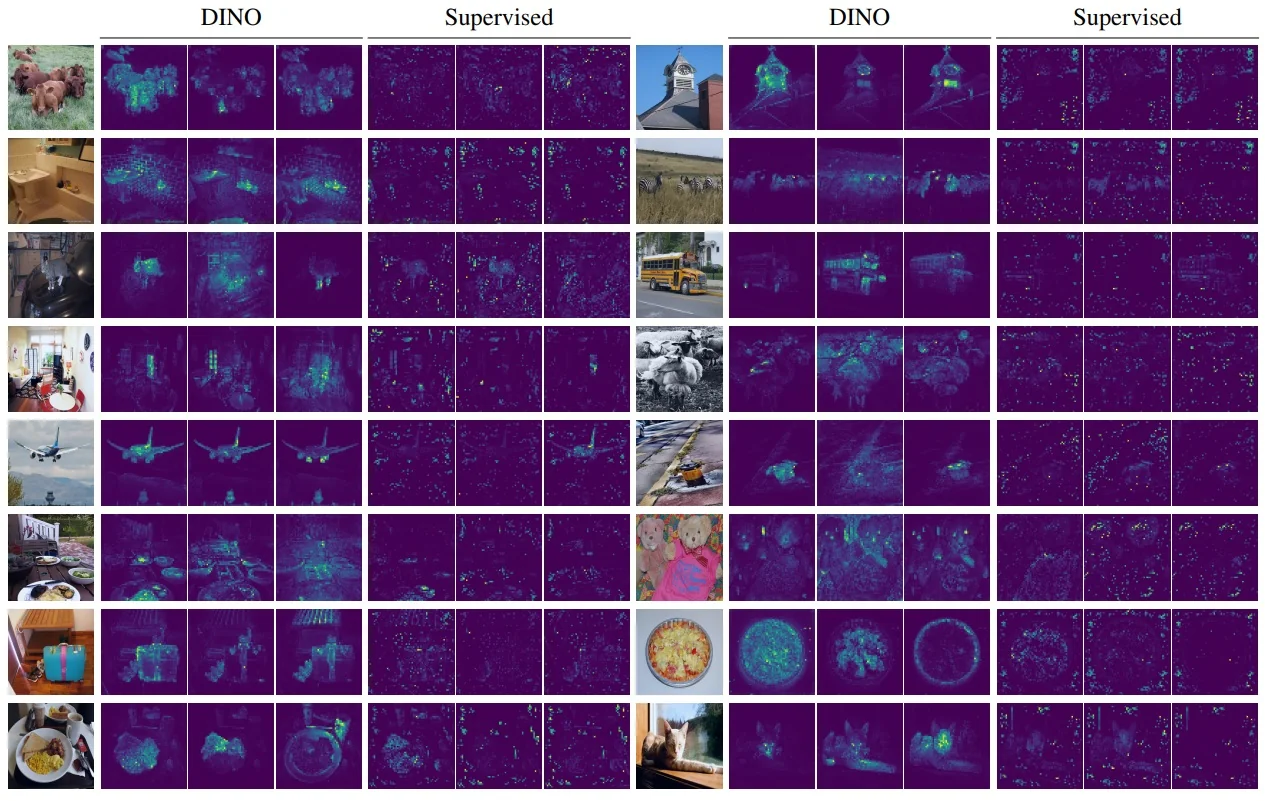
DINO’s attention behavior differs fundamentally. Its self-supervised objective aligns embeddings across augmentations rather than classes, implicitly encouraging the model to locate the entire object regardless of viewpoint. The result is an emergent ability to segment objects at a coarse level—without any annotation, supervision, or object priors. This qualitative ablation highlights the semantic richness of DINO’s representations compared to those learned under supervised training.
Ablation: Semantic Structure from Unlabeled Data A t-SNE projection of class-wise average features from DINO reveals clear semantic structure emerging from self-supervised training. The embeddings are computed by averaging [CLS] token outputs across all validation images in each ImageNet class. Even without labels, DINO organizes conceptually related categories into tight, coherent clusters.
In this subset of the full visualization, car-related categories such as minivan, sports car, and grille form a contiguous super-cluster—despite being distinct ImageNet classes. This is especially notable because a supervised model would be explicitly trained to pull these apart. DINO instead learns to preserve their visual proximity, discovering a shared abstraction of ”automobile” from raw pixels alone.
This behavior suggests that DINO builds representations that reflect the natural geometry of the visual world, rather than the boundaries imposed by classification labels. It captures both fine-grained distinctions and higher-order groupings, resulting in a structured embedding space where semantic similarity is preserved. This emergent clustering is a strong indicator of the model’s capacity for generalization and compositional reasoning.
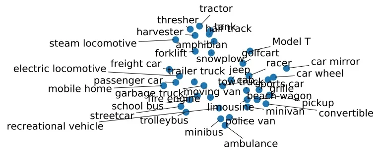
Ablation: Teacher Update Strategies DINO updates the teacher network via a momentum-based exponential moving average (EMA) of the student weights after each mini-batch. To evaluate this design choice, the authors compared several teacher variants: a frozen student copy, weights from the previous iteration, and weights from the previous epoch. Both the static and previous-iteration versions result in complete collapse, with top-1 k-NN accuracy near 0.1%. Interestingly, using the teacher from the previous epoch still achieves 66.6%, suggesting that smooth but temporally coherent updates suffice for learning. Nonetheless, the EMA momentum teacher yields the best results with 72.8% top-1 accuracy.
Throughout training, the EMA teacher consistently outperforms the student. Although both converge by the end, DINO evaluates downstream performance using the teacher encoder—a departure from prior approaches like BYOL and SimSiam that use the online student. This decision aligns with the observation that the teacher features are more stable and better structured during training.
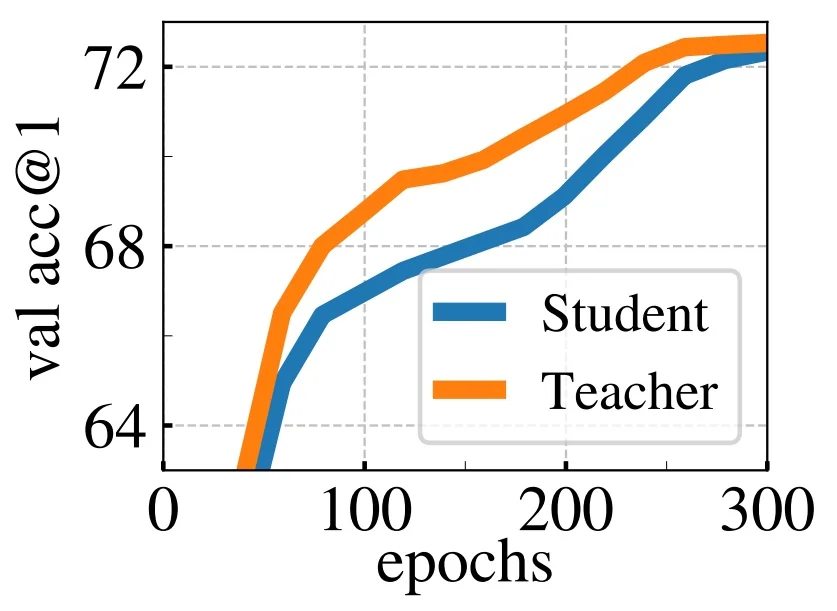
Ablation: Collapse Prevention via Centering and Sharpening To prevent representational collapse, DINO employs two distributional constraints on the teacher’s output: centering, which stabilizes the logit distribution, and sharpening, which encourages low-entropy predictions. As shown in the following figure, removing either component results in flat KL divergence between teacher and student, signaling collapse. Only when both are applied does the KL divergence rise—indicating informative learning. Centering alone or sharpening alone is insufficient. This explicit collapse prevention sets DINO apart from prior self-supervised methods that rely on architectural asymmetry or negative sampling.
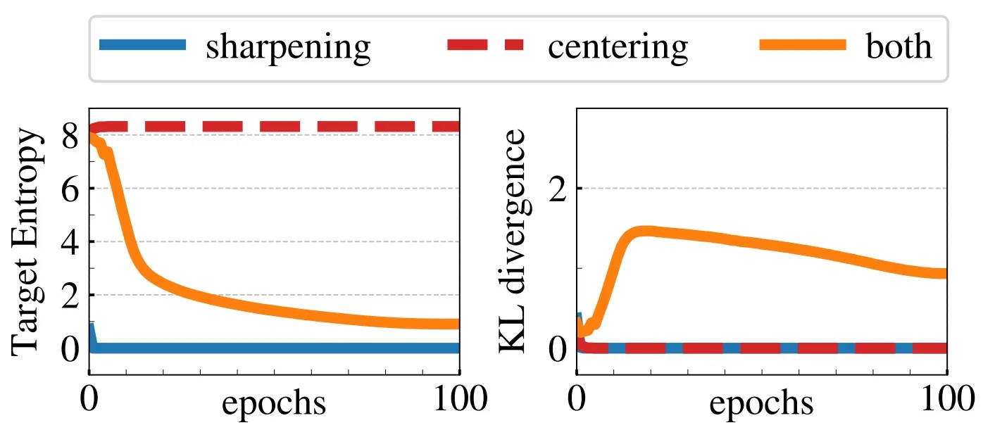
Ablation: Patch Size and Inference Throughput DINO’s Vision Transformer backbones allow tuning patch size to balance performance and efficiency. Smaller patches increase spatial resolution and token count, yielding higher accuracy but lower throughput. As seen in the following figure, ViT-B with \(8 \times 8\) patches significantly outperforms the \(16 \times 16\) baseline. However, reducing to \(5 \times 5\) yields negligible further gains while reducing throughput by over 4×. Thus, \(8 \times 8\) represents a strong tradeoff between accuracy and compute.
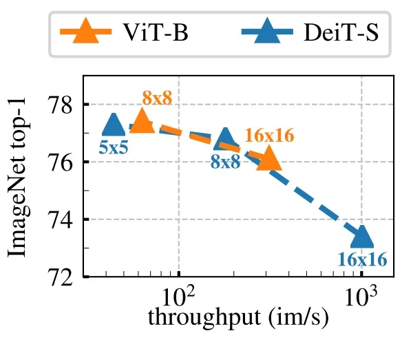
Ablation: Batch Size Effects Unlike contrastive methods such as SimCLR that require large batch sizes to generate diverse negatives, DINO adopts a BYOL-style architecture that enables stable training with significantly smaller batches. As shown in the below table, increasing the batch size from 128 to 1024 yields only a modest gain in top-1 k-NN accuracy—from 57.9% to 59.9%. This insensitivity to batch size makes DINO appealing for resource-constrained training setups, eliminating the need for large memory banks or massive batches.
| Batch Size | Top-1 k-NN Accuracy (%) |
|---|---|
| 128 | 57.9 |
| 256 | 59.1 |
| 512 | 59.6 |
| 1024 | 59.9 |
Ablation: Multi-Crop Augmentation and Resource Tradeoffs DINO relies heavily on the multi-crop augmentation strategy—combining two high-resolution global views with multiple low-resolution local views—to enforce scale-invariant learning. Increasing the number of local crops steadily improves accuracy but also increases compute and memory costs.
| Multi-Crop Configuration | Top-1 (100e) | Time (100e) | Top-1 (300e) | Time (300e) | Mem. (GB) |
|---|---|---|---|---|---|
| 2×224\(^2\) | 67.8% | 15.3h | 72.5% | 45.9h | 9.3 |
| 2×224\(^2\) + 2×96\(^2\) | 71.5% | 17.0h | 74.5% | 51.0h | 10.5 |
| 2×224\(^2\) + 6×96\(^2\) | 73.8% | 20.3h | 75.9% | 60.9h | 12.9 |
| 2×224\(^2\) + 10×96\(^2\) | 74.6% | 24.2h | 76.1% | 72.6h | 15.4 |
Paper Conclusion In summary, DINO achieves stable, predictor-free self-supervised learning through a carefully engineered interplay of functional asymmetries: centering, sharpening, a momentum-updated teacher, and a stop-gradient constraint. These mechanisms explicitly regulate entropy and variance in the teacher’s output, preventing collapse without requiring negative pairs or architectural tricks. Crucially, DINO’s design scales naturally to Vision Transformers and large-scale training, laying the foundation for more expressive, prototype-aware models. In the following part, we examine DINOv2, which extends this framework with dense patch-level supervision, stronger augmentations, and improved generalization across tasks and domains.
22.4.6 DINOv2: Learning Robust Visual Features Without Supervision
Background and Motivation DINOv2 [477] represents a decisive step forward in the development of general-purpose vision encoders trained without supervision. It builds on the architectural principles of DINO [70] while introducing two central innovations: first, a series of engineering improvements that enable stable training at scale—including techniques such as FlashAttention, sequence packing, and fully-sharded data parallelism (FSDP); and second, a novel data processing pipeline that yields a large, high-quality, balanced pretraining corpus.
The training strategy centers on a single, extremely large Vision Transformer (ViT-g/14, 1.1B parameters) pretrained on 142M carefully curated images (the LVD-142M dataset), whose representations are later distilled into smaller ViT models. Unlike CLIP-style models that rely on text-image supervision, DINOv2 is trained using only image data. This allows it to retain high-resolution, non-textual visual information that often goes unmentioned in captions. The authors argue—echoing a key insight from DINO—that purely visual supervision can uncover richer and more structured representations than those constrained by human-generated text.
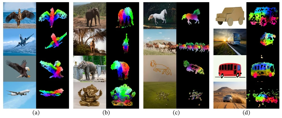
Emergent Semantic Structure Without Labels The visualization in Figure 22.44 reveals a remarkable capability: DINOv2’s patch-level representations exhibit emergent semantic correspondence across object categories and rendering styles. For example, bird wings and airplane wings are colored similarly, as are the heads of elephants and elephant-shaped statues. The model aligns photorealistic and sketched horses, or cartoon and real cars, segmenting analogous parts despite strong differences in appearance.
This behavior signals several breakthroughs. First, the model learns to perform unsupervised part segmentation without ever being given part annotations. Second, it displays invariance to pose, style, and texture—robustly recognizing object parts under transformations.
Third, the model appears to perform a form of cross-category analogical reasoning, matching functionally equivalent structures (e.g., “wheels” or “trunks”) across classes. Such analogical alignment is typically considered a hallmark of higher-level semantic understanding.
These emergent patterns strongly support the case for self-supervised pretraining at scale: DINOv2 shows that sufficiently powerful image-only models can learn both global and local features that are semantically structured, compositionally aware, and transferable across modalities, even without textual guidance.
Scaling Training through Architectural and Data Efficiency While DINOv2 inherits the foundational self-supervised architecture of its predecessor, its effectiveness stems in large part from practical advancements that make large-scale training both tractable and robust. The authors integrate optimizations such as FlashAttention, activation checkpointing, and fully sharded data parallelism (FSDP), enabling training with very large batch sizes—up to 2,048 samples per GPU on ViT-g/14. Large batches improve gradient estimation by reducing noise and encouraging optimization steps aligned with the full data distribution. This stabilizes training dynamics and improves convergence, especially in high-capacity models.
In contrast to earlier self-supervised models, which required either fine-tuning or domain adaptation to achieve high downstream performance, DINOv2 encoders are designed to be used off-the-shelf. Like other vision foundation models, they are pretrained on a large and diverse corpus of data and are intended to transfer broadly. In low-data regimes, the authors recommend freezing the backbone entirely and training only a lightweight task-specific head (e.g., a linear classifier or MLP). In medium-scale scenarios, selectively fine-tuning the final 1–3 transformer blocks is beneficial. Full fine-tuning is only advised when ample domain-specific data is available, as aggressive updates to a well-pretrained encoder may cause overfitting or degrade generalization.
Data Processing in DINOv2 To fully leverage the model’s architectural scale, DINOv2 introduces a sophisticated data processing pipeline that blends curated and uncurated image sources. As illustrated in the below figure, the process begins by embedding all images using a frozen ViT-H/14 model pretrained on ImageNet-22k. The uncurated images—often noisy or redundant—are first deduplicated using embedding similarity. Importantly, this step preserves semantic diversity while eliminating near-identical copies.
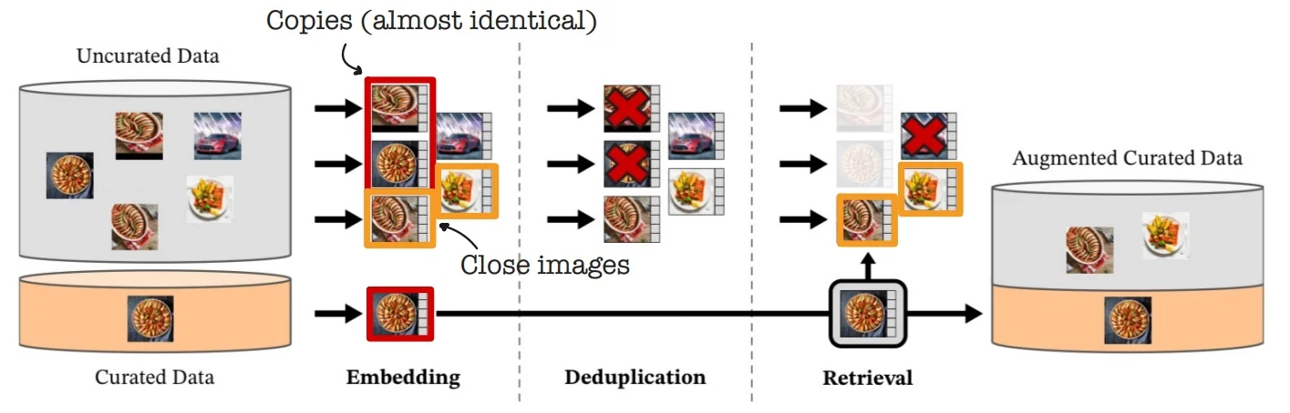
Next, a form of self-supervised retrieval is performed: curated datasets are used as anchors, and similar uncurated images are retrieved to augment them. This results in a large, semantically aligned dataset that preserves the controlled structure of curated corpora while scaling up with the diversity of web-scale data. The final product of this pipeline is the LVD-142M dataset, containing 142 million images from a wide range of visual domains, used to train the main DINOv2 encoders.
This deduplication and retrieval strategy relies on a strong self-supervised visual descriptor capable of identifying semantically near-duplicate images. To support this pipeline, the authors adopt a specialized copy detection model developed by FAIR: the Self-Supervised Copy Detection (SSCD) network [495]. Although the approximate nearest neighbor search uses the FAISS library for efficiency, the real innovation lies in the SSCD descriptor itself—an architecture that builds upon SimCLR with tailored modifications for identifying visual copies under heavy augmentation and corruption.
We now turn to the SSCD method, which serves as both a key enabler of DINOv2’s scalable data pipeline and an interesting contribution to self-supervised learning in its own right.
SSCD: A Self-Supervised Descriptor for Image Copy Detection
Motivation for Copy Detection in DINOv2 Robust copy detection is a foundational requirement in the DINOv2 data pipeline, which deduplicates over 600M web-crawled images to construct the 142M-image LVD-142M dataset [477]. Unlike standard image retrieval—where similarity scores yield a ranked list—copy detection requires confident binary decisions: is this image a transformed, compressed, or composited variant of a known one? False negatives allow redundant content to persist, reducing data efficiency; false positives are even more damaging, as they erroneously discard unique images and compromise dataset diversity. Thus, high recall and especially high precision are critical, with a preference for false negative tolerance over false positive risk.
To support this, DINOv2 adopts the Self-Supervised Copy Detection (SSCD) descriptors proposed by [495]. SSCD produces compact fixed-length embeddings that can be indexed for fast approximate nearest neighbor (ANN) search, and—crucially—are compatible with a single global cosine similarity threshold. This enables scalable deduplication across billions of comparisons without query-specific calibration or second-stage verification. Such invariance is essential in class-agnostic, internet-scale pipelines like DINOv2.
SSCD is built atop SimCLR but introduces two core modifications: (1) a mixed-positive contrastive loss, where all augmentations and synthetic composites (e.g., Mixup, CutMix) are treated as valid positives—enhancing robustness to occlusion and blending—and (2) a KoLeo entropy regularization term that maximizes differential entropy of the embedding distribution. The latter explicitly prevents representation collapse and spreads unrelated descriptors apart, tightening the cluster of true matches and creating a geometric “valley” in distance space where thresholding becomes reliable.
To evaluate SSCD, the authors report both mean Average Precision (mAP) and micro Average Precision (µAP). mAP measures the per-query ranking quality of retrieval. For each query image \( q \), the system returns a ranked list of \( N_q \) candidate matches from the dataset, sorted in decreasing similarity (i.e., most likely copies first). The rank \( k \) of a result denotes its position in this list: the topmost candidate has rank 1, the second has rank 2, and so on.
The value of \( N_q \) is a configurable hyperparameter: it reflects how many candidates are retrieved and scored per query. In practice, \( N_q \) is typically fixed across all queries and chosen to be large enough to include all true positives (if possible) while limiting computational cost.
For example, SSCD experiments on DISC2021 retrieve the top \( N_q = 1000 \) candidates for each query using approximate nearest neighbor (ANN) search. If a true match does not appear within the top \( N_q \), it is treated as a false negative for AP computation. Thus, larger \( N_q \) values increase the chance of recovering more true positives but can also dilute early precision and raise evaluation cost.
Given the candidate list of length \( N_q \), the average precision (AP) for query \( q \) is defined as: \[ \mbox{AP}(q) = \frac {1}{|\mathcal {P}_q|} \sum _{k \in \mathcal {P}_q} \frac {\mbox{TP}(k)}{k}, \] where:
- \( \mathcal {P}_q \subseteq \{1, 2, \ldots , N_q\} \) is the set of ranks where true positives (matching images) appear,
- \( \mbox{TP}(k) \) is the number of true positives found in the top \( k \) positions.
This formula averages the precision at each rank where a correct match is retrieved, rewarding systems that place true copies earlier in the list. The final mAP is computed by averaging over all queries: \[ \mbox{mAP} = \frac {1}{Q} \sum _{q=1}^{Q} \mbox{AP}(q), \] where \( Q \) is the total number of query images. This is analogous to the mAP used in object detection benchmarks such as COCO or Pascal VOC, except that here the queries are images rather than object classes, and relevant items are copy instances rather than bounding boxes.
While increasing \( N_q \) can marginally improve recall, it does not affect the shape of the precision–recall curve beyond the first few true matches. In copy detection, the ability to retrieve true copies near the top of the ranked list—rather than deep in the tail—is what determines retrieval quality. Hence, SSCD is evaluated with fixed \( N_q \) (e.g., 1000) across all queries to ensure fair comparison and practical relevance.
In contrast to mAP, which computes a per-query precision–recall curve before averaging, micro Average Precision (µAP) aggregates predictions globally across all queries and candidates. Rather than evaluating how well the system ranks results for each query independently, µAP assesses the overall binary classification performance under a single decision rule: declare a match if the similarity score \( s \geq \tau \), and a non-match otherwise.
In practical terms, µAP is computed as follows:
- 1.
- Compute similarity scores (e.g., cosine similarity) and ground truth labels for all query–candidate pairs.
- 2.
- Pool all scored pairs into a single list, ignoring which query each pair originated from.
- 3.
- Sort this list in descending order of similarity score.
- 4.
- Sweep over the list from highest to lowest score, tracking cumulative true positives (TP), false positives (FP), and false negatives (FN).
- 5.
- At each step, compute global precision and recall: \[ \mbox{Precision}_{\mbox{micro}} = \frac {\mbox{TP}}{\mbox{TP} + \mbox{FP}}, \quad \mbox{Recall}_{\mbox{micro}} = \frac {\mbox{TP}}{\mbox{TP} + \mbox{FN}}. \]
- 6.
- Plot the global precision–recall curve and compute the area under this curve: \[ \mbox{µAP} = \int _0^1 \mbox{Precision}_{\mbox{micro}}(\mbox{Recall}_{\mbox{micro}}) \, d\mbox{Recall}_{\mbox{micro}}. \]
This process treats every prediction equally, regardless of which query it is associated with. For large-scale systems such as DINOv2, which apply a fixed cosine similarity threshold \( \tau \) across billions of comparisons during deduplication, µAP provides a more faithful estimate of system-level performance than mAP. It directly answers: How well does a single global threshold perform across the entire dataset?
Why SSCD is optimized for µAP. The Self-Supervised Copy Detection (SSCD) framework is explicitly trained to maximize separability under a global threshold. Its loss function includes:
- An InfoNCE contrastive loss, which pulls together positive pairs (transformed versions of the same image) and pushes apart negatives.
- A KoLeo entropy regularization term, which spreads descriptors uniformly across the embedding space, encouraging a high-entropy representation and avoiding collapse.
Together, these losses reshape the representation space so that:
- True copies form tight, isolated clusters with high similarity scores (near 1),
- Distractors are pushed to lower similarity regions,
- The resulting histogram of cosine similarities becomes bimodal, with a pronounced “decision valley” between the two modes.
This structure enables the use of a single, global decision threshold \( \tau \) that robustly separates matches from non-matches. µAP, by design, is sensitive to exactly this kind of calibration. In the case of DINOv2, high µAP scores indicate that SSCD’s learned descriptors remain discriminative even when evaluated at scale, under a uniform threshold shared across the dataset.
In practice, DINOv2 retrieves nearest neighbors using fast ANN search and applies a fixed cosine similarity cutoff to identify duplicates. There is no per-query re-ranking, no heuristic tuning, and no label supervision—just a binary decision. µAP therefore serves not merely as an evaluation score, but as a direct proxy for end-to-end deduplication success.
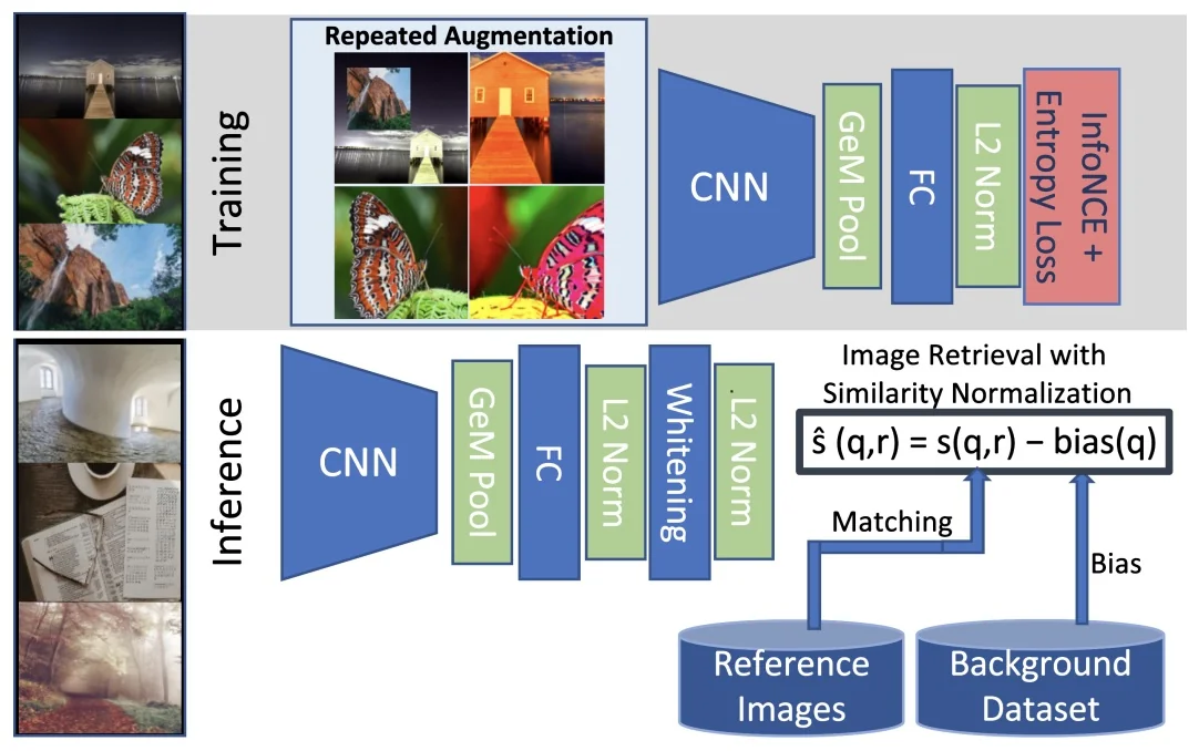
SSCD enables this system to scale while preserving data quality, producing clean, non-redundant datasets like LVD-142M that fuel generalization across downstream tasks.
Core Architecture and Augmentations The Self-Supervised Copy Detection (SSCD) framework adapts the SimCLR dual-branch design into a pipeline tailored for large-scale instance-level copy detection. From a single image, two heavily augmented views are generated using aggressive transformations. Each view is then passed through a shared convolutional encoder—typically a ResNet-50 or ResNeXt-101—which maps the input into a dense feature map \( \mathbf {F} \in \mathbb {R}^{C \times H \times W} \).
To transform the spatial feature map into a compact, fixed-length descriptor, SSCD uses Generalized Mean (GeM) pooling—a flexible alternative to average or max pooling. GeM introduces a learnable exponent \( p \) that determines how much weight is given to high-activation regions within each channel of the feature map: \[ \mbox{GeM}(\mathbf {F})_c = \left ( \frac {1}{HW} \sum _{h=1}^H \sum _{w=1}^W (F_{c,h,w})^p \right )^{\frac {1}{p}} \] This expression reduces to average pooling when \( p = 1 \) and increasingly resembles max pooling as \( p \to \infty \). By learning \( p \) directly from data, the network adapts its pooling behavior: lower \( p \) values yield globally averaged features that are robust to noise and distributed edits, while higher \( p \) values concentrate attention on localized peaks—useful for detecting inserted objects, watermarks, or tampering artifacts.
This ability to interpolate between diffuse and selective aggregation is particularly valuable in copy detection, where relevant cues may range from small, high-frequency details to global scene-level structures. In practice, SSCD uses a single shared \( p \) across all channels (typically initialized at \( p = 3 \)), striking a stable balance between sensitivity and robustness across diverse manipulation types.
The pooled vector is passed through a lightweight projection head (typically a two-layer MLP) that outputs a compact descriptor of fixed dimension (e.g., 128 or 512). Unlike SimCLR, which discards this projection head during inference, SSCD retains it since the output descriptor is used directly for retrieval. This vector is then \(\ell _2\)-normalized: \[ \mathbf {z} \leftarrow \frac {\mathbf {z}}{\|\mathbf {z}\|_2} \] This normalization ensures metric compatibility and stabilizes the contrastive objective. Together, the encoder, GeM pooling, and retained projection head form a compact and robust representation pipeline—yielding descriptors resilient to occlusion, compression, content insertion, and other real-world manipulations.
Post-Processing via Whitening and Synergy with Training The final stage in SSCD’s inference pipeline is a whitening transformation, applied after L2 normalization to all output descriptors. Whitening reshapes the learned embedding space to be statistically isotropic, removing both mean and correlation bias across dimensions. Each descriptor \( \mathbf {z} \in \mathbb {R}^d \) is transformed using precomputed dataset-wide statistics—namely, the empirical mean \( \boldsymbol {\mu } \) and covariance matrix \( \boldsymbol {\Sigma } \), computed once over a large corpus of descriptors—via: \[ \mathbf {z}_{\mbox{whitened}} = \boldsymbol {\Sigma }^{-1/2} (\mathbf {z} - \boldsymbol {\mu }) \]
This transformation serves three core functions. First, it standardizes the descriptor space by decorrelating feature dimensions and equalizing their variance, so that all directions contribute equally to similarity computations. Second, it enforces isotropy—an assumption underpinning the efficiency of large-scale retrieval systems such as IVF-PQ and HNSW. Third, it mitigates dimensionality collapse, a common issue in contrastive models where variance concentrates along only a few axes, reducing the expressiveness of the embedding space.
One might ask why whitening is applied only at inference. The answer lies in the scale and stability of the required statistics: computing \( \boldsymbol {\mu } \) and \( \boldsymbol {\Sigma } \) over entire datasets yields reliable global structure, whereas attempting whitening over per-batch covariance during training would be noisy, unstable, and poorly aligned across steps. Moreover, whitening is a linear and invertible transformation; it preserves the semantic topology learned during training—merely reorienting it into a more favorable coordinate system.
Importantly, SSCD is not reliant on whitening to fix its representations post hoc. During training, it integrates differential entropy regularization, which encourages descriptors to spread uniformly over the hypersphere. This regularizer acts as a counterforce to the contrastive loss: while InfoNCE pulls positives together and pushes negatives apart, entropy regularization ensures that the overall space remains high-rank, well-distributed, and robust against collapse. Crucially, this does not destroy the discriminative structure. The entropy term’s influence is strongest locally—discouraging clustering of unrelated samples—while allowing global structure (e.g., semantic clusters) to form freely.
The result is a learned representation that is already near-isotropic before whitening is applied. The post-training whitening step thus introduces minimal distortion: it subtly aligns the learned geometry with the assumptions of downstream search algorithms, improving recall and stability without degrading feature quality. Eigenvalue clipping ensures numerical robustness, and whitening is performed at the full descriptor size—without PCA compression—thanks to the high effective dimensionality induced by the entropy-aware training.
Together with SSCD’s other architectural elements—aggressive augmentations, GeM pooling for adaptive saliency control, and a retained projection head for stable inference—whitening forms the final normalization layer that makes descriptors compact, expressive, and ready for high-throughput image retrieval.
We now turn to the augmentation pipeline that enables SSCD to simulate real-world tampering scenarios, further enhancing its robustness to both local edits and composite manipulations.
Augmentation Pipeline for Real-World Tampering To simulate the types of transformations encountered in real-world copy detection (e.g., memes, image edits, composites), SSCD uses an aggressive and diverse set of data augmentations. These include common distortions such as JPEG compression, Gaussian blur, perspective shifts, text overlays, and emoji insertions. More uniquely, SSCD incorporates mixed-image augmentations—specifically, CutMix and Mixup—which blend content from two or more images into one. This simulates adversarial cases such as content repurposing or collage creation.
These augmentations play a dual role. First, they force the model to focus on truly discriminative visual content, rather than spurious correlations like background texture. Second, they expand the definition of “positive pairs” during contrastive training: for example, an image and its Mixup blend are treated as semantically related, reinforcing robustness to visual mixing.
The inclusion of such augmentations is not just a heuristic—it is a principled way to operationalize invariance to partial copying and compositional edits, which are frequent in copy detection use cases.
Loss Formulation with Entropy and Mixed Positives SSCD departs from standard SimCLR in two complementary and carefully designed ways. First, it extends the InfoNCE contrastive loss to support composite positives—image views blended via CutMix or MixUp that contain content from multiple source images. Second, it introduces a differential entropy regularization term to prevent representation collapse and encourage a well-spread, high-entropy embedding space suitable for threshold-based copy detection.
In the modified contrastive loss, any descriptor \( z_i \) derived from a mixed view treats all of its donor images as positives. This is formalized by defining \( \mathcal {P}_i \) as the set of all positive indices for anchor \( z_i \), yielding the following loss:
\[ \mathcal {L}_{\mbox{InfoNCE}_{\mbox{mix}}} = - \frac {1}{2N} \sum _{i=1}^{2N} \frac {1}{|\mathcal {P}_i|} \sum _{j \in \mathcal {P}_i} \log \frac {\exp (\mbox{sim}(z_i, z_j)/\tau )}{\sum _{k \notin \hat {P}_i} \exp (\mbox{sim}(z_i, z_k)/\tau )} \]
Here, \( \hat {P}_i \) includes both traditional augmentations and all donor views contributing to a mixed image. This encourages the model to learn semantic consistency across partial overlaps and cut-and-paste transformations—crucial for robustness in copy detection scenarios.
To complement this broadened notion of positive alignment, SSCD introduces an entropy-based regularizer that governs the global geometry of the embedding space. Without this, contrastive objectives can induce dimensionality collapse, where descriptors concentrate in a narrow subspace, reducing expressiveness and degrading thresholdability.
SSCD addresses this by incorporating a differential entropy regularizer based on the Kozachenko Leonenko (KoLeo) estimator. While the entropy of a continuous distribution \( p(x) \) is defined as: \[ H(p) = - \int p(x) \log p(x) \, dx, \] this integral is intractable in high dimensions. The KoLeo estimator instead penalizes geometric crowding, using nearest-neighbor distances among non-positives to encourage spread. The entropy loss is given by: \[ \mathcal {L}_{\mbox{KoLeo}} = \frac {1}{N} \sum _{i=1}^{N} \log \min _{j \notin \hat {P}_i} \| z_i - z_j \|_2, \] where nearest neighbors are restricted to negatives to preserve alignment. This term incentivizes descriptors to be well-separated globally, mitigating collapse and encouraging full use of the unit hypersphere.
The entropy regularization thus plays a dual geometric role: it prevents collapse by distributing descriptors uniformly and enhances discriminability by separating unrelated images. These properties are especially valuable for copy detection, where small transformations or content reuse must be detected without confounding semantically unrelated instances. By pulling positives together while pushing negatives apart, SSCD constructs an embedding space that is both locally tight—for precise alignment—and globally uniform—to support robust thresholding.
The final SSCD objective integrates both components: \[ \mathcal {L}_{\mbox{SSCD}} = \mathcal {L}_{\mbox{InfoNCE}_{\mbox{mix}}} + \lambda \cdot \mathcal {L}_{\mbox{KoLeo}}, \quad \mbox{with (default) } \lambda = 30 \]
This constructive tension yields a descriptor space well-calibrated for large-scale, threshold-based copy detection: true variants of an image form tight clusters, while distractors—even if visually similar—are geometrically repelled. This embedding structure is critical for scalable applications like DINOv2, where deduplication must operate efficiently over hundreds of millions of images using a single global threshold without task-specific tuning.
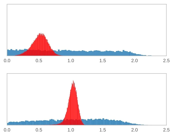
Empirical Results and Impact SSCD delivers strong empirical gains across multiple copy detection benchmarks. On DISC2021, it improves over SimCLR by more than +48% in micro Average Precision (µAP), reflecting dramatically better thresholded separation between copies and distractors. On the Copydays dataset, SSCD achieves 86.6 mAP using a ResNet-50 backbone, and up to 93.6 mAP with a ResNeXt—substantially outperforming prior contrastive and retrieval-based approaches, including Multigrain and DINO. These results establish SSCD as a state-of-the-art self-supervised descriptor for real-world copy detection tasks.
In addition to accuracy, SSCD is designed with deployment in mind. It produces lightweight descriptors (e.g., 512 dimensions), incorporates internal score normalization for calibration, and supports TorchScript export for efficient inference.
This combination of effectiveness and scalability is precisely what makes SSCD suitable for DINOv2’s deduplication pipeline: applying a single, global cosine threshold to SSCD descriptors filters redundant content across hundreds of millions of web images. The result is LVD-142M—a large-scale, clean, and highly diverse dataset that forms the foundation of DINOv2’s training corpus.
Yet while deduplication solves the problem of data redundancy, it leaves open the deeper challenge of data understanding. SSCD focuses on instance-level discrimination via global descriptors, sufficient for matching near-duplicates—but inadequate for learning rich, hierarchical representations that capture objects, parts, textures, and spatial relations. To train a general-purpose vision model, DINOv2 must extract meaning not only from entire images, but also from their internal structure.
This is the motivation for DINOv2’s second key design pillar: Masked Image Modeling (MIM). Inspired by masked language modeling in NLP—where models learn to predict missing words from surrounding text—MIM applies a similar principle to images: it randomly masks a subset of input patches and trains the model to infer the missing content based on the visible context. This compels the model to develop a structured understanding of spatial relationships, textures, object parts, and semantic composition. Rather than simply recognizing whole-image identities, the model must learn to reconstruct or predict image regions in a way that reflects the underlying scene structure. As a result, MIM encourages the emergence of rich, localized, and hierarchically organized representations—properties essential for dense prediction, compositional reasoning, and generalization across domains.
In the remainder of this part, we examine how DINOv2 incorporates MIM into its self-supervised learning framework. We begin by revisiting the Masked Autoencoders (MAE) [219] approach, which demonstrates that scalable and transferable visual representations can be learned by reconstructing raw pixels over randomly masked patches using a simple asymmetric encoder–decoder architecture. MAE’s high masking ratio and efficient training design make it a compelling base for large-scale vision pretraining. We then turn to iBOT [819], which extends the MIM paradigm by combining masked patch prediction with self-distillation. Instead of predicting pixels, iBOT trains a student network to match the patch-level and class-level outputs of a momentum teacher network, using a contrastive formulation that unifies local and global supervision. This dual-objective structure not only improves semantic alignment across views but also enhances token-level understanding—an architectural strategy that DINOv2 ultimately adopts and refines.
As we will see, the full DINOv2 objective integrates iBOT-style masked token prediction with global self-distillation and entropy-based regularization, resulting in a unified framework that learns strong, scalable, and semantically rich visual representations without labels.
Masked Autoencoders (MAE): Scalable Vision Learners
Masked Autoencoders (MAE) [219] introduced a scalable and generative alternative to contrastive self-supervised learning, drawing inspiration from masked language modeling in NLP. At the time, leading methods such as MoCo and SimCLR trained models to discriminate between augmented views of different images—a strategy that produced linearly separable features suitable for linear probing, where a simple linear classifier is trained on top of a frozen backbone for downstream tasks like ImageNet classification. In contrast, MAE proposed to reconstruct missing parts of an image, training a Vision Transformer (ViT) to generate masked regions from a sparse set of visible patches. This approach shifted the focus from view discrimination to generative modeling, emphasizing content recovery and holistic understanding.
Two key innovations underpinned MAE’s success. First, the model uses a high masking ratio—typically 75%—which makes the reconstruction task challenging and encourages the encoder to capture global semantic structure. Second, it employs an asymmetric encoder–decoder architecture: the encoder processes only visible patches, while a lightweight decoder reconstructs the full image using both the encoded tokens and learnable mask tokens. This design reduces computation significantly—for example, a ViT processing 196 image patches will encode only 49, lowering the cost of quadratic attention. The decoder is discarded after pre-training.
MAE achieves state-of-the-art performance when the pretrained model is fully fine-tuned, meaning all weights are updated for the target task. For instance, ViT-L and ViT-H models pretrained with MAE reach 85.9% and 87.8% top-1 accuracy on ImageNet-1K, respectively. However, MAE performs poorly under linear probing: its features are not well organized for simple linear separation. This reveals a trade-off—MAE learns rich, dense representations that support fine-tuning, but they are less directly usable in frozen, plug-and-play settings.
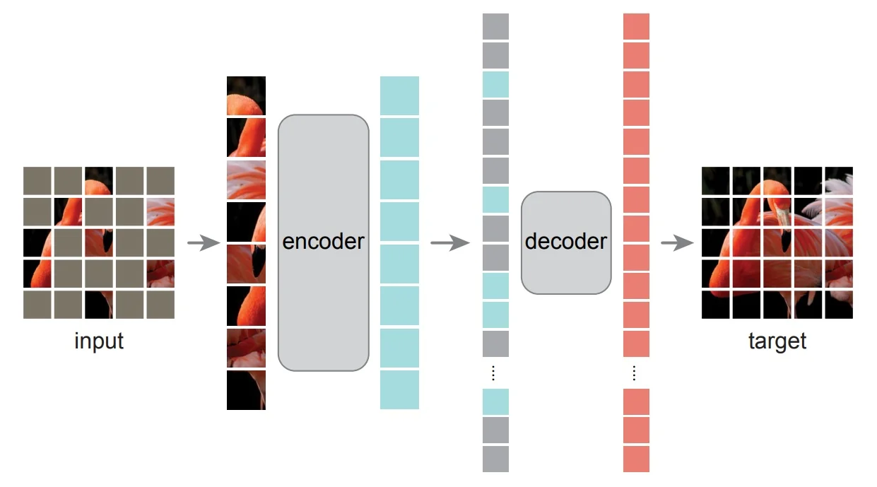
This trade-off invites a deeper look into MAE’s core architecture and training dynamics. In the parts that follow, we examine the asymmetric encoder–decoder design, the pixel-level reconstruction loss, empirical findings from ablation studies, and qualitative insights from image reconstructions. These components not only reveal how MAE enables efficient, scalable pre-training but also explain its limitations in producing linearly separable features. These very limitations would later motivate hybrid approaches—such as iBOT and DINOv2—that build upon MAE’s generative backbone while introducing discriminative signals to enhance semantic structure in the learned representations.
Asymmetric Architecture and High-Ratio Masking The MAE framework is built upon two foundational principles: a high masking ratio that removes most of the input image, and an asymmetric encoder–decoder architecture that enables efficient training and scalable inference. Together, these choices define a powerful generative pretext task for self-supervised learning.
Given an input image of size \(224 \times 224\), MAE first partitions it into non-overlapping patches of size \(16 \times 16\), yielding \(N = 196\) total patches. A random subset comprising \(rN\) patches is masked, typically with a high masking ratio \(r = 0.75\), leaving \(V = (1 - r)N = 49\) visible patches. This high ratio ensures that reconstructing the missing content requires more than low-level interpolation; it compels the model to infer semantic structure from sparse observations.
Encoder. The encoder is a standard Vision Transformer (ViT), modified to operate solely on the visible subset of patches. Each visible patch is linearly projected into a \(d\)-dimensional token (e.g., \(d = 768\) for ViT-Base) and combined with its positional embedding, yielding a sequence \(\mathbf {x}_v \in \mathbb {R}^{V \times d}\). This sequence is processed by the encoder \(f_\theta \) to produce latent representations: \[ \mathbf {z}_v = f_\theta (\mathbf {x}_v) \in \mathbb {R}^{V \times d}. \] This architectural asymmetry is critical: by removing masked tokens from the encoder input, MAE reduces the self-attention cost from \(\mathcal {O}(N^2)\) to \(\mathcal {O}(V^2)\). Since \(V\) is just a quarter of \(N\), this translates to an approximate \(16\times \) reduction in attention overhead. Such savings enable efficient pre-training of large models like ViT-L and ViT-H without relying on specialized sparse operations. Additionally, by excluding mask placeholders, the encoder is encouraged to build robust semantic representations from incomplete and irregular visual input—promoting holistic understanding instead of overfitting to token identity. Meanwhile, a lightweight decoder—typically just 1–8 Transformer blocks with reduced width (e.g., 512)—is used to reconstruct the masked content without overwhelming the overall computational cost.
Decoder. The decoder in MAE is a lightweight Transformer that operates only during the pre-training phase. Its purpose is to reconstruct the full set of \(N\) image patches—including the masked ones—based on the sparse, high-level features extracted by the encoder. The decoder receives as input:
- the encoded visible tokens \(\mathbf {z}_v \in \mathbb {R}^{V \times d}\),
- \(rN\) copies of a shared, learned mask token \(\mathbf {m} \in \mathbb {R}^{1 \times d}\), and
- positional embeddings \(\mathbf {p} \in \mathbb {R}^{N \times d}\) associated with the original patch positions.
The key design choice is that all masked positions share the same learnable vector \(\mathbf {m}\)—that is, there is no position-specific or image-dependent masking embedding. This simplification ensures that the decoder must rely on the context provided by the visible tokens and their positional relationships to generate plausible reconstructions.
To reassemble the full patch sequence, the \(V\) visible tokens and \(rN\) mask tokens are merged and sorted according to their original spatial indices. After positional embeddings are added, the resulting sequence of shape \(\mathbb {R}^{N \times d}\) is passed through a shallow Transformer decoder \(g_\phi \): \[ \hat {\mathbf {x}} = g_\phi \left ( \mbox{sort}\left ( [\mathbf {z}_v; \mathbf {m}^{(rN)}] + \mathbf {p} \right ) \right ), \] where \(\mathbf {m}^{(rN)}\) denotes the broadcasted mask token repeated \(rN\) times, and \(\hat {\mathbf {x}} \in \mathbb {R}^{N \times d}\) is the output feature map representing all patches, reconstructed into patch embedding space.
The decoder is intentionally shallow and narrow—typically just 4–8 Transformer blocks with lower embedding dimension (e.g., 512)—because its role is to convert semantic context into low-level pixel estimates, not to learn general-purpose representations.
Loss. The reconstruction target is the original (normalized) pixel content of each masked patch. Let \(\tilde {\mathbf {x}}_i \in \mathbb {R}^d\) denote the ground-truth target for masked patch \(i\), and let \(\hat {\mathbf {x}}_i\) be the decoder’s prediction. The loss is a mean squared error (MSE) computed only over the masked patches: \[ \mathcal {L}_{\mbox{MAE}} = \frac {1}{rN} \sum _{i \in \mathcal {M}} \left \| \hat {\mathbf {x}}_i - \tilde {\mathbf {x}}_i \right \|_2^2, \] where \(\mathcal {M}\) is the set of indices corresponding to masked patches. By excluding visible patches from the loss, the model is forced to rely on contextual reasoning rather than simply memorizing input-output pairs. Despite using a low-level reconstruction target (pixels), this strategy leads to strong high-level features in the encoder, especially when followed by supervised fine-tuning.
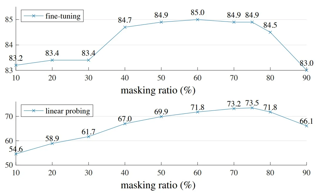
After pre-training, the decoder is discarded entirely. For downstream recognition tasks, the encoder is reused in isolation and applied to the unmasked, full image. Its output—obtained either from a class token or global average pooling—serves as the learned representation for tasks such as classification, detection, or segmentation. This asymmetry ensures that representational power is concentrated in the encoder, promoting strong transferability while minimizing deployment overhead.
In summary, MAE’s encoder–decoder structure is deliberately optimized for both scalability and semantic richness. The encoder learns to infer high-level representations from sparse, context-limited views of the image, while the decoder performs a minimalistic reconstruction task.
Empirical Results and Qualitative Analysis The MAE paper provides both qualitative and quantitative evidence for the effectiveness of masked autoencoding as a pretext task. A central finding is that MAE learns holistic and semantically meaningful representations, even when only a small subset of input patches is visible.
Qualitative Reconstructions: MAE’s reconstructions from highly masked images are not pixel-perfect but are often semantically plausible. As illustrated in Figure 22.50, the model can infer the coarse structure, object category, and spatial layout of missing regions, despite having access to only 20–25% of the original patches.
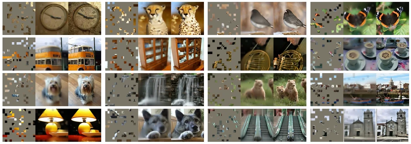
The reconstructions tend to be blurry, a known consequence of using an MSE loss in pixel space, which averages over plausible outcomes. Nonetheless, these results confirm that the encoder has learned high-level features of object geometry and context.
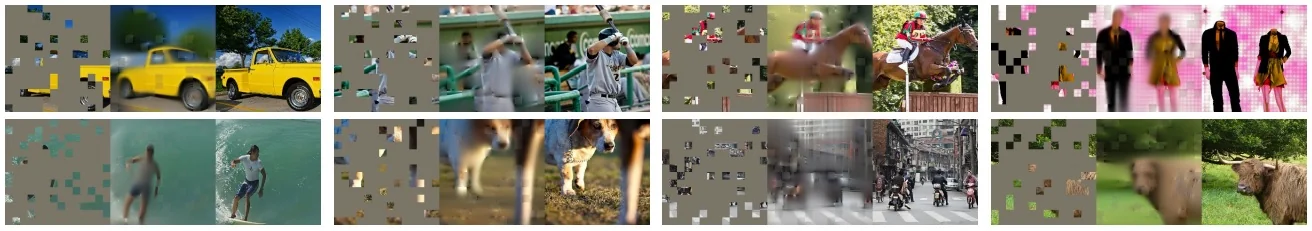
Robustness to Higher Masking Ratios: Even when masking exceeds 85–95%, the model is still able to reconstruct scenes with recognizable structure, as shown in Figure 22.52. This demonstrates that the encoder has internalized robust priors over image composition and semantics, which emerge naturally from the self-supervised objective.
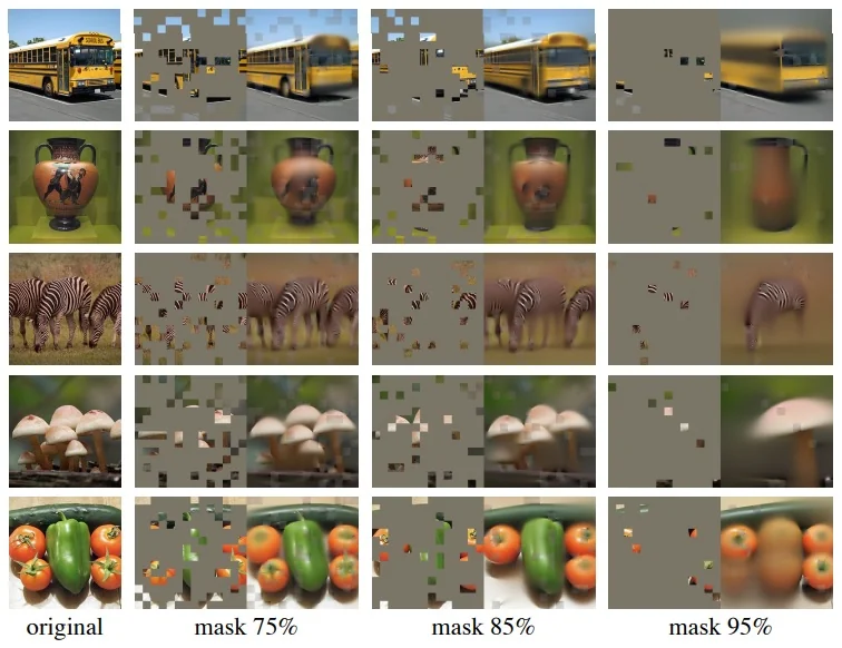
Importantly, the choice of random masking is not incidental. Structured masking schemes such as grid-wise or block-wise remove spatial redundancy less effectively, enabling shortcut learning and degrading the semantic quality of representations. Randomly sampling patches without replacement eliminates these correlations and compels the model to develop better representations.
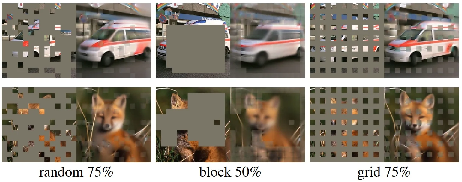
Masked Autoencoders (MAEs) have established themselves as a scalable and efficient framework for self-supervised learning. Their asymmetric encoder–decoder design and high masking ratio (typically 75%) enable lightweight training even with large ViT backbones such as ViT-L and ViT-H. However, while MAEs excel in downstream fine-tuning tasks, they exhibit a fundamental limitation in frozen representation quality.
This becomes evident in linear probing evaluations. A ViT-L model trained with MAE achieves only \(75.8\%\) top-1 accuracy on ImageNet, whereas contrastive and distillation-based methods fare significantly better: MoCo v3 reaches \(77.6\%\) with ViT-L, and DINO achieves \(80.1\%\) with the smaller ViT-B/8. This discrepancy reflects a core issue with MAE’s pixel-level reconstruction loss: although it drives the learning of rich, transferable features, these features are not organized in a semantically aligned or linearly separable manner. The encoder is optimized for reconstruction fidelity, not classification utility.
Ablation Studies: The following ablations from [219] offer empirical insight into this behavior, highlighting which architectural decisions contribute to performance gains—and where limitations persist:
- Decoder depth and width: Increasing decoder depth substantially improves linear probing (\(+8.0\%\)) but barely affects fine-tuning. This suggests the pixel-level target lacks semantic pressure for linear alignment.
- Mask token placement: Including masked tokens in the encoder severely harms both accuracy and efficiency.
- Reconstruction target: Normalized pixels outperform both raw pixels and discrete token targets (e.g., dVAE from BEiT).
- Data augmentation: MAE performs well even with minimal augmentation, unlike contrastive methods which depend heavily on strong augmentation pipelines.
- Masking strategy: Random sampling significantly outperforms structured block or grid masking.
| Component | Setting | Fine-tuning (%) | Linear Probing (%) |
|---|---|---|---|
| Decoder Depth | 8 blocks vs. 1 block | \(+0.1\) | \(+8.0\) |
| Decoder Width | 512-d vs. 256-d | \(-0.1\) | \(-1.6\) |
| Mask Token (Encoder) | w/ token vs. w/o | \(-0.4\) | \(-14.1\) |
| Target Type | Norm. pixels vs. unnorm. | \(+0.5\) | \(+0.4\) |
| Data Augmentation | Crop vs. Crop + jitter | \(-0.4\) | \(-2.4\) |
| Masking Strategy | Random vs. Block | \(-2.1\) | \(-10.9\) |
| Masking Ratio | 75% vs. 50% | \(-0.5\) | \(-17.5\) |
These findings reinforce MAE’s strengths in architectural simplicity and scalability, but also underscore the need for learning objectives that promote semantic alignment. The gap in linear separability—despite strong reconstruction and transfer performance—motivates the development of hybrid approaches that retain MAE’s architectural benefits while improving the discriminative structure of the learned features.
To address this, iBOT [819] introduces a unifying framework that combines MAE’s masking-based efficiency with the self-distillation paradigm of DINO. Instead of predicting pixels, iBOT casts masked image modeling as a semantic feature prediction task. A student network is trained to match the outputs of a momentum-updated teacher network on two levels:
- Patch-level distillation: For masked regions, the student predicts the teacher’s soft feature distributions using cross-entropy, improving local semantic alignment.
- Global self-distillation: The student’s [CLS] token is trained to match the teacher’s [CLS] token across multiple augmented views, using the DINO objective.
This approach effectively replaces MAE’s low-level regression loss with high-level classification objectives, enabling the model to learn both localized visual concepts and globally coherent features. The result is significantly improved linear separability and enhanced performance in frozen transfer settings.
Within the broader self-supervised landscape, iBOT serves as the architectural and algorithmic bridge to DINOv2. DINOv2 inherits iBOT’s dual-objective design—combining masked feature prediction with global alignment—and extends it with entropy-based regularization techniques such as centering and KoLeo. This synthesis enables stable and scalable pretraining, producing general-purpose visual representations that match or exceed supervised baselines in both fine-tuned and frozen evaluations.
iBOT: Masked Image Modeling with Self-Distillation
iBOT [819] advances masked image modeling by combining the token-masking strategy introduced in MAE with the self-distillation framework of DINO. While MAE relies on an asymmetric encoder–decoder design to reconstruct masked image patches at the pixel level, iBOT reformulates the task as semantic feature prediction. Architecturally, it adopts a symmetric, Siamese-style setup with two Vision Transformers—a student and a momentum-updated teacher—mirroring DINO’s design. The student receives a masked image and is trained to match the teacher’s soft output distributions at both the patch level (for masked tokens) and the image level (via the [CLS] token). This dual-objective formulation preserves MAE’s efficiency in masking-based supervision while promoting the discriminative alignment necessary for strong frozen transfer performance—without requiring task-specific fine-tuning.
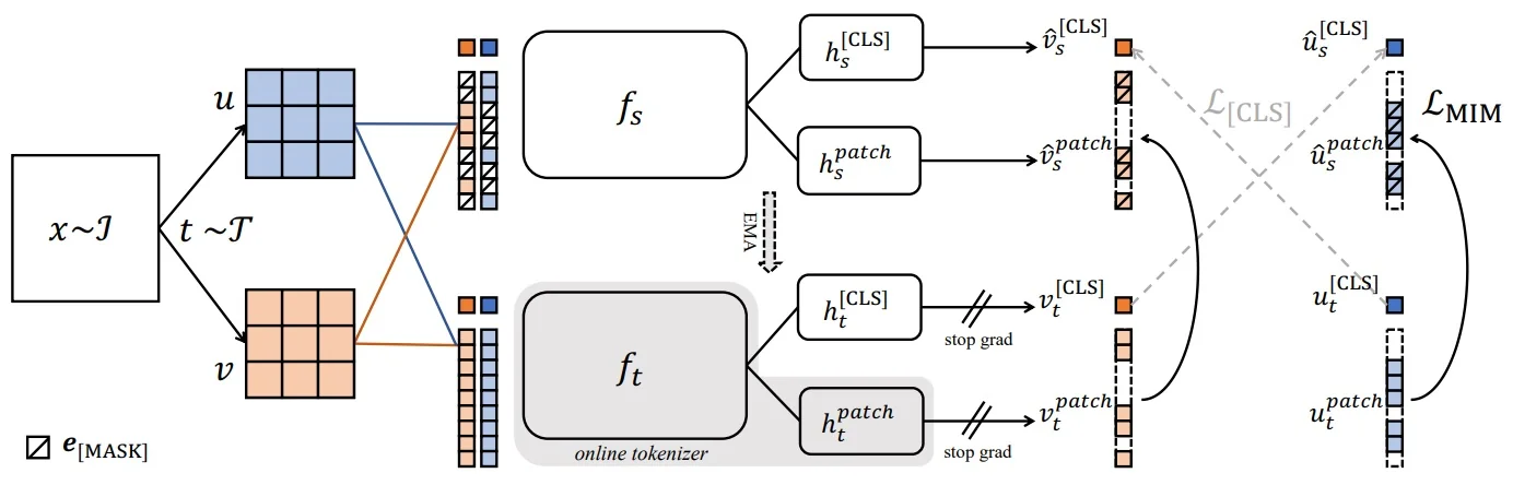
The iBOT architecture, illustrated in Figure 22.54, unifies the scalability of masked autoencoders with the semantic alignment of self-distillation. It adopts an asymmetric student–teacher framework where both networks are Vision Transformers (ViTs), but operate on distinct inputs and follow different training dynamics. Specifically, the student receives a randomly masked view of the image, while the teacher always processes the full, unmasked version. This input-level asymmetry, inspired by masked autoencoders like MAE, encourages the student to infer semantically meaningful content from limited context.
Beyond masking, iBOT incorporates several training asymmetries central to the success of DINO. The teacher network is updated as an exponential moving average (EMA) of the student’s parameters, making it a slowly evolving target that stabilizes learning. A stop-gradient is applied to the teacher’s output to prevent gradient flow during loss computation. Crucially, iBOT also employs two additional mechanisms to avoid representational collapse: centering, which subtracts a running mean from the teacher’s output to encourage diversity, and sharpening, which applies a low temperature to the teacher’s softmax to yield confident, discriminative targets. These mechanisms are applied not only to the global [CLS] token (as in DINO), but also extended to patch-level outputs for masked tokens.
Together, these architectural and training asymmetries allow iBOT to reinterpret masked image modeling as a feature-level distillation task—eschewing pixel-level reconstruction in favor of predicting the teacher’s semantic output distributions. This reframing produces linearly separable features suitable for frozen transfer and forms the conceptual foundation upon which DINOv2 is built.
An input image of size \(224 \times 224\) is tokenized into a grid of non-overlapping \(16 \times 16\) patches, producing 196 visual tokens. A learnable [CLS] token is prepended, resulting in a sequence of \(N = 197\) tokens. Each token is projected into a high-dimensional embedding (e.g., \(D = 768\) for ViT-B) and augmented with fixed sine-cosine positional encodings.
The student network receives a corrupted version of this sequence, where a large random subset (e.g., 75%) of patch tokens is replaced by a shared learned [MASK] token. The student processes the masked sequence and outputs embeddings for all tokens—both visible and masked—including the [CLS] token. These are passed through a shared projection head to produce probability distributions over a fixed vocabulary of prototypes (typically \(K = 8192\)), one per token.
The teacher network, updated via exponential moving average (EMA) from the student, processes the full, unmasked sequence of the same image. It outputs target distributions for both the patch tokens and the global [CLS] token. These soft targets act as an online tokenizer, dynamically adapting over training and eliminating the need for discrete codebooks or external pretraining (as used in BEiT).
Learning is driven by matching the student’s predictions to the teacher’s targets at two levels:
- Patch-level distillation: The student predicts the teacher’s soft feature distributions for masked patches using a cross-entropy loss. This encourages localized, context-aware feature learning.
- Global self-distillation: The student’s [CLS] token—typically from a different augmented view—is aligned with the teacher’s [CLS] token, following the DINO objective. This enforces global semantic consistency.
This dual prediction setup introduces two key advantages over pixel-based masked modeling:
- Latent-space supervision: iBOT operates entirely in a learned semantic space, avoiding the ambiguity of pixel regression and focusing instead on high-level structure.
- Unified local and global alignment: By combining patch-level and image-level objectives, iBOT learns both part-based semantics and holistic representations in a single pass.
These innovations yield high-quality, linearly separable features even without fine-tuning—resolving a key shortcoming of MAE. Rather than preserving MAE’s encoder–decoder architecture, iBOT retains its token-masking formulation while introducing semantic supervision through a symmetric, DINO-inspired self-distillation design. In this way, iBOT serves as a conceptual and algorithmic bridge to DINOv2. In the next part, we formalize the iBOT objective and detail the mechanisms that ensure effective alignment across masked tokens and global embeddings.
iBOT Loss Function and Self-Distillation Objective The iBOT framework introduces a unified self-supervised learning objective that combines masked image modeling (MIM) with cross-view self-distillation. The two components work in tandem to supervise the model at both local (patch-level) and global (image-level) scales, without requiring class labels or reconstruction targets.
Patch-Level Loss: Masked Image Modeling as Feature Distillation. Let \( u \) and \( v \) be two augmented views of an image \( x \). The student network \( f_s \circ h_s \) receives masked views \( \hat {u} \), \( \hat {v} \), where a random subset of patch tokens is replaced by a shared, learnable token embedding \( e^{\mbox{mask}} \). The teacher network \( f_t \circ h_t \), updated via exponential moving average (EMA), always observes the unmasked views.
Each network maps patch tokens to a probability distribution over \( K \) learnable prototypes. These prototypes are not semantic classes, but rather serve as anchors in the representation space, following the idea introduced in DINO [70]: by applying a softmax over the dot products between features and prototype vectors, the model is effectively solving an unsupervised classification task it defines for itself. This encourages separation and clustering of features into emergent categories.
Let \( P_{\theta }^{\mbox{patch}}(\hat {u}) = \hat {u}_s^{\mbox{patch}} \in \mathbb {R}^{N \times K} \) be the student’s patch-level output for the masked view \( \hat {u} \), and \( P_{\theta '}^{\mbox{patch}}(u) = u_t^{\mbox{patch}} \in \mathbb {R}^{N \times K} \) the teacher’s output on the corresponding full view \( u \), where \( N \) is the number of patches. The mask indicator \( m_i \in \{0,1\} \) specifies which positions were masked.
The patch-level masked image modeling loss for view \( u \) is then computed as a masked cross-entropy: \[ \mathcal {L}_{\mbox{MIM}}^{(u)} = -\sum _{i=1}^N m_i \cdot P_{\theta '}^{\mbox{patch}}(u_i)^\top \log P_{\theta }^{\mbox{patch}}(\hat {u}_i) \] This encourages the student to match the teacher’s soft probability distribution at each masked patch, thereby learning semantically grounded, context-aware features. Cross-entropy penalizes discrepancies between the teacher’s soft target (a sharpened, semantically meaningful distribution) and the student’s prediction. Unlike one-hot targets, this soft supervision enables smooth gradients and richer learning signals.
An identical loss \( \mathcal {L}_{\mbox{MIM}}^{(v)} \) is computed between \( P_{\theta '}^{\mbox{patch}}(v) \) and \( P_{\theta }^{\mbox{patch}}(\hat {v}) \), and the final patch-level loss is symmetrized: \[ \mathcal {L}_{\mbox{MIM}} = \frac {1}{2} \left ( \mathcal {L}_{\mbox{MIM}}^{(u)} + \mathcal {L}_{\mbox{MIM}}^{(v)} \right ) \] This ensures that both views contribute equally, improving generalization across diverse augmentations.
Global Loss: Cross-View [CLS] Token Distillation. In parallel, iBOT minimizes a self-distillation loss between [CLS] tokens from opposite views. The teacher processes full inputs \( u \), \( v \) to yield \( u_t^{[\mbox{CLS}]} \), \( v_t^{[\mbox{CLS}]} \), while the student processes masked inputs \( \hat {v} \), \( \hat {u} \) to produce \( \hat {v}_s^{[\mbox{CLS}]} \), \( \hat {u}_s^{[\mbox{CLS}]} \). The cross-entropy loss is: \[ \mathcal {L}_{\mbox{CLS}} = -\frac {1}{2} \left ( P_{\theta '}^{[\mbox{CLS}]}(u)^\top \log P_{\theta }^{[\mbox{CLS}]}(\hat {v}) + P_{\theta '}^{[\mbox{CLS}]}(v)^\top \log P_{\theta }^{[\mbox{CLS}]}(\hat {u}) \right ) \]
Final Objective. The total loss is the sum of local (patch) and global ([CLS]) distillation objectives: \[ \mathcal {L}_{\mbox{iBOT}} = \mathcal {L}_{\mbox{MIM}} + \mathcal {L}_{\mbox{CLS}} \]
Centering and Sharpening for Stability. To prevent representation collapse and promote meaningful feature diversity, iBOT adopts two output normalization techniques—centering and sharpening—originally introduced in DINO [70]. These operations are applied exclusively to the teacher network’s logits prior to the softmax, introducing an essential asymmetry between the teacher and student distributions.
- Centering: Let \( \mathbf {z} \) denote the teacher’s raw pre-softmax logits for either patch tokens or [CLS] tokens. A running exponential moving average (EMA) of the logits is maintained across training steps to compute a global center vector \( \mathbf {c} \in \mathbb {R}^K \). For each mini-batch, the logits are centered as: \[ \mathbf {z}_{\mbox{centered}} = \mathbf {z} - \mathbf {c}, \quad \mbox{where} \quad \mathbf {c} \leftarrow m' \cdot \mathbf {c} + (1 - m') \cdot \mbox{mean}_{\mbox{batch}}(\mathbf {z}) \] The momentum coefficient \( m' \in [0,1) \) controls the update smoothness. Centering ensures that all prototype dimensions remain active and prevents output collapse to a degenerate solution where one prototype dominates.
- Sharpening: The centered logits are divided by a low temperature \( \tau _t \ll 1 \), which flattens the softmax denominator and yields a more peaked probability distribution: \[ P_{\theta '}(x) = \mbox{softmax}\left ( \frac {x - \mathbf {c}}{\tau _t} \right ), \quad P_{\theta }(x) = \mbox{softmax}\left ( \frac {x}{\tau _s} \right ) \] The student temperature \( \tau _s \) is typically set to a higher value (e.g., \( \tau _s = 0.1 \)) than the teacher temperature (e.g., \( \tau _t = 0.04 \)), further accentuating the asymmetry between the two outputs.
This teacher–student temperature asymmetry serves multiple purposes. First, it provides a stronger and less noisy supervision signal by making the teacher’s output distribution highly confident (i.e., close to one-hot), which simplifies the student’s task of matching it. Second, it prevents representational uniformity by preserving inter-sample diversity: the teacher maintains sharp, discriminative distributions, while the student must learn to approximate them despite incomplete input views and higher entropy outputs.
Together, centering and sharpening constitute a critical design choice in iBOT. The use of batch-wise statistics (for centering) and low-temperature scaling (for sharpening) ensures that the learned token distributions remain diverse, stable, and semantically structured across the training trajectory.
These mechanisms operate as a form of entropy regularization and are essential to achieving effective self-distillation without collapse.
Projection Head Sharing. Finally, iBOT shares the projection head between [CLS] and patch tokens: \[ h_s^{[\mbox{CLS}]} = h_s^{\mbox{patch}}, \quad h_t^{[\mbox{CLS}]} = h_t^{\mbox{patch}} \] This enforces alignment in the learned representation space and improves transfer performance by promoting consistency between local and global features.
Together, these components allow iBOT to reinterpret masked image modeling as feature-level knowledge distillation with semantically rich, soft supervision—bridging the scalability of MAE with the semantic structure of DINO.
iBOT Training Procedure The full iBOT training procedure is summarized in the following PyTorch-style pseudocode.
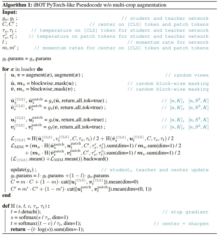
This training loop operationalizes the central innovations of iBOT: online semantic tokenization via the teacher, joint learning of local and global targets, and distribution-level alignment using cross-entropy in a stabilized feature space. These design decisions form the foundation upon which iBOT outperforms prior methods in both semantic classification and dense vision tasks. We now turn to its empirical evaluation.
Empirical Results and Evaluation iBOT demonstrates state-of-the-art performance across a wide range of self-supervised benchmarks, successfully bridging the gap between generative and contrastive/distillation-based methods. Its dual-level objective—combining a local, patch-level masked prediction task with a global [CLS] token self-distillation task—produces representations that are highly linearly separable and semantically structured, even without fine-tuning.
ImageNet Linear Probing: A key weakness of earlier masked image models such as BEiT and MAE was their poor performance under linear probing, due to their focus on pixel-level reconstruction rather than semantic separability. As shown in the below table, iBOT decisively resolves this issue. Using a ViT-B/16 backbone, iBOT achieves a linear probing accuracy of 79.5% on ImageNet, outperforming both the generative BEiT and the distillation-based DINO. This result confirms that iBOT’s features are not just powerful but also organized in a way that is directly usable for downstream classification without further adaptation.
| Method | Arch. | Epochs | Linear (%) | Fine-tune (%) |
|---|---|---|---|---|
| DINO | ViT-B/16 | 1600 | 78.2 | 83.6 |
| BEiT | ViT-B/16 | 800 | 71.7 | 83.4 |
| iBOT | ViT-B/16 | 1600 | 79.5 | 84.0 |
Label-Efficient Transfer: iBOT also excels in low-label regimes, demonstrating high sample efficiency. On semi-supervised benchmarks using only 1% or 10% of ImageNet labels, it consistently outperforms DINO using the same ViT-S/16 backbone. This suggests that iBOT’s representations capture class-relevant structure so effectively that a linear classifier can succeed with minimal supervision.
| Method | Arch. | 1% | 10% |
|---|---|---|---|
| DINO | ViT-S/16 | 60.3 | 74.3 |
| iBOT | ViT-S/16 | 61.9 | 75.1 |
Unsupervised Clustering: The benefit of iBOT’s patch-level distillation is particularly evident in clustering tasks. Without access to any labels, iBOT achieves superior performance over DINO on all standard clustering metrics. The additional supervision on masked tokens encourages the model to develop finer-grained visual representations that enhance semantic separation across classes.
| Method | Arch. | ACC | ARI | NMI | FMI |
|---|---|---|---|---|---|
| DINO | ViT-S/16 | 41.4 | 29.8 | 76.8 | 32.8 |
| iBOT | ViT-S/16 | 43.4 | 32.8 | 78.6 | 35.6 |
Downstream Transfer: Detection and Dense Prediction. iBOT generalizes effectively across a wide spectrum of vision tasks. The table below presents results on object detection and instance segmentation (COCO dataset, evaluated via AP metrics), as well as semantic segmentation (ADE20K, measured by mIoU). While object detection involves sparse localization of individual objects, both instance and semantic segmentation require dense, per-pixel predictions. By jointly supervising both global [CLS] and patch-level token features, iBOT fuses DINO’s semantic abstraction with MAE’s spatial precision—resulting in superior performance across both sparse and dense modalities.
| Method | AP\(^{\mbox{box}}\) | AP\(^{\mbox{mask}}\) | mIoU (ADE) |
| BEiT | 50.1 | 43.5 | 45.8 |
| DINO | 50.1 | 43.4 | 46.8 |
| iBOT | 51.2 | 44.2 | 50.0 |
Summary: These results demonstrate that iBOT’s hybrid design—combining masked image modeling with self-distillation—yields representations that are not only semantically rich but also spatially precise. Unlike MAE, which primarily excels at reconstruction, iBOT produces features that are linearly separable and transferable across diverse downstream tasks, even without extensive fine-tuning. This unification of global and local supervision makes iBOT a crucial stepping stone toward more general and scalable vision frameworks such as DINOv2.
Ablation Studies and Component Analysis To understand which components of iBOT contribute most to its empirical success, the authors conducted a series of ablation studies. These isolate the effects of patch-level losses, projection head configurations, masking strategies, and temperature stabilization mechanisms. The results highlight the architectural decisions critical for learning linearly separable, transferable features.
Effect of the Masked Token Prediction Loss. The patch-level masked image modeling (MIM) loss is a defining element of iBOT’s design. The following table shows that removing this term leads to a sharp drop in linear probing performance (from 79.5% to 75.3%), confirming that token-level supervision provides essential fine-grained semantic guidance beyond global alignment.
| Loss Components | Linear (%) | Fine-tune (%) |
|---|---|---|
| Global + Patch (Full iBOT) | 79.5 | 84.0 |
| Global only ([CLS] distill) | 75.3 | 83.3 |
Shared vs. Separate Projection Heads. iBOT employs a single projection head shared across both patch tokens and the global [CLS] token. The following table shows that using separate heads yields negligible improvement in fine-tune, and a slight decrease in linear probing, and it introduces additional complexity. Therefore, the shared configuration simplifies training and generalization without loss of accuracy.
| Head Configuration | Linear (%) | Fine-tune (%) |
|---|---|---|
| Shared Head (default) | 79.5 | 84.0 |
| Separate Heads | 79.4 | 84.1 |
Masking Strategy. Although iBOT [819] briefly mentions blockwise masking, its actual implementation employs a random masking strategy. For each image, either no masking is applied (50% probability), enabling pure [CLS] supervision, or a prediction ratio is uniformly sampled from the range \([0.1, 0.5]\) and used to randomly mask patches. This dynamic approach, unlike MAE’s fixed 75% masking or BEiT’s structured blockwise strategy, stabilizes training under multi-crop augmentation and balances local and global supervision.
Temperature Sensitivity and Centering. As in DINO, iBOT employs sharpening (low-temperature softmax) and centering for both global and patch tokens. Teacher temperatures of 0.04 and momentum-updated running means improve contrastiveness and prevent representational collapse. These mechanisms are essential for balanced distributional supervision in both prediction streams.
Summary. These ablations demonstrate that iBOT’s strong transfer performance arises from a precise combination of design choices: patch-level distillation, architectural parameter sharing, structured masking, and symmetric stabilization. These components collectively reinforce the model’s ability to align semantic content across masked and unmasked views, foreshadowing key techniques later adopted in DINOv2.
iBOT vs. DINO: Paving the Way for DINOv2 While iBOT is a direct descendant of DINO, sharing its student–teacher architecture and self-distillation principles, it introduces a pivotal extension. DINO enforces consistency between the global [CLS] tokens produced by different views of the same image, aligning them in feature space via a cross-entropy loss. iBOT generalizes this strategy by extending the distillation target to all masked patch tokens using a masked image modeling (MIM) loss. This addition allows iBOT to learn not only holistic image-level semantics, but also fine-grained local features across hundreds of spatial tokens. Both models rely on similar strong augmentation pipelines, including multi-crop views, to provide diverse training signals.
In this way, iBOT can be understood as a superset of DINO. It retains the original [CLS]-based objective of DINO, while augmenting it with a patch-level prediction task that enables richer spatial understanding. This hybrid formulation proves especially effective for transfer to dense prediction tasks, such as object detection and semantic segmentation, where local features are critical.
From iBOT to DINOv2. DINOv2 keeps iBOT’s dual–loss recipe—global [CLS]–level and local patch–level self-distillation—yet adds a small set of focused upgrades that make the framework scale stably to hundreds of millions of images and billions of parameters:
- KoLeo Regularizer: a \(k\)-NN entropy term on the [CLS] embedding flattens the batch feature distribution, preventing collapse and boosting instance–retrieval accuracy.
- Sinkhorn–Knopp Centering [72]: the teacher logits are re-centered with a few SK iterations rather than a simple centering + sharpening. This enforces balanced prototype usage and further stabilises training.
- Untied Projection Heads: in contrast to iBOT’s single shared head—which the authors of iBOT showed was best at their scale—DINOv2 allocates separate MLPs to the global and local branches. Decoupling allows the [CLS] head to specialise in semantic alignment while the patch head captures spatial detail, yielding consistent gains once model and data are scaled up.
- Multi-Crop Optimisations: positional embeddings are interpolated on-the-fly to support the usual mix of \(224^2\) and \(98^2\) crops, and training ends with a short high-resolution phase (\(518^2\)) using the “FixRes” trick to sharpen pixel-level features without incurring full-resolution cost.
- LVD-142M Corpus: a deduplicated 142-M image collection supplies the scale and diversity that earlier ImageNet-based training lacked, reducing reliance on heavy augmentations and improving cross-domain transfer.
- Efficiency Tweaks: FlashAttention, sequence packing (masking attention across crops), compute-skipping stochastic depth, FSDP, and knowledge-distillation pre-warming all reduce memory usage and training time. Crucially, these improvements enable the use of larger batch sizes, which in turn sharpen the statistical stability of prototype assignments and improve probing accuracy. This leads to stronger, more linearly separable features—often usable off the shelf without finetuning.
Collectively, the KoLeo regularizer, Sinkhorn–Knopp (SK) centering, and untied projection heads address the core pitfalls of self-distillation: feature collapse, prototype imbalance, and representational bottlenecks. When combined with large-scale data (LVD-142M), high-resolution finetuning, and a suite of efficiency optimizations (e.g., FlashAttention, stochastic depth, sequence packing), these changes enable DINOv2 to scale gracefully and achieve state-of-the-art performance in frozen, linear, and low-shot settings—often surpassing supervised ViTs of similar size.
While many of these upgrades build on familiar components—KoLeo from SSCD, dual-loss from iBOT, and data curation from prior work—DINOv2 introduces a novel centering scheme based on the Sinkhorn–Knopp algorithm. As the only mechanism not previously covered in this chapter, it forms the focus of the next part. We then proceed to summarize DINOv2’s empirical results and ablations.
Sinkhorn–Knopp Centering in DINOv2 In self-distillation frameworks like DINOv2, the teacher assigns each image a soft probability distribution over \( K \) learned prototypes. However, if these assignments become too concentrated—e.g., most images are mapped to a small subset of prototypes—the model risks representational collapse: features lose diversity, and learning stagnates. This imbalance is especially problematic in large-scale settings, where uniform usage of model capacity is critical.
Intuition. The goal of centering in DINOv2 is to ensure that:
- 1.
- No prototype dominates the batch—each prototype is used roughly equally.
- 2.
- Each image maintains uncertainty—its assignment is not overly confident.
In other words, we want a batch-level distribution of prototype assignments that is balanced and high-entropy. Such diversity prevents collapse and improves representation learning. While DINO and iBOT achieved this by subtracting an EMA-based center and applying sharpening, DINOv2 adopts a more principled, batch-local alternative: Sinkhorn–Knopp normalization.
Sinkhorn–Knopp Algorithm. Let \( z \in \mathbb {R}^{K \times B} \) denote the teacher’s logits assigning \( B \) image features to \( K \) learned prototypes. DINOv2 transforms these raw logits into a soft, balanced assignment matrix \( Q \in \mathbb {R}^{K \times B} \) as follows:
Step 1: Affinity Matrix Construction. The teacher’s logits \( z \in \mathbb {R}^{K \times B} \), which measure the similarity between each image and prototype, are sharpened by a temperature parameter \( \tau > 0 \) and exponentiated to form the affinity matrix \( A \): \[ A_{ij} = \exp \left (\frac {z_{ij}}{\tau }\right ). \] This transformation amplifies high-confidence predictions when \( \tau \) is small, making the matrix entries more peaked. However, it is important to emphasize that this is not a softmax: unlike softmax, the rows (or columns) of \( A \) are not normalized to sum to one. As such, \( A \in \mathbb {R}_{+}^{K \times B} \) contains unnormalized, non-negative scores reflecting the raw affinity between images and prototypes.
Why is this distinction important? A softmax would normalize over one axis—typically columns—causing the output to behave like a probability distribution for each sample. But this ignores the balance across prototypes: some prototypes might dominate the entire batch if their logits are consistently high. This can lead to prototype collapse, where only a few prototypes are used during training.
Step 2: Sinkhorn–Knopp Rescaling. To transform the unnormalized affinity matrix \( A \in \mathbb {R}_{+}^{K \times B} \) into a balanced assignment matrix \( Q \), DINOv2 applies the Sinkhorn–Knopp algorithm, which rescales both rows and columns to enforce specific marginal constraints: \[ Q = \operatorname {diag}(u)\, A\, \operatorname {diag}(v), \] where \( u \in \mathbb {R}^{K}_{> 0} \) and \( v \in \mathbb {R}^{B}_{> 0} \) are scaling vectors, and \( \operatorname {diag}(\cdot ) \) constructs a diagonal matrix from its argument.
This transformation adjusts:
- Rows: Multiplication by \( \operatorname {diag}(u) \) on the left scales each row \( i \) of \( A \) by \( u_i \),
- Columns: Multiplication by \( \operatorname {diag}(v) \) on the right scales each column \( j \) of \( A \) by \( v_j \).
The effect is to redistribute the raw affinity mass in \( A \), without altering the internal ranking of logits within each row or column. The goal is to find \( u \) and \( v \) such that the resulting matrix \( Q \) satisfies the desired marginal constraints: \[ Q \mathbf {1}_B = \tfrac {1}{K} \mathbf {1}_K \quad \mbox{(equal total mass per prototype)}, \qquad Q^\top \mathbf {1}_K = \mathbf {1}_B \quad \mbox{(valid distribution per image)}. \]
How the Rescaling Works. Rather than solving these coupled equations for \( u \) and \( v \) in closed form, the Sinkhorn–Knopp algorithm computes them through fixed-point iteration: \begin {align*} \text {initialize:} \quad & u^{(0)} = \tfrac {1}{K} \mathbf {1}_K, \quad v^{(0)} = \mathbf {1}_B, \\ \text {repeat:} \quad & v^{(t+1)} = \left ( A^\top u^{(t)} \right )^{-1}, \\ & u^{(t+1)} = \left ( A v^{(t+1)} \right )^{-1} \cdot \tfrac {1}{K}, \end {align*}
where division and inversion are element-wise. Each update enforces one marginal exactly while slightly perturbing the other. Despite this tug-of-war, the process converges rapidly: after only 3–5 iterations, the residual marginal error is negligible (typically \( < 10^{-3} \)).
Why This Works. The final matrix \( Q = \operatorname {diag}(u)\,A\,\operatorname {diag}(v) \) preserves the shape and non-negativity of \( A \), but scales it such that:
- Each prototype receives the same total assignment mass across the batch (row-balanced),
- Each sample’s assignment forms a valid probability distribution (column-normalized).
This procedure is differentiable, stateless, and highly parallelizable.
Sinkhorn–Knopp Algorithm (NumPy Pseudocode) The Sinkhorn–Knopp algorithm transforms an unnormalized affinity matrix \( A \in \mathbb {R}^{K \times B} \) into a balanced assignment matrix \( Q \) that satisfies:
- Column-normalization: Each sample is softly assigned, so each column sums to 1.
- Row-equipartition: Each prototype is used equally across the batch, so each row sums to \( \tfrac {1}{K} \).
This is accomplished by solving for scaling vectors \( u \in \mathbb {R}^K \) and \( v \in \mathbb {R}^B \) such that: \[ Q = \operatorname {diag}(u) \cdot A \cdot \operatorname {diag}(v), \] with updates alternating between enforcing row and column constraints.
import numpy as np


def sinkhorn_knopp(logits: np.ndarray,
                   tau: float = 0.05,
                   n_iter: int = 3,
                   eps: float = 1e-9) -> np.ndarray:
    """
    Sinkhorn-Knopp matrix balancing for prototype assignments.

    Args:
    logits : (K, B) teacher logits (K = prototypes, B = samples)
    tau    : temperature for sharpening (smaller -> peakier)
    n_iter : number of Sinkhorn iterations (3{5 usually sufficient)
    eps    : small constant for numerical stability

    Returns:
    Q : (K, B) assignment matrix with row sums approx 1/K
    and column sums approx 1
    """
    K, B = logits.shape

    # Step 1: Compute affinity matrix A (unnormalized)
    A = np.exp(logits / tau)

    # Step 2: Initialize scaling vectors
    u = np.ones((K, 1), dtype=A.dtype) / K  # target row mass
    v = np.ones((B, 1), dtype=A.dtype)      # target column mass

    # Step 3: Iterative normalization
    for _ in range(n_iter):
        v = 1.0 / (A.T @ u + eps)         # column update (per sample)
        u = (1.0 / K) / (A @ v + eps)     # row update (equipartition)

    # Step 4: Reconstruct Q = diag(u) @ A @ diag(v)
    Q = (u * A) * v.T                     # NumPy broadcasting

    # Optional: normalize Q to sum to 1
    Q /= Q.sum()

    return Q
Explanation and DINOv2 Motivation
- Step 1: Affinity Construction. The teacher logits are sharpened by temperature \( \tau \) and exponentiated. This yields \( A \in \mathbb {R}^{K \times B} \), where \( A_{ij} = \exp (z_{ij} / \tau ) \) encodes prototype–sample affinity. Unlike softmax, this does not normalize across rows or columns.
- Step 2: Scaling Initialization. Vectors \( u \) and \( v \) are initialized to match the target row and column marginals. In DINOv2, rows should sum to \( \tfrac {1}{K} \) (equal prototype usage), while columns should sum to 1 (each image is fully assigned).
- Step 3: Iterative Balancing. Updates alternate: \[ v = \frac {1}{A^\top u + \varepsilon }, \qquad u = \frac {1/K}{A v + \varepsilon }, \] which adjusts \( v \) to ensure column sums equal 1 and \( u \) to enforce row sums of \( \tfrac {1}{K} \). The process converges quickly (3–5 steps suffice).
- Step 4: Matrix Scaling. The final assignment matrix \( Q = \operatorname {diag}(u) \cdot A \cdot \operatorname {diag}(v) \) is assembled once the updates converge. NumPy’s broadcasting handles this efficiently via (u * A) * v.T.
This doubly-normalized structure prevents prototype collapse by guaranteeing uniform prototype participation and valid image-level supervision. Unlike EMA centering, this method is purely batch-local, stateless, and fully differentiable—making it ideal for large-scale training as used in DINOv2.
Toy Example: The Fair Project Manager To build intuition for Sinkhorn–Knopp centering, consider a project manager assigning tasks to a team of specialized workers. This mirrors the self-supervised assignment problem in DINOv2: allocating image embeddings (tasks) to prototype vectors (workers) in a fair, balanced manner. Without proper constraints, greedy matching might overload generalists and underuse specialists—leading to the very collapse Sinkhorn centering aims to prevent.
The Scenario. We have \( K = 3 \) workers:
- Alice (A): a frontend design expert.
- Bob (B): a backend logic specialist.
- Charlie (C): a versatile full-stack generalist.
A batch of \( B = 4 \) tasks arrives:
- T1: Create UI Mockup.
- T2: Implement Database API.
- T3: Debug Login Flow (mixed).
- T4: Refactor CSS.
Raw Affinity Scores. The manager scores how well each worker fits each task, producing an unnormalized affinity matrix \( A \in \mathbb {R}^{3 \times 4} \): \[ A = \begin {bmatrix} 10 & 1 & 5 & 9 \\ 1 & 10 & 6 & 1 \\ 7 & 8 & 9 & 8 \\ \end {bmatrix}. \] Rows index workers and columns index tasks; a higher value indicates stronger compatibility. For example, Alice is well-suited for frontend-related tasks (T1, T4), Bob excels at backend (T2), and Charlie scores decently across the board.
The Problem. A naive greedy assignment—giving each task to the worker with the highest score—would result in Charlie taking most tasks, starving Alice and Bob of work. This is analogous to prototype collapse, where only a few prototypes are responsible for most of the supervision signal, degrading representational diversity.
The Goal. We want a soft assignment matrix \( Q \in \mathbb {R}^{3 \times 4} \) such that:
- Every task is fully assigned: Each column sums to 1.
- Every worker gets equal load: Each row sums to \( \tfrac {4}{3} \) (i.e., 4 tasks divided equally among 3 workers).
Such a matrix is approximately doubly stochastic, but scaled to reflect our desired marginals.
Applying Sinkhorn–Knopp Centering. The algorithm proceeds in three main steps:
- 1.
- Sharpen the affinities using a temperature \( \tau \), and exponentiate: \[ K = \exp \left (\frac {A}{\tau }\right ). \]
- 2.
- Initialize row and column scaling vectors \( u \in \mathbb {R}^3 \), \( v \in \mathbb {R}^4 \).
- 3.
- Alternate normalization: \begin {align*} v &\leftarrow \frac {1}{K^\top u + \varepsilon } \quad \text {(normalize columns)} \\ u &\leftarrow \frac {1/3}{K v + \varepsilon } \quad \text {(normalize rows)} \end {align*}
After a few iterations, the result converges to: \[ Q = \operatorname {diag}(u) \cdot K \cdot \operatorname {diag}(v). \]
Result. A typical output might be: \[ Q \approx \begin {bmatrix} 0.60 & 0.13 & 0.15 & 0.45 \\ 0.10 & 0.70 & 0.33 & 0.20 \\ 0.30 & 0.17 & 0.52 & 0.35 \\ \end {bmatrix}, \quad \mbox{row sums} \approx 1.33, \quad \mbox{column sums} = 1. \] This matrix shows that:
- Alice receives most of T1 and T4 (frontend).
- Bob dominates T2 (backend).
- Charlie helps with all tasks, especially the mixed T3.
Each worker handles \( \approx \tfrac {4}{3} \) tasks in total, and every task is fully distributed.
Why This Works. The Sinkhorn solution ensures:
- Every task is covered: All task columns sum to 1.
- No one is overloaded: Row sums are balanced across workers.
- Preferences are respected: Assignments remain proportional to the original affinities.
It yields the most unbiased, entropy-regularized allocation compatible with both local preferences and global fairness constraints.
Connection to DINOv2 This fair allocation scenario maps directly onto the representation learning setup in DINOv2. Each part of the toy example has a precise analogue in the self-supervised learning framework:
- Workers \( \rightarrow \) Prototypes — learnable vectors representing semantic regions of feature space.
- Tasks \( \rightarrow \) Image embeddings — typically the [CLS] token of a Vision Transformer computed from each image in the batch.
- Affinity scores \( A \rightarrow \) Teacher logits — dot products between teacher embeddings and prototypes, representing how well each image matches each prototype.
- Assignment matrix \( Q \rightarrow \) Soft targets — the balanced probability distributions used to supervise the student network.
In the original DINO framework, each image embedding is treated independently: the teacher logits for each image are normalized via a softmax, yielding a local assignment distribution. While simple, this can lead to prototype collapse—where only a few generic prototypes are favored and others are ignored, similar to always assigning tasks to a single overqualified worker (like Charlie).
DINOv2 replaces this with a global, batch-wise assignment using the Sinkhorn–Knopp algorithm. Instead of computing a distribution per image in isolation, it operates on the entire \( K \times B \) matrix of teacher logits—where \( K \) is the number of prototypes and \( B \) the batch size.
The Sinkhorn iterations compute scaling vectors \( u \) and \( v \) such that the resulting matrix \[ Q = \operatorname {diag}(u) \cdot \exp \left ( \frac {A}{\tau } \right ) \cdot \operatorname {diag}(v) \] satisfies two critical constraints:
- Column-normalization: Each image embedding (typically the [CLS] token) is assigned to all prototypes via a soft probability distribution whose entries sum to 1. This ensures that each image produces a valid supervision signal, and that no supervision mass is lost or duplicated.
- Row-equipartition: Each prototype receives exactly \( \tfrac {1}{K} \) of the total assignment mass, enforcing that prototypes are used evenly across the batch—preventing collapse and encouraging specialization.
Just like the project manager who must assign tasks while ensuring each worker gets a fair workload and each task is fully handled, DINOv2 uses Sinkhorn centering to jointly optimize assignment quality and diversity. This global balancing acts as a regularizer that improves coverage of the feature space, stabilizes training at scale, and encourages the emergence of rich, semantically structured representations—all without introducing momentum encoders or memory banks.
In summary, Sinkhorn centering is DINOv2’s principled solution to the core problem of contrastive self-supervision: how to prevent shortcut solutions (like assigning all images to a few dominant prototypes) while still respecting the structure learned from the teacher network’s representations.
Linear Evaluation on ImageNet and Comparison to Prior Work To evaluate the representational strength of DINOv2, the authors conduct a standard linear evaluation on ImageNet-1k using frozen pretrained features. The following table compares DINOv2 to prior self-supervised and weakly supervised methods under consistent resolution and evaluation settings. Each model is trained using its respective backbone and dataset, without finetuning.
DINOv2 achieves state-of-the-art top-1 accuracy among self-supervised methods across all model scales. Notably, a ViT-g/14 pretrained with DINOv2 on LVD-142M achieves 86.5% top-1 accuracy with a linear classifier and 83.5% with a \(k\)-NN classifier—surpassing earlier methods such as iBOT, MAE, and even some large-scale weakly supervised models like OpenCLIP and SWAG.
| Method | Architecture | Data | Text Sup. | \(k\)-NN (%) | Linear (%) | ReaL (%) |
|---|---|---|---|---|---|---|
Weakly Supervised |
||||||
| CLIP | ViT-L/14 | WIT-400M | ✓ | 79.8 | 84.3 | 88.1 |
| CLIP | ViT-L/14\(^{336}\) | WIT-400M | ✓ | 80.5 | 85.3 | 88.8 |
| SWAG | ViT-H/14 | IG-3.6B | ✓ | 82.6 | 85.7 | 88.7 |
| OpenCLIP | ViT-H/14 | LAION-2B | ✓ | 81.7 | 84.4 | 88.4 |
| OpenCLIP | ViT-G/14 | LAION-2B | ✓ | 83.2 | 86.2 | 89.4 |
| EVA-CLIP | ViT-g/14 | custom* | ✓ | 83.5 | 86.4 | 89.3 |
Self-Supervised |
||||||
| MAE | ViT-H/14 | INet-1k | ✗ | 49.4 | 76.6 | 83.3 |
| DINO | ViT-S/8 | INet-1k | ✗ | 78.6 | 79.2 | 85.5 |
| MSN | ViT-L/7 | INet-1k | ✗ | 79.2 | 80.7 | 86.0 |
| EsViT | Swin-B/W14 | INet-1k | ✗ | 79.4 | 81.3 | 87.0 |
| Mugs | ViT-L/16 | INet-1k | ✗ | 80.2 | 82.1 | 86.9 |
| iBOT | ViT-L/16 | INet-22k | ✗ | 72.9 | 82.3 | 87.5 |
| DINOv2 | ViT-S/14 | LVD-142M | ✗ | 79.0 | 81.1 | 86.6 |
| DINOv2 | ViT-B/14 | LVD-142M | ✗ | 82.1 | 84.5 | 88.3 |
| DINOv2 | ViT-L/14 | LVD-142M | ✗ | 83.5 | 86.3 | 89.5 |
| DINOv2 | ViT-g/14 | LVD-142M | ✗ | 83.5 | 86.5 | 89.6 |
We can clearly see that the combination of patch-level and global objectives, along with improvements such as the KoLeo regularizer, Sinkhorn-normalized teacher outputs, and a large curated training corpus (LVD-142M), enables DINOv2 to match or exceed the performance of prior self-supervised methods—especially in frozen, plug-and-play transfer setups.
Ablation of Design Modifications from iBOT to DINOv2 To better understand which architectural and training refinements most contributed to DINOv2’s performance, the authors conducted a controlled ablation starting from the iBOT baseline. Each row in the following table reflects the incremental addition of a component, measuring its effect on frozen \(k\)-NN and linear probe accuracy using a ViT-L/14 backbone pretrained on ImageNet-22k. These experiments were run under equal compute budgets and consistent evaluation settings.
| Modification | \(k\)-NN (%) | Linear (%) |
|---|---|---|
| iBOT baseline | 72.9 | 82.3 |
| + Our reproduction setup | 74.5 (+1.6) | 83.2 (+0.9) |
| + LayerScale, Stochastic Depth | 75.4 (+0.9) | 82.0 (–1.2) |
| + 128k prototypes | 76.6 (+1.2) | 81.9 (–0.1) |
| + KoLeo regularizer | 78.9 (+2.3) | 82.5 (+0.6) |
| + SwiGLU FFN | 78.7 (–0.2) | 83.1 (+0.6) |
| + Patch size 14 | 78.9 (+0.2) | 83.5 (+0.4) |
| + Teacher momentum 0.994 | 79.4 (+0.5) | 83.6 (+0.1) |
| + Warm-up schedule tweaks | 80.5 (+1.1) | 83.8 (+0.2) |
| + Batch size 3k | 81.7 (+1.2) | 84.7 (+0.9) |
| + Sinkhorn–Knopp normalization | 81.7 (=) | 84.7 (=) |
| + Untied heads \(\Rightarrow \) DINOv2 | 82.0 (+0.3) | 84.5 (–0.2) |
Several key findings emerge from this analysis:
- Top \(k\)-NN gains come from: increasing the prototype count to 128k (+1.2%), introducing the KoLeo loss (+2.3%), and increasing the batch size to 3k (+1.2%).
- Top linear probe gains are driven by: SwiGLU feedforward layers (+0.6%), KoLeo regularization (+0.6%), and large batch training (+0.9%).
- LayerScale and Stochastic Depth hurt linear accuracy (–1.2%) but improve training stability at scale, avoiding NaN losses.
- Sinkhorn–Knopp centering helps with prototype balancing but does not directly improve probe metrics. Its benefits are more pronounced in stability and representation diversity.
- Untying the student and teacher projection heads slightly improves \(k\)-NN (+0.3%) while slightly decreasing linear performance (–0.2%).
Ablation of Pretraining Data: LVD-142M vs ImageNet-22k While prior self-supervised methods like iBOT pretrain on ImageNet-22k, DINOv2 introduces a more scalable and generalizable alternative: the LVD-142M dataset. This dataset is large (142 million images), deduplicated, filtered for visual quality, and domain-balanced. The authors compare pretraining on LVD-142M to three other setups:
- ImageNet-22k, used by iBOT.
- \( \mbox{INet-22k} \setminus \mbox{INet-1k} \), to test exclusion of overlapping downstream labels.
- Uncurated web-scale data, to evaluate the effect of raw, unfiltered data.
The following table reports frozen linear probing results across seven downstream benchmarks. All models use the same ViT-g/14 architecture and are trained for the same number of iterations without high-resolution adaptation.
| Pretraining Data | INet-1k | INet-A | ADE20k | Oxford-M | iNat18 | iNat21 | Places205 |
| ImageNet-22k | 85.9 | 73.5 | 46.6 | 62.5 | 81.1 | 85.6 | 67.0 |
| INet-22k ∖ INet-1k | 85.3 | 70.3 | 46.2 | 58.7 | 80.1 | 85.1 | 66.5 |
| Uncurated 142M | 83.3 | 59.4 | 48.5 | 54.3 | 68.0 | 76.4 | 67.2 |
| LVD-142M | 85.8 | 73.9 | 47.7 | 64.6 | 82.3 | 86.4 | 67.6 |
The results highlight several key findings:
- LVD-142M matches or exceeds ImageNet-22k on INet-1k and INet-A benchmarks.
- It substantially outperforms uncurated data on natural domain tasks (iNat2018, iNat2021) and semantic segmentation (ADE20k).
- Removing INet-1k classes from ImageNet-22k slightly hurts performance, suggesting that overlap is helpful in the standard protocol.
In summary, large-scale, curated, and domain-diverse pretraining data like LVD-142M proves critical for learning transferable representations under the frozen-feature regime.
Effectiveness of Knowledge Distillation from DINOv2 Although DINOv2 achieves state-of-the-art results using large-scale Vision Transformers such as ViT-g/14, these models are computationally expensive to deploy in practice. To address this, the authors investigate whether a smaller model—such as ViT-L/14—can inherit the representational quality of a frozen DINOv2 teacher through self-supervised knowledge distillation.
In this setup, a ViT-g/14 DINOv2 model serves as the frozen teacher. A ViT-L/14 student is then trained using the same self-distillation objective, aligning its patch and global tokens to those of the teacher without access to labeled data.
The following figure shows that the distilled ViT-L/14 student:
- Outperforms the same model trained from scratch across all benchmarks.
- Sometimes even surpasses the teacher model itself (ViT-g/14) on certain downstream tasks.
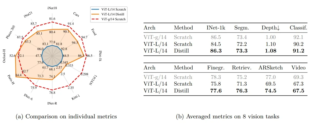
These results confirm that the inductive biases and feature geometry learned by a larger DINOv2 model can be successfully transferred to a smaller student. In practice, this provides an efficient path to deployable self-supervised models that maintain high accuracy while reducing inference cost and memory requirements.
Transfer to Diverse Visual Tasks Beyond classification, DINOv2 exhibits strong generalization across a range of dense prediction and metric-based tasks—despite being trained without labels and without task-specific adaptations.
Semantic and Instance Segmentation. DINOv2 achieves competitive performance on benchmarks such as ADE20K and COCO. When using frozen features followed by linear or shallow heads, ViT-B/14 and ViT-L/14 backbones match or exceed methods like MAE and iBOT on both segmentation accuracy (mIoU) and detection precision (AP). These results validate the spatial expressivity of DINOv2 features, enabled by its patch-level self-distillation.
Depth Estimation. When evaluated on indoor datasets such as NYUv2, DINOv2 features yield accurate monocular depth predictions using only linear regression from frozen embeddings. This suggests that the model encodes strong geometric priors and scene structure, despite never being trained on 3D data.
Image Retrieval. Without task-specific finetuning, DINOv2 achieves state-of-the-art zero-shot retrieval results across multiple datasets. Its features exhibit high instance-level precision under cosine or Euclidean similarity, demonstrating robustness to intra-class variation and viewpoint shifts.
Fine-Grained Classification. On datasets such as Oxford Pets and CUB-200, DINOv2 achieves strong accuracy using frozen backbones with linear classifiers. These results indicate that the model captures detailed attribute-level signals relevant for fine-grained recognition.
Summary. These results underscore DINOv2’s versatility: a single frozen backbone trained on unlabeled images yields linearly decodable features spanning global semantics and local spatial cues. Yet, as models and datasets continue to scale, new challenges emerge—most notably the degradation of dense patch-level features and the need for resolution robustness. These limitations motivate DINOv3, which extends DINOv2 with stability-oriented innovations such as Gram anchoring, high-resolution adaptation, and efficient multi-student distillation, while preserving strong global transferability.
22.4.7 DINOv3: Quick Overview
Motivation DINOv2 22.4.6 introduced a strong self-distillation recipe: ViTs trained on unlabeled images can be used as frozen backbones whose features are linearly decodable for both global and local tasks. When researchers attempted to scale this recipe—training new models from scratch with larger ViTs, broader curated corpora, and longer teacher–student schedules—three limits consistently surfaced and constrained dense transfer in practice:
- Dense feature degradation. In extended self-distillation runs, the global (CLS) embedding continues to improve for image-level classification, but patch-level tokens gradually lose semantic organization. Inter-patch similarities and attention align less reliably with real object boundaries or parts. As a result, a backbone that excels at classification provides weaker frozen features for segmentation, detection, or correspondence. This drift originates in the training dynamics and directly reduces the backbone’s utility for dense tasks.
- Resolution sensitivity. Models trained predominantly at a fixed resolution (e.g., \(224\)) with standard resize–crop internalize a positional geometry and token layout tuned to that scale. When the same backbone is applied to larger images (\(384\)–\(768\) px) or unusual aspect ratios, spatial calibration slips and local consistency degrades. Global probes remain strong, but dense predictions suffer.
- Training efficiency. Producing a full family of deployable backbones by training each student independently is compute-heavy. Long schedules further intensify feature drift and resolution brittleness. A recipe that can produce multiple high-quality backbones in one pass, while preserving dense semantics and improving resolution transfer, is critical for making frozen towers broadly reusable.
DINOv3 is motivated by addressing these shortcomings: stabilizing patch-level semantics during long training, ensuring that frozen encoders generalize across resolutions and aspect ratios, and amortizing pretraining costs while delivering a versatile suite of vision backbones.
What DINOv3 changes DINOv3 updates the DINOv2 recipe with targeted mechanisms that tackle these limits while retaining the simplicity of teacher–student self-distillation.
- Relational stabilization. A Gram anchoring loss matches student and teacher pairwise relations among patch embeddings by aligning their Gram matrices. This preserves neighborhood structure and inter-patch similarities, counteracting late-stage drift and keeping object- and part-level cues coherent in the frozen dense features.
- Resolution robustness. A short high-resolution adaptation phase with positional-encoding jitter re-calibrates token geometry for larger inputs and varied aspect ratios. The same frozen backbone then maintains spatial alignment at higher resolutions common in detection and segmentation without sacrificing global recognition.
- Efficient multi-student distillation. One strong teacher supervises multiple students of different capacities in parallel, sharing the expensive teacher forward pass. This amortizes compute and produces a family of backbones—from lightweight to very large—with consistent feature quality for different latency and memory budgets.
- Expanded, curated data regime. Beyond raw scale, stronger curation and balance broaden concept coverage and stabilize patch-level statistics. This improves both global transfer and the spatial consistency demanded by dense tasks across diverse domains.
Position in the SSL landscape Building on MoCo, BYOL, and DINOv2 [220, 194, 71, 477], DINOv3 pushes three fronts. Dense patch-level learning. Unlike purely global embedding approaches, it supervises and stabilizes per-token structure, enabling strong dense prediction with lightweight heads. Scalability. Larger ViTs trained on vastly larger, better-curated corpora remain stable, yielding robust features across domains. Universality. Frozen representations are competitive with supervised baselines on classification, segmentation, detection, depth, and retrieval, reducing reliance on labeled data.
DINOv3 is a scaled, universal vision backbone that stabilizes what matters for dense transfer. By preserving inter-patch structure, re-aligning for higher resolutions, distilling many students efficiently, and training on a broader curated corpus, it retains DINOv2’s global strengths while delivering substantially more reliable local features. The next part quantifies these effects relative to 22.4.6 and ablates the contribution of each component.
Practical gains For practitioners, DINOv3 provides a stronger and more universal foundation than earlier self-supervised backbones. It is trained at unprecedented scale—up to 7B-parameter ViTs on 1.7B carefully curated images—where the curation pipeline filters out duplicates and low-quality samples while balancing semantic coverage. This results in frozen encoders with both robust global features and stable dense representations. Compared to 22.4.6, DINOv3 improves linear probing on ImageNet by several points, narrows the gap with fully supervised baselines, and yields consistent gains on dense tasks, e.g., +2.4 mIoU on ADE20K semantic segmentation and +1.8 mAP on COCO detection. These improvements transfer smoothly across resolutions and domains, making the features more reliable for real-world inputs. In addition, a family of distilled variants is released, offering models from lightweight to billion-scale with aligned feature geometry. In practice, DINOv3 is not just bigger—it is more curated, more stable, and more versatile, giving practitioners a dependable starting point for classification, detection, segmentation, retrieval, or depth estimation pipelines.
From Self-Distillation to Clustering-Based Objectives
The self-supervised methods explored thus far—including BYOL, SimSiam, DINO, iBOT, DINOv2 and DINOv3, all belong to the family of self-distillation approaches. These frameworks rely on predictive objectives: the model learns to align the representations of differently augmented views of the same image, often using momentum encoders, stop-gradient mechanisms, depending mostly on asymmetries to progress learning. Whether operating at the level of global features (e.g., CLS tokens) or local patch embeddings, these methods implicitly structure the representation space by enforcing consistency across views.
Prediction is not the only route to self-supervision. A distinct line of research instead uses clustering-based objectives, which partition the feature space into discrete prototype assignments so that similar images group together. To avoid collapse onto a few prototypes, these methods enforce constraints such as entropy regularization or balanced assignments. A central example is SwAV (Swapped Assignments between Views), which performs online prototype assignment for each view and enforces cross-view consistency by swapping assignments. Balanced prototype usage is ensured through Sinkhorn–Knopp centering, a mechanism later echoed in DINOv2. SwAV thus bridges contrastive learning and unsupervised clustering, providing an alternative path toward semantically structured representations.
22.5 Clustering Methods
22.5.1 SwAV: Online Clustering via Swapped Assignments
From Contrastive Bottlenecks to Clustering-Based Self-Supervision In the early evolution of self-supervised learning, contrastive methods such as SimCLR and MoCo achieved strong performance by optimizing for instance-level discrimination. These methods learn features by attracting embeddings from augmented views of the same image while repelling embeddings of different images, typically using a contrastive loss such as InfoNCE. However, this approach incurs a computational bottleneck: it requires either extremely large batch sizes (e.g., 4096+ in SimCLR) or auxiliary structures such as memory queues (as in MoCo) to sample sufficient negatives.
SwAV (Swapping Assignments between Views) [72] proposes a fundamentally different formulation. Instead of comparing embeddings pairwise, SwAV performs online clustering by assigning features to a set of learned prototypes and enforcing consistency of these assignments across different augmentations of the same image. This eliminates the need for negatives while retaining the alignment pressure of contrastive learning. Crucially, the model is trained to predict the cluster assignment of one view using the features from another—a formulation known as swapped prediction.
SwAV thus reinterprets contrastive learning as a form of clustering consistency, where the supervision signal is not continuous similarity but rather discrete soft assignments. Features are grouped online using the Sinkhorn-Knopp algorithm, which computes entropy-regularized transport plans to ensure balanced and diverse assignments.
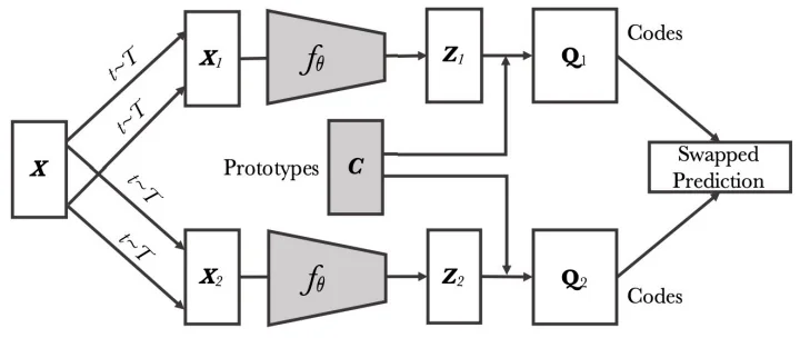
Key Innovations in SwAV:
- Online clustering with balanced assignments: Instead of relying on offline k-means, SwAV performs batch-wise clustering during training by computing soft prototype assignments via Sinkhorn–Knopp. This ensures that all prototypes are equally used and prevents collapse.
- Swapped prediction loss: The model predicts the cluster assignment of one view using features from another, promoting cross-view consistency at the prototype level.
- Multi-crop augmentation: SwAV introduces multiple resolutions of image crops (e.g., 2 global + 6 local), increasing data diversity and boosting learning efficiency without enlarging the batch size.
In the following parts, we describe SwAV’s architectural design, its clustering-based objective, the Sinkhorn-Knopp assignment procedure, and its empirical advantages over the traditional contrastive methods.
Architecture and Training Pipeline
SwAV introduces a clustering-based approach to self-supervised learning that forgoes instance-level comparisons and negative pairs. Instead, it learns semantically meaningful representations by predicting the cluster assignment (or code) of one view from the embedding of another—a strategy known as swapped prediction. This framework builds on a standard encoder–projector backbone and is driven by three key components: multi-crop augmentation, online clustering using learnable prototypes, and balanced code assignment via entropy-regularized optimal transport.
Multi-crop Augmentation and Swapped Prediction Each training image is augmented into multiple crops of varying scale:
- Two global views \(x_{s_1}, x_{s_2} \in \mathbb {R}^{224 \times 224}\), capturing full-scene semantics;
- Several local views \(x_{t_1}, x_{t_2}, \dots \in \mathbb {R}^{96 \times 96}\), capturing fine-grained details.
All views are processed by a shared encoder \(f_\theta \), typically a ResNet-50 or ResNet-200, followed by a two-layer MLP projector \(g_\phi \). This yields embeddings \(z \in \mathbb {R}^D\), with \(D = 128\), that are normalized to lie on the unit hypersphere: \[ z = \frac {g_\phi (f_\theta (x))}{\|g_\phi (f_\theta (x))\|_2} \] Each embedding computes a softmax prediction \(p \in \Delta ^K\) over a set of shared learnable prototypes \(C = [c_1, \dots , c_K] \in \mathbb {R}^{K \times D}\): \[ p^{(k)} = \frac {\exp (z^\top c_k / \tau )}{\sum _{k'=1}^K \exp (z^\top c_{k'} / \tau )}, \] where \(\tau \) is a temperature parameter. These predictions are produced by all crops—both global and local.
Code generation via balanced Sinkhorn assignment. As in DINOv2’s centering mechanism (see Enrichment 22.4.6), SwAV uses the Sinkhorn–Knopp algorithm to convert unnormalized dot-product scores between embeddings and prototypes into a balanced assignment matrix. Specifically, only the two global views per image contribute target codes. Let \( Z \in \mathbb {R}^{D \times B} \) denote the matrix of \( B \) global view embeddings and \( C \in \mathbb {R}^{K \times D} \) the prototype matrix. The dot products \( S = C Z \in \mathbb {R}^{K \times B} \) serve as unnormalized affinity scores between views and prototypes.
These scores are first sharpened and exponentiated to form a nonnegative affinity matrix: \[ A_{ij} = \exp \left ( \frac {[C Z]_{ij}}{\tau } \right ), \quad \mbox{for } 1 \leq i \leq K,\, 1 \leq j \leq B. \]
Unlike softmax, this operation does not normalize rows or columns; instead, SwAV applies Sinkhorn–Knopp to produce a balanced assignment \( Q \in \mathbb {R}^{K \times B} \) of the form: \[ Q = \operatorname {diag}(u)\, A\, \operatorname {diag}(v), \] where \( u \in \mathbb {R}_{>0}^K \) and \( v \in \mathbb {R}_{>0}^B \) are scaling vectors computed iteratively. After just a few iterations (typically 3–5), this procedure yields a matrix that satisfies the marginal constraints: \[ Q \mathbf {1}_B = \tfrac {1}{K} \mathbf {1}_K, \qquad Q^\top \mathbf {1}_K = \tfrac {1}{B} \mathbf {1}_B. \]
These constraints guarantee:
- Each prototype is used equally across the batch.
- Each sample receives a valid probability distribution over the \(K\) prototypes.
The columns of \( Q \) thus define the target codes \( q_s \in \Delta ^K \) for each global view, which are treated as fixed during training and used in the swapped prediction loss.
This balanced assignment strategy—identical in spirit to DINOv2’s centering approach—prevents collapse by enforcing uniform prototype utilization and ensures diverse, high-entropy targets throughout training. Because the prototype matrix \( C \) is trained jointly with the encoder, SwAV learns to maintain semantically meaningful clusters in a fully online and differentiable fashion.
Training Objective and Prototype Updates SwAV’s core learning signal is derived from the swapped prediction loss: each view \(z_t\) (whether global or local) is trained to match the target code \(q_s\) of a different global view from the same image: \[ \ell (z_t, q_s) = - \sum _{k=1}^K q_s^{(k)} \log p_t^{(k)}. \] Each global crop predicts the other’s code, and local crops are split between them. The loss is symmetrized and averaged across all eligible view–target pairs in the batch.
Because the codes \(q_s\) are treated as fixed labels (no gradient flows into them), the model is forced to adjust both its encoder and prototypes to improve predictive accuracy. In particular, the gradient signal updates the prototype matrix \(C\), which is implemented as a linear layer without bias or activation. This allows the cluster centers to adapt continuously to the evolving embedding space.
Stability and scalability. Two design decisions prevent degenerate solutions:
- The balanced assignment constraint ensures that all prototypes are used uniformly within each batch.
- A stop-gradient on the targets \(q_s\) prevents prototypes from simply drifting to match predictions.
Additionally, the prototype weights are frozen for the first epoch to give embeddings time to spread out before clustering begins. The Sinkhorn step is applied only to global crops, so adding more local views increases gradient signal at negligible additional cost.
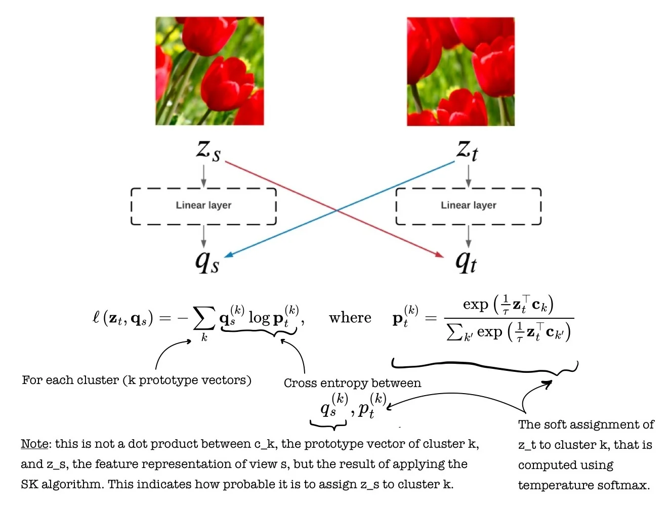
Summary SwAV’s architecture learns representations using:
- Soft prediction: Every crop \(x\) yields an embedding \(z\) that predicts a probability distribution \(p\) over the prototype set \(C\) via dot-product similarity.
- Balanced code generation: Global crops generate target codes \(q_s\) through Sinkhorn-based optimal transport, enforcing uniform use of prototypes.
- Swapped prediction loss: The model is trained to align the prediction \(p_t\) of one view to the code \(q_s\) of another, encouraging semantic consistency across views.
This design eliminates the need for negatives, momentum encoders, or memory banks, while achieving efficient, scalable, and semantically meaningful feature learning with a standard CNN backbone.
Empirical Results and Key Findings
SwAV introduced a new paradigm for self-supervised learning by coupling multi-crop augmentation with online clustering and swapped prediction. This design proved empirically successful across both standard linear evaluation and a wide range of downstream transfer tasks, offering strong performance while remaining efficient and scalable.
Benchmarking on ImageNet SwAV was the first self-supervised method to exceed 75% top-1 accuracy on ImageNet using a standard ResNet-50 under the linear evaluation protocol. With 75.3% accuracy after 800 epochs [72], it significantly outperformed earlier approaches such as SimCLR (69.3%), MoCo v2 (71.1%), and BYOL (74.3%). This result brought SwAV within 1.2% of supervised pretraining (76.5%)—a major milestone at the time. Scaling to a ResNet-50-w5 architecture pushes accuracy even further, reaching 78.5%.
Transfer to Downstream Tasks SwAV also excels on transfer benchmarks. On VOC07+12 detection (AP50), it surpasses supervised training by over 1 point (82.6 vs. 81.3). On COCO, it improves over the supervised baseline in both object detection (41.6 vs. 39.7 AP) and instance segmentation (37.8 vs. 35.9 mask AP). These results show that SwAV’s representations generalize better across tasks, benefiting from their semantic grounding and scale invariance.
Training Efficiency and Accessibility A defining strength of SwAV is its performance under constrained settings. While SimCLR required extremely large batch sizes (e.g., 4096), SwAV achieves competitive accuracy (74.3%) with a batch size of just 256 and training for 400 epochs. This efficiency stems from its design: SwAV avoids the need for memory banks, negative pairs, or momentum encoders, relying instead on multi-view prediction with a small set of balanced targets.
Ablation Highlights SwAV’s design was supported by extensive ablation studies [72], which revealed the distinct contribution of each architectural component:
- Multi-crop augmentation was the most impactful addition. When training a ResNet-50 for 200 epochs on ImageNet without a feature queue, adding 6 low-resolution local crops (\(96 \times 96\)) to the standard 2 global crops (\(224 \times 224\)) improved linear accuracy from 66.2% to 70.7%—a gain of \(+4.5\%\). This strategy multiplies training signal without significantly increasing compute or memory, and was later adopted by DINO and iBOT.
- Prototype count showed strong robustness. Varying the number of prototypes from \(K = 3{,}000\) to \(K = 15{,}000\) had negligible impact on final accuracy (\(\leq 0.3\%\)), provided Sinkhorn balancing was applied. The method remained effective as long as the prototype set was sufficiently overcomplete relative to batch size.
- Sinkhorn–Knopp assignment proved essential: replacing Sinkhorn with unbalanced softmax assignments caused significant degradation—dropping top-1 accuracy by over \(3\%\)—highlighting the importance of balanced code usage to avoid prototype collapse.
Impact and Legacy SwAV demonstrated that online clustering with learnable prototypes, when combined with scale-diverse views and efficient balancing, could rival and even surpass contrastive learning. Its innovations reduced computational overhead, improved convergence, and enabled strong transfer performance—all within a streamlined ResNet-based pipeline. These ideas laid critical groundwork for the next generation of self-supervised methods, including DINO and iBOT, and remain influential in the field.
22.6 Feature Decorrelation Methods
22.6.1 Barlow Twins: Feature Decorrelation without Negatives
Barlow Twins [774] is a simple yet effective self-supervised method that encourages representations to be simultaneously invariant to augmentations and decorrelated across features. It belongs to a broader class of decorrelation-based self-supervised learning approaches that aim to avoid representational collapse without relying on contrastive loss, negative pairs, or momentum encoders.
The method is named after neuroscientist Horace Barlow, whose redundancy reduction hypothesis posits that sensory systems learn to represent stimuli in a compact, non-redundant way. In this spirit, Barlow Twins learns representations that capture unique, non-overlapping information in each dimension—maximizing utility for downstream tasks.
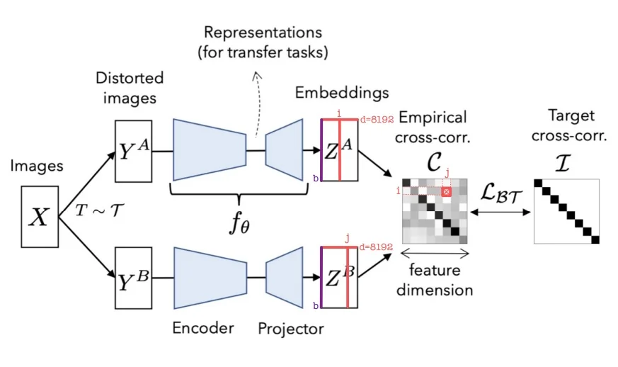
Method Overview Barlow Twins formulates representation learning as a redundancy-reduction problem guided by self-supervised invariance. Given a training image \( \mathbf {X} \in \mathbb {R}^{H \times W \times 3} \), two independent stochastic augmentations \( \tau ^A, \tau ^B \sim \mathcal {T} \) produce views: \[ \mathbf {Y}^A = \tau ^A(\mathbf {X}), \qquad \mathbf {Y}^B = \tau ^B(\mathbf {X}). \] These are processed by a shared encoder–projector stack \( g_\phi \circ f_\theta \), yielding normalized embeddings: \[ \mathbf {z}^A = \frac {g_\phi (f_\theta (\mathbf {Y}^A))}{\|g_\phi (f_\theta (\mathbf {Y}^A))\|_2}, \qquad \mathbf {z}^B = \frac {g_\phi (f_\theta (\mathbf {Y}^B))}{\|g_\phi (f_\theta (\mathbf {Y}^B))\|_2} \]
Over a mini-batch of size \( B \), we stack the normalized embeddings into matrices \( \mathbf {Z}^A, \mathbf {Z}^B \in \mathbb {R}^{B \times D} \). The core statistic in Barlow Twins is the empirical cross-correlation matrix \( \mathbf {C} \in \mathbb {R}^{D \times D} \), defined as: \[ \mathbf {C} = \frac {1}{B} (\mathbf {Z}^A)^\top \mathbf {Z}^B, \qquad C_{ij} = \frac {1}{B} \sum _{b=1}^B z^{A(i)}_b \, z^{B(j)}_b. \] Each entry \( C_{ij} \) measures the linear correlation between the \( i \)-th feature in view A and the \( j \)-th feature in view B, with values in the range \( [-1, 1] \). Intuitively:
- \( C_{ij} = 1 \): perfect positive correlation—features vary identically across the batch.
- \( C_{ij} = 0 \): statistical independence—no linear correlation.
- \( C_{ij} = -1 \): perfect negative correlation—still redundant and thus undesirable.
Barlow Twins aims to make \( \mathbf {C} \approx \mathbf {I}_D \), the identity matrix, based on two key principles:
- (i)
- Invariance: pushing each diagonal entry \( C_{ii} \to 1 \) ensures that each feature remains stable across augmented views of the same image;
- (ii)
- Redundancy reduction: minimizing off-diagonal entries \( C_{ij} \to 0 \) for \( i \ne j \) encourages features to be decorrelated and non-redundant.
This objective encourages the learned representation to be both semantically consistent and informationally diverse—qualities essential for downstream generalization.
Redundancy Reduction Loss The training loss penalizes any deviation of \( \mathbf {C} \) from the identity: \[ \mathcal {L}_{\mbox{BT}} \; \triangleq \; \underbrace {\sum _{i=1}^D (1 - C_{ii})^2}_{\mbox{\small invariance term}} \;+\; \lambda \underbrace {\sum _{i=1}^D \sum _{j \ne i} C_{ij}^2}_{\mbox{\small redundancy reduction term}}. \tag {BT} \] Here, \( \lambda \) is a weighting coefficient that balances the importance of diagonal preservation and off-diagonal suppression. The original paper sets \( \lambda = 5 \times 10^{-3} \) and reports robustness to this choice [774].
Intuition. The first term ensures that each embedding dimension captures consistent semantic content across augmented views (invariance), while the second term discourages redundancy by pushing feature dimensions to be statistically independent.
- The loss is computed on the batchwise cross-correlation, avoiding the need for negative pairs, momentum encoders, or memory banks.
- Gradients propagate through all features and samples due to the fully differentiable nature of \( \mathbf {C} \).
- Prior to computing \( \mathbf {C} \), the embedding vectors are batch-normalized to have zero mean and unit variance—without affine parameters—to stabilize statistics.
In contrast to contrastive or distillation-based frameworks, Barlow Twins achieves both invariance and feature diversity in a fully symmetric manner, using only positive pairs from the same image. Its loss structure alone is sufficient to prevent representational collapse.
Empirical Results and Ablation Studies
Barlow Twins delivers strong empirical performance across both standard self-supervised benchmarks and downstream transfer tasks. Despite its architectural simplicity and the absence of negative pairs, teacher networks, or asymmetric encoders, the method achieves competitive results through a symmetric objective that jointly enforces invariance and redundancy reduction.
Linear Evaluation on ImageNet In the standard linear probing setup on ImageNet-1K, Barlow Twins achieves 73.2% top-1 and 91.0% top-5 accuracy using a ResNet-50 trained for 1000 epochs [774]. This outperforms earlier contrastive baselines such as SimCLR (69.3%) and MoCo v2 (71.1%), and comes close to SwAV (75.3%) and BYOL (74.3%), despite using neither multi-crop augmentation nor a momentum encoder.
| Method | Top-1 (%) | Top-5 (%) |
|---|---|---|
| Supervised | 76.5 | – |
| MoCo | 60.6 | – |
| PIRL | 63.6 | – |
| SimCLR | 69.3 | 89.0 |
| MoCo v2 | 71.1 | 90.1 |
| SimSiam | 71.3 | – |
| SwAV (no multi-crop) | 71.8 | – |
| BYOL | 74.3 | 91.6 |
| SwAV | 75.3 | – |
| Barlow Twins | 73.2 | 91.0 |
Transfer Learning Performance Barlow Twins generalizes well to diverse downstream tasks. When frozen ResNet-50 features are evaluated via linear classifiers, the model performs comparably to SwAV and BYOL and consistently outperforms/on par with SimCLR and MoCo v2. These results—summarized in the following table—highlight the semantic richness and generality of the representations learned through the Barlow Twins objective.
| Method | Places-205 | VOC07 (mAP) | iNat18 |
|---|---|---|---|
| Supervised | 53.2 | 87.5 | 46.7 |
| SimCLR | 52.5 | 85.5 | 37.2 |
| MoCo v2 | 51.8 | 86.4 | 38.6 |
| SwAV (no multi-crop) | 52.8 | 86.4 | 39.5 |
| SwAV | 56.7 | 88.9 | 48.6 |
| BYOL | 54.0 | 86.6 | 47.6 |
| Barlow Twins | 54.1 | 86.2 | 46.5 |
Ablation Studies Controlled ablations confirm that both terms of the loss—the invariance and redundancy penalties—are essential. The following table shows that removing either term severely degrades performance. Notably, using only the redundancy term causes collapse. Additional findings include:
- Normalization matters: Applying feature-wise normalization before computing the cross-correlation matrix improves stability.
- BatchNorm in the MLP improves performance, though the method is fairly robust without it.
- Loss formulation is key: Replacing the objective with a temperature-scaled softmax cross-entropy reduces top-1 accuracy by more than 8%.
| Configuration | Top-1 (%) | Top-5 (%) |
|---|---|---|
| Full loss (default) | 71.4 | 90.2 |
| Only invariance term | 57.3 | 80.5 |
| Only redundancy term | 0.1 | 0.5 |
| Feature-wise normalization | 69.8 | 88.8 |
| No BN in MLP | 71.2 | 89.7 |
| No BN + No normalization | 53.4 | 76.7 |
| Cross-entropy w/ temperature | 63.3 | 85.7 |
Batch Size Robustness Barlow Twins performs well even at small batch sizes. The following figure shows that, unlike SimCLR and BYOL, it maintains high accuracy at batch sizes as low as 256. This is because it does not rely on in-batch negatives or queue-based comparisons.
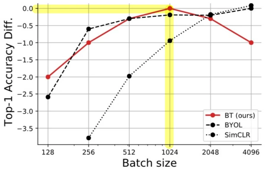
Effect of Projector Dimensionality The following figure illustrates how Barlow Twins benefits from larger embedding dimensions. Unlike SimCLR and BYOL, which plateau or degrade with wider projections, Barlow Twins continues to improve up to 8192 or even 16384 dimensions—likely due to its decorrelation objective.
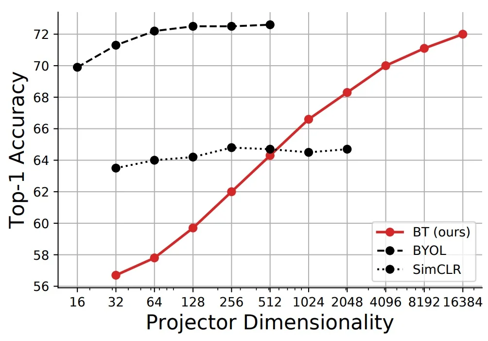
Sensitivity to Augmentations The following figure shows how performance declines as augmentations are progressively weakened. Barlow Twins is more robust than SimCLR, but slightly less stable than BYOL, whose architectural asymmetry offers stronger inductive bias under weak views.
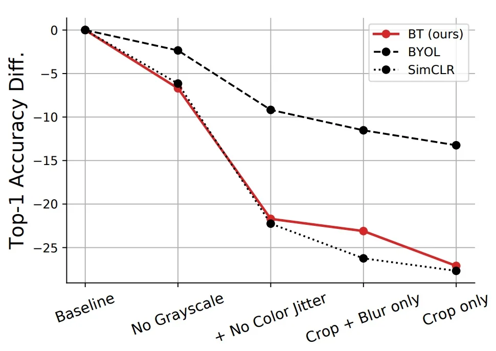
Hyperparameter Stability The loss function in Barlow Twins consists of two complementary terms: one that enforces invariance across augmented views by driving the diagonal of the cross-correlation matrix \( \mathbf {C} \) toward 1, and another that encourages decorrelation by penalizing off-diagonal terms. The scalar hyperparameter \( \lambda \) controls the relative importance of the redundancy reduction objective: \[ \mathcal {L}_{\mbox{BT}} = \sum _i (1 - C_{ii})^2 + \lambda \sum _{i} \sum _{j \ne i} C_{ij}^2. \] While in principle tuning \( \lambda \) could affect convergence and representation quality, Barlow Twins exhibits remarkable robustness to its value. As shown in the following figure, top-1 accuracy remains stable across several orders of magnitude of \( \lambda \), simplifying deployment and hyperparameter tuning.
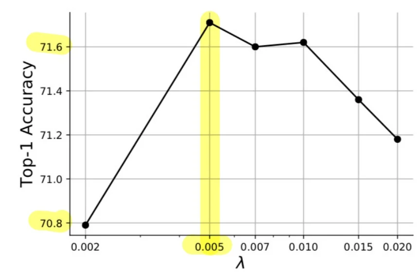
Summary and Outlook Barlow Twins achieves state-of-the-art performance with a remarkably simple and symmetric training objective. By maximizing invariance while minimizing redundancy, it learns representations that are both stable across views and statistically diverse—without relying on negative pairs, momentum encoders, or asymmetric architectures. These principles underpin a broader family of non-contrastive methods that favor structured, constraint-based losses over explicit comparison.
In the next part, we examine VicReg (Variance-Invariance-Covariance Regularization), which builds on these ideas by decomposing the objective even further. Unlike Barlow Twins, VicReg drops the cross-correlation matrix in favor of three explicit terms—each corresponding to a statistical property of the learned features—and enables even greater control over the representation geometry.
22.6.2 VICReg: Variance-Invariance-Covariance Regularization
VICReg [27] introduces a simple yet powerful objective for self-supervised learning that avoids collapse using only positive pairs. The learning signal is decomposed into three distinct components:
- Invariance loss \( \mathcal {L}_{\mbox{sim}} \): aligns the embeddings of different augmentations of the same image to ensure consistent representation.
- Variance loss \( \mathcal {L}_{\mbox{var}} \): maintains a minimum standard deviation across each embedding dimension to prevent representational collapse.
- Covariance loss \( \mathcal {L}_{\mbox{cov}} \): penalizes redundancy by minimizing off-diagonal entries of the covariance matrix across embedding dimensions.
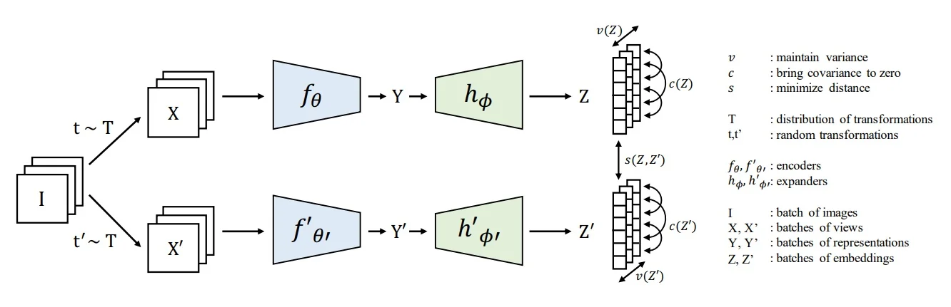
The architecture follows a symmetric dual-branch design (Figure 22.64). A batch of images \( I \) is augmented twice using transformations \( t, t' \sim \mathcal {T} \) to produce two views: \[ X = t(I), \qquad X' = t'(I). \] These views are encoded by two networks \( f_\theta \) and \( f'_{\theta '} \) (typically sharing weights) to produce intermediate features: \[ Y = f_\theta (X), \qquad Y' = f'_{\theta '}(X'). \] A projection MLP, called an expander, maps these features to final embeddings: \[ Z = h_\phi (Y), \qquad Z' = h'_{\phi '}(Y') \in \mathbb {R}^{B \times D}, \] where \( B \) is the batch size and \( D \) is the embedding dimensionality.
We summarize VICReg’s notation and architecture:
- \( \mathcal {T} \): Stochastic data augmentation distribution.
- \( t, t' \sim \mathcal {T} \): Two sampled augmentations.
- \( I \): Input batch of images.
- \( X = t(I),\; X' = t'(I) \): Augmented views of the input.
- \( f_\theta , f'_{\theta '} \): Encoders (typically ResNet-50).
- \( h_\phi , h'_{\phi '} \): Expander MLPs (usually 3-layer).
- \( Y = f_\theta (X),\; Y' = f'_{\theta '}(X') \): Intermediate feature vectors.
- \( Z = h_\phi (Y),\; Z' = h'_{\phi '}(Y') \in \mathbb {R}^{B \times D} \): Final embeddings used in the VICReg loss.
The overall objective is a weighted sum of three losses: \[ \mathcal {L}_{\mbox{VICReg}}(Z, Z') = \lambda _s\, \mathcal {L}_{\mbox{sim}}(Z, Z') + \lambda _v\, \mathcal {L}_{\mbox{var}}(Z, Z') + \lambda _c\, \mathcal {L}_{\mbox{cov}}(Z, Z'), \] where:
- \( \mathcal {L}_{\mbox{sim}} \) ensures invariance by pulling corresponding embeddings \( Z \) and \( Z' \) together,
- \( \mathcal {L}_{\mbox{var}} \) maintains per-dimension variance across the batch, enforcing feature spread and avoiding collapse,
- \( \mathcal {L}_{\mbox{cov}} \) minimizes covariance between different embedding dimensions, encouraging decorrelation.
Default weights are \( \lambda _s = 25.0 \), \( \lambda _v = 25.0 \), and \( \lambda _c = 1.0 \), balancing similarity and statistical regularization for stable training.
In the next parts, we analyze each of these terms in detail—beginning with the invariance loss \( \mathcal {L}_{\mbox{sim}} \)—and explain how their combination avoids representational collapse while encouraging semantically meaningful and diverse feature learning.
Invariance Term: Similarity Loss
The first component of VICReg’s objective promotes invariance to data augmentation. This term encourages embeddings of two augmented views of the same image to be close in Euclidean space, thereby ensuring semantic consistency across different appearances of the same input.
Let a batch of \( B \) input images be augmented twice to produce views \( X \) and \( X' \), which are then mapped to embeddings \( Z, Z' \in \mathbb {R}^{B \times D} \) by the encoder–projector stack. Each row pair \( (z_i, z'_i) \) corresponds to two views of the same image.
The similarity loss is defined as the mean squared error (MSE) between corresponding embeddings: \[ \mathcal {L}_{\mbox{sim}}(Z, Z') = \frac {1}{B} \sum _{i=1}^B \| z_i - z'_i \|_2^2. \] This can be compactly expressed as the squared Frobenius norm: \[ \mathcal {L}_{\mbox{sim}}(Z, Z') = \frac {1}{B} \| Z - Z' \|_F^2. \] This term pulls positive pairs together in the embedding space and plays the same conceptual role as contrastive positives—but without relying on any form of negative sampling.
Why regularization is necessary. While the similarity loss encourages embeddings of augmented views to align, minimizing it alone is insufficient—it admits a trivial solution where all embeddings collapse to a constant vector (e.g., \( z_i = z'_i = \mathbf {0} \)). Such a degenerate outcome minimizes the loss but eliminates all useful information.
Unlike prior methods such as BYOL or SimSiam, which prevent collapse through architectural asymmetry (e.g., predictor networks, stop-gradient operations, or momentum encoders), VICReg avoids these design complexities. Instead, it tackles collapse directly and explicitly by introducing two additional regularizers: a variance term that enforces feature spread across the batch, and a covariance term that reduces feature redundancy.
In the following parts, we present the variance and covariance regularizers that ensure each embedding dimension maintains spread across the batch and captures decorrelated information. Together with the similarity term, these components allow VICReg to learn rich, invariant features without relying on negatives or specialized architectural tricks.
Variance Term: Spread Preservation
The second component of VICReg’s loss prevents dimensional collapse by enforcing variability across samples in each embedding dimension. This is achieved by penalizing dimensions whose batchwise standard deviation falls below a fixed threshold.
Let \( Z, Z' \in \mathbb {R}^{B \times D} \) denote the two batches of embeddings. For each feature dimension \( j \in \{1, \dots , D\} \), define \( Z_{\cdot j} \in \mathbb {R}^B \) as the \( j \)-th column of \( Z \), representing the values of feature \( j \) across the batch. The variance loss on \( Z \) is defined as: \[ \mathcal {L}_{\mbox{var}}(Z) = \frac {1}{D} \sum _{j=1}^D \max \left ( 0, \gamma - \sqrt {\operatorname {Var}(Z_{\cdot j}) + \epsilon } \right ), \] where \( \gamma > 0 \) is a target standard deviation (typically \( \gamma = 1 \)), and \( \epsilon \) is a small constant (e.g., \( 10^{-4} \)) for numerical stability.
This ReLU-style hinge penalty activates only when the standard deviation of a feature falls below \( \gamma \), ensuring that each embedding dimension retains sufficient variation across the batch.
The full variance loss is applied symmetrically to both embedding branches: \[ \mathcal {L}_{\mbox{var}}(Z, Z') = \mathcal {L}_{\mbox{var}}(Z) + \mathcal {L}_{\mbox{var}}(Z'). \]
Intuition. Without this term, the model could minimize the similarity loss by collapsing all features to a constant vector (e.g., \( Z = Z' = \mathbf {0} \)), which yields zero variance and no discriminative power. The variance constraint ensures that each dimension remains active and informative by enforcing a lower bound on its spread. Unlike whitening, which imposes full normalization, VICReg simply avoids collapse by preventing features from becoming degenerate—making the constraint both flexible and effective.
Next, we introduce the covariance regularizer, which complements this spread constraint by encouraging statistical independence between different feature dimensions.
Covariance Term: Redundancy Reduction
The third and final component of VICReg’s objective addresses feature redundancy. While the variance loss ensures that each embedding dimension is active across the batch, the covariance loss encourages decorrelation—ensuring that each feature captures distinct information.
Let \( Z \in \mathbb {R}^{B \times D} \) denote a batch of zero-mean embeddings. The empirical covariance matrix of \( Z \) is given by: \[ \Sigma (Z) = \frac {1}{B - 1} Z^\top Z \in \mathbb {R}^{D \times D}, \] where the diagonal elements capture featurewise variance (already handled by \( \mathcal {L}_{\mbox{var}} \)) and the off-diagonal elements encode pairwise linear correlations between feature dimensions.
The covariance loss penalizes these off-diagonal entries: \[ \mathcal {L}_{\mbox{cov}}(Z) = \frac {1}{D} \sum _{i \ne j} \left [ \Sigma (Z) \right ]_{ij}^2 = \frac {1}{D} \sum _{i \ne j} \left ( \frac {1}{B - 1} Z_{\cdot i}^\top Z_{\cdot j} \right )^2, \] where \( Z_{\cdot i} \in \mathbb {R}^{B} \) denotes the \( i \)-th column of \( Z \), and the squared inner products quantify correlation magnitude.
This term is symmetrized across both embedding branches: \[ \mathcal {L}_{\mbox{cov}}(Z, Z') = \mathcal {L}_{\mbox{cov}}(Z) + \mathcal {L}_{\mbox{cov}}(Z'). \]
Intuition. High off-diagonal covariance implies that multiple features are encoding similar information, reducing representational efficiency. The covariance loss explicitly discourages such redundancy by driving these correlations toward zero. This acts as a soft whitening constraint, but without requiring full matrix inversion or decorrelation, and without interfering with the variance term. Unlike methods that implicitly encourage feature decorrelation via batch normalization or orthogonality constraints, VICReg enforces redundancy reduction directly through the loss function in a differentiable and scalable manner.
Loss Summary. Together, the three VICReg losses form a self-contained and collapse-resistant objective:
- \( \mathcal {L}_{\mbox{sim}} \): aligns paired views to promote augmentation invariance.
- \( \mathcal {L}_{\mbox{var}} \): preserves diversity across samples by enforcing per-dimension spread.
- \( \mathcal {L}_{\mbox{cov}} \): eliminates linear redundancy by decorrelating features.
In the following part, we examine VICReg’s training setup and empirical results—including comparisons to contrastive and non-contrastive baselines across linear probing and transfer learning benchmarks.
Implementation Details and Empirical Evaluation
Training Setup VICReg uses a standard ResNet-50 encoder followed by a three-layer MLP expander. Each hidden layer contains 8192 units with Batch Normalization and ReLU activation. The final embeddings \( Z, Z' \in \mathbb {R}^{B \times D} \) are used directly in the loss computation—without \( \ell _2 \)-normalization or whitening. Training is conducted for 1000 epochs using the LARS optimizer with a base learning rate of 0.3, cosine learning rate decay, and batch size of 2048. The data augmentation strategy matches that of SimCLR.
Linear Evaluation on ImageNet The following table reports ImageNet-1K top-1 accuracy under the standard linear evaluation protocol. VICReg matches the performance of Barlow Twins and significantly outperforms SimCLR, all while avoiding negatives, target networks, or asymmetry. While BYOL achieves slightly higher accuracy, it requires an additional predictor head and momentum encoder.
| Method | Backbone | Top-1 (%) |
|---|---|---|
| SimCLR | ResNet-50 | 69.3 |
| Barlow Twins | ResNet-50 | 73.2 |
| BYOL | ResNet-50 | 74.3 |
| VICReg | ResNet-50 | 73.2 |
Transfer Learning Performance VICReg generalizes well across diverse downstream tasks. The following table shows results on Places205, Pascal VOC07, and iNat18 using frozen ResNet-50 features with linear classifiers. VICReg outperforms SimCLR, Barlow Twins, and BYOL across all benchmarks—particularly on fine-grained classification tasks like iNat18.
Robustness to Batch Size A practical strength of VICReg is its ability to maintain stable performance with small batch sizes. Since VICReg does not rely on contrastive sampling, it avoids the sharp degradation seen in methods like SimCLR. According to Section 5.2 of [27], reducing the batch size from 2048 to 256 results in a drop of less than 1% for VICReg, while SimCLR suffers over 6%.
Summary of Empirical Results VICReg combines competitive performance with architectural simplicity and training efficiency. Its design avoids the pitfalls of earlier SSL methods by explicitly decomposing invariance, variance preservation, and redundancy reduction into three stable, interpretable loss terms. The result is a scalable and robust alternative to both contrastive and distillation-based approaches.
We next examine ablation studies that validate each component of the VICReg loss and highlight the necessity of combining similarity, variance, and covariance terms.
Ablation Studies and Objective Decomposition
To isolate the contribution of each term in the VICReg objective, the authors conduct a series of ablation experiments. These studies clarify how each component—the similarity term \( \mathcal {L}_{\mbox{sim}} \), the variance term \( \mathcal {L}_{\mbox{var}} \), and the covariance term \( \mathcal {L}_{\mbox{cov}} \)—contributes to learning stable, non-degenerate representations. While the similarity loss encourages view alignment, it must be paired with regularizers to prevent collapse and encourage feature diversity.
Effect of Removing Loss Terms The following table reports the impact of disabling different loss components. When the variance term is removed, the network collapses to a trivial solution where all embeddings are constant. Removing the similarity term also causes failure: without alignment between views, no meaningful features are learned. Removing the covariance term does not lead to collapse, but results in highly redundant dimensions and reduced accuracy. All three terms are necessary to achieve invariance, diversity, and disentanglement in the learned representation.
| Loss Configuration | \( \lambda _s \) | Collapse | Top-1 Acc. (%) |
|---|---|---|---|
| sim + var + cov (VICReg) | 25 | ✗ | 68.6 |
| sim + var (no cov) | 1 | ✗ | 57.5 |
| sim + cov (no var) | 25 | ✓ | - |
| var + cov (no sim) | 0 | ✓ | - |
| Only sim | 1 | ✓ | - |
Architectural Robustness VICReg is architecturally flexible. It does not require weight sharing or symmetric encoders. Performance remains strong in non-Siamese setups: when the encoders for the two branches are decoupled, accuracy drops only marginally (from 73.2% to 72.8%). Similarly, reducing the expander from three to two layers results in minimal degradation, demonstrating robustness to projection head configuration.
Comparison with Whitening-Based Methods Unlike methods such as Barlow Twins, which impose an identity constraint on the cross-correlation matrix, VICReg decomposes redundancy reduction into two explicit regularizers: a variance term to preserve spread, and a covariance term to enforce decorrelation. This formulation eliminates the need for batch normalization across views and makes the method more stable—especially when training with smaller batch sizes.
Ablation Summary These findings highlight the distinct and complementary roles of VICReg’s three loss terms:
- Invariance (\( \mathcal {L}_{\mbox{sim}} \)): Aligns positive pairs to enforce view consistency.
- Variance (\( \mathcal {L}_{\mbox{var}} \)): Prevents representational collapse by ensuring each dimension is active across the batch.
- Covariance (\( \mathcal {L}_{\mbox{cov}} \)): Encourages disentanglement by reducing linear redundancy between features.
Together, these components yield a stable and interpretable framework for self-supervised learning—one that avoids contrastive negatives, momentum encoders, and stop-gradient tricks while remaining effective and scalable.
22.7 Adapting SSL to Downstream Tasks
Self-supervised learning (SSL) decouples feature learning from task supervision, producing general-purpose encoders that can be adapted to a wide range of downstream objectives—from classification and retrieval to segmentation and detection. However, deploying these representations effectively requires thoughtful alignment between the pretrained model, the target task, and the available adaptation budget. Factors such as task structure, domain similarity, labeled data availability, and hardware constraints all influence which adaptation strategy will yield the best trade-off between performance, robustness, and efficiency. The following parts present a structured pipeline for downstream transfer, beginning with backbone selection (the focus of this section) and continuing through a hierarchy of adaptation strategies—ranging from simple linear probing to full fine-tuning. By matching model flexibility to task demands, practitioners can harness the full potential of SSL.
22.7.1 Aligning Backbone Structure with Task Demands
The architecture and pretraining objective used in self-supervised learning (SSL) directly influence the type of information encoded by the model. Depending on whether the training strategy emphasizes spatial precision or semantic abstraction, different backbones will excel at different downstream tasks. This subsection outlines how the structural properties of SSL models align with the demands of classification, retrieval, segmentation, and other vision problems.
Masked Image Modeling: Prioritizing Spatial Detail Masked image modeling (MIM)—used in methods such as MAE, iBOT, and DINOv2—trains the encoder to reconstruct masked portions of the input image. This objective forces the model to reason about local textures, edges, and fine spatial patterns.
- These localized features are essential for dense prediction tasks such as semantic segmentation, object detection, and monocular depth estimation.
- For example, adding a MIM objective to DINOv2 improves segmentation accuracy by nearly 3% mIoU on ADE20k compared to global-only training [477].
Contrastive and Clustering Methods: Emphasizing Semantic Structure Contrastive learning approaches like SimCLR and MoCo, and clustering-based methods like SwAV, optimize models to group together different augmented views of the same image while pushing apart views of different images. These objectives lead the model to capture high-level concepts such as object shape and category, rather than spatial details.
- Such models are well-suited for global tasks like image classification and retrieval, where the goal is to assign an image to a broad semantic category or to match instances.
- However, their representations are often less suited for pixel-level predictions, as spatial continuity is not explicitly encouraged during training.
Hybrid Approaches: Balancing Spatial and Semantic Information Modern SSL methods like DINOv2 and EVA incorporate both reconstruction-style and global invariance losses, enabling the model to learn features that capture both spatial granularity and semantic abstraction.
- These hybrid models consistently perform well on both global and dense benchmarks, making them suitable defaults when the downstream task mix is unknown or varied.
- DINOv2, for instance, achieves state-of-the-art linear probing accuracy on ImageNet while also outperforming earlier models on semantic segmentation and depth estimation [477].
- For tasks involving pixel-level supervision (e.g., segmentation, detection), select a model trained with a strong MIM component.
- For tasks emphasizing semantic abstraction (e.g., classification, retrieval), contrastive or clustering-based models are efficient and competitive.
- For multi-task pipelines or general-purpose usage, hybrid models such as DINOv2 offer strong performance across the board.
- When interpretability or simplicity is preferred (e.g., in real-time systems), older contrastive models with convolutional backbones may remain useful baselines.
Understanding whether a downstream task depends more on spatial resolution or semantic discrimination is a critical first step in selecting a suitable SSL backbone. Hybrid models provide broad coverage, but targeted choices remain important when task constraints are well-defined.
22.7.2 Data Distribution and Domain Shift Considerations
Despite the scale and diversity of modern pretraining corpora—e.g., LVD-142M for DINOv2 or LAION-2B for CLIP—downstream datasets often exhibit domain shifts that undermine transfer performance. These shifts may include differences in image content (e.g., medical or satellite imagery), resolution, noise, label distribution, or visual style. Understanding and mitigating this mismatch is essential for effective adaptation of self-supervised models.
Diagnosing Domain Shift Before selecting an adaptation strategy—or even a specific pretrained backbone—it is important to assess how well your downstream data align with the pretraining distribution. In some cases, domain knowledge alone can provide strong cues: for example, highly specialized imagery—such as histology slides, X-rays, or thermal satellite captures—is almost certainly out-of-distribution (OOD) relative to natural-image web corpora like LAION or LVD-142M.
However, beyond intuition, several practical diagnostics can help estimate domain alignment and inform next steps. These tools vary depending on the presence of labels and the type of task:
-
For classification tasks with labeled data:
- Zero-shot \(k\)-NN classification: Extract features using the frozen SSL backbone and train a \(k\)-nearest neighbors classifier on the labeled training set. If accuracy is very low, it suggests the feature space does not align well with semantic categories in your domain.
- t-SNE / UMAP visualization: Project features from the frozen encoder into 2D and color by class label. If clusters are poorly separated or entangled, it indicates that representations may not be semantically structured for the task.
-
For detection, segmentation, or unlabeled data:
- Region-based feature clustering: Extract local features (e.g., via sliding windows or ViT tokens) and apply \(k\)-means clustering. If clusters fail to align with meaningful regions (e.g., objects, organs), this suggests that spatial semantics may not be captured.
- Visual probing: Run pretrained detection or segmentation heads (e.g., COCO-trained Mask R-CNN) using frozen features to visually assess qualitative results. While informal, it can reveal if feature maps support spatial reasoning.
Should We Try Multiple Backbones? In practice, testing multiple pretrained backbones is often valuable—even if the final downstream model will only use one. Running the above diagnostics with two or three strong candidates (e.g., DINOv2, ReLICv2) provides insight into how well each model’s feature space aligns with your data. This can guide both:
- Finetuning strategy selection: If one backbone yields strong frozen-feature performance, lightweight adaptation (e.g., PEFT or a small MLP head) may suffice. If all perform poorly, continued pretraining or full fine-tuning may be needed.
- Model selection itself: In domains with unknown or complex statistics, empirical comparison is often more reliable than purely theoretical choices. Trying multiple backbones during early prototyping can uncover unexpected strengths in certain architectures or pretext objectives.
Summary Domain shift is the central challenge in transferring self-supervised representations. Its presence should be diagnosed early, using both domain knowledge and frozen-feature probes. Depending on the task and data availability, this may also motivate testing multiple SSL backbones before committing to a full adaptation pipeline. These diagnostics inform not only which model to use, but also how aggressive the adaptation strategy must be—ranging from linear probing to full fine-tuning or continued self-supervised training.
22.8 Fine-Tuning Self-Supervised Backbones
Once a self-supervised representation approach has been selected, the next challenge is adapting it to a downstream task. This step is rarely trivial: unlike fully supervised pretraining, self-supervised learning (SSL) does not optimize for any specific end task. As such, even the best SSL features may need further adaptation to achieve peak task-specific performance.
This section presents a structured overview of fine-tuning strategies, grounded in three key factors:
- 1.
- Domain similarity: How similar is the downstream data to the model’s pretraining corpus?
- 2.
- Label availability: Are sufficient labeled examples available, or only unlabeled data?
- 3.
- Resource constraints: How much GPU memory, time, and tuning budget are available?
We organize the landscape of adaptation strategies along a spectrum of increasing capacity and computational cost. Each method offers a different trade-off between preserving pretrained features and adapting to the task at hand.
22.8.1 Choosing an Adaptation Strategy: Data, Domain, and Cost
(1) Linear Probing and Lightweight Heads
The simplest option is to freeze the encoder and train a linear classifier or shallow MLP head on top. This strategy serves two purposes: as a diagnostic tool to evaluate representation quality, and as a minimal adaptation when data or compute is limited.
- Cost: Minimal. Only the top layer/shallow head is trained.
- When to use: Data is scarce, domain shift is low, or task setup favors interpretability and stability.
(2) Parameter-Efficient Fine-Tuning (PEFT)
Parameter-efficient fine-tuning (PEFT) methods adapt large pretrained models by updating only a small subset of parameters—typically fewer than 1–5%—while keeping the main backbone frozen. This significantly reduces GPU memory usage, training time, and the risk of overfitting, while enabling the use of larger models within constrained compute budgets.
Why Use PEFT? Unlike full fine-tuning, PEFT allows practitioners to leverage high-capacity models (e.g., ViT-L, ViT-g based) that are otherwise, quite often, infeasible to train. Given fixed resources, fine-tuning a larger model with PEFT generally outperforms full fine-tuning of a smaller model.
- LoRA (Low-Rank Adaptation): Injects trainable low-rank matrices into frozen attention or MLP layers. These matrices are merged into the base model post-training, resulting in no inference overhead. LoRA is often the default PEFT choice due to its efficiency and deployability.
- Adapters: Adds small bottleneck MLPs between transformer blocks. While adapters remain active at inference—introducing minimal latency—they support modular multi-task setups and continual learning by allowing separate task-specific modules.
- Prefix Tuning: Prepends trainable tokens to transformer inputs, influencing hidden states without modifying core weights. Though popular in NLP, vision adaptations are emerging. Prefix tuning incurs some runtime overhead and is most suitable for conditional task control.
| Method | Mechanism | Inference Overhead | Recommended Use |
|---|---|---|---|
| LoRA | Low-rank updates added to frozen layers; mergeable post-training | None | Default for efficient tuning of large ViTs; zero latency deployment |
| Adapters | Trainable bottleneck MLPs inserted between blocks | Low | Continual and multi-task learning with modular parameter sharing |
| Prefix Tuning | Adds trainable tokens to attention inputs | Low | Task conditioning or lightweight domain adaptation |
- Training Cost: PEFT methods drastically lower training time and memory footprint by keeping backbone gradients frozen.
- Inference Cost: Only LoRA introduces no added latency post-merge. Adapters and prefix tokens require minor runtime additions.
- When to Use: Use PEFT when fine-tuning large backbones under tight compute budgets, when stability is a concern, or when enabling continual and multi-task learning.
Overall, PEFT bridges the gap between frozen and full-tuned models. Among available methods, LoRA is typically preferred for its balance of strong performance, deployment efficiency, and low parameter cost. For even higher performance, variants like DoRA [381] can be used when labeled data are moderate and the model size is large.
(3) Progressive Unfreezing and LP-FT
While PEFT offers a strong trade-off, some tasks benefit from increased adaptation capacity. Progressive unfreezing and linear-probe-then-fine-tune (LP-FT) represent staged strategies that expand model plasticity while retaining some stability benefits of freezing.
Progressive Unfreezing This strategy begins with training a head on frozen features, then gradually unfreezes blocks of the encoder—typically from top to bottom. It allows gradients to flow through deeper layers only when the head is aligned with the task, mitigating catastrophic forgetting and gradient shocks.
- Cost: Moderate to high, depending on how many layers are ultimately unfrozen.
- When to Use: Ideal when full fine-tuning is risky (e.g., small data, severe shift) but PEFT does not offer sufficient accuracy.
- Tip: Use layer-wise learning rate decay (LLRD) and gradient clipping to stabilize training.
Linear-Probe-Then-Fine-Tune (LP-FT) In LP-FT, a linear or MLP head is first trained until convergence with the encoder frozen. Then, the entire model is unfrozen and optimized end-to-end, typically using LLRD.
- Cost: Similar to full fine-tuning, but often more stable and faster to converge.
- When to Use: Effective when domain shift is moderate and labeled data are available. LP-FT is particularly helpful for ViTs, where naive full fine-tuning can destabilize pretrained features.
In both methods, adaptation proceeds cautiously: either by unfreezing layers in stages or by stabilizing the head before opening the full network. These strategies offer a smooth transition from frozen representations to fully adapted ones, useful in mid-scale transfer regimes or when adapting to new domains.
(4) Full Fine-Tuning (FFT)
When domain shift is large and enough labeled data are available, the full model—including backbone—is updated via standard gradient descent. This offers maximal adaptation capacity but also the highest risk of overwriting generalizable features learned during pretraining.
- Cost: High. All model parameters are trained.
- When to use: You have abundant labeled data, significant domain mismatch, and compute budget for careful tuning.
(5) Continued Self-Supervised Pretraining (C-SSL)
When labeled data are scarce but domain-relevant unlabeled data are available, continued self-supervised pretraining (C-SSL) can serve as a powerful bridge between generic pretraining and task-specific adaptation. This strategy is especially valuable in two scenarios:
- 1.
- Significant domain shift—e.g., medical, satellite, or industrial imagery unseen during upstream pretraining.
- 2.
- Low-data regimes, where labeled samples are too limited for full supervised fine-tuning without overfitting.
By reapplying the SSL objective on unlabeled but relevant data, C-SSL helps realign the feature space toward the structure of the downstream domain. Even a few epochs of additional pretraining on a small curated subset can yield sizable performance gains in both linear probing and full fine-tuning.
Why Curation Beats Raw Scale State-of-the-art self-supervised learning increasingly prioritizes data quality over raw quantity. Continuing SSL on massive, uncurated datasets (e.g., LAION) often yields inferior representations compared to those learned from curated corpora. Recent works underscore the importance of semantic filtering, deduplication, and domain alignment:
- DINOv2 [24]: The LVD-142M dataset was curated from 1.2B web images using the SSCD pipeline, which performed deduplication and semantic clustering. This led to significant gains in zero-shot and fine-tuned performance across classification, detection, and segmentation.
- DataComp [63]: Training ViT-L on a filtered 1.4B subset of Common Crawl outperformed models trained on the full 5B-image LAION set—demonstrating that careful curation improves generalization more than scale alone.
These results highlight that continued SSL is most effective when preceded by rigorous dataset curation, especially for real-world or domain-specific tasks.
Curation Workflow: Practical Steps The following pipeline generalizes the SSCD-style approach into a modular process for assembling a domain-relevant dataset for C-SSL:
- 1.
- Seed Set Definition: Begin with a small, high-quality set of in-domain examples—either labeled or strongly relevant. This anchors what ”relevant” means.
- 2.
- Candidate Corpus Construction: Collect a large set of unlabeled images. This can be broad (e.g., LAION, OpenImages) or narrow (e.g., MIMIC-CXR for chest radiographs).
- 3.
- Embedding and Retrieval: Use a strong SSL backbone (e.g., DINOv2 ViT-L) to embed both the seed set and candidate corpus. Use similarity search (e.g., FAISS) to retrieve near-neighbors from the corpus for each seed image.
- 4.
- Clustering and Filtering: Optionally cluster all candidate embeddings (e.g., with \(k\)-means) and retain clusters that have high overlap or proximity to seed embeddings. Filter out off-topic or low-quality images.
- 5.
- Deduplication (SSCD): Use perceptual or embedding-based copy detection to eliminate near-duplicate or low-diversity samples. This prevents overfitting to repeated content and improves generalization.
- 6.
- C-SSL Training: Run a few epochs of self-supervised learning (e.g., DINOv2, ReLICv2) on the curated subset.
This light-weight stage enhances the feature extractor’s ability to model domain-specific variations before supervised fine-tuning begins.
Illustrative Case Study: Learning Artistic Style Consider the task of classifying images by style—e.g., distinguishing photographs from pencil sketches, oil paintings, or anime drawings. This requires a feature space that captures the stylistic intent or visual aesthetics of an image, not just its semantic content.
Challenge: Content-Biased Representations A pretrained model like DINOv2, optimized for object recognition, tends to group a photograph of a cat and a painting of a cat close together—both are semantically “cat.” Stylistic differences (e.g., brushstroke texture or linework) are treated as irrelevant. Fine-tuning this model on a small, style-labeled dataset often fails, as its representations do not reflect the variation of interest.
C-SSL Solution: Re-centering on Style To shift the model’s inductive bias from content to style, we can leverage LAION’s rich stylistic diversity through continued self-supervised pretraining (C-SSL).
- Seed set: A few hundred labeled exemplars per style (e.g., photo, sketch, anime, impressionism), drawn from curated art datasets or manually selected via keyword queries.
- Candidate corpus: A 10–100M image subset of LAION. Although noisy, it contains substantial stylistic variation.
- Retrieval and curation: For each style, use a frozen DINOv2 encoder and FAISS to retrieve the top-\(k\) most similar images for each seed. This forms content-diverse but style-coherent collections. Deduplicate using SSCD to avoid overfitting on near-identical samples.
- Continued SSL: Train DINO on the aggregated and filtered corpus. Since content varies but style is consistent within buckets, the model is forced to model stylistic features in order to solve the SSL task.
This reorganizes the representation space: stylistic dimensions emerge as primary axes of variation, and style clusters form across heterogeneous content.
Outcome: Efficient Style Recognition After this C-SSL stage, a simple classifier trained on the original seed set performs well. The model no longer conflates stylistic boundaries—it can distinguish a pencil sketch of a dog from a photo of one because it has learned to represent what stylistic space an image belongs to, rather than merely what object it depicts.
Summary: Fine-Tuning Strategies for Self-Supervised Models Fine-tuning a pretrained self-supervised model involves a progressive sequence of strategies, each offering tradeoffs in performance, computational cost, and representational stability. The table below summarizes key methods and their role in this hierarchy.
| Method | Adaptation Scope | Compute / Params | Typical Use Case |
|---|---|---|---|
| Linear Probing (LP) | Train linear classifier on frozen features | Very Low | Quick diagnostic; checks linear separability |
| Shallow MLP Head | Train small nonlinear head on frozen backbone | Low | Low-cost baseline for mildly nonlinear tasks |
| LoRA (PEFT) | Insert trainable low-rank adapters into backbone layers | Low (\(<\)5%) | Lightweight tuning under compute/memory constraints |
| Progressive Freezing | Gradually unfreeze layers from top to bottom | Medium | Broader adaptation while preserving pretrained features |
| LP-FT | LP \(\rightarrow \) full FT with classifier warm start | High | Improves convergence and stability over naïve FT |
| Full Fine-Tuning | Train all parameters end-to-end from scratch | Very High | Maximum flexibility; needed for high-stakes or large shifts |
A recommended adaptation pipeline proceeds incrementally, balancing cost, stability, and performance. At each stage, the goal is to extract maximum utility from the pretrained backbone before escalating to more compute-intensive strategies.
- Step 1.
- Start with a Linear Probe or Shallow MLP Head. This is the fastest way to evaluate whether the downstream task is linearly or nonlinearly separable in the pretrained representation space. Training only the head is stable, efficient, and requires minimal tuning. A strong linear probe often indicates low domain shift and may be sufficient for deployment.
- Step 2.
- If accuracy is inadequate, escalate to LoRA. LoRA is a
parameter-efficient fine-tuning (PEFT) method that introduces trainable
low-rank adapters into selected backbone layers. It allows practitioners to
fine-tune large backbones (e.g., ViT-L) under hardware constraints where
full fine-tuning would be infeasible.
- Important: Given a fixed compute budget, it is almost always better to tune a larger model with LoRA than to fully fine-tune a smaller model. The larger capacity yields stronger features, and the LoRA adapters can often achieve comparable or better accuracy with far fewer updates.
- Optional: For even stronger results, consider DoRA [381], a variant of LoRA that decouples the rank and scaling constraints. When the downstream dataset is not excessively large, DoRA frequently outperforms full fine-tuning.
- Step 3.
- If LoRA plateaus, apply Progressive Unfreezing. This strategy gradually unfreezes layers of the backbone from the top down, allowing controlled adaptation. It expands model plasticity while minimizing gradient instability and catastrophic forgetting—especially valuable in mid-scale data regimes or when class imbalance exists.
- Step 4.
- If broader adaptation is needed, use LP-FT. The Linear-Probe–then–Fine-Tune (LP-FT) approach begins by training the head until convergence and then switches to full end-to-end fine-tuning with layer-wise learning rate decay (LLRD). This warm-start stabilizes optimization, improves generalization, and reduces gradient shock—particularly for ViTs or in out-of-distribution settings.
- Step 5.
- Use Full Fine-Tuning only when truly justified. Updating all weights provides maximum flexibility but comes with the highest risk of overfitting, longest convergence time, and hence the largest compute burden. Reserve this for large labeled datasets and severe domain shifts (e.g., medical, satellite imagery). Without substantial data and compute, FFT can degrade the pretrained representation.
This staged pipeline promotes early diagnostics, resource efficiency, and stable adaptation. Practitioners can tune each level independently and only escalate when validation performance or domain mismatch necessitate it. The following subsections develop each approach in detail—covering implementation steps, optimization tips, and when to transition to the next level.
22.8.2 Linear Probing and MLP Head Adaptation
Purpose and Motivation Linear probing and MLP-head evaluation serve as efficient diagnostic tools to assess whether a frozen self-supervised representation is already linearly (or weakly nonlinearly) aligned with a downstream task. They are fast, low-risk, and widely used in SSL pipelines to estimate how much task-specific signal is already captured in the representation space.
- 1.
- Freeze the Backbone: Load the pretrained encoder (e.g., ViT, ResNet) and freeze all weights. Ensure normalization layers operate in inference mode to maintain consistent feature statistics.
- 2.
- Attach a Lightweight Classifier Head:
- Linear Probe: A single fully-connected layer \( W \in \mathbb {R}^{d \times C} \), where \( d \) is the feature dimension and \( C \) is the number of target classes.
- MLP Head: A shallow MLP, typically two/three layers with nonlinearity (e.g., ReLU or GELU), optional dropout, and a final linear output.
- 3.
- Train the Head on a Labeled Dataset: Pass input images through the frozen backbone to extract features, then through the trainable head. Use supervised loss (e.g., cross-entropy) and optimize only the head parameters.
- 4.
- Evaluate on Validation Set: Use classification accuracy or task-specific metrics to assess performance. Compare to known linear probe baselines from the literature (e.g., DINOv2: 86.3% on ImageNet-1k [477]) when possible.
Hyperparameter Recommendations
- Learning Rate: Use relatively high initial learning rates (e.g., 0.1–1.0 with SGD, or \( 3 \times 10^{-4} \) with AdamW). Scale proportionally to batch size.
- Epochs: Typically 50–100. For large datasets like ImageNet, 90 epochs with cosine decay is common; for smaller datasets, 10–30 may suffice. In practice we can also aim for many epochs and aid by early stopping if needed.
- Batch Size: Large batch sizes (512–2048) yield more stable gradients. Use gradient accumulation if memory-constrained.
- Weight Decay: Often set to zero for linear heads. For MLPs, values in \( \{10^{-5}, 10^{-4}\} \) may help reduce overfitting.
- Augmentations: Use only lightweight augmentations consistent with the representation learned during pretraining. This typically includes RandomResizedCrop to the input resolution, RandomHorizontalFlip, and normalization to match pretraining statistics. Avoid strong augmentations such as ColorJitter, RandAugment, or blur—these were critical during SSL pretraining but degrade performance during linear probing [145, 778]. Instead, mimic the evaluation protocol used during validation in the original SSL paper (e.g., DINOv2, MAE), ensuring augmentation mismatch does not obscure representation quality.
Practical Tips and Diagnostic Insights
- Early Stopping: Monitor validation loss and stop if it plateaus. Overfitting can occur even with frozen features if the head is too wide or the dataset is small.
- Head Design: For an MLP, a 2-layer network with width \( 2d \) and dropout \( 0.1{-}0.3 \) balances expressivity and generalization. It is usually recommended to not use BatchNorm in the head and prefer LayerNorm if we think additional normalization is needed.
- Loss Plateaus: If validation accuracy is poor and training loss is high, the representation lacks separability—indicating the need for deeper adaptation.
When to Escalate to LoRA or Other PEFT Techniques Move beyond linear probing when:
- 1.
- Underfitting Occurs: Training and validation accuracy are both low, despite hyperparameter tuning.
- 2.
- Domain Shift is Present: Representations from the frozen model do not transfer well to the target domain (e.g., medical imaging, satellite data).
- 3.
- Task Requires Richer Features: Downstream tasks like segmentation or fine-grained classification often require non-linear or spatially fine-tuned adaptation.
- 4.
- High-Accuracy is Needed: Linear/MLP probing saturates at subpar accuracy; state-of-the-art performance requires deeper adaptation.
In such cases, Low-Rank Adaptation (LoRA) offers a parameter-efficient means of adapting the backbone by introducing trainable low-rank matrices alongside frozen pretrained weights. While LoRA is computationally attractive and often yields competitive in-domain performance, recent analyses [587] reveal that its updates are structurally distinct from those of full fine-tuning, potentially degrading robustness and generalization. As such, LoRA should be seen as an efficient but not equivalent substitute for full adaptation.
# Example: PyTorch Linear Probe Setup

import torch
import torch.nn as nn
import torch.optim as optim
from torch.optim.lr_scheduler import CosineAnnealingLR

# Assume backbone is a pretrained model with an attribute output_dim
# and produces a feature vector of that size.
backbone = ...  # e.g., backbone = torchvision.models.resnet50(pretrained=True)
backbone_output_dim = backbone.fc.in_features  # example for ResNet
backbone.fc = nn.Identity()  # remove the classification head if needed

# Freeze backbone parameters
for param in backbone.parameters():
    param.requires_grad = False

# Define a linear classification head
num_classes = 100  # set according to your task
head = nn.Linear(backbone_output_dim, num_classes)

# Move models to device
device = torch.device("cuda" if torch.cuda.is_available() else "cpu")
backbone.to(device)
head.to(device)

# Optimizer for head only
optimizer = optim.SGD(head.parameters(), lr=0.1, momentum=0.9)
scheduler = CosineAnnealingLR(optimizer, T_max=90)- Use frozen batch statistics (do not update BatchNorm running stats).
- Save the best-performing head; it can warm-start future progressive fine-tuning (LP-FT).
- Normalize feature embeddings before the head to stabilize training.
Empirical Signal for Escalation When evaluating adaptation progress, it is helpful to compare your current validation accuracy to known baselines. In publicly benchmarked tasks (e.g., ImageNet, ADE20K, COCO), many SSL backbones have been fine-tuned to near-optimal performance. If your validation accuracy plateaus below 90–95% of the reported full fine-tuning result, and the training loss continues to decrease very slowly, this typically indicates a representation bottleneck rather than a failure to optimize the head.
In such cases, additional flexibility is required. Instead of jumping directly to full fine-tuning—often prohibitively costly—parameter-efficient methods like LoRA offer a compelling next step. LoRA allows adaptation of large models under tight resource constraints while preserving most of the pretrained structure. This approach will be detailed next.
22.8.3 Low-Rank Adaptation (LoRA) for Efficient Transfer
Motivation and Intuition As model sizes scale—particularly for Vision Transformers (ViTs)—full end-to-end fine-tuning becomes increasingly costly. Low-Rank Adaptation (LoRA) [243] addresses this by freezing the pretrained backbone and injecting small, trainable low-rank matrices into selected layers. These matrices capture task-specific updates while preserving the general-purpose features learned during pretraining.
The central insight is that many task-specific adaptations lie in a low-rank subspace. Instead of updating the full weight matrix, LoRA applies a low-rank approximation, drastically reducing the number of trainable parameters with minimal loss in performance.
Mechanism Let \( W \in \mathbb {R}^{d \times k} \) denote a frozen pretrained weight matrix. LoRA introduces a trainable low-rank perturbation: \[ \hat {W} = W + \Delta W, \quad \mbox{where} \quad \Delta W = B A, \] with \( A \in \mathbb {R}^{r \times k} \), \( B \in \mathbb {R}^{d \times r} \), and rank \( r \ll \min (d, k) \). This reduces the number of trainable parameters from \( d \cdot k \) to just \( r(d + k) \). For example, a \( 20{,}000 \times 20{,}000 \) matrix adapted with \( r = 1 \) requires only 40,000 parameters—about \( 10{,}000\times \) fewer than full fine-tuning.
Initialization and Forward Pass To preserve initialization behavior and allow smooth gradient flow:
- \( B \) is initialized to zero, ensuring \( \Delta W = 0 \) at step zero.
- \( A \sim \mathcal {N}(0, 0.02^2) \), allowing gradients to flow early in training.
The forward pass modifies the output with a rank-scaled update: \[ W x + \frac {\alpha }{r} \cdot B A x, \qquad x \in \mathbb {R}^k. \]
The Role of the Scaling Factor \( \alpha / r \) Without scaling, increasing the rank \( r \) naturally increases the magnitude of \( \Delta W \), since more degrees of freedom lead to larger updates. This creates a coupling between capacity (rank \( r \)) and strength (impact on the base model). The scaling factor \( \alpha / r \) decouples these two aspects:
- \( r \) controls the complexity of the update—how expressive the adapter is.
- \( \alpha \) modulates the strength—how strongly the adapter alters the model.
Setting \( \alpha = r \) yields \( \alpha / r = 1 \), i.e., no scaling. This is the standard default in many implementations and helps ensure stable adaptation without requiring extensive hyperparameter tuning across different \( r \) values.
Tuning \( \alpha \) in Practice Varying \( \alpha \) allows practitioners to control adaptation aggressiveness:
- Use \( \alpha > r \) (e.g., \( \alpha = 2r \)) to amplify adaptation strength. This is useful when the base model underfits or struggles to capture task-specific nuances.
- Use \( \alpha < r \) (e.g., \( \alpha = r/2 \)) to dampen adaptation, stabilizing training in low-data or high-variance regimes.
This mirrors the effect of a task-specific learning rate, giving fine-grained control over adapter magnitude without modifying the global optimizer state.
Empirical Findings and Low-Rank Capacity Recent work has shown that large-scale models often require surprisingly low intrinsic rank for effective adaptation [243, 587]:
- GPT-3 175B achieves strong performance with \( r = 1{-}4 \), indicating that only a few directions in weight space need adaptation.
- For larger \( r \), the amplification factor needed to match small-rank performance decreases—e.g., \( \alpha \approx 20 \) for \( r = 4 \), versus \( \alpha \approx 2 \) for \( r = 64 \) [587].
This confirms that LoRA functions not by replacing the base model, but by amplifying task-relevant directions already latent in the pretrained weights.
Inference-Time Behavior Once trained, LoRA updates can be merged into the frozen backbone: \[ \hat {W}_{\mbox{merged}} = W + \frac {\alpha }{r} \cdot B A, \] restoring a standard weight matrix. This eliminates any additional inference latency, making LoRA deployment-compatible and efficient.
Advantages of LoRA LoRA offers an efficient and flexible mechanism for adapting large pretrained models using minimal resources. Its main advantages include:
- Parameter Efficiency: LoRA typically updates less than \(5\%\) of the model’s parameters. For example, tuning a ViT-B with LoRA may require only \(\sim 0.2\%\) of parameters to be trainable, enabling efficient training even on consumer hardware [243].
- Deployment Simplicity: Once fine-tuned, the low-rank updates can be merged into the frozen weights, incurring no additional inference latency or architectural changes.
- Adaptability: LoRA enables tuning of much larger models than could otherwise be supported by available compute. For a fixed budget, it is often more effective to fine-tune a larger model with LoRA than to fully fine-tune a smaller one.
- Regularization: The low-rank constraint naturally limits overfitting, especially in low-data regimes. Empirical results show that LoRA can outperform full fine-tuning on small datasets [243].
- Composable Modularity: Multiple LoRA adapters can be swapped or merged for different tasks without modifying the base model, supporting multi-task or continual learning.
Recommended Hyperparameters The optimal LoRA configuration depends on model size, task complexity, and resource constraints. The following values provide a practical starting point:
- Rank \( r \): Begin with \( r \in \{4, 8\} \). Use smaller ranks (e.g., \( r = 1, 2 \)) for simple tasks or tight memory budgets. Increase to \( r = 16 \) or higher only if clear underfitting is observed [243, 359].
-
Scaling \( \alpha \): Set \( \alpha = r \) as a safe default. This yields a scaling factor \( \alpha / r = 1 \), ensuring stable updates that are invariant across different rank choices [243]. However, in practice, \( \alpha \) can be treated as an independent hyperparameter:
- \( r \) controls the expressive capacity of the adapter.
- \( \alpha \) modulates the update strength—how strongly the adapter modifies the frozen model.
If the adapter is too weak (e.g., underfitting or slow convergence), try increasing \( \alpha \) while keeping \( r \) fixed.
Conversely, lowering \( \alpha \) can regularize aggressive updates in high-rank settings. Empirically, tuning \( \alpha \in [r, 4r] \) often improves performance for large ViTs or tasks with domain shift.
- Dropout: Apply dropout in the range \( [0.05, 0.1] \) when \( r \geq 16 \), especially for high-capacity models or low-data tasks. For \( r \leq 8 \), dropout is typically unnecessary.
- Learning Rate: Use a learning rate of \( \sim 1\mbox{e-4} \) for the classification head. LoRA adapters can use \( 2\times \) to \( 3\times \) this rate (e.g., \( 2\mbox{e-4} \)–\( 3\mbox{e-4} \)) to accelerate convergence.
- Target Layers: For ViTs, apply LoRA to the attention projection layers—q_proj and v_proj—as these govern how tokens attend to each other. Optionally, extend to MLP blocks for greater flexibility, though this increases parameter count.
Example: PyTorch-style LoRA Setup
from peft import LoraConfig, get_peft_model
from transformers import ViTForImageClassification

model = ViTForImageClassification.from_pretrained("facebook/dinov2-base")

lora_cfg = LoraConfig(
    r=8,
    lora_alpha=8,
    target_modules=["query", "value"],
    lora_dropout=0.05,
    bias="none",
    task_type="IMAGE_CLASSIFICATION",
)

model = get_peft_model(model, lora_cfg)
model.print_trainable_parameters()  # View compression

# After training:
model.merge_and_unload()  # Remove LoRA modules for inference
When LoRA Is Not Enough While LoRA offers a powerful low-cost tuning option, it may saturate under the following conditions:
- Validation accuracy plateaus at \( \leq 90\% \) of reported full fine-tuning results.
- Training loss stagnates even after increasing \( r \) or tuning learning rates.
- Severe domain shift from pretraining (e.g., medical imaging, aerial footage).
- Fine-grained spatial tasks (e.g., segmentation, depth) often require more flexible updates.
In such cases, progressive unfreezing or full fine-tuning should be considered.
Variants and Extensions Recent works have extended LoRA to improve expressivity, stability, and training efficiency. Key developments include:
- LoRA+ [69]: Introduces different learning rates for the low-rank matrices \( A \) and \( B \), addressing training instabilities observed in wide models. This modification yields up to 2\(\times \) faster convergence and 1–2% higher accuracy over vanilla LoRA on large-scale benchmarks.
- DoRA [62]: Decomposes pretrained weights into direction and magnitude components and adapts only the directional part via LoRA. This formulation enhances expressivity, narrows the performance gap with full fine-tuning, and generalizes well across both vision and NLP tasks.
- Adaptive-rank extensions [70, 71, 72]: Methods such as AdaLoRA, DyLoRA, and AutoLoRA dynamically tune the rank \( r \) of the low-rank updates during training, enabling more flexible trade-offs between performance and parameter efficiency.
-
Stability-focused variants [73, 74]:
- rsLoRA introduces a normalization term to stabilize LoRA training in early stages.
- ALLoRA removes dropout and applies adaptive learning rates, improving robustness and convergence in short runs.
- LoRA+ mitigates inefficient gradient propagation in wide models, making it especially effective for large vision transformers.
- DoRA improves fidelity to full fine-tuning by allowing directional updates and magnitude preservation, thereby enhancing task-specific adaptation.
- AdaLoRA-style methods enable adaptive scaling of adapter capacity during training, helping to avoid overfitting and reduce unnecessary computation.
- Variants like rsLoRA and ALLoRA address critical stability issues, including gradient spikes, dropout sensitivity, and learning rate misalignment.
Summary LoRA is a scalable, hardware-friendly fine-tuning method that achieves strong transfer with minimal compute. It is particularly effective when:
- Training large backbones is otherwise infeasible.
- Labeled data are limited.
- Inference latency must remain unchanged.
LoRA enables practitioners to train large self-supervised ViTs (e.g., ViT-L) using modest resources. In the next subsection, we explore progressive unfreezing and LP-FT strategies that unlock full model plasticity when LoRA’s outcomes are insufficient, and we have enough computational resources and data to fine-tune the larger model.
22.8.4 Progressive Unfreezing and LP-FT
Motivation When Low-Rank Adaptation (LoRA) underperforms or saturates—particularly under large domain shifts or on fine-grained tasks—more expressive fine-tuning strategies are needed. This subsection introduces two such strategies: Progressive Unfreezing and Linear Probing followed by Full Fine-Tuning (LP-FT). Both approaches aim to balance task-specific adaptation with preservation of pretrained features, offering stronger generalization than head-only adaptation.
Progressive Unfreezing: Controlled Backbone Adaptation Progressive Unfreezing gradually relaxes the frozen backbone assumption, unfreezing layers from the top down (i.e., output-side first). This minimizes catastrophic forgetting and allows stable adaptation, especially when only a subset of layers need modification.
- Stage-wise Layer Unfreezing: Start with a frozen backbone and a trained head. Then iteratively unfreeze successive blocks (e.g., Transformer or ResNet stages), training the newly unfrozen layers with smaller learning rates than earlier ones. This mirrors curriculum learning for weights.
- Discriminative Learning Rates: Use a decay factor \( \gamma \in [0.7, 0.95] \) across layers. If the topmost layer group uses learning rate \( \eta _0 \), set the learning rate for the \( i \)-th layer from the top as \( \eta _i = \eta _0 \cdot \gamma ^i \).
- Stability and Regularization: Freeze BatchNorm/LayerNorm statistics to prevent drift, and use early stopping to avoid overfitting. Monitor validation metrics after each unfreezing stage.
- Stopping Criteria: If further unfreezing leads to overfitting or stagnant validation performance, revert to the previous best configuration. In many tasks, tuning only the top 1–3 layers/transformer blocks suffices.
- 1.
- Train a linear or shallow MLP head on top of the frozen backbone.
- 2.
- Unfreeze the topmost layer group (e.g., last Transformer block), train with discriminative LR.
- 3.
- Repeat: unfreeze the next group, decay learning rate, monitor validation accuracy.
- 4.
- Stop once no gain is observed or overfitting begins.
This approach balances representation reuse and task-specific flexibility, and has been shown to outperform full fine-tuning on limited-data and out-of-distribution (OOD) benchmarks [320].
LP-FT: Linear Probing Followed by Full Fine-Tuning Linear Probing then Full Fine-Tuning (LP-FT) is a two-stage method that uses the linear head as a warm-start initialization for full model adaptation. This strategy preserves early-stage alignment and improves both convergence and OOD generalization.
- Stage 1 – Linear Probe: Train a classifier head on frozen backbone features. This provides a robust task-specific initialization and avoids early gradient noise. Note: you can use your previously trained head (if you followed the suggested strategy) for that purpose.
- Stage 2 – Full Fine-Tuning: Unfreeze the entire backbone and fine-tune all weights. Use a very small learning rate (e.g., \( 1\mbox{e--5} \)–\( 5\mbox{e--5} \)) and employ aggressive early stopping.
- Learning Rate Warm-up: Optionally apply linear warm-up over 5–10 epochs followed by cosine decay. This stabilizes adaptation from pretrained weights.
- Regularization: Use low weight decay (\( \leq 10^{-5} \)), and consider gradient clipping or norm constraints to prevent abrupt drift from pretrained features.
- LP-FT consistently improves out-of-distribution generalization. For example, fine-tuning after a strong linear probe can yield \( +10\% \) on datasets like ImageNet-R compared to direct end-to-end tuning [320].
- LP-FT is well-suited when pretraining and downstream domains differ (e.g., from natural images to medical or satellite imagery).
- LP-FT outperforms LoRA when adaptation requires high nonlinearity or full model plasticity.
- Use Progressive Unfreezing when task performance is below target, LoRA is saturated, and you suspect only a few layers require adaptation. Start with the top layers, increase depth cautiously.
- Switch to LP-FT when performance plateaus after unfreezing several layers or when full model plasticity is needed for domain adaptation or fine-grained tasks.
- Jump directly to LP-FT after LoRA if the task involves strong distribution shift and LoRA capacity appears insufficient, especially when compute allows full model updates.
Summary Progressive unfreezing and LP-FT offer structured and interpretable escalation paths beyond lightweight methods like LoRA or head tuning. They enable more thorough adaptation while mitigating catastrophic forgetting and reducing compute overhead relative to full fine-tuning. If performance still saturates—particularly under significant domain shift or highly specialized tasks—one may ultimately transition to full end-to-end fine-tuning. Since LP-FT and progressive unfreezing already involve updating most or all of the backbone over time, full fine-tuning is not qualitatively distinct in mechanism, only in immediacy. For this reason, we do not include a dedicated subsection for full fine-tuning, treating it instead as the natural culmination of the adaptation continuum.