Lecture 11: CNN Architectures II
11.1 Post-ResNet Architectures
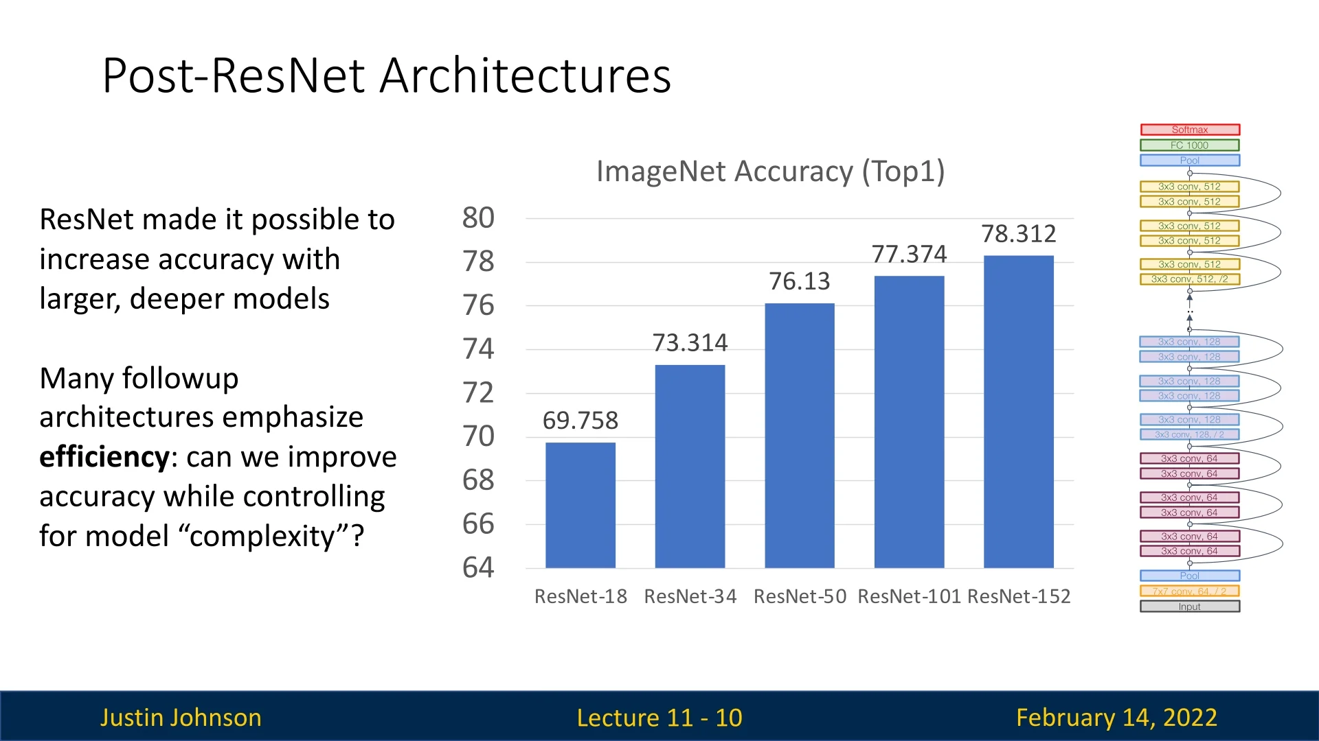
ResNet revolutionized deep learning by making it feasible to train much deeper models while maintaining high accuracy. However, increasing the depth indefinitely is not always practical due to computational constraints. Many subsequent architectures aim to improve accuracy while optimizing for computational efficiency. The goal is to maintain or surpass ResNet’s performance while controlling model complexity.
Model complexity can be measured in several ways:
- 1.
- Number of Parameters: The total number of learnable parameters in the model.
- 2.
- Floating Point Operations (FLOPs): The number of arithmetic
operations required for a single forward pass. This metric has subtle
nuances:
- Some papers count only operations in convolutional layers and ignore activation functions, pooling, and Batch Normalization.
- Many sources, including Justin’s notation, define “1 FLOP” as “1 multiply and 1 addition.” Thus, a dot product of two \(N\)-dimensional vectors requires \(N\) FLOPs.
- Other sources, such as NVIDIA, define a multiply-accumulate (MAC) operation as 2 FLOPs, meaning a dot product of two \(N\)-dimensional vectors takes \(2N\) FLOPs.
- 3.
- Network Runtime: The actual time taken to perform a forward pass on real hardware.
11.2 Grouped Convolutions
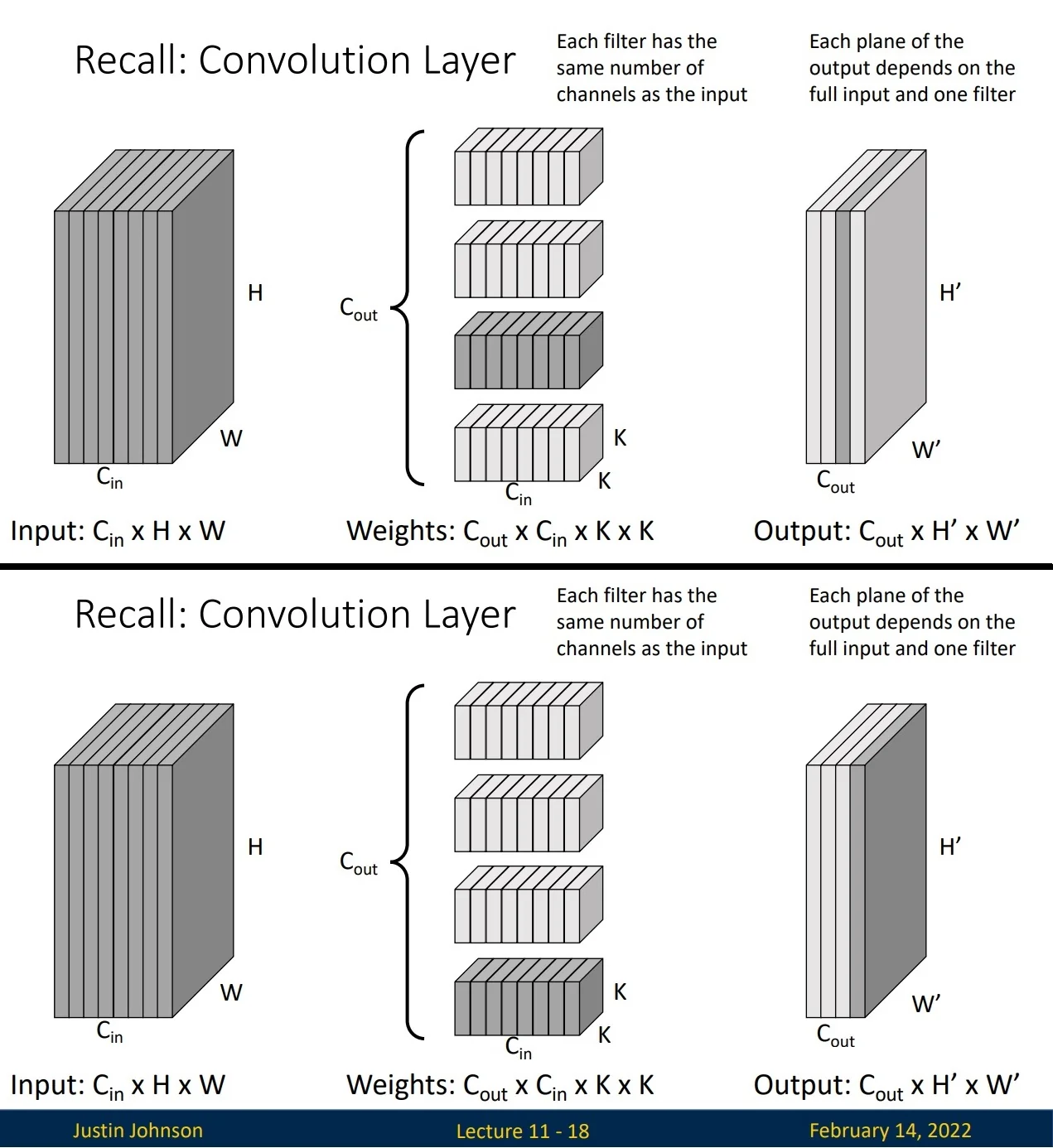
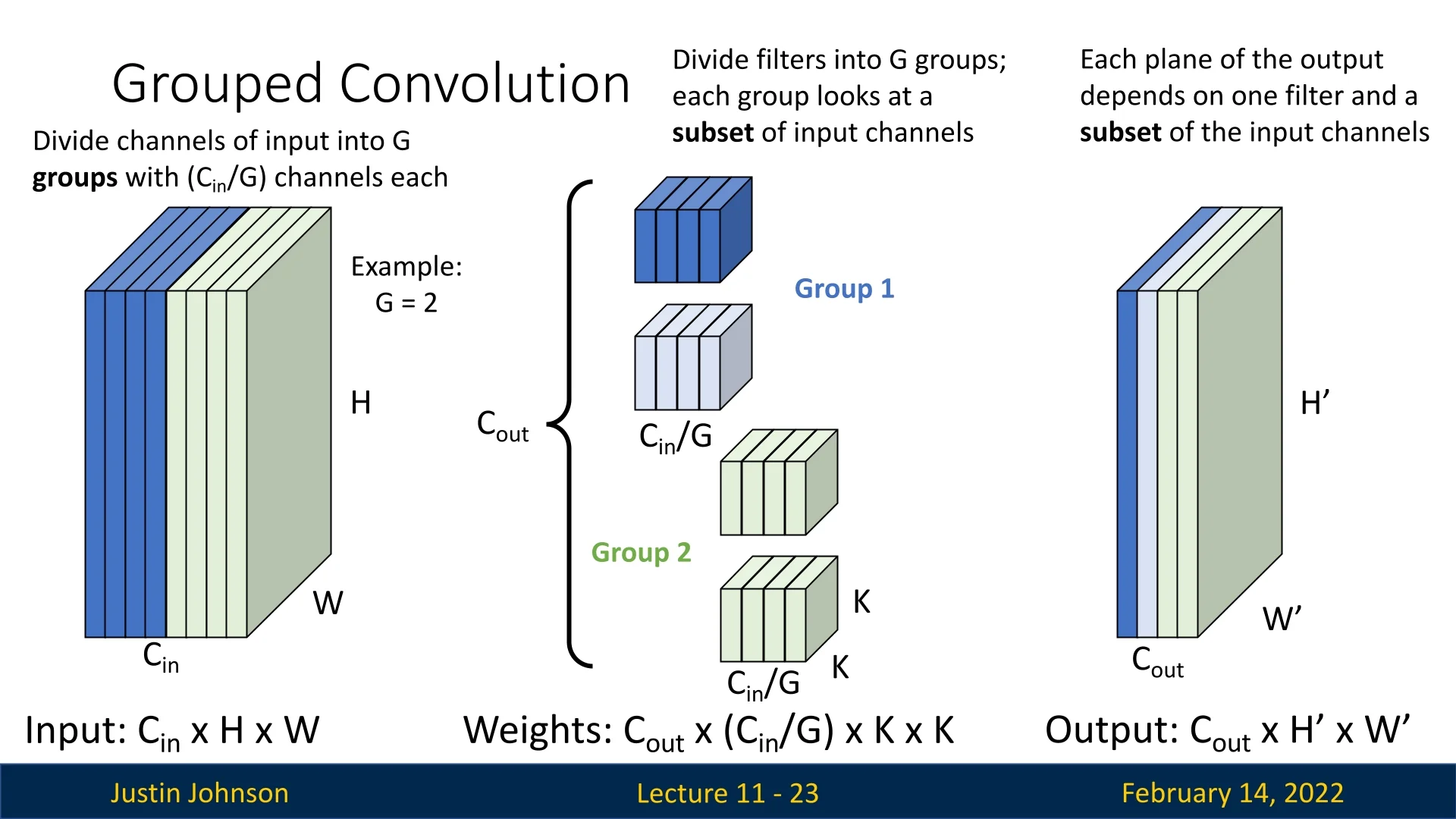
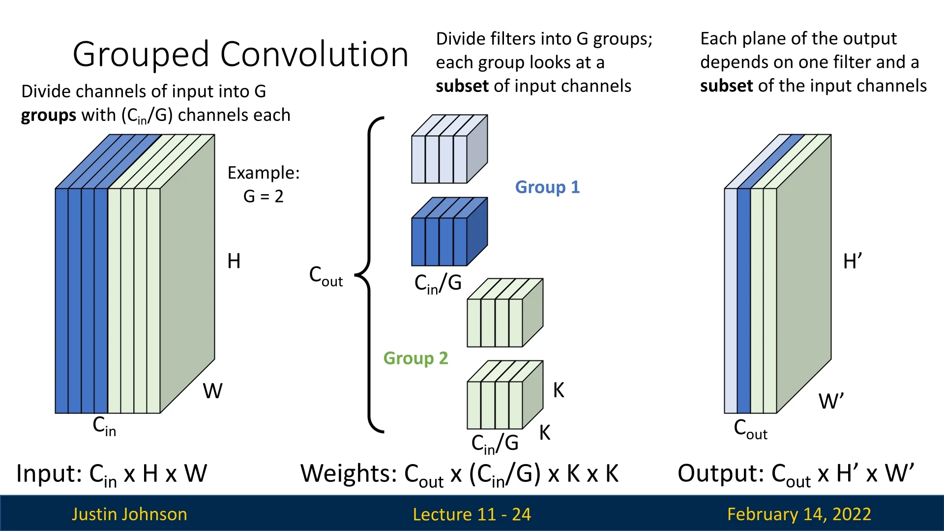
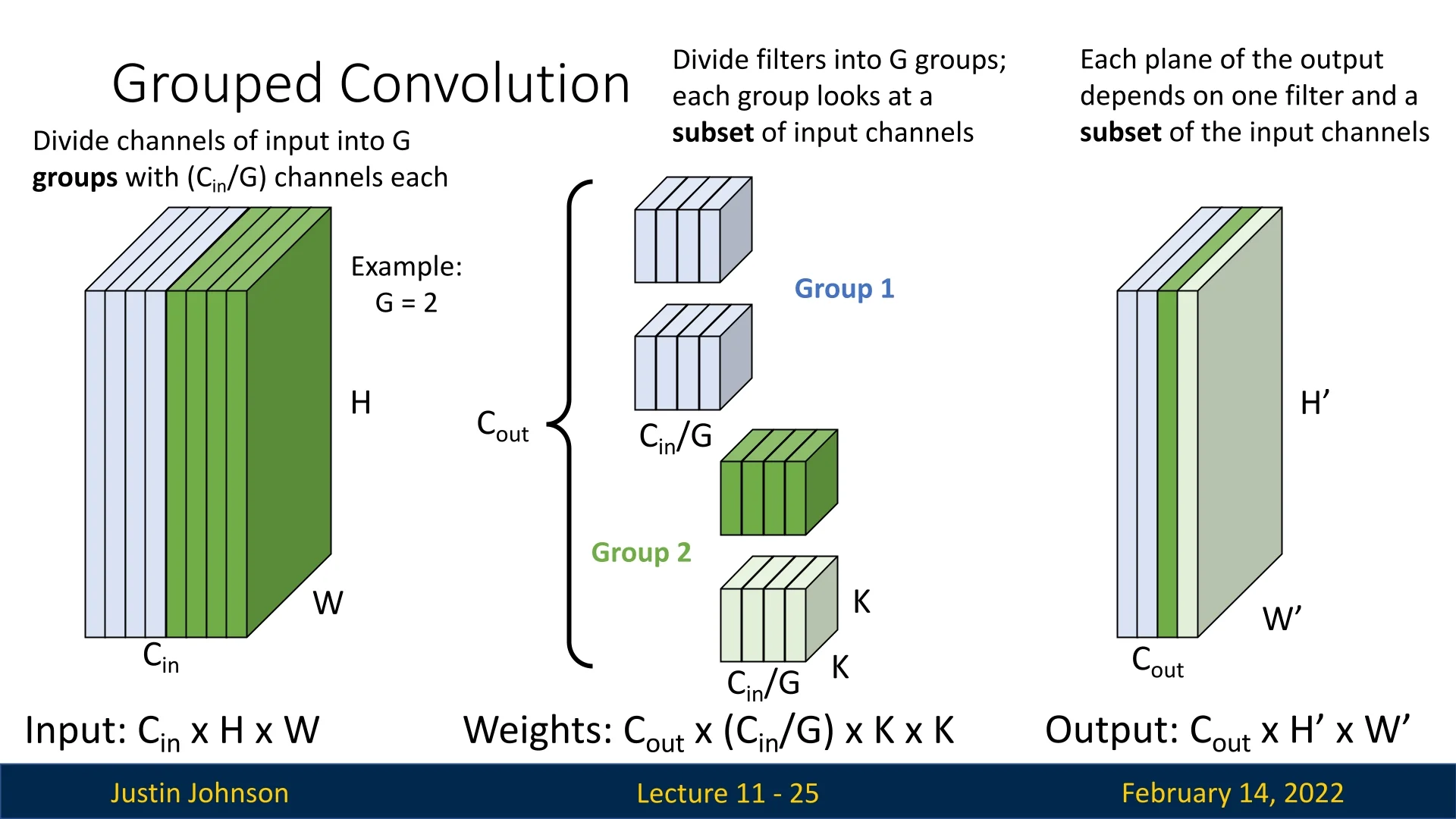
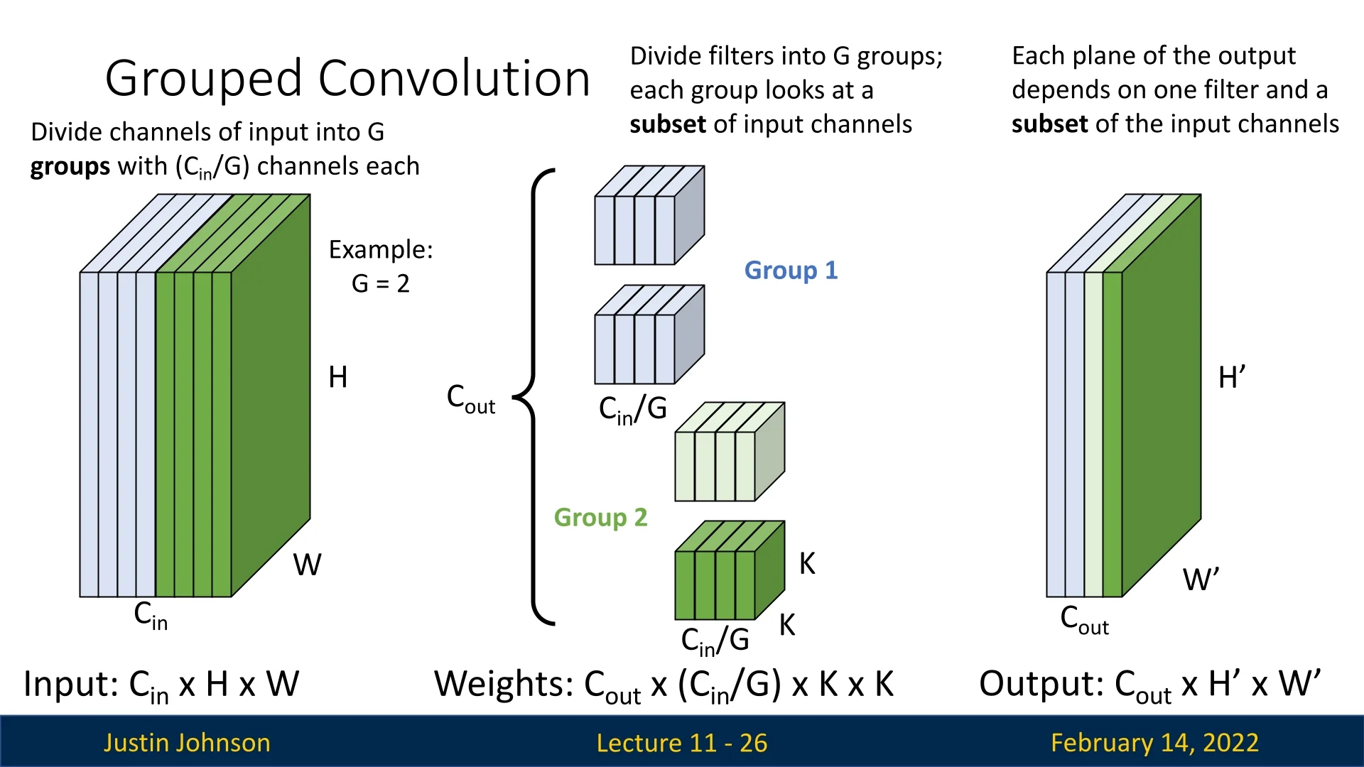
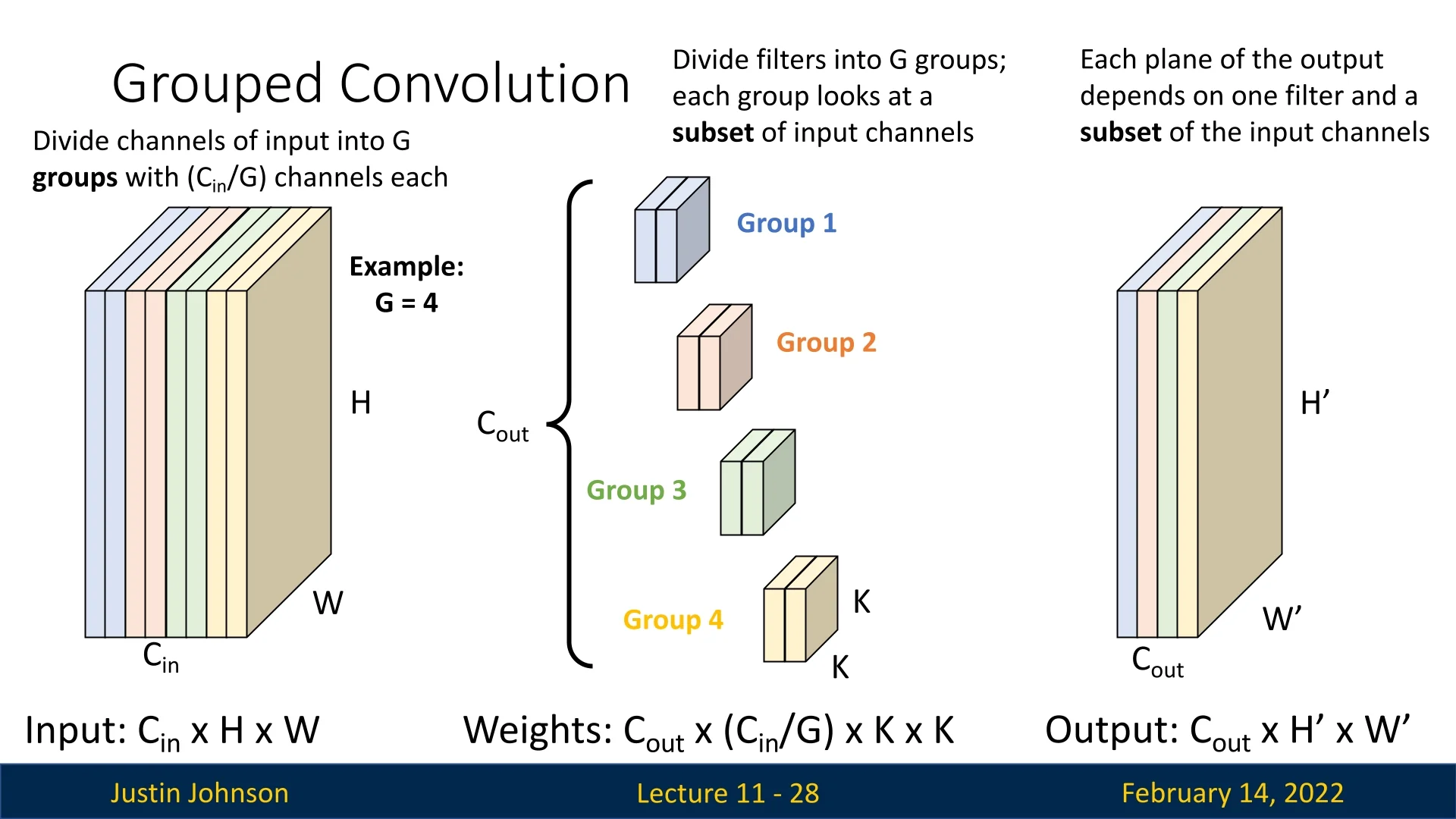
Before introducing grouped convolutions, let us recall the structure of standard convolutions. In a conventional convolutional layer:
- Each filter has the same number of channels as the input.
- Each plane of the output depends on the entire input and one filter.
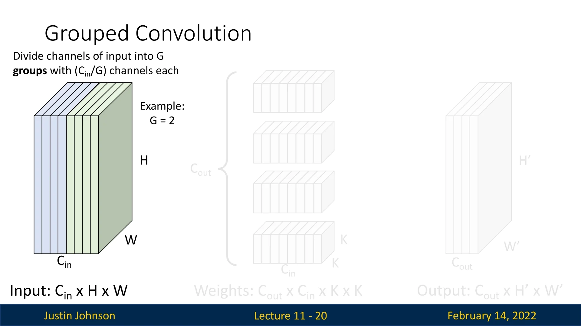
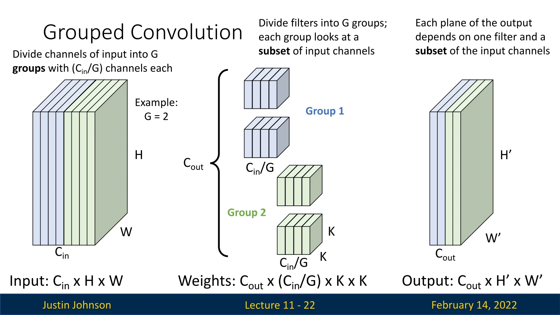
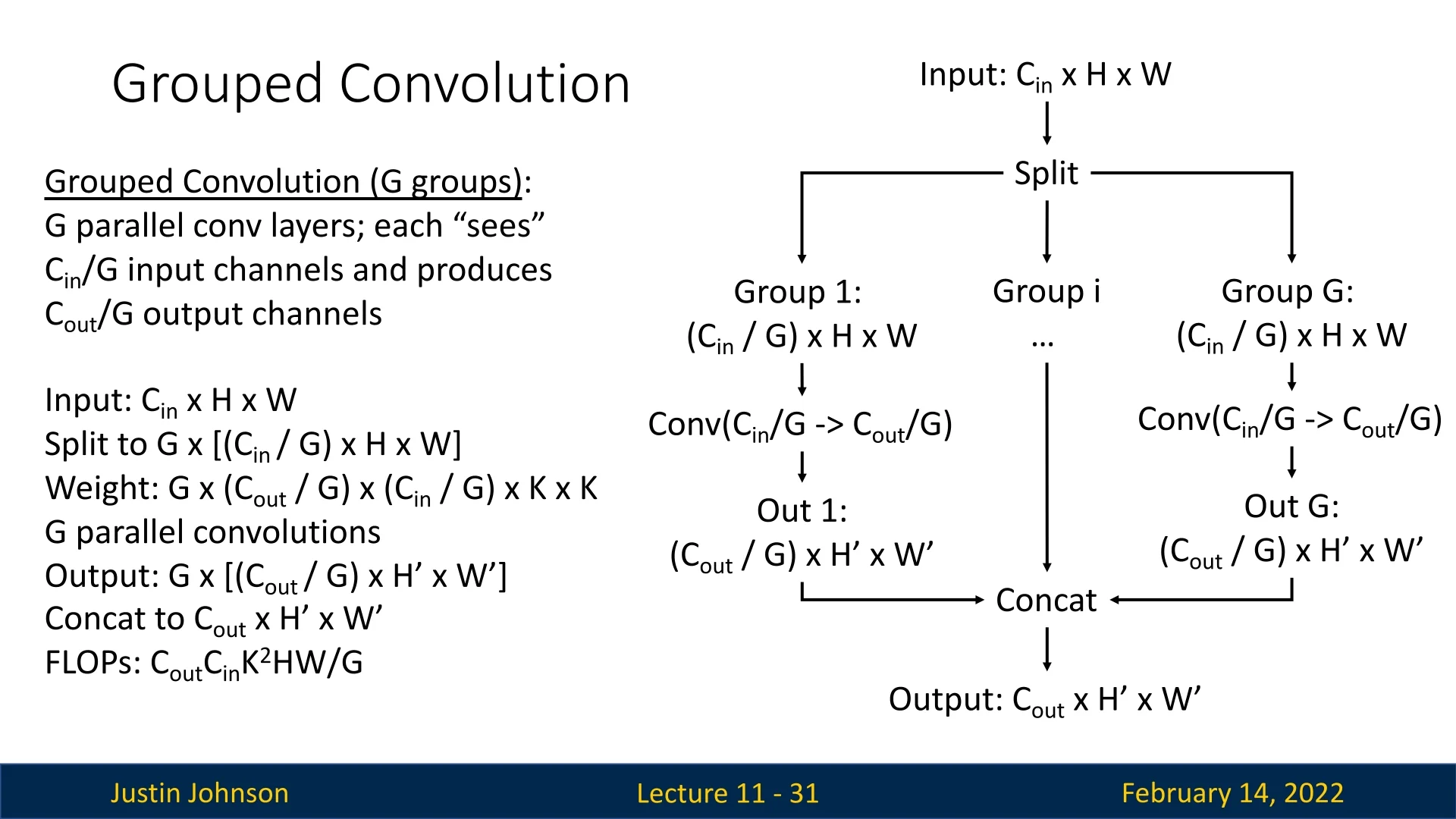
In grouped convolutions, we divide the input channels into \(G\) groups, where \(G\) is a hyperparameter. Each group consists of \(C_{in} / G\) channels.
- Each filter only operates on a specific subset of input channels corresponding to its group.
- The filters are divided into \(G\) groups, similar to input channels.
- The resulting weight tensor has dimensions: \(C_{out} \times (C_{in}/G) \times K \times K\).
Each output feature map now depends only on a subset of the input channels. Each group of filters produces \(C_{out}/G\) output channels.
We can visualize the process step by step:
This concept generalizes for any \(G > 1\). Below is an example where \(G=4\):
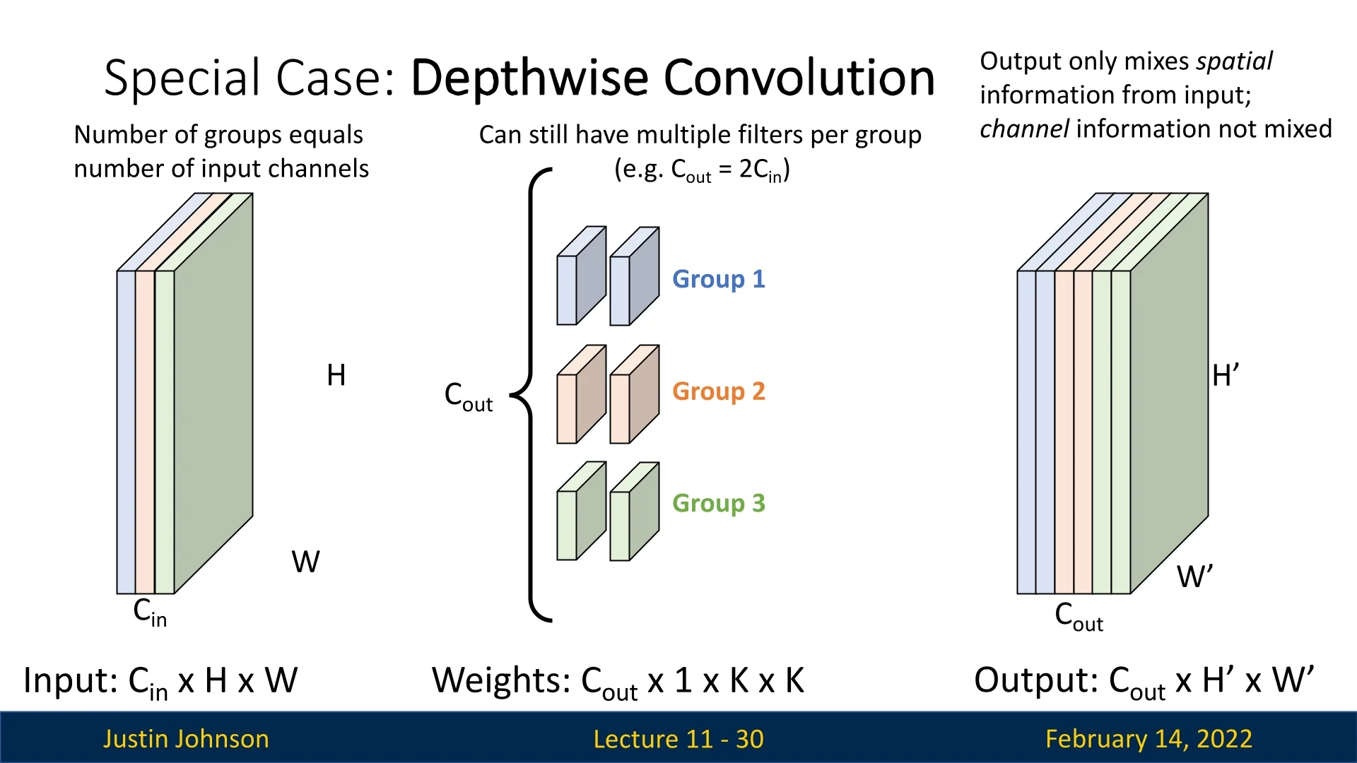
A special case of grouped convolutions that we’ve already encountered is depthwise convolution, where \(G\) is set to be equal to the number of input channels. In this scenario:
- Each filter operates on only one input channel.
- Output feature maps only mix spatial information but do not mix channel information.
Using grouped convolutions significantly reduces computational cost, making them an effective tool for designing efficient deep learning models.
11.2.1 Grouped Convolutions in PyTorch
Grouped convolutions can be efficiently implemented in PyTorch using the groups parameter in torch.nn.Conv2d. By default, groups=1, which corresponds to standard convolution where each filter processes all input channels. Setting groups > 1 splits the input channels into \(G\) groups, each processed by independent convolutional filters.
Below is an example demonstrating how to define grouped convolutions in PyTorch:
import torch
import torch.nn as nn

# Standard convolution (groups=1)
conv_standard = nn.Conv2d(in_channels=64, out_channels=128, kernel_size=3, padding=1, groups=1)

# Grouped convolution with G=2 (splitting input into 2 groups)
conv_grouped = nn.Conv2d(in_channels=64, out_channels=128, kernel_size=3, padding=1, groups=2)

# Depthwise convolution (each input channel has its own filter)
conv_depthwise = nn.Conv2d(in_channels=64, out_channels=64, kernel_size=3, padding=1, groups=64)

# Forward pass with a random input tensor
x = torch.randn(1, 64, 224, 224)  # Batch size of 1, 64 input channels, 224x224 image
output_standard = conv_standard(x)
output_grouped = conv_grouped(x)
output_depthwise = conv_depthwise(x)

print(f"Standard Convolution Output Shape: {output_standard.shape}")
print(f"Grouped Convolution Output Shape: {output_grouped.shape}")
print(f"Depthwise Convolution Output Shape: {output_depthwise.shape}")
Running this code will produce the following output:
Standard Convolution Output Shape: torch.Size([1, 128, 224, 224])
Grouped Convolution Output Shape: torch.Size([1, 128, 224, 224])
Depthwise Convolution Output Shape: torch.Size([1, 64, 224, 224])
Key Observations
-
Standard Convolution (\(groups=1\)):
- Each filter operates across all input channels.
- Computational cost remains high.
- The output has 128 channels, same as the number of filters.
-
Grouped Convolution (\(groups=G\)):
- The input channels are divided into \(G\) groups, with each group processed by independent filters.
- Computational cost is reduced by a factor of \(G\), making it more efficient.
- The output still has 128 channels, despite reducing computation.
-
Depthwise Convolution (\(groups=C_{in}\)):
- Each input channel has its own dedicated filter.
- Spatial information is mixed, but channel-wise information is not combined.
- The output has the same number of channels as the input (\(C_{in} = C_{out}\)).
When to Use Grouped Convolutions?
- Efficient Model Architectures: Used in models such as ResNeXt and Xception, to balance computational cost and accuracy.
- Reducing Computation in Large Networks: Splitting channels into groups significantly reduces FLOPs, making inference faster.
- Specialized Feature Learning: Each group can learn specialized features independently, improving representation learning.
Grouped convolutions, especially when combined with bottleneck layers and pointwise convolutions, allow for high-performance networks with significantly reduced computational costs.
11.3 ResNeXt: Next-Generation Residual Networks
ResNeXt, introduced by Microsoft Research in 2017 [730], builds upon ResNet’s foundation by incorporating aggregated residual transformations, utilizing multiple parallel pathways within residual blocks. This approach improves accuracy while maintaining computational efficiency, making it a more scalable and flexible architecture.
11.3.1 Motivation: Why ResNeXt?
Despite the success of ResNet, deeper and wider networks come with increased computational costs. Simply increasing depth does not always yield better performance due to optimization challenges, diminishing returns, and increased memory requirements. While widening the network (increasing the number of channels per layer) can improve capacity, it significantly increases FLOPs, making the model inefficient.
ResNeXt introduces a third dimension, cardinality (\(G\)), which refers to the number of parallel pathways in a residual block. Instead of solely increasing depth or width, ResNeXt adds multiple transformation pathways within a single block. The results are then concatenated together to a single output for the block. This allows for higher representational power without increasing the number of FLOPs, hence, without greatly increasing the computational cost.
11.3.2 Key Innovation: Aggregated Transformations
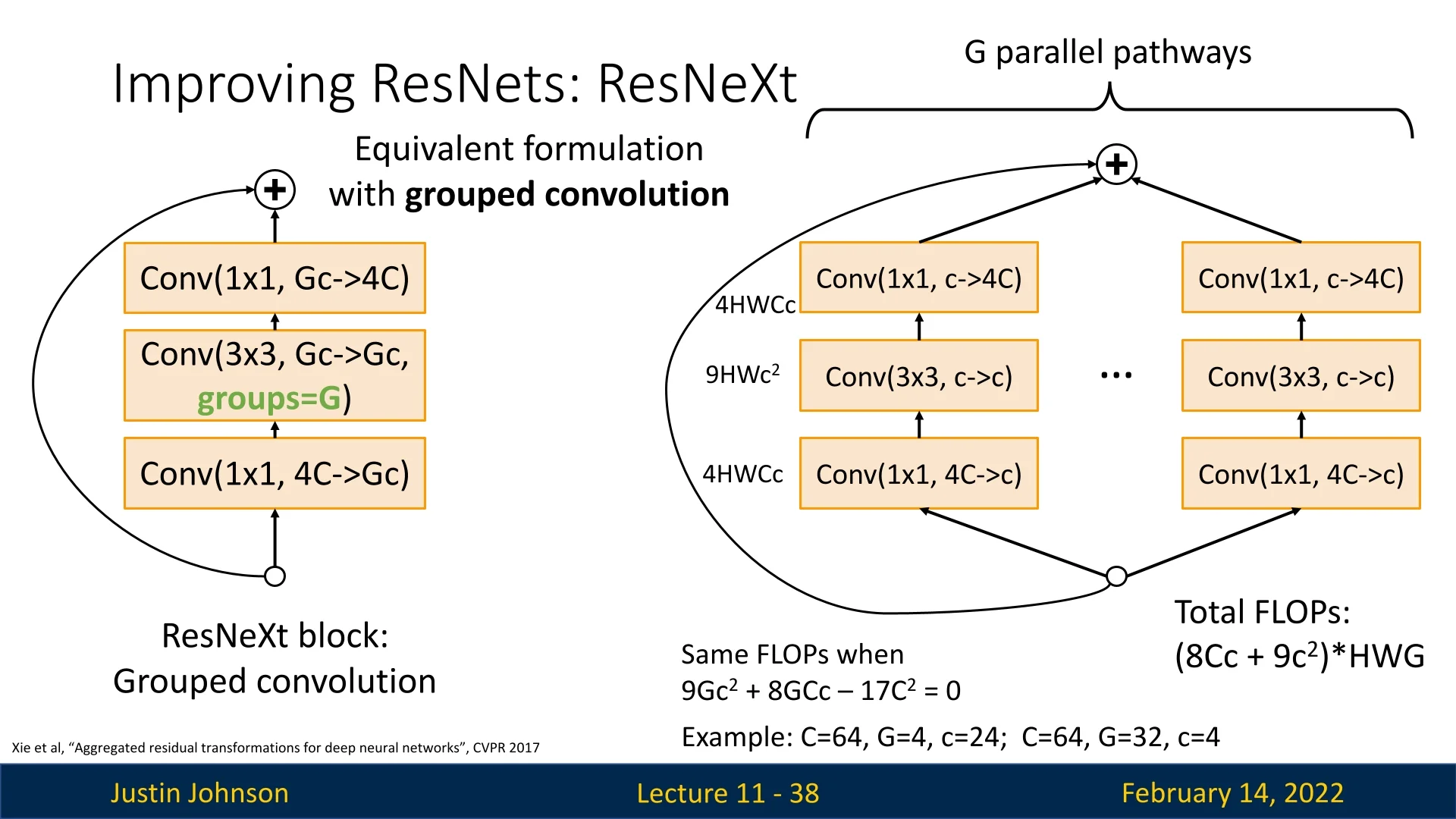
The key innovation in ResNeXt is the use of G parallel pathways of residual transformations. The original bottleneck block in ResNet consists of:
- A \(1\times 1\) convolution to reduce dimensionality (\(4C \to C\)), costing \(4HWC^2\) FLOPs.
- A \(3\times 3\) convolution (\(C \to C\)), costing \(9HWC^2\) FLOPs.
- A \(1\times 1\) convolution to restore dimensionality (\(C \to 4C\)), costing another \(4HWC^2\) FLOPs.
This totals to \(17HWC^2\) FLOPs per block.
ResNeXt modifies this by introducing G parallel pathways, each containing an intermediate channel count \(c\): \begin {equation} \mbox{FLOPs per pathway} = (8Cc + 9c^2)HW \end {equation} Summing over \(G\) pathways results in: \begin {equation} \mbox{Total FLOPs} = (8Cc + 9c^2)HWG \end {equation}
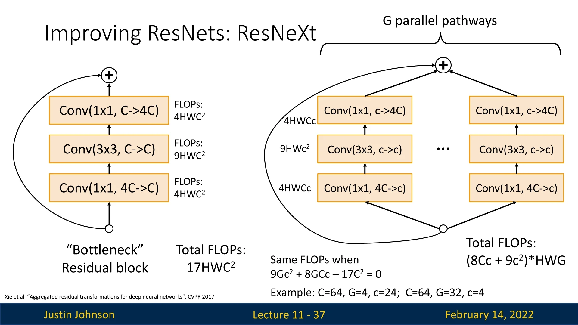
To maintain the same computational cost, we solve: \begin {equation} 9Gc^2 + 8GCc - 17C^2 = 0 \end {equation} Example solutions:
- \(C=64, G=4, c=24\)
- \(C=64, G=32, c=4\)
Therefore, with ResNeXt blocks, we now have the freedom to play with values of \(C,G,c\), and as long as the values solve the equation: \(9Gc^2 + 8GCc - 17C^2 = 0\), enjoy from different architectures with the same computational cost (i.e., the same number of FLOPs).
From testing it empirically, it appears that we can use this argument, and that by increasing the number of groups (\(G\)) while concurrently reducing the group width, we can improve performance while preserving the number of FLOPs.
11.3.3 ResNeXt and Grouped Convolutions
ResNeXt’s implementation can also be formulated in terms of grouped convolutions, making it easy to construct them in practice. Instead of explicitly creating multiple transformation pathways, we use grouped convolutions to enforce this structure efficiently.
Each ResNeXt block is structured as:
- \(1\times 1\) convolution (\(4C \to Gc\))
- \(3\times 3\) grouped convolution (\(Gc \to Gc\), groups=G)
- \(1\times 1\) convolution (\(Gc \to 4C\))
11.3.4 Advantages of ResNeXt Over ResNet
ResNeXt builds upon the ResNet design by introducing a structured, multi-pathway architecture that enhances representational power without incurring significant additional computational cost.
To summarize, ResNeXt’s key advantages over ResNet include:
- Improved Accuracy: The additional parallel transformation pathways enable richer feature extraction, leading to higher accuracy.
- Enhanced Efficiency: Instead of merely increasing network depth or width, ResNeXt uses grouped convolutions (parameterized by \(G\)) to boost capacity efficiently, outperforming deeper or wider ResNets at a similar computational cost.
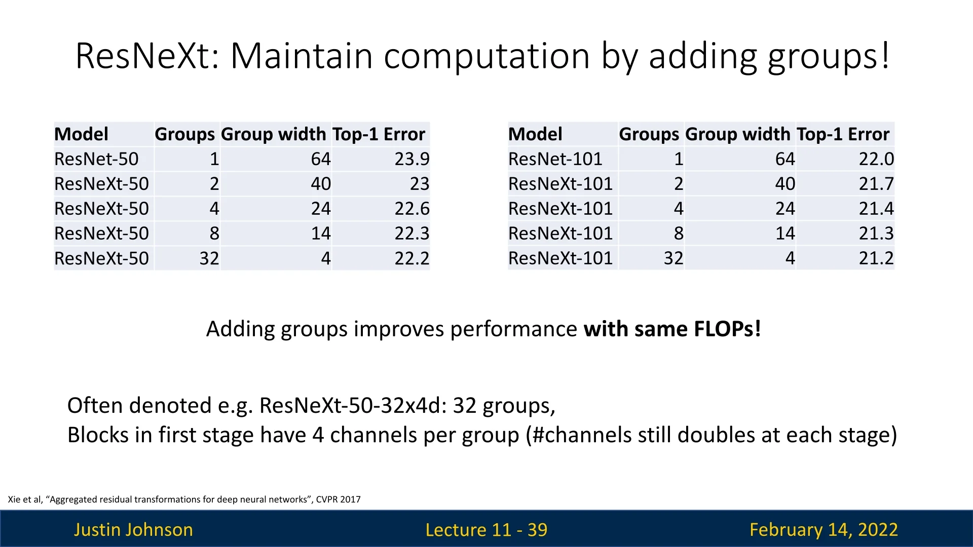
11.3.5 ResNeXt Model Naming Convention
ResNeXt models are typically denoted as ResNeXt-50-32x4d, where:
- 50: Number of layers.
- 32: Number of groups (\(G\)).
- 4: Number of intermediate channels (dimensions) per group.
ResNeXt’s design principles went on to influence many later architectures, shaping how modern networks balance efficiency and expressiveness. Its core idea of aggregated transformations—splitting a feature map into parallel low-dimensional paths, transforming them independently, and then merging the results—proved broadly applicable beyond residual networks. This concept of scalable parallelism inspired the development of subsequent families of models that sought to improve performance not by simply increasing depth or width, but by refining how computations are organized. Later architectures such as EfficientNet and Vision Transformers (ViTs), which will be discussed in later chapters, extend this idea in different forms: one through highly efficient grouped and depthwise operations, and the other through parallel multi-head transformations. In both cases, the underlying philosophy introduced by ResNeXt—that richer representations can emerge from multiple lightweight, independent transformations rather than a single monolithic one—became a lasting design pattern across deep learning.
11.4 Squeeze-and-Excitation Networks (SENet)
In 2017, researchers expanded upon ResNeXt by introducing Squeeze-and-Excitation Networks (SENet), which introduced a novel Squeeze-and-Excitation (SE) block [244]. The core idea behind SENet was to incorporate global channel-wise attention into ResNet blocks, improving the model’s ability to capture interdependencies between channels. This enhancement led to improved classification accuracy while adding minimal computational overhead.
SENet won first place in the ILSVRC 2017 classification challenge, achieving a top-5 error rate of 2.251%, a remarkable 25% relative improvement over the winning model of 2016.
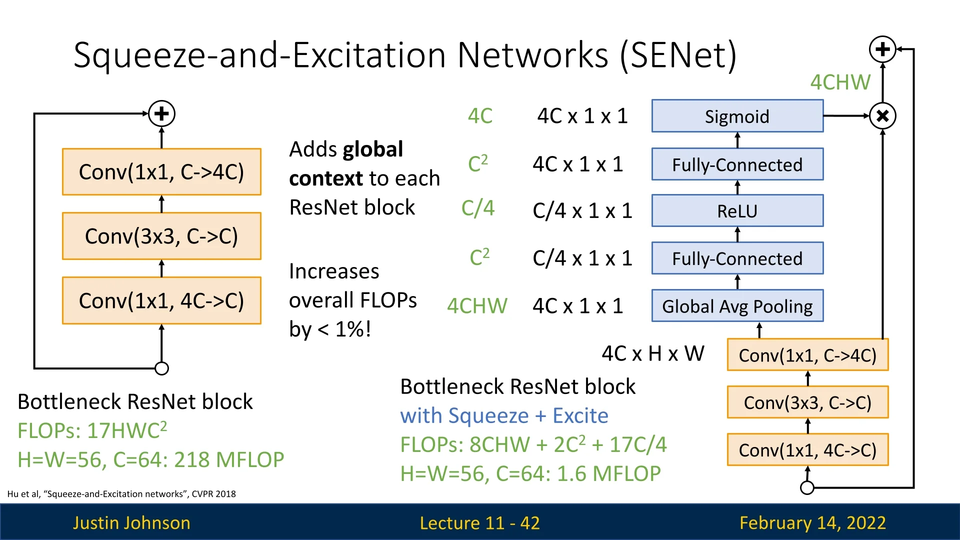
11.4.1 Squeeze-and-Excitation (SE) Block
The SE block is designed to enhance the representational power of convolutional networks by introducing a channel-wise attention mechanism. Instead of treating all channels equally, SE blocks allow the network to dynamically recalibrate the importance of different feature channels by learning their global interdependencies.
In standard convolutional layers, feature maps are processed independently across channels, meaning each filter learns to extract spatial patterns without directly considering how different feature channels relate to one another. The SE block addresses this limitation by introducing a two-step process: Squeeze and Excitation.
Squeeze: Global Information Embedding
Each convolutional layer in a ResNet bottleneck block produces a set of feature maps, where each channel captures different aspects of the input. However, these feature maps primarily focus on local spatial information, meaning that each activation in a feature map is computed independently of global image context.
To address this, the squeeze operation applies global average pooling across all spatial locations, condensing the entire spatial feature representation into a compact channel descriptor. This descriptor captures global context, summarizing the overall activation strength for each channel: \begin {equation} z_c = \frac {1}{H \times W} \sum _{i=1}^{H} \sum _{j=1}^{W} U_c(i,j) \end {equation} where:
- \(U_c(i,j)\) is the activation at spatial position \((i,j)\) for channel \(c\).
- \(z_c\) is a single scalar that represents the global response of channel \(c\).
This operation transforms each feature map from a spatial feature map of shape \((H, W)\) into a single scalar value, providing a compact summary of the channel’s overall importance.
Excitation: Adaptive Recalibration
While the squeeze operation extracts global statistics, it does not yet provide a mechanism for adjusting the importance of each channel. The excitation step models channel-wise dependencies by learning how much each channel should contribute to the final representation.
The excitation process consists of two fully connected (FC) layers, followed by a sigmoid activation: \begin {equation} s = \sigma (W_2 \delta (W_1 z)) \end {equation} where:
- \(W_1 \in \mathbb {R}^{C/r \times C}\) and \(W_2 \in \mathbb {R}^{C \times C/r}\) are learnable weight matrices.
- \(\delta \) is the ReLU activation function.
- \(\sigma \) is the sigmoid activation function, ensuring that each recalibration weight is in the range \((0,1)\).
- \(r\) is the reduction ratio, a hyperparameter controlling the dimensionality bottleneck.
Channel Recalibration
The output of the excitation function is a set of learned channel-wise scaling factors \(s = [s_1, s_2, ..., s_C]\), where each \(s_c\) determines how important the corresponding channel \(c\) is. These learned scalars are applied to the original feature maps using channel-wise multiplication: \begin {equation} \tilde {U}_c = s_c \cdot U_c \end {equation} where each feature map is rescaled according to its learned importance. Channels with high \(s_c\) values are emphasized, while those with low values are suppressed.
How SE Blocks Enhance ResNet Bottleneck Blocks
SE blocks are an additional component that can be inserted into any convolutional block. In ResNet’s bottleneck block, SE is added before the final summation with the shortcut connection. The process can be summarized as follows:
- 1.
- The input feature maps pass through the standard bottleneck
transformation:
- \(1 \times 1\) convolution reduces dimensions (\(4C \to C\)).
- \(3 \times 3\) convolution extracts spatial features (\(C \to C\)).
- \(1 \times 1\) convolution restores dimensions (\(C \to 4C\)).
- 2.
- Instead of immediately proceeding to the residual summation, the feature
maps are processed by an SE block:
- Global average pooling (squeeze) reduces each feature map to a scalar.
- Two fully connected layers (excitation) learn per-channel importance.
- The feature maps are reweighted based on their learned importance.
- 3.
- The recalibrated feature maps are passed to the identity shortcut connection and summed, completing the residual connection.
Why Does SE Improve Performance?
- Improved Feature Selection: SE blocks enable the network to focus on the most relevant channels, reducing noise and improving discrimination.
- Global Context Awareness: By incorporating global average pooling, the model learns to adjust features based on the entire input, rather than relying solely on local spatial filters.
-
Minimal Computational Overhead: Adding SE blocks increases FLOPs only marginally (usually by less than 1%). For example, in a ResNet bottleneck block:
- Without SE: \(17HWC^2\) FLOPs.
- With SE: \(8CHW + 2C^2 + \frac {17}{4}C\) FLOPs.
For \(H=W=56, C=64\), this translates to an increase from 218 MFLOPs to 219.6 MFLOPs.
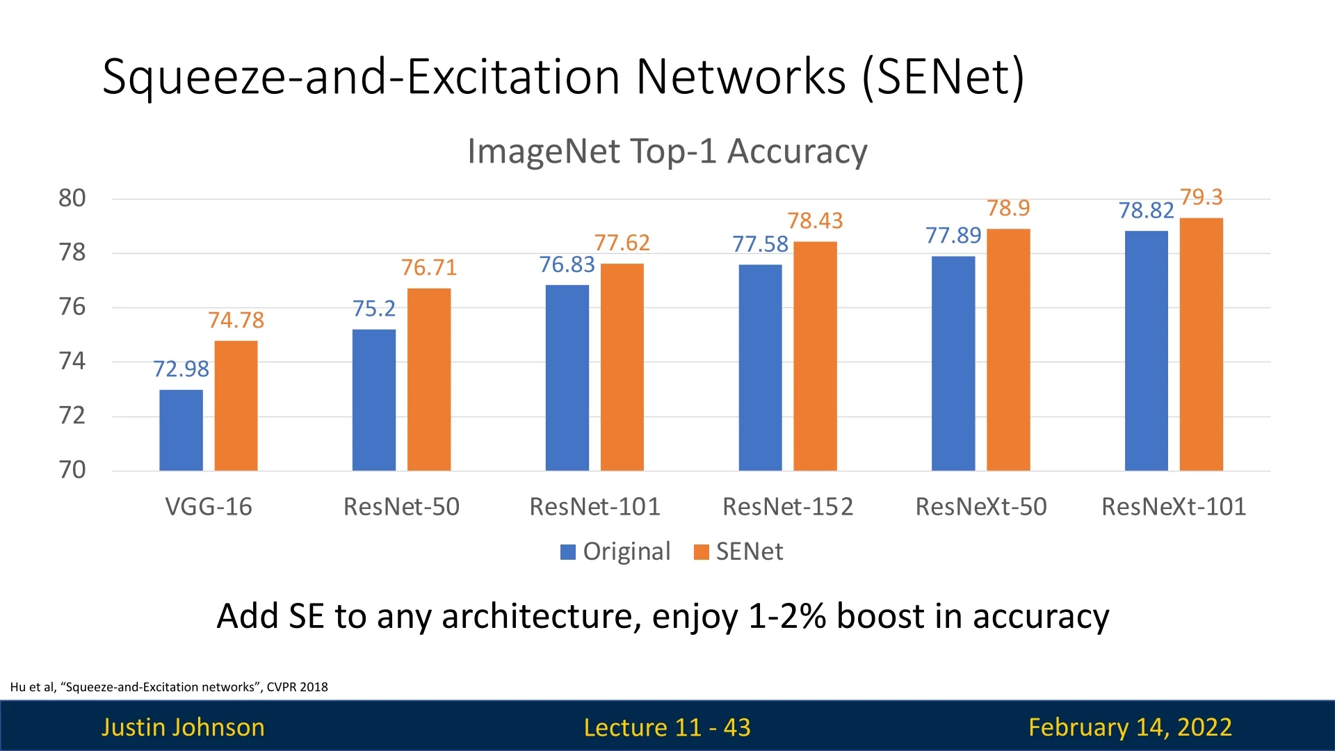
Performance Gains, Scalability, and Integration of SE Blocks
Incorporating SE blocks consistently improves accuracy across various architectures. By introducing dynamic channel-wise attention, SE blocks enable CNNs to focus on the most relevant features, improving feature discrimination without significant computational overhead.
Impact on Various Tasks
SE blocks enhance performance across multiple domains:
- Image Classification: SE-ResNet-50 achieves a top-5 error of 6.62% compared to 7.48% for ResNet-50. Similar improvements occur in SE-ResNet-101, SE-ResNeXt-50, and SE-Inception-ResNet-v2.
- Object Detection: Integrating SE into Faster R-CNN with a ResNet-50 backbone improves average precision by 1.3% on COCO, a relative gain of 5.2%.
- Scene Classification: SE-ResNet-152 reduces the Places365 top-5 error from 11.61% to 11.01%.
Practical Applications and Widespread Adoption
Due to their efficiency and adaptability, SE blocks have been widely integrated into many advanced architectures beyond classification:
- Object Detection: Faster R-CNN and RetinaNet benefit from SE-enhanced backbone networks.
- Semantic Segmentation: DeepLab and U-Net architectures integrate SE blocks to improve feature selection.
- Lightweight Models: MobileNet and ShuffleNet variants incorporate SE blocks, enhancing feature discrimination without significantly increasing computation.
SE blocks thus serve as a general-purpose enhancement that improves accuracy across diverse architectures and applications with minimal computational trade-offs.
11.4.2 SE Blocks and the End of the ImageNet Classification Challenge
The introduction of SE blocks in 2017 marked a turning point in the history of deep learning for image classification. With the Squeeze-and-Excitation Network (SENet) winning the ILSVRC 2017 classification challenge by a significant margin, the ImageNet competition had effectively reached its saturation point. The classification problem that had driven progress in convolutional neural networks (CNNs) for years was, metaphorically, squeezed to a pulp.
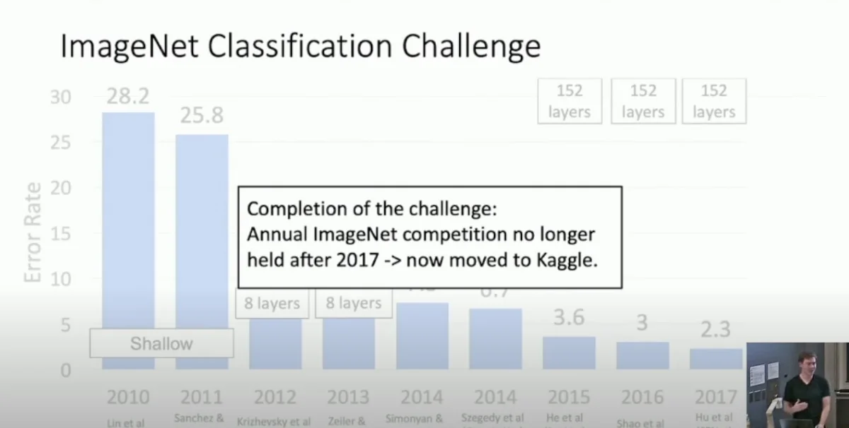
With SENet achieving a top-5 error rate of 2.251%, nearly matching human-level performance on ImageNet, it became clear that further improvements in classification accuracy would yield diminishing returns. The focus of research started shifting away from pure classification improvements and toward efficiency, enabling CNNs to be deployed on real-world devices.
11.4.3 Challenges and Solutions for SE Networks
Challenges of SE Networks
While Squeeze-and-Excitation (SE) blocks offer performance improvements, they introduce certain limitations that can impact their effectiveness in deep learning architectures:
- Loss of Spatial Information: Since SE blocks operate exclusively on channel-wise statistics, they ignore spatial relationships between pixels. This is particularly problematic for tasks requiring fine-grained spatial awareness, such as semantic segmentation or object detection.
- Increased Computational Cost: The excitation step involves two fully connected layers, introducing additional parameters and increasing inference time, which can be a concern in real-time applications or mobile deployments.
- Feature Over-suppression: If the learned channel-wise attention weights are improperly calibrated, they may suppress essential features, degrading model performance by eliminating useful information.
Solutions to SE Network Challenges
To address these challenges, several modifications and enhancements have been proposed:
- Combining SE with Spatial Attention: To mitigate the loss of spatial information, SE blocks can be integrated with spatial attention mechanisms, such as CBAM (Convolutional Block Attention Module) [720], which applies both channel-wise and spatial attention to improve feature selection. We will explore attention mechanisms in more detail in a later part of the course.
- Lightweight Excitation Mechanisms: The computational cost of SE blocks can be reduced by using depthwise separable convolutions instead of fully connected layers, as demonstrated in MobileNetV3 [240]. This allows for efficient feature recalibration without a significant increase in parameters.
- Normalization-Based Calibration: Applying normalization techniques, such as BatchNorm or GroupNorm, in the excitation step can help stabilize activations and prevent over-suppression of important features, leading to more balanced feature scaling.
Despite these challenges, SE blocks remain a widely used technique for enhancing neural network performance, particularly in mobile architectures where efficiency and accuracy need to be balanced carefully.
Shifting Research Directions: Efficiency and Mobile Deployability
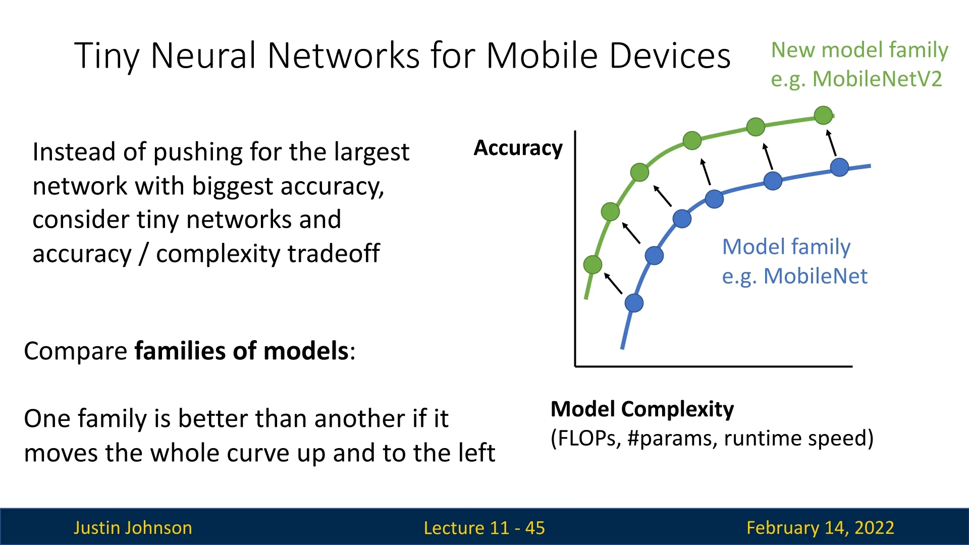
While deeper and more powerful models like SENet were being developed, practical applications demanded lightweight and efficient networks that could run on resource-constrained devices such as mobile phones, embedded systems, and edge devices. This need led to a new era of model design, emphasizing:
- Reducing computational complexity while maintaining accuracy.
- Optimizing models for mobile and embedded hardware (e.g., efficient CNN architectures).
- Exploring new paradigms beyond conventional CNN-based feature extraction.
What Comes Next?
In the following sections, we will explore some of the architectures that emerged as a response to these practical challenges:
- MobileNets: Depthwise separable convolutions for efficient mobile-friendly models.
- ShuffleNet: Grouped convolutions with channel shuffling to optimize computation.
- EfficientNet: Compound scaling of depth, width, and resolution to maximize accuracy per FLOP.
These models set the stage for efficient deep learning, shifting the paradigm from brute-force accuracy improvements to optimal model design for real-world deployment.
11.5 Efficient Architectures for Edge Devices
As deep learning models become increasingly powerful, their computational demands also rise sharply. Yet many real-world applications—such are running on smartphones or other embedded systems like in autonomous vehicles. In this section, we explore the evolution of CNN architectures designed for embedded systems, aiming to optimize the accuracy-to-FLOP ratio, striking a careful balance between computational efficiency and predictive performance.
The journey in efficient deep learning begins with MobileNets, which introduced depthwise separable convolutions to dramatically reduce computational cost while preserving competitive accuracy. Subsequent innovations, such as ShuffleNet, further improved efficiency by reorganizing channel connectivity. More recently, advanced models like EfficientNet have pushed the boundaries by jointly scaling network depth, width, and resolution. Competing architectures such as RegNet offer similar accuracy at the same FLOP level while achieving up to five times faster training speeds.
In the following subsections, we trace the development of these efficient architectures—from the early MobileNets and ShuffleNet to the latest EfficientNet and RegNet models—highlighting the key design principles and innovations that make them well-suited for deployment on edge devices.
11.5.1 MobileNet: Depthwise Separable Convolutions
MobileNetV1 was designed to create highly efficient neural networks that could run in real-time on low-power devices. The key innovation behind MobileNet is its use of Depthwise Separable Convolutions, which factorize a standard convolution operation into two separate steps:
- 1.
- A Depthwise Convolution, where a single convolutional filter is applied per input channel (instead of applying filters across all channels as in standard convolutions).
- 2.
- A Pointwise Convolution (\(1 \times 1\) convolution), which projects the depthwise output back into a full feature representation.
This decomposition significantly reduces the number of computations required while still maintaining sufficient expressiveness.
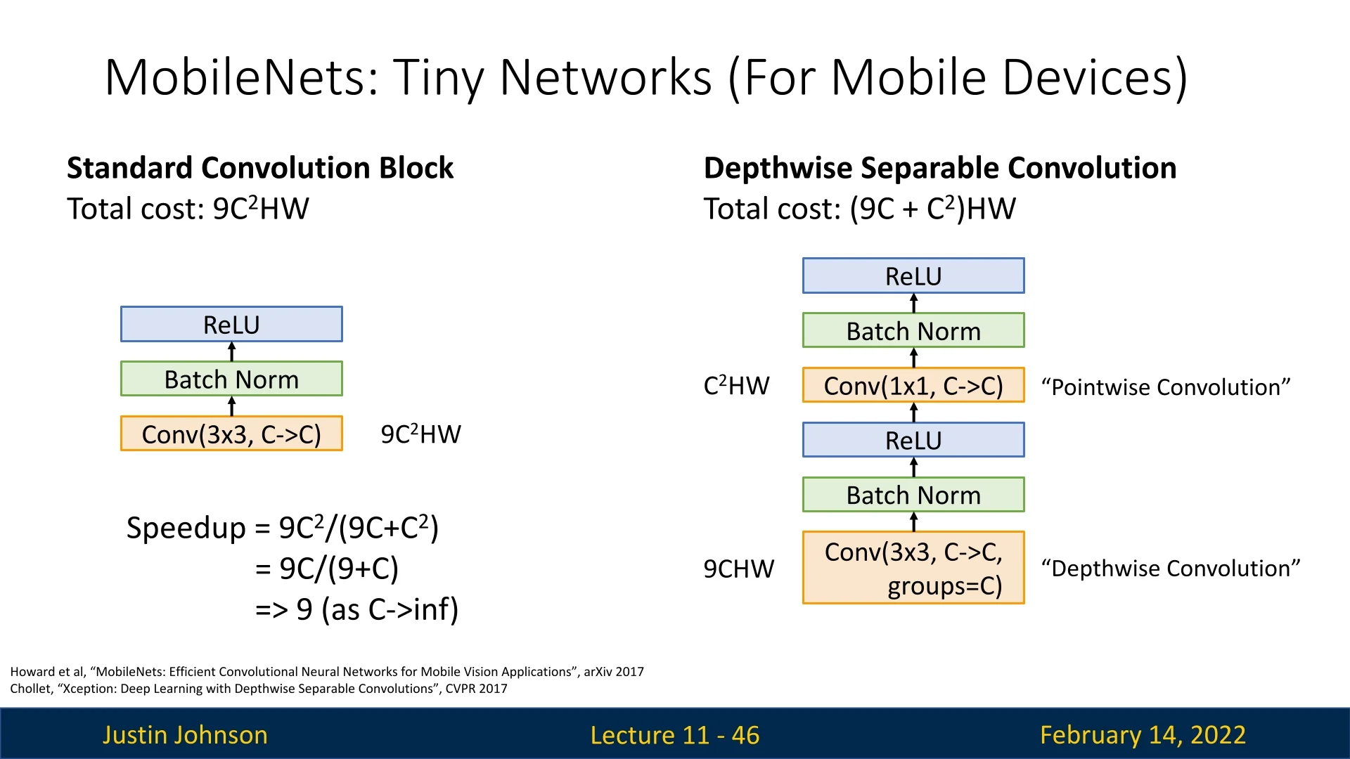
To understand the efficiency gain, consider the computational cost:
- Standard Convolution: \(9C^2HW\) FLOPs.
- Depthwise Separable Convolution: \((9C + C^2)HW\) FLOPs.
The speedup is given by: \begin {equation} \frac {9C^2}{9C + C^2} = \frac {9C}{9+C} \end {equation} As \(C \to \infty \), the speedup approaches 9\(\times \), demonstrating the substantial computational savings.
Width Multiplier: Thinner Models
A key parameter in MobileNet is the width multiplier \(\alpha \in (0,1]\). It uniformly scales the number of channels in each layer: \[ \mbox{(Input channels)} \;\mapsto \; \alpha \times (\mbox{Input channels}), \quad \mbox{(Output channels)} \;\mapsto \; \alpha \times (\mbox{Output channels}). \] When \(\alpha =1\), MobileNet uses the baseline channel sizes. As \(\alpha \) decreases, the network becomes thinner at every layer, reducing both computation and parameters approximately by \(\alpha ^2\). Typical choices include \(\alpha \in \{1, 0.75, 0.5, 0.25\}\), which trade off accuracy for efficiency in a predictable manner.
Resolution Multiplier: Reduced Representations
Another hyperparameter to control model size is the resolution multiplier \(\rho \in (0,1]\). It uniformly scales the spatial resolution at each layer: \[ \mbox{(Input height/width)} \;\mapsto \; \rho \times (\mbox{Input height/width}), \] and similarly for intermediate feature-map resolutions. Reducing resolution can shrink the FLOPs by approximately \(\rho ^2\). Common input resolutions are \(\{224,192,160,128\}\), corresponding to \(\rho = 1,\,0.86,\,0.71,\,0.57\) relative to \(224\times 224\).
Computational Cost of Depthwise Separable Convolutions
In MobileNet, each layer is a depthwise separable convolution, split into:
- 1.
- Depthwise Conv \((K \times K)\): One spatial filter per input channel.
- 2.
- Pointwise Conv \((1 \times 1)\): A standard convolution across all input channels to produce output channels.
If the baseline layer has \(\,M\) input channels, \(\,N\) output channels, kernel size \(K\!\times K\), and spatial dimension \(D\!\times D\), then the total FLOPs for a depthwise separable layer are: \[ \underbrace {(K \times K) \cdot M \cdot D^2}_{\mbox{Depthwise}} \;+\; \underbrace {(1 \times 1)\cdot M \cdot N \cdot D^2}_{\mbox{Pointwise}}. \] Applying the width multiplier \(\alpha \) and resolution multiplier \(\rho \) modifies the above to: \[ (K \times K)\,\cdot \,(\alpha M)\,\cdot \,(\rho D)^2 \;+\; (\alpha M)\,\cdot \,(\alpha N)\,\cdot \,(\rho D)^2, \] which can be written as: \[ (\rho D)^2 \bigl [ (K^2)\,\alpha M \;+\; \alpha ^2 (M \cdot N) \bigr ]. \] Hence, choosing smaller \(\alpha \) or \(\rho \) scales down the network’s computation and number of parameters, at the cost of some accuracy.
Summary of Multipliers Together, the width and resolution multipliers \((\alpha , \rho )\) provide a simple yet powerful mechanism to tailor MobileNet to a wide range of resource constraints, making it suitable for both high-performance and highly constrained edge-device environments.
MobileNetV1 vs. Traditional Architectures
Despite its lightweight design, MobileNetV1 achieves remarkable efficiency compared to traditional CNNs. Table 11.1 highlights a comparison on the ImageNet dataset.
MobileNet-224 achieves nearly the same accuracy as VGG-16 while using 97% fewer parameters and 96% fewer FLOPs, making it an ideal choice for real-time edge applications.
Depthwise Separable vs. Standard Convolutions in MobileNet
To understand the tradeoffs involved in using depthwise separable convolutions, the following table compares a regular convolutional MobileNet to one using depthwise separable convolutions.
The use of depthwise separable convolutions results in:
- A slight drop in accuracy (71.7% \(\to \) 70.6%).
- A 7\(\times \) reduction in parameters (29.3M \(\to \) 4.2M).
- A 9\(\times \) reduction in FLOPs (4866M \(\to \) 569M).
This tradeoff is highly favorable for edge applications where computational efficiency is critical.
Summary and Next Steps
MobileNetV1 demonstrated that Depthwise Separable Convolutions can drastically reduce computational cost while maintaining competitive accuracy. By factorizing a standard convolution into a 3×3 depthwise convolution (mixing spatial information) followed by a 1×1 pointwise convolution (mixing channel information), the model achieves significant efficiency gains.
However, a key limitation remains: the 1×1 pointwise convolution still operates on all channels uniformly. Since this convolution processes each channel independently before recombining them, there is room for optimization in how channels interact.
What’s the problem? The current design lacks an explicit mechanism to exchange information across different channels efficiently. Consider an alternative approach: grouped convolutions, which split channels into independent groups to reduce computational cost. While grouped convolutions lower the FLOP count, they introduce a new issue—channels within a group never interact with channels from other groups. This results in each output channel only depending on a limited subset of input channels, restricting the model’s capacity to learn rich feature representations.
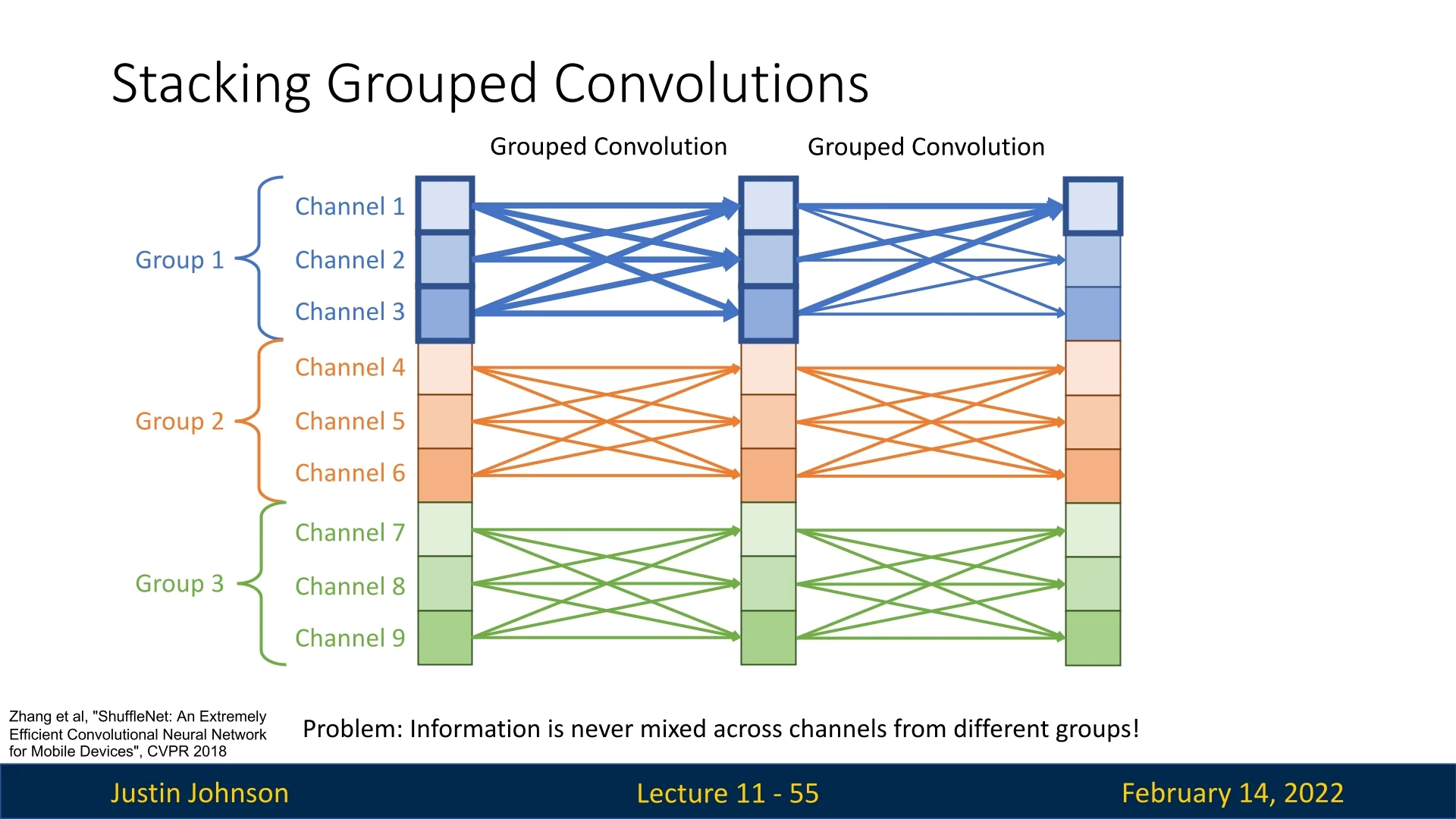
This observation raises a fundamental question: Can we mix channel information more efficiently while maintaining the computational benefits of grouped convolutions?
11.5.2 ShuffleNet: Efficient Channel Mixing via Grouped Convolutions
MobileNetV1 demonstrated that depthwise separable convolutions can significantly reduce computational cost. However, this design shifts most of the computation into the \(1\times 1\) pointwise convolutions, which are responsible for mixing information across channels. A natural way to further reduce cost is to use grouped convolutions in these layers, but this introduces a new limitation: channels become isolated within their groups, so information cannot easily flow from one group to another.
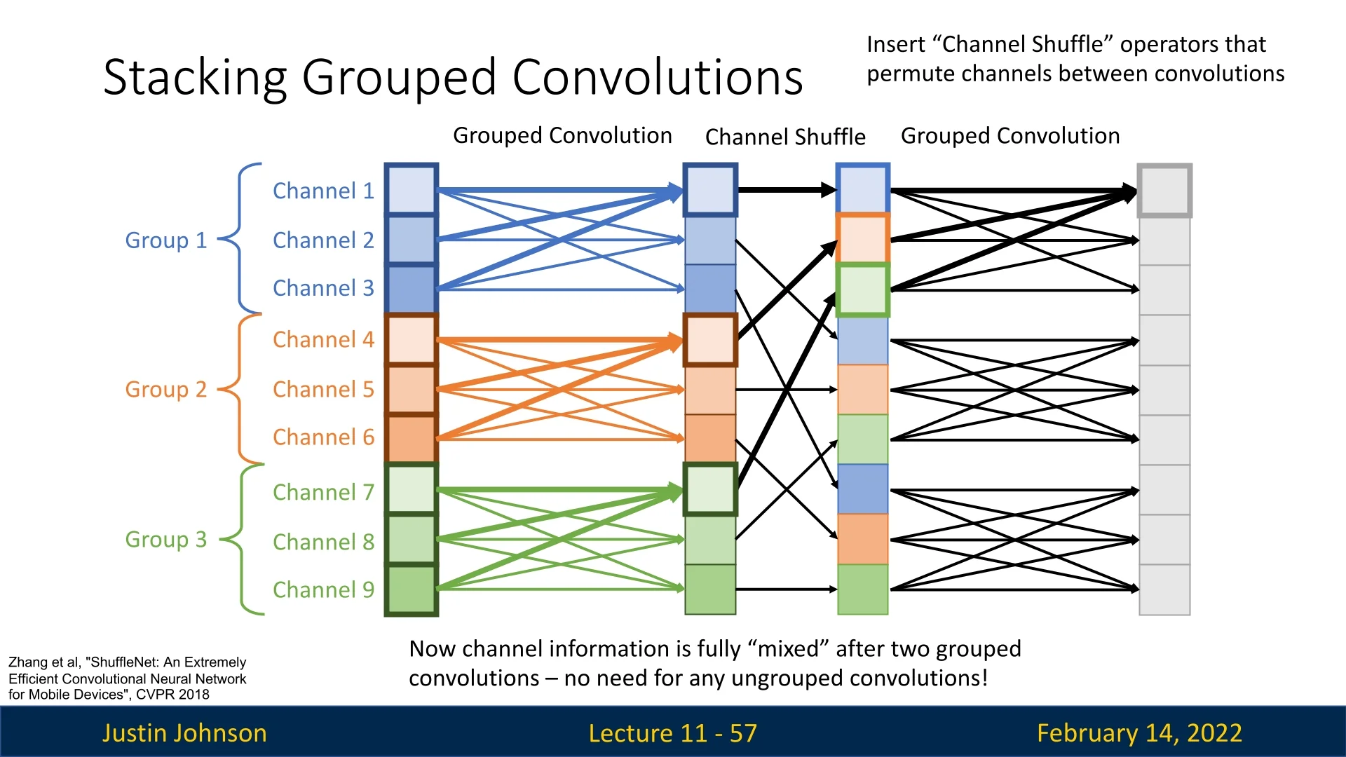
Solution: ShuffleNet [801]. ShuffleNet introduces the channel shuffle operation, which explicitly re-mixes channels across groups between successive grouped convolutions. The pattern is: \[ \mbox{grouped conv} \;\rightarrow \; \mbox{channel shuffle} \;\rightarrow \; \mbox{grouped conv}. \] After shuffling, each output group in the next layer receives channels originating from multiple input groups, restoring cross-group interaction while preserving the efficiency gains of grouped convolutions.
How the Channel Shuffle Works Consider a feature map \(X \in \mathbb {R}^{N \times C \times H \times W}\) (batch size \(N\), channels \(C\), height \(H\), width \(W\)) processed by a grouped convolution with \(g\) groups. The channels are conceptually partitioned into \(g\) groups of size \(C_g = C/g\) each. The channel shuffle is a fixed permutation of the channel dimension, implemented in three simple tensor operations:
- 1.
- Reshape: View the channel dimension as \((g, C_g)\): \[ X \in \mathbb {R}^{N \times C \times H \times W} \;\longrightarrow \; X' \in \mathbb {R}^{N \times g \times C_g \times H \times W}. \] Each of the \(g\) entries in the second dimension corresponds to one group.
- 2.
- Transpose (swap groups and within-group channels): \[ X' \in \mathbb {R}^{N \times g \times C_g \times H \times W} \;\longrightarrow \; X'' \in \mathbb {R}^{N \times C_g \times g \times H \times W}. \] This interleaves the channels so that positions that were previously in the same group are now spread across different groups.
- 3.
- Reshape back: \[ X'' \in \mathbb {R}^{N \times C_g \times g \times H \times W} \;\longrightarrow \; \tilde {X} \in \mathbb {R}^{N \times C \times H \times W}, \] where the channels of \(\tilde {X}\) are now a shuffled version of the original \(X\).
Intuitively, if you imagine dealing channels into \(g\) piles (groups), the shuffle operation re-deals them so that each new pile contains cards (channels) drawn from all the previous piles. When the next grouped convolution splits channels into \(g\) groups again, each group now contains information coming from all previous groups.
Differentiability of Channel Shuffle The channel shuffle is a purely indexing operation: it reorders channels but does not change their values. Mathematically, it corresponds to multiplying by a fixed permutation matrix along the channel dimension. Such a permutation is:
- Linear and invertible: no information is lost.
- Orthogonal: the inverse permutation simply reorders channels back.
During backpropagation, the gradient with respect to the input is obtained by applying the inverse permutation to the gradient with respect to the output. In practice, frameworks implement this as the same sequence of reshape/transpose operations in reverse order. Hence, the channel shuffle is fully differentiable and adds negligible computational overhead (no extra parameters, no multiplications), making it perfectly suitable for end-to-end training.
The ShuffleNet Unit
Motivation. In many lightweight CNNs (e.g., MobileNetV1), depthwise separable convolutions reduce the cost of spatial filtering, but the \(1\times 1\) pointwise convolutions remain expensive because they operate on all channels. ShuffleNet reduces this cost by:
- Applying grouped \(1\times 1\) convolutions to lower the FLOPs.
- Inserting a channel shuffle operation to avoid the isolation of channel groups.
- Grouped \(1\times 1\) Convolution: In contrast to ResNeXt (which typically groups only \(3\times 3\) convolutions), ShuffleNet also applies grouping to the \(1\times 1\) layers. Since pointwise convolutions often dominate the computation, grouping here yields substantial savings.
- Channel Shuffle Operation: Grouped convolutions alone process disjoint subsets of channels. By placing a channel shuffle between two grouped convolutions, ShuffleNet ensures that each group in the second convolution receives channels originating from multiple groups of the first, restoring effective cross-channel mixing.
Structure of a ShuffleNet Unit A standard ShuffleNet unit with stride \(1\) (Figure 11.22b) consists of:
- 1.
- A \(1\times 1\) grouped convolution (pointwise GConv), followed by batch normalization and a nonlinearity (e.g., ReLU).
- 2.
- A channel shuffle operation to re-mix channel groups.
- 3.
- A \(3\times 3\) depthwise convolution (DWConv) with stride 1, capturing spatial information at low cost, followed by batch normalization.
- 4.
- A second \(1\times 1\) grouped convolution to restore the channel dimension, followed by batch normalization.
- 5.
- A residual connection that adds the block input to the transformed output.
- 6.
- A final ReLU applied after the residual addition.
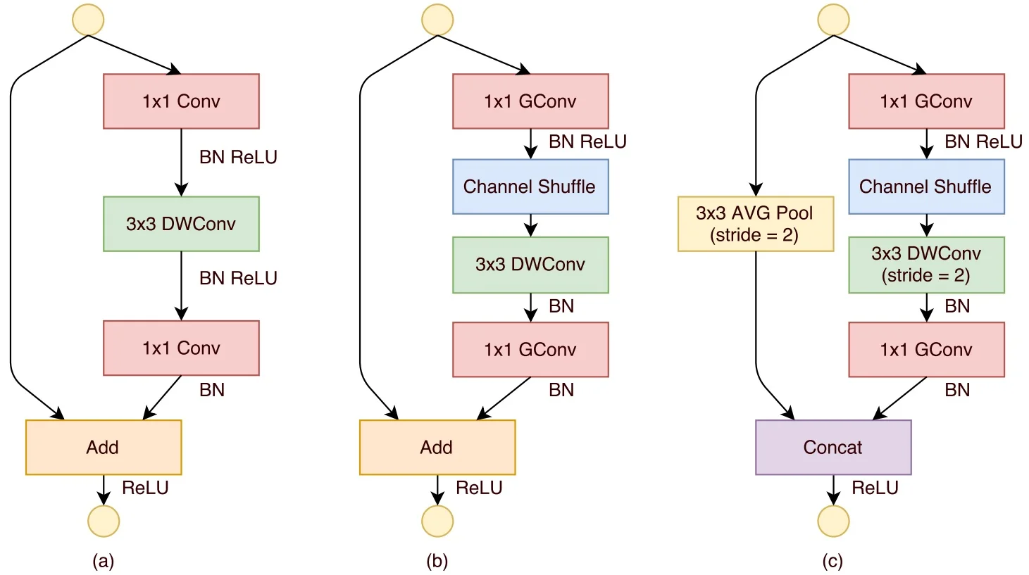
Stride-2 Modification When downsampling with stride \(2\) (Figure 11.22c), two modifications are introduced:
- The main branch uses a \(3\times 3\) depthwise convolution with stride \(2\) to reduce spatial resolution.
- The shortcut branch applies a \(3\times 3\) average pooling with stride \(2\) to match the main branch’s spatial dimensions.
- Instead of element-wise addition, the outputs of the main and shortcut branches are concatenated along the channel dimension. This preserves all features from both branches and increases the total number of channels, enhancing representational capacity.
ShuffleNet Architecture
The full ShuffleNet architecture is built by stacking ShuffleNet units into stages, similar to ResNet. Each stage operates at a fixed spatial resolution; the first unit in a stage downsamples and increases channels, while subsequent units keep the resolution constant.
- The first ShuffleNet unit in each stage performs downsampling with stride \(2\), reducing \(H\) and \(W\) while increasing the number of channels.
- Subsequent ShuffleNet units in the same stage use stride \(1\) to preserve spatial dimensions.
- At the beginning of each new stage, the number of output channels is doubled to compensate for reduced spatial resolution and maintain expressiveness.
- Within a ShuffleNet unit, the number of bottleneck channels is typically set to \(\frac {1}{4}\) of the block’s output channels, mirroring the bottleneck design in ResNet.
Scaling Factor Like other efficient models, ShuffleNet uses a width multiplier \(s\) to scale channel counts: \[ \mbox{ShuffleNet }s\times : \quad \#\mbox{Channels} = s \times \#\mbox{Channels in ShuffleNet }1\times . \] Increasing \(s\) increases model capacity and FLOPs (roughly by \(s^2\)), allowing practitioners to trade accuracy for compute depending on hardware constraints.
- Grouped \(1\times 1\) Convolutions reduce the cost of the most expensive layers.
- Channel Shuffle restores cross-group communication that would otherwise be lost with grouping.
- Stage-wise scaling (doubling channels when halving spatial size) balances efficiency and representational power across depth.
Overall, ShuffleNet provides an efficient alternative to MobileNet-type designs, showing how careful use of grouping and channel shuffling can reduce computation while preserving rich inter-channel mixing.
Computational Efficiency of ShuffleNet
To quantify ShuffleNet’s efficiency, consider a bottleneck block operating on an input feature map of spatial size \(H \times W\), with \(C\) input channels and \(m\) bottleneck channels. Let \(g\) denote the number of groups.
The approximate FLOPs for different bottleneck designs are:
- ResNet bottleneck block: \(H W \big (2 C m + 9 m^2\big )\) FLOPs.
- ResNeXt block: \(H W \big (2 C m + 9 m^2 / g\big )\) FLOPs (grouped \(3\times 3\) convolution).
- ShuffleNet block: \(H W \big (2 C m / g + 9 m\big )\) FLOPs (grouped \(1\times 1\), depthwise \(3\times 3\)).
Compared to ResNet and ResNeXt, ShuffleNet:
- reduces the cost of both \(1\times 1\) convolutions by a factor of \(g\), and
- replaces the dense \(3\times 3\) convolution (\(\mathcal {O}(m^2)\)) with a depthwise one (\(\mathcal {O}(m)\)).
This yields a substantial reduction in theoretical compute while maintaining good representational power via channel shuffle.
Inference Speed and Practical Performance
Theoretical FLOPs are only a proxy for real-world efficiency; memory access patterns and hardware characteristics matter as well. On ARM-based mobile processors, the ShuffleNet paper reports:
- A 4\(\times \) reduction in theoretical FLOPs compared to certain baselines translates into roughly a 2.6\(\times \) speedup in measured inference time.
- A group count of \(g = 3\) offers the best trade-off between accuracy and speed. Larger \(g\) (e.g., \(4\) or \(8\)) can slightly improve accuracy, but the extra overhead of more fragmented memory access and shuffling tends to hurt latency.
- The ShuffleNet \(0.5\times \) model achieves about a 13\(\times \) speedup over AlexNet in practice while maintaining comparable accuracy, despite a theoretical speedup of around \(18\times \).
These results highlight two key lessons:
- Channel shuffling makes grouped convolutions practically usable by restoring cross-channel mixing.
- Efficient architectures must be evaluated with both FLOPs and actual hardware performance in mind, especially for edge and mobile deployments.
Performance Comparison: ShuffleNet vs. MobileNet
To appreciate the practical impact of channel shuffling and grouped \(1\times 1\) convolutions, it is useful to compare ShuffleNet directly with MobileNetV1 at a similar computational budget on ImageNet.
| Model | Top-1 Accuracy (%) | Multi-Adds (M) | Parameters (M) |
|---|---|---|---|
| MobileNetV1 1.0\(\times \) (224) | 70.6 | 569 | 4.2 |
| ShuffleNet 1.0\(\times \) (g=3) | 71.7 | 524 | 5.0 |
In this regime, ShuffleNet gains accuracy per FLOP by (i) replacing dense \(1\times 1\) convolutions with grouped ones and (ii) restoring cross-channel interaction via channel shuffle. MobileNetV1 relies on depthwise separable convolutions but still uses dense \(1\times 1\) mixing; ShuffleNet shows that, with a carefully designed permutation (the shuffle), even the pointwise layers can be aggressively factorized without sacrificing, and in fact slightly improving, accuracy.
Beyond ShuffleNet: Evolution of Efficient CNN Architectures
ShuffleNet is part of a broader line of work on efficient CNNs for mobile and embedded devices. Its core ideas—cheap spatial filtering (depthwise conv), structured sparsity (grouped \(1\times 1\) conv), and explicit channel mixing (shuffle)—influenced how later architectures think about trading off compute, memory, and accuracy.
Subsequent models extend these principles in different directions:
- MobileNetV2 introduces inverted residuals with linear bottlenecks, using depthwise convolutions inside narrow–wide–narrow blocks to reduce computation while preserving information in low-dimensional spaces.
- MobileNetV3 combines MobileNetV2-style blocks with neural architecture search (NAS) and lightweight attention (SE blocks), explicitly optimizing for mobile hardware latency rather than FLOPs alone.
- RegNet focuses on designing regular, scalable CNN families whose width and depth follow simple rules; under similar FLOP budgets, RegNet models have been reported to match EfficientNet-level accuracy while requiring up to \(\sim \)5\(\times \) fewer training iterations.
We will revisit these architectures in later chapters. For now, ShuffleNet serves as a key example of how seemingly simple operations—grouped convolutions plus a differentiable channel permutation—can dramatically improve the efficiency of convolutional networks while maintaining strong accuracy on large-scale benchmarks.
11.5.3 MobileNetV2: Inverted Bottleneck and Linear Residual
Motivation: When to Apply Non-Linearity?
MobileNetV2 [562] builds upon MobileNetV1’s depthwise-separable design but
further refines how and where non-linear activations are applied. The
key insight is that applying a non-linearity such as ReLU at the wrong
stage—particularly after reducing the channel dimension—can irreversibly
discard useful information.
Instead, MobileNetV2 proposes:
“Apply non-linearity in the expanded, high-dimensional space before projecting back linearly to a lower-dimensional representation.”
This ensures that the most expressive transformations occur in a rich, high-dimensional space, and the final projection back to a lower-dimensional space does not suffer from information loss due to ReLU-induced zeroing-out of channels.
Understanding Feature Representations and Manifolds A convolutional layer with an output shape of \( h \times w \times d \) can be interpreted as a grid of \( h \times w \) spatial locations, where each location contains a \( d \)-dimensional feature vector. Although this representation is formally \( d \)-dimensional, empirical evidence suggests that the manifold of interest—the meaningful variation within these activations—often resides in a much lower-dimensional subset. In other words, not all \( d \) dimensions contain independently useful information; instead, they are highly correlated, meaning they effectively form a low-dimensional structure within the high-dimensional activation space.
ReLU and Information Collapse Applying ReLU in a low-dimensional subspace can lead to an irreversible loss of information. To illustrate this, consider the following experiment:
- A 2D spiral is embedded into an \(n\)-dimensional space using a random matrix transformation \(T\).
- A ReLU activation is applied in this \(n\)-dimensional space.
- The transformed data is then projected back to 2D using \(T^{-1}\).
- When \(n\) is small (e.g., \(n=2\) or \(n=3\)), ReLU distorts or collapses the manifold, as important information is lost when negative values are clamped to zero.
- When \(n\) is large (\(n \geq 15\)), the manifold remains well-preserved, as the high-dimensional space allows the ReLU transformation to retain sufficient structure.
This experiment highlights a key principle: non-linearity should be applied in a sufficiently high-dimensional space to avoid information collapse. This directly motivates the MobileNetV2 design, which introduces an inverted residual block.
The MobileNetV2 Block: Inverted Residuals and Linear Bottleneck
Why “Inverted Residual”?
Traditional residual blocks, such as those in ResNet, transform wide feature
representations into a narrow bottleneck before expanding back. MobileNetV2
inverts this pattern: it starts with a narrow representation, expands it using
a pointwise convolution, applies a depthwise convolution, then projects it
back to a narrow representation. This is why it is called an inverted
residual.
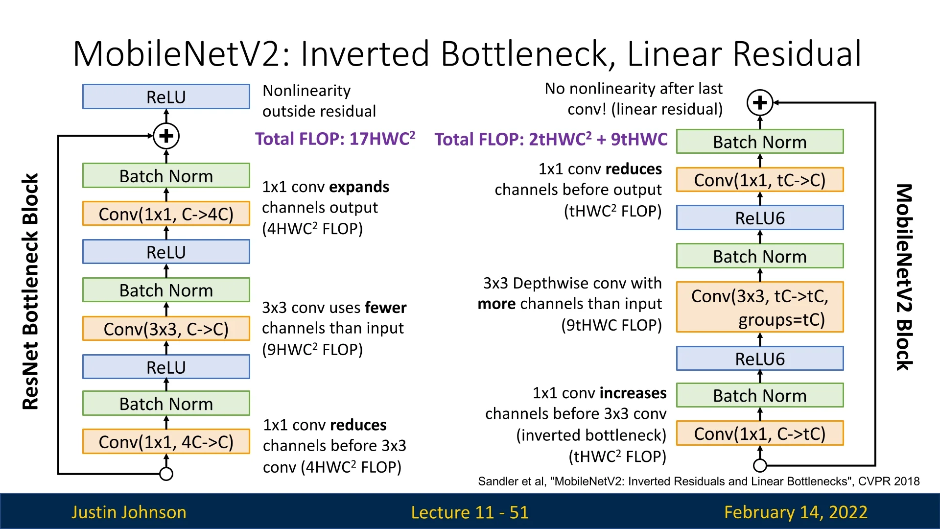
Detailed Block Architecture Each MobileNetV2 block consists of:
- 1.
- Expansion (\(1\times 1\) conv + ReLU6): Increases the channel dimension by an expansion factor \(t\) (typically \(t=6\)), allowing non-linearity to operate in a richer space.
- 2.
- Depthwise Conv (\(3\times 3\) + ReLU6): Efficiently captures spatial features with minimal cross-channel computation.
- 3.
- Projection (\(1\times 1\) conv, no ReLU): Reduces back to the original (narrow) dimension. This step is linear to prevent information loss due to non-linearity.
- 4.
- Residual Connection: If the input and output shapes match (same spatial size and number of channels), a skip connection adds the input to the output.
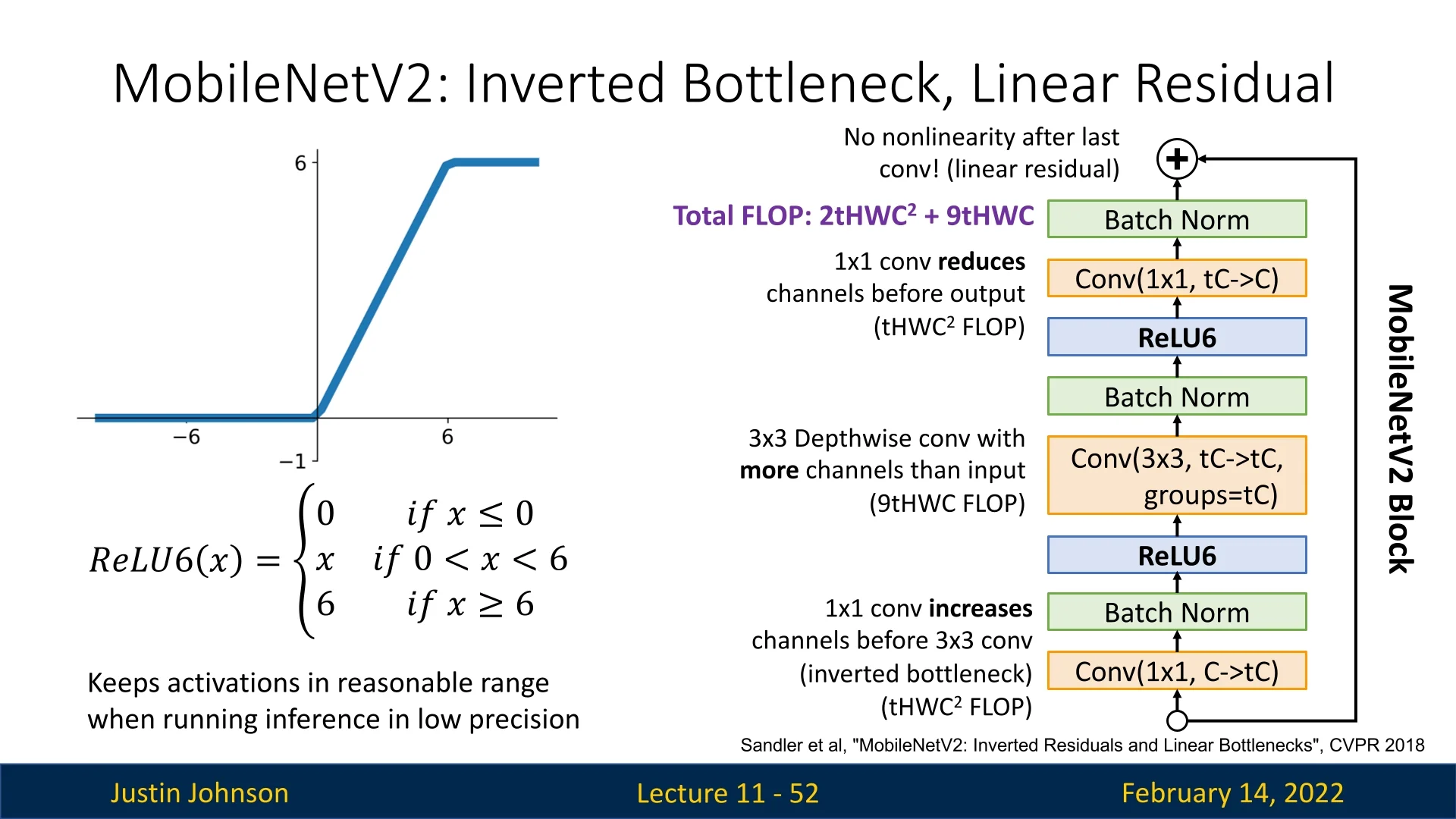
ReLU6 and Its Role in Low-Precision Inference
Definition and Motivation
MobileNetV2 employs ReLU6 instead of standard ReLU, defined as: \[ \mathrm {ReLU6}(x)\;=\;\min \bigl (\max (0,\,x),\,6\bigr ). \] This
choice was primarily motivated by:
- Activation Range Constraint: Since ReLU6 clamps values between 0 and 6, it prevents extremely large activations that could dominate later layers, improving numerical stability.
- Fixed-Point Quantization Stability: In 8-bit integer arithmetic, numbers are typically represented with limited dynamic range. By keeping activations within a well-bounded range, ReLU6 reduces precision loss when mapping from floating-point to integer representation.
Practical Observations and Alternatives Later research [316] found that:
- ReLU6 does not always improve quantization. While it was originally intended to make 8-bit inference more robust, in practice, most modern quantization techniques can handle ReLU just as well.
- ReLU can sometimes outperform ReLU6. In particular, in cases where higher activation values play a role in separating decision boundaries, the strict upper bound of ReLU6 can be detrimental.
As a result, later architectures such as MobileNetV3 have moved back to using standard ReLU.
Why is the Inverted Block Fitting to Efficient Networks?
At first glance, temporarily expanding the channel dimension before processing and then narrowing it again seems to introduce additional computational cost compared to a straightforward bottleneck or MobileNetV1’s depthwise-separable design. However, MobileNetV2 often achieves higher accuracy at similar or only slightly higher FLOPs due to the following key factors:
1. Depthwise Convolutions Maintain Low Computational Cost As in MobileNetV1, each \(3\times 3\) depthwise convolution operates on each channel separately, reducing computational complexity from: \[ \mathcal {O}(k^2 \cdot \mbox{height} \cdot \mbox{width} \cdot \mbox{channels_in} \times \mbox{channels_out}) \] to: \[ \mathcal {O}(k^2 \cdot \mbox{height} \cdot \mbox{width} \cdot \mbox{channels_in}) \] This ensures that most of the FLOPs in each block remain low despite the temporary expansion of channels.
2. Moderate Expansion Factor \((t)\) Balances Efficiency The expansion factor \(t\) determines how much the channel dimension increases inside the block. In practice, \(t=6\) is commonly used, striking a balance between expressivity and computational efficiency. This expansion allows non-linear transformations (via ReLU) to operate in a higher-dimensional space, reducing the risk of losing critical channels while ensuring that the final projection does not incur excessive overhead.
3. Comparison to MobileNetV1 The computational cost of a single block in each architecture is:
- MobileNetV1: \(\mathcal {O}((9C + C^2)HW)\)
- MobileNetV2: \(\mathcal {O}((9tC + 2tC^2)HW)\) per block, due to channel expansion.
Although MobileNetV2 appears to introduce additional cost, the overall network remains efficient because:
- MobileNetV2 has fewer layers than MobileNetV1. While the original MobileNetV1 consists of 28 layers, MobileNetV2 reduces this number to 17.
- MobileNetV2 has wider representations per layer. Since each block expands channels internally, fewer layers are needed to reach a comparable expressive power.
- The cost gap between the two architectures decreases as the channel count increases. Specifically, for large \(C\), the cost of MobileNetV1 (which has \(\mathcal {O}(C^2)\) terms) becomes comparable to the cost of MobileNetV2 with moderate expansion (\(t=6\)).
Empirically, MobileNetV2 achieves higher accuracy per FLOP compared to MobileNetV1, making the trade-off worthwhile.
4. Comparison to ResNet Bottleneck Blocks While MobileNetV2 is inspired by ResNet’s bottleneck design, the computational costs differ:
- ResNet bottleneck: \(\mathcal {O}(17HWC^2)\)
- MobileNetV2 bottleneck: \(\mathcal {O}(2tHWC^2 + 9tHWC)\)
For moderate values of \(t\), e.g., \(t=6\), we have: \[ \mbox{MobileNetV2 is more efficient than ResNet if: } 54HWC < 5HWC^2 \] At high channel counts, the computational gap reduces significantly. In some cases, MobileNetV2 blocks can even be more efficient than ResNet bottlenecks.
5. Linear Bottleneck Preserves Subtle Features Unlike traditional residual connections, MobileNetV2 omits ReLU in the final projection layer. This ensures that small but useful activations are not lost when projecting back to the lower-dimensional space. This is particularly important in low-dimensional feature spaces where aggressive non-linearity can collapse valuable information.
Summary Although the MobileNetV2 block seems computationally heavier than MobileNetV1 on a per-block basis, the overall network-level architecture is more efficient because:
- It requires fewer total layers.
- Fewer downsampling stages are used in deeper layers.
- It achieves significantly better accuracy at a similar FLOP budget.
MobileNetV2 Architecture and Performance
Network Structure MobileNetV2 consists of:
| Input | Operator | #Repeats | Expansion | Output Channels |
|---|---|---|---|---|
| \(224^2 \times 3\) | \(3\times 3\) Conv (stride 2) | 1 | – | 32 |
| \(112^2 \times 32\) | Inverted Residual Block | 1 | 1 | 16 |
| \(112^2 \times 16\) | Inverted Residual Block | 2 | 6 | 24 |
| \(56^2 \times 24\) | Inverted Residual Block | 3 | 6 | 32 |
| \(28^2 \times 32\) | Inverted Residual Block | 4 | 6 | 64 |
| \(14^2 \times 64\) | Inverted Residual Block | 3 | 6 | 96 |
| \(14^2 \times 96\) | Inverted Residual Block | 3 | 6 | 160 |
| \(7^2 \times 160\) | Inverted Residual Block | 1 | 6 | 320 |
| \(7^2 \times 320\) | \(1\times 1\) Conv | 1 | – | 1280 |
Comparison to MobileNetV1, ShuffleNet, and NASNet
Efficiency and Accuracy Trade-offs
MobileNetV2 refines MobileNetV1’s depthwise-separable design and
introduces inverted residuals and linear bottlenecks, leading to
better efficiency-accuracy trade-offs. Compared to alternative lightweight
architectures, it strikes a balance between computational cost and real-world
deployability.
| Network | Top-1 Acc. (%) | Params (M) | MAdds (M) | CPU Time (ms) |
|---|---|---|---|---|
| MobileNetV1 | 70.6 | 4.2M | 575M | 113ms |
| ShuffleNet (1.5×) | 71.5 | 3.4M | 292M | - |
| ShuffleNet (2×) | 73.7 | 5.4M | 524M | - |
| NASNet-A | 74.0 | 5.3M | 564M | 183ms |
| MobileNetV2 | 72.0 | 3.4M | 300M | 75ms |
| MobileNetV2 (1.4×) | 74.7 | 6.9M | 585M | 143ms |
Key Observations:
- MobileNetV2 vs. MobileNetV1: MobileNetV2 achieves 1.4% higher accuracy while reducing Multiply-Adds by nearly 50%. This efficiency gain comes from inverted residuals and linear bottlenecks, which prevent feature collapse in low-dimensional spaces and allow to reduce the number of layers significantly while retaining representational power.
-
MobileNetV2 vs. ShuffleNet: ShuffleNet (2×) achieves a slightly higher 73.7% accuracy but at a higher computational cost (524M Multiply-Adds vs. 300M for MobileNetV2). MobileNetV2 remains more widely used due to better hardware support for its depthwise operations.
- MobileNetV2 vs. NASNet-A: NASNet-A, designed via Neural Architecture Search (NAS), achieves the highest accuracy (74.0%) but is significantly slower (183ms inference time vs. 75ms for MobileNetV2).
Motivation for NAS and MobileNetV3
While MobileNetV2 optimizes manual architecture design, NASNet-A highlights
the potential of automated architecture search to find even better
efficiency-accuracy trade-offs. However, its high computational cost motivates
MobileNetV3, which builds on MobileNetV2 while incorporating NAS
techniques to optimize block structures, activation functions, and expansion
ratios for real-world deployment.
The next section explores NAS and MobileNetV3, bridging the gap between handcrafted and automatically optimized architectures.
11.5.4 Neural Architecture Search (NAS) and MobileNetV3
Neural Architecture Search (NAS): Automating Architecture
Design
Designing neural network architectures is a challenging and time-consuming task.
Neural Architecture Search (NAS) [831, 832] aims to automate this process by using a
controller network that learns to generate optimal architectures through
reinforcement learning.
How NAS Works? Policy Gradient Optimization
Neural Architecture Search (NAS) uses a controller network to generate candidate architectures, which are then evaluated to improve the search strategy. However, the challenge is that architectural search is non-differentiable. It is not possible to directly compute gradients for better architectures. Instead, NAS relies on policy gradient optimization, a reinforcement learning (RL) technique, to update the controller.
What is a Policy Gradient? In reinforcement learning, an agent interacts with an environment and takes actions based on a learned policy to maximize a reward. The policy is typically parameterized by a neural network, and a policy gradient method updates these parameters by computing gradients with respect to expected future rewards.
For NAS:
- The controller network acts as the RL agent, outputting architectural decisions (e.g., filter sizes, number of layers).
- The child networks sampled from the controller act as the environment; they are trained and evaluated on a dataset.
- The reward function is defined based on the validation accuracy of the sampled child networks.
Updating the Controller Using Policy Gradients NAS applies the REINFORCE algorithm [716] to update the controller network: \begin {equation} \nabla J(\theta ) = \mathbb {E} \left [ \sum _{t=1}^{T} \nabla _{\theta } \log p(a_t | \theta ) R \right ], \end {equation} where:
- \( \theta \) are the controller’s parameters.
- \( a_t \) represents architectural choices (e.g., layer types, kernel sizes).
- \( R \) is the reward (child network validation accuracy).
Intuitively, this means:
- 1.
- Sample an architecture.
- 2.
- Train it and measure its accuracy.
- 3.
- Update the controller to reinforce architectural decisions that led to better accuracy.
Over time, NAS converges to high-performing architectures.
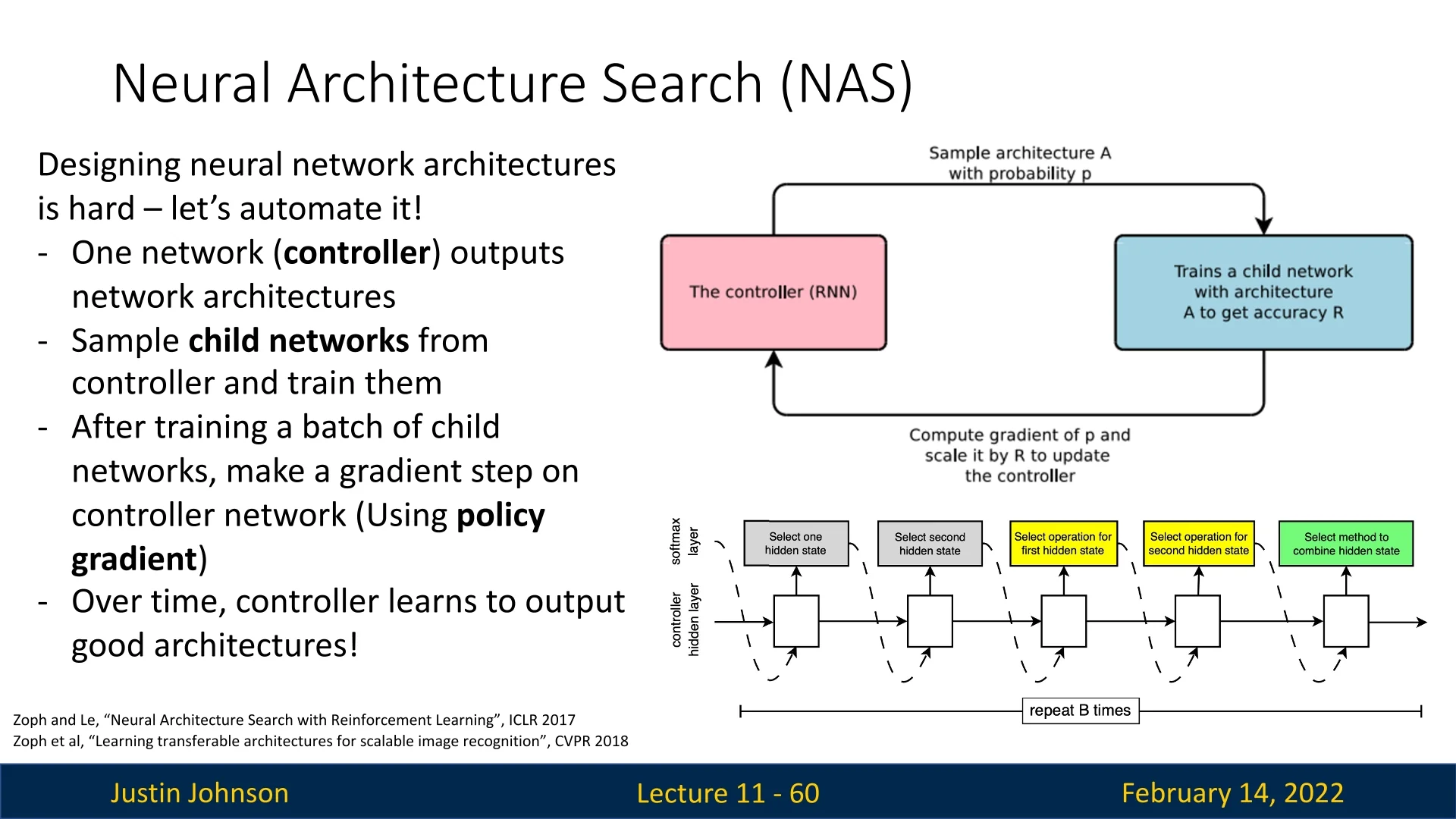
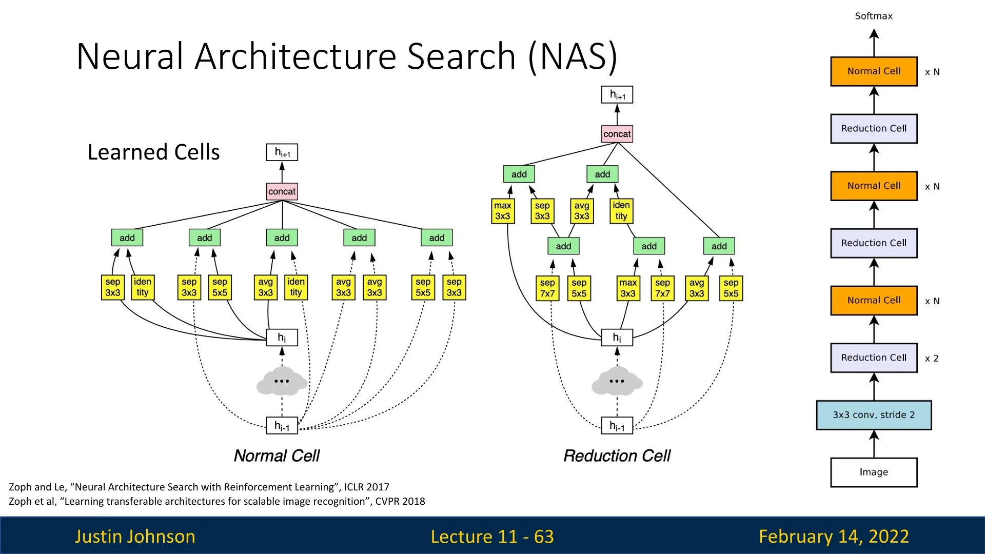
Searching for Reusable Block Designs Rather than searching for an entire architecture from scratch, NAS focuses on identifying efficient reusable blocks, which can be stacked to construct a full network. The search space consists of various operations, including:
- Identity
- \(1\times 1\) convolution
- \(3\times 3\) convolution
- \(3\times 3\) dilated convolution
- \(1\times 7\) followed by \(7\times 1\) convolution
- \(1\times 3\) followed by \(3\times 1\) convolution
- \(3\times 3\), \(5\times 5\), or \(7\times 7\) depthwise-separable convolutions
- \(3\times 3\) average pooling
- \(3\times 3\), \(5\times 5\), or \(7\times 7\) max pooling
NAS identifies two primary block types:
- Normal Cell: Maintains the same spatial resolution.
- Reduction Cell: Reduces spatial resolution by a factor of \(2\).
These cells are then combined in a regular pattern to construct the final architecture.
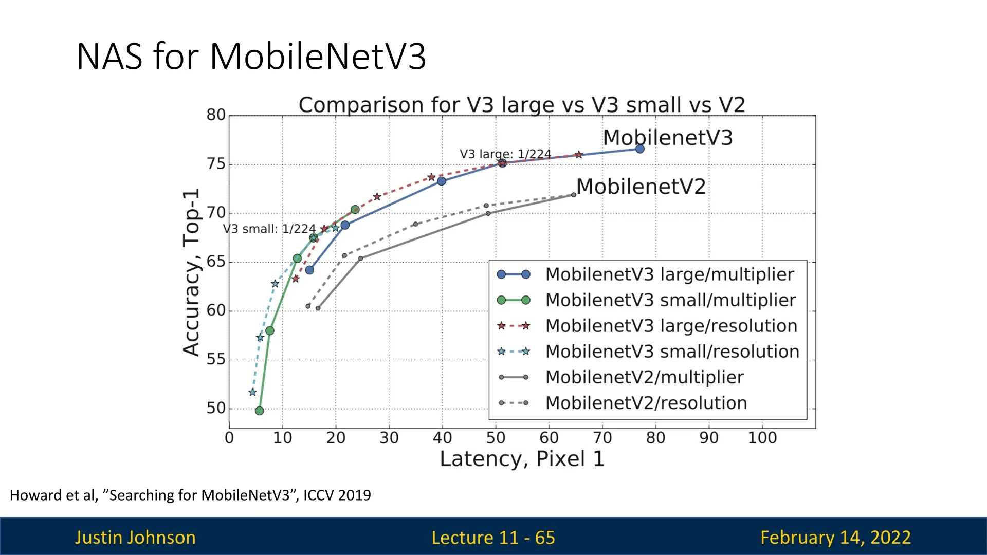
MobileNetV3: NAS-Optimized Mobile Network
Motivation and Evolution from MobileNetV2.
MobileNetV3 [240] builds upon MobileNetV2 by leveraging NAS to further
optimize key architectural choices. It incorporates:
- EfficientNet-style NAS search to refine block selection and expansion ratios.
- Swish-like activation function (h-swish) to improve non-linearity efficiency.
- Squeeze-and-Excitation (SE) modules in some layers to improve channel-wise attention.
- Smaller and optimized depthwise convolutions, reducing computational cost while maintaining expressiveness.
The MobileNetV3 Block Architecture and Refinements
MobileNetV3 [240] was developed using NAS, which optimized its block structure, activation functions, and efficiency improvements.
Structure of the MobileNetV3 Block The core MobileNetV3 block builds upon the MobileNetV2 inverted residual block but introduces:
- Squeeze-and-Excitation (SE) modules to enhance important features.
- h-swish activation instead of ReLU6 for better non-linearity.
- Smaller depthwise convolutions to reduce computation.
Differences from Previous MobileNet Blocks
- MobileNetV1 Used standard depthwise separable convolutions.
- MobileNetV2 Introduced the inverted residual block and linear bottlenecks.
- MobileNetV3 Enhances MobileNetV2 with NAS-optimized activation functions and attention mechanisms.
Why is MobileNetV3 More Efficient?
At first glance, MobileNetV3 may seem computationally more expensive than MobileNetV2 since it builds upon the same inverted residual block while introducing additional mechanisms like squeeze-and-excitation (SE). However, it is actually more efficient due to several optimizations discovered through NAS.
Key Optimizations That Improve Efficiency
- Neural Architecture Search (NAS) Optimization: NAS optimizes layer types, kernel sizes, and expansion ratios to minimize latency on real-world mobile hardware. Rather than using a fixed design like MobileNetV2, NAS learns the most efficient way to balance depthwise separable convolutions, SE blocks, and activation functions.
- Selective Use of SE Blocks: While SE blocks add computation, NAS only places them in layers where they provide the most accuracy gain per FLOP. MobileNetV2 did not use the channel-attention mechanism at all, whereas MobileNetV3 strategically incorporates SE only in certain depthwise layers, preventing unnecessary overhead.
- h-swish Activation: ReLU6 was initially introduced in MobileNetV2 for quantization robustness but has a hard threshold at 6, limiting its expressiveness. MobileNetV3 replaces it with h-swish, approximates the smoothness of Swish (more computationally efficient): \begin {equation} \mbox{h-swish}(x) = x \cdot \frac {\max (0, \min (x+3, 6))}{6}. \end {equation} This activation function improves accuracy and stability with little extra computational cost.
- Fewer Depthwise Layers, Higher Efficiency: NAS found that some depthwise convolutions in MobileNetV2 were redundant. By reducing the number of depthwise layers in specific parts of the network while slightly increasing the expansion ratio elsewhere, MobileNetV3 achieves a better accuracy-FLOP tradeoff.
- Better Parallelism and Memory Access Efficiency: MobileNetV3 is designed to maximize memory access efficiency (avoiding network fragmentation) and parallel execution on ARM-based chips.
Empirical Comparison of MobileNetV3 MobileNetV3 introduces architecture search and network-level optimizations that make it both faster and more accurate than its predecessors.
| Family | Variant | Top-1 Acc. (%) | MAdds (M) | Latency (ms) |
|---|---|---|---|---|
| MobileNetV1 [239] | 1.0 MobileNet-224 | 70.6 | 569 | 119 |
| MobileNetV2 [562] | 1.0 MobileNetV2-224 | 72.0 | 300 | 72 |
| MobileNetV3 [240] | Large 1.0 | 75.2 | 219 | 51 |
| MobileNetV3 [240] | Small 1.0 | 67.4 | 66 | 15.8 |
| MnasNet [622] | A1 (baseline) | 75.2 | 312 | 70 |
| ProxylessNAS [61] | GPU-targeted | 74.6 | 320 | 78 |
MobileNetV3-Large matches the accuracy of MnasNet-A1 while using 30% fewer multiply-add operations and achieving over 25% lower latency. Compared to MobileNetV2, it improves Top-1 accuracy by more than 3%, with a 27% reduction in computation and substantially lower inference time—making it an attractive choice for high-performance mobile inference.
The Computational Cost of NAS and Its Limitations
Despite its success in automating architecture search, Neural Architecture Search (NAS) is computationally expensive, making it impractical for many real-world applications.
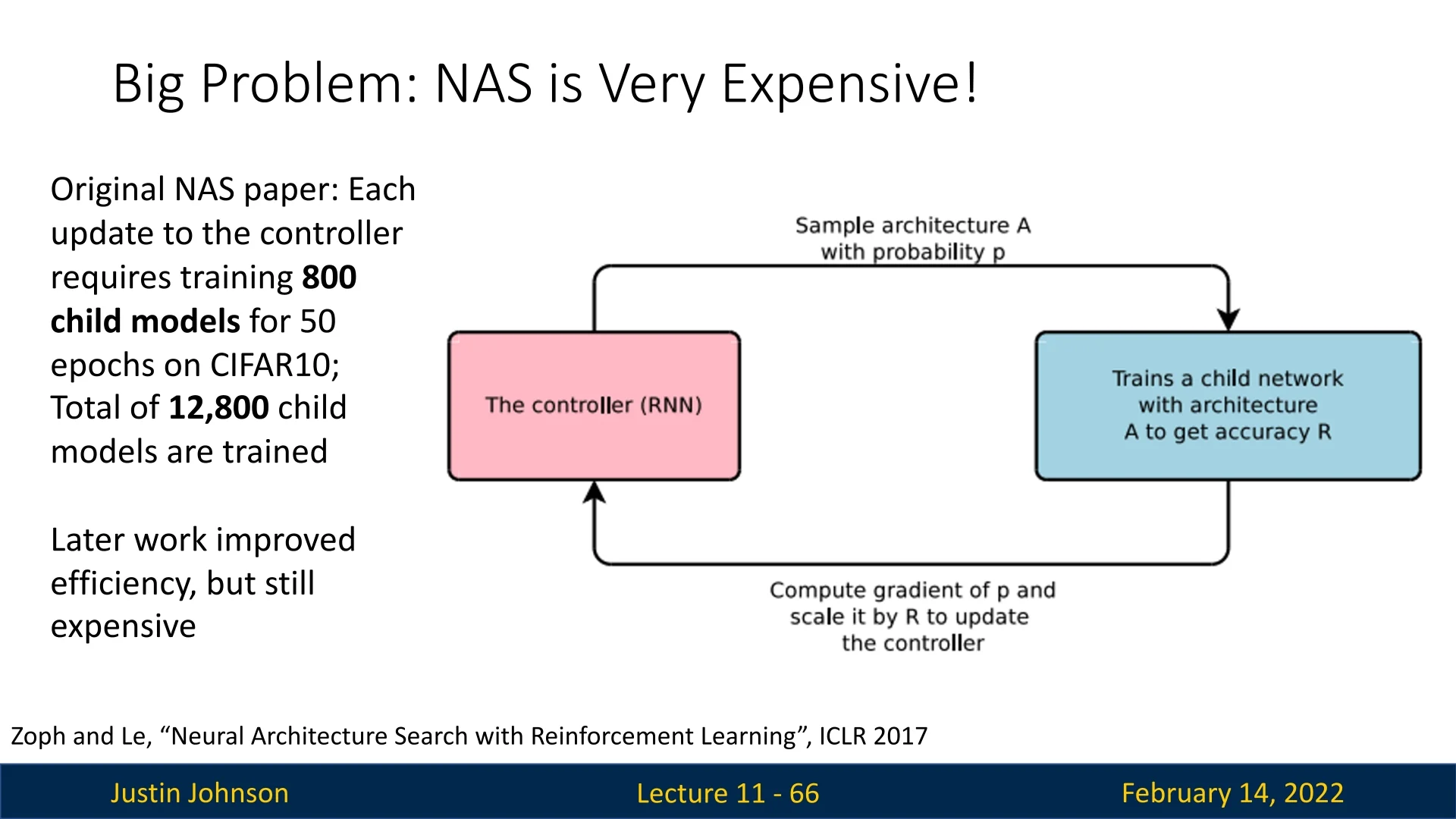
- Training Thousands of Models: NAS relies on evaluating a vast number of candidate architectures, requiring immense computational resources.
- Slow Policy Gradient Optimization: Unlike standard gradient-based training, NAS often uses reinforcement learning techniques, such as policy gradients, which require many optimization steps to converge.
- Fragmented and Inefficient Architectures: NAS-generated networks may be highly fragmented, reducing their parallel execution efficiency on modern hardware.
- High Parallelism is Often Inefficient: While NAS models aim to maximize hardware utilization, excessive fragmentation and complex layer dependencies can slow down inference.
While NAS has produced strong models like MobileNetV3, its computational cost remains a major bottleneck. This motivates alternative approaches that focus on efficiency without requiring exhaustive search.
ShuffleNetV2 and Practical Design Rules
Why ShuffleNetV2? Whereas ShuffleNetV1 focused on reducing theoretical FLOPs via group convolutions and channel shuffling, ShuffleNetV2 [420] reorients the goal toward real-world efficiency. This shift stems from a key observation: FLOPs are a poor predictor of actual inference time on mobile and embedded hardware. In practice, performance is often dominated by the memory access cost (MAC)—that is, the latency and bandwidth required to move data between memory and compute units, not the number of multiply–accumulate operations.
Because modern mobile SoCs (System-on-Chips) are highly parallel but memory-bound, factors like tensor fragmentation, channel imbalance, and excessive branching can bottleneck throughput. ShuffleNetV2 addresses these bottlenecks through four pragmatic design rules that align the network’s dataflow with hardware constraints, yielding smoother parallelism and lower latency.
Four Key Guidelines for Practical Efficiency The authors propose four guidelines—each derived from profiling real devices—to ensure that architectural efficiency translates into real speedups:
- 1.
- G1: Equal channel widths minimize memory access cost. Maintaining consistent channel dimensions across layers minimizes intermediate buffering and reindexing, reducing the number of cache misses and memory stalls.
- 2.
- G2: Excessive group convolutions raise memory access cost. While group convolutions reduce FLOPs, they fragment tensors into small sub-blocks. Each sub-block requires independent reads and writes, increasing data movement and synchronization overhead.
- 3.
- G3: Excessive network fragmentation hinders parallelism. Architectures that repeatedly split and merge feature maps (e.g., multi-path or highly branched designs) prevent hardware from exploiting full parallelism, since many cores must wait for partial results.
- 4.
- G4: Element-wise operations are non-negligible. Operations such as Add, ReLU, and channel shuffling have small FLOP counts but non-trivial memory and kernel-launch costs. Minimizing or fusing them improves latency.
From ShuffleNetV1 to ShuffleNetV2 ShuffleNetV1 achieved strong FLOP reductions but violated several of these principles in practice:
- The heavy use of grouped \(1\times 1\) convolutions (often with large \(g\)) increased MAC (violating G2).
- The frequent split–shuffle–concat sequences introduced fragmentation (violating G3).
ShuffleNetV2 remedies this with a streamlined design:
- It removes grouping from most \(1\times 1\) convolutions (reducing G2 overhead).
- It enforces uniform channel splits (satisfying G1) and applies only one shuffle after concatenation (reducing G4).
- It simplifies the data path into a near-linear flow with minimal branching (satisfying G3).
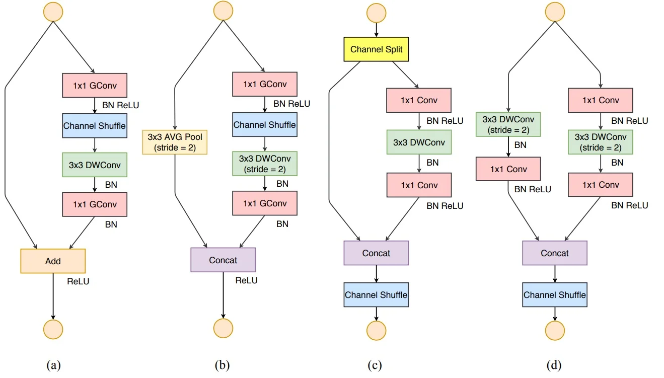
The ShuffleNetV2 Unit: Architecture and Intuition The new ShuffleNetV2 block (Figure 11.30c) is carefully structured to follow these principles:
- 1.
- Channel Split: The input tensor (with \(C\) channels) is evenly split into two halves (\(C/2\) each). One half forms a lightweight identity branch, and the other half forms a processing branch.
- 2.
- Processing Branch: The active half passes through a standard (non-grouped) \(1\times 1\) convolution, followed by a \(3\times 3\) depthwise convolution (DWConv) and another \(1\times 1\) convolution. All layers maintain constant channel width (\(C/2\)), adhering to G1. Removing group convolutions and keeping uniform channel widths directly lowers MAC and fragmentation.
- 3.
- Concatenation and Shuffle: The processed output and the untouched identity branch are concatenated, restoring the total channel count to \(C\). A single channel shuffle then mixes the two halves, ensuring that subsequent blocks receive blended information without needing multiple permutations.
- 4.
- Stride-2 Variant: For downsampling (Figure 11.30d), both branches are active. The main branch applies depthwise convolution with stride 2, and the shortcut branch uses a parallel \(3\times 3\) depthwise convolution followed by concatenation. This doubles channel count while halving spatial resolution, avoiding extra addition or pooling operations.
This design nearly eliminates redundant memory movement while retaining strong feature interaction—demonstrating that well-structured simplicity can outperform complex multi-branch patterns.
Performance vs. MobileNetV3 Although ShuffleNetV2 achieves excellent hardware efficiency and latency, it does not always surpass MobileNetV3 in accuracy at equivalent FLOP budgets. Key reasons include:
- Inverted Bottlenecks (MobileNetV3): MobileNetV3 expands and compresses channels asymmetrically, seemingly violating G1’s uniformity rule. However, its NAS-optimized expansions and fusions exploit hardware more effectively, offsetting theoretical inefficiencies.
- Neural Architecture Search (NAS): While ShuffleNetV2 follows fixed rules, MobileNetV3 uses NAS to explore exceptions—sometimes deliberately introducing non-uniform widths or SE-blocks that slightly increase MAC but improve accuracy and speed once fused.
- Real-world Latency: On mobile CPUs and NPUs, MobileNetV3’s fused inverted residual blocks often run 10–15% faster than ShuffleNetV2, thanks to reduced kernel launches and optimized operator fusion.
Despite this, ShuffleNetV2’s four design rules remain highly influential. They codified practical guidelines for mapping convolutional networks efficiently onto real hardware—guidelines that informed both NAS search spaces and the design of later lightweight models such as MobileNetV3 and EfficientNet-Lite.
The Need for Model Scaling and EfficientNets
Beyond Hand-Designed and NAS-Optimized Models While manually designed architectures (e.g., ShuffleNetV2) and NAS-optimized networks (e.g., MobileNetV3) have driven major advancements in efficiency, there is still room for improvement. The search for better trade-offs between accuracy and computational cost has led researchers to a fundamental question:
Instead of searching for entirely new architectures, can we systematically scale existing models to achieve optimal efficiency?
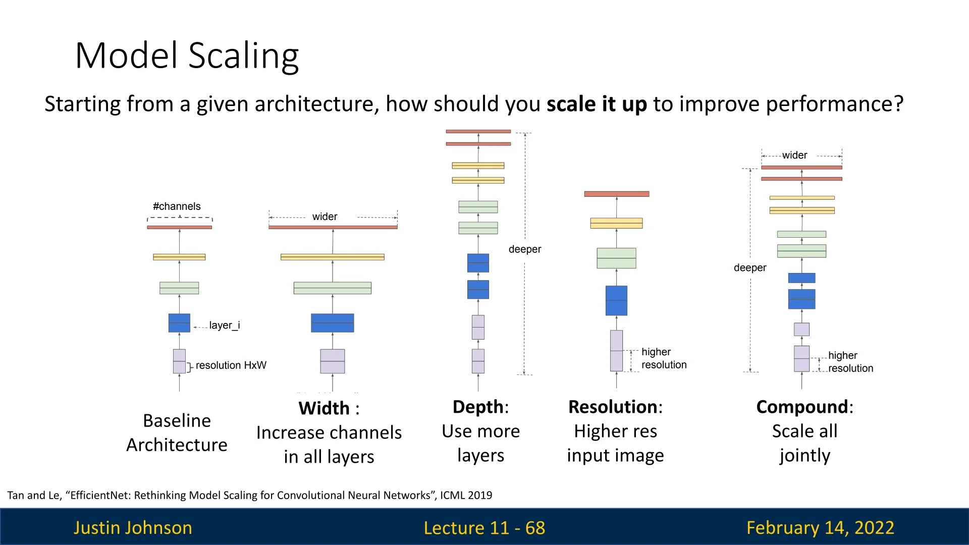
Rather than focusing solely on designing better building blocks or running expensive NAS procedures, an alternative approach emerged: scaling existing models in a structured manner. Scaling a model can involve increasing:
- Depth: Adding more layers to increase representational power.
- Width: Expanding the number of channels per layer.
- Resolution: Using larger input images to capture finer details.
However, scaling any single dimension in isolation often leads to suboptimal results. Increasing depth alone may result in diminishing returns, while scaling width or resolution independently can make models inefficient. Instead, we need a principled way to scale these three dimensions together.
Introducing EfficientNet To address this challenge, EfficientNet [621] was proposed, leveraging a compound scaling approach that jointly optimizes depth, width, and resolution in a balanced way. By using a carefully tuned scaling coefficient, EfficientNet ensures that all three dimensions grow in harmony, yielding models that maximize accuracy while minimizing computational cost.
11.6 EfficientNet Compound Model Scaling
11.6.1 How Should We Scale a Model
Given a well-designed baseline architecture, a fundamental question arises:
How should we scale it up to improve performance while maintaining efficiency?
Common approaches to scaling include:
- Width Scaling: Increasing the number of channels per layer to capture more fine-grained features.
- Depth Scaling: Adding more layers to allow deeper feature extraction and better generalization.
- Resolution Scaling: Using higher-resolution images to enhance spatial feature learning.
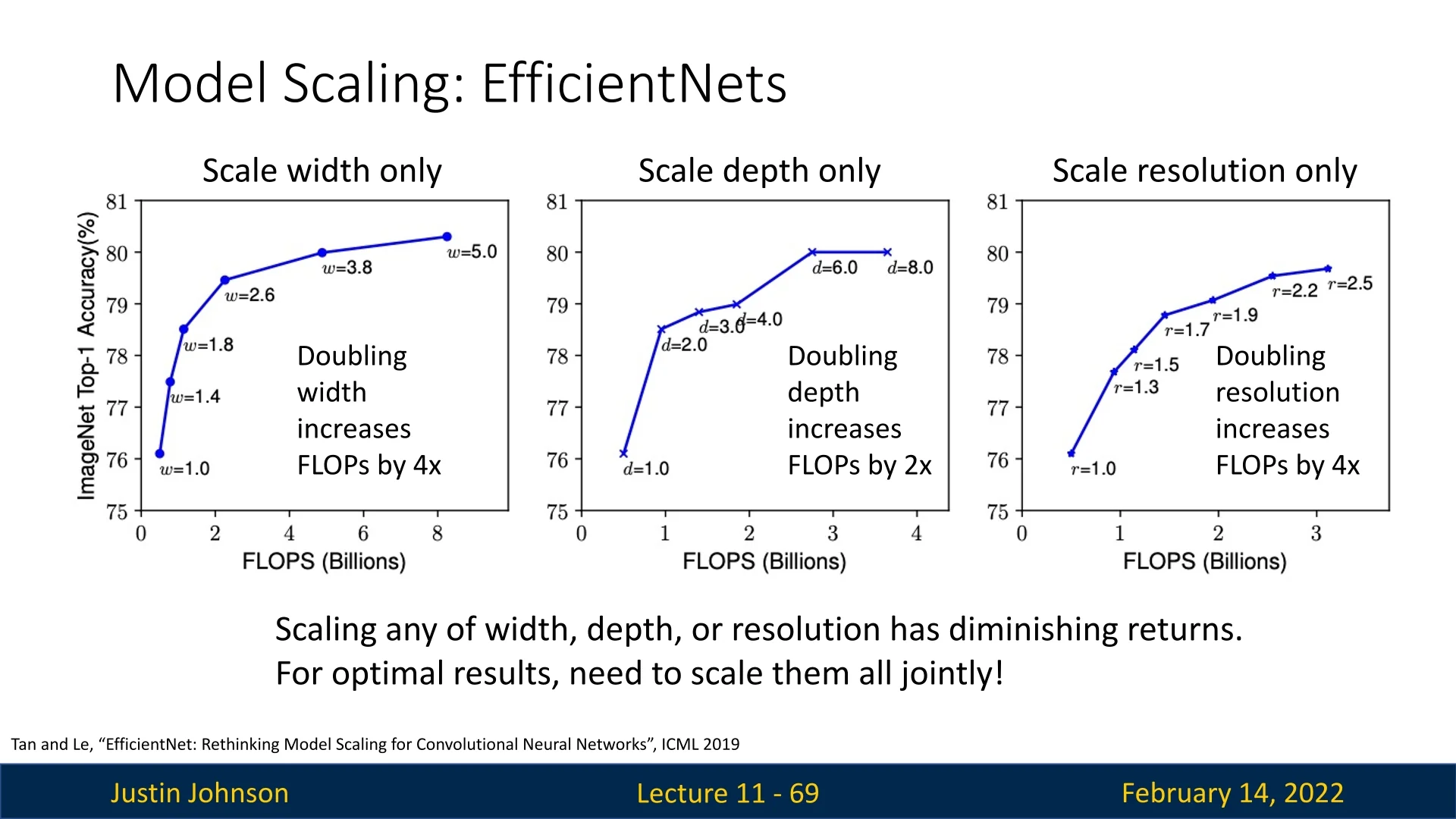
The Problem with Independent Scaling Scaling only one of these dimensions leads to diminishing returns. Excessive depth can cause vanishing gradients, extreme width increases make models harder to optimize, and excessive resolution scaling results in computational inefficiencies. Instead, EfficientNet optimally balances all three.
Furthermore, the different scaling dimensions are not independent:
- For higher-resolution images, increasing depth allows larger receptive fields to capture similar features that include more pixels.
- Increasing width enhances fine-grained feature extraction, allowing more expressive representations.
- Simply scaling one dimension in isolation is inefficient—scaling must be done in a coordinated manner to maximize the model’s performance-to-cost ratio.
11.6.2 How EfficientNet Works
EfficientNet introduces a compound scaling approach, which systematically scales width, depth, and resolution together. Instead of arbitrary scaling, EfficientNet determines the best scaling ratios using an optimization process.
Step 1: Designing a Baseline Architecture A well-optimized small model, called EfficientNet-B0, is first discovered using NAS (Neural Architecture Search). This model incorporates:
- Depthwise separable convolutions to reduce computational cost while preserving spatial feature extraction.
- Inverted residual blocks (from MobileNetV2), also known as MBConv blocks, which employ a narrow-wide-narrow structure for efficient processing.
- Squeeze-and-Excitation (SE) blocks to enhance channel-wise feature selection, improving accuracy with minimal overhead.
| Stage | Operator | Resolution | # Channels | # Layers |
|---|---|---|---|---|
| 1 | Conv3x3 | \(224 \times 224\) | 32 | 1 |
| 2 | MBConv1, k\(3\times 3\) | \(112 \times 112\) | 16 | 1 |
| 3 | MBConv6, k\(3\times 3\) | \(112 \times 112\) | 24 | 2 |
| 4 | MBConv6, k\(5\times 5\) | \(56 \times 56\) | 40 | 2 |
| 5 | MBConv6, k\(3\times 3\) | \(28 \times 28\) | 80 | 3 |
| 6 | MBConv6, k\(5\times 5\) | \(14 \times 14\) | 112 | 3 |
| 7 | MBConv6, k\(5\times 5\) | \(14 \times 14\) | 192 | 4 |
| 8 | MBConv6, k\(3\times 3\) | \(7 \times 7\) | 320 | 1 |
| 9 | Conv1x1 & Pooling & FC | \(7 \times 7\) | 1280 | 1 |
Step 2: Finding Optimal Scaling Factors Once the EfficientNet-B0 model is obtained, a grid search determines the best scaling factors for:
- \(\alpha \) (depth scaling).
- \(\beta \) (width scaling).
- \(\gamma \) (resolution scaling).
These scaling factors must satisfy the constraint: \[ \alpha \cdot \beta ^2 \cdot \gamma ^2 \approx 2 \] The reasoning behind this constraint is:
- It ensures that when we scale the model by a factor of \(\phi \), the total FLOPs increase by approximately \(2^\phi \), making it easier to monitor computational efficiency.
- This balance prevents over-scaling in one dimension while under-scaling in others, leading to more consistent improvements in accuracy per FLOP.
Through empirical search, the optimal values were found to be: \[ \alpha = 1.2, \quad \beta = 1.1, \quad \gamma = 1.15 \]
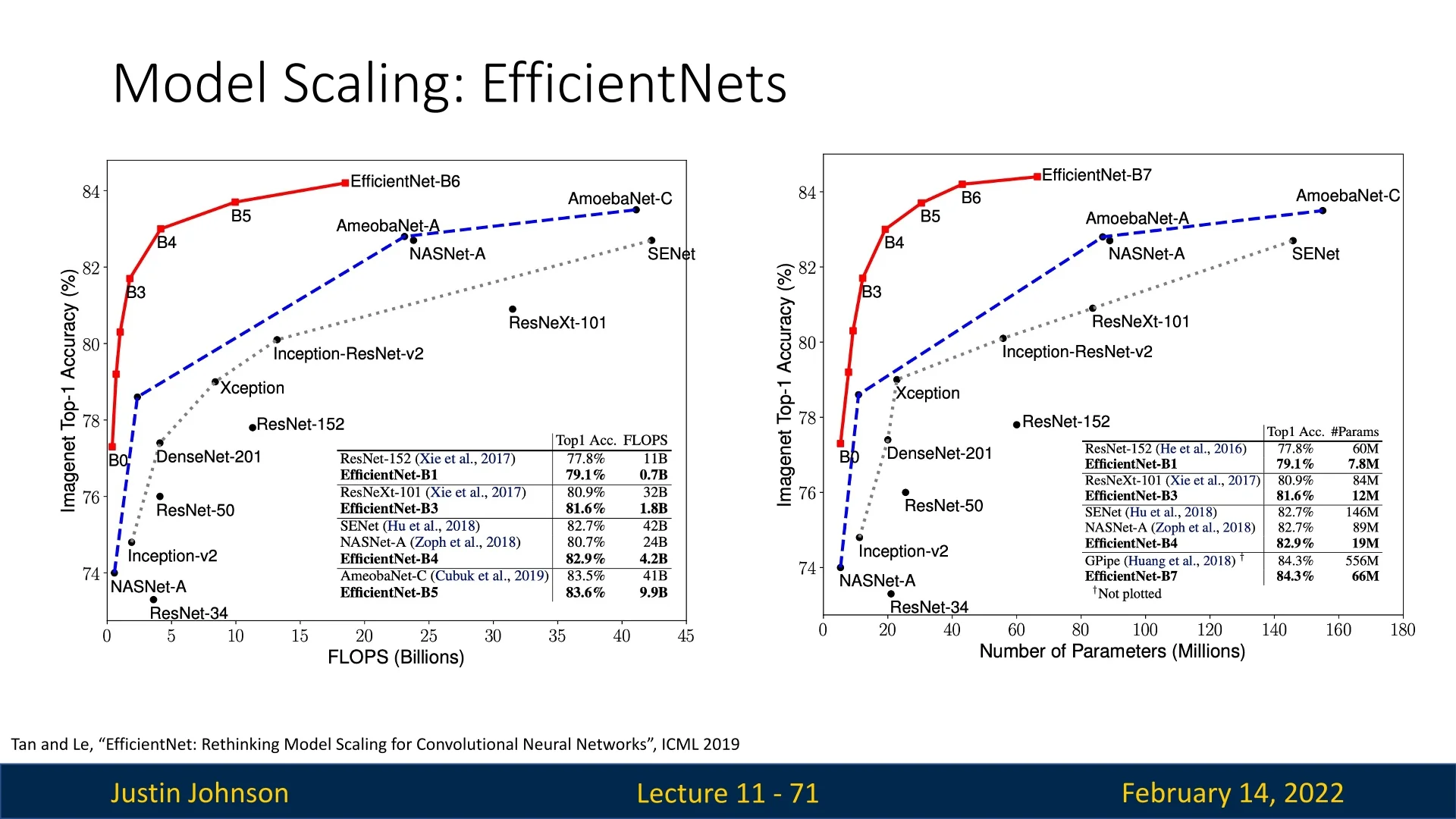
Step 3: Scaling to Different Model Sizes By applying these scaling factors to EfficientNet-B0 with different values of \(\phi \), a family of models is created:
- EfficientNet-B1 to EfficientNet-B7 scale up the base model by increasing depth, width, and resolution proportionally.
- This systematic scaling approach maintains computational efficiency while improving accuracy.
11.6.3 Why is EfficientNet More Effective
Balanced Scaling Improves Efficiency Unlike previous models that scale depth, width, or resolution separately, EfficientNet scales them together in a way that optimizes accuracy per FLOP.
Comparison with MobileNetV3 EfficientNet builds upon MobileNetV3’s NAS-based design but differs in:
- Optimized Scaling: MobileNetV3 relies on NAS to refine block structures, whereas EfficientNet applies compound scaling to improve overall architecture efficiency.
- Better Accuracy per FLOP: By jointly optimizing all scaling factors, EfficientNet achieves a better tradeoff than MobileNetV3.
- SE Blocks Across the Entire Network: Unlike MobileNetV3, which applies SE blocks selectively, EfficientNet integrates them at all relevant layers.
Comparison with Other Networks
- Compared to ResNets, EfficientNet achieves significantly higher accuracy per parameter.
- Compared to ShuffleNet, EfficientNet provides better optimization for real-world scenarios.
- Compared to MobileNetV2 and V3, EfficientNet systematically improves upon scaling while maintaining efficient building blocks.
11.6.4 Limitations of EfficientNet
Despite its efficiency in FLOPs, EfficientNet faces a major real-world issue: FLOPs do not directly translate to actual speed. Several factors impact real-world performance:
- Hardware Dependency: Runtime varies significantly across different devices (mobile CPU, server CPU, GPU, TPU).
- Depthwise Convolutions: While efficient on mobile devices, depthwise convolutions become memory-bound on GPUs and TPUs, leading to suboptimal execution times.
- Alternative Convolution Algorithms: Standard FLOP counting does not account for fast convolution implementations (e.g., FFT for large kernels, Winograd for \(3 \times 3\) convolutions), making direct FLOP comparisons misleading.
What’s Next? EfficientNetV2 and Beyond Since EfficientNet’s design focuses on FLOPs rather than actual hardware efficiency, researchers sought ways to improve real-world speed. This led to:
- EfficientNetV2: Improves inference speed and training efficiency.
- NFNets: Removes Batch Normalization for improved training stability (when working with a small mini-batch).
- ResNet-RS: A modernized ResNet with better scaling and training techniques.
- RegNets: Optimizes the macro architecture rather than just individual block designs.
Conclusion While EfficientNet represents a significant step forward in model scaling, its reliance on depthwise convolutions makes it suboptimal for GPUs and TPUs. Future architectures seek to address these limitations while maintaining high accuracy per FLOP.
Next, we explore EfficientNet-Lite, EfficientNetV2, which build upon EfficientNet’s strengths while improving real-world efficiency.
11.7 EfficientNet-Lite Optimizing EfficientNet for Edge Devices
11.7.1 Motivation for EfficientNet-Lite
While EfficientNet achieves an excellent balance between accuracy and computational cost, its deployment on edge devices (such as mobile phones and embedded systems) presents challenges. Many hardware accelerators used in mobile and IoT devices have limited support for certain EfficientNet components, leading to inefficiencies in real-world inference.
To address these limitations, EfficientNet-Lite [633] was introduced. It modifies EfficientNet’s architecture to improve execution speed on mobile and embedded hardware while maintaining high accuracy.
11.7.2 EfficientNet-Lite Architecture
EfficientNet-Lite is based on the original EfficientNet family but introduces several key modifications to enhance performance on edge devices:
- Removal of Squeeze-and-Excite (SE) Blocks SE blocks improve accuracy in EfficientNet, but they are not well supported by edge hardware. Removing them reduces latency and memory overhead.
- Replacement of Swish Activation with ReLU6 Swish, used in EfficientNet, is computationally expensive on mobile processors. ReLU6 is a simpler alternative that is better suited for low-power devices.
- Fixed Stem and Head Layers Instead of scaling the initial and final layers when increasing model size, EfficientNet-Lite keeps them fixed. This reduces computational complexity while keeping the network compact.
These optimizations result in five EfficientNet-Lite models, ranging in size from 5M to 13M parameters, offering various accuracy-speed trade-offs.
11.7.3 Performance and Comparison with Other Models
EfficientNet-Lite is designed to be a superior alternative to MobileNetV2 for edge devices, offering higher accuracy while maintaining efficiency. In comparison to ResNet, it achieves substantially faster inference times, making it more practical for real-world mobile applications.
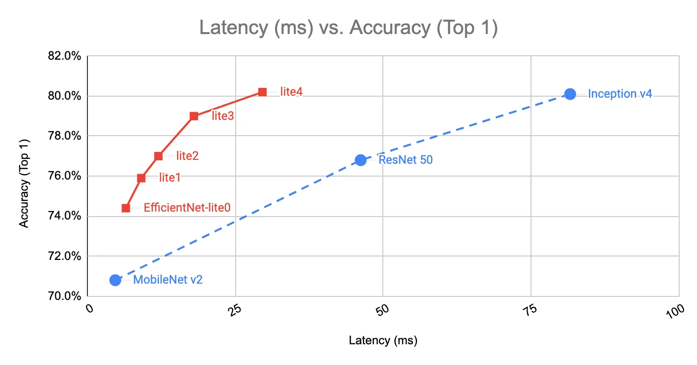
Model Size vs. Accuracy Trade-off EfficientNet-Lite models are designed to balance accuracy and efficiency better than previous mobile architectures. The comparison below illustrates how EfficientNet-Lite achieves superior accuracy with a relatively small model size compared to MobileNetV2 (that is a bit smaller) and ResNet (that is much larger):
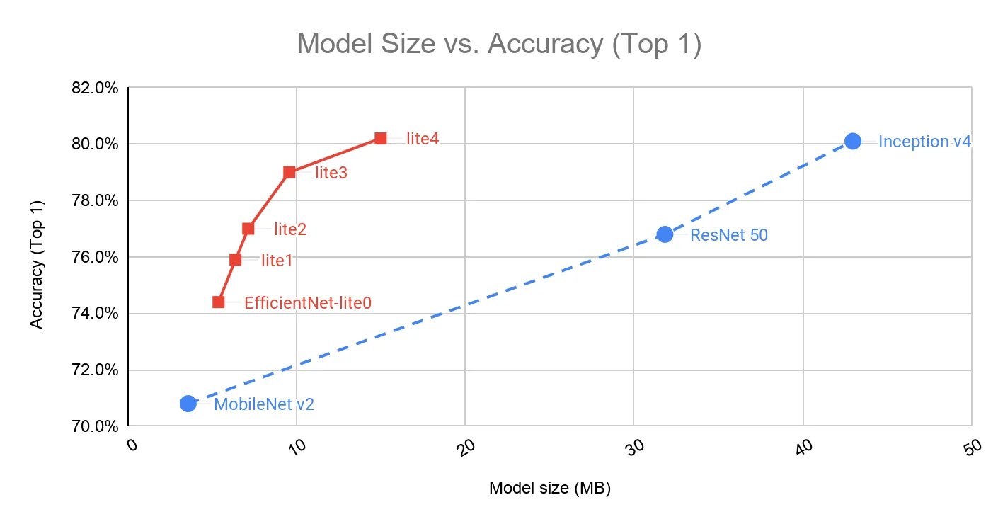
11.8 EfficientNetV2: Faster Training and Improved Efficiency
11.8.1 Motivation for EfficientNetV2
EfficientNetV1 introduced a highly parameter-efficient scaling approach, but it still had key inefficiencies:
- Slow training due to large image sizes: EfficientNetV1 aggressively scaled image resolution, which increased memory usage, forced smaller batch sizes, and significantly slowed training.
- Depthwise convolutions are inefficient in early layers: While depthwise convolutions reduce FLOPs, they do not fully utilize modern accelerators (e.g., GPUs, TPUs), leading to slow execution.
- Uniform scaling is suboptimal: EfficientNetV1 scaled all network stages equally, but different stages contribute unequally to accuracy and efficiency.
EfficientNetV2 [620] addresses these issues by introducing:
- Fused-MBConv blocks to replace depthwise convolutions in early layers, improving training speed.
- Progressive learning with adaptive regularization to accelerate training while maintaining accuracy.
- Non-uniform scaling to selectively increase depth in later network stages rather than scaling all layers equally.
11.8.2 Fused-MBConv: Improving Early Layers
A major efficiency bottleneck in EfficientNetV1 was the extensive use of depthwise convolutions, especially in early layers. While depthwise convolutions reduce parameters and FLOPs, they struggle to efficiently utilize hardware accelerators. EfficientNetV2 replaces depthwise convolutions in early layers with Fused-MBConv blocks.
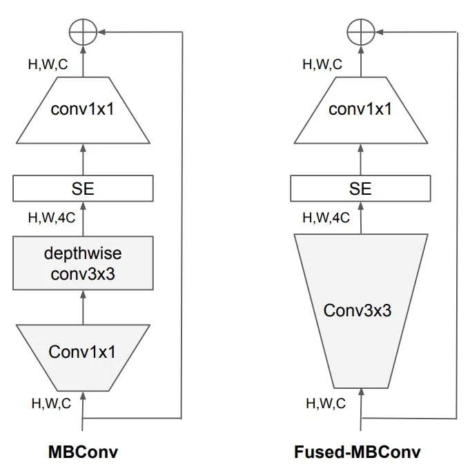
These blocks replace the separate \(1\times 1\) expansion and depthwise convolution layers with a single \(3\times 3\) convolution. The result:
- Faster execution on GPUs and TPUs due to better hardware utilization.
- Slightly higher FLOPs, but significantly reduced training time.
11.8.3 Progressive Learning: Efficient Training with Smaller Images
Training with large image sizes increases memory usage, forcing smaller batch sizes and slowing down training. EfficientNetV2 introduces progressive learning, where:
- Training starts with smaller images and weak regularization.
- As training progresses, image size gradually increases, and stronger regularization (e.g., dropout, RandAugment, MixUp) is applied.
This approach:
- Reduces memory usage, allowing for larger batch sizes (e.g., \(128\) vs. \(32\) on TPUv3, \(24\) vs. \(12\) on a V100).
- Speeds up training by up to \(2.2\times \) while maintaining or even improving accuracy.
11.8.4 FixRes: Addressing Train-Test Resolution Discrepancy
One key challenge in CNN training is the mismatch between the way images are processed during training and inference. EfficientNetV2 incorporates insights from FixRes [645] to mitigate this issue.
The Problem: Region of Classification (RoC) Mismatch
- During training, images are typically cropped randomly from larger images to introduce data diversity.
- During inference, a center crop is usually applied, leading to a distribution mismatch.
- This discrepancy can cause CNNs to struggle with scale invariance, degrading accuracy.
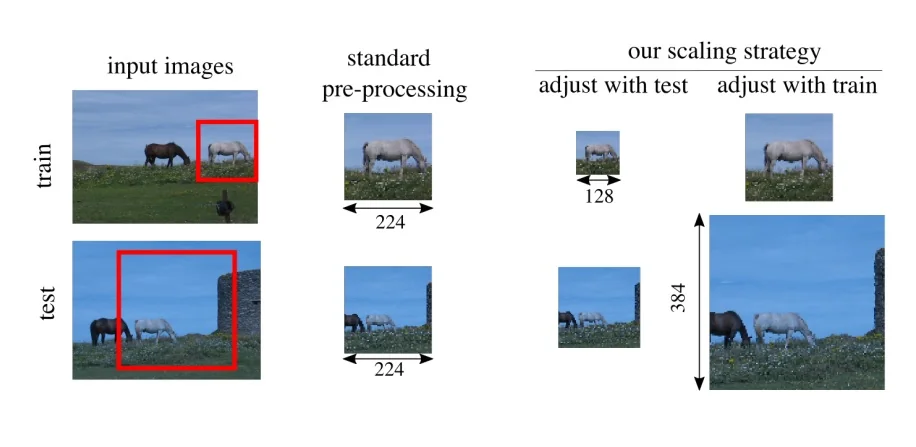
FixRes proposes two techniques to align train-test distributions:
- 1.
- Increasing the test-time crop size to better match training-time object sizes.
- 2.
- Fine-tuning the last few layers of the network using test-time preprocessing.
Implementation in EfficientNetV2
- EfficientNetV2 benefits from FixRes by aligning image resolutions across training and testing phases, improving robustness.
- Unlike the FixRes paper, EfficientNetV2 does not explicitly fine-tune post-training but incorporates similar resolution adjustments during training.
11.8.5 Non-Uniform Scaling for Improved Efficiency
EfficientNetV1 scaled width, depth, and resolution uniformly across all stages. However, different stages contribute differently to accuracy and efficiency.
EfficientNetV2 uses a non-uniform scaling strategy:
- More layers are added to later stages where deeper representations contribute more to accuracy.
- Maximum image resolution is capped at \(480\times 480\) to avoid excessive memory usage and slow training.
- The NAS search objective was updated to optimize for both accuracy and training efficiency, improving real-world execution.
11.8.6 EfficientNetV2 Architecture
EfficientNetV2 introduces three main model variants:
- EfficientNetV2-S: Smallest variant, optimized for efficient training and inference.
- EfficientNetV2-M: Medium variant balancing accuracy and efficiency.
- EfficientNetV2-L: Largest variant for high-accuracy tasks.
| Stage | Operator | Stride | Channels | Layers |
|---|---|---|---|---|
| 0 | Conv3x3 | 2 | 24 | 1 |
| 1 | Fused-MBConv1, k3x3 | 1 | 24 | 2 |
| 2 | Fused-MBConv4, k3x3 | 2 | 48 | 4 |
| 3 | Fused-MBConv4, k3x3 | 2 | 64 | 4 |
| 4 | MBConv4, k3x3, SE0.25 | 2 | 128 | 6 |
| 5 | MBConv6, k3x3, SE0.25 | 1 | 160 | 9 |
| 6 | MBConv6, k3x3, SE0.25 | 2 | 256 | 15 |
| 7 | Conv1x1 & Pooling & FC | - | 1280 | 1 |
11.8.7 EfficientNetV2 vs. EfficientNetV1
EfficientNetV2 improves upon EfficientNetV1 in several ways:
- Faster Training: Progressive learning and FixRes improve training speed by up to \(11\times \).
- Better Hardware Utilization: Fused-MBConv accelerates training by replacing inefficient depthwise convolutions in early layers.
- Improved Scaling: Non-uniform scaling provides better efficiency than EfficientNetV1’s uniform scaling.
11.8.8 EfficientNetV2 vs. Other Models
EfficientNetV2 is designed for improved training speed, parameter efficiency, and inference performance. The following table compares it to prior convolutional and transformer-based architectures using ImageNet Top-1 accuracy, model size, compute cost, and latency.
| Model | Top-1 | Params | FLOPs | Infer | Train |
|---|---|---|---|---|---|
| (%) | (M) | (B) | (ms) | (hrs) | |
ConvNets / Hybrid |
|||||
| EffNet-B3 [15] | 81.5 | 12 | 1.9 | 9 | 3.1 |
| EffNet-B4 [15] | 82.9 | 19 | 4.2 | 10 | 6.2 |
| EffNet-B5 [15] | 83.6 | 30 | 9.9 | 14 | 12 |
| RegNetY-8GF [19] | 82.9 | 39 | 8.0 | 16 | 3.4 |
| RegNetY-16GF [19] | 83.4 | 84 | 16.0 | 24 | 6.8 |
| ResNeSt-101 [20] | 83.0 | 48 | 11.0 | 20 | 3.8 |
| ResNeSt-200 [20] | 83.8 | 66 | 15.0 | 25 | 5.9 |
| NFNet-F0 [21] | 83.6 | 72 | 12.0 | 30 | 8.9 |
| NFNet-F1 [21] | 84.7 | 132 | 35.0 | 42 | 21 |
Vision Transformers |
|||||
| DeiT-B [22] | 81.8 | 86 | 17.0 | 33 | – |
| ViT-B/16 [23] | 77.9 | 86 | 55.0 | 36 | – |
EfficientNetV2 (Ours) |
|||||
| EffNetV2-S | 83.9 | 22 | 8.8 | 24 | 2.9 |
| EffNetV2-M | 85.1 | 55 | 24.0 | 54 | 11 |
| EffNetV2-L | 85.7 | 120 | 53.0 | 98 | 21 |
| EffNetV2-S (21k) | 85.9 | 22 | 8.8 | 24 | 5.2 |
| EffNetV2-M (21k) | 86.7 | 55 | 24.0 | 54 | 15 |
| EffNetV2-L (21k) | 87.3 | 120 | 53.0 | 98 | 34 |
Key Observations:
- EfficientNetV2 achieves substantially higher accuracy than lightweight models like MobileNet and ShuffleNet, but with increased compute. While MobileNetV1, MobileNetV2, MobileNetV3, and ShuffleNetV2 prioritize minimal parameters and ultra-fast inference for mobile scenarios, their Top-1 accuracies remain below 76%. In contrast, EfficientNetV2-S achieves 83.9% accuracy with a moderate compute footprint (22M parameters, 8.8B FLOPs), making it well-suited for high-accuracy applications with relaxed latency constraints.
- EfficientNetV2-S outperforms DeiT-S in both accuracy and real-world latency. Despite comparable model sizes and FLOPs, EfficientNetV2-S achieves 2.1% higher accuracy than DeiT-S (83.9% vs. 81.8%) and is significantly faster during inference (24ms vs. 33ms). This highlights the practical efficiency gap between convolutional networks and vision transformers, especially in small-to-medium compute regimes.
- EfficientNetV2 offers better accuracy–efficiency tradeoffs than RegNetY variants. For instance, RegNetY-8GF and EfficientNetV2-S have similar latency (16–24ms) and parameter counts (39M vs. 22M), yet EfficientNetV2-S surpasses RegNetY-8GF by 1.0% in accuracy. This demonstrates that EfficientNetV2’s compound scaling and progressive learning strategy yield superior results under comparable computational budgets.
Training Speed and Efficiency EfficientNetV2 significantly reduces training time compared to EfficientNetV1, as shown in Table 11.10.
- EfficientNetV2 achieves higher accuracy with lower FLOPs compared to its fitting variants of EfficientNetV1.
- Training time is improved by up to 11×, while also reducing the number of epochs required for convergence.
- Optimizations such as Fused-MBConv and progressive learning enable significantly faster training and inference.
11.9 NFNets: Normalizer-Free ResNets
11.9.1 Motivation: Why Do We Need NFNets?
Deep networks like ResNets rely heavily on Batch Normalization (BN) to stabilize training. BN is effective because it:
- Stabilizes gradients, enabling deep networks to train reliably.
- Reduces sensitivity to learning rates and initialization schemes.
- Acts as implicit regularization, improving generalization.
- Has zero inference cost, since BN statistics are merged into preceding layers.
However, BN also has major drawbacks:
- Incompatible with small batch sizes: BN estimates mean and variance over a batch, leading to instability when batches are too small.
- Different behavior at training and inference: BN tracks running statistics during training, which may not match the distribution at inference.
- Slows training: BN introduces additional computation and memory overhead.
To address these issues, NFNets [54] remove BN entirely while preserving training stability. However, removing BN introduces another challenge: variance explosion in residual networks.
11.9.2 Variance Explosion Without BatchNorm
Variance Scaling in Residual Networks A typical residual block in a ResNet has the form \[ x_{\ell +1} = f_{\ell }(x_{\ell }) + x_{\ell }. \] While this skip connection aids gradient flow, it also can accumulate variance at each stage: \[ \operatorname {Var}\bigl (x_{\ell +1}\bigr ) \,\approx \, \operatorname {Var}\bigl (x_{\ell }\bigr )\;+\;\operatorname {Var}\bigl (f_{\ell }(x_{\ell })\bigr ). \] In deep architectures, repeated accumulation can cause a variance explosion, destabilizing activations.
Role of Weight Initialization Careful initialization is a common strategy to keep activations in check at the start of training. As we’ve seen, Fixup Initialization [790] modifies weight scaling and learning rates in residual blocks. However, while Fixup prevents variance from exploding early on, it does not guarantee stability throughout the entire training if the network is very deep. Thus, batch normalization historically enabled deeper ResNets by continuously regulating activation variance during training, not just at initialization.
11.9.3 Why Not Rescale the Residual Branch?
One idea to tame variance is to explicitly rescale the residual output: \begin {equation} x_{\ell +1} \;=\; x_{\ell } \;+\;\alpha \; f_{\ell }\!\Bigl (\,\frac {x_{\ell }}{\beta _{\ell }}\Bigr ), \end {equation} where \(\alpha \) is a learned or fixed scaling factor, and \[ \beta _{\ell } \;=\;\sqrt {\operatorname {Var}(x_{\ell })} \] normalizes the input. This reparameterization implies \[ \operatorname {Var}(x_{\ell +1}) \;\approx \; \operatorname {Var}(x_{\ell }) \;+\; \alpha ^2, \] limiting variance accumulation per layer.
In practice, however, this approach faces two major hurdles:
- Sensitivity to \(\alpha \): Choosing or tuning \(\alpha \) is non-trivial; a suboptimal setting can harm training stability.
- Long-Term Drift: Even with rescaling at each layer, subtle interactions over many layers can still lead to drift in variance.
11.9.4 NFNets: Weight Normalization Instead of BN
To avoid using batch-dependent statistics, NFNets employ a weight normalization procedure at every training step. Rather than normalizing layer outputs (as in BN), NFNets normalize convolutional filters directly. Concretely, for each convolutional weight tensor \(\mathbf {W}\) of shape \(\mbox{(out_channels)} \times \mbox{(in_channels)} \times K \times K\), they compute:
\[ \widehat {W}_{i,j} \;=\; \gamma \,\cdot \, \frac {W_{i,j} \;-\; \operatorname {mean}(\mathbf {W}_{i,\cdot })}{\operatorname {std}(\mathbf {W}_{i,\cdot }) \,\sqrt {N}}, \] where:
- \(W_{i,j}\) is the \((i,j)\)-th weight parameter (for the \(i\)-th output channel and \(j\)-th element within that channel’s kernel).
- \(\operatorname {mean}(\mathbf {W}_{i,\cdot })\) and \(\operatorname {std}(\mathbf {W}_{i,\cdot })\) are the mean and standard deviation of all weights in output channel \(i\).
- \(N = K^2 \,C_{\mathrm {in}}\) is the fan-in of the kernel, i.e. the total number of input elements for a single filter.
- \(\gamma \) is a channel-wise scaling constant. For ReLU, a recommended choice is \[ \gamma \;=\; \sqrt {\frac {2}{\,1 - (1/\pi )\,}} \;\approx \; 1.38, \] reflecting the variance constraints needed to maintain stable activations.
Why This Works By standardizing each filter to have zero mean and unit variance (up to a fixed scale \(\gamma \)), NFNets ensure that layer outputs do not escalate in variance purely because of unbounded filter norms. This effectively replaces BN’s role of keeping activations well-conditioned:
- No Batch Statistics: The normalization depends solely on parameters themselves, not on the running or batch-dependent means/variances of activations.
- Stable Training Without BN: Controlling filter norms across all layers prevents activation blow-up or collapse, thereby stabilizing the forward pass and facilitating gradient flow in the backward pass.
- No Extra Inference Overhead: Once the filters have been normalized during training, the final weights \(\widehat {W}\) remain fixed for inference. There are no additional computations per input sample, just as BN adds no overhead at inference time.
Relation to Earlier Weight Standardization NFNets’ approach is reminiscent of “Weight Standardization” and other filter-centric normalization methods, yet NFNets further incorporate factors like \(\gamma \) to preserve proper variance for ReLU (or other activations). This synergy helps to match or exceed the performance of BN-equipped networks, while obviating the need for large batch sizes or running-mean tracking.
11.9.5 NFNets Architecture and ResNet-D
NFNets build upon a modified ResNet architecture known as ResNet-D [221]. This includes:
- Improved stem layer: Uses an initial \( 3 \times 3 \) convolution followed by an average pooling layer for better downsampling.
- Enhanced downsampling blocks: Applies pooling before strided convolutions to smooth feature transitions.
- Increased group width: Uses 128 channels per group to improve feature expressiveness.
NFNets further introduce:
- Adaptive Gradient Clipping (AGC): Dynamically clips gradients if they exceed a predefined threshold, preventing instability.
- Stronger regularization: Includes MixUp, RandAugment, CutMix, DropOut, and Stochastic Depth to enhance generalization.
11.9.6 Comparison Across Diverse Architectures
To contextualize NFNets among other leading models—spanning RegNets, efficient CNNs, and Transformers. The following table presents key metrics such as FLOPs, parameter counts, training and inference times, and top-1 accuracy on ImageNet. The data is aggregated from publicly reported benchmarks in [620, 54, 514, 788, 134, 647], among others. Where possible, all inference times are measured under the same setup (NVIDIA V100 GPU, FP16 precision, batch size 16) unless explicitly noted.
| Model | Resolution | Top-1 (%) | Params (M) | FLOPs (B) | Inference Time (ms, V100) | Train Time (hrs, TPU) |
|---|---|---|---|---|---|---|
Selected CNN Baselines |
||||||
| ResNet-50 [215] | 224 | 76.1 | 26 | 4.1 | – | – |
| RegNetY-16GF [514] | 224 | 82.9 | 84 | 16.0 | 32 | – |
| NFNet-F0 [54] | 256 | 83.6 | 72 | 12.4 | 56.7 | 8.9 |
| NFNet-F1 [54] | 256 | 84.7 | 133 | 35.5 | 133.9 | 20 |
EfficientNet Family |
||||||
| EfficientNet-B4 [621] | 380 | 82.9 | 19 | 4.2 | 30 | 21 |
| EfficientNet-B7 [621] | 600 | 84.7 | 66 | 38.0 | 170 | 139 |
| EfficientNetV2-S [620] | 384 | 83.9 | 22 | 8.8 | 24 | 7.1 |
| EfficientNetV2-M [620] | 480 | 85.1 | 54 | 24.0 | 57 | 13 |
| EfficientNetV2-L [620] | 480 | 85.7 | 120 | 53.0 | 98 | 24 |
Transformer-Based Models |
||||||
| ViT-B/16 [134] | 384 | 77.9\(^\dagger \) | 86 | 55.5 | 68 | – |
| DeiT-S [647] | 224 | 79.8 | 22 | 4.6 | – | – |
| DeiT-B [647] | 224 | 81.8 | 86 | 18.0 | – | – |
- NFNet eliminates batch normalization while maintaining high accuracy. By normalizing weights instead of activations, NFNets improve stability and remove BN’s reliance on batch size.
- EfficientNetV2 balances FLOPs, accuracy, and training speed. Compared to NFNet, EfficientNetV2 achieves high accuracy while optimizing FLOPs and training efficiency, making it ideal for real-world deployment.
- RegNets provide a competitive alternative. RegNetY-16GF balances FLOPs and accuracy well, but it still relies on BN for stability.
- Vision Transformers (ViTs) trade efficiency for flexibility. DeiT-S and ViT-B require significantly more FLOPs for similar accuracy levels and suffer from higher inference times due to less optimized self-attention operations. Nevertheless, as we’ll later see, when trained on larger datasets or used in bigger architectures, can perform very well in many CV problems.
- Training time is a critical differentiator. NFNet variants require significantly less training time compared to large EfficientNet or Transformer-based models, making them attractive for rapid deployment.
- Higher resolutions increase FLOPs and accuracy. Many NFNet and EfficientNet variants are trained at larger resolutions (\(256\times 256\) or higher), leading to improved accuracy but increased computational cost.
11.9.7 Further Reading and Resources
For a more intuitive explanation of NFNets, including their theoretical foundations and practical implications, I recommend watching Yannic Kilcher’s breakdown of the NFNet architecture. His video provides insights into variance scaling, weight normalization, and why NFNets achieve competitive results without batch normalization.
- Yannic Kilcher: “NFNets – Normalizer-Free Neural Networks” ( YouTube Video)
This video complements the material covered in this section by offering an accessible and engaging perspective on the core concepts behind the architecture.
11.10 Revisiting ResNets: Improved Training and Scaling Strategies
Bello et al. (2021) [34] revisit the ResNet architecture and propose a series of improvements that significantly boost performance through better training strategies and scaling methodologies. Their approach demonstrates that ResNets can match or surpass EfficientNets when trained effectively.
11.10.1 Training Enhancements for ResNets
Starting from a baseline ResNet-200, the authors apply several training improvements. The following table summarizes how each change contributes to accuracy gains:
| Modification | Top-1 Accuracy (%) | Accuracy Gain |
|---|---|---|
| Baseline ResNet-200 | 79.0 | – |
| + Cosine LR decay | 79.3 | +0.3 |
| + Longer training (90 \(\rightarrow \) 350 epochs) | 78.8 | -0.5 |
| + EMA of weights | 79.1 | +0.3 |
| + Label smoothing | 80.4 | +1.3 |
| + Stochastic Depth | 80.6 | +0.2 |
| + RandAugment | 81.0 | +0.4 |
| + Dropout on FC layer | 80.7 | -0.3 |
| + Less weight decay | 82.2 | +1.5 |
| + Squeeze-and-Excite (SE) blocks | 82.9 | +0.7 |
| + ResNet-D modifications | 83.4 | +0.5 |
- Cosine Learning Rate Decay: Adjusts the learning rate smoothly over training, improving convergence.
- Exponential Moving Average (EMA) of Weights: Stabilizes training by averaging weights over time.
- Stochastic Depth: Randomly drops entire layers during training to improve generalization.
- RandAugment: Data augmentation technique that enhances image diversity during training.
- Squeeze-and-Excite (SE) Blocks: Improves channel-wise feature recalibration.
- ResNet-D Modifications: Includes better downsampling strategies to improve feature representation.
11.10.2 Scaling ResNets for Efficient Training
Beyond training strategies, the study explores scaling ResNets effectively, optimizing width, depth, and input resolution to generate networks of various sizes. Instead of using an expensive NAS-based search, the authors brute-force search over:
- Network Width: Initial widths scaled by \(0.25\times \), \(0.5\times \), \(1.0\times \), \(1.5\times \), or \(2.0\times \) the baseline.
- Depth: Networks evaluated at 26, 50, 101, 200, 300, 350, and 400 layers.
- Input Resolution: Tested at 128, 160, 224, 320, and 448 pixels.
11.10.3 ResNet-RS vs. EfficientNet: A Re-Evaluation
This work challenges the prevailing assumption that EfficientNets are the most optimal CNN models, showing that properly trained ResNets can achieve comparable or superior accuracy while training significantly faster than EfficientNets.
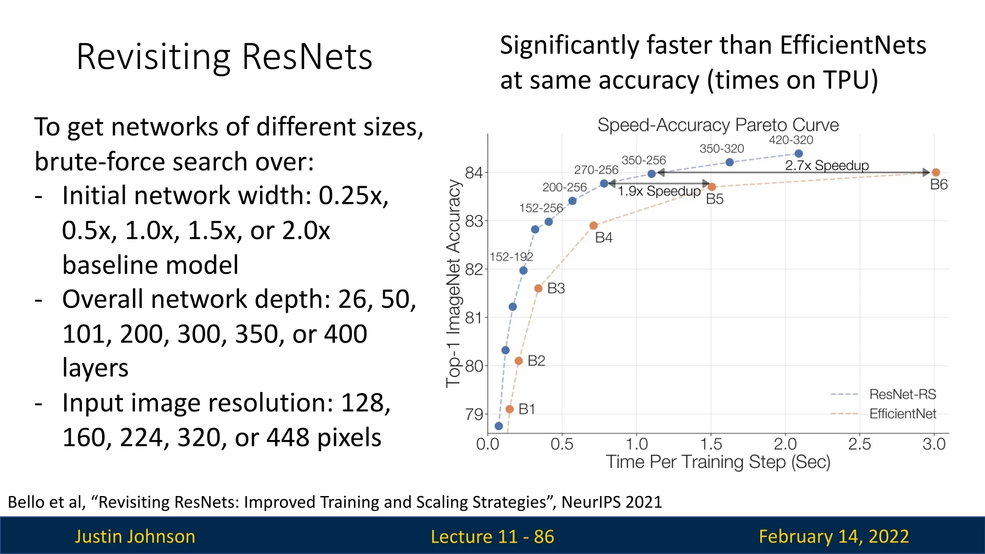
Comparison of ResNet-RS and EfficientNet Although EfficientNets minimize FLOPs while maintaining high accuracy, ResNet-RS models demonstrate that with optimized scaling and training strategies, ResNets remain highly competitive in both accuracy and efficiency. The following table provides a comparison of ResNet-RS and EfficientNet in terms of accuracy, parameters, FLOPs, memory usage, and inference latency.
| Model | Resolution | Top-1 Acc. (%) | Params (M) | FLOPs (B) | TPU Latency (s) | TPU Memory (GB) | V100 Latency (s) |
|---|---|---|---|---|---|---|---|
| ResNet-RS-350 | 256 | 84.0 | 164 | 69 | 1.1 | 7.3 | 4.7 |
| EfficientNet-B6 | 528 | 84.0 | 43 (3.8\(\times \)) | 38 (1.8\(\times \)) | 3.0 (2.7\(\times \)) | 16.6 (2.3\(\times \)) | 15.7 (3.3\(\times \)) |
| ResNet-RS-420 | 320 | 84.4 | 192 | 128 | 2.1 | 15.5 | 10.2 |
| EfficientNet-B7 | 600 | 84.7 | 66 (2.9\(\times \)) | 74 (1.7\(\times \)) | 6.0 (2.9\(\times \)) | 28.3 (1.8\(\times \)) | 29.9 (2.8\(\times \)) |
- ResNet-RS models have more FLOPs and parameters but train and infer faster. Due to architectural refinements and training optimizations, ResNet-RS achieves competitive accuracy with significantly lower latency.
- ResNet-RS optimizations improve memory efficiency. Despite higher parameter counts, ResNet-RS models consume less memory than EfficientNets, making them easier to deploy at scale.
- Scaling strategies differ: EfficientNet follows NAS-derived compound scaling, whereas ResNet-RS employs brute-force search over depth, width, and input resolution to optimize for real-world efficiency. This approach is much easier and practical in comparison.
Conclusion While EfficientNets have been widely adopted due to their optimized scaling, [34] demonstrates that properly scaled and trained ResNets can remain highly competitive. These findings suggest that ResNets can achieve state-of-the-art results with faster training and inference, making them a strong alternative to NAS-based architectures like EfficientNet.
11.11 RegNets: Network Design Spaces
Motivation: Designing Scalable Architectures
While models like improved ResNets and EfficientNets have demonstrated strong
performance, they rely on either manual design or costly NAS-based searches.
RegNets [514] propose a structured approach to network design by defining a
parameterized design space that enables automatic discovery of efficient
architectures.
11.11.1 RegNet Architecture
RegNets follow a simple architectural structure:
- A stem consisting of a single \(3 \times 3\) convolution.
- A body composed of four stages, each containing multiple blocks.
- A head with global pooling and a final classification layer.
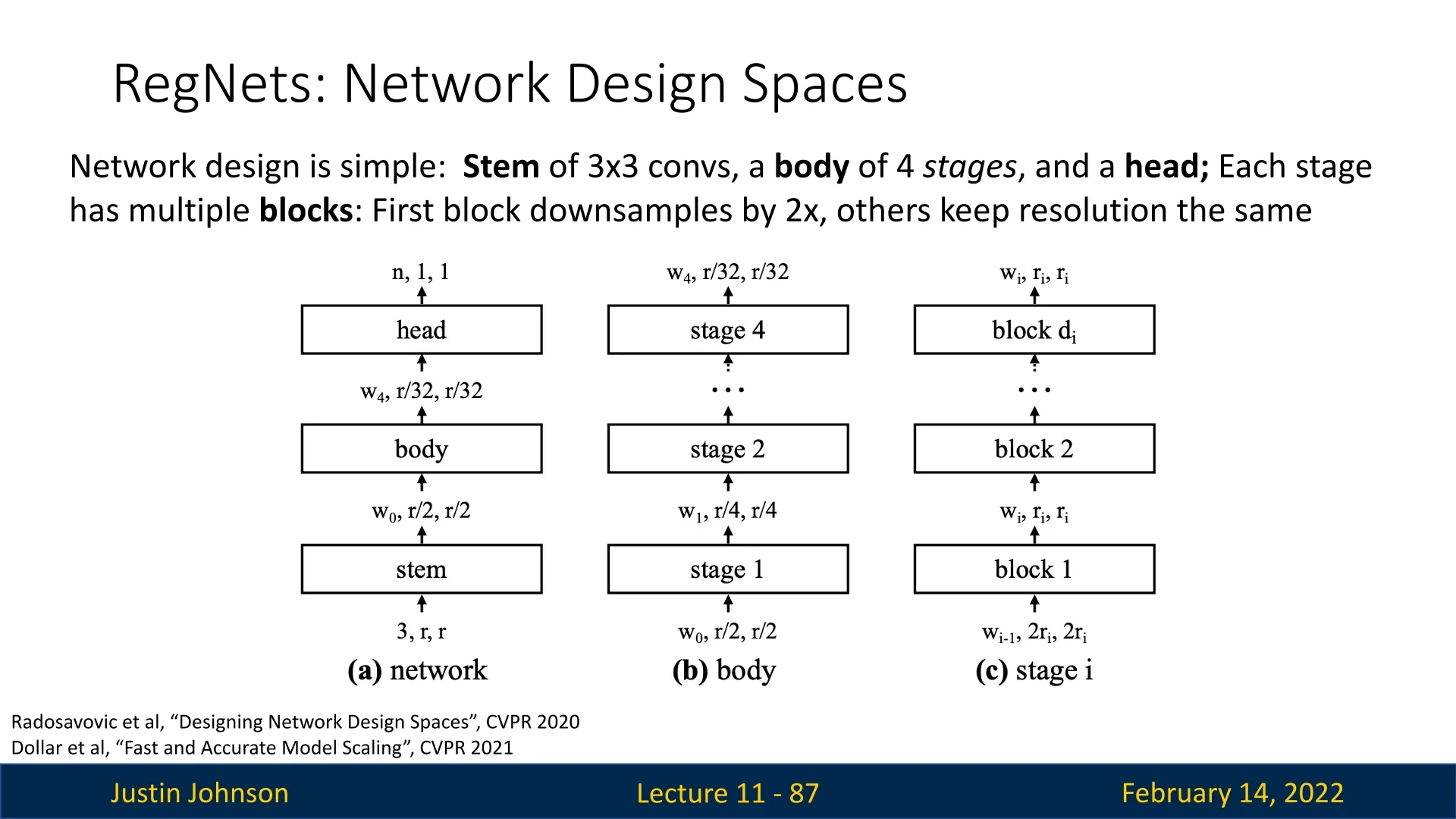
Within each stage, the first block downsamples the feature maps by a factor of 2, while the remaining blocks maintain spatial resolution.
Block Design: Generalizing ResNeXt Each RegNet stage is parameterized by:
- Number of blocks per stage.
- Number of input channels \(w\).
- Bottleneck ratio \(b\) (determines expansion factor).
- Group width \(g\) (number of channels per group).
This flexible parameterization generalizes ResNeXt, allowing for a controlled exploration of network architectures.
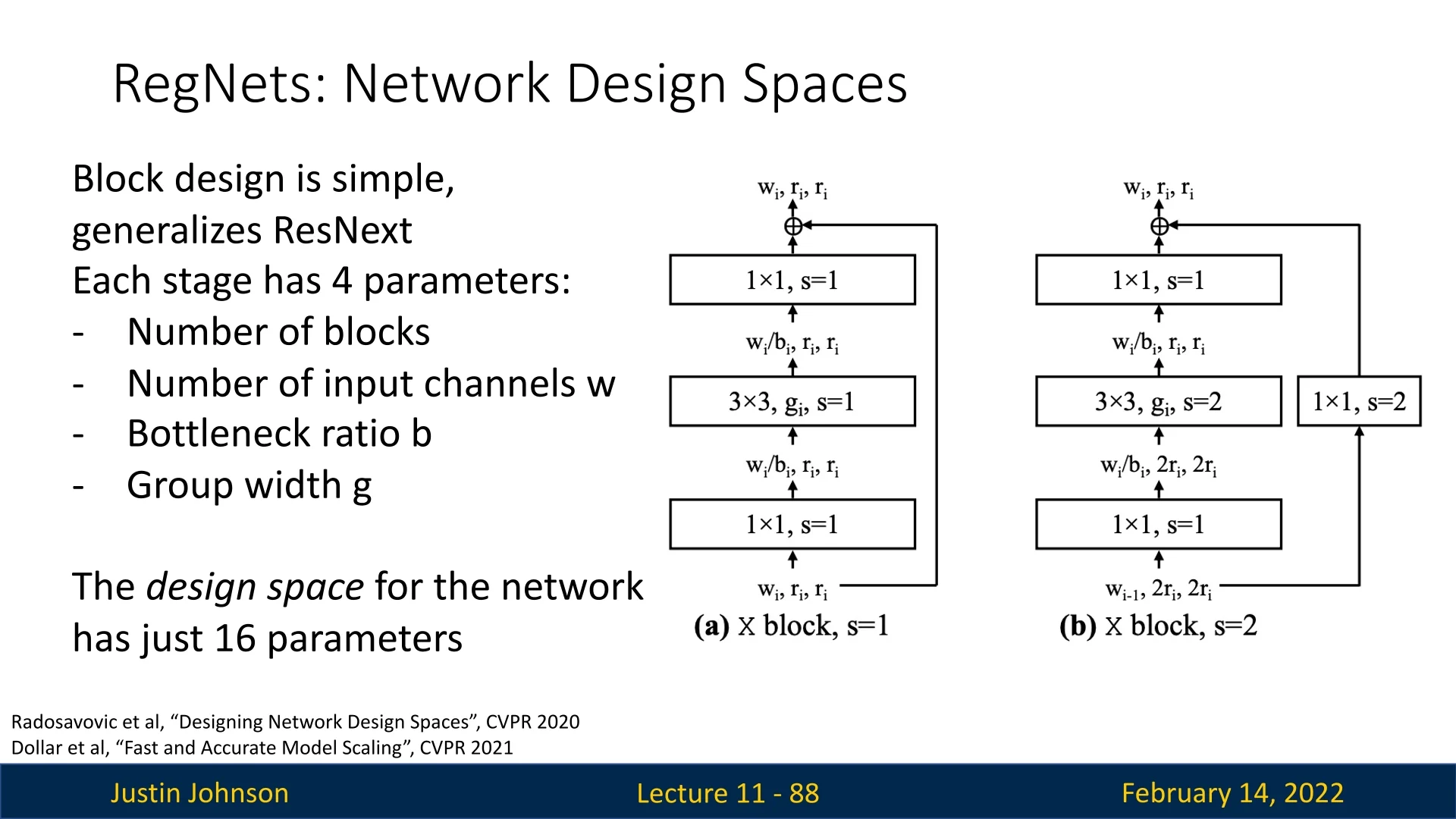
11.11.2 Optimizing the Design Space
Defining the Initial Design Space
RegNets aim to find optimal architectures by systematically searching over a
well-defined design space rather than relying on manual design or costly NAS
searches. Initially, each RegNet model consists of four stages, where each stage
is parameterized by:
- Number of blocks per stage.
- Number of input channels \(w\).
- Bottleneck ratio \(b\) (ratio of expanded channels within each bottleneck block).
- Group width \(g\) (number of channels per group in grouped convolutions).
Since each of the four stages has these four parameters, the total design space initially consists of 16 parameters.
Random Sampling and Performance Trends To refine this large design space, the authors of [514] employed a random sampling approach:
- Randomly generate a large number of architectures by varying the 16 parameters.
- Train and evaluate these architectures to identify general performance trends.
By analyzing these trends, they discovered that some degrees of freedom were unnecessary, and simplifying the design space led to more efficient and generalizable architectures.
Reducing the Design Space Based on observed trends, they progressively reduced the search space from 16 parameters to just 6:
- Bottleneck ratio is shared across all stages (16 \(\rightarrow \) 13 parameters).
- Group width is shared across all stages (13 \(\rightarrow \) 10 parameters).
- Width and block count per stage increase linearly, rather than being freely chosen (10 \(\rightarrow \) 6 parameters).
Final Six Parameters The final, refined design space consists of only six parameters, making it significantly easier to search for high-performing models:
- Overall depth (\(d\)) – total number of layers.
- Bottleneck ratio (\(b\)) – controls the internal channel expansion within each block.
- Group width (\(g\)) – defines the number of groups in grouped convolutions.
- Initial width (\(w_0\)) – number of channels in the first stage.
- Width growth rate (\(w_a\)) – rate at which channels expand between stages.
- Blocks per stage (\(w_m\)) – number of blocks in each stage.
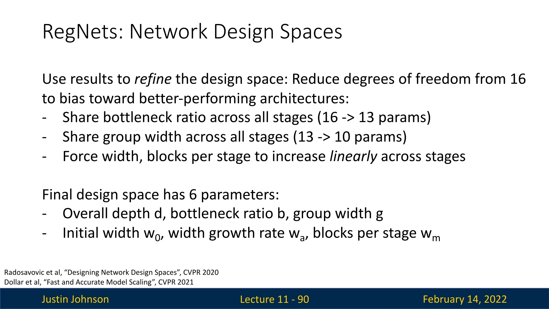
Why This Works By simplifying the search space, RegNets maintain flexibility while reducing complexity, leading to models that:
- Are easier to optimize, requiring fewer trial-and-error experiments.
- Generalize better, as the imposed structure aligns with observed empirical trends.
- Can be searched efficiently, finding optimal models faster than traditional NAS approaches.
Conclusion Through a structured reduction of the design space, RegNets provide a systematic approach to architecture search, yielding high-performing models without the inefficiencies of exhaustive NAS.
11.11.3 Performance and Applications
RegNets yield highly competitive architectures:
- Random search finds strong models across different FLOP budgets.
- RegNet achieves similar accuracy to EfficientNets while training up to 5\(\times \) faster per iteration.
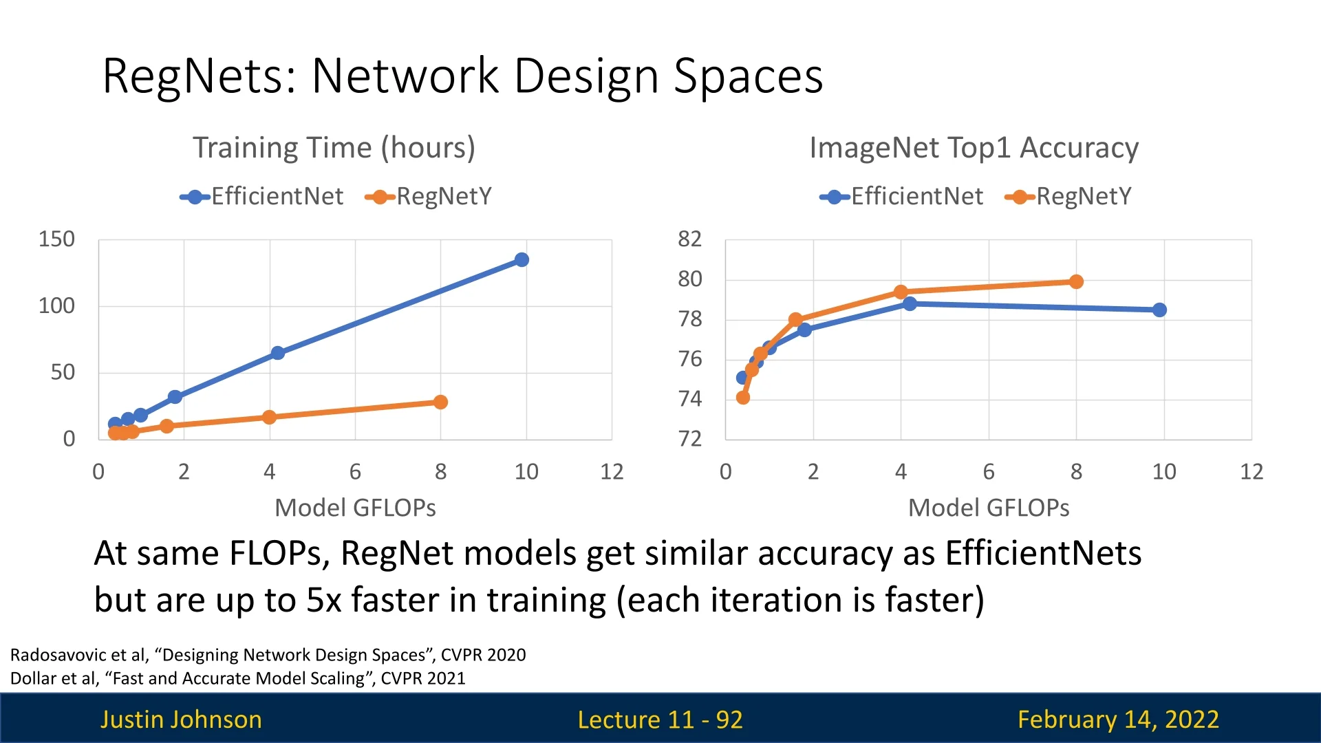
Beyond academic benchmarks, RegNets have been deployed in real-world applications, such as Tesla’s autonomous driving system, where they efficiently process inputs from multiple cameras.
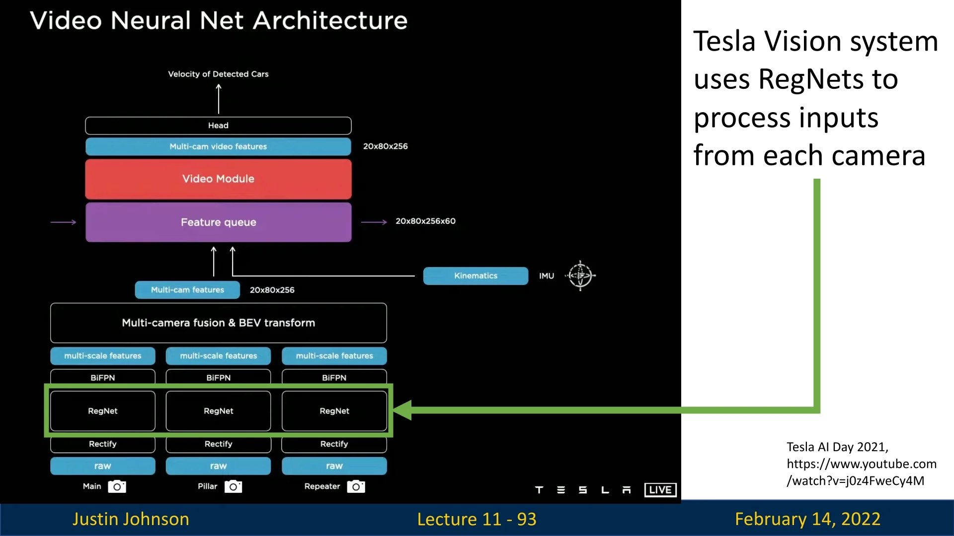
- RegNets provide a structured approach to architecture search, reducing manual design effort while yielding efficient models.
- Refining the design space leads to better architectures, as random search alone is inefficient.
- RegNets achieve EfficientNet-level accuracy with significantly faster training, making them practical for deployment.
- RegNets are already in use in real-world applications, demonstrating their robustness and efficiency.
Conclusion RegNets present an automated yet efficient approach to neural architecture search, demonstrating that careful design-space refinement can lead to highly competitive architectures. By leveraging structured scaling rules, RegNets achieve strong accuracy-FLOP trade-offs while being significantly faster to train than EfficientNets.
Enrichment 11.12: The Modern ConvNet Renaissance
Beyond the ResNet era. By the early 2020s, the landscape of convolutional neural networks appeared mature. The ingredients introduced previously in this document—residual connections (ResNets), multi-branch modules (Inception), depthwise separable convolutions and inverted bottlenecks (MobileNet), squeeze-and-excitation (SENet), and compound scaling (EfficientNet)—had coalesced into a stable hierarchy of backbones for classification and dense prediction. At the same time, Vision Transformers (ViTs) and Swin-like architectures began to dominate leaderboards, not because convolutions were inherently inferior, but because transformer models benefited from carefully tuned macro-designs (stage layouts, patch stems, normalization/activation choices) and strong training recipes.
In response, a “third wave” of ConvNets emerged. These architectures do not discard convolutions; instead, they re-express ConvNets in a language compatible with ViTs and modern hardware. This enrichment gives a high-level map of that design space. In the following, we will return to these ideas in detail: ConvNeXtV2 will serve as our primary modern ConvNet case study, with ConvNeXt, MobileNetV4, and RepVGG providing background and concrete examples of the underlying design philosophies.
We will emphasize three recurring themes: modernization (ConvNeXt/ConvNeXtV2), hardware unification (MobileNetV4), and training–inference decoupling (RepVGG), with a brief note on cheap feature generation (GhostNet).
ConvNeXt: modernizing the standard For nearly a decade, ResNet-50/101 served as the default backbone for classification and for downstream tasks such as detection and segmentation. The ConvNeXt family [400] revisits this baseline with a simple question: If we give a pure ConvNet the same macro-architecture and training recipe advantages as ViTs, can it match or exceed them?
ConvNeXt starts from a ResNet-like design and systematically replaces legacy components with their “transformer-era” counterparts:
- Patchified stem and stage layout. Instead of multiple small-stride convolutions at the input, ConvNeXt uses a single large-kernel, strided convolution (e.g., \( 4\times 4 \), stride 4) to “patchify” the image, mirroring the non-overlapping patch embedding of ViTs. The network is organized into four stages of decreasing spatial resolution and increasing channel width, closely matching Swin Transformer’s hierarchy and making ConvNeXt drop-in compatible with modern detection/segmentation heads.
- Large kernels and depthwise separable convolutions. Within each stage, ConvNeXt replaces bottleneck blocks with depthwise separable blocks using large spatial kernels (e.g., \( 7\times 7 \) depthwise convolutions). This expands the effective receptive field and approximates the long-range context of self-attention while preserving favorable FLOP and memory profiles.
- MLP-like block structure and modern normalization. Blocks adopt an “inverted” structure (narrow \(\rightarrow \) wide \(\rightarrow \) narrow) reminiscent of transformer MLP blocks: pointwise convolutions implement channel expansion and contraction, interleaved with depthwise spatial mixing, LayerNorm, and GELU-type activations instead of BatchNorm and ReLU.
Crucially, ConvNeXt is paired with a ViT-strength training recipe: strong data augmentation (Mixup, CutMix), label smoothing, stochastic depth, and large-scale pretraining. With these ingredients, ConvNeXt reaches ViT/Swin-level accuracy on ImageNet and competitive performance on COCO and ADE20K, yet remains “conv-native” in its operators and feature layouts.
Later in this chapter, when we introduce ConvNeXtV2, we will treat ConvNeXt itself as the historical stepping stone that motivates the additional changes required for large-scale self-supervised pretraining.
ConvNeXtV2 and self-supervised scaling ConvNeXtV2 [721] extends this modernization into the self-supervised regime. Standard CNNs often struggled with masked autoencoder (MAE) pretraining, where a large fraction of patches is masked and the model learns by reconstructing missing content. ConvNeXtV2 pairs ConvNeXt-style backbones with a convolutional MAE (ConvMAE) and introduces Global Response Normalization (GRN) to stabilize training when supervision is sparse or localized. The resulting models can be pretrained on large unlabelled corpora and then transferred to downstream tasks much like ViTs. In the detailed ConvNeXtV2 subsection later in this chapter, we will build on this enrichment to unpack ConvMAE, GRN, and the associated training recipe step by step.
MobileNetV4: unifying the mobile roofline On the mobile and edge side, earlier architectures (MobileNetV1–V3, ShuffleNet, EfficientNetV1-V2) focused primarily on minimizing FLOPs while leveraging depthwise separable convolutions, inverted bottlenecks, and squeeze-and-excitation. However, real devices expose a more complex trade-off: layers can be limited either by raw compute throughput or by memory bandwidth. This relationship is captured by the roofline model (introduced earlier), which plots attainable performance as a function of arithmetic intensity.
MobileNetV4 [507] takes this roofline explicitly as its design constraint. Rather than targeting a single SoC or accelerator, it aims to produce architectures that sit near the “ridge point” (where both compute and memory are well utilized) across a variety of hardware:
- Universal Inverted Bottleneck (UIB). MobileNetV4 defines a flexible inverted bottleneck template with tunable kernel sizes, expansion ratios, squeeze-and-excitation options, and residual connections. This UIB serves as a unified search space: by varying a small number of discrete choices, one can instantiate blocks that map efficiently onto CPUs, mobile GPUs, and NPUs/DSPs.
- Roofline-guided block selection. The architecture search is constrained so that, for each hardware target, most layers land in a region where neither compute nor memory is severely under-utilized. For example, on an NPU with high arithmetic throughput but limited memory bandwidth, the search may favor more spatial mixing (larger depthwise kernels) and fewer bandwidth-heavy pointwise operations.
- Re-parameterization for deployment. As with other modern ConvNets, MobileNetV4 may use richer multi-branch structures during training, but these are algebraically folded into simpler blocks at inference time. The deployed model thus presents a hardware-friendly graph composed of a small set of primitive convolutions and activations, even if the training-time graph was more complex.
In contrast to earlier mobile networks that were often hand-tuned for one hardware generation, MobileNetV4 should be read as a unified design rule for mobile ConvNets: start from a UIB search space grounded in depthwise separable convolutions and SE-like channel attention, and then use the roofline to select a Pareto-optimal configuration per device class. In later subsections, we will use MobileNetV4 as the running example when discussing roofline-guided design and empirical comparisons across mobile backbones.
RepVGG: decoupling training and inference Throughout the chapter we have seen a recurring tension: architectures that are easier to optimize (residual connections, multi-branch blocks, normalization layers) often complicate inference graphs and hinder low-level kernel optimization. RepVGG [129] proposes a clean solution through structural re-parameterization.
During training, each RepVGG block is a small multi-branch residual module:
- A \(3\times 3\) convolution branch with BatchNorm.
- A \(1\times 1\) convolution branch with BatchNorm.
- When input and output shapes match, an identity branch with BatchNorm.
These branches are summed, followed by a nonlinearity, much like a simplified ResNet-style residual block. This structure improves gradient flow and expressivity.
At inference time, the branches are analytically fused into a single \(3\times 3\) convolution with bias:
- The \(1\times 1\) kernel is zero-padded to \(3\times 3\) and added to the \(3\times 3\) kernel.
- The identity branch is represented as a \(3\times 3\) kernel with a single one at the center of each output channel and zeros elsewhere.
- BatchNorm parameters (scale and shift) are folded into the weights and biases.
The resulting deployed model is a VGG-style stack of plain \(3\times 3\) convolutions and nonlinearities, with no skip connections, no parallel branches, and no normalization layers. This graph is ideal for low-level convolution kernels on GPUs and accelerators, offering high throughput and low latency while retaining much of the optimization behavior of residual networks during training. Later in this chapter we will revisit RepVGG as the canonical example of training–inference decoupling, contrasting it with MobileNetV4 and ConvNeXtV2 in terms of latency, accuracy, and implementation complexity.
GhostNet: Exploiting feature redundancy at the edge While MobileNet- and ShuffleNet-style architectures reduce cost by sparsifying connectivity (groups, depthwise separability), GhostNet [208] targets a different inefficiency: redundancy in output feature maps.
If we visualize intermediate feature maps from a standard convolutional layer (e.g., in a ResNet bottleneck), many channels appear as “ghosts” of one another: scaled, shifted, or slightly filtered variants of the same underlying patterns. A dense convolution nevertheless recomputes all of these channels from scratch, spending FLOPs and memory bandwidth on highly correlated features.
GhostNet introduces the Ghost module to explicitly exploit this redundancy:
- Step 1 (intrinsic features). A standard convolution first produces a relatively small number of intrinsic feature maps (typically fewer than the desired output width).
- Step 2 (ghost features). Instead of applying additional \(1\times 1\) or \(3\times 3\) convolutions, the module generates the remaining channels via cheap linear operations, implemented as lightweight depthwise convolutions applied to the intrinsic maps. These depthwise filters act as simple linear transformations that produce “ghost” feature maps from the intrinsic ones.
Concatenating the intrinsic and ghost features yields the same nominal output width as a standard layer, but at a fraction of the computation and parameter count. In extremely tight FLOP or power budgets, GhostNet-style blocks can replace standard convolutions (or even some depthwise-separable blocks) to further reduce cost. As a result, GhostNet and its successors are natural companions to MobileNetV4-style designs when targeting ultra-low-power microcontrollers and IoT devices, where even a carefully roofline-optimized backbone may still need additional savings.
Summary The picture that emerges from previous parts, together with this enrichment, is that modern ConvNets are organized less around single “hero” architectures and more around design philosophies:
- Modernization and scaling (ConvNeXt/ConvNeXtV2). When training on large datasets with strong augmentation and when serving as general-purpose backbones for detection and segmentation, ConvNeXt-style models offer a natural, conv-native alternative to ViTs. They preserve many practical advantages of convolutions (dense feature maps, mature kernel support) while adopting ViT-era macro-designs and self-supervised pretraining. The detailed ConvNeXtV2 subsection later in this chapter will instantiate this philosophy concretely.
- Hardware-aware unification (MobileNetV4). For mobile and edge deployment, MobileNetV4 provides a roofline-guided recipe for constructing depthwise-separable networks that remain near the accuracy–latency Pareto frontier across diverse hardware. Subsequent sections on efficient architectures for edge devices will use MobileNetV4 as the main case study in this space.
- Training–inference decoupling (RepVGG and related Rep-style nets). When inference graphs must be as simple as possible (e.g., pure \(3\times 3\) stacks), RepVGG demonstrates how to separate the concerns of optimization and deployment via structural re-parameterization. Our later discussion of re-parameterized ConvNets will build directly on this example.
- Ultra-low-power frontiers (GhostNet and variants). In the most constrained settings, GhostNet-style cheap feature generation provides another angle of attack, approximating wide layers with far fewer expensive operations; this will appear again when we consider microcontroller-level deployment constraints.
In practice, the choice of a modern ConvNet backbone in 2025 is governed less by raw accuracy on ImageNet and more by where the model lies in this design space: ConvNeXt/ConvNeXtV2 for server-scale and foundation-style training, MobileNetV4 and GhostNet for mobile and embedded inference under roofline constraints, and RepVGG-like models wherever inference simplicity and kernel efficiency are paramount. The remainder of the chapter will revisit these families one by one, using ConvNeXtV2, MobileNetV4, and RepVGG as structured case studies that turn the high-level principles in this enrichment into concrete architectures and training recipes.
Enrichment 11.12.1: ConvNeXt V2: Modernization and scaling ConvNets
Motivation From modern ConvNets to ConvNeXt V2
From specialized ConvNets to scalable backbones Over the past decade, high-performing ConvNets such as ResNet, ResNeXt, Squeeze-and-Excitation networks, MobileNets, ShuffleNets, EfficientNets, NFNets, and RegNets have each pushed the frontier along a particular design axis: network depth, cardinality and grouped convolutions, channel-wise attention, depthwise separable convolutions, hardware efficiency, compound scaling, or improved optimization stability.1 These families were primarily designed and evaluated in the supervised ImageNet setting, with progress measured by top-1 accuracy on ImageNet-1K (and occasionally ImageNet-22K). As large-scale self-supervised pretraining began to dominate high-end vision pipelines, a natural question emerged: can ConvNets serve as competitive, scalable backbones for detection and segmentation in the same way that Vision Transformers (ViTs) do? Especially under modern self-supervised training regimes.
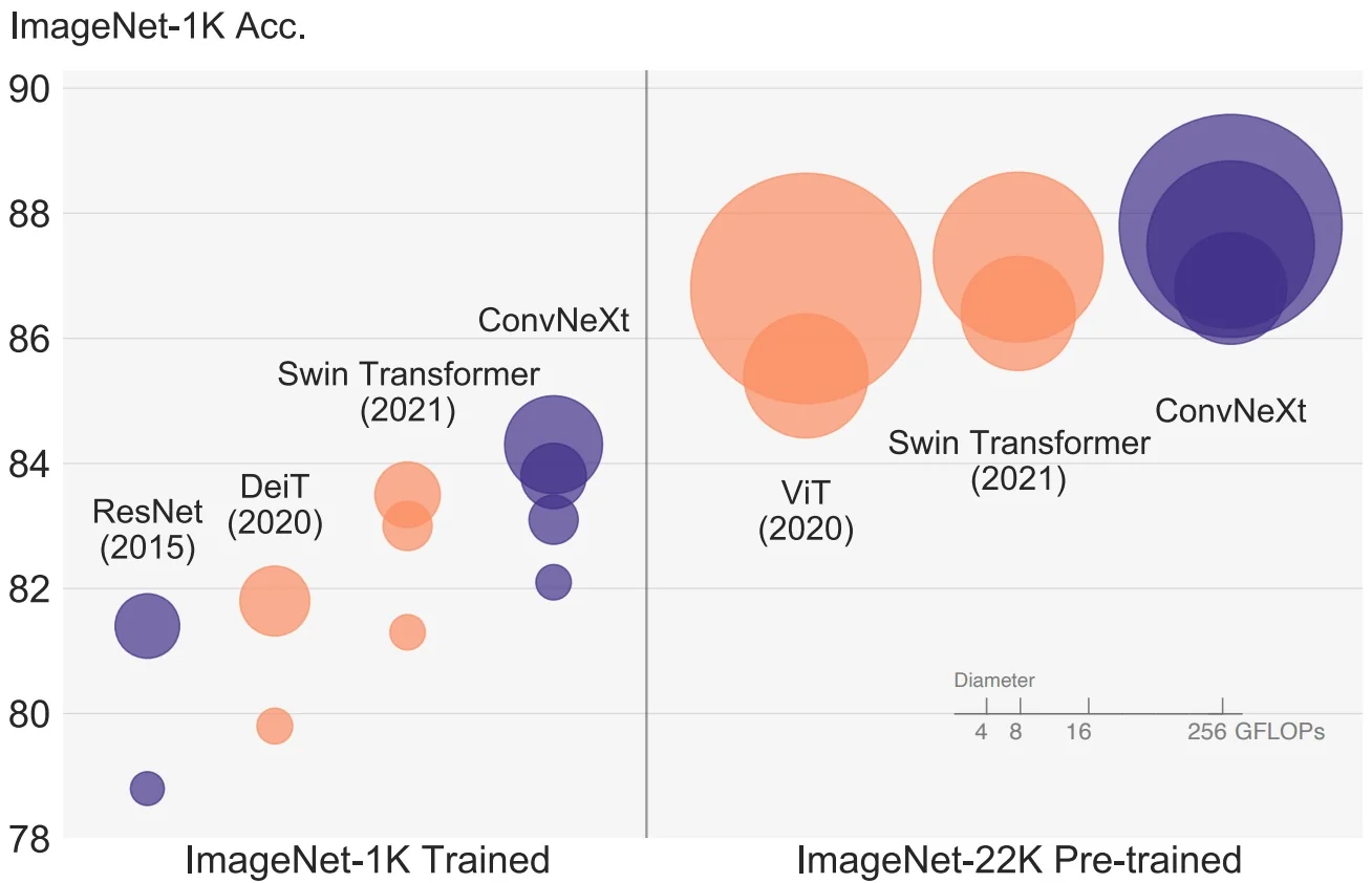
ConvNeXt: modernizing ConvNets in the ViT era ConvNeXt [400] provides a first, largely supervised answer to this scalability question. Rather than introducing a new convolution or attention operator, the authors start from a standard ResNet-50 and treat its four-stage hierarchy as a design space that can be reshaped to resemble a hierarchical Vision Transformer such as Swin. The guiding idea is pragmatic: adopt the macro- and micro-architectural patterns that appear essential in ViTs, while keeping the core computation purely convolutional.
Several concrete modifications implement this idea, each with a clear Transformer-era motivation. First, the \(7\times 7\) stride-2 stem is replaced by a single \(4\times 4\) stride-4 convolution. This operation is mathematically equivalent to forming a grid of non-overlapping \(4\times 4\) patches and projecting each patch to an embedding vector, directly mirroring the patch-embedding layer in ViTs. Subsequent downsampling between stages is performed by \(2\times 2\) stride-2 convolutions that halve the spatial resolution and increase the channel dimension, analogous to the “patch merging” layers used in Swin Transformer. In this way, ConvNeXt also operates on a hierarchy of patch-like tokens whose spatial resolution gradually shrinks while their semantic content and channel dimensionality grow.
Second, the depths of the four stages are re-balanced from the ResNet-50 pattern \((3,4,6,3)\) to \((3,3,9,3)\). These tuples record the number of residual blocks in each stage. Moving one block from the second stage into the third produces a \(1\!:\!1\!:\!3\!:\!1\) compute ratio, closely matching the “heavy third stage” pattern found in Swin (for example \((2,2,6,2)\)). This allocates more computation to the mid-resolution stage where most high-level semantics are formed, improving representational power without changing the overall FLOP budget.
Third, ConvNeXt adopts depthwise separable convolutions and an inverted bottleneck topology to decouple spatial and channel mixing, in the same spirit that Transformers separate self-attention (spatial mixing across tokens) from the MLP (channel mixing within each token). Depthwise convolutions act purely as spatial mixers on each channel, while \(1\times 1\) pointwise convolutions expand and then project back the channel dimension. To better approximate the broad spatial context of self-attention, the depthwise kernel size is later enlarged from \(3\times 3\) to \(7\times 7\), giving each block a substantially larger receptive field over the patch grid. Finally, the block micro-design is modernized by replacing BatchNorm and ReLU with LayerNorm and GELU and by using normalization and activation more sparsely, following the conventions that enable deep Transformers to train stably at scale. The resulting ConvNeXt family is still entirely convolutional, but its stage layout, patch hierarchy, and block topology now closely parallel those of modern hierarchical ViTs.
It is therefore helpful to view ConvNeXt not as a single new module, but as a modernization roadmap that gradually transforms a ResNet into a ViT-like ConvNet while staying within a similar FLOP budget. The following figure (adapted from [400]) visualizes this trajectory: early steps such as introducing depthwise convolutions reduce FLOPs, and this “saved” compute is then reinvested into wider channels and, eventually, larger kernels so that the final ConvNeXt configuration still fits in the original ResNet-50 compute envelope but achieves substantially higher ImageNet-1K and ImageNet-22K performance. This progressive trading of compute for representational capacity prepares the ground for the block-level redesign shown next, where the similarity to a Transformer layer becomes explicit.
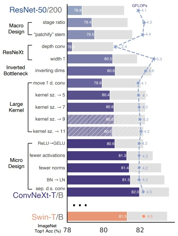
Block-level evolution and architectural convergence On the block level, ConvNeXt transitions from a ResNeXt-style bottleneck to an inverted bottleneck and finally to a block whose ordering mirrors the “spatial-then-channel” structure of a Transformer layer. The following figure (adapted from [400]) makes these intermediate steps explicit. Panel (a) shows the original ResNeXt bottleneck: a \(1\times 1\) convolution reduces channels, a \(3\times 3\) convolution performs spatial mixing, and a final \(1\times 1\) convolution restores the original channel dimension. Panel (b) introduces an inverted bottleneck: the first \(1\times 1\) convolution now expands the channels (for example, from \(96\) to \(384\)), the \(3\times 3\) depthwise convolution operates in this expanded space, and a final \(1\times 1\) convolution projects back to the narrower output. Despite increasing the FLOPs of the depthwise layer, this change reduces the overall network FLOPs by shrinking some expensive \(1\times 1\) projections in downsampling blocks, and empirically improves accuracy.
Panel (c) then reorders these components so that the depthwise \(3\times 3\) convolution is moved to the top of the block. Spatial mixing now happens before channel expansion and projection, which yields a “spatial-first, channel-second” data flow that directly parallels the attention-then-MLP structure of Transformer blocks. In the final ConvNeXt specification, this pattern is combined with larger depthwise kernels and Transformer-style normalization and activation, completing the block-level convergence.
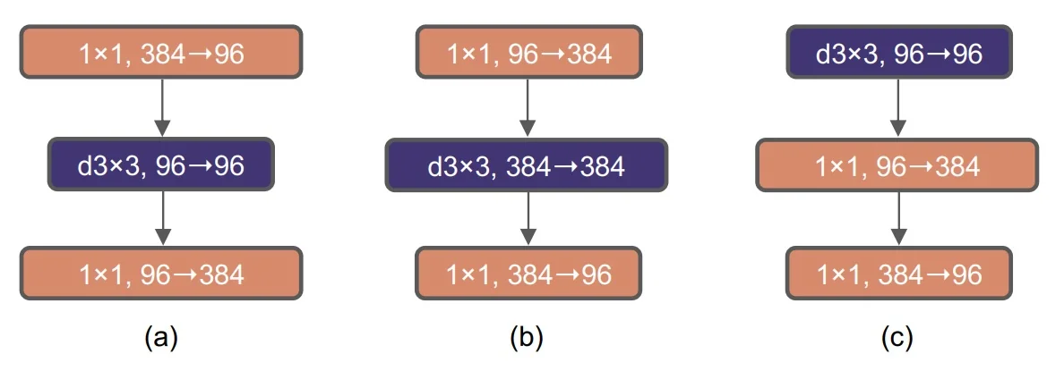
A side-by-side comparison of a ResNet bottleneck, a Swin Transformer block, and a ConvNeXt block in the next figure highlights the resulting architectural convergence. The Swin block uses window-based multi-head self-attention followed by an MLP, with LayerNorm and GELU and two residual paths per block. The final ConvNeXt block adopts the same inverted-bottleneck topology, LayerNorm+GELU micro-design, and a “spatial-first, channel-second” layout, but replaces attention windows with large-kernel (e.g. \(7\times 7\)) depthwise convolutions as the spatial mixer. In other words, the Transformer’s attention module is swapped for a convolutional spatial mixer, while the rest of the block layout is kept almost identical. This explains why ConvNeXt exhibits ViT-like scaling behavior despite being purely convolutional and retaining dense feature maps.
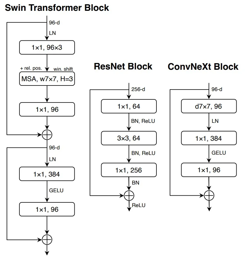
Limitations of ConvNeXt under masked autoencoding ConvNeXt was originally developed and tuned for supervised ImageNet training, where the model always sees dense images and is optimized with a cross-entropy loss on global class logits [400]. By contrast, the most effective modern pipelines for learning transferable visual representations rely on large-scale self-supervised pretraining, with Masked Autoencoders (MAE) [219] as a particularly successful example: a ViT encoder is trained to reconstruct heavily masked images and the resulting features significantly outperform purely supervised ViTs on downstream tasks. This naturally raises the question: can we plug ConvNeXt V1 into an MAE-style masked image modeling framework and obtain similar gains for ConvNets?
Woo et al. [721] show that naïvely doing so exposes two fundamental mismatches between ConvNeXt V1 and masked autoencoding. The first mismatch concerns how masking interacts with the encoder. In ViT+MAE, masking is implemented by removing patches from the token sequence: masked patches simply do not appear as tokens, so the encoder never processes the pixels it is later asked to reconstruct. The only information about a masked region that the decoder receives comes from explicit mask tokens and from context features at visible tokens.
In a convolutional encoder, we cannot remove pixels without destroying the regular grid structure, so the naïve analogue is to zero out masked pixels and run a standard dense ConvNeXt encoder. However, convolutions still operate on a full \(H\times W\) grid: a \(k\times k\) kernel centered on a masked position inevitably includes visible neighbors in its receptive field. For example, a \(3\times 3\) convolution at a masked location \((i,j)\) produces \[ y(i,j) \;=\; \sum _{u=-1}^{1} \sum _{v=-1}^{1} w_{u,v}\,I(i+u,j+v), \] where the center pixel \(I(i,j)\) is masked (zero), but several neighboring terms \(I(i+u,j+v)\) may be unmasked and non-zero. Deeper layers, whose effective receptive fields cover tens of pixels, propagate this effect: features at nominally “masked” positions become smooth interpolations of nearby visible regions. From the decoder’s perspective, the encoder has already “peeked” into masked areas via their visible neighbors, making the reconstruction task partially trivial and weakening the self-supervised signal that should force the model to learn strong long-range semantics.
The second mismatch is an optimization issue that persists even if one tries to design less leaky masking patterns. Under masked pretraining, ConvNeXt V1 exhibits a pronounced feature collapse in its expansion MLP: many channels in the \(4\times \) expansion layer become either nearly zero everywhere (dead) or uniformly large (saturated), leading to highly redundant feature maps and poor inter-channel diversity in deeper stages [721]. Empirically, MAE-style or FCMAE-style pretraining applied to the unmodified ConvNeXt V1 backbone yields only marginal improvements over strong supervised ConvNeXt baselines, in stark contrast to the clear gains observed when MAE is applied to ViT encoders. These two failures—information leakage through dense convolutions and feature collapse under masked reconstruction—motivate both a change in the pretraining framework and a modification of the ConvNeXt block itself.
ConvNeXt V2 co-designing framework and architecture ConvNeXt V2 [721] addresses these limitations through a tight co-design of training framework and backbone architecture rather than attempting to fix them with optimization tricks alone. On the framework side, a Fully Convolutional Masked Autoencoder (FCMAE) adopts a sparse-data view of masked images: visible pixels (or patch cells) are represented as active sites in a sparse tensor, and during pretraining all convolutional layers in the encoder are replaced by submanifold sparse convolutions. These convolutions compute outputs only at active sites and never activate new ones, so masked locations remain inactive throughout the encoder. In particular, there is no feature defined at a masked coordinate, and therefore no convolutional kernel centered there that could mix in neighboring visible pixels. This prevents information leakage by construction and reduces pretraining FLOPs roughly in proportion to the masking ratio, since computation is restricted to the visible \(\approx 40\%\) of spatial locations.
On the architectural side, ConvNeXt V2 inserts a Global Response Normalization (GRN) layer after the expansion MLP in every ConvNeXt block and removes the LayerScale mechanism used in ConvNeXt V1. GRN computes a global \(L_2\) energy per channel, normalizes these energies across channels, and uses the resulting scores to rescale activations, inducing strong inter-channel competition. This simple mechanism is sufficient to suppress the feature-collapse behavior observed in ConvNeXt V1 under masked pretraining and to maintain high channel diversity across depth [721].
Together, FCMAE and GRN produce a ConvNet backbone that is genuinely compatible with masked image modeling and remains stable under heavy masking. The resulting performance trend is shown in the following figure. Across a wide range of model sizes, from compact ”Atto” models designed for mobile deployment to very large ”Huge” models, self-supervised ConvNeXt V2 with FCMAE consistently outperforms both purely supervised ConvNeXt V1 and a naïve FCMAE-trained ConvNeXt V1 without GRN. This makes ConvNeXt V2 a natural starting point for modern self-supervised ConvNet backbones. The next part will examine this method in detail, following an input image through the FCMAE pipeline and then unpacking the GRN layer.
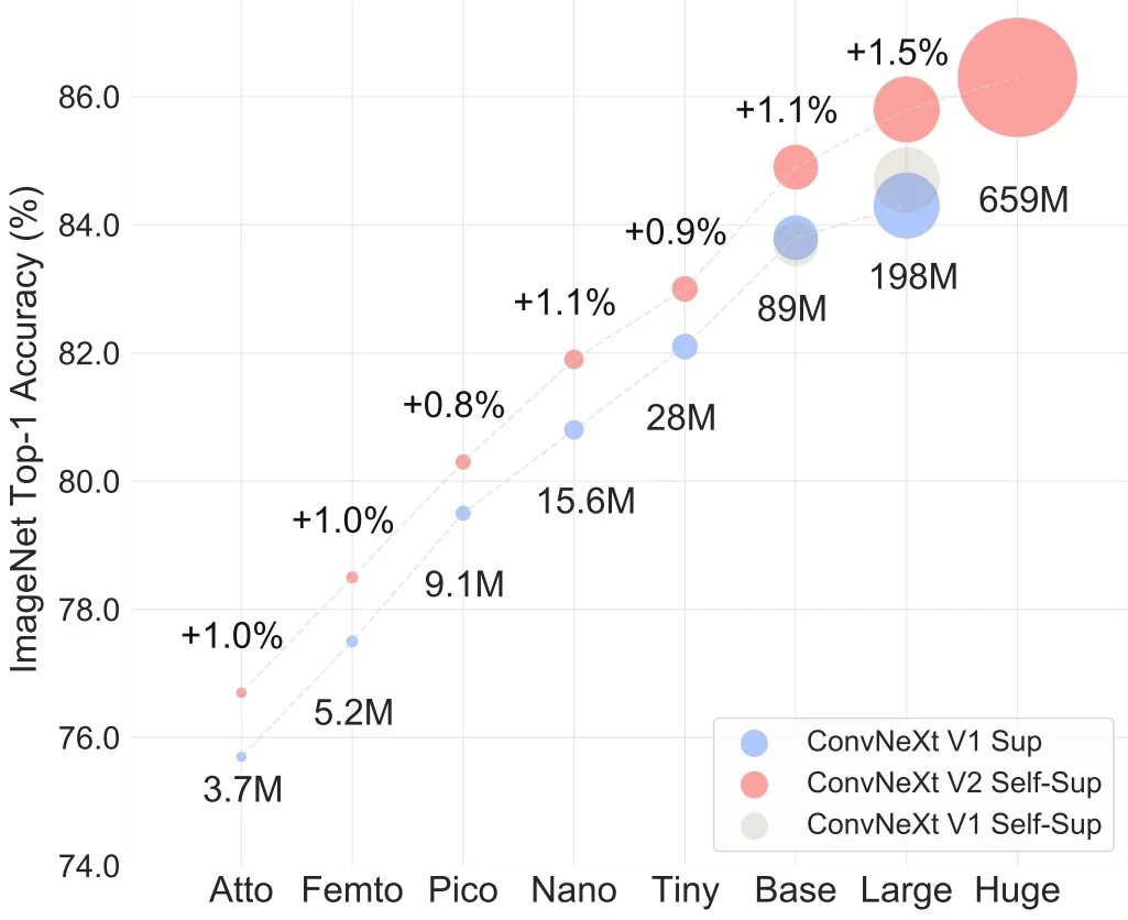
Method
High-level architecture and pretraining pipeline ConvNeXt V2 couples the ConvNeXt backbone [400] with a Fully Convolutional Masked Autoencoder (FCMAE) and Global Response Normalization (GRN) in order to make masked image modeling effective for ConvNets [721]. Architecturally, the encoder remains a four-stage ConvNeXt with a patchifying \(4\times 4\) stem, stage depths \((3,3,9,3)\), and large \(7\times 7\) depthwise convolutions in each block. What changes is the training framework: during pretraining, this ConvNeXt is embedded in an MAE-style pipeline specifically tailored to convolutions and to the leakage/feature-collapse issues identified in the previous subsection.
Given an input image \(I \in \mathbb {R}^{H \times W \times 3}\) (typically \(H=W=224\)), the FCMAE+GRN pretraining pipeline proceeds as follows:
- 1.
- Hierarchical masking. The image is partitioned into a coarse grid of patches (e.g. \(32\times 32\)). A random subset (60%) of patch indices is declared masked, and this binary mask is propagated consistently across all resolutions in the ConvNeXt hierarchy.
- 2.
- Sparse convolutional encoding. The ConvNeXt V2 encoder is run in a sparse mode: only visible (unmasked) pixels are treated as active sites, and each convolution is implemented as a submanifold sparse convolution that computes outputs exclusively at these active locations.
- 3.
- Global Response Normalization. Inside each ConvNeXt V2 block, the expansion MLP is followed by GRN, which aggregates channel energies, normalizes them across channels, and rescales activations. This induces inter-channel competition and preserves feature diversity under the masked reconstruction objective.
- 4.
- Dense decoding with mask tokens. After the sparse encoder, features are densified onto a regular grid; masked locations are filled with a learned mask token so that a lightweight ConvNeXt-style decoder can operate on a dense feature map.
- 5.
- Masked reconstruction loss. The decoder reconstructs an image \(\hat {I}\), and a mean squared error loss is computed between \(\hat {I}\) and \(I\) only over masked patches, forcing the encoder to use visible context to infer missing content.
- 6.
- Conversion to a dense ConvNeXt backbone. After pretraining, sparse convolutions are replaced by standard dense convolutions with identical kernel weights and the decoder is discarded. The resulting ConvNeXt V2 encoder is then fine-tuned under supervised objectives as a standard ConvNet backbone for classification or downstream detection/segmentation tasks.
This framework can be viewed as a convolutional analogue of MAE [219]: as in MAE, a heavy encoder, a lightweight decoder, random masking, and reconstruction on masked positions define the pretext task. However, naïvely plugging ConvNeXt V1 into the original MAE recipe breaks two key assumptions of masked autoencoding: that the encoder only sees visible patches (no information leakage) and that the learned representation remains diverse under heavy masking. FCMAE addresses the first issue by changing the encoder to operate on sparse visible sets, and GRN addresses the second by explicitly regularizing channel responses. The following paragraphs elaborate each component in more detail.
Masked image construction and hierarchical masking The FCMAE framework begins by constructing a binary mask over spatial patches. For inputs of size \(224\times 224\), the image is divided into a \(32\times 32\) grid of patches, so each patch is \(7\times 7\) pixels [721]. A random subset \(\mathcal {M}\) containing 60% of the patch indices is selected, and these patches are designated as masked, while the remaining 40% form the visible set.
ConvNeXt is hierarchical: each stage downsamples the spatial resolution by a factor of two (via \(2\times 2\) stride-2 convolutions) while increasing the channel count. To maintain a consistent notion of visibility across this pyramid, the mask is generated at the coarsest resolution (last stage) and then recursively upsampled (e.g. by nearest-neighbor or bilinear interpolation followed by thresholding) to finer stages. As a result, a spatial location is either visible at all stages or masked at all stages; there are no “partially visible” pixels that might accidentally reappear when viewed through a large receptive field.
Data augmentation during FCMAE pretraining is intentionally minimal: standard random resized cropping and horizontal flipping are used, but no strong color jitter or heavy geometric distortions. This keeps the reconstruction task well-posed and encourages the model to derive invariances primarily from the masking process rather than from aggressive augmentations.
Sparse convolutional encoder To restore the MAE assumption that the encoder should only process visible content, and at the same time to reduce computation, FCMAE reinterprets the masked image as a sparse signal and replaces all convolutions in the ConvNeXt encoder by submanifold sparse convolutions [190, 721].
During pretraining, each active spatial location corresponds to an unmasked patch (or patch cell). These active locations are stored as coordinates along with their feature vectors, forming a sparse tensor. A submanifold sparse convolution operates only on this active set: it aggregates neighbors within the kernel window but only if those neighbors are also active, and crucially it does not create new active sites at masked coordinates. Masked locations remain inactive throughout all encoder layers.
This design yields two key properties:
- Information isolation. Because masked positions are never active, no convolutional kernel is centered on them, and they never appear in any receptive field. The encoder truly only “sees” visible pixels, aligning ConvNeXt with the token-dropping semantics of ViT+MAE and eliminating the leakage described in the previous subsection.
- Computational efficiency. If 60% of patches are masked, only 40% of spatial positions remain active. Sparse convolutional layers avoid computation on masked regions, substantially reducing FLOPs and memory during pretraining compared to dense convolutions on the full grid.
After pretraining, the sparse representation is no longer needed. Each sparse convolution is replaced by a standard dense convolution with the same kernel weights, applied to dense feature maps. Since submanifold sparse convolutions and dense convolutions share the same local kernel structure on active sites, this conversion is exact: the pretrained ConvNeXt V2 encoder behaves as a standard ConvNet during fine-tuning and inference, with no additional runtime complexity beyond that of a normal ConvNeXt.
Lightweight asymmetric decoder and reconstruction loss On the decoder side, FCMAE follows the asymmetric encoder–decoder philosophy of MAE [219]: a heavy, expressive encoder and a lightweight decoder. The ConvNeXt V2 encoder is a full ConvNeXt-style backbone, whereas the decoder is a very small ConvNeXt-style network (often just a single block) with moderate channel width (e.g. 512 channels) [721].
At the interface between encoder and decoder, the sparse encoder output is densified: for each spatial location on the encoder’s output grid, unmasked positions receive their encoded feature vectors, and masked positions are filled with a learnable mask token embedding. This yields a dense feature map on which the decoder operates. The decoder then upsamples and processes this feature map to reconstruct an image \(\hat {I} \in \mathbb {R}^{H \times W \times 3}\).
Let \(\mathcal {M}\) denote the set of masked patch locations. The reconstruction objective is a mean squared error computed only on these masked patches: \[ \mathcal {L}_{\mbox{rec}} \;=\; \frac {1}{|\mathcal {M}|} \sum _{p \in \mathcal {M}} \big \| \hat {I}_p - I_p \big \|_2^2. \] Because the loss is restricted to masked regions, gradients flow primarily through the features that must infer missing content, encouraging the encoder to build context-aware representations rather than simply copying visible pixels. Ablations in Woo et al. [721] show that this minimalist decoder matches or outperforms more complex UNet- or Transformer-based decoders, while improving pretraining throughput by up to \(1.7\times \).
PyTorch-like FCMAE training step The following PyTorch-like pseudocode summarizes one FCMAE pretraining step for a ConvNeXt V2 encoder with sparse convolutions (optimizer details omitted for brevity) [721]. It implements hierarchical masking, sparse encoding, densification with mask tokens, and masked reconstruction loss.
# x: batch of images, shape (B, 3, H, W)
# convnext_sparse: ConvNeXt V2 encoder with sparse convolutions
# decoder: lightweight ConvNeXt-style decoder
# mask_generator: samples 60% random patch mask at 32x32 grid

def fcmae_step(x):
    # 1. Generate binary mask on the coarsest patch grid
    mask_coarse = mask_generator(x)           # (B, H_p, W_p), 1 = masked

    # 2. Upsample mask to full resolution
    mask_full = upsample_mask(mask_coarse, x)  # (B, 1, H, W)

    # 3. Build sparse tensor from visible pixels
    visible = (mask_full == 0)                # (B, 1, H, W)
    coords = visible.nonzero()                # (N_visible, 4) [b, c=0, h, w]
    feats = x[coords[:, 0], :,
              coords[:, 2], coords[:, 3]]    # (N_visible, 3)
    sparse_in = make_sparse_tensor(feats, coords)

    # 4. Encode visible pixels with sparse ConvNeXt V2
    z_sparse = convnext_sparse(sparse_in)     # sparse feature map

    # 5. Densify features and insert mask tokens at masked locations
    z_dense = densify_and_fill(z_sparse, mask_full)  # (B, C_enc, H’, W’)

    # 6. Decode to reconstruct image
    x_hat = decoder(z_dense)                  # (B, 3, H, W)

    # 7. Compute MSE loss on masked pixels only
    loss_mask = mask_full.expand_as(x)        # (B, 3, H, W), 1 = masked
    loss = ((x_hat - x) ** 2 * loss_mask).sum() / loss_mask.sum()
    return loss
Feature collapse under masked pretraining When ConvNeXt V1 is trained under FCMAE, Woo et al. [721] observe a severe feature collapse phenomenon even after addressing leakage via sparse encoding. In the high-dimensional expansion MLP of each block (the \(1\times 1\) convolution that increases channels by a factor of four followed by GELU), many channels become either nearly zero everywhere (dead) or uniformly large (saturated). This leads to highly redundant feature maps with little variation across channels and severely limits the expressive capacity of deeper layers.
The following figure visualizes this effect by showing 64 channel activation maps for ConvNeXt V1 vs. ConvNeXt V2 under FCMAE pretraining. ConvNeXt V1 exhibits many uniformly dark or bright channels, whereas ConvNeXt V2 with GRN produces diverse, spatially structured activations across channels.
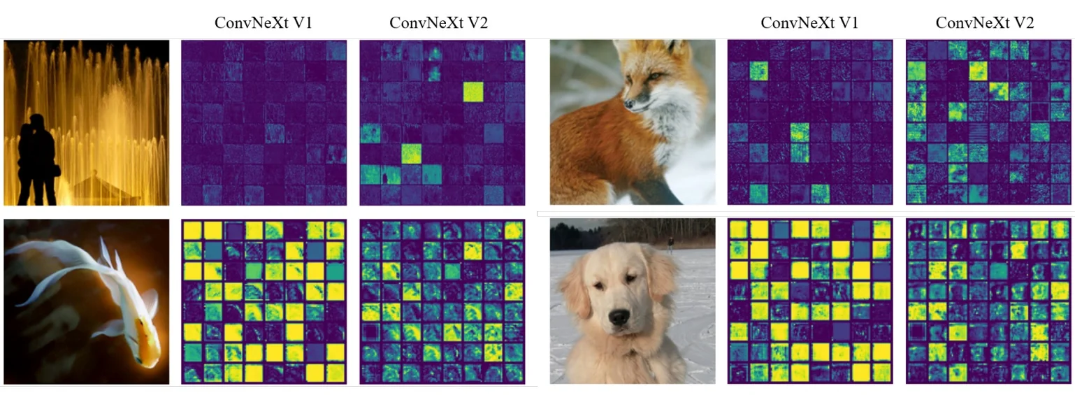
To quantify channel diversity, the authors define a layer-wise metric based on pairwise cosine distance. Given an activation tensor \(X \in \mathbb {R}^{H \times W \times C}\) and its channel-wise maps \(X_i \in \mathbb {R}^{H \times W}\), reshaped into vectors of length \(HW\), the average pairwise cosine distance is \[ d_{\mbox{cos}}(X) \;=\; \frac {1}{C^2} \sum _{i=1}^{C} \sum _{j=1}^{C} \frac {1 - \cos (X_i, X_j)}{2}. \]
High values indicate decorrelated, diverse channels; low values indicate redundancy or collapse. The below figure shows that FCMAE-trained ConvNeXt V1 exhibits a sharp drop in \(d_{\mbox{cos}}\) in deeper layers, unlike MAE-trained ViTs and FCMAE-trained ConvNeXt V2, which maintain higher diversity across depth. The supervised ConvNeXt baseline shows a modest diversity drop near the classifier head, consistent with the goal of focusing on class-discriminative features.
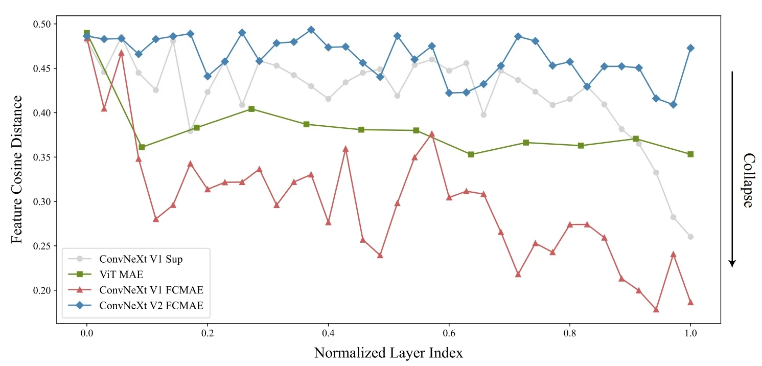
These observations motivate an architectural modification within the ConvNeXt block itself: an additional mechanism that regularizes channel responses and prevents collapse during masked pretraining.
Global Response Normalization formulation ConvNeXt V2 introduces Global Response Normalization (GRN) as a lightweight channel-wise normalization and re-weighting layer applied after the expansion MLP in each block [721]. Intuitively, GRN computes how much energy each channel contributes globally and rescales channels to encourage competition.
Given \(X \in \mathbb {R}^{H \times W \times C}\), GRN comprises three steps.
First, GRN aggregates each channel spatially using an \(L_2\) norm: \begin {equation} \mathcal {G}(X) : X \in \mathbb {R}^{H\times W\times C} \;\longrightarrow \; g_x \in \mathbb {R}^C, \label {eq:chapter11_grn_aggregation} \end {equation} where \(g_x = \{\|X_1\|_2,\dots ,\|X_C\|_2\}\) and \(X_i \in \mathbb {R}^{H \times W}\) denotes the \(i\)-th channel. The paper reports that \(L_2\)-norm aggregation performs better than global average pooling in the masked pretraining regime [721].
Second, GRN applies a divisive normalization across channels: \begin {equation} \mathcal {N}(\|X_i\|_2) \;:=\; \frac {\|X_i\|_2}{\sum _{j=1}^{C}\|X_j\|_2}. \label {eq:chapter11_grn_normalization} \end {equation} This quantity measures the relative importance of channel \(i\) compared to all others and induces a form of lateral inhibition and competition across channels, similar in spirit to classical response normalization [318].
Third, GRN calibrates the original channel features using these normalized scores: \begin {equation} \tilde {X}_i \;=\; X_i \cdot \mathcal {N}(\mathcal {G}(X)_i) \in \mathbb {R}^{H\times W}. \label {eq:chapter11_grn_calibration} \end {equation} In practice, the normalized values are also scaled by the number of channels \(C\) to account for increasing channel dimensionality in deeper layers [721]. This “core” GRN unit is parameter-free and can be implemented in a few lines of code.
Residual GRN block and PyTorch-like implementation To ease optimization and allow GRN to be gradually “turned on” during training, it is implemented with a residual connection and learnable affine parameters \(\gamma ,\beta \in \mathbb {R}^C\) initialized to zero: \[ X_i^{\mbox{out}} \;=\; \gamma \cdot \tilde {X}_i + \beta + X_i. \] With this initialization, GRN starts as an identity mapping and progressively becomes an effective normalization mechanism as \(\gamma \) and \(\beta \) deviate from zero.
The PyTorch-like pseudocode from Woo et al. [721] is reproduced below:
# Pseudocode of GRN (PyTorch-like), Woo et al. (2023).
# gamma, beta: learnable affine parameters, shape (C,).
# X: input of shape (N, H, W, C).

def grn(X, gamma, beta, eps=1e-6):
    # 1. Global L2 aggregation per channel.
    gx = torch.norm(X, p=2, dim=(1, 2), keepdim=True)  # (N, 1, 1, C)
    # 2. Divisive normalization across channels (approx. by mean).
    nx = gx / (gx.mean(dim=-1, keepdim=True) + eps)    # (N, 1, 1, C)
    # 3. Calibration with residual connection.
    return gamma * (X * nx) + beta + X
Integrating GRN into ConvNeXt blocks ConvNeXt V2 inserts GRN after the expansion MLP (\(1\times 1\) convolution that increases channels by a factor of four) and GELU, and removes the LayerScale module that ConvNeXt V1 relied on for training stability [721]. The following figure compares the ConvNeXt V1 and V2 blocks. The V2 block follows the sequence LayerNorm \(\rightarrow \) depthwise \(7\times 7\) convolution \(\rightarrow \) expansion \(1\times 1\) + GELU \(\rightarrow \) GRN \(\rightarrow \) projection \(1\times 1\), with a residual connection at the block level. Ablations show that GRN yields higher ImageNet top-1 accuracy than alternative normalization layers (LRN, BN, LN) and attention-style gating modules (SE, CBAM), while adding negligible parameters and computation [721] .
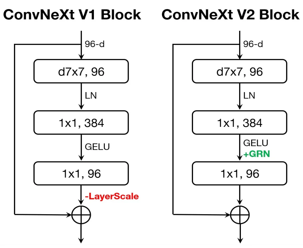
Architecture and implementation details
ConvNeXt V2 model family ConvNeXt V2 preserves the macro-architecture of ConvNeXt V1 [400, 721]. The stem performs a patchifying \(4\times 4\) convolution with stride 4, followed by four stages with depth ratios \((3,3,9,3)\) and large \(7\times 7\) depthwise convolutions in each block. The primary architectural change is the addition of GRN after the expansion MLP in every block and the removal of LayerScale. Woo et al. [721] define a model family from Atto (3.7M parameters) through Femto, Pico, Nano, Tiny, Base, Large, up to Huge (659M parameters), all sharing this ConvNeXt V2 block structure.
FCMAE pretraining and fine-tuning setup FCMAE pretraining is conducted on ImageNet-1K for 800 or 1600 epochs [721]. Inputs are resized to \(224\times 224\) or \(384\times 384\), masked at a ratio of \(0.6\), and processed by sparse ConvNeXt V2 encoders with a single ConvNeXt-block decoder of width 512. Optimization uses AdamW, cosine learning rate decay, and standard regularization (weight decay, stochastic depth), following ConvNeXt and MAE practice [400, 219]. After pretraining, sparse convolutions are converted to dense convolutions, and the ConvNeXt V2 encoder is fine-tuned on ImageNet-1K for 100 epochs under a cross-entropy loss.
ImageNet-22K intermediate fine-tuning For the largest models, ConvNeXt V2 adopts a three-stage training pipeline: FCMAE pretraining on ImageNet-1K, intermediate supervised fine-tuning on ImageNet-22K, and final supervised fine-tuning on ImageNet-1K at higher resolutions (\(384^2\) or \(512^2\)) [721]. This schedule parallels common ViT pipelines and is crucial for achieving the reported 88.9% top-1 accuracy for ConvNeXt V2-Huge while using only public data, demonstrating that a carefully co-designed self-supervised framework and architectural normalization can make ConvNets competitive with state-of-the-art ViTs at scale.
Experiments, ablations, and comparisons
Co-design of FCMAE and GRN A key set of experiments in Woo et al. [721] demonstrates that neither FCMAE nor GRN alone is sufficient; performance gains arise from their combination. For ConvNeXt-Base and ConvNeXt-Large, Table 3 reports the following.
- FCMAE on ConvNeXt V1 yields little improvement. ConvNeXt V1-Base supervised (300 epochs) achieves 83.8% top-1 accuracy; adding FCMAE pretraining without GRN yields 83.7%. ConvNeXt V1-Large improves only from 84.3% to 84.4%.
- GRN on ConvNeXt V2 under supervision yields moderate gains. ConvNeXt V2-Base supervised reaches 84.3% (+0.5% over V1-Base); ConvNeXt V2-Large supervised reaches 84.5% (+0.2%).
- Combining V2 + FCMAE yields the largest improvements. ConvNeXt V2-Base + FCMAE reaches 84.6% (+0.8% over V1-Base supervised), and ConvNeXt V2-Large + FCMAE reaches 85.6% (+1.3% over V1-Large supervised).
These results empirically support the co-design principle: the architecture and the self-supervised framework must be tuned together for masked image modeling to be effective on ConvNets.
Decoder design and pretraining efficiency Table 1 in Woo et al. [721] ablates the FCMAE decoder on ConvNeXt-Base. UNet decoders with skip connections reach 83.7% accuracy but are the slowest; removing skip connections reduces accuracy slightly to 83.5%. A Transformer-based decoder yields 83.4% but improves speed by \(1.5\times \). The single ConvNeXt-block decoder achieves 83.7% with a \(1.7\times \) speedup compared to the UNet baseline, and further ablations show that increasing decoder depth or width beyond a single \(256\)–\(512\)-channel block does not bring consistent accuracy gains.
GRN ablations Table 2 provides a detailed analysis of GRN design choices. Key findings include the following.
- Choice of aggregation. L2-norm aggregation yields 84.6% top-1 accuracy, outperforming global average pooling (83.7%) and L1-norm aggregation (84.3%).
- Normalization operator. Divisive normalization \(\|X_i\|/\sum _j \|X_j\|\) performs best (84.6%), slightly ahead of standardization \((\|X_i\|-\mu )/\sigma \) (84.5%) using the same L2-based aggregation.
- Residual connection and affine parameters. Including the residual skip and learnable affine parameters yields 84.6% vs. 84.0% without them, confirming that identity initialization helps optimization.
- Comparison to other normalizations. GRN (84.6%) surpasses LRN (83.2%), BN (80.5%), and LN (83.8%) when used in the same position within the block.
- Comparison to feature re-weighting modules. GRN (84.6%, 89M parameters) outperforms SE (84.4%, 109M) and CBAM (84.5%, 109M), providing more effective feature re-weighting without extra parameter overhead.
- Pretraining vs. fine-tuning usage. Removing GRN at fine-tuning time drops accuracy to 78.8%; adding GRN only at fine-tuning yields 80.6%. Using GRN in both pretraining and fine-tuning achieves the full 84.6% accuracy.
Masked pretraining vs contrastive learning ConvNeXt V2 also compares FCMAE to contrastive self-supervised methods such as MoCo v3 [94]. Under comparable compute budgets, FCMAE on ConvNeXt V2-Base (with 1600 epochs of pretraining) reaches around 84.9% top-1 accuracy, substantially outperforming MoCo v3 applied to ConvNeXt-style backbones (around 83.7%) [721, 94]. This suggests that, once the architecture is adapted via GRN and sparse convolutions, masked image modeling becomes a stronger pretext task than contrastive learning for ConvNets, mirroring the success of MAE for ViTs.
Comparison to transformer-based masked modeling Table 4 of Woo et al. [721] compares ConvNeXt V2 + FCMAE against BEiT, MAE on ViT, and SimMIM on Swin. At the Base scale, ConvNeXt V2-Base with FCMAE achieves higher top-1 accuracy than ViT-Base with MAE (84.9% vs. 83.6%), and at the Large scale, ConvNeXt V2-L + FCMAE slightly outperforms Swin-L with SimMIM (85.8% vs. 85.4%). In the Huge regime, ConvNeXt V2-H with ImageNet-1K-only pretraining trails ViT-H MAE by a small margin, but this gap narrows or disappears once ImageNet-22K intermediate fine-tuning is introduced.
Model scaling and state-of-the-art ImageNet accuracy Figure 11.48 illustrates that ConvNeXt V2 consistently improves upon ConvNeXt V1 across all model sizes, with the largest gains for larger models. Table 5 compares ConvNeXt V2-H (with ImageNet-22K intermediate fine-tuning) to EfficientNetV2-XL, CoAtNet-4, MaxViT-XL, MViTv2-H, and other contemporaries. ConvNeXt V2-H reaches 88.9% top-1 accuracy on ImageNet-1K at \(512^2\) resolution, setting a new state-of-the-art among models trained exclusively on public data and matching or exceeding transformer-based alternatives at similar compute [721].
Downstream detection and segmentation Tables 6 and 7 in Woo et al. [721] evaluate ConvNeXt V2 as a backbone for Mask R-CNN on COCO and UPerNet on ADE20K. Compared to ConvNeXt V1, ConvNeXt V2 supervised already improves box AP and mask AP; adding FCMAE pretraining further boosts performance. For example, ConvNeXt V2-L + FCMAE achieves 54.4 box AP and 47.7 mask AP on COCO, slightly outperforming Swin-L with SimMIM, while ConvNeXt V2-H + FCMAE reaches 55.7 box AP and 48.9 mask AP, surpassing Swin V2-H. On ADE20K, ConvNeXt V2-H + FCMAE with ImageNet-22K intermediate fine-tuning reaches 57.0 mIoU, notably higher than Swin V2-H at 54.2 mIoU. These results confirm that ConvNeXt V2 serves as a strong general-purpose backbone for dense prediction tasks, not only for classification.
Limitations and future directions
ConvNets vs transformers at extreme scales ConvNeXt V2 significantly narrows the gap between ConvNets and ViTs in the self-supervised regime, but MAE-trained ViT-H still holds a slight advantage under ImageNet-1K-only pretraining at the largest scale [219, 721]. This suggests that transformers may continue to enjoy a scaling advantage in extreme overparameterized regimes, or that additional architectural refinements (for example, richer normalization or hybrid convolution–attention modules) might be needed for ConvNets to fully match ViTs at the very top end.
Sparse convolutions and hardware support FCMAE relies on submanifold sparse convolutions for efficient processing of masked inputs during pretraining. Although an equivalent dense implementation is conceptually possible by zeroing masked locations and carefully preventing information flow across them, the theoretical efficiency benefits of FCMAE depend on actual hardware support for sparsity. On platforms without optimized sparse kernels, FCMAE may incur overhead or require specialized libraries, complicating deployment of the exact pretraining recipe. Future work may explore hardware-aware approximations that emulate the behavior of sparse convolutions using dense operations or exploit emerging accelerator support for structured sparsity.
Beyond ImageNet and pure masked modeling ConvNeXt V2 is evaluated primarily on ImageNet-1K/22K, COCO, and ADE20K, which are still relatively curated supervised datasets. It remains an open question how well FCMAE + GRN scales to more diverse, long-tailed, or multimodal data such as web-scale image–text corpora and video. Further work could investigate combinations of FCMAE with contrastive, distillation, or generative objectives, potentially requiring new architectural components co-designed for these richer training signals.
Position within modern ConvNet design philosophies Within the broader narrative of this chapter, ConvNeXt V2 is the canonical example of the modernization and scaling design philosophy for ConvNets. It demonstrates that a pure ConvNet, equipped with ViT-era macro- and micro-designs and a carefully co-designed masked autoencoding framework, can match or surpass transformer-based backbones across classification, detection, and segmentation. Subsequent enrichments will illustrate complementary philosophies: MobileNetV4 for hardware-aware unification of efficient ConvNets, and RepVGG-style architectures for training–inference decoupling via structural re-parameterization. Taken together, these perspectives form a toolkit for selecting and adapting ConvNet backbones to different deployment regimes while remaining competitive with contemporary transformers.
Enrichment 11.12.2: MobileNetV4: Universal models for the mobile ecosystem
Motivation and context
From single-device tuning to universal efficiency Early efficient ConvNets such as MobileNetV1–V3 [239, 562, 240], ShuffleNet [801], and EfficientNet [621] were typically optimized for a single deployment target, such as mobile CPUs or TPUs, often under a fixed latency or FLOP budget on that device. The design space was shaped by ideas like depthwise separable convolutions (MobileNetV1), inverted residual bottlenecks (MobileNetV2), squeeze-and-excitation (SE) channel attention [244], and compound scaling of depth, width, and resolution (EfficientNet). These models achieved impressive accuracy–efficiency trade-offs on their primary hardware, but the same architecture could be significantly suboptimal on other platforms, such as DSPs, mobile NPUs, or GPUs, due to different compute and memory characteristics. This led to a proliferation of model variants, each tuned to a specific accelerator or runtime environment rather than serving as a single universal backbone across the mobile ecosystem.
Design spaces and modern ConvNets Subsequent work shifted from one-off architectures to more systematic design spaces. RegNets [514] parameterized model families via a few global shape parameters (such as width and depth slopes), enabling controlled scaling of capacity. NFNets [54] showed that carefully designed training procedures and normalization-free blocks could push conv accuracy without BatchNorm. ConvNeXt and ConvNeXtV2 [400, 721] revisited ResNet-style ConvNets in light of Vision Transformer (ViT) [134] design, incorporating large-kernel depthwise convolutions, residual blocks that resemble transformer feed-forward networks (FFNs), and modern data augmentation and optimization recipes. The emphasis gradually moved from discovering a single best architecture to specifying a design philosophy and a flexible search space from which multiple models can be instantiated. MobileNetV4 builds directly on this trend: it treats ConvNeXt-style and inverted-bottleneck-style blocks as specific points inside a broader Universal Inverted Bottleneck (UIB) design space, and couples that space with a hardware-aware roofline objective rather than a single-device latency table.
MobileNetV4’s goal MobileNetV4 [507] targets a complementary axis in this design-space view. Rather than optimizing for one device, the authors ask how to construct a single model family that lies close to the accuracy–latency Pareto frontier on many devices simultaneously, including mobile CPUs (Pixel 6, Galaxy S23), mobile GPUs, DSPs, and dedicated accelerators such as EdgeTPU and Apple Neural Engine. The core claim is that MobileNetV4 models are “universally mostly Pareto optimal”: on a wide range of mobile and edge hardware, they achieve higher accuracy at the same latency, or lower latency at the same accuracy, compared to prior efficient ConvNets, hybrid ConvNet–Transformer models, and mobile ViT-style architectures. Put differently, MobileNetV4 aims to keep both compute units and memory pipelines well utilized on all major device classes, instead of overfitting to the quirks of a single chip.
High-level contributions To reach this goal, MobileNetV4 combines three main components.
- Roofline-guided design and analysis. The authors adopt the roofline performance model from computer architecture to reason explicitly about the interaction between computation and memory bandwidth on different devices, leading to a ridge-point-guided objective for model latency that can be evaluated analytically given per-layer MAC counts and memory traffic. By sweeping this objective over different ridge points, they effectively re-parameterize the same network under multiple compute/memory balances, making it possible to identify architectures that stay close to the Pareto frontier across heterogeneous hardware.
- Universal Inverted Bottleneck (UIB) block. MobileNetV4 introduces a flexible building block that unifies MobileNetV2-style inverted bottlenecks, ConvNeXt-style depthwise bottlenecks, extra-depthwise variants, and FFN-like pointwise-only blocks into a single super-block that can be searched per layer.
- Mobile attention and search. For hybrid models that include attention, MobileNetV4 proposes Mobile Multi-Query Attention (Mobile MQA), a memory-efficient variant of multi-head self-attention, and uses a two-stage TuNAS-style [586] neural architecture search (NAS) procedure guided by the roofline latency objective and large-scale distillation.
These ideas produce a family of MobileNetV4-Conv models (purely convolutional) and MobileNetV4 hybrid models (conv plus Mobile MQA) that collectively cover a broad Pareto front across multiple hardware platforms.
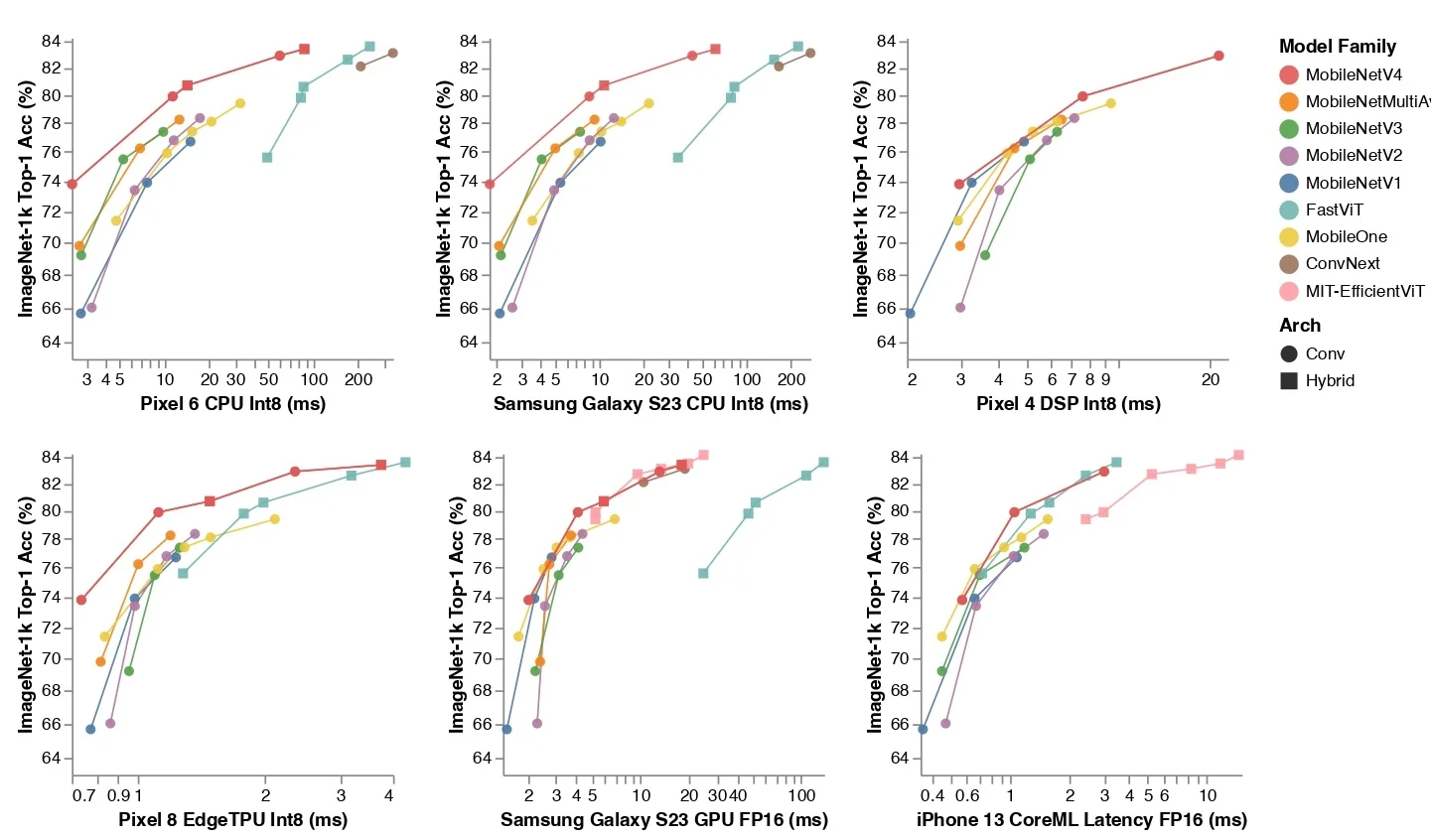
Roofline model and hardware-independent Pareto efficiency
Background: the roofline model, PeakMACs, and PeakMemBW The roofline model [718] is a standard abstraction in computer architecture for reasoning about how compute throughput and memory bandwidth jointly constrain performance. It replaces all low-level hardware details with two theoretical limits:
- PeakMACs. The maximum rate at which the processor can perform multiply–accumulate operations, measured in MAC/s. For a device with \(n_{\mbox{MAC}}\) fused multiply–add units, each capable of \(r_{\mbox{MAC}}\) MACs per cycle at a clock frequency \(f_{\mbox{clk}}\), a simple upper bound is \begin {equation} \mbox{PeakMACs} \approx n_{\mbox{MAC}} \cdot r_{\mbox{MAC}} \cdot f_{\mbox{clk}} \quad \mbox{(MAC/s)}. \end {equation}
- PeakMemBW. The maximum sustained rate at which data can be transferred between external memory and the processor, measured in bytes/s. For a memory interface with bus width \(w_{\mbox{bus}}\) bytes and effective memory clock \(f_{\mbox{mem}}\), we similarly write \begin {equation} \mbox{PeakMemBW} \approx w_{\mbox{bus}} \cdot f_{\mbox{mem}} \quad \mbox{(bytes/s)}. \end {equation}
These are device-specific constants; they do not depend on the neural network, but only on the microarchitecture (ALU count, vector width, bus width, clock frequencies).
Now consider a single neural network layer \(\ell \):
- Let \(\mathrm {MAC}_\ell \) be the total number of MACs required by that layer.
- Let \(\mathrm {Bytes}_\ell \) be the total number of bytes that must be moved to and from external memory to execute the layer (weights + activations).
Under the roofline model, the idealized time to process this layer is bounded below by two quantities: \begin {equation} t_{\mbox{comp},\ell } = \frac {\mathrm {MAC}_\ell }{\mbox{PeakMACs}}, \qquad t_{\mbox{mem},\ell } = \frac {\mathrm {Bytes}_\ell }{\mbox{PeakMemBW}}. \end {equation} Here \(t_{\mbox{comp},\ell }\) is the minimum time needed if only compute were limiting (we assume all data is instantly available), and \(t_{\mbox{mem},\ell }\) is the minimum time if only memory bandwidth were limiting (we assume compute is infinitely fast). Assuming that computation and memory accesses can be overlapped reasonably well, the layer latency is approximated by the slower of the two: \begin {equation} t_\ell = \max \left (t_{\mbox{comp},\ell }, t_{\mbox{mem},\ell }\right ). \end {equation}
A key quantity in this framework is the operational intensity (sometimes called arithmetic intensity) of the layer: \begin {equation} \mbox{OI}_\ell = \frac {\mathrm {MAC}_\ell }{\mathrm {Bytes}_\ell } \quad \mbox{(MACs/byte)}. \end {equation} This measures how many MACs are performed per byte of data transferred from memory.
The ridge point (RP) of a device is defined as the ratio between its peak compute throughput and peak memory bandwidth: \begin {equation} \mbox{RP} = \frac {\mbox{PeakMACs}}{\mbox{PeakMemBW}} \quad \mbox{(MACs/byte)}. \end {equation}
In the MobileNetV4 paper, RP is interpreted as the minimum operational intensity required to achieve maximum computational performance: layers with \(\mbox{OI}_\ell < \mbox{RP}\) cannot saturate compute because they are limited by memory bandwidth, whereas layers with \(\mbox{OI}_\ell \ge \mbox{RP}\) are compute-limited [507]. Combining the definitions above, we can write \begin {equation} t_{\mbox{comp},\ell } = \frac {\mathrm {MAC}_\ell }{\mbox{PeakMACs}} = \frac {\mathrm {Bytes}_\ell \cdot \mbox{OI}_\ell }{\mbox{PeakMACs}} = \frac {\mathrm {Bytes}_\ell }{\mbox{PeakMemBW}} \cdot \frac {\mbox{OI}_\ell }{\mbox{RP}} = t_{\mbox{mem},\ell } \cdot \frac {\mbox{OI}_\ell }{\mbox{RP}}. \end {equation} The equality \(t_{\mbox{comp},\ell } = t_{\mbox{mem},\ell }\) occurs exactly when \(\mbox{OI}_\ell = \mbox{RP}\); this is the ridge of the roofline. Thus:
- If \(\mbox{OI}_\ell < \mbox{RP}\), then \(t_{\mbox{comp},\ell } < t_{\mbox{mem},\ell }\) and the layer is memory-bound: latency is dominated by data movement.
- If \(\mbox{OI}_\ell > \mbox{RP}\), then \(t_{\mbox{comp},\ell } > t_{\mbox{mem},\ell }\) and the layer is compute-bound: latency is dominated by arithmetic throughput.
Low-RP devices (typical for general-purpose CPUs) have relatively weak peak compute compared to memory bandwidth, so many layers end up compute-bound. High-RP devices (typical for accelerators and NPUs) have very strong compute arrays but limited external bandwidth, so many layers become memory-bound unless their operational intensity is high.
From layer-level roofline to the MobileNetV4 latency objective MobileNetV4 turns this layer-wise roofline model into an analytic latency predictor for an entire network, which is then used directly as a differentiable objective in its architecture search. For a network with layers \(\ell = 1,\dots ,L\), the predicted model time for a device characterized by \((\mbox{PeakMACs}, \mbox{PeakMemBW})\) is \begin {equation} \mbox{ModelTime}(\mbox{RP}) = \sum _{\ell =1}^{L} t_\ell = \sum _{\ell =1}^{L} \max \left ( \frac {\mathrm {MAC}_\ell }{\mbox{PeakMACs}}, \frac {\mathrm {Bytes}_\ell }{\mbox{PeakMemBW}} \right ). \label {eq:chapter11_mobilenetv4_modeltime} \end {equation} This is exactly the form of Equation (1) in the MobileNetV4 paper, written in terms of \(\mathrm {MAC}_\ell \) and \(\mathrm {Bytes}_\ell \). In practice:
- \(\mathrm {MAC}_\ell \). For a convolutional layer, \(\mathrm {MAC}_\ell \) is computed from the output spatial resolution, input and output channel counts, kernel area, and group size (for depthwise or group convolutions). For fully connected layers, it is simply the product of input and output dimensions.
- \(\mathrm {Bytes}_\ell \). MobileNetV4 models \(\mathrm {Bytes}_\ell \) as the sum of weight bytes and activation bytes. Weight bytes depend on kernel shape, channel counts, and numerical precision (e.g., float32 or int8). Activation bytes depend on the feature map spatial size, channels, and precision.
It is often convenient to factor out the memory term using the operational intensity: \begin {align} t_\ell &= \max \left ( \frac {\mathrm {MAC}_\ell }{\text {PeakMACs}}, \frac {\mathrm {Bytes}_\ell }{\text {PeakMemBW}} \right ) = \frac {\mathrm {Bytes}_\ell }{\text {PeakMemBW}} \max \left ( \frac {\text {OI}_\ell }{\text {RP}}, 1 \right ). \end {align}
Thus, up to the global scaling factor \(1/\mbox{PeakMemBW}\), the relative ordering of network latencies is fully determined by \begin {equation} \sum _{\ell =1}^{L} \mathrm {Bytes}_\ell \cdot \max \left (\frac {\mbox{OI}_\ell }{\mbox{RP}},\,1\right ), \end {equation} which depends on the hardware only through the single scalar \(\mbox{RP} = \mbox{PeakMACs}/\mbox{PeakMemBW}\).
If we scale both \(\mbox{PeakMACs}\) and \(\mbox{PeakMemBW}\) by the same constant, RP is unchanged and all model times are rescaled by the same factor; the Pareto ordering between architectures is identical. In other words, the roofline model collapses the full hardware description into a one-dimensional parameter RP.
MobileNetV4 exploits this property in two ways:
- Hardware-independent ranking. Because \(\mbox{ModelTime}(\mbox{RP})\) depends on hardware only through RP, any two devices with the same ridge point will rank networks in the same order of predicted latency. The same analytic objective can therefore be used to design models that are competitive on many present and future devices whose RPs fall in a given range.
- Ridge point sweep. The paper evaluates \(\mbox{ModelTime}(\mbox{RP})\) for RP values swept from \(0\) to \(500\) MACs/byte, spanning regimes from “MAC-only” (RP \(=0\), equivalent to optimizing purely for total MAC count) through CPU-like RPs (a few to a few tens of MACs/byte) up to accelerator-like RPs (hundreds of MACs/byte). For each RP, they can draw an accuracy–latency Pareto frontier and check whether a candidate architecture remains near-optimal across the entire sweep.
The resulting picture is that the ridge point RP re-parameterizes the latency objective: by varying a single scalar, the same formula interpolates smoothly between compute-bound and memory-bound hardware.
MobileNetV4 uses this roofline-based \(\mbox{ModelTime}(\mbox{RP})\) both to reason analytically about where different operations (Conv2D, depthwise convolutions, fully connected layers) are expensive, and to select architectures whose predicted latency remains competitive across a wide range of RPs, yielding hardware-independent (or “universal”) Pareto efficiency.
Ridge-point sweep and its interpretation To understand how different architectures behave across the mobile ecosystem, the authors sweep RP over a range of values:
- RP = 0. A limiting case corresponding to a roofline model with effectively infinite memory bandwidth (“MACs-only”): \(\mbox{MemTime}_\ell = 0\) for all layers, so models are ordered purely by their total MACs [507]. This recovers the common practice of using MAC count as a latency proxy.
- RP \(\in [5, 50]\). A range that roughly matches the “Slow CPU” (RP \(= 5\)) and “Fast CPU” (RP \(= 50\)) settings in the following figure. At such low ridge points, hardware is typically compute-bound: reducing MACs directly reduces latency, even if this slightly increases memory traffic. Models optimized for this regime behave like classic “MAC-minimizing” MobileNets.
- RP \(\approx 500\). A regime corresponding to accelerator-like devices (DSPs, EdgeTPUs) where data movement is the bottleneck. Here layers with low operational intensity (depthwise convolutions, fully connected layers) become memory-bound and dominate latency, whereas dense Conv2D layers with high operational intensity can add model capacity at little additional latency cost.
For each network and each RP, MobileNetV4 evaluates Equation (11.21) to obtain a predicted latency, then plots ImageNet-1k accuracy versus this model time. The result is a family of accuracy–latency trade-off curves parameterized by RP. When an architecture remains near the upper-left Pareto frontier across a broad RP range, it is predicted to be universally efficient across both CPU-like and accelerator-like devices and to maintain high utilization of both compute and memory resources.
The quantity \(1/\mbox{RP}\) can be interpreted as the number of bytes that can be moved per MAC at the ridge point (bytes per MAC), but in practice the RP sweep is performed directly in MACs/byte space. The absolute scale of PeakMACs and PeakMemBW cancels out when comparing architectures; only their ratio (RP) affects the relative ordering of networks.
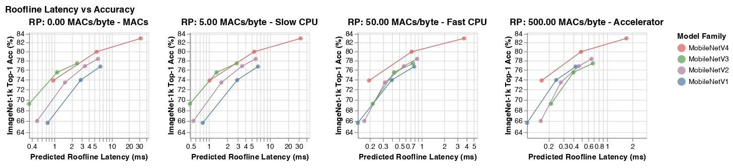
Operation types across devices To gain more intuition, the authors decompose the roofline latency into contributions from different operation types (standard convolutions, depthwise convolutions, fully connected layers) across the network. For each layer \(\ell \) and operation type \(o\), the latency contribution is given by the same max formula as Equation (11.21), and these contributions are plotted along the depth of the network for different ridge points.
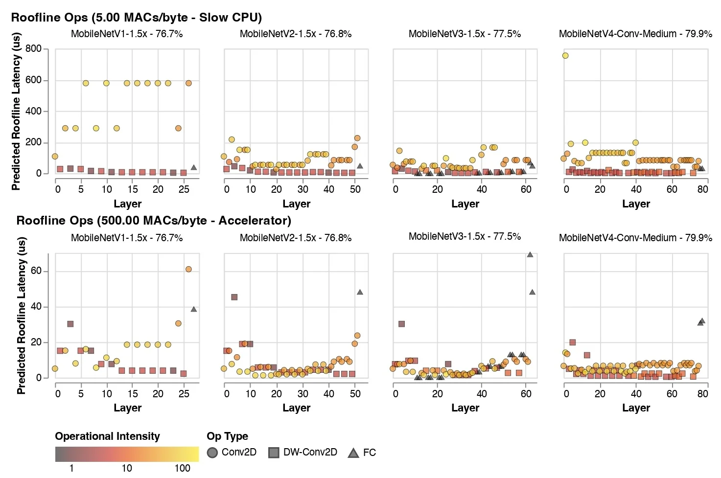
These plots reveal a characteristic pattern that matches the discussion in [507]. On low-RP hardware (CPU-like), large Conv2D layers are expensive because their MAC count dominates latency: when compute is the bottleneck, high-intensity operations with many MACs per byte (dense convolutions) are slow, whereas low-MAC operations such as depthwise Conv2D and fully connected layers are comparatively cheap. On high-RP hardware (accelerator-like), the situation reverses: MACs are abundant, but external memory bandwidth is tight, so low-intensity operations (depthwise and FC layers) become memory-bound and dominate latency, while dense Conv2Ds with high operational intensity add capacity at little additional latency cost.
MobileNetV4 responds by structuring the architecture so that MAC-intensive Conv2D layers are concentrated near the beginning of the network and memory-intensive fully connected layers occur near the end. This layout avoids having both dense Conv2Ds and FC layers as simultaneous worst-case bottlenecks on any single hardware class. Depthwise convolutions appear primarily in intermediate stages, where they provide spatial mixing at low MAC cost, and the NAS-controlled UIB variants modulate how heavily they are used at different resolutions. This arrangement is consistent with the layer-wise roofline plots in Figure 11.54 and helps explain why MobileNetV4 remains near the Pareto frontier across ridge points (Figures 11.52 and 11.53).
Universal Inverted Bottleneck (UIB) block
Recap: inverted bottlenecks, ConvNeXt blocks, and FFNs MobileNetV2 introduced the inverted residual bottleneck (MBConv) [562], where a narrow input is first expanded with a \(1\times 1\) convolution, then processed by a depthwise convolution, and finally projected back to a narrow output with another \(1\times 1\) convolution. This design leverages cheap depthwise convolutions to provide spatial mixing, while pointwise convolutions carry most of the channel mixing.
MobileNetV3 [240] augmented MBConv with squeeze-and-excitation and nonlinearities such as hard-swish.
ConvNeXt [400] proposed a different block structure, closer to a transformer feed-forward block: a depthwise convolution with a relatively large kernel (e.g., \(7\times 7\)) followed by a channel-wise MLP implemented as two pointwise convolutions with a nonlinearity and normalization in between. In parallel, ViT-style FFNs apply two linear layers with a nonlinear activation and residual connection [664, 134]. From a high-level perspective, MBConv, ConvNeXt blocks, and FFNs share similar ingredients (depthwise or spatial mixing plus channel-wise MLPs) but arrange them differently.
UIB as a unifying super-block Neural architecture search (NAS) is most effective when the search space balances expressivity with hardware pragmatism. If the space is too restrictive, NAS merely rediscovers known patterns; if it is too unconstrained, it may generate architectures that are theoretically efficient (low MACs) but perform poorly on real devices due to unsupported operators, fragmented kernels, or operations with very low operational intensity on accelerators.
MobileNetV4 addresses this by introducing the Universal Inverted Bottleneck (UIB) super-block: a single, carefully curated template that unifies the most successful micro-architectural patterns from MobileNetV2/V3, ConvNeXt, and ViT-like FFNs, while restricting itself to operations that are well supported across mobile CPUs, GPUs, DSPs, and NPUs.
Conceptually, the UIB consists of:
- Input expansion. A pointwise (\(1\times 1\)) convolution that expands channels from \(C_{\mbox{in}}\) to \(C_{\mbox{mid}}\).
- Two optional depthwise convolutions. One depthwise layer that can be placed before expansion (a “start” depthwise convolution) and one depthwise layer that can be placed after expansion but before projection (a “middle” depthwise convolution).
- Output projection. A pointwise (\(1\times 1\)) convolution that projects from \(C_{\mbox{mid}}\) back to \(C_{\mbox{out}}\).
By toggling the two depthwise layers on or off, the same template can instantiate extra-depthwise, MobileNet inverted bottleneck, ConvNeXt-like, and FFN-like blocks, covering the main families of efficient ConvNet and ViT-style micro-architectures within a single design.
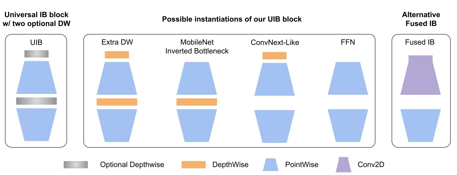
UIB parameterization and curated search space The UIB is therefore not a single fixed block but a compact search space parameterized by a small number of discrete and continuous choices:
- Channel widths. The expansion ratio \(r = C_{\mbox{mid}} / C_{\mbox{in}}\) and the output width \(C_{\mbox{out}}\).
- Depthwise presence and kernel sizes. Binary switches for the two depthwise convolutions (enabled or disabled) and their kernel sizes (typically \(3\times 3\), \(5\times 5\), or \(7\times 7\)).
- Fused vs. non-fused. A flag indicating whether to realize the expansion-plus-depthwise pattern as separate layers or as a single fused \(k\times k\) Conv2D (Fused-IB).
This search space is deliberately curated: it is restricted to operators with mature, optimized support in mobile inference libraries (Conv2D, depthwise Conv2D, and fully connected/pointwise layers). The UIB explicitly avoids more fragile or less portable building blocks (e.g., exotic activations, dynamic-shape operations, early attention, or irregular tensor layouts) that often cause deployment or performance issues on edge accelerators. In this way, NAS retains enough freedom to discover new layer compositions, but every sampled architecture is “deployment-safe” by construction.
UIB variants and roofline behavior Each UIB instantiation occupies a distinct region in the roofline space from Section 11.12.2.0, trading off MAC count, bytes moved, and thus operational intensity \(\mbox{OI}_\ell = \mathrm {MAC}_\ell / \mathrm {Bytes}_\ell \) in different ways:
- Extra-depthwise (StartDW + MiddleDW). Structure: Both depthwise convolutions are enabled around expansion, yielding two depthwise layers plus expansion and projection. Role: Provides strong spatial mixing and rapid receptive-field growth at low MAC cost. Roofline behavior: Attractive on low-RP, compute-limited devices (CPUs), but the two low-intensity depthwise steps can become memory-bound on high-RP accelerators.
-
MobileNet inverted bottleneck (MiddleDW only). Structure: Only the post-expansion depthwise convolution is enabled, yielding the classic MBConv pattern (expansion \(\rightarrow \) depthwise \(\rightarrow \) projection) with optional squeeze-and-excitation, as in MobileNetV2/V3. Role: Balances channel capacity (via expansion) and spatial context (via a single depthwise layer).
Roofline behavior: The depthwise layer has low operational intensity, while the two pointwise layers are high-intensity; overall this behaves well across moderate ridge points and serves as a robust default backbone pattern.
- ConvNeXt-like (StartDW only). Structure: Only the pre-expansion depthwise convolution is enabled, performing spatial mixing at width \(C_{\mbox{in}}\) followed by a pointwise MLP (expansion and projection). Role: Allows cheaper spatial mixing on a narrower tensor, often enabling larger kernels (\(5\times 5\) or \(7\times 7\)) while keeping the block Conv2D- and depthwise-friendly. Roofline behavior: Shifts some cost from dense pointwise layers to a depthwise layer at lower channel width; suitable when large-kernel depthwise convolutions are well-optimized and memory bandwidth can sustain the initial activation reads.
- FFN-like (no depthwise). Structure: Both depthwise convolutions are disabled, leaving only expansion and projection pointwise layers, matching a ViT-style FFN with channel-wise mixing and no spatial mixing inside the block. Role: Maximizes arithmetic intensity and channel capacity while relying on other blocks or stages for spatial context. Roofline behavior: Nearly all cost is in dense \(1\times 1\) convolutions, yielding very high operational intensity; this is ideal for high-RP accelerators that prefer heavy arithmetic over additional memory traffic.
Because every block in MobileNetV4 is a UIB, NAS can allocate these variants according to the ridge point regime:
- On CPU-like hardware (low RP), depthwise-heavy variants (extra-depthwise or MobileNet inverted bottleneck) can dominate early and mid stages, achieving good accuracy at low MAC budgets where compute is scarce but memory bandwidth is relatively less constraining.
- On accelerator-like hardware (high RP), FFN-like and fused variants with higher operational intensity can be preferred, especially in stages where feature maps are large and memory-bound depthwise operations would otherwise dominate latency.
The small set of UIB toggles therefore implicitly spans a range of operational intensities, and the NAS controller chooses, per layer, which side of the roofline (compute- vs. memory-bound) to operate on for a given ridge point.
Fused inverted bottleneck The fused inverted bottleneck (Fused-IB) is a hardware-driven specialization of the UIB for high-RP devices. In a standard MBConv-like UIB, expansion and depthwise convolution are separate operations: the expanded feature map is written to memory after the \(1\times 1\) expansion and then read back for the depthwise convolution, incurring additional memory traffic.
In Fused-IB, these two steps are replaced by a single dense \(k\times k\) Conv2D that both expands channels and performs spatial mixing in one kernel, followed by the usual \(1\times 1\) projection. From a purely MAC-count perspective this is more expensive, but it significantly increases operational intensity: more arithmetic is performed per byte loaded, and intermediate activations do not need to be materialized in external memory. On accelerators with very high \(\mbox{PeakMACs}\) relative to \(\mbox{PeakMemBW}\) (large RP), this trade-off is beneficial: the extra MACs are “cheap” compared to the savings in memory traffic.
MobileNetV4 therefore uses Fused-IB primarily in early, high-resolution stages (the stem and early blocks), where feature maps are largest and roofline analysis indicates that memory traffic, not compute, is the dominant bottleneck. Later stages, where spatial resolutions are smaller and depthwise operations become less memory-intensive, can revert to non-fused MBConv-like or ConvNeXt-like UIBs, giving NAS fine-grained control over the operational intensity profile across depth.
UIB pseudo-code The following pseudo-code illustrates a simplified UIB block in PyTorch-like notation, showing how optional depthwise convolutions and fused variants can be configured.
class UIBlock(nn.Module):


def __init__(self, C_in, C_mid, C_out,
             use_dw1=False, k_dw1=3,
             use_dw2=False, k_dw2=3,
             fused=False, act=nn.SiLU()):
    super().__init__()
    self.fused = fused

    if fused:
        # Fused-IB: kxk Conv2D replaces StartDW + expansion.
        self.conv_fused = nn.Conv2d(
            C_in, C_mid, kernel_size=k_dw1,
            stride=1, padding=k_dw1 // 2,
            groups=1, bias=False)
        # No separate depthwise layers in the fused case.
        self.dw1 = None
        self.dw2 = None
    else:
        # Optional depthwise before expansion ("StartDW").
        self.dw1 = nn.Conv2d(
            C_in, C_in, kernel_size=k_dw1,
            stride=1, padding=k_dw1 // 2,
            groups=C_in, bias=False) if use_dw1 else None

        # Pointwise expansion to C_mid.
        self.expand = nn.Conv2d(
            C_in, C_mid, kernel_size=1, bias=False)

        # Optional depthwise after expansion ("MiddleDW").
        self.dw2 = nn.Conv2d(
            C_mid, C_mid, kernel_size=k_dw2,
            stride=1, padding=k_dw2 // 2,
            groups=C_mid, bias=False) if use_dw2 else None

    # Final projection from C_mid to C_out (shared across variants).
    self.project = nn.Conv2d(
        C_mid, C_out, kernel_size=1, bias=False)

    self.act = act


def forward(self, x):
    identity = x

    if self.fused:
        # Single fused Conv2D does spatial mixing + expansion.
        x = self.act(self.conv_fused(x))
    else:
        # Optional pre-expansion depthwise.
        if self.dw1 is not None:
            x = self.act(self.dw1(x))
        # Expansion.
        x = self.act(self.expand(x))
        # Optional post-expansion depthwise.
        if self.dw2 is not None:
            x = self.act(self.dw2(x))

    # Projection is always applied.
    x = self.project(x)

    # Residual connection (when shapes match).
    if x.shape == identity.shape:
        x = x + identity

    return x
MobileNetV4 uses a parametrized version of this super-block within a NAS framework, allowing the search algorithm to enable or disable depthwise convolutions and to select their kernel sizes per block and per stage. During search, the UIB behaves like a re-parameterizable template: many block variants share a common description, while the final exported model for inference is a standard ConvNet composed of a concrete subset of these variants.
Mobile MQA attention for hybrid models
Background: MHSA and its limitations on mobile hardware Hybrid ConvNet–Transformer architectures often incorporate multi-head self-attention (MHSA) to model long-range dependencies. Given queries \(Q \in \mathbb {R}^{L \times d}\), keys \(K \in \mathbb {R}^{L \times d}\), and values \(V \in \mathbb {R}^{L \times d}\), MHSA for \(H\) heads typically computes \begin {equation} \mbox{MHSA}(Q, K, V) = \mbox{Concat}\left (\mbox{head}_1, \dots , \mbox{head}_H\right ) W^O, \end {equation} where each head uses distinct projections \(W^Q_h, W^K_h, W^V_h\) and computes \begin {equation} \mbox{head}_h = \mbox{Softmax}\left (\frac {Q W^Q_h (K W^K_h)^\top }{\sqrt {d_h}}\right ) V W^V_h. \end {equation} This design is flexible but expensive on mobile hardware for two reasons:
- Memory intensity. Multiple key and value projections require storing and moving separate \(K_h\) and \(V_h\) tensors per head, stressing bandwidth.
- Quadratic cost in sequence length. The attention matrix has shape \(L \times L\), and even modest increases in token count can significantly increase computation and memory.
Multi-query attention Multi-Query Attention (MQA) [581] was introduced in language models to address some of these issues. MQA keeps multiple query projections but shares a single set of keys and values across heads: \begin {equation} K' = X W^K, \quad V' = X W^V, \quad Q_h = X W^Q_h, \end {equation} where \(X\) is the input sequence. Each head then computes \begin {equation} \mbox{head}_h = \mbox{Softmax}\left (\frac {Q_h K'^\top }{\sqrt {d_h}}\right ) V'. \end {equation} This reduces memory and compute for the key and value paths while preserving the per-head flexibility in queries. The MobileNetV4 paper emphasizes that one shared head for keys and values greatly reduces memory access when the number of tokens is relatively small compared to the feature dimension, which is exactly the regime of late-stage hybrid vision models on mobile devices [507].
Mobile MQA design MobileNetV4 introduces a Mobile MQA block tailored to vision and mobile hardware. The core ideas are:
- Shared keys and values across heads. As in standard MQA, a single \(K'\) and \(V'\) are computed per block and shared by all query heads, significantly reducing memory traffic and parameter count in the key/value projections.
- Asymmetric spatial reduction. Drawing on Spatial Reduction Attention (SRA), Mobile MQA optionally downsamples only the key/value path with a stride-2 depthwise convolution, while retaining full-resolution queries. This creates an asymmetric compute profile: attention is computed over a shorter \(K'/V'\) sequence, reducing quadratic cost and memory accesses, but the output still has the original spatial resolution.
- Conv-friendly implementation and einsum layout. Projections and downsampling are implemented with Conv2D and depthwise Conv2D operations that map well to mobile accelerators. The attention core is implemented as a single einsum/GEMM with tensor layouts chosen so that contracted and non-contracted indices are contiguous in memory, avoiding expensive intermediate transposes and reshapes.
In the MobileNetV4 experiments, replacing MHSA with Mobile MQA in a MNv4-Conv-L backbone yields over \(39\%\) speedup on EdgeTPU and Samsung S23 GPU, while also reducing MACs and parameters by more than \(25\%\) with negligible accuracy change [507].
For a feature map \(X \in \mathbb {R}^{B \times C \times H \times W}\), a simplified Mobile MQA block can be written as:
class MobileMQA(nn.Module):


def __init__(self, C, num_heads, reduction=2):
    super().__init__()
    self.num_heads = num_heads
    self.d_kv = d_kv       # shared KV dimension
    self.reduction = reduction

    # Per-head queries at full resolution.
    self.q_proj = nn.Conv2d(C, C, kernel_size=1, bias=False)

    # Shared keys and values at reduced resolution (single KV head).
    self.kv_proj = nn.Conv2d(C, 2 * d_kv, kernel_size=1, bias=False)

    # Depthwise downsampling for spatial reduction on K/V only.
    self.dw_down = nn.Conv2d(
        C, C, kernel_size=3, stride=reduction,
        padding=1, groups=C, bias=False
    )

    self.out_proj = nn.Conv2d(C, C, kernel_size=1, bias=False)


def forward(self, x):
    B, C, H, W = x.shape

    # Shared K and V at reduced resolution.
    x_down = self.dw_down(x) if self.reduction > 1 else x   # B, C, H’, W’
    kv = self.kv_proj(x_down)                               # B, 2*d_kv, H’, W’
    K, V = kv.chunk(2, dim=1)                               # B, d_kv, H’, W’

    # Queries at full resolution.
    Q = self.q_proj(x)                                      # B, C, H, W

    # Flatten spatial dimensions.
    Q = Q.flatten(2).transpose(1, 2)    # B, L, C
    K = K.flatten(2).transpose(1, 2)    # B, L_kv, d_kv
    V = V.flatten(2).transpose(1, 2)    # B, L_kv, d_kv

    # Reshape queries into heads; keys/values stay shared (single KV head).
    d_head = C // self.num_heads
    Q = Q.view(B, -1, self.num_heads, d_head)    # B, L, H, d_head
    Q = Q.permute(0, 2, 1, 3)                    # B, H, L, d_head

    # Attention with shared K/V (broadcast over heads).
    # Layout chosen so contracted and non-contracted indices are contiguous.
    K_t = K.transpose(1, 2)                      # B, d_kv, L_kv
    scores = torch.einsum("bhld,bdm->bhlm", Q, K_t) / math.sqrt(d_head)
    attn = scores.softmax(dim=-1)                # B, H, L, L_kv

    out = torch.einsum("bhlm,blm->bhld", attn, V)  # B, H, L, d_head

    # Merge heads and project back to (B, C, H, W).
    out = out.permute(0, 2, 1, 3).contiguous()
    out = out.view(B, -1, C)  # B, L, C
    out = out.transpose(1, 2).view(B, C, H, W)
    out = self.out_proj(out)
    return out
This code highlights the two Mobile MQA-specific design choices:
-
Only a single, shared key/value projection is computed (dimension \(d_{kv}\)), which is broadcast across all heads; this is the defining property of MQA and is what reduces memory traffic relative to MHSA.
- Asymmetric spatial down-sampling is applied to \(K\) and \(V\) but not to \(Q\), so attention operates over a shorter sequence while preserving the input and output resolution. This directly improves operational intensity on high-RP accelerators by reducing memory-bound work in the K/V path.
In the official implementation, the einsum formulation is further tuned so that the contracted and non-contracted dimensions align with the underlying GEMM layout used by the hardware kernels, eliminating the need for explicit tensor transposes and contributing to the reported \(\sim 39\%\) speedup of Mobile MQA over MHSA on EdgeTPU and mobile GPUs.
NAS recipe and model construction
Design principles for the search space MobileNetV4’s NAS formulation is built around three principles:
- Standard operations only. The search space is restricted to Conv2D, depthwise Conv2D, and fully connected layers (and Mobile MQA for hybrid models), all of which are well supported and quantization friendly on mobile hardware.
- Flexible UIB block per layer. Each block in the network is a UIB super-block whose specific instantiation (MBConv-like, ConvNeXt-like, FFN-like, extra-depthwise, fused) is chosen by NAS, along with kernel sizes and expansion ratios.
- Roofline-guided latency objective. The NAS objective combines ImageNet-1k accuracy (via distillation) with the roofline-predicted ModelTime at representative ridge points for the target hardware.
This design lets the search algorithm reason about the trade-off between accuracy and latency across a broad range of devices while keeping the space implementable and deployable.
Two-stage TuNAS-style search The authors use a TuNAS-style differentiable NAS framework [586] with a two-stage search strategy designed to mitigate a known bias in weight-sharing SuperNets. In a shared-parameter SuperNet, candidates with fewer parameters (e.g., smaller kernels or lower expansion factors) tend to converge faster and therefore appear stronger early in training, which biases the search policy toward them even when larger kernels would be better at convergence [507].
To address this, MobileNetV4 decouples macro-architecture design from fine-grained kernel and depthwise choices:
- Stage 1: coarse-grained filter search. At this stage, the search focuses on global architectural parameters such as per-stage widths (channel counts) and depths (number of blocks), under a fixed UIB configuration (e.g., an inverted bottleneck with expansion factor 4 and a \(3\times 3\) depthwise kernel). The goal is to identify a good backbone shape that yields strong accuracy under distillation while keeping roofline-predicted latency low on representative ridge points.
- Stage 2: fine-grained depthwise and kernel search. With the coarse backbone fixed, the search space is refined to include depthwise presence and kernel sizes inside UIB blocks. The search now considers the placement of the two optional depthwise convolutions and their kernel sizes (typically \(3\times 3\) or \(5\times 5\)), allowing the model to adjust spatial mixing and operational intensity per layer to optimize latency across ridge points.
Empirically, the two-stage search improves both accuracy and latency compared to a one-stage baseline. For a fixed target latency on EdgeTPU, the two-stage strategy improves ImageNet-1k top-1 accuracy by roughly \(0.2\%\) and reduces latency by almost \(5\%\) relative to a one-stage TuNAS search.
Teacher models and distillation To stabilize NAS and achieve strong final accuracy, architectures are trained and evaluated via distillation from a large, high-accuracy teacher. MobileNetV4 uses an EfficientNet-L2 teacher [621] trained on JFT-300M with a modern training recipe. For each candidate architecture, the student is trained on a mixture of datasets:
- Augmented ImageNet replicas. ImageNet-1k variants with strong data augmentation (including mixup and RandAugment), providing diverse views of the base dataset.
- Extreme mixup. Distributions created by aggressive mixing of multiple images and labels, encouraging robustness and smoothing of the decision boundary.
- Class-balanced JFT subset. A subset of JFT-300M constructed to balance rare and common classes, improving coverage of underrepresented visual concepts.
This “dynamic dataset mixing” is used during both the NAS phase and the final model training, and ablations in the paper show that including the class-balanced JFT subset yields significant improvements in student accuracy at modest additional training cost.
Final model extraction Once the NAS procedure converges, the controller chooses a single architecture (or a small set of architectures) for each target model size. These architectures are then retrained from scratch (or with distillation) using a strong training recipe:
- Long training. Hundreds to thousands of epochs on mixed datasets with learning rate schedules similar to those used in contemporary ConvNet work (cosine decay, warmup).
- Strong regularization and augmentation. Label smoothing, mixup, stochastic depth, and adaptive gradient clipping, aligned with best practices from NFNets and EfficientNet.
- Quantization-aware deployment. Training and calibration procedures that allow models to be deployed efficiently with low-precision arithmetic on mobile platforms.
The resulting architectures form the MobileNetV4-Conv and MobileNetV4-Hybrid families described in the next subsubsection.
Importantly, all NAS machinery disappears at inference time: the deployed models are plain ConvNets (plus attention in hybrid variants) built from standard primitives, so the NAS process can be viewed as a training-time re-parameterization of the design space into a single fixed architecture that is well matched to many devices.
Architecture and implementation details
Stage-wise structure MobileNetV4 models follow the familiar four-stage backbone pattern used by prior MobileNets and EfficientNets. For an input of size \(224 \times 224\), the spatial resolution is progressively reduced by strided convolutions or depthwise convolutions, while channel counts increase:
- Stem. A fused inverted bottleneck or standard Conv2D with stride 2 to quickly reduce resolution while keeping early features conv-friendly for all hardware.
- Low-level stages. One or two stages at \(112 \times 112\) and \(56 \times 56\) resolution using mainly fused UIB blocks, emphasizing dense Conv2D operations that are efficient on accelerators and acceptable on CPUs.
-
Mid-level stages. Intermediate stages at \(28 \times 28\) or \(14 \times 14\) resolution that mix MBConv-like and ConvNeXt-like UIBs, chosen by NAS to provide a balance between depthwise and dense convolutions depending on the target hardware.
- High-level stages. Final stages at \(14 \times 14\) and \(7 \times 7\) resolution that may include FFN-like UIBs and, in hybrid models, Mobile MQA blocks to capture long-range dependencies with reduced spatial resolution.
The exact number of blocks per stage, expansion ratios, and kernel sizes differ across models (S, M, L, hybrid variants), but all are drawn from the UIB search space with roofline-guided choices.
Purely convolutional vs. hybrid models MobileNetV4-Conv models use only convolutional UIB and fused UIB blocks. They achieve strong accuracy–latency trade-offs across devices and are particularly attractive when attention-friendly kernels are not available or when minimal runtime complexity is desired.
MobileNetV4-Hybrid models insert Mobile MQA blocks into higher stages to enhance global representation capacity. The number and placement of Mobile MQA blocks is part of the search space and is chosen jointly with UIB configurations. On devices with strong attention kernels (e.g., some NPUs), these hybrid models can provide additional accuracy gains at competitive latency, especially on tasks that benefit from long-range modeling.
Training and implementation notes Training details follow modern ConvNet practice:
- Data augmentation. RandAugment, mixup, CutMix, and random erasing are used to improve robustness and prevent overfitting.
- Optimization. Optimizers such as RMSProp or AdamW with cosine learning rate decay, warmup, and EMA of weights are used, tuned per model size.
- Regularization. Label smoothing, stochastic depth, and drop-path are employed, with drop-path rates scaled by depth.
The paper emphasizes that training recipes for MobileNetV1–V3 baselines were also upgraded to match these modern practices, ensuring that comparisons against MobileNetV4 reflect architectural improvements rather than outdated training.
Experiments and ablations
ImageNet classification and universal Pareto optimality On ImageNet-1k, MobileNetV4-Conv and MobileNetV4-Hybrid models achieve state-of-the-art accuracy–latency trade-offs across multiple hardware platforms. For example:
- MobileNetV4-Conv-S. Achieves roughly \(73.8\%\) top-1 accuracy with about \(2.4\) ms latency on a Pixel 6 CPU, running about twice as fast as MobileNetV3 at similar accuracy.
- MobileNetV4-Conv-M. Provides a mid-sized backbone that is more than \(50\%\) faster than MobileOne-S4 on EdgeTPU at comparable accuracy, and substantially faster than MobileNetV2 while being more accurate.
- MobileNetV4-Hybrid-L. Achieves close to \(87\%\) ImageNet-1k top-1 accuracy while running in about \(3.8\) ms on a Pixel 8 EdgeTPU, with far fewer parameters and MACs than the EfficientNet-L2 teacher.
Across CPUs, GPUs, DSPs, and NPUs, most MobileNetV4 variants lie on or very close to the empirical accuracy–latency Pareto frontier, as shown in Figure 11.52. Competing models such as FastViT, EfficientViT, and various mobile ViTs may excel on one device but fall behind on others, whereas MobileNetV4 is consistently competitive.
Ablations on UIB search space The paper includes a set of ablations where the NAS is restricted to narrower search spaces:
- IB-only search. When the search space is restricted to MBConv-like blocks, top-1 accuracy drops and MACs must be increased to compensate, leading to worse Pareto trade-offs.
- ConvNeXt-only search. When only ConvNeXt-like depthwise-plus-MLP blocks are allowed, accuracy remains competitive but latency increases on some devices, especially those where depthwise convolutions are memory-bound.
- Full UIB search. Allowing all UIB instantiations yields the best accuracy at similar or lower predicted latency across ridge points, confirming that per-layer flexibility is beneficial for universal efficiency.
These results support the interpretation of UIB as a genuinely useful unifying abstraction rather than a cosmetic combination of existing blocks.
Ablations on Mobile MQA Mobile MQA ablations compare:
- MHSA vs. MQA. Replacing standard MHSA with Mobile MQA on a fixed backbone reduces EdgeTPU latency by around \(39\%\) and shrinks parameter count and MACs by over \(25\%\), with negligible impact on ImageNet accuracy.
- Effect of spatial reduction. Adding stride-2 depthwise downsampling to Mobile MQA yields approximately \(23\%\) MAC reduction and \(25\%\) CPU speedup for attention blocks, with small accuracy loss, demonstrating the benefits of reducing sequence length.
- Kernel and head variations. Varying kernel sizes and head counts produces expected trade-offs between expressivity and efficiency; the MobileNetV4 choices represent a balanced point in this space.
NAS and distillation ablations NAS ablations show that the two-stage TuNAS strategy improves the accuracy–latency trade-off compared to a single-stage search, confirming the benefit of decoupling coarse backbone design from fine-grained depthwise configuration. Distillation ablations demonstrate that:
- Dynamic dataset mixing. Mixing augmented ImageNet replicas with extreme mixup improves student accuracy relative to using either alone.
- Adding a class-balanced JFT subset. Incorporating a class-balanced subset of JFT-300M further boosts accuracy, especially for larger models like MobileNetV4-Conv-L.
- Extended training. Extending student training to around \(2000\) epochs enables MobileNetV4-Conv-L to reach approximately \(85.9\%\) top-1 accuracy, within about \(1.6\%\) of its EfficientNet-L2 teacher despite being much smaller and cheaper.
Object detection and transfer Beyond classification, the authors evaluate MobileNetV4 backbones in RetinaNet-style object detection on COCO. A MobileNetV4-Conv-M backbone achieves roughly \(32.6\%\) AP while being faster on Pixel 6 CPU than MobileNetV2 and MobileNetMultiAvg backbones, and a MobileNetV4-Hybrid-M backbone improves AP to around \(34.0\%\) with an \(18\%\) CPU latency penalty. These results highlight MobileNetV4’s suitability as a general-purpose backbone for on-device detection and segmentation in addition to classification.
Limitations and future directions
Limitations of the roofline model The roofline-based latency objective relies on simplified assumptions about compute and memory behavior. It ignores:
- Cache hierarchies and tiling. Real devices may reuse data in caches more effectively than the simple \(\mathrm {Bytes}_\ell \) model suggests, or suffer from bank conflicts and other microarchitectural effects that the model does not capture.
- Kernel scheduling and fusion. Vendor libraries often fuse operations (e.g., convolution plus activation plus normalization), altering effective MAC and memory costs relative to the idealized model.
- Non-Conv2D operations and software effects. Operations such as reshapes, concatenations, specialized attention kernels, pruning, or quantization may have costs that are not accurately captured by the MACs-and-bytes abstraction. As the paper itself notes, techniques with complex memory access patterns (such as some forms of pruning) can appear much better on a roofline model than on actual hardware, because software implementation overheads are abstracted away.
Despite these limitations, the strong correlation between analytical predictions and actual on-device latency in Figure 11.52 and Figure 11.53 suggests that the roofline model is sufficiently accurate to guide architectural design, but practitioners should still benchmark final models on target hardware and batch sizes.
Dependence on large-scale distillation MobileNetV4 leverages an EfficientNet-L2 teacher trained on JFT-300M with a sophisticated recipe. Reproducing this pipeline requires access to large proprietary datasets and significant training compute. While the student models are efficient and deployable, their quality depends on the existence of a strong teacher. Future work could explore:
- Teacher-free NAS. Using self-supervised pretraining or training-from-scratch objectives that do not rely on massive labeled datasets.
- Open-source teachers. Building comparable pipelines using publicly available datasets such as ImageNet-21k or LAION-style web corpora.
Search space and hardware evolution The UIB search space is tailored to today’s mobile hardware and supports Conv2D, depthwise Conv2D, and Mobile MQA. As hardware evolves (e.g., with improved sparse tensor support, new attention primitives, or 3D convolution accelerators), this search space may need to be revisited. Future directions include:
- Incorporating sparsity and low-rank structure. Extending the UIB space to include structured sparsity or low-rank approximations that are natively supported by emerging accelerators.
- Multi-objective search. Beyond accuracy and latency, integrating energy consumption, memory footprint, and quantization robustness into the NAS objective.
Summary and connections to other architectures Within the broader narrative of the chapter, MobileNetV4 exemplifies the hardware-aware unification philosophy. ConvNeXt and ConvNeXtV2 demonstrate how modernized ConvNets can compete with ViTs as general-purpose backbones, while RepVGG and related re-parameterization methods illustrate training–inference decoupling for simple inference graphs. MobileNetV4 complements these by showing how a carefully chosen super-block (UIB), combined with a roofline-guided latency model that is re-parameterized by the ridge point RP and a TuNAS-style NAS, can yield a single family of models that is near-optimal across diverse hardware platforms. In practical terms, MobileNetV4 provides a concrete recipe for building depthwise-separable ConvNets that remain competitive across CPUs, GPUs, DSPs, and NPUs, and it offers a natural reference point for subsequent sections on efficient architectures, re-parameterization techniques, and mobile deployment.
Enrichment 11.12.3: RepVGG Making VGG-style ConvNets Great Again
RepVGG [129] is a modern example of training–inference decoupling for ConvNets, designed to reconcile three trends discussed throughout this chapter. First, residual and multi-branch architectures such as ResNet and ResNeXt [215, 730] improved optimization and accuracy by making networks behave like implicit ensembles. Second, channel-attention and scaling families such as Squeeze-and-Excitation (SE) [244], EfficientNet [621], RegNet [514], and ConvNeXt/ConvNeXtV2 [400, 721] pursued better accuracy–FLOP trade-offs through sophisticated macro-designs and search. Third, hardware- and platform-aware families such as MobileNetV1/V2/V3 [239, 562, 240], ShuffleNet [801, 420], and more recently MobileNetV4 [507] focus on roofline-guided design and depthwise separable operators for mobile and edge deployment, while large-scale families such as NFNets [54] primarily target high-throughput training on datacenter accelerators rather than strict mobile efficiency. RepVGG takes a different path. It keeps the inference-time network as simple as a VGG-style stack of \(3\times 3\) convolutions and ReLUs, while using a multi-branch residual-like topology only during training and then collapsing it by structural re-parameterization. [129].
Motivation
From VGG simplicity to multi-branch complexity The starting point for RepVGG is the contrast between early ConvNets and modern architectures. VGG [592] popularized a simple “single-path” template composed of a stack of \(3\times 3\) convolutions, ReLUs, and pooling, and achieved strong ImageNet performance with a relatively straightforward design. Subsequent architectures such as Inception, ResNet, DenseNet, and ResNeXt [617, 215, 253, 730] shifted attention toward increasingly elaborate multi-branch topologies, skip connections, and dense feature reuse to improve optimization and accuracy, at the cost of more complicated computation graphs and operator mixes.
Hardware efficiency issues in modern ConvNets More recent families such as Xception and MobileNets [106, 239, 562] heavily rely on depthwise separable convolutions; ShuffleNet [801, 420] adds channel shuffle operations; Squeeze-and-Excitation [244] introduces per-channel attention; and EfficientNet [621] and RegNet [514] use compound scaling or design spaces to find good accuracy–FLOP Pareto fronts. These designs are attractive in terms of theoretical FLOPs, but they combine many small operators, nontrivial data movement, and less mature library support. In practice, architectures with lower nominal FLOPs can be slower than simpler models with much higher FLOPs on the same GPU, because FLOPs ignore both memory access cost and achievable parallelism [129]: in roofline terms, many depthwise- or multi-branch-heavy designs operate in a memory-bound regime (low arithmetic intensity), whereas a dense stack of large \(3\times 3\) convolutions tends to be compute-bound and can saturate the peak throughput of cuDNN-style Winograd kernels. A concrete example highlighted in the RepVGG paper is that VGG-16 has roughly \(8.4\times \) the FLOPs of EfficientNet-B3, yet VGG-16 runs about \(1.8\times \) faster on a single 1080Ti GPU [129]. This discrepancy arises because:
- Memory access cost dominates. Multi-branch and depthwise-heavy designs often move data between many small tensors, increasing memory traffic relative to useful computation.
- Parallelism is fragmented. Architectures produced by NAS or with heterogeneous operators may have many small kernels that underutilize GPU cores, whereas large, regular \(3\times 3\) convolutions can fully exploit Winograd implementations and SIMD units.
This hardware perspective motivates revisiting plain, VGG-style ConvNets that use a single operator type and a simple feed-forward dataflow.
Plain ConvNets are attractive but hard to train Plain ConvNets without residual branches are attractive for deployment. A feed-forward topology with a single operator type allows:
- High computational density. A stack of stride-1 \(3\times 3\) convolutions can fully exploit Winograd implementations: with the standard \(F(2\times 2, 3\times 3)\) algorithm, the number of multiplications drops to \(4/9\) of a direct \(3\times 3\) conv, so each layer achieves much higher effective TFLOPS per FLOP than mixtures of kernel sizes or depthwise operators [129].
- Memory efficiency. In a plain network, feature maps can be freed as soon as the next layer is computed, lowering peak activation memory relative to multi-branch networks that must buffer branch inputs until addition or concatenation.
- Architectural flexibility. Without shortcut constraints, layer widths and depths can be tuned or channel-pruned layer-by-layer, without worrying about matching shapes across branches or maintaining residual connections.
However, attempts to train deep plain ConvNets have historically suffered from optimization difficulties and inferior accuracy compared to residual networks, even when using careful initialization, BatchNorm, and other stabilizing tricks [636, 129]. Residual networks can be interpreted as implicit ensembles of many shallower paths [665], which improves gradient flow and optimization; plain networks lose this benefit.
Structural re-parameterization as the missing piece RepVGG observes that the advantages of multi-branch architectures are largely training-time phenomena: branches provide easier optimization and better representational flexibility during training, but are undesirable at inference because they reduce parallelism, increase memory footprint, and complicate hardware. At the same time, plain \(3\times 3\)-only architectures are highly desirable at inference but difficult to optimize from scratch. Existing re-parameterization methods such as DiracNet [771] express a convolution kernel as a combination of an identity term and a learned residual kernel, but they modify the parameterization rather than the network structure and still underperform ResNets. Component-level structural re-parameterizations such as ACNet [128] focus on kernel-level improvements and can be dropped into arbitrary architectures, but they do not by themselves solve the problem of training deep plain ConvNets. RepVGG therefore proposes to explicitly decouple training and inference: use a ResNet-inspired multi-branch block during training for optimization, then algebraically collapse the block into a single \(3\times 3\) convolution for inference, yielding a VGG-style stack of identical \(3\times 3\)-ReLU layers.
Method: Structural re-parameterization for VGG-style ConvNets
Training-time RepVGG block The basic building block of RepVGG during training is a three-branch structure inspired by ResNet but designed to be exactly convertible into a single \(3\times 3\) convolution [129]. Given an input feature map \(M^{(1)} \in \mathbb {R}^{N \times C_1 \times H \times W}\), a RepVGG block with matching input and output dimensions (\(C_1 = C_2\), stride \(1\)) consists of:
- A \(3\times 3\) convolution branch. A convolution with kernel \(W^{(3)} \in \mathbb {R}^{C_2 \times C_1 \times 3 \times 3}\) followed by BatchNorm with parameters \((\mu ^{(3)}, \sigma ^{(3)}, \gamma ^{(3)}, \beta ^{(3)})\).
- A \(1\times 1\) convolution branch. A convolution with kernel \(W^{(1)} \in \mathbb {R}^{C_2 \times C_1}\) (viewed as \(C_2 \times C_1 \times 1 \times 1\)) followed by its own BatchNorm with parameters \((\mu ^{(1)}, \sigma ^{(1)}, \gamma ^{(1)}, \beta ^{(1)})\).
- An identity branch. If the spatial and channel dimensions match, the input is forwarded through an identity operation followed by BatchNorm with parameters \((\mu ^{(0)}, \sigma ^{(0)}, \gamma ^{(0)}, \beta ^{(0)})\); if dimensions differ (e.g., stride-2 or channel increase), this branch is omitted.
Let \(bn(\cdot ;\mu ,\sigma ,\gamma ,\beta )\) denote the inference-mode BatchNorm. The pre-activation output \(M^{(2)}\in \mathbb {R}^{N\times C_2\times H\times W}\) of a block with all three branches can be written as \begin {equation} \label {eq:repvgg_block_training} \begin {aligned} M^{(2)} = &\; bn\big (M^{(1)} * W^{(3)};\mu ^{(3)},\sigma ^{(3)},\gamma ^{(3)},\beta ^{(3)}\big ) \\ &+ bn\big (M^{(1)} * W^{(1)};\mu ^{(1)},\sigma ^{(1)},\gamma ^{(1)},\beta ^{(1)}\big ) \\ &+ bn\big (M^{(1)};\mu ^{(0)},\sigma ^{(0)},\gamma ^{(0)},\beta ^{(0)}\big ), \end {aligned} \end {equation} followed by a single ReLU nonlinearity. The identity branch makes the block behave like a residual block \(y = x + f(x)\), while the additional \(1\times 1\) branch increases representational capacity and the effective ensemble size during training. Crucially, there are no nonlinearities (e.g., ReLU) inside individual branches; the only nonlinearity is applied after summation, which is essential for exact re-parameterization.
Plain inference-time block After training, the goal is to convert each multi-branch block into a single \(3\times 3\) convolution with kernel \(\widetilde {W} \in \mathbb {R}^{C_2\times C_1\times 3\times 3}\) and bias \(\widetilde {b}\in \mathbb {R}^{C_2}\) such that for any input \(M^{(1)}\), \begin {equation} \label {eq:repvgg_equiv} M^{(2)} = \widetilde {M}^{(2)} = \widetilde {M}^{(1)} * \widetilde {W} + \widetilde {b}, \end {equation} where \(\widetilde {M}^{(1)} = M^{(1)}\), and the same ReLU is applied afterward. This equivalence is achieved in three algebraic steps:
- 1.
- Fuse each convolution and its following BatchNorm into a single convolution with bias.
- 2.
- Rewrite the identity branch as a \(1\times 1\) convolution with an identity kernel, then fuse it with its BatchNorm as well.
- 3.
- Embed each \(1\times 1\) kernel into a \(3\times 3\) kernel by zero-padding and add all resulting \(3\times 3\) kernels and biases elementwise.
This procedure realizes the structural re-parameterization illustrated later in the re-parameterization figure.
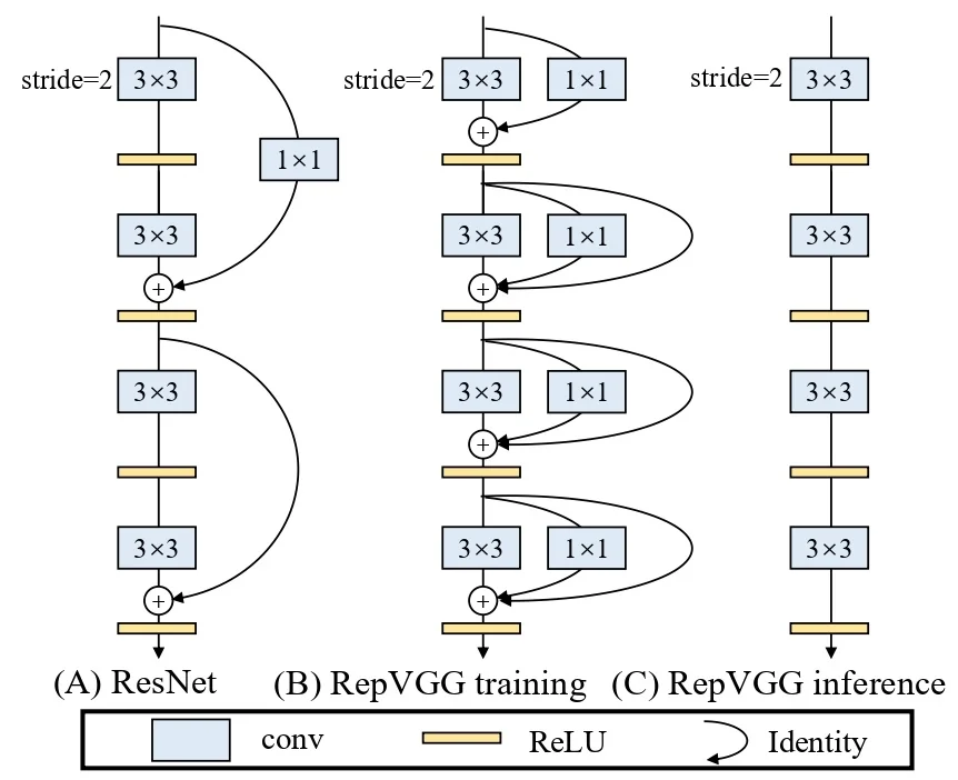
BatchNorm fusion Consider a generic convolution followed by BatchNorm. Let \(W \in \mathbb {R}^{C_2 \times C_1 \times k \times k}\) be the kernel (without bias), and \((\mu ,\sigma ,\gamma ,\beta )\) the BatchNorm running mean, standard deviation, scale, and shift. For an intermediate feature map \(M\), inference-mode BatchNorm acts channelwise as \begin {equation} \label {eq:repvgg_bn} bn(M;\mu ,\sigma ,\gamma ,\beta )_{n,i,h,w} = \frac {\gamma _i}{\sigma _i}\big (M_{n,i,h,w} - \mu _i\big ) + \beta _i, \end {equation} for each output channel \(i\in \{1,\dots ,C_2\}\). If \(M = M^{(1)} * W\), then this composition can be rewritten as a convolution with kernel \(W_0\) and bias \(b_0\) defined by \begin {equation} \label {eq:repvgg_bn_fuse} W_{0,i,:,:,:} = \frac {\gamma _i}{\sigma _i} W_{i,:,:,:}, \qquad b_{0,i} = -\frac {\mu _i\gamma _i}{\sigma _i} + \beta _i. \end {equation} Substituting into (11.29) gives \begin {equation} \label {eq:repvgg_bn_fuse_equiv} bn(M^{(1)} * W;\mu ,\sigma ,\gamma ,\beta )_{:,i,:,:} = (M^{(1)} * W_0)_{:,i,:,:} + b_{0,i}. \end {equation} This fusion transformation is applied independently to each branch before they are summed: to the \(3\times 3\) branch, the \(1\times 1\) branch, and the identity branch (treated as a \(1\times 1\) convolution whose kernel is the channelwise identity matrix).
Rewriting identity and \(1\times 1\) convolutions as \(3\times 3\) After BatchNorm fusion, each branch is represented by a kernel and a bias:
- A fused \(3\times 3\) kernel. A kernel \(W^{(3)}_0 \in \mathbb {R}^{C_2\times C_1 \times 3 \times 3}\) with bias \(b^{(3)}_0\).
- A fused \(1\times 1\) kernel. A kernel \(W^{(1)}_0 \in \mathbb {R}^{C_2\times C_1 \times 1 \times 1}\) with bias \(b^{(1)}_0\).
- A fused identity kernel. A kernel \(W^{(0)}_0 \in \mathbb {R}^{C_2\times C_1 \times 1 \times 1}\) with bias \(b^{(0)}_0\), where \(W^{(0)}_0\) is an identity matrix over channels (when the branch is present).
To sum the branches at the level of convolution parameters, the kernels must share the same spatial support. RepVGG achieves this by embedding each \(1\times 1\) kernel into the central element of a \(3\times 3\) kernel and zero-padding elsewhere. Define padded kernels \begin {equation} \label {eq:repvgg_pad} \widehat {W}^{(1)}_{0,i,j,:,:} = \begin {cases} W^{(1)}_{0,i,j,1,1}, & (u,v) = (1,1), \\ 0, & \mbox{otherwise}, \end {cases} \quad \widehat {W}^{(0)}_{0,i,j,:,:} = \begin {cases} W^{(0)}_{0,i,j,1,1}, & (u,v) = (1,1), \\ 0, & \mbox{otherwise}, \end {cases} \end {equation} for spatial indices \((u,v)\in \{0,1,2\}^2\) (with center index \((1,1)\)). The \(3\times 3\) kernel already has the desired shape and is left unchanged.
Summing kernels and biases Because convolution is linear in both the kernel and the input, summing the three branch outputs is equivalent to convolving with the sum of the kernels and adding the sum of the biases. Hence the final equivalent kernel \(\widetilde {W}\) and bias \(\widetilde {b}\) are \begin {equation} \label {eq:repvgg_final_kernel} \widetilde {W} = W^{(3)}_0 + \widehat {W}^{(1)}_0 + \widehat {W}^{(0)}_0, \qquad \widetilde {b} = b^{(3)}_0 + b^{(1)}_0 + b^{(0)}_0. \end {equation} Substituting into (11.28) and comparing with (11.27) shows that, under the assumptions that all branches share the same stride and that the \(1\times 1\) branches use one pixel less padding than the \(3\times 3\) branch, the single \(3\times 3\) convolution with parameters \((\widetilde {W},\widetilde {b})\) is exactly equivalent to the three-branch structure followed by summation. This is the essence of structural re-parameterization used by RepVGG.
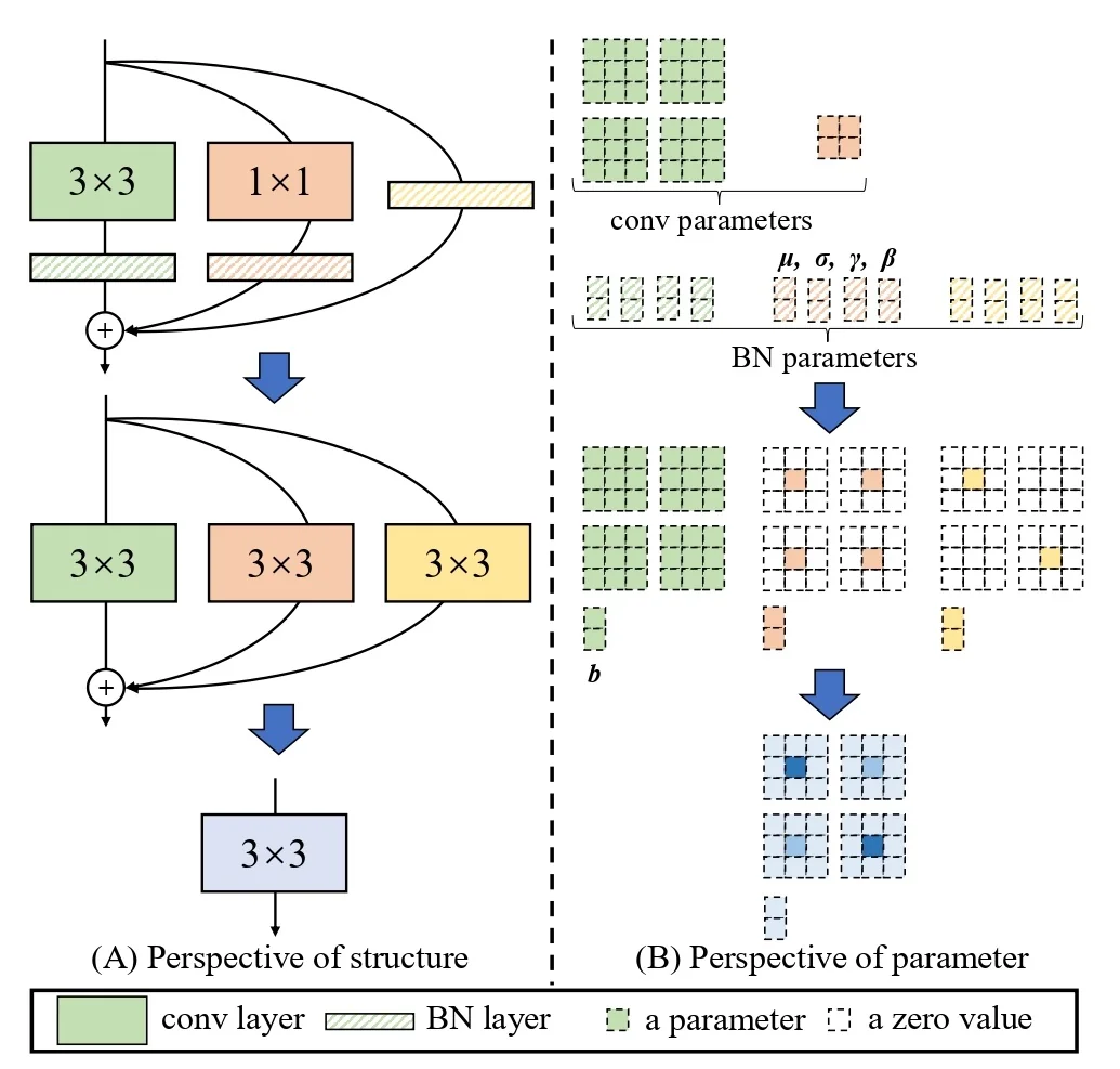
Memory advantages of a plain topology The same conversion that simplifies the operator mix also lowers peak activation memory at inference. In a residual block, the input feature map must remain in memory until the output of the convolutional branch is computed and added back, so the peak activation memory within the block is roughly twice the input size (ignoring parameters). In a plain block, intermediate inputs can be discarded once the next layer finishes. This difference, illustrated in the following figure, motivates RepVGG’s emphasis on a plain inference-time graph not only for speed but also for memory efficiency and specialized hardware design.
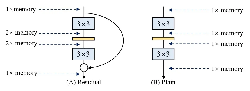
Pseudocode for block re-parameterization The official RepVGG implementation exposes a switch_to_deploy method that replaces each training-time block with its re-parameterized equivalent. The following pseudocode, adapted from the public repository2, illustrates the main steps for a single block.
# Pseudocode for re-parameterizing a single RepVGG block
import torch


def fuse_conv_bn(conv_weight, bn_running_mean, bn_running_var,
                 bn_weight, bn_bias, bn_eps):
    # conv_weight: [C_out, C_in, k, k]
    std = torch.sqrt(bn_running_var + bn_eps)          # [C_out]
    scale = (bn_weight / std).reshape(-1, 1, 1, 1)     # [C_out,1,1,1]
    fused_weight = conv_weight * scale                 # broadcast scale
    fused_bias = bn_bias - bn_running_mean * bn_weight / std
    return fused_weight, fused_bias                    # [C_out,...], [C_out]


def pad_1x1_to_3x3(weight_1x1):
    # weight_1x1: [C_out, C_in, 1, 1]
    k3 = torch.zeros((weight_1x1.size(0),
                      weight_1x1.size(1), 3, 3),
                     dtype=weight_1x1.dtype,
                     device=weight_1x1.device)
    k3[:, :, 1:2, 1:2] = weight_1x1                    # center embedding
    return k3


def get_identity_kernel(num_channels):
    # Identity as 1x1 conv: diagonal kernel
    k = torch.zeros((num_channels, num_channels, 1, 1))
    for c in range(num_channels):
        k[c, c, 0, 0] = 1.0
    return k


def reparameterize_block(conv3, bn3, conv1, bn1, id_bn=None):
    # Fuse 3x3 conv + BN
    w3, b3 = fuse_conv_bn(conv3.weight,
                          bn3.running_mean, bn3.running_var,
                          bn3.weight, bn3.bias, bn3.eps)

    # Fuse 1x1 conv + BN (may be None for some blocks)
    if conv1 is not None:
        w1, b1 = fuse_conv_bn(conv1.weight,
                              bn1.running_mean, bn1.running_var,
                              bn1.weight, bn1.bias, bn1.eps)
        w1 = pad_1x1_to_3x3(w1)
    else:
        w1 = 0.0
        b1 = 0.0

    # Fuse identity + BN if present
    if id_bn is not None:
        kid = get_identity_kernel(num_channels=w3.size(1))
        wid, bid = fuse_conv_bn(kid,
                                id_bn.running_mean, id_bn.running_var,
                                id_bn.weight, id_bn.bias, id_bn.eps)
        wid = pad_1x1_to_3x3(wid)
    else:
        wid = 0.0
        bid = 0.0

    # Sum all kernels and biases to get the equivalent 3x3 conv
    w_equiv = w3 + w1 + wid
    b_equiv = b3 + b1 + bid
    return w_equiv, b_equiv
This procedure is applied once after training to produce a “deploy” version of the model whose body consists solely of conventional \(3\times 3\) convolutions with biases and ReLUs, and can then be exported or further optimized with standard toolchains.
Architecture and implementation details
Macro-architecture and stage design RepVGG adopts a classical VGG-style plain topology whose inference-time body is nothing but a stack of \(3\times 3\) convolutions followed by ReLU activations [129]. There are no residual connections, concatenations, depthwise convolutions, or pooling layers inside the body: spatial downsampling is performed exclusively by stride-2 \(3\times 3\) convolutions. The network is organized into five stages operating at progressively reduced resolutions. The first layer of each stage is a stride-2 \(3\times 3\) convolution that halves the spatial resolution, and all remaining layers in that stage are stride-1 \(3\times 3\) convolutions. For ImageNet classification, the convolutional body is followed by global average pooling and a fully connected classifier.
The depth of each stage is chosen according to three simple guidelines that couple accuracy, latency, and parameter count [129]:
- Stage 1 (high resolution). This stage operates on the largest feature maps (\(112\times 112\) for ImageNet) and therefore dominates convolutional latency. To avoid an expensive early bottleneck, Stage 1 is restricted to a single layer.
- Stage 5 (many channels). The final stage has the largest number of channels and thus the highest parameter cost per layer. To limit overall model size, Stage 5 is also restricted to a single layer.
- Stage 4 (main representational capacity). Following ResNet-101 and related architectures, most of the depth is concentrated in the second-to-last stage at resolution \(14\times 14\), which has been empirically important for recognition performance [215]. RepVGG therefore allocates 14–16 layers to Stage 4.
Model families: RepVGG-A vs. RepVGG-B Within this macro-architecture, the authors define two depth configurations, giving rise to the A-series and B-series model families [129]. Both share the same plain topology, block design, and re-parameterization procedure; they differ only in the number of layers per stage:
- RepVGG-A (lightweight and middleweight). This family uses stage depths \((1, 2, 4, 14, 1)\) and is designed to compete with standard backbones such as ResNet-18/34/50 in terms of accuracy and speed.
- RepVGG-B (high performance). This family is deeper in the middle stages, with stage depths \((1, 4, 6, 16, 1)\). The additional layers in Stages 2–4 increase representational capacity and allow RepVGG-B models to rival stronger baselines such as RegNetX-3.2GF/12GF and EfficientNet-B3.
The resulting stage-wise layout is summarized in the following table.
| Stage | Output size | RepVGG-A | RepVGG-B |
| 1 | \(112\times 112\) | \(1\times \min (64,\,64a)\) | \(1\times \min (64,\,64a)\) |
| 2 | \(56\times 56\) | \(2\times 64a\) | \(4\times 64a\) |
| 3 | \(28\times 28\) | \(4\times 128a\) | \(6\times 128a\) |
| 4 | \(14\times 14\) | \(14\times 256a\) | \(16\times 256a\) |
| 5 | \(7\times 7\) | \(1\times 512b\) | \(1\times 512b\) |
Width scaling and named variants RepVGG instantiates a family of concrete models by uniformly scaling the canonical stage widths \([64, 128, 256, 512]\) with two multipliers \(a\) and \(b\) [129]. Stages 2–4 use channel widths \([64a, 128a, 256a]\), and Stage 5 uses \(512b\) channels. The last multiplier is typically larger, \(b > a\), so that the final stage can produce rich, high-dimensional features for classification and downstream tasks without incurring much extra latency (since Stage 5 contains only a single layer).
The first stage is treated specially. Its width is set to \(\min (64, 64a)\), which has two effects: (i) for small models (\(a < 1\)), Stage 1 narrows proportionally, reducing computation at high resolution; and (ii) for larger models (\(a > 1\)), Stage 1 never exceeds 64 channels, preventing overly wide convolutions on the \(112\times 112\) feature maps, which would otherwise dominate inference time.
The following table lists the main ImageNet-training based models, making explicit which family (A or B) each variant belongs to and how its width multipliers are chosen.
| Name | Family | Layers per stage | \((a, b)\) |
| RepVGG-A0 | A | \(1,\,2,\,4,\,14,\,1\) | \((0.75,\,2.5)\) |
| RepVGG-A1 | A | \(1,\,2,\,4,\,14,\,1\) | \((1.0,\,2.5)\) |
| RepVGG-A2 | A | \(1,\,2,\,4,\,14,\,1\) | \((1.5,\,2.75)\) |
| RepVGG-B0 | B | \(1,\,4,\,6,\,16,\,1\) | \((1.0,\,2.5)\) |
| RepVGG-B1 | B | \(1,\,4,\,6,\,16,\,1\) | \((2.0,\,4.0)\) |
| RepVGG-B2 | B | \(1,\,4,\,6,\,16,\,1\) | \((2.5,\,5.0)\) |
| RepVGG-B3 | B | \(1,\,4,\,6,\,16,\,1\) | \((3.0,\,5.0)\) |
Optional interleaved groupwise convolutions To further trade accuracy for efficiency, some RepVGG variants interleave groupwise \(3\times 3\) convolutions with dense ones [129]. Concretely, for the A- and B-series, the authors set the number of groups \(g \in \{1,2,4\}\) for the \(3\)rd, \(5\)th, \(7\)th, …, \(21\)st layers in RepVGG-A and for these plus the extra \(23\)rd, \(25\)th, and \(27\)th layers in RepVGG-B. The corresponding \(1\times 1\) branches use the same number of groups \(g\), ensuring that the structural re-parameterization remains valid.
Adjacent groupwise convolutions are deliberately avoided. If two grouped layers were stacked without an intervening dense convolution, the output channels would depend only on a small subset of input channels, limiting cross-channel information flow—a phenomenon already observed in ShuffleNet [420]. By interleaving groupwise and dense layers, the network can reduce FLOPs and parameters while still allowing global channel mixing over a few layers.
Models that employ such grouped layers are denoted with suffixes such as g2 and g4 (e.g., RepVGG-B1g4), clearly indicating the group size used in those interleaved layers.
Training details for ImageNet classification On ImageNet-1K, the authors use two training regimes, matched to model capacity [129].
For lightweight and middleweight models (RepVGG-A0/A1/A2, B0/B1 and corresponding g2/g4 variants), they adopt a relatively simple 120-epoch schedule:
- Data augmentation. Random resized cropping and horizontal flipping, following the official PyTorch ResNet example.
- Optimization. Stochastic gradient descent with momentum \(0.9\), weight decay \(10^{-4}\), batch size \(256\), and an initial learning rate of \(0.1\) with cosine annealing over 120 epochs.
- Normalization. Standard BatchNorm in every branch, run in inference mode when performing structural re-parameterization so that the accumulated statistics \((\mu ,\sigma )\) can be fused into the convolution kernels and biases.
For heavyweight models (RegNetX-12GF, EfficientNet-B3, and RepVGG-B2/B3 under a stronger 200-epoch setting), they employ a more advanced “bag of tricks”:
- Data augmentation. AutoAugment [113] combined with random cropping and flipping.
- Regularization. Mixup [791], label smoothing, and longer cosine-annealed learning rate schedules with a 5-epoch warmup.
This separation makes it explicit that the largest RepVGG models (RepVGG-B3 and RepVGG-B3g4) rely on both architectural capacity and strong data augmentation/regularization to push plain ConvNets beyond \(80\%\) top-1 accuracy on ImageNet [129].
Conversion to deploy form and speed measurement After training, every RepVGG block is converted into its deploy form—a single \(3\times 3\) convolution with bias—by fusing BatchNorm parameters into the convolution weights, zero-padding \(1\times 1\) and identity kernels to \(3\times 3\), and summing all branches, as described in the previous subsection. The resulting inference-time network is a pure stack of \(3\times 3\) conv+ReLU layers, which is highly optimized on GPU libraries such as cuDNN and well suited for specialized hardware.
To compare runtime fairly, the authors also fuse conv–BatchNorm sequences in baseline models (ResNet, RegNet, EfficientNet) into single convolutions with bias. Speed is measured on a single NVIDIA 1080Ti GPU with batch size 128, full precision (fp32), single-crop evaluation, and 50 warmup batches before timing, under identical software settings for all models [129].
Experiments and ablation studies
Accuracy–speed trade-off on ImageNet The main experimental message of RepVGG is that a plain, VGG-style ConvNet can simultaneously reach state-of-the-art accuracy and deliver substantially higher actual throughput than many multi-branch or depthwise-heavy architectures on the same hardware. On ImageNet-1K, the largest model RepVGG-B3 exceeds \(80\%\) top-1 accuracy, to the authors’ knowledge the first time a plain ConvNet has crossed this milestone, while retaining a simple inference graph composed only of \(3\times 3\) convolutions and ReLUs [129].
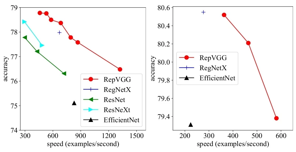
A key observation in these experiments is that theoretical FLOPs are a poor proxy for wall-clock speed. For example, VGG-16 has \(8.4\times \) the FLOPs of EfficientNet-B3 but nevertheless runs \(1.8\times \) faster on the same 1080Ti GPU, implying roughly \(15\times \) higher effective computational density (the product of theoretical FLOPs and measured speed, i.e., TFLOPS) for this dense VGG-style \(3\times 3\) convolutional architecture [129]. RepVGG exploits this regime: by converting its multi-branch training-time blocks into a plain stack of \(3\times 3\) convolutions, it maximizes the use of highly optimized Winograd convolutions while minimizing overhead from fragmented operators, depthwise convolutions, and complex dataflows.
Compared to classic ResNets, RepVGG models achieve both higher top-1 accuracy and higher throughput under matched training settings [129]:
- RepVGG-A0 vs. ResNet-18. RepVGG-A0 achieves \(1.25\) percentage points higher top-1 accuracy on ImageNet (72.41 vs. 71.16) while running about \(33\%\) faster than ResNet-18.
- RepVGG-A1 vs. ResNet-34. RepVGG-A1 achieves \(0.29\) percentage points higher top-1 accuracy (74.46 vs. 74.17) and runs about \(64\%\) faster than ResNet-34.
- RepVGG-A2 vs. ResNet-50. RepVGG-A2 gains \(0.17\) percentage points in top-1 accuracy (76.48 vs. 76.31) and is roughly \(83\%\) faster than ResNet-50.
- RepVGG-B1g4 vs. ResNet-101. The grouped variant RepVGG-B1g4 achieves \(0.37\) percentage points higher top-1 accuracy (77.58 vs. 77.21) while running about \(101\%\) faster (roughly double the throughput) than ResNet-101.
Against the original VGG-16, RepVGG-B2 achieves \(6.57\%\) higher top-1 accuracy while running about \(10\%\) faster and using only roughly \(58\%\) of the parameters [129]. Compared to EfficientNet-B0/B3 and RegNetX-3.2GF/12GF [621, 514], RepVGG variants reach competitive or better accuracy while maintaining substantially higher measured throughput, despite in some cases having larger nominal FLOPs; this gap is precisely what the authors attribute to computational density and the simplicity of the operator set.
Semantic segmentation on Cityscapes To test RepVGG as a generic backbone, the authors plug RepVGG-B1g2 and RepVGG-B2 into a PSPNet-style semantic segmentation model on Cityscapes [808, 129]. Replacing ResNet-50/101 backbones with RepVGG backbones improves mean IoU (mIoU) while also reducing inference time under identical training and decoding settings. For example, the RepVGG-B1g2-fast backbone (with dilation applied only in the last five layers) surpasses a ResNet-101 backbone by \(0.37\) mIoU points and runs \(62\%\) faster on the same 1080Ti GPU [129]. Larger backbones such as RepVGG-B2 and B2-fast further improve mIoU while retaining a favorable speed advantage, indicating that the plain inference topology produced by structural re-parameterization preserves the mid-level features required for dense prediction.
Ablation on branches and structural re-parameterization A central question is whether RepVGG’s gains come merely from its final plain architecture or specifically from training with a multi-branch block that is later re-parameterized. Ablation studies on RepVGG-B0 (trained on ImageNet for 120 epochs) show that the training-time branches are crucial [129]. When both the identity and \(1\times 1\) branches are removed, the model degenerates into a plain stack of \(3\times 3\)-BN-ReLU layers and achieves only \(72.39\%\) top-1 accuracy. Adding back a single branch already helps: using only the \(1\times 1\) branch yields \(73.15\%\), and using only the identity branch yields \(74.79\%\).
The full three-branch RepVGG-B0 block, with both identity and \(1\times 1\) branches, reaches \(75.14\%\) top-1 accuracy. Importantly, because all these variants are converted to the same plain \(3\times 3\) architecture at test time, these differences can only be attributed to the training-time topology and dataflow.
The authors further compare RepVGG-B0 with several re-parameterization baselines [771, 128, 129]. A DiracNet-style model, which re-parameterizes convolution kernels but does not introduce an actual multi-branch structure, attains \(73.97\%\) top-1 accuracy. ACNet’s asymmetric convolution blocks, which over-parameterize each conv at the component level, reach \(73.58\%\), despite using more parameters than RepVGG-B0. A “Residual Reorg” baseline that rearranges the same convolutions and BatchNorm layers into a standard two-branch residual topology (similar to ResNet-18/34) achieves \(74.56\%\), still below RepVGG-B0’s \(75.14\%\). The authors interpret this gap using an implicit-ensemble view: with 15 three-branch blocks in Stage 4, RepVGG behaves like an ensemble of \(2\times 3^{15} \approx 2.8\times 10^7\) sub-models, whereas the Residual Reorg network (with two branches per block) corresponds to only \(2^8 = 256\) sub-models in that stage [129, 665]. This perspective reinforces that the training-time multi-branch structure, not just the final plain architecture, is key to RepVGG’s accuracy.
Effect of BatchNorm placement and extra nonlinearities The structural re-parameterization procedure requires that each branch remains strictly linear up to its BatchNorm and that all BatchNorm layers be applied before branch summation. Empirically, moving BatchNorm to after the addition (a post-addition BN) reduces ImageNet top-1 accuracy from \(75.14\%\) to \(73.52\%\), and removing BatchNorm from the identity branch drops it to \(74.18\%\) [129]. Inserting additional ReLU nonlinearities inside the branches (after BN and before addition) slightly improves accuracy to \(75.69\%\), but breaks the exact algebraic equivalence needed to collapse the block into a single convolution at inference. Thus, the block design is tightly constrained by the deployment goal: branches must be linear up to BN, and BN must sit immediately after each convolution and before summation.
Groupwise convolution trade-offs Finally, RepVGG-B1g2/B1g4 and B2g2/B2g4 introduce interleaved groupwise \(3\times 3\) convolutions as an additional accuracy–efficiency knob. Every third \(3\times 3\) layer in the main branch (and its corresponding \(1\times 1\) branch) is converted into a groupwise convolution, while adjacent groupwise layers are avoided to preserve inter-channel information exchange [420, 129]. These grouped variants typically sacrifice only a small amount of accuracy (e.g., RepVGG-B1g4 at \(77.58\%\) vs. B1 at \(78.37\%\)) while yielding substantial speedups (868 vs. 685 images/second on a 1080Ti, respectively). In particular, RepVGG-B1g4 is both \(0.37\%\) more accurate and roughly twice as fast as ResNet-101, and RepVGG-B1g2 matches the accuracy of ResNet-152 while being \(2.66\times \) faster [129]. Overall, the experiments show that RepVGG provides a flexible, structurally simple template whose operating point along the accuracy–speed curve can be adjusted via depth, width, and grouping, without ever compromising the plain inference-time topology.
Limitations and future directions
Inference efficiency is tailored to \(3\times 3\) convolutions RepVGG’s strength is its uniform use of \(3\times 3\) convolutions at inference, which aligns well with cuDNN/MKL optimizations and with specialized hardware that can implement large numbers of identical \(3\times 3\)-ReLU units [129].
This design is ideal for throughput-oriented GPUs and accelerators but may not always be optimal on mobile NPUs or very low-power microcontrollers where depthwise separable convolutions or highly compressed operators (e.g., as in MobileNetV4 or GhostNet-style blocks) can be more attractive. In extremely tight memory or power budgets, RepVGG’s relatively large number of parameters compared to some mobile-optimized models can also be limiting.
Constraints on training-time topology Because structural re-parameterization relies on exact algebraic equivalence, the training-time block topology is tightly constrained. Branches must be purely linear up to BatchNorm and must share compatible strides and padding; nonlinearities, attention modules (such as SE blocks [244]), or more exotic operators inside branches would break the exact conversion to a single \(3\times 3\) convolution. This limits the ability to combine RepVGG-style re-parameterization with some of the more advanced components used in ConvNeXt/ConvNeXtV2 [400, 721], NFNets [54], or MobileNetV4.
Interaction with design spaces and NAS RepVGG instantiates its architecture using simple heuristic design rules rather than exhaustive architecture search or design spaces such as RegNet [514] or MobileNetV4’s unified inner-block (UIB) [507]. In that sense, the paper demonstrates the viability of a plain, re-parameterized architecture rather than claiming optimality in the broader architecture space. Future work can combine structural re-parameterization with design spaces or neural architecture search, exploring plain inference-time networks that are optimized jointly over depth, width, grouping, and training-time branch topology.
Beyond small kernels and single-image tasks The structural re-parameterization used in RepVGG is conceptually general: any linear multi-branch structure with compatible spatial supports and BatchNorm layers can be merged into a single convolution. Subsequent work has explored larger kernels, asymmetric kernels, and multi-scale kernels using similar ideas (e.g., ACNet’s asymmetric convolutions [128]), and there is room to extend these techniques to very large receptive fields, 3D convolutions, or multi-frame video backbones. In Chapter Enrichment 11.12 and later sections, structural re-parameterization will reappear in the context of Rep-style large-kernel networks and hybrid ConvNet–Transformer designs, illustrating how RepVGG’s core idea can be a building block in more complex systems.
Role within the broader ConvNet design landscape In the high-level summary at the end of this chapter, RepVGG exemplifies the design philosophy of training–inference decoupling:
- Optimization uses a rich multi-branch topology. During training, RepVGG leverages ResNet-style identities and additional \(1\times 1\) branches to behave like an implicit ensemble of many shallower models, improving gradient flow and convergence.
- Deployment uses a plain \(3\times 3\) stack. For inference, structural re-parameterization collapses the multi-branch blocks into a VGG-style stack of \(3\times 3\)-ReLU layers that is well suited to hardware, fast in practice, and easy to integrate into existing codebases.
Together with ConvNeXt/ConvNeXtV2 for modernization and scaling, MobileNetV4 for hardware-aware unification, and GhostNet-style cheap feature generation, RepVGG provides a concrete and practically relevant example of how decoupling training and inference architectures can reconcile optimization needs with deployment constraints in modern ConvNets.
11.13 Summary of Efficient Network Architectures
This chapter has explored a broad spectrum of CNN design innovations, from early residual and attention mechanisms to modern, Transformer-era ConvNets. Across these developments, the central goal has remained the same: improve both theoretical efficiency (FLOPs, parameter counts, scaling laws) and practical efficiency (latency, memory bandwidth, hardware utilization). We now summarize the main architectural milestones and the key lessons that emerge.
Grouped convolutions and ResNeXt
ResNeXt extended the ResNet bottleneck design by introducing grouped convolutions, allowing multiple parallel transformations at a fixed FLOP budget. The notion of cardinality (number of groups) became a new degree of freedom, often yielding better accuracy than deeper or wider ResNets at similar cost. However, ResNeXt still followed conventional design heuristics (e.g., doubling channels when halving spatial resolution) and did not directly optimize memory usage or hardware-friendliness.
Squeeze-and-Excitation (SE) blocks
SE blocks introduced channel-wise attention, yielding significant accuracy gains for minimal additional computation by learning to recalibrate channel responses. At the same time, SE operations (global pooling, a small MLP, and channel-wise scaling) did not always map cleanly to certain edge devices. Later architectures (for example, EfficientNet-Lite) removed SE blocks to improve real-world deployment speed on mobile hardware.
MobileNet and ShuffleNet: depthwise separable convolutions and channel mixing
MobileNetV1 popularized depthwise separable convolutions, drastically reducing FLOPs by decomposing a standard convolution into a depthwise convolution followed by a pointwise \(1\times 1\) convolution. However, these depthwise operators often underutilized GPU hardware and, on their own, struggled to mix channel information effectively. ShuffleNet refined channel mixing via channel shuffling combined with group convolutions, achieving better accuracy at the same theoretical complexity, though in practice it was not always faster due to non-trivial memory access patterns.
MobileNetV2: inverted residual blocks
MobileNetV2 introduced inverted residuals with linear bottlenecks, applying nonlinearity only in the high-dimensional expanded space and using linear projections for the narrow bottlenecks. This prevented information collapse and made each block more expressive despite higher per-layer cost. As a result, MobileNetV2 networks could be shallower yet more powerful overall, becoming a standard template for mobile backbones.
NAS and MobileNetV3, ShuffleNetV2 insights
Neural Architecture Search (NAS) was used to construct MobileNetV3, combining inverted bottlenecks, SE blocks, and specialized activations (e.g., h-swish) for a strong accuracy–FLOP trade-off. In parallel, ShuffleNetV2 proposed hardware-friendly design guidelines (uniform channel widths, minimal group convolutions, avoiding fragmentation, etc.) derived from empirical latency studies. In practice, MobileNetV3 achieved superior accuracy and became widely adopted, but it remained imperfectly aligned with all hardware. It was also not especially scalable: deeper MobileNetV3 variants sometimes exhibited sub-optimal or even diminishing returns as depth increased.
GhostNet: exploiting feature redundancy
GhostNet focuses on feature redundancy. In many standard convolutional layers, a significant fraction of output channels are highly correlated and can be viewed as “ghosts” of a smaller intrinsic set (for example, scaled or filtered copies).
GhostNet introduces the Ghost module:
- A standard convolution first produces a relatively small number of intrinsic feature maps.
- Lightweight depthwise convolutions are then applied to these maps to generate additional ghost feature maps via simple linear transformations.
By concatenating intrinsic and ghost features, Ghost modules approximate the representational capacity of a wider layer at a fraction of the cost. GhostNet and its successors remain popular in extremely tight FLOP and power budgets, and they are natural companions to MobileNet-style designs when targeting microcontrollers and other severely resource-constrained devices.
EfficientNet: compound scaling
EfficientNet introduced compound scaling, a method for jointly scaling depth, width, and resolution in a principled way. Instead of arbitrarily increasing a single dimension, EfficientNet scaled all three simultaneously using learned scaling coefficients. Starting from a NAS-discovered backbone (EfficientNet-B0), this approach yielded state-of-the-art accuracy per FLOP, outperforming many manually designed architectures.
Despite its theoretical efficiency, EfficientNet’s compound scaling was not always optimal for real-world speed. The heavy use of depthwise convolutions and SE blocks incurred non-trivial memory access costs, making inference slower than expected on GPUs and some mobile devices.
To address these issues, optimized variants were introduced.
EfficientNet-Lite and EfficientNetV2
EfficientNet-Lite was designed specifically for mobile deployment by removing SE blocks and replacing h-swish activations with ReLU6, which is more efficient on typical edge hardware. These modifications improved inference latency while retaining most of EfficientNet’s accuracy advantages.
EfficientNetV2 targeted improved training and inference efficiency on GPUs and TPUs. It introduced:
- Fused inverted bottlenecks (Fused-IB) in early stages, which collapse the \(1\times 1\) expansion and depthwise convolution into a single regular \(k\times k\) convolution, reducing memory traffic and kernel launch overhead.
- Progressive learning, where training begins with small input resolutions and gradually increases them, reducing memory consumption, improving convergence, and shortening training time while preserving final accuracy.
Together, these refinements made EfficientNetV2 significantly faster to train and deploy on accelerators, while EfficientNet-Lite improved real-world efficiency on mobile devices.
NFNets: BN-free training
Normalization-Free Networks (NFNets) demonstrated that deep residual networks can be trained without batch normalization by normalizing weights rather than activations. This removes BN’s dependence on large batch sizes and simplifies certain deployment scenarios. However, NFNets require careful variance control, including techniques such as weight standardization and adaptive gradient clipping. In many settings, NFNets trade additional FLOPs and more involved training recipes for the ability to avoid batch normalization entirely.
Revisiting ResNets: scaling and training recipes
ResNet-RS and other carefully tuned ResNet variants showed that, with up-to-date training techniques (longer schedules, stronger regularization and data augmentation, better learning rate schedules), classical ResNets can rival or surpass “state-of-the-art” efficient architectures in both speed and accuracy. These results emphasize that training recipes and data often matter as much as architectural novelty.
RegNets: optimizing the design space
RegNets offered an alternative to computationally expensive NAS. They defined simple, parameterized network families (for example, via channel growth rates and depth rules) and optimized within this low-dimensional design space. This reduced architecture search to a handful of continuous parameters, achieving strong performance at much lower search cost and providing an interpretable bridge between manual design and full NAS.
ConvNeXt and ConvNeXt V2: modernizing the standard
As Vision Transformers began to dominate benchmarks, the ConvNeXt family revisited the standard ResNet and asked whether a pure ConvNet could match Transformer-like performance by adopting modern design practices. ConvNeXt:
- Replaces the early ResNet stem with a patchify convolution (for example, \(4\times 4\) with stride 4) analogous to ViT patch embeddings.
- Uses large-kernel depthwise convolutions and inverted bottlenecks with LayerNorm and GELU to mimic Transformer MLP blocks.
- Simplifies the stage structure to resemble Swin/ViT-style hierarchies.
ConvNeXt V2 extends this modernization to the pretraining regime. By coupling ConvNeXt backbones with a Fully Convolutional Masked Autoencoder (FCMAE) and introducing Global Response Normalization (GRN) to stabilize masked image modeling, ConvNeXt V2 demonstrates that ConvNets can also scale effectively under self-supervised pretraining, not just under supervised ImageNet training. In later chapters, ConvNeXt and ConvNeXt V2 will serve as canonical examples of “modern” ConvNets that compete directly with ViT-style models.
MobileNetV4: universal, roofline-aware mobile models
Earlier MobileNets (V1–V3), ShuffleNet variants, GhostNet, and even a subsequent wave of lightweight Vision Transformers (e.g., MobileViT, LeViT, EdgeViT, FastViT, EfficientViT) were typically tuned to specific devices or operator sets. On some mobile GPUs and NPUs, these mobile Transformers could outperform same-latency ConvNets by exploiting efficient attention kernels, while on DSPs and pure CPUs carefully tuned ConvNets often remained superior due to different memory access patterns and scalar throughput. This divergence across accelerators created a fragmentation problem: no single family of backbones provided consistently strong Pareto trade-offs across CPUs, DSPs, GPUs, and custom accelerators.
MobileNetV4 addresses this explicitly by optimizing with respect to the Roofline model, which characterizes performance in terms of both arithmetic throughput and memory bandwidth rather than FLOPs alone. The goal is to design a single ConvNet family that remains close to Pareto-optimal under a broad range of compute–memory trade-offs, without running NAS separately for each hardware target.
The core abstraction is the Universal Inverted Bottleneck (UIB), a single super-block template that unifies four important micro-architectures within one searchable design:
- The classic MobileNetV2-style inverted bottleneck (IB).
- A ConvNeXt-style block with depthwise convolution before expansion.
- A feedforward-network (FFN)-like variant.
- A novel ExtraDW variant with additional depthwise convolutions.
All of these share a common interface (same input/output layout and stride pattern), allowing NAS to select among them without changing the surrounding topology.
Instead of benchmarking every candidate on physical hardware, MobileNetV4 uses an analytic roofline latency predictor as the NAS reward. For a given model, it computes a ModelTime score by summing, over layers, the Roofline cost \[ \max \left (\frac {\mbox{MACs}_\ell }{\mbox{PeakMACs}}, \frac {\mbox{Bytes}_\ell }{\mbox{PeakMemBW}}\right ), \] where \(\mbox{PeakMACs}\) and \(\mbox{PeakMemBW}\) encode the arithmetic and memory-bandwidth capabilities of a hypothetical device. By sweeping a single scalar ridge point \[ \mbox{RP} = \frac {\mbox{PeakMACs}}{\mbox{PeakMemBW}} \] over a range of values (for example, from near zero to several hundred MACs/byte), the same architecture can be evaluated under many different compute–memory trade-offs. The search therefore discovers models that lie close to the Pareto frontier simultaneously for CPUs, DSPs, GPUs, and accelerators, without ever measuring real hardware during search. For hybrid ConvNet–Transformer models, MobileNetV4 further introduces Mobile Multi-Query Attention (Mobile MQA), a mobile-optimized variant of multi-query attention that accelerates attention on accelerators, reduces memory usage, with only negligible accuracy loss.
RepVGG: structural re-parameterization for deployment
A persistent tension in network design is that complex, multi-branch architectures are easier to optimize, but simple, sequential architectures are more efficient at inference. RepVGG resolves this via structural re-parameterization:
- During training, each block contains a \(3\times 3\) convolution branch, a \(1\times 1\) convolution branch, and (when channel counts match) an identity branch, which together improve gradient flow and representational capacity.
- At inference, the linearity of convolutions allows these branches to be analytically fused into a single equivalent \(3\times 3\) kernel and bias per block.
The deployed network becomes a plain, VGG-style stack of \(3\times 3\) convolutions that maps extremely well to GPU kernels and low-level libraries. RepVGG thus decouples training-time architecture (rich, multi-branch) from inference-time architecture (simple, highly optimized), providing a useful template for other re-parameterizable designs.
Key takeaways
- FLOPs are not everything. Real-world performance depends critically on kernel fusion, memory access patterns, and parallelism, and depthwise-heavy designs or complex attention mechanisms may have excellent FLOP metrics yet underperform on actual hardware; MobileNetV4 explicitly optimizes for this by balancing compute and memory under a Roofline objective rather than minimizing FLOPs alone.
- Hardware alignment is a first-class design goal. Architectures such as EfficientNetV2 and MobileNetV4 show that explicitly modeling memory bandwidth (via fused inverted bottlenecks or analytic Roofline objectives) is essential for achieving practical speedups on GPUs, TPUs, and mobile SoCs.
- Search spaces matter more than single architectures. NAS-based families (MobileNetV3), structured design spaces (RegNets), and macro-block templates (UIBs in MobileNetV4) emphasize that a well-chosen family of models plus a good search or tuning strategy is often more valuable than a single hand-crafted network.
- Training recipes and pretraining regimes are as important as blocks. ResNet-RS, ConvNeXt/ConvNeXt V2, and NFNets demonstrate that optimization strategies (data augmentation, normalization choices, self-supervised pretraining) can close much of the gap between older and newer architectures.
- Deployment context drives architectural choice. For server-side workloads, ConvNeXt-style backbones provide strong accuracy and compatibility with Transformer-era training; for mobile and embedded devices, MobileNetV4, GhostNet, and related families prioritize operator efficiency and memory; for GPU-bound low-latency inference, RepVGG-style re-parameterized networks offer simple, highly optimized compute graphs.
The current frontier (2024–2025) is therefore characterized by roofline-aware universal ConvNets (MobileNetV4), fully convolutional modern ResNets (ConvNeXt V2), and structurally re-parameterized plain networks (RepVGG-style), with lightweight mobile Vision Transformers remaining competitive on certain accelerators. Rather than a single “best” network, modern CNN design offers a toolkit of architectural motifs—residual connections, depthwise separability, channel attention, compound scaling, structural re-parameterization, and roofline-aware macro-blocks—that can be combined and adapted to match the constraints of a given application and hardware platform. In subsequent chapters, many of the detection, segmentation, and 3D vision systems we study will build directly on these backbones, making it crucial to understand both their strengths and their trade-offs.