Lecture 7: Convolutional Networks
7.1 Introduction: The Limitations of Fully-Connected Networks
So far, we have explored linear classifiers and fully-connected neural networks. While fully-connected networks are significantly more expressive than simple linear classifiers, they still suffer from a major limitation: they do not preserve the 2D spatial structure of image data.
These models require us to flatten an image into a one-dimensional vector, losing all spatial relationships between pixels. This is problematic for tasks like image classification, where local patterns such as edges and textures are crucial for understanding an image.
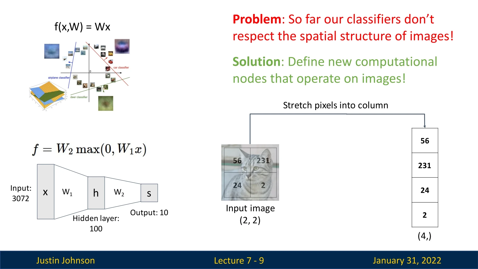
To address this issue, Convolutional Neural Networks (CNNs) introduce new types of layers designed to process images while maintaining their spatial properties.
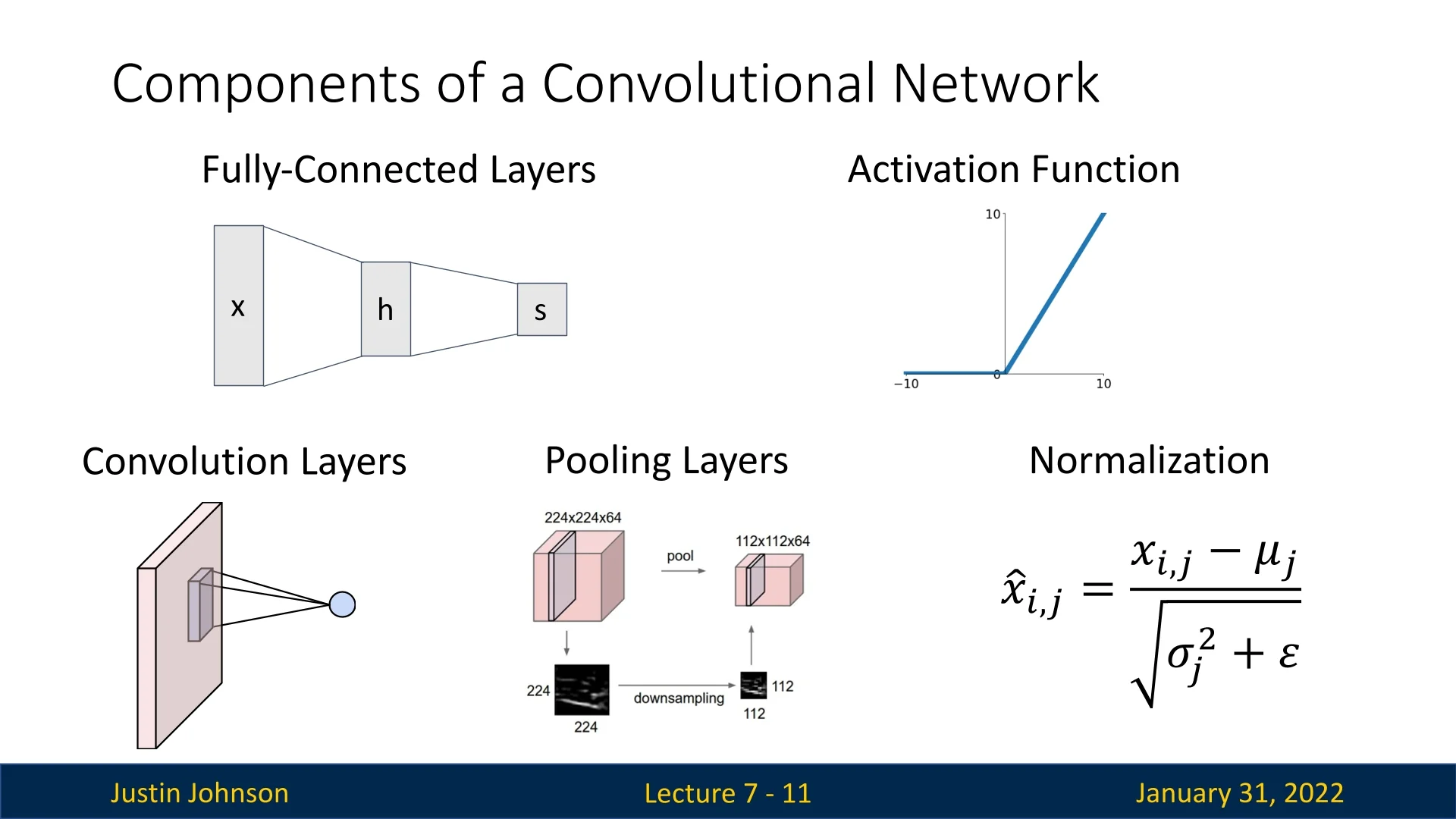
7.2 Components of Convolutional Neural Networks
CNNs extend fully-connected networks by introducing the following specialized layers:
- 1.
- Convolutional Layers: Preserve spatial structure and detect patterns using filters (kernels) that slide across the image.
- 2.
- Pooling Layers: Reduce spatial dimensions while retaining essential features.
- 3.
- Normalization Layers (e.g., Batch Normalization): Stabilize training and improve performance.
These layers allow CNNs to effectively capture hierarchical features from images, making them highly effective for computer vision tasks.
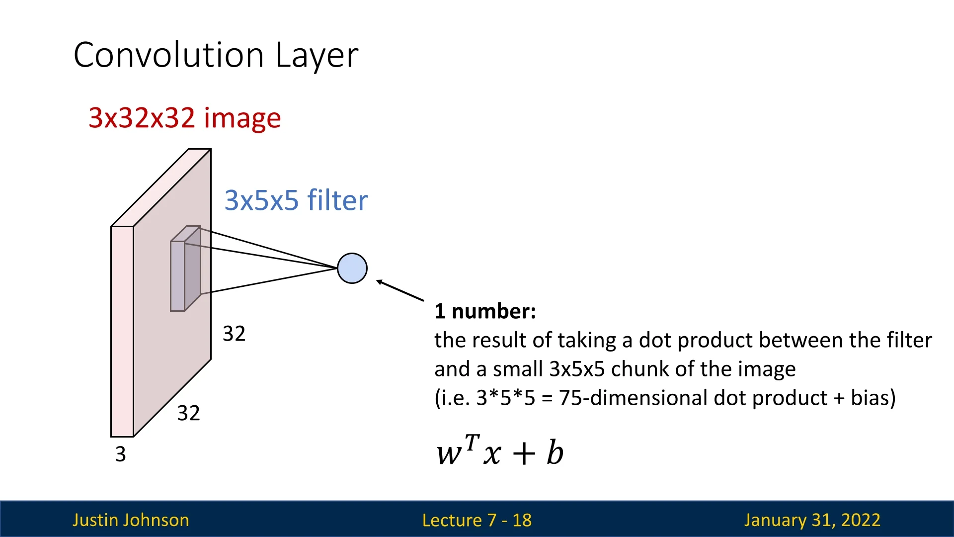
7.3 Convolutional Layers: Preserving Spatial Structure
A convolutional layer is designed to process images while maintaining their 2D structure. Instead of flattening the image into a single vector, convolutional layers operate on small local patches of the input, capturing spatially localized patterns such as edges, corners, and textures.
7.3.1 Input and Output Dimensions
A convolutional layer processes an input tensor while preserving its spatial structure. Unlike fully connected layers, which flatten the input into a vector, convolutional layers operate directly on structured data, maintaining spatial relationships between pixels.
The input to a convolutional layer typically has the shape: \[ C_{\mbox{in}} \times H \times W \] where:
- \(C_{\mbox{in}}\) is the number of input channels (e.g., 3 for an RGB image, where each channel corresponds to red, green, or blue intensity),
- \(H\) and \(W\) represent the height and width of the input image or feature map (a 2D representation of extracted features).
The layer applies a set of filters (also called kernels), where each filter has the shape: \[ C_{\mbox{in}} \times K_h \times K_w. \] Here:
- \(K_h\) and \(K_w\) define the spatial size (height and width) of the filter,
- Each filter always spans all \(C_{\mbox{in}}\) input channels, meaning it processes all color or feature layers together.
Common Filter Sizes Typically, \(K_h\) and \(K_w\) are small, such as 3, 5, or 7, to detect fine-grained patterns while maintaining computational efficiency. Most convolutional layers use square filters (\(K_h = K_w\)), though some architectures employ non-square kernels for specialized feature extraction. For example, Google’s Inception architecture, which we will explore later, uses asymmetric convolutions such as \(1 \times 3\) and \(3 \times 1\) to improve computational efficiency while maintaining expressive power.
Why Are Kernel Sizes Typically Odd? While convolution kernels can have even or odd dimensions, odd-sized kernels (\(3 \times 3\), \(5 \times 5\)) are commonly used due to their advantages in preserving spatial structure and ensuring consistent feature extraction.
- Preserving Spatial Alignment: Odd-sized kernels naturally align with a central pixel, ensuring that the output remains centered relative to the input. This prevents unintended shifts in feature maps, which could cause misalignment across layers and disrupt learning.
- Consistent Neighboring Context: When stacking multiple convolutional layers, each output pixel is influenced symmetrically by its surrounding pixels. This balanced context stabilizes feature learning and helps capture hierarchical patterns effectively.
Even-sized kernels (e.g., \(2 \times 2\), \(4 \times 4\)) do not have a single center pixel, requiring additional adjustments when aligning the filter to the input, and are hence not common.
7.3.2 Filter Application and Output Calculation
Each filter slides (convolves) over the spatial dimensions of the image, computing a dot product between its weights and the corresponding patch of the input at each position. The sum of these dot products, plus a bias term, produces the activation for that position.
Mathematically, for a given position \((i, j)\), the convolution operation computes: \[ y_{i,j} = \sum _{c=1}^{C_{\mbox{in}}} \sum _{m=1}^{K_h} \sum _{n=1}^{K_w} W_{c,m,n} \cdot X_{c, i+m, j+n} + b \] where:
- \( W_{c,m,n} \) represents the filter weights.
- \( X_{c, i+m, j+n} \) represents the corresponding region of the input image.
- \( b \) is the bias term.
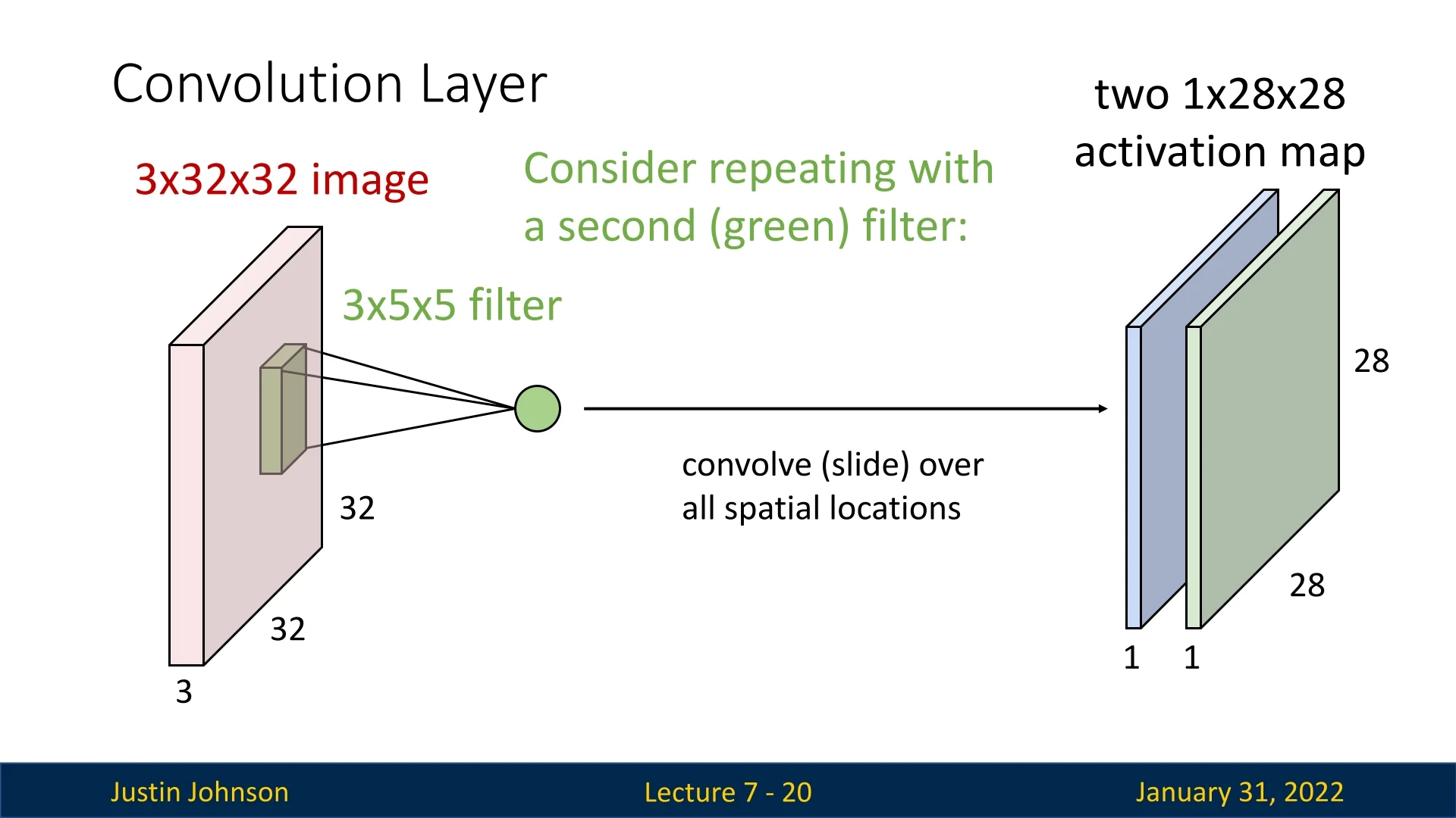
Each filter produces a single activation map, and stacking multiple filters results in a 3D output tensor.
Enrichment 7.3.3: Understanding Convolution Through the Sobel Operator
To build intuition for convolutional operations, we start with a simple example: applying a \(3 \times 3\) 2D filter to a single-channel (\(C_{\mbox{in}} = 1\)) grayscale image. Later we’ll dive into more practical examples, to better understand how convolutional layers work. More specifically, we’ll cover how such layers work with several multi-channel filters applied to the input image, integrated along with their corresponding biases, along with other mechanisms like strides/padding (larger than 1), that are often seen in conv-nets.
Enrichment 7.3.3.1: Using the Sobel Kernel for Edge Detection
A widely used filter for detecting edges in images is the Sobel operator, which approximates the image gradient along the horizontal and vertical directions. This filter is based on the concept of central differences, a discrete method for estimating gradients in a sampled function—such as an image.
Approximating Image Gradients with the Sobel Operator To estimate the gradient at each pixel, we can use a basic finite difference approach. The simplest method is the forward difference, which approximates the derivative at a given pixel by computing the difference between its right neighbor and itself. However, this method introduces a shift in the computed gradient locations. A more accurate approach is the central difference, which averages the difference between the left and right neighbors:
\[ \frac {\partial I}{\partial x} \approx \frac {I(x+1, y) - I(x-1, y)}{2}. \]
Similarly, for the vertical gradient:
\[ \frac {\partial I}{\partial y} \approx \frac {I(x, y+1) - I(x, y-1)}{2}. \]
These central difference approximations form the basis of the gradient operators used in edge detection.
Basic Difference Operators A simple discrete implementation of the central difference method would use the following filters:
\[ \mbox{Diff}_x = \begin {bmatrix} -1 & 0 & 1 \\ -1 & 0 & 1 \\ -1 & 0 & 1 \end {bmatrix}, \quad \mbox{Diff}_y = \begin {bmatrix} -1 & -1 & -1 \\ 0 & 0 & 0 \\ 1 & 1 & 1 \end {bmatrix}. \]
These filters compute intensity differences between neighboring pixels along the horizontal and vertical axes, highlighting abrupt changes. However, they treat all pixels equally, making them highly sensitive to noise. A small random fluctuation in intensity could result in large, unstable gradient estimates.
The Sobel Filters: Adding Robustness The Sobel filters improve upon these simple difference operators by incorporating a Gaussian-like weighting to give more importance to the central pixels:
\[ \mbox{Sobel}_x = \begin {bmatrix} 1 \\ 2 \\ 1 \end {bmatrix} \begin {bmatrix} 1 & 0 & -1 \end {bmatrix} = \begin {bmatrix} 1 & 0 & -1 \\ 2 & 0 & -2 \\ 1 & 0 & -1 \end {bmatrix} \]
\[ \mbox{Sobel}_y = \begin {bmatrix} 1 \\ 0 \\ -1 \end {bmatrix} \begin {bmatrix} 1 & 2 & 1 \end {bmatrix} = \begin {bmatrix} 1 & 2 & 1 \\ 0 & 0 & 0 \\ -1 & -2 & -1 \end {bmatrix} \]
Enrichment 7.3.3.2: Why Does the Sobel Filter Use These Weights?
- Improving Gradient Accuracy: The \([-1, 0, 1]\) pattern in \(\mbox{Sobel}_x\) is a discrete approximation of the central difference derivative, meaning it captures intensity changes along the horizontal axis, responding to vertical edges. Similarly, \(\mbox{Sobel}_y\) captures intensity changes along the vertical axis, detecting horizontal edges.
- Smoothing High-Frequency Noise: The \([1, 2, 1]\) weighting acts as a mild low-pass filter, averaging nearby pixels to reduce noise sensitivity while maintaining edge sharpness.
- Preserving Image Structure: The use of a larger weight at the center (\(2\)) ensures that local gradient computations are less affected by isolated pixel noise and instead capture broader edge structures.
Enrichment 7.3.3.3: Computing the Gradient Magnitude
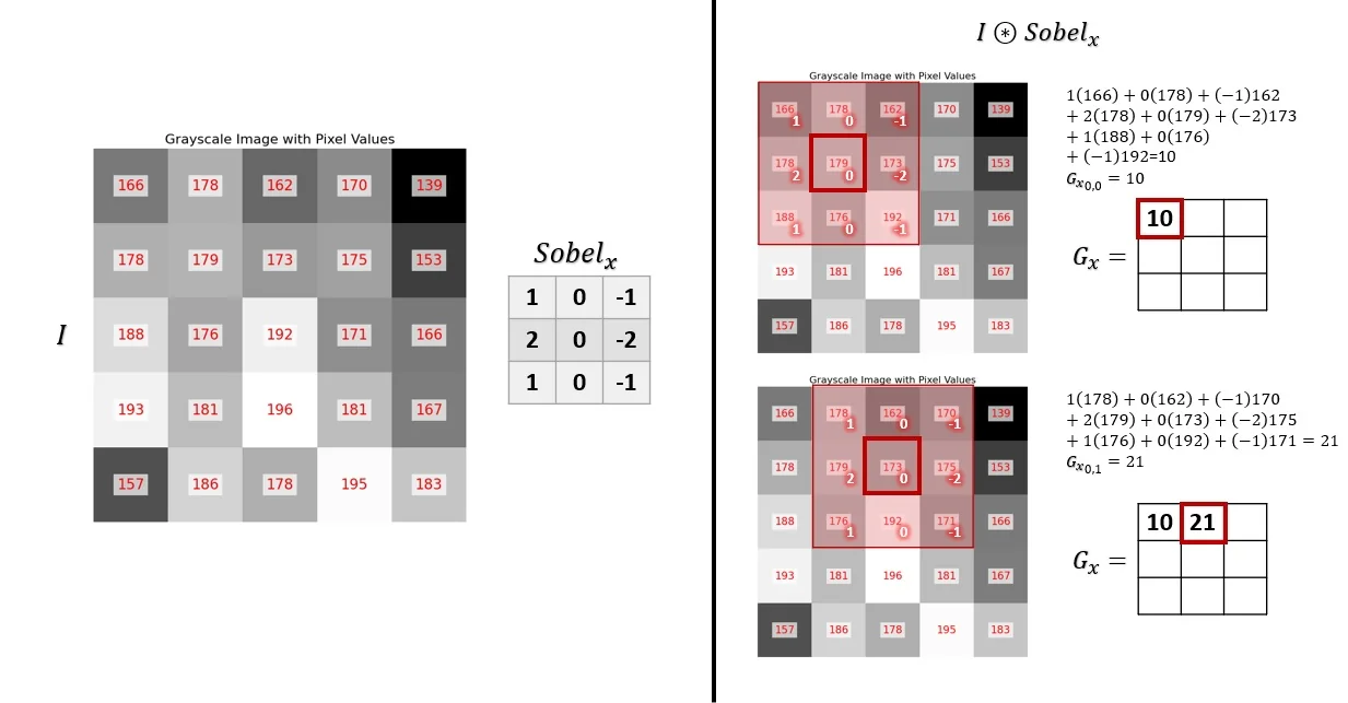
At each spatial location in the image, the kernel is positioned over a \(3 \times 3\) region of pixel intensities. The convolution operation computes the dot product between the kernel and the underlying pixel values, yielding a new intensity that reflects the local gradient in the selected direction.
Applying \(\mbox{Sobel}_x\) results in an edge map \(G_x=I * \mbox{Sobel}_x\), where larger absolute values indicate strong vertical edges (intensity changes along the horizontal direction). Similarly, applying \(\mbox{Sobel}_y\) results in an edge map \(G_y=I * \mbox{Sobel}_y\), where larger absolute values indicate strong horizontal edges (intensity changes along the vertical direction).
To combine both directions, we compute the gradient magnitude:
\[ G = \sqrt {G_x ^2 + G_y ^2}. \]
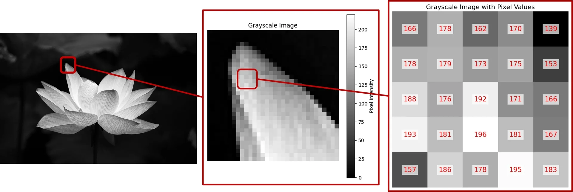
To better understand the effect of convolution with the Sobel filter, consider an example grayscale image where distinct edges are present. As the kernel slides over the image:
- Areas with constant intensity produce near-zero outputs (low gradient).
- Regions with sudden changes in intensity (edges) produce large values, indicating strong gradients.
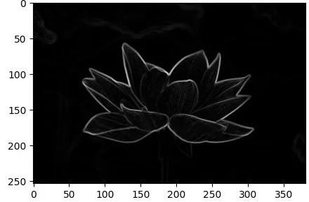
We will proceed to visualize this process, taking the cropped zoom-in part of the original image as seen in Figure 7.5. We’ll first examine the computation using a single filter channel \(\mbox{Sobel}_x\), convolved with the cropped patch.
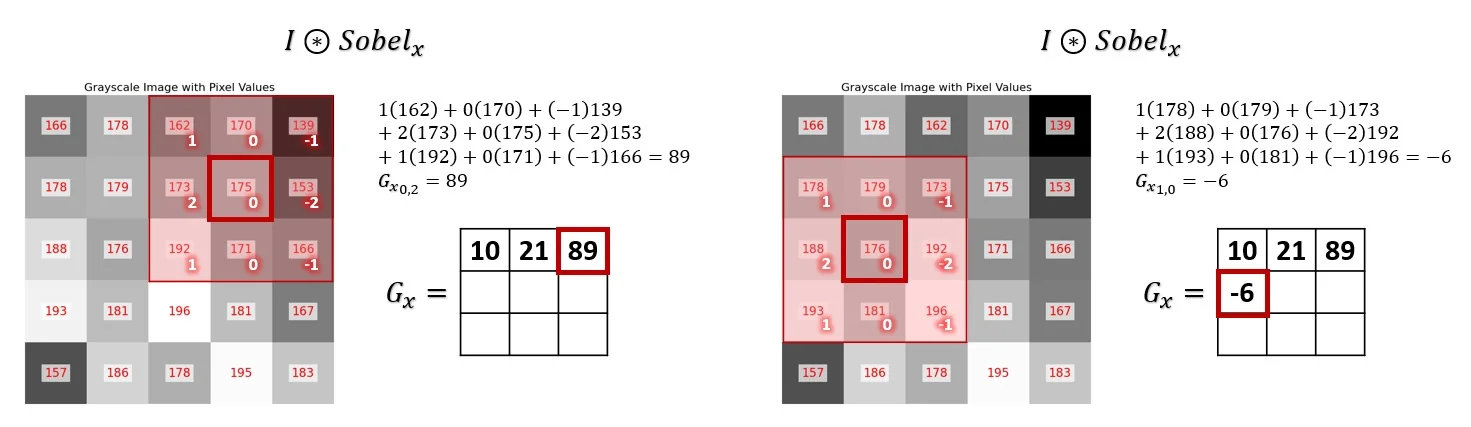
At the end of this process, we obtain an output in the form of a 2D edge map, \(G_x\), where larger absolute values correspond to pixels that are likely part of a vertical edge (corresponding to large gradients along the horizontal axis of the image). The same process can be done with the other single-filter channel \(\mbox{Sobel}_y\), resulting in \(G_y\), where larger absolute values correspond to horizontal edges.
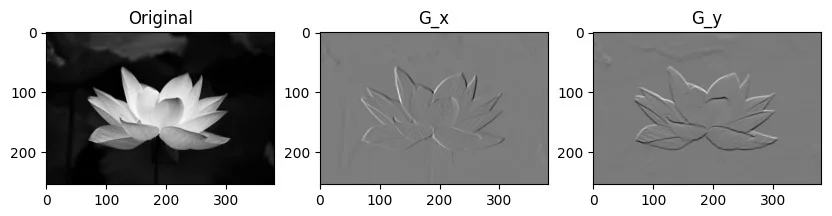
We can apply this process to the entire image, obtaining the full edge maps \(G_x\) and \(G_y\). By combining them, we get a single edge image:
\[ G = \sqrt {G_x ^2 + G_y ^2}. \]
Convolutional layers in neural networks use this operation to extract meaningful features, such as edges and textures, which serve as the foundation for deeper representations. While neural networks learn their own filters during training, edge-detecting filters like Sobel demonstrate how convolution naturally captures important structural information.
Hands-On Exploration To build deeper intuition around convolutions, it can be enlightening to interactively apply various kernels to images. One accessible resource is Setosa’s Image Kernels Demo, where you can hover over a grayscale image and experiment with different filters like the Sobel filter on the fly. Tinkering in this way helps illustrate how individual convolutional kernels isolate specific visual features and produce characteristic activation patterns.
Enrichment 7.4: Convolutional Layers with Multi-Channel Filters
Previously, in 7.3.2, we explored how convolution operates using a single \(3 \times 3\) 2D filter. Now, we extend this concept to multi-channel inputs, such as RGB images, which contain multiple color channels. Convolutional layers typically consist of multiple multi-dimensional filters, each spanning all input channels. Additionally, each filter has an associated bias term in the bias vector \(\mathbf {b}\), which is added to the convolution result to introduce additional flexibility.
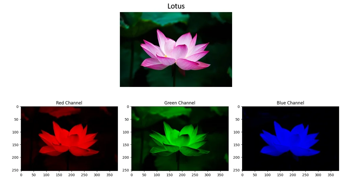
To illustrate this extension, we consider an RGB image of a Lotus flower. Unlike grayscale images, which contain a single intensity channel, RGB images have three channels—red, green, and blue—each containing spatial information about the corresponding color component.
Enrichment 7.4.1: Extending Convolution to Multi-Channel Inputs
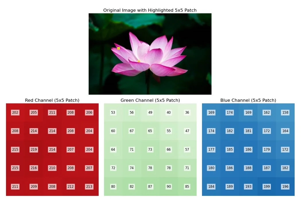
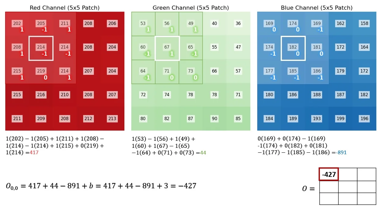
To demonstrate multi-channel convolution, consider a randomly selected \(5 \times 5\) patch from the image along with a single randomly initialized \(3\)-channel filter.
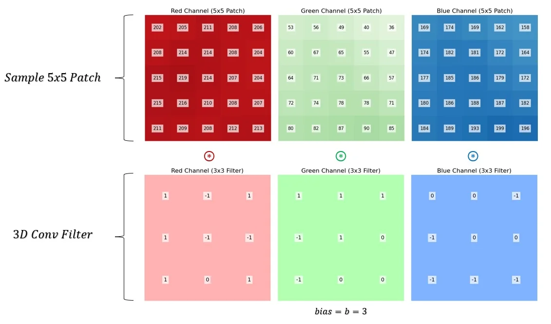
Multi-Channel Convolution Process When performing convolution on multi-channel images, each filter is applied separately to each channel, and the results are summed to produce a single output value for each spatial position. This is equivalent to computing multiple 2D convolutions (one per input channel) and then aggregating the results.
- Each channel of the filter is convolved with its corresponding channel in the input patch.
- The outputs from all channels are summed together at each spatial location.
- A bias term associated with the filter is added to the summed result.
Sliding the Filter Across the Image
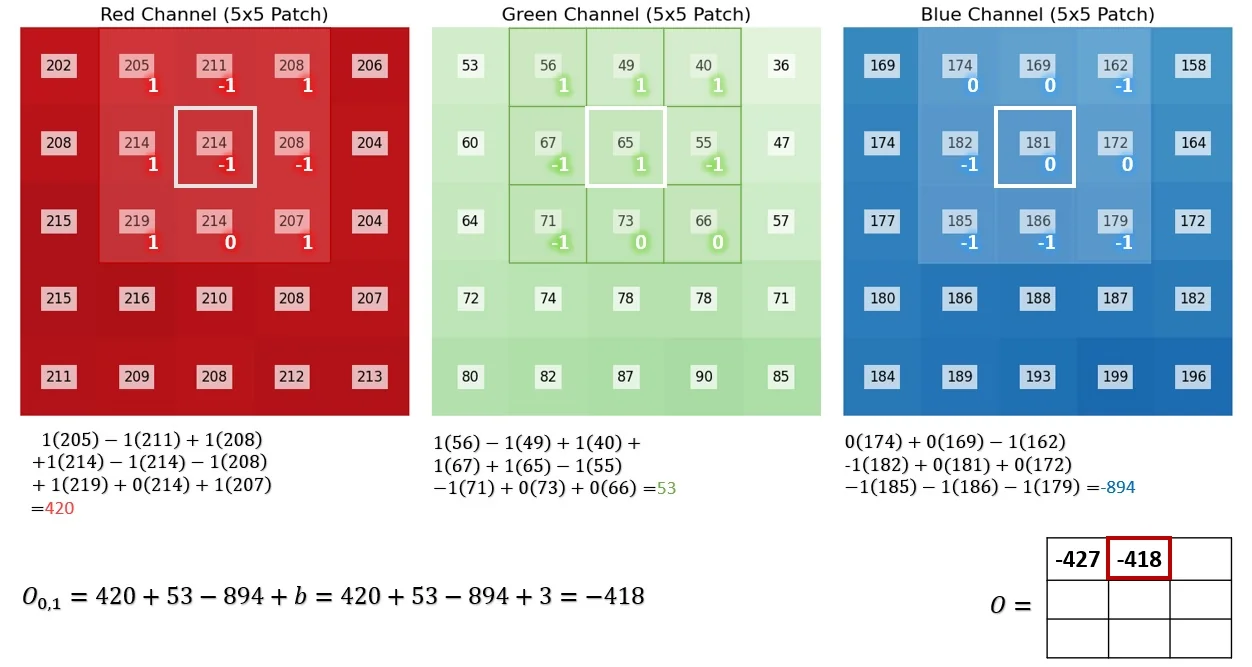
After computing the first output pixel, the filter slides spatially to the next position, repeating the same process across the entire image.
From Single Filters to Complete Convolutional Layers A full convolutional layer consists of multiple filters, each producing a separate activation map. The number of filters, \( C_{\mbox{out}} \), determines the number of output channels in the resulting feature map: \[ C_{\mbox{out}} \times H' \times W'. \] Each filter detects different spatial patterns, allowing the network to capture diverse features such as edges, textures, or object parts. By stacking multiple layers, we progressively build hierarchical representations of the input.
What Our Example Missed: Padding and Stride Our example demonstrated how a convolutional filter processes an image patch, but real-world applications introduce additional complexities:
- Incomplete Coverage of the Image: We only applied convolution to a limited region. In practice, the filter moves across the entire image, computing feature responses at each location.
- Handling Image Borders – Padding: Convolution reduces spatial dimensions unless padding is added around the image. Padding ensures that feature extraction extends to edge pixels and helps control output size.
- Stride – Controlling Spatial Resolution: We assumed a step size of 1 when sliding the filter. Using a larger step size (stride) allows for downsampling, reducing spatial dimensions while preserving depth, helping in mitigation of computational cost.
Are Kernel Values Restricted? Unlike fixed edge detection filters (e.g., Sobel), the values in convolutional kernels are not predefined—they are learned during training. Filters evolve to capture useful features depending on the task. While no strict range constraints exist, regularization techniques such as weight decay help prevent extreme values, improving stability and generalization.
Negative and Large Output Values Standard image pixels range from \(0\) to \(255\), but convolution outputs can have negative values or exceed this range. This is not an issue because convolutional layers produce feature maps, not direct images. Although this isn’t an issue, neural networks sometimes keep these values in check through usage of techniques such as ’Batch Normalization’ that stabilize activations, greatly improving training efficiency.
In the rest of this lecture, we will explore these topics in depth, ensuring a complete understanding of how convolutional layers operate in modern neural networks.
7.3.3 Multiple Filters and Output Channels
A convolutional layer can apply multiple filters, where each filter extracts a different feature from the input. The number of filters determines the number of output channels.
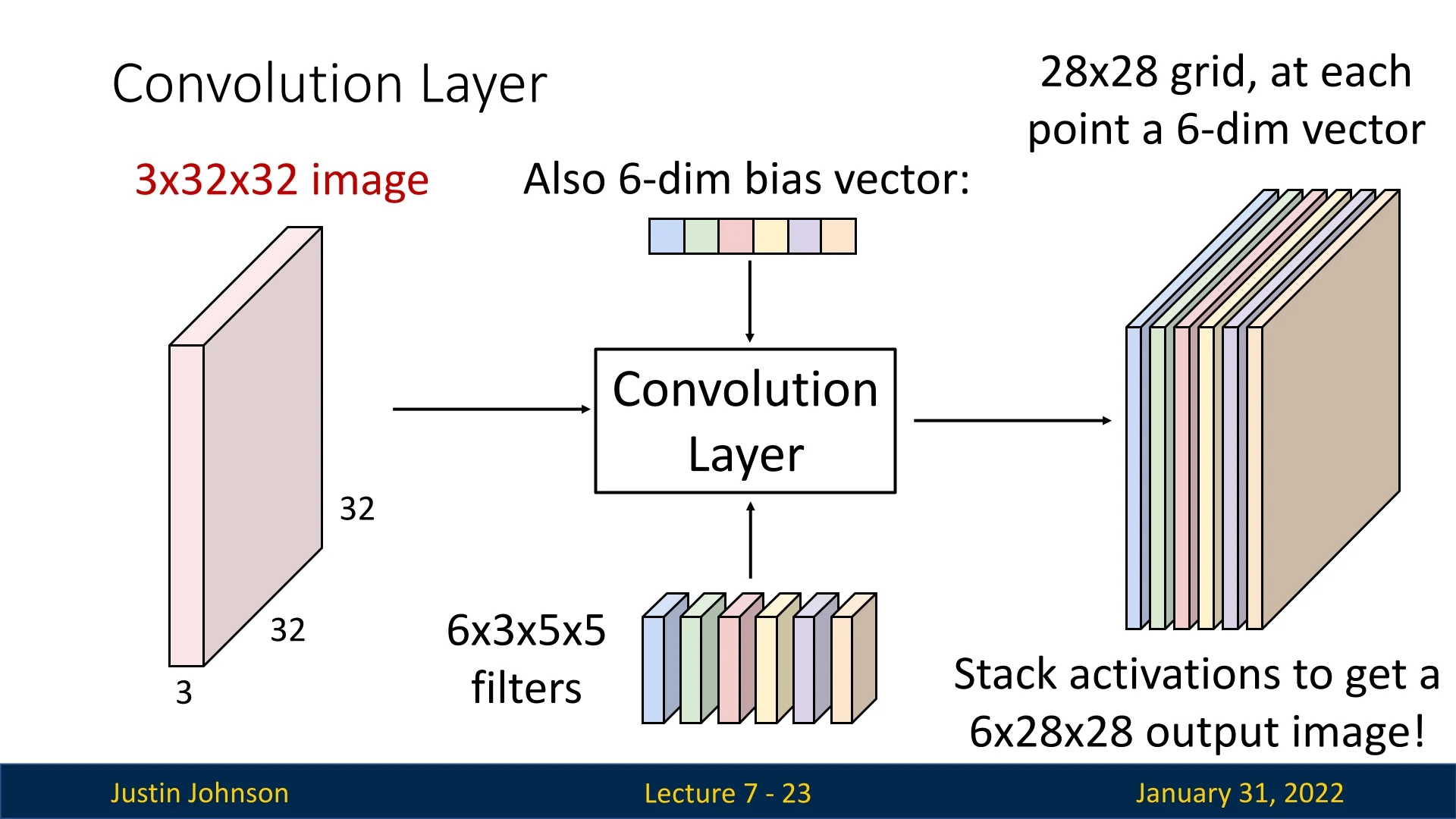
For example, if we apply 6 filters, each of size \( 3 \times 5 \times 5 \), to a \( 3 \times 32 \times 32 \) input image, the output consists of 6 activation maps, each of size \( 1 \times 28 \times 28 \). These maps can be stacked to form an output tensor of shape: \( 6 \times 28 \times 28.\)
7.3.4 Two Interpretations of Convolutional Outputs
The output of a convolutional layer can be viewed in two equivalent ways:
- 1.
- Stack of 2D Feature Maps: Each filter produces one activation map, so stacking all \(C_{\mbox{out}}\) maps yields a \((C_{\mbox{out}} \times H' \times W')\) volume.
- 2.
- Grid of Feature Vectors: Each spatial position \((h,w)\) in the output corresponds to a \(C_{\mbox{out}}\)-dimensional feature vector, representing learned features at approximately (convolutions without padding can reduce the spatial dim of the output tensor a bit) that location in the input tensor.
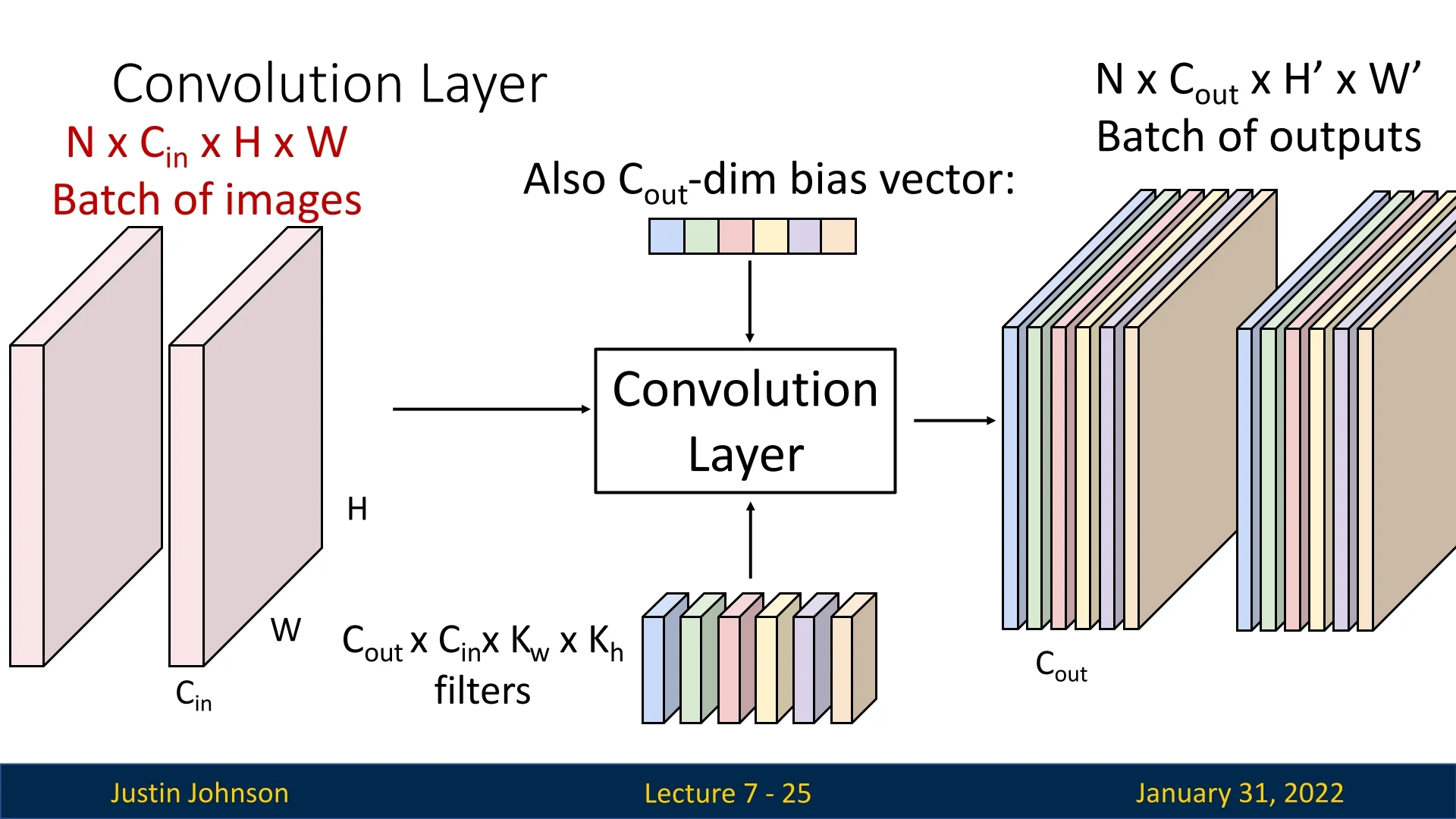
7.3.5 Batch Processing with Convolutional Layers
In practice, convolutional layers process batches of images. If we have a batch of \(N\) input images, each of shape \(C_{\mbox{in}} \times H \times W\), then the input tensor has shape: \[ N \times C_{\mbox{in}} \times H \times W. \] The corresponding output tensor has shape: \[ N \times C_{\mbox{out}} \times H' \times W'. \]
7.5 Building Convolutional Neural Networks
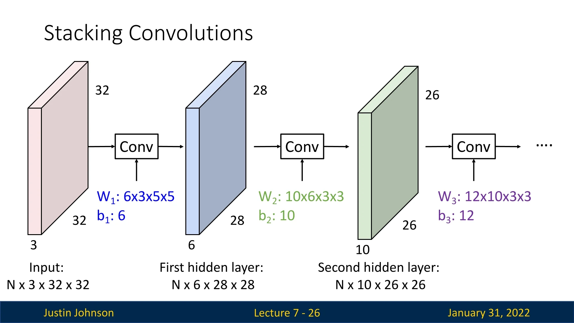
7.4.1 Stacking Convolutional Layers
With convolutional layers, we can construct a new type of neural network by stacking multiple convolutions sequentially. Unlike fully connected layers, where each neuron connects to every input feature, convolutional layers operate locally, extracting spatial features at each step.
The filters in convolutional layers are learned throughout the training process. They adjust dynamically to capture features useful for minimizing the network’s loss, just like the weights in fully connected layers. The output feature map after each convolution has:
- \( C_{\mbox{out}} \) channels (determined by the number of filters in that layer),
- A height \( H' \) and width \( W' \), which may differ from the input dimensions \( H \) and \( W \), depending on the use of padding and strides.
A common architectural pattern in convolutional networks is to reduce spatial dimensions while increasing the number of channels. The rationale for this is:
- Each channel can be seen as a learned feature representation, abstracting spatial patterns across layers.
- Reducing spatial dimensions while increasing channels allows the network to capture high-level patterns, moving from local details (e.g., edges) to global structures (e.g., entire objects).
- It allows neurons in deeper layers to gather information from a progressively larger region of the input, effectively expanding their receptive field. As we stack more convolutional and pooling layers, each neuron becomes responsive to a wider portion of the original image, enabling the network to capture increasingly large-scale structures (e.g., recognizing an entire cat’s face rather than just its whiskers)—a concept we will formalize later when discussing receptive fields.
7.4.2 Adding Fully Connected Layers for Classification
After passing through several convolutional layers, the output is a multi-channel feature representation of the input. To use this representation for classification or regression tasks, we typically:
- Flatten the feature maps into a 1D vector,
- Pass the vector through a fully connected (MLP) layer,
- Use a SoftMax activation (for classification).
This structure allows convolutional layers to act as feature extractors, and the final fully connected layers to perform decision-making based on the extracted features.
7.4.3 The Need for Non-Linearity
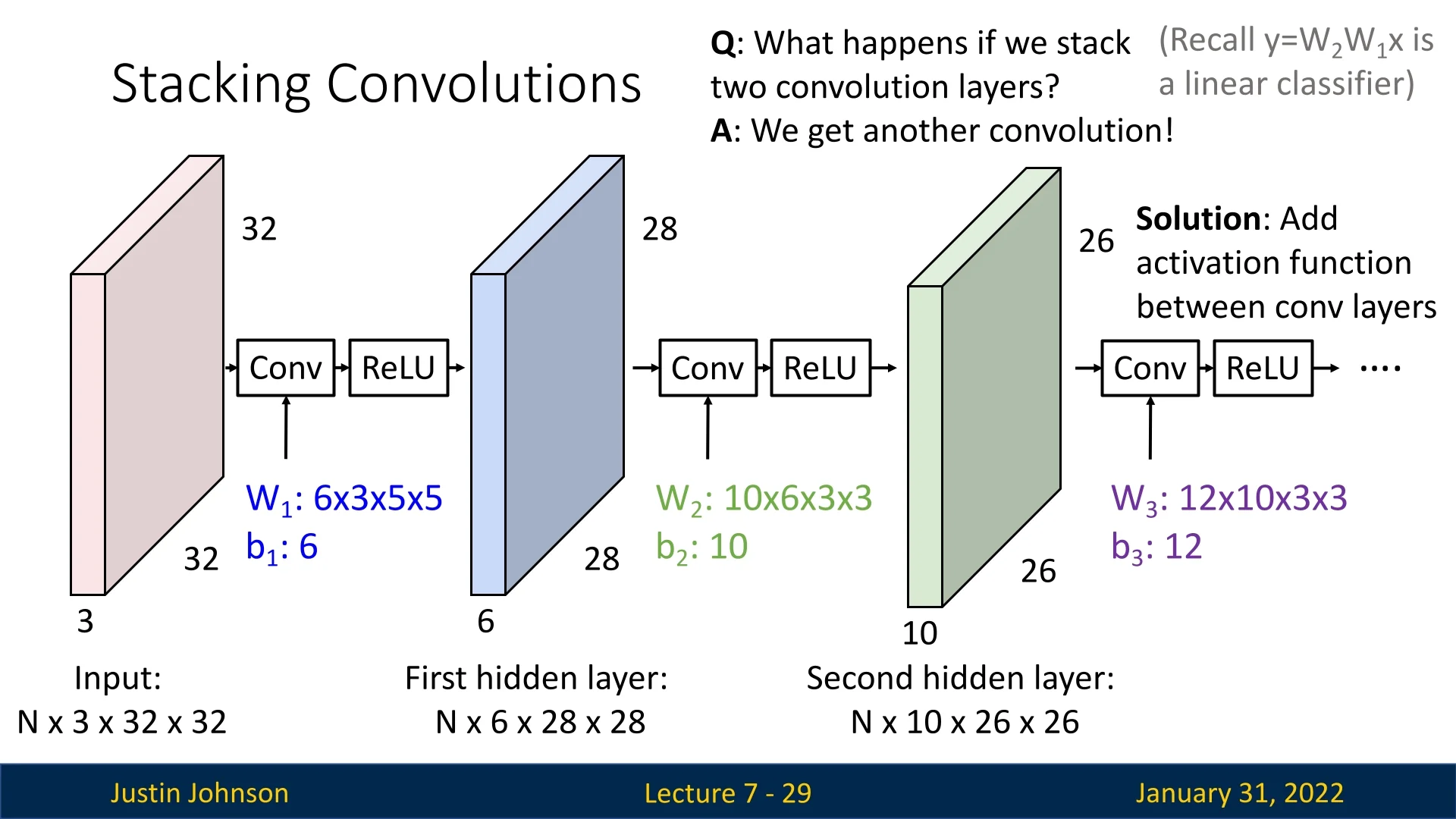
A major issue arises when stacking convolutional layers directly on top of each other: convolution itself is a linear operation. Recall from basic neural network theory that a sequence of linear transformations can always be reduced to a single linear transformation, meaning a network composed purely of stacked convolutional layers has limited expressive power.
Mathematically, consider a network with two convolutional layers: \[ X \xrightarrow {\mbox{Conv}_1} W_1 X \xrightarrow {\mbox{Conv}_2} W_2 W_1 X. \] Since both transformations are linear, the entire operation reduces to a single matrix multiplication. This is analogous to a multi-layer perceptron (MLP) without activation functions, which collapses into a single-layer network, greatly limiting its representational capacity.
The solution is to introduce non-linearity after each convolution. This is typically done using ReLU (Rectified Linear Unit) activations, which apply an element-wise transformation: \[ f(x) = \max (0, x). \] ReLU allows the network to model complex relationships by breaking the linearity of stacked layers, significantly increasing representational power.
7.4.4 Summary
- Stacking Convolutions allows deeper networks to learn increasingly abstract features.
- Reducing spatial dimensions while increasing channels helps capture global patterns in images.
- Flattening and adding fully connected layers enables classification and regression tasks.
- Introducing non-linearity between convolutional layers prevents the network from collapsing into a simple linear transformation, significantly enhancing representational capacity.
In the next sections, we will explore additional techniques such as pooling layers and batch normalization, which further improve the efficiency and stability of convolutional networks.
7.6 Controlling Spatial Dimensions in Convolutional Layers
7.5.1 How Convolution Affects Spatial Size
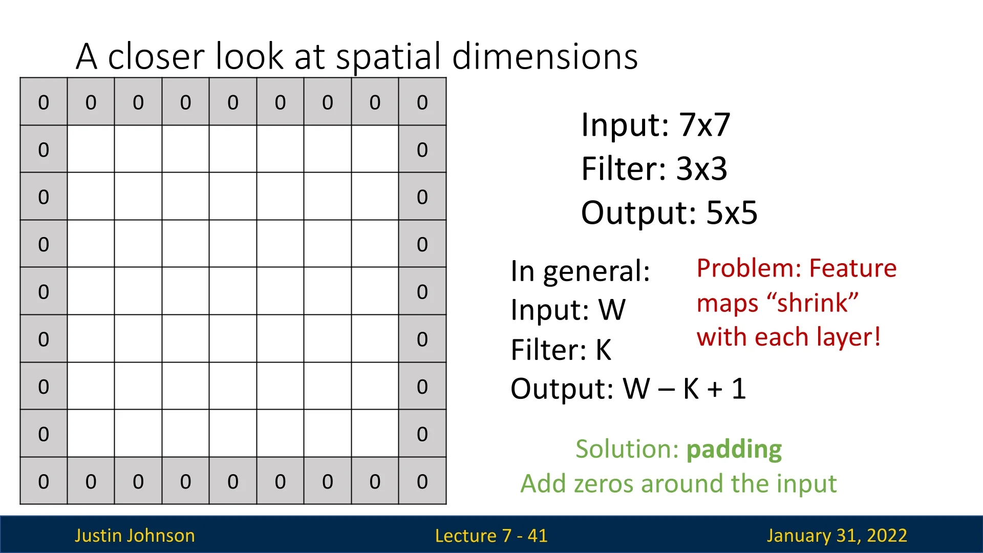
When applying a convolutional filter to an input image, the spatial dimensions of the output shrink. If we start with a square input tensor of spatial size \( W \times W \) and apply a convolutional filter of size \( K \times K \), the output spatial size is given by: \[ W' = W - K + 1. \] For example, when we previously examined a \( 5 \times 5 \) patch of the Lotus image and applied a \( 3 \times 3 \) filter, the resulting feature map had dimensions: \[ 5 - 3 + 1 = 3 \times 3. \] This reduction in spatial size can become problematic as feature maps continue to shrink with deeper layers. If no corrective measures are taken, images may spatially collapse to an unrecognizable form, limiting the depth of our network.
7.5.2 Mitigating Shrinking Feature Maps: Padding
A common solution to prevent excessive spatial shrinkage is padding, where extra pixels are added around the borders of the input image before applying convolution. The most widely used approach is zero-padding, where padding pixels are filled with zeros. More advanced techniques, such as replication padding (copying the values of edge pixels) or reflection padding (mirroring the border values), are sometimes used in practice as well.
Choosing the Padding Size Padding introduces a new hyperparameter, \( P \), which determines how many pixels are added to the borders of the input. A commonly used setting is: \[ P = \frac {K - 1}{2}. \] This choice ensures that the output retains the same spatial dimensions as the input: \[ W' = W - K + 1 + 2P. \] For instance, using a \( 3 \times 3 \) filter with \( P = 1 \) ensures that a \( W \times W \) input produces a \( W \times W \) output. This technique, known as same padding, is widely used in deep convolutional architectures.
Preserving Border Information with Padding Another crucial role of padding is ensuring that the information at the borders of the image is not washed away as convolutional layers stack deeper in a network. Without padding, pixels near the borders of an image are involved in fewer computations than those in the center, leading to a loss of information at the edges. By adding padding, we allow convolutional filters to access meaningful contextual information even for edge pixels, improving feature extraction and preventing a bias toward central regions.
This effect is particularly relevant in tasks such as:
- Object Detection: Key features of an object may appear near the image borders, and padding ensures these features are processed adequately.
- Medical Imaging: In scans such as MRIs or X-rays, abnormalities may be located near the periphery. Padding helps ensure these regions receive equal importance.
- Segmentation Tasks: When performing image segmentation, retaining spatial consistency across the entire image is essential. Padding prevents distortions that could affect segmentation accuracy near the edges.
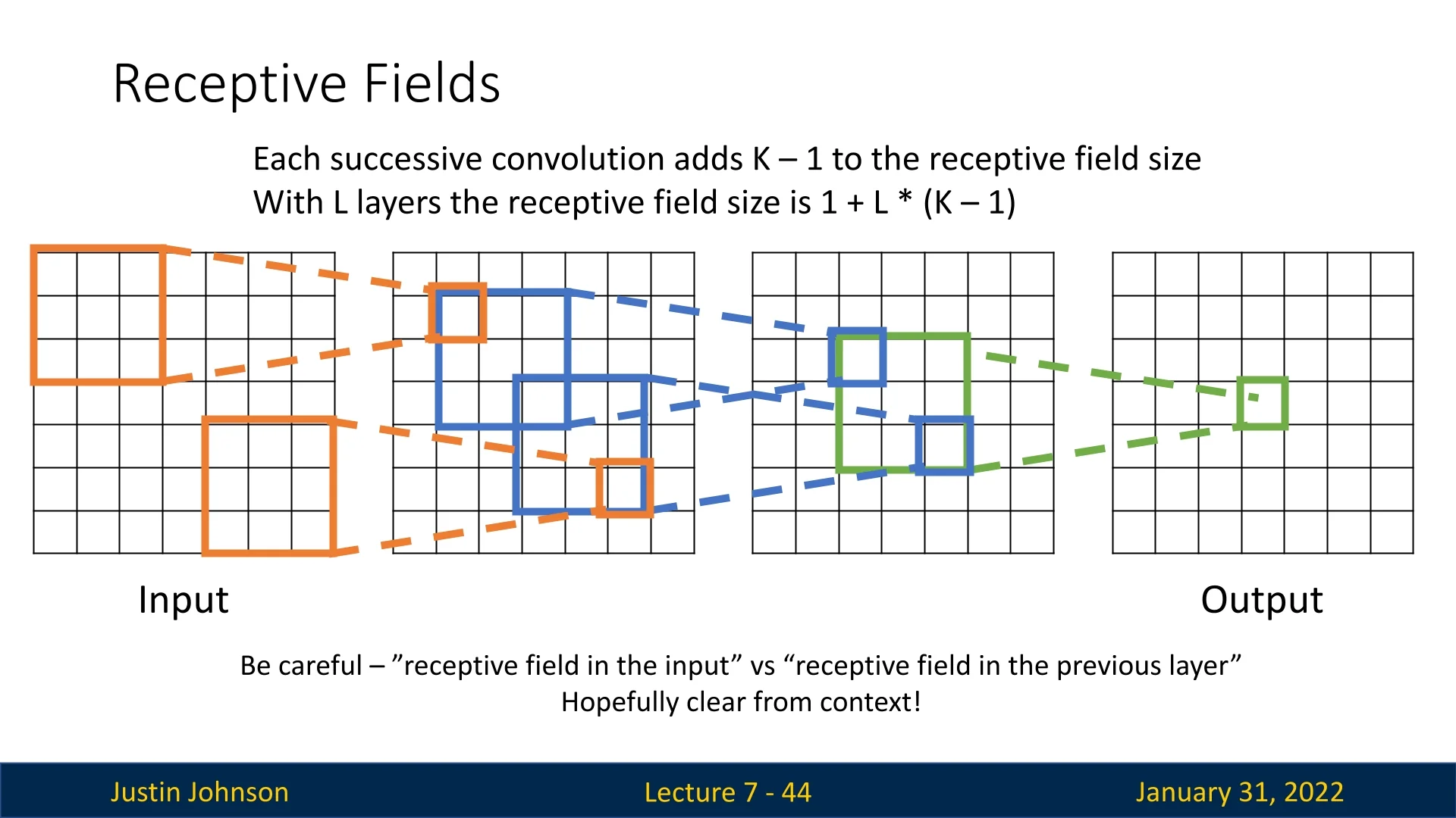
7.5.3 Receptive Fields: Understanding What Each Pixel Sees
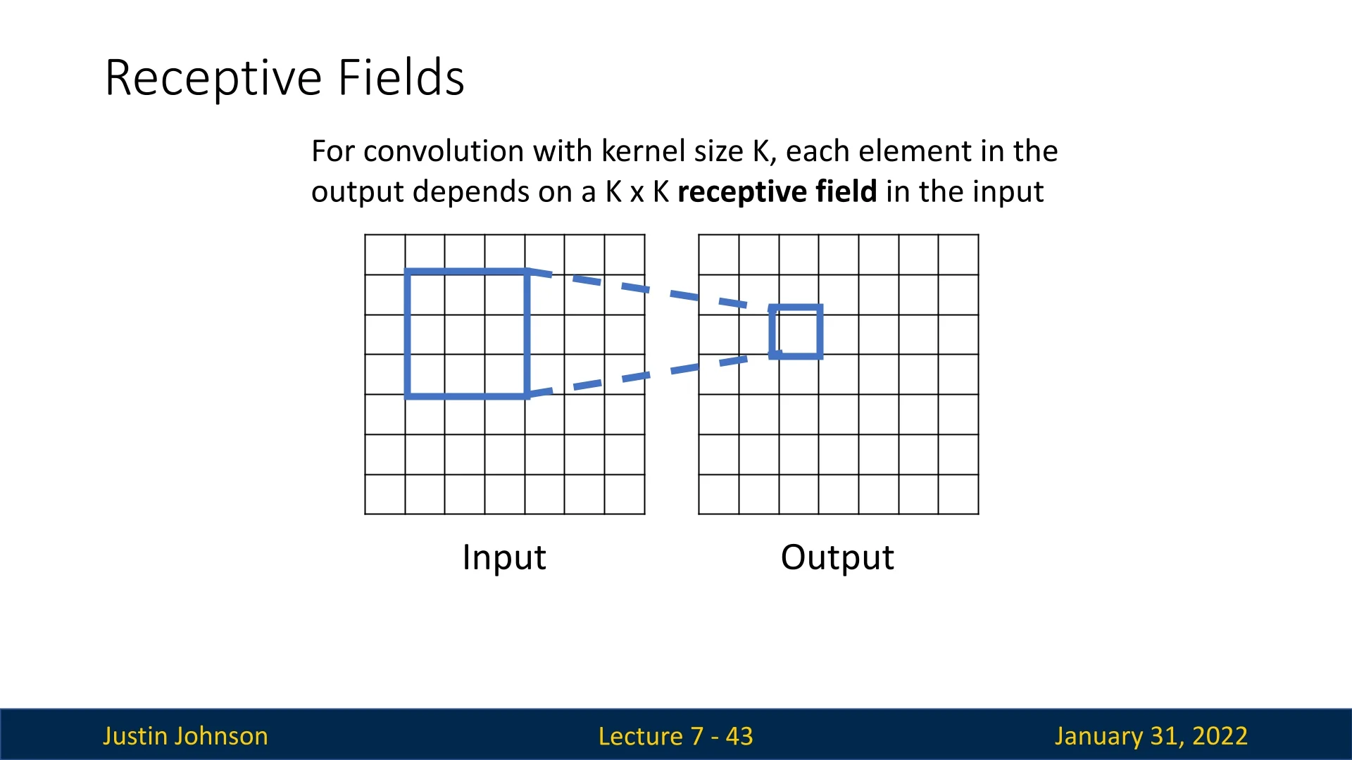
Another way to analyze convolutional networks is by considering the receptive field of each output pixel. The receptive field of an output pixel represents the region in the original input that influenced its value.
Each convolution with a filter of spatial size \( K \times K \) expands the receptive field. With \( L \) convolutional layers, each having a \( K \times K \) filter, the receptive field size can be computed as: \[ \mbox{Receptive Field} = 1 + L \cdot (K - 1). \]
The Problem of Limited Receptive Field Growth
For deep networks, we want each output pixel to have access to a large portion of the original image. However, small kernels (e.g., \(3 \times 3\)) grow the receptive field slowly. Consider a \( 1024 \times 1024 \) image processed with a network using \( 3 \times 3 \) filters. We would need hundreds of layers before each output pixel “sees” the entire image.
Hence, we need to perform a more aggressive downsampling along the neural network. Some of the tools we can use for that purpose are strides and pooling layers. We’ll now cover both of these tools, starting with strides. As pooling layers are a different type of layer in the neural network, we’ll touch them after finishing with convolutions first.
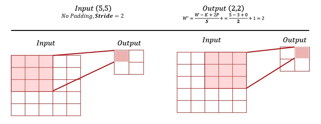
7.5.4 Controlling Spatial Reduction with Strides
Stride is another technique for managing spatial dimensions in convolutional networks. Instead of moving the filter one pixel at a time, we can define a stride \( S \), which determines how many pixels the filter shifts per step. Increasing the stride results in downsampling, reducing the output’s spatial dimensions: \[ W' = \frac {W - K + 2P}{S} + 1. \]
7.7 Understanding What Convolutional Filters Learn
7.6.1 MLPs vs. CNNs: Learning Spatial Structure
Traditional multilayer perceptrons (MLPs) learn weights for the entire image at once, often ignoring spatial structure. In contrast, convolutional neural networks (CNNs) learn filters that operate on small, localized patches, progressively building up more complex representations. This hierarchical feature extraction is key to CNNs’ ability to recognize objects and textures efficiently.
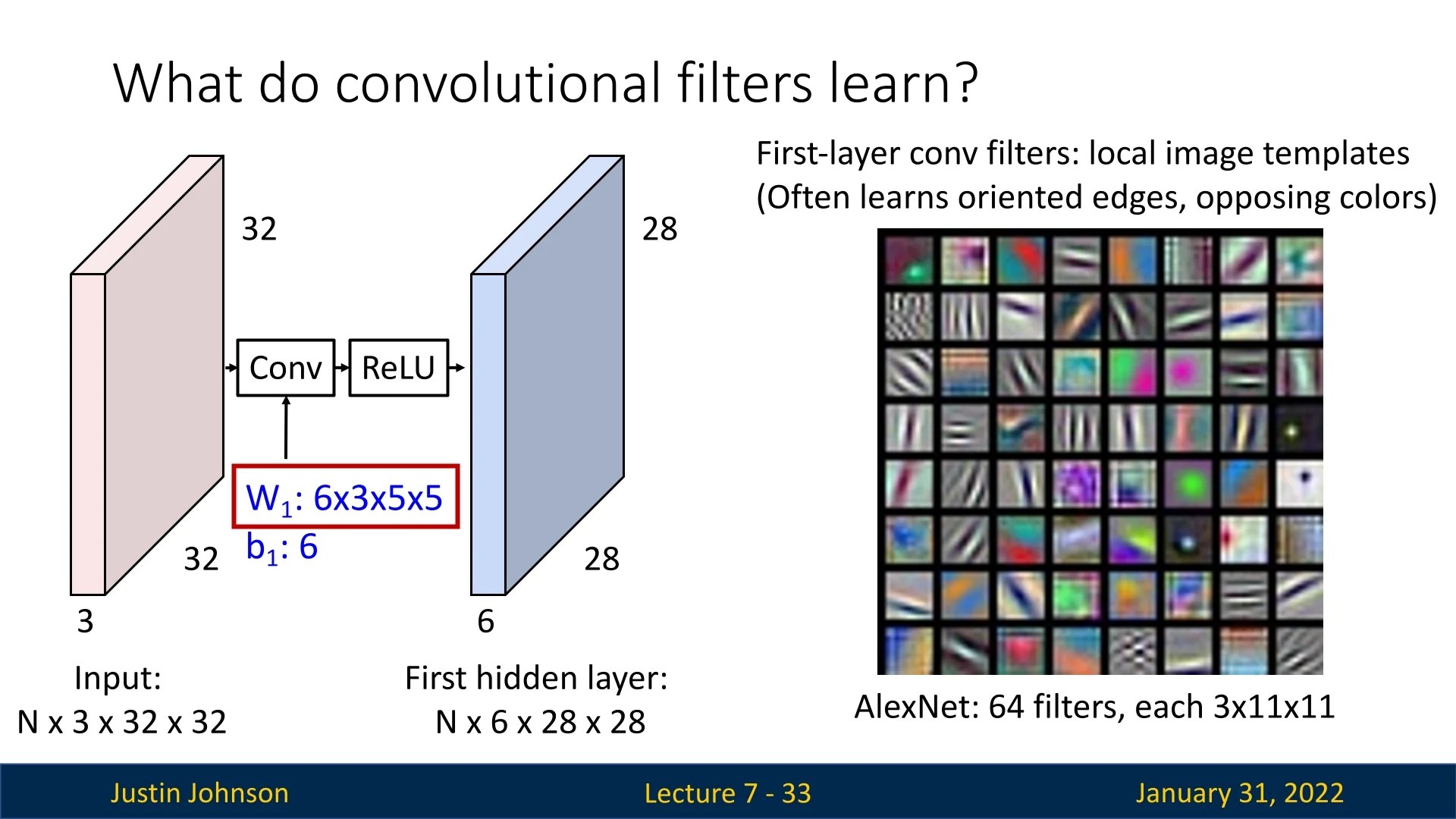
7.6.2 Learning Local Features: The First Layer
The first convolutional layer specializes in detecting fundamental image patterns:
- Local Receptive Fields: Each filter “sees” only a small region of the image (e.g., a \( 3 \times 3 \) patch). As a result, first-layer filters typically learn to detect edges, corners, color gradients, and small textures.
- Feature Maps: Each filter produces a feature map, highlighting areas where a learned pattern appears in the image. Strong activations indicate high similarity to the filter (e.g., bright responses for vertical edges).
7.6.3 Building More Complex Patterns in Deeper Layers
As the network deepens, convolutional layers process feature maps instead of raw pixels, enabling hierarchical feature composition. Each successive layer captures increasingly abstract patterns by integrating information from a growing receptive field.
Hierarchical Learning via Composition
- Early layers: Detect simple edges, gradients, and textures.
- Mid-layers: Combine early features into complex structures like shapes and object parts.
- Deepest layers: Recognize high-level semantic patterns, forming complete object representations.
Deeper networks enhance representational capacity by progressively composing features, transforming raw pixel data into hierarchical object representations. Each layer refines and abstracts information from previous layers, enabling more complex feature extraction. Empirical evidence, including visualization methods like DeepDream, confirms that deeper layers capture high-level semantic concepts. Modern architectures such as ResNets and DenseNets demonstrate that increased depth, when properly managed, improves feature learning and overall model performance.
7.8 Parameters and Computational Complexity in Convolutional Networks
Thus far, we have examined how convolutional layers operate, but an equally important consideration is their computational cost and learnable parameters. Unlike fully connected layers, it’s intuitive that convolutional layers significantly reduce the number of parameters, but what about computational operations?
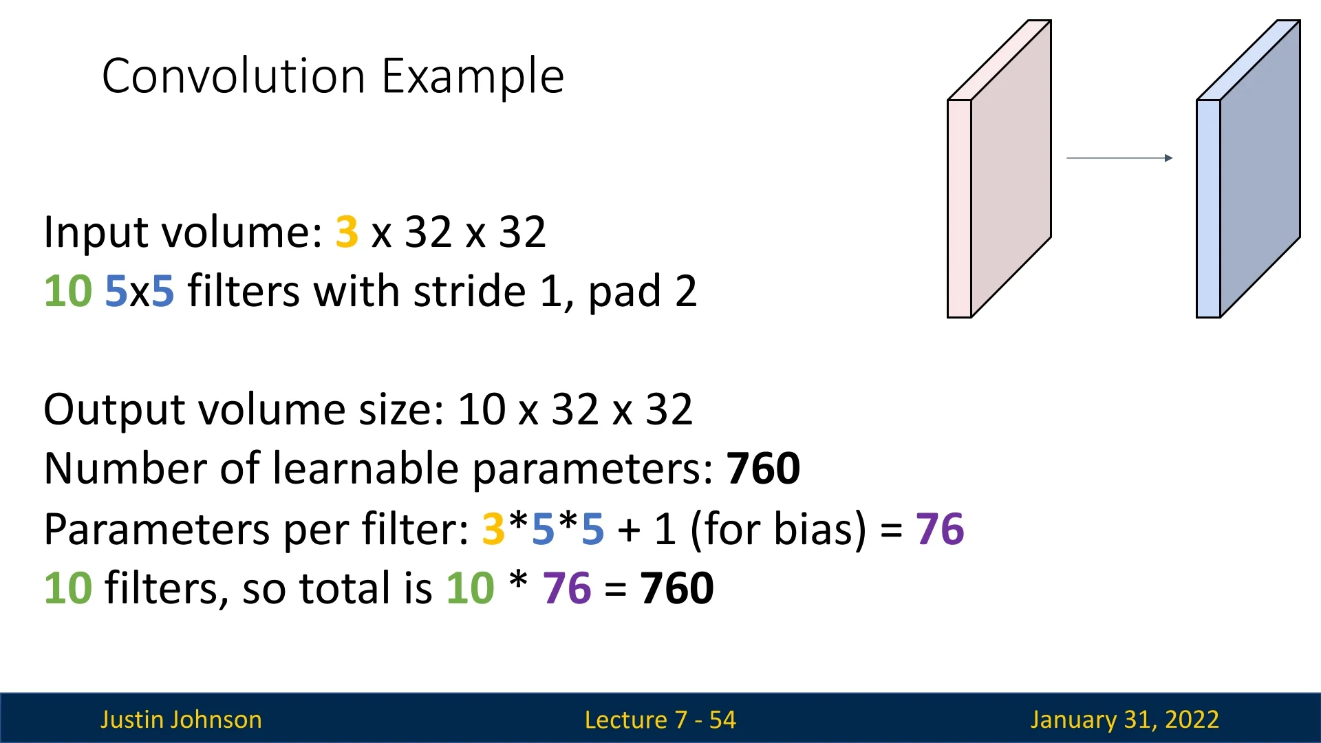
7.7.1 Example: Convolutional Layer Setup
To understand these calculations, consider a single convolutional layer with the following configuration:
- Input volume: \(3 \times 32 \times 32\) (an RGB image with height 32, width 32, and 3 channels).
- Number of filters: 10.
- Filter size: \(3 \times 5 \times 5\).
- Stride: 1.
- Padding: Same padding (\(P = 2\)), preserving spatial dimensions.
7.7.2 Output Volume Calculation
With same padding and stride 1, the spatial dimensions remain: \[ H' = W' = \frac {32 + 2(2) - 5}{1} + 1 = 32. \] Since we have 10 filters, the final output volume is: \[ 10 \times 32 \times 32. \]
7.7.3 Number of Learnable Parameters
Each filter consists of \(3 \times 5 \times 5 = 75\) weights, plus one bias parameter: \[ \mbox{Parameters per filter} = 75 + 1 = 76. \] With 10 filters in the layer: \[ \mbox{Total parameters} = 76 \times 10 = 760. \] This is a significant reduction compared to fully connected layers, where each neuron connects to all input elements.
7.7.4 Multiply-Accumulate Operations (MACs)
The computational cost of a convolutional layer is typically measured in Multiply-Accumulate Operations (MACs), named after their two-step process: multiplying two values and accumulating the result into a running sum. This operation is fundamental in digital signal processing (DSP) and neural network computations, as it efficiently performs weighted summations required for convolutions.
MACs Calculation: The total number of positions in the output volume is: \[ 10 \times 32 \times 32 = 10,240. \] Each spatial position is computed via a dot product between the filter and the corresponding input region, requiring: \[ 3 \times 5 \times 5 = 75 \] MACs per position. Thus, the total number of MACs for the layer is: \[ 75 \times 10,240 = 768,000. \]
7.7.5 MACs and FLOPs
In computational performance metrics, MACs are often translated into Floating-Point Operations (FLOPs). The definition of FLOPs varies depending on hardware:
- Some systems count each MAC as 2 FLOPs (one multiply + one add).
- Others treat a fused MAC as a single FLOP.
Thus, this layer requires:
- \(768,000\) FLOPs (if MACs are counted as one FLOP).
- \(1,536,000\) FLOPs (if each MAC counts as two FLOPs).
7.7.6 Why Multiply-Add Operations (MACs) Matter
MACs provide a key measure of a neural network’s efficiency:
- Computational Cost: The fewer MACs, the faster the network runs, making inference more efficient.
- Design Considerations: Balancing accuracy and computational cost is crucial, and MACs provide a key metric for optimizing architectures.
Even though convolutional networks use fewer parameters than fully connected networks, their computational cost (measured in MACs) can be high, necessitating careful architecture design.
Enrichment 7.8.7: Backpropagation for Convolutional Neural Networks
This enrichment section is adapted from the Medium article by Pavithra Solai [599], providing a clear illustration of backpropagation in convolutional layers.
Key Idea: Convolution as a Graph Node In a computational graph, each convolutional layer receives an upstream gradient \(\frac {dL}{dO}\), where \(O\) is the output of the convolution: \[ O = X \circledast F, \] with \(X\) denoting the input tensor (patch) and \(F\) the convolution filter.
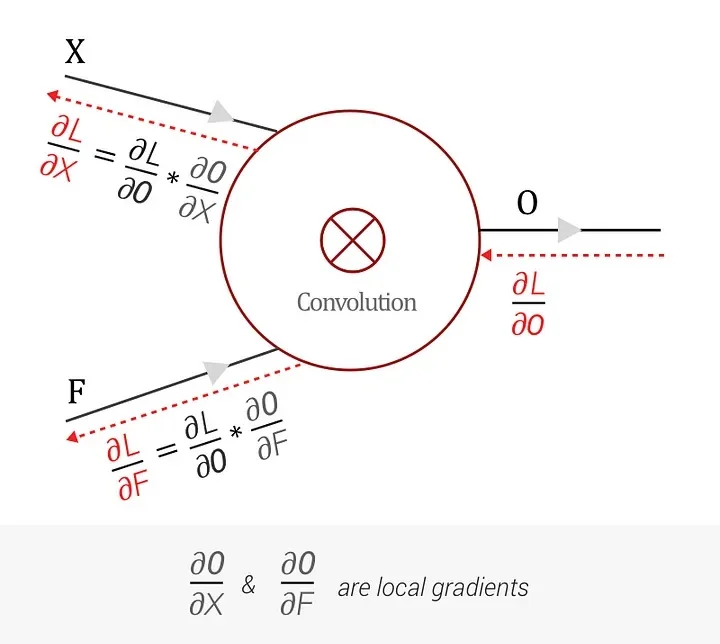
Using the chain rule, we can write: \[ \frac {dL}{dX} = \frac {dL}{dO} \times \frac {dO}{dX}, \quad \frac {dL}{dF} = \frac {dL}{dO} \times \frac {dO}{dF}, \] where \(\tfrac {dO}{dX}\) and \(\tfrac {dO}{dF}\) are the local gradients from the convolution operation, and \(\tfrac {dL}{dO}\) is the upstream gradient arriving from deeper layers.
Computing \(\tfrac {dO}{dF}\) Consider a \((3\times 3)\) input patch \(X\) and a \((2\times 2)\) filter \(F\):
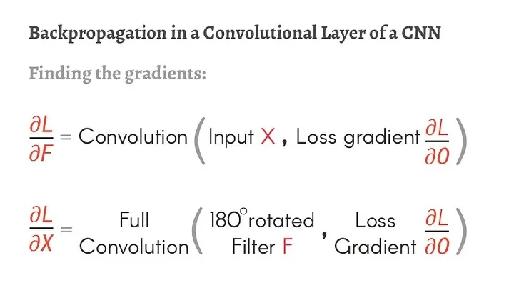
\[ X = \begin {bmatrix} X_{11} & X_{12} & X_{13}\\ X_{21} & X_{22} & X_{23}\\ X_{31} & X_{32} & X_{33} \end {bmatrix},\quad F = \begin {bmatrix} F_{11} & F_{12}\\ F_{21} & F_{22} \end {bmatrix}. \] When convolved, the first element \(O_{11}\) is: \[ O_{11} = X_{11}F_{11} + X_{12}F_{12} + X_{21}F_{21} + X_{22}F_{22}. \] Taking derivatives: \[ \tfrac {\partial O_{11}}{\partial F_{11}} = X_{11},\quad \tfrac {\partial O_{11}}{\partial F_{12}} = X_{12},\quad \tfrac {\partial O_{11}}{\partial F_{21}} = X_{21},\quad \tfrac {\partial O_{11}}{\partial F_{22}} = X_{22}. \] Repeating for \(O_{12},O_{21},O_{22}\) yields similar terms. Thus, \(\tfrac {dL}{dF_i}\) arises from summing elementwise gradients over all spatial locations: \[ \tfrac {dL}{dF_i} = \sum _{k=1}^{M} \tfrac {dL}{dO_k} \;\tfrac {\partial O_k}{\partial F_i}. \] Effectively, \(\tfrac {dL}{dF}\) can be interpreted as a convolution of \(X\) with \(\tfrac {dL}{dO}\).
Computing \(\tfrac {dL}{dX}\) A similar argument applies to \(\tfrac {dL}{dX}\). In fact, \[ \tfrac {dL}{dX} = F^\star \;\circledast \; \tfrac {dL}{dO}, \] where \(F^\star \) is a 180-degree rotation of the filter \(F\).
Full details and visual examples can be found in [599], which provide additional insights into the math and coding approach for convolutional backprop.
Enrichment 7.9: Parameter Sharing in Convolutional Neural Networks
Convolutional Neural Networks (CNNs) leverage parameter sharing to drastically reduce the number of parameters while maintaining high representational power. The key assumption behind parameter sharing is that features learned at one spatial location are also useful at other locations, which is particularly beneficial for images with translational invariance.
Enrichment 7.9.1: Parameter Sharing in CNNs vs. MLPs
Unlike Multilayer Perceptrons (MLPs), which assign independent weights to each input neuron, CNNs apply the same set of weights across different spatial locations. In an MLP, each layer has a fully connected structure, leading to a number of parameters that scales quadratically with input size. In contrast, CNNs use convolutional filters that slide across the image, sharing parameters across spatial positions. This difference enables CNNs to efficiently learn spatial hierarchies while significantly reducing computational complexity.
Enrichment 7.9.2: Motivation for Parameter Sharing
Parameter sharing is motivated by several key advantages:
- Reducing Parameters: Instead of learning independent weights for every neuron, CNNs share a common set of weights across the spatial dimensions. This significantly reduces the number of parameters and makes training more efficient.
- Translational Invariance: If detecting a specific feature (e.g., an edge, a texture) is useful in one part of the image, it should also be useful elsewhere. This property aligns well with the structure of natural images.
- Learning Efficient Representations: By sharing parameters across spatial locations, the model learns generalized feature detectors that work across an image rather than overfitting to specific pixel locations.
Enrichment 7.9.3: How Parameter Sharing Works
The neurons in a convolutional layer are constrained to use the same set of weights and biases across different spatial locations.
- Mathematically, for an input image \( X \), a convolutional kernel \( W \), and a bias term \( b \), the convolution operation at location \( (i,j) \) is computed as: \begin {equation} Y_{ij} = \sum _{m} \sum _{n} W_{mn} X_{i+m, j+n} + b. \end {equation}
- The same filter \( W \) is applied across all positions, ensuring that the network learns spatially invariant representations.
Enrichment 7.9.4: When Does Parameter Sharing Not Make Complete Sense?
While parameter sharing is a powerful technique, there are scenarios where it may not be fully appropriate:
- Structured Inputs: If the input images have a specific centered structure, different spatial locations may require distinct features. For example, in datasets where objects (e.g., faces) are always centered, features extracted from the left and right sides of an image may need to be different.
- Example: Face Recognition: In facial recognition, eyes, noses, and mouths appear in predictable locations. It may be beneficial to learn different filters for different regions (e.g., eye-specific features vs. mouth-specific features), rather than enforcing parameter sharing across all positions. An example: [618].
- Medical Imaging: In medical scans (e.g., MRIs or CT scans), abnormalities may occur at specific spatial locations. Detecting a tumor in a specific organ may require distinct filters tailored to that region rather than using the same features everywhere. An example: [374].
- Autonomous Driving: Road scenes contain structured components such as sky, road, and vehicles, each of which may require specialized filters based on their typical locations in the image.
Enrichment 7.9.5: Alternative Approaches When Parameter Sharing Fails
In cases where parameter sharing is not ideal, alternative architectures can be used:
Enrichment 7.9.5.1: Locally-Connected Layers
Unlike standard convolutional layers, locally-connected layers do not share weights across spatial positions. Instead, each neuron in the layer learns a unique set of weights, allowing the network to specialize different feature detectors for different spatial regions. This is particularly useful when spatial position conveys meaning, such as in medical imaging, facial recognition, and structured object recognition.
Enrichment 7.9.5.2: Understanding Locally-Connected Layers
The concept of locally-connected layers extends from convolutional layers but removes the translational invariance constraint. Instead of applying the same filter everywhere, each spatial position has its own learnable filter. Mathematically, this is represented as: \begin {equation} Y_{ij} = \sum _{m} \sum _{n} W_{mn}^{(ij)} X_{i+m, j+n} + b_{ij}, \end {equation} where each weight matrix \( W^{(ij)} \) and bias \( b_{ij} \) is unique to its corresponding spatial position \( (i,j) \). This allows for spatially varying feature extraction.
Enrichment 7.9.5.3: Limitations of Locally-Connected Layers
Despite their advantages, locally-connected layers come with several drawbacks:
- Increased Parameter Count: Unlike convolutional layers, where the same filters are reused, locally-connected layers require separate filters for each spatial position, leading to a substantial increase in parameters.
- Higher Computational Cost: Training and inference become more expensive due to the increased number of independent weights.
- Reduced Generalization: By removing parameter sharing, the model may require more data to learn robust features that generalize well.
While locally-connected layers can be powerful for structured image processing tasks, they are often used selectively in deep learning architectures.
In practice, hybrid models that combine convolutional and locally-connected layers provide a balance between generalization and spatial specificity, and are sometimes used in practice for the particular situations in which full parameter-sharing approach doesn’t make total sense.
Enrichment 7.9.5.4: Hybrid Approaches
Some architectures combine parameter-sharing layers with locally-connected layers to balance generalization and location-specific feature learning. For example, early layers may use standard convolutional layers to learn general features, while later layers may incorporate locally-connected layers to capture region-specific information.
Enrichment 7.9.5.5: A Glimpse at Attention Mechanisms
Another alternative to parameter sharing is self-attention, which dynamically determines how important different regions of an input are to each other. This mechanism, employed in Vision Transformers (ViTs), allows for flexible representation learning beyond the fixed structure of convolutional filters. We will explore self-attention in detail in later chapters.
Parameter sharing is a key ingredient in the success of CNNs, enabling them to generalize effectively while keeping models computationally efficient. However, in cases where spatial locations carry distinct feature importance, alternative approaches such as locally-connected layers or attention mechanisms may be required.
7.10 Special Types of Convolutions: 1x1, 1D, and 3D Convolutions
Beyond standard 2D convolutions, different variations exist to address various computational and structural needs in deep learning models. In this section, we explore 1x1 convolutions for feature adaptation, 1D convolutions for sequential data, and 3D convolutions for volumetric and spatiotemporal processing.
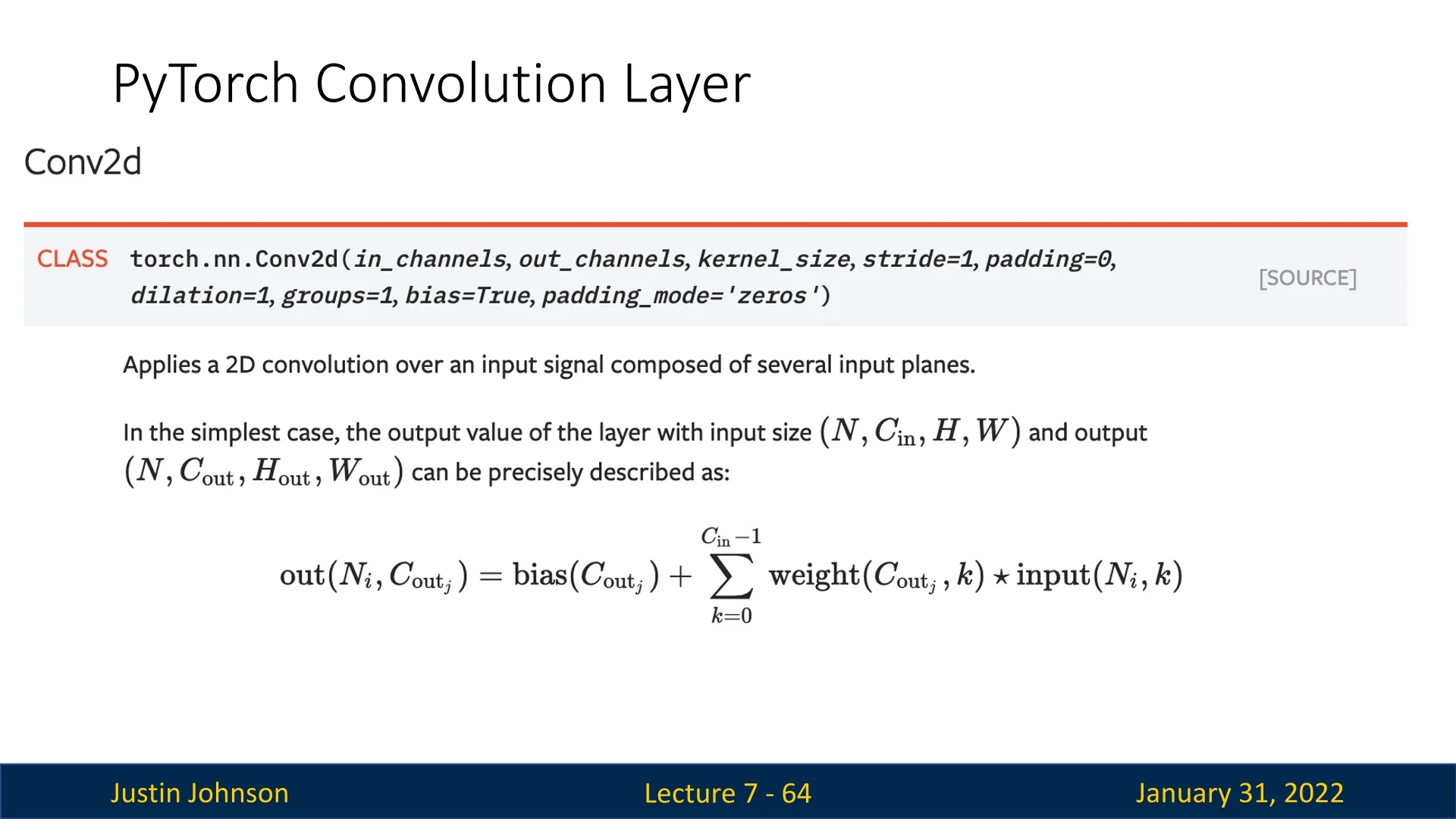
7.8.1 1x1 Convolutions
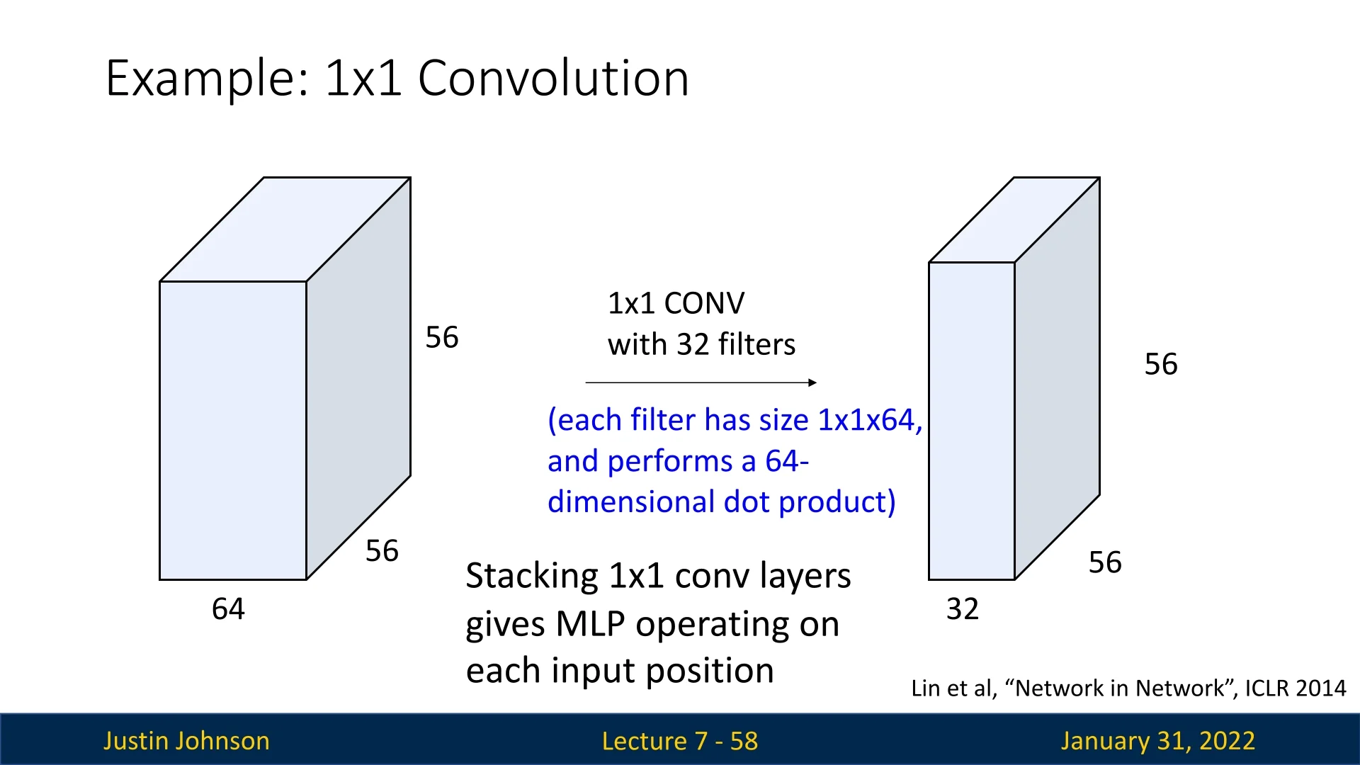
A 1x1 convolution applies a kernel of size \(1 \times 1\), meaning each filter operates on a single spatial position but across all input channels. Unlike traditional convolutions, which aggregate information from neighboring pixels, 1x1 convolutions focus solely on depth-wise transformations.
Dimensionality Reduction and Feature Selection
One common use of 1x1 convolutions is reducing computational complexity. For example, suppose a convolutional layer outputs an activation map of shape \( (N, F, H, W) \), where:
- \( N \) is the batch size,
- \( F \) is the number of input channels,
- \( H, W \) are the spatial dimensions.
If we apply a layer with \( F_1 \) 1x1 filters, the output shape becomes \( (N, F_1, H, W) \), effectively modifying the number of feature channels without altering spatial dimensions.
Efficiency of 1x1 Convolutions as a Bottleneck
A common strategy in modern CNN architectures (e.g., ResNet) is to introduce a 1x1 convolution before (and sometimes after) a more expensive 3x3 convolution, temporarily reducing the number of channels on which the 3x3 operates. This design, often called a bottleneck, lowers both parameter counts and floating-point operations (FLOPs) while preserving representational capacity.
Example: Transforming 256 Channels to 256 Channels with a 3x3 Kernel. Suppose the input has 256 channels of spatial size \(64\times 64\), and we want an output of 256 channels with spatial size \(62\times 62\) (no padding, stride 1).
- 1.
- Direct 3x3 Convolution.
- Parameters: Each of the 256 output channels has \((256 \times 3 \times 3)\) weights plus 1 bias. Total: \[ 256 \times (256 \times 3 \times 3) + 256 \;\approx \; 590{,}080. \]
- FLOPs: The output shape is \(256 \times 62 \times 62\), i.e. \(984{,}064\) output positions. Each position requires \((256 \times 3 \times 3) = 2304\) multiply-adds, giving approximately \[ 984{,}064 \times 2304 \;\approx \; 2.27 \times 10^9 \mbox{ MACs}. \]
- 2.
- Bottleneck: 1x1 Then 3x3. First use a 1x1 convolution to reduce the
input from 256 channels down to 64, apply the 3x3 on these 64 channels,
and then restore 256 channels if needed.
- 1x1 stage (256 \(\to \) 64): \((256 \times 64)\) weights plus 64 biases \(\Rightarrow \sim 16{,}448\) parameters. The output is \((64 \times 64 \times 64)\) (i.e. \(64\) channels, each \(64\times 64\)). This step requires \(\sim 64 \times 64\) spatial positions \(\times (256 \times 64)\) MACs \(\approx 67\times 10^6\) MACs.
- 3x3 stage (64 \(\to \) 256): \((64 \times 256 \times 3 \times 3) + 256\) parameters \(\approx 147{,}712\). The final output shape is \((256 \times 62 \times 62)\). Each of the \(984{,}064\) positions requires \((64 \times 3 \times 3)=576\) MACs, totaling \(\sim 567\times 10^6\) MACs.
- Totals for 1x1 + 3x3: \[ \mbox{Params} = 16{,}384 + 64 + 147{,}456 + 256 \;=\;164{,}160, \qquad \mbox{MACs} \approx 67\times 10^6 + 567\times 10^6 = 634\times 10^6. \]
- Parameters: Direct 3x3 uses \(\sim 590{,}080\) parameters versus \(\sim 164{,}160\) in the bottleneck approach—a 3.6\(\times \) reduction.
- FLOPs: Direct 3x3 costs \(\sim 2.27\times 10^9\) MACs vs. \(\sim 0.63\times 10^9\) for the 1x1+3x3 route—again around a 3.6\(\times \) speedup.
Although the bottleneck adds an extra layer (the 1x1 convolution), the combined memory footprint and compute overhead are significantly lower. This allows CNNs to grow deeper—by reducing intermediate channels—without exploding in parameter or FLOP requirements.
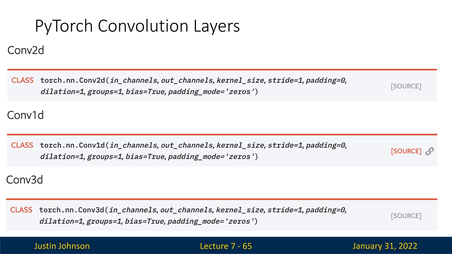
7.8.2 1D Convolutions
1D convolutions operate on sequential data where input dimensions are \( C_{\mbox{in}} \times W \). Filters have shape \( C_{\mbox{out}} \times C_{\mbox{in}} \times K \), where \( K \) is the kernel size.
Numerical Example: 1D Convolution on Multichannel Time Series Data Consider an accelerometer dataset collected from a wearable device, where each row represents acceleration along the \( x, y, z \) axes over time. The input sequence is:
\[ X = \begin {bmatrix} 2 & 3 & 1 & 0 & 4 \\ 1 & 2 & 0 & 1 & 3 \\ 0 & 1 & 2 & 3 & 1 \end {bmatrix} \] with dimensions \( 3 \times 5 \) (three input channels, five time steps).
We apply a 1D convolution with:
- A filter of size \( K = 3 \) operating across all input channels.
- Kernel weights: \[ W = \begin {bmatrix} 1 & 0 & -1 \\ -1 & 1 & 0 \\ 0 & -1 & 1 \end {bmatrix} \]
- Zero padding \( P = 0 \).
- Stride \( S = 2 \).
Computing the Output The output size is computed as: \[ W' = \frac {(W - K + 2P)}{S} + 1 = \frac {(5 - 3 + 2 \times 0)}{2} + 1 = \frac {2}{2} + 1 = 1 + 1 = 2. \]
Since the numerator \( (W - K + 2P) = 2 \) is divisible by \( S = 2 \), no flooring is needed. Thus, the final output has shape \( 1 \times 2 \).
Now, computing the convolution while skipping every second step due to \( S=2 \):
1. First step (\( Y_1 \)): Apply the kernel to the first three columns of the input (columns 1-3): \[ Y_1 = (1 \cdot 2) + (0 \cdot 3) + (-1 \cdot 1) + (-1 \cdot 1) + (1 \cdot 2) + (0 \cdot 0) + (0 \cdot 0) + (-1 \cdot 1) + (1 \cdot 2) \] \[ = 2 + 0 - 1 - 1 + 2 + 0 + 0 - 1 + 2 = 3. \]
2. Second step (\( Y_2 \)): Move by \( S=2 \) steps, selecting columns 3-5: \[ Y_2 = (1 \cdot 1) + (0 \cdot 0) + (-1 \cdot 4) + (-1 \cdot 0) + (1 \cdot 1) + (0 \cdot 3) + (0 \cdot 2) + (-1 \cdot 3) + (1 \cdot 1) \] \[ = 1 + 0 - 4 - 0 + 1 + 0 + 0 - 3 + 1 = -4. \]
Thus, the final output is: \[ Y = [3, -4] \] with shape \( 1 \times 2 \).
Applications of 1D Convolutions
- Activity Recognition: Used on accelerometer data to classify human activity (e.g., standing, walking, running).
- Audio Processing: Applied to waveforms for sound classification or speech recognition.
- Financial Time Series: Detects trends and patterns in stock prices or sensor signals.
7.8.3 3D Convolutions
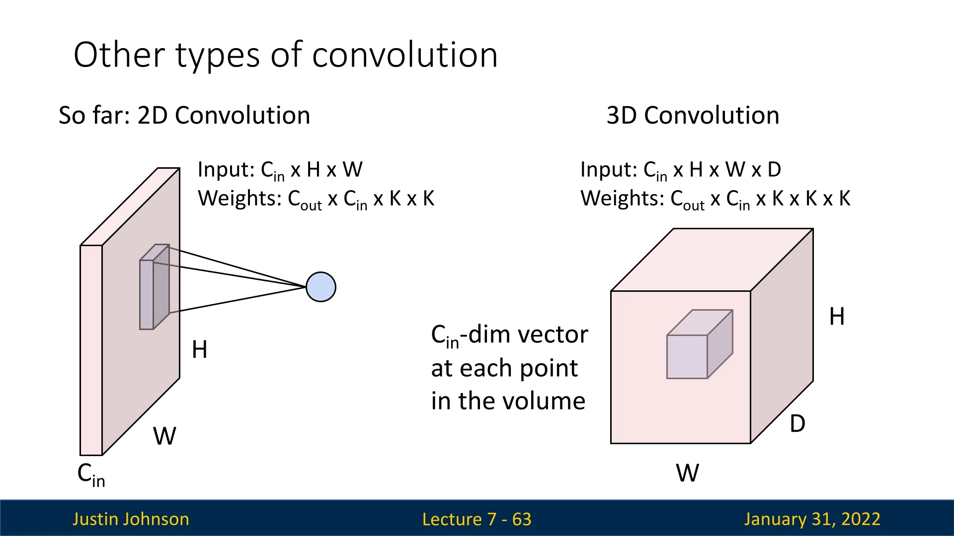
3D convolutions extend 2D convolutions to volumetric data, where input dimensions are \( C_{\mbox{in}} \times H \times W \times D \). Filters have shape \( C_{\mbox{out}} \times C_{\mbox{in}} \times K \times K \times K \).
Numerical Example: 3D Convolution on Volumetric Data Consider a volumetric input (e.g., a single-channel medical scan or short video clip) represented as a 5D tensor: \[ X \in \mathbb {R}^{(N,\, C_{\mbox{in}},\, D_{\mbox{in}},\, H_{\mbox{in}},\, W_{\mbox{in}})} = (1,\, 1,\, 4,\, 4,\, 4), \] where \(N=1\) is the batch size, \(C_{\mbox{in}}=1\) is the number of input channels, and \(D_{\mbox{in}}, H_{\mbox{in}}, W_{\mbox{in}}\) are the spatial depth, height, and width.
We apply a 3D convolution with the following parameters:
- Kernel size \(K = (3,3,3)\).
- Zero padding \(P = 0\).
- Stride \(S = 1\).
- Output channels \(C_{\mbox{out}} = 1\).
Output Size Calculation The output spatial dimensions are given by: \[ O = \left \lfloor \frac {I - K + 2P}{S} \right \rfloor + 1. \] Substituting our values: \[ D_{\mbox{out}} = H_{\mbox{out}} = W_{\mbox{out}} = \left \lfloor \frac {4 - 3 + 0}{1} \right \rfloor + 1 = 2. \] Hence the output tensor has shape: \[ Y \in \mathbb {R}^{(N,\, C_{\mbox{out}},\, D_{\mbox{out}},\, H_{\mbox{out}},\, W_{\mbox{out}})} = (1,\, 1,\, 2,\, 2,\, 2). \]
Input Tensor (Depth Slices) \[ X = \begin {bmatrix} \begin {bmatrix} 1 & -2 & 5 & 2 \\ -1 & 1 & 4 & -3 \\ 1 & 5 & 5 & 2 \\ -1 & -2 & 2 & 2 \end {bmatrix}, \begin {bmatrix} -3 & 0 & -1 & -4 \\ 2 & 0 & -4 & -1 \\ -5 & 4 & 0 & 3 \\ -5 & 5 & 5 & 4 \end {bmatrix}, \begin {bmatrix} -3 & 1 & -2 & 3 \\ -3 & -1 & -3 & 1 \\ -1 & 3 & 1 & -4 \\ -2 & 3 & -4 & 4 \end {bmatrix}, \begin {bmatrix} 3 & 4 & -1 & -4 \\ -2 & 1 & 2 & -3 \\ -5 & -2 & -4 & 2 \\ -2 & -4 & 0 & 0 \end {bmatrix} \end {bmatrix}. \]
Filter Tensor (Kernel) For \(C_{\mbox{out}} = 1\) and \(C_{\mbox{in}} = 1\), the kernel has full shape \[ K \in \mathbb {R}^{(1,\,1,\,3,\,3,\,3)}. \] We can visualize the 3D kernel (depth slices) as: \[ K = \begin {bmatrix} \begin {bmatrix} -2 & 0 & 2 \\ 1 & 3 & -2 \\ -2 & 0 & -2 \end {bmatrix}, \begin {bmatrix} -2 & 2 & 0 \\ 2 & 3 & 3 \\ 2 & 3 & 0 \end {bmatrix}, \begin {bmatrix} -3 & 2 & 1 \\ 1 & -2 & 3 \\ 1 & -2 & -3 \end {bmatrix} \end {bmatrix}. \]
Role of the Input Channel Dimension \(C_{\mbox{in}}\) In this example, \(C_{\mbox{in}}=1\), meaning the convolution integrates purely over spatial dimensions (depth, height, width). In general, for multi-channel inputs such as an RGB video (\(C_{\mbox{in}}=3\)) or multi-modal medical volume (\(C_{\mbox{in}}>1\)), the kernel expands accordingly: \[ K \in \mathbb {R}^{(C_{\mbox{out}},\, C_{\mbox{in}},\, K_D,\, K_H,\, K_W)}. \] At each output position, the convolution sums over all input channels: \[ Y_{c_{\mbox{out}}, d, h, w} = \sum _{c_{\mbox{in}}=0}^{C_{\mbox{in}}-1} \sum _{i=0}^{K_D-1} \sum _{j=0}^{K_H-1} \sum _{k=0}^{K_W-1} X_{c_{\mbox{in}},\, d+i,\, h+j,\, w+k} \, K_{c_{\mbox{out}},\, c_{\mbox{in}},\, i,\, j,\, k}. \] This mechanism fuses cross-channel information—critical, for example, in learning color-motion correlations in video or multi-spectral cues in MRI.
Single-Channel Case (\(C_{\mbox{in}}=C_{\mbox{out}}=1\)) For our numerical example, the channel sum reduces to a single term: \[ Y(d, h, w) = \sum _{i=0}^{2} \sum _{j=0}^{2} \sum _{k=0}^{2} X(d+i, h+j, w+k) \cdot K(i,j,k). \]
Step-by-Step Computation Each output element is the dot product of a \(3\times 3\times 3\) subvolume of \(X\) with the kernel \(K\).
- First output value \(Y(0,0,0)\): \begin {align*} Y(0,0,0) &= \sum _{i=0}^{2}\sum _{j=0}^{2}\sum _{k=0}^{2} X(i,j,k)\,K(i,j,k) \\ &= (-10) + (0) + (-11) = \mathbf {-21}. \end {align*}
- Second value \(Y(0,0,1)\): (shifted one step in width) \[ Y(0,0,1) = \sum _{i,j,k} X(i,j,k+1)\,K(i,j,k) = \mathbf {21}. \]
Final Output Tensor Repeating this process for all valid spatial positions yields: \[ Y = \begin {bmatrix} \begin {bmatrix} -21 & 21 \\ 13 & 28 \end {bmatrix}, \begin {bmatrix} 32 & -61 \\ 17 & -29 \end {bmatrix} \end {bmatrix}. \] Thus the final output tensor has dimensions \(2 \times 2 \times 2\) (or equivalently \(1 \times 1 \times 2 \times 2 \times 2\) including batch and channel).
Applications of 3D Convolutions
- Video Processing: Learns spatio-temporal patterns across consecutive frames.
- Medical Imaging: Processes volumetric data such as CT or MRI scans.
- 3D Object Understanding: Operates directly on voxelized or point-cloud representations.
- Preserve and jointly model spatial and temporal dependencies.
- Enable direct learning of motion-aware or volumetric features, without requiring stacked 2D convolutions.
- High Computational Cost: Complexity grows with \(C_{\mbox{in}}\times C_{\mbox{out}}\) and 3D kernel volume.
- Limited Long-Range Modeling: Capture short-term temporal or local spatial context but often require hierarchical architectures for long-range dependencies.
7.8.4 Efficient Convolutions for Mobile and Embedded Systems
Deep learning models, particularly convolutional neural networks (CNNs), are computationally expensive, requiring extensive multiply-add (MAC) operations [318]. Traditional convolutions, while effective, become infeasible for real-time applications on edge devices such as mobile phones, IoT devices, and embedded systems due to high memory and computational costs [562, 621]. To address these limitations, efficient alternatives such as spatial separable convolutions and depthwise separable convolutions have been introduced. These techniques power lightweight architectures like MobileNet [239], ShuffleNet [801], and EfficientNet [621].
7.8.5 Spatial Separable Convolutions
Concept and Intuition Spatial separable convolutions focus on reducing the computational complexity of convolution operations by factorizing a standard 2D convolution into two separate operations—one along the width and another along the height of the kernel. Instead of using a single \( K \times K \) kernel, spatial separable convolution decomposes it into two kernels: \( K \times 1 \) followed by \( 1 \times K \).
For example, consider a standard \( 3 \times 3 \) convolution kernel applied to an \( H \times W \) input image. The output dimensions for a stride of 1 and no padding are computed as:
\[ (H - K + 1) \times (W - K + 1). \]
Using spatial separable convolutions, we first apply a \( K \times 1 \) convolution, reducing only the height dimension:
\[ (H - K + 1) \times W. \]
We then apply a \( 1 \times K \) convolution on the intermediate output, reducing the width dimension:
\[ (H - K + 1) \times (W - K + 1). \]
Thus, the final output shape remains identical to that of a conventional \( K \times K \) convolution while significantly reducing the number of multiplications.
To illustrate this process, consider the transformation of a \( 3 \times 3 \) matrix:
\[ \begin {bmatrix} 3 & 6 & 9 \\ 4 & 8 & 12 \\ 5 & 10 & 15 \end {bmatrix} = \begin {bmatrix} 3 \\ 4 \\ 5 \end {bmatrix} \times \begin {bmatrix} 1 & 2 & 3 \end {bmatrix}. \]
Here, the \( 3 \times 3 \) matrix is first decomposed into a \( 3 \times 1 \) vector, producing an intermediate output of shape \( 3 \times 1 \). The second convolution then extends it back to a \( 3 \times 3 \) shape, preserving the feature representation while reducing computational cost.
Limitations and Transition to Depthwise Separable Convolutions Although spatial separable convolutions significantly reduce computations, they are not widely used in deep learning architectures for feature extraction. This is because not all convolution kernels can be factorized in this manner [326]. During training, the network is constrained to use only separable kernels, limiting the representational power of the model.
A common example of a spatially separable kernel used in traditional computer vision is the Sobel filter, which is employed for edge detection. However, in deep learning applications, a more general and effective form of separable convolution, known as depthwise separable convolution, has gained widespread adoption. Unlike spatial separable convolutions, depthwise separable convolutions do not impose constraints on the kernel’s factorability, making them more practical for efficient deep learning models.
7.8.6 Depthwise Separable Convolutions
Concept and Motivation Depthwise separable convolutions factorize a standard convolution into two simpler steps, greatly reducing parameters and computation while often preserving most of the representational power. A standard \(K \times K\) convolution kernel of shape \[ C_{\mathrm {out}} \times C_{\mathrm {in}} \times K \times K \] tries to do two jobs at once:
- 1.
- Learn spatial patterns inside each channel.
- 2.
- Learn cross-channel interactions between different input channels.
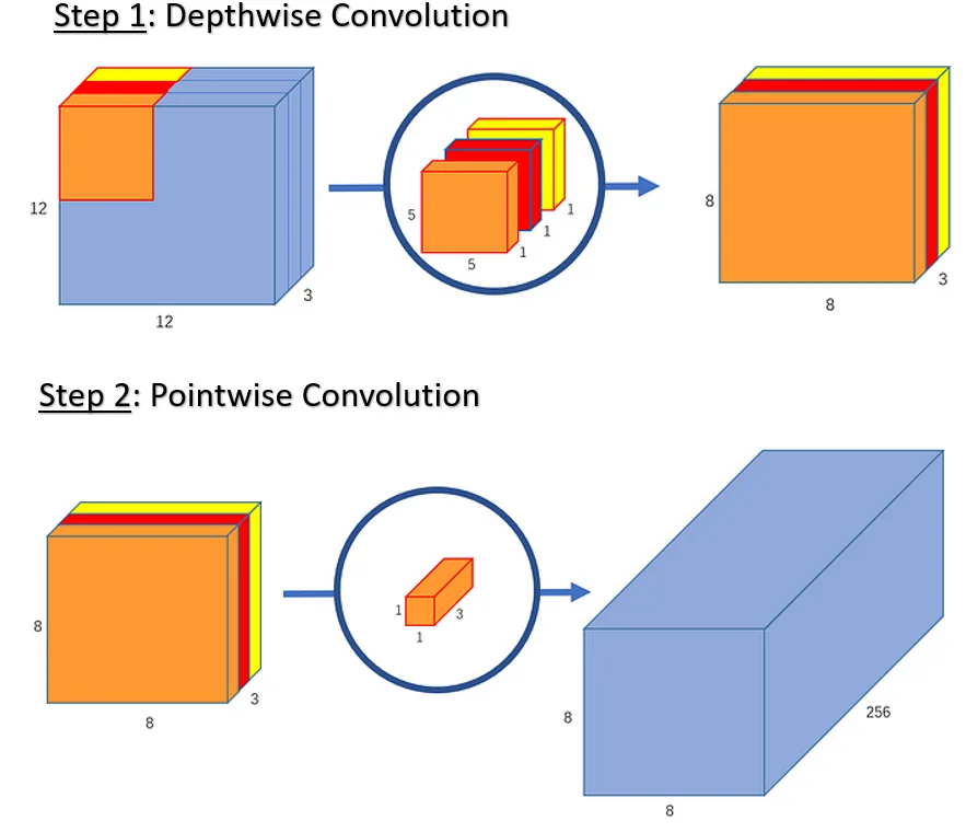
Depthwise separable convolutions separate these roles:
- 1.
- Depthwise (Spatial) Convolution: A \(K \times K\) filter is applied independently to each input channel. For an input feature map of shape \((H \times W \times C_{\mathrm {in}})\), this produces an intermediate feature map of shape \((H \times W \times C_{\mathrm {in}})\). At this stage, each channel learns its own spatial features (e.g., per-channel edge or texture detectors); there is no mixing between channels.
- 2.
- Pointwise (\(1 \times 1\)) Convolution: A bank of \(1 \times 1\) filters then performs a learned linear combination across the \(C_{\mathrm {in}}\) channels at each spatial location. This step mixes information across channels and adjusts the channel dimension from \(C_{\mathrm {in}}\) to \(C_{\mathrm {out}}\), producing an output of shape \((H \times W \times C_{\mathrm {out}})\).
This two-stage “depthwise + pointwise” design is also called channel-wise spatial convolution. Unlike spatially factorized kernels (such as \(3 \times 3\) decomposed into \(1 \times 3\) and \(3 \times 1\)), depthwise separable convolutions do not impose a low-rank constraint on the full kernel, making them easy to insert into existing architectures such as Inception, VGG, or ResNet [106, 239].
Computational and Parameter Efficiency We now compare the computational cost (MACs) and parameter count of a standard \(K \times K\) convolution with its depthwise separable counterpart. For clarity, we consider a single feature map (no batch dimension) of shape \[ (H \times W \times C_{\mathrm {in}}) \quad \longrightarrow \quad (H \times W \times C_{\mathrm {out}}) \] with stride \(1\) and “same” padding, so that the spatial resolution \(H \times W\) stays the same.
Standard \((K \times K)\) Convolution A standard convolution uses \(C_{\mathrm {out}}\) kernels, each of shape \((K \times K \times C_{\mathrm {in}})\). Thus:
- Parameters: \[ \mbox{Params}_{\mbox{std}} = K^2 \, C_{\mathrm {in}} \, C_{\mathrm {out}}. \]
- Multiply-Adds (MACs): There are \(H W C_{\mathrm {out}}\) output elements, each computed as a dot product over \(K^2 C_{\mathrm {in}}\) weights. Therefore: \[ \mbox{MACs}_{\mbox{std}} = (H W C_{\mathrm {out}}) \times (K^2 C_{\mathrm {in}}) = H W K^2 C_{\mathrm {in}} C_{\mathrm {out}}. \]
Depthwise Separable Convolution Depthwise separable convolution decomposes this into:
-
Depthwise Convolution (Spatial Only): We apply one \(K \times K\) filter per input channel, so there are \(C_{\mathrm {in}}\) filters in total. Each filter has shape \((K \times K)\), and each channel is processed independently: \begin {align*} \text {Params}_{\text {depthwise}} &= K^2 \, C_{\mathrm {in}}, \\ \text {MACs}_{\text {depthwise}} &= (H W C_{\mathrm {in}}) \times K^2 = H W K^2 C_{\mathrm {in}}. \end {align*}
The output has shape \((H \times W \times C_{\mathrm {in}})\).
- Pointwise (\(1 \times 1\)) Convolution (Channel Mixing): Next, we apply \(1 \times 1\) filters to mix channels and reach \(C_{\mathrm {out}}\) output channels. Each \(1 \times 1\) kernel has shape \((C_{\mathrm {in}})\), and there are \(C_{\mathrm {out}}\) such kernels: \begin {align*} \text {Params}_{\text {pointwise}} &= C_{\mathrm {in}} \, C_{\mathrm {out}}, \\ \text {MACs}_{\text {pointwise}} &= (H W C_{\mathrm {out}}) \times C_{\mathrm {in}} = H W C_{\mathrm {in}} C_{\mathrm {out}}. \end {align*}
Summing both stages: \begin {align*} \text {Params}_{\text {DSConv}} &= K^2 C_{\mathrm {in}} + C_{\mathrm {in}} C_{\mathrm {out}} = C_{\mathrm {in}} \bigl (K^2 + C_{\mathrm {out}}\bigr ), \\ \text {MACs}_{\text {DSConv}} &= H W K^2 C_{\mathrm {in}} + H W C_{\mathrm {in}} C_{\mathrm {out}} = H W C_{\mathrm {in}} \bigl (K^2 + C_{\mathrm {out}}\bigr ). \end {align*}
Cost Reduction Ratio The reduction in cost when switching from a standard convolution to a depthwise separable convolution is: \[ \frac {\mbox{MACs}_{\mbox{std}}}{\mbox{MACs}_{\mbox{DSConv}}} = \frac {H W K^2 C_{\mathrm {in}} C_{\mathrm {out}}}{H W C_{\mathrm {in}} (K^2 + C_{\mathrm {out}})} = \frac {K^2 C_{\mathrm {out}}}{K^2 + C_{\mathrm {out}}}. \] The same ratio holds for parameter counts. In typical CNNs, \(C_{\mathrm {out}} \gg K^2\) (for example, \(C_{\mathrm {out}} = 256\) and \(K^2 = 9\) for a \(3\times 3\) kernel). In that regime, \[ \frac {K^2 C_{\mathrm {out}}}{K^2 + C_{\mathrm {out}}} \approx K^2, \] so a \(3 \times 3\) depthwise separable convolution is roughly \(9\times \) more efficient than a standard \(3 \times 3\) convolution in both parameters and MACs.
Summary of Costs For convenience, we summarize parameter and MAC counts:
\[ \begin {array}{l|c|c} \textbf {Layer Type} & \textbf {Parameters} & \textbf {MACs} \\ \hline \mbox{Standard } (K \times K) & K^2 C_{\mathrm {in}} C_{\mathrm {out}} & H W K^2 C_{\mathrm {in}} C_{\mathrm {out}} \\[3pt] \mbox{Depthwise} & K^2 C_{\mathrm {in}} & H W K^2 C_{\mathrm {in}} \\[3pt] \mbox{Pointwise } (1 \times 1) & C_{\mathrm {in}} C_{\mathrm {out}} & H W C_{\mathrm {in}} C_{\mathrm {out}} \\[3pt] \mbox{Depthwise Separable (total)} & C_{\mathrm {in}}(K^2 + C_{\mathrm {out}}) & H W C_{\mathrm {in}}(K^2 + C_{\mathrm {out}}) \end {array} \]
Example: \((K=3,\;C_{\mathrm {in}}=128,\;C_{\mathrm {out}}=256,\;H=W=32)\)
Consider an input feature map of shape \((32 \times 32 \times 128)\) and a desired output of shape \((32 \times 32 \times 256)\), using a \(3 \times 3\) kernel, stride \(1\), and “same” padding.
-
Standard Convolution: \begin {align*} \text {Params}_{\text {std}} &= K^2 C_{\mathrm {in}} C_{\mathrm {out}} = 3^2 \cdot 128 \cdot 256 = 294{,}912, \\ \text {MACs}_{\text {std}} &= H W K^2 C_{\mathrm {in}} C_{\mathrm {out}} = 32 \cdot 32 \cdot 9 \cdot 128 \cdot 256 \\ &= 301{,}989{,}888 \approx 3.02 \times 10^8 \text { MACs}. \end {align*}
-
Depthwise Separable Convolution:
- Depthwise step: \begin {align*} \text {Params}_{\text {depthwise}} &= K^2 C_{\mathrm {in}} = 3^2 \cdot 128 = 1{,}152, \\ \text {MACs}_{\text {depthwise}} &= H W K^2 C_{\mathrm {in}} = 32 \cdot 32 \cdot 9 \cdot 128 \\ &= 1{,}179{,}648 \approx 1.18 \times 10^6. \end {align*}
- Pointwise step: \begin {align*} \text {Params}_{\text {pointwise}} &= C_{\mathrm {in}} C_{\mathrm {out}} = 128 \cdot 256 = 32{,}768, \\ \text {MACs}_{\text {pointwise}} &= H W C_{\mathrm {in}} C_{\mathrm {out}} = 32 \cdot 32 \cdot 128 \cdot 256 \\ &= 33{,}554{,}432 \approx 3.36 \times 10^7. \end {align*}
Total depthwise separable cost: \begin {align*} \text {Params}_{\text {DSConv}} &= 1{,}152 + 32{,}768 = 33{,}920, \\ \text {MACs}_{\text {DSConv}} &= 1{,}179{,}648 + 33{,}554{,}432 = 34{,}734{,}080 \approx 3.47 \times 10^7. \end {align*}
Comparing the two: \[ \frac {\mbox{Params}_{\mbox{std}}}{\mbox{Params}_{\mbox{DSConv}}} = \frac {294{,}912}{33{,}920} \approx 8.69, \qquad \frac {\mbox{MACs}_{\mbox{std}}}{\mbox{MACs}_{\mbox{DSConv}}} = \frac {301{,}989{,}888}{34{,}734{,}080} \approx 8.69. \] Thus, in this realistic setting, replacing a standard \(3 \times 3\) convolution with a depthwise separable convolution reduces both parameters and computation by almost an order of magnitude, while still allowing the network to first learn rich spatial filters per channel and then flexibly mix them across channels in the pointwise step.
Reduction Factor By separating spatial and channel mixing, depthwise separable convolutions can reduce computational cost by up to an order of magnitude in many practical scenarios, enabling advanced CNNs to run on mobile or embedded devices with minimal resource usage.
A common approximate reduction ratio is: \[ \frac {\mbox{Cost}_\mbox{DSConv}}{\mbox{Cost}_\mbox{StdConv}} \;\approx \; \frac {C_{\mbox{in}} \times K^2 + C_{\mbox{in}} \times C_{\mbox{out}}}{C_{\mbox{in}} \times C_{\mbox{out}} \times K^2} \;=\; \frac {1}{C_{\mbox{out}}} + \frac {1}{K^2}. \] As an example, for \(K=3\) and \(C_{\mbox{out}}=256\), the ratio is \(\frac {1}{256} + \frac {1}{9} \approx 0.11\), i.e. about a \(\sim 9\times \) reduction in FLOPs compared to a standard \(3\times 3\) convolution.
- MobileNet [239]: Relies on depthwise separable layers to achieve low-latency inference on mobile devices.
- ShuffleNet [801]: Combines depthwise separable convs with a channel shuffle operation to further improve efficiency.
- Xception [106]: Extends Inception-like modules by fully replacing standard convolutions with depthwise separable variants for all spatial operations.
- EfficientNet [621]: Integrates depthwise separable layers in a compound scaling framework, balancing network width, depth, and resolution.
- Reduced Cross-Channel Expressiveness: A standard convolution captures both spatial patterns and cross-channel correlations in a single operation: each \(K \times K\) filter integrates information from all \(C_{\mathrm {in}}\) channels over its receptive field before the nonlinearity, enabling rich, intertwined feature interactions. Depthwise separable convolutions factorize this process. The depthwise stage applies spatial filters independently to each channel (no inter-channel mixing), and the subsequent pointwise \(1 \times 1\) stage performs only linear combinations across channels at fixed spatial positions. Although stacking several depthwise separable blocks still allows complex dependencies to emerge (pointwise mixing in one block feeds into depthwise spatial filtering in the next), this sequential mechanism is less expressive per layer than a monolithic standard convolution. Interactions that one standard layer can model directly may require multiple depthwise separable layers to approximate, potentially making optimization harder and slightly reducing representational power. To compensate, modern architectures often incorporate explicit cross-channel modeling modules such as Squeeze-and-Excitation (SE) blocks or attention mechanisms, which adaptively reweight channels and restore some of the lost flexibility [244, 106].
- Substantial Compute Savings: By decoupling spatial filtering \(\bigl (O(K^2 C_{\mathrm {in}})\bigr )\) from channel mixing \(\bigl (O(C_{\mathrm {in}} C_{\mathrm {out}})\bigr )\), depthwise separable convolutions reduce MACs and parameters by factors of roughly \(K^2\) for typical settings (e.g., \(\sim 8\mbox{--}9\times \) for \(K=3\), large \(C_{\mathrm {out}}\)), as shown in the previous cost analysis. This dramatic efficiency gain is crucial for real-time inference on resource-constrained devices such as smartphones, embedded boards, or edge accelerators, often with only a modest drop in accuracy.
Overall, depthwise separable convolutions have become a cornerstone of efficient CNN design, trading a small amount of per-layer expressiveness for large reductions in computation and parameter count, and thereby enabling high-performing models in mobile and embedded environments.
7.8.7 Summary of Specialized Convolutions
- 1x1 convolutions: Used for feature selection, dimensionality reduction, and efficient computation.
- 1D convolutions: Applied in sequential data processing, such as text and audio.
- 3D convolutions: Extend feature extraction to volumetric and spatiotemporal data.
- Spatial separable convolutions: Factorize standard convolutions into separate width and height operations, reducing computation while maintaining output dimensions. Unfortunately, these convolutions are not common as only special filters can be spatially separated, which makes this type of convolutions impractical for deep learning purposes.
- Depthwise separable convolutions: Split convolutions into depthwise and pointwise operations, significantly reducing computational cost while preserving some feature extraction capabilities, making it useful in efficient/mobile architectures where speed is a critical factor.
These specialized convolutions enhance the flexibility and efficiency of neural networks, enabling them to process diverse types of structured data, over different computation platforms (from expensive and powerful GPU servers up to common mobile devices).
7.11 Pooling Layers
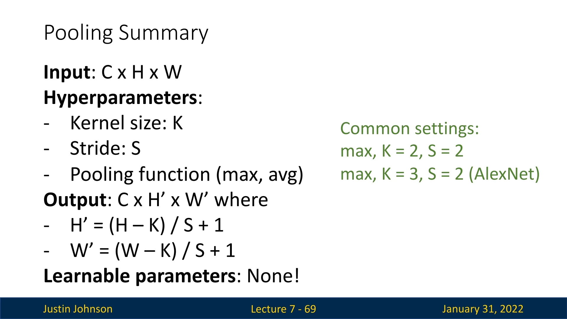
Pooling layers are a key component of convolutional neural networks (CNNs), serving to condense spatial information and highlight the most salient features of an input. Unlike convolutional layers, which learn filters, pooling layers have no learnable parameters; they instead apply a fixed aggregation function (such as maximum or average) over local neighborhoods. Hyperparameters such as the kernel size, stride, and pooling type control the degree of downsampling. This simple yet powerful mechanism reduces feature map resolution, lowers computational cost, increases robustness to spatial variations, and expands the effective receptive field in deeper layers.
7.9.1 Types of Pooling
Pooling operates much like a convolution: a window slides across the feature map according to the stride, and a function is applied within each region to produce one representative value. When the stride equals the kernel size, the pooling regions are non-overlapping.
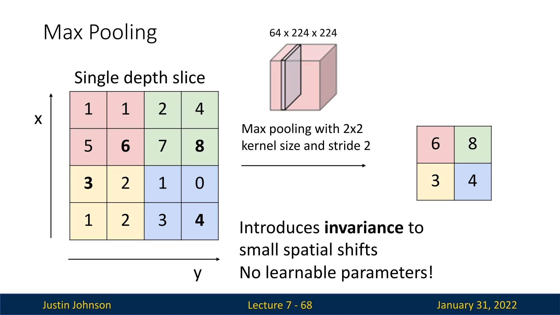
- Max Pooling: Selects the maximum activation within each window, retaining the strongest response and emphasizing dominant local features.
- Average Pooling: Computes the average value within each window, creating a smoother, more generalized representation of the feature map. However, excessive averaging can blur fine details or weaken distinctive local patterns.
7.9.2 Effect and Benefits of Pooling
Pooling summarizes local activations to form a more compact and abstract feature representation. By keeping only the strongest or average responses in each region, the network becomes more efficient and more robust. The main benefits include:
- Reduced Computation and Memory: Pooling decreases the spatial resolution of feature maps, lowering the number of activations passed to deeper layers. This directly reduces both computational load and memory requirements.
- Translation Invariance: Pooling introduces robustness to small translations or distortions in the input. A feature that shifts slightly within its receptive field is still captured after pooling, making the network less sensitive to exact spatial alignment.
- Improved Generalization: By discarding minor local variations, pooling acts as a form of regularization, reducing the risk of overfitting to fine-grained details or noise present in the training data.
- Expanded Receptive Field: Since pooling reduces the resolution of intermediate representations, subsequent convolutional layers operate over proportionally larger portions of the original input. This allows deeper layers to integrate global spatial context and capture more abstract patterns.
In summary, pooling layers help CNNs focus on the most informative spatial cues while controlling computational complexity and promoting invariance—key ingredients for robust hierarchical feature learning.
Enrichment 7.11.3: Pooling Layers in Backpropagation
Pooling layers are commonly used in convolutional neural networks (CNNs) to reduce spatial dimensions while retaining important features. The two most common types are max pooling and average pooling. Understanding how backpropagation works for these layers is important, since it determines how error signals are routed back to earlier feature maps.
Forward Pass of Pooling Layers
Pooling operates on small regions (e.g., a \(2 \times 2\) window) and reduces each region to a single value, downsampling the feature map without introducing learnable parameters:
- Max pooling: Selects the maximum value from the window, emphasizing dominant activations.
- Average pooling: Computes the average of all values in the window, yielding a smoothed summary.
Example of Forward Pass Consider a single \(4 \times 4\) input matrix \(X\); we will use the same \(X\) for both the forward and backward pass examples:
\[ X = \begin {bmatrix} 1 & 3 & 2 & 1 \\ \mathbf {4} & 2 & 1 & \mathbf {5} \\ 2 & 0 & \mathbf {3} & 1 \\ 1 & \mathbf {5} & 2 & 2 \end {bmatrix} \]
We apply a \(2 \times 2\) pooling window with stride 2, giving four non-overlapping regions (quadrants).
Max pooling computes: \[ Y_{\mbox{max}} = \begin {bmatrix} \max (1,3,\mathbf {4},2) & \max (2,1,1,\mathbf {5}) \\[4pt] \max (2,0,1,\mathbf {5}) & \max (\mathbf {3},1,2,2) \end {bmatrix} = \begin {bmatrix} 4 & 5 \\ 5 & 3 \end {bmatrix}. \] The max positions in \(X\) are: \[ (1,0),\ (1,3),\ (3,1),\ (2,2). \]
Average pooling computes: \[ Y_{\mbox{avg}} = \begin {bmatrix} \frac {1+3+4+2}{4} & \frac {2+1+1+5}{4} \\[4pt] \frac {2+0+1+5}{4} & \frac {3+1+2+2}{4} \end {bmatrix} = \begin {bmatrix} 2.5 & 2.25 \\ 2 & 2 \end {bmatrix}. \]
Backpropagation Through Pooling Layers
During backpropagation, we propagate gradients from the pooled outputs back to the inputs. Let the upstream gradient with respect to the pooled output be \[ \frac {\partial L}{\partial Y} = \begin {bmatrix} 0.2 & -0.3 \\ 0.4 & 0.1 \end {bmatrix}, \] where \(L\) is the loss. We now see how this gradient is mapped back to \(\frac {\partial L}{\partial X}\).
Max Pooling Backpropagation For max pooling, the gradient from each pooled value is passed back only to the input element that was the maximum in that window; all other elements in the window receive zero gradient. This makes max pooling behave like a “routing” operation for gradients.
Using the max locations from the forward pass:
- The gradient \(0.2\) (from the top-left pooled output) is assigned to \(X_{1,0}\).
- The gradient \(-0.3\) (top-right) is assigned to \(X_{1,3}\).
- The gradient \(0.4\) (bottom-left) is assigned to \(X_{3,1}\).
- The gradient \(0.1\) (bottom-right) is assigned to \(X_{2,2}\).
Thus the downstream gradient with respect to \(X\) is: \[ \frac {\partial L}{\partial X} = \begin {bmatrix} 0 & 0 & 0 & 0 \\ \mathbf {0.2} & 0 & 0 & \mathbf {-0.3} \\ 0 & 0 & \mathbf {0.1} & 0 \\ 0 & \mathbf {0.4} & 0 & 0 \end {bmatrix}. \]
- Sparse gradients: Only the max positions in each window receive nonzero gradients, while all other activations are ignored in backpropagation. This sparsity can slow learning, since fewer units contribute to the parameter updates.
- Reduced feedback to fine details: Because non-max activations receive no gradient, small but potentially informative responses may not be reinforced, which can matter in tasks that require precise spatial detail.
To alleviate excessive sparsity, modern architectures sometimes use overlapping pooling (stride smaller than window size) or replace pooling entirely with strided convolutions, which maintain dense gradient flow through learnable filters.
Average Pooling Backpropagation For average pooling, the gradient from each pooled output is distributed evenly among all elements in its window. If a window contains \(n\) elements, each input in that window receives \(\frac {1}{n}\) of the upstream gradient.
In our example, each \(2 \times 2\) window has \(n=4\) elements, so we divide each entry of \(\frac {\partial L}{\partial Y}\) by 4:
- Top-left window: \(0.2 / 4 = 0.05\).
- Top-right window: \(-0.3 / 4 = -0.075\).
- Bottom-left window: \(0.4 / 4 = 0.1\).
- Bottom-right window: \(0.1 / 4 = 0.025\).
The resulting gradient with respect to \(X\) is dense: \[ \frac {\partial L}{\partial X} = \begin {bmatrix} 0.05 & 0.05 & -0.075 & -0.075 \\ 0.05 & 0.05 & -0.075 & -0.075 \\ 0.1 & 0.1 & 0.025 & 0.025 \\ 0.1 & 0.1 & 0.025 & 0.025 \end {bmatrix}. \]
General Backpropagation Rules for Pooling
For a pooling window with inputs \(\{x_i\}_{i=1}^n\), pooled output \(O\), and upstream gradient \(\frac {\partial L}{\partial O}\), the local gradients are:
- Max pooling: Let \(x_{\max }\) be the input that attained the maximum in the forward pass. Then \[ \frac {\partial L}{\partial x_i} = \begin {cases} \frac {\partial L}{\partial O} & \mbox{if } x_i = x_{\max }, \\ 0 & \mbox{otherwise}. \end {cases} \]
- Average pooling: All inputs share the gradient equally: \[ \frac {\partial L}{\partial x_i} = \frac {1}{n}\,\frac {\partial L}{\partial O} \quad \mbox{for all } i = 1,\dots ,n. \]
These rules emphasize the conceptual difference between max and average pooling in backpropagation: max pooling routes gradients through a few dominant activations, whereas average pooling spreads gradients more uniformly across all inputs in each region.
7.9.3 Global Pooling Layers
Global pooling layers apply a pooling operation over the entire spatial dimension of a feature map, unlike regular pooling (e.g., \(2\times 2\)) which operates on smaller local regions. By collapsing each feature map into a single value, these layers often replace fully connected (FC) layers at the end of convolutional networks, drastically reducing parameter counts.
General Advantages
- More Robustness to Overfitting: Global pooling removes the need for large FC layers. It doesn’t introduce additional learnable weights, and merely aggregates existing activations. Hence, using it significantly cuts the number of trainable parameters.
- Lightweight Alternative to FC Layers: Rather than flattening high-dimensional feature maps, introducing several MLP layers at the end of the CNN, a single value per map suffices, increasing computation speed while decreasing the size of the model.
- Improved Generalization: Summarizing or selecting the strongest feature responses promotes focusing on essential aspects of the learned representation.
Global Average Pooling (GAP)
Operation GAP computes the mean of all activations in a feature map \(X\in \mathbb {R}^{H\times W}\): \[ O = \frac {1}{HW}\sum _{i=1}^{H}\sum _{j=1}^{W} X_{ij}. \] This is performed independently for each channel.
- Direct Channel-to-Feature Mapping: Each channel in the input shrinks to a single numeric representation, facilitating interpretability.
- Smooth Gradient Flow: Since every spatial element contributes equally, gradients are spread out evenly, stabilizing training.
- Loss of Spatial Detail: Global averaging discards where a feature occurs.
- Sensitivity to Very Small Feature Maps: If \((H,W)\) is tiny, the mean could be too coarse, omitting relevant details.
Backpropagation Since \(O\) is the average over \(HW\) elements, \[ \frac {\partial L}{\partial X_{ij}} = \frac {\partial L}{\partial O}\times \frac {1}{HW}. \]
Global Max Pooling (GMP)
Operation. GMP takes the maximum over \(\{X_{ij}\}\) in a feature map: \[ O = \max _{i,j} X_{ij}. \]
- Captures Strongest Activations: Highlights the most prominent response within the map.
- Useful in Detection Tasks: Identifying a key active neuron can help in bounding box predictions or coarse localization.
- Sparse Gradient Updates: Only the max element receives gradient signals; others get zero, potentially harming learning.
- Overemphasis on a Single Activation: Non-max elements, which might contain relevant sub-features, are ignored.
Backpropagation Only the maximum entry obtains a nonzero derivative: \[ \frac {\partial L}{\partial X_{ij}} = \begin {cases} \frac {\partial L}{\partial O}, & \mbox{if } X_{ij}=O,\\ 0, & \mbox{otherwise}. \end {cases} \]
Comparison of GAP and GMP
| Layer | Computation | Gradient Flow |
|---|---|---|
| Global Average Pooling | Mean of all elements | Evenly distributed |
| Global Max Pooling | Single maximum element | Only max location receives updates |
Contrasting with Regular Pooling
- Regular Pooling: Uses smaller windows (\(2\times 2\), \(3\times 3\), …) gradually reducing dimensions, preserving some notion of spatial layout.
- Global Pooling: Collapses the entire feature map to one value per channel, often as a final layer (or near the end).
- To replace fully connected layers, common in many efficient CNN architectures like MobileNet.
- When a concise channel-level summary suffices (e.g. final classification).
- Early or mid-layer dimension reduction where preserving partial spatial context is beneficial.
- Tasks requiring finer feature localization (e.g. segmentation).
7.12 Classical CNN Architectures
Now that we have covered fully connected layers, activation functions, convolutional layers, and pooling layers, we can begin exploring classical Convolutional Neural Network (CNN) architectures. One of the earliest and most influential architectures is LeNet-5, developed by Yann LeCun in 1998 for handwritten character recognition [326]. This model laid the foundation for modern CNNs, demonstrating how multiple convolutional and pooling layers can be stacked to learn hierarchical representations.
7.10.1 LeNet-5 Architecture
LeNet-5 follows the classical approach of multiple blocks of \([ \mbox{Conv}, \mbox{ReLU}, \mbox{Pool} ]\), meaning: \[ \left [ \mbox{Conv}, \mbox{ReLU}, \mbox{Pool} \right ] \times N \] where \(N\) denotes the number of convolutional blocks. After progressively reducing the spatial dimensionality while increasing the number of feature channels, the architecture flattens the output and applies additional fully connected layers: \[ \left [ \mbox{FC}, \mbox{ReLU} \right ] \times M, \mbox{ followed by an FC output layer.} \] The final layer typically performs classification using Softmax or another activation function suited to the task.
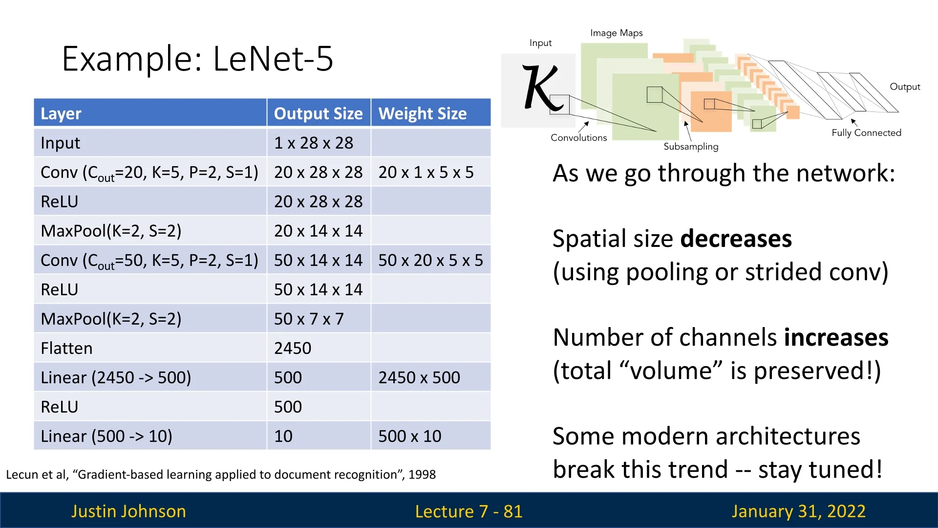
Detailed Layer Breakdown
- Input: A grayscale \(28 \times 28\) image, represented as a tensor of shape \(1 \times 28 \times 28\) (one channel, height 28, width 28). This example assumes processing one image at a time rather than a batch.
-
First Convolutional Layer:
- Number of output channels: \(C_{\mbox{out}} = 20\).
- Kernel size: \(K = 5\), padding: \(P = 2\), stride: \(S = 1\).
- Output spatial size remains \(28 \times 28\) due to same padding, but now with 20 channels.
- Output tensor shape: \(20 \times 28 \times 28\).
- Filter weight dimensions: \(20 \times 1 \times 5 \times 5\).
- Activation: ReLU applied, preserving the output shape.
-
First Pooling Layer:
- Type: Max Pooling.
- Kernel size: \(K = 2\), stride: \(S = 2\).
- Reduces spatial dimensions to \(14 \times 14\) while keeping 20 channels.
- Output tensor shape: \(20 \times 14 \times 14\).
- No additional learnable parameters.
-
Second Convolutional Layer:
- Number of output channels: \(C_{\mbox{out}} = 50\).
- Kernel size: \(K = 5\), padding: \(P = 2\), stride: \(S = 1\).
- Output spatial size remains \(14 \times 14\) (same padding).
- Output tensor shape: \(50 \times 14 \times 14\).
- Filter weight dimensions: \(50 \times 20 \times 5 \times 5\).
- Activation: ReLU applied.
-
Second Pooling Layer:
- Type: Max Pooling.
- Kernel size: \(K = 2\), stride: \(S = 2\).
- Reduces spatial dimensions to \(7 \times 7\), maintaining 50 channels.
- Output tensor shape: \(50 \times 7 \times 7\).
- No additional learnable parameters.
-
Flattening Layer:
- Converts \(50 \times 7 \times 7\) into a single vector of \(2450\) elements.
-
Fully Connected Layers:
-
First FC layer:
- Output size: 500 neurons.
- Weights: \(2450 \times 500\).
- Activation: ReLU.
-
Second FC layer (output layer):
- Output size: 10 neurons (assuming classification into 10 classes).
- Weights: \(500 \times 10\).
- Activation: Softmax (for classification tasks).
-
Summary of LeNet-5
| Layer | Output Shape | Filter Size | Parameters |
|---|---|---|---|
| Input | \(1 \times 28 \times 28\) | - | 0 |
| Conv1 | \(20 \times 28 \times 28\) | \(5 \times 5\) | \(20 \times 1 \times 5 \times 5\) |
| Pool1 | \(20 \times 14 \times 14\) | \(2 \times 2\) | 0 |
| Conv2 | \(50 \times 14 \times 14\) | \(5 \times 5\) | \(50 \times 20 \times 5 \times 5\) |
| Pool2 | \(50 \times 7 \times 7\) | \(2 \times 2\) | 0 |
| Flatten | \(2450\) | - | 0 |
| FC1 | \(500\) | - | \(2450 \times 500\) |
| FC2 | \(10\) | - | \(500 \times 10\) |
Key Architectural Trends in CNNs, Illustrated by LeNet-5
Hierarchical Feature Learning LeNet-5 demonstrated how progressively reducing spatial dimensions while increasing channel depth leads to feature representations that capture multiple abstraction levels (edges, textures, shapes, etc.).
Alternating Convolution and Pooling By interleaving convolutional and pooling layers, the network efficiently extracts features while gradually shrinking the spatial resolution, reducing both compute and parameter counts.
Transition to Fully Connected (FC) Layers After sufficient feature extraction in convolutional/pooling blocks, LeNet-5 relies on FC layers to finalize classification or regression tasks—an approach still prevalent in many CNNs.
7.10.2 How Are CNN Architectures Designed?
Designing a modern CNN involves balancing multiple factors:
- Spatial Reduction vs. Feature Expansion: Typical CNNs downsample \((H \times W)\) over depth while increasing the number of channels. This balance preserves rich representational capacity without bloating the parameter count.
- Depth and Network Complexity: Deeper networks can model more complex structures but face potential pitfalls like vanishing or exploding gradients. Architectures increasingly include smarter activation function choices (e.g., replacing Sigmoid with ReLU based activations), batch normalization layers, and skip connections (to be covered later) to mitigate these issues in training deep CNNs.
- Computational Efficiency: Streamlined designs avoid excessive parameters to ensure faster training and real-time inference, especially crucial in mobile or embedded contexts.
Enrichment 7.13: Vanishing & Exploding Gradients: A Barrier to DL
Context As deep learning evolved, researchers encountered fundamental challenges in training deep neural networks (DNNs), particularly the vanishing and exploding gradient problems. These issues severely limited the depth of trainable models, preventing effective learning in deep architectures. It wasn’t until methods like Batch Normalization (BN) and Residual Connections emerged that training very deep networks became feasible.
Throughout the next chapters of this summary, we’ll address these modern solutions and others. Nevertheless, it’s important to begin by defining and analyzing these gradient-related challenges, which is the goal of this enrichment.
Enrichment 7.13.1: Understanding the Problem
The Role of Gradients in Deep Networks
Training deep neural networks relies on backpropagation, where gradients propagate backward through the network to update weights. However, in deep architectures, this process often suffers from two critical issues:
- Vanishing Gradients: If gradients shrink exponentially, earlier layers receive near-zero updates, making learning inefficient.
- Exploding Gradients: If gradients grow exponentially, updates become excessively large, leading to instability and divergence.
Gradient Computation in Deep Networks
Backpropagation updates network parameters by computing gradients recursively using the chain rule. For a weight \( w^{(i)} \) in layer \( i \), the gradient of the loss function \( \mathcal {L} \) with respect to \( w^{(i)} \) is given by:
\begin {equation} \begin {aligned} \frac {\partial \mathcal {L}}{\partial w^{(i)}} &= \frac {\partial \mathcal {L}}{\partial a^{(L)}} \frac {\partial a^{(L)}}{\partial z^{(L)}} \frac {\partial z^{(L)}}{\partial a^{(L-1)}} \cdots \frac {\partial z^{(i+1)}}{\partial a^{(i)}} \frac {\partial a^{(i)}}{\partial z^{(i)}} \frac {\partial z^{(i)}}{\partial w^{(i)}} \\ &\underbrace {=}_{\mbox{Multiplication Commutativity}} \frac {\partial \mathcal {L}}{\partial a^{(L)}} \underbrace {\prod _{j=i+1}^{L} \frac {\partial z^{(j)}}{\partial a^{(j-1)}}}_{\mbox{Accumulated Weight Multiplication}} \cdot \frac {\partial z^{(i)}}{\partial w^{(i)}} \cdot \underbrace {\prod _{j=i}^{L} \frac {\partial a^{(j)}}{\partial z^{(j)}}}_{\mbox{Accumulated Activation Derivatives}} \end {aligned} \label {eq:gradient_general} \end {equation}
This equation explicitly shows how gradients propagate through the network and accumulate a product of derivatives.
Key Components of Gradient Propagation Each term in the equation plays a crucial role in determining how gradients behave during backpropagation:
- \( z^{(j)} \) represents the pre-activation output at layer \( j \), computed as the weighted sum of activations from the previous layer: \[ z^{(j)} = W^{(j)} a^{(j-1)} \] where \( W^{(j)} \) is the weight matrix and \( a^{(j-1)} \) is the activation from the previous layer.
- \( a^{(j)} \) represents the activation output at layer \( j \), obtained by applying the activation function \( \phi \) to \( z^{(j)} \): \[ a^{(j)} = \phi (z^{(j)}) \]
- The term \( \frac {\partial a^{(j)}}{\partial z^{(j)}} \) is the derivative of the activation function, which directly influences whether gradients vanish or explode. This term appears as: \[ \underbrace {\prod _{j=i}^{L} \frac {\partial a^{(j)}}{\partial z^{(j)}}}_{\mbox{Activation Gradients Accumulation}} \] If most activation derivatives satisfy \( \left | \frac {\partial a^{(j)}}{\partial z^{(j)}} \right | < 1 \), their repeated multiplication can result in an exponentially small value, leading to vanishing gradients. Not only that, if one of the derivatives turns out to be 0, the entire gradient gets nullified. Conversely, if \( \left | \frac {\partial a^{(j)}}{\partial z^{(j)}} \right | > 1 \), their product rapidly grows, potentially causing exploding gradients.
- The term \( \frac {\partial z^{(j)}}{\partial a^{(j-1)}} \) represents the weight multiplication before applying activation: \[ \frac {\partial z^{(j)}}{\partial a^{(j-1)}} = W^{(j)} \] This term accumulates as: \[ \underbrace {\prod _{j=i+1}^{L} \frac {\partial z^{(j)}}{\partial a^{(j-1)}}}_{\mbox{Weight Matrices Accumulation}} \] If the weight matrices \( W^{(j)} \) have large values, their product amplifies the gradient magnitude, potentially leading to exploding gradients. If they are too small, the gradient shrinks, exacerbating vanishing gradients. Not only that, if one of the weight matrices turns out to be 0, the entire gradient gets nullified as well.
Impact of Depth in Neural Networks
Deep neural networks (DNNs) contain many layers, making them powerful feature extractors but also susceptible to gradient instability. During backpropagation, the gradient of the loss function with respect to early-layer parameters is computed as a product of many local derivatives. Specifically, for a weight \( w^{(1)} \) in the first layer, we observe:
\[ \frac {\partial \mathcal {L}}{\partial w^{(1)}} \propto \prod _{j=1}^{L} \frac {\partial a^{(j)}}{\partial z^{(j)}}, \]
where \( \frac {\partial a^{(j)}}{\partial z^{(j)}} \) represents the local activation derivative at each layer. Since modern deep networks are built with large \( L \), this product accumulates a large number of terms, amplifying either vanishing or exploding gradients.
-
Vanishing Gradients: If most activation derivatives satisfy \[ \left |\frac {\partial a^{(j)}}{\partial z^{(j)}}\right | < 1, \] then their repeated multiplication causes the gradient to shrink exponentially: \[ \prod _{j=1}^{L} \frac {\partial a^{(j)}}{\partial z^{(j)}} \approx \left ( \frac {\partial a}{\partial z} \right )^{L}. \] As \( L \) grows larger, this product approaches zero, preventing effective weight updates in earlier layers. Consequently, these layers fail to learn meaningful representations, leading to slow or stalled training. A similar effect occurs when weight matrices contain very small values, further diminishing the gradient:
\[ \prod _{j=2}^{L} W^{(j)} \approx \left (W\right )^{L}. \]
If most \( W^{(j)} \) values are small (\( |W| < 1 \)), then the gradient rapidly decreases across layers, compounding the vanishing gradient problem.
-
Exploding Gradients: Conversely, if most activation derivatives satisfy \[ \left |\frac {\partial a^{(j)}}{\partial z^{(j)}}\right | > 1, \] their product grows exponentially: \[ \prod _{j=1}^{L} \frac {\partial a^{(j)}}{\partial z^{(j)}} \approx \left ( \frac {\partial a}{\partial z} \right )^{L}. \] As \( L \) increases, this product grows indefinitely, leading to excessively large gradients that destabilize training. Similarly, if most weight matrices have large values (\( |W| > 1 \)), then their product amplifies gradients:
\[ \prod _{j=2}^{L} W^{(j)} \approx \left (W\right )^{L}. \]
In this case, updates become erratic, causing weight oscillations and divergence during training.
Thus, both the choice of activation functions (which determine local derivatives) and the scale of weight matrices are crucial in maintaining a stable gradient flow. A proper balance prevents gradients from vanishing or exploding, ensuring effective training in deep networks.
Practical Example: Vanishing Gradients with Sigmoid Activation
To illustrate the vanishing gradient problem, consider a deep neural network with \( L = 10 \) layers, where each layer uses the sigmoid activation function:
\[ \sigma (z) = \frac {1}{1+e^{-z}} \]
The derivative of the sigmoid function is:
\[ \sigma '(z) = \sigma (z) (1 - \sigma (z)) \]
Since \( \sigma (z) \) outputs values in the range \( (0,1) \), its derivative satisfies:
\[ 0 < \sigma '(z) \leq 0.25, \quad \mbox{with maximum at } \sigma (0) = 0.5. \]
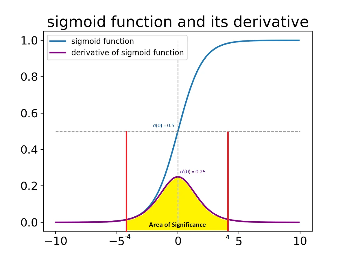
Using this activation function, we analyze the gradient of the loss function \( \mathcal {L} \) with respect to the weight \( w^{(1)} \) in the first layer:
\begin {equation} \begin {aligned} \frac {\partial \mathcal {L}}{\partial w^{(1)}} &= \frac {\partial \mathcal {L}}{\partial a^{(L)}} \underbrace {\prod _{j=2}^{L} \frac {\partial z^{(j)}}{\partial a^{(j-1)}}}_{\mbox{Weight Multiplications}} \cdot \frac {\partial z^{(1)}}{\partial w^{(1)}} \cdot \underbrace {\prod _{j=1}^{L} \frac {\partial a^{(j)}}{\partial z^{(j)}}}_{\mbox{Activation Gradients}}. \end {aligned} \label {eq:gradient_first_layer_example} \end {equation}
Effect of Activation Gradients
Focusing on the activation gradient term:
\[ \prod _{j=1}^{L} \frac {\partial a^{(j)}}{\partial z^{(j)}} \]
Since we assumed a sigmoid activation where each derivative satisfies \( \frac {\partial a^{(j)}}{\partial z^{(j)}} \leq 0.25 \), this product behaves as:
\[ \prod _{j=1}^{10} \frac {\partial a^{(j)}}{\partial z^{(j)}} \leq 0.25^{10}. \]
Computing this numerically:
\[ 0.25^{10} = \left ( \frac {1}{4} \right )^{10} = \frac {1}{1048576} \approx 9.5 \times 10^{-7}. \]
This shows that the gradient contribution from activation derivatives shrinks exponentially, leading to near-zero updates for the first layer.
Effect of Weight Multiplications
Now, consider the weight multiplication term:
\[ \prod _{j=2}^{L} \frac {\partial z^{(j)}}{\partial a^{(j-1)}} = \prod _{j=2}^{10} W^{(j)}. \]
The weight matrices \( W^{(j)} \) determine how activations are transformed before passing through activation functions. If these weights are small (e.g., \( |W^{(j)}| < 1 \)), their product further reduces the gradient magnitude.
For instance, assuming \( |W^{(j)}| = 0.3 \):
\[ \prod _{j=2}^{10} W^{(j)} \approx (0.3)^{9} = 1.97 \times 10^{-5}. \]
This demonstrates that even with moderate weight magnitudes, the accumulated product significantly reduces the gradient. When coupled with the vanishing gradients caused by activation functions like the sigmoid, this effect becomes even more pronounced.
Conclusion: Vanishing Gradients
The total gradient for the first layer’s weights is:
\[ \frac {\partial \mathcal {L}}{\partial w^{(1)}} \approx (9.5 \times 10^{-7}) \times (1.97 \times 10^{-5}) \times \frac {\partial \mathcal {L}}{\partial a^{(L)}} \]
which results in an extremely small value. This means that early layers receive negligible updates, making it difficult for the network to learn meaningful features in deeper architectures.
This example highlights why deep networks struggle to train without techniques such as:
- Batch Normalization, which rescales activations to maintain stable gradients by normalizing feature distributions across mini-batches. This helps prevent activations from becoming too large or too small, stabilizing training and improving gradient propagation.
- Careful Weight Initialization, ensuring that weight magnitudes are neither too small nor too large. Proper initialization strategies, such as Xavier or He initialization, help maintain stable variance of activations across layers, reducing the risk of vanishing or exploding gradients.
- Alternative Activation Functions, such as ReLU, which mitigates vanishing gradients by maintaining nonzero derivatives for positive inputs. Unlike the sigmoid function, which saturates for large positive or negative inputs and produces near-zero gradients, ReLU retains a derivative of 1 for all positive values. This allows gradients to flow more effectively through the network. However, ReLU can suffer from the dying ReLU problem, where neurons output zero and stop updating. Variants such as Leaky ReLU and ELU address this by allowing small negative gradients for negative inputs.
- Residual Connections, which introduce identity mappings to allow gradient flow across layers, effectively mitigating vanishing gradients in very deep networks. In standard deep architectures, gradients can become exponentially small as they propagate backward. Residual connections, used in architectures like ResNet, create shortcut pathways that allow gradients to bypass multiple layers. This ensures that earlier layers receive meaningful updates, making it possible to train networks with hundreds of layers.
Each of these techniques plays a crucial role in modern deep learning architectures, and we will thoroughly investigate them in later sections of this document. Understanding their impact is essential for designing networks that can scale effectively without suffering from unstable gradient behavior.
7.14 Batch Normalization
Training deep neural networks presents several challenges, such as unstable gradients and slow convergence. Normalization layers address these issues by stabilizing and accelerating training. The most widely used normalization layer is Batch Normalization (BatchNorm), introduced by Ioffe and Szegedy in 2015 [265]. The core idea behind BatchNorm is to normalize the activations of each layer to have zero mean and unit variance, ensuring more stable distributions during training.
7.11.1 Understanding Mean, Variance, and Normalization
Before introducing the Batch Normalization process, it is essential to understand the statistical concepts of mean, variance, and normalization. These concepts help explain why BatchNorm improves neural network training.
Mean: The mean (or average) of a set of values provides a central reference point and is computed as:
\begin {equation} \mu _i = \frac {1}{N} \sum _{j=1}^{N} x_i^{(j)} \end {equation}
where is the number of observations in the dataset (or batch), and represents each sample in the feature dimension . The mean provides an estimate of the central tendency of the dataset.
Variance: The variance quantifies the spread of values around the mean and is given by:
\begin {equation} \sigma _i^2 = \frac {1}{N} \sum _{j=1}^{N} (x_i^{(j)} - \mu _i)^2 \end {equation}
Variance measures how much the values deviate from the mean. A high variance indicates that values are spread out, while a low variance suggests they are clustered closely around the mean.
Standard Deviation: The standard deviation is simply the square root of the variance:
\begin {equation} \sigma _i = \sqrt {\sigma _i^2} = \sqrt {\frac {1}{N} \sum _{j=1}^{N} (x_i^{(j)} - \mu _i)^2} \end {equation}
It provides an interpretable measure of dispersion, showing how much values deviate from the mean in the same unit as the original data.
Effect of Normalization: When normalizing values to have zero mean and unit variance, we apply the transformation:
\begin {equation} \hat {x}_i = \frac {x_i - \mu _i}{\sigma _i} \end {equation}
This process ensures that each feature has a consistent scale, preventing some features from dominating the learning process.
7.11.2 Internal Covariate Shift and Batch Normalization’s Role
The authors of the BatchNorm paper proposed that their layer helps mitigate a non-rigorous phenomenon known as Internal Covariate Shift, which can slow down training and reduce model robustness.
What is Covariate Shift? Covariate shift occurs when the distribution of features (input variables) changes between the training and testing datasets in machine learning. This means that while a model assumes a fixed distribution during training, it may encounter a different statistical distribution in the test set, leading to degraded performance.
If a model is trained on one distribution and evaluated on another, it may fail to generalize effectively because it has learned patterns that do not hold under the new conditions.
What is Internal Covariate Shift? Internal covariate shift is a phenomenon described by the authors of Batch Normalization, where the distribution of each layer’s inputs changes as the parameters of preceding layers are updated. This continuous shift forces each layer to constantly adapt to new input distributions, making training unstable and inefficient. The shifting distribution of activations across layers slows convergence, requiring lower learning rates and careful weight initialization.
BatchNorm aims to mitigate internal covariate shift by normalizing layer inputs at each training step. By ensuring that activations have a more stable distribution, BatchNorm enables the use of higher learning rates, reduces sensitivity to weight initialization, and accelerates network convergence. However, later research discovers that reducing internal covariate shift is not the primary reason for BatchNorm’s effectiveness. We will revisit this topic later and explore additional more concrete reasons why BatchNorm improves training speed and performance.
7.11.3 Batch Normalization Process
Assume the output tensor of a previous layer consists of features \( x_1, x_2, \dots , x_D \), where \( D \) is the feature dimension of that layer (e.g., the number of neurons in a fully-connected layer or the number of channels in a convolutional layer). For each feature \( x_i \), we compute the mean and variance across the batch:
\begin {equation} \mu _i = \frac {1}{N} \sum _{j=1}^{N} x_i^{(j)}, \quad \sigma _i^2 = \frac {1}{N} \sum _{j=1}^{N} (x_i^{(j)} - \mu _i)^2 \end {equation}
where \( N \) is the batch size. We then normalize the feature values:
\begin {equation} \hat {x}_i = \frac {x_i - \mu _i}{\sqrt {\sigma _i^2 + \epsilon }} \end {equation}
where \( \epsilon \) is a small constant added for numerical stability. Normalizing in this way ensures that the output has zero mean and unit variance across the batch, but such strict standardization may reduce the expressive capacity of the network.
To reintroduce flexibility, BatchNorm includes two learnable parameters per feature: a scale parameter \( \gamma _i \) and a shift parameter \( \beta _i \). These parameters allow the network to undo or modify the normalization:
\begin {equation} y_i = \gamma _i \hat {x}_i + \beta _i \end {equation}
This transformation enables each feature to retain a trainable mean and variance, if necessary. Importantly, these parameters are:
- Learned independently for each output feature dimension \( i \in \{1, \dots , D\} \).
- Specific to the layer in which they appear (i.e., each BatchNorm layer has its own distinct set of \(\gamma , \beta \in \mathbb {R}^D\)).
- Updated during training via backpropagation, just like standard weights.
Typically, \( \gamma _i \) is initialized to 1 and \( \beta _i \) to 0, meaning the network initially preserves the normalized values, but gradually learns to modulate them if doing so improves performance.
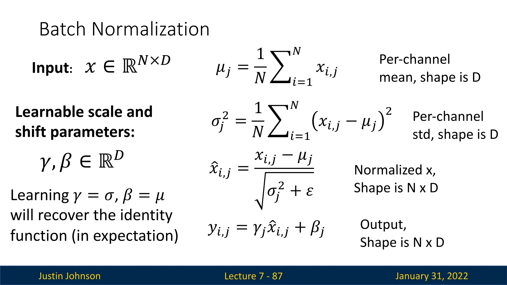
Why is this flexibility useful? During backpropagation, the gradient of the loss with respect to \( x_i \) is given by:
\begin {equation} \frac {dL}{dx_i} = \frac {\gamma _i}{\sqrt {\sigma ^2_B + \epsilon }} \cdot \frac {dL}{dy_i} \end {equation}
Because \( \gamma _i \) is learnable, the network can scale gradients dynamically for each feature, preventing them from becoming too small or too large. The denominator \( \sqrt {\sigma ^2_B + \epsilon } \), derived from the batch statistics, helps stabilize gradient magnitude by normalizing across different activation scales.
This ability to fine-tune the normalized outputs and adaptively control gradient magnitudes helps improve convergence and optimization stability. As we will explore later, the benefits of BatchNorm go far beyond reducing internal covariate shift—they include better conditioning, smoother loss landscapes, and improved robustness during training.
Batch Normalization for Convolutional Neural Networks (CNNs)
Batch Normalization was initially introduced for fully connected (FC) layers, where normalization is performed across the batch dimension. However, in convolutional layers, activations have an additional spatial structure due to the height (\(H\)) and width (\(W\)) dimensions of the feature maps. To adapt Batch Normalization for CNNs, we extend the normalization over both the batch dimension (\(N\)) and spatial dimensions (\(H, W\)).
Instead of computing the mean and variance per feature across only the batch dimension, in CNNs we compute these statistics across the entire feature map. For an input tensor \(X\) of shape \( (N, C, H, W) \), BatchNorm is applied independently to each of the \(C\) feature maps, normalizing over all pixels in \(H \times W\) and all samples in the batch:
\begin {equation} \mu _c = \frac {1}{N H W} \sum _{n=1}^{N} \sum _{h=1}^{H} \sum _{w=1}^{W} x_{nchw} \end {equation}
\begin {equation} \sigma _c^2 = \frac {1}{N H W} \sum _{n=1}^{N} \sum _{h=1}^{H} \sum _{w=1}^{W} (x_{nchw} - \mu _c)^2 \end {equation}
The computed mean and variance are then used to normalize each feature map:
\begin {equation} \hat {x}_{nchw} = \frac {x_{nchw} - \mu _c}{\sqrt {\sigma _c^2 + \epsilon }} \end {equation}
Similar to fully connected layers, learnable parameters \( \gamma _c \) and \( \beta _c \) allow the network to restore any necessary transformations:
\begin {equation} y_{nchw} = \gamma _c \hat {x}_{nchw} + \beta _c \end {equation}
where \( \gamma _c \) and \( \beta _c \) are channel-wise scaling and shifting parameters, ensuring that each feature map can maintain flexibility in representation learning.
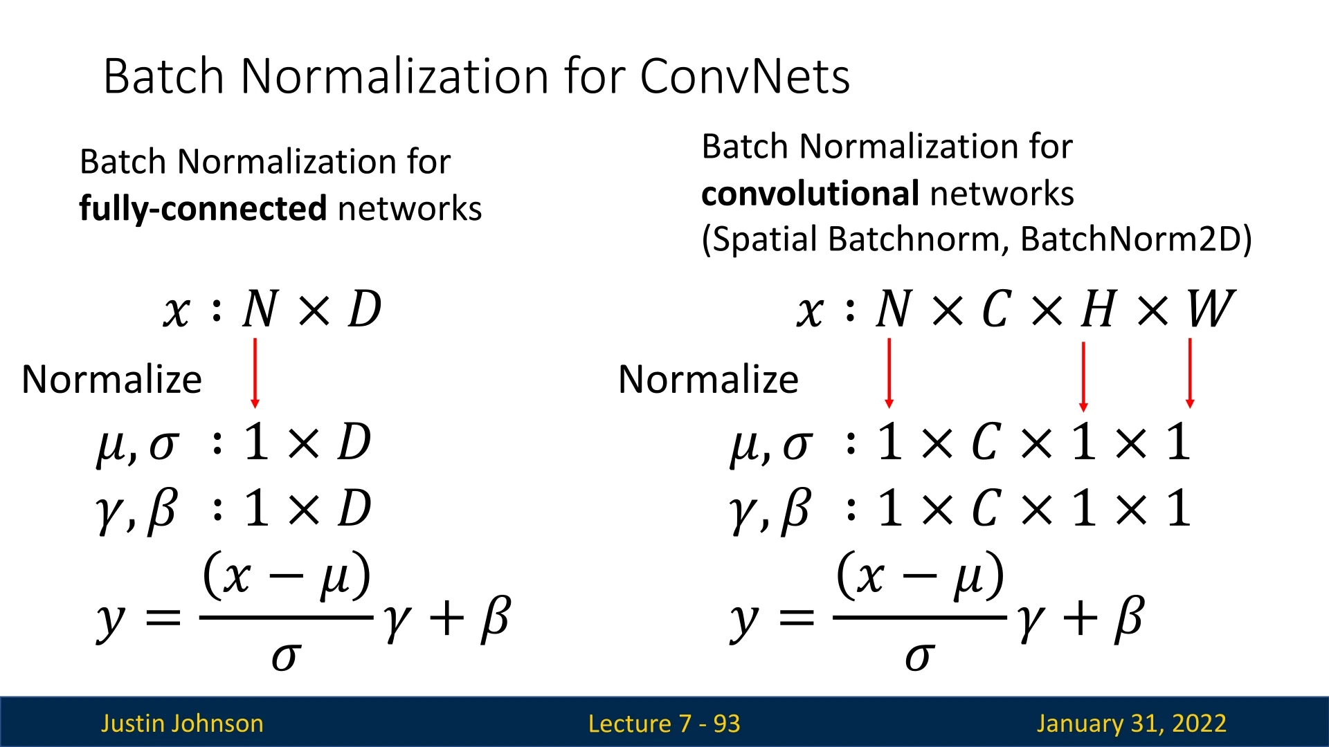
7.11.4 Batch Normalization and Optimization
Beyond Covariate Shift: Why Does BatchNorm Improve Training?
Santurkar et al. (2018) [564] challenged the notion that eliminating internal covariate shift is the key benefit of BatchNorm. They conducted experiments comparing networks trained with BatchNorm under three different conditions:
- Standard: A VGG network trained without BatchNorm.
- Standard + BatchNorm: The same network trained with BatchNorm.
- Standard + ”Noisy” BatchNorm: A BatchNorm-enhanced network where artificial noise was added to induce internal covariate shift (ICS).
Surprisingly, the third setting (which artificially increased internal covariate shift) performed similarly to standard BatchNorm and significantly better than the network without BatchNorm. This suggests that reducing covariate shift is not the primary reason for BatchNorm’s success.
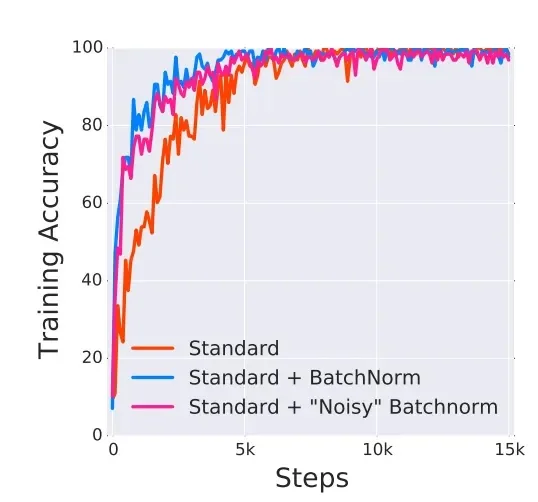
Hence, the authors suggest that secret behind the impact of Batch Normalization is different. Further experiments they conducted suggest that its power comes mainly from smoothing the loss landscape, making training more stable and efficient. The research paper introducing BatchNorm demonstrated that applying it to deep networks leads to a significant reduction in sharp spikes in the loss function.
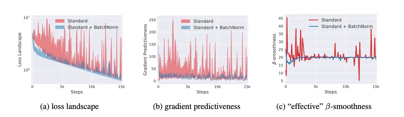
A smoother loss landscape provides several advantages:
- Higher Learning Rates: With reduced variance in activations, the network can tolerate higher learning rates without divergence.
- Reduced Regularization Needs: Since BatchNorm prevents sharp fluctuations, models can often train without excessive weight decay or dropout.
- Faster Convergence: Optimizers can traverse the loss landscape more efficiently, reducing training time.
Why Does BatchNorm Smooth the Loss Surface?
Batch Normalization has been shown empirically to improve optimization dynamics by smoothing the loss surface and allowing for more stable, faster convergence. While several hypotheses attempt to explain these benefits, the precise mechanism is still an active area of research. Below we outline the leading explanations, supported by both experimental evidence and partial theoretical justification.
1. Hessian Eigenvalues and Loss Surface Curvature To understand how BatchNorm influences the loss surface, we first recall the concept of eigenvalues and eigenvectors. Given a square matrix \( A \), an eigenvector \( v \) and its corresponding eigenvalue \( \lambda \) satisfy:
\begin {equation} A v = \lambda v \end {equation}
This means that \( A \) scales \( v \) by \( \lambda \) without changing its direction. The eigenvalues \( \lambda \) indicate the magnitude of stretching or compression in different directions.
Computing Eigenvalues Eigenvalues are computed by solving the characteristic equation:
\begin {equation} \det (A - \lambda I) = 0 \end {equation}
where \( I \) is the identity matrix and \( \det \) denotes the determinant. The roots of this equation give the eigenvalues of \( A \), providing insight into how transformations affect different directions in the space.
Interpretation of Eigenvalues Eigenvalues provide information on how much the function expands or contracts in specific directions:
- Large eigenvalues \( \lambda \) \( \Rightarrow \) significant stretching along that direction.
- Small eigenvalues \( \lambda \) \( \Rightarrow \) minimal effect in that direction.
- Negative eigenvalues \( \Rightarrow \) reversal in direction (indicative of saddle points or local maxima in optimization).
In the context of optimization, the Hessian matrix \( H \) captures the second-order partial derivatives of the loss function:
\begin {equation} H_{ij} = \frac {\partial ^2 \mathcal {L}}{\partial \theta _i \partial \theta _j} \end {equation}
where \( \theta \) represents trainable parameters of the model. The eigenvalues of \( H \) provide insights into the curvature of the loss surface:
- Large eigenvalues \( \lambda \) \( \Rightarrow \) sharp curvature \( \Rightarrow \) unstable gradients and high sensitivity to small parameter updates.
- Small eigenvalues \( \lambda \) \( \Rightarrow \) flatter curvature \( \Rightarrow \) more stable gradients but potentially slower learning.
Empirical studies show that BatchNorm reduces the largest eigenvalues of \( H \), effectively smoothing the loss surface [564]. Researchers assume it occurs because:
- Controlling Activation Magnitudes: Without BN, activations may fluctuate widely, leading to extreme gradient updates. BN normalizes activations, keeping gradients in check and preventing steep loss curvatures.
- Reducing Sensitivity to Parameter Updates: By standardizing activations, small changes in parameters no longer produce unpredictable shifts in the loss function. This keeps the gradient flow stable, preventing large variations in the loss landscape.
2. Reducing the Lipschitz Constant The Lipschitz constant \(L\) quantifies how sensitive the loss function is to parameter changes:
\begin {equation} \| f(x_1) - f(x_2) \| \leq L \| x_1 - x_2 \| \end {equation}
A high \(L\) means that small parameter changes can cause large fluctuations in the loss, making optimization unstable. Since the Lipschitz constant is upper-bounded by the largest eigenvalue of \(H\), reducing the Hessian eigenvalues effectively lowers \(L\), making gradient-based optimization more stable and allowing for larger learning rates without oscillations or divergence.
3. Implicit Regularization via Mini-Batch Noise During training, each mini-batch is normalized with its own mean and variance, leading to slight fluctuations in the forward pass across iterations. This acts as a mild form of noise, conferring several regularization benefits:
- Encourages Broader Optima: Since the model repeatedly sees small variations in its activation distributions, it must learn features robust to those shifts. This steers optimization toward flatter, more generalizable minima.
- Acts Like Mild Data Augmentation: The random normalization offsets per batch resemble an on-the-fly perturbation of inputs/activations, preventing overfitting to a single “static” distribution of feature maps.
4. Decoupling Weight Norm from Direction: A Geometric Reparameterization Perhaps the most compelling theoretical insight comes from interpreting BatchNorm as a reparameterization of weight space. It effectively decouples the magnitude and direction of the weight vector [313].
Let the output of a unit be:
\[ f(w) = \mathbb {E}_x[\phi (x^\top w)], \]
where \( \phi \) is an activation function, and \( x \sim \mathcal {N}(0, S) \) with covariance matrix \( S \succ 0 \). After BatchNorm (ignoring bias for simplicity), this becomes:
\[ f_{\mbox{BN}}(w, \gamma ) = \mathbb {E}_x\left [\phi \left (\gamma \frac {x^\top w}{\sqrt {w^\top S w}}\right )\right ]. \]
This can be rewritten as:
\[ f_{\mbox{BN}}(w, \gamma ) = \mathbb {E}_x\left [\phi \left (x^\top \tilde {w} \right )\right ], \quad \mbox{where } \tilde {w} = \gamma \cdot \frac {w}{\| w \|_S}. \]
The direction of \( w \) is now normalized (via \( \| w \|_S = \sqrt {w^\top S w} \)), and its magnitude is controlled separately via \( \gamma \). This decoupling stabilizes training because the optimization landscape becomes more symmetric and less sensitive to the absolute scaling of weights. It also allows faster convergence in practice.
5. Stabilizing Deep Networks and Preventing Dead Activations BatchNorm helps stabilize deep networks by maintaining well-scaled and centered activations across layers. This is particularly important in networks using non-linearities like ReLU, which zero out all negative inputs. Without normalization, small shifts in weights or biases can cause many activations to fall below zero, pushing neurons into the so-called dead zone, where their output becomes identically zero and gradients cease to flow.
By normalizing pre-activation values to have zero mean and unit variance, BatchNorm ensures that inputs to ReLU are consistently distributed around the activation threshold. This keeps more neurons active during training and reduces the chance of units becoming permanently inactive due to poor initialization or noisy updates. In doing so, it preserves the expressiveness of the network and improves gradient propagation, particularly in deep architectures.
Conclusion: Why BatchNorm Helps—With Caution
Although BatchNorm was originally introduced to reduce internal covariate shift, subsequent empirical and theoretical work suggests that its most impactful contribution lies elsewhere: in stabilizing training dynamics and smoothing the loss surface. By normalizing activations across mini-batches, it helps keep gradients well-scaled, mitigates the risk of exploding or vanishing updates, and allows for the use of larger learning rates.
However, it’s important to emphasize that the precise mechanism by which BatchNorm smooths the optimization landscape is still an area of active research. While studies have demonstrated effects such as reduced Hessian eigenvalues and improved gradient predictability [565], these results are largely empirical and do not yet constitute a unified theoretical explanation. The improvement in trainability may stem from a combination of factors—including length-direction decoupling, Lipschitz control, and others.
This evolving understanding has motivated the development of alternative normalization methods such as Layer Normalization (LN), Instance Normalization (IN), and Group Normalization (GN), which attempt to preserve the optimization benefits of BatchNorm while avoiding its reliance on batch-level statistics. These techniques are particularly useful in settings such as recurrent networks, small-batch training, or generative models, where BatchNorm may be less effective. We will explore these variants in detail in the following sections.
Batch Normalization in Test Time
One challenge with Batch Normalization as presented so far is that the estimated mean and standard deviation depend on the batch statistics, making it impractical for inference where a single input or dynamically arriving data must be processed independently. For example, in a real-time web service where users upload data at unpredictable times, a network that depends on batch statistics would yield inconsistent predictions depending on the users uploading at any moment. This is a critical issue for deploying machine learning models.
To address this, BatchNorm behaves differently during training and testing. During training, the layer operates as described—computing mean and variance over the current batch. However, during inference, instead of relying on batch statistics, the mean and variance are fixed constants obtained from a running average accumulated during training over all batches.
This has two key benefits:
- It restores independence among test-time samples, ensuring consistency.
- It makes the layer effectively linear during inference, meaning it can be merged with the preceding convolution or fully connected layer, introducing no extra computational cost at inference.
Since BatchNorm is typically applied directly after FC/Conv layers but before activation functions (e.g., ReLU), this property is particularly useful, as these can be grouped together, removing the computational overhead of applying BN.
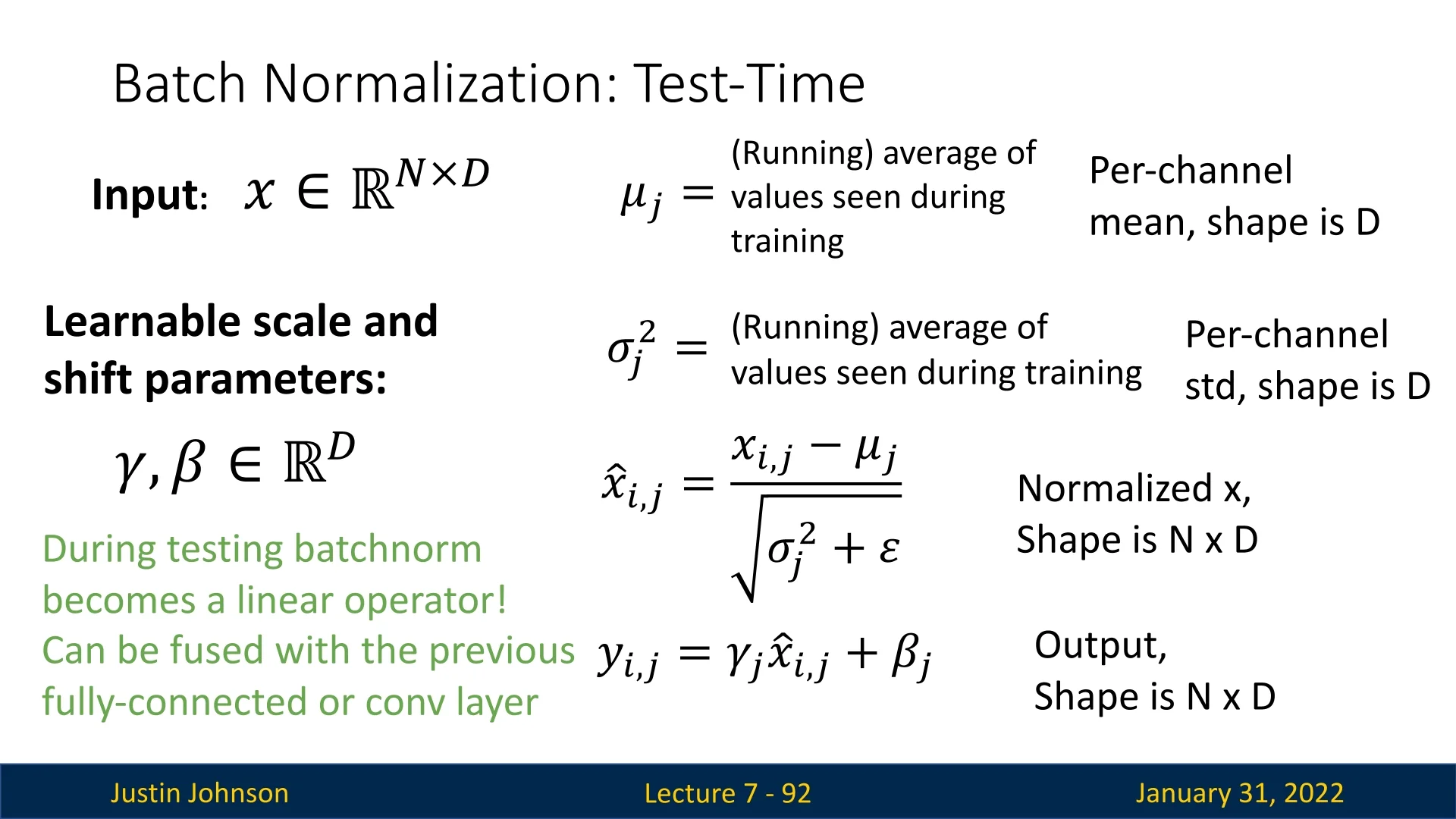
Limitations of BatchNorm
Despite its effectiveness, BatchNorm has several downsides:
- Fixed mean and variance can fail with imbalanced data: If the dataset contains highly imbalanced distributions, the running mean and variance might not generalize well, leading to poor normalization at test time.
- Ineffective for small batch sizes or online learning: Since BatchNorm relies on batch statistics, it does not perform well when batch sizes are small or variable, such as in online learning settings.
- Not suitable for sequential models: Since BatchNorm computes statistics across the batch dimension, it does not naturally fit recurrent architectures like RNNs, which process data sequentially. In addition, it is not suitable for batches of varying sizes (which is often the case with many-to-many or many-to-one problems, which are the ones RNNs and Transformers can solve but regular CNNs/FC networks aren’t built to). Not only that, it is hard to parallellize batch-normalized models, which is critical for Transformers.
- Train-Test Mode Switching Can Cause Bugs: BN requires explicit mode switching between training & inference. Failing to do so can lead to performance degradation if, for instance, the model mistakenly computes statistics from a single test sample as if it were a full batch.
Enrichment 7.14.5: Batch Normalization Placement
Question: In a neural network layer of the form \(\mathbf {z} = \phi (\mathbf {W}\mathbf {x} + \mathbf {b})\), should we apply Batch Normalization (BN) before or after the activation \(\phi \)?
Batch Normalization Placement: Typical Ordering
As introduced in [265], Batch Normalization is most often placed before the nonlinearity (activation) in each layer, i.e.: \[ \mathbf {x} \xrightarrow {\quad \mathrm {linear}\quad } \mathbf {u} \;=\; \mathbf {W}\mathbf {x} + \mathbf {b} \;\xrightarrow {\quad \mathrm {BN}\quad } \widehat {\mathbf {u}} \;\xrightarrow {\quad \phi (\cdot )\quad } \mathbf {z}. \] Specifically:
- Why after the linear part? BN aims to ensure the inputs to the nonlinearity, \(\mathbf {u}\), have more stable means and variances across different mini-batches and training epochs. By centering and scaling \(\mathbf {u}\), BN helps prevent saturating nonlinearities (e.g., sigmoids or \(\tanh \)) from entering their flat regimes, and also stabilizes the gradient flow [265].
- If BN were after the activation: Then the activation \(\phi (\mathbf {u})\) might saturate or shift significantly, and BN would see (and normalize) a distribution that is already “warped”. This often diminishes BN’s ability to regulate the input distribution to the next layer. Empirically, BN-before-activation is widely used (e.g., in [215, 265]).
Mathematical Rationale Denoting \(\mathbf {u} = \mathbf {W}\mathbf {x} + \mathbf {b}\), BN normalizes each scalar coordinate \(u^{(k)}\) to \[ \hat {u}^{(k)} \;=\; \frac {u^{(k)} - \mu _{B}^{(k)}}{\sqrt {\sigma _{B}^{(k)\,2}+\varepsilon }} \;\;\mbox{and then learns two parameters}\;\;\gamma ^{(k)},\;\beta ^{(k)} \;\mbox{to produce}\;\; \gamma ^{(k)} \,\hat {u}^{(k)} + \beta ^{(k)}. \] Placing BN before \(\phi \) effectively keeps the distribution of pre-activation \(\mathbf {u}\) stable as training progresses, letting the subsequent nonlinearity see consistently normalized data.
7.11.5 Alternative Normalization Methods (LN, IN, GN, ...)
Despite BatchNorm’s widespread success, it has drawbacks—particularly with small or non-i.i.d. batches. Various alternatives have emerged to address these limitations:
- Layer Normalization (LN): Normalizes activations across all features for each individual sample, making it batch-size independent; commonly used in RNNs and Transformers.
- Instance Normalization (IN): Applied channel-wise per example (per instance), often in style-transfer tasks where batch statistics are less meaningful.
- Group Normalization (GN): Partitions channels into smaller groups before normalizing; designed for cases (e.g., small batch training) where BatchNorm struggles.
In many CNN applications with large batches, BatchNorm still tends to excel. However, when batch sizes are tiny or data isn’t i.i.d. per batch—such as in Transformers or reinforcement learning—layer normalization or group normalization can prove more stable.
Layer Normalization (LN)
Core Idea Layer Normalization (LN) operates per training example, normalizing across all features of a single sample rather than across a batch. Unlike Batch Normalization (BN), which depends on batch-level statistics, LN is fully independent of batch size. This makes it particularly well-suited for small-batch or single-sequence settings, such as RNNs and Transformers.
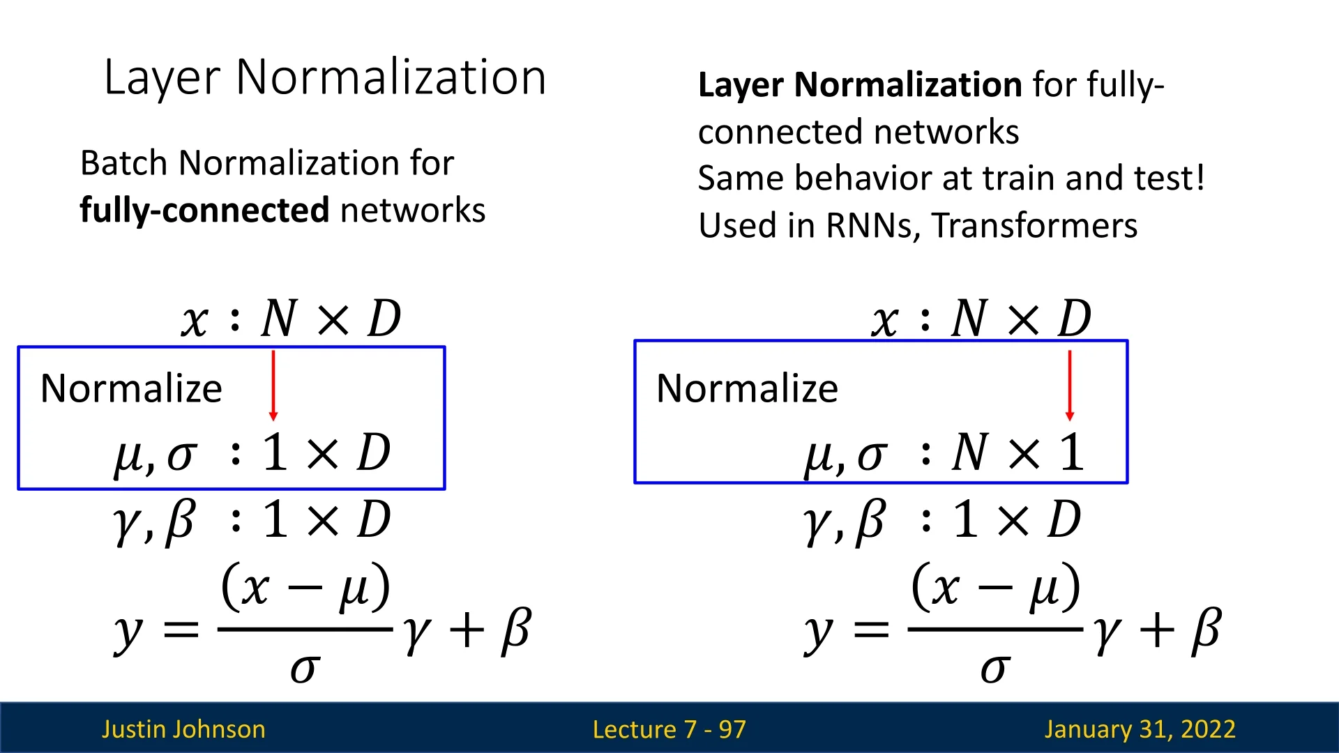
Definition (Fully Connected Layers) Given an input vector \(\mathbf {x} \in \mathbb {R}^N\) corresponding to a single training example: \[ \mu (\mathbf {x}) = \frac {1}{N} \sum _{i=1}^N x_i, \qquad \sigma ^2(\mathbf {x}) = \frac {1}{N} \sum _{i=1}^N \left (x_i - \mu (\mathbf {x})\right )^2. \] Each feature is then normalized as: \[ y_i = \gamma _i \, \frac {x_i - \mu (\mathbf {x})}{\sqrt {\sigma ^2(\mathbf {x}) + \epsilon }} + \beta _i, \quad \mbox{for } i = 1, \dots , N, \] where \(\gamma _i\) and \(\beta _i\) are learnable parameters (per feature), and \(\epsilon \) is a small constant for numerical stability.
Extension to Convolutional Layers For CNNs, LN is applied across all channels and spatial dimensions of each sample independently. For an input tensor \(x \in \mathbb {R}^{N \times C \times H \times W}\), LN is computed per sample \(n\) as: \[ \mu _n = \frac {1}{CHW} \sum _{i=1}^{C} \sum _{j=1}^{H} \sum _{k=1}^{W} x_{nijk}, \qquad \sigma _n^2 = \frac {1}{CHW} \sum _{i=1}^{C} \sum _{j=1}^{H} \sum _{k=1}^{W} \left (x_{nijk} - \mu _n\right )^2. \] Then, each activation \(x_{nijk}\) is normalized as: \[ \hat {x}_{nijk} = \frac {x_{nijk} - \mu _n}{\sqrt {\sigma _n^2 + \epsilon }}, \] followed by learnable scale and shift parameters \(\gamma \), \(\beta \).
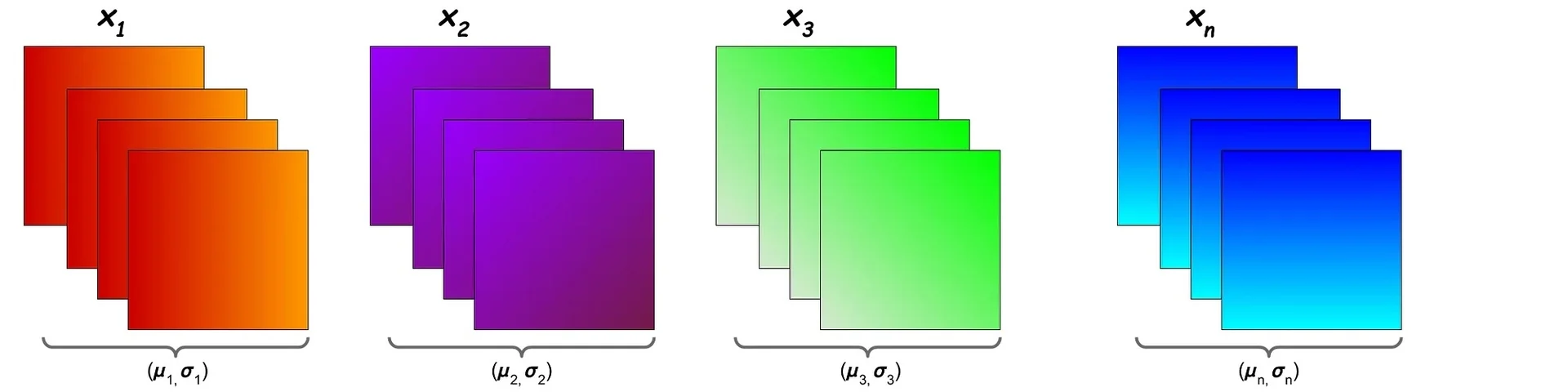
- Per-Sample Aggregation: LN aggregates statistics across features within each sample (vector or image), resulting in consistent normalization that doesn’t depend on other samples in the batch.
- Spatial and Channel Awareness: For images, LN computes a single mean and variance for all pixels and channels in one image, enabling normalization across spatial and semantic dimensions.
- Batch-Size Independence: Since LN doesn’t use inter-sample statistics, it performs well even with very small batches, including batch size 1.
Advantages of Layer Normalization
- 1.
- Robustness to Small Batches: LN remains stable and effective in scenarios where batch sizes are small or variable—such as in reinforcement learning, online learning, or NLP inference.
- 2.
- Essential for Sequence Models: LN is widely adopted in architectures like Transformers and RNNs, where input is typically processed one example (or one time step) at a time. Transformer blocks apply LN after self-attention and feedforward layers to stabilize training and improve convergence.
Instance Normalization (IN)
A more common normalization approach for images, that resembles layer normalization but makes more sense for a CNN use-case (as it applies per feature map, averaging only over the spatial dimensions, and not on the entirety of the input tensor, across all of the channels).
Definition: For each sample \(n\) and channel \(c\), instance normalization computes the mean and variance across the spatial dimensions \((H \times W)\) only:
\begin {equation} \mu _{n c} = \frac {1}{H W} \sum _{j=1}^{H} \sum _{k=1}^{W} x_{n c j k}, \quad \sigma _{n c}^2 = \frac {1}{H W} \sum _{j=1}^{H} \sum _{k=1}^{W} \bigl (x_{n c j k}-\mu _{n c}\bigr )^2. \end {equation}
Then, each activation \(x_{n c j k}\) is normalized as:
\begin {equation} \hat {x}_{n c j k} = \frac {x_{n c j k}-\mu _{n c}}{\sqrt {\sigma _{n c}^2+\epsilon }}, \end {equation}
often followed by learnable scale and shift parameters \((\gamma _c,\,\beta _c)\).
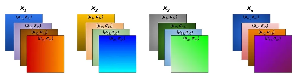
Interpretation Instance Normalization operates at a more granular level than BatchNorm, normalizing each channel within a single image rather than across a batch. This ensures that:
- Each Sample is Treated Independently: Since normalization is applied per sample, IN prevents dependency on batch statistics, which is useful in domains where batch sizes vary significantly.
- Local Contrast is Preserved: Unlike BatchNorm, which normalizes across the batch, IN ensures that fine details remain within individual images while still removing global contrast variations.
Advantages of Instance Normalization
- Batch-Size Independence: Unlike BatchNorm, IN does not rely on batch statistics, making it suitable for applications with small or varying batch sizes.
- Better Style Transfer: By normalizing each sample independently, IN effectively removes contrast variations, enabling consistent style adaptation in tasks such as AdaIN (Adaptive Instance Normalization).
- Effective for Image Generation Tasks: IN helps maintain style consistency in generative models, particularly in GANs and neural style transfer networks.
Group Normalization (GN)
Definition: Group Normalization (GN) normalizes activations across a defined number of groups instead of across the batch (BatchNorm) or spatial dimensions (InstanceNorm). Given a sample \(n\) and a set of \(G\) groups, GN computes the mean and variance for each group across the channels \(C\) and spatial dimensions \(H \times W\):
\begin {equation} \mu _{n g} = \frac {1}{|G| H W} \sum _{c \in G} \sum _{j=1}^{H} \sum _{k=1}^{W} x_{n c j k}, \quad \sigma _{n g}^2 = \frac {1}{|G| H W} \sum _{c \in G} \sum _{j=1}^{H} \sum _{k=1}^{W} \bigl (x_{n c j k}-\mu _{n g}\bigr )^2. \end {equation}
Each activation \(x_{n c j k}\) is then normalized as:
\begin {equation} \hat {x}_{n c j k} = \frac {x_{n c j k}-\mu _{n g}}{\sqrt {\sigma _{n g}^2+\epsilon }}, \end {equation}
followed by learnable scale and shift parameters \((\gamma _c, \beta _c)\).
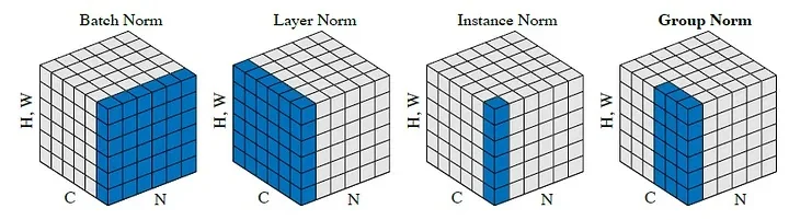
Interpretation Group Normalization introduces an intermediate normalization strategy:
- More Structured than IN: Unlike IN, which normalizes per channel, GN groups multiple channels together, maintaining more structural consistency across activations.
- Avoids Batch Dependency: Unlike BN, GN does not require large batch sizes, making it useful for applications with memory constraints or small datasets.
Advantages of Group Normalization
- Robust to Batch Size: GN does not depend on batch statistics, making it ideal for small-batch training or scenarios where batch sizes vary dynamically.
- Balanced Between BN and IN: GN is more flexible than IN while avoiding the batch dependency of BN.
- Better Regularization: GN effectively captures feature dependencies by normalizing groups of channels together, reducing sensitivity to changes in activation distributions.
- Applicable in Various Architectures: GN is particularly effective in object detection and segmentation tasks where batch sizes tend to be small due to high-resolution inputs.
Why Do IN, LN, and GN Improve Optimization?
While Batch Normalization (BN) has been shown empirically to accelerate and stabilize training—often attributed to “smoothing the loss landscape”—its behavior depends critically on mini-batch statistics, creating instability with small or non-stationary batches. In contrast, Instance Normalization (IN), Layer Normalization (LN), and Group Normalization (GN) normalize feature statistics within each sample or within small groups of features. This per-sample normalization reparameterizes the network such that activations maintain consistent scale and variance, improving gradient behavior and optimization predictability.
Common Benefits Across IN, LN, and GN
- Stabilized Gradient Magnitudes: By normalizing activations to zero mean and unit variance within each sample, these methods constrain the dynamic range of forward activations and backward gradients. This reduces the risk of exploding or vanishing signals, maintaining stable gradient flow throughout training.
- More Predictable Parameter Updates: Because feature distributions remain standardized, weight rescaling or initialization choices have a smaller effect on the magnitude of parameter updates. This produces more uniform effective learning rates across layers and training steps.
- Independence from Batch Size: Unlike BN, which estimates statistics over the mini-batch, IN, LN, and GN compute normalization terms per sample (or per group), making them robust to small, variable, or even unit batch sizes. This ensures identical behavior during training and inference.
Summary: How These Methods Enhance Training Rather than relying on cross-sample averaging to stabilize optimization, IN, LN, and GN regulate feature magnitudes at the sample level, enforcing consistent numerical scales throughout the network:
- Instance Normalization (IN): Normalizes per-sample and per-channel over spatial dimensions (\(H \times W\)), eliminating contrast and illumination variations across instances—especially beneficial in style transfer and low-level vision tasks.
- Layer Normalization (LN): Normalizes across all features within each example. In CNNs, this corresponds to all channels at a single spatial location; in Transformers and RNNs, to all hidden units per token or time step. LN provides stable optimization where batch statistics are unreliable or sequences vary in length.
- Group Normalization (GN): Divides channels into \(G\) groups and normalizes within each group for each sample, balancing IN’s channel locality and LN’s full normalization. GN is particularly effective for CNNs with small or irregular batch sizes.
Together, these normalization schemes stabilize feature distributions, maintain consistent gradient magnitudes, and decouple optimization performance from batch-dependent effects—yielding smoother, more reliable convergence across diverse architectures.
Enrichment 7.14.7: Backpropagation for Batch Normalization
Context and Goal: In a computational-graph framework, \(\mbox{BN}\) (Batch Norm) is viewed as a node receiving input activations \(\mathbf {x}\) and producing outputs \(\mathbf {y}\). Our objective is to compute partial derivatives of an upstream function \(f\) (the next layer’s output) w.r.t. \(\gamma , \beta ,\) and each \(x_i\). Below is the standard BN forward pass:
\[ \begin {aligned} \mu &= \frac {1}{m}\sum _{i=1}^{m} x_i, && \sigma ^2 = \frac {1}{m}\sum _{i=1}^{m} (x_i - \mu )^2, \\ \hat {x}_i &= \frac {x_i - \mu }{\sqrt {\sigma ^2 + \epsilon }}, && y_i = \gamma \,\hat {x}_i + \beta . \end {aligned} \] Here:
- \(\mu ,\sigma ^2\) are the mini-batch mean and variance,
- \(\hat {x}_i\) is the normalized input,
- \(y_i\) is the scaled/shifted output (linear transform),
- \(\gamma ,\beta \) are trainable parameters,
- \(f\) is an upstream layer’s output (e.g., a loss or the next layer’s activation) that depends on \(y\).
Chain Rule in the Graph We consider the node \(\mbox{BN}\) with inputs \(\bigl (\mathbf {x}, \gamma , \beta \bigr )\). The partial derivatives we want are: \[ \frac {\partial f}{\partial x_i}, \quad \frac {\partial f}{\partial \gamma }, \quad \frac {\partial f}{\partial \beta }. \] In a graph sense, “\(\mbox{BN}\) node” receives \(\mathbf {x}\), \(\gamma ,\beta \), and outputs \(\mathbf {y}\) on which the next function \(f\) depends.
Gradients w.r.t. \(\gamma \) and \(\beta \) Recall the output of BatchNorm at each index \(i\) is: \[ y_i = \gamma \,\hat {x}_i + \beta . \] Let \(\frac {\partial f}{\partial y_i}\) be the upstream gradient from the next node in the computational graph (often noted \(\mathrm {dout}[i]\) in code). Applying the chain rule for the local operation \(\hat {x}_i \mapsto y_i\), we get: \[ \frac {\partial f}{\partial \gamma } = \sum _{i=1}^m \underbrace { \frac {\partial f}{\partial y_i} }_{\mbox{upstream}} \times \underbrace { \frac {\partial y_i}{\partial \gamma } }_{\mbox{local} = \hat {x}_i} = \sum _{i=1}^m \Bigl ( \frac {\partial f}{\partial y_i} \;\hat {x}_i \Bigr ), \] \[ \frac {\partial f}{\partial \beta } = \sum _{i=1}^m \underbrace { \frac {\partial f}{\partial y_i} }_{\mbox{upstream}} \times \underbrace { \frac {\partial y_i}{\partial \beta } }_{\mbox{local}=1} = \sum _{i=1}^m \Bigl ( \frac {\partial f}{\partial y_i} \Bigr ). \] Hence, each \(\hat {x}_i\) contributes to \(\frac {\partial f}{\partial \gamma }\), while \(\beta \) accumulates the gradient across all outputs.
Gradient w.r.t. \(\hat {x}_i\) Again by the chain rule, \[ \frac {\partial f}{\partial \hat {x}_i} = \underbrace { \frac {\partial f}{\partial y_i} }_{\mbox{upstream}} \times \underbrace { \frac {\partial y_i}{\partial \hat {x}_i} }_{\mbox{local}=\gamma } = \frac {\partial f}{\partial y_i} \;\gamma . \] Thus, the normalized input \(\hat {x}_i\) receives an upstream gradient scaled by \(\gamma \).
Gradients Involving \(\mu \) and \(\sigma ^2\) The normalized input \(\hat {x}_i\) depends on the batch mean \(\mu \) and variance \(\sigma ^2\): \[ \mu = \frac {1}{m}\sum _{j=1}^m x_j,\quad \sigma ^2 = \frac {1}{m}\sum _{j=1}^m (x_j - \mu )^2, \quad \hat {x}_i = \frac {x_i - \mu }{\sqrt {\sigma ^2+\epsilon }}. \] Hence, to find \(\tfrac {\partial f}{\partial \mu }\) and \(\tfrac {\partial f}{\partial \sigma ^2}\), we first compute local derivatives w.r.t. \(\mu ,\sigma ^2\) and multiply by the upstream gradient \(\tfrac {\partial f}{\partial \hat {x}_i}\). Formally: \[ \frac {\partial f}{\partial \sigma ^2} = \sum _{i=1}^m \Bigl ( \underbrace { \frac {\partial f}{\partial \hat {x}_i} }_{\mbox{upstream}} \times \underbrace { \frac {\partial \hat {x}_i}{\partial \sigma ^2} }_{\mbox{local}} \Bigr ), \quad \frac {\partial f}{\partial \mu } = \sum _{i=1}^m \Bigl [ \underbrace { \frac {\partial f}{\partial \hat {x}_i} \times \frac {\partial \hat {x}_i}{\partial \mu } }_{\mbox{direct}} \;+\; \underbrace { \frac {\partial f}{\partial \sigma ^2} \times \frac {\partial \sigma ^2}{\partial \mu } }_{\mbox{indirect}} \Bigr ]. \] Deriving each partial (e.g. \(\tfrac {\partial \hat {x}_i}{\partial \sigma ^2}\), \(\tfrac {\partial \sigma ^2}{\partial \mu }\), etc.) involves basic calculus on the above definitions.
Final: Gradients w.r.t. Each \(x_i\) Each input \(x_i\) influences \(\hat {x}_i\), \(\mu \), and \(\sigma ^2\). By the chain rule, we combine all relevant paths: \[ \frac {\partial f}{\partial x_i} = \underbrace { \frac {\partial f}{\partial \hat {x}_i} \times \frac {\partial \hat {x}_i}{\partial x_i} }_{\mbox{direct path}} \;+\; \underbrace { \frac {\partial f}{\partial \mu } \times \frac {\partial \mu }{\partial x_i} }_{\mbox{indirect via mean}} \;+\; \underbrace { \frac {\partial f}{\partial \sigma ^2} \times \frac {\partial \sigma ^2}{\partial x_i} }_{\mbox{indirect via variance}}. \]
Careful algebraic manipulation of these terms leads to the well-known ”batchnorm backward” formula, which is often expressed in compact summations (e.g., \(\sum _i \frac {\partial f}{\partial \hat {x}_i} \hat {x}_i\)). If you’re interested in a more detailed step-by-step derivation, including further simplifications and an efficient implementation, Kevin Zakka provides an excellent breakdown in his blog post [772]. His explanation follows a structured approach to deriving the gradients and includes an optimized implementation of the backpropagation process.
Computational Efficiency Though the above derivatives look cumbersome, summation terms (like \(\sum _i \tfrac {\partial f}{\partial \hat {x}_i}\,\hat {x}_i\)) are typically computed once per batch. This staged approach significantly reduces redundant calculations.
Extension to LN, IN, GN The same chain-rule derivation applies to layer, instance, or group normalization, changing only which axes are used for \(\mu \) and \(\sigma ^2\). In all cases, the node perspective remains: \[ \mbox{(in) } \to [\mu , \sigma ^2] \to \hat {x} \to [\gamma ,\beta ] \to \mbox{(out).} \] Hence the backward pass is conceptually the same, ensuring one can unify the code logic with minor changes to which dimensions are averaged.
Conclusion Treating BN as a node in the computational graph clarifies how gradients w.r.t. \(\gamma \), \(\beta \), and \(\{x_i\}\) are computed step by step. Although the algebra is more involved than standard layers, frameworks typically perform these summations under the hood, allowing practitioners to reap BN’s benefits with minimal overhead.
Enrichment 7.14.8: Batch Normalization & \(\ell _2\) Regularization
Context and References This discussion builds upon classic results on \(\ell _2\) regularization (as in §7.14) and batch normalization, and draws heavily from the excellent analysis by Jane Street’s tech blog [612]. Their exposition highlights the subtle—but critical—interactions between BN and weight decay in modern architectures. What follows summarizes and expands on their findings with mathematical and practical clarifications.
1. \(\ell _2\) Regularization Without BatchNorm In traditional training, \(\ell _2\) regularization (also called weight decay) adds a penalty to the loss: \[ \mathrm {Loss}(w, x) = \underbrace {\mathcal {L}(f(w, x), y)}_{\mbox{DataLoss}} + \frac {1}{2}c \|w\|^2, \] where \(\mathcal {L}\) is a standard loss (e.g., cross-entropy), and \(c > 0\) is the weight decay coefficient.
Taking the gradient and applying SGD yields: \[ \frac {\partial \mathrm {Loss}}{\partial w} = \nabla \mathcal {L}(f(w, x), y) + c w \quad \Longrightarrow \quad w \gets w - \alpha \bigl (\nabla \mathcal {L} + c w\bigr ), \] which simplifies to: \[ w \gets (1 - \alpha c)\, w - \alpha \nabla \mathcal {L}. \] So weight decay shrinks weights with each update, and thus, reduces the model’s capacity to ”memorize” noise in the training set. Here’s one way to understand this:
- If a weight \(w_i\) truly helps the model reduce the loss on a wide range of samples, it will get pushed up by gradients consistently and ”fight back” against decay.
- If \(w_i\) mostly captures noise (e.g., a rare correlation or one-off pattern), its gradient updates will be weak and inconsistent. Decay will eventually shrink it away.
This mechanism biases the model toward parameters that reflect broad, reliable structure in the data and away from those that overfit idiosyncrasies.
From a Bayesian lens, \(\tfrac 12 c \|w\|^2\) is equivalent to placing a Gaussian prior \(w \sim \mathcal {N}(0, \tfrac {1}{c} I)\) over the weights. This penalizes ”complex” functions with highly varying outputs (which often require large weights), and favors ”simpler” smoother functions that generalize better.
2. BN Cancels Weight Norm in the Forward Pass Let \(L(w)\) be the pre-BN output of a convolutional or linear layer. BN transforms it as: \[ \mathrm {BN}(L(w)) = \gamma \cdot \frac {L(w) - \mu _L}{\sqrt {\sigma _L^2 + \varepsilon }} + \beta , \] where \(\mu _L\) and \(\sigma _L\) are the batch-wise mean and standard deviation, and \(\gamma , \beta \) are learnable scale and shift parameters.
Now suppose weight decay acts to scale \(w \mapsto \lambda w\), where \(\lambda < 1\). Then: \[ L(\lambda w) = \lambda L(w), \quad \mu _L(\lambda w) = \lambda \mu _L(w), \quad \sigma _L(\lambda w) = \lambda \sigma _L(w), \] so: \[ \mathrm {BN}(L(\lambda w)) = \gamma \cdot \frac {\lambda L(w) - \lambda \mu _L(w)}{\lambda \sigma _L(w)} + \beta = \mathrm {BN}(L(w)). \]
Importantly: This result is unaffected by \(\gamma \) and \(\beta \) — they operate after the scale-invariance has already been enforced. That is, even with \(\gamma , \beta \), BN cancels any uniform rescaling of \(w\). Hence, from a forward-pass perspective, \(\ell _2\)’s pressure to ”shrink” weights becomes meaningless when followed by BN. This is precisely where the confusion arises.
3. Why \(\ell _2\) Still Matters: Learning Dynamics Perspective Although BN erases the influence of weight norm in the forward pass, it does not erase it in the gradient computation. To see this, recall that BN includes a normalization step: \[ \hat {z} = \frac {z - \mu }{\sqrt {\sigma ^2 + \varepsilon }}, \quad \mbox{with } z = L(w). \]
Now, using the chain rule: \[ \frac {\partial \, \mathrm {BN}(L(w))}{\partial w} = \frac {\partial \, \mathrm {BN}}{\partial z} \cdot \frac {\partial z}{\partial w}. \]
Since \(L(w)\) is a linear function of \(w\), and \(\mathrm {BN}\) divides by \(\sigma (L(w))\), which grows proportionally to \(\|w\|\), we find: \[ \frac {\partial \, \mathrm {BN}(L(w))}{\partial w} \sim \frac {1}{\|w\|}. \]
Thus, if \(\|w\|\) becomes large, the gradient shrinks. To see this, assume \(L(w) = x \cdot w\) is a linear operation (dot product or convolution) with a fixed input \(x\). Then: \[ \mbox{Var}(L(w)) = \mbox{Var}(x \cdot w) = \|w\|^2 \cdot \mbox{Var}(x), \] assuming \(x\) has zero mean and uncorrelated components.
Hence, \[ \sigma (L(w)) = \sqrt {\mbox{Var}(L(w))} \propto \|w\|. \]
This means that the batch stddev used in BN grows linearly with the weight norm, and so: \[ \frac {\partial \mathrm {BN}(L(w))}{\partial w} \sim \frac {1}{\|w\|}. \]
As weights grow, the gradient shrinks, reducing the size of updates.
This decreases the effective learning rate, leading to:
- Stalled training: The model’s parameters stop updating significantly.
- Unstable convergence: Weight norms may keep drifting while no learning progress is made.
Weight decay limits this drift, keeping gradients in a healthy range and training stable.
4. Coexisting With Learning Rate Schedules A natural question is whether weight decay might conflict with LR schedules like cosine decay or step-wise reduction (we’ll cover them and others later). In fact, they are complementary:
- Schedulers (e.g., cosine or step decay) reduce the base learning rate \(\alpha \) explicitly.
- Weight decay prevents the unintended implicit decay of step size caused by increasing \(\|w\|\).
- Complementary Gradient Control: By combining weight decay (which stabilizes weight magnitudes) with an explicit learning-rate schedule (which controls gradient scale over time), we maintain smoother training dynamics. This synergy helps the optimizer explore wider valleys in the loss landscape. Empirically, such flatter minima—where the loss changes slowly around the solution—are correlated with better generalization [301, 341]. Weight decay acts as a regularizer that discourages sharp, narrow minima that can overfit to training noise.
5. Behavior of BN’s \(\gamma , \beta \) BN layers include learnable scale and shift: \[ \mathrm {BN}(z) = \gamma \cdot \hat {z} + \beta , \quad \mbox{where} \quad \hat {z} = \frac {z - \mu }{\sqrt {\sigma ^2 + \varepsilon }}. \]
Since BN cancels the effect of weight scale, \(\gamma \) could in principle absorb all scale lost from L2 regularization. However:
- We exclude \(\gamma ,\beta \) from decay. This preserves BN’s ability to scale features.
-
In practice, \(\gamma \) rarely “blows up” to cancel all decay. It adjusts smoothly under SGD. While it’s true that BN has a learnable scale parameter \(\gamma \), it cannot completely negate the effect of weight decay. Here’s why:
- \(\gamma \) is applied after normalization. It cannot recover the rich directional information lost by decaying all filter weights toward zero.
- \(\gamma \) is learned via SGD just like other parameters, and it’s updated based on how useful it is for prediction—not as a compensatory mechanism. There is no strong gradient pressure to “undo” weight decay unless the model explicitly benefits from high post-BN amplitudes.
- Empirically, \(\gamma \) tends to stabilize around moderate values. It may grow slightly in response to decay, but does not explode unless other hyperparameters are poorly tuned (e.g., too large a decay on weights, or poor initialization).
- Thus, \(\ell _2\) still controls learning dynamics by limiting \(\|w\|\) on the main weights.
- Exclude BN’s \(\gamma ,\beta \) from decay. This preserves the intended normalization behavior.
- Tune decay strength. Since L2 is now an optimization stabilizer (not a pure regularizer), lower values often suffice.
- Avoid small batch instability. BN becomes noisy at batch sizes \(< 8\); L2 may exacerbate instability. Consider GroupNorm or adjusting BN momentum.
7. Conclusion: BN & L2 Are Complementary, Not Contradictory Even though BN neutralizes the forward-pass effect of \(\|w\|\), weight decay:
- Prevents gradients from vanishing due to large \(\|w\|\).
- Maintains effective learning rate throughout training.
- Improves convergence and often generalization.
Thus, BN and \(\ell _2\) are not at odds. They act on different parts of the training pipeline: BN stabilizes the forward activations; weight decay stabilizes the optimization trajectory. Used together, they form a synergistic pair in modern architectures.